

Page 1

Page 2

DISTANT SPEECH
RECOGNITION
Distant Speech Recognition Matthias W¨olfel and John McDonough
© 2009 John Wiley & Sons, Ltd. ISBN: 978-0-470-51704-8
Page 3

DISTANT SPEECH
RECOGNITION
Matthias W¨olfel
Universit¨at Karlsruhe (TH), Germany
and
John McDonough
Universit¨at des Saarlandes, Germany
A John Wiley and Sons, Ltd., Publication
Page 4

This edition first published 2009
© 2009 John Wiley & Sons Ltd
Registered office
John Wiley & Sons Ltd, The Atrium, Southern Gate, Chichester, West Sussex, PO19 8SQ, United Kingdom
For details of our global editorial offices, for customer services and for information about how to apply for
permission to reuse the copyright material in this book please see our website at www.wiley.com.
The right of the author to be identified as the author of this work has been asserted in accordance with the
Copyright, Designs and Patents Act 1988.
All rights reserved. No part of this publication may be reproduced, stored in a retrieval system, or transmitted, in
any form or by any means, electronic, mechanical, photocopying, recording or otherwise, except as permitted by
the UK Copyright, Designs and Patents Act 1988, without the prior permission of the publisher.
Wiley also publishes its books in a variety of electronic formats. Some content that appears in print may not be
available in electronic books.
Designations used by companies to distinguish their products are often claimed as trademarks. All brand names
and product names used in this book are trade names, service marks, trademarks or registered trademarks of their
respective owners. The publisher is not associated with any product or vendor mentioned in this book. This
publication is designed to provide accurate and authoritative information in regard to the subject matter covered.
It is sold on the understanding that the publisher is not engaged in rendering professional services. If professional
advice or other expert assistance is required, the services of a competent professional should be sought.
Wiley also publishes its books in a variety of electronic formats. Some content that appears
in print may not be available in electronic books.
Library of Congress Cataloging-in-Publication Data
W¨olfel, Matthias.
Distant speech recognition / Matthias W¨olfel, John McDonough.
p. cm.
Includes bibliographical references and index.
ISBN 978-0-470-51704-8 (cloth)
1. Automatic speech recognition. I. McDonough, John (John W.) II. Title.
TK7882.S65W64 2009
006.4
54–dc22
2008052791
A catalogue record for this book is available from the British Library
ISBN 978-0-470-51704-8 (H/B)
Typeset in 10/12 Times by Laserwords Private Limited, Chennai, India
Printed and bound in Great Britain by Antony Rowe Ltd, Chippenham, Wiltshire
Page 5

Contents
Foreword xiii
Preface xvii
1 Introduction 1
1.1 Research and Applications in Academia and Industry 1
1.1.1 Intelligent Home and Office Environments 2
1.1.2 Humanoid Robots 3
1.1.3 Automobiles 4
1.1.4 Speech-to-Speech Translation 6
1.2 Challenges in Distant Speech Recognition 7
1.3 System Evaluation 9
1.4 Fields of Speech Recognition 10
1.5 Robust Perception 12
1.5.1 A Priori Knowledge 12
1.5.2 Phonemic Restoration and Reliability 12
1.5.3 Binaural Masking Level Difference 14
1.5.4 Multi-Microphone Processing 14
1.5.5 Multiple Sources by Different Modalities 15
1.6 Organizations, Conferences and Journals 16
1.7 Useful Tools, Data Resources and Evaluation Campaigns 18
1.8 Organization of this Book 18
1.9 Principal Symbols used Throughout the Book 23
1.10 Units used Throughout the Book 25
2Acoustics 27
2.1 Physical Aspect of Sound 27
2.1.1 Propagation of Sound in Air 28
2.1.2 The Speed of Sound 29
2.1.3 Wave Equation and Velocity Potential 29
2.1.4 Sound Intensity and Acoustic Power 31
2.1.5 Reflections of Plane Waves 32
2.1.6 Reflections of Spherical Waves 33
Page 6

vi Contents
2.2 Speech Signals 34
2.2.1 Production of Speech Signals 34
2.2.2 Units of Speech Signals 36
2.2.3 Categories of Speech Signals 39
2.2.4 Statistics of Speech Signals 39
2.3 Human Perception of Sound 41
2.3.1 Phase Insensitivity 42
2.3.2 Frequency Range and Spectral Resolution 42
2.3.3 Hearing Level and Speech Intensity 42
2.3.4 Masking 44
2.3.5 Binaural Hearing 45
2.3.6 Weighting Curves 45
2.3.7 Virtual Pitch 46
2.4 The Acoustic Environment 47
2.4.1 Ambient Noise 47
2.4.2 Echo and Reverberation 48
2.4.3 Signal-to-Noise and Signal-to-Reverberation Ratio 51
2.4.4 An Illustrative Comparison between Close and Distant
Recordings 52
2.4.5 The Influence of the Acoustic Environment on Speech Production 53
2.4.6 Coloration 54
2.4.7 Head Orientation and Sound Radiation 55
2.4.8 Expected Distances between the Speaker and the Microphone 57
2.5 Recording Techniques and Sensor Configuration 58
2.5.1 Mechanical C lassification of Microphones 58
2.5.2 Electrical Classification of Microphones 59
2.5.3 Characteristics of Microphones 60
2.5.4 Microphone Placement 60
2.5.5 Microphone Amplification 62
2.6 Summary and Further Reading 62
2.7 Principal Symbols 63
3 Signal Processing and Filtering Techniques 65
3.1 Linear Time-Invariant Systems 65
3.1.1 Time Domain Analysis 66
3.1.2 Frequency Domain Analysis 69
3.1.3 z-Transform Analysis 72
3.1.4 Sampling Continuous-Time Signals 79
3.2 The Discrete Fourier Transform 82
3.2.1 Realizing LTI Systems with the DFT 85
3.2.2 Overlap-Add Method 86
3.2.3 Overlap-Save M ethod 87
3.3 Short-Time Fourier Transform 87
3.4 Summary and Further Reading 90
3.5 Principal Symbols 91
Page 7

Contents vii
4 Bayesian Filters 93
4.1 Sequential Bayesian Estimation 95
4.2 Wiener Filter 98
4.2.1 Time Domain Solution 98
4.2.2 Frequency Domain Solution 99
4.3 Kalman Filter and Variations 101
4.3.1 Kalman Filter 101
4.3.2 Extended Kalman Filter 106
4.3.3 Iterated Extended Kalman Filter 107
4.3.4 Numerical Stability 108
4.3.5 Probabilistic Data Association Filter 110
4.3.6 Joint Probabilistic Data Association Filter 115
4.4 Particle Filters 121
4.4.1 Approximation of Probabilistic Expectations 121
4.4.2 Sequential Monte Carlo Methods 125
4.5 Summary and Further Reading 132
4.6 Principal Symbols 133
5 Speech Feature Extraction 135
5.1 Short-Time Spectral Analysis 136
5.1.1 Speech Windowing and Segmentation 136
5.1.2 The Spectrogram 137
5.2 Perceptually Motivated Representation 138
5.2.1 Spectral Shaping 138
5.2.2 Bark and Mel Filter Banks 139
5.2.3 Warping by Bilinear Transform – Time vs Frequency Domain 142
5.3 Spectral Estimation and Analysis 145
5.3.1 Power Spectrum 145
5.3.2 Spectral Envelopes 146
5.3.3 LP Envelope 147
5.3.4 MVDR Envelope 150
5.3.5 Perceptual LP Envelope 153
5.3.6 Warped LP Envelope 153
5.3.7 Warped MVDR Envelope 156
5.3.8 Warped-Twice MVDR Envelope 157
5.3.9 Comparison of Spectral Estimates 159
5.3.10 Scaling of Envelopes 160
5.4 Cepstral Processing 163
5.4.1 Definition and Characteristics of Cepstral Sequences 163
5.4.2 Homomorphic Deconvolution 166
5.4.3 Calculating Cepstral Coefficients 167
5.5 Comparison between Mel Frequency, Perceptual LP and warped
MVDR Cepstral Coefficient Front-Ends 168
5.6 Feature Augmentation 169
5.6.1 Static and Dynamic Parameter Augmentation 169
Page 8

viii Contents
5.6.2 Feature Augmentation by Temporal Patterns 171
5.7 Feature Reduction 171
5.7.1 Class Separability Measures 172
5.7.2 Linear Discriminant Analysis 173
5.7.3 Heteroscedastic Linear Discriminant Analysis 176
5.8 Feature-Space Minimum Phone Error 178
5.9 Summary and Further Reading 178
5.10 Principal Symbols 179
6 Speech Feature Enhancement 181
6.1 Noise and Reverberation in Various Domains 183
6.1.1 Frequency Domain 183
6.1.2 Power Spectral Domain 185
6.1.3 Logarithmic Spectral Domain 186
6.1.4 Cepstral Domain 187
6.2 Two Principal Approaches 188
6.3 Direct Speech Feature Enhancement 189
6.3.1 Wiener Filter 189
6.3.2 Gaussian and Super-Gaussian MMSE Estimation 191
6.3.3 RASTA Processing 191
6.3.4 Stereo-Based Piecewise Linear Compensation for Environments 192
6.4 Schematics of Indirect Speech Feature Enhancement 193
6.5 Estimating Additive Distortion 194
6.5.1 Voice Activity Detection-Based Noise Estimation 194
6.5.2 Minimum Statistics Noise Estimation 195
6.5.3 Histogram- and Quantile-Based Methods 196
6.5.4 Estimation of the a Posteriori and a Priori Signal-to-Noise Ratio 197
6.6 Estimating Convolutional Distortion 198
6.6.1 Estimating Channel Effects 199
6.6.2 Measuring the Impulse Response 200
6.6.3 Harmful Effects of Room Acoustics 201
6.6.4 Problem in Speech Dereverberation 201
6.6.5 Estimating Late Reflections 202
6.7 Distortion Evolution 204
6.7.1 Random Walk 204
6.7.2 Semi-random Walk by Polyak Averaging and Feedback 205
6.7.3 Predicted Walk by Static Autoregressive Processes 206
6.7.4 Predicted Walk by Dynamic Autoregressive Processes 207
6.7.5 Predicted Walk by Extended Kalman Filters 209
6.7.6 Correlated Prediction Error Covariance Matrix 210
6.8 Distortion Evaluation 211
6.8.1 Likelihood Evaluation 212
6.8.2 Likelihood Evaluation by a Switching Model 213
6.8.3 Incorporating the Phase 214
6.9 Distortion Compensation 215
Page 9

Contents ix
6.9.1 Spectral Subtraction 215
6.9.2 Compensating for Channel Effects 217
6.9.3 Distortion Compensation for Distributions 218
6.10 Joint Estimation of Additive and Convolutional Distortions 222
6.11 Observation Uncertainty 227
6.12 Summary and Further Reading 228
6.13 Principal Symbols 229
7 Search: Finding the Best Word Hypothesis 231
7.1 Fundamentals of Search 233
7.1.1 Hidden Markov Model: Definition 233
7.1.2 Viterbi Algorithm 235
7.1.3 Word Lattice Generation 238
7.1.4 Word Trace Decoding 240
7.2 Weighted Finite-State Transducers 241
7.2.1 Definitions 241
7.2.2 Weighted Composition 244
7.2.3 Weighted Determinization 246
7.2.4 Weight Pushing 249
7.2.5 Weighted Minimization 251
7.2.6 Epsilon Removal 253
7.3 Knowledge Sources 255
7.3.1 Grammar 256
7.3.2 Pronunciation Lexicon 263
7.3.3 Hidden Markov Model 264
7.3.4 Context Dependency Decision Tree 264
7.3.5 Combination of Knowledge Sources 273
7.3.6 Reducing Search Graph Size 274
7.4 Fast On-the-Fly Composition 275
7.5 Word and Lattice Combination 278
7.6 Summary and Further Reading 279
7.7 Principal Symbols 281
8 Hidden Markov Model Parameter Estimation 283
8.1 Maximum Likelihood Parameter Estimation 284
8.1.1 Gaussian Mixture Model Parameter Estimation 286
8.1.2 Forward– Backward Estimation 290
8.1.3 Speaker-Adapted Training 296
8.1.4 Optimal Regression Class Estimation 300
8.1.5 Viterbi and Label Training 301
8.2 Discriminative Parameter Estimation 302
8.2.1 Conventional Maximum Mutual Information Estimation
Formulae 302
8.2.2 Maximum Mutual Information Training on Word Lattices 306
8.2.3 Minimum Word and Phone Error Training 308
Page 10

x Contents
8.2.4 Maximum Mutual Information Speaker-Adapted Training 310
8.3 Summary and Further Reading 313
8.4 Principal Symbols 315
9 Feature and Model Transformation 317
9.1 Feature Transformation Techniques 318
9.1.1 Vocal Tract Length Normalization 318
9.1.2 Constrained Maximum Likelihood Linear Regression 319
9.2 Model Transformation Techniques 320
9.2.1 Maximum Likelihood Linear Regression 321
9.2.2 All-Pass Transform Adaptation 322
9.3 Acoustic Model Combination 332
9.3.1 Combination of Gaussians in the Logarithmic Domain 333
9.4 Summary and Further Reading 334
9.5 Principal Symbols 336
10 Speaker Localization and Tracking 337
10.1 Conventional Techniques 338
10.1.1 Spherical Intersection Estimator 339
10.1.2 Spherical Interpolation Estimator 341
10.1.3 Linear Intersection Estimator 342
10.2 Speaker Tracking with the Kalman Filter 345
10.2.1 Implementation Based on the Cholesky Decomposition 348
10.3 Tracking Multiple Simultaneous Speakers 351
10.4 Audio-Visual Speaker Tracking 352
10.5 Speaker Tracking with the Particle Filter 354
10.5.1 Localization Based on Time Delays of Arrival 356
10.5.2 Localization Based on Steered Beamformer Response Power 356
10.6 Summary and Further Reading 357
10.7 Principal Symbols 358
11 Digital Filter Banks 359
11.1 Uniform Discrete Fourier Transform Filter Banks 360
11.2 Polyphase Implementation 364
11.3 Decimation and Expansion 365
11.4 Noble Identities 368
11.5 Nyquist(M) Filters 369
11.6 Filter Bank Design of De Haan et al. 371
11.6.1 Analysis Prototype Design 372
11.6.2 Synthesis Prototype Design 375
11.7 Filter Bank Design with the Nyquist(M ) Criterion 376
11.7.1 Analysis Prototype Design 376
11.7.2 Synthesis Prototype Design 377
11.7.3 Alternative Design 378
Page 11

Contents xi
11.8 Quality Assessment of Filter Bank Prototypes 379
11.9 Summary and Further Reading 384
11.10 Principal Symbols 384
12 Blind Source Separation 387
12.1 Channel Quality and Selection 388
12.2 Independent Component Analysis 390
12.2.1 Definition of ICA 390
12.2.2 Statistical Independence and its Implications 392
12.2.3 ICA Optimization Criteria 396
12.2.4 Parameter Update Strategies 403
12.3 BSS Algorithms based on Second-Order Statistics 404
12.4 Summary and Further Reading 407
12.5 Principal Symbols 408
13 Beamforming 409
13.1 Beamforming Fundamentals 411
13.1.1 Sound Propagation and Array Geometry 411
13.1.2 Beam Patterns 415
13.1.3 Delay-and-Sum Beamformer 416
13.1.4 Beam Steering 421
13.2 Beamforming Performance Measures 426
13.2.1 Directivity 426
13.2.2 Array Gain 428
13.3 Conventional Beamforming Algorithms 430
13.3.1 Minimum Variance Distortionless Response Beamformer 430
13.3.2 Array Gain of the MVDR Beamformer 433
13.3.3 MVDR Beamformer Performance with Plane Wave
Interference 433
13.3.4 Superdirective Beamformers 437
13.3.5 Minimum Mean Square Error Beamformer 439
13.3.6 Maximum Signal-to-Noise Ratio Beamformer 441
13.3.7 Generalized Sidelobe Canceler 441
13.3.8 Diagonal Loading 445
13.4 Recursive Algorithms 447
13.4.1 Gradient Descent Algorithms 448
13.4.2 Least Mean Square Error Estimation 450
13.4.3 Recursive Least Squares Estimation 455
13.4.4 Square-Root Implementation of the RLS Beamformer 461
13.5 Nonconventional Beamforming Algorithms 465
13.5.1 Maximum Likelihood Beamforming 466
13.5.2 Maximum Negentropy Beamforming 471
13.5.3 Hidden Markov Model Maximum Negentropy Beamforming 477
13.5.4 Minimum Mutual Information Beamforming 480
13.5.5 Geometric Source Separation 487
Page 12

xii Contents
13.6 Array Shape Calibration 488
13.7 Summary and Further Reading 489
13.8 Principal Symbols 491
14 Hands On 493
14.1 Example Room Configurations 494
14.2 Automatic Speech Recognition Engines 496
14.3 Word Error Rate 498
14.4 Single-Channel Feature Enhancement Experiments 499
14.5 Acoustic Speaker-Tracking Experiments 501
14.6 Audio-Video Speaker-Tracking Experiments 503
14.7 Speaker-Tracking Performance vs Word Error Rate 504
14.8 Single-Speaker Beamforming Experiments 505
14.9 Speech Separation Experiments 507
14.10 Filter Bank Experiments 508
14.11 Summary and Further Reading 509
Appendices 511
A List of Abbreviations 513
B Useful Background 517
B.1 Discrete Cosine Transform 517
B.2 Matrix Inversion Lemma 518
B.3 Cholesky Decomposition 519
B.4 Distance Measures 519
B.5 Super-Gaussian Probability Density Functions 521
B.5.1 Generalized Gaussian pdf 521
B.5.2 Super-Gaussian pdfs with the Meier G-function 523
B.6 Entropy 528
B.7 Relative Entropy 529
B.8 Transformation Law of Probabilities 529
B.9 Cascade of Warping Stages 530
B.10 Taylor Series 530
B.11 Correlation and Covariance 531
B.12 Bessel Functions 531
B.13 Proof of the Nyquist–Shannon Sampling Theorem 532
B.14 Proof of Equations (11.31–11.32) 532
B.15 Givens Rotations 534
B.16 Derivatives with Respect to Complex Vectors 537
B.17 Perpendicular Projection Operators 540
Bibliography 541
Index 561
Page 13

Foreword
As the authors of Distant Speech Recognition note, automatic speech recognition is the
key enabling technology that will permit natural interaction between humans and intelligent machines. Core speech recognition technology has developed over the past decade
in domains such as office dictation and interactive voice response systems to the point
that it is now commonplace for customers to encounter automated speech-based intelligent
agents that handle at least the initial part of a user query for airline flight information, technical support, ticketing services, etc. While these limited-domain applications have been
reasonably successful in reducing the costs associated with handling telephone inquiries,
their fragility with respect to acoustical variability is illustrated by the difficulties that
are experienced when users interact with the systems using speakerphone input. As time
goes by, we will come to expect the range of natural human-machine dialog to grow to
include seamless and productive interactions in contexts such as humanoid robotic butlers
in our living rooms, information kiosks in large and reverberant public spaces, as well
as intelligent agents in automobiles while traveling at highway speeds in the presence of
multiple sources of noise. Nevertheless, this vision cannot be fulfilled until we are able
to overcome the shortcomings of present speech recognition technology that are observed
when speech is recorded at a distance from the speaker.
While we have made great progress over the past two decades in core speech recognition
technologies, the failure to develop techniques that overcome the effects of acoustical
variability in homes, classrooms, and public spaces is the major reason why automated
speech technologies are not generally available for use in these venues. Consequently,
much of the current research in speech processing is directed toward improving robustness
to acoustical variability of all types. Two of the major forms of environmental degradation
are produced by additive noise of various forms and the effects of linear convolution.
Research directed toward compensating for these problems has been in progress for more
than three decades, beginning with the pioneering work in the late 1970s of Steven Boll
in noise cancellation and Thomas Stockham in homomorphic deconvolution.
Additive noise arises naturally from sound sources that are present in the environment
in addition to the desired speech source. As the speech-to-noise ratio (SNR) decreases, it is
to be expected that speech recognition will become more difficult. In addition, the impact
of noise on speech recognition accuracy depends as much on the type of noise source as on
the SNR. While a number of statistical techniques are known to be reasonably effective in
dealing with the effects of quasi-stationary broadband additive noise of arbitrary spectral
coloration, compensation becomes much more difficult when the noise is highly transient
Page 14

xiv Foreword
in nature, as is the case with many types of impulsive machine noise on factory floors and
gunshots in military environments. Interference by sources such as background music or
background speech is especially difficult to handle, as it is both highly transient in nature
and easily confused with the desired speech signal.
Reverberation is also a natural part of virtually all acoustical environments indoors, and
it is a factor in many outdoor settings with reflective surfaces as well. The presence of
even a relatively small amount of reverberation destroys the temporal structure of speech
waveforms. This has a very adverse impact on the recognition accuracy that is obtained
from speech systems that are deployed in public spaces, homes, and offices for virtually
any application in which the user does not use a head-mounted microphone. It is presently
more difficult to ameliorate the effects of common room reverberation than it has been
to render speech systems robust to the effects of additive noise, even at fairly low SNRs.
Researchers have begun to make progress on this problem only recently, and the results
of work from groups around the world have not yet congealed into a clear picture of how
to cope with the problem of reverberation effectively and efficiently.
Distant Speech Recognition by Matthias W¨olfel and John McDonough provides an
extraordinarily comprehensive exposition of the most up-to-date techniques that enable
robust distant speech recognition, along with very useful and detailed explanations of
the underlying science and technology upon which these techniques are based. The
book includes substantial discussions of the major sources of difficulties along with
approaches that are taken toward their resolution, summarizing scholarly work and practical experience around the world that has accumulated over decades. Considering both
single-microphone and multiple-microphone techniques, the authors address a broad array
of approaches at all levels of the system, including methods that enhance the waveforms
that are input to the system, methods that increase the effectiveness of features that are
input to speech recognition systems, as well as methods that render the internal models
that are used to characterize speech sounds more robust to environmental variability.
This book will be of great interest to several types of readers. First (and most obviously), readers who are unfamiliar with the field of distant speech recognition can learn in
this volume all of the technical background needed to construct and integrate a complete
distant speech recognition system. In addition, the discussions in this volume are presented
in self-contained chapters that enable technically literate readers in all fields to acquire a
deep level of knowledge about relevant disciplines that are complementary to their own
primary fields of expertise. Computer scientists can profit from the discussions on signal
processing that begin with elementary signal representation and transformation and lead
to advanced topics such as optimal Bayesian filtering, multirate digital signal processing,
blind source separation, and speaker tracking. Classically-trained engineers will benefit
from the detailed discussion of the theory and implementation of computer speech recognition systems including the extraction and enhancement of features representing speech
sounds, statistical modeling of speech and language, along with the optimal search for the
best available match between the incoming utterance and the internally-stored statistical
representations of speech. Both of these groups will benefit from the treatments of physical acoustics, speech production, and auditory perception that are too frequently omitted
from books of this type. Finally, the detailed contemporary exposition will serve to bring
experienced practitioners who have been in the field for some time up to date on the most
current approaches to robust recognition for language spoken from a distance.
Page 15

Foreword xv
Doctors W¨olfel and McDonough have provided a resource to scientists and engineers
that will serve as a valuable tutorial exposition and practical reference for all aspects
associated with robust speech recognition in practical environments as well as for speech
recognition in general. I am very pleased that this information is now available so easily
and conveniently in one location. I fully expect that the publication of Distant Speech
Recognition will serve as a significant accelerant to future work in the field, bringing
us closer to the day in which transparent speech-based human-machine interfaces will
become a practical reality in our daily lives everywhere.
Richard M. Stern
Pittsburgh, PA, USA
Page 16

Preface
Our primary purpose in writing this book has been to cover a broad body of techniques
and diverse disciplines required to enable reliable and natural verbal interaction between
humans and computers. In the early nineties, many claimed that automatic speech recognition (ASR) was a “solved problem” as the word error rate (WER) had dropped below the
5% level for professionally trained speakers such as in the Wall Street Journal (WSJ) corpus. This perception changed, however, when the Switchboard Corpus, the first corpus of
spontaneous speech recorded over a telephone channel, became available. In 1993, the first
reported error rates on Switchboard, obtained largely with ASR systems trained on WSJ
data, were over 60%, which represented a twelve-fold degradation in accuracy. Today the
ASR field stands at the threshold of another radical change. WERs on telephony speech
corpora such as the Switchboard Corpus have dropped below 10%, prompting many to
once more claim that ASR is a solved problem. But such a claim is credible only if one
ignores the fact that such WERs are obtained with close-talking microphones,suchas
those in telephones, and when only a single person is speaking. One of the primary hindrances to the widespread acceptance of ASR as the man-machine interface of first choice
is the necessity of wearing a head-mounted microphone. This necessity is dictated by the
fact that, under the current state of the art, WERs with microphones located a meter or
more away from the speaker’s mouth can catastrophically increase, making most applications impractical. The interest in developing techniques for overcoming such practical
limitations is growing rapidly within the research community. This change, like so many
others in the past, is being driven by the availability of new corpora, namely, speech
corpora recorded with far-field sensors. Examples of such include the meeting corpora
which have been recorded at various sites including the International Computer Science
Institute in Berkeley, California, Carnegie Mellon University in Pittsburgh, Pennsylvania
and the National Institute of Standards and Technologies (NIST) near Washington, D.C.,
USA. In 2005, conversational speech corpora that had been collected with microphone
arrays became available for the first time, after being released by the European Union
projects Computers in the Human Interaction Loop (CHIL) and Augmented Multiparty
Interaction (AMI). Data collected by both projects was subsequently shared with NIST
for use in the semi-annual Rich Transcription evaluations it sponsors. In 2006 Mike Lincoln at Edinburgh University in Scotland collected the first corpus of overlapping speech
captured with microphone arrays. This data collection effort involved real speakers who
read sentences from the 5,000 word WSJ task.
Page 17

xviii Preface
In the view of the current authors, ground breaking progress in the field of distant speech
recognition can only be achieved if the mainstream ASR community adopts methodologies and techniques that have heretofore been confined to the fringes. Such technologies
include speaker tracking for determining a speaker’s position in a room, beamforming for
combining the signals from an array of microphones so as to concentrate on a desired
speaker’s speech and suppress noise and reverberation, and source separation for effective
recognition of overlapping speech. Terms like filter bank, generalized sidelobe canceller,
and diffuse noise field must become household words within the ASR community. At
the same time researchers in the fields of acoustic array processing and source separation
must become more knowledgeable about the current state of the art in the ASR field.
This community must learn to speak the language of word lattices, semi-tied covariance
matrices, and weighted finite-state transducers. For too long, the two research communities have been content to effectively ignore one another. With a few noteable exceptions,
the ASR community has behaved as if a speech signal does not exist before it has been
converted to cepstral coefficients. The array processing community, on the other hand,
continues to publish experimental results obtained on artificial data, with ASR systems
that are nowhere near the state of the art, and on tasks that have long since ceased to
be of any research interest in the mainstream ASR world. It is only if each community
adopts the best practices of the other that they can together meet the challenge posed by
distant speech recognition. We hope with our book to make a step in this direction.
Acknowledgments
We wish to thank the many colleagues who have reviewed parts of this book and provided
very useful feedback for improving its quality and correctness. In particular we would
like to thank the following people: Elisa Barney Smith, Friedrich Faubel, Sadaoki Furui,
Reinhold H¨ab-Umbach, Kenichi Kumatani, Armin Sehr, Antske Fokkens, Richard Stern,
Piergiorgio Svaizer, Helmut W¨olfel, Najib Hadir, Hassan El-soumsoumani, and Barbara
Rauch. Furthermore we would like to thank Tiina Ruonamaa, Sarah Hinton, Anna Smart,
Sarah Tilley, and Brett Wells at Wiley who have supported us in writing this book and
provided useful insights into the process of producing a book, not to mention having
demonstrated the patience of saints through many delays and deadline extensions. We
would also like to thank the university library at Universit¨at Karlsruhe (TH) for providing
us with a great deal of scholarly material, either online or in books.
We would also like to thank the people who have supported us during our careers in
speech recognition. First of all thanks is due to our Ph.D. supervisors Alex Waibel, Bill
Byrne, and Frederick Jelinek who have fostered our interest in the field of automatic
speech recognition. Satoshi Nakamura, Mari Ostendorf, Dietrich Klakow, Mike Savic,
Gerasimos (Makis) Potamianos, and Richard Stern always proved more than willing to
listen to our ideas and scientific interests, for which we are grateful. We would furthermore
like to thank IEEE and ISCA for providing platforms for exchange, publications and for
hosting various conferences. We are indebted to Jim Flanagan and Harry Van Trees, who
were among the great pioneers in the array processing field. We are also much obliged to
the tireless employees at NIST, including Vince Stanford, Jon Fiscus and John Garofolo,
for providing us with our first real microphone array, the Mark III, and hosting the
annual evaluation campaigns which have provided a tremendous impetus for advancing
Page 18

Preface xix
the entire field. Thanks is due also to Cedrick Roch´et for having built the Mark III
while at NIST, and having improved it while at Universit¨at Karlsruhe (TH). In the latter
effort, Maurizio Omologo and his coworkers at ITC-irst in Trento, Italy were particularly
helpful. We would also like to thank Kristian Kroschel at Universit¨at Karlsruhe (TH) for
having fostered our initial interest in microphone arrays and agreeing to collaborate in
teaching a course on the subject. Thanks is due also to Mike Riley and Mehryar Mohri
for inspiring our interest in weighted finite-state transducers. Emilian Stoimenov was an
important contributor to many of the finite-state transducer techniques described here.
And of course, the list of those to whom we are indebted would not be complete if we
failed to mention the undergraduates and graduate students at Universit¨at Karlsruhe (TH)
who helped us to build an instrumented seminar room for the CHIL project, and thereafter
collect the audio and video data used for many of the experiments described in the final
chapter of this work. These include Tobias Gehrig, Uwe Mayer, Fabian Jakobs, Keni
Bernardin, Kai Nickel, Hazim Kemal Ekenel, Florian Kraft, and Sebastian St¨uker. We
are also naturally grateful to the funding agencies who made the research described in
this book possible: the European Commission, the American Defense Advanced Research
Projects Agency, and the Deutsche Forschungsgemeinschaft.
Most important of all, our thanks goes to our families. In particular, we would like
to thank Matthias’ wife Irina W¨olfel, without whose support during the many evenings,
holidays and weekends devoted to writing this book, we would have had to survive
only on cold pizza and Diet Coke. Thanks is also due to Helmut and Doris W¨olfel, John
McDonough, Sr. and Christopher McDonough, without whose support through life’s many
trials, this book would not have been possible. Finally, we fondly remember Kathleen
McDonough.
Matthias W¨olfel
Karlsruhe, Germany
John McDonough
Saarbr¨ucken, Germany
Page 19

1
Introduction
For humans, speech is the quickest and most natural form of communication. Beginning
in the late 19th century, verbal communication has been systematically extended through
technologies such as radio broadcast, telephony, TV, CD and MP3 players, mobile phones
and the Internet by voice over IP. In addition to these examples of one and two way verbal
human–human interaction, in the last decades, a great deal of research has been devoted to
extending our capacity of verbal communication with computers through automatic speech
recognition (ASR) and speech synthesis. The goal of this research effort has been and
remains to enable simple and natural human – computer interaction (HCI). Achieving this
goal is of paramount importance, as verbal communication is not only fast and convenient,
but also the only feasible means of HCI in a broad variety of circumstances. For example,
while driving, it is much safer to simply ask a car navigation system for directions, and
to receive them verbally, than to use a keyboard for tactile input and a screen for visual
feedback. Moreover, hands-free computing is also accessible for disabled users.
1.1 Research and Applications in Academia and Industry
Hands-free computing, much like hands-free speech processing, refers to computer interface configurations which allow an interaction between the human user and computer
without the use of the hands. Specifically, this implies that no close-talking microphone
is required. Hands-free computing is important because it is useful in a broad variety
of applications where the use of other common interface devices, such as a mouse or
keyboard, are impractical or impossible. Examples of some currently available hands-free
computing devices are camera-based head location and orientation-tracking systems, as
well as gesture-tracking systems. Of the various hands-free input modalities, however,
distant speech recognition (DSR) systems provide by far the most flexibility. When used
in combination with other hands-free modalities, they provide for a broad variety of HCI
possibilities. For example, in combination with a pointing gesture system it would become
possible to turn on a particular light in the room by pointing at it while saying, “Turn on
this light.”
The remainder of this section describes a variety of applications where speech recognition technology is currently under development or already available commercially. The
Distant Speech Recognition Matthias W¨olfel and John McDonough
© 2009 John Wiley & Sons, Ltd. ISBN: 978-0-470-51704-8
Page 20

2 Distant Speech Recognition
application areas include intelligent home and office environments, humanoid robots,
automobiles, and speech-to-speech translation.
1.1.1 Intelligent Home and Office Environments
A great deal of research effort is directed towards equipping household and office
devices – such as appliances, entertainment centers, personal digital assistants and
computers, phones or lights – with more user friendly interfaces. These devices should
be unobtrusive and should not require any special attention from the user. Ideally such
devices should know the mental state of the user and act accordingly, gradually relieving
household inhabitants and office workers from the chore of manual control of the
environment. This is possible only through the application of sophisticated algorithms
such as speech and speaker recognition applied to data captured with far-field sensors.
In addition to applications centered on HCI, computers are gradually gaining the capacity of acting as mediators for human – human interaction. The goal of the research in this
area is to build a computer that will serve human users in their interactions with other
human users; instead of requiring that users concentrate on their interactions with the
machine itself, the machine will provide ancillary services enabling users to attend exclusively to their interactions with other people. Based on a detailed understanding of human
perceptual context, intelligent rooms will be able to provide active assistance without any
explicit request from the users, thereby requiring a minimum of attention from and creating no interruptions for their human users. In addition to speech recognition, such services
need qualitative human analysis and human factors, natural scene analysis, multimodal
structure and content analysis, and HCI. All of these capabilities must also be integrated
into a single system.
Such interaction scenarios have been addressed by the recent projects Computers in
the Human Interaction Loop (CHIL), Augmented Multi-party Interaction (AMI), as well
as the successor of the latter Augmented Multi-party Interaction with Distance Access
(AMIDA), all of which were sponsored by the European Union. To provide such services
requires technology that models human users, their activities, and intentions. Automatically recognizing and understanding human speech plays a fundamental role in developing
such technology. Therefore, all of the projects mentioned above have sought to develop
technology for automatic transcription using speech data captured with distant microphones, determining who spoke when and where, and providing other useful services
such as the summarizations of verbal dialogues. Similarly, the Cognitive Assistant that
Learns and Organizes (CALO) project sponsored by the US Defense Advanced Research
Project Agency (DARPA), takes as its goal the extraction of information from audio data
captured during group interactions.
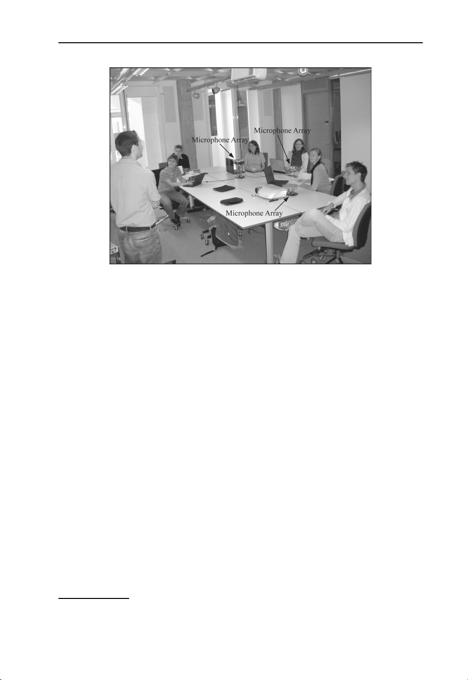
A typical meeting scenario as addressed by the AMIDA project is shown in Figure 1.1.
Note the three microphone arrays placed at various locations on the table, which are
intended to capture far-field speech for speaker tracking, beamforming, and DSR experiments. Although not shown in the photograph, the meeting participants typically also
wear close-talking microphones to provide the best possible sound capture as a reference
against which to judge the performance of the DSR system.
Page 21
Introduction 3
Figure 1.1 A typical AMIDA interaction. (© Photo reproduced by permission of the University
of Edinburgh)
1.1.2 Humanoid Robots
If humanoid robots are ever to be accepted as full ‘partners’ by their human users, they
must eventually develop perceptual capabilities similar to those possessed by humans, as
well as the capacity of performing a diverse collection of tasks, including learning, reasoning, communicating and forming goals through interaction with both users and instructors.
To provide for such capabilities, ASR is essential, because, as mentioned previously, spoken communication is the most common and flexible form of communication between
people. To provide a natural interaction between a human and a humanoid robot requires
not only the development of speech recognition systems capable of functioning reliably
on data captured with far-field sensors, but also natural language capabilities including a
sense of social interrelations and hierarchies.
In recent years, humanoid robots, albeit with very limited capabilities, have become
commonplace. They are, for example, deployed as entertainment or information systems.
Figure 1.2 shows an example of such a robot, namely, the humanoid tour guide robot
TPR-Robina
1
developed by Toyota. The robot is able to escort visitors around the Toyota Kaikan Exhibition Hall and to interact with them through a combination of verbal
communication and gestures.
While humanoid robots programmed for a limited range of tasks are already in
widespread use, such systems lack the capability of learning and adapting to new
environments. The development of such a capacity is essential for humanoid robots to
become helpful in everyday life. The Cognitive Systems for Cognitive Assistants (COSY)
project, financed by the European Union, has the objective to develops two kind of
robots providing such advanced capabilities. The first robot will find its way around a
1
ROBINA stands for ROBot as INtelligent Assistant.
Page 22
4 Distant Speech Recognition
Figure 1.2 Humanoid tour guide robot TPR-Robina by Toyota which escort visitors around Toyota
Kaikan Exhibition Hall in Toyota City, Aichi Prefecture, Japan. (© Photo reproduced by permission
of Toyota Motor Corporation)
complex building, showing others where to go and answering questions about routes
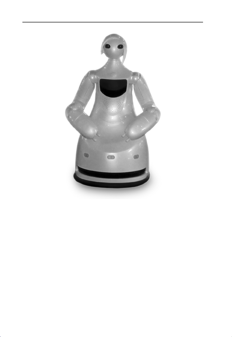
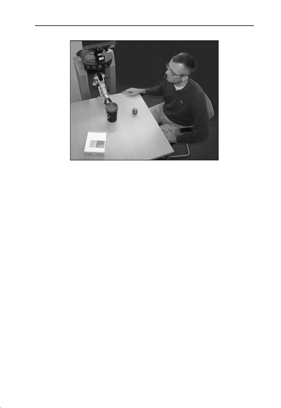
and locations. The second will be able to manipulate structured objects on a table top.
A photograph of the second COSY robot during an interaction session is shown in
Figure 1.3.
1.1.3 Automobiles
There is a growing trend in the automotive industry towards increasing both the number
and the complexity of the features available in high end models. Such features include
entertainment, navigation, and telematics systems, all of which compete for the driver’s
visual and auditory attention, and can increase his cognitive load. ASR in such automobile
environments would promote the “Eyes on the road, hands on the wheel” philosophy. This
would not only provide more convenience for the driver, but would in addition actually
Page 23
Introduction 5
Figure 1.3 Humanoid robot under development for the COSY project. (© Photo reproduced by
permission of DFKI GmbH)
enhance automotive safety. The enhanced safety is provided by hands-free operation of
everything but the car itself and thus would leave the driver free to concentrate on the
road and the traffic. Most luxury cars already have some sort of voice-control system
which are, for example, able to provide
• voice-activated, hands-free calling
Allows anyone in the contact list of the driver’s mobile phone to be called by voice
command.
• voice-activated music
Enables browsing through music using voice commands.
• audible information and text messages
Makes it possible to synthesize information and text messages, and have them read out
loud through speech synthesis.
This and other voice-controlled functionality will become available in the mass market
in the near future. An example of a voice-controlled car navigation system is shown in
Figure 1.4.
While high-end consumer automobiles have ever more features available, all of which
represent potential distractions from the task of driving the car, a police automobile has far
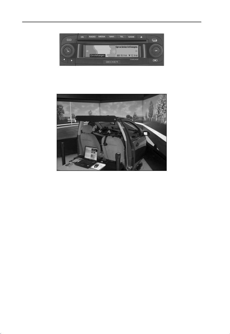
more devices that place demands on the driver’s attention. The goal of Project54 is to measure the cognitive load of New Hampshire state policeman – who are using speech-based
interfaces in their cars – during the course of their duties. Shown in Figure 1.5 is the
car simulator used by Project54 to measure the response times of police officers when
confronted with the task of driving a police cruiser as well as manipulating the several
devices contained therein through a speech interface.
Page 24
6 Distant Speech Recognition
Figure 1.4 Voice-controlled car navigation system by Becker. (© Photo reproduced by permission
of Herman/Becker Automotive Systems GmbH)
Figure 1.5 Automobile simulator at the University of New Hampshire. (© Photo reproduced by
permission of University of New Hampshire)
1.1.4 Speech-to-Speech Translation
Speech-to-speech translation systems provide a platform enabling communication with
others without the requirement of speaking or understanding a common language. Given
the nearly 6,000 different languages presently spoken somewhere on the Earth, and the
ever-increasing rate of globalization and frequency of travel, this is a capacity that will
in future be ever more in demand.
Even though speech-to-speech translation remains a very challenging task, commercial
products are already available that enable meaningful interactions in several scenarios. One
such system from National Telephone and Telegraph (NTT) DoCoMo of Japan works on a
common cell phone, as shown in Figure 1.6, providing voice-activated Japanese–English
and Japanese – Chinese translation. In a typical interaction, the user speaks short Japanese
phrases or sentences into the mobile phone. As the mobile phone does not provide
enough computational power for complete speech-to-text translation, the speech signal
is transformed into enhanced speech features which are transmitted to a server. The
server, operated by ATR-Trek, recognizes the speech and provides statistical translations,
which are then displayed on the screen of the cell-phone. The current system works
for both Japanese–English and Japanese– Chinese language pairs, offering translation in
Page 25

Introduction 7
Between Japanese and English
Between Japanese and Chinese
Figure 1.6 Cell phone, 905i Series by NTT DoCoMo, providing speech translation between
English and Japanese, and Chinese and Japanese developed by ATR and ATR-Trek. This service is
commercially available from NTT DoCoMo. (© Photos reproduced by permission of ATR-Trek)
both directions. For the future, however, preparation is underway to include support for
additional languages.
As the translations appear on the screen of the cell phone in the DoCoMo system, there
is a natural desire by users to hold the phone so that the screen is visible instead of next
to the ear. This would imply that the microphone is no longer only a few centimeters
from the mouth; i.e., we would have once more a distant speech recognition scenario.
Indeed, there is a similar trend in all hand-held devices supporting speech input.
Accurate translation of unrestricted speech is well beyond the capability of today’s
state-of-the-art research systems. Therefore, advances are needed to improve the
technologies for both speech recognition and speech translation. The development of
such technologies are the goals of the Technology and Corpora for Speech-to-Speech
Translation (TC-Star) project, financially supported by European Union, as well as the
Global Autonomous Language Exploitation (GALE) project sponsored by the DARPA.
These projects respectively aim to develop the capability for unconstrained conversational
speech-to-speech translation of English speeches given in the European Parliament, and
of broadcast news in Chinese or Arabic.
1.2 Challenges in Distant Speech Recognition
To guarantee high-quality sound capture, the microphones used in an ASR system should
be located at a fixed position, very close to the sound source, namely, the mouth of
the speaker. Thus body mounted microphones, such as head-sets or lapel microphones,
provide the highest sound quality. Such microphones are not practical in a broad variety
of situations, however, as they must be connected by a wire or radio link to a computer
and attached to the speaker’s body before the HCI can begin. As mentioned previously,
this makes HCI impractical in many situations where it would be most helpful; e.g., when
communicating with humanoid robots, or in intelligent room environments.
Although ASR is already used in several commercially available products, there are still
obstacles to be overcome in making DSR commercially viable. The two major sources
Page 26

8 Distant Speech Recognition
of degradation in DSR are distortions, such as additive noise and reverberation, and a
mismatch between training and test data , such as those introduced by speaking style
or accent. In DSR scenarios, the quality of the speech provided to the recognizer has a
decisive impact on system performance. This implies that speech enhancement techniques
are typically required to achieve the best possible signal quality.
In the last decades, many methods have been proposed to enable ASR systems to
compensate or adapt to mismatch due to interspeaker differences, articulation effects and
microphone characteristics. Today, those systems work well for different users on a broad
variety of applications, but only as long as the speech captured by the microphones is
free of other distortions. This explains the severe performance degradation encountered
in current ASR systems as soon as the microphone is moved away from the speaker’s
mouth. Such situations are known as distant, far-field or hands-free
2
speech recognition.
This dramatic drop in performance occurs mainly due to three different types of distortion:
3
• The first is noise, also known as background noise,
which is any sound other than the
desired speech, such as that from air conditioners, printers, machines in a factory, or
speech from other speakers.
• The second distortion is echo and reverberation, which are reflections of the sound
source arriving some time after the signal on the direct path.
• Other types of distortions are introduced by environmental factors such as room modes,
the orientation of the speaker’s head ,ortheLombard effect .
To limit the degradation in system performance introduced by these distortions, a great
deal of current research is devoted to exploiting several aspects of speech captured with
far-field sensors. In DSR applications, procedures already known from conventional ASR
can be adopted. For instance, confusion network combination is typically used with data
captured with a close-talking microphone to fuse word hypotheses obtained by using
various speech feature extraction schemes or even completely different ASR systems.
For DSR with multiple microphone conditions, confusion network combination can be
used to fuse word hypotheses from different microphones. Speech recognition with distant
sensors also introduces the possibility, however, of making use of techniques that were
either developed in other areas of signal processing, or that are entirely novel. It has
become common in the recent past, for example, to place a microphone array in the
speaker’s vicinity, enabling the speaker’s position to be determined and tracked with
time. Through beamforming techniques, a microphone array can also act as a spatial
filter to emphasize the speech of the desired speaker while suppressing ambient noise
or simultaneous speech from other speakers. Moreover, human speech has temporal,
spectral, and statistical characteristics that are very different from those possessed by
other signals for which conventional beamforming techniques have been used in the past.
Recent research has revealed that these characteristics can be exploited to perform more
effective beamforming for speech enhancement and recognition.
2
The latter term is misleading, inasmuch close-talking microphones are usually not held in the hand, but are
mounted to the head or body of the speaker.
3
This term is also misleading, in that the “background” could well be closer to the microphone than the “fore-
ground” signal of interest.
Page 27

Introduction 9
1.3 System Evaluation
Quantitative measures of the quality or performance of a system are essential for making
fundamental advances in the state-of-the-art. This fact is embodied in the often repeated
statement, “You improve what you measure.” In order to asses system performance, it is
essential to have error metrics or objective functions at hand which are well-suited to the
problem under investigation. Unfortunately, good objective functions do not exist for a
broad variety of problems, on the one hand, or else cannot be directly or automatically
evaluated, on the other.
Since the early 1980s, word error rate (WER) has emerged as the measure of first choice
for determining the quality of automatically-derived speech transcriptions. As typically
defined, an error in a speech transcription is of one of three types, all of which we will
now describe. A deletion occurs when the recognizer fails to hypothesize a word that
was spoken. An insertion occurs when the recognizer hypothesizes a word that was not
spoken. A substitution occurs when the recognizer misrecognizes a word. These three
errors are illustrated in the following partial hypothesis, where they are labeled with D,
I,andS, respectively:
Hyp: BUT ... WILL SELL THE CHAIN ... FOR EACH STORE SEPARATELY
Utt: ... IT WILL SELL THE CHAIN ... OR EACH STORE SEPARATELY
ID S
A more thorough discussion of word error rate is given in Section 14.1.
Even though widely accepted and used, word error rate is not without flaws. It has
been argued that the equal weighting of words should be replaced by a context sensitive
weighting, whereby, for example, information-bearing keywords should be assigned a
higher weight than functional words or articles. Additionally, it has been asserted that word
similarities should be considered. Such approaches, however, have never been widely
adopted as they are more difficult to evaluate and involve subjective judgment. Moreover,
these measures would raise new questions, such as how to measure the distance between
words or which words are important.
Naively it could be assumed that WER would be sufficient in ASR as an objective
measure. While this may be true for the user of an ASR system, it does not hold for the
engineer. In fact a broad variety of additional objective or cost functions are required.
These include:
• The Mahalanobis distance, which is used to evaluate the acoustic model.
• Perplexity, which is used to evaluate the language model as described in Section 7.3.1.
• Class separability , which is used to evaluate the feature extraction component or
front-end.
• Maximum mutual information or minimum phone error, which are used during discrim-
inate estimation of the parameters in a hidden Markov model.
• Maximum likelihood, which is the metric of first choice for the estimation of all system
parameters.
A DSR system requires additional objective functions to cope with problems not encoun-
tered in data captured with close-talking microphones. Among these are:
Page 28

10 Distant Speech Recognition
• Cross-correlation, which is used to estimate time delays of arrival between microphone
pairs as described in Section 10.1.
• Signal-to-noise ratio, which can be used for channel selection in a multiple-microphone
data capture scenario.
• Negentropy, which can be used for combining the signals captured by all sensors of a
microphone array.
Most of the objective functions mentioned above are useful because they show a significant correlation with WER. The performance of a system is optimized by minimizing or
maximizing a suitable objective function. The way in which this optimization is conducted
depends both on the objective function and the nature of the underlying model. In the best
case, a closed-form solution is available, such as in the optimization of the beamforming
weights as discussed in Section 13.3. In other cases, an iterative solution can be adopted,
such as when optimizing the parameters of a hidden Markov model (HMM) as discussed
in Chapter 8. In still other cases, numerical optimization algorithms must be used such
as when optimization the parameters of an all-pass transform for speaker adaptation as
discussedinSection9.2.2.
To chose the appropriate objective function a number of decisions must be made
(H¨ansler and Schmidt 2004, sect. 4):
• What kind of information is available?
• How should the available information be used?
• How should the error be weighted by the objective function?
• Should the objective function be deterministic or stochastic?
Throughout the balance of this text, we will strive to answer these questions whenever
introducing an objective function for a particular application or in a particular context.
When a given objective function is better suited than another for a particular purpose, we
will indicate why. As mentioned above, the reasoning typically centers around the fact
that the better suited objective function is more closely correlated with word error rate.
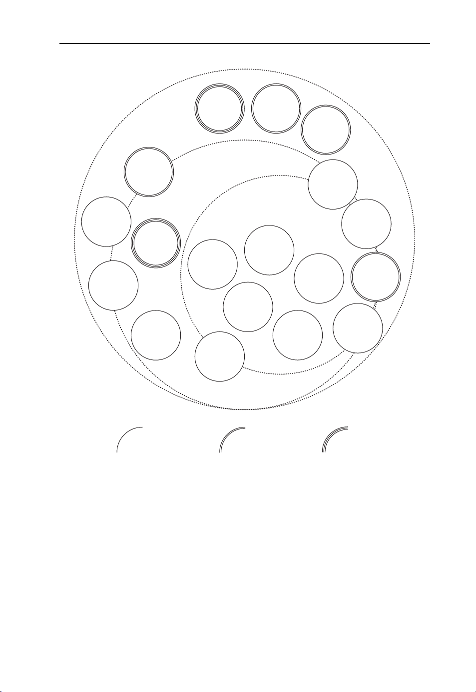
1.4 Fields of Speech Recognition
Figure 1.7 presents several subtopics of speech recognition in general which can be
associated with three different fields: automatic, robust and distant speech recognition.
While some topics such as multilingual speech recognition and language modeling can
be clearly assigned to one group (i.e., automatic) other topics such as feature extraction
or adaptation cannot be uniquely assigned to a single group. A second classification of
topics shown in Figure 1.7 depends on the number and type of sensors. Whereas one
microphone is traditionally used for recognition, in distant recognition the traditional
sensor configuration can be augmented by an entire array of microphones with known or
unknown geometry. For specific tasks such as lipreading or speaker localization, additional
sensor types such as video cameras can be used.
Undoubtedly, the construction of optimal DSR systems must draw on concepts from
several fields, including acoustics, signal processing, pattern recognition, speaker tracking
and beamforming. As has been shown in the past, all components can be optimized
Page 29
Introduction 11
dereverberation
feature
enhancement
distant speech
recognition
blind
source
separation
lip reading
missing
features
localization
and
tracking
robust speech
recognition
automatic speech
search
linguistics
adaptation
beamforming
recognition
multi
lingual
modeling
language
modeling
channel
selection
feature
extraction
acoustic
uncertainty
decoding
channel
combination
acoustics
single microphone multi microphone multi sensor
Figure 1.7 Illustration of the different fields of speech recognition: automatic, robust and distant
separately to construct a DSR system. Such an independent treatment, however, does
not allow for optimal performance. Moreover, new techniques have recently emerged
exploiting the complementary effects of the several components of a DSR system. These
include:
• More closely coupling the feature extraction and acoustic models; e.g., by propagating
the uncertainty of the feature extraction into the HMM.
• Feeding the word hypotheses produced by the DSR back to the component located
earlier in the processing chain; e.g. by feature enhancement with particle filters with
models for different phoneme classes.
Page 30

12 Distant Speech Recognition
• Replacing traditional objective functions such as signal-to-noise ratio by objective
functions taking into account the acoustic model of the speech recognition system,
as in maximum likelihood beamforming, or considering the particular characteristics of
human speech, as in maximum negentropy beamforming.
1.5 Robust Perception
In contrast to automatic pattern recognition, human perception is very robust in the
presence of distortions such as noise and reverberation. Therefore, knowledge of the
mechanisms of human perception, in particular with regard to robustness, may also be
useful in the development of automatic systems that must operate in difficult acoustic
environments. It is interesting to note that the cognitive load for humans increases while
listening in noisy environments, even when the speech remains intelligible (Kjellberg
et al. 2007). This section presents some illustrative examples of human perceptual
phenomena and robustness. We also present several technical solutions based on these
phenomena which are known to improve robustness in automatic recognition.
1.5.1 A Priori Knowledge
When confronted with an ambiguous stimulus requiring a single interpretation, the human
brain must rely on apriori knowledge and expectations. What is likely to be one of the
most amazing findings about the robustness and flexibility of human perception and the
use of apriori information is illustrated by the following sentence, which was circulated
in the Internet in September 2003:
Aoccdrnig to rscheearch at Cmabrigde uinervtisy, it deosn’t mttaer waht oredr the
ltteers in a wrod are, the olny ipromoetnt tihng is taht the frist and lsat ltteres are
at the rghit pclae. The rset can be a tatol mses and you can sitll raed it wouthit a
porbelm. Tihs is bcuseae we do not raed ervey lteter by itslef but the wrod as a
wlohe.
The text is easy to read for a human inasmuch as, through reordering, the brain maps
the erroneously presented characters into correct English words.
Apriori knowledge is also widely used in automatic speech processing. Obvious
examples are
• the statistics of speech,
• the limited number of possible phoneme combinations constrained by known words
which might be further constrained by the domain,
• the word sequences follow a particular structure which can be represented as a context
free grammar or the knowledge of successive words, represented as an N-gram .
1.5.2 Phonemic Restoration and Reliability
Most signals of interest, including human speech, are highly redundant. This redundancy
provides for correct recognition or classification even in the event that the signal is partially
Page 31

Introduction 13
Figure 1.8 Adding a mask to the occluded portions of the top image renders the word legible, as
is evident in the lower image
occluded or otherwise distorted, which implies that a significant amount of information is
missing. The sophisticated capabilities of the human brain underlying robust perception
were demonstrated by Fletcher (1953), who found that verbal communication between
humans is possible if either the frequencies below or above 1800 Hz are filtered out.
An illusory phenomenon, which clearly illustrates the robustness of the human auditory
system, is known as the phonemic restoration effect, whereby phonetic information that
is actually missing in a speech signal can be synthesized by the brain and clearly heard
(Miller and Licklider 1950; Warren 1970). Furthermore, the knowledge of which information is distorted or missing can significantly improve perception. For example, knowledge
about the occluded portion of an image can render a word readable, as is apparent upon
considering Figure 1.8. Similarly, the comprehensibility of speech can be improved by
adding noise (Warren et al. 1997).
Several problems in automatic data processing – such as occlusion – which were first
investigated in the context of visual pattern recognition, are now current research topics
in robust speech recognition. One can distinguish between two related approaches for
coping with this problem:
• missing feature theory
In missing feature theory, unreliable information is either ignored, set to some fixed
nominal value, such as the global mean, or interpolated from nearby reliable infor-
mation. In many cases, however, the restoration of missing features by spectral and/or
temporal interpolation is less effective than simply ignoring them. The reason for this is
that no processing can re-create information that has been lost as long as no additional
information, such as an estimate of the noise or its propagation, is available.
• uncertainty processing
In uncertainty processing, unreliable information is assumed to be unaltered, but the
unreliable portion of the data is assigned less weight than the reliable portion.
Page 32

14 Distant Speech Recognition
1.5.3 Binaural Masking Level Difference
Even though the most obvious benefit from binaural hearing lies in source localization,
other interesting effects exist: If the same signal and noise is presented to both ears with
a noise level so high as to mask the signal, the signal is inaudible. Paradoxically, if either
of the two ears is unable to hear the signal, it becomes once more audible. This effect is
known as the binaural masking level difference. The binaural improvements in observing
a signal in noise can be up to 20 dB (Durlach 1972). As discussed in Section 6.9.1, the
binaural masking level difference can be related to spectral subtraction, wherein two input
signals, one containing both the desired signal along with noise, and the second containing
only the noise, are present. A closely related effect is the so-called cocktail party effect
(Handel 1989), which describes the capacity of humans to suppress undesired sounds,
such as the babble during a cocktail party, and concentrate on the desired signal, such as
the voice of a conversation partner.
1.5.4 Multi-Microphone Processing
The use of multiple microphones is motivated by nature, in which two ears have been
shown to enhance speech understanding as well as acoustic source localization. This effect
is even further extended for a group of people, where one person could not understand
some words, a person next to the first might have and together they are able to understand
more than independent of each other.
Similarly, different tiers in a speech recognition system, which are derived either from
different channels (e.g., microphones at different locations or visual observations) or
from the variance in the recognition system itself, produce different recognition results.
An appropriate combination of the different tiers can improve recognition performance.
The degree of success depends on
• the variance of the information provided by the different tiers,
• the quality and reliability of the different tiers and
• the method used to combine the different tiers.
In automatic speech recognition, the different tiers can be combined at various stages of
the recognition system providing different advantages and disadvantages:
• signal combination
Signal-based algorithms, such as beamforming, exploit the spatial diversity resulting
from the fact that the desired and interfering signal sources are in practice located at
different points in space. These approaches assume that the time delays of the signals
between different microphone pairs are known or can be reliably estimated. The spatial
diversity can then be exploited by suppressing signals coming from directions other
than that of the desired source.
• feature combination
These algorithms concatenate features derived by different feature extraction methods
to form a new feature vector. In such an approach, it is a common practice to reduce
the number of features by principal component analysis or linear discriminant analysis.
Page 33

Introduction 15
While such algorithms are simple to implement, they suffer in performance if the
different streams are not perfectly synchronized.
• word and lattice combination
Those algorithms, such as recognizer output voting error reduction (ROVER) and confusion network combination, combine the information of the recognition output which
can be represented as a first best, N-best or lattice word sequence and might be augmented with a confidence score for each word.
In the following we present some examples where different tiers have been successfully combined: Stolcke et al. (2005) used two different front-ends, mel-frequency cepstral
coefficients and features derived from perceptual linear prediction, for cross-adaptation
and system combination via confusion networks. Both of these features are described in
Chapter 5. Yu et al. (2004) demonstrated, on a Chinese ASR system, that two different
kinds of models, one on phonemes, the other on semi-syllables, can be combined to good
effect. Lamel and Gauvain (2005) combined systems trained with different phoneme sets
using ROVER. Siohan et al. (2005) combined randomized decision trees. St¨uker et al.
(2006) showed that a combination of four systems – two different phoneme sets with two
feature extraction strategies – leads to additional improvements over the combination of
two different phoneme sets or two front-ends. St¨uker et al. also found that combining
two systems, where both the phoneme set and front-ends are altered, leads to improved
recognition accuracy compared to changing only the phoneme set or only the front-end.
This fact follows from the increased variance between the two different channels to be
combined. The previous systems have combined different tiers using only a single channel combination technique. W¨olfel et al. (2006) demonstrated that a hybrid approach
combining the different tiers, derived from different microphones, at different stages in a
distant speech recognition system leads to additional improvements over a single combination approach. In particular W¨olfel et al. achieved fewer recognition errors by using a
combination of beamforming and confusion network.
1.5.5 Multiple Sources by Different Modalities
Given that it often happens that no single modality is powerful enough to provide correct
classification, one of the key issues in robust human perception is the efficient merging
of different input modalities, such as audio and vision, to render a stimulus intelligible
(Ernst and B¨ulthoff 2004; Jacobs 2002). An illustrative example demonstrating the multimodality of speech perception is the McGurk effect
which is experienced when contrary audiovisual information is presented to human subjects. To wit, a video presenting a visual /ga/ combined with an audio /ba/ will be
perceived by 98% of adults as the syllable /da/. This effect exists not only for single
syllables, but can alter the perception of entire spoken utterances, as was confirmed by
a study about witness testimony (Wright and Wareham 2005). It is interesting to note
that awareness of the effect does not change the perception. This stands in stark contrast
to certain optical illusions, which are destroyed as soon as the subject is aware of the
deception.
4
This is often referred to as the McGurk – MacDonald effect.
4
(McGurk and MacDonald 1976),
Page 34

16 Distant Speech Recognition
Humans follow two different strategies to combine information:
• maximizing information (sensor combination)
If the different modalities are complementary, the various pieces of information about
an object are combined to maximize the knowledge about the particular observation.
For example, consider a three-dimensional object, the correct recognition of which
is dependent upon the orientation of the object to the observer. Without rotating the
object, vision provides only two-dimensional information about the object, while the
5
haptic
input provides the missing three-dimensional information (Newell 2001).
• reducing variance (sensor integration)
If different modalities overlap, the variance of the information is reduced. Under the
independence and Gaussian assumption of the noise, the estimate with the lowest variance is identical to the maximum likelihood estimate.
One example of the integration of audio and video information for localization supporting the reduction in variance theory is given by Alais and Burr (2004).
Two prominent technical implementations of sensor fusion are audio-visual speaker
tracking, which will be presented in Section 10.4, and audio-visual speech recognition. A
good overview paper of the latter is by Potamianos et al. (2004).
1.6 Organizations, Conferences and Journals
Like all other well-established scientific disciplines, the fields of speech processing and
recognition have founded and fostered an elaborate network of conferences and publications. Such networks are critical for promoting and disseminating scientific progress in
the field. The most important organizations that plan and hold such conferences on speech
processing and publish scholarly journals are listed in Table 1.1.
At conferences and in their associated proceedings the most recent advances in the
state-of-the-art are reported, discussed, and frequently lead to further advances. Several
major conferences take place every year or every other year. These conferences are listed
in Table 1.2. The principal advantage of conferences is that they provide a venue for
Table 1.1 Organizations promoting research in speech processing and recognition
Abbreviation Full Name
IEEE Institute of Electrical and Electronics Engineers
ISCA International Speech Communication Association former
European Speech Communication Association (ESCA)
EURASIP European Association for Signal Processing
ASA Acoustical Society of America
ASJ Acoustical Society of Japan
EAA European Acoustics Association
5
Haptic phenomena pertain to the sense of touch.
Page 35

Introduction 17
Table 1.2 Speech processing and recognition conferences
Abbreviation Full Name
ICASSP International Conference on Acoustics, Speech, and Signal Processing by IEEE
Interspeech ISCA conference; previous Eurospeech and International Conference on
Spoken Language Processing (ICSLP)
ASRU Automatic Speech Recognition and Understanding by IEEE
EUSIPCO European Signal Processing Conference by EURASIP
HSCMA Hands-free Speech Communication and Microphone Arrays
WASPAA Workshop on Applications of Signal Processing to Audio and Acoustics
IWAENC International Workshop on Acoustic Echo and Noise Control
ISCSLP International Symposium on Chinese Spoken Language Processing
ICMI International Conference on Multimodal Interfaces
MLMI Machine Learning for Multimodal Interaction
HLT Human Language Technology
the most recent advances to be reported. The disadvantage of conferences is that the
process of peer review by which the papers to be presented and published are chosen
is on an extremely tight time schedule. Each submission is either accepted or rejected,
with no time allowed for discussion with or clarification from the authors. In addition
to the scientific papers themselves, conferences offer a venue for presentations, expert
panel discussions, keynote speeches and exhibits, all of which foster further scientific
progress in speech processing and recognition. Information about individual conferences
is typically disseminated in the Internet. For example, to learn about the Workshop on
Applications of Signal Processing to Audio and Acoustics, which is to be held in 2009, it
is only necessary to type waspaa 2009 into an Internet search window.
Journals differ from conferences in two ways. Firstly, a journal offers no chance for
the scientific community to gather regularly at a specific place and time to present and
discuss recent research. Secondly and more importantly, the process of peer review for
an article submitted for publication in a journal is far more stringent than that for any
conference. Because there is no fixed time schedule for publication, the reviewers for
a journal can place far more demands on authors prior to publication. They can, for
example, request more graphs or figures, more experiments, further citations to other
scientific work, not to mention improvements in English usage and overall quality of
presentation. While all of this means that greater time and effort must be devoted to
the preparation and revision of a journal publication, it is also the primary advantage of
journals with respect to conferences. The dialogue that ensues between the authors and
reviewers of a journal publication is the very core of the scientific process. Through the
succession of assertion, rebuttal, and counter assertion, non-novel claims are identified
and withdrawn, unjustifiable claims are either eliminated or modified, while the arguments for justifiable claims are strengthened and clarified. Moreover, through the act of
publishing a journal article and the associated dialogue, both authors and reviewers typically learn much they had not previously known. Table 1.3 lists several journals which
cover topics presented in this book and which are recognized by academia and industry
alike.
Page 36

18 Distant Speech Recognition
Table 1.3 Speech processing and recognition journals
Abbreviation Full name
SP IEEE Transactions on Signal Processing
ASLP IEEE Transactions on Audio, Speech and Language Processing former IEEE
Transactions on Speech and Audio Processing (SAP)
ASSP IEEE Transactions on Acoustics, Speech and Signal Processing
SPL IEEE Signal Processing Letters
SPM IEEE Signal Processing Magazine
CSL Computer Speech and Language by Elsevier
ASA Journal of the Acoustic Society of America
SP EURASIP Journal on Signal Processing
AdvSP EURASIP Journal on Advances in Signal Processing
SC EURASIP and ISCA Journal on Speech Communication published by Elsevier
AppSP EURASIP Journal on Applied Signal Processing
ASMP EURASIP Journal on Audio, Speech and Music Processing
An updated list of conferences, including a calendar of upcoming events, and journals
can be found on the companion website of this book at
http://www.distant-speech-recognition.org
1.7 Useful Tools, Data Resources and Evaluation Campaigns
A broad number of commercial and non-commercial tools are available for the processing,
analysis and recognition of speech. An extensive and updated list of such tools can be
found on the companion website of this book.
The right data or corpora is essential for training and testing various speech processing,
enhancement and recognition algorithms. This follows from the fact that the quality of
the acoustic and language models are determined in large part by the amount of available
training data, and the similarity between the data used for training and testing. As collecting and transcribing appropriate data is time-consuming and expensive, and as reporting
WER reductions on “private” data makes the direct comparison of techniques and systems
difficult or impossible, it is highly worth-while to report experimental results on publicly
available speech corpora whenever possible. The goal of evaluation campaigns, such as
the Rich Transcription (RT) evaluation staged periodically by the US National Institute
of Standards and Technologies (NIST), is to evaluate and to compare different speech
recognition systems and the techniques on which they are based. Such evaluations are
essential in order to assess not only the progress of individual systems, but also that of
the field as a whole. Possible data sources and evaluation campaigns are listed on the
website mentioned previously.
1.8 Organization of this Book
Our aim in writing this book was to provide in a single volume an exposition of the theory
behind each component of a complete DSR system. We now summarize the remaining
Page 37

Introduction 19
Sensors
Perceptual Components
Audio
Features
Video
Features
Automatic Speech Recognition
Dictionary
Output
Language
Adaptation
9
Model
Channel
Selection
Blind Source
12 13
Separation
Acoustic
Model
Adaptation
Speaker
1012
Tracking
Beamforming
Segmentation
Clustering
Feature
5
Extraction
Feature
6
Enhancement
Adaptation
Search
7
Text Location
Figure 1.9 Architecture of a distant speech recognition system. The gray numbers indicate the
corresponding chapter of this book
contents of this volume in order to briefly illustrate both the narrative thread that underlies
this work, as well as the interrelations among the several chapters. In particular, we will
emphasize how the development of each chapter is prefigured by and builds upon that
of the preceding chapters. Figure 1.9 provides a high-level overview of a DSR system
following the signal flow through the several components. The gray number on each
individual component indicates the corresponding chapter in this book. The chapters not
shown in the figure, in particular Chapters 2, 3, 4, 8 and 11, present material necessary
to support the development in the other chapters: The fundamentals of sound propagation
and acoustics are presented in Chapter 2, as are the basics of speech production. Chapter 3
presents linear filtering techniques that are used throughout the text. Chapter 4 presents the
theory of Bayesian filters, which will later be applied both for speech feature enhancement
Page 38

20 Distant Speech Recognition
in Chapter 6 and speaker tracking in Chapter 10. Chapter 8 discusses how the parameters
of a HMM can be reliably estimated based on the use of transcribed acoustic data. Such
a HMM is an essential component of most current DSR systems, in that it extracts word
hypotheses from the final waveform produced by the other components of the system.
Chapter 11 provides a discussion of digital filter banks, which, as discussed in Chapter 13,
are an important component of a beamformer. Finally, Chapter 14 reports experimental
results indicating the effectiveness of the algorithms described throughout this volume.
Speech, like any sound, is the propagation of pressure waves through air or any other
liquid. A DSR system extracts from such pressure waves hypotheses of the phonetic units
and words uttered by a speaker. Hence, it is worth-while to understand the physics of sound
propagation, as well as how the spectral and temporal characteristics of speech are altered
when it is captured by far-field sensors in realistic acoustic environments. These topics
are considered in Chapter 2. This chapter also presents the characteristics and properties
of the human auditory system. Knowledge of the latter is useful, inasmuch as experience
has shown that many insights gained from studying the human auditory system have been
successfully applied to improve the performance of automatic speech recognition systems.
In signal processing, the term filter refers to an algorithm which extracts a desired signal from an input signal corrupted by noise or other distortions. A filter can also be used
to modify the spectral or temporal characteristics of a signal in some advantageous way.
Therefore, filtering techniques are powerful tools for speech signal processing and distant
recognition. Chapter 3 provides a review of the basics of digital signal processing, including a short introduction to linear time-invariant systems, the Fourier and z-transforms, as
well as the effects of sampling and reconstruction. Next there is a presentation of the
discrete Fourier transform and its use for the implementation of linear time-invariant systems, which is followed by a description of the short-time Fourier transform. The contents
of this chapter will be referred to extensively in Chapter 5 on speech feature extraction,
as well as in Chapter 11 on digital filter banks.
Many problems in science and engineering can be formulated as the estimation of some
state, which cannot be observed directly, based on a series of features or observations,
which can be directly observed. The observations are often corrupted by distortions such
as noise or reverberation. Such problems can be solved with one of a number of Bayesian
filters, all of which estimate an unobservable state given a series of observations. Chapter 4
first formulates the general problem to be solved by a Bayesian filter, namely, tracking the
likelihood of the state as it evolves in time as conditioned on a sequence of observations.
Thereafter, it presents several different solutions to this general problem, including the
classic Kalman filter and its variants, as well as the class of particle filters, which have
much more recently appeared in the literature. The theory of Bayesian filters will be
applied in Chapter 6 to the task of enhancing speech features that have been corrupted by
noise, reverberation or both. A second application, that of tracking the physical position
of a speaker based on the signals captured with the elements of a microphone array, will
be discussed in Chapter 10.
Automatic recognition requires that the speech waveform is processed so as to produce feature vectors of a relatively small dimension. This reduction in dimensionality
is necessary in order to avoid wasting parameters modeling characteristics of the signal
which are irrelevant for classification. The transformation of the input data into a set
of dimension-reduced features is called speech feature extraction, acoustic preprocessing
Page 39

Introduction 21
or front-end processing. As explained in Chapter 5, feature extraction in the context of
DSR systems aims to preserve the information needed to distinguish between phonetic
classes, while being invariant to other factors. The latter include speaker differences,
such as accent, emotion or speaking rate, as well as environmental distortions such as
background noise, channel differences, or reverberation.
The principle underlying speech feature enhancement, the topic of Chapter 6, is the
estimation of the original features of the clean speech from a corrupted signal. Usually
the enhancement takes place either in the power, logarithmic spectral or cepstral domain.
The prerequisite for such techniques is that the noise or the impulse response is known or
can be reliably estimated in the cases of noise or channel distortion, respectively. In many
applications only a single channel is available and therefore the noise estimate must be
inferred directly from the noise-corrupted signal. A simple method for accomplishing this
separates the signal into speech and non-speech regions, so that the noise spectrum can be
estimated from those regions containing no speech. Such simple techniques, however, are
not able to cope well with non-stationary distortions. Hence, more advanced algorithms
capable of actively tracking changes in the noise and channel distortions are the main
focus of Chapter 6.
As discussed in Chapter 7, search is the process by which a statistical ASR system finds
the most likely word sequence conditioned on a sequence of acoustic observations. The
search process can be posed as that of finding the shortest path through a search graph.
The construction of such a search graph requires several knowledge sources, namely, a
language model, a word lexicon, and a HMM, as well as an acoustic model to evaluate the
likelihoods of the acoustic features extracted from the speech to be recognized. Moreover,
inasmuch as all human speech is affected by coarticulation, a decision tree for representing context dependency is required in order to achieve state-of-the-art performance. The
representation of these knowledge sources as weighted finite-state transducers is also presented in Chapter 7, as are weighted composition and a set of equivalence transformations,
including determinization, minimization, and epsilon removal. These algorithms enable
the knowledge sources to be combined into a single search graph, which can then be
optimized to provide maximal search efficiency.
All ASR systems based on the HMM contain an enormous number of free parameters.
In order to train these free parameters, dozens if not hundreds or even thousands of hours
of transcribed acoustic data are required. Parameter estimation can then be performed
according to either a maximum likelihood criterion or one of several discriminative criteria
such as maximum mutual information or minimum phone error. Algorithms for efficiently
estimating the parameters of a HMM are the subjects of Chapter 8. Included among
these are a discussion of the well-known expectation-maximization algorithm, with which
maximum likelihood estimation of HMM parameters is almost invariably performed.
Several discriminative optimization criteria, namely, maximum mutual information, and
minimum word and phone error are also described.
The unique characteristics of the voice of a particular speaker are what allow a person
calling on the telephone to be identified as soon as a few syllables have been spoken.
These characteristics include fundamental frequency, speaking rate, and accent, among
others. While lending each voice its own individuality and charm, such characteristics are
a hindrance to automatic recognition, inasmuch as they introduce variability in the speech
that is of no use in distinguishing between different words. To enhance the performance
Page 40

22 Distant Speech Recognition
of an ASR system that must function well for any speaker as well as different acoustic
environments, various transformations are typically applied either to the features, the
means and covariances of the acoustic model, or to both. The body of techniques used to
estimate and apply such transformations fall under the rubrik feature and model adaptation
and comprise the subject matter of Chapter 9.
While a recognition engine is needed to convert waveforms into word hypotheses, the
speech recognizer by itself is not the only component of a distant recognition system.
In Chapter 10, we introduce an important supporting technology required for a complete
DSR system, namely, algorithms for determining the physical positions of one or more
speakers in a room, and tracking changes in these positions with time. Speaker localization
and tracking – whether based on acoustic features, video features, or both – are important
technologies, because the beamforming algorithms discussed in Chapter 13 all assume that
the position of the desired speaker is known. Moreover, the accuracy of a speaker tracking
system has a very significant influence on the recognition accuracy of the entire system.
Chapter 11 discusses digital filter banks, which are arrays of bandpass filters that separate an input signal into many narrowband components. As mentioned previously, frequent
reference will be made to such filter banks in Chapter 13 during the discussion of beamforming. The optimal design of such filter banks has a critical effect on the final system
accuracy.
Blind source separation (BSS) and independent component analysis (ICA) are terms
used to describe classes of techniques by which signals from multiple sensors may be combined into one signal. As presented in Chapter 12, this class of methods is known as blind
because neither the relative positions of the sensors, nor the position of the sources are
assumed to be known. Rather, BSS algorithms attempt to separate different sources based
only on their temporal, spectral, or statistical characteristics. Most information-bearing signals are non-Gaussian, and this fact is extremely useful in separating signals based only
on their statistical characteristics. Hence, the primary assumption of ICA is that interesting
signals are not Gaussian signals. Several optimization criteria that are typically applied in
the ICA field include kurtosis, negentropy, and mutual information. While mutual information can be calculated for both Gaussian and non-Gaussian random variables alike,
kurtosis and negentropy are only meaningful for non-Gaussian signals. Many algorithms
for blind source separation, dispense with the assumption of non-Gaussianity and instead
attempt to separate signals on the basis of their non-stationarity or non-whiteness. Insights
from the fields of BSS and ICA will also be applied to good effect in Chapter 13 for
developing novel beamforming algorithms.
Chapter 13 presents a class of techniques, known collectively as beamforming, by
which signals from several sensors can be combined to emphasize a desired source and to
suppress all other noise and interference. Beamforming begins with the assumption that
the positions of all sensors are known, and that the positions of the desired sources are
known or can be estimated. The simplest of beamforming algorithms, the delay-and-sum
beamformer, uses only this geometrical knowledge to combine the signals from several
sensors. More sophisticated adaptive beamformers attempt to minimize the total output
power of an array of sensors under a constraint that the desired source must be unattenuated. Recent research has revealed that such optimization criteria used in conventional
array processing are not optimal for acoustic beamforming applications. Hence, Chapter
Page 41

Introduction 23
13 also presents several nonconventional beamforming algorithms based on optimization
criteria – such as mutual information, kurtosis, and negentropy – that are typically used
in the fields of BSS or ICA.
In the final chapter of this volume we present the results of performance evaluations of
the algorithms described here on several DSR tasks. These include an evaluation of the
speaker tracking component in isolation from the rest of the DSR system. In Chapter 14,
we present results illustrating the effectiveness of single-channel speech feature enhancement based on particle filters. Also included are experimental results for systems based
on beamforming for both single distant speakers, as well as two simultaneously active
speakers. In addition, we present results illustrating the importance of selecting a filter
bank suitable for adaptive filtering and beamforming when designing a complete DSR
system.
A note about the brevity of the chapters mentioned above is perhaps now in order. To
wit, each of these chapters might easily be expanded into a book much larger than the
present volume. Indeed, such books are readily available on sound propagation, digital
signal processing, Bayesian filtering, speech feature extraction, HMM parameter estimation, finite-state automata, blind source separation, and beamforming using conventional
criteria. Our goal in writing this work, however, was to create an accessible description
of all the components of a DSR system required to transform sound waves into word
hypotheses, including metrics for gauging the efficacy of such a system. Hence, judicious selection of the topics covered along with concise presentation were the criteria that
guided the choice of every word written here. We have, however, been at pains to provide
references to lengthier specialized works where applicable – as well as references to the
most relevant contributions in the literature – for those desiring a deeper knowledge of
the field. Indeed, this volume is intended as a starting point for such wider exploration.
1.9 Principal Symbols used Throughout the Book
This section defines principal symbols which are used throughout the book. Due to the
numerous variables each chapter presents an individual list of principal symbols which is
specific for the particular chapter.
Symbol Description
a, b, c, . . . variables
A, B, C, . . . constants
a, b, c, A, B, C,... units
a, b, c,... vectors
A, B, C,... matrices
I unity matrix
j imaginary number,
∗
·
complex conjungate
√
−1
Page 42

24 Distant Speech Recognition
Symbol Description
T
·
·
·
∇
H
1:K
2
transpose operator
Hermetian operator
sequence from 1 to K
Laplace operator
· average
˜· warped frequency
ˆ· estimate
% modulo
λ Lagrange multiplier
(·)
E{·
+
}
pseudoinverse of(·
expectation value
)
/ · / denote a phoneme
[·] denote a phone
|·| absolute (scalar) or determinant (matrix)
μ mean
covariance matrix
N (x;μ, ) Gaussian distribution with mean vector μ and covariance
matrix
∀ for all
∗ convolution
δ Dirac impulse
O big O notation also called Landau notation
C complex number
N set of natural numbers
N
0
set of non-negative natural numbers including zero
R real number
+
R
non-negative real number
Z integer number
+
Z
sinc(z)
non-negative integer number
1, for z = 0,
sin(z)/z, otherwise
Page 43

Introduction 25
1.10 Units used Throughout the Book
This section defines units that are consistently defined throughout the book.
Units Description
Hz Herz
J Joule
KKelvin
Pa Pascal
SPL sound pressure level
2
Vs/m
WWatt
◦
C degree Celsius
dB decibel
kg kilogram
mmeter
2
m
3
m
m/s velocity
s second
Tesl a
square meter
cubic meter
Page 44

2
Acoustics
The acoustical environment and the recording sensor configuration define the characteristics of distant speech recordings and thus the usability of the data for certain applications,
techniques or investigations. The scope of this chapter is to describe the physical aspect
of sound and the characteristics of speech signals. In addition, we will discuss the human
perception of sound, as well as the acoustic environment typically encountered in distant
speech recognition scenarios. Moreover, there will be a presentation of recording techniques and possible sensor configurations for use in the capture of sound for subsequent
distant speech recognition experiments.
The balance of this chapter is organized as follows. In Section 2.1, the physics of
sound production are presented. This includes a discussion of the reduction in sound
intensity that increases with the distance from the source, as well as the reflections
that occur at surfaces. The characteristics of human speech and its production are
described in Section 2.2. The subword units or phonemes of which human languages
are composed are also presented in Section 2.2. The human perception of sound, along
with the frequency-dependent sensitivity of the human auditory system, is described in
Section 2.3. The characteristics of sound propagation in realistic acoustic environments
is described in Section 2.4. Especially important in this section is the description of
the spectral and temporal changes that speech and other sounds undergo when they
propagate through enclosed spaces. Techniques and best practices for sound capture and
recording are presented in Section 2.5. The final section summarizes the contents of this
chapter and presents suggestions for further reading.
2.1 Physical Aspect of Sound
The physical – as opposed to perceptual – properties of sound can be characterized as the
superposition of waves of different pressure levels which propagate through compressible
media such as air. Consider, for example, one molecule of air which is accelerated and
displaced from its original position. As it is surrounded by other molecules, it bounces into
those adjacent, imposing a force in the opposite direction which causes the molecule to
recoil and to return to its original position. The transmitted force accelerates and displaces
the adjacent molecules from their original position which once more causes the molecules
Distant Speech Recognition Matthias W¨olfel and John McDonough
© 2009 John Wiley & Sons, Ltd. ISBN: 978-0-470-51704-8
Page 45

28 Distant Speech Recognition
to bounce into other adjacent molecules. Therefore, the molecules undergo movements
around their mean positions in the direction of propagation of the sound wave. Such
behavior is known as a longitudinal wave. The propagation of the sound wave cause the
molecules which are half a wavelength apart from each other to vibrate with opposite
phase and thus produce alternate regions of compression and rarefaction. It follows that
the sound pressure, defined as the difference between the instantaneous pressure and the
static pressure, is a function of position and time.
Our concern here is exclusively with the propagation of sound in air and we assume
the media of propagation to be homogeneous, which implies it has a uniform structure,
isotropic, which implies its properties are the same in all directions, and stationary ,which
implies these properties do not change with time. These assumptions are not entirely
justified, but the effects due to inhomogeneous and non-stationary media are negligible
in comparison with those to be discussed; hence, so they can be effectively ignored.
2.1.1 Propagation of Sound in Air
Media capable of sound transfer have two properties, namely, mass and elasticity. The
elasticity of an ideal gas is defined by its volume dilatation and volume compression.
The governing relation of an ideal gas, given a specific gas constant R, is defined by the
state equation
V
p
= R, (2.1)
M
where p denotes the pressure, commonly measured in Pascal (Pa), V the volume com-
3
monly measured in cubic meters (m
(kg), and the temperature commonly measured in degrees Kelvin (K).
specific gas constant is R
dryair
), M the mass , commonly measured in kilograms
1
For dry air the
= 287.05 J/(kg · K) where J represents Joule. Air at sea
level and room temperature is well-modeled by the state equation (2.1). Thus, we will
treat air as an ideal gas for the balance of this book.
The volume compression,ornegative dilatation , of an ideal gas is defined as
− −
δV
V
,
where V represents the volume at the initial state and δV represents the volume variation.
The elasticity of an ideal gas is determined by the bulk modulus
δp
−
,
κ
which is defined as the ratio between the pressure variation δp and the volume compression. An adiabatic process is a thermodynamic process in which no heat is transferred to
or from the medium. Sound propagation is adiabatic because the expansions and contractions of a longitudinal wave occur very rapidly with respect to any heat transfer. Let C
1
Absolute zero is 0 K ≈−273.15◦C. No substance can be colder than this.
p
Page 46

Acoustics 29
and Cvdenote the specific heat capacities under constant pressure and constant volume,
respectively. Given the adiabatic nature of sound propagation, the bulk modulus can be
approximated as
κ ≈ γp,
where γ is by definition the adiabatic exponent
C
p
γ
.
C
v
The adiabatic exponent for air is γ ≈ 1.4.
2.1.2 The Speed of Sound
The wave propagation speed, in the direction away from the source, was determined in
1812 by Laplace under the assumption of an adiabatic process as
c =
where the volume density ρ = M/V is defined by the ratio of mass to volume. The
wave propagation speed in air c
depends mainly on atmospheric conditions, in partic-
air
ular the temperature, while the humidity has some negligible effect. Under the ideal gas
approximation, air pressure has no effect because pressure and density contribute to the
propagation speed of sound waves equally, and the two effects cancel each other out. As
a result, the wave propagation speed is independent of height.
In dry air the wave propagation speed can be approximated by
κ
ρ
R
κ
=
,
p
c
= 331.5 ·1 +
air
ϑ
273.15
,
where ϑ is the temperature in degrees Celsius. At room temperature, which is commonly
assumedtobe20
◦
C, the speed of sound is approximately 344 m/s.
2.1.3 Wave Equation and Velocity Potential
We begin our discussion of the theory of sound by imposing a small disturbance p on a
uniform, stationary, acoustic medium with pressure p
p
= p0+ p, |p|p0.
total
This small disturbance, which by definition is the difference between the instantaneous
and atmospheric pressure, is referred to as the sound pressure. Similarly, the total density
ρ includes both constant ρ
and time-varying ρ components, such that,
0
ρ
= ρ0+ ρ,|ρ|ρ0.
total
and express the total pressure as
0
Page 47

30 Distant Speech Recognition
Let u denote the fluid velocity, q the volume velocity, and f the body force. In a
stationary medium of uniform mean pressure p
and mean density ρ0, we can relate
0
various acoustic quantities by two basic laws:
• The law of conservation of mass implies,
1
∂p
2
c
∂t
+ ρ
0
∇u = ρ0q.
• The law of conservation of momentum stipulates,
∂u
=−∇ +f.
ρ
0
∂t
To eliminate the velocity, we can write
1
2
c
∂t
∂p
∂
(ρ
=
2
q −ρ0∇u) = ρ
0
∂t
∂q
0
∂t
2
+∇
p − ∇f. (2.2)
Outside the source region where q = 0 and in the absence of body force, (2.2) simplifies to
1
∂2p
=∇2p
2
2
c
∂t
which is the general wave equation .
The three-dimensional wave equation in rectangular coordinates,wherel
x,ly,lz
define
the coordinate axis, can now be expressed as
2
∂
p
= c2∇2p = c
2
∂2t
2
∂
2
∂l
2
∂
p
2
x
p
+
2
∂l
y
2
∂
p
∂l
.
2
z
+
A simple or point source radiates a spherical wave. In this case, the wave equation is best
represented in spherical coordinates as
2
∂
p
= c2∇2p = c
2
∂2t
1
∂
2
2
r
∂r
∂p
2
r
, (2.3)
∂r
where r denotes the distance from the source. Assuming the sound pressure oscillates as
jωt
e
with angular frequency ω, we can write
1
∂
2
c
2
r
∂r
∂p
2
r
∂r
=−
2
ω
p =−c2k2p,
2
c
which can be simplified to
2
∂
rp
+ k2p = 0. (2.4)
2
∂2r
Page 48

Acoustics 31
Here the constant k is known as the wavenumber ,2or stiffness, which is related to the
wavelength by
2π
λ =
. (2.5)
k
A solution to (2.4) for the sound pressure can be expressed as the superposition of
outgoing and incoming spherical waves, according to
p =
A
jωt−jkr
e
r
outgoing
B
jωt+jkr
e
+
r
incoming
, (2.6)
where A and B denote the strengths of the sources. Thus, the sound pressure depends
only on the strength of the source, the distance to the source, and the time of observation.
In the free field, there is no reflection and thus no incoming wave, which implies B = 0.
2.1.4 Sound Intensity and Acoustic Power
The sound intensity or acoustic intensity
I
pφ,
sound
is defined as the product of sound pressure p and velocity potential φ. Given the relation
between the velocity potential and sound pressure,
∂φ
p = ρ
the sound intensity can be expressed as
I
sound
Substituting the spherical wave solution (2.6) into (2.7), we arrive at the inverse square
law of sound intensity,
,
0
∂t
2
p
=
. (2.7)
cρ
0
I
sound
1
∼
, (2.8)
2
r
which can be given a straightforward interpretation. The acoustic power flow of a sound
wave
P I
2
As the wavenumber is used here to indicate only the relation between frequency and wavelength when sound
propagates through a given medium, it is define as a scalar. In Chapter 13 it will be redefined as a vector to include
the direction of wave propagation.
dS = constant
sound
Page 49

32 Distant Speech Recognition
is determined by the surface S and remains constant. When the intensity I
at a distance r, this power is distributed over a sphere with area 4πr
increases as r
2
. Hence, the inverse square law states that the sound intensity is inversely
2
is measured
sound
, which obviously
proportional to the square of the distance.
To consider non-uniform sound radiation, it is necessary to define the directivity factor
Q as
(r)
I
θ
,
I
(r)
all
where I
Q
is the average sound intensity over a spherical surface at the distance r and Iθis
all
the sound intensity at angle θ at the same distance r. A spherical source has a directivity
factor of 1. A source close to a single wall would have a hemispherical radiation and thus
Q becomes 2. In a corner of two walls Q is 4, while in a corner of three walls it is 8.
The sound intensity (2.8) must thus be rewritten as
Q
∼
I
sound
.
2
r
As the distance from the point source grows larger, the radius of curvature of the wave
front increases to the point where the wave front resembles an infinite plane normal to
the direction of propagation. This is the so-called plane wave .
2.1.5 Reflections of Plane Waves
The propagation of a plane wave can be described by a three-dimensional vector. For
simplicity, we illustrate this propagation in two dimensions here, corresponding to the left
image in Figure 2.1. For homogeneous media, all dimensions can be treated independently.
But at the surface of two media of different densities, the components do interact. A
portion of the incident wave is reflected, while the other portion is transmitted. The
excess pressure p can be expressed at any point in the medium as a function of the
coordinates and the distance of the sound wave path ξ as
• for the incident wave: p
• for the reflected wave: p
i
r
• for the transmitted wave: p
= A1e
= B1e
= A2e
t
j(ωt−k1ξr)
; ξi=−x cos θi− y sin θi,
; ξr= x cos θr− y sin θr,and
j(ωt−k2ξt)
; ξt=−x cos θt− y sin θt.
j(ωt+k1ξi)
Enforcing the condition of constant pressure at the boundary x = 0 between the two media
and k2for all y, we obtain the y-component of the
k
1
• pressure of the incident wave p
• pressure of the reflected wave p
i,y
r,y
• pressure of the transmitted wave p
= A1e
= B1e
= A2e
t,y
j(ωt−k1y sin θi)
j(ωt−yk1sin θr)
j(ωt−yk2sin θt)
,
,and
.
These pressures must be such that
= p
+ p
p
i,y
r,y
t,y
.
Similarly, the
Page 50

Acoustics 33
• incident sound velocity v
• reflected sound velocity v
• transmitted sound velocity v
= vicos θi,
i,y
=−vrcos(180◦− θr),and
r,y
= vtcos θt.
t,y
These sound velocities must be such that
= v
+ v
v
i,y
r,y
t,y
.
The well-known law of reflection and refraction of plane waves states that the angle
of incidence is equal to the angle θrof reflection. Applying this law, imposing the
θ
i
boundary conditions , and eliminating common terms results in
sin θi= k1sin θr= k2sin θt. (2.9)
k
1
From (2.9), it is apparent that the angle of the transmitted wave depends on the angle of
the incident wave and the stiffnesses k
and k2of the two materials.
1
In the absence of absorption, the incident sound energy must be equal to the sum of
the reflected and transmitted sound energy, such that
= B1+ A2. (2.10)
A
1
Replacing the sound velocities at the boundary with the appropriate value of p/ρ
k we
0
can write the condition
A
ρ1k
1
cos θi−
1
B
ρ1k
1
cos θr=
1
A
ρ2k
2
2
cos θt,
which, to eliminate A
source
can be combined with (2.10) to give the strength of the reflected
2
ρ2k2cos θi− ρ1k1cos θ
= A
B
1
1
ρ2k2cos θi+ ρ1k1cos θ
t
.
t
2.1.6 Reflections of Spherical Waves
Assuming there is radiation from a point source of angular frequency ω located near a
boundary, the reflections of the spherical waves can be analyzed by image theory .Ifthe
point source, however, is far away from the boundary, the spherical wave behaves more
like a plane wave, and thus plane wave theory is more appropriate.
The reflected wave can be expressed by a virtual source with spherical wave radiation,
as in the right portion of Figure 2.1. The virtual source is also referred to as the image
source. At a particular observation point, we can express the excess pressure as
A
j(ωt−kl1)
p =
e
l
1
directwave
where l1denotes the distance between the point source and the observation position, l
the distance between the point source and the reflection, and l3the distance from the
reflection to the observation position.
B
+
l2+ l
j(ωt−k(l2+l3))
e
3
reflectedwave
2
Page 51

34 Distant Speech Recognition
Plane Waves Spherical Waves
Observation Position
l
Source
1
l
p
i
q
i
y
x
p
r
q
r
q
t
p
t
Medium k
Medium k
1
2
Virtual Source
2
l
l
3
2
Figure 2.1 Reflection of plane and spherical waves at the boundary of two media
2.2 Speech Signals
In this section, we consider the characteristics of human speech. We first review the process of speech production. Thereafter, we categorize human speech into several phonetic
units which will be described and classified. The processing of speech, such as transmission or enhancement, requires knowledge of the statistical properties of speech. Hence,
we will discuss these properties as well.
2.2.1 Production of Speech Signals
Knowledge of the vocal system and the properties of the speech waveform it produces
is essential for designing a suitable model of speech production. Due to the physiology of the human vocal tract, human speech is highly redundant and possesses several
speaker-dependent parameters, including pitch, speaking rate, and accent. The shape and
size of the individual vocal tract also effects the locations and prominence of the spectral
peaks or formants during the utterance of vowels. The formants, which are caused by
resonances of the vocal tract, are known as such because they ‘form’ or shape the spectrum. For the purpose of automatic speech recognition (ASR), the locations of the first
two formants are sufficient to distinguish between vowels (Matsumura et al. 2007). The
fine structure of the spectrum, including the overtones that are present during segments of
voiced speech, actually provide no information that is relevant for classification. Hence,
this fine structure is typically removed during ASR feature extraction. By ignoring this
irrelevant information, a simple model of human speech production can be formulated.
The human speech production process reveals that the generation of each phoneme,the
basic linguistic unit, is characterized by two basic factors:
• the random noise or impulse train excitation, and
• the vocal tract shape.
Page 52

Acoustics 35
In order to model speech production, we must model these two factors. To understand
the source characteristics, it is assumed that the source and the vocal tract model are
independent (Deller Jr et al. 1993).
Speech consists of pressure waves created by the airflow through the vocal tract. These
pressure waves originate in the lungs as the speaker exhales. The vocal folds in the
larynx can open and close quasi-periodically to interrupt this airflow. The result is voiced
speech, which is characterized by its periodicity. Vowels are the most prominent examples
of voiced speech. In addition to periodicity, vowels also exhibit relatively high energy in
comparison with all other phoneme classes. This is due to the open configuration of the
vocal tract during the utterance of a vowel, which enables air to pass without restriction.
Some consonants, for example the “b” sound in “bad” and the “d” sound in “dad”, are also
voiced. The voiced consonants have less energy, however, in comparison with the vowels,
as the free flow of air through the vocal tract is blocked at some point by the articulators.
Several consonants, for example the “p” sound in “pie” and the “t” sound in “tie”, are
unvoiced. For such phonemes the vocal cords do not vibrate. Rather, the excitation is
provided by turbulent airflow through a constriction in the vocal tract, imparting to the
phonemes falling into this class a noisy characteristic. The positions of the other articulators in the vocal tract serve to filter the noisy excitation, amplifying certain frequencies
while attenuating others. A time domain segment of unvoiced and voiced speech is shown
in Figure 2.2.
A general linear discrete-time system for modeling the speech production process is
shown in Figure 2.3. In this system, a vocal tract filter V(z) and a lip radiation filter
R(z) are excited either by a train of impulses or by a noisy signal that is spectrally flat.
The local resonances and anti-resonances are present in the vocal tract filter V(z),which
overall has a flat spectral trend. The lips behave as a first order high-pass filter R(z),
providing a frequency-dependent gain that increases by 6 dB/octave.
To model the excitation signal for unvoiced speech, a random noise generator with a
flat spectrum is typically used. In the case of voiced speech, the spectrum is generated by
an impulse train with pitch period p and an additional glottal filter G(z). The glottal filter
is usually represented by a second order low-pass filter, the frequency-dependent gain of
which decreases at 12 dB/octave.
The frequency of the excitation provided by the vocal cords during voiced speech is
known as the fundamental frequency and is denoted as f
speech gives rise to a spectrum containing harmonics nf
. The periodicity of voiced
0
of the fundamental frequency
0
for integer n ≥ 1. These harmonics are known as partials. A truly periodic sequence,
Unvoiced Voiced
Figure 2.2 A speech segment (time domain) of unvoiced and voiced speech
Page 53

36 Distant Speech Recognition
Unvoiced
Gain
Unvoiced/Voiced
Voiced
Pitch Period p
Figure 2.3 Block diagram of the simplified source filter model of speech production
Switch
Glottal Filter
G(z)
H(z)
Vocal Tract
Filter V(z)
Lip Radiation
Filter R(z)
Speech Signal s(k)
observed over an infinite interval, will have a discrete-line spectrum, but voiced sounds
are only locally quasi-periodic. The spectra for unvoiced speech range from a flat shape
to spectral patterns lacking low-frequency components. The variability is due to place of
constriction in the vocal tract for various unvoiced sounds, which causes the excitation
energy to be concentrated in different spectral regions. Due to the continuous evolution of
the shape of the vocal tract, speech signals are non-stationary. The gradual movement of
the vocal tract articulators, however, results in speech that is quasi-stationary over short
segments of 5– 25 ms. This enables speech to be segmented into short frames of 16 – 25 ms
for the purpose of performing frequency analysis, as described in Section 5.1.
The classification of speech into voiced and unvoiced segments is in many ways more
important than other classifications. The reason for this is that voiced and unvoiced classes
have very different characteristics in both the time and frequency domains, which may
warrant processing them differently. As will be described in the next section, speech
recognition requires classifying the phonemes with a still finer resolution.
2.2.2 Units of Speech Signals
Any human language is composed of elementary linguistic units of speech that determine
meaning. Such a unit is known as a phoneme, which is by definition the smallest linguistic
unit that is sufficient to distinguish between two words. We will use the notation /·/ to
denote a phoneme. For example, the phonemes /c/ and /m/ serve to distinguish the word
“cat” from the word “mat”. The phonemes are in fact not the physical segments themselves, but abstractions of them. Most languages consist of between 40 and 50 phonemes.
The acoustic realization of a phoneme is called a phone, which will be denoted as [·].
A phoneme can include different but similar phones, which are known as allophones.A
morpheme, on the other hand, is the smallest linguistic unit that has semantic meaning.
In spoken language, morphemes are composed of phonemes while in written language
morphemes are composed of graphemes. Graphemes are the smallest units of written
language and might include, depending on the language, alphabetic letters, pictograms,
numerals, and punctuation marks.
Page 54

Acoustics 37
The phonemes can be classified by their individual and common characteristics with
respect to, for example, the place of articulation in the mouth region or the manner
of articulation. The International Phonetic Alphabet (IPA 1999) is a standardized
and widely-accepted representation and classification of the phonemes of all human
languages. This system identifies two main classes: vowels and consonants, both of
which are further divided into subclasses. A detailed discussion about different phoneme
classes and their properties for the English language can be found in Olive (1993). A
brief description follows.
Vowel s
As mentioned previously, a vowel is produced by the vibration of the vocal cords and
is characterized by the relatively free passage of air through the larynx and oral cavity.
For example English and Japanese have five vowels, A, E, I, O and U. Some languages
such as German have additional vowels represented by the umlauts¨A,¨Oand¨U. As the
vocal tract is not constricted during their utterance, vowels have the highest energy of any
phoneme class. They are always voiced and usually form the central sound of a syllable ,
which is by definition a sequence of phonemes and a peak in speech energy.
Consonants
A consonant is characterized by a constriction or closure at one or more points along the
vocal tract. The excitation for a consonant is provided either by the vibration of the vocal
cords, as with vowels, or by turbulent airflow through a constriction in the vocal tract.
Some consonant pairs share the same articulator configuration, but differ only in that one
of the pair is voiced and the other is unvoiced. Common examples are the pairs [b] and
[p], as well as [d] and [t], of which the first member of each pair is voiced and the second
is unvoiced.
The consonants can be further split into pulmonic and non-pulmonic. Pulmonic consonants are generated by constricting an outward airflow emanating from the lungs along
the glottis or in the oral cavity. Non-pulmonic consonants are sounds which are produced
without the lungs using either velaric airflow for phonemes such as clicks, or glottalic
airflow for phonemes such as implosives and ejectives. The pulmonic consonants make
up the majority of consonants in human languages. Indeed, western languages have only
pulmonic consonants.
The consonants are classified by the International Phonetic Alphabet (IPA) according
to the manner of articulation. The IPA defines the consonant classes: nasals, plosives,
fricatives, approximants, trills, taps or flaps, lateral fricatives, lateral approximants and
lateral flaps. Of these, only the first three classes, which we will now briefly describe,
occur frequently in most languages.
Nasals are produced by glottal excitation through the nose where the oral tract is totally
constricted at some point; e.g., by a closed mouth. Examples of nasals are /m/ and /n/
such as in “mouth” and “nose”.
Plosives, also known as stop consonants, are phonemes produced by stopping the
airflow in the vocal tract to build up pressure, then suddenly releasing this pressure to
create a brief turbulent sound. Examples of unvoiced plosives are /k/, /p/ and /t/ such as
Page 55

38 Distant Speech Recognition
in “coal”, “bet” or “tie”, which correspond to voiced plosives /g/, /b/ and /d/ such as in
“goal”, “pet” or “die”, respectively.
Fricatives are consonants produced by forcing the air through a narrow constriction
in the vocal tract. The constriction is due to the close proximity of two articulators. A
particular subset of fricatives are the sibilants, which are characterized by a hissing sound
produced by forcing air over the sharp edges of the teeth. Sibilants have most of their
acoustic energy at higher frequencies. An example of a voiced sibilant is /z/ such as in
“zeal”, an unvoiced sibilant is /s/ such as in “seal”. Nonsibilant fricatives are, for example,
/v/ such as in “vat”, which is voiced and /f/ such as in “fat”, which is unvoiced.
Approximants and Semivowels
Approximants are voiced phonemes which can be regarded as lying between vowels
and consonants, e.g., [j] as in “yes” [jes] and [
î] as in Japanese “watashi” [îataCi],
pronounced with lip compression. The approximants which resemble vowels are termed
semivowels.
Diphthongs
Diphthongs are a combination of some vowels and a gliding transition from one vowel to
another one, e.g., /aı/ as in “night” [naıt], /a
U/ as in “now” [naU]. The difference between
two vowels, which are two syllables, and a diphthong, which is one syllable, is that the
energy dips between two vowels while the energy of a diphthong stays constant.
Coarticulation
The production of a single word, consisting of one or more phonemes, or word sequence
involves the simultaneous motion of several articulators. During the utterance of a given
phone, the articulators may or may not reach their target positions depending on the
rate of speech, as well as the phones uttered before and after the given phone. This
assimilation of the articulation of one phone to the adjacent phones is called coarticu-
lation. For example, an unvoiced phone may be realized as voiced if it must be uttered
between two voiced phones. Due to coarticulation, the assumption that a word can be
represented as a single sequence of phonetic states is not fully justified. In continuous
speech, coarticulation effects are always present and thus speech cannot really be separated into single phonemes. Coarticulation is one of the important and difficult problems
in speech recognition. Because of coarticulation, state-of-the-art ASR systems invariably
use context-dependent subword units as explained in Section 7.3.4.
The direction of coarticulation can be forward- or backward-oriented (Deng et al.
2004b). If the influence of the following vowel is greater than the preceding one, the
direction of influence is called forward or anticipatory coarticulation. Comparing the
fricative /
S/ followed by /i/, as in the word “she” with /S/ followed by /u/ as in the
word “shoe” the effect of anticipatory coarticulation becomes evident. The same phoneme
S/ will typically have more energy in higher frequencies in “she” than in “shoe”. If a
/
subsequently-occurring phone is modified due to the production of an earlier phone, the
coarticulation is referred to as backward or perseverative . Comparing the vowel /æ/ as
Page 56

Acoustics 39
in “map”, preceded by a nasal plosive /m/, with /æ/ preceded by a voiceless stop, such
as /k/ in “cap”, reveals perseverative coarticulation. Nasalization is evident when a nasal
plosive is followed by /æ/, however, if a voiceless stop is followed by /æ/ nasalization is
not present.
2.2.3 Categories of Speech Signals
Variability in speaking style is a commonplace phenomenon, and is often associated with
the speaker’s mental state. There is no obvious set of styles into which human speech
can be classified; thus, various categories have been proposed in the literature (Esk´enazi
1993; Llisterri 1992). A possible classification with examples is given in Table 2.1.
The impact of many different speaking styles on ASR accuracy was studied by
Rajasekaran and Doddington (1986) and Paul et al. (1986). Their investigations showed
that the style of speech has a significant influence on recognition performance. Weintraub
et al. (1996) investigated how spontaneous speech differs from read speech. Their
experiments showed that – in the absence of noise or other distortions – speaking style
is a dominant factor in determining the performance of large-vocabulary conversational
speech recognition systems. They found, for example, that the word error rate (WER)
nearly doubled when speech was uttered spontaneously instead of being read.
2.2.4 Statistics of Speech Signals
The statistical properties of speech signals in various domains are of specific interest in
speech feature enhancement, source separation, beamforming, and recognition. Although
speech is a non-stationary stochastic process, it is sufficient for most applications to estimate the statistical properties on short, quasi-stationary segments. In the present context,
quasi-stationary implies that the statistical properties are more or less constant over an
analysis window.
Long-term histograms of speech in the time and frequency domains are shown in
Figure 2.4. For the frequency domain plot, the uniform DFT filter bank which will subsequently be described in Chapter 11 was used for subband analysis. The plots suggest
that super-Gaussian distributions (Brehm and Stammler 1987a), such as the Laplace, K
or Gamma density, lead to better approximations of the true probability density func-
tion (pdf) of speech signals than a Gaussian distribution. This is true for the time as
well as the frequency domain. It is interesting to note that the pdf shape is dependent
on the length of the time window used to extract the short-time spectrum: The smaller
Table 2.1 Classification of speech signals
Class Examples
speaking style read, spontaneous, dictated, hyper articulated
voice quality breathy, whispery, lax
speaking rate slow, normal, fast
context conversational, public, man-machine dialogue
stress emotion, vocal effort, cognitive load
cultural variation native, dialect, non-native, American vs. British English
0
Page 57

40 Distant Speech Recognition
the observation time, the more non-Gaussian is the distribution of the amplitude of the
Fourier coefficients (Lotter and Vary 2005). In the spectral magnitude domain, adjacent
non-overlapping frames tend to be correlated; the correlation increases for overlapping
frames. The correlation is in general larger for lower frequencies. A detailed discussion
of the statistics of speech and different noise types in office and car environments can be
found in H¨ansler and Schmidt (2004, Section 3).
Higher Order Statistics
Most techniques used in speech processing are based on second-order properties of speech
signals, such as the power spectrum in the frequency domain, or the autocorrelation
sequence in the time domain, both of which are related to the variance of the signal.
While second-order statistics are undoubtedly useful, we will learn in Chapters 12 and
13 that higher-order statistics can provide a better and more precise characterization of
the statistical properties of human speech. The third-order statistics can give information
about the skewness of the pdf
N
S =
1
N
1
N
(xn− μx)
n=1
N
(xn− μx)
n=1
3
,
3/2
2
which measures its deviation from symmetry. The fourth-order is related to the signal
kurtosis, introduced in Section 12.2.3, which describes whether the pdf is peaked or
flat relative to a normal distribution around its mean value. Distributions with positive
kurtosis have a distinct peak around the mean, while distributions with negative kurtosis
have flat tops around their mean values. As we will learn in Chapter 12, subband samples
of speech have high kurtosis, which is evident from the histograms in Figure 2.4. The
kurtosis of each of the non-Gaussian pdfs shown in Figure 2.4 is given in Table 2.2, which
Samples
Time Domain
Amplitude
histogram
Gamma
K
0
Laplace
Gaussian
Samples
Frequency Domain
Amplitude
histogram
Gamma
K
0
Laplace
Gaussian
Figure 2.4 Long-term histogram of speech in time and frequency domain and different probability
density function approximations. The frequency shown is 1.6 kHz
Page 58

Acoustics 41
Table 2.2 Kurtosis values for several common
non-Gaussian pdfs
pdf equation Kurtosis
1
−√2|x|
Laplace
K
0
√
e
2
1
K0(|x|) 6
π
√
√
4√π
3
3|x|
2
−1/2
−√3|x|/2
e
3
26/3
demonstrates that as the kurtosis of a pdf increases, it comes to have more probability
mass concentrated around the mean and in the tail far away from the mean. The use of
higher order statistics for independent component analysis is discussed in Section 12.2,
and for beamforming in Sections 13.5.2 and 13.5.4.
Higher order statistics are, for example, used in Nemer et al. (2002) or Salavedra et al.
(1994) to enhance speech. Furthermore, it is reported in the literature that mel frequency
cepstral coefficients (MFCC)s when combined with acoustic features based on higher
order statistics of speech signals can produce higher recognition accuracies in some noise
conditions than MFCCs alone (Indrebo et al. 2005).
In the time domain, the second order is the autocorrelation function
N−m
φ[m] =
x[n]x [n + m],
n=0
while the third-order moment is
N−max{m1,m2}
M[m
1,m2
] =
x[n]x [n + m1]x[n +m2].
n=0
Higher order moments of order M can be formed by adding additional lag terms
M[m
,...,mM] =
1,m2
N−max{m1,m2,...,mM}
n=0
M
x[n −mk].
k
As mentioned previously, in the frequency domain the second-order moment is the power
spectrum, which can be calculated by taking the Fourier transformation of φ[m]. The
third-order is referred to as the bispectrum, which can be calculated by taking the Fourier
transformation of M [m
] over both m1and m2.
1,m2
2.3 Human Perception of Sound
The human perception of speech and music is, of course, a commonplace experience.
While listening to speech or music, however, we are very likely unaware of our subjective
sensation and the physical reality. Table 2.3 gives a simplified overview between human
Page 59

42 Distant Speech Recognition
Table 2.3 Relation between human perception and
physical representation
Human perception Physical representation
pitch fundamental frequency
loudness [sone] sound pressure level (intensity) [dB]
location phase difference
timbre spectral shape
perception and physical representation. The true relationship is more complex as the
different physical properties might affect a single property in human perception. These
relations are described in more detail in this section.
2.3.1 Phase Insensitivity
Under only very weak constraints on the degree and type of allowable phase variations
(Deller Jr et al. 2000), the phase of a speech signal plays a negligible role in speech
perception. The human ear is for the most part insensitive to phase and perceives speech
primarily on the basis of the magnitude spectrum.
2.3.2 Frequency Range and Spectral Resolution
The sensitivity of the human ear ranges from 20 Hz up to 20 kHz for young people. For
older people, however, it is somewhat lower and ranges up to a maximum of 18 kHz.
Through psychoacoustic experiments, it has been determined that the complex mechanism
of the inner ear and auditory nerve performs some processing on the signal. Thus, the
subjective human perception of pitch cannot be represented by a linear relationship. The
difference in pitch of two pairs of pure tones (f
) and (fb1,fb2) are perceived to
a1,fa2
be equivalent if the ratio of two frequency pairs is equal, such that,
f
f
a1
b1
=
f
a2
.
f
b2
The difference in pitch is not perceived to be equivalent if the difference between frequency pairs are equal. For example, the transition from 100 Hz to 125 Hz is perceived
as a much larger change in pitch than the transition from 1000 Hz to 1025 Hz. This is
also evident from the fact that it is easy to tell the difference between 100 Hz and 125 Hz,
while a difference between 1000 Hz and 1025 Hz is barely perceptible. This relative tonal
perception is reflected by the definition of the octave, which represents a doubling of the
fundamental frequency.
2.3.3 Hearing Level and Speech Intensity
Sound pressure level (SPL) is defined as
L
p
20 log
p
[dB SPL] (2.11)
p
r
Page 60

Acoustics 43
Table 2.4 Sound pressure level with examples and subjective assessment
SPL [dB] Examples Subjective assessment
140 artillery threshold of pain, hearing loss
120 jet takeoff (60 m), rock concert intolerable
100 siren, pneumatic hammer very noisy
80 shouts, busy road noisy
60 conversation (1 m), office moderate
50 computer (busy)
40 library, quiet residential quiet
35 computer (not busy)
20 forest, recording studio very quiet
0 threshold of hearing
SPL = sound pressure level
where the reference sound pressure pr 20 μPa is defined as the threshold of hear-
ing at 1 kHz. Some time after the introduction of this definition, it was discovered
that the threshold is in fact somewhat lower. The definition of the threshold p
which
r
was set for 1 kHz was retained, however, as it matches nearly perfectly for 2 kHz.
Table 2.4 lists a range of SPLs in common situations along with their corresponding
subjective assessments, which range from the threshold of hearing to that of hearing
loss.
Even though we would expect that a sound with higher intensity to be perceived as
louder, this is true only for comparisons at the same frequency. In fact, the perception of loudness of a pure tone depends not only on the sound intensity but also on its
frequency. The perception of equivalent loudness for different frequencies (tonal pitch)
and different discrete sound pressure levels defined at 1 kHz are represented by equal
loudness contours in Figure 2.5. The perceived loudness for pure tones in contrast to
the physical measure of SPL is specified by the unit phon. By definition one phon is
equal to 1 dB SPL at a frequency of 1 kHz. The equal loudness contours were determined through audiometric measurements whereby a 1 kHz tone of a given SPL was
compared to a second tone. The volume of the second tone was then adjusted so as
to be perceived as equally loud as the first tone. Considering the equal loudness plots
in Figure 2.5, we observe that the ear is more sensitive to frequencies between 1 and
5 kHz, than below 1 kHz and above 5 kHz. A SPL change of 6 dB is barely perceptible,
while it becomes clearly perceptible if the change is more than 10 dB. The perceived
volume of sound is half or twice as loud, respectively, for a decrease or increase of
20 dB.
The average power of speech is only 10 microwatts, with peaks of up to 1 milliwatt.
The range of speech spectral content and its approximate level is shown by the dark
shape in Figure 2.5. Very little speech power is at frequencies below 100 Hz, while
around 80% of the power is in the frequency range between 100 and 1000 Hz. The small
remaining power at frequencies above 1000 Hz determines the intelligibility of speech.
This is because several consonants are distinguished primarily by spectral differences in
the higher frequencies.
Page 61

44 Distant Speech Recognition
k
140
120
100
80
speech
60
40
Sound Pressure Level [dB SLP]
20
0
threshold of hearing
−20
20 1k 20
A
Frequency [Hz]
threshold of pain
100 phon
80 phon
60 phon
40 phon
20 phon
0 phon
10k100 200 2k50 500 5k
Figure 2.5 Perception of loudness expressed by equal loudness contours according to ISO
226:2003 and the inverse outline of the A-weighting filter
2.3.4 Masking
The term masking refers to the fact that the presence of a sound can render another sound
inaudible. Masking is used, for example, in MP3 to reduce the size of audio files by
retaining only the parts of the signals which are not masked and therefore perceived by
the listener (Sellars 2000).
In the case where the masker is present at the same time as the signal it is called
simultaneous masking. In simultaneous masking one sound cannot be perceived due
to the presence of a louder sound nearby in frequency, and thus is also known as
frequency masking. It is closely related to the movements of the Basilar membrane in
the inner ear.
It has been shown that a sound can also mask a weaker sound which is presented
before or after the stronger signal. This phenomenon is known as temporal masking.If
a sound is obscured immediately preceding the masker, and thus masking goes back in
time, it is called backward masking or pre-masking. This effect is restricted to a masker
which appears approximately between 10 and 20 ms after the masked sound. If a sound is
obscured immediately following the masker it is called forwards masking or post-masking
with an attenuation lasting approximately between 50 and 300 ms.
An extensive investigation into masking effects can be found in Zwicker and Fastl
(1999). Brungart (2001) investigated masking effects in the perception of two simultaneous
talkers, and concluded that the information context, in particular the similarity of a target
and a masking sentence, influences the recognition performance. This effect is known as
informational masking .
Page 62

Acoustics 45
2.3.5 Binaural Hearing
The term binaural hearing refers to the auditory process which evaluates the differences
of sounds received by the two ears, which vary in time and amplitude according due to
the location of the source of the sound (Blauert 1997; Gilkey and Anderson 1997; Yost
and Gourevitch 1987).
The difference in the time of arrival at the two ears is referred to as interaural time
difference and is due to the different distances the sound must propagate before it arrives
at each ear. Under optimal conditions, listeners can detect interaural time differences as
small as 10 μs. The differences in the amplitude level is called interaural level difference
or interaural intensitive difference and is due to the attenuation produced by the head,
which is referred to as the head shadow . As mentioned previously, the smallest difference
in intensity that can be reliably detected is about 1 dB. Both the interaural time as well
as the level differences provide information about the source location (Middlebrooks and
Green 1991) and contribute to the intelligibility of speech in distorted environments. This
is often referred to as spatial release of masking. The gain in speech intelligibility depends
on the spatial distribution of the different sources. The largest improvement, which can
be as much as 12 dB, is obtained when the interfering source is displaced by 120
horizontal plain from the source of interest (Hawley et al. 2004).
The two cues of binaural hearing, however, cannot determine the distance of the listener
from a source of sound. Thus, other cues must be used to determine this distance, such as
the overall level of a sound, the amount of reverberation in a room relative to the original
sound, and the timbre of the sound.
◦
on the
2.3.6 Weighting Curves
As we have seen in the previous section, the relation between the physical SPL and the
subjective perception is quite complicated and cannot be expressed by a simple equation.
For example, the subjective perception of loudness is not only dependent on the frequency
but also on the bandwidth of the incident sound. To account for the human ear’s sensitivity, frequency-weighted SPLs have been introduced. The so-called A-weighting, originally
intended only for the measurement of low-level sounds of approximately 40 phon, is now
standardized in ANSI S1.42-2001 and widely used for the measurement of environmental
and industrial noise. The characteristic of the A-weighting filter is inversely proportional to the hearing level curve corresponding to 40 dB at 1 kHz as originally defined
by Fletcher and Munson (1933). For certain noises, such as those made by vehicles or
aircraft, alternative functions such as B-, C- and D
B-weighting filter is roughly inversely proportional to the 70 dB at 1 kHz hearing level
curve. In this work A-, B-, and C-weighted decibels are abbreviated as dB
, respectively. The gain curves depicted in Figure 2.6 are defined by the s-domain
dB
C
transfer functions:
3
This filter was developed particularly for loud aircraft noise and specified as IEC 537. It has been withdrawn,
however.
3
-weighting may be more suitable. The
,dBB,and
A
Page 63

46 Distant Speech Recognition
k
20
10
0
C
−10
−20
Gain [dB]
ITU-R 486
−30
−40
−50
10 100 1k 10k 20
A
Frequency [Hz]
Figure 2.6 Weighting curves for ITU-R 486, A- and C-weighting
• A-weighting
H
(s) =
A
2
4π
122002s
(s +2π 20.6)2(s +2π 12200)2(s +2π 107.7)(s + 2π 738)
4
• B-weighting
• C-weighting
H
(s) =
B
2
122002s
4π
(s +2π 20.6)2(s +2π 12200)2(s +2π 158.5)
2
122002s
H
(s) =
C
(s +2π 20.6)2(s +2π 12200)
4π
3
2
2
As an alternative to A-weighting, which has been defined for pure tones, the ITU-R 486
noise weighting has been developed to more accurately reflect the subjective impression
of loudness of all noise types. ITU-R 486 is widely used in Europe, Australia and South
Africa while A-weighting is common in the United States.
2.3.7 Virtual Pitch
The residue, a term coined by Schouten (1940), describes a harmonically complex tone
that includes higher harmonics, but lacks the fundamental frequency and possibly several
other lower harmonics. Figure 2.7, for example, depicts a residue with only the 4th, 5th
and 6th harmonics of 167 Hz. The concept of virtual pitch (Terhardt 1972, 1974) describes
how a residue is perceived by the human auditory system. The pitch that the brain assigns
to the residue is not dependent on the audible frequencies, but on a range of frequencies
that extend above the fundamental. In the previous example, the virtual pitch perceived
Page 64

Acoustics 47
123456
Magnitude
0 1000500250 750 1250
Frequency [Hz]
Figure 2.7 Spectrum that produces a virtual pitch at 167 Hz. Partials appear at the 4th, 5th and
6th harmonics of 167 Hz, which correspond to frequencies of 667, 833 and 1000 Hz
would be 167 Hz. This effect ensures that the perceived pitch of speech transmitted over
a telephone channel is correct, despite the fact that no spectral information below 300 Hz
is transmitted over this channel.
2.4 The Acoustic Environment
For the purposes of DSR, the acoustic environment is a set of unwanted transformations
that affects the speech signal from the time it leaves the speaker’s mouth until it reaches
the microphone. The well-known and often-mentioned distortions are ambient noise , echo
and reverberation. Two other distortions have a particular influence on distant speech
recordings: The first is coloration, which refers to the capacity of enclosed spaces to
support standing waves at certain frequencies, thereby causing these frequencies to be
amplified. The second is head orientation and radiation, which changes the pressure level
and determines if a direct wavefront or only indirect wavefronts reach the microphone.
Moreover, in contrast to the free field, sound propagating in an enclosed space undergoes
absorption and reflection by various objects. Yet another significant source of degradation
that must be accounted for when ASR is conducted without a close-talking microphone
in a real acoustic environment is speech from other speakers.
2.4.1 Ambient Noise
Ambient noise,alsoreferredtoasbackground noise,4is any additive sound other than
that of interest. A broad variety of ambient noises exist, which can be classified as either:
• stationary
Stationary noises have statistics that do not change over long time spans. Some examples
are computer fans, power transformers, and air conditioning.
• non-stationary
Non-stationary noises have statistics that change significantly over relatively short periods. Some examples are interfering speakers, printers, hard drives, door slams, and
music.
4
We find the term background noise misleading as the “background” noise might be closer to the microphone as
the “foreground” signal.
Page 65

48 Distant Speech Recognition
+10
0
−10
−20
−30
−40
−50
−60
relative sound pressure [dB]
Figure 2.8 Simplified plot of relative sound pressure vs time for an utterance of the word “cat”
in additive noise
−0.4
CA T
0 0.3 0.5 1 1.5
noise
time [sec]
Most noises are not entirely stationary, nor entirely non-stationary in that they can be
treated as having constant statistical characteristics for the duration of the analysis window
typically used for ASR.
Influence of Ambient Noise on Speech
Let us consider a simple example illustrating the effect of ambient noise on speech.
Figure 2.8 depicts the utterance of the word “cat” with an ambient noise level 10 dB
below the highest peak in SPL of the spoken word. Clearly the consonant /t/ is covered
by the noise floor and therefore the uttered word is indistinguishable from words such as
“cad”, “cap”, or “cab”. The effect of additive noise is to “fill in” regions with low speech
energy in the time-frequency plane.
2.4.2 Echo and Reverberation
An echo is a single reflection of a sound source, arriving some time after the direct sound.
It can be described as a wave that has been reflected by a discontinuity in the propagation
medium, and returns with sufficient magnitude and delay to be perceived as distinct from
the sound arriving on the direct path. The human ear cannot distinguish an echo from
the original sound if the delay is less than 0.1 of a second. This implies that a sound
source must be more than 16.2 meters away from a reflecting wall in order for a human
to perceive an audible echo. Reverberation occurs when, due to numerous reflections, a
great many echoes arrive nearly simultaneously so that they are indistinguishable from
one another. Large chambers – such as cathedrals, gymnasiums, indoor swimming pools,
and large caves – are good examples of spaces having reverberation times of a second or
more and wherein the reverberation is clearly audible. The sound waves reaching the ear
or microphone by various paths can be separated into three categories:
• direct wave
The direct wave is the wave that reaches the microphone on a direct path. The time delay
between the source and its arrival on the direct path can be calculated from the sound
velocity c and the distance r from source to microphone. The frequency-dependent
attenuation of the direct signal is negligible (Bass et al. 1972).
Page 66

Acoustics 49
• early reflections
Early reflections arrive at the microphone on an indirect path within approximately 50
to 100 ms after the direct wave and are relatively sparse. There are frequency-dependent
attenuations of these signals due to different reflections from surfaces.
• late reflections
Late reflections are so numerous and follow one another so closely that they become
indistinguishable from each other and result in a diffuse noise field. The degradation
introduced by late reflections is frequency-dependent due to the frequency-dependent
variations introduced by surface reflections and air attenuation (Bass et al. 1972). The
latter becomes more significant due to the greater propagation distances.
A detailed pattern of the different reflections is presented in Figure 2.9. Note that this
pattern changes drastically if either the source or the microphone moves, or the room
impulse changes when, for example, a door or window is opened.
In contrast to additive noise, the distortions introduced by echo or reverberation are
correlated with the desired signal by the impulse response h of the surroundings through
the convolution (discussed in Section 3.1)
M
y[k] = h[k] ∗ x[k] =
h[k]x[k −m].
m=0
In an enclosed space, the number N of reflections can be approximated (M¨oser 2004)
by the ratio of the sphere volume V
and the room volume V
room
by
In a room with a volume of 250 m
N ≈
with radius r = ct, the distance from the source,
sphere
V
sphere
=
V
room
3
, approximately 85 000 reflections appear within the
3
4π
r
. (2.12)
3
V
first half second. The density of the incident impulses can be derived from (2.12) as
dN
≈ 4πc
dt
Sound Intensity [dB]
direct wave
early reflections
reverberant field
Figure 2.9 Direct wave and its early and late reflections
2
r
.
V
late reflections
Time [s]
Page 67

50 Distant Speech Recognition
Thus, the number of reflections grows quadratically with time, while the energy of the
reflections is inversely proportional to t
The critical distance D
is defined as the distance where the intensity of the direct sound
c
2
, due to the greater distance of propagation.
is identical to the reverberant field. Close to the source, the direct sound predominates.
Only at distances larger than the critical distance does the reverberation predominate.
The critical distance in comparison to the overall, direct, and reverberant sound fields is
depicted in Figure 2.10.
The critical distance depends on a variety of parameters such as the geometry and
absorption of the space as well as the dimensions and shape of the sound source. The
critical distance can, however, be approximately determined from the reverberation time
T
, which is defined as the time a signal needs to decay to 60 dB below its highest SPL,
60
as well as the volume of the room. The relation between reverberation time, room volume
and critical distance is plotted in Figure 2.11.
Sound Intensity [dB]
0
−10
−20
−30
−40
−50
−60
overall sound field
0 5 10 15 20 25
critical distance
reverberant field
direct sound
Distance [m]
Figure 2.10 Approximation of the overall sound field in a reverberant environment as a function
of the distance from the source
30
20
9
7
5
4
3
Critical Distance [m]
2
1
200 10k1k 2k 20k500 5k 50k
3
Volume [m
]
0.5
1
2
3
4
6
Reverberation Time [s]
Figure 2.11 Critical distance as a function of reverberation time and volume of a specific room,
after Hugonnet and Walder (1998)
Page 68

Acoustics 51
+10
0
−10
−20
−30
−40
−50
−60
relative sound pressure [dB]
Figure 2.12 Simplified plot of relative sound pressure vs time for an utterance of the word “cat”
in a reverberant environment
−0.4
CA T
0 0.3 0.5 1
reverberation
1.5
time [sec]
While T60is a good indicator of how reverberant a room is, it is not the sole determinant
of how much reverberation is present in a captured signal. The latter is also a function
of the positions of both speaker and microphone, as well as the actual distance between
them. Hence, all of these factors affect the quality of sound capture as well as DSR
performance (Nishiura et al. 2007).
Influence of Reverberation on Speech
Now we consider the same simple example as before, but introduce reverberation with
T
= 1.5 s instead of ambient noise. In this case, the effect is quite different as can be
60
observed by comparing Figure 2.8 with Figure 2.12. While it is clear that the consonant
/t/ is once more occluded, the masking effect is this time due to the reverberation from the
vowel /a/. Once more the word “cat” becomes indistinguishable from the words “cad”,
“cap”, or “cab”.
2.4.3 Signal-to-Noise and Signal-to-Reverberation Ratio
In order to measure the different distortion energies, namely additive and reverberant
distortions, two measures are frequently used:
• signal-to-noise ratio (SNR)
SNR is by definition the ratio of the power of the desired signal to that of noise in
a distorted signal. As many signals have a wide dynamic range, the SNR is typically
defined on logarithmic decibel scale as
P
SNR 10 log
where P is the average power measured over the system bandwidth. To account for the
non-linear sensitivity of the ear, A-weighting, as described in Section 2.3.3, is often
applied to the SNR measure.
While SNR is a useful measure for assessing the level of additive noise in a signal
as well as reductions thereof, it fails to provide any information of reverberation levels.
signal
P
,
noise
10
Page 69

52 Distant Speech Recognition
SNR is also widely used to measure channel quality. As it takes no account of the
type, frequency distribution, or non-stationarity of the noise, however, SNR is poorly
correlated with WER.
• signal-to-reverberation ratio (SRR)
Similar to SNR the SRR is defined as the ratio of a signal power to the reverberation
power contained in a signal as
SRR 10 log
10
P
P
signal
reverberation
= E10 log
10
2
s
(s ∗hr)
2
where s is the clean signal and h
the impulse response of the reverberation.
r
2.4.4 An Illustrative Comparison between Close and Distant Recordings
To demonstrate the strength of the distortions introduced by moving the microphone
away from the speaker’s mouth, we consider another example. This time we assume
there are two sound sources, the speaker, and one noise source with a SPL 5 dB below
the SPL of the speaker. Let us further assume that there are two microphones, one near
and one distant from the speaker’s mouth. The direct and reflected signals take different paths from the sources to the microphones, as illustrated in Figure 2.13. The direct
path (solid line) of the desired sound source follows a straight line starting at the mouth
of the speaker. The ambient noise paths (dotted lines) follow a straight line starting at
the noise source, while the reverberation paths (dashed lines) start at the desired sound
source or at the noise source being reflected once before they reach the microphone.
Note that in a realistic scenario reflections will occur from all walls, ceiling, floor and
other hard objects. For simplicity, only those reflections from a single wall are considered in our examples. Here we assume a sound absorption of 5 dB at the reflecting
wall.
Distant RecordingClose Recording
Figure 2.13 Illustration of the paths taken by the direct and reflected signals to the microphones
in near- and far-field data capture
Page 70

Acoustics 53
Close Recording
+10
0
−10
−20
−30
−40
−50
−60
Relative Sound Pressure [dB]
Distance from Microphone [cm]
speech
noise
10204080160320640 5
21 dB
29 dB
37 dB
Distant Recording
+10
0
−10
−20
−30
−40
−50
−60
Relative Sound Pressure [dB]
Distance from Microphone [cm]
speech
noise
10204080160320640 5
2 dB
10 dB
15 dB
Figure 2.14 Relative sound pressure of close and distant recording of the same sources
If the SPL L1at a particular distance l1from a point source is known, we can use
(2.11) to calculate the SPL L
at another distance l2,inthefree-field,by
2
l
= L1− 20 log
L
2
2
[dB]. (2.13)
l
1
With the interpretation of (2.13), namely, each doubling of the distance reduces the
sound pressure level by 6 dB, we can plot the different SPLs following the four paths
of Figure 2.13. The paths start at the different distances from the sound sources and
relative SPL. In addition, at the point of the reflection, it is necessary to subtract 5 dB
due to absorption. On the right side of the two images in Figure 2.14, we can read the
differences of the direct speech signal to the distortion. From the two images it is obvious
that the speech is heavily distorted on the distant microphone (2, 10 and 15 dB) while on
the close microphone the distortion due to noise and reverberation is quite limited (21,
29 and 37 dB).
2.4.5 The Influence of the Acoustic Environment on Speech Production
The acoustic environment has a non-trivial influence on the production of speech. People
tend to raise their voices if the noise level is between 45 and 70 db SPL (Pearsons et
al. 1977). The speech level increases by about 0.5 dB SPL for every increase of 1 db
Page 71

54 Distant Speech Recognition
y
y
SPL in the noise. This phenomenon is known as the Lombard effect (Lombard 1911).
In very noisy environments people start shouting which entails not only a higher amplitude, but in addition a higher pitch, a shift in formant positions to higher frequencies,
in particular the first formant, and a different coloring of the spectrum (Junqua 1993).
Experiments have shown that ASR is somewhat sensitive to the Lombard effect. Some
ways of dealing with the variability of speech introduced by the Lombard effect in ASR
are discussed by Junqua (1993). It is difficult, however, to characterize such alterations
analytically.
2.4.6 Coloration
Any closed space will resonate at those frequencies where the excited waves are in phase
with the reflected waves, building up a standing wave . The waves are in phase if the
frequency of excitation between two parallel, reflective walls is such that the distance l
corresponds to any integer multiple of half a wavelength. Those frequencies at or near
a resonance are amplified and are called modal frequencies or room modes . Therefore,
the spacing of the modal frequencies results in reinforcement and cancellation of acoustic energy, which determines the amount and characteristics of coloration . Coloration is
strongest for small rooms at low frequencies between 20 and 200 Hz. At higher frequencies the room still has an influence, but the resonances are not as strong due to higher
attenuation through absorption. The sharpness and height of the resonant peaks depend
not only on the geometry of the room, but also on its sound-absorbing properties. A
room filled with, for example, furniture, carpets, and people will have high absorption
and might have peaks and valleys that vary between 5 and 10 dB. A room with bare
walls and floor, on the other hand, will have peaks and valleys that vary between 10
and 20 dB, sometimes even more. This effect is demonstrated in Figure 2.15. On the
left of the figure, the modes are closely-grouped due to the resonances of a symmetrical room. On the right of the figure, the modes are evenly-spaced due to an irregular
room shape. Note that additional coloration is introduced by the microphone transfer
function.
Given a rectangular room with dimensions (D
x,Dy,Dz
some basic conclusions can be drawn from wave theory. The boundary conditions require
pressure maxima at all boundary surfaces, therefore we can express the sound pressure p
) and perfectly reflecting walls,
Symmetric Room Shape Irregular Room Shape
Sound Level
Frequenc
Figure 2.15 Illustration of the effect of geometry on the modes of a room. The modes at different
frequencies are indicated by tick marks
Sound Level
Frequenc
Page 72

Acoustics 55
as a function of position (lx,ly,lz) according to
p(l
x,ly,lz
) =
∞
ix=0
∞
iy=0
∞
iz=0
A cos
πi
D
xlx
x
cos
πi
D
yly
y
cos
πi
D
zlz
,i
x,iy,iz
z
∈ N0.
As stated by Rayleigh in 1869, solving the wave equation with the resonant frequency
= 2πi for i ∈ N
, the room modes are found to be
0
c
f
mode(Dx,Dy,Dz
) =
·
2
D
2
2
x
+
2
D
x
2
y
z
+
D
.
2
z
2
y
Room modes with value 1 are called first mode, with values 2 are called second mode
and so forth. Those modes with two zeros are known as axial modes , and have pressure
variation along a single axis. Modes with one zero are known as tangential modes,and
have pressure variation along two axes. Modes without zero values are known as oblique
modes, and have pressure variations along all three axes.
The number of resonant frequencies forming in a rectangular room up to a given
frequency f can be approximated as (Kuttruff 1997)
m ≈
4π
3
f
3
V +
c
π
f
4
c
where V denotes the volume of the room, S = 2(L
combined area of all walls, and L = 4(L
+ Ly+ Lz) denotes the sum of the lengths
x
of all walls. Taking, for example, a room with a volume of 250 m
2
f
L
S +
xLy
, (2.14)
c
8
+ LxLz+ LyLz) denotes the
3
, and neglecting
those terms involving S and L, there would be more than 720 resonances below 300 Hz.
The large number of reflections demonstrates very well that only statistics can give a
manageable overview of the sound field in an enclosed space. The situation becomes
even more complicated if we consider rooms with walls at odd angles or curved walls
which cannot be handled by simple calculations. One way to derive room modes in those
cases is through simulations based on finite elements (Fish and Belytschko 2007).
Figure 2.16 shows plots of the mode patterns for both a rectangular and an irregular
room shape. The rectangular room has a very regular mode pattern while the irregular
room has a complex mode pattern.
The knowledge of room modes alone does not provide a great deal of information about
the actual sound response, as it is additionally necessary to know the phase of each mode.
2.4.7 Head Orientation and Sound Radiation
Common sense indicates that people communicate more easily when facing each other.
The reason for this is that any sound source has propagation directivity characteristics
which lead to a non-spherical radiation, mainly determined by the size and the shape of
the source and the frequency being analyzed. If, however, the size of the object radiating
the sound is small compared to the wavelength, the directivity pattern will be nearly
spherical.
Page 73

56 Distant Speech Recognition
y
y
Figure 2.16 Mode patterns of a rectangular and an irregular room shape. The bold lines indicate
the knot of the modes, the thin lines positive amplitudes while the dashed lines indicate negative
amplitudes
Low Frequenc
Figure 2.17 Influence of low and high frequencies on sound radiation
High Frequenc
Approximating the head as an oval object with a diameter slightly less than 20 cm
and a single sound source (the mouth), we can expect a more directional radiation for
frequencies above 500 Hz, as depicted in Figure 2.17. Moreover, it can be derived from
theory that different pressure patterns should be observed in the horizontal plane than
in the vertical plane (Kuttruff 2000). This is confirmed by measurements by Chu and
Warnock (2002a) of the sound field at 1 meter distance around the head of an active
speaker in an anechoic chamber, as shown in Figure 2.18. Comparing their laboratory
measurements with field measurements (Chu and Warnock 2002b) it was determined that
the measurements were in good agreement for spectra of male voices. They observed,
however, some differences for female voiced spectra. There are no significant differences
in the directivity patterns for male and female speakers, although there are different
spectral patterns. Similar directivity patterns were observed for loud and normal voice
levels, although the directivity pattern of quiet voices displayed significant differences in
radiation behind the head.
As shown by the measurements made by Chu and Warnock as well as measurements
by Moreno and Pfretzschner (1978), the head influences the timbre of human speech.
Additionally, radiation behind the head is between 5 and 15 dB lower than that measured
in front of the head at the same distance to the sound source. Moreover, it has been
observed that the direct wavefront propagates only in the frontal hemisphere, and in a
way that also depends on the vertical orientation of the head.
Page 74

Acoustics 57
q
Relative Sound Pressure [dBA]
0 −2 −4 −6 −8 −10−12
Horizontal Plane Vertical Plane
normal speech
Figure 2.18 Relative sound pressure (A-weighted) around the head of an average human talker
for three different voice levels. The graphics represent measurements by Chu and Warnock (2002a)
Relative Sound Pressure [dBA]
20−2 −4 −6 −8 −10
loud speech
uiet speech
2.4.8 Expected Distances between the Speaker and the Microphone
Some applications such as beamforming, which will be presented in Chapter 13, require
knowledge of the distance between the speaker and each microphone in an array. The
microphones should be positioned such that they receive the direct path signal from the
speaker’s mouth. They also should be located as close as possible to the speaker, so
that, as explained in Section 2.4.2, the direct path signal dominates the reverberant field.
Considering these constraints gives a good estimate about the possible working distance
between the speaker and the microphone. In a meeting scenario one or more microphones
might be placed on the table and thus a distance between 1 and 2 meters can be expected.
A single wall-mounted microphone can be expected to have an average distance of half of
the maximum of the length and the width of the room. If all walls in a room are equipped
with at least one microphone, the expected distance can be reduced below the minima
of the length and the width of the room. The expected distance between a person and a
humanoid robot can be approximated by the social interpersonal distance between two
people. The theory of proxemics by Hall (1963) suggests that the social distance between
people is related to the physical interpersonal distance, as depicted in Figure 2.19. Such
“social relations” may also play a role in man–machine interactions. From the figure,
it can be concluded that a robot acting as a museum guide would maintain an average
distance of at least 2 meters from visitors. A robot intended as a child’s toy, on the other
hand, may have an average distance from its user of less than 1 meter. Hand-held devices
are typically used by a single user or two users standing close together. The device
is held so that it faces the user with its display approximately 50 cm away from the
user’s mouth.
Page 75

58 Distant Speech Recognition
intimate personal social public
0123Distance [m]
Figure 2.19 Hall’s classification of the social interpersonal distance in relation to physical interpersonal distance
2.5 Recording Techniques and Sensor Configuration
A microphone is the first component in any speech-recording system. The invention and
development of the microphone is due to a number of individuals some of whom remain
obscure. One of the oldest documented inventions of a microphone dating back to the
year 1860 is by Antonio Meucci, who is now also officially recognized as the inventor
of the telephone
Frankfurt, Germany), Alexander Graham Bell, and Elisha Gray. Many early developments
in microphone design, such as the carbon microphone by Emil Berliner in 1877, took place
at Bell Laboratories.
Technically speaking the microphone is a transducer which converts acoustic sound
waves in the form of pressure variation into an equivalent electrical signal in the form
of voltage variation. This transformation consists of two steps: The variation in sound
pressure set the microphone diaphragm into vibration, so that the acoustical energy is
converted to mechanical, which later can be transferred into alternating voltage, so that the
mechanical energy can be converted to electrical energy. Therefore, any given microphone
can be classified along two dimensions: its mechanical characteristics and its electrical
characteristics.
5
besides Johann Philipp Reis (first public viewing in October 1886 in
2.5.1 Mechanical Classification of Microphones
The pressure variation can be converted into vibration of the diaphragm in various ways:
• Pressure-operated microphones (pressure transducer) are excited by the sound wave
only on one side of the diaphragm, which is fixed inside a totally enclosed casing. In
theory those types of microphones are omnidirectional as the sound pressure has no
favored direction.
The force exerted on the diaphragm can be calculated by
F =
where p is the sound pressure measured in Pascal (Pa) and S the surface area measured
in square meters (m
5
Resolved, that it is the sense of the House of Representatives that the life and achievements of Antonio Meucci
should be recognized, and his work in the invention of the telephone should be acknowledged . – United States
House of Representatives, June 11, 2002
2
). For low frequencies, where the membrane cross-section is small
pdS[N ],
S
Page 76

Acoustics 59
compared to the wavelength, the force on the membrane follows approximately the
linear relationship F ≈ pS. For a small wavelength, however, sound pressure with
opposite phase might occur and in this case F = pS.
• Velocity operated microphones (pressure gradient transducer) are excited by the sound
wave on both sides of the diaphragm, which is fixed to a support open at both sides.
The resultant force varies as a function of the angle of incidence of the sound source
resulting in a bidirectional directivity pattern.
The force exerted on the diaphragm is
where p
front
− p
F ≈(p
is the pressure difference between the front and the back of the
back
front
− p
back
S [N ]
)
diaphragm.
• Combined microphones are a combination of the aforemention microphone types, result-
ing in a microphone with a unidirectional directivity pattern.
2.5.2 Electrical Classification of Microphones
The vibration of the diaphragm can be transferred into voltage by two widely used techniques:
• Electromagnetic and electrodynamic – Moving Coil or Ribbon Microphones have a coil
or strip of aluminum, a ribbon, attached to the diaphragm which produces a varying
current by its movement within a static electromagnetic field. The displacement velocity
v (m/s) is converted into voltage by
U = Blv
2
where B denotes the electric field measured in Tesla (Vs/m
of the coil wire or ribbon. The coil microphone has a relative low sensitivity but
shows great mechanical robustness. On the other hand, the ribbon microphone has high
sensitivity but is not robust.
• Electrostatic – Electret, Capacitor or Condenser Microphones form a capacitor by a
metallic diaphragm fixed to a piece of perforated metal. The alternating movement of
the diaphragm leads to a variation in the distance d of the two electrodes changing the
capacity as
S
C =
d
)andl denotes the length
where S is the surface of the metallic diaphragm and is a constant. This microphone
type requires an additional power supply as the capacitor must be polarized with a
voltage V
and acquires a charge
cc
Q = CV
.
cc
Moreover, there are additional ways to transfer the vibration of the diaphragm into
voltage:
Page 77

60 Distant Speech Recognition
• Contract resistance – Carbon Microphones have been formally used in telephone hand-
sets.
• Crystal or ceramic – Piezo Microphones use the tendency of some materials to produce
voltage when subjected to pressure. They can be used in unusual environments such as
underwater.
• Thermal and ionic effects.
2.5.3 Characteristics of Microphones
To judge the quality of a microphone and to pick the right microphone for recording, it
is necessary to be familiar with the following characteristics:
• Sensitivity is the ratio between the electrical output level from a microphone and the
incident SPL.
• Inherent (or self) noise is due to the electronic noise of the preamplifier as well as
either the resistance of the coil or ribbon, or the thermal noise of the resistor.
• Signal to noise ratio is the ratio between the useful signal and the inherent noise of the
microphone.
• Dynamic range is the difference in the level of the maximum sound pressure and
inherent noise.
• Frequency response chart gives the transfer function of the microphone. The ideal
curve would be a horizontal line in the frequency range of interest.
• Microphone directivity . Microphones always have a non-uniform (non-omnidirectional)
response-sensitivity patterns where the directivity is determined by the characteristics
of the microphone and specified by the producer. The directivity is determined by two
principal effects:
— the geometrical shape of the microphone.
— the space dependency of the sound pressure.
Usually the characteristics vary for different frequencies and therefore the sensitivity is
measured for various frequencies. The results are often combined in a single diagram,
since in many cases a uniform response over a large frequency range is desirable. Some
typical patterns and their corresponding names are shown in Figure 2.20.
2.5.4 Microphone Placement
Selecting the right microphones and placing them optimally both have significant influences on the quality of the recording. Thus, before starting a recording, what kind of data
is to be recorded: clean, noisy, reverberant or overlapping speech, just to name a few?
From our own experience, we recommend the use of as many sensors as possible, even
though at the time of the recording it is not clear for what investigations particular sensors
will be needed, as data and in particular hand-labeled data is expensive to produce. It
is also very important to use a close-talking microphones for each individual speaker in
your sensor configuration to have a reference signal by which the difficulty of the ASR
task can be judged.
Page 78

Acoustics 61
Omnidirectional
Shotgun
Figure 2.20 Microphone directivity patterns (horizontal plane) including names
Unidirectional
Cardioid
Bidirectional
Hypercardioid
Semicardioid
Supercardioid
Note that the microphone-to-source distance affects not only the amount of noise and
reverberation, but also the timbre of the voice. This effect is more pronounced if the
microphone has a cardioid pickup instead of an omnidirectional pickup. With increased
distance the low frequencies are emphasized more. For clean speech recordings, it is
recommended that the microphones should be placed as close as convenient or feasible
to the speaker’s mouth, which in general is not more than a couple of millimeters. If,
however, the microphone is placed very close to the speaker’s mouth, the microphone
picks up more breath noises and pop noises from plosive consonants, or might rub on the
skin of the speaker. In general it is recommended to place the microphone in the direct
field. If a microphone is placed farther away from a talker more reflected speech overlaps
and blurs the direct speech. At the critical distance D
or farther, words will become hard
c
to understand and very difficult to be correctly classified. For reasonable speech audio
quality, an omnidirectional microphone should be placed no farther from the talker than
30% of D
no farther than 50% of D
while cardioid, supercardioid, or shotgun microphones should be positioned
c
. Also be sure to devise a consistent naming convention for
c
all audio channels before beginning your first recording. The sound pressure is always
maximized on reflective surfaces and hence a gain of up to 6 dB can be achieved by placing
a microphone on a hard surface. However, a microphone placed close to a reflective
surface, on the other hand, might cancel out certain frequencies due to the interference
between the direct and reflected sound wave and therefore should be avoided.
As discussed in Chapter 13, particular care must be taken for microphone array recordings as arrays allow spatial selectivity, reinforcing the so-called look direction, while
attenuating sources propagating from other directions. The spatial selectivity depends on
the frequency: for a linear array at low frequency the pattern has a wide beamwidth which
narrows for higher frequencies. The microphone array samples the sound field at different
points in space and therefore array processing is subject to spatial aliasing. At those
regions where spatial aliasing occurs the array is unable to distinguish between multiple
arrival angles, and large sidelobes might appear. To prevent aliasing for linear arrays, the
spatial sampling theorem or half wavelength rule must be fulfilled:
l<λ
min
/2.
Page 79

62 Distant Speech Recognition
As discussed in Chapter 13, the half wavelength rule states that the minimum wavelength of interest λ
must be at least twice the length of the spacing l between the
min
microphones (Johnson and Dudgeon 1993). For randomly distributed arrays the spatial
sampling theorem is somewhat less stringent. But, in designing an array, one should
always be aware about possible spatial aliasing. Alvarado (1990) has investigated optimal
spacing for linear microphone arrays. Rabinkin et al. (1996) has demonstrated that the
performance of microphone array systems is affected by the microphone placement. In
Rabinkin et al. (1997) a method to evaluate the microphone array configuration has been
derived and an outline for optimum microphone placement under practical considerations
is characterized.
A source is considered to be in the near-field for a microphone array of total length
l,if
d<
2
2l
,
λ
where d is the distance between the microphone array and the source, and λ is the
wavelength. An alternative presentation defining the near-field and far-field region for
linear arrays considering the angle of incidence is presented in Ryan (1998).
2.5.5 Microphone Amplification
If the amplification of a recording is set incorrectly, unwanted distortions might be introduced. If the level is too high, clipping or overflow occurs. If the signal is too low, too
much quantization and microphone noise may be introduced into the captured speech.
Quantization noise is introduced by the rounding error between the analogue, continuous
signal and the digitized, discrete signal. Microphone noise is the noise introduced by the
microphone itself.
Clipping is a waveform distortion that may occur in the analog or digital processing
components of a microphone. Analog clipping happens when the voltage or current exceed
their thresholds. Digital clipping happens when the signal is restricted by the range of
a chosen representation. For example, using a 16-bit signed integer representation, no
number larger than 32767 can be represented. Sample values above 32767 are truncated
to the maximum, 32767. As clipping introduces additional distortions into the recorded
signal, it is to be avoided at all costs. To avoid clipping, the overall level of a signal can
be lowered, or a limiter can be used to dynamically reduce the levels of loud portions of
the signal. In general it can be said that it is better to have a quiet recording, which suffers
from some quantization noise, than an over-driven recording suffering from clipping. In
the case of a digital overflow , where the most significant bits of the magnitude, and
sometimes even the sign of the sample value are lost, severe signal distortion is to be
expected. In this case it is preferable to clip the signal as a clipped signal typically is less
distorted than a signal wherein overflows have occurred.
2.6 Summary and Further Reading
This chapter has presented a brief overview of the sound field: the fundamental of sound,
the human perception of sound, details about the acoustic environment, statistics of speech
signals, speech production, speech units and production of speech signal. A well-written
Page 80

Acoustics 63
book about sound in enclosures has been published by Kuttruff (2000). Another interesting
source is given by Saito and Nakata (1985). Further research into acoustic, speech and
noise, psychology and physiology of hearing as well as sound propagation, transducers and
measurements are subjects of acoustic societies around the world: the acoustical society
of America who publish a monthly journal (JASA), the acoustical society of Japan (ASJ),
who also publish in English, and the European acoustics association (EAA).
2.7 Principal Symbols
Symbol Description
volume compression, negative dilatation
γ adiabatic exponent
κ bulk modulus
λ wavelength
φ velocity potential
ρ volume density
resonant frequency
temperature in Kelvin
ϑ temperature in Celsius
ω angular frequency, ω = 2πf
ξ distance of the sound wave path
A, B sound energy
c speed
C specific heats capacities
D
c
E energy
f frequency of body force
f
0
F force
G(z) glottal filter
h impulse response
l length, distance, dimensions of a coordinate system
H transfer function
I sound intensity
L sound pressure level
k wave number, stiffness
m number of resonant frequencies
M mass
critical distance
fundamental frequency
Page 81

64 Distant Speech Recognition
Symbol Description
N number of reflections
p pressure, pitch period
P power
q volume velocity
Q directivity factor
r radius
R specific gas constant
R(z) lip radiation filter
S surface
T
60
reverberation time
t continuous time
u fluid velocity
v velocity
V voltage or volume
V
s
specific volume
V(z) vocal tract filter
Page 82

3
Signal Processing and Filtering
Techniques
In signal processing the term filter is commonly used to refer to an algorithm which
extracts a desired signal from an input signal corrupted with noise or other distortions.
A filter can also be used to modify the spectral or temporal characteristics of a signal
in some advantageous way. Therefore, filtering techniques are powerful tools for speech
signal processing and distant speech recognition.
This chapter reviews the basics of digital signal processing (DSP). This will include
a short introduction of linear time-invariant systems, the Fourier transform, and the
z-transform. Next there is a brief discussion of how filters can be designed through
pole-zero placement in the complex z-plane in order to provide some desired frequency
response. We then discuss the effects of sampling a continuous time signal to obtain a
digital representation in Section 3.1.4, as well as the efficient implementation of linear
time invariant systems with the discrete Fourier transform in Section 3.2. Next comes
a brief presentation of the short-time Fourier transform in Section 3.3, which will have
consequences for the subsequent development. The coverage of this material is very brief,
in that entire books – and books much larger than the volume now beneath the reader’s
eyes – have been written about exactly this subject matter.
Anyone with a background in DSP can simply skip this chapter, inasmuch as the information contained herein is all standard. As this book is intended for a diverse audience,
however, this chapter is included in order to make the balance of the book comprehensible to those readers who have never seen, for example, the z-transform. In particular,
a thorough comprehension of the material in this chapter is necessary to understand the
presentation of digital filter banks in Chapter 11, but it will also prove useful elsewhere.
3.1 Linear Time-Invariant Systems
This section presents a very important class of systems for all areas of signal processing,
namely, linear time-invariant systems (LTI). Such systems may not fall into the most
general class of systems, but are, nonetheless, important inasmuch as their simplicity
Distant Speech Recognition Matthias W¨olfel and John McDonough
© 2009 John Wiley & Sons, Ltd. ISBN: 978-0-470-51704-8
Page 83

66 Distant Speech Recognition
conduces to their tractability for analysis, and hence enables the development of a detailed
theory governing their operation and design. We consider the class of discrete-time or
digital linear time-invariant systems, as digital filters offer much greater flexibility along
with many possibilities and advantages over their analog counterparts. We also briefly
consider, however, the class of continuous-time systems, as this development will be
required for our initial analysis of array processing algorithms in Chapter 13. We will
initially present the properties of such systems in the time domain, then move to the
frequency and z-transform domains, which will prove in many cases to be more useful
for analysis.
3.1.1 Time Domain Analysis
A discrete-time system (DTS) is defined as a transform operator T that maps an input
sequence x[n] onto an output sequence y[n] with the sample index n, such that
y[n] = T {x[n]}. (3.1)
The class of systems that can be represented through an operation such as (3.1) is very
broad. Two simple examples are:
• time delay,
] (3.2)
d
where n
is an integer delay factor; and
d
y[n] = x[n − n
• moving average,
M
2
m=M
x[n −m]
1
where M
y[n] =
and M2determine the average position and length.
1
1
M2− M1+ 1
While (3.1) characterizes the most general class of discrete-time systems, the analysis
of such systems would be difficult or impossible without some further restrictions. We
now introduce two assumptions that will result in a much more tractable class of systems.
A DTS is said to be linear if
T {x
[n] +x2[n]}=T {x1[n]}+T {x2[n]}=y1[n] +y2[n], (3.3)
1
and
[n]}=aT {x1[n]}=ay1[n]. (3.4)
T {ax
1
Equation (3.3) implies that transforming the sum of the two input sequences x
x
[n] produces the same output as would be obtained by summing the two individual
2
outputs y
[n]andy2[n], while (3.4) implies that transforming a scaled input sequence
1
[n]and
1
Page 84

Signal Processing and Filtering Techniques 67
ax1[n] produces the same sequence as scaling the original output y1[n] by the same scalar
factor a. Both of these properties can be combined into the principle of superposition:
T {ax
[n] +bx2[n]}=aT {x1[n]}+bT {x2[n]}=ay1[n] +by2[n],
1
which is understood to hold true for all a and b,andallx
[n]andx2[n]. Linearity will
1
prove to be a property of paramount importance when analyzing discrete-time systems.
We now consider a second important property. Let
[n] = T {x[n − nd]},
y
d
where n
which implies that transforming a delayed version x[n − n
same sequence as delaying the output of the original sequence to obtain y[n − n
is an integer delay factor. A system is time-invariant if
d
y
[n] = y[n − nd],
d
] of the input produces the
d
]. As
d
we now show, LTI systems are very tractable for analysis. Moreover, they have a wide
range of applications.
The unit impulse sequence δ[n]isdefinedas
δ[n]
1,n= 0,
0, otherwise.
The shifting property of the unit impulse allows any sequence x [n] to be expressed as
∞
x[n] =
x[m] δ[n − m],
m=−∞
which follows directly from the fact that δ[n −m] is nonzero only for n = m.This
property is useful in characterizing the response of a LTI system to arbitrary inputs, as
we now discuss.
Let us define the impulse response h
[n] of a general system T as
m
h
[n] T {δ[n − m]}. (3.5)
m
If y[n] = T {x[n]}, then we can use the shifting property to write
∞
y[n] = T
x[m] δ[n − m].
m=−∞
If T is linear, then the operator T {} works exclusively on the time index n, which implies
that the coefficients x[m] are effectively constants and are not modified by the system.
Hence, we can write
y[n] =
∞
x[m] T {δ[n −m]}=
m=−∞
∞
x[m] hm[n], (3.6)
m=−∞
Page 85

68 Distant Speech Recognition
where the final equality follows from (3.5). If T is also time-invariant, then
h
[n] h[n − m], (3.7)
m
and substituting (3.7) into (3.6) yields
y[n] =
∞
x[m] h[n − m] =
m=−∞
∞
h[m] x[n − m]. (3.8)
m=−∞
Equation (3.8) is known as the convolution sum , which is such a useful and frequently
occurring operation that it is denoted with the symbol ∗ and typically express (3.8) with
the shorthand notation,
y[n] = x[n] ∗ h[n]. (3.9)
From (3.8) or (3.9) it follows that the response of a LTI system T to any input x[n]is
completely determined by its impulse response h[n].
In addition to linearity and time-invariance, the most desirable feature a system may
possess is that of stability. A system is said to be bounded input– bounded output (BIBO)
stable, if every bounded input sequence x[n] produces a bounded output sequence y[n].
For LTI systems, BIBO stability requires that h[n] is absolutely summable, such that,
∞
S =
|h[m]| < ∞,
m=−∞
which we now prove. Consider that
≤
∞
|h[m]||x[n −m]|, (3.10)
m=−∞
|y[n]|=
∞
m=−∞
h[m] x[n − m]
where the final inequality in (3.10) follows from the triangle inequality (Churchill and
Brown 1990, sect. 4). If x[n] is bounded, then for some B
|x[n]|≤B
∀−∞<n<∞. (3.11)
x
x
> 0,
Substituting (3.11) into (3.10), we find
∞
|y[n]|≤B
x
m=−∞
|h[m]|=BxS<∞,
from which the claim follows.
The complex exponential sequence e
LTI system. This implies that if e
jωn
jωn
∀−∞<n<∞ is an eigenfunction of any
is taken as an input to a LTI system, the output is
Page 86

Signal Processing and Filtering Techniques 69
a scaled version of e
jωn
, as we now demonstrate. Define x [n] = e
jωn
and substitute this
input into (3.8) to obtain
y[n] =
∞
m=−∞
h[m] e
jω(n−m)
= e
jωn
∞
m=−∞
h[m] e
−jωm
. (3.12)
Defining the frequency response of a LTI system as
∞
)
m=−∞
h[m] e
−jωm
, (3.13)
H(e
jω
enables (3.12) to be rewritten as
y[n] = H(e
jω)ejωn
,
whereupon it is apparent that the output of the LTI system differs from its input only
jω
through the complex scale factor H(e
). As a complex scale factor can introduce both
a magnitude scaling and a phase shift, but nothing more, we immediately realize that
these operations are the only possible modifications that a LTI system can perform on
a complex exponential signal. Moreover, as all signals can be represented as a sum of
complex exponential sequences, it becomes apparent that a LTI system can only apply a
magnitude scaling and a phase shift to any signal, although both terms may be frequency
dependent.
3.1.2 Frequency Domain Analysis
The LTI eigenfunction e
ysis of LTI systems, inasmuch as this sequence is equivalent to the Fourier kernel.For
any sequence x[n], the discrete-time Fourier transform is defined as
In light of (3.13) and (3.14), it is apparent that the frequency response of a LTI system
is nothing more than the Fourier transform of its impulse response. The samples of the
original sequence can be recovered from the inverse Fourier transform,
In order to demonstrate the validity of (3.15), we need only consider that
jωn
forms the link between the time and frequency domain anal-
∞
)
1
2π
n=−∞
π
−π
dω =
x[n] e
X(ejω)e
1, for n = m,
0, otherwise,
−jωn
. (3.14)
jωn
dω. (3.15)
2π
1
X(e
x[n]
π
−π
jω
jω(n−m)
e
(3.16)
Page 87

70 Distant Speech Recognition
a relationship which is easily proven. When x[n]andX(ejω) satisfy (3.14–3.15), we will
say they form a transform pair, which we denote as
x[n] ↔ X(e
jω
).
We will adopt the same notation for other transform pairs, but not specifically indicate
this in the text for the sake of brevity.
To see the effect of time delay in the frequency domain, let us express the Fourier
transform of a time delay (3.2) as
∞
) =
y[n] e
n=−∞
Y(e
jω
Introducing the change of variables n
∞
) =
x[n] e
n=−∞
Y(e
jω
−jωn
= n − ndin (3.17) provides
−jω(n+nd)
=
= e
∞
n=−∞
−jωn
x[n −nd] e
∞
d
x[n] e
n=−∞
−jωn
. (3.17)
−jωn
,
which is equivalent to the transform pair
−jωn
x[n −n
] ↔ e
d
d
X(ejω). (3.18)
As indicated by (3.18), the effect of a time delay in the frequency domain is to induce
a linear phase shift in the Fourier transform of the original signal. In Chapter 13, we
will use this property to perform beamforming in the subband domain by combining the
subband samples from each sensor in an array using a phase shift that compensates for
the propagation delay between a desired source and a given sensor.
To analyze the effect of the convolution (3.8) in the frequency domain, we can take
the Fourier transform of y[n] and write
∞
n=−∞
m=−∞
∞
x[m] h[n − m]e
−jωn
.
Y(e
jω
) =
∞
n=−∞
y[n] e
−jωn
=
Changing the order of summation and re-indexing with n
Y(e
jω
) =
=
∞
m=−∞
∞
m=−∞
x[m]
x[m] e
∞
n=−∞
−jωm
h[n − m] e
∞
h[n] e
n=−∞
−jωn
∞
=
m=−∞
−jωn
. (3.19)
Equation (3.19) is then clearly equivalent to
jω
Y(e
) = X(ejω)H(ejω). (3.20)
= n − m provides
∞
x[m]
h[n] e
n=−∞
−jω(n+m)
Page 88

Signal Processing and Filtering Techniques 71
This simple but important result indicates that time domain convolution is equivalent
to frequency domain multiplication , which is one of the primary reasons that frequency
domain operations are to be preferred over their time domain counterparts. In addition to
its inherent simplicity, we will learn in Section 3.2 that frequency domain implementations
of LTI systems are often more efficient than time domain implementations.
The most general LTI system can be specified with a linear constant coefficient differ-
ence equation of the form
y[n] =−
L
aly[n −l] +
l=1
M
bmx[n −m]. (3.21)
m=0
Equation (3.21) specifies the relation between the output signal y[n] and the input signal
x[n] in the time domain. Transforming (3.21) into the frequency domain and making use
of the linearity of the Fourier transform along with the time delay property (3.18) provides
the input– output relation
Y(e
jω
) =−
L
l=1
ale
−jωl
Y(ejω) +
M
m=0
bme
−jωm
X(ejω). (3.22)
Based on (3.20), we can then express the frequency response of such a LTI system as
L
H(e
jω
) =
jω
Y(e
X(ejω)
)
=
1 +
l=0
M
m=1
ble
ame
−jωl
. (3.23)
−jωm
Windowing and Modulation
If we multiply the signal x with a windowing function w in the time domain we can write
y[n] = x[n] w[n], (3.24)
which is equivalent to
π
) =
1
2π
X(ejθ)W(e
−π
j(ω−θ)
)dθ (3.25)
jω
) and
jω
Y(e
in the frequency domain. Equation (3.25) represents a periodic convolution of X(e
jω
W(e
). This implies that X(ejω) and W(ejω) are convolved, but as both are periodic
functions of ω, the convolution extends only over a single period. The operation defined
by (3.24) is known as windowing when w[n] has a generally lowpass frequency response,
such as those windows discussed in Section 5.1. In the case of windowing, (3.25) implies
that the spectrum X(e
jω
) will be smeared through convolution with W(ejω).Thiseffect
will become important in Section 3.3 during the presentation of the short-time Fourier
Page 89

72 Distant Speech Recognition
transform. If W(ejω) has large sidelobes, it implies that some of the frequency resolution
jω
of X(e
) will be lost.
On the other hand, the operation (3.24) is known as modulation when w[n] = e
jωcn
for some angular frequency 0 <ωc≤ π. In this case, (3.25) implies that the spectrum
will be shifted to the right by ω
, such that
c
jω
Y(e
) = Xe
j(ω−ωc)
. (3.26)
Equation (3.26) follows from
(ejω) =
H
c
=
∞
n=−∞
∞
n=−∞
hc[n] e
h[n] e
−jωn
−j(ω−ωc)n
=
∞
n=−∞
= He
e
jωcn
h[n] e
j(ω−ωc)
−jωn
.
In Chapter 11 we will use (3.26) to design a set of filters or a digital filter bank from a
single lowpass prototype filter.
Cross-correlation
There is one more property of the Fourier transform, which we derive here, that will prove
useful in Chapter 10. Let us define the cross-correlation x
[n]as
x
2
∞
x
12
[n]
x1[m] x2[n + m]. (3.27)
m=−∞
of two sequences x1[n]and
12
Then through manipulations analogous to those leading to (3.20), it is straightforward to
demonstrate that
X
(ejω) = X
12
∗
(ejω)X2(ejω), (3.28)
1
where x
[n] ↔ X12(ejω).
12
The definition of the inverse Fourier transform (3.15) together with (3.28) imply that
π
x
12
[n] =
1
2π
∗
X
(ejω)X2(ejω)e
1
−π
jωn
dω. (3.29)
3.1.3 z-Transform Analysis
The z-transform can be viewed as an analytic continuation (Churchill and Brown 1990,
sect. 102) of the Fourier transform into the complex or z-plane. It is readily obtained by
Page 90

Signal Processing and Filtering Techniques 73
replacing ejωin (3.14) with the complex variable z, such that
∞
X(z)
x[n] z−n. (3.30)
n=−∞
When (3.30) holds, we will say, just as in the case of the Fourier transform, that x[n]and
X(z) constitute a transform pair, which is denoted as x[n] ↔ X(z). It is readily verified
that the convolution theorem also holds in the z-transform domain, such that when the
output y[n] of a system with input x[n] and impulse response h[n] is given by (3.8), then
Y(z) = X(z) H (z). (3.31)
The term H(z) in (3.31) is known as the system or transfer function, and is analogous
to the frequency response in that it specifies the relation between input and output in the
z-transform domain. Similarly, a time delay has a simple manifestation in the z-transform
domain, inasmuch as it follows that
−n
x[n −n
] ↔ z
d
d
X(z).
Finally, the equivalent of (3.26) in the z-transform domain is
jωcn
h[n] ↔ H(ze
e
−jω
c
). (3.32)
The inverse z-transform is formally specified through the contour integral (Churchill
and Brown 1990, sect. 32),
x[n]
1
2πj
C
X(z) z
n−1
dz, (3.33)
where C is the contour of integration . Parameterizing the unit circle as the contour of
integration in (3.33) through the substitution z = e
jω
∀−π ≤ ω ≤ π leads immediately
to the inverse Fourier transform (3.15).
While the impulse response of a LTI system uniquely specifies the z-transform of such a
system, the converse is not true. This follows from the fact that (3.30) represents a Laurent
series expansion (Churchill and Brown 1990, sect. 47) of a function X(z) that is analytic
in some annular region, which implies it possesses continuous derivatives of all orders.
The bounds of this annular region, which is known as the region of convergence (ROC),
will be determined by the locations of the poles of X(z). Moreover, the coefficients in
the series expansion of X(z), which is to say the sample values in the impulse response
x[n], will be different for different annular ROCs. Hence, in order to uniquely specify
the impulse response x [n] corresponding to a given X(z), we must also specify the ROC
of X(z). For reasons which will shortly become apparent, we will uniformly assume that
the ROC includes the unit circle as well as all points exterior to the unit circle.
Page 91

74 Distant Speech Recognition
For systems specified through linear constant coefficient difference equations such as
(3.21), it holds that
L
−l
blz
H(z) =
Y(z)
X(z)
l=0
=
M
1 +
m=1
. (3.34)
−m
amz
This equation is the z-transform equivalent of (3.23).
While (3.33) is correct, the contour integral can be difficult to calculate directly. Hence,
the inverse z-transform is typically evaluated with less formal methods, which we now
illustrate with several examples.
Example 3.1 Consider the geometric sequence
x[n] = a
n
u[n], (3.35)
for some |a| < 1, where u[n]istheunit step function,
u[n]
1, for n ≥ 0,
0, otherwise.
Substituting (3.35) into (3.30) and making use of the identity
∞
−1
where β = az
, yields
The requirement |β|=|az
βn=
n=0
n
a
−1
| < 1 implies the ROC for (3.35) is specified by |z| > |a|.
1 −β
u[n] ↔
1
∀|β | < 1,
1 −az
1
. (3.36)
−1
Note that (3.36) is also valid for complex a.
Example 3.2 Consider now the decaying sinusoid,
x[n] = u[n] ρ
n
cos ωcn, (3.37)
for some real 0 <ρ<1and0≤ ω
to rewrite (3.37) provides
x[n] = u[n]
≤ π. Using Euler’s formula, ejθ= cosθ + j sin θ ,
c
n
ρ
jωcn
+ e
e
2
−jωcn
. (3.38)
Page 92

Signal Processing and Filtering Techniques 75
Applying (3.36) to (3.38) with a = ρe
n
u[n] a
cos ωcn ↔
Moreover, the requirement |β|=|ρz
±jω
then yields
1
2
=
1 −2ρz−1cos ωc+ ρ2z
1
1 −ρz−1e
1 −ρz
−1ejω
c
| < 1 implies that the ROC of (3.37) is
jω
−1
c
+
cos ω
1
1 −ρz−1e
c
.
−2
−jω
c
|z| >ρ.
Examples 3.1 and 3.2 treated the calculation of the z-transform from the specification of
a time series. It is often more useful, however, to perform calculations or filter design in
the z-transform domain, then to transform the resulting system output or transfer function
back into the time domain, as is done in the next example. Before considering this
example, however, we need two definitions (Churchill and Brown 1990, sect. 56 and
sect. 57) from the theory of complex analysis.
Definition 3.1.1 (simple zero) A function H(z) is said to have a simple zero at z = z
H(z
) = 0 but
0
dz
z=z
= 0.
0
dH(z)
0
Before stating the next definition, we recall that a function H(z) is said to be analytic at
a point z = z
if it possesses continuous derivatives of all orders there.
0
if
Definition 3.1.2 (simple pole) A function H(z) is said to have a simple pole at z
if it
0
canbeexpressedintheform
φ(z)
z − z
,
0
where φ(z) is analytic at z = z
H(z) =
and φ(z0) = 0.
0
Example 3.3 Consider the rational system function as defined in (3.34) which, in order
to find the impulse response h[n] that pairs with H(z), has to be expressed in factored
form as
L
(1 −clz−1)
l=1
M
m=1
(1 −dmz−1)
, (3.39)
where {c
H(z) = K
} and {dm} are respectively, the sets of zeros and poles of H(z),andK is a
l
real constant. The representation (3.39) is always possible, inasmuch as the fundamental
theorem of algebra (Churchill and Brown 1990, sect. 43) states that any polynomial of
order P can be factored into P zeros, provided that all zeros are simple. It follows that
Page 93

76 Distant Speech Recognition
(3.39) can be represented with the partial fraction expansion,
M
H(z) =
m=1
A
m
1 −dmz
, (3.40)
−1
where the constants A
can be determined from
m
= (1 − dmz−1)H(z)
A
m
. (3.41)
z=d
m
Equation (3.41) can be readily verified by combining the individual terms of (3.40) over a
common denominator. Upon comparing (3.36) and (3.40) and making use of the linearity
of the z-transform, we realize that
M
h[n] = u[n]
m=1
n
Amd
. (3.42)
m
With arguments analogous to those used in the last two examples, the ROC for (3.42) is
readily found to be
|z| > max
Clearly for real h[n] any complex poles d
is also true for complex zeros c
.
m
|dm|.
m
must occur in complex conjugate pairs, which
m
By definition, a minimum phase system has all of its zeros and poles within the unit circle.
Hence, assuming that |c
| < 1 ∀l = 1,...,Land |dm| < 1 ∀m = 1,...,M is tantamount
l
to assuming that H(z) as given in (3.39) is a minimum phase system. Minimum phase
systems are in many cases tractable because they have stable inverse systems . The inverse
system of H(z) is by definition that system H
−1
(z) achieving (Oppenheim and Schafer
1989, sect. 5.2.2)
−1
H
(z) H (z) = z−D,
for some integer D ≥ 0. Hence, the inverse of (3.39) can be expressed as
M
(1 −dmz−m)
m=1
L
(1 −clz−l)
l=1
.
Clearly, H
−1
H
(z) =
−1
(z) is minimum phase, just as H(z), which in turn implies that both are stable.
1
H(z)
= K
−1
We will investigate a further implication of the minimum phase property in Section 5.4
when discussing cepstral coefficients.
Equations (3.23) and (3.34) represent a so-called auto-regressive, moving average
(ARMA) model. From the last example it is clear that the z-transform of such a model
contains both pole and zero locations. We will also see that its impulse response is, in
Page 94

Signal Processing and Filtering Techniques 77
general, infinite in duration, which is why such systems are known as infinite impulse
response (IIR) systems. Two simplifications of the general ARMA model are possible,
both of which are frequently used in signal processing and adaptive filtering, wherein the
parameters of a LTI system are iteratively updated to optimize some criterion (Haykin
2002). The first such simplification is the moving average model
M
y[n] =
bmx[n −m]. (3.43)
m=0
Systems described by (3.43) have impulse responses with finite duration, and hence are
known as finite impulse response (FIR) systems. The z-transforms of such systems contain
only zero locations, and hence they are also known as all-zero filters. As FIR systems with
bounded coefficients are always stable, they are often used in adaptive filtering algorithms.
We will use such FIR systems for the beamforming applications discussed in Chapter 13.
The second simplification of (3.21) is the auto-regressive (AR) model, which is char-
acterized by the difference equation
M
y[n] =−
amy[n −m] + x[n]. (3.44)
m=1
Based on Example 3.3, it is clear that such AR systems are IIR just as ARMA systems,
but their z-transforms contain only poles, and hence are also known as all-pole filters.
AR systems find frequent application in speech processing, and are particularly useful for
spectral estimation based on linear prediction, as described in Section 5.3.3, as well as
the minimum variance distortionless response, as described in Section 5.3.4.
From (3.42), it is clear that all poles {d
} must lie within the unit circle if the sys-
k
tem is to be BIBO stable. This holds because poles within the unit circle correspond to
exponentially decaying terms in (3.42), while poles outside the unit circle would correspond to exponentially growing terms. The same is true of both AR and ARMA models.
Stability, on the other hand, is not problematic for FIR systems, which is why they are
more often used in adaptive filtering applications. It is, however, possible to build such
adaptive filters using an IIR system (Haykin 2002, sect. 15).
Once the system function has been expressed in factored form as in (3.39), it can be
represented graphically as the pole-zero plot (Oppenheim and Schafer 1989, sect. 4.1)
shown on the left side of Figure 3.1, wherein the pole and zero locations in the complex
plane are marked with × and ◦ respectively. To see the relation between the pole-zero
plot and the Fourier transform shown on the right side of Figure 3.1, it is necessary to
associate the unit circle in the z-plane with the frequency axis of the Fourier transform
through the parameterization z = e
there is a simple pole at d
1
jω
for −π ≤ ω ≤ π. For a simple example in which
= 0.8 and a simple zero at c1=−0.6, the magnitude of the
frequency response can be expressed as
H(e
jω
) =
z − c
z − d
1
1
z=e
jω
e
=
ejω− 0.8
jω
+ 0.6
. (3.45)
Page 95

78 Distant Speech Recognition
y
Pole-Zero Plot
Imaginary
|
|z-c
1
|z-d
c
ω
1
jω
z=e
|
1
d
1
Unit Circle
Real
0
−5
−10
−15
−20
−25
Magnitude [dB]
−30
−35
Magnitude Response
0π 1.0π0.8π0.2π 0.4π 0.6π
Normalized Frequenc
Figure 3.1 Simple example of the pole-zero plot in the complex z-plane and the corresponding
frequency domain representation
The quantities |ejω+ 0.6| and |ejω− 0.8| appearing on the right-hand side of (3.45)
are depicted with dotted lines on the left side of Figure 3.1. Clearly, the point z = 1
corresponds to ω = 0, which is much closer to the pole z = 0.8thantothezeroz =−0.6.
Hence, the magnitude |H(e
ω increases from 0 to π, the test point z = e
circle, and the distance |e
becomes ever smaller. Hence, |H(e
jω
)| of the frequency response is a maximum at ω = 0. As
jω
− 0.8| becomes ever larger, while the distance |ejω+ 0.6|
jω
)| decreases with increasing ω, as is apparent from
jω
sweeps along the upper half of the unit
the right side of Figure 3.1. A filter with such a frequency response is known as a lowpass
filter, because low-frequency components are passed (nearly) without attenuation, while
high-frequency components are suppressed.
While the simple filter discussed above is undoubtedly lowpass, it would be poorly
suited for most applications requiring a lowpass filter. This lack of suitability stems
from the fact that the transition from the passband , wherein all frequency components
are passed without attenuation, to the stopband , wherein all frequency components are
suppressed, is very gradual rather than sharp; i.e., the transition band from passband to
stopband is very wide. Moreover, depending on the application, the stopband suppression
provided by such a filter may be inadequate. The science of digital filter design through
pole-zero placement in the z-plane is, however, very advanced at this point. A great
many possible designs have been proposed in the literature that are distinguished from
one another by, for example, their stopband suppression, passband ripple, phase linearity,
width of the transition band, etc. Figure 3.2 shows the pole-zero locations and magnitude
response of a lowpass filter based on a tenth-order Chebychev Type II design. As compared
with the simple design depicted in Figure 3.1, the Chebychev Type II design provides
a much sharper transition from passband to stopband, as well as much higher stopband
suppression. Oppenheim and Schafer (1989, sect. 7) describe several other well-known
digital filter designs. In Chapter 11, we will consider the design of a filter that serves as
a prototype for all filters in a digital filter bank. In such a design, considerations such
as stopband suppression, phase linearity, and total response error will play a decisive
role.
Page 96

Signal Processing and Filtering Techniques 79
Pole-Zero Plot
Imaginary
Unit Circle
−10
−20
Real
Figure 3.2 Pole-zero plot in the z-plane of a tenth-order Chebychev Type II filter and the corre-
sponding frequency response magnitude
−30
−40
−50
Magnitude [dB]
−60
−70
Magnitude Response
0
0π 1.0π0.8π0.2π 0.4π 0.6π
Normalized Frequency
Parseval’s Theorem
Parseval’s theorem concerns the equivalence of calculating the energy of a signal in the
time or transform domain. In the z-transform domain, Parseval’s theorem can be expressed
as
∞
n=−∞
x2[n] =
1
2πj
X(v) X(v−1)v−1dv, (3.46)
C
where the contour of integration is most often taken as the unit circle. In the Fourier
transform domain, this becomes
2π
π
1
Xe
−π
2
jω
dω. (3.47)
∞
n=−∞
x2[n] =
3.1.4 Sampling Continuous-Time Signals
While discrete-time signals are a useful abstraction inasmuch as they can be readily
calculated and manipulated with digital computers, it must be borne in mind that such
signals do not occur in nature. Hence, we consider here how a real continuous-time
signal may be converted to the digital domain or sampled , then converted back to the
continuous-time domain or reconstructed after some digital processing. In particular, we
will discuss the well-known Nyquist–Shannon sampling theorem.
The continuous-time Fourier transform is defined as
∞
X(ω)
−∞
for real −∞ <ω<∞. This transform is defined over the entire real line. Unlike its
discrete-time counterpart, however, the continuous-time Fourier transform is not periodic.
x(t)e
−ωt
dt, (3.48)
Page 97

80 Distant Speech Recognition
We adopt the notation X(ω) with the intention of emphasizing this lack of periodicity. The
continuous-time Fourier transform possesses the same useful properties as its discrete-time
counterpart (3.14). In particular, it has the inverse transform,
∞
x(t)
2π
1
X(ω)eωtdω∀−∞<t <∞. (3.49)
−∞
It also satisfies the convolution theorem,
∞
y(t) =
h(τ ) x (t − τ)dτ ↔ Y(ω) = H(ω) X(ω).
−∞
The continuous-time Fourier transform also possesses the time delay property,
−jωt
x(t − t
) ↔ e
d
d
X(ω), (3.50)
where t
is a real-valued time delay.
d
We will now use (3.48–3.49) to analyze the effects of sampling as well as determine
which conditions are necessary to perfectly reconstruct the original continuous-time signal.
Let us define a continuous-time impulse train as
∞
s(t) =
δ(t − nT ),
n=−∞
where T is the sampling interval . The continuous-time Fourier transform of s(t) can be
showntobe
∞
S(ω) =
where ω
= 2π/T is the sampling frequency or rate in radians/second.
s
Consider the continuous-time signal x
2π
T
c
δ(ω − mωs),
m=−∞
(t) which is to be sampled through multiplication
with the impulse train according to
∞
x
(t) = xc(t) s(t) = xc(t)
s
Then the spectrum X
(ω) of the sampled signal xsconsists of a series of scaled and
s
δ(t − nT ) =
n=−∞
shifted replicas of the original continuous-time Fourier transform X
X
(ω) =
s
2π
1
X
c
(ω) ∗ S(ω) =
1
T
n=−∞
∞
Xc(ω − mωs).
m=−∞
∞
xc(nT ) δ (t − nT ).
(ω), such that,
c
The last equation is proven rigorously in Section B.13. Figure 3.3 (Original Signal) shows
the original spectrum X
(ω), which is assumed to be bandlimited such that
c
(ω) = 0 ∀|ω| >ωN,
X
c
Page 98

Signal Processing and Filtering Techniques 81
y
Below the Nyquist Rate Above the Nyquist Rate
X
−w
N
−2ws−w
s
−2ws−ws0
−w
c
−ω
N
Power
(w)
c
w
N
**
S(ω) S(ω)(
0
==
**
==
2w
w
s
(ω)
X
s
2w
w
s
H
(ω) HLP(ω)
LP
w
c
X
(ω)
r
ω
N
Frequenc
ω
w
s
w
s
w
Reconstructed
ω
Aliasing
Original
Signal
Sampling
Discrete
Signal
Lowpass
Filtering
Signal
−w
−w
−w
s
s
−w
−ω
(w)
X
c
w
N
N
0
(ω)
X
s
0
w
c
c
X
(ω)(
r
ω
N
N
w
w
w
s
w
w
s
w
ω
Figure 3.3 Effect of sampling and reconstruction in the frequency domain. Perfect reconstruction
requires that ω
N<ωc<ωs
− ω
N
for some real ωN> 0. Figure 3.3 (Sampling) shows the trains S(ω) of frequency-domain
impulses resulting from the sampling operation for two cases: The Nyquist sampling criterion is not satisfied (left) and it is satisfied (right). Shown in Figure 3.3 (Discrete Signal)
are the spectra X
signal x
(t) was sampled insufficiently and sufficiently often to enable recovery of the
c
(ω) for the undesirable and desirable cases, whereby the continuous-time
s
original spectrum with a lowpass filter. In the first case the original spectrum overlaps with
its replicas. In the second case – where the Nyquist sampling theorem is satisfied – the
original spectrum and its images do not overlap, and x
(t) can be uniquely determined
c
from its samples
x
[n] = xs(nT ) ∀n = 0, ±1, ±2,.... (3.51)
s
Reconstructing x
(t) from its samples requires that the sampling rate satisfy the Nyquist
c
criterion, which can be expressed as
2π
ω
=
T
> 2 ω
s
This inequality is a statement of the famous Nyquist sampling theorem. The bandwidth ω
. (3.52)
N
N
of the continuous-time signal xc(t) is known as the Nyquist frequency,and2ωN,thelower
Page 99

82 Distant Speech Recognition
bound on the allowable sampling rate, is known as the Nyquist rate. The reconstructed
spectrum X
(ω) is obtained by filtering according to
r
(ω) = HLP(ω) Xs(ω),
X
r
where H
(ω) is the frequency response of the lowpass filter.
LP
Figure 3.3 (Reconstructed Signal, left side) shows the spectral overlap that results in
(ω) when the Nyquist criterion is not satisfied. In this case, high-frequency components
X
r
are mapped into low-frequency regions, a phenomenon known as aliasing , and it is no
longer possible to isolate the original spectrum from its images with H
it is no longer possible to perfectly reconstruct x
(t) from its samples in (3.51). On
c
(ω).Hence,
LP
the right side of Figure 3.3 (Reconstructed Signal) is shown the perfectly reconstructed
spectrum X
spectrum X
reconstruction is possible based on the samples (3.51) of the original signal x
(ω) obtained when the Nyquist criterion is satisfied. In this case, the original
r
can be isolated from its images with the lowpass filter HLP(ω), and perfect
c
(t).
c
The first component of a complete digital filtering system is invariably an analog
anti-aliasing filter, which serves to bandlimit the input signal (Oppenheim and Schafer
1989, sect. 3.7.1). As implied from the foregoing discussion, such bandlimiting is necessary to prevent aliasing. The bandlimiting block is then followed by a sampler, then
by the digital filter itself, and finally a digital-to-analog conversion block. Ideally the last
of these is a lowpass filter H
(ω), as described above. Quite often, however, HLP(ω) is
LP
replaced by a simpler zero-order hold (Oppenheim and Schafer 1989, sect. 3.7.4.).
While filters can be implemented in the continuous-time or analog domain, working
in the digital domain has numerous advantages in terms of flexibility and adaptability.
In particular, a digital filter can easily be adapted to changing acoustic environments.
Moreover, digital filters can be implemented in software, and hence offer far greater
flexibility in terms of changing the behavior of the filter during its operation. In Chapter
13, we will consider the implementation of several adaptive beamformers in the digital
domain, but will begin the analysis of the spatial filtering effects of a microphone array
in the continuous-time domain, based on relations (3.48) through (3.50).
3.2 The Discrete Fourier Transform
While the Fourier and z-transforms are very useful conceptual devices and possess several
interesting properties, their utility for implementing real LTI systems is limited at best.
This follows from the fact that both are defined for continuous-valued variables. In practice, real signal processing algorithms are typically based either on difference equations in
the case of IIR systems, or the discrete Fourier transform (DFT) and its efficient implementation through the fast Fourier transform (FFT) in the case of FIR systems. The FFT
was originally discovered by Carl Friedrich Gauss around 1805. Its widespread popularity,
however, is due to the publication of Cooley and Tukey (1965), who are credited with
having independently re-invented the algorithm. It can be calculated with any of a number
of efficient algorithms (Oppenheim and Schafer 1989, sect. 9), implementations of which
are commonly available. The presentation of such algorithms, however, lies outside of
our present scope. Here we consider instead the properties of the DFT, and, in particular,
how the DFT may be used to implement LTI systems.
Page 100

Signal Processing and Filtering Techniques 83
Let us begin by defining
• the analysis equation,
N−1
˜
X[m]
n=0
˜x [n] W
N
mn
(3.53)
• and the synthesis equation,
N−1
˜x[n]
1
N
m=0
of the discrete Fourier series (DFS), where W
˜
X[m] W
N
= e
−mn
, (3.54)
N
−j(2π/N)
is the Nth root of unity. As
is clear from (3.53–3.54), both˜X[m]and ˜x[n] are periodic sequences with a period of N,
which is the reason behind their designation as discrete Fourier series. In this section, we
first show that˜X[m] represents a sampled version of the discrete-time Fourier transform
jω
X(e
) of some sequence x [n], as introduced in Section 3.1.2. We will then demonstrate
that ˜x[n] as given by (3.54) is equivalent to a time-aliased version of x[n]. Consider then
the finite length sequence x[n] that is equivalent to the periodic sequence ˜x[n] over one
period of N samples, such that
x[n]
˜x [n], ∀ 0 ≤ n ≤ N −1,
0, otherwise.
(3.55)
The Fourier transform of x[n] can then be expressed as
X(e
jω
) =
∞
−∞
x[n] e
−jωn
N−1
=
n=0
˜x [n] e
−jωn
. (3.56)
Upon comparing (3.53) and (3.56), it is clear that
jω
˜
X[m] = X(e
)
ω=2πm/N
∀m ∈ N. (3.57)
Equation (3.57) indicates that˜X[m] represents the periodic sequence obtained by sampling
jω
X(e
) at N equally spaced frequencies over the range 0 ≤ ω<2π. The following simple
example illustrates how a periodic sequence may be represented in terms of its DFS
coefficients˜X[m] according to (3.54).
Example 3.4 Consider the impulse train with period N defined by
∞
˜x [n] =
δ[n + lN].
l=−∞
 Loading...