

Page 1
Page 2

Cognitive Radio Networks
Cognitive Radio Networks Kwang-Cheng Chen and Ramjee Prasad
© 2009 John Wiley & Sons Ltd. ISBN: 978-0-470-69689-7
Page 3

Cognitive Radio Networks
Professor Kwang-Cheng Chen
National Taiwan University, Taiwan
Professor Ramjee Prasad
Aalborg University, Denmark
Page 4

This edition first published 2009
# 2009 by John Wiley & Sons Ltd
Registered office
John Wiley & Sons Ltd, The Atrium, Southern Gate, Chichester, West Sussex, PO19 8SQ, United Kingdom
For details of our global editorial offices, for customer services and for information about how to apply for permission to
reuse the copyright material in this book please see our website at www.wiley.com.
The right of the author to be identified as the author of this work has been asserted in accordance with the Copyright,
Designs and Patents Act 1988.
All rights reserved. No part of this publication may be reproduced, stored in a retrieval system, or transmitted, in any
form or by any means, electronic, mechanical, photocopying, recording or otherwise, except as permitted by the UK
Copyright, Designs and Patents Act 1988, without the prior permission of the publisher.
Wiley also publishes its books in a variety of electronic formats. Some content that appears in print may not be available
in electronic books.
Designations used by companies to distinguish their products are often claimed as trademarks. All brand names and
product names used in this book are trade names, service marks, trademarks or registered trademarks of their respective
owners. The publisher is not associated with any product or vendor mentioned in this book. This publication is designed
to provide accurate and authoritative information in regard to the subject matter covered. It is sold on the understanding
that the publisher is not engaged in rendering professional services. If professional advice or other expert assistance is
required, the services of a competent professional should be sought.
Library of Congress Cataloging-in-Publication Data
Chen, Kwang-Cheng.
Cognitive radio networks / Kwang-Cheng Chen, Ramjee Prasad.
p. cm.
Includes bibliographical references and index.
ISBN 978-0-470-69689-7 (cloth)
1. Cognitive radio networks. I. Prasad, Ramjee. II. Title.
TK5103.4815.C48 2009
0
81–dc22
621.39
2008055907
A catalogue record for this book is available from the British Library.
ISBN 978-0-470-69689-7
10/12pt Times by Thomson Digital, Noida, India.
Set in
Printed in Great Britain by CPI Anthony Rowe, Chippenham, England
Page 5

Contents
Preface xi
1 Wireless Communications 1
1.1 Wireless Communications Systems 1
1.2 Orthogonal Frequency Division Multiplexing (OFDM) 3
1.2.1 OFDM Concepts 4
1.2.2 Mathematical Model of OFDM System 5
1.2.3 OFDM Design Issues 9
1.2.4 OFDMA 21
1.3 MIMO 24
1.3.1 Space-Time Codes 24
1.3.2 Spatial Multiplexing Using Adaptive Multiple Antenna Techniques 27
1.3.3 Open-loop MIMO Solutions 27
1.3.4 Closed-loop MIMO Solutions 29
1.3.5 MIMO Receiver Structure 31
1.4 Multi-user Detection (MUD) 34
1.4.1 Multi-user (CDMA) Receiver 34
1.4.2 Suboptimum DS/CDMA Receivers 37
References 40
2 Software Defined Radio 41
2.1 Software Defined Radio Architecture 41
2.2 Digital Signal Processor and SDR Baseband Architecture 43
2.3 Reconfigurable Wireless Comm unication Systems 46
2.3.1 Unified Communication Algorithm 46
2.3.2 Reconfigurable OFDM Implementation 47
2.3.3 Reconfigurable OFDM and CDMA 47
2.4 Digital Radio Processing 48
2.4.1 Conventional RF 48
2.4.2 Digital Radio Processing (DRP) Based System Architecture 52
References 58
3 Wireless Networks 59
3.1 Multiple Access Communications and ALOHA 60
3.1.1 ALOHA Systems and Slotted Multiple Access 61
3.1.2 Slotted ALOHA 61
Page 6

vi Contents
3.1.3 Stabilised Slotted ALOHA 64
3.1.4 Approximate Delay Analysis 65
3.1.5 Unslotted ALOHA 66
3.2 Splitting Algorithms 66
3.2.1 Tree Algorithms 67
3.2.2 FCFS Splitting Algorithm 68
3.2.3 Analysis of FCFS Splitting Algorithm 69
3.3 Carrier Sensing 71
3.3.1 CSMA Slotted ALOHA 71
3.3.2 Slotted CSMA 76
3.3.3 Carrier Sense Multiple Access with Collision Detec tion (CSMA/CD) 79
3.4 Routing 82
3.4.1 Flooding and Broadcasting 83
3.4.2 Shortest Path Routing 83
3.4.3 Optimal Routing 83
3.4.4 Hot Potato (Reflection) Routing 84
3.4.5 Cut-through Routing 84
3.4.6 Interconnected Network Routing 84
3.4.7 Shortest Path Routing Algorithms 84
3.5 Flow Control 89
3.5.1 Window Flow Control 89
3.5.2 Rate Control Schemes 91
3.5.3 Queuing Analysis of the Leaky Bucket Scheme 92
References 93
4 Cooperative Communications and Networks 95
4.1 Information Theory for Cooperative Communications 96
4.1.1 Fundamental Network Information Theory 96
4.1.2 Multiple-access Channel with Cooperative Diversity 101
4.2 Cooperative Communications 102
4.2.1 Three-Node Cooperative Communi cations 103
4.2.2 Multiple-Node Relay Network 109
4.3 Cooperative Wireless Networks 113
4.3.1 Benefits of Cooperation in Wireless Networks 114
4.3.2 Cooperation in Cluster-Based Ad-hoc Networks 116
References 118
5 Cognitive Radio Communications 121
5.1 Cognitive Radios and Dynamic Spectrum Access 121
5.1.1 The Capability of Cognitive Radios 122
5.1.2 Spectrum Sharing Models of DSA 124
5.1.3 Opportunistic Spectrum Access: Basic Components 126
5.1.4 Networking The Cognitive Radios 126
5.2 Analytical Approach and Algorithms for Dynamic Spectrum Access 126
5.2.1 Dynamic Spectrum Access in Open Spectrum 128
5.2.2 Opportunistic Spectrum Access 130
5.2.3 Opportunistic Power Control 131
5.3 Fundamental Limits of Cognitive Radios 132
Page 7

Contents vii
5.4 Mathematical Models Toward Networking Cognitive Radios 136
5.4.1 CR Link Model 136
5.4.2 Overlay CR Systems 137
5.4.3 Rate-Distance Nature 140
References 142
6 Cognitive Radio Networks 145
6.1 Network Coding for Cognitive Radio Relay Networks 146
6.1.1 System Model 147
6.1.2 Network Capacity Analysis on Fundamental CRRN Topologies 150
6.1.3 Link Allocation 154
6.1.4 Numerical Results 156
6.2 Cognitive Radio Networks Architecture 159
6.2.1 Network Architecture 159
6.2.2 Links in CRN 161
6.2.3 IP Mobility Management in CRN 163
6.3 Terminal Architecture of CRN 165
6.3.1 Cognitive Radio Device Architecture 165
6.3.2 Re-configurable MAC 168
6.3.3 Radio Access Network Selection 169
6.4 QoS Provisional Diversity Radio Access Networks 171
6.4.1 Cooperative/Collaborative Diversity and Efficient Protocols 172
6.4.2 Statistical QoS Guarantees over Wireless Asymmetry
Collaborative Relay Networks 174
6.5 Scaling Laws of Ad-hoc and Cognitive Radio Networks 177
6.5.1 Network and Channel Models 177
6.5.2 Ad-hoc Networks 178
6.5.3 Cognitive Radio Networks 179
References 180
7 Spectrum Sensing 183
7.1 Spectrum Sensing to Detect Specific Primary System 183
7.1.1 Conventional Spectrum Sensing 183
7.1.2 Power Control 187
7.1.3 Power-Scaling Power Control 188
7.1.4 Cooperative Spectrum Sensing 190
7.2 Spectrum Sensing for Cognitive OFDMA Systems 194
7.2.1 Cognitive Cycle 195
7.2.2 Discrimination of States of the Primary System 197
7.2.3 Spectrum Sensing Procedure 203
7.3 Spectrum Sensing for Cognitive Multi-Radio Networks 206
7.3.1 Multiple System Sensing 207
7.3.2 Radio Resource Sensing 216
References 228
8 Medium Access Control 231
8.1 MAC for Cognitive Radios 231
Page 8

viii Contents
8.2 Multichannel MAC 232
8.2.1 General Description of Multichannel MAC 235
8.2.2 Multichannel MAC: Collision Avoidance/Resolution 238
8.2.3 Multichannel MAC: Acces s Negotiation 242
8.3 Slotted-ALOHA with Rate-Distance Adaptability 251
8.3.1 System Model 252
8.4 CSMA with AMC 259
8.4.1 Carrier Sense Multiple Access with Spatial-Reuse
Transmissions 261
8.4.2 Analysis of CSMA-ST 263
8.4.3 A Cross-Layer Power-Rate Control Scheme 268
8.4.4 Performance Evaluations 270
References 272
9 Network Layer Design 275
9.1 Routing in Mobile Ad-hoc Networks 275
9.1.1 Routing in Mobile Ad-hoc Networks 275
9.1.2 Features of Routing in CRN 276
9.1.3 Dynamic Source Routing in MANET 278
9.1.4 Ad-hoc On-demand Distance Vector (AODV) 283
9.2 Routing in Cognitive Radio Networks 286
9.2.1 Trusted Cognitive Radio Networking 286
9.2.2 Routing of Dynamic and Unidirectional CR Links in CRN 288
9.3 Control of CRN 291
9.3.1 Flow Control of CRN 291
9.3.2 End-to-End Error Control in CRN 292
9.3.3 Numerical Examples 292
9.4 Network Tomography 296
9.5 Self-organisation in Mobile Communication Networks 298
9.5.1 Self-organised Networks 298
9.5.2 Self-organised Cooperative and Cognitive Networks 299
References 304
10 Trusted Cognitive Radio Networks 307
10.1 Framework of Trust in CRN 308
10.1.1 Mathematical Structure of Trust 308
10.1.2 Trust Model 311
10.2 Trusted Association and Routing 311
10.2.1 Trusted Association 312
10.2.2 Trusted Routing 317
10.3 Trust with Learning 319
10.3.1 Modified Bayesian Learning 319
10.3.2 Learning Experiments for CRN 322
10.4 Security in CRN 328
10.4.1 Security Properties in Cellular Data Networks 328
10.4.2 Dilemma of CRN Security 330
Page 9

Contents ix
10.4.3 Requirements and Challenges for Preserving User
Privacy in CRNs 331
10.4.4 Implementation of CRN Security 332
References 334
11 Spectrum Management of Cognitive Radio Networks 335
11.1 Spectrum Sharing 337
11.2 Spectrum Pricing 339
11.3 Mobility Management of Heterogeneous Wireless Networks 347
11.4 Regulatory Issues and International Standards 350
11.4.1 Regulatory Issues 351
11.4.2 International Standards 354
References 355
Index 357
Page 10

Preface
Wireless communications and networks have experienced booming growth in the past few decades,
with billions of new wireless devices in use each year. In the next decade we expect the exponential
growth of wireless devices to result in a challenging shortage of spectrum suitable for wireless
communications. Departing from the traditional approach to increase the spectral efficiency of physical
layer transmission, Dr. Joe Mitola III’s innovative cognitive radio technology derived from software
defined radio will enhance spectrum utilization by leveraging spectrum “holes” or “white spaces”. The
Federal Communication Commission (FCC) in the US quickly identified the potential of cognitive
radio and endorsed the applications of such technology. During the past couples of years, there now
exist more than a thousand research papers regarding cognitive radio technology in the IEEE Xplore
database, which illustrates the importance of this technology. However, researchers have gradually
come to realize that cognitive radio technology, at the link level, is not sufficient to warrant the spectrum
efficiency of wireless networks to transport packets, and networking these cognitive radios which
coexist with primary/legacy radios through cooperative relay functions can further enhance spectrum
utilization. Consequently, in light of this technology direction, we have developed this book on
cognitive radio networks, to introduce state-of-the-art knowledge from cognitive radio to networking
cognitive radios.
During the preparation of the manuscript for this book, we would like to thank t he encourage men t,
discussion, and support from many international researchers and our students, including Mohsen,
Guizani, Fleming Bjerge Frederiksen, Neeli Prasad, Ying- Chang Liang, Sumei Sun, Songyoung
Lee, Albena Mihovska, Feng-Seng Chu, Chi-Cheng Tseng, Shimi Cheng, Lin-Hun g Kung, ChungKai Yu, Shao-Yu L ien, Sheng-Yuan Tu, Bilge Kartal Cetin, Yu-Cheng Peng, Jin Wang, Peng-Yu
Chen, Chu-Shiang Huang, Chin g-Kai Liang, Hong-Bin Chang, Po-Yao Huang, Wei-Hong Liu, I-Han
Chiang, Michael Eckl, Yo-Yu Lin,Weng Chon Ao, Dua Idris, and Joe Mitola III, the father of
cognitive radio. Our thanks also to Inga, Susanne and Keiling who helped with so ma ny aspec ts that
the book could not have be en comple ted without their support.
The first author (K.C. Chen) would especially like to thank Irving T. Ho Foundation who endowed
the chair professorship to National TaiwanUniversity which enabled him to dedicate his time towriting
this book. For the readers’ information, Dr. Irving T. Ho is the founder of Hsin-Chu Science Park in
Taiwan. Our appreciation also goes to the National Science Council and CTiF Aalborg University who
made it possible for KC and Ramjee to work together in Denmark. Last but not the least, KC would like
to thank his wife Christine and his children Chloe´and Danny for their support, especially during his
absence from home in the summer of 2008 while he was completing the manuscript.
Kwang-Cheng Chen, Taipei, Taiwan
Ramjee Prasad, Aalborg, Denmark
Page 11

1
Wireless Communications
Conventional wireless communication networks use circuit switching, such as the first generation
cellular AMPS adopting Frequency Division Multiple Access (FDMA) and second generation cellular
GSM adopting Time Division Multiple Access (TDMA) or the IS-95 pioneering Code Division
Multiple Access (CDMA). The success of the Internet has caused a demand for wireless broadband
communications and packet switching plays a key role, being adopted in almost every technology.
From the third generation cellular and beyond, packet switching becomes a general consensus in the
development of technology.
The International Standards Organisation (ISO) has defined a large amount of standardsfor computer
networks, including the fundamental architecture of Open System Interconnection (OSI) to partition
computer networks into seven layers. Such a seven-layer partition might not be ideal when optimising
network efficiency, but it is of great value in the implementation of large scale networks via such
a layered-structure. Engineers can implement a portion of software and hardware in a network
independently, even plug-in networks, or replace a portion of network hardware and/or software,
provided that the interfaces among layers and standards are well defined. Considering the nature of
‘stochastic multiplexing’ packet switching networks, the OSI layer structure may promote the quick
progress of computer networks and the wireless broadband communications discussed in this book.
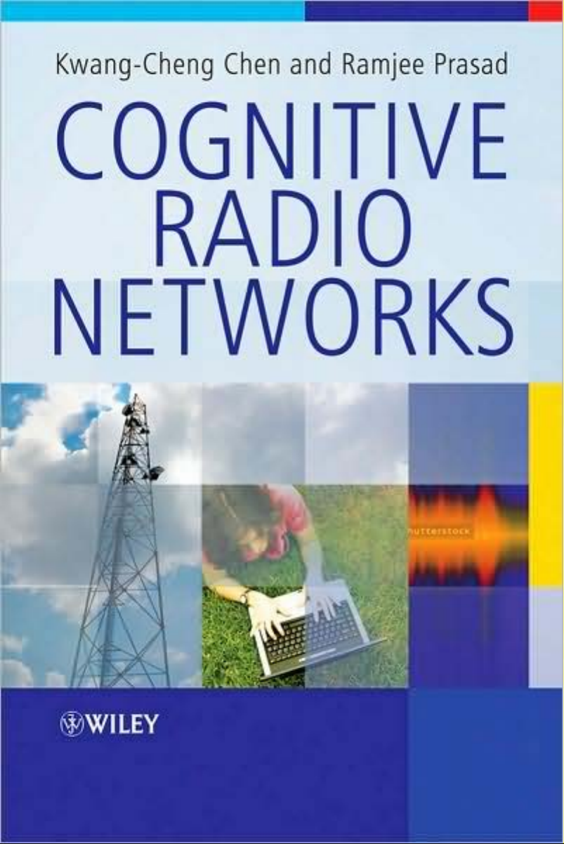
Figure 1.1 depicts the OSI seven-layer structure and its application to the general extension and
interconnection to other portion of networks. The four upper layers are mainly ‘logical’ rather than
‘physical’ in concept in network operation, whereas physical signalling is transmitted, received and
coordinated in the lower two layers: physical layer and data link layer. The physical layer of a wireless
network thus transmits bits and receives bits correctly in the wireless medium, while medium access
control (MAC) coordinates the packet transmission using the medium formed by a number of bits.
When we talk about wireless communications in this book, we sometimes refer it as a physical layer
and the likely MAC of wireless networks, although some people treat it with a larger scope. In this
chapter, we will focus on introducing physical layer transmission of wireless communication systems,
and several key technologies in the narrow-sense of wireless communications, namely orthogonal
frequency division multiplexing (OFDM) and multi-input-multi-output (MIMO) processing.
1.1 Wireless Communications Systems
To support multimedia traffic in state-of-the-art wireless mobile communications networks, digital
communication systemengineering has been used for the physical layer transmission. To allow a smooth
transitioninto laterchapters, we shall brieflyintroduce herethe fundamentals ofdigital communications,
Cognitive Radio Networks Kwang-Cheng Chen and Ramjee Prasad
©
2009 John Wiley & Sons Ltd. ISBN: 978-0-470-69689-7
Page 12
2 Cognitive Radio Networks
Application
Presentation
Session
Transport
Network
Data Link
Control
Physical
Virtual
Link for
Reliable
Packets
Virtual Bit
Pipe
Virtual Network Service
Virtual Session
Virtual End-to-End Link
(Message)
Virtual End-to-End Link(Packet)
Network
DLC DLC
PHYPHY
DLC DLC
Network
PHYPHY
SubnetSubnet
Application
Presentation
Session
Transport
Network
Data Link
Control
Physical
Figure 1.1 Seven-Layer OSI Network Architecture
assuming some knowledge of undergraduate-level communication systems and signalling. Interested
readers will find references towards more advanced study throughout the chapter.
Following analogue AM and FM radio, digital communication systems have been widely studied
for over half a century. Digital communications have advantages over their analogue counterparts due
to better system performance in links, and digital technology can also make media transmission more
reliable. In the past, most interest focused on conventional narrow-band transmission and it was
assumed that telephone line modems might lead the pace and approach a theoretical limit. Wireless
digital communications were led by major applications such as satellite communications and analogue
cellular. In the last two decades, wireless broadband communications such as code division multiple
access (CDMA) and a special form of narrowband transmission known as orthogonal frequency
division multiplexing (OFDM) were generally adopted in state-of-the-art communication systems for
high data rates and system capacity in complicated communication environments and harsh fading
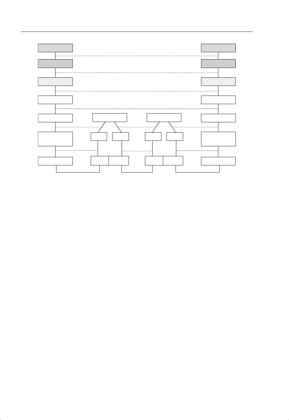
channels. A digital wireless communication system usually consists of the elements shown in
Figure 1.2, where they are depicted as a block diagram.
Information sources can be either digital, to generate 1s and 0s, or an analogue waveform source.
A source encoder then transforms the source into another stream of 1s and 0s with high entropy. Channel
coding, which proceeds completely differently from source coding, amends extra bits to protect
information from errors caused by the channel. To further randomise error for better information
protection, channel coding usually works with interleaving. In this case, bits are properly modulated,
which is usually a mapping of bits to the appropriate signal constellation. After proper filtering,
in typical radio systems, such baseband signalling is mixed through RF (radio frequency) and likely IF
(intermediate frequency) processing before transmission by antenna. The channel can inevitably
introduce a lot of undesirable effects, including embedded noise, (nonlinear) distortion, multi-path
fading and other impairments. The receiving antenna passes the waveform through RF/IF and an A/D
converter translates the waveform into digital samples in state-of-the-art digital wireless communication systems. Instead of reversing the operation at the transmitter, synchronisation must proceed so that
Page 13
Wireless Communications 3
Noise
Channel
Coding &
Interleaving
Channel
Decoding &
De-interleaving
Modulation
& Filtering
D/A
RF &
Antenna
Fading
Source
Decoding
Destination
Information
Source
Distortion
RF &
Antenna
A/D
Equalization Demodulation
Channel
Estimation
Source
Coding
Synchronization
Channel
Impairments
Figure 1.2 Block diagram of a typical digital wireless communication system
the right frequency, timing and phase can be recovered. To overcome various channel effects that
disrupt reliable communication, equalisation of these channel distortions is usually adopted. For further
reliable system design and possible pilot signalling, channel estimation to enhance receiver signal
processing can be adopted in many modern systems.
To summarise, the physical layer of wireless networks in wireless digital communications systems is
trying to deal with noise and channel impairments (nonlinear distortions by channel, fading, speed, etc.)
in the form of Inter Symbol Interference (ISI). State-of-the-art digital communication systems are
designed based on the implementation of these functions over hardware (such as integrated circuits) or
software running on top of digital signal processor(s) or micro-processor(s).
In the next section of this chapter, we focus on OFDM and its multiple access, Orthogonal Frequency
Division Multiple Access (OFDMA).
1.2 Orthogonal Frequency Division Multiplexing (OFDM)
In 1960, Chang [1] postulated the principle of transmitting messages simultaneously through a linear
band limited channel without Inter Channel Interference (ICI) and Inter Symbol Interference (ISI).
Shortly afterwards, Saltzberg [2] analysed the performance of such a system and concluded, ‘The
efficient parallel system needs to concentrate more on reducing crosstalk between the adjacent channels
rather than perfecting the individual channel itself because imperfection due to crosstalk tends to
dominate’. This was an important observation and was proven in later years in the case of baseband
digital signal processing.
The major contribution to the OFDM technique came to fruition when Weinstein and Ebert [3]
demonstrated the use of Discrete Fourier Transform (DFT) to perform baseband modulation and
demodulation. The use of DFT immensely increased the efficiency of modulation and demodulation
processing. The use of the guard space and raised-cosine filtering solve the problems of ISI to a great
extent. Although the system envisioned as such did not attain the perfect orthogonality between
subcarriers in a time dispersive channel, nonetheless it was still a major contribution to the evolution
of the OFDM system.
To resolve the challenge of orthogonality over the dispersive (fading) channel, Peled and Ruiz [4]
introduced the notion of the Cyclic Prefix (CP). They suggested filling the guard space with the cyclic
Page 14
4 Cognitive Radio Networks
extension of the OFDM symbol, which acts like performing the cyclic convolution by the channel
as long as the channel impulse response is shorter than the length of the CP, thus preserving the
orthogonality of subcarriers. Although addition of the CP causes a loss of data rate, this deficiency was
compensated for by the ease of receiver implementation.
1.2.1 OFDM Concepts
The fundamental principle of theOFDM system is to decomposethe high rate data stream(Bandwidth ¼
W)intoN lower rate data streams and then to transmit them simultaneously over a large number
of subcarriers. A sufficiently high value of N makes the individual bandwidth (W/N) of subcarriers
narrowerthan the coherencebandwidth(B
flat fading only and this can be compensated for using a trivial frequency domain single tap equaliser.
The choice of individual subcarrier is such that they are orthogonal to each other, which allows for the
overlapping of subcarriers becausethe orthogonality ensures the separationof subcarriers at the receiver
end. This approach results in a better spectral efficiency compared to FDMA systems, where no spectral
overlap of carriers is allowed.
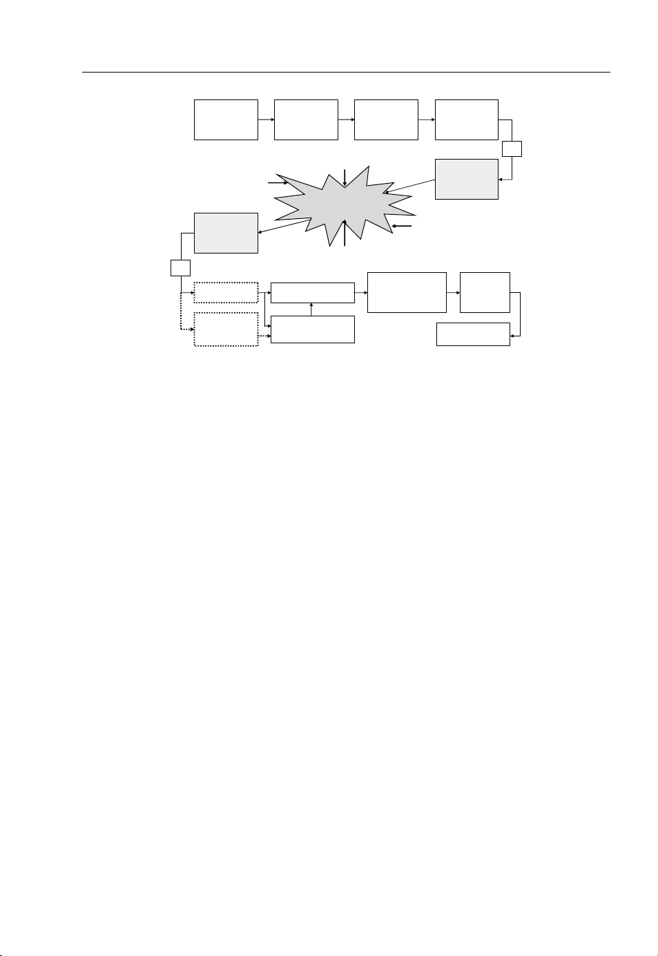
The spectral efficiency of an OFDM system is shown in Figure 1.3, which illustrates the difference
between the conventional non-overlapping multicarrier technique (such as FDMA) and the overlapping
multicarrier modulation technique (such as DMT, OFDM, etc.). As shown in Figure 1.3 (for illustration
purposes only; a realistic multicarrier technique is shown in Figure 1.5), use of the overlapping
multicarrier modulation technique can achieve superior bandwidth utilisation. Realising the benefits of
the overlapping multicarrier technique, however, requires reduction of crosstalk between subcarriers,
which translates into preserving orthogonality among the modulated subcarriers.
) of the channel. The individual subcarriers as such experience
c
Figure 1.3 Orthogonal multicarrier versus conventional multicarrier
The ‘orthogonal’ dictates a precise mathematical relationship between frequencies of subcarriers
in the OFDM based system. In a normal frequency division multiplex system, many carriers are spaced
Page 15
Wireless Communications 5
apart in such a way that the signals can be received using conventional filters and demodulators. In such
receivers, guard bands are introduced between the different carriers in the frequency domain, which
results in a waste of the spectrum efficiency. However, it is possible to arrange the carriers in an OFDM
system such that the sidebands of the individual subcarriers overlap and the signals are still received
without adjacent carrier interference. The OFDM receiver can therefore be constructed as a bank of
demodulators, translating each subcarrier down to DC and then integrating over a symbol period to
recover the transmitted data. If all subcarriers down-convert to frequencies that, in the time domain,
have a whole number of cycles in a symbol period T, then the integration process results in zero ICI.
These subcarriers can be made linearly independent (i.e., orthogonal) if the carrier spacing is a multiple
of 1/T, which will be proven later to be the case for OFDM based systems.
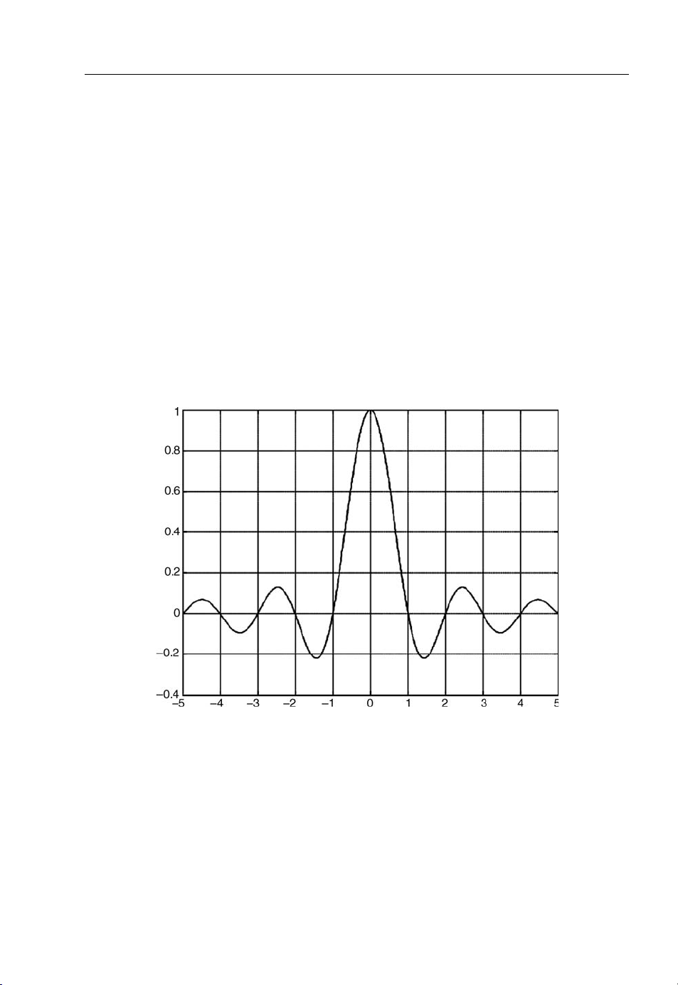
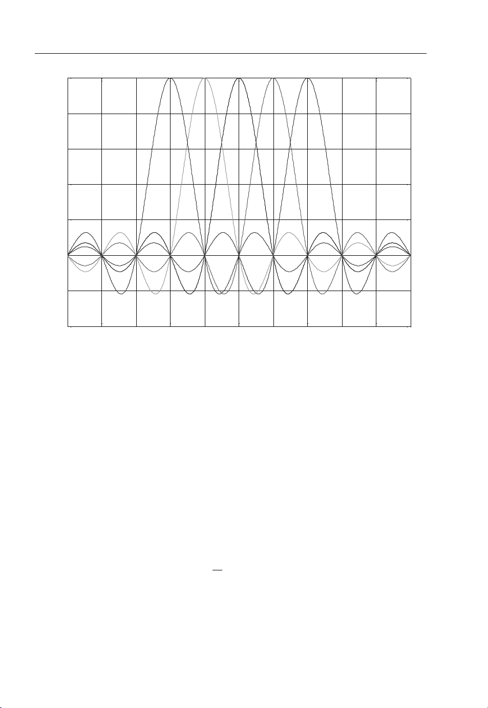
Figure 1.4 shows the spectrum of an individual data subcarrier and Figure 1.5 depicts the spectrum
of an OFDM symbol. The OFDM signal multiplexes in the individual spectra with a frequency spacing
equal to the transmission bandwidth of each subcarrier as shown in Figure 1.4. Figure 1.5 shows that at
the centre frequency of each subcarrier there is no crosstalk from other channels. Therefore, if a receiver
performs correlation with the centre frequency of each subcarrier, it can recover the transmitted data
without any crosstalk. In addition, using the DFT based multicarrier technique, frequency-division
multiplexing is achieved by baseband processing rather than the costlier bandpass processing.
Figure 1.4 Spectra of OFDM individual subcarrier
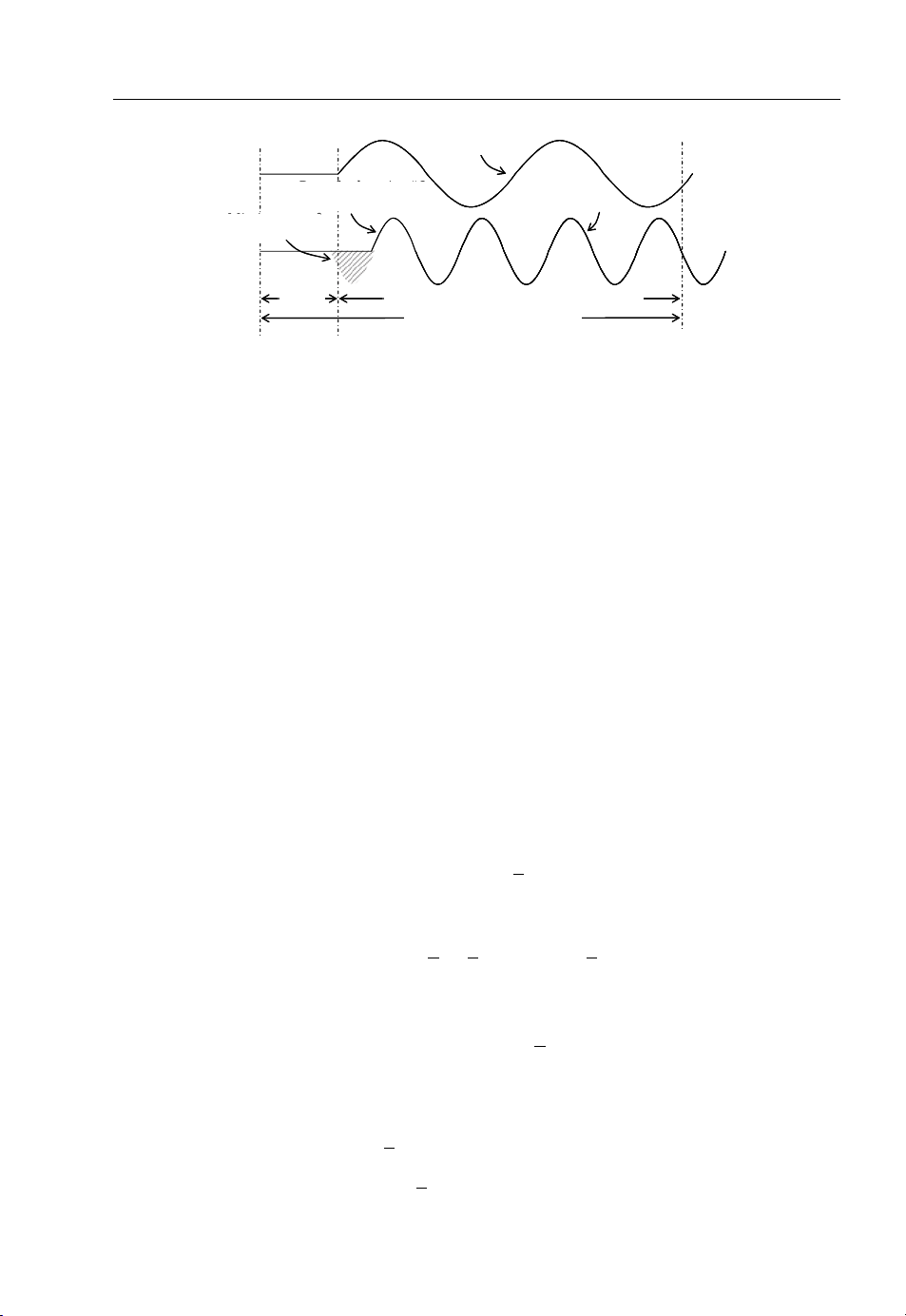
The orthogonality of subcarriers is maintained even in the time-dispersive channel by adding the CP.
The CP is the last part of an OFDM symbol, which is prefixed at the start of the transmitted OFDM
symbol, which aids in mitigating the ICI related degradation. Simplified transmitter and receiver block
diagrams of the OFDM system are shown in Figures 1.6 (a) and (b) respectively.
1.2.2 Mathematical Model of OFDM System
OFDM based communication systems transmit multiple data symbols simultaneously using orthogonal
subcarriers as shown in Figure 1.7. A guard interval is added to mitigate the ISI, which is not shown
Page 16
6 Cognitive Radio Networks
1
0.8
0.6
0.4
0.2
0
–0.2
–0.4
–5 –4 –3 –2 –1 0 1 2 3 4 5
Figure 1.5 Spectra of OFDM symbol
in the figure for simplicity. The data symbols (d
then modulated with complex orthonormal (exponential in this book) waveform ff
) are first assembled into a group of block size N and
n,k
k
ðtÞg
N
k¼0
as shown
in Equation (1.1). After modulation they are transmitted simultaneously as transmitter data stream.
The modulator as shown in Figure 1.7 can be easily implemented using an Inverse Fast Frequency
Transform (IFFT) block described by Equation (1.1):
"#
¥
N 1
X
xðtÞ¼
X
n¼¥
k¼0
d
fkðt nTdÞ
n;k
ð1:1Þ
where
j2pfkt
f
ðtÞ¼
k
e
t«½0; Td
0 otherwise
and
¼ foþ
k
; k ¼ 0 ...N 1
T
d
f
k
We use the following notation:
&
d
: symbol transmitted during nth timing interval using kth subcarrier;
n,k
&
Td: symbol duration;
&
N: number of OFDM subcarriers;
&
fk: kth subcarrier frequency, with f0being the lowest.
Page 17

Wireless Communications 7
Figure 1.6 (a) Transmitter block diagram and (b) receiver block diagram
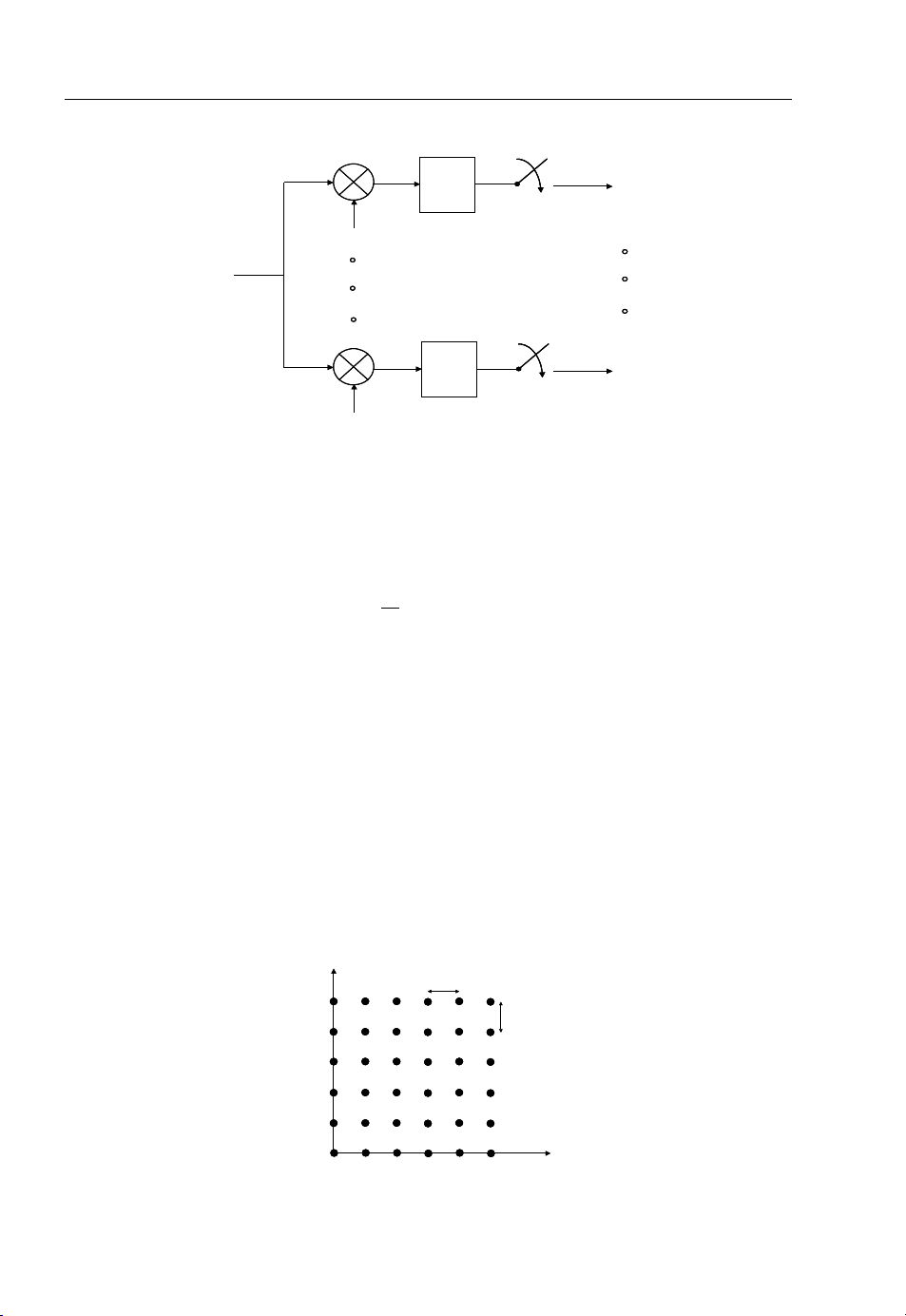
The simplified block diagram of an OFDM demodulator is shown in Figure 1.8. The demodulation
process is based on the orthogonality of subcarriers {f
ð
*
fkðtÞf
R
d
n,0
d
n,N–1
ðtÞdt ¼ Tddðk lÞ¼
l
tjw
0
e
tjw
N−1
e
(t)}, namely:
k
T
d
0 otherwise
Σ
k ¼ l
x(t)
Figure 1.7 OFDM modulator
Page 18
x
8 Cognitive Radio Networks
T
d
d
)(
•
∫
T
T
t
−jw
0
e
d
n,0
(t)
T
d
d
)(
•
∫
T
T
t
−jNw
0
e
d
n,N–1
Figure 1.8 OFDM demodulator
Therefore, a demodulator can be implemented digitally by exploiting the orthogonality relationship
of subcarriers yielding a simple Inverse Fast Frequency Transform (IFFT)/Fast Frequency Transform
(FFT) modulation/demodulation of the OFDM signal:
ðn þ 1ÞT
d
ð
1
¼
d
n;k
T
d
nT
xðtÞ*f
d
*
ðtÞdt ð1:2Þ
k
Equation (1.2) can be implemented using the FFT block as shown in Figure 1.8.
The specified OFDM model can also be described as a 2-D lattice representation in time and
frequency plane and this property can be exploited to compensate for channel related impairments
issues. Looking into the modulator implementation of Figure 1.7, a model can be devised to represent
the OFDM transmitted signal as shown in Equation (1.3). In addition, this characteristic may also be
exploited in pulse shaping of the transmitted signal to combat ISI and multipath delay spread. This
interpretation is detailed in Figure 1.8.
X
dkf
xðtÞ¼
k;l
ðtÞð1:3Þ
k;l
The operand fk,l(t), represents the time and frequency displaced replica of basis function f(t)by
and kn0in 2-D time and frequency lattice respectively and as shown in Figure 1.9. Mathematically it
lt
0
τ
0
ν
0
Frequency
Time
Figure 1.9 2-D lattice in time-frequency domain
Page 19

Wireless Communications 9
can be shown that operand f
Usually the basis function f(t) is chosen as a rectangular pulse of amplitude 1=
t
and the frequency separation are set at y0¼1/t0.Each transmitted signal in the lattice structure
0
(t) is related to the basis function in Equation (1.4) as follows:
k,l
f
ðtÞ¼fðt lt0Þe
k;l
j2pky0t
p
ffiffiffiffiffi
and duration
t
0
ð1:4Þ
experiences the same flat fading during reception, which simplifies channel estimation and the
equalisation process. The channel attenuations are estimated by correlating the received symbols
with a priori known symbols at the lattice points. This technique is frequently used in OFDM based
communication systems to provide the pilot assisted channel estimation.
1.2.3 OFDM Design Issues
Communication systems based on OFDM have advantages in spectral efficiency but at the price of
being sensitive to environment impairments. To build upon the inherent spectral efficiency and simpler
transceiver design factors, these impairment issues must be dealt with to garner potential benefits.
In communication systems, a receiver needs to synchronise with a transmitter in frequency, phase and
time (or frame/slot/packet boundary) to reproduce the transmitted signal faithfully. This is not a trivial
task particularly in a mobile environment, where operating conditions and surroundings vary so
frequently. For example, when a mobile is turned on, it may not have any knowledge of its surroundings
and it must take few steps (based upon agreed protocol/standards) to establish communication with the
base station/access point. This basic process in communication jargon is known as synchronisation and
acquisition. The tasks of synchronisation and acquisition are complex issues anyway, but impairments
make things even harder. Impairment issues are discussed in detail in the following sections.
1.2.3.1 Frequency Offset
Frequency offset in an OFDM system is introduced from two sources: mismatch between transmit and
receive sampling clocks and misalignment between the reference frequency of transmit and receive
stations. Both impairments and their effects on the performance are analysed.
The sampling epoch of the received signal is determined by the receiver A/D sampling clock, which
seldom resumes the exact period matching the transmit sampling clock causing the receiver sampling
instants slowly to drift relative to the transmitter. Many authors have analysed the effect of sampling
clock drift on system performance. The sampling clock error manifests in two ways: first, a slow
variation in the sampling time instant causes rotation of subcarriers and subsequent loss of the SNR
due to ICI, and second, it causes the loss of orthogonality among subcarriers due to energy spread
among adjacent subcarriers. Let us define the normalised sampling error as
T0T
¼
t
D
T
where T and T
DFT, on the received subcarriers R
where l is the OFDM symbol index, k is the subcarrier index, T
the useful duration of thesymbol duration respectively,W
term N
t
approximated by P
0
are transmit and receive sampling periods respectively. Then, the overall effect, after
can be shown as:
l,k
T
s
j2pktDl
T
R
¼ e
l;k
is the additional interference due to the sampling frequency offset.The power of the last term is
D
2
p
ðktDÞ2.
t
D
3
u
X
sin cðpktDÞH
l;k
l;kþWl;kþNt
and Tuare the duration of the total and
s
is additivewhite Gaussian noise and the last
l,k
ðl; kÞ
D
Page 20
g
10 Cognitive Radio Networks
Hence, the degradation grows as the square of the product of offset tDand the subcarrier index k. This
means that the outermost subcarriers are most severely affected. The degradation can also be expressed
as SNR loss in dB by following expression:
2
p
E
s
10 log101 þ
D
n
3
N
ðktDÞ
0
2
In OFDM systems with a small number of subcarriers and quite small sampling error t
1, the degradation caused by the sampling frequency error can be ignored. The most significant
kt
D
issue is the different value of rotation experienced by the different subcarriers based on the subcarrier
index k and symbol index l; this is evident from the term {e
T
s
j2pktDl
T
u
}. Hence, the rotation angle is the
largest for the outermost subcarrier and increases as a function of symbol index l. The term t
such that
D
D
controlled by the timing loop and usually is very small, but as l increases the rotation eventually
becomes so large that the correct demodulation is no longer possible and this necessitates the tracking
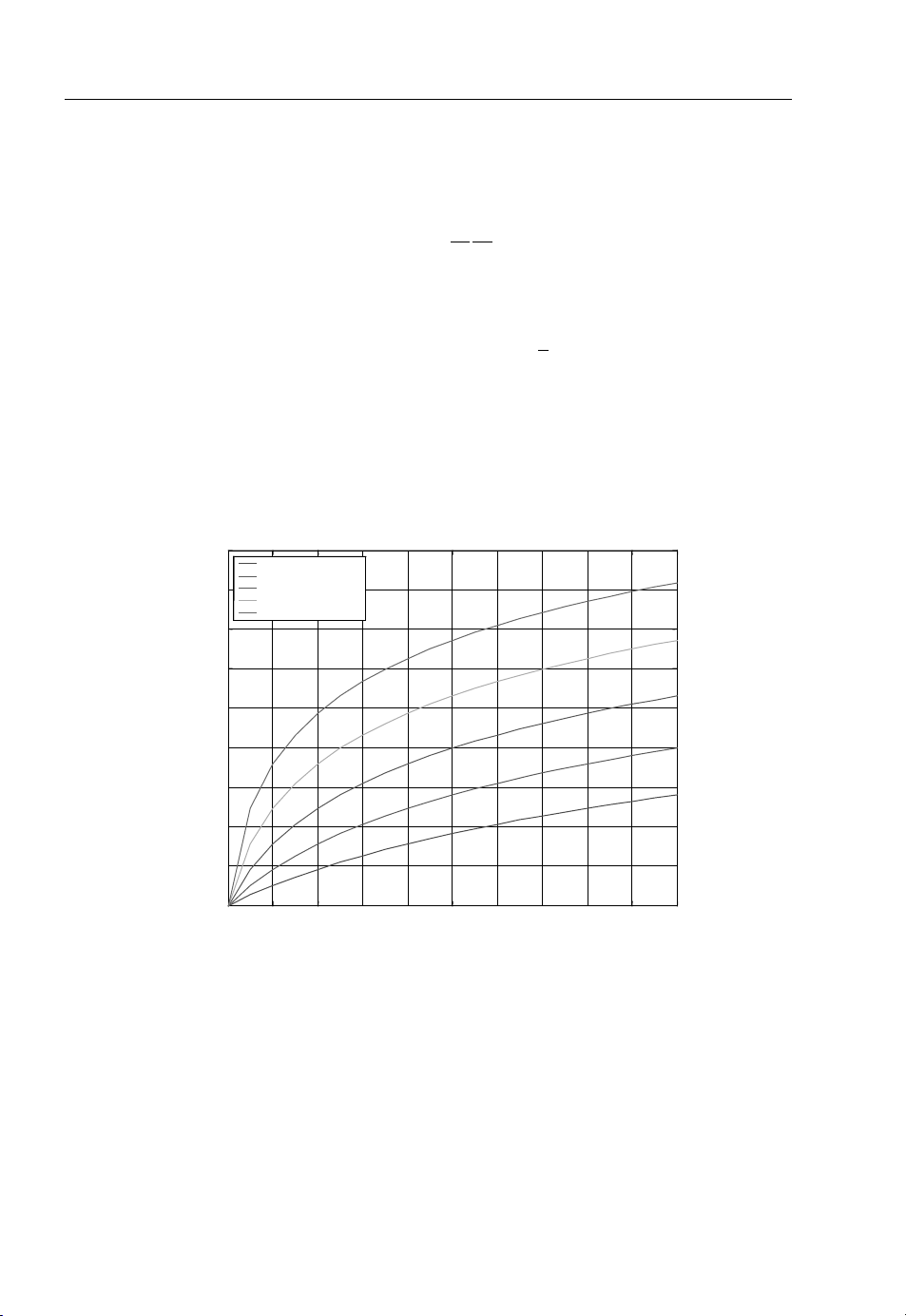
of the sampling frequency in the OFDM receiver. The effect of sampling offset on the SNR degradation
is shown in Figure 1.10.
SNR Degradation Due to Sampling Offset
18
Num Subcarriers = 4
Num Subcarriers = 8
Num Subcarriers = 16
16
Num Subcarriers = 32
Num Subcarriers = 64
14
12
10
Loss
(dB)
8
6
4
is
2
0
0 0.02 0.04 0.06 0.08 0.1 0.12 0.14 0.16 0.18 0.2
Normalized Samplin
Offset
Figure 1.10 SNR degradation due to sampling mismatch
1.2.3.2 Carrier Frequency Offset
The OFDM systems are much more sensitive to frequency error compared to the single carrier
frequency systems. The frequency offset is produced at the receiver because of local oscillator
instability and operating condition variability at transmitter and receiver; Doppler shifts caused by
the relative motion between the transmitter and receiver; or the phase noise introduced by other channel
impairments. The degradation results from the reduction in the signal amplitude of the desired
subcarrier and ICI caused by the neighbouring subcarriers. The amplitude loss occurs because
the desired subcarrier is no longer sampled at the peak of the equivalent sinc-function of the DFT.
Page 21

Wireless Communications 11
Adjacent subcarriers cause interference because they are not sampled at their zero crossings. The
overall effect of carrier frequency offset effect on SNR is analysed by Pollet et al [6] and for relatively
small frequency error, the degradation in dB is approximated by
SNR
ðdBÞ
loss
10
3ln10
ðpTf
E
s
2
Þ
D
N
0
where fDis the frequency offset and is a function of the subcarrier spacing and T is the sampling period.
The performance of the system depends on modulation type. Naturally, the modulation scheme with
large constellation points is more susceptible to the frequency offset than a small constellation modulation scheme, because the SNR requirements for the higher constellation modulation scheme are much
higher for the same BER performance.
It is assumed that two subcarriers of an OFDM system can be represented using the orthogonal
frequency tones at the output of the A/D converter at baseband as
f
k
ðtÞ¼e
j2pfkt=T
and f
k þ m
ðtÞ¼e
j2pðk þmÞt=T
where T is the sampling period. Let us also assume that due to the frequency drift the receive station has
a frequency offset of d from kth tone to (k þ m)th tone, i.e.,
f
d
k þ m
ðtÞ¼e
j2pðk þm þdÞt=T
Due to this frequency offset there is an interference between kth and (k þ m)th channels given by
T
I
ðdÞ¼
m
ð
jk2pt=Tejðk þ m þdÞ2pt=T
e
0
jI
ðdÞj ¼
m
dt ¼
TjsinðpdÞj
pjm þdj
j2pd
Tð1 e
j2pðm þdÞ
Þ
The aggregate loss (power) due to this interference from all N subcarriers can be approximated as
following:
N 1
X
m
2
I
ðdÞðTdÞ
m
X
1
2
m¼1
m
ðTdÞ
2
2
23
14
for N 1
1.2.3.3 Timing Offset
The symbol timing is very important to the receiver for correct demodulation and decoding of the
incoming data sequence. The timing synchronisation is possible with the introduction of the training
sequences in addition to the data symbols in the OFDM systems. The receiver may still not be able to
recover the complete timing reference of the transmitted symbol because of the channel impairments
causing the timing offset between the transmitter and the receiver. A time offset gives rise to the phase
rotation of the subcarriers. The effect of the timing offset is negated with the use of a CP. If the channel
response due to timing offset is limited within the length of the CP the orthogonality across the
subcarriers are maintained. The timing offset can be represented by a phase shift introduced by the
channel and can be estimated from the computation of the channel impulse response. When the receiver
is not time synchronised to the incoming data stream, the SNR of the received symbol is degraded.
Page 22

12 Cognitive Radio Networks
The degradation can be quantised in terms of the output SNR with respect to an optimal sampling time,
, as shown below:
T
optimal
LðtÞ
z ¼
Lð0Þ
where T
T
optimal
is the autocorrelation function and t is the delay between the optimal sampling instant
optimal
and the received symbol time. The parameter t is treated as a random variable since it is
estimated in the presence of noise and is usually referred as the timing jitter. The two special cases of
interest, baseband time-limited signals and band-limited signals with the normalised autocorrelation
functions, are shown below in mathematical forms:
LðtÞ¼ 1
LðtÞ¼
1NsinðpNWtÞ
tjj
T
symbol
sinðpWtÞ
where W is the bandwidth of the band-limited signal. The single carrier system is best described as the
band-limited signal whereas the OFDM (multicarrier) system is best described as the time-limited
signal. For single carrier systems, the timing jitter manifests as a noisy phase reference of the bandpass
signal. In the case of OFDM systems, pilot tones are transmitted along with the data-bearing carrier to
estimate residual phase errors.
Paez-Borrallo [7]has analysed the loss of orthogonality due to time shift and the result of this analysis
is shown here to quantise its effect on ICI and the resulting loss in orthogonality. Let us assume the
timing offset between the two consecutive symbols is denoted by t, then the received stream at the
receiver can be expressed as follows:
ð
T =2 þt
¼ c
X
i
0
T =2
fkðtÞf
*
ðt tÞdt þc
l
ð
1
T=2
T =2 þt
fkðtÞf
*
ðt tÞdt
l
where
j2pfkt=T
ðtÞ¼e
f
k
Substitute m ¼k l and then the magnitude of the received symbol can be represented as
jX
8
>
sin mp
>
<
2T
j¼
i
>
>
:
0; c0¼ c
mp
t
T
; c
„ c
0
1
1
This can be further simplified for simple analysis if t T:
jXij
T
mp
t
T
¼ 2
T
t
2mp
This is independent of m, for t T.
We can compute the average interfering power as
"#
2
jXij
E
¼ 4
2
T
2
t
1
þ0
T
2
1
¼ 2
2
2
t
T
Page 23

Wireless Communications 13
The ICI loss in dB is computed as follows:
2
ICI
dB
¼ 10 log102
t
T
1.2.3.4 Carrier Phase Noise
The carrier phase impairment is induced due to the imperfection in the transmitter and the receiver
oscillators. The phase rotation could either be the result of the timing error or the carrier phase offset for
a frequency selective channel. The analysis of the system performance due to carrier phase noise
has been performed by Pollet et al. [8] The carrier phase noise was modelled as the Wiener process u (t)
with E {q (t)} ¼0 and E [{q (t
þ t) q(t0)}2] ¼4pb|t|, where b (in Hz) denotes the single sided
0
line width of the Lorentzian power spectral density of the free running carrier generator. Degradation
in the SNR, i.e., the increase in the SNR needed to compensate for the error, can be approximated by
DðdBÞ
11
6ln10
4pN
b
E
s
W
N
0
where W is the bandwidth and Es/N0is the SNR of the symbol. Note that the degradation increases with
the increase in the number of subcarriers.
1.2.3.5 Multipath Issues
In mobile wireless communications, a receiver collects transmitted signals through various paths, some
arriving directly and some from neighbouring objects because of reflection, and some even arriving
because of diffraction from the nearby obstacles. These arriving paths arriving at the receiver may
interfere with each other and cause distortion to the information-bearing signal. The impairments
caused by multipath effects include delay spread, loss of signal strength and widening of frequency
spectrum. The random nature of the time variation of the channel may be modelled as a narrowband
statistical process. For a large number of signal reflections impinging on the receive antenna, the
distribution of the arriving signal can be modelled as complex-valued Gaussian Random Processes
based on central limit theory. The envelope of the received signal can be decomposed into fast varying
fluctuations superimposed onto slow varying ones. When the average amplitude of envelope suffers
a drastic degradation from the interfering phase from the individual path, the signal is regarded as
fading. Multipath is a term used to describe the reception of multiple copies of the information-bearing
signal by the receive antenna. Such a channel can be described statistically and can be characterised
by the channel correlation function. The baseband-transmitted signal can be accurately modelled as a
narrowband process as follows:
sðtÞ¼xðtÞe
2pfct
Assuming the multipath propagation as Gaussian scatterers, the channel can be characterised by time
varying propagation delays, loss factors and Doppler shifts. The time-varying impulse response of the
channel is given by
X
where c(t
; tÞ¼
cðt
n
, t) is the response of the channel at time t due to an impulse applied at time t tn(t); an(t)
n
anðtn; tÞe
n
is the attenuation factor for the signal received on the nth path; t
nth path; and f
is the Doppler shift for the signal received on the nth path.
D
n
j2pf
tnðtÞ
D
n
d½t tnðtÞ
(t) is the propagation delay for the
n
Page 24

14 Cognitive Radio Networks
The Doppler shift is introduced because of the relative motion between the transmitter and the
receiver and can be expressed as
v cosðunÞ
¼
f
D
n
l
where v is the relative velocity between transmitter and receiver, l is the wavelength of the carrier and
q
is the phase angle between the transmitter and the receiver.
n
The output of the transmitted signal propagating through channel is given as
; tÞ*sðtÞ
n
ÞtnðtÞ
D
n
xðt tnðtÞÞe
j2pfct
zðtÞ¼
X
an½tnðtÞe
n
zðtÞ¼cðt
j2pðfcþf
where
ðtÞÞ*xðtÞ¼xðt tnðtÞÞ
dðt t
n
dðt t
ðtÞÞ*e
n
bn¼ antnðtÞ½e
j2pfct
j2pfcðt tnðtÞÞ
¼ e
j2pðfcþf
D
ÞtnðtÞ
n
Alternately z(t) can be written as
zðtÞ¼
X
bnxðt tnðtÞÞe
n
j2pfct
where bnis the Gaussian random process. The envelope of the channel response function c(tn, t) has
a Rayleigh distribution function because the channel response is the ensemble of the Gaussian random
process. The density function of a Rayleigh faded channel is given by
2
z
z
2
f
ðzÞ¼
z
2s
e
2
s
A channel without a direct line of sight (LOS) path (i.e., only scattered paths) is typically termed a
Rayleigh fading channel. A channel with a direct LOS path to the receiver is generally characterised
by a Rician density function and is given by
ðzÞ¼
f
z
z
s
I
0
2
zh
s
e
2
2
z2þh
2
2s
where I
is the modified Bessel function of the zeroth order and h and s2are the mean and variance
0
of the direct LOS paths respectively. Proakis [9] has shown the autocorrelation function of c(t, t)as
follows:
ðt; DtÞ¼Efcðt; tÞc*ðt; t þDtÞg
L
c
In addition, it can be measured by transmitting very narrow pulses and cross correlating the received
signal with a conjugate delayed version of itself. The average power of the channel can be found by
setting Dt ¼ 0, i.e., L
intensity profile. The range of values of t over which L
(t, Dt) ¼ Lc(t). The quantity is known as the power delay profile or multipath
c
(t) is essentially nonzero is called the multipath
c
Page 25

Wireless Communications 15
delay spread of the channel, denoted by tm. The reciprocal of the multipath delay spread is a measure of
the coherence bandwidth of the channel, i.e.,
1
B
m
t
m
The coherence bandwidth of a channel plays a prominent role in communication systems. If the
desired signal bandwidth of a communication system is small compared to the coherence bandwidth
of the channel, the system experiences flat fading (or frequency non-selective fading) and this eases
signal processing requirements of the receiver system because the flat fading can be overcome by
adding the extra margin in the system link budget. Conversely, if the desired signal bandwidth is large
compared to the coherence bandwidth of the channel, the system experiences frequency selective
fading and impairs the ability of the receiver to make the correct decision about the desired signal.
The channels, whose statistics remain constant for more than one symbol interval, are considered a slow
fading channel compared to the channels whose statistics change rapidly during a symbol interval.
In general, broadband wireless channels are usually characterised as slow frequency selective fading.
1.2.3.6 Inter Symbol Interference (ISI) Issues
The output of the modulator as shown in Equation (1.1) is shown here for reference
"#
¥
N 1
X
n¼¥
X
k¼0
d
fkðt nTdÞ
n;k
xðtÞ¼
Equation (1.1) can be re-written in the discrete form for the nth OFDM symbol as follows:
N 1
X
where f
For the n
j2pfkt/T
(t) ¼e
k
th
block of channel symbols, dnP, d
.
x
n
ðkÞ¼
k¼0
d
fkðt nTdÞ
n;k
...d
nP þ 1
nP þ P 1
, the ithsubcarrier signal can be
expressed as follows:
N 1
ðkÞ¼
X
d
k¼0
where l
i
x
n
the index of time complex exponential of length N, i.e., 0 liN -1.
i
These are summed to form the n
nP þ i;k
2p
j
lik
N
e
For i ¼ 0; 1; 2 ...P 1; P ¼ number of subcarriers
th
OFDM symbol given as
ðkÞ
x
n
P 1
X
i¼0
x
0
ðkÞ¼
n
P 1
X
i¼0
d
nP þ i
2p
j
lik
N
e
ð1:5Þ
The transmitted signal at the output of the digital-to-analogue converter can be represented as
follows:
"#
L 1
X
X
sðtÞ
n
xnðkÞdðt ðnL þkÞTdÞ
k¼0
where, L is the length of data symbol larger than N (number of subchannels). Since the sequence length
L is longer than N, only a subset of the OFDM received symbols are needed at thereceiver to demodulate
Page 26

16 Cognitive Radio Networks
the subcarriers. The additional Q ¼L N symbols are not needed and we will see later that it could be
used as a guard interval to add the CP to mitigate the ICI problem in OFDM systems. In multipath and
additive noise environments, the received OFDM signal is given by
ðkÞ¼
r
n
L 1
X
xnðiÞhðk iÞþ
i¼0
L 1
X
i¼0
x
ðiÞhðk þL iÞþvnðkÞð1:6Þ
n 1
The first term represents the desired information-bearing signal in a multipath environment, whereas
the second part represents the interference from the preceding symbols. The length of the multipath
channel, L
, is assumed much smaller than the length of the OFDM symbol L. This assumption plus the
h
assumption about the causality of the channel implies that the ISI is only from the preceding symbol.
If we assume that the multipath channel is as long as the guard interval, i.e., L
Q, then the received
h
signal can be divided into two time intervals. The first time intervalcontains the desired symbol plus the
ISI from the preceding symbol. The second interval contains only the desired information-bearing
symbol. Mathematically it can be written as follows:
8
ðkÞ¼
r
n
L 1
X
>
>
>
xnðiÞhðk iÞþ
>
<
i¼0
L 1
>
X
>
>
>
xnðiÞhðk iÞþvnðkÞ Q k L 1
:
i¼0
L 1
X
i¼0
x
ðiÞhðk þL iÞþvnðkÞ 0 k Q 1
n 1
ð1:7Þ
We are ready to explore the performance degradation due to ISI. ISI is the effect of the time dispersion
of the information-bearing pulses, which causes symbols to spread out so that they disperse energy
into the adjacent symbol slots. The Nyquist criterion paves the way to achieve ISI-free transmission
with observation at the Nyquist rate samples in a band limited environment, to result in zero-forcing
equalisation. The complexity of the equaliser depends on the severity of the channel distortion.
Degradation occurs due to the receiver’s inability to equalise the channel perfectly, and from the noise
enhancement of the modified receiver structure in the process. The effect of the smearing of energy into
the neighbouring symbol slots is represented by the second term in Equation (1.7). The effect of the ISI
can be viewed in time and frequency domain.
One of the most important properties of the OFDM system is its robustness against multipath delay
spread, ISI mitigation. This is achieved by using spreading bits into a number of parallel subcarriers to
result in a long symbol period, which minimises the inter-symbol interference. The level of robustness
against the multipath delay spread can be increased even further by addition of theguard period between
transmitted symbols. The guard period allows enough time for multipath signals from the previous
symbol to die away before the information from the current symbol is gathered. The most effective use
of guard period is the cyclic extension of the symbol. The end part of the symbol is appended at the start
of the symbol inside the guard period to effectively maintain the orthogonality among subcarriers.
Using the cyclically extended symbol, the samples required for performing the FFT (to decode the
symbol) can be obtained anywhere over the length of the symbol. This provides multipath immunity as
well as symbol time synchronisation tolerance.
As long as the multipath delays stay within the guard period duration, there is strictly no limitation
regarding the signal level of the multipath; they may even exceed the signal level of the shorter path.
The signal energy from all paths just adds at the input of the receiver, and since the FFT is energy
conservative, the total available power from all multipaths feeds the decoder. When the delay spread is
larger than the guard interval, it causes the ISI. However, if the delayed path energies are sufficiently
small then they may not cause any significant problems. This is true most of the time, because path
delays longer than the guard period would have been reflected of very distant objects and thus have been
diminished quite a lot before impinging on the receive antenna.
Page 27
Wireless Communications 17
Subcarrier # 1
Subcarrier # 1
Part of subcarrier # 2
Part of subcarrier # 2
causing ICI
Missing part of
Missing part of
Sinusoid
Sinusoid
Guard
Guard
Time
Time
causing ICI
FFT Integration Time = 1/Carrier Spacing
FFT Integration Time = 1/Carrier Spacing
OFDM Symbol Time
OFDM Symbol Time
Subcarrier #2
Subcarrier #2
Figure 1.11 Effect of multipath on the ICI
The disaster of OFDM systems is ICI, which is introduced due to the loss of the orthogonality of
subcarriers. The loss of orthogonality may be due to the frequency offset, the phase mismatch or
excessive multipath dispersion. The effect of this is illustrated in Figure 1.11, where subcarrier-1 is
aligned to the symbol integration boundary, whereas subcarrier-2 is delayed. In this case, the receiver
will encounter interference because the number of cycles for the FFT duration is not the exact multiple
of the cycles of subcarrier-2. Fortunately, ICI can be mitigated with intelligent exploitation of the guard
period, which is required to combat the ISI. The frequency offset between the transmitter and the
receiver generates residual frequency error in the received signal. The effect of the frequency offset can
be analysed analytically by expanding upon Equation (1.7) as follows:
8
ðkÞ¼
r
n
L 1
X
>
>
>
xnðiÞhðk iÞþ
>
<
i¼0
L 1
X
>
>
>
xnðiÞhðk iÞþvnðkÞ Q k L 1
>
:
i¼0
L 1
X
i¼0
x
ðiÞhðk þL iÞþvnðkÞ 0 k Q 1
n 1
ð1:8Þ
At the receiverthe guard period isdiscardedand the remainingsignal is defined for k ¼0, 1...N -1as
0
r
ðkÞrnðk þQÞð1:9Þ
n
Substitute Equation (1.5) into Equation (1.9), which after simplification yields the following:
0
r
ðkÞ¼
n
X
a
hðaÞ
X
2p
j
liðk þ Q a Þ
nP þ i
N
e
þvnðkÞ
d
i
or,
0
ðkÞ¼
r
n
X
2p
j
likej
N
d
e
nP þ i
i
X
2p
liQ
N
hðaÞe
a
2p
j
lia
N
þvnðkÞð1:10Þ
Equation (1.10) can be written in a simplified form as
X
0
ðkÞ¼
r
n
0
The (
) is dropped from the equation without the loss of generality
d
fiHðliÞe
nP þ i
i
where
2p
j
liQ
N
f
Hðl
Þ¼
i
X
a
i
¼ e
hðaÞe
Constant phase multiplier
2p
j
lia
N
Fourier Transform of the hðnÞ
2p
j
lik
N
þvnðkÞð1:11Þ
Page 28
18 Cognitive Radio Networks
The received signal with frequency-offset Df can be plugged into Equation (1.11) to yield the
following:
off
ðkÞrnðkÞe
r
n
j2pDfk
X
¼
d
fiHðliÞe
nP þ i
i
2p
j
kðliþDfN Þ
N
þVnðkÞð1:12Þ
It can be shown from Equation (1.12) that the frequency offset induces ICI as well the loss of
orthogonality between subcarriers, which degrades performance by this ICI. In other words, the symbol
estimate becomes
^
d
nP þ i
2
6
¼ GifHðliÞd
4
nP þ iIDf
ð0Þgþ
8
>
<
>
:
P 1
X
i¼0
i „ m
HðlmÞd
nP þ iIDfðlmli
ÞgþVnðliÞ
3
7
5
ð1:13Þ
where the ICI term is
I
Dfðlmli
Þ¼e
ð1:14Þ
2p
j
kðlmliþDfN Þ
N
Starting from Equation (1.14) it can be shownthat the SNR degradation due to small frequency offset
is approximately
where E
SNR
ðdBÞ
loss
is the SNR in the absence of the frequency offset.
s/N0
10
3ln10
ðpDfNT
E
s
2
Þ
s
N
0
ð1:15Þ
Please recall that ISI is eliminated by introducing a guard period for each OFDM symbol. The guard
period is chosen larger than the expected delay spread such that multipath components from one symbol
do not interfere with adjacent symbols. This guard period could be no signal at all but the problem of ICI
would still exist. To eliminate ICI, the OFDM symbol is cyclically extended in the guard period as
shown in Figure 1.12, bytwo intuitive approaches using cyclic prefix and/or cyclic suffix to facilitate the
guard band. This ensures that the delayed replicas of the OFDM symbols due to multipath will always
have the integer number of cycles within the FFT interval, as long as delay is smaller than the guard
period. As a result, multipath signals with delays smaller than the guard period do not cause ICI.
Cyclic Suffix
tTs0
Tg
Original OFDM
tTs0
Cyclic Prefix
Tg
Figure 1.12 Cyclic prefix in the guard period
tTs0
Page 29

Wireless Communications 19
Mathematically it can be shown that the cyclic extension of the OFDM symbol in the guard period
makes the OFDM symbol appear periodic at the receiver end even though there might be a delay
because of the multipath environment. In OFDM system the N complex-valued frequency domain
symbols X(n),0 < n < N -1, modulate N orthogonal carriersusing the IDFTproducing domain signal
as follows:
N 1
xðkÞ¼
X
XðnÞe
n¼0
þj2pk
n
N
¼ IDFT XðnÞ
fg
ð1:16Þ
The basic functions of the IDFT are orthogonal. By adding a cyclic prefix, the transmitted signal
appears periodic:
sðkÞ¼
xðk þNÞ 0 k < Q
xðkÞ Q k < L
where Q is the length of the guard period. The received signal now can be written as
yðkÞ¼sðkÞ*hðkÞþwðkÞ 0 k < L ð1:17Þ
If the cyclic prefix added is longer than the impulse response of the channel, the linear convolution
with the channel will appear as a circular convolution from the receiver’s point of view. This is shown
below for any subcarrier l,0l < L:
YðnÞ¼DFTðyðkÞÞ ¼ DFTðIDFT ðXðnÞÞ hðkÞþwð
¼ XðnÞDFTðhðkÞÞ þDFTðwðkÞÞ ¼ XðnÞHðnÞþW ðnÞ; 0 k < N
kÞÞ
ð1:18Þ
where denotes circular convolution and W(n) ¼DFT (w(k)). Examining Equation (1.18) shows that
there is no interference between subcarriers, i.e., zero ICI. Hence, by adding the cyclic prefix, the
orthogonality is maintained through transmission. The obvious drawback of using the cyclic prefix
is that the amount of data that has to be transmitted increases, thus reducing the usable throughput.
1.2.3.7 Peak to Average Power Ratio (PAPR)
Another challenge for OFDM systems (or multicarrier systems) is the accommodation of the large
dynamic range of signal, caused by the peak-to-average power ratio due to the fact that the OFDM
signal has a large variation between the average signal power and the maximum signal power. A large
dynamic range is inherent to multicarrier modulations having essentially independent subcarriers. As a
result, subcarriers can add constructively or destructively, which may contribute to large variation in
signal power. In other words, it is possible for the data sequence to align all subcarriers constructively
and accrue to a very large signal. It is also possible for the data sequence to make all subcarriers align
destructively and diminish to a very small signal. This large variation creates problems for transmitter
and receiver design requiring both to accommodate a large range of signal power with minimum
distortion.
The large dynamic range of the OFDM systems presents a particular challenge for the Power
Amplifier (PA) and the Low Noise Amplifier (LNA) design. The large output drives the PA to nonlinear
regions (i.e., near saturation), which causes severe distortion. To minimise the amount of distortion
and to reduce the amount of out-of-band energy radiation by the transmitter, the OFDM and other
multicarrier modulations alike need to ensure that the operation of a PA is limited as much as possible in
the linear amplification region. With an inherentlylarge dynamic range,this means that the OFDM must
keep its averagepower well below the nonlinear region of PA in order to accommodate the signal power
fluctuations. However, lowering the average power hurts the efficiency and subsequently the range
Page 30

20 Cognitive Radio Networks
since it corresponds to a lower output power for the majority of the signal in order to accommodate the
infrequent peaks. As a result, OFDM designers must make careful tradeoffs between allowable
distortion and output power. That is, they must choose an average input level that generates sufficient
output power and yet does not introduce too much interference or violate any spectral constraints.
To examine this tradeoff further, consider the IEEE802.11a version of an OFDM system that uses
52 subcarriers. In theory, all 52 subcarriers could add constructively and this would yield a peak power
log(52) ¼34.4 dB above the average power. However, this is an extremely rare event. Instead,
of 20
most simulations show that for real PAs, accommodating a peak that is 3 to 6 dB above average is
sufficient. The exact value is highly dependent on the PA characteristics and other distortions in the
transmitter chain.In other words,the distortions caused by peaks above this rangeare infrequent enough
to allow for low average error rates.
A simple method of handling PAPR is to limit the peak signals by clipping or replacing peaks with
a smooth but lower amplitude pulse. Since this modifies the signal artificially, it does increase the
distortion to some degree. However, if it is done in a controlled fashion then it generally limits the
PA-induced distortion. As a result, it can in many cases improve the overall output power efficiency.
For packet-based networks the receiver can request a retransmission of any packet with error. A
simple but effective technique may be to rely on a scramble sequence to control PAPR on retransmission. In other words, the data is scrambled prior to modulating the subcarriers for retransmission.
This alone does not prevent largepeaks and there may still be occasions when the transmitter introduces
significant distortion due to a large peak power in the packet. However when the distortion is severe, the
receiver will not correctly decode the packet and will request a retransmission. When the data
is retransmitted, however, the scramble sequence is changed. If the first scramble sequence caused
a large PAPR, the second sequence is extremely unlikely to do the same despite the fact that it contains
the same data sequence. Since IEEE 802.11a/g/n networks use packet retransmissions already,
this technique is used to mitigate some of problems with PAPR. The downside to this technique is
that it does impact the network throughput because some of the data sequences must be transmitted
more than once.
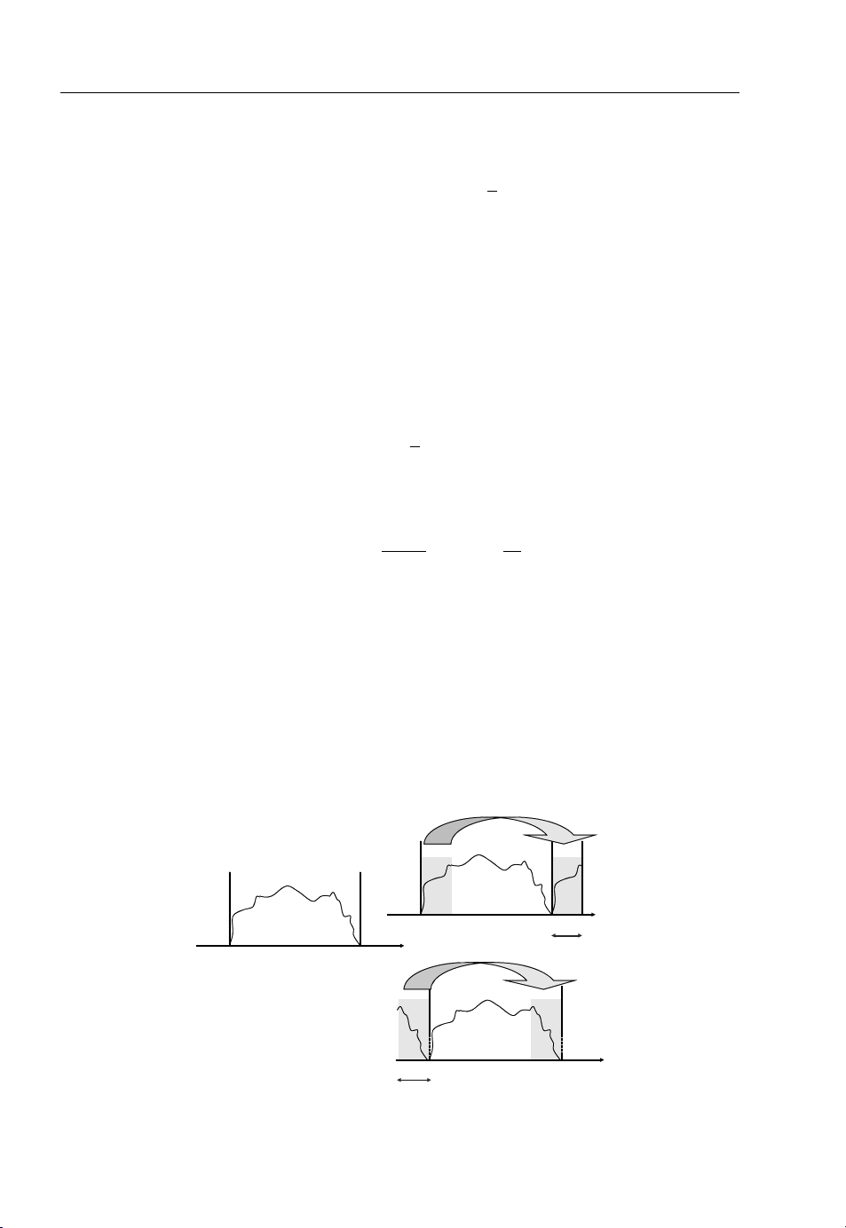
To minimise the OFDM system performance degradation due to PAPR, several techniques has been
explored each with varying degrees of complexity and performance enhancements. These schemes
can be divided into three general categories:
&
Signal Distortion Technique:
.
Signal Clipping
.
Peak Windowing
.
Peak Cancellation
&
Coding Technique
&
Symbol Scrambling Technique
The simplest way to mitigate the peak-to-average power ratio problem is to limit (clip) the signal such
that the peak level of the signal is always below the desired maximum level. However, this causes out of
band radiation and signal distortion. The effect of this clipping is analogous to the rectangular
windowing of the sample, which is equivalent to the spectrum of the desired signal being convolved
by the sinc-function (spectrum of the rectangular window) causing the spectrum regrowth in the side
bands and thus causing interference to the neighbouring channels. Simple clipping gives rise to spectral
growth in side bands. Therefore, to tame the spectral growth in adjacent bands, other windowing
functions with narrow bandwidth (such as Gaussian, Kaiser, Hamming and root raised cosine) have
been applied.
The goal of the signal distortion techniques is to reduce the amplitude of the data samples, whose
magnitude exceeds a certain threshold. The undesirable effect of signal distortion due to these can
be avoided by using the peak cancellation technique. In this method, a time-shifted and scaled reference
Page 31

Wireless Communications 21
is subtracted from the signal such that each subtracted reference function reduces the peak power of
at least one signal sample. A sinc-function could be used as a possible reference but this needs to be
spectrally limited. The sinc-function can be spectrally limited by applying the raised cosine window
function.
Researchers have looked into the applicability of coding techniques to mitigate the PAPR issue.
To achieve a smaller PAPR level the achievable code rate also becomes smaller. Although there are a
large number of code words available their implementation and properties for use as FEC codes (such as
minimum distance) may not be suitable for implementation. However, Wilkinson et al. [10] observed
that the largest portion of codes was Golay complementary sequences, which have a structured way of
implementing the PAPR reduction codes. The Golay complementary sequences are sequence pairs for
which the sum of autocorrelation function is zero for all delay shifts other than zero.
Another straightforward approach is the symbol scrambling technique. For each OFDM symbol, the
input sequence is scrambled by a certain number of scrambling sequences. The output signal with the
smallest PAPR is transmitted.
1.2.4 OFDMA
We note that the OFDM transmission uses all subcarriers for a packet time consisting of a number of
symbol durations. However, we can introduce a more flexible approach to allow each user to use the
partial frequency band (i.e., a number of subcarriers) and even partial packet time (i.e., a number of
symbol durations), so that multiple users can share this OFDM transmission, which is known as
orthogonal frequency division multiple access (OFDMA) or multi-user OFDM.
We have already discussed the OFDM as a multiplexing scheme, which provides better spectral
efficiency and immunity to multipath fading especially in a wireless environment. The OFDM also
lends itself to a simple implementation scheme based on highly optimised FFT/IFFT blocks. These
advantages can also be extended for multiple access schemes by assigning a subset of tones
(subcarriers) of OFDM to individual users. The allocation of subsets of tones to various users allows
for simultaneous transmission of data from multiple users allowing the sharing the medium. In this way,
it is equal to ordinary FDMA; however, OFDMA avoids the relatively large guard bands that are
necessary in FDMA to separate different users. An example of an OFDMA time-frequency grid
is shown in Figure 1.13, where seven users a to g each use a certain fraction – which may be different
for each user – of the available subcarriers. The blank time-frequency grids may be unused or occupied
Frequency
cce
d
d
e
e
e
ffg
a
a
a
a
g
b
g
b
b
g
b
a
a
a
a
b
b
b
b
cce
Time
d
d
e
e
e
ffg
cce
d
d
e
e
e
ffg
g
g
g
a
a
a
a
g
b
g
b
b
g
b
Figure 1.13 OFDMA with users a, b, c, d, e, f, g to share time-frequency grids
Page 32

22 Cognitive Radio Networks
by pilot signals. This particular example in fact is a mixture of OFDMA and TDMA, because each
user only transmits in one out of every four timeslots, which may contain one or several OFDM
symbols.
In the previous example of OFDMA, every user had a fixed set of subcarriers. It is a relatively easy
change to allow hopping of the subcarriers per timeslot. Allowing hopping with different hopping
patterns for each user actually transforms the OFDMA system into a frequency-hopping CDMA
system. This has the benefit of increased frequency diversity, because each user uses all of the available
bandwidth, as well as the interference averaging benefit that is common for all CDMA variants.
By using forward-error correction coding over multiple hops, the system can correct for subcarriers
in deep fades or subcarriers that are interfered with by other users. Because the interference and
fading characteristics change for every hop, the system performance depends on the average received
signal power and interference, rather than on the worst case fading and interference power. A major
advantage of frequency-hopping CDMA systems over direct-sequence or multicarrier CDMA systems
is that it is relatively easy to eliminate intra-cell interference by using orthogonal hopping patterns
within a cell.
OFDMA has been popular in wireless communication systems, such as IEEE 802.16e (OFDMA
version known as mobile WiMAX), IEEE 802.16m, 3GPP long-term evolution (LTE), etc. Hopping
OFDM is also used in well known ultra-wide band (UWB) communications (i.e., WiMedia), which is
going to be next phase system of the Bluetooth 3.0.
1.2.4.1 Radio Resource Allocation
A major difference of multiuser OFDM (OFDMA) from OFDM lies in radio resource allocation, which
is a typical network layer problem but has a strong relationship with physical layer transmission.
Since multiple users share the OFDM transmission in time domain (bits) and frequency domain
(subcarriers), the radio resource allocation algorithm to dynamically exploit best-use of time-frequency
grids can be viewed as the practical implementation of water-pouring to achieve Shannon capacity in
the ISI channel.
We assume there are totally K users, and the kth user has the data rate R
bit per OFDM symbol.
k
Depending on the number of bits assigned to a subcarrier, the adaptive modulator uses a corresponding
modulation and adjusts the transmit power level according to the combined subcarrier, bit, and power
allocation algorithm. We define c
as the number of bits of the kth user that are assigned to the nth
k,n
subcarrier. To model this problem, we do not allow more than one user to share one subcarrier or any
symbol/bit. That is, if c
k0;n
„ 0, c
number of bits per OFDM symbol for each subcarrier. We denote f
¼ 0 8k „ k0, while c
k;n
2f0; 1; ; Mg¼D and M is the maximum
k;n
(c) as the required power in a
k
subcarrier for reliable reception of cinformation bits/symbols when the channel gain isunity. In order to
maintain the required Quality of Service (QoS) at the receiver, the transmit power allocated to the nth
subcarrier by the kth user equals to
fkðc
Þ
k;n
¼
P
k;n
Our goal is to find the best assignment of c
k,n
given transmission rates of users and given QoS through f
and increasing with f
(0) ¼0, which perfectly matches practical modulation and coding schemes.
k
2
a
k;n
so that the overall transmit power is minimised under
(). We further require fk(c) convex
k
Mathematically,
N
K
X
X
fkðc
Þ
k¼1
k;n
2
a
k;n
*
P
T
¼ min
c
k;n
2D
n¼1
Page 33

Wireless Communications 23
subject to the following:
N
Constraint 1 : 8k 2f1; 2; ; K g; R
X
¼
n¼1
c
k;n
k
Constraint 2 : 8n 2f1; 2; ; Ng; if there exist k0with c
„ 0; then c
k0;n
¼ 0 8k „ k
k;n
0
1.2.4.2 Time and Frequency Synchronisation for Multiuser OFDM
Accurate demodulation of OFDM signals requires subcarrier orthogonality, and thus good synchronisation to maintain such orthogonality. By assuming perfect sample clock (i.e., integer sample-duration
misalignment in time), we try to estimate time and frequency offset of multiuser OFDM.
Statistical redundancy introduced by the cyclic prefix can provide the information about offset.
For one symbol received by the base station, we assume that N subcarriers constituting this symbol
are subdivided into M bands of subcarriers (collectively as the set M
). One transmitted OFDM symbol
m
in the mth band of subcarrier is
X
ðtÞ¼
S
m
n2M
where NT is duration of OFDM symbol without cyclic prefix; T
frequency offset relative to the receiver demodulation frequency; and «
j2pnt=NT
Xne
m
Tg< t < NT
g
is length of cyclic prefix; umis
is time offset relative to the
m
receiver symbol clock.
The received signal is
M 1
X
¼
rmðkÞ
m¼0
M 1
X
smðk mÞe
m¼0
j2pumk=N
þnmðkÞ
rðkÞ¼
where s
(k) is the transmitted signal.
m
We may use bandpass filters to separate subcarriers grouping if the estimator is good enough. For
the outputs of the mth filter, we may obtain the one-shot estimator
¼ arg max«fjrmð«ÞjrmRmð«Þg ð1:19Þ
^«
m
1
^
q
m
ffr
¼
2p
mð«m
Þ
where
« þ L 1
X
R
r
ð«Þ¼
m
rm¼
ð«Þ¼
m
1
2
SNRmþ1
rm*ðkÞrmðk þNÞ
k¼«
« þ L 1
X
jrmðkÞj2þjrmðk þNÞj
k¼«
SNR
m
SNR
2
2
s
S
m
¼
m
2
s
n
m
Page 34

24 Cognitive Radio Networks
Such an estimator is shown to be the joint maximum likelihood (ML) estimate of « and u if the output
of each filter
j2puk=N
rðkÞ¼~Sðk «Þe
þnðkÞð1:20Þ
where~SðkÞ are Gaussian distributed and uncorrelated except for the pairs of identical samples in the
cyclic prefix.
1.3 MIMO
One of the major challenges in physical layer communication design is to increase the spectral
efficiency to support broadband wireless communications over severe fading channels. From any
standard textbook in fundamental communications, such as [9] [11] one of the best ways to combat
fading is diversity to create independent communications channels. One straightforward way to create
diversity is through antennas, such as the well known receive diversity by multiple receiving antennas
with combining (where maximum ratio combining (MRC) is the optimal combining). Alamouti [13]
pioneered optimal transmit diversity for two transmit antennas in addition to receiver diversity, which
makes the communication channel into multiple-input and multiple-output (MIMO) by simultaneously
using transmit diversity and receive diversity. In the following text, three basic types of MIMO
technology will be introduced:
&
beamforming;
&
spatial multiplexing;
&
space-time codes.
Depending on the geometry of the employed antenna array, two basic multi-antenna approaches can be
considered: a beamforming approach for closely separated antenna elements (the inter-element
separation is at most l/2, where l is the carrier wavelength) or a diversity approach for widely
separated antenna elements (the typical inter-element spacing is at least a few l). In this chapter, we
explore the latter approach where the fading processes associated with any two possible transmitreceive antenna pair can be assumed to be independent. The fact that a MIMO system consists of
a number of uncorrelated concurrent channels has been exploited from two different perspectives.
First, from a pure diversity standpoint, one can enhance the fading statistics of the received signal
by virtue of the multiple available replicas being affected by independent fading channels. By sending
the same signal through parallel and independent fading channels, the effects of multipath fading
can be greatly reduced, decreasing the outage probability and hence improving the reliability of the
communication link.
In the second approach, referred to as spatial multiplexing, different information streams are
transmitted on parallel spatial channels associated with the transmit antennas. This could be seen as a
very effective method to increase spectral efficiency. In order to be able to separate the individual
streams, the receiver has to be equipped with at least as many receive antennas as the number of parallel
channels generated by the transmitter in general. For a given multiple antenna configuration, one may
be interested in finding out which approach would provide the best performance.
1.3.1 Space-Time Codes
Space-Time Coding (STC) is a hybrid technique that uses both space and temporal diversity in a
combined manner. There are two forms of STC namely Space-Time Block Code (STBC) and SpaceTime Trellis Code (STTC). STBC efficiently exploits transmit diversity to combat multipath fading
while keeping decoding complexity to a minimum. Tarokh et al. [19] show that no STBC can achieve
Page 35

Wireless Communications 25
full-rate and full-diversity for more than two transmit antennas, and proposed a 3/4 rate, full-diversity
code for four transmit antennas. A full-rate quasi-orthogonal (QO) STBC was proposed by Jafarkhani
[14] for four transmit antennas based on Alamouti’s orthogonal STBC. In this case, the transmission
matrix is given by
where A
, A34are the Alamouti codes. It is noted here that since the channel matrix of the QO-STBC is
12
A
A
12
¼
C
j
A
*
A
34
2
6
34
*
12
x
6
¼
6
4
x
x
x
1
*
2
*
x
3
x3x
2
*
x
x
1
*
x
4
x4x3x
3
4
7
*
*
x
7
4
3
7
*
*
5
x
1
2
*
x
1
2
ð1:21Þ
not full-rank, full-diversity gain cannot be attained. To achieve the full-diversity and full-rate (FDFR)
property, a new FDFR STC approach was recently proposed.
The Mixed (Hybrid Diversity and Spatial Multiplexing) mode combines diversity and spatial
multiplexing by transmitting from four transmit antennas, each space-time block coded with the
basic Alamouti scheme of order two. The transmission matrix of the space-time block coding for the ith
data stream, i ¼a, b, is given by
ðiÞ x2ðiÞ
x
A
i
ðiÞ*x1ðiÞ
x
2
*
1
¼
ð1:22Þ
To decode the data, Minimum Mean Square Error (MMSE) and Zero Forcing (ZF) receivers can be
employed. For the MMSE receiver, we assume that the transmitted matrix is [a
þ 1(k)]T, where a and b indicate different signal streams. First, the tap weight vector and decoding
b
2n
2n
(k), a
2n þ 1
(k), b2n(k),
layer order are determined. If the first decoding layer is a the procedure can be represented by
^
ðkÞ
a
^
a
2n þ 1
2n
ðkÞ
¼ decision
The interference from the original signal can be subtracted using^a
H
w
ðkÞ
1
H
w
2
ðkÞ
ðkÞ
y
n
ðkÞ and^a
2n
2n þ 1
ð1:23Þ
ðkÞ, and
accordingly, the other stream can be decoded as follows:
^
ðkÞ
a
0
y
ðkÞ¼ynðkÞ½h1ðkÞh2ðkÞ
n
^
ðkÞ
b
^
b
2n
2n þ 1
ðkÞ
¼ decision
h
ðkÞ
3
h
ðkÞ
4
2n
^
ðkÞ
a
2n þ 1
0
y
ðkÞ
:
n
ð1:24Þ
Note that for comparative purposes we can also employ Maximum Likelihood (ML) decoding
(explained in Section 1.3.1.1) to obtain the optimum performance, which was used as our baseline
reference.
In the following, we briefly review the employed spatial multiplexing scheme. The V-BLAST
architecture has been recently proposed for achieving high spectral efficiency over wireless channels
characterised by rich scattering. In this approach, one way of detection is to use conventional adaptive
antenna array (AAA) techniques, i.e., linear combining and nulling. Conceptually, each stream (i.e.,
layer) in turn is considered to be the desired signal, while regarding the remaining signals as
interference. Nulling is performed by linearly weighting the received signals so as to satisfy some
performance related criterion, such as ZF or MMSE. This linear nulling approach is viable, but superior
performance is obtained if nonlinear techniques are used. One particularly attractive nonlinear
alternative is to exploit symbol cancellation as well as linear nulling to perform detection. By using
symbol cancellation, the interference from the already-detected components is subtracted from the
received signal vector; reducing effectively the overall interference. Here we will consider ordered
successive interference cancellation with ZF and MMSE. Also, a ML decoding receiver will be used
as a reference.
Page 36

26 Cognitive Radio Networks
We assume that Hij(k) is the channel coefficientfrom the jthtransmit antenna to the ithreceive antenna
and w is white Gaussian noise with covariance matrix C
¼E[wwH] ¼s2IR. Then, the received signal
w
vector can be written as follows:
ðkÞ¼HðkÞxnðkÞþwðkÞð1:25Þ
y
n
where, the index k denotes the k
and w(k) is the (N
1) noise vector.
R
th
subcarrier, yðkÞ¼½y1ðkÞy
ðkÞT, xðkÞ¼½x1ðkÞx
N
R
N
R
ðkÞT,
1.3.1.1 Maximum Likelihood Decoding (Optimal Solution)
The ML detection of x(k) can be found by maximising the conditional probability density function and
this is equivalent to minimising the log-likelihood function:
where x(k)
^
xðkÞ¼min
2
all possible constellation sets.
fyðkÞHxðkÞgHfyðkÞHxðkÞg ð1:26Þ
xðkÞ
It is well known that ML decoding has a high complexity and thus suboptimal but practically
implementable solutions are considered next.
1.3.1.2 Ordered Successive Interference Cancellation (OSIC)
Instead of ML decoding approach, linear detection techniques can be used, i.e., zero-forcing and
MMSE. To improve the linear detection techniques, we try to decode according to received signal
strength, and extract the decoded signal from the received signal. This approach is referred to as
D-BLAST or V-BLAST according to the transmitted signal structure. For simplicity, we consider the
OSIC. The receiving operation of OSIC can be summarised as follows:
ü Step 1: Compute the tap weight matrix W.
ü Step 2: Find the layer with maximum SNR.
ü Step 3: Detection:
ðnÞ¼W
z
k
^
x
ðnÞ¼decision½zkðnÞ
k
H
k
yðnÞ
ü Step 4: Interference cancellation:
yðnÞ¼yðnÞ^h
ðnÞ
k
H ¼½h
; ; h
1
k 1
; 0; h
ü Step 5: Repeat Step 1 until all symbols are detected.
Zero-Forcing (ZF): The cost function can be expressed as:
¼fyðkÞH^xðkÞgHfyðkÞH^xðkÞg ð1:27Þ
J
ZF
Since J
is a convex function over^xðkÞ,^xðkÞcan be determined by using the minimum limit. Then,
ZF
the tap weight vector is given by
H
W ¼fH
Hg1H
k þ 1
H
; ; hT
ð1:28Þ
Page 37

Wireless Communications 27
Minimum Mean Square Error(MMSE): To take into account the noise variance the cost function can
be expressed as
¼ E½fyðkÞH^xðkÞgHfyðkÞH^xðkÞg ð1:29Þ
J
MMSE
Using a similar method to the ZF detection method, the weight vector results in
W ¼fH
H
H þs2Ig1H
H
ð1:30Þ
Note that the noise variance has to be estimated in order to use the MMSE approach.
1.3.2 Spatial Multiplexing Using Adaptive Multiple Antenna Techniques
Several authors have considered the diversity-spatial multiplexing problem. The fundamental tradeoff
between diversity and spatial multiplexing was explored by Zheng and Tse [15]. A scheme based on
switching between diversity and spatial multiplexing was proposed by Heath and Paulraj [16]. The
latter authors considered a fixed rate system in which the receiver adaptively selects one of the two
transmission approaches based on the largest minimum Euclidean distance of the received constellation. The receiver informs its selection to the transmitting via a one-bit feedback channel. To ensure a
fixed bit rate, the diversity scheme uses modulation with a higher order than that used by its counterpart
spatial modulation case. Skjevling et al. [17] presented a hybrid method combining both diversity and
spatial multiplexing. The proposed approach optimally assigns antennas to a given (fixed) transmission
scheme combining diversity and spatial multiplexing. Antenna selection is based either on full channel
feedback or long term statistics. Gorokhov et al. [18] studied the relationship between multiplexing
gain and diversity gain in the context of antenna subset selection, thereby extending the recent results by
Zheng and Tse [15].
1.3.3 Open-loop MIMO Solutions
Alamouti [13] developed a remarkable orthogonal full-diversity full-rate (FDFR) code for NT¼2
transmit antennas, requiring a simple linear decoder at the receiver. Tarokh et al. [19] proved that a
FDFR orthogonal code only exists for N
attaining full diversity but not full rate. A quasi-orthogonal full-rate code was proposed by Jafarkhani,
although full diversity gain cannot be attained. Based on space-time constellation rotation, Xin et al.
[20] and Ma et al. [21] proposed a FDFR encoder for an arbitrary number of transmit antennas. For an
even number of transmit antennas, Jung et al. [22] obtained coding gain with a FDFR space-time block
code by serially concatenating the Alamouti scheme with constellation rotation techniques. Although
the Alamouti based space-time constellation rotation encoder (A-ST-CR) can effectively achieve full
diversity and full rate, the decoding complexity is an issue and its practical implementation becomes
prohibitive, even for a small number of transmit antennas, e.g., N
computational complexity required by the maximum likelihood (ML) decoding algorithm.
In addressing the complexity problem, this chapter further extends these results by considering a
system based on the serial concatenations of a new rotating precoding scheme with the basic Alamouti
codes of order two. By a proper process of puncturing and shifting after the actual constellation-rotation
operation, the encoding process can be conveniently decomposed into rotation operations carried out
in a lower-order matrix space. The impact of this puncture and shift rotation coding scheme is very
significant atthe receiver,where due to the provided signal decoupling, the ML decoding is significantly
reduced. It is shown in this chapter that the proposed method attains the same performance as the
scheme presented with a substantial complexity reduction.
¼2 and proposed some space-time block codes for NT> 2
T
¼4. This is due to the high
T
Page 38

28 Cognitive Radio Networks
Researchers use a precoder based on the Vandermonde matrix to attain a FDFR system. After
multiplying the received signal x by the Vandermonde matrix, each component of vector r combines all
the symbols as can be observed in the next basic precoder equation:
r ¼ Qx ¼
2
1
1 a
6
1 a
6
1
6
ffiffiffi
p
6
4
1 a
4
1 a
a
0
1
a
1
1
a
2
1
a
3
3
2
3
2
2
3
x
a
0
2
a
1
2
a
2
2
a
3
1
0
7
6
7
3
x
7
6
7
2
1
7
6
7
7
6
7
3
x
5
4
5
3
2
3
x
4
3
3
r
1
6
7
r
6
7
2
6
7
¼
6
7
r
4
5
3
r
4
ð1:31Þ
where a
¼ expðj2pði þ1=4Þ=NÞ; i ¼ 0; 1; ; N 1.
i
Xin [20] and Ma [21] use a diagonal channel matrix after multiplying the information symbols by the
Vandermonde matrix. This linear precoding is referred to as the constellation rotating operation. Notice
that the coding advantage is not optimised, although the schemes successfully achieve FDFR. Jung [22]
improves the coding advantages by concatenating the constellation rotating precoder with the basic
Alamouti scheme, resulting in the following transmitted signals:
S ¼
2
r
r
1
r
2
*
*
r
2
1
0
0
0
0
6
6
6
4
r
r
3
0
0
7
0
0
7
7
5
r
3
4
*
*
r
4
3
ð1:32Þ
At the receiving end, the signal can be written as
2
3
y
1
6
7
y
6
7
2
y ¼
6
7
4
5
y
3
y
4
Note that since r
, r2, r3, r4already sums over x1x4through the Vandermonde matrix, each symbol
1
experiences the channel twice. At this point we can separate r
, r4)or(r1, r4and r2, r3), consequently the Vandermondematrix for the precoder needs not to be of size
r
2
2
h
1h2
6
h
1
6
2
ffiffiffi
p
¼
6
4
00h
2
00h
h
00
00
1
3
4
h
h
3
2
3
2
3
r
1
7
6
r
2
7
6
7
6
5
4
r
4
3
r
4
3
, r2, r3, r4into two parts i.e., (r1, r3and
1
n
1
7
6
7
n
7
6
7
2
þ
7
5
¼ Hr þ n ð1:33Þ
6
7
4
5
n
3
n
4
four, but smaller. Based on this observation, we can use a puncturing and shifting operation after the
constellation rotation process resulting in a new precoder:
r
¼
¼
1
r
3
r
2
r
4
r
1;3
r
2;4
"#
¼
1 a
2
1 a
1
ffiffiffi
p
"#
1 a
1
ffiffiffi
p
¼
1 a
2
1
0
1
2
1
1
1
3
x
1
x
3
x
2
x
4
r
or
r
1;4
2;3
¼
¼
r
1
r
4
r
2
r
3
"#
¼
1 a
2
1 a
1
ffiffiffi
p
"#
1 a
1
ffiffiffi
p
¼
1 a
2
1
x
0
1
x
3
1
x
1
1
x
2
1
4
2
3
ð1:34Þ
After puncturing and shifting, the encoder can be defined as
2
1 a
6
001a
1
6
ffiffiffi
p
6
4
1 a
2
001a
1
0
1
2
00
1
1
00
1
3
3
7
7
or
7
5
2
1 a
6
001a
1
6
ffiffiffi
p
6
4
001a
2
1 a
1
0
1
3
3
00
7
1
7
1
7
1
5
2
00
ð1:35Þ
Recently, Rajan et al. proposed a low decoding complexity (symbol by symbol decoding) improved
space-time code with full diversity for three and four transmit antennas configurations. The following
Page 39

Wireless Communications 29
is the format obtained modification to the transmission matrix:
2
þjy3x2þjy
x
1
6
þjy4x1jy
x
2
6
s ¼
6
4
00x
00x4þjy2x3jy
where x
cos u SiQsin u,yi¼siIcos u siQsin u and u ¼ tan1ð
i¼siI
take values from a QAM signal set.
4
3
3
00
00
þjy1x4þjy
3
7
7
7
5
2
1
1
Þ. The complex symbols s
3
ð1:36Þ
1.3.4 Closed-loop MIMO Solutions
In this section we explain the widely used closed-loop MIMO solutions, which consist of two parts, i.e.,
antenna grouping and codebook based schemes using feedback information from the mobile station.
1.3.4.1 Antenna Grouping
The rate 1 transmission code for 4 Tx BS in the IEEE802.16e is
A ¼
2
s
6
s
6
4
s
1
2
s
2
1
00s
00
00
3
00s4s
Note that this scheme does not achieve full diversity. Using the equivalent model
2
r
000
1
6
A ¼
0 r
6
4
00r
1
H
A
000r
3
7
7
5
s
4
3
3
7
00
7
5
0
2
2
ð1:37Þ
ð1:38Þ
i
If the BS can use channel state information, the performance of the existing matrix A approaches the
performance of the full diversity full rate STC:
jr1r2jð1:39Þ
2
Let d
be the corresponding minimum distance of the normalised unit energy constellation. The 2R-
min
QAM Euclidean distance equation d
arg min
antenna pair
2
¼ 12=ð2R1Þ will be used, corresponding to QAM modula-
min
tion for diversity. Using this Euclidean distance equation, we can estimate the error probability as
r
ffiffiffiffiffiffiffiffiffiffiffiffiffiffiffi
E
s
NeQ
P
e
2
where d
neighbours in the constellation, and can be found for each proposed mapping scheme based on the
channel coefficient matrix HQðxÞ¼
For STC, the minimum distance of the diversity constellation at the receiver can be shown to be
is the squared Euclidean distance of the received signal and Neis the number of nearest
MIN
ffiffiffi
p
1
d
2
MIN
ðHÞ
erfc x=
2
min jjH jj
2
2
ða ; b Þ; jjH jj
F
2
d
MIN
N
0
, where erfc is the complementary error function.
2
ðc ; d Þ
F
N
T
2
d
min
ð1:40Þ
ð1:41Þ
Page 40

30 Cognitive Radio Networks
where (a, b) and (c, d) are the antenna grouping index and kHkFis the Frobenius norm of matrix H.
The details for derivation follow the derivation procedure of the maximum SNR criterion for code
design. Figure 1.14 shows the system block diagram, which makes use of a grouper to select the antenna
pair based on feedback channel information from the MS.
Tx. ant ennas
[
s
Matrix
A1 or A2
r
or A3
s
s
[
]
21Ts
)()(
f
1
43Ts
)()(
]
f
2
2bits Feedback
Alamouti
Encoder
Alamouti
Encoder
Figure 1.14 System block diagram
The performance of the proposed scheme can outperform the conventional STC without antenna
grouping by 3.5 dB.
The rate 2 transmission code for four transmit antennas in the current standard is
B ¼
2
s
1
6
s2s
6
4
s3s
s4s
s
1
3
2
4
s5s
s6s
s7s
s8s
3
7
7
8
7
5
5
6
ð1:42Þ
At the mobile, the optimum transmission matrix is determined based on the following criteria. Let y
be the received signal at the ith symbol time at the rth receive antenna, and let h
denote the channel
i,r
parameter between the tth transmit and rth receive antenna. When the number of receive antennas is
two, the received signal can be represented as
r,i
y ¼ XðHWÞs þv ð1:43Þ
where y ¼
*
y
1;2
y
2;1
y
1;1
T
*
y
, s ¼ s1s2s3s
2;2
½
h
H ¼
1;1h2;1h3;1h4;1
h
1;2h2;2h3;2h4;2
T
, v is the noise vector,
4
and X() is a function of a 2-by-4 input matrix which is defined as
2
abcd
X
ef gh
abcd
*
6
b
a*d*c
6
¼
4
ef gh
*
f
e*h*g
3
*
7
7
5
*
ð1:44Þ
Page 41

Wireless Communications 31
At the mobile station, the index of the transmission matrix Bq is determined based on the following
criteria:
q ¼ arg min
l¼1;;6
absðdet ðH
Þþdet ðH
l;1
ÞÞ
l;2
ð1:45Þ
where H
is the first two columnsof HWland H
l,1
is thelast two columns of HWl. Note that the antenna
l,2
grouping matrix selection rule in Equation (1.45) is equivalent to the following rule:
hi
q ¼ arg min
l¼1;;6
trace ðXðHWlÞÞHXðHWlÞ
1
ð1:46Þ
Alternative criteria for the antenna grouping can be applied to determine the antenna group index.
For example, minimise BER, minimum mean square error, etc.
1.3.4.2 Codebook based Closed-Loop MIMO
The codebook is employed in the feedback from the MS (mobile station) to the BS (base station). The
MS learns the channel state information from the downlink and selects a transmit beamforming matrix
for the codebook. The index of the matrix in the codebook is then fed back to the BS. Each codebook
corresponds to a combination of N
antennas, available data streams and bits for the feedback index respectively. Once N
determined in the MS, the MS will feed back the codebook indexes, each of N
bit index, the BS will look up the corresponding codebook and select the matrix (or vector) according
N
i
and Ni, where Nt,Nsand Niare the numbers of BS transmit
t,Ns
t,Ns
bits. After receiving a
i
and Niare
to the index. The selected matrix will be used as the beamforming matrix in MIMO precoding.
1.3.5 MIMO Receiver Structure
Let us consider uncoded MIMO transmission as
y ¼ Hx þn ð1:47Þ
where n is a spatio-temporally white circularly symmetric complex Gaussian noise vector with zeromean and variance in each component, and H is the channel matrix.
ML detection of x gives
^
x ¼ arg minxky Hxk
2
where h
M
X
¼ arg min
x
i¼1
is the (i, j) th component of the matrix H. Such a complexity grows exponentially with M
i,j
R
jyi
M
X
j¼1
T
2
h
j
i;jxj
and Q (Q being bits per symbol in modulation).
1.3.5.1 Linear Receivers
The basic idea is to pre-process the received signal by linear transform
~
y Ay ¼ AHx þAn
so that AH is close to a diagonal matrix. The immediate approach to select the pre-processing matrix is
zero-forcing receiver (ZF) to remove the off-diagonal elements of AH.
~
¼ HþyHþ: Moore-Penrose pseudo-inverse of H
y
ZF
T
Page 42

32 Cognitive Radio Networks
1.3.5.2 LMMSE Receiver
Another approach is to minimise jointly the effects of off-diagonal elements of AH and of the filtered
noise An, which is known as linear minimum mean-square error (LMMSE):
~y
LMMSE
¼ HHH þ
1
N
0
I
E
HHy
where E is the average energy of one component of x, and I is the M
TMT
identity matrix.
Linear receivers usually enjoy system complexity, at the price of poorer performance, especially
T¼MR
.
M
1.3.5.3 Decision-feedback Receivers
The pre-processing of decision-feedback detection involves the decomposition of the channel matrix
H into the product form
H ¼ QR
For the purpose of simplicity, we assume that M
. Then, QHQ ¼ I
RMT
triangular. Using this decomposition, the transformed observation vector~y Q
~
y Rx þ~n
where~n Q
H
n retains the statistical property of n. To minimise mðxÞjjy Hxjj
and R
M
T
H
y has the form
is upper
MTM
T
2
is therefore to
F
minimise
~
mðxÞjjy Rxjj
2
From the structure of R, the detection algorithm is
detect x
us x
by minimising j~y
M
T
to detect x
M
T
by minimising
MT1
j~y
MT1
r
M
T
r
MT;1;MT1rMT;1;M
MT;M
x
M
T
T
j2and then
^
j2þj~y
x
M
T
T
r
MT;;M
M
T
2
^
j
x
M
T
T
This algorithm is clearly prone to error propagation.
1.3.5.4 Sphere Detection
The sphere detection algorithm (SDA) achieves performance close to ML, with lower complexity.
The basic idea is to conduct the search for optimum x within a small subset of potential candidates.
Typically, the search is constrained to a hyper-sphere centred at y of radius r
2
2
jjy Hxjj
r
If r ! ¥, it is just ML detection. The reduction of complexity is determined by appropriate selection
of r.
SDA can be commonly implemented by considering a tree as shown in Figure 1.15, in which the
bottom leaves correspond to all possible vectors x, with the components of x labelling branches from
bottom to top.
Again,~y ¼ Q
~
mðxÞjjy Rxjj
H
y, and ML detection is equivalent to traversing the tree by computing the metric
2
for all possible branches and retaining the minimum value. In other words, SDA
reduces the number of branches to be checked by proper pruning of the tree. The operating algorithm
can be summarised as follows:
Page 43

Wireless Communications 33
x
3
x
2
x
1
Figure 1.15 SDA for a MIMO with MT¼3 and quaternary modulation
1. Use the decision feedback receiver to obtain a preliminary estimate^x of x, and to compute the
corresponding metric~mð^xÞ^y Rx
kk
2
.
2. Such a value is set as the squared radius of the sphere. The tree is now traversed, depth-first, from top
to down, and the metric computed incrementally by adding one-by-one:
M
T
X
^
y Rxkk
2
¼
i¼1
j^yiðRxÞij
2
3. Whenever the accumulated partial sum at a node is larger than (or equal to)~m^xðÞ, there is no
checking of the leaves below the node (i.e., no further consideration).
4. If a new x is found with metric smaller than~m^xðÞ, then it replaces x in the rest of the algorithm
(i.e., shrinking the hyper-sphere in ML search).
1.3.5.5 MIMO Receivers for Uncoded Signals
Detection of uncoded signals at the output of a MIMO channel can be viewed as a special case of
equalisation for a general channel.
Consider a MIMO channel with M
transmit and MRreceive antennas. The input-output relationship
T
of the channel can be described by the conditional probability density function
M
R
Y
2
where f ðy
jxÞ¼e
j
jyjhjxj2=N
f ðyjxÞ!
f ðyjxÞ!e
0
and hjis the jth row of H.
M
T
Y
jjy Hxjj
f ðxiÞf ðyjx1x
i¼1
=N
0
F
¼
f ðyjjxÞ
j¼1
M
T
Y
Þ¼
M
T
i¼1
f ðxiÞ
M
Y
j¼1
R
f ðyjjxÞ
To avoid the complexity of iterative algorithm, we may consider suboptimum MIMO receivers by
1. pre-processing the received signal to limit the effects of spatial interference:
~
y AðHÞy ¼ AðHÞHx þAðHÞn
2. and exchanging the message in a simplified version;
3. and detection consists of a single sweep of a finite number of steps.
Page 44

34 Cognitive Radio Networks
We now recall
~
¼ Hþy
y
ZF
to yield
~
y ¼ x þH
þ
n
with noise enhancement. Or, we may use LMMSE to minimise MSE
2
EfjjAy xjj
AðHÞ¼ H
H
H þ
g
F
1
N
0
E
s
H
I
H
Since the off-diagonal terms in A(H)H are small, the resulting detection algorithm is based on the
approximation
jx1; x2; x
f ðy
i
Both ZF and LMMSE structures perform well if M
Þf ðyijxiÞ
M
T
MT.
R
1.3.5.6 Nonlinear Processing
The well-known V-BLAST falls into a class of suboptimum receivers based on the following
operations:
&
Nulling of spatial interference: This is achieved by modifying the pre-processing operation.
&
Cancellation of spatial interference: This is obtained by simplifying
jxi; x
f ð~y
i
in a sequential way for i ¼ M
&
Ordering: Since V-BLAST is prone to error propagation, antenna ordering may significantly affect
; ; x
i þ 1
1; MT2; ; 1 where^x denotes a decision based on x.
T
Þf ð~yijxi;^x
M
T
i þ 1
; ;^x
Þ
M
T
receiver performance.
1.4 Multi-user Detection (MUD)
Actually,the initial MIMO system can be a CDMA system asFigure 1.16 with multiple transmitters and
multiple receivers. However, most CDMA systems adopt a single-user receiver structure and treat other
users’ signals as co-channel interference. Following Verdu’s and Poor’s [23] efforts to explore optimal
reception of CDMA signals, a new branch of communication theory, known as multi-user detection
(MUD), has been developed.
1.4.1 Multi-user (CDMA) Receiver
CDMA system performance is dominated by MAI conventional correlation receivers and cannot
optimally detect signals in this situation.
Each user transmits digital information at the same data rate 1/T. The bipolar data stream of the kth
user is
T
¼½bkðMÞ; ; bkð0Þ; ; bkðMÞ
b
k
Page 45

Wireless Communications 35
(t)
Source
(m)
d
k
b1(m)
−→
1110→
Transmitter #1
c1(t )
….
b
k
Spread
Spectrum
Modulation
(t )
c
k
+
Channel
r (t )
bk(m)
Transmitter #K
c
(t )
k
Figure 1.16 CDMA system
The transmitted signal of the kth user is given by
M
X
ðtÞ¼
m¼M
T
normalised condition
c
ð
T
1
T
0
where t
is time delay for the k th user.
k
Assume short code N ¼ G
x
h
¼
p
T
The received energy per bit is
ð
T
2
E
b
c
k
k
0
The received waveform is therefore
rðtÞ¼
K
X
k¼1
p
ffiffiffiffiffiffiffi
E
ck
M
X
m¼M
bkðmÞckðt mT tkÞ
2
c
ðtÞdt ¼ 1
h
2
ðmÞc
ðtÞdt ¼ E
k
c
k
bkðmÞckðt mT tkÞþnðtÞ
where t
< T and tk¼0 for synchronous case.
k
For a one-shot signal (m ¼0)
The cross correlation of signature is
ðjÞ¼
r
ln
l ¼ 1; 2; ; K
n ¼ 1;2; ; K
j ¼M; ; 0; ; M
rðtÞ¼
ð
1
T
K
X
ffiffiffiffiffiffiffi
p
E
k¼1
Tlþðm þ1ÞT
þmT
T
l
ð0ÞckðtÞþnðtÞ
b
c
k
k
clðt tlÞcmðt þjT tnÞdt
Page 46

36 Cognitive Radio Networks
A conventional receiver making one-shot decisions is not optimal since information on interference
is ignored. While developing optimum detection, we assume that signature waveforms, time delays,
phase shifts, amplitudes and numbers of users are available.
Optimum receivers could select the following bit sequence
^
b ¼
2
^
b
ðMÞ ^b1ðMÞ
1
6
.
6
.
4
.
^
b
ðMÞ ^bkðMÞ
k
3
7
.
7
.
5
.
which maximises the conditional probability
P½^b rðtÞj
If we assume the transmitted bits are independent and equally probable, then it is equivalent to
maximising
PrðtÞj^b
¼ c exp
0
@
"#
2s
ð
T
1
ykðtÞ
2
0
n
K
X
k¼1
ffiffiffiffiffiffiffi
p
^
b
ð0Þ
E
k
c
c
k
k
ðtÞ
1
2
A
dt
; t 2 0; T½
This optimisation can be achieved by the Viterbi algorithm or in a form of maximum likelihood
sequence detection (Figure 1.17). Unfortunately, it has exponential complexity (i.e., complexity
growing exponentially with the number of users) as an NP-hard problem.
τ
mTjTc++
r (t)
ϕ
]cos[w
+t
1
c
X
c
X
Matched
Filter
ϕ
]cos[w
+t
k
Matched
Filter
1
X
(m)1c
τ
mTjTc++
k
X
(m)
c
k
N−1
∑
j = 0
N−1
∑
j = 0
(⋅)
(⋅)
y1(m)
y
(m)
k
Viterbi
Algorithm
ˆ
(m)
b
1
(m)ˆb
k
Figure 1.17 Optimal receiver
Let us look at the two-user case: T1¼0, T2T. The matched filter outputs at the mth sampling instant
are given by
ð
ðm þ 1ÞT
ðmÞ¼
y
1
y
ðmÞ¼
2
1
T
mT
ð
ðm þ 1ÞT þ T
1
T
mT þT
rðtÞc1ðtÞdt
2
rðtÞc2ðt T2Þdt
2
Page 47

Wireless Communications 37
where
M
X
p
rðtÞ¼
y
ðmÞ¼
1
ðmÞ¼
y
2
b
_
1
b
_
2
ffiffiffiffiffiffiffi
E
p
ffiffiffiffiffiffiffi
E
ð_
¼z
1
p
ffiffiffiffiffiffiffi
E
ð_
¼z
2
¼½b1ðm1Þ;b1ðmÞ;b1ðmþ1Þ
b
¼¼½
2
b1ðiÞc1ðtiTbÞþ
c
1
c
b
c
b
i¼M
b
1
;_
1
b
2
;_
1
ðmÞþ
1
b
Þþn1ðmÞ
2
ðmÞþ
2
b
Þþn1ðmÞ
2
p
p
ðm1Þ;b1ðmÞ;b1ðmþ1Þ
ffiffiffiffiffiffiffi
b
E
ðm1Þr12ð1Þþ
c
2
2
ffiffiffiffiffiffiffi
b
E
ðm1Þr21ð1Þþ
c
1
1
p
ffiffiffiffiffiffiffi
E
M
X
b2ðiÞc2ðtiTbt2Þ
c
2
i¼M
p
ffiffiffiffiffiffiffi
b
E
c
2
p
ffiffiffiffiffiffiffi
b
E
c
1
ðmÞr12ð0Þþ
2
ðmÞr21ð0Þþ
1
p
ffiffiffiffiffiffiffi
b
E
ðmþ1Þr12ð1Þþn1ðmÞ
c
2
2
p
ffiffiffiffiffiffiffi
b
E
ðmþ1Þr21ð1Þþn2ðmÞ
c
1
1
The resulting receiver is shown as Figure 1.18.
Figure 1.18 Tap delay line model for synchronous CDMA
Ð
T þt
k
Note: rkhðjÞ¼
1
T
chðt tkÞckðt þjT tcÞdt ¼ d
t
k
J
1.4.2 Suboptimum DS/CDMA Receivers
Since the optimal multi-user receiver has complexity exponentially to the number of users, it is
practically impossible to implement and suboptimal solutions are very much needed.
1.4.2.1 Decor-relating Receiver
The results for the two-user case can be easily generalised for a k-user system
y ¼ RAB þn
where R is the cross correlation matrix [r
A ¼
b ¼
]
ij
p
ffiffiffiffiffiffiffi
2
E
c
1
6
4
2
6
4
b
.
.
.
0
b
ðMÞ b1ðMÞ
1
.
.
.
ðMÞ bkðMÞ
k
p
0
ffiffiffiffiffiffiffi
E
3
7
5
c
k
3
7
.
.
5
.
Page 48

38 Cognitive Radio Networks
Then,
1
R
y ¼ Ab þR1n
Ignoring the noise term t
results in a scale transmitted sequence at the right-hand side. The decor-
0
relating receiver is based on the prior linear transformation, which consists of
&
matched filter bank as the front-end processor producing y;
&
decor relater computing R
1
.
The advantages for decorrelating the multi-user receiver are:
&
low complexity (linear in most cases);
&
no need of receiving amplitude and thus near-far resistant.
1.4.2.2 Interference Canceller (IC)
The operation of the interference canceller is based on successive cancellations of interference from the
received waveform (Figure 1.19). It cancels the strongest detected signal and consists of
ffiffiffiffiffiffiffi
1. ranking the user signals
p
ffiffiffiffiffiffiffi
E
ffiffiffiffiffiffiffi
p
>
c
1
p
ffiffiffiffiffiffiffi
E
>
c
2
E
c
> >
3
2. detecting the strongest user by the conventional receiver;
3. regenerating the strongest user spread spectrum signal^x
p
ðtÞ¼
k
E
;
c
k
ffiffiffiffiffiffiffi
p
^
E
ðtÞckðtÞ;
b
c
k
k
4. cancelling the strongest interferer;
5. repeating until all user signals done.
Figure 1.19 Interference canceller
If such cancellation proceeds serially, we call it ‘successive interference cancellation’ (SIC). It can also
be done in parallel, and we call such schemes ‘parallel interference cancellation’ (PIC).
1.4.2.3 Adaptive MMSE Receiver
Adaptive minimum mean square error (MMSE) receivers do not require signature, timing and carrier
phase information aboutinterferes, butonly the timing and carrierphase ofthe desired user (Figure 1.20).
Page 49

Wireless Communications 39
r(t)
X
]cos[w
+t
ϕ
1
c
X
]cos[w
+t
ϕ
k
c
Adaptive
Filter
Adaptive
Filter
Adaptive
Filter
Adaptive
Filter
Decision
Training
Sequence
Decision
Training
Sequence
ˆ
(m)
b
1
ˆ
(m)
b
k
Figure 1.20 Adaptive MMSE receiver
The timing recovery of the receiver is greatly simplified by the fractional filter, which makes the
detecteddesired signal insensitive to timedifferences.The adaptive FSE filterconsistsof 2L þ 1 taps. The
tap coefficients a
are determined by minimising the MSE between filter output and a known sequence.
l
The sampled filter input is
M
K
X
rðmT
Þ¼
f
X
i¼M
k¼1
p
ffiffiffiffiffiffiffi
E
b
ðmTfiT tkÞþnðmTfÞ
c
kck
k
The filter output, which is only calculated at T seconds apart, is
L
yðmTÞ¼
X
alrðmT lTfÞ
l¼L
Let us consider user 1 with no specific notation. The MSE is
2
« ¼ Eðl
Þ¼E ½yðmT ÞbðmÞ
m
no
¼ E ½a
a
¼ða
L
r ¼½rðmT þLTfÞ; ; rðmT Þ; ; rðmT LTfÞ
« ¼ a*Daða
where D ¼ Eðrr*Þ, f ¼ E½b*ðmÞr, s
A direct calculation of the lth element, f
no
T
r bðmÞ
; ; aLÞ
2
b
2
T
*
*
fþf
aÞs
¼ E½jbðmÞj2
, of the single-user channel vectorfis
e
2
T
2
b
¼ E½bðmÞrðmT þlTsÞ ¼ E½jbðmÞj2cðlTsÞ
f
e
The optimum tap setting is
a
¼ 1 f*D1f
opt
Please note thatf, D might not be available in practical cases. It makes LMMSE of great interest.
As a matter of fact, the suboptimal MUD can simply share the same principle of MIMO receiver
structure. Please recall that
y ¼ Hx þn
Page 50

40 Cognitive Radio Networks
It is just as equivalent to the MUD problem as
y ¼ RAb þn
Therefore, suboptimal MUD and MIMO receivers share the same principle in the receiver structure
if we treat H and RA equivalently.
References
[1] R.W. Chang, ‘Synthesis of Band-Limited Orthogonal Signals for Multichannel Data Transmission’, Bell Systems
Technical Journal, 45, 1960, 1775–1796.
[2] B.R. Saltzberg, ‘Performance of an Efficient Parallel Data Transmission System’, IEEE Transactions on Communi-
cation, 15(6), 1967, 805–811.
[3] S.B. Weinstein, P.M. Ebert, ‘Data Transmission of Frequency Division Multiplexing Using the Discrete Frequency
Transform’, IEEE Transactions on Communication, 19(5), 1971, 623–634.
[4] A. Peled, A. Ruiz, ‘Frequency Domain Data Transmission Using Reduced Computational Complexity Algorithms’,
Proceedings of the IEEE International Conference on Acoustics, Speech, and Signal Processing (ICASSP’80),
Denver, USA, 1980, pp. 964–967.
[5] T. Pollet, M. Peeters, ‘Synchronization with DMT Modulation’, IEEE Communications Magazine, April 1999,
80–86.
[6] T.Pollet, P. Spruyt, M. Monenclaey, ‘The BER Performance of OFDM Systems Using Non-Synchronized Sampling’,
IEEE Global Telecommunications Conference, 1994, pp. 253–257.
[7] J.M. Paez-Borrallo, ‘Multicarrier Vs. Monocarrier Modulation Techniques: An Introduction to OFDM’, BWRC
Retreat, 2000.
[8] T. Pollet, M. Van Bladel, M. Monenclaey, ‘BER Sensitivity of OFDM Systems to Carrier Frequency Offset and
Wiener Phase Noise’, IEEE Transactions on Communication, 43(2), 1995, 191–193.
[9] J.G. Proakis, Digital Communications, 4th edition, McGraw-Hill, New York, 2000.
[10] T.A.Wilkinson, A.E. Jones, ‘Minimization of the Peak-to-Mean Envelope Power Ratio of Multicarrier Transmission
Schemes by Block Coding’, Proceedings of IEEE VTC ’95, July 1995, pp. 825–829.
[11] K.C. Chen, Principles of Communications, River, 2009.
[12] R. Van Nee, R. Prasad, OFDM for Wireless Multimedia Communication, Artech House Publishers, 2000.
[13] S.M. Alamouti, ‘A Simple Transmit Diversity Technique for Wireless Communications’, IEEE Journal on Selected
Areas in Communications, 16(8), 1998, 1451–1458.
[14] H. Jafarkhani, ‘AQuasiorthogonal Space-Time Block Code’, IEEETransactions onCommunications, 49, 2001, 1–4.
[15] L. Zheng, D.N.C Tse, ‘Diversity and Multiplexing: A Fundamental Tradeoff in Multiple-Antenna Channels’, IEEE
Transactions on Information Theory, 49, 2003, 1073–1096.
[16] R.W. Heath Jr., A. Paulraj, ‘Switching Between Spatial Multiplexing and Transmit Diversity Based on Constellation
Distance’, Proceedings of Allerton Conference on Communication, Control and Computing, October 2000.
[17] H. Skjevling, D. Gesbert, N. Christophersen, ‘Combining Space Time Block Codes and Multiplexing in Correlated
MIMO Channels: An Antenna Assignment Strategy’, Proceedings of Nordic Signal Processing Conference
(NORSIG), June 2003.
[18] A. Gorokhov, D. Gore, A. Paulraj, ‘Diversity Versus Multiplexing in MIMO System with Antenna Selection’,
Allerton Conference, October 2003.
[19] V. Tarokh, N. Seshadri, A. Calderbank, ‘Space-Time Codes for High Data Rate Wireless Communications:
Performance Criterion and Code Construction’, IEEE Transactions on Information Theory, 44, 1998, 744–765.
[20] Y. Xin, Z. Wang, G.B. Giannakis, ‘Space-Time Diversity Systems Based on Linear Constellation Precoding’, IEEE
Transactions on Communications, 49, 2001, 1–4.
[21] X. Ma, G.B. Giannakis, ‘Complex Field Coded MIMO Systems: Performance, Rate, and Trade-offs’, Wireless
Communication and Mobile Computing, 2002, 693–717.
[22] T.J. Jung, K. Cheun, ‘Design of Concatenated Space-Time Block Codes Using Signal Space Diversity and the
Alamouti Scheme’, IEEE Communication Letters,
[23] S. Verdu, Multiuser Detection, Cambridge University Press, 1998.
7, 2003, 329–331.
Page 51

2
Software Defined Radio
2.1 Software Defined Radio Architecture
Many different wireless communication systems exist and they are widely used for different purposes
and application scenarios. Figure 2.1 illustrates some popular wireless communications international
standards, ranging from body area networks, personal area networks, local area networks and
metropolitan area networks, to wide area networks, with different application scenarios and optimised
system parameters. As a matter of fact, for the cellular type system alone, we may have a variety of
systems in use, such as legacy GSM, GPRS and EDGE, 3GPP wideband code division multiple access
(WCDMA) with its update versions of HSDPA and HSUPA, and the upcoming 3GPP long-term
evolution (LTE), and that is just considering air-interface technology. Figure 2.2 depicts possible
cellular air-interface technology migration and we can easily observe a variety of systems in use or in
future use, including time division multiple access (TDMA), code division multiple access (CDMA)
and orthogonal frequency division multiple access (OFDMA). These air-interface technologies
may co-exist in different geographical regions, and may co-exist simultaneously at the same location.
A flexible realisation of terminal devices to allow users to appropriately use wireless communications
is definitely essential.
Since the early days of electronic communications, however, typical (wireless) communication
systems have been implemented by certain dedicated hardware and likely dedicated application
specific integrated chips (ASIC) based on specific communication system parameters designed for use.
It is quite different from the way that we use computers to run different applications and programs on
the same computing facility. Software defined radio (SDR) that allows multiple systems realised
by programs to run on a single hardware platform is therefore attractive under such scenarios (multiple
co-existing systems in the same location or globally).
For a state-of-the-art terminal device, there are usually three types of processors for host featured
applications and wireless communication/networking purposes:
&
Microprocessor: Weusually have a host processor for each terminal, such as in notebook computers,
to serve the fundamental applications such as programming or executionof (multimedia) application
software.
&
Embedded processor(s): Embedded processors typically run networking functions of a device,
and sometimes applications with/without the host processor.
&
Digital signal processor(s) (DSP): When we execute wireless communications or extensive
multimedia features such as audio and video, we usually adopt digital signal processors to facilitate
Cognitive Radio Networks Kwang-Cheng Chen and Ramjee Prasad
©
2009 John Wiley & Sons Ltd. ISBN: 978-0-470-69689-7
Page 52

42 Cognitive Radio Networks
IS-95
WAN
IEEE 802.20
IEEE 802.16
(mobile WiMAX)
IEEE 802.11
MAN
LAN
UMTS, GPRS
ETSI
HIPERACCESS
ETSI
HIPERLAN
PAN
IEEE 802.15
Bluetooth
Wireless USB (UWB)
BAN
Figure 2.1 Global wireless communication standards
CDMA2000
(3GPP2)
TDD
IEEE 802.16e
Mobile WiMAX
EvDO
IEEE 802.16m
UMB
3GPP
?
IMT-Advanced
?
4G
TD-SCDMA TD-SOFDM
GSM
GPRS
EDGE
WCDMA
(3GPP)
HSPA
(HSDPA/
HSUPS)
3G LTE
NB/TDMA
CDMA/FDD
CDMA/TDD
OFDMA
Figure 2.2 Air-interface technology migration of cellular systems
functions. DSP is a special purpose processor offering tremendous processing power for rather
dedicated applications.
In other words, to execute wireless communications, we usually use DSPs for physical layer baseband
implementation, and embedded processors for networking functions and control. SDR hardware
structure can be summarised as shown in Figure 2.3. Antenna, PA and RF are just like conventional
wireless communication hardware, with an analogue-to-digital converter (ADC) to transform analogue
waveform into digital samples for the receiver, and DAC for the transmitter path. The flexibility of SDR
primarily lies in a programmable baseband section. For SDR operating at multiple frequency bands, we
may either use a set of dedicated RFs or a tunable wideband RF covering several frequency bands.
Page 53

Software Defined Radio 43
BUS
Antenna
(Array)
RF
& PA
A/D
D/A
ROM
Embedded
Processor
& Digital
Signal
Processor
System &
Frequency
Selection
External
Control &
RAM
MicroProcessor
Multimedia
I/O
Figure 2.3 Hardware structure of SDR device
For physical-layer communication transceiver (transmitter and receiver) realisation, the RF segment
and PA are handled by analogue circuits, and the baseband segment is implemented by DSP for SDR.
The major design efforts are to transform each baseband communication block into algorithms
computed by DSP programming. Higher layer networking functions are usually realised by embedded
processor programs. Device (host) microprocessor and/or application processors handle multimedia
and user interface applications (see Figure 2.4).
DSP Algorithms:
Real-Time
Protocol Stack:
Applications:
RF
& PA
A/D
Mod/Demod
Codec
Synchronization
RAKE Rx.
Equalization
MIMO Processing
Channel Est.
Layer-1 Driver
MAC
Link Control
Radio Resource
Logic Channel
Network Mgt.
QoS
Security
OS
User-Interface
Key M gt .
Multimedia
Appl. S/W
D/A
DSP &
HW
Embedded
Processor
Micro-
Processor
Figure 2.4 Software structure of SDR device
2.2 Digital Signal Processor and SDR Baseband Architecture
In contrast to typical general-purpose processors dealing with data manipulations, digital signal
processors (DSP) target mathematical calculations for special-purpose applications such as control,
media processing, communications, etc., operating at a much higher operation rate. Many state-of-theart (wireless) communication products are implemented by DSPs.
Typical general-purpose processors use the well-known Von Neumann machine architecture
in which memory is shared by instructions and data through a single data bus. DSP typically adopts
the so-called Harvard architecture of separate program memory and data memory through a dedicated
Page 54

44 Cognitive Radio Networks
program memory bus and data memory bus. We may further add an instruction cache into the CPU
and an I/O controller as a super Harvard architecture for DSP. Figure 2.5 illustrates these three
architectures.
Memory for
Data &
Instructions
Von Neumann Machine
Program
Memory
for
Instructions
Harvard Architecture
Program
Memory
for
Instructions
Super Harvard Architecture
Address Bus
Data Bus
PM Address Bus
PM Data Bus
PM Address Bus
PM Data Bus
CPU
CPU
CPU
Instruction
Cache
DM Address Bus
DM Data Bus
DM Address Bus
DM Data Bus
Data
Memory
for
Data only
Data
Memory
for
Data only
I/O Controller
Figure 2.5 Processor architecture
Since the signal waveforms for multimedia or communications are usually analogue, analogue-todigital conversion is required to encode the analoguewaveform into digital samples for DSP to process.
Digital signal processing using DSP has two categories: floating-point and fixed-point, based on the
sample format to store and to manipulate. Fixed-point DSP represents each sample by a fixed number of
bits, usually 16, 32 or 64 but 24 in some DSPs. For 16-bit fixed-point DSP, each sample has2
16
¼65,536
possible ‘unsigned integer’ values. Floating-point DSP usually uses 32 bits or even 64 bits to represent
each sample. In the common format of 32-bit floating-point, the largest and the smallest represented
numbers are 3.4 10
38
and 1.3 10
38
respectively.
DSP is supposed to be programmed by assembly, especially if we want to optimise DSP performance
(i.e., faster execution). State-of-the-art DSPs usually support hundreds of instructions to execute.
However, common development systems for DSP support the high-level C language, which is easy
to program at the price of DSP efficiency. Fixed-point DSP processing power is typically measured
by million instructions per second (MIPS) and floating-point DSP processing power is measured by
million floating operations per second (MFLOPS). Modern DSPs can support several thousand
MFLOPS, which is much more powerful than general purpose processors. To further meet the demand
of digital signal processing power and multi-tasking, we may include multiple arithmetic logic units
(ALUs) into one DSP and may combine several DSPs into a single system, known as multi-processing
or parallel processing; Figure 2.6 depicts the common system architecture of paralleling DSPs. The bus
to serve data exchange among DSPs and memory plays a central role, and the memory is shared with,
and is likely to be controlled by, an arbitrator.
To implement the baseband portion of SDR using DSP, we may consider several systemarchitectures
to balance flexibility, power consumption, software complexity and cost (die size, system integration,
etc.) as Figure 2.7 depicts.
Page 55

Software Defined Radio 45
Flexibility
DSP n-1
Link Link
Port Port
External Port
DSP n
Link Link
Port Port
External Port
Bus
Shared Memory
Typically with Arbitration
Figure 2.6 Multi-processing or DSP architecture
SIMD
DSP 1
Shared
Memory
...
...
SIMD
DSP m
Embedded
DSP n+1
Link Link
Port Port
External Port
Processor
MemoryAccelerator 1 Accelerator n
DSP-Centered
Architecture
with Assisting
Accerlators
Reconfigurable
Architecture
Control
Unit 1
Reconfigurable
Processing
Unit 1
...
Reconfigurable
...
Control
Unit n
Processing
Unit n
MemoryDSP
ASIC Centered
Architecture
with
Hardwired
Circuit 1
...
Hardwired
Circuit n
MemoryDSP
Assisting DSP
Figure 2.7 SDR baseband hardware system architecture
&
ASIC centred architecture is a classic hardware realisation of multiple-standard devices, which may
have DSP (or embedded processors) to assist processing. The software efforts would be entirely on
layer-1 control or driver.
&
Reconfigurable architecture supports more flexibility than the ASIC approach by controlling
appropriately designed data processing units, in order, it is hoped, to maintain fully the advantages
as against ASIC.
&
DSP centred architecture provides the most flexibility. To enhance efficiency, single-instruction
multiple-data (SIMD) DSP with special-purpose and dedicated-function accelerators are
Page 56

46 Cognitive Radio Networks
usually applied. A general-purpose embedded processor is also usually used for the purpose of
control and interfacing higher layers. The successful operation pretty much relies on software
programming, in addition to the layer-1 control and driver.
2.3 Reconfigurable Wireless Communication Systems
We are now ready to introduce the methodology to implement the reconfigurable wireless communication systems over one platform.
2.3.1 Unified Communication Algorithm
Instead of direct mapping functional blocks into programming of any processor platform, reconfigurable wireless communication systems start from the unified algorithms over one programmable
platform. A good example is the effort by researchers with the Rutgers University to implement
various linear multi-user detection schemes (paper published in the IEEE JSAC 1999) [2]. As pointed
out in the previous chapter (Section 1.4), we usually have several suboptimal Multi-user detection
(MUD) receiver structures and here we consider the following three well-known linear versions:
&
Matched filter (MF) receiver: the conventional receiver as a sort of degeneration of MUD;
&
De-correlation (DC) receiver;
&
Minimum mean-squared-error (MMSE) receiver.
Let us consider K users in a synchronous system. The output of the matched filter for the kth user can be
written as
X
¼ Akbkþ
y
k
where A
n
k
r
jk
is the amplitude of the kth user and b
k
Ð
T
¼ s
nðtÞskðtÞdt and sk(t) is the signature waveform of the kth user with unitary energy;
0
represents a cross-correlation between signature waveforms sj(t) and sk(t), and is a component
Ajbjrjkþn
j„k
2
{1, 1} represents the bit of the kth user;
k
k
ð2:1Þ
in covariance matrix R. The MF outputs for users in the system can be represented by the vector form as
y ¼ RAb þn ð2:2Þ
where y ¼[y
vector with covariance matrix s
yK]T, b ¼[b1bK]T, A ¼diag{A1AK}, and n is the zero-mean Gaussian random
1
2
R. By such notation, linear MUD schemes can be realised as a linear
transform of the received vector y. The demodulation is simply as
^
¼ sgnðLyÞ
b
k
k
where L is the corresponding linear transform. For the linear MUD receivers we consider,
¼ I
L
MF
L
DC
L
MMSE
It is well known that the BER performance for these three receivers is BER
. Thelogical steps toorganise one processing flow for these three receiverscan be summarised as
BER
MF
1
¼ R
¼½R þs2ðATAÞ1
1
MMSE
BERDC
shown in Figure 2.8, which can reuse calculations to result in a multiple-system (i.e., multiple MUD
receivers) configuration and algorithms based on communication theory.
Page 57

Software Defined Radio 47
User K
User 1
Signal
…
Signal
Estimation of
Path Delay
for User 1…K
MF
Channel
ADC
RF
ij
i,j=1,…,K
-1
R
Estimation of
Power
for User 1…K
[R + σ2 (ATA)
-1]-1
MMSE
DC
PN
Codes
For
Users
1…K
Figure 2.8 Logical functionality of reconfigurable linear MUD
2.3.2 Reconfigurable OFDM Implementation
Implementation of a reconfigurable communication system can be realised through (i) reconfigurable
components such as tunable RF and field-programmable gate array (FPGA); or (ii) a compromise
of different types of components typically processors, ASIC or hardwired circuits, memory and
analogue devices.
control overhead or size. Our immediate need is to build up a reconfigurable communication system
through components as in the second approach. A good example is the RaPiD reconfigurable
architecture, developed at the University of Washington especially for communication and signal
processing by providing a reconfigurable pipelined data-path and reconfigurable control logic to reach
a good compromise between programmable DSPs and ASIC. Wecan then implement an OFDM system
over such a reconfigurable architecture as an example. The reconfigurable data-path contains a set of
functional units including ALUs and multipliers, with surely a large number of registers for information
required for functional units on every cycle, and a number of embedded (random access) memories
for data repeatedly used through the computation.
The first approach currently costs too much, which may mean power consumption,
2.3.3 Reconfigurable OFDM and CDMA
The next step of reconfigurable system architecture lies in demonstration of multiple wireless
systems over a single platform. Lin et al. [4] proposed a SDR hardware platform consisting of one
controller and a number of ultrawide SIMD processing elements (PEs), with data communication
through direct memory access (DMA) instructions. This type of system structure was used in high-end
general purpose computing such as the IBM Cell processor. Both WCDMA (3G cellular) and IEEE
802.11a (WLAN) are implemented over this programmable architecture for dual-mode demonstration.
The implementation of wireless systems is done by first analysing wireless protocols. Four major
functions are identified: filtering, modulation, channel estimation and error correction. Wireless
protocols generally consist of multiple DSP algorithm kernels in feed-forward pipelines. Cache
structure might provide some additional benefits. Computationally intensive algorithms shall
have abundant data-level parallelism, such as searcher, LPF, FFT and the Viterbi decoding algorithm.
Page 58

48 Cognitive Radio Networks
The control processor handles the system operations and manages the data processors through remote
calls and DMA operations, while the set of data processors deals with heavy-duty data computations.
As a matter of fact, through communication theory, we can develop one programmable structure for
OFDM, CDMA and their joint versions (OFDM-CDMA). There are three major types of OFDMCDMA to merge OFDM and CDMA together:
&
Multicarrier-CDMA (MC-CDMA) [9,10];
&
Multicarrier direct sequence (DS)-CDMA (MC-DSCDMA) [11];
&
Multitone (MT)-CDMA [12].
We [5] first need to develop a universal OF-CDMA structure to adjust parameters in order to realise
any of above three systems, which can be degenerated into simple OFDM and CDMA. Then, we can
adjust parameters to realise the programmable OFDM-CDMA platform that can serve as the basis
for modern wireless communication systems.
2.4 Digital Radio Processing
Modern wireless communication systems are implemented by system-on-chip (SoC) technology, for
both base stations and mobile stations. Owing to breakthroughs in the 1990s, even RF can be
commercially implemented by CMOS and the entire transceiver can be put into a single SoC.
Following the well-known Moore’s law, density of gate-count in ICs doubles every 18 months.
In other words, for a given wireless communication system, the SoC die size (i.e., usually proportional
to cost and related to module size) can be reduced to half every 18 months. Unfortunately, such a
conclusion is only true for a digital segment and not an analogue segment. Within a very few years,
wireless communication SoC might be mainly occupied by analogue circuits for RF. A pioneering idea
is to replace conventional RF circuits by digital processing/processors, which is known as digital radio
processing/processor (DRP). Texas Instrument (TI) has brought the idea into commercial products
recently [15–17].
2.4.1 Conventional RF
Super-heterodyne (SH) and direct conversion (DC) structures are two of most common RF system
structures. The two step down-conversion model is easy to analyse and understand, but the need for
more external components suggests a higher degree of complexity, which is inefficient and not suitable
for SoC. On the other hand, the direct conversion structure shows a relative high degree of simplicity
and is more suitable for the needs of SoC but has more practical implementation challenges.
2.4.1.1 Receiver
From a practical point of view, the most general description of an RF system is as presented in
Figure 2.9.
In Figure 2.9(b), the incoming RF signal is amplified by a low-noise amplifier (LNA) and then
directly to baseband in-phase (I) and quadrature (Q) signals. Channel selection and gain control are
achieved by on-chip low-pass filters and a variable gain amplifier (VGA) at baseband. Channel
selectivity in super-heterodyne receivers is achieved by down-converting the RF signal to fixed IF and
passing through an IF surface acoustic wave (SAW) (or crystal) filters (see Figure 2.9(a)). Receivers
operating in multiple bands/standards may have a different frequency plan and need different IF filters
even on small form factor phones. Hence, thereexist some advantagesfor the direct-conversion receiver
structure.
Page 59

Software Defined Radio 49
Figure 2.9 (a) Super-heterodyne and (b) direct-conversion structures
&
Allowing channel filtering to be done at baseband not only makes the power-efficient on-chip
filtering feasible, but also eliminates the need for external passive filters, contributing to the saving
of board space and cost (see Figure 2.9(b)).
&
Setting IF in a DCR is zero; no image frequency is present, as in the case of a super-heterodyne,
thus eliminating the inter-stage image reject filter between the LNA and mixer in a DCR.
&
Not needing a VHF voltage-controlled oscillator and phase-locked loops (PLL) that a conventional
super-heterodyne would need saves die area and cost, as well as eliminatingthe effects of phase noise
of the VHF VCO.
However, some of the key implementation challenges such as dc offset, second-order linearity,
LO leakage, gain and phase imbalance are introduced in DCR.
2.4.1.2 Transmitter
A direct-conversion transmitter, as the name suggests, is one in which a baseband IQ signal directly
modulates an RF carrier at the desired transmitter frequency. Variable RF gain stages controlled by
the RF automatic gain control (AGC) signal amplify the modulated RF signal to the desired power
output, as shown in Figure 2.10(b). RF SAW filters can be used to suppress noise floor in the receiver
Page 60

50 Cognitive Radio Networks
(a)
π/2 π/2
RF &IFAGC
(b)
RF AGC
π/2
I+
I-
m/
n
O+
O-
Figure 2.10 (a) Super-heterodyne and (b) DCT architectures
I+
I-
π/2
O+
O-
band before feeding the signal in to the power amplifier. This is different from the traditional dual
frequency-conversion transmitter where dual LO sources are used and the required dynamic range is
achieved using both IF and RF VGAs.
Current TX architectures in CDMA handsets are based on the dual-conversion transmit train as
shown in Figure 2.10(a), wherein baseband IQ signals are modulated on an IF carrier followed by
a VGA with > 80 dB dynamic range. Amplified IF is filtered using simple LC tuning elements and
up-converted using image-reject mixers and variable gain driver blocks. Gain partitioning is made
to achieve power control, noise floor reduction and linearity with optimal power efficiency. RFICs
with 2 to 3 integrated PLLs and a VHF VCO are commercially available. Channel filtering and wave
shaping of TX IQ signals is normally implemented in the baseband. IF filtering in a CDMA/WCDMA
transmitter is only needed to suppress the receiver band noise generated in IF VGA stages. IF filters
are typically simple LC parallel resonant tank circuits tuned at TX IF. The frequency rolloff offered
by these ‘filters’ attenuate the RX band noise floor at TX IF þ duplex spacing (e.g., Duplex
spacing
¼190 MHz; Duplex spacing
WDMA
USPCS CDMA
¼80 MHz) to low enough levels.
DCT has some advantages compared to the dual-conversion transmit train:
&
The saving component is achieved by eliminating on-chip IF VC O þ PLL þtank circuit components and external LC IF filters normally used in a transmitter to reduce receive band
noise.
&
The DCT has frequency planning of multimode systems (e.g., GSM/WCDMA) with differentduplex
spacing and operating frequency ranges. This task becomes more complex for a dual-conversion
transmitter. On-chip tuning and programmability opens up the potential for reusability of function
blocks between different mobile-phone standards, saving die area and cost.
&
Spurious emissions due to mIF nLO are entirely eliminated as IF is zero.
Page 61

Software Defined Radio 51
However, some of the key challenges for the DCT are shown below:
.
IQ phase and gain imbalance;
.
in-band noise floor;
.
VCO pulling;
.
dynamic range;
.
power consumption.
The dynamic range is achieved by proper gain distribution in the baseband (analogue/digital) and RF
sections with associated performance tradeoffs such as variable gain in digital (requires higher DAC
resolution), variable gain in analogue baseband (causes increased LO leakage of mixer) and variable
gain at RF (causes high power consumption).
2.4.1.3 Frequency Synthesiser
The most important organ in the RF frequency planning, which generates the required carrier frequency
and sometimes controls the entire transceiver clock, is a LO based on a phase-locked loop (PLL). The
most popular PLL in commercial products is illustrated in Figure 2.11.
Figure 2.11 A typical local oscillator based on a charge-pump PLL
The phase/frequency detector (PFD) estimates the phase difference between the frequency reference
input and the divided-by-N voltage controlled oscillator (VCO) clock f
f
ref
by measuring the time
div
between their respective edges. It generates either an UP or a DOWN pulse whose width is proportional
to the measured time difference. This signal, in turn, produces a current pulse I
or INwith the
P
proportional duty cycle in a charge pump block. At the loop filter, this current is converted into a VCO
tuning voltage. However, there are some drawbacks in charge-pump PLL.
&
Periodglitch, produced by the charge pump on every phase comparison,will modulate the VCO output
frequency, thus giving rise to frequency spurs that degrade transmitter and receiver performance.
&
Spur level attenuates by reducing loop bandwidth but degrades the transient response, and so a
compromise is needed.
Page 62

52 Cognitive Radio Networks
&
Charge-pump PLL is analogue-intensive and ill-suited for integration in deep-submicron CMOS
technology.
&
The required precise matching of the charge-pump current sources and the required large external
integrating capacitors of the loop filter are difficult in deep submicron CMOS due to relatively low
transistor resistance and extremely thin gate oxide layer.
&
The increasing nonlinearity of the voltage-to-frequency characteristics of the VCO make the PLL
bandwidth subject to change and instability.
2.4.1.4 A/D Converter
The other most important role in the RF dynamic range is the A/D converter, which performs analogueto digital conversion (ADC) of the RF input signal in the presence of large interferers. General
commercial wireless standards specify operating conditions that dictate dynamic ranges that far exceed
the reliable dynamic range of a single ADC. Whereas the levels of adjacent channel blockers and
interferers, which contain no useful information, are much larger than the signal of interest, the SNR
needed by the detector for the channel of interest is only 8 – 10 dB. In GSM, for example, the interferer
at 3 MHz offset from the signal of interest is specified at 23 dBm, while the sensitivity is specified
at 102 dBm. Although one could construct a GSM radio receiver with a low-noise amplifier (LNA)
and a mixer providing a gain of about 20–30 dB followed by an ADC with a dynamic range of 90 dB in
the 200 kHz band, it is neither practical nor desirable to do so. This is because typically with over 80 dB
of dynamic range, the law of diminishing returns starts to play its role and each dB of dynamic range
requires a disproportionate effort in improving the ADC performance (especially when addressing
a multistandard radio). Therefore, typical receiver designs relax the ADC specifications by providing
a series of gain stages followed by filtering stages. The gain reduces the impact of noise of the following
stages, while the filter eliminates the extraneous information of the blocker/interferer so that more gain
can be provided in the next stage without saturating the receiver.
Offsets reduce the available dynamic range because they can cause the received signal waveform
to clip and create nonlinearities. One or more dc offset correction (DCOC) circuits are built to remove
the offsets in the chain, which is particularly important in DCR. After removing the adjacent channel
interferers, the residual offsets are removed and the signal is passed through the detector circuitry.
Signal pre-conditioning may be required such as passing it through a match filter and an equaliser prior
to hard limiting the decisions.
2.4.2 Digital Radio Processing (DRP) Based System Architecture
Together with the single on chip (SoC) integration trend and digital CMOS process technology
advances (the deep-submicron CMOS process), a new paradigm facing analogue and RF designers
of deep-submicron CMOS and SoC circuits is formulated below:
In a deep-submicron CMOS process, time-domain resolution of a digital signal edge transition is
superior to voltage resolution of analogue signals.
A successful design approach in this environment would exploit the paradigm by emphasising the
following:
&
fast switching characteristics or high fT(40 ps and 100 GHz in this process, respectively) of MOS
transistors: high-speed clock and/or fine control of timing transitions;
&
high density of digital logic using state-of-the-art process makes digital functions extremely
inexpensive;
Page 63

Software Defined Radio 53
&
small device geometries and precise device matching made possible by fine lithography.
The design would, however, have to avoid the following:
&
biasing currents that are commonly used in analogue designs;
&
reliance on voltage resolution;
&
nonstandard devices that are not needed for memory and digital circuits.
With the advanced process technology’s rapid and precise advantages, Texas Instruments (TI) first
delivered the almost digitalised SoC technology called digital radio processing (DRP), which migrates
RF processing from the analogue to the digital domain and thus enables higher levelof integration. This
includes the following developments:
&
Sampled-data processing techniques, which are used in the direct RF sampling, bring the discretetime analogue domain processing concepts to replace the conventional continuous-time analogue
domain mixer multiplication concepts, such as fast down-converting the signal carrier frequency and
avoiding the conventional power-consuming active mixer.
&
Switched-capacitor filters, where signal processing concepts are used to provide enough rejection
of the noise and adjacent channel interferers, thus providing an RF filter of high selectivity and
reducing the conventional external filter usage.
&
Oversampling converters, whose oversampling technique not only relaxes the A/D resolution but
also loosens the anti-aliasing filter constraint through the characteristics of noise shaping.
&
All digital phase locked-loop (ADPLL), which is based on a digitally controlled oscillator
(DCO) and a time-to-digital converter (TDC), thus avoiding the conventional VCO analogue tuning
and providing a more precise digital phase detector to replace the analogue PFD in charge-pump
PLL.
2.4.2.1 Receiver
In Figure 2.12, the received RF signal is amplified in the low-noise amplifier (LNA), split into I/Q paths
and converted to current using a trans-conductance amplifier (TA) stage. The current is then downconverted to a programmable low-IF frequency (defaults to 100 kHz) and integrated on a sampling
capacitor at the LO rate. Considering the plus and minus sides, the input signal issampled at the Nyquist
rate of the RF carrier. After initial decimation through a sinc filter response, a series of infinite impulse
response (IIR) filtering follows RF sampling for close-in interferer rejection. These signal processing
operations are performed in the multi-tap direct sampling mixer (MTDSM). A sigma-delta analogueto-digital converter containing a front-end gain stage converts the analogue signal to a digital
representation. A feedback control unit (FCU) provides a single-bit feedback to the MTDSM to
establish the common mode voltage for the MTDSM while cancelling out differential offsets. The
output of the I/Q ADCs are passed on to the digital receive (DRX) chain that performs decimation,
down-conversion to 0-IF and adjacent channel interference removal. Thus, on the one hand, it is a lowIF architecture, which is similarto DCR and thus has the same implement challenges. On the other hand,
there are some tradeoffs between this DRP system and the conventional analogue RF system.
&
Using the direct RF sampling technique to down-convert the RF incoming signal brings more fleet
computation into the digital-analogue concepts and thus eliminates traditional mixer challenges
(e.g., image rejection problem or inter-modulation products). But subsequent following filtering
is required to remove or alleviate the noise folding and the jitter noise problem shown in such
sampling receivers.
Page 64

54 Cognitive Radio Networks
Figure 2.12 Simplified block diagram of (a) DRP receiver overview and (b) digital receive chain
&
Using IF digitalisation concepts to convert the analogue signal to the digital domain puts forward the
ADC to close the antenna and shift a majority of function blocks (e.g., channel select filtering, 0-IF
down-conversion, error correction and demodulation) to the digital domain and thus eliminate many
sources of sensitivities of analogue solutions, such as device matching, phase noise, environmental
sensitivity and performance variation over time. However, large interferers and blockers are present
and the resolution and dynamic range performance of the higher speed ADC will be degraded and
power dissipation increase with sampling rate, even impacting on other devices in the system.
&
Although it eliminates the IF filter and image rejection filter, due to direct RF sampling and IF
digitalisation, there are a series of additional decimation filters needed to down-convert the data rate
in Figure 2.12(b).
&
In addition,the external feedback loop, which includes feedback control unit (FCU) and1-bit DACin
Figure 2.12(a), is needed in the digital domain to operate in different mode to cancel the dc offset,
remove the blocker and interferer, and improve the linearity, continuously and respectively.
2.4.2.2 Transmitter
A transmitter that is well-suited for deep-submicron CMOS implementation is shown in Figure 2.13.
It performs the quadrature modulation in the polar domain, in addition to the generation of the LO for
Page 65

Software Defined Radio 55
Figure 2.13 DRP polar transmitter: (a) amplitude modulation path polar transmitter; (b) polar transmitter
based on an all-digital PLL
the receiver. All clocks in the system are derived directly from this source. The architecture is built using
digital techniques that exploit the high speed and high density of the advanced CMOS, while avoiding
problems related to voltage headroom. An ADPLL replaces the conventional RF synthesiser architecture, based on a voltage-controlled oscillator (VCO) and a phase/frequency detector (PFD) and chargepump combination, with a digitally controlled oscillator (DCO) and a time-to-digital converter (TDC).
All inputs and outputs are digital at multi-GHz frequency – the 40 ps rise time makes an almost perfect
square wave. The full digital control of the RF frequency allows digital implementation of the PLL.
At the heart of the ADPLL lies a DCO. The oscillator core operates at twice the 1.6–2.0-GHz highband frequency. The DCO tuning capacitance is split into a large number of tiny capacitors that
are selected digitally. The advanced lithography allows creation of extremely fine variable capacitors
(varactors) – about 40 attofarads of capacitance per step, which equates to the control of only
Page 66

56 Cognitive Radio Networks
250 electrons entering or leaving the resonating LC tank. Despite the small capacitance step, the
resulting frequency step at the 2 GHz RF output is 10–20 kHz, which is too coarse for wireless
applications. Thus, the fast switching capability of the transistors is used by performing programmable
high-speed (225–900 MHz) dithering of the 250 electrons in the finest varactors. The duty cycle of the
high/low capacitivestates establishes the time-averaged resonating frequency resolution, now less than
1 kHz. All the varactors are realised as n-poly/n-well MOSCAP devices that operate in the flat regions
of their C V curves.
2.4.2.3 All-Digital PLL
The ADPLL shown in Figure 2.13(b) operates in a digitally synchronous fixed-point phase domain as
follows. Thevariable phase R
[i] is determined by counting the number of rising clock transitions of the
v
DCO oscillator clock CKV:
i
X
R
½i¼
v
1
l¼0
The index i indicates the DCO edge activity. The FREF-sampled variable phase R
[k], where k is
v
the index of the FREF edge activity, is fixed-point concatenated with the normalised TDC output «[k].
The TDC measures and quantises the time differences between the FREF and DCO edges. The sampled
differentiated variable phase is subtracted from FCW by the digital frequency detector. The frequency
[k] samples
error f
E
½k¼FCW ½ðRV½k«½kÞ ðRV½k 1«½k 1Þ ð2:3Þ
f
E
are accumulated to create the phase error f
[k] samples
E
f
½k¼
E
k
X
l¼0
fE½k
which are then filtered by a fourth-order IIR filter and scaled by a proportional loop attenuator a.A
parallel feed with coefficient r adds an integrated term to create type-II loop characteristics, which
suppresses the DCO flicker noise.
The IIR filter is a cascade of four single stage filters, each satisfying the following equation:
y½k¼ð1 lÞy½k 1þl x½kð2:4Þ
where x[k] is the current input, y[k] is the current output and l is the configurable coefficient. The fourpole IIR filter attenuates the reference and TDC quantisation noise at the 80 dB/dec slope, primarily to
meet the GSM spectral mask requirements at 400 kHz offset. The filtered and scaled phase error
=^K
samples are then multiplied by the DCO gain normalisation factor f
frequency and^K
independent from K
is the DCO gain estimate, to make the loop characteristics and modulation
DCO
. The modulating data is injected into two points of the ADPLL for the direct
DCO
, where fRis the reference
R
DCO
frequency modulation. A hitless gear-shifting mechanism for the dynamic loop bandwidth control
serves to reduce the settling time. It changes the loop attenuator a several times during the frequency
locking while adding the (a
before and after the event, respectively. Of course, f
1)f1DC-offset to the phase error, where indexes 1 and 2 stand for
1/a2
, since the phase is to be continuous. The
1¼f2
FREF input is resampled by the RF oscillator clock, and the resulting retimed clock (CKR) is used
throughout the system. This ensures that the massive digital logic is clocked after the quiet interval of
the phase error detection by the TDC.
Page 67

Software Defined Radio 57
The transmitter architecture is fully digital and takes advantage of the wideband frequency
modulation capability of the all digital PLL by adjusting its digital frequency command word. The
modulation method is an exact digital two-point scheme, with one feed directly modulating the DCO
frequency deviation while the other is compensating for the developed excess phase error. The DCO
gain characteristics are constantly calibrated through digital logic to provide the lowest possible
distortion of the transmitted waveform. The amplitude modulation path is built on a digitally controlled
power amplifier (DPA) with a large array of MOS switches and operates in near-class-E mode. The RF
amplitude is regulated by controlling the number of active switches. Fine amplitude resolution is
achieved through high-speed transistor switch dithering. Despite the high speed of the digital logic
operation, the overall power consumption of the transmitter architecture is lower than that of
architectures to date.
In the transmitter, there also exist tradeoffs between the conventional transmitter and the DRP polar
loop transmitter:
&
Splitting the modulation path into AM and PM eliminates the mixer and filter and even the D/A
converter, but the separate paths may delay each other and the high speed modulator, which may
increase the power dissipation needed due to the need for a high resolution step.
&
Although the sigma-delta technique is used to address fast fractional bit computation, relatively
it needs more accurate and precise capacitor variation and linearity, and thus additional procedures
such as retimed-clock and dynamic element matching (DEM) are required.
Up to this moment, realistic DRP has been realised by replacing analogue circuits with digital circuits
directly. Developing a better digital design from communication theory with baseband communication
design, as shown in Figure 2.14, remains an active research problem at this time, while digital SoC
follows Moorse’s law but analog portion of SoC does not.
Entire
Module
Memory
Power
Mgt &
Analog
RF
RF
RF
Near Trivial RF Functions
Figure 2.14 Digital radio processing
PLL
MCU
Digital Signal
Processor(s)
ADDABaseband
Inner & Outer
Digital circuits requiring new algorithms and
new processing with effective ADC.
AD
Inner
DA
Receiver
Memory
(a) Wireless SoC Die Area
and module area
(b) Digital Radio Processing
integrated with baseband
Baseband
Page 68

58 Cognitive Radio Networks
References
[1] J. Mitola, III, ‘Software Radio Architecture: A Mathematical Perspective’, IEEE Journal on Selected Areas in
Communications, 17(4), 1999, 514–538.
[2] J.E. Gunn, K.S. Barron, W. Ruczczyk, ‘A Low-power DSP Core-based Software Radio Architecture’, IEEE Journal
on Selected Areas in Communications, 17(4), 1999, 574–590.
[3] U. Ramacher, ‘Software-DefinedRadio Prospects for Multistandard Mobile Phones’, IEEEComputer, October 2007,
62–69.
[4] Yuan Lin, et al., ‘SODA: A High-Performance DSPArchitecture for Software-Defined Radio’, IEEE Micro, January-
February 2007, 114–123.
[5] K.C. Chen, S.T. Wu, ‘A Programmable Architecture for OFDM-CDMA’, IEEE Communications Magazine, feature
subject on Software and DSP in Radio, November 1999, 76–78.
[6] G. Gerrari, G. Colavolpe, R. Raheli, Detection Algorithms for Wireless Communications, John Wiley & Sons, Ltd,
Chichester, 2004.
[7] H. Meyr, M. Moeneclaey, S. Fechtel, Digital Communication Receivers, John Wiley & Sons, Inc., New Jersey, 1998.
[8] C. Ebeling, et al., ‘Implementation an OFDM Receiver on RaPiD Reconfigurable Architecture’, IEEE Transactions
on Computers, 53(11), 2004, 1436–1448.
[9] N. Yee, J.P. Linnartr, G. Fettweis, ‘Multicarrier CDMA in IndoorWireless Radio Networks,’ Proc. IEEE PIMRC ’93,
Yokohama, Japan, September 1993, pp. 109–113.
[10] K. Fazel, L. Papke, ‘On the Performance of Convolutionally-coded CDMA/OFDM for Mobile Communication
System’, Proc IEEE PJMRC ’93, Yokohama, Japan, September 1993, pp. 468–472.
[11] V.M. DaSilva, E.S. Sousa, ‘Performance of Orthogonal CDMA Codes for Quasi-Synchronous Communication
Systems’, Proc. IEEE ICUPC, Ottawa, Canada, 1993.
[12] L. Vandendorpe, ‘Multitone Direct Sequence CDMA System in an Indoor Wireless Environment’, Proc. 1st JEEE
Symp. Commun.
[13] A. Loke, F. Ali, ‘Direct conversion radio for digital mobile phones – Design issues, status and trends’, IEEE Trans.
Microwave Theory Tech., 50, 2002, 2422–2435.
[14] K. Muhammad, R.B. Staszewski, D. Leipold, ‘Digital RF Processing: Towards Low-cost Reconfigurable Radios’,
IEEE Communications Magazine, August 2005, 105–113.
[15] K. Muhammad et al., ‘The First Fully Integrated Quad-band GSM/GPRS Receiver in a 90-nm Digital CMOS
Process’, IEEE J. of Solid-State Circuits, August 2006,
[16] R. B. Staszewski et al., ‘All-digital PLL and GSM/EDGE Transmitter in 90nm CMOS’, Proc. IEEE Solid-State
Circuits Conf., Sec. 17.5, 600, February 2005, pp. 316–317.
[17] T. Sowlati, D. Rozenblit, R. Pullela et al., ‘Quad-band GSM/GPRS/EDGE polar loop transmitter’, IEEE J. Solid-
State Circuits, 39(12), 2004, 2179–2189.
[18] G. Fettweis et al., ‘Dirty RF: A New Paradigm,’ International Journal of Wireless Information Networks, 14(2),
2007.
[19] J. Smith, Modern Communication Circuits, McGraw-Hill, New York, 1986.
[20] I. Martinez G., ‘Automatic Gain Control (AGC) Circuits: Theory and Design,’ University of Toronto 2001.
[21] F. Chen, B. Leung, ‘A 0.25-mW Low-pass Passive Sigma-delta Modulator with Built-in Mixer for a 10-MHz
IF Input,’ IEEE J. Solid-State Circuits
[22] V. Jimenez, J. Garcia, F. Serrano et al., ‘Design and Implementation of Synchronization and AGC for OFDM-based
WLAN Receivers,’ IEEE Transactions on Consumer Electronics, 50(4), 2004, 1016–1025.
[23] I.-Gu Lee, S.-Kyu, ‘Efficient Automatic Gain Control Algorithm and Architecture for Wireless LAN Receiver’,
Journal of Systems Architecture, 53, 2007, 379–385.
, 32, June 1997, 774–782.
Page 69

3
Wireless Networks
After introducing physical layer wireless communications and SDR, in this chapter we are going
to orient the major concepts useful in higher layers of computer networks, as the foundation of
wireless networks. Modern wireless networks or mobile networks can be categorised into two classes:
infrastructured and ad hoc.
Each infrastructured wireless network (as shown in Figure 3.1(a)) has a high-speed backbone
network (typically wired) to connect a number of base stations (or access points). The mobile stations
communicate throughthe base stationsthen the backbonenetwork and on toward the destination mobile
station. The packet delivery relies on an infrastructure consisting of the backbone network and base
stations. On the other hand, a number of mobile stations may establish an ad-hoc network without any
infrastructure, as in Figure 3.1(b), where each link between two nodes (i.e., mobile stations) is plotted
and these links build up the network topology of an ad-hoc network. Most modern commercial wireless
High Speed
Backbone Network
(a) Infrastructured Wireless Network
(b) Ad-Hoc Wireless Network
Figure 3.1 (a) Infrastructured and (b) ad-hoc wireless networks
Cognitive Radio Networks Kwang-Cheng Chen and Ramjee Prasad
©
2009 John Wiley & Sons Ltd. ISBN: 978-0-470-69689-7
Mobile
Station
Base Station or
Access Point
Cell or
Basic Service
Area (BSA)
Page 70

60 Cognitive Radio Networks
networks use the infrastructure network, although ad-hoc networking is allowed for occasional use.
Ad-hoc networks have been adopted in military systems for a long time, as multi-hop packet radio
networks. With a wide range of applications for wireless devices including sensors, ad-hoc networking
will play a much more important role in future wireless networking and cognitive radio networking.
3.1 Multiple Access Communications and ALOHA
Recall the layering structure; we need a sub-layer called medium access control (MAC) between the
DLC and physical layer. The purpose of this extra sub-layer is to allocate the multi-access medium
various nodes. The method to coordinate physical transmission among various nodes in a computer/
communication network is known as a multiple access protocol, which also serves as the essential
function in wireless networks.
The multiple access protocols operate in various network topologies and application scenarios.
Figure 3.2(a) is an example of a satellite communication network with earth stations to communicate
via the satellite, which has a star network topology. Figure 3.2(b) shows a bus network topology where
nodes/stations are connected to a network through a bus (typically a cable or a fiber as physical
medium). Another example in Figure 3.2(b) is a multi-hop packet radio network, a network topology
widely considered in wireless ad-hoc networks (sometimes with a mesh network extension structure)
and wireless sensor networks. The earliest widely known computer network was a satellite communication network to connect communications in the Hawaii islands, with the pioneering multiple access
protocol ALOHA described in the next section.
Bus
STAR
(b)
Figure 3.2 Examples of multiple access communication: (a) satellite and ground stations (star network
topology as the simplest infrastructure); (b) bus, star and multi-hop packet radio
Packet Radio
Page 71

Wireless Networks 61
3.1.1 ALOHA Systems and Slotted Multiple Access
The pioneering multiple access system may well be the ALOHAfor a satellite communication (actually
information collection) system with a topology as in Figure 3.2(a). Nodes (earth stations) on the ground
are trying to access the satellite to relay the packets and thus require a multiple access protocol to
coordinate the transmission in a distributed way. When a set of nodes simultaneously share a communication channel, the reception is garbled if two or more nodes transmit simultaneously, which is
known as collision. And, the channel is unused (or idle) if none transmit. The challenge of multiple
accesses (also multi-access) is how to coordinate the use of such a channel through a distributed or
centralised way. In this section,we focus on distributed multiple accessprotocol family,which is widely
used in wireless data networks. Pure ALOHA is simply:
transmits; and (ii) the node listens to the channel.
transmission of the packet by a (random) backlog algorithm. Otherwise, the node transmits the packet
successfully.
To study the multiple access protocol, we usually consider the time axis to be slotted for node
operation. Assumptions for the idealised slotted multi-access model are summarised as follows:
1. Slotted system: All transmitted packets have the same length and each packet requires one time unit
(called a slot) for transmission. All transmitters’ are synchronised so that the reception of each
packet starts at an integer time and ends at the next integer time.
2. Poisson arrival: Packets arrive for transmission at each of the m transmitting nodes according to
independent Poisson processes with l/ m arrival rate.
3. Collision or perfect reception: The packet is received either in a perfect way or in collision to lose
information.
4. {O,1,e} Immediate feedback: The multiple access channel can provide feedback to distributed
nodes with an alphabet set of size 3 {0,1,e}, where ‘1’ stands for successful packet transmission and
reception, ‘0’stands for channel idle with no packet transmission and ‘e’stands for collision(s) in the
multi-access channel.
5. Retransmissionof collisions: Each packet involved in a collision must be retransmitted in some later
slot, with further possible such retransmission until a successful transmission. A node with a
retransmission packet is called backlogged.
6. (a) No buffer in each node.
(b) Infinite number of nodes in the systems.
(i) when a node has a packet to transmit, it
If collision happens, the node re-schedules
It is well known that pure ALOHA has throughput (i.e., average number of packets successfully
transmitted per packet transmission time) of 1/(2e).
3.1.2 Slotted ALOHA
The basic idea of this approach is that each unbacklogged node simply transmits a newly arriving packet
in the first slot after the packet arrival, thus risking occasional collisions but achieving a very small delay
if collisions are rare. For m nodes, anarrivingpacket in TDM wouldhave towait form/2 slotson average
to transmit. Slotted ALOHA transmit packets almost immediately with occasional collisions, whereas
TDM avoids collisions at the expense of larger delays. When a collision occurs in slotted ALOHA, each
node sending one of the colliding packets discovers the collision at the end of the slot and becomes
backlogged. Such nodes wait for some random number of slots before retransmitting. With infinite-node
assumption, the number of new arrivals transmitted in a slot is a Poisson random variablewith parameter
l. If the retransmission from backlogged nodes is sufficiently randomised, it is plausible to approximate
the total number of retransmission and new transmissions in a given slot as a Poisson random variable
with parameter G > l. The parameter of a successful transmission in a slot is Ge
G
(see Figure 3.3).
Page 72

62 Cognitive Radio Networks
-1
e
-G
Ge
λ
equilibrium
G=1
Figure 3.3 Transmission parameter
To construct a more prec ise model in orde r to understand s yste m dynamics, assume that each
backlogged node retransmits with same fixed parameter q
transmission occurs. In other words, the number of slots from a collision until a given node involved
in thecollision retransmits is a geometric random variable q
in each successive slot until a successful
r
i 1
(1 qr)
r
, i 1. Weuse the assumption
of no buffer (i.e., assumption 6(a) above). The behaviour of slotted ALOHA can be described as a
node at the beginning of a given slot. Each of these nodes will transmit a packet in a given slot,
independently of each other, with parameter q
in a given slot if one (or more) su ch packets arrived during the previous slot. Since such arrivals are
Poissonwithmeanl/m, the parameter of no arrival is e
unbackl ogged node tran smits a packet in a given slot is q
with which i unbacklogged nodes transmit packets in a given slot, and Q
.Eachofthem n other nodes will transmit a packet
r
l/m
. Thus, the parameter with which an
l/m
¼1 e
a
.LetQa(I, n)betheparameter
(i, n)betheparameterwhich
r
i backlogged nodes transmit:
Q
ði; nÞ¼
a
ði; nÞ¼
Q
r
m n
i
n
i
ð1 qaÞ
ð1 q
r
ni
Þ
mni
i
q
r
i
q
a
ð3:1Þ
ð3:2Þ
P
04
P
03
P
02
0 1 2 3 4
P
10
P
00
P
21
P
11
P
22
P
33
P
44
Figure 3.4 Markov chain model for slotted ALOHA
From one slot to the next, the state (the number of backlogged packets) increases by the number of
new arrivals transmitted by unbacklogged nodes, reducing by one if a packet is transmitted successfully.
A packet is transmitted successfully only if there is
.
one new arrival and no backlogged packet;
.
no new arrival and one backlogged packet.
Page 73

Wireless Networks 63
The state transition parameter of going from state n to n þ i in Figure 3.4 is
8
Q
ði; nÞ; 2 i ðm nÞ
>
a
>
>
>
>
<
ð1; nÞ 1 Qrð0; nÞ½; i ¼ 1
Q
P
n;n þ i
a
¼
>
ð1; nÞQrð0; nÞþQað0; nÞ 1 Qrð1; nÞ½; i ¼ 0
Q
>
a
>
>
>
:
Q
ð0; nÞQrð1; nÞ; i ¼1
a
ð3:3Þ
We would like to choose the retransmission parameter q
However, q
n 1 is possible, and then collisions occur in almost all successive slots and the system
r
to be moderately large to avoid large delay.
r
remains heavily backlogged for a long time.
(drift) be the expected change in backlog over one slot time, starting in state n,and
Let D
n
the parameter of a successful transmission, the expected number of successful transmis-
P
SUCC
sions as follows:
D
¼ðm nÞqaP
n
SUCC
ð3:4Þ
where
¼ Qað1; nÞQrð0; nÞþQað0; nÞQrð1; nÞð3:5Þ
P
SUCC
Define the attempt rate G(n) as the expected number of attempted transmissions in a slot when the
system is in state n:
GðnÞ¼ðm nÞq
If q
, qrare small,
a
P
GðnÞe
SUCC
The parameter of an idle slot is approximately e
G(n)
þnq
a
GðnÞ
.
r
ð3:6Þ
ð3:7Þ
The drift is the difference between the curve and the straight line. Since the drift is the expected
change in state from one slot to the next, though the system perhaps fluctuates, it tends to move in the
direction of drift and consequently tends to cluster around the two stable points with rare excursions
between the two.
We can have the following observations:
1. The departure rate (P
) is at most 1/e for large m.
SUCC
2. The departure rate is almost zero for long periods whenever the system jumps to the undesirable
stable point.
Consider the effect of changing q
decreases, but the linear relationship between n and the attempt rate G(n) ¼(m n)q
changes. If the horizontal scale for n is held fixed, this change in attempt rate corresponds to a
contraction of the horizontal G(n) scale,and thus to a horizontal contraction ofcurve Ge
.Asqris increased, the delay in retransmitting a collided packet
r
þ nqralso
a
G
. This means
that the number of backlogged packets required exceeding the unstable equilibrium point decreases. If
is decreased enough (still > qa), the curve GeGwill expand enough that only one stable state will
q
r
remain. At this stable point, when q
, the backlog is an appreciable fraction of m (see Figure 3.5).
r¼qa
This means both that an appreciable number of arriving packets is discarded and that the delay is
excessively large.
Page 74

64 Cognitive Radio Networks
Desired Stable Point
Unstable
equilibrium
r
-G
qr> q
a
Undesired
stable point
G = m q
r
G = m q
Departure Rate Ge
n) qG = (m –
a
a
+ n q
Figure 3.5 Stability in ALOHA throughput curve
3.1.3 Stabilised Slotted ALOHA
ALOHA (along with others described later in this family) suffers instability of random access protocols,
which suggests zero throughput (or infinite large delay)if incoming traffic goes beyondthe stable region
to result in packet accumulation of total traffic.
To maintain good multi-access channel efficiency, it is desirable to change q
maintain G(n) at 1 to maximise P
SUCC
G(n)e
G(n)
. The difficulty is that n is unknown to the nodes and
can onlybe estimated fromthe feedback. All the strategies to estimate n or the appropriate q
increase q
when an idle slot occurs and decrease qrwhen a collision occurs.
r
With the infinite-node assumption (6b, on p.xxx), there is no steady-state distribution and the
expected delay grows without bound as the system continues to run. With the no-buffer assumption
(6a, also on p.xxx), the system discards a large number of arriving packets and has a very large but finite
delay, whereas with the infinite-node assumption, no arrivals are discarded but the delay becomes
infinite.
The maximum stable throughput of a multi-access system is defined as the least upper bound of
arrival rates for which the system is stable. For example, for slotted ALOHA, it is zero.
When the estimate of backlog is perfect and G(n) is maintained at the optimal value of 1, then
idles occur with parameter 1/e 0.368, successes occur with parameter 1/e and collisions occur with
parameter 1 2/e 0.264. Thus, the rule for changing q
should allow fewer collisions than idles. The
r
maximum stable throughput of such a system is at most 1/e.
The Pseudo-Bayesian Algorithm may be the most well known algorithm to stabilise S-ALOHA and
those protocols in the ALOHA family. This algorithm differs from slotted ALOHA in that new arrivals
are regarded as backlogged immediately on arrival. Rather than being transmitted with certainty in the
next slot, they are transmitted with parameter q
in the same way as packets involved in previous
r
collisions. If there are n backlogged packets (including new arrivals) at the beginning of a slot, the
attempt rate is G(n) ¼nq
unstabilised ALOHA, q
stabilised ALOHA, q
and the parameter of a successful transmission is nqr(1 qr)
r
has to be relatively small and new arrivals would be unnecessarily delayed. For
r
can be as large as 1 when the estimated backlog is negligible so that new arrivals
r
are held up only when the system is already estimated to be congested.
The algorithm operates by maintaining an estimate^n of the backlog n at the beginning of each slot.
Each backlogged packet is then transmitted (independently) with parameter q
r
dynamically to
r
, inessence,
r
n 1
.For
¼min{1,1/^n}. Subject
Page 75

Wireless Networks 65
to qrat most 1 try to achieve an attempt rate G ¼nqr.
maxfl;^nkþl 1g; for idle or success
^
n
k þ 1
^
þl þðe 2Þ1; for collision
n
k
ð3:8Þ
3.1.4 Approximate Delay Analysis
Assume that l is known and that the parameter of successful transmission P
or more, and that P
occur and q
Let W
is typically 1. It is also reasonable for large l < 1/e since typically n is large and^n n.
r
be the delay from the arrival of the ith packet until the beginning of the ith successful
i
transmission. The average of W
backlogged packets at the instant before i’s arrival. n
¼1 for n ¼1. This is a reasonable model for small l since very few collisions
SUCC
over i is equal to the expected queue delay W. Let nibe the number of
i
does not include any packet currently being
i
is 1/e whenever n is 2
SUCC
successfully transmitted, but does include current unsuccessful transmissions:
n
i
¼ Riþ
W
i
R
is the residual time to the beginning of the next slot and t1(for ni> 0) is the subsequent interval until
i
the next successful transmission is completed. t
subsequent success to the end of the jth subsequent success. After those n
X
t
þy
j
i
i
j¼1
,1<j ni, is the interval from the end of the (j 1)th
j
successes, yiis the remaining
i
ð3:9Þ
interval until the beginning of the next successful transmission.
Each slot is successful with parameter 1/e and the expected value of each t
1
þleW þEy
W ¼
2
fg
is e. By Little’s theorem,
j
ð3:10Þ
Consider the system at the first slot boundary at which both the (i 1)st departure has occurred and
the ith arrival has occurred. If the backlog is 1, then y
¼0. If n >1,E{yi} ¼e1. Let Pnbe the steady-
i
state parameter in which the backlog is n at a slot boundary. Since a packet is always successfully
transmitted if the state is 1, P
transmitted. Since l is the total fraction of slots with successfully transmissions, P
packets transmitted from state 1 and 1 P
is the fraction of slots in which the state is 1 and a packet is successfully
1
/l is the fraction transmitted from higher-numbered states:
1
/l is the fraction of
1
Eyfg¼
l ¼ P
ðe 1Þðl P1Þ
l
þð1 P0P1Þ=e ð3:12Þ
1
State 0 can be entered at a slot boundary only if no arrivals occurred in previous slot and the previous
state was 0 or 1:
l
l
1Þ
ðel1Þðe 1Þ
l
1Þ
W ¼
P
P
¼
1
e
1 le
0
1
2
¼ðP0þP1Þe
ð1 leÞðel1Þ
1 ðe 1Þðe
l½1 ðe 1Þðe
We therefore obtain the waiting time (i.e., delay) in an analytical way.
ð3:11Þ
ð3:13Þ
ð3:14Þ
ð3:15Þ
Page 76

66 Cognitive Radio Networks
3.1.5 Unslotted ALOHA
There is no slotted concept in pure ALOHA that can be considered as the most primitive version of
multiple access protocols. A station with a packet to transmit just transmits and listens to channel. If a
packet is involved in a collision, it is retransmitted after a random delay.
Figure 3.6 Packets in a collision
We may observe from Figure 3.6 that the collided duration is up to two times larger than that of slotted
ALOHA. Therefore, as shown in Figure 3.7,
Throughput ¼ GðnÞe
1/ 2e
G = 1/ 2
Figure 3.7 Unslotted ALOHA throughput
2GðnÞ
Ge
-2G
Regarding further analysis of delay in ALOHA family protocols, readers are directed to [1, 2].
3.2 Splitting Algorithms
We may observe a critical part in the ALOHA protocol, the random backoff algorithm, trying to resolve
collisions. It generally results in more sophisticated collision resolution techniques that maintain
stability without any complex estimation procedure and also increase the achievable throughput. To get
an intuitive idea, with small attempted rates, it is most likely to be only between two packets that a
collision occurs. If new arrivals could be inhibited from transmission until the collision was resolved,
each of the colliding packets could be independently retransmitted in the following slot with parameter
1/2. It repeats until a successful transmission and is followed by the transmission of the remaining
packet.
The expected number of slots for sending these two packets is 3, yielding a throughput of 2/3 for the
period during which the collision is being resolved. There are various ways in which the nodes involved
Page 77

Wireless Networks 67
in a collision could choose whether or not to transmit in successive slots:
.
flip a coin;
.
use the arrival time of its collided packet;
.
assume a finite set of nodes, each with a unique identifier represented by a string of bits, so that a node
could use the successive bits of its identity to make the successive choices, an advantage of limiting
the number of slots required to resolve a collision.
We call these types of algorithms splitting algorithms or collision resolution protocols (CRP).
3.2.1 Tree Algorithms
When acollision occurs inthe kth slot, all nodes not involved in the collisiongo into awaiting mode, and
all those involved in the collision split into two subsets (by flipping a coin, for example). The first subset
transmits in slot k þ 1 and if that slot is idle or successful, the 2nd subset transmits in slot k þ 2.
Alternatively, if another collision occurs in slot k þ 1, the first of the two subsets splits again and the
2nd subset waits for the resolution of that collision (see Figure 3.8).
FeedbackWaitingTX setslot
e-S1
eLR2
1RL,LRR3
eLRL4
0RLL,LRLR5
eLRLL6
1RLLL,LRLLR7
1LRLLL8
0-L9
RLLL
idle
collision
S
collision
collision
RLLR
successsuccess
RL
collision
RLRRLL
idle
RRRL
success
Figure 3.8 Tree algorithm
One problem is what to do with the new packet arrivals that come in while a collision is being
resolved. A collision resolution period (CRP) is completed when a success or an idle occurs and there
are no remaining elements on the stack. At this time, a new CRP starts using the packets that arrived
during the previous CRP. Then, there will be new waiting arrivals that collide and continue to collide
until the subsets get small enough in this new CRP. The solution is: at the end of a CRP, the set of nodes
with new arrivals is immediately split into j subsets, where j is chosen as that the expected number of
packets per subset is slightly greater than 1. These new subsets are then placed on the stack and a new
CRP starts. The maximum throughput is 0.43.
If a collision is followed by an idle slot, this means that all the packets involved in the collision were
assigned to the second subset. The maximum throughput is 0.46.
In practice, this improvement has a slight problem in that if an idle slot is incorrectly perceived by the
receiver as a collision, the algorithm continues splitting indefinitely, never making further successful
transmissions. Thus, after some number h of idle slots followed by splits, the algorithm should be
modified simply to transmit the next subset on the stack without first splitting it. If feedback is very
reliable, h can be moderately large. Let x be the number of packets in the first collision, X
number of packets in the resulting subsets. X ¼X
are independent Poisson random variables each with half the mean value of X.GivenXLþ XR2
X
R
2, rather than devoting a slot to this second subset that has an undesirable small expected
and X
R
þ XR. Assume a priori that X is a Poisson. Then XL,
L
, XRbe the
L
Page 78

68 Cognitive Radio Networks
number of packets, it is better to regard the second subset as just another part of the waiting new arrivals
that have never been involved in a collision.
3.2.2 FCFS Splitting Algorithm
By splitting by arrival time, each subset consists of all packets that arrived in some given interval.
When a collision occurs, that interval will be split into two smaller intervals. At each integer time k, the
algorithm specifies the packets to be transmitted in slot k to be the set of all packets that arrived in some
earlier interval. This interval is called the allocation interval for slot k, T(k) to T(k) þ a(k).
T(k)
T(k+1)
T(k)
T(k+1)
T(k+2)
Allocation
Allocation
Allocation
LL
T(k+3)
Allocation
T(k+2)
LR
Allocation
LR
T(k+4)
T(k+3)
Allocation
RL
RRRL
Allocation
RL
Waiting
WaitingAllocation
WaitingAllocation
Waiting
k
k+1
k+2
k+3
k
k+1
k+2
k+3
k+4
Figure 3.9 FCFS algorithm
Precise first-come-first-serve (FCFS) algorithm followed by each node is (see Figure 3.9):
If feedback ¼0, then
TðkÞ¼Tðk 1Þ
aðkÞ¼aðk 1Þ=2
sðkÞ¼L
Page 79

Wireless Networks 69
If feedback ¼1 and s(k 1) ¼L, then
TðkÞ¼T ðk 1Þþaðk 1Þ
aðkÞ¼aðk 1Þ
sðkÞ¼R
If feedback ¼0 and s(k 1) ¼L, then
TðkÞ¼T ðk 1Þþaðk 1Þ
aðkÞ¼aðk 1Þ=2
sðkÞ¼R
If feedback ¼0 or 1 and s(k 1) ¼R, then
TðkÞ¼
aðkÞ¼min½a
Tðk 1Þþaðk 1Þ
; k TðkÞ
0
sðkÞ¼L
where a
can be chosen either to minimise delay for a given arrival rate or to maximise the stable
0
throughput.
The algorithm gives the allocation interval (i.e., T(k) a(k)) and the status s ¼(L or R) for slot k in
terms of the feedback, allocation interval and status from slot k1.
3.2.3 Analysis of FCFS Splitting Algorithm
Node (R,0) which corresponds to the initial slot of a collision resolution period (CRP) is split in two as
an artifice to visualise the beginning and end of a CRP.
L,1 L,2 L,3
P
R,0
R,0
P
R,1
R,1 R,2 R,3
P
R,2
Figure 3.10 FCFS splitting algorithm
P
R,3
Assume the size of the initial allocation interval to be a
decreases by 2. (L,i) and (R,i) in Figure 3.10 correspond to allocation intervals of size 2
Refine G
as the expected number of packets in an interval that has been split i times:
i
¼ 2ila
G
i
. Each splitting of the allocation interval
0
0
i
la0.
ð3:16Þ
To find transition probabilities and show Figure 3.10 as a Markov chain, we are only interested in one
period of collision resolution period. The upper half of node (R,0) acts as the starting state and the lower
Page 80

70 Cognitive Radio Networks
half acts as the final state. P
packets in the initial allocation interval is Poisson with mean G
(L,1) is en tered after a collision in (R,0) with parameter 1 – P
is the parameter of an idle or success in the first slot. Since the number of
(R,0)
0
G
P
ðR;0Þ
¼ð1 þG0Þe
0
,andXL, XRare the number
(R,0)
ð3:17Þ
of packets in the new allocation interval L and R and independent Poisson random variables of
mean G
1
P
PfXLgPfXR 1g
¼
ðL;1Þ
PfX
LþXR
2g
G1e
¼
1 ð1 þ G
G
1
ð1 e
G
1
Þ
G
0
Þe
0
(R,1) is entered if and only if the transition above takesplace. Thus, the parameter of success P
ð3:18Þ
is as
R,1
follows:
G
P
ðR;1Þ
PfXR¼ 1g
¼
PfX
R
1g
¼
G1e
1 e
G
1
1
ð3:19Þ
We can prove that
G
Gie
¼
P
ðL;iÞ
1 ð1 þ G
G
i
Gie
¼
P
ðR;iÞ
1 e
G
i
ð1 e
i
i 1
G
i
Þ
G
i 1
Þe
ð3:20Þ
ð3:21Þ
The parameters P(L,i) P(R,i) that (L,i) (R,i) entered before returning to (R,0) can be calculated
iteratively from (R,0)
pðR; iÞ¼P
PðL; I þ1Þ¼ð1 P
PðL; 1Þ¼1 P
pðL; iÞ; I 1 ð3:23Þ
ðL;iÞ
ÞpðL; iÞþð1 P
L;i
R;0
ÞpðR; iÞ; I 1 ð3:24Þ
ðR;iÞ
ð3:22Þ
Let k be the number of slots in a CRP. Thus, k is the number of states visited in the chain, including
(R,0) before returning to (R,0)
¥
X
Efkg¼1 þ
For the assumed a
, the change in T(k) is at most a0. But if left-hand intervals are returned to the
0
waiting interval, the change is less than a
CRP so that a
(1 f) is the change in T(k). The parameter of a collision in state (L, i) is the parameter
0
½PðL; iÞþPðR; iÞ ð3:25Þ
i¼1
. Let f be the fraction of a0returned in this way over a
0
that the left hand interval in (L, i) contains at least two packets given that the right and left intervals
together contain at least two.
G
PeðL; iÞ
jfg
1 ð1 þ GiÞe
¼
1 ð1 þG
i 1
i
G
i 1
Þe
ð3:26Þ
Page 81

Wireless Networks 71
i
i
ð3:27Þ
The fraction of the original interval returned on such a collision is 2
¥
Eff g¼
E{f} and E{k} are functions only of G
For large i, P
! 1/2, p(L,i) and p(R,i) tend to zero.
L,i
X
pðL; iÞPfe ðL;iÞjg2
i¼1
¼la02i, and hence are functions only of the product la0.
i
Define drift D to be the expected change in the time backlog, k T(k), over a CRP. This is the
expected number of slots in a CRP less the expected change in T(k):
ð1 Eff gÞ ð3:28Þ
0
la0ð1 Eff gÞ
Efkg
¼ 1:266 ð3:30Þ
0
ð3:29Þ
The drift is negative if E{k} < a
D ¼ Efkga
(1 E{f}) or equivalently
0
l <
Efkg¼0:4871 at la
It means that the maximal achievable throughput of the FCFS CRP algorithm is 0.4871, which was
later shown by S. Verdu with the precise maximisation reaching 0.48760.
3.3 Carrier Sensing
As a matter of fact, if nodes can collect some kind of information from the multiple access channel, it is
intuitive that this results in better performance multi-access protocols. The most straightforward
approach might be carrier sensing, in which a node listens to a possible transmission in the channel first,
and then transmits. Consequently, carrier sensing can be called listen-before-transmission (LBT).
To model carrier sensing, let b be the normalised propagation and detection delay required for all
sources to detect an idle channel after a transmission ends:
b ¼
tc
L
ð3:31Þ
where t is this time in seconds; c is the raw channel bit rate; and L is the number of bits in a data packet.
3.3.1 CSMA Slotted ALOHA
The simple way to improve ALOHA is to introduce the concept of carrier sensing multiple-access
(CSMA). The major differences between CSMA slotted ALOHA and ordinary slotted ALOHA are
.
idle slots in CSMA have a duration b;
.
if a packet arrives at a node while a transmission is in progress, the packet is regarded as backlogged
and begins transmission with parameter q
idle slot are transmitted in the next slot as usual.
There are generally three types of carrier sensing mechanisms:
.
non-persistent: as per the above introduction;
.
Persistent (or 1-persistent): all arrivalsduring a busy slot simply postpone transmission to the end of
that slot;
after each subsequent idle slot; packets arriving during an
r
Page 82

72 Cognitive Radio Networks
.
p-Persistent: collided packets and new packets waiting for the end of a busy period use different
parameters for transmission.
In non-persistent versions of CSMA, a user that generated a packet and found the channel to be busy
refrains from transmitting the packet and behaves exactly as if its packet collided, i.e., it schedules
(randomly) the retransmission of the packet to some point in the future. Please note that non-persistent
CSMA is equivalent to p-persistent with an appropriate value of p.
3.3.1.1 Throughput Analysis
Assume the following:
.
An infinite population of users generating packets according to a Poisson process with parameter l.
.
All packets of the same length with T seconds of transmission. When observing the channel, packets
(new and retransmitted) arrive according to a Poisson process with parameter g packets/sec.
.
t: maximum propagation delay.
a ¼t/T: normalised propagation time.
Figure 3.11 Non-persistent CSMA
From Figure 3.11, we observe along the time axis that a succession of cycles each consists of a
transmission period followed by anidle period.~B is the duration of the busy period with mean B;~U is the
duration within the transmission period in which a successful packet is being transmitted, with mean U;
and~I is the duration of the idle period with mean I.
The cycle length is~B þ~I. The throughput is S ¼U/(B þ I).
The duration of the idle period is the same as the duration between the end of transmission and the
arrival of the next packet. Because packet scheduling is memoryless,
ðxÞ¼Pr½~I x¼1 Pr½~I > x
F
I
¼ 1 P
¼ 1 e
~
I is exponentially distributed with mean I ¼1/g.
½no packet scheduled during x
r
gx
ð3:32Þ
To fi n d U,
T; for successful period
~
U ¼
0; for unsuccessful period
ð3:33Þ
Page 83

Wireless Networks 73
If P
denotes the parameter that a transmitted packet is successful, then
SUCC
U ¼ E½~U¼T P
P
¼ Pr½No arrival in ½t; t þt
SUCC
¼ e
gt
SUCC
ð3:34Þ
ð3:35Þ
then,
gt
U ¼ Te
ð3:36Þ
To compute B,let~Y be a random variable such that t þ~Y denotes the time at which the
last interfering packet was scheduled within a transmission period that started at time t (see
Figure 13.12).
Figure 3.12 Illustration for computing B
Clearly,~Y < t and~Y ¼ 0 for a successful transmission period.
~
B ¼ T þt þ~Y ð3:37Þ
The period~Y is characterised by the fact that no other packet is scheduled for transmission during
[t þ~Y, t þ t]. Otherwise, the packet that is transmitted at t þ~Y would not havebeen the last packet to be
transmitted in [t þ~Y, t þ t].
ðyÞ¼Pr½~Y y
F
Y
½no packet arrival during t y
¼ P
r
8
gðt yÞ
e
>
<
¼
0; y < 0
>
:
1; y t
f
ðyÞ¼e
Y
E~Y¼ t
; 0 y t;
gt
dðyÞþge
1 e
gðt yÞ
gt
g
ð3:38Þ
ð3:39Þ
ð3:40Þ
Page 84

74 Cognitive Radio Networks
Therefore,
B ¼ ETþ t þ~Y
gt
S ¼
gTe
gðT þ 2tÞþe
¼ T þ2t þ
gt
1 e
gt
g
ð3:41Þ
ð3:42Þ
We normalise the quantities with respect to the packet transmission time (Figure 3.13). Let G denote
the average scheduling rate of packets measured in packets per packet transmission time, i.e.,
G ¼ gT ð3:43Þ
aG
S ¼
Gð1 þ2aÞþe
Ge
aG
ð3:44Þ
Figure 3.13 Normalisation of the quantities with respect to the packet transmission time
We note when a ! 0,
S !
G
ð1 þGÞ
which does not decrease to zero with increasing load. Finally, CSMA can be viewed as a member of the
ALOHA family of protocols, and thus is accompanied by instability.
3.3.1.2 1-Persistent CSMA
A node/user, who senses the channel and finds it busy, persists in waiting and transmits as soon as the
channel becomes idle. Consequently, the channel is always used if there is a user with a packet (see
Figure 3.14).
A transmission period starts either with the transmission of a single packet (type 1) or with the
transmission of at least two packets (type 2). A transmission period that follows an idle period is always
a type 1 transmission period. An idle period is called type 0. Define the state of the system at the
beginning of a transmission period to be the type of that transmission period. These states correspond to
a three-state Markov chain embedded at the beginning of the transmission periods (Figure 3.15).
Page 85

Wireless Networks 75
Figure 3.14 Operation of 1-persistent CSMA
P
00
P
0 1
P
20
P
22
10
P
01
P
2
P
11
21
P
12
Figure 3.15 Three states Markov chain of 1-persistent CSMA
Only type 1 transmission periods may result in a successful transmission. However, for a type 1
transmission period to be successful, it is necessary that no packets arrive during its first t seconds
(vulnerable period). The parameter of this event is e
, i ¼ 0, 1, 2, be the stationary parameter of being in state i. Let~Ti, i ¼ 0, 1, 2, be a random variable
Let p
i
representing the length of type i transmission period and E½~T
S ¼ T
p e
2
X
i¼0
gt
gt
piT
.
¼Ti;
i
ð3:45Þ
i
The idle period in 1-persistent CSMA is identical to that of non-persistent CSMA, i.e., exponentially
distributed with mean 1/g. T
¼1/g.~T1and~T2have the same distribution because the length of a
0
transmission period with a single packet or two or more packets is determined only by the time of arrival
of the last packet (if any) within the vulnerable period and does not depend at all on the type of
transmission period. Let a transmission period start at time t and let~Y be a random variable representing
the time (after t) of the last packet that arrivedduring the vulnerable period of a transmission period that
started at time t (~Y ¼ 0 if no packet arrives [t, t þ t]):
~
¼~T2¼ T þt þ~Y ð3:46Þ
T
1
f
ðyÞ¼e
Y
E~Y¼ t
gt
dðyÞþge
1 e
gðt yÞ
gt
g
ð3:47Þ
ð3:48Þ
Page 86

76 Cognitive Radio Networks
T1¼ T2¼ T þt þE~Y¼ T þt
1 e
g
ð3:49Þ
gy
From the state diagram,
p
¼ p1p10þp2p
0
¼ p2ðp21þp20Þð3:51Þ
p
1p12
20
ð3:50Þ
p
0þp1þp2
¼ 1 ð3:52Þ
When a type 1 or 2 transmission period starts, the type of the next transmitter period is determined
only by those packets scheduled for transmission after the transmission period begins. If no packet
arrives within the transmission period, the next transmission period will be of type 0. If a single packet
arrives within the transmission period, at least t seconds after it begins, the next transmission period will
be oftype 1. Ifat least twopackets arrivewithin the transmission period, at least t seconds after it begins,
the next transmission period will be type 2:
¼ p
p
1j
2j
ð3:53Þ
We have
p
p
10
¼
0
1 þp
10
p1¼
p10þp
1 þp
p2¼
1 p10p
1 þp
10
11
ð3:54Þ
11
10
Assume that the type 1 transmission period starts at time t. Conditioning on~Y ¼ y, the next
transmission period will be of type 0 only if no packet is scheduled in [t þ t, t þ y þ T þt]. The
parameter of this event is e
g(T þy)
p
¼
10
¼
¼ ge
. Unconditioning,
ð
t
gðT þyÞ
e
0
ð
t
gðT þyÞ½egt
e
0
gðT þtÞ
fYðyÞ
T þ gt T þ
dðyÞþge
hi
gðt yÞ
t
dy
2
ð3:55Þ
We can get
Gð1 þ2aÞ
Ge
S ¼
Gð1 þ2aÞð1 e
1 þG þaGð1 þG þ
aG
Þþð1 þaGÞe
aG
Þ
2
Gð1 þaÞ
ð3:56Þ
3.3.2 Slotted CSMA
Let theslot size be equal to t, which means that any transmission starting at the beginning of a slot reaches
(and could be sensed by) each and every user by the end of that slot. These slots maybe regarded as mini
slots. Users are restricted to start transmissions only at the mini-slot boundary. Assume t includes
propagation delay and carrier sensing time. We also assume that T is a multiple of t.(1/a is an integer.)
When a packet is scheduled for transmission at a given time, the user waits to the beginning of the
next mini-slot, at which time it senses the channel and transmits its packet if idle. (The packet occupies
the channel 1/a þ 1 mini-slot before all other users have received it.) If the channel is sensed busy, the
corresponding CSMA protocol is applied.
Page 87

Wireless Networks 77
Figure 3.16 Performance of 1-persistent CSMA
3.3.2.1 Throughput of Slotted Non-persistent CSMA
The idle period has k mini-slots if there are no arrivalsin the first (k 1)mini-slot and atleast one arrival
in the kth mini-slot:
k 1
pf~I ¼ ktg¼ðe
gt
Þ
ð1 e
gt
Þ k ¼ 1; 2; ... ð3:57Þ
1 e
t
gt
ð3:58Þ
I ¼
Both successful and unsuccessful transmission periods last for T þ t seconds. A collision occurs if
two or more packets arrive within the same mini-slot and are scheduled for transmission in the next
mini-slot. Abusy period will contain k transmission periods if there is at least one arrival inthe last minislot of each of the first k 1 transmission periods and no arrival in the last mini-slot of the kth
transmission period:
f~B ¼ kðT þ tÞg ¼ ð1 e
P
r
B ¼
gt
T þ t
gt
e
gt
Þ
e
; k ¼ 1; 2; ... ð3 :59Þ
ð3:60Þ
k 1
Similar to earlier work,
U ¼ E~U
P
¼ Prfsuccessful transmission periodg
succ
(
¼ T
single arrival in last mini-slot
¼ P
r
before the transmission period
Prfsingle arrival in a mini-slotg
¼
P
fsome arrivals in a mini-slotg
r
gt
gte
¼
gt
1 e
B
T þ t
P
succ
source
arrival
ð3:61Þ
)
ð3:62Þ
Page 88

78 Cognitive Radio Networks
gt
gte
gt
1 e
þ
1 e
aGe
1 þa e
t
aG
gt
aG
¼
T þ t Te
Tgte
gt
S ¼
U
B þI
¼
e
T þ t
gt
e
S ¼
T
gt
A final check can be done by considering the asymptotic case
G
S
a ! 0
¼
as unslotted case ð3:65Þ
1 þG
3.3.2.2 Throughput of Slotted 1-Persistent CSMA
For the 1-persistent case,
f~B ¼ kðT þ tÞg ¼ ½1 e
P
r
I ¼
t
1 e
gðT þtÞ
gt
k 1
gðT þtÞ
e
; k ¼ 1; 2; ... ð3:67Þ
Since a busy period will contain k transmission periods ifat least one packet arrives in each of the first
k 1 transmission periods and no packet arrives in the kth transmission period:
T þ t
B ¼
gðT þtÞ
e
ð3:63Þ
ð3:64Þ
ð3:66Þ
ð3:68Þ
The parameter of success in the first transmission period in a busy period, P
SUCC,1
the successful parameter in any other transmission period within the busy period, P
P
We therefore have
¼ Prfsuccessful transmission in the first transmission period of a busy periodg
SUCC;1
¼ P
fsingle arrival in a ðlastÞmini-slotjat least one arrivalg
r
gt
gte
¼
gt
1 e
P
¼ Prfsuccessful transmission in non-first period in a busy periodg
SUCC;2
fsingle arrival in a transmission periodjat least one arrivalg
¼ P
r
gðT þ tÞe
¼
1 e
S
a ! 0
gðT þtÞ
ðT þtÞ
U ¼ TP
S ¼
SUCC;1
U
B þI
GeGð1 þGÞ
¼
G þe
B
þ
T þ t
ð1 þaÞG
Ge
¼
ð1 þaÞð1 þe
G
1
P
ð1 þa e
aG
Þþae
SUCC;2
aG
ð1 þaÞG
Þ
, is different from
:
SUCC,2
ð3:69Þ
ð3:70Þ
ð3:71Þ
ð3:72Þ
ð3:73Þ
Page 89

Wireless Networks 79
We compile the performance of several CSMA family protocols in Figure 3.17. We note that slotted
systems provide a slightly better performance, although in practical terms this is negligible. Of course,
slotted systems are generally easier to analyse.
Figure 3.17 Comparison of multiple access protocols
3.3.3 Carrier Sense Multiple Access with Collision Detection (CSMA/CD)
To improve the performance of CSMA, we must reduce the cycle length. Shortening the idle period is
possible by 1-persistent protocols but they perform poorly in most situations. Hence, shortening the
duration of unsuccessful transmission periods is the only way to improve performance. In addition to
the ability to sense carrier, users can detect interference among several transmissions while the
transmission is in progress and abort transmission of their collided packets. If this can be done
sufficiently fast, the duration of an unsuccessful transmission would be shorter than that of a successful
one. This variation of CSMA is known as carrier sense multiple access with collision detection or
CSMA/CD (Figure 3.18).
Distance
B
A
t
0
t1t0+
t0+ +
τ
t1+
τ
τcdτ
t1+ +
t
+ + +
τcdτcrτ
0
τcdτ
γ
t1+
t0+T+
τ
γ
t0+
t0+T
Figure 3.18 Illustration of CSMA/CD
Suppose that user A starts transmission at t
reaches user B at t
idle). Since it takes t
þ t. Suppose B initiates a transmission at time t1< t0þ t (when B still senses
0
to detect the collision, user B positively determines the collision at t0þ t þtcd.
cd
when the channel is idle, and then the transmission
0
Upon detection of a collision in many LANs, such as Ethernet, every user initiates a consensus
Page 90

80 Cognitive Radio Networks
reinforcement procedure, which is manifested by jamming the channel with a collision signal for
duration t
þ t þ tcdþ tcruser B completes the consensus reinforcement procedure, which reaches A at
t
0
þ 2t þ tcdþ tcr. From user A’s standpoint, this transmission period lasted
t
0
to ensure that all network users indeed determine that a collision takes place. At
cr
g ¼ 2t þ t
cdþtcr
By a similar calculation, B completes this transmission period at time t
therefore busy for a period of g þ t
. In the worst case, in an unsuccessful transmission period, the
1t0
þ g. The channel is
1
ð3:74Þ
channel remains busy for a duration of g þ t. Denote~X as the length of the transmission period:
T þ t; successful transmission period
~
X ¼
g þt; unsuccessful transmission period
ð3:75Þ
3.3.3.1 Throughput of Slotted Non-persistent CSMA/CD
A cycle consists of a busy period (both successful and unsuccessful transmission) and an idle period.
The distribution of the idle period is identical to that computed for slotted non-persistent CSMA:
Pf~I ¼ ktg¼ðe
gt
I ¼
Þ
1 e
ð1 e
t
gt
gt
Þ; k ¼ 1; 2; ... ð3:76Þ
ð3:77Þ
k 1
We assume g and T are integer multiples of t.
¼ Prfsingle transmisson at least one transmissionjg
P
SUCC
¼
gte
1 e
gt
gt
ð3:78Þ
Each transmission period that contains a successful transmission is of length T þ t seconds while a
transmission period with an unsuccessful transmission is of length g þ t seconds. A busy period will
contain l transmission periods if there was at least one arrival in the last mini-slot of each of the first l 1
transmission periods and no arrival in the last mini-slot of the lth transmission period. Therefore, the
parameter that the busy period contains in exactly l (l 1) transmission periods is e
and the average number of transmission periods within the busy period is 1/e
gt
(1 e
gt
. The parameter
gt)l 1
distribution of the length of the busy period is
f~B ¼ kðT þ tÞþðl kÞðg þtÞg
P
r
gt
¼ e
ð1 e
gt
Þ
l 1
l
P
k
k
succ
ð1 P
l k
Þ
; for l ¼ 1; 2; ...and k ¼ 0; 1; ...; l ð3:79Þ
succ
When l corresponds to the total number of transmission periods in the busy period and k corresponds to
the successful transmission periods:
¥
l
X
B ¼
X
½kðT þtÞþðl kÞðg þ tÞPf~B ¼ kðT þ tÞþðl kÞðg þtÞg
l¼1
k¼0
½P
¼
gt
e
ðT þ tÞþð1 P
SUCC
Þðg þtÞ
succ
ð3:80Þ
Page 91

Wireless Networks 81
Prf^U ¼ kTg
fk successful transmission periods in a busy periodg
¼ P
¼
U ¼
r
¥
X
Prf~B ¼ kðT þ tÞþðl kÞðg þ tÞg
l¼k
¥
X
k T P
k¼0
^
U ¼ kT
r
¼
e
T
gt
P
succ
ð3:81Þ
ð3:82Þ
Throughput in a normalised form is
aGe
aG
aG
aGe
aGÞg0
þa
ð3:83Þ
where g
U
B þI
¼
aG
aGe
þð1 e
S ¼
0¼g0
/T. When g0¼1, S is identical to slotted non-persistent CSMA.
3.3.3.2 Throughput of Slotted 1-Persistent CSMA/CD
Notice that the success or failure of a transmission period in the busy period depends only on the
length of the preceding transmission period, except for the first transmission pe riod that depends on
arrivals during the pre ceding mini-slot. If^X
busy period,then the duration of the (i þ 1)st transmission period depends only on^X
denotes the duration of the ith transmission period in the
i
since thetype of
i
the ith transmission period (success or collision) is d etermined by the number of arrivals during the
previous transmission period, whic h depends on the previous transmission period which in turn
depends on (only) its duration. Hence, given that a transmission period is of length x, the length of the
remainder of the busy period is a function of x whose average is denoted by B(x). Similarly, the
average time that the channel is carrying succes sful transmissions i n the remainder of the busy period
is denoted by U(x). Let A
assumption, a
(x) ¼(gx)ie
i
BðxÞ¼
By setting x ¼T þ t, g þ t, we obtain two equations that can be solved easily. B(x)|
(x)betheparameterofi arrivals during a period of x. Under Poisson
i
gx
/i!.
a1ðxÞ
1 a
þ 1
½
T þ t þ 1 a
ðxÞ
0
a1ðxÞ
1 a
½
0
ðxÞ
ðT þ tÞ
0
g þt þ 1 a
BðT þ tÞ
ðg þtÞ½Bðg þtÞ½unsuccessful
0
successful
x¼t
ð3:84Þ
can yield the
expected length of a busy period. In a similar manner,
a1ðxÞ
1 a
0
ðxÞ
1 a
ðg þtÞ½Uðg þ tÞ½
0
UðxÞ¼
a1ðxÞ
1 a
0
ðxÞ
T þ 1a
ðT þ tÞ½UðT þtÞ½þ1
0
ð3:85Þ
The average length of an idle period is t/(1 e
U
S ¼
B þI
gt
):
¼
UðtÞ
BðtÞþt=ð1 e
gt
Þ
Though not in closed form, the computation is straightforward shown as Figure 3.19.
ð3:86Þ
Page 92

G
82 Cognitive Radio Networks
S
1.2
1
0.8
0.6
0.4
0.2
0
0.01 0.1 1 10 100
Slotted
1-Persistent
Slotted
Nonpersistent
Nonpersistent
1-
Persistent/CD
Nonpersistent
/CD
Figure 3.19 Comparison of CSMA protocols with CD
Please note that
&
The ‘gap’ between the non-persistent and 1-persistent CSMA, when collision detection is used, has
narrowed down.
&
The good performance of 1-persistent/CD in light load is the reason to use it in LANs.
3.4 Routing
The Routing algorithm is typically referred to as the network layer protocol that guides packets
through the communication subnet to their correct destination. In a datagram net, two successive
packets of the same user pair may travel along different routes, and a routing decision is necessary
for each individual packet. In a virtual circuit net, a routing decision is made whe n each virtual
circuit is set up.
Two main functions performed by a routing algorithm are the selection of routes for various origindestination pairs and the delivery of messages to their correct destination once the routes are selected.
Two primary performance measures that are substantially affected by the routing algorithm are
throughput and average packet delay.
Delay
Flow
Control
Rejected Load
ThroughputOffered Load
Routing
Figure 3.20 Interaction of routing and flow control
As the routing algorithm is more successful in keeping delay low, the flow control algorithm allows
more traffic into the network (Figure 3.20).
We will now briefly discuss the routing methodology for wide area networks (WANs), which can be
classified in two ways. If we consider the way to determine routing, we can classify routing algorithms
Page 93

Wireless Networks 83
as centralised or distributed. If we consider the routing paths, we can classify routing into static
routing and adaptive routing, where adaptive routing searches good routes according to the most
updated network information.
3.4.1 Flooding and Broadcasting
Broadcasting could be used as a primitive form of routing packets from a single transmitter to a single
receiver or a subset of receivers. This is generally rather inefficient but may be sensible because it is
simple or when the receivers’ locations within the net are unknown. Flooding operates as follows. The
origin node sends its information in the form of a packet to its neighbours. The neighbours relay it to
their neighbours until the packet reaches all nodes in the network. Two additional rules limit the number
of packet transmission:
.
A node will not relay the packet back to the node from which the packet was obtained.
.
A node will transmit the packet to its neighbours at most once.
Thiscanbe ensured by including the ID of theoriginalnode and asequencenumber that is incrementedwith
each new packet issued by the originnode, and by storing the highest sequence number received for each
origin node and not delaying packets with sequence numbers that are less than or equal to the one stored.
Another broadcasting method is based on the use of a spanning tree. A spanning tree is a connected
sub-graph of the network that includes all nodes and has no cycles. Broadcasting on a spanning tree is
more efficient than flooding. It requires only N 1 transmissions per packet broadcast, where N is the
number of nodes.
3.4.2 Shortest Path Routing
Morepracticalrouting algorithmsare based on the notion ofa shortest path between two nodes.Here, each
linkis assigned a positive numbercalled its length.A linkmay have differentlengths in differentdirections.
Eachpath between two nodes has alengthequalto thesumof thelengths of itslinks.A shortest path routing
algorithm routes each packet along a minimum length path between origin and destination nodes. More
generally, the length of a link may depend on its transmission capacity and its projected traffic load.
A shortest path shouldcontain relativelyfew anduncongested linksand therefore be desirablefor routing.
A more sophisticated alternative is to allow the length of each link to change over time and to depend
on the prevailing congestion level of the link. Then a shortest path may adapt to temporary overloads
and route packets around points of congestion. Undesirable oscillations are possible.
An important distributed algorithm for calculating the shortest paths to a given destination, known as
the Bellman-Ford method, has the form
¼ minj½dijþDjð3:87Þ
D
i
where D
is the estimated shortest distance of node i to the destination and dijis the length of link (i, j). In
i
practice, the Bellman-Ford method can be implemented as an iterative process.
3.4.3 Optimal Routing
Shortest path routing has two drawbacks:
.
It uses only one path per pair, thereby potentially limiting the throughput of the network.
.
Its capability to adapt to changing traffic conditions is limited by its susceptibility to oscillations.
Page 94

84 Cognitive Radio Networks
Optimal routing based on the optimisation of an average delay such as measure of performance can
eliminate both by splitting any origin-destination pair traffic at strategic points and by shifting traffic
gradually between alternative paths.
3.4.4 Hot Potato (Reflection) Routing
In networks where storage space at each node is limited, it may be important to modify the routing
algorithm so as to minimise buffer overflow and the attendant loss of packets. The idea here is for nodes
to get rid of their stored packets as quickly as possible, transmitting them on whatever link happens to be
idle – not necessarily one that brings them closer to their destination.
3.4.5 Cut-through Routing
An incentiveexists to split a long messageinto several smaller packets in orderto reduce the delay of the
message on multiple link paths, taking advantage of pipelining. This leads to cut-through routing,
whereby a node can start relaying any portion of a packet to another node without waiting to receive the
packet in its entirety. The delay can be reduced by as much as a factor on a path with n links. Error
detection retransmission must be done on an end-to-end basis.
3.4.6 Interconnected Network Routing
As networks started to proliferate, it became necessary to interconnect them using various
interface devices. In the case of WANs, the interface s are called gateways and usua lly perform
fairly complicated network layer t asks such as routing. The devices used for interconnection of
LANs at the MAC layer to perform a primitive form of routing are known as b ridges. LANs can
also be connected with each other or with WANs using more sophisticated devices called routers
(see Figure 3.21).
gateway
gateway
gateway
gateway
Figure 3.21 Illustration of interconnected network routing
router
T.R.
router
bridge
bridge
T.R.
bridge
3.4.7 Shortest Path Routing Algorithms
We will pay special attention to shortest path routing algorithms, which will be very useful in
networking cognitive radios.
Page 95

Wireless Networks 85
3.4.7.1 Bellman-Ford Algorithm
Suppose that node 1 is the destination node and consider the problem of finding a shortest path from
every node to node 1. We assume that there exists at least one path from every node to the destination.
Denote d
constraint that the walk contains at most h arcs and goes through node 1 only once, is referred to as the
shortest walk and its length is denoted by D
D
¼¥ if (i, j) is not an arc of the graph. A shortest walk from node i to node 1, subject to the
ij
h
h
D
¼ 0; 8h (see Figure 3.22).
i
h
can be generated by the iteration
i
h þ 1
D
i
i
¼ minj½dijþD
h
; 8i 6¼ 1 ð3:88Þ
j
starting from the initial conditions
0
¼ ¥; 8i 6¼ 1 ð3:89Þ
D
i
We claim that the Bellman-Ford algorithm first finds the one-arc shortest walk lengths, then two-arc
ones, and so forth. Wecan also argue that the shortest walk lengths are equal to the shortest path lengths,
under the additional assumption that all cycles not containing node 1 have nonnegative length. We say
that the algorithm terminates after h iterations if
h 1
h
¼ D
D
i
Proposition 3.1: Conside r the Bellman-Ford algorithm with the initial conditions D
; 8i ð3:90Þ
i
0
¼ ¥; 8 6¼ 1.
i
Then:
h
generated by the algorithm are equal to the shortest (h) walk lengths from node i to node 1.
1. D
i
2. The algorithm terminates after a finite number of iterations if and only if all cycles not containing
node 1 have nonnegative length. Furthermore, if the algorithm terminates, it does so after at most
h N iterations, and at termination, D
h
is the shortest path length from i to 1.
i
3.4.7.2 Dijkstra’s Algorithm
This algorithm requires that all the arc lengths are nonnegative. Its worst-case computational
requirements are considerably less than those of the Bellman-Ford algorithm (see the comparison
in Figure 3.23). The general idea is to find the shortest paths in order of increasing path length. The
shortest of the shortest paths to node 1 must be the single-arc path from the closest neighbour of node 1,
because any multiple-arc path cannot be shorter than the first arc length because of the nonnegativelength assumption. The next shortest of the shortest paths must either be the single-arc path from the
next closest neighbour of 1 or the shortest two-arc path through the previously chosen node, and so on.
We can view each node i as being labelled with an estimate D
of the shortest path length to node 1.
i
When the estimate becomes certain, we regard the node as being permanently labelled and keep track of
this with a set of permanentlylabelled nodes. The node added to Pat each step will be the closest to node
1 out of those that are not yet in P. The detailed algorithm is described as follows.
Initially, P ¼{1},D
¼0,Dj¼dj1,8j6¼1
1
Step 1: (Find the next closest node) Find i =2P
¼ min
j=2P
D
j
D
i
ð3:91Þ
Set P: PU{i}. If P contains all nodes, stop.
Page 96
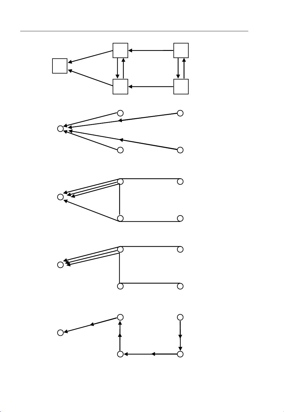
86 Cognitive Radio Networks
1
1
2
12
4
3 5
1
=
D
1
2
1
0
=
D
1
1
=
D
3
2
1
=
D 9
2
8
4
24
2
1
∞=
D
4
1
∞=
D4
5
2
=
D
4
at most 2 arcs
2
0
=
D
1
2
=
D
3
3
1
=
D 9
2
2
=
D2
6
5
3
=
D
4
at most 3 arcs
3
0
=
D
1
3
=
D
3
4
1
=
D 9
2
3
=
D2
4
5
4
=
D
4
Final Tree Of
4
D2
5
Short Paths
4
=
4
0
=
D
1
4
=
D
3
Figure 3.22 Illustration of the Bellman-Ford algorithm
Page 97

Wireless Networks 87
3
2
1
3
2
1
Bellman-Ford
1
Dij Kstra
D
1
D
6
44
2
=
D
2
2
2
4
=
D
1
3
3
4
1
1
=
D
2
2
11
5
1
1
4
1
=
D
4
4
4
=
D
1
=
2
2
3
3
1
4
=
4
5
=
D
4
2
5
4
2
=
D
4
3
=
D
2
2
5
2
2
=
D
4
5
3
3
=
D
1
3
3
6
=
D
6
6
4
3
=
D
3
4
5
3
2
=
D
5
Figure 3.23 Bellman-Ford algorithm and Dijkstra algorithm
3
=
D
2
2
1
4
3
=
D
4
D
1
3
D
4
3
=
D
1
3
3
3
3
=
D
6
6
6
4
5
=
D
5
3
=
D
3
3
1
=
2
2
2
5
3
=
D
3
3
6
3
6
5
=
D
4
=
3
5
3
=
D
5
6
2
Step 2: (Updating of labels) For all j =2P
Dj: ¼ min½Dj; dijþDið3:92Þ
Go to step 1.
We claim that at the beginning of each step 1:
(a) Di Dj, 8i
is, for each node j, the shortest distance from j to 1 using paths with all nodes except possibly
(b) D
j
2
P and j =2P.
j belonging to the set P.
3.4.7.3 Optimal Routing
The monotonically increasing function (cost function) is
X
DijðFijÞ
ði;jÞ
A frequently used formula is
F
D
ijðFij
Þ¼
ij
CijF
þdijF
ij
ij
ð3:93Þ
Page 98

88 Cognitive Radio Networks
where Cijis the transmission capacity of link (i, j) measured in the same unit as Fij. Fijis the total flow
carried by link (i, j)
X
¼
F
ij
x
all path p
containingði; j Þ
p
ð3:94Þ
where x
is the flow of path p. For every origin-destination pair w, there are the constraints
p
X
where r
is the given traffic input of the OD pair and Pwis the set of directed paths of w. In terms of the
w
unknown path flow vector x ¼{x
xp¼ rw; xp 0; 8p 2 P
p2P
w
|p2PW, w2W}, the problem is
p
minimise
X
ði;jÞ
"
D
ij
all paths p
containingði; j Þ
X
w
#
x
p
X
subject to
x
p
We assumethat each D
is a differentiable function of Fijand isdefined in an interval [0,Cij], whereC
ij
is a positive number or infinity. Let x be the vector of path flows x
DðxÞ¼
xp¼ rw; 8w 2 W
p2P
W
0; 8p 2 PW; w 2 W
X
ði;jÞ
D
"
ij
all paths p
containði; j Þ
X
#
x
p
p
Then,
p
X
¼
all linksði; jÞ
on path p
0
D
ij
where the first derivativesD
qDðxÞ
qx
0
are evaluated at the total flows corresponding to x. qD(x)/qxpis the length
ij
of path p when the length of each link (i, j) is taken to be the first derivative D
Consequently, in what follows, qD(x)/qx
*
*
¼fx
Let x
g be an optimal path flow vector. Then, if x
p
must be able to shift a small amount d > 0 from path p to any other path p
improving the cost; otherwise, the optimality would be violated. To get x
is called the first derivative length of path p.
p
*
> 0 for some path p of an OD pair w,we
p
0
of the same OD pair without
*
,
p
0
evaluated at x.
ij
ð3:95Þ
ð3:96Þ
ij
ð3:97Þ
ð3:98Þ
qDðx*Þ
d
qx
qDðx*Þ
0
qx
p
0
p
qDðx*Þ
d
qDðx*Þ
qx
p
0 ð3:99Þ
qx
p
; 8p02 P
W
ð3:100Þ
Optimal path flow is positive only on paths with a minimum first derivative length. Furthermore, at
the optimum, the paths along which the input flow r
less or equal length to that of all other paths of w). If D
of OD pair w is split must have equal length (and
w
is arc convex, the above is a necessary and
ij
sufficient condition for optimality.
Page 99

Wireless Networks 89
In some datagram networks or in networks where detailed path descriptions are not known at the
origin nodes, it may be necessary to maintain, in a routing table at each node i, a routing variable f
(j)
ik
for each link (i, j) and destination j. The routing variable is defined as the fraction of all flow arriving at
node i, destined for node j, and routed along link (i, j):
fikðjÞ
fðk; jÞ¼
P
; 8ði; kÞ; j ð3:101Þ
fimðjÞ
m
where f
solution of the routing problem in terms of the pa th flow variables {x
f
ik
(j) is the flow that travels on link (i, j) and is destined for node j. Given an optimal
ik
*
}, it is possible to determine
p
(j)and fik(j).
3.5 Flow Control
In most networks, there are circumstances in which the externally offered band is larger than can be
handled even with optimal routing. Then, if no measures are taken to restrict the entrance of traffic into
the network, queue sizes at bottleneck links will grow and packet delays will increase similarly to a
motorway traffic jam.
Generally, a need for flow control arises whenever there is a constraint on the communication rate
between two points due to limited capacity of the communication lines or the processing hardware.
Flow control may be required in the transport layer, network layer or Internet layer.
Approaches to flow control include the following:
.
call blocking;
.
packet discarding;
.
packet blocking;
.
packet scheduling.
The main objectives of flow control are to
.
reach a good compromise between throttling sessions (subject to minimum data rate requirements)
and keeping average delay and buffer overflow at a reasonable level;
.
maintain fairness between sessions in providing the requisite quality of service.
3.5.1 Window Flow Control
A session between a transmitter A and a receiver B is said to be window flow controlled if there is an
upper bound on the number of data units that have been transmitted by A and are not yet known by A to
have been received by B. The upper bound (a positive integer) is called the window size.
The receiver B notifies the transmitter A that it has disposed of a data unit by sending a special
message to A, which is called a permit. Upon receiving a permit, A is free to send one more data
unit to B. The general idea in window strategy is that the input rate of the transmitter is reduced
when permits return slowly. Therefore, if there is congestion along the co mmunication path of the
session, the attendant large delays of the permits cause a natural slowdown of the transmitter’s
data rate. However, the window strategy has an additional dimension, whereby the receiver may
intentionally delay permits to restrict the trans mission rate of the session, for example, to avoid
buffer overflow.
The window flow control is typically executed end-to-end. In most common cases, the window size is
aW, where a and W are some positive numbers. Each time a new batch of a data units is received at the
destination node, a permit is sent back to the source allocating a new batch of a data units.
Page 100

d
g
90 Cognitive Radio Networks
Usually, a numbering scheme for packets and permits is used so that permits can be associated
with packets previously transmitted and loss of permits can use a protocol similar to those used for
data link control, whereby a packet contains a sequence number and a request number. Th e latter
number can ser ve as one or more permits for fl ow control purposes. For example, suppose that node
A receives a packet from node B with request number k. Then A knows that B has disposed of all
packets sent by A and numbe red less than k,andAisfreetosendthosepacketsuptonumber
k þ W 1 that it has not sent yet (W is window size). In such a scheme, both the sequenc e number
and the request number are represented modulo m (W þ 1) once packet ordering is preserved
between transmitter and receiver.
It isassumed that thesource node simplycounts the numberx of packets it has already transmitted but
for which it has not yet received back a permit, and transmits new packets only as long as x < W.
Consider the case for a flow of packets where the round-trip delay d including round-trip propagation
delay, packet transmission time and permit delay is smaller than the time required to transmit the full
window of W packets; that is
d WX ð3:102Þ
where X is the transmission time of a single packet. Then the source is capable of transmitting at full
speed of 1/X, and flow control is not active.
For d > WX and the round-trip delay d is so large that full allocation of W packets can be transmitted
before the first permit returns. Assuming that the source always has a packet waiting in queue, the rate of
transmission is W/d.
The maximum rate of transmission corresponding to a round-trip delay d is given by
1
W
r ¼ min
;
x
d
ð3:103Þ
Please also note that the end-to-end windows cannot guarantee a minimum communication rate
(Figure 3.24). In the mean time, we usually need to optimise the window size in wireless networks.
r
Full speed transmission
1
x
Flow control begins
WX
Figure 3.24 End-to-end windows
con
estion
 Loading...