WILEY Coding Theory User Manual

Coding Theory

Coding Theory

Algorithms, Architectures, and

Applications

Andr´e Neubauer

M¨unster University of Applied Sciences, Germany

J¨urgen Freudenberger

HTWG Konstanz, University of Applied Sciences, Germany

Volker K¨uhn

University of Rostock, Germany

Copyright2007JohnWiley&SonsLtd,TheAtrium,SouthernGate,Chichester,

West Sussex PO19 8SQ, England

Telephone [phone]

Email (for orders and customer service enquiries): [e-mail]
Visit our Home Page on www.wileyeurope.com or www.wiley.com

All Rights Reserved. No part of this publication may be reproduced, stored in a retrieval system or transmitted
in any form or by any means, electronic, mechanical, photocopying, recording, scanning or otherwise, except
under the terms of the Copyright, Designs and Patents Act 1988 or under the terms of a licence issued by the
Copyright Licensing Agency Ltd, 90 Tottenham Court Road, London W1T 4LP, UK, without the permission in
writing of the Publisher. Requests to the Publisher should be addressed to the Permissions Department, John
Wiley & Sons Ltd, The Atrium, Southern Gate, Chichester, West Sussex PO19 8SQ, England, or emailed to
[e-mail], or faxed to ([phone].

Designations used by companies to distinguish their products are often claimed as trademarks. All brand names
and product names used in this book are trade names, service marks, trademarks or registered trademarks of
their respective owners. The Publisher is not associated with any product or vendor mentioned in this book. All
trademarks referred to in the text of this publication are the property of their respective owners.

This publication is designed to provide accurate and authoritative information in regard to the subject matter
covered. It is sold on the understanding that the Publisher is not engaged in rendering professional services. If
professional advice or other expert assistance is required, the services of a competent professional should be
sought.

Other Wiley Editorial Offices

John Wiley & Sons Inc., 111 River Street, Hoboken, NJ 07030, USA

Jossey-Bass, 989 Market Street, San Francisco, CA 94103-1741, USA

Wiley-VCH Verlag GmbH, Boschstr. 12, D-69469 Weinheim, Germany

John Wiley & Sons Australia Ltd, 42 McDougall Street, Milton, Queensland 4064, Australia

John Wiley & Sons (Asia) Pte Ltd, 2 Clementi Loop #02-01, Jin Xing Distripark, Singapore 129809

John Wiley & Sons Canada Ltd, 6045 Freemont Blvd, Mississauga, Ontario, L5R 4J3, Canada

Wiley also publishes its books in a variety of electronic formats. Some content that appears
in print may not be available in electronic books.

Anniversary Logo Design: Richard J. Pacifico

Library of Congress Cataloging-in-Publication Data

Neubauer, Andre.

Coding theory : algorithms, architectures and applications / Andre

Neubauer, J¨urgen Freudenberger, Volker K¨uhn.

p. cm.

ISBN 978-0-470-02861-2 (cloth)

1. Coding theory. I Freudenberger, Jrgen. II. K¨uhn, Volker. III.

Title

QA268.N48 2007



003

.54–dc22

British Library Cataloguing in Publication Data

A catalogue record for this book is available from the British Library

ISBN 978-0-470-02861-2 (HB)

Typeset in 10/12pt Times by Laserwords Private Limited, Chennai, India
Printed and bound in Great Britain by Antony Rowe Ltd, Chippenham, Wiltshire
This book is printed on acid-free paper responsibly manufactured from sustainable forestry
in which at least two trees are planted for each one used for paper production.

Contents

Preface ix

1 Introduction 1

1.1 Communication Systems . . . . . . . . . . . . . . . . . . . . . . . . . . . . 1

1.2 Information Theory . . . . . . . . . . . . . . . . . . . . . . . . . . . . . . . 3

1.2.1 Entropy . . . . . . . . . . . . . . . . . . . . . . . . . . . . . . . . . 3

1.2.2 Channel Capacity . . . . . . . . . . . . . . . . . . . . . . . . . . . . 4

1.2.3 Binary Symmetric Channel . . . . . . . . . . . . . . . . . . . . . . 5

1.2.4 AWGN Channel . . . . . . . . . . . . . . . . . . . . . . . . . . . . 6

1.3 A Simple Channel Code . . . . . . . . . . . . . . . . . . . . . . . . . . . . 8

2 Algebraic Coding Theory 13

2.1 Fundamentals of Block Codes . . . . . . . . . . . . . . . . . . . . . . . . . 14

2.1.1 Code Parameters . . . . . . . . . . . . . . . . . . . . . . . . . . . . 16

2.1.2 Maximum Likelihood Decoding . . . . . . . . . . . . . . . . . . . . 19

2.1.3 Binary Symmetric Channel . . . . . . . . . . . . . . . . . . . . . . 23

2.1.4 Error Detection and Error Correction . . . . . . . . . . . . . . . . . 25

2.2 Linear Block Codes . . . . . . . . . . . . . . . . . . . . . . . . . . . . . . . 27

2.2.1 Definition of Linear Block Codes . . . . . . . . . . . . . . . . . . . 27

2.2.2 Generator Matrix . . . . . . . . . . . . . . . . . . . . . . . . . . . . 27

2.2.3 Parity-Check Matrix . . . . . . . . . . . . . . . . . . . . . . . . . . 30

2.2.4 Syndrome and Cosets . . . . . . . . . . . . . . . . . . . . . . . . . 31

2.2.5 Dual Code . . . . . . . . . . . . . . . . . . . . . . . . . . . . . . . 36

2.2.6 Bounds for Linear Block Codes . . . . . . . . . . . . . . . . . . . . 37

2.2.7 Code Constructions . . . . . . . . . . . . . . . . . . . . . . . . . . 41

2.2.8 Examples of Linear Block Codes . . . . . . . . . . . . . . . . . . . 46

2.3 Cyclic Codes . . . . . . . . . . . . . . . . . . . . . . . . . . . . . . . . . . 62

2.3.1 Definition of Cyclic Codes . . . . . . . . . . . . . . . . . . . . . . 62

2.3.2 Generator Polynomial . . . . . . . . . . . . . . . . . . . . . . . . . 63

2.3.3 Parity-Check Polynomial . . . . . . . . . . . . . . . . . . . . . . . . 67

2.3.4 Dual Codes . . . . . . . . . . . . . . . . . . . . . . . . . . . . . . . 70

2.3.5 Linear Feedback Shift Registers . . . . . . . . . . . . . . . . . . . . 71

2.3.6 BCH Codes . . . . . . . . . . . . . . . . . . . . . . . . . . . . . . . 74

2.3.7 Reed–Solomon Codes . . . . . . . . . . . . . . . . . . . . . . . . . 81

vi CONTENTS

2.3.8 Algebraic Decoding Algorithm . . . . . . . . . . . . . . . . . . . . 84

2.4 Summary . . . . . . . . . . . . . . . . . . . . . . . . . . . . . . . . . . . . 93

3 Convolutional Codes 97

3.1 Encoding of Convolutional Codes . . . . . . . . . . . . . . . . . . . . . . . 98

3.1.1 Convolutional Encoder . . . . . . . . . . . . . . . . . . . . . . . . . 98

3.1.2 Generator Matrix in the Time Domain . . . . . . . . . . . . . . . . 101

3.1.3 State Diagram of a Convolutional Encoder . . . . . . . . . . . . . . 103

3.1.4 Code Termination . . . . . . . . . . . . . . . . . . . . . . . . . . . 104

3.1.5 Puncturing . . . . . . . . . . . . . . . . . . . . . . . . . . . . . . . 106

3.1.6 Generator Matrix in the D-Domain . . . . . . . . . . . . . . . . . . 108

3.1.7 Encoder Properties . . . . . . . . . . . . . . . . . . . . . . . . . . . 110

3.2 Trellis Diagram and the Viterbi Algorithm . . . . . . . . . . . . . . . . . . 112

3.2.1 Minimum Distance Decoding . . . . . . . . . . . . . . . . . . . . . 113

3.2.2 Trellises . . . . . . . . . . . . . . . . . . . . . . . . . . . . . . . . . 115

3.2.3 Viterbi Algorithm . . . . . . . . . . . . . . . . . . . . . . . . . . . 116

3.3 Distance Properties and Error Bounds . . . . . . . . . . . . . . . . . . . . . 121

3.3.1 Free Distance . . . . . . . . . . . . . . . . . . . . . . . . . . . . . . 121

3.3.2 Active Distances . . . . . . . . . . . . . . . . . . . . . . . . . . . . 122

3.3.3 Weight Enumerators for Terminated Codes . . . . . . . . . . . . . . 126

3.3.4 Path Enumerators . . . . . . . . . . . . . . . . . . . . . . . . . . . . 129

3.3.5 Pairwise Error Probability . . . . . . . . . . . . . . . . . . . . . . . 131

3.3.6 Viterbi Bound . . . . . . . . . . . . . . . . . . . . . . . . . . . . . 134

3.4 Soft-input Decoding . . . . . . . . . . . . . . . . . . . . . . . . . . . . . . 136

3.4.1 Euclidean Metric . . . . . . . . . . . . . . . . . . . . . . . . . . . . 136

3.4.2 Support of Punctured Codes . . . . . . . . . . . . . . . . . . . . . . 137

3.4.3 Implementation Issues . . . . . . . . . . . . . . . . . . . . . . . . . 138

3.5 Soft-output Decoding . . . . . . . . . . . . . . . . . . . . . . . . . . . . . . 140

3.5.1 Derivation of APP Decoding . . . . . . . . . . . . . . . . . . . . . 141

3.5.2 APP Decoding in the Log Domain . . . . . . . . . . . . . . . . . . 145

3.6 Convolutional Coding in Mobile Communications . . . . . . . . . . . . . . 147

3.6.1 Coding of Speech Data . . . . . . . . . . . . . . . . . . . . . . . . 147

3.6.2 Hybrid ARQ . . . . . . . . . . . . . . . . . . . . . . . . . . . . . . 150

3.6.3 EGPRS Modulation and Coding . . . . . . . . . . . . . . . . . . . . 152

3.6.4 Retransmission Mechanism . . . . . . . . . . . . . . . . . . . . . . 155

3.6.5 Link Adaptation . . . . . . . . . . . . . . . . . . . . . . . . . . . . 156

3.6.6 Incremental Redundancy . . . . . . . . . . . . . . . . . . . . . . . . 157

3.7 Summary . . . . . . . . . . . . . . . . . . . . . . . . . . . . . . . . . . . . 160

4 Turbo Codes 163

4.1 LDPC Codes . . . . . . . . . . . . . . . . . . . . . . . . . . . . . . . . . . 165

4.1.1 Codes Based on Sparse Graphs . . . . . . . . . . . . . . . . . . . . 165

4.1.2 Decoding for the Binary Erasure Channel . . . . . . . . . . . . . . 168

4.1.3 Log-Likelihood Algebra . . . . . . . . . . . . . . . . . . . . . . . . 169

4.1.4 Belief Propagation . . . . . . . . . . . . . . . . . . . . . . . . . . . 174

4.2 A First Encounter with Code Concatenation . . . . . . . . . . . . . . . . . 177

4.2.1 Product Codes . . . . . . . . . . . . . . . . . . . . . . . . . . . . . 177

CONTENTS vii

4.2.2 Iterative Decoding of Product Codes . . . . . . . . . . . . . . . . . 180

4.3 Concatenated Convolutional Codes . . . . . . . . . . . . . . . . . . . . . . 182

4.3.1 Parallel Concatenation . . . . . . . . . . . . . . . . . . . . . . . . . 182

4.3.2 The UMTS Turbo Code . . . . . . . . . . . . . . . . . . . . . . . . 183

4.3.3 Serial Concatenation . . . . . . . . . . . . . . . . . . . . . . . . . . 184

4.3.4 Partial Concatenation . . . . . . . . . . . . . . . . . . . . . . . . . . 185

4.3.5 Turbo Decoding . . . . . . . . . . . . . . . . . . . . . . . . . . . . 186

4.4 EXIT Charts . . . . . . . . . . . . . . . . . . . . . . . . . . . . . . . . . . 188

4.4.1 Calculating an EXIT Chart . . . . . . . . . . . . . . . . . . . . . . 189

4.4.2 Interpretation . . . . . . . . . . . . . . . . . . . . . . . . . . . . . . 191

4.5 Weight Distribution . . . . . . . . . . . . . . . . . . . . . . . . . . . . . . . 196

4.5.1 Partial Weights . . . . . . . . . . . . . . . . . . . . . . . . . . . . . 196

4.5.2 Expected Weight Distribution . . . . . . . . . . . . . . . . . . . . . 197

4.6 Woven Convolutional Codes . . . . . . . . . . . . . . . . . . . . . . . . . . 198

4.6.1 Encoding Schemes . . . . . . . . . . . . . . . . . . . . . . . . . . . 200

4.6.2 Distance Properties of Woven Codes . . . . . . . . . . . . . . . . . 202

4.6.3 Woven Turbo Codes . . . . . . . . . . . . . . . . . . . . . . . . . . 205

4.6.4 Interleaver Design . . . . . . . . . . . . . . . . . . . . . . . . . . . 208

4.7 Summary . . . . . . . . . . . . . . . . . . . . . . . . . . . . . . . . . . . . 212

5 Space–Time Codes 215

5.1 Introduction . . . . . . . . . . . . . . . . . . . . . . . . . . . . . . . . . . . 215

5.1.1 Digital Modulation Schemes . . . . . . . . . . . . . . . . . . . . . . 216

5.1.2 Diversity . . . . . . . . . . . . . . . . . . . . . . . . . . . . . . . . 223

5.2 Spatial Channels . . . . . . . . . . . . . . . . . . . . . . . . . . . . . . . . 229

5.2.1 Basic Description . . . . . . . . . . . . . . . . . . . . . . . . . . . . 229

5.2.2 Spatial Channel Models . . . . . . . . . . . . . . . . . . . . . . . . 234

5.2.3 Channel Estimation . . . . . . . . . . . . . . . . . . . . . . . . . . 239

5.3 Performance Measures . . . . . . . . . . . . . . . . . . . . . . . . . . . . . 241

5.3.1 Channel Capacity . . . . . . . . . . . . . . . . . . . . . . . . . . . . 241

5.3.2 Outage Probability and Outage Capacity . . . . . . . . . . . . . . . 250

5.3.3 Ergodic Error Probability . . . . . . . . . . . . . . . . . . . . . . . 252

5.4 Orthogonal Space – Time Block Codes . . . . . . . . . . . . . . . . . . . . . 257

5.4.1 Alamouti’s Scheme . . . . . . . . . . . . . . . . . . . . . . . . . . . 257

5.4.2 Extension to More than Two Transmit Antennas . . . . . . . . . . . 260

5.4.3 Simulation Results . . . . . . . . . . . . . . . . . . . . . . . . . . . 263

5.5 Spatial Multiplexing . . . . . . . . . . . . . . . . . . . . . . . . . . . . . . 265

5.5.1 General Concept . . . . . . . . . . . . . . . . . . . . . . . . . . . . 265

5.5.2 Iterative APP Preprocessing and Per-layer Decoding . . . . . . . . . 267

5.5.3 Linear Multilayer Detection . . . . . . . . . . . . . . . . . . . . . . 272

5.5.4 Original BLAST Detection . . . . . . . . . . . . . . . . . . . . . . 275

5.5.5 QL Decomposition and Interference Cancellation . . . . . . . . . . 278

5.5.6 Performance of Multi-Layer Detection Schemes . . . . . . . . . . . 287

5.5.7 Unified Description by Linear Dispersion Codes . . . . . . . . . . . 291

5.6 Summary . . . . . . . . . . . . . . . . . . . . . . . . . . . . . . . . . . . . 294

viii CONTENTS

A Algebraic Structures 295

A.1 Groups, Rings and Finite Fields . . . . . . . . . . . . . . . . . . . . . . . . 295

A.1.1 Groups . . . . . . . . . . . . . . . . . . . . . . . . . . . . . . . . . 295

A.1.2 Rings . . . . . . . . . . . . . . . . . . . . . . . . . . . . . . . . . . 296

A.1.3 Finite Fields . . . . . . . . . . . . . . . . . . . . . . . . . . . . . . 298

A.2 Vector Spaces . . . . . . . . . . . . . . . . . . . . . . . . . . . . . . . . . . 299

A.3 Polynomials and Extension Fields . . . . . . . . . . . . . . . . . . . . . . . 300

A.4 Discrete Fourier Transform . . . . . . . . . . . . . . . . . . . . . . . . . . . 305

B Linear Algebra 311

C Acronyms 319

Bibliography 325

Index 335

Preface

Modern information and communication systems are based on the reliable and efficient
transmission of information. Channels encountered in practical applications are usually
disturbed regardless of whether they correspond to information transmission over noisy
and time-variant mobile radio channels or to information transmission on optical discs that
might be damaged by scratches. Owing to these disturbances, appropriate channel coding
schemes have to be employed such that errors within the transmitted information can be
detected or even corrected. To this end, channel coding theory provides suitable coding
schemes for error detection and error correction. Besides good code characteristics with
respect to the number of errors that can be detected or corrected, the complexity of the
architectures used for implementing the encoding and decoding algorithms is important for
practical applications.

The present book provides a concise overview of channel coding theory and practice

as well as the accompanying algorithms, architectures and applications. The selection of
the topics presented in this book is oriented towards those subjects that are relevant for
information and communication systems in use today or in the near future. The focus
is on those aspects of coding theory that are important for the understanding of these
systems. This book places emphasis on the algorithms for encoding and decoding and their
architectures, as well as the applications of the corresponding coding schemes in a unified
framework.

The idea for this book originated from a two-day seminar on coding theory in the

industrial context. We have tried to keep this seminar style in the book by highlighting the
most important facts within the figures and by restricting the scope to the most important
topics with respect to the applications of coding theory, especially within communication
systems. This also means that many important and interesting topics could not be covered
in order to be as concise as possible.

The target audience for the book are students of communication and information engi-

neering as well as computer science at universities and also applied mathematicians who are
interested in a presentation that subsumes theory and practice of coding theory without sac­rificing exactness or relevance with regard to real-world practical applications. Therefore,
this book is well suited for engineers in industry who want to know about the theoretical
basics of coding theory and their application in currently relevant communication systems.

The book is organised as follows. In Chapter 1 a brief overview of the principle

architecture of a communication system is given and the information theory fundamentals
underlying coding theory are summarised. The most important concepts of information the­ory, such as entropy and channel capacity as well as simple channel models, are described.

x PREFACE

Chapter 2 presents the classical, i.e. algebraic, coding theory. The fundamentals of the

encoding and decoding of block codes are explained, and the maximum likelihood decoding
rule is derived as the optimum decoding strategy for minimising the word error probability
after decoding a received word. Linear block codes and their definition based on generator
and parity-check matrices are discussed. General performance measures and bounds relating
important code characteristics such as the minimum Hamming distance and the code rate
are presented, illustrating the compromises necessary between error detection and error
correction capabilities and transmission efficiency. It is explained how new codes can be
constructed from already known codes. Repetition codes, parity-check-codes, Hamming
codes, simplex codes and Reed – Muller codes are presented as examples. Since the task
of decoding linear block codes is difficult in general, the algebraic properties of cyclic
codes are exploited for efficient decoding algorithms. These cyclic codes, together with
their generator and parity-check polynomials, are discussed, as well as efficient encoding
and decoding architectures based on linear feedback shift registers. Important cyclic codes
such as BCH codes and Reed – Solomon codes are presented, and an efficient algebraic
decoding algorithm for the decoding of these cyclic codes is derived.

Chapter 3 deals with the fundamentals of convolutional coding. Convolutional codes

can be found in many applications, for instance in dial-up modems, satellite communications
and digital cellular systems. The major reason for this popularity is the existence of efficient
decoding algorithms that can utilise soft input values from the demodulator. This so-called
soft-input decoding leads to significant performance gains. Two famous examples for a
soft-input decoding algorithm are the Viterbi algorithm and the Bahl, Cocke, Jelinek, Raviv
(BCJR) algorithm which also provides a reliability output. Both algorithms are based on
the trellis representation of the convolutional code. This highly repetitive structure makes
trellis-based decoding very suitable for hardware implementations.

We start our discussion with the encoding of convolutional codes and some of their

basic properties. It follows a presentation of the Viterbi algorithm and an analysis of
the error correction performance with this maximum likelihood decoding procedure. The
concept of soft-output decoding and the BCJR algorithm are considered in Section 3.5. Soft­output decoding is a prerequisite for the iterative decoding of concatenated convolutional
codes as introduced in Chapter 4. Finally, we consider an application of convolutional
codes for mobile communication channels as defined in the Global System for Mobile
communications (GSM) standard. In particular, the considered hybrid ARQ protocols are
excellent examples of the adaptive coding systems that are required for strongly time-variant
mobile channels.

As mentioned above, Chapter 4 is dedicated to the construction of long powerful codes

based on the concatenation of simple convolutional component codes. These concatenated
convolutional codes, for example the famous turbo codes, are capable of achieving low
bit error rates at signal-to-noise ratios close to the theoretical Shannon limit. The term
turbo reflects a property of the employed iterative decoding algorithm, where the decoder
output of one iteration is used as the decoder input of the next iteration. This concept
of iterative decoding was first introduced for the class of low-density parity-check codes.
Therefore, we first introduce low-density parity-check codes in Section 4.1 and discuss
the relation between these codes and concatenated code constructions. Then, we introduce
some popular encoding schemes for concatenated convolutional codes and present three
methods to analyse the performance of the corresponding codes. The EXIT chart method

PREFACE xi

in Section 4.4 makes it possible to predict the behaviour of the iterative decoder by looking
at the input/output relations of the individual constituent soft-output decoders. Next, we
present a common approach in coding theory. We estimate the code performance with
maximum likelihood decoding for an ensemble of concatenated codes. This method explains
why many concatenated code constructions lead to a low minimum Hamming distance and
therefore to a relatively poor performance for high signal-to-noise ratios. In Section 4.6 we
consider code designs that lead to a higher minimum Hamming distance owing to a special
encoder construction, called the woven encoder, or the application of designed interleavers.

The fifth chapter addresses space – time coding concepts, a still rather new topic in the

area of radio communications. Although these techniques do not represent error-correcting
codes in the classical sense, they can also be used to improve the reliability of a data
link. Since space –time coding became popular only a decade ago, only a few concepts
have found their way into current standards hitherto. However, many other approaches are
currently being discussed. As already mentioned before, we restrict this book to the most
important and promising concepts.

While classical encoders and decoders are separated from the physical channel by

modulators, equalisers, etc., and experience rather simple hyperchannels, this is not true
for space–time coding schemes. They directly work on the physical channel. Therefore,
Chapter 5 starts with a short survey of linear modulation schemes and explains the prin­ciple of diversity. Next, spatial channel models are described and different performance
measures for their quantitative evaluation are discussed. Sections 5.4 and 5.5 introduce
two space – time coding concepts with the highest practical relevance, namely orthogonal
space–time block codes increasing the diversity degree and spatial multiplexing techniques
boosting the achievable data rate. For the latter approach, sophisticated signal processing
algorithms are required at the receiver in order to separate superimposed data streams again.

In the appendices a brief summary of algebraic structures such as finite fields and poly-

nomial rings is given, which are needed for the treatment especially of classical algebraic
codes, and the basics of linear algebra are briefly reviewed.

Finally, we would like to thank the Wiley team, especially Sarah Hinton as the respon-

sible editor, for their support during the completion of the manuscript. We also thank
Dr. rer. nat. Jens Schlembach who was involved from the beginning of this book project
and who gave encouragement when needed. Last but not least, we would like to give spe­cial thanks to our families – Fabian, Heike, Jana and Erik, Claudia, Hannah and Jakob and
Christiane – for their emotional support during the writing of the manuscript.

Andr´e Neubauer

M¨unster University of Applied Sciences

J¨urgen Freudenberger

HTWG Konstanz University of Applied Sciences

Volker K¨uhn

University of Rostock

1

Introduction

The reliable transmission of information over noisy channels is one of the basic require­ments of digital information and communication systems. Here, transmission is understood
both as transmission in space, e.g. over mobile radio channels, and as transmission in time
by storing information in appropriate storage media. Because of this requirement, modern
communication systems rely heavily on powerful channel coding methodologies. For practi­cal applications these coding schemes do not only need to have good coding characteristics
with respect to the capability of detecting or correcting errors introduced on the channel.
They also have to be efficiently implementable, e.g. in digital hardware within integrated
circuits. Practical applications of channel codes include space and satellite communica­tions, data transmission, digital audio and video broadcasting and mobile communications,
as well as storage systems such as computer memories or the compact disc (Costello et al.,

1998).
In this introductory chapter we will give a brief introduction into the field of channel

coding. To this end, we will describe the information theory fundamentals of channel
coding. Simple channel models will be presented that will be used throughout the text.
Furthermore, we will present the binary triple repetition code as an illustrative example of
a simple channel code.

1.1 Communication Systems

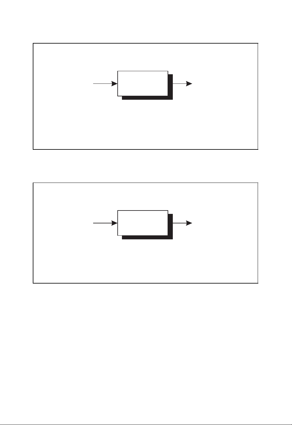
In Figure 1.1 the basic structure of a digital communication system is shown which repre­sents the architecture of the communication systems in use today. Within the transmitter
of such a communication system the following tasks are carried out:

● source encoding,

● channel encoding,

● modulation.

Coding Theory – Algorithms, Architectures, and Applications Andr´e Neubauer, J¨urgen Freudenberger, Volker K¨uhn

 2007 John Wiley & Sons, Ltd

2 INTRODUCTION

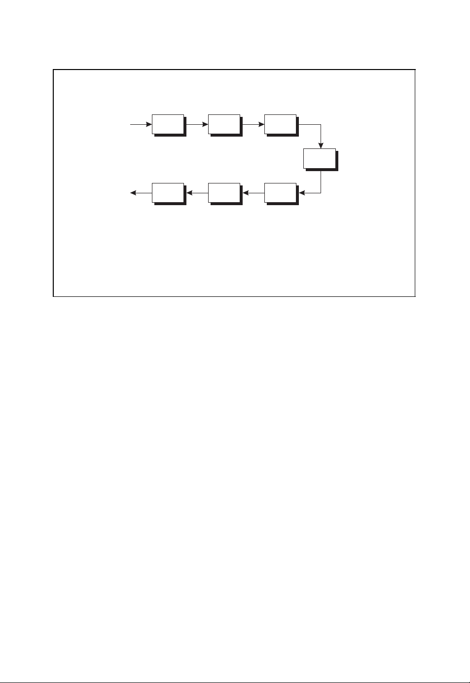
Principal structure of digital communication systems

u

u

ˆ

channel

FEC

encoder

encoder

channel

FEC

decoder

encoder

source

source

FEC

encoder

encoder

encoder

source

FEC

decoder

encoder

■ The sequence of information symbols u is encoded into the sequence of

b

modu-

FEC

lator

encoder

FEC

channel

encoder

r

demo-

FEC

dulator

encoder

code symbols b which are transmitted across the channel after modulation.

■ The sequence of received symbols r is decoded into the sequence of

information symbolsˆu which are estimates of the originally transmitted
information symbols.

Figure 1.1: Basic structure of digital communication systems

In the receiver the corresponding inverse operations are implemented:

● demodulation,

● channel decoding,

● source decoding.

According to Figure 1.1 the modulator generates the signal that is used to transmit the
sequence of symbols b across the channel (Benedetto and Biglieri, 1999; Neubauer, 2007;
Proakis, 2001). Due to the noisy nature of the channel, the transmitted signal is disturbed.
The noisy received signal is demodulated by the demodulator in the receiver, leading to the
sequence of received symbols r. Since the received symbol sequence r usually differs from
the transmitted symbol sequence b,achannel code is used such that the receiver is able to
detect or even correct errors (Bossert, 1999; Lin and Costello, 2004; Neubauer, 2006b). To
this end, the channel encoder introduces redundancy into the information sequence u. This
redundancy can be exploited by the channel decoder for error detection or error correction
by estimating the transmitted symbol sequenceˆu.

In his fundamental work, Shannon showed that it is theoretically possible to realise an

information transmission system with as small an error probability as required (Shannon,

1948). The prerequisite for this is that the information rate of the information source

be smaller than the so-called channel capacity. In order to reduce the information rate,
source coding schemes are used which are implemented by the source encoder in the
transmitter and the source decoder in the receiver (McEliece, 2002; Neubauer, 2006a).

INTRODUCTION 3

Further information about source coding can be found elsewhere (Gibson et al., 1998;
Sayood, 2000, 2003).

In order better to understand the theoretical basics of information transmission as well

as channel coding, we now give a brief overview of information theory as introduced by
Shannon in his seminal paper (Shannon, 1948). In this context we will also introduce the
simple channel models that will be used throughout the text.

1.2 Information Theory

An important result of information theory is the finding that error-free transmission across a
noisy channel is theoretically possible – as long as the information rate does not exceed the
so-called channel capacity. In order to quantify this result, we need to measure information.
Within Shannon’s information theory this is done by considering the statistics of symbols
emitted by information sources.

1.2.1 Entropy

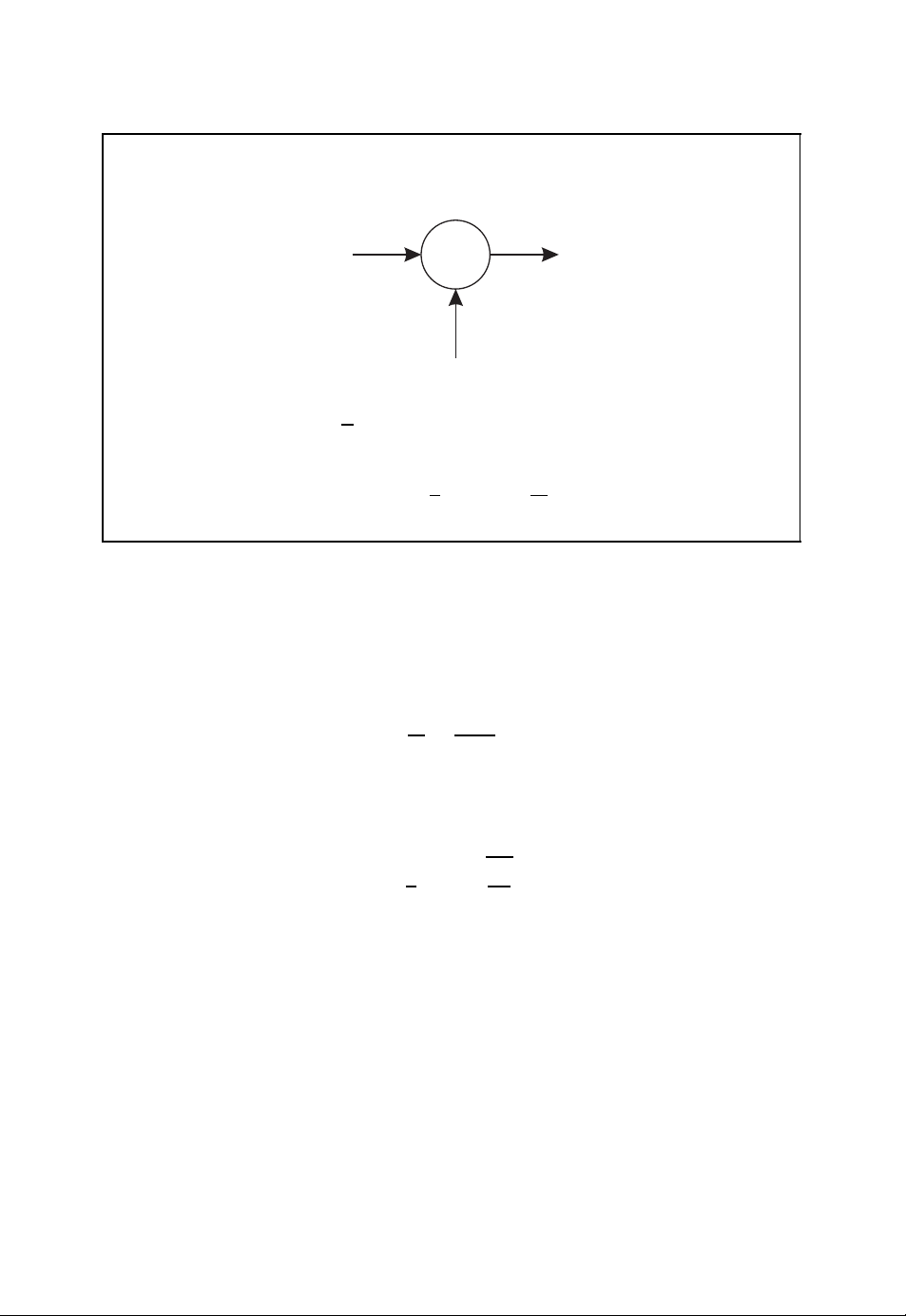
Let us consider the discrete memoryless information source shown in Figure 1.2. At a given
time instant, this discrete information source emits the random discrete symbol X = x
which assumes one out of M possible symbol values x1, x2, ..., xM. The rate at which these
symbol values appear are given by the probabilities P

(xi) = Pr{X = xi}.

P

X

(x1), PX(x2), ..., PX(xM) with

X

i

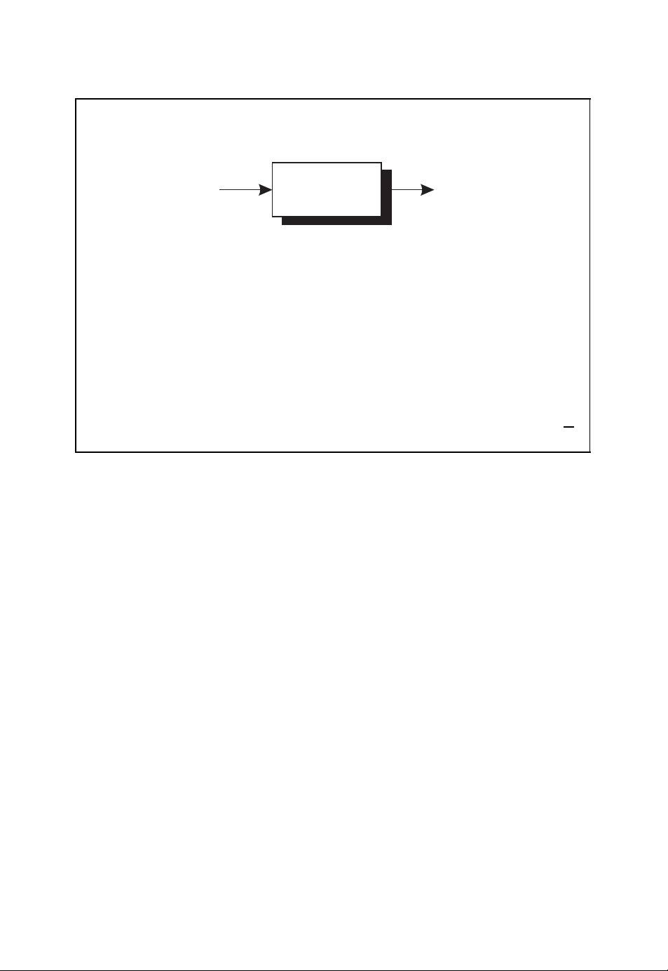
Discrete information source

Information

X

source

■ The discrete information source emits the random discrete symbol X .

■ The symbol values x

..., P

■ Entropy

(xM).

X

Figure 1.2: Discrete information source emitting discrete symbols X

, x2, ..., xMappear with probabilities PX(x1), PX(x2),

1

M



I(X ) =−

PX(xi) · log2(PX(xi)) (1.1)

i=1

4 INTRODUCTION

The average information associated with the random discrete symbol X is given by the
so-called entropy measured in the unit ‘bit’

M

I(X ) =−



PX(xi) · log

i=1

(xi)).

P

(

X

2

For a binary information source that emits the binary symbols X = 0 and X = 1 with
probabilities Pr{X = 0}=p

and Pr{X = 1}=1 −Pr{X = 0}=1 − p0, the entropy is

0

given by the so-called Shannon function or binary entropy function

I(X ) =−p

log2(p0) − (1 −p0) log2(1 −p0).

0

1.2.2 Channel Capacity

With the help of the entropy concept we can model a channel according to Berger’s channel
diagram shown in Figure 1.3 (Neubauer, 2006a). Here, X refers to the input symbol and
R denotes the output symbol or received symbol. We now assume that M input symbol
values x
help of the conditional probabilities

and

the conditional entropies are given by

and

With these conditional probabilities the mutual information

can be derived which measures the amount of information that is transmitted across the
channel from the input to the output for a given information source.

I(X ;R) with respect to the statistical properties of the input X , i.e. by appropriately
choosing the probabilities {P

If the input entropy I(X ) is smaller than the channel capacity C

, x2, ..., xMand N output symbol values r1, r2, ..., rNare possible. With the

1

(xi|rj) = Pr{X = xi|R = rj}

P

X |R

P

(rj|xi) = Pr{R = rj|X = xi}

R|X

M

N



I(X |R) =−

I(R|X ) =−

i=1

M



i=1



j=1

N



j=1

P

(xi,rj) · log

X ,R

P

(xi,rj) · log2(P

X ,R



P

X |R

2

R|X



(xi|rj)

(rj|xi)).

I(X ;R) = I(X ) − I(X |R) = I(R) − I(R|X )

The so-called channel capacity C is obtained by maximising the mutual information

(xi)}

X

C = max

. This leads to

1≤i≤M

{PX(xi)}

I(X )

1≤i≤M

!

<C,

I(X ;R).

then information can be transmitted across the noisy channel with arbitrarily small error
probability. Thus, the channel capacity C in fact quantifies the information transmission
capacity of the channel.

INTRODUCTION 5

Berger’s channel diagram

I(X |R)

I(X )

I(X ;R)

I(R)

I(R|X )

■ Mutual information

I(X ;R) = I(X ) − I(X |R) = I(R) − I(R|X ) (1.2)

■ Channel capacity

C = max

{PX(xi)}

I(X ;R) (1.3)

1≤i≤M

Figure 1.3: Berger’s channel diagram

1.2.3 Binary Symmetric Channel

As an important example of a memoryless channel we turn to the binary symmetric channel
or BSC. Figure 1.4 shows the channel diagram of the binary symmetric channel with bit
error probability ε. This channel transmits the binary symbol X = 0orX = 1 correctly
with probability 1 −ε, whereas the incorrect binary symbol R = 1orR = 0 is emitted
with probability ε.

By maximising the mutual information I(X ;R), the channel capacity of a binary

symmetric channel is obtained according to

C = 1 + ε log

This channel capacity is equal to 1 if ε = 0orε = 1; for ε =

(ε) + (1 − ε) log2(1 −ε).

2

1
2

the channel capacity is 0. In
contrast to the binary symmetric channel, which has discrete input and output symbols taken
from binary alphabets, the so-called AWGN channel is defined on the basis of continuous
real-valued random variables.

1

In Chapter 5 we will also consider complex-valued random variables.

1

6 INTRODUCTION

Binary symmetric channel

1 −ε

X = 0

ε

ε

X = 1

1 −ε

■ Bit error probability ε

■ Channel capacity

R = 0

R = 1

C = 1 + ε log

(ε) + (1 − ε) log2(1 −ε) (1.4)

2

Figure 1.4: Binary symmetric channel with bit error probability ε

1.2.4 AWGN Channel

Up to now we have exclusively considered discrete-valued symbols. The concept of entropy
can be transferred to continuous real-valued random variables by introducing the so-called
differential entropy. It turns out that a channel with real-valued input and output symbols can
again be characterised with the help of the mutual information I(X ;R) and its maximum,
the channel capacity C. In Figure 1.5 the so-called AWGN channel is illustrated which is
described by the additive white Gaussian noise term Z .

With the help of the signal power



S = EX

and the noise power

N = EZ

the channel capacity of the AWGN channel is given by

1

C =

log

2

2



2



2

1 +



S

.

N

The channel capacity exclusively depends on the signal-to-noise ratio S/N.

In order to compare the channel capacities of the binary symmetric channel and the
AWGN channel, we assume a digital transmission scheme using binary phase shift keying
(BPSK) and optimal reception with the help of a matched filter (Benedetto and Biglieri,
1999; Neubauer, 2007; Proakis, 2001). The signal-to-noise ratio of the real-valued output

INTRODUCTION 7

AWGN channel

X

+

R

Z

■ Signal-to-noise ratio

■ Channel capacity

S

N

C =



1

log

2

2

1 +



S

N

(1.5)

Figure 1.5: AWGN channel with signal-to-noise ratio S/N

R of the matched filter is then given by

S

E

b

=

N

N0/2

with bit energy E

and noise power spectral density N0. If the output R of the matched

b

filter is compared with the threshold 0, we obtain the binary symmetric channel with bit
error probability







ε =

1

erfc

2

E

b

.

N

0

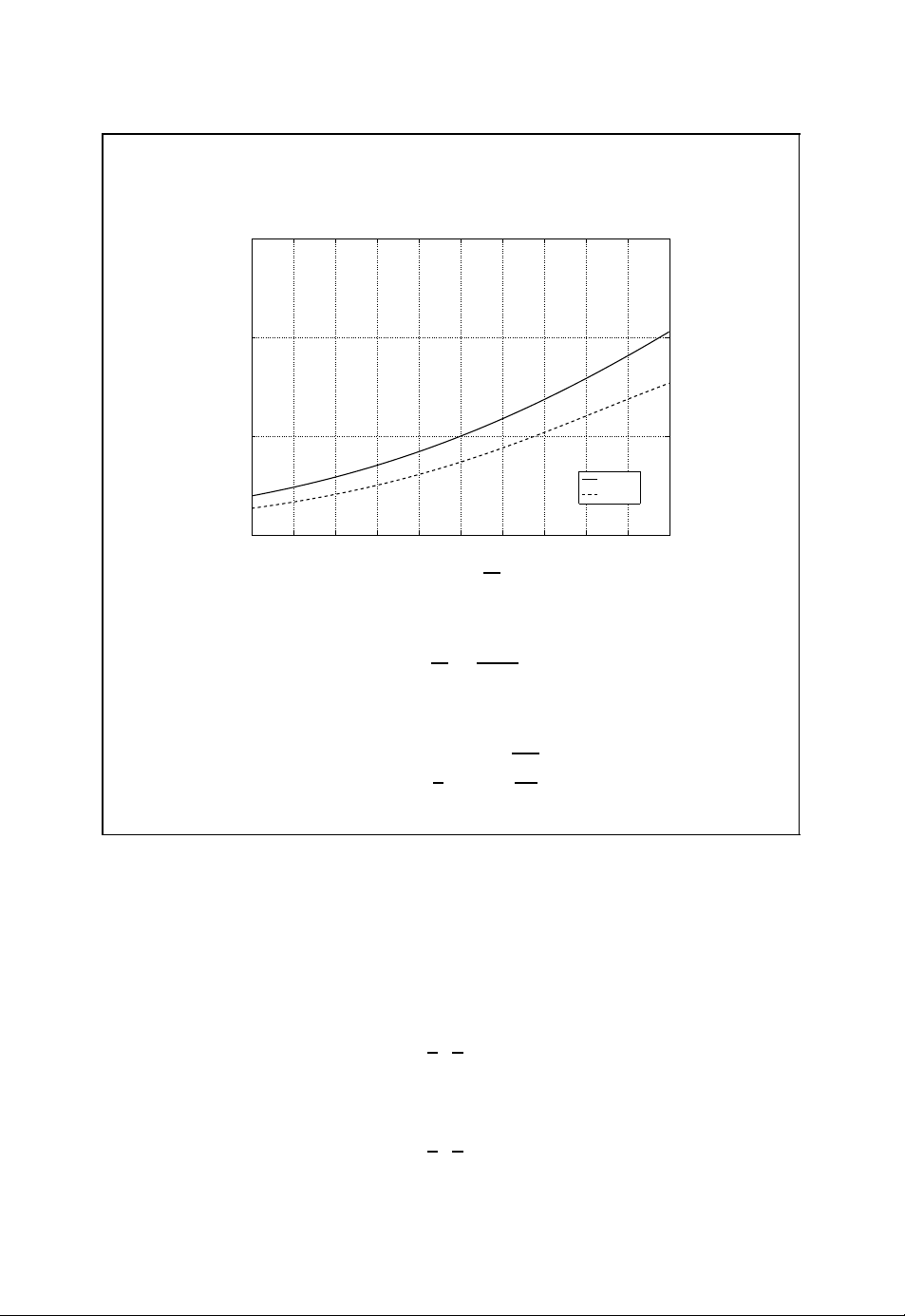
Here, erfc(·) denotes the complementary error function. In Figure 1.6 the channel capaci­ties of the binary symmetric channel and the AWGN channel are compared as a function
of E

. The signal-to-noise ratio S/N or the ratio Eb/N0must be higher for the binary

b/N0

symmetric channel compared with the AWGN channel in order to achieve the same channel
capacity. This gain also translates to the coding gain achievable by soft-decision decoding
as opposed to hard-decision decoding of channel codes, as we will see later (e.g. in
Section 2.2.8).

Although information theory tells us that it is theoretically possible to find a channel
code that for a given channel leads to as small an error probability as required, the design
of good channel codes is generally difficult. Therefore, in the next chapters several classes
of channel codes will be described. Here, we start with a simple example.

8 INTRODUCTION

Channel capacity of BSC vs AWGN channel

1.5

1

C

0.5

AWGN
BSC

0

Ŧ5 Ŧ4 Ŧ3 Ŧ2 Ŧ1 0 1 2 3 4 5

10 log

■ Signal-to-noise ratio of AWGN channel





E

b

10

N

0

E

S

N

=

b

N0/2

(1.6)

■ Bit error probability of binary symmetric channel







ε =

1

erfc

2

E

b

N

0

(1.7)

Figure 1.6: Channel capacity of the binary symmetric channel vs the channel capacity of

the AWGN channel

1.3 A Simple Channel Code

As an introductory example of a simple channel code we consider the transmission of the
binary information sequence

01110

001

over a binary symmetric channel with bit error probability ε = 0.25 (Neubauer, 2006b).
On average, every fourth binary symbol will be received incorrectly. In this example we
assume that the binary sequence

00110

000

is received at the output of the binary symmetric channel (see Figure 1.7).

INTRODUCTION 9

Channel transmission

00101110

■ Binary symmetric channel with bit error probability ε = 0.25

■ Transmission w/o channel code

BSC

00000110

Figure 1.7: Channel transmission without channel code

Encoder

00101110

■ Binary information symbols 0 and 1

■ Binary code words 000 and 111

■ Binary triple repetition code {000, 111}

Encoder

000000111000111111111000

Figure 1.8: Encoder of a triple repetition code

In order to implement a simple error correction scheme we make use of the so-called
binary triple repetition code. This simple channel code is used for the encoding of binary
data. If the binary symbol 0 is to be transmitted, the encoder emits the code word 000.
Alternatively, the code word 111 is issued by the encoder when the binary symbol 1 is to
be transmitted. The encoder of a triple repetition code is illustrated in Figure 1.8.

For the binary information sequence given above we obtain the binary code sequence

000 000 111 000 111111 111 000

at the output of the encoder. If we again assume that on average every fourth binary
symbol is incorrectly transmitted by the binary symmetric channel, we may obtain the
received sequence

0 000 011 010 111010 111 010.

01

This is illustrated in Figure 1.9.

10 INTRODUCTION

Channel transmission

000000111000111111111000

■ Binary symmetric channel with bit error probability ε = 0.25

■ Transmission with binary triple repetition code

BSC

010000011010111010111010

Figure 1.9: Channel transmission of a binary triple repetition code

Decoder

010000011010111010111010

■ Decoding of triple repetition code by majority decision

Decoder

000 → 000

001 → 000

010 → 000

00101010

011 → 111

.
.
.

110 → 111

111 → 111

Figure 1.10: Decoder of a triple repetition code

The decoder in Figure 1.10 tries to estimate the original information sequence with the
help of a majority decision. If the number of 0s within a received 3-bit word is larger than
the number of 1s, the decoder emits the binary symbol 0; otherwise a 1 is decoded. With
this decoding algorithm we obtain the decoded information sequence

001010

10.

INTRODUCTION 11

As can be seen from this example, the binary triple repetition code is able to correct a single
error within a code word. More errors cannot be corrected. With the help of this simple
channel code we are able to reduce the number of errors. Compared with the unprotected
transmission without a channel code, the number of errors has been reduced from two to
one. However, this is achieved by a significant reduction in the transmission bandwidth
because, for a given symbol rate on the channel, it takes 3 times longer to transmit an
information symbol with the help of the triple repetition code. It is one of the main topics
of the following chapters to present more efficient coding schemes.

2

Algebraic Coding Theory

In this chapter we will introduce the basic concepts of algebraic coding theory. To this end,
the fundamental properties of block codes are first discussed. We will define important code
parameters and describe how these codes can be used for the purpose of error detection
and error correction. The optimal maximum likelihood decoding strategy will be derived
and applied to the binary symmetric channel.

With these fundamentals at hand we will then introduce linear block codes. These
channel codes can be generated with the help of so-called generator matrices owing to
their special algebraic properties. Based on the closely related parity-check matrix and the
syndrome, the decoding of linear block codes can be carried out. We will also introduce
dual codes and several techniques for the construction of new block codes based on known
ones, as well as bounds for the respective code parameters and the accompanying code
characteristics. As examples of linear block codes we will treat the repetition code, parity­check code, Hamming code, simplex code and Reed –Muller code.

Although code generation can be carried out efficiently for linear block codes, the
decoding problem for general linear block codes is difficult to solve. By introducing further
algebraic structures, cyclic codes can be derived as a subclass of linear block codes for
which efficient algebraic decoding algorithms exist. Similar to general linear block codes,
which are defined using the generator matrix or the parity-check matrix, cyclic codes
are defined with the help of the so-called generator polynomial or parity-check polynomial.
Based on linear feedback shift registers, the respective encoding and decoding architectures
for cyclic codes can be efficiently implemented. As important examples of cyclic codes
we will discuss BCH codes and Reed – Solomon codes. Furthermore, an algebraic decoding
algorithm is presented that can be used for the decoding of BCH and Reed–Solomon
codes.

In this chapter the classical algebraic coding theory is presented. In particular, we
will follow work (Berlekamp, 1984; Bossert, 1999; Hamming, 1986; Jungnickel, 1995;
Lin and Costello, 2004; Ling and Xing, 2004; MacWilliams and Sloane, 1998; McEliece,
2002; Neubauer, 2006b; van Lint, 1999) that contains further details about algebraic coding
theory.

Coding Theory – Algorithms, Architectures, and Applications Andr´e Neubauer, J¨urgen Freudenberger, Volker K¨uhn

 2007 John Wiley & Sons, Ltd

14 ALGEBRAIC CODING THEORY

2.1 Fundamentals of Block Codes

In Section 1.3, the binary triple repetition code was given as an introductory example of a
simple channel code. This specific channel code consists of two code words 000 and 111 of
length n = 3, which represent k = 1 binary information symbol 0 or 1 respectively. Each
symbol of a binary information sequence is encoded separately. The respective code word
of length 3 is then transmitted across the channel. The potentially erroneously received word
is finally decoded into a valid code word 000 or 111 – or equivalently into the respective
information symbol 0 or 1. As we have seen, this simple code is merely able to correct
one error by transmitting three code symbols instead of just one information symbol across
the channel.

In order to generalise this simple channel coding scheme and to come up with more effi­cient and powerful channel codes, we now consider an information sequence u
u5u6u7... of discrete information symbols ui. This information sequence is grouped into
blocks of length k according to

u

···u

0u1

  

k−1

block

u

  

kuk+1

···u

block

u

2k−1

2ku2k+1

  

block

···u

3k−1

···.

In so-called q-nary (n, k) block codes the information words

u

0u1

u

kuk+1

u

2ku2k+1

.
.
.

···u

k−1

···u

···u

,

2k−1

3k−1

,

,

0u1u2u3u4

of length k with u

∈{0, 1,...,q−1} are encoded separately from each other into the

i

corresponding code words

b

of length n with b

···b

0b1

b

nbn+1

b

2nb2n+1

.
.
.

∈{0, 1,...,q−1} (see Figure 2.1).1These code words are trans-

i

n−1

···b

···b

,

2n−1

3n−1

,

,

mitted across the channel and the received words are appropriately decoded, as shown
in Figure 2.2. In the following, we will write the information word u
the code word b

0b1

···b

respectively. Accordingly, the received word is denoted by r = (r

1

For q = 2 we obtain the important class of binary channel codes.

as vectors u = (u0,u1,...,u

n−1

) and b = (b0,b1,...,b

k−1

,...,r

0,r1

0u1

···u

n−1

and

k−1

n−1

), whereas

)

ALGEBRAIC CODING THEORY 15

Encoding of an (n, k) block code

(u0,u1,...,u

■ The sequence of information symbols is grouped into words (or blocks) of

k−1

)

Encoder

(b

0,b1

,...,b

equal length k which are independently encoded.

■ Each information word (u

onto a code word (b

0,b1

0,u1

,...,b

,...,u

k−1

) of length n.

n−1

) of length k is uniquely mapped

Figure 2.1: Encoding of an (n, k) block code

Decoding of an (n, k) block code

(r0,r1,...,r

■ The received word (r

decoded into the code word (ˆb
wordˆu = ( ˆu

n−1

)

, ˆu1,..., ˆu

0

Decoder

,...,r

0,r1

) of length k respectively.

k−1

) of length n at the output of the channel is

n−1

,ˆb1,...,ˆb

0

,ˆb1,...,ˆb

(ˆb

0

) of length n or the information

n−1

n−1

n−1

)

)

Figure 2.2: Decoding of an (n, k) block code

the decoded code word and decoded information word are given byˆb = (ˆb
andˆu = ( ˆu

, ˆu1,..., ˆu

0

) respectively. In general, we obtain the transmission scheme for

k−1

,ˆb1,...,ˆb

0

n−1

an (n, k) block code as shown in Figure 2.3.

Without further algebraic properties of the (n, k) block code, the encoding can be carried
out by a table look-up procedure. The information word u to be encoded is used to address
a table that for each information word u contains the corresponding code word b at the
respective address. If each information symbol can assume one out of q possible values,

)

16 ALGEBRAIC CODING THEORY

Encoding, transmission and decoding of an (n, k) block code

■ Information word u = (u

■ Code word b = (b

■ Received word r = (r

■ Decoded code word

■ Decoded information word

u

■ The information word u is encoded into the code word b.

■ The code word b is transmitted across the channel which emits the received

Encoder Channel Decoder

0,b1

0,r1

ˆ

b = (ˆb0,ˆb1,...,ˆb

,...,u

0,u1

,...,b

) of length n

n−1

,...,r

n−1

ˆ

u = ( ˆu0, ˆu1,..., ˆu

b

) of length k

k−1

) of length n

) of length n

n−1

k−1

) of length k

r

word r.

■ Based on the received word r,thecodeword

ˆ

b (or equivalently the

information wordˆu) is decoded.

Figure 2.3: Encoding, transmission and decoding of an (n, k) block code

ˆ

b

k

the number of code words is given by q
total size of the table is nq

k

. The size of the table grows exponentially with increasing

. Since each entry carries nq-nary symbols, the

information word length k. For codes with a large number of code words – corresponding to
a large information word length k – a coding scheme based on a table look-up procedure
is inefficient owing to the large memory size needed. For that reason, further algebraic
properties are introduced in order to allow for a more efficient encoder architecture of an
(n, k) block code. This is the idea lying behind the so-called linear block codes, which we
will encounter in Section 2.2.

2.1.1 Code Parameters

Channel codes are characterised by so-called code parameters. The most important code
parameters of a general (n, k) block code that are introduced in the following are the code
rate and the minimum Hamming distance (Bossert, 1999; Lin and Costello, 2004; Ling and
Xing, 2004). With the help of these code parameters, the efficiency of the encoding process
and the error detection and error correction capabilities can be evaluated for a given (n, k)
block code.

ALGEBRAIC CODING THEORY 17

Code Rate

Under the assumption that each information symbol u
q values, the number of possible information words and code words is given by

of the (n, k) block code can assume

i

2

M = qk.

Since the code word length n is larger than the information word length k, the rate at which
information is transmitted across the channel is reduced by the so-called code rate

(M)

log

R =

For the simple binary triple repetition code with k = 1 and n = 3, the code rate is R =

k

1

=

≈ 0,3333.

n

3

q

n

k

=

.

n

Weight and Hamming Distance

Each code word b = (b
as the number of non-zero components b

0,b1

,...,b

) can be assigned the weight wt(b) which is defined

n−1

= 0 (Bossert, 1999), i.e.

i

3

wt(b) =|{i : bi= 0, 0 ≤ i<n}|.

Accordingly, the distance between two code words b = (b



b

1

The Hamming distance dist(b, b



b
consisting of M code words b



,...,b

) is given by the so-called Hamming distance (Bossert, 1999)

n−1





dist(b, b





i : b

) =



) provides the number of different components of b and

i

= b



, 0 ≤ i<n

i

and thus measures how close the code words b and bare to each other. For a code B

, b2, ..., bM, the minimum Hamming distance is given by

1

0,b1



,...,b





.

) and b= (b

n−1



,

0

d = min

We will denote the (n, k) block code B =

∀b=b

{

b

dist(b, b).



, b2,...,b

1

}

with M = q

M

k

q-nary code words

of length n and minimum Hamming distance d by B(n,k,d). The minimum weight of the
block code B is defined as min

wt(b). The code parameters of B(n,k,d) are summarised

∀b=0

in Figure 2.4.

Weight Distribution

The so-called weight distribution W(x) of an (n, k) block code B ={b

, b2,...,b

1

M

describes how many code words exist with a specific weight. Denoting the number of
code words with weight i by

w

=|{b ∈ B :wt(b) = i

i

2

In view of the linear block codes introduced in the following, we assume here that all possible information
words u = (u

3

|B| denotes the cardinality of the set B.

0,u1

,...,u

) are encoded.

k−1

}|

}

18 ALGEBRAIC CODING THEORY

Code parameters of (n, k) block codes B(n, k, d)

■ Code rate

■ Minimum weight

■ Minimum Hamming distance

d = min

∀b=b

k

R =

n

wt(b) (2.2)

min

∀b=0

dist(b, b) (2.3)



(2.1)

Figure 2.4: Code parameters of (n, k) block codes B(n,k,d)

with 0 ≤ i ≤ n and 0 ≤ w
(Bossert, 1999)

≤ M , the weight distribution is defined by the polynomial

i

n



W(x)=

wixi.

i=0

The minimum weight of the block code B can then be obtained from the weight distribution
according to

wt(b) = min

min

∀b=0

i>0

wi.

Code Space

A q-nary block code B(n,k,d) with code word length n can be illustrated as a subset of
the so-called code space F

q-nary words or vectors.

n

. Such a code space is a graphical illustration of all possible

q

4

The total number of vectors of length n with weight w and

q-nary components is given by





n

w

with the binomial coefficients

The total number of vectors within F

|F

4

In Section 2.2 we will identify the code space with the finite vector space F
algebraic structures such as finite fields and vector spaces the reader is referred to Appendix A.

(q −1)



n

w

n

|=

q

w

=



=

n

is then obtained from

q



n



w=0

n!

w! (n −w)!

n!

w! (n −w)!



n

(q −1)

w

(q −1)

.

w

= qn.

w

n

. For a brief overview of

q

ALGEBRAIC CODING THEORY 19

Four-dimensional binary code space F
































































0000












1111


















































































































4
0



































































0100





1001







1101










































4
1

1000











4
2

1100





4
3





4
4

■ The four-dimensional binary code space F





















1010

1110

vectors of length 4.

4
2



















0010





0110





1011







4
2











0001
















































0101




0111

























consists of 24= 16 binary

0011

wt = 0

wt = 1

wt = 2

wt = 3

wt = 4

Figure 2.5: Four-dimensional binary code space F

4

. Reproduced by permission of

2

J. Schlembach Fachverlag

The four-dimensional binary code space F

4

with q = 2 and n = 4 is illustrated in Figure 2.5

2

(Neubauer, 2006b).

2.1.2 Maximum Likelihood Decoding

Channel codes are used in order to decrease the probability of incorrectly received code
words or symbols. In this section we will derive a widely used decoding strategy. To this
end, we will consider a decoding strategy to be optimal if the corresponding word error

probability

= Pr{ˆu = u}=Pr{ˆb = b}

p

err

is minimal (Bossert, 1999). The word error probability has to be distinguished from the

symbol error probability

k−1



sym

1

=

k

i=0

Pr{ˆui= ui}

p

20 ALGEBRAIC CODING THEORY

Optimal decoder

r

■ The received word r is decoded into the code word

Decoder

ˆ

b(r)

ˆ

b(r) such that the word

error probability

= Pr{ˆu = u}=Pr{ˆb = b} (2.4)

p

err

is minimal.

Figure 2.6: Optimal decoder with minimal word error probability

which denotes the probability of an incorrectly decoded information symbol u

. In general,

i

the symbol error probability is harder to derive analytically than the word error probability.
However, it can be bounded by the following inequality (Bossert, 1999)

1

p

≤ p

err

k

In the following, a q -nary channel code B ∈ F

n

the code space F

is considered. Let bjbe the transmitted code word. Owing to the noisy

q

channel, the received word r may differ from the transmitted code word b

≤ p

sym

.

err

n

with M code words b1, b2, ..., bMin

q

. The task of the

j

decoder in Figure 2.6 is to decode the transmitted code word based on the sole knowledge
of r with minimal word error probability p

err

.

This decoding step can be written according to the decoding rule r →ˆb =ˆb(r). For
hard-decision decoding the received word r is an element of the discrete code space F
To each code word b
so-called decision region. These non-overlapping decision regions create the whole code
space F

n

, i.e.

q



the received word r lies within the decision region D
the code word b

ˆ

b(r) = b

is equivalent to the event r ∈ Di. By properly choosing the decision regions Di,

i

we assign a corresponding subspace Djof the code space F

j

M

Dj= F

j=1

. That is, the decoding of the code word biaccording to the decision rule

i

n

and Di∩ Dj=∅for i = j as illustrated in Figure 2.7. If

q

, the decoder decides in favour of

i

n

, the

q

the decoder can be designed. For an optimal decoder the decision regions are chosen such
that the word error probability p

The probability of the event that the code word b = b
wordˆb(r) = b

is decoded is given by

i

is minimal.

err

is transmitted and the code

j

n

.

q

Pr{(ˆb(r) = b

) ∧ (b = bj)}=Pr{(r ∈ Di) ∧ (b = bj)}.

i

We obtain the word error probability p
the transmitted code word b = b

is decoded into a different code wordˆb(r) = biwith

j

by averaging over all possible events for which

err

ALGEBRAIC CODING THEORY 21

Decision regions

n

F

q

D

1

D

i

■ Decision regions D

j

D

with

...

D

j

M



M
j=1

Dj= F

n

and Di∩ Dj=∅for i = j

q

Figure 2.7: Non-overlapping decision regions Djin the code space F

i = j . This leads to (Neubauer, 2006b)

= Pr{ˆb(r) = b}

p

err

M





=

i=1



=

i=1



Pr{(ˆb(r) = bi) ∧ (b = bj)}

j=i

M



Pr{(r ∈ Di) ∧ (b = bj)}

j=i

M





=

j=i

i=1

r∈D

i

With the help of Bayes’ rule Pr{r ∧ (b = b
order of summation, we obtain

M





r∈D



i



j=i



p

=

err

i=1

M



=

r∈D

j=i

i

i=1

n
q

Pr{r ∧ (b = bj)}.

)}=Pr{b = bj|r}Pr{r} and by changing the

j

Pr{r ∧ (b = bj)}

Pr{b = bj|r}Pr{r}

22 ALGEBRAIC CODING THEORY

=

M



i=1r∈D

Pr{r}

i



Pr{b = bj|r}.

j=i

The inner sum can be simplified by observing the normalisation condition

M



Pr{b = bj|r}=Pr{b = bi|r}+

j=1



Pr{b = bj|r}=1.

j=i

This leads to the word error probability

M



p

=

err

i=1r∈D

In order to minimise the word error probability p

Pr{r}(1 −Pr{b = bi|r}).

i

, we define the decision regions Diby

err

assigning each possible received word r to one particular decision region. If r is assigned
to the particular decision region D
smallest, the word error probability p

for which the inner term Pr{r}(1 −Pr{b = bi|r})is

i

will be minimal. Therefore, the decision regions

err

are obtained from the following assignment

r ∈ D

⇔ Pr{r}1 −Pr{b = bj|r}= min

j

Pr{r}(1 −Pr{b = bi|r}).

1≤i≤M

Since the probability Pr{r} does not change with index i, this is equivalent to

r ∈ D

⇔ Pr{b = bj|r}= max

j

1≤i≤M

Pr{b = bi|r}.

Finally, we obtain the optimal decoding rule according to

ˆ

b(r) = b

The optimal decoder with minimal word error probability p
for which the a-posteriori probability Pr{b = b

⇔ Pr{b = bj|r}= max

j

Pr{b = bi|r}.

1≤i≤M

emits the code wordˆb =ˆb(r)

err

|r}=Pr{bi|r} is maximal. This decoding

i

strategy

ˆ

b(r) = argmax

Pr{b|r}

b∈B

is called MED (minimum error probability decoding) or MAP (maximum a-posteriori)
decoding (Bossert, 1999).

For this MAP decoding strategy the a-posteriori probabilities Pr{b|r} have to be deter­mined for all code words b ∈ B and received words r. With the help of Bayes’ rule

Pr{b|r}=

Pr{r|b}Pr{b}

Pr{r}

and by omitting the term Pr{r} which does not depend on the specific code word b, the
decoding rule

ˆ

b(r) = argmax

Pr{r|b}Pr{b}

b∈B

ALGEBRAIC CODING THEORY 23

Optimal decoding strategies

r

■ For Minimum Error Probability Decoding (MED) or Maximum A-Posteriori

Decoder

ˆ

b(r)

(MAP) decoding the decoder rule is

ˆ

b(r) = argmax

■ For Maximum Likelihood Decoding (MLD) the decoder rule is

ˆ

b(r) = argmax

■ MLD is identical to MED if all code words are equally likely, i.e. Pr{b}=

Pr{b|r} (2.5)

b∈B

Pr{r|b} (2.6)

b∈B

1

.

M

Figure 2.8: Optimal decoding strategies

follows. For MAP decoding, the conditional probabilities Pr{r|b} as well as the a-priori
probabilities Pr{b} have to be known. If all M code words b appear with equal probabil­ity Pr{b}=1/M , we obtain the so-called MLD (maximum likelihood decoding) strategy
(Bossert, 1999)

ˆ

b(r) = argmax

Pr{r|b}.

b∈B

These decoding strategies are summarised in Figure 2.8. In the following, we will assume
that all code words are equally likely, so that maximum likelihood decoding can be used
as the optimal decoding rule. In order to apply the maximum likelihood decoding rule, the
conditional probabilities Pr{r|b} must be available. We illustrate how this decoding rule
can be further simplified by considering the binary symmetric channel.

2.1.3 Binary Symmetric Channel

In Section 1.2.3 we defined the binary symmetric channel as a memoryless channel with
the conditional probabilities



Pr{r

}=

i|bi

ε, ri= b

with channel bit error probability ε. Since the binary symmetric channel is assumed to
be memoryless, the conditional probability Pr{r|b} can be calculated for code word b =

1 −ε, r

i

= b

i

i

24 ALGEBRAIC CODING THEORY

(b

0,b1

,...,b

) and received word r = (r0,r1,...,r

n−1

n−1



Pr{r|b}=

i=0

Pr{ri|bi}.

) according to

n−1

If the words r and b differ in dist(r, b) symbols, this yields

Pr{r|b}=(1 −ε)

Taking into account 0 ≤ ε<

ˆ

b(r) = argmax

Pr{r|b}=argmax

b∈B

n−dist(r,b)

1

and therefore

2

b∈B

dist

ε

(1 −ε)

(r,b)

= (1 − ε)

ε

< 1, the MLD rule is given by

1−ε



n

n



(r,b)

dist

ε

1 −ε



ε

1 −ε

= argmin



dist

b∈B

(r,b)

.

dist(r, b),

i.e. for the binary symmetric channel the optimal maximum likelihood decoder (Bossert,

1999)

ˆ

b(r) = argmin

dist(r, b)

b∈B

emits that particular code word which differs in the smallest number of components from
the received word r, i.e. which has the smallest Hamming distance to the received word r
(see Figure 2.9). This decoding rule is called minimum distance decoding. This minimum
distance decoding rule is also optimal for a q -nary symmetric channel (Neubauer, 2006b).
We now turn to the error probabilities for the binary symmetric channel during transmission
before decoding. The probability of w errors at w given positions within the n-dimensional
binary received word r is given by ε

w

(1 −ε)

n−w

. Since there are





n

different possibilities

w

Minimum distance decoding for the binary symmetric channel

r

■ The optimal maximum likelihood decoding rule for the binary symmetric

Decoder

channel is given by the minimum distance decoding rule

ˆ

b(r) = argmin

dist(r, b) (2.7)

b∈B

Figure 2.9: Minimum distance decoding for the binary symmetric channel

ˆ

b(r)

ALGEBRAIC CODING THEORY 25

of choosing w out of n positions, the probability of w errors at arbitrary positions within
an n-dimensional binary received word follows the binomial distribution





n

Pr{w errors}=

w

ε

w

(1 −ε)

n−w

with mean nε. Because of the condition ε<

1

, the probability Pr{w errors} decreases with

2

increasing number of errors w, i.e. few errors are more likely than many errors.

n

The probability of error-free transmission is Pr{0 errors}=(1 − ε)

, whereas the prob-

ability of a disturbed transmission with r = b is given by





n



n

Pr{r = b}=

w=1

w

ε

w

(1 −ε)

n−w

= 1 − (1 − ε)n.

2.1.4 Error Detection and Error Correction

Based on the minimum distance decoding rule and the code space concept, we can assess
the error detection and error correction capabilities of a given channel code. To this end, let
b and b
words shall be equal to the minimum Hamming distance, i.e. dist(b, b
detect errors as long as the erroneously received word r is not equal to a code word different
from the transmitted code word. This error detection capability is guaranteed as long as
the number of errors is smaller than the minimum Hamming distance d, because another
code word (e.g. b
least d components. For an (n, k) block code B(n,k,d) with minimum Hamming distance
d, the number of detectable errors is therefore given by (Bossert, 1999; Lin and Costello,
2004; Ling and Xing, 2004; van Lint, 1999)

For the analysis of the error correction capabilities of the (n, k) block code B(n,k,d) we
define for each code word b the corresponding correction ball of radius  as the subset
of all words that are closer to the code word b than to any other code word b
block code B(n,k,d) (see Figure 2.10). As we have seen in the last section, for minimum
distance decoding, all received words within a particular correction ball are decoded into
the respective code word b. According to the radius  of the correction balls, besides the
code word b, all words that differ in 1, 2,..., components from b are elements of the
corresponding correction ball. We can uniquely decode all elements of a correction ball
into the corresponding code word b as long as the correction balls do not intersect. This
condition is true if <
code B(n,k,d) with minimum Hamming distance d is given by (Bossert, 1999; Lin and
Costello, 2004; Ling and Xing, 2004; van Lint, 1999)



be two code words of an (n, k) block code B (n,k,d). The distance of these code



) can be reached from a given code word (e.g. b) merely by changing at

= d − 1.

e

det

d

holds. Therefore, the number of correctable errors of a block

2

5

d −1

2



.



e

=

cor



) = d. We are able to



of the

5

The term z denotes the largest integer number that is not larger than z.

26 ALGEBRAIC CODING THEORY

Error detection and error correction

correction

balls

b



b

d

■ If the minimum Hamming distance between two arbitrary code words is d

thecodeisabletodetectupto

e

= d − 1 (2.8)

det

errors.

■ If the minimum Hamming distance between two arbitrary code words is d

thecodeisabletocorrectupto



=

e

cor

d −1

2



errors.

Figure 2.10: Error detection and error correction

For the binary symmetric channel the number of errors w within the n-dimensional
transmitted code word is binomially distributed according to Pr{w errors}=

n−w

ε)

. Since an e

-error detecting code is able to detect w ≤ e

det

= d − 1 errors, the

det



n
w

remaining detection error probability is bounded by



(2.9)

w

ε

(1 −



If an e

+1



n

w

ε

(1 −ε)

w

n

p

det

-error correcting code is used with e

cor



≤

w=e

det

n−w

= 1 −

=(d −1)/2, the word error probability

cor

e

det



w=0



for a binary symmetric channel can be similarly bounded by



+1



n

w

ε

(1 −ε)

w

n−w

= 1 −

n

err



≤

w=e

cor

p

e

cor



w=0





n

w

ε

w



n

w

ε

w

(1 −ε)

(1 −ε)

n−w

n−w

.

.

ALGEBRAIC CODING THEORY 27

2.2 Linear Block Codes

In the foregoing discussion of the fundamentals of general block codes we exclusively
focused on the distance properties between code words and received words in the code
space F
taking into account the respective algebraic properties of vector spaces, we gain efficiency
especially with regard to the encoding scheme.

2.2.1 Definition of Linear Block Codes

n

. If we consider the code words to be vectors in the finite vector space F

q

6

n

,

q

The (n, k) block code B(n,k,d) with minimum Hamming distance d over the finite field
F

is called linear,ifB(n,k,d)is a subspace of the vector space F

q

n

of dimension k (Lin

q

and Costello, 2004; Ling and Xing, 2004). The number of code words is then given by

k

M = q

according to the code rate

k

.

R =

n

Because of the linearity property, an arbitrary superposition of code words again leads to
a valid code word of the linear block code B(n,k,d), i.e.

α

+ α2b2+···+αlbl∈ B(n,k,d)

2b1

with α

,...,αl∈ Fqand b1, b2,...,bl∈ B(n,k,d). Owing to the linearity, the n-

1,α2

dimensional zero row vector 0 = (0, 0,...,0) consisting of n zeros is always a valid
code word. It can be shown that the minimum Hamming distance of a linear block code

B(n,k,d) is equal to the minimum weight of all non-zero code words, i.e.

d = min

∀b=b

dist(b, b) = min



∀b=0

wt(b).

These properties are summarised in Figure 2.11. As a simple example of a linear block
code, the binary parity-check code is described in Figure 2.12 (Bossert, 1999).

For each linear block code an equivalent code can be found by rearranging the code

7

word symbols.

This equivalent code is characterised by the same code parameters as the
original code, i.e. the equivalent code has the same dimension k and the same minimum
Hamming distance d.

2.2.2 Generator Matrix

The linearity property of a linear block code B(n,k,d) can be exploited for efficiently
encoding a given information word u = (u

} of the subspace spanned by the linear block code is chosen, consisting of k linearly

g

k−1

0,u1

,...,u

independent n-dimensional vectors

= (g

g

i

6

Finite fields and vector spaces are briefly reviewed in Sections A.1 and A.2 in Appendix A.

7

In general, an equivalent code is obtained by suitable operations on the rows and columns of the generator

matrix G which is defined in Section 2.2.2.

i,0,gi,1

, ··· ,g

). To this end, a basis {g0, g1,...,

k−1

)

i,n−1

28 ALGEBRAIC CODING THEORY

Linear block codes

■ A linear q-nary (n, k) block code B(n,k,d)is defined as a subspace of the

vector space F

■ The number of code words is given by M = q

■ The minimum Hamming distance d is given by the minimum weight

wt(b) = d.

min

∀b=0

n

.

q

k

.

Figure 2.11: Linear block codes B(n,k,d)

Binary parity-check code

■ The binary parity-check code is a linear block code over the finite field F

■ This code takes a k-dimensional information word u = (u

and generates the code word b = (b

0,b1

,...,b

) with bi= uifor

k−1,bk

0 ≤ i ≤ k −1 and

k−1

= u0+ u1+···+u

b

k

k−1



=

u

i

i=0

0,u1

,...,u

2

k−1

(2.10)

.

)

■ The bit b

is called the parity bit; it is chosen such that the resulting code

k

word is of even parity.

Figure 2.12: Binary parity-check code

with 0 ≤ i ≤ k − 1. The corresponding code word b = (b

b = u

+ u1g1+···+u

0g0

k−1gk−1

0,b1

,...,b

) is then given by

n−1

with the q-nary information symbols ui∈ Fq. If we define the k × n matrix

G =













g

0

g

1

.
.
.

g

k−1







=





g
g

g

k−1,0gk−1,1









0,0

1,0

.
.
.

g

··· g

0,1

g

··· g

1,1

.

.

.

.

.

.

··· g

k−1,n−1

0,n−1

1,n−1

.
.
.











ALGEBRAIC CODING THEORY 29

Generator matrix

■ The generator matrix G of a linear block code is constructed by a suitable

set of k linearly independent basis vectors g







G =





■ The k-dimensional information word u is encoded into the n-dimensional



g

0

g

1

.
.
.

g

k−1



g





=





0,0



g

1,0





.
.



.

g

k−1,0gk−1,1

code word b by the encoding rule

b = uG (2.12)

Figure 2.13: Generator matrix G of a linear block code B (n,k,d)

according to

i

g

0,1

g

1,1

.
.
.

··· g

··· g

.

.

.

··· g

0,n−1

1,n−1

.
.
.

k−1,n−1











(2.11)

the information word u = (u

0,u1

,...,u

) is encoded according to the matrix–vector

k−1

multiplication

b = uG.

k

Since all M = q

code words b ∈ B(n,k,d) can be generated by this rule, the matrix G

is called the generator matrix of the linear block code B(n,k,d) (see Figure 2.13). Owing
to this property, the linear block code B(n,k,d) is completely defined with the help of the
generator matrix G (Bossert, 1999; Lin and Costello, 2004; Ling and Xing, 2004).

In Figure 2.14 the so-called binary (7, 4) Hamming code is defined by the given gen-

erator matrix G. Such a binary Hamming code has been defined by Hamming (Hamming,

1950). These codes or variants of them are used, e.g. in memories such as dynamic random
access memories (DRAMs), in order to correct deteriorated data in memory cells.

For each linear block code B(n,k,d) an equivalent linear block code can be found that

is defined by the k × n generator matrix

G =I





k

A

k,n−k



.

Owing to the k ×k identity matrix Ikand the encoding rule

b = uG =u





uA



k,n−k

the first k code symbols biare identical to the k information symbols ui. Such an encoding
scheme is called systematic. The remaining m = n − k symbols within the vector uA

k,n−k

correspond to m parity-check symbols which are attached to the information vector u for
the purpose of error detection or error correction.

30 ALGEBRAIC CODING THEORY

Generator matrix of a binary Hamming code

■ The generator matrix G of a binary (7,4) Hamming code is given by



1000011



0100101



G =



0010110
0001111

■ The code parameters of this binary Hamming code are n = 7, k = 4 and

d = 3, i.e. this code is a binary B(7, 4, 3) code.

■ The information word u = (0, 0, 1, 1) is encoded into the code word



1000011



0100101

b = (0, 0, 1, 1)





0010110
0001111

Figure 2.14: Generator matrix of a binary (7, 4) Hamming code















= (0, 0, 1, 1, 0, 0, 1)



2.2.3 Parity-Check Matrix



n−k,k



k

n−k,k

n−k

=−A

+ A

), the following (n − k) × n matrix –

A

k,n−k







I

n−k

. The (n − k) ×k matrix B

T

.

k,n−k

T

= 0

k,n−k

n−k,k

n−k,k

is given by

. The generator matrix G and the parity-check

, g1, ..., g

0

T

Hg

, Hg

0

+ u1g1+ ··· + u

and the transpose of the generator

k−1

T

,...,Hg

1



T

k−1

k−1gk−1

=(0, 0,...,0

T

. This is equivalent

)

With the help of the generator matrix G = (I
the so-called parity-check matrix – can be defined (Bossert, 1999; Lin and Costello, 2004;
Ling and Xing, 2004)

H =B

with the (n − k) ×(n − k) identity matrix I

B

n−k,k

For the matrices G and H the following property can be derived

T

= B

HG

with the (n − k) ×k zero matrix 0

n−k,k

matrix H are orthogonal, i.e. all row vectors of G are orthogonal to all row vectors of H.

Using the n-dimensional basis vectors g

T

matrix G

T

=g

HG

0

T

= Hg

, g

T

,...,g

1

T
0

, g

T
k−1

T

,...,g

1



, we obtain

=

T
k−1

with the (n −k)-dimensional all-zero column vector 0 = (0, 0,...,0)

T

to Hg

= 0 for 0 ≤ i ≤ k − 1. Since each code vector b ∈ B(n,k,d)can be written as

i

b = uG = u

0g0

ALGEBRAIC CODING THEORY 31

Parity-check matrix

■ The parity-check matrix H of a linear block code B(n,k,d) with generator

matrix G =I

■ Generator matrix G and parity-check matrix H are orthogonal

■ The system of parity-check equations is given by





k

A

k,n−k



is defined by





n−k,k

I



n−k

HG

T

T

k,n−k

= 0

H =−A

T

Hr

= 0 ⇔ r ∈ B(n,k,d) (2.15)

(2.13)

(2.14)

Figure 2.15: Parity-check matrix H of a linear block code B (n,k,d)

with the information vector u = (u

Hb

T

= u0Hg

T
0

,...,u

0,u1

+ u1Hg

), it follows that

k−1

T

+ ··· + u

1

k−1

Hg

T

k−1

= 0.

Each code vector b ∈ B(n,k,d)of a linear (n, k) block code B(n,k,d)fulfils the condition

T

Hb

= 0.

Equivalently, if Hr

T

= 0, the vector r does not belong to the linear block code B(n,k,d).

We arrive at the following parity-check condition

T

Hr

= 0 ⇔ r ∈ B(n,k,d)

which amounts to a total of n − k parity-check equations. Therefore, the matrix H is called
the parity-check matrix of the linear (n, k) block code B(n,k,d) (see Figure 2.15).

There exists an interesting relationship between the minimum Hamming distance d

and the parity-check matrix H which is stated in Figure 2.16 (Lin and Costello, 2004).
In Figure 2.17 the parity-check matrix of the binary Hamming code with the generator
matrix given in Figure 2.14 is shown. The corresponding parity-check equations of this
binary Hamming code are illustrated in Figure 2.18.

2.2.4 Syndrome and Cosets

As we have seen in the last section, a vector r corresponds to a valid code word of a given
linear block code B(n,k,d) with parity-check matrix H if and only if the parity-check
equation Hr

T

= 0 is true. Otherwise, r is not a valid code word of B(n,k,d). Based on

32 ALGEBRAIC CODING THEORY

Parity-check matrix and minimum Hamming distance

■ Let H be the parity-check matrix of a linear block code B(n,k,d) with

minimum Hamming distance d.

■ The minimum Hamming distance d is equal to the smallest number of

linearly dependent columns of the parity-check matrix H.

Figure 2.16: Parity-check matrix H and minimum Hamming distance d of a linear block

code B(n,k,d)

Parity-check matrix of a binary Hamming code

■ The parity-check matrix H of a binary (7,4) Hamming code is given by





H =



0111100



1011010
1101001

It consists of all non-zero binary column vectors of length 3.

■ Two arbitrary columns are linearly independent. However, the first three

columns are linearly dependent. The minimum Hamming distance of a
binary Hamming code is d = 3.

■ The code word b = (0, 0, 1, 1, 0, 0, 1) fulfils the parity-check equation





0





0











1









1









=





0





0



0





0
0

Hb



T

0111100



1011010

=





1101001

1

Figure 2.17: Parity-check matrix H of a binary Hamming code

ALGEBRAIC CODING THEORY 33

Graphical representation of the parity-check equations

+ + +

b

0

■ The parity-check equations of a binary (7,4) Hamming code with code word

b = (b

0,b1,b2,b3,b4,b5,b6

b

1

b

2

) are given by

b

3

b

+ b2+ b3+ b4= 0

1

b

+ b2+ b3+ b5= 0

0

b

+ b1+ b3+ b6= 0

0

b

4

b

5

b

6

Figure 2.18: Graphical representation of the parity-check equations of a binary (7, 4)

Hamming code B(7, 4, 3)

the algebraic channel model shown in Figure 2.19, we interpret r as the received vector
which is obtained from

r = b + e

with the transmitted code vector b and the error vector e. The j th component of the error
vector e is e
component is e

= 0 if no error has occurred at this particular position; otherwise the j th

j

= 0.

j

In view of the parity-check equation, we define the so-called syndrome (Lin and

Costello, 2004; Ling and Xing, 2004)

T

s

= Hr

T

which is used to check whether the received vector r belongs to the channel code B(n,k,d).
Inserting the received vector r into this definition, we obtain

T

s

= HrT= H(b + e

T

)

= Hb



=0

T

+HeT= HeT.

Here, we have taken into account that for each code vector b ∈ B(n,k,d) the condition

T

= 0 holds. Finally, we recognize that the syndrome does exclusively depend on the

Hb

error vector e, i.e.

T

s

= HeT.

34 ALGEBRAIC CODING THEORY

Algebraic channel model

b

+

r

e

■ The transmitted n-dimensional code vector b is disturbed by the

n-dimensional error vector e.

■ The received vector r is given by

r = b + e (2.16)

■ The syndrome

exclusively depends on the error vector e according to s

T

s

= Hr

T

T

= HeT.

(2.17)

Figure 2.19: Algebraic channel model

Thus, for the purpose of error detection the syndrome can be evaluated. If s is zero, the

received vector r is equal to a valid code vector, i.e. r ∈ B(n,k,d). In this case no error
can be detected and it is assumed that the received vector corresponds to the transmitted
code vector. If e is zero, the received vector r = b delivers the transmitted code vector b.
However, all non-zero error vectors e that fulfil the condition

T

= 0

He

also lead to a valid code word.

In general, the (n − k)-dimensional syndrome s

8

These errors cannot be detected.

T

= HeTof a linear (n, k) block code

B(n,k,d) corresponds to n − k scalar equations for the determination of the n-dimensional
error vector e. The matrix equation

T

s

= He

T

does not uniquely define the error vector e. All vectors e with HeT= sTform a set, the

n

so-called coset of the k-dimensional subspace B(n,k,d)in the finite vector space F
coset has q

8

This property directly follows from the linearity of the block code B(n, k, d).

k

elements. For an error-correcting q-nary block code B(n,k,d) and a given

. This

q

ALGEBRAIC CODING THEORY 35

syndrome s, the decoder has to choose one out of these q
have seen for the binary symmetric channel, it is often the case that few errors are more
likely than many errors. An optimal decoder implementing the minimum distance decoding
rule therefore chooses the error vector out of the coset that has the smallest number of non­zero components. This error vector is called the coset leader (Lin and Costello, 2004; Ling
and Xing, 2004).

The decoding of the linear block code B(n,k,d) can be carried out by a table look-

up procedure as illustrated in Figure 2.20. The (n − k)-dimensional syndrome s is used to
address a table that for each particular syndrome contains the corresponding n-dimensional
coset leader e at the respective address. Since there are q
carries nq-nary symbols, the total size of the table is nq
exponentially with n −k. For codes with large n − k, a decoding scheme based on a table
look-up procedure is inefficient.

9

By introducing further algebraic properties, more efficient

k

possible error vectors. As we

n−k

syndromes and each entry

n−k

. The size of the table grows

Syndrome decoding

r

Syndrome

Calculation

s

Table

Lookup

ˆ

e

+

ˆ

b

-

+

■ The syndrome is calculated with the help of the received vector r and the

parity-check matrix H according to

T

s

■ The syndrome s is used to address a table that for each syndrome stores

the respective coset leader as the decoded error vectorˆe.

■ By subtracting the decoded error vector

decoded code wordˆb is obtained

ˆ

b = r −ˆe (2.19)

Figure 2.20: Syndrome decoding of a linear block code B(n,k,d) with a table look-up

procedure. Reproduced by permission of J. Schlembach Fachverlag

T

= Hr

ˆ

e from the received vector r,the

(2.18)

9

It can be shown that in general the decoding of a linear block code is NP-complete.

36 ALGEBRAIC CODING THEORY

decoder architectures can be defined. This will be apparent in the context of cyclic codes
in Section 2.3.

2.2.5 Dual Code

So far we have described two equivalent ways to define a linear block code B(n,k,d)
based on the k ×n generator matrix G and the (n −k) × n parity-check matrix H.By
simply exchanging these matrices, we can define a new linear block code B
with generator matrix

⊥

= H

G

⊥(n,k,d

)

and parity-check matrix

as shown in Figure 2.21. Because of the orthogonality condition HG

⊥

n-dimensional code word b

of B⊥(n,k,d) is orthogonal to every code word b of

B(n,k,d), i.e.

The resulting code B

⊥(n,k,d

) is called the dual code or orthogonal code, (Bossert, 1999;

b

⊥

H

⊥bT

= G

= 0.

T

= 0, each n=

Lin and Costello, 2004; Ling and Xing, 2004; van Lint, 1999). Whereas the original code

k

B(n,k,d) with M = q



= n −k. Therefore, it includes M⊥= q

k

code words has dimension k, the dimension of the dual code is

n−k

code words, leading to MM⊥= qn=|F

n
q

By again exchanging the generator matrix and the parity-check matrix, we end up with the
original code. Formally, this means that the dual of the dual code is the original code



⊥(n,k,d

B

A linear block code B(n,k,d) that fulfils B



⊥

)

= B(n,k,d).

⊥(n,k,d

) = B(n,k,d) is called self-dual.

Dual code and MacWilliams identity

■ The dual code B

parity-check matrix H is defined by the generator matrix

⊥(n,k,d

) of a linear q-nary block code B(n,k,d) with

|.

■ The weight distribution W

from the MacWilliams identity

⊥

(x) = q

W

Figure 2.21: Dual code B⊥(n,k,d) and MacWilliams identity

⊥

G

= H (2.20)

⊥

(x) of the q-nary dual code B⊥(n,k,d) follows

−k

1 +(q −1)x

(



n

W

)

1 −x

1 +(q −1)x



(2.21)

ALGEBRAIC CODING THEORY 37

Because of the close relationship between B(n,k,d) and its dual B
derive the properties of the dual code B

⊥(n,k,d

) from the properties of the original

⊥(n,k,d

),wecan

code B(n,k,d). In particular, the MacWilliams identity holds for the corresponding weight

⊥

distributions W

(x) and W(x) (Bossert, 1999; Lin and Costello, 2004; Ling and Xing,

2004; MacWilliams and Sloane, 1998). The MacWilliams identity states that



.

W

⊥

(x) = q

−k

1 +(q −1)x

(



n

W

)

1 −x

1 +(q −1)x

For linear binary block codes with q = 2 we obtain

⊥

(x) = 2−k(1 +x)nW

W



1 −x
1 +x



.

The MacWilliams identity can, for example, be used to determine the minimum Hamming



distance d

of the dual code B⊥(n,k,d) on the basis of the known weight distribution

of the original code B(n,k,d).

2.2.6 Bounds for Linear Block Codes

The code rate R = k/n and the minimum Hamming distance d are important parameters
of a linear block code B(n,k,d). It is therefore useful to know whether a linear block code
theoretically exists for a given combination of R and d. In particular, for a given minimum
Hamming distance d we will consider a linear block code to be better than another linear
block code with the same minimum Hamming distance d if it has a higher code rate R. There
exist several theoretical bounds which we will briefly discuss in the following (Berlekamp,
1984; Bossert, 1999; Ling and Xing, 2004; van Lint, 1999) (see also Figure 2.22). Block
codes that fulfil a theoretical bound with equality are called optimal codes.

Singleton Bound

The simplest bound is the so-called Singleton bound. For a linear block code B(n,k,d) it
is given by

k ≤ n − d + 1.

A linear block code that fulfils the Singleton bound with equality according to k = n − d +
1 is called MDS (maximum distance separable). Important representatives of MDS codes
are Reed – Solomon codes which are used, for example, in the channel coding scheme
within the audio compact disc (see also Section 2.3.7).

Sphere Packing Bound

The so-called sphere packing bound or Hamming bound can be derived for a linear e

cor

(d −1)/2-error correcting q-nary block code B(n,k,d) by considering the correction

n

balls within the code space F

. Each correction ball encompasses a total of

q





e

cor



i=0

n

i

(q −1)

i

=

38 ALGEBRAIC CODING THEORY

Bounds for linear block codes B(n,k,d)

■ Singleton bound

k ≤ n − d + 1 (2.22)

■ Hamming bound

with e

■ Plotkin bound

for d>θnwith θ = 1 −

■ Gilbert–Varshamov bound

■ Griesmer bound

=(d −1)/2

cor

1

q

d−2



i=0

Figure 2.22: Bounds for linear q-nary block codes B(n,k,d)

e

cor



i=0



n − 1





n

i

k

q

i

n ≥

(q −1)

≤

d −θn



(q −1)



k−1



i=0

i

d

d

i

q

n−k

≤ q

i<qn−k



(2.23)

(2.24)

(2.25)

(2.26)

vectors in the code space F
we have M = q

of radius e

k

correction balls. The total number of vectors within any correction ball

is then given by

cor

n

. Since there is exactly one correction ball for each code word,

q





e

cor



n

k

q

i=0

i

(q −1)

i

.

Because this number must be smaller than or equal to the maximum number |F
vectors in the finite vector space F

n

, the sphere packing bound

q





e

cor



n

k

q

i=0

i

(q −1)

i

≤ q

n

n

|=qnof

q

ALGEBRAIC CODING THEORY 39

follows. For binary block codes with q = 2 we obtain





e

cor



n

i=0

n−k

≤ 2

i

.

A so-called perfect code fulfils the sphere packing bound with equality, i.e.





e

cor



n

(q −1)

i

i=0

Perfect codes exploit the complete code space; every vector in the code space F

i

= q

n−k

.

n

is part

q

of one and only one correction ball and can therefore uniquely be assigned to a particular
code word. For perfect binary codes with q = 2 which are capable of correcting e
error we obtain

1 +n = 2

n−k

.

cor

= 1

Figure 2.23 shows the parameters of perfect single-error correcting binary block codes up
to length 1023.

Plotkin Bound

Under the assumption that d>θnwith

θ =

q −1

q

= 1 −

1

q

Perfect binary block codes

■ The following table shows the parameters of perfect single-error correcting

binary block codes B(n,k,d)with minimum Hamming distance d = 3.

nkm

312

743
15 11 4
31 26 5
63 57 6

127 120 7
255 247 8
511 502 9

1023 1013 10

Figure 2.23: Code word length n, information word length k and number of parity bits

m = n − k of a perfect single-error correcting code

40 ALGEBRAIC CODING THEORY

the Plotkin bound states that

k

q

For binary block codes with q = 2 and θ =

k

2

≤

d −θn

≤

2 d − n

2−1

2

d

2 d

.

1

=

2

we obtain

for 2 d>n. The code words of a code that fulfils the Plotkin bound with equality all have
the same distance d . Such codes are called equidistant.

Gilbert–Varshamov Bound

By making use of the fact that the minimal number of linearly dependent columns in the
parity-check matrix is equal to the minimum Hamming distance, the Gilbert –Varshamov
bound can be derived for a linear block code B(n,k,d).If



n − 1

i



(q −1)

i<qn−k

d−2



i=0

is fulfilled, it is possible to construct a linear q-nary block code B(n,k,d) with code rate
R = k/n and minimum Hamming distance d.

Griesmer Bound

The Griesmer bound yields a lower bound for the code word length n of a linear q-nary
block code B(n,k,d) according to

10



n ≥

k−1



i=0



d

i

q

= d +





d

q

+···+





d

.

k−1

q

Asymptotic Bounds

For codes with very large code word lengths n, asymptotic bounds are useful which are
obtained for n →∞. These bounds relate the code rate

k

R =

n

and the relative minimum Hamming distance

d

.

δ =

n

In Figure 2.24 some asymptotic bounds are given for linear binary block codes with q = 2
(Bossert, 1999).

10

The term z denotes the smallest integer number that is not smaller than z.

ALGEBRAIC CODING THEORY 41

Asymptotic bounds for linear binary block codes

1

0.9

0.8

0.7

0.6

0.5

0.4

R = k/n

0.3

GilbertŦ
Varshamov

0.2

0.1

0

0 0.1 0.2 0.3 0.4 0.5 0.6 0.7 0.8 0.9 1

■ Asymptotic Singleton bound

■ Asymptotic Hamming bound

R  1 +

δ

2

Singleton

Plotkin

Hamming

δ = d/n

R  1 − δ (2.27)

log



+

δ

2

2

1 −

δ

2





log

2

1 −



δ

2

(2.28)

■ Asymptotic Plotkin bound



1 −2 δ, 0 ≤ δ ≤

R 

0,

■ Gilbert–Varshamov bound (with 0 ≤ δ ≤

R  1 + δ log

+ (1 −δ) log

(δ)

2

1
2

1
2

<δ≤ 1

)

1
2

(1 −δ) (2.30)

2

(2.29)

Figure 2.24: Asymptotic bounds for linear binary block codes B(n,k,d)

2.2.7 Code Constructions

In this section we turn to the question of how new block codes can be generated on the
basis of known block codes. We will consider the code constructions shown in Figure 2.25
(Berlekamp, 1984; Bossert, 1999; Lin and Costello, 2004; Ling and Xing, 2004). Some of
these code constructions will reappear in later chapters (e.g. code puncturing for convolu­tional codes in Chapter 3 and code interleaving for Turbo codes in Chapter 4).

42 ALGEBRAIC CODING THEORY

Code constructions for linear block codes

■ Code shortening

■ Code puncturing

■ Code extension

■ Code interleaving

■ Plotkin’s (u|v) code construction



n

= 2 max{n1,n2},k= k1+ k2,d= min{2 d1,d2} (2.35)



= n −1,k= k − 1,d= d (2.31)

n



n

= n −1,k= k, d≤ d (2.32)



= n +1,k= k, d≥ d (2.33)

n



n

= nt,k= kt,d= d (2.34)

Figure 2.25: Code constructions for linear block codes and their respective code

parameters

Code Shortening

Based on a linear block code B(n,k,d) with code word length n, information word length
k and minimum Hamming distance d, we can create a new code by considering all code

words b = (b

0,b1

,...,b

) with bj= 0. The so-called shortened code is then given by

n−1

(n,k,d

B

This shortened code B

) =(b0,...,b

,...,b

(b

0

(n,k,d

j−1,bj,bj+1

j−1,bj+1

,...,b

,...,b

n−1

) :

n−1

) ∈ B(n,k,d) ∧ bj= 0 .

) is characterised by the following code parameters

11

n= n −1,



= k −1,

k



= d.

d

If B(n,k,d) is an MDS code, then the code B

(n,k,d

) is also maximum distance

separable because the Singleton bound is still fulfilled with equality: d = n −k + 1 =



(n − 1) − (k −1) +1 = n

11

We exclude the trivial case where all code words b ∈ B(n,k,d) have a zero at the j th position.

− k+ 1 = d.

ALGEBRAIC CODING THEORY 43

Code Puncturing

Starting from the systematic linear block code B(n,k,d) with code word length n, infor-
mation word length k and minimum Hamming distance d , the so-called punctured code is
obtained by eliminating the jth code position b

of a code word b = (b0,b1,...,b

j

B(n,k,d) irrespective of its value. Here, we assume that b



The resulting code consists of the code words b

= (b0,...,b

is a parity-check symbol.

j

j−1,bj+1

,...,b

n−1

) ∈

n−1

). The

punctured code

(n,k,d

B

) =(b0,...,b

j−1,bj+1

,...,b

n−1

) :

(b

,...,b

0

j−1,bj,bj+1

,...,b

) ∈ B(n,k,d) ∧ bjis parity-check symbol

n−1

is characterised by the following code parameters



n

= n −1,



k

= k,



d

≤ d.

Code Extension

The so-called extension of a linear block code B(n,k,d) with code word length n, infor-
mation word length k and minimum Hamming distance d is generated by attaching an
additional parity-check symbol b

to each code word b = (b0,b1,...,b

n

) ∈ B(n,k,d).

n−1

The additional parity-check symbol is calculated according to

b

=−(b0+ b1+···+b

n

n−1

For a linear binary block code B(n,k,d) this yields

b

= b0+ b1+···+b

n

n−1

We obtain the extended code

(n,k,d

B

) =(b0,b1, ··· ,b

,...,b

(b

0,b1

) :

n−1,bn

) ∈ B(n,k,d) ∧ b0+ b1+···+b

n−1

with code parameters



= n +1,

n



k

= k,



d

≥ d.

) =−

n−1



=

i=0

n−1



i=0

bi.

bi.

n−1

+ bn= 0

44 ALGEBRAIC CODING THEORY

In the case of a linear binary block code B(n,k,d) with q = 2 and an odd minimum
Hamming distance d, the extended code’s minimum Hamming distance is increased by 1,



= d + 1.

i.e. d

The additional parity-check symbol b

corresponds to an additional parity-check equa-

n

tion that augments the existing parity-check equations

T

Hr

= 0 ⇔ r ∈ B(n,k,d)

of the original linear block code B(n,k,d) with the (n −k) × n parity-check matrix H.
The (n − k +1) ×n parity-check matrix H
then given by











H

=









of the extended block code B(n,k,d) is



0



0

H





.
.

.



.





0

11 ···1 1

Code Interleaving

Up to now we have considered the correction of independent errors within a given received
word in accordance with a memoryless channel. In real channels, however, error bursts
might occur, e.g. in fading channels in mobile communication systems. With the help of
so-called code interleaving, an existing error-correcting channel code can be adapted such
that error bursts up to a given length can also be corrected.

Starting with a linear block code B(n,k,d) with code word length n, information

word length k and minimum Hamming distance d, the code interleaving to interleaving
depth t is obtained as follows. We arrange t code words b

(b

j,0,bj,1

,...,b

) as rows in the t ×n matrix

j,n−1



b

1,0b1,1



b

2,0b2,1





.
.



.

b

t,0bt,1

.
.
.

··· b

··· b

.

.

.

··· b

1,n−1

2,n−1

.
.
.

t,n−1

, b2, ..., btwith bj=

1







.





The resulting code word



b

= b

1,0b2,0

···b

t,0b1,1b2,1

···b

t,1

···b

1,n−1b2,n−1

···b

t,n−1

of length nt of the interleaved code B(n,k,d) is generated by reading the symbols off
the matrix column-wise. This encoding scheme is illustrated in Figure 2.26. The interleaved
code is characterised by the following code parameters



n

= nt,



= kt,

k



= d.

d

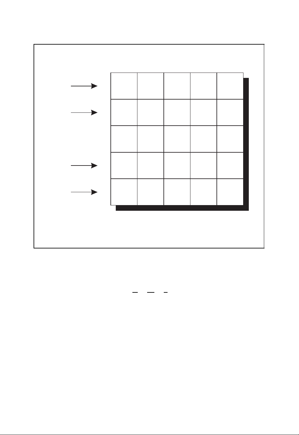
ALGEBRAIC CODING THEORY 45

Code interleaving of a linear block code

···b

b

1,0

b

2,0

.
.
.

b

t−1,0

b

t,0

t,0b1,1b2,1

b

1

b

2

.
.
.

b

t−1

b

t

■ Resulting code word of length nt



b

= b

1,0b2,0

Figure 2.26: Code interleaving of a linear block code B(n,k,d)

b

1,1

b

2,1

.
.
.

b

t−1,1

b

t,1

···b

t,1

...

...

.

...

...

···b

1,n−1b2,n−1

b

1,n−2

b

2,n−2

.

.

.

.
.

b

t−1,n−2bt−1,n−1

b

t,n−2

···b

b

b

b

t,n−1

1,n−1

2,n−1

.
.
.

t,n−1

(2.36)

Neither the code rate

nor the minimum Hamming distance d



k



=

R

=



n



= d are changed. The latter means that the error

kt

nt

k

=

= R

n

detection and error correction capabilities of the linear block code B(n,k,d) with respect
to independent errors are not improved by the interleaving step. However, error bursts
consisting of 
the linear block code B(n,k,d) is capable of correcting up to e

neighbouring errors within the received word can now be corrected. If

burst

errors, the interleaved

cor

code is capable of correcting error bursts up to length

= e



burst

cor

t

with interleaving depth t . This is achieved by spreading the error burst in the interleaved



code word b

errors occurs. In this way, the code words bjcan be corrected by the original code

e

cor

B(n,k,d) without error if the length of the error burst does not exceed e

onto t different code words bjsuch that in each code word a maximum of

t.

cor

46 ALGEBRAIC CODING THEORY

For practical applications it has to be observed that this improved correction of error

bursts comes along with an increased latency for the encoding and decoding steps.

Plotkin’s (u|v) Code Construction

In contrast to the aforementioned code constructions, the (u|v) code construction originally
proposed by Plotkin takes two linear block codes B(n
code word lengths n
distances d

and d2. For simplification, we fill the code words of the block code with smaller

1

and n2, information word lengths k1and k2and minimum Hamming

1

1,k1,d1

) and B(n2,k2,d2) with

code word length by an appropriate number of zeros. This step is called zero padding. Let u
and v be two arbitrary code words thus obtained from the linear block codes B(n
and B(n

2,k2,d2

) respectively.12Then we have









b

0,...,0,n

1

1<n2

1,k1,d1

u =

b1,n

1

≥ n

2

)

and

v =



,n

b

2







b

0,...,0,n

2

1<n2

≥ n

1

2

with the arbitrarily chosen code words b1∈ B(n1,k1,d1) and b2∈ B(n2,k2,d2). We now
identify the code words u and v with the original codes B(n
we write u ∈ B(n

1,k1,d1

) and v ∈ B(n2,k2,d2). The code resulting from Plotkin’s (u|v)

1,k1,d1

) and B(n2,k2,d2), i.e.

code construction is then given by

(n,k,d

B

) ={(u|u + v) : u ∈ B(n1,k1,d1) ∧ v ∈ B(n2,k2,d2)}.

This code construction creates all vectors of the form (u|u + v) by concatenating all possible
vectors u and u + v with u ∈ B(n

1,k1,d1

) and v ∈ B(n2,k2,d2). The resulting code is

characterised by the following code parameters



n

= 2 max{n1,n



k

= k1+ k2,



= min{2 d1,d

d

}

,

2

}

.

2

2.2.8 Examples of Linear Block Codes

In this section we will present some important linear block codes. In particular, we will
consider the already introduced repetition codes, parity-check codes and Hamming codes.
Furthermore, simplex codes and Reed–Muller codes and their relationships are discussed
(Berlekamp, 1984; Bossert, 1999; Lin and Costello, 2004; Ling and Xing, 2004).

12

In the common notation of Plotkin’s (u |v) code construction the vector u does not correspond to the infor-

mation vector.

ALGEBRAIC CODING THEORY 47

Repetition code

■ The repetition code B(n, 1,n)repeats the information symbol u

vector b = (b

■ Minimum Hamming distance

0,b1

,...,b

), i.e.

n−1

b

= b1=···=b

0

n−1

= u

0

in the code

0

(2.37)

d = n (2.38)

■ Code rate

R =

1

n

(2.39)

Figure 2.27: Repetition code

Repetition Codes

We have already introduced the binary triple repetition code in Section 1.3 as a simple
introductory example of linear block codes. In this particular code the binary information
symbol 0 or 1 is transmitted with the binary code word 000 or 111 respectively. In general,
a repetition code over the alphabet F
n-dimensional code word b = (u

assigns to the q-nary information symbol u0the

q

,...,u0). Trivially, this block code is linear. The

0,u0

minimum Hamming distance is

d = n.

Therefore, the repetition code in Figure 2.27 is a linear block code B(n, 1,n) that is able to
detect e

= d − 1 = n − 1 errors or to correct e

det

=(d − 1)/2=(n − 1)/2 errors.

cor

The code rate is

1

R =

.

n

For the purpose of error correction, the minimum distance decoding can be implemented by
a majority decoding scheme. The decoder emits the information symbol ˆu

which appears

0

most often in the received word.

The weight distribution of a repetition code is simply given by

W(x)= 1 + (q − 1)x

n

.

Although this repetition code is characterised by a low code rate R, it is used in some
communication standards owing to its simplicity. For example, in the short-range wireless
communication system Bluetooth

TM

a triple repetition code is used as part of the coding

scheme of the packet header of a transmitted baseband packet (Bluetooth, 2004).

48 ALGEBRAIC CODING THEORY

Parity-check code

■ The parity-check code B(n, n −1, 2) attaches a parity-check symbol so

that the resulting code vector b = (b

+ b1+···+b

b

0

■ Minimum Hamming distance

n−1

= 0, i.e.

b

n−1

=−(u0+ u1+···+u

d = 2 (2.41)

0,b1

,...,b

) fulfils the condition

n−1

) (2.40)

n−2

■ Code rate

R =

n − 1

n

= 1 −

1

n

(2.42)

Figure 2.28: Parity-check code

Parity-Check Codes

Starting from the information word u = (u

0,u1

,...,u

) with ui∈ Fq,aparity-check

k−1

code attaches a single parity-check symbol to the information word u as illustrated in
Figure 2.28. The n = (k + 1)-dimensional code word

is given by b
such that

b = (b

= uifor 0 ≤ i ≤ k − 1, and the parity-check symbol bkwhich is chosen

i

0,b1

,...,b

k



n−2,bn−1

) = (b0,b1,...,b

k−1,bk

)

bi= b0+ b1+···+bk= 0

i=0

is fulfilled. Over the finite field F

=−(u0+ u1+···+u

b

k

we have

q

k−1

) =−

k−1



i=0

ui.

In the case of a binary parity-check code over the alphabet F

, the parity-check bit bkis

2

chosen such that the resulting code word b is of even parity, i.e. the number of binary
symbols 1 is even. The parity-check code is a linear block code B(k +1,k,2) with a
minimum Hamming distance d = 2. This code is capable of detecting e

= d − 1 = 1

det

error. The correction of errors is not possible. The code rate is

R =

k

k + 1

=

n − 1

n

= 1 −

1

.

n

ALGEBRAIC CODING THEORY 49

The error detection is carried out by checking whether the received vector r = (r

,...,r

r

1

) fulfils the parity-check condition

n−1

n−1



ri= r0+ r1+···+r

i=0

n−1

= 0.

If this condition is not met, then at least one error has occurred.

The weight distribution of a binary parity-check code is equal to





n

2

+

x4+···+x

4

n

W(x)= 1 +





n

x

2

for an even code word length n and



W(x)= 1 +



n

x

2





n

2

+

x4+···+nx

4

n−1

for an odd code word length n. Binary parity-check codes are often applied in simple serial
interfaces such as, for example, UART (Universal Asynchronous Receiver Transmitter).

Hamming Codes

Hamming codes can be defined as binary or q -nary block codes (Ling and Xing, 2004).
In this section we will exclusively focus on binary Hamming codes, i.e. q = 2. Origi­nally, these codes were developed by Hamming for error correction of faulty memory
entries (Hamming, 1950). Binary Hamming codes are most easily defined by their corres­ponding parity-check matrix. Assume that we want to attach m parity-check symbols to an
information word u of length k. The parity-check matrix is obtained by writing down all

m-dimensional non-zero column vectors. Since there are n = 2

m

− 1 binary column vectors

of length m, the parity-check matrix



10101010··· 01010101



01100110··· 00110011





00011110··· 00001111





00000001··· 11111111





.
.



.





00000000··· 11111111

.

.

.

.

.

.

.

.

.

.

.

.

.

.

.

.

.

.

.

.

.

.

.

.

.

.

.

.

.

.

.

.

.

.

.

.

.

.

.

.

.

.

















.

.

.

.



.

.





00000000··· 11111111

,

0

m

is of dimension m × (2

− 1). By suitably rearranging the columns, we obtain the

(n − k) ×n or m ×n parity-check matrix







H =B

n−k,k

I

n−k

of the equivalent binary Hamming code. The corresponding k ×n generator matrix is then
given by

G =I





− B

k

T

n−k,k



.

50 ALGEBRAIC CODING THEORY

Because of the number of columns within the parity-check matrix H, the code word length
of the binary Hamming code is given by n = 2

m

binary information symbols k = n −m = 2

− m − 1. Since the columns of the parity-

m

− 1 = 2

n−k

− 1 with the number of

check matrix are pairwise linearly independent and there exist three columns which sum
up to the all-zero vector, the minimum Hamming distance of the binary Hamming code is

13

d = 3.
B(2

i.e. the binary Hamming code is perfect because it fulfils the sphere packing bound.
the binary Hamming code B(2

The binary Hamming code can therefore be characterised as a linear block code

m

− 1, 2m− m − 1, 3) that is able to detect e

n−k

Because of n = 2

− 1 and e

m

= 1 we have

cor





e

cor



n

= 1 + n = 2

i

i=0

− 1, 2m− m − 1, 3) only depends on the number of parity

= 2 errors or to correct e

det

n−k

,

= 1 error.

cor

14

Since

symbols m, we also call this code H(m) with the code parameters

m

n = 2

k = 2

− 1,

m

− m − 1,

d = 3.

For a binary Hamming code the decoding of an erroneously received vector r = b + e with
error vector e of weight wt(e) = 1 can be carried out by first calculating the syndrome

T

s

= HrT= He

T

which is then compared with all columns of the parity-check matrix H. If the non-zero

T

syndrome s

agrees with the j th column vector, the error vector e must have its single

non-zero component at the jth position. The received vector

r = (r

,...,r

0

j−1,rj,rj+1

,...,r

n−1

)

can therefore be decoded into the code word

ˆ

by calculatingˆb

= rj+ 1.

j

b = (r

,...,r

0

j−1,rj

+ 1,r

j+1

,...,r

n−1

)

The weight distribution W(x) of the binary Hamming code H(m) is given by

W(x)=

The coefficients w



1

n + 1

can be recursively calculated according to

i



iw

=

i

(1 +x)

n

i −1

n

+ n(1 −x)



− w

i−1

(n+1)/2

− (n − i +2)w

(1 +x)

i−2

(n−1)/2



.

with w0= 1 and w1= 0. Figure 2.29 summarises the properties of the binary Hamming
code H(m).

13

In the given matrix the first three columns sum up to the zero column vector of length m.

14

There are only two other non-trivial perfect linear codes, the binary Golay code B(23, 12, 7) with n = 23,

k = 12 and d = 7 and the ternary Golay code B(11, 6, 5) with n =11, k = 6 and d = 5. The extended binary
Golay code has been used, for example, for the Voyager 1 and 2 spacecrafts in deep-space communications.

ALGEBRAIC CODING THEORY 51

Binary Hamming code

■ The binary Hamming code H(m) is a perfect single-error correcting code

with parity-check-matrix H consisting of all 2

m

− 1 non-zero binary column

vectors of length m.

■ Code word length

■ Minimum Hamming distance

n = 2

m

− 1 (2.43)

d = 3 (2.44)

■ Code rate

R =

m

2

2m− 1

− m − 1
= 1 −

m

2m− 1

(2.45)

Figure 2.29: Binary Hamming code H(m) = B(2m− 1, 2m− m − 1, 3)

The extended binary Hamming code H



(m) is obtained from the binary Hamming

code H(m) by attaching to each code word an additional parity-check symbol such that
the resulting code word is of even parity. The corresponding non-systematic parity-check
matrix is equal to



10101010··· 01010101



01100110··· 00110011





00011110··· 00001111





00000001··· 11111111





.

.

.

.

.

.

.

.

.

.

.

.



.

.





00000000··· 11111111





00000000··· 11111111

.

.

.

.

.

.

.

.

.

.

.

.

.

.

.

.

.

.

.

.

.

.

.

.

.

.

.

.

.

.

.

.
.
.



0



0





0





0



.



.

.

.

.



.

.





0





0

11111111··· 111111111

The minimum Hamming distance of the extended Hamming code is d



= 4.

Hamming codes are used, for example, in semiconductor memories such as DRAMs for

error correction of single bit errors or in the short-range wireless communication system

TM

Bluetooth

as part of the coding scheme of the packet header of a baseband packet

(Bluetooth, 2004).

Simplex Codes

The dual code of the binary Hamming code H(m) is the so-called simplex code S(m), i.e.

⊥

(m) = S (m). This binary code over the finite field F2consists of the zero code word 0

H

and 2

m

− 1 code words of code word length n and weight 2

m−1

, i.e. wt(b) = 2

m−1

for all

52 ALGEBRAIC CODING THEORY

Simplex code

■ The simplex code S(m) is the dual of the binary Hamming code H(m), i.e.

S(m) = H

■ Code word length

■ Minimum Hamming distance

■ Code rate

code words b ∈ S (m) with b = 0. The total number of code words is M = 2
word length is n = 2

which is equal to the minimum Hamming distance d = 2

⊥

(m).

m

n = 2

R =

− 1 (2.46)

m−1

d = 2

m

2m− 1

Figure 2.30: Simplex code S (m) = B(2m− 1,m,2

m

− 1. The minimum weight of the simplex code is min

m−1

owing to the linearity of the

m−1

)

∀b=0

(2.47)

(2.48)

m

and the code

wt(b) = 2

m−1

simplex code. From these considerations, the weight distribution W(x)of the simplex code

W(x)= 1 + (2

m

− 1)x

2

m−1

= 1 + nx

(n+1)/2

easily follows.

According to Figure 2.30 the binary simplex code is characterised by the code para-

meters

m

n = 2

− 1,

,

Since the simplex code S(m) = H
the m × n parity-check matrix



10101010··· 01010101



01100110··· 00110011





00011110··· 00001111





00000001··· 11111111





.

.

.

.

.

.

.

.



.





00000000··· 11111111

.

.

.

.

.

.

.

.

.

00000000··· 11111111

k = m,

m−1

d = 2

⊥

(m) is the dual of the binary Hamming code H(m),

.















.

.

.

.

.

.

.

.

.

.

.

.

.

.

.

.

.

.

.

.

.

.

.

.

.

.

.



.

.

.

.



.

.





ALGEBRAIC CODING THEORY 53

Hadamard matrix H

■ Recursive definition of 2

■ Initialisation

m

m

× 2mHadamard matrix



H

m

H

=

H

H



m−1

m−1

0

H

−H

m−1

m−1

(2.49)

= (1) (2.50)

Figure 2.31: Hadamard matrix Hm. Reproduced by permission of J. Schlembach

Fachverlag

of the Hamming code H(m) yields the generator matrix of the simplex code S(m).If
required, the generator matrix can be brought into the systematic form

G =I





A

m

m,n−m



.

There exists an interesting relationship between the binary simplex code S (m) and the
so-called Hadamard matrix H

with the initialisation H

. This 2m× 2mmatrix is recursively defined according to

m

H

= (1). In Figure 2.31 the Hadamard matrix Hmis illustrated

0



H

=

m

m−1

H

m−1

−H



H

m−1

m−1

for 2 ≤ m ≤ 5; a black rectangle corresponds to the entry 1 whereas a white rectangle
corresponds to the entry −1.

As an example we consider m = 2 for which we obtain the 4 × 4 matrix



1111



1 −11−1



=

H

2



11−1 −1







.



1 −1 −11

Replacing all 1s with 0s and all −1s with 1s yields the matrix



0000



0101





0011







.



0110

54 ALGEBRAIC CODING THEORY

If the first column is deleted, the resulting matrix



000



101





011









110

includes as its rows all code vectors of the simplex code S(2).

In general, the simplex code S(m) can be obtained from the 2

by first applying the mapping

H

m

m

× 2mHadamard matrix

1 → 0 and − 1 → 1

and then deleting the first column. The rows of the resulting matrix deliver all 2
words of the binary simplex code S(m).

3

As a further example we consider the 2



11111111



1 −11−11−11−1





11−1 −111−1 −1





1 −1 −111−1 −11



H

=

3



1111−1 −1 −1 −1





1 −11−1 −11−11





11−1 −1 −1 −111

× 23= 8 × 8 Hadamard matrix















.











1 −1 −11−111−1

With the mapping 1 → 0 and −1 → 1, the matrix



00000000



01010101





00110011





01100110





00001111





01011010





00111100

























01101001

m

code

follows. If we delete the first column, the rows of the resulting matrix



0000000



1010101





0110011





1100110





0001111





1011010





0111100

























1101001

3

yield the binary simplex code S(3) with code word length n = 2

3−1

Hamming distance d = 2

= 4.

− 1 = 7 and minimum

ALGEBRAIC CODING THEORY 55

Reed–Muller Codes

The Hadamard matrix can further be used for the construction of other codes. The so-called
Reed–Muller codes form a class of error-correcting codes that are capable of correcting
more than one error. Although these codes do not have the best code parameters, they
are characterised by a simple and efficiently implementable decoding strategy both for
hard-decision as well as soft-decision decoding. There exist first-order and higher-order
Reed–Muller codes, as we will explain in the following.

First-Order Reed –Muller Codes R (1,m) The binary first-order Reed –Muller code

m

R(1,m) can be defined with the help of the following m ×2
all possible 2

m

binary column vectors of length m



000000000··· 11111111



000000000··· 11111111





.

.

.

.

.

.

.

.

.

.

.

.

.

.



.

.

.





000000001··· 11111111





000011110··· 00001111





001100110··· 00110011

.

.

.

.

.

.

.

.

.

.

.

.

.

.

.

.

.

.

.

.

.

.

matrix which contains

.

.

.

.

.

.

.

.

.

.

.

.

.

.

.













.











010101010··· 01010101

By attaching the 2



as the first row, we obtain the (m + 1) × 2

G =

m

-dimensional all-one vector

11111111··· 111111111

m

generator matrix



111111111··· 11111111



000000000··· 11111111





000000000··· 11111111





.

.

.

.

.

.

.

.

.

.

.

.

.



.

.

.





000000001··· 11111111





000011110··· 00001111





001100110··· 00110011

.

.

.

.

.

.

.

.

.

.

.

.

.

.

.

.

.

.

.

.

.

.

.

.

.

.

.

.

.

.

.

.

.

.

.















.
.



.

.













010101010··· 01010101

The binary first-order Reed –Muller code R(1,m) in Figure 2.32 is characterised by the
following code parameters

m

,

n = 2

k = 1 + m,

m−1

d = 2

.

The corresponding weight distribution W(x) is given by

W(x)= 1 +2

m+1

− 2x

2

m−1

+ x

m

2

,

56 ALGEBRAIC CODING THEORY

First-order Reed–Muller code R(1,m)

■ The first-order Reed–Muller code R(1,m) isabinarycodethatisableto

correct more than one error.

■ Code word length

■ Minimum Hamming distance

■ Code rate

R =

n = 2

d = 2

1 +

m

m−1

m

2

(2.51)

(2.52)





m

1

(2.53)

Figure 2.32: First-order Reed – Muller code R(1,m)

i.e. the binary first-order Reed –Muller code R(1,m)consists of code vectors with weights

m−1

0, 2

and 2m. The hard-decision decoding of a Reed –Muller code can be carried out by

a majority logic decoding scheme.

There is a close relationship between the binary first-order Reed –Muller code R(1,m)
and the simplex code S (m) with code word length n = 2
symbols as well as the Hamming code H(m). The m × 2

m

− 1 and k = m information

m

matrix used in the construction

of the generator matrix of the first-order Reed–Muller code R(1,m) corresponds to the
parity-check matrix of the binary Hamming code H(m) with the all-zero column attached.
This parity-check matrix in turn yields the generator matrix of the simplex code S(m).
Therefore, this m ×2

m

matrix generates all code words of the simplex code S(m) with a

zero attached in the first position. The attachment of the all-one row vector to the m ×2
matrix is equivalent to adding all inverted code words to the code. In summary, the simplex
code S (m) yields the Reed–Muller code R(1,m) by attaching a zero to all code words in
the first position and adding all inverted vectors to the code (Bossert, 1999).

If we compare this code construction scheme with the relationship between simplex
codes S(m) and Hadamard matrices H
matrix

, we recognise that the rows of the 2

m



H

−H



m

m

m+1

× 2

subjected to the mapping 1 → 0 and −1 → 1 yield the code vectors of the first-order
Reed–Muller code R(1,m).

This observation in combination with the orthogonality property

m

m

H

mHm

= 2mI

m

2

ALGEBRAIC CODING THEORY 57

of the Hadamard matrix H

with the 2m× 2midentity matrix I

m

m

can be used to implement

2

a soft-decision decoding algorithm. To this end, we assume that the received vector

r = x + e

corresponds to the real-valued output signal of an AWGN channel (see also Figure 1.5)
with n-dimensional normally distributed noise vector e.

15

The bipolar signal vector x = x

with components ±1 is given by the j th row of the matrix



−H



H

m

.

m

This bipolar signal vector x is obtained from the binary code vector b by the mapping

m+1

1 →−1 and 0 → 1. With the help of the 2

-dimensional row vector

v = (0,...,0, 1, 0,...,0),

the components of which are 0 except for the j th component which is equal to 1, we can
express the bipolar signal vector according to

−H



H

m

.

m



x = v

Within the soft-decision decoder architecture the real-valued received vector r is trans­formed with the Hadamard matrix H

rH

=!v

m

= v

= v

= v

= 2mv

, leading to

m



H

−H



H

−H



H

−HmH



m

2

−2mI



−I

m

m



m

m

mHm

m

I

2

m

2

m

I

2

m

2



+ e"H

H

m



m





+ eH

+ eH

+ eH

+ eH

m

m

m

m

m

=±2mv + eHm.

j

Because of rH
ulus of all components in the transformed received vector rH

=±2mv + eHm, the soft-decision decoder searches for the largest mod-

m

. This component in con-

m

junction with the respective sign delivers the decoded signal vectorˆx or code vectorˆb.
The transform rH

can be efficiently implemented with the help of the fast Hadamard

m

transform (FHT). In Figure 2.33 this soft-decision decoding is compared with the optimal
hard-decision minimum distance decoding of a first-order Reed – Muller code R(1, 4).

15

Here, the arithmetics are carried out in the vector space Rn.

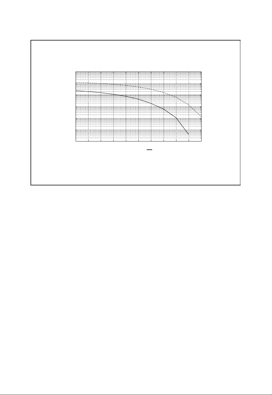
58 ALGEBRAIC CODING THEORY

Hard-decision and soft-decision decoding

0

10

Ŧ1

10

Ŧ2

10

err

Ŧ3

10

p

Ŧ4

10

Ŧ5

10

Ŧ6

10

Ŧ5 Ŧ4 Ŧ3 Ŧ2 Ŧ1 0 1 2 3 4 5

10 log

■ Comparison between hard-decision decoding and soft-decision decoding

of a binary first-order Reed – Muller code R(1, 4) with code parameters
n = 16, k = 5 and d = 8 with respect to the word error probability p

Figure 2.33: Hard-decision and soft-decision decoding of a binary first-order

Reed–Muller code R(1, 4)





E

b

10

N

0

err

The FHT is used, for example, in UMTS (Holma and Toskala, 2004) receivers for the
decoding of TFCI (transport format combination indicator) symbols which are encoded with
the help of a subset of a second-order Reed–Muller code R(2, 5) with code word length

5

n = 2

= 32 (see, for example, (3GPP, 1999)). Reed–Muller codes have also been used

in deep-space explorations, e.g. the first-order Reed–Muller code R(1, 5) in the Mariner
spacecraft (Costello et al., 1998).

Higher-order Reed–Muller Codes R(r, m) The construction principle of binary first-
order Reed–Muller codes R(1,m) can be extended to higher-order Reed –Muller codes
R(r, m). For this purpose we consider the 5 × 16 generator matrix

G =



1111111111111111



0000000011111111





0000111100001111





0011001100110011













0101010101010101

of a first-order Reed – Muller code R(1, 4). The rows of this matrix correspond to the
Boolean functions f

, f1, f2, f3and f4shown in Figure 2.34. If we also consider the

0

ALGEBRAIC CODING THEORY 59

Boolean functions for the definition of a first-order Reed–Muller
code R(1, 4)

x10000000011111111

0000111100001111

x

2

0011001100110011

x

3

0101010101010101

x

4

f01111111111111111
f

0000000011111111

1

0000111100001111

f

2

0011001100110011

f

3

0101010101010101

f

4

■ Boolean functions with x

1,x2,x3,x4

f

0(x1,x2,x3,x4

f

1(x1,x2,x3,x4

f2(x1,x2,x3,x4) = x

f3(x1,x2,x3,x4) = x

f4(x1,x2,x3,x4) = x

∈{0, 1}

) = 1

) = x

1

2

3

4

Figure 2.34: Boolean functions for the definition of a first-order Reed–Muller code

R(1, 4)

additional Boolean functions f

1,2

, f

1,3

, f

1,4

, f

2,3

, f

2,4

and f

in Figure 2.35, we obtain

3,4

the 11 × 16 generator matrix

G =



1111111111111111



0000000011111111





0000111100001111





0011001100110011





0101010101010101





0000000000001111





0000000000110011





0000000001010101





0000001100000011





0000010100000101





































0001000100010001

of the second-order Reed – Muller code R(2, 4) from the table in Figure 2.35.

60 ALGEBRAIC CODING THEORY

Boolean functions for the definition of a second-order
Reed–Muller code R(2, 4)

x10000000011111111

0000111100001111

x

2

0011001100110011

x

3

0101010101010101

x

4

f01111111111111111
f

0000000011111111

1

0000111100001111

f

2

0011001100110011

f

3

0101010101010101

f

4

f

0000000000001111

1,2

0000000000110011

f

1,3

0000000001010101

f

1,4

f

0000001100000011

2,3

0000010100000101

f

2,4

0001000100010001

f

3,4

■ Boolean functions with x

1,x2,x3,x4

f

1,2(x1,x2,x3,x4

f

1,3(x1,x2,x3,x4

f

1,4(x1,x2,x3,x4

f

2,3(x1,x2,x3,x4

f

2,4(x1,x2,x3,x4

f

3,4(x1,x2,x3,x4

∈{0, 1}

) = x1x

) = x1x

) = x1x

) = x2x

) = x2x

) = x3x

2

3

4

3

4

4

Figure 2.35: Boolean functions for the definition of a second-order Reed–Muller code

R(2, 4)

This code construction methodology can be extended to the definition of higher-order
Reed–Muller codes R(r, m) based on the Boolean functions

i

i

2

2

···x

i

m

m

1

x

x

1

with

+ i2+···+im≤ r

i

1

ALGEBRAIC CODING THEORY 61

Reed–Muller code R(r, m)

■ The Reed – Muller code R(r, m) is a binary code that is able to correct more

than one error.

■ Code word length

■ Minimum Hamming distance

■ Code rate

R =

1 +



m

n = 2

d = 2

+

1

m

m−r



m

+···+

2

m

2

(2.54)

(2.55)





m

r

(2.56)

Figure 2.36: Reed –Muller code R (r, m)

and i

∈{0, 1}. These Boolean functions are used to define the rows of the generator matrix

j

G. The resulting Reed–Muller code R(r, m) of order r in Figure 2.36 is characterised by
the following code parameters

m

n = 2

k = 1 +

d = 2

m−r

,



+

m

1

m

2



+ ...+





m

,

r

.

There also exists a recursive definition of Reed – Muller codes based on Plotkin’s (u|v)
code construction (Bossert, 1999)

R(r +1,m+ 1) ={(u|u + v) : u ∈ R(r + 1,m)∧ v ∈ R(r, m)}.

The code vectors b = (u|u + v) of the Reed–Muller code R(r +1,m+ 1) are obtained
from all possible combinations of the code vectors u ∈ R(r +1,m) of the Reed – Muller
code R(r +1,m) and v ∈ R(r, m) of the Reed–Muller code R(r, m). Furthermore, the
dual code of the Reed–Muller code R(r, m) yields the Reed –Muller code

⊥

R

(r, m) = R(m − r − 1,m).

Finally, Figure 2.37 summarises the relationship between first-order Reed–Muller codes
R(1,m), binary Hamming codes H(m) and simplex codes S (m) (Bossert, 1999).

62 ALGEBRAIC CODING THEORY

First-order Reed – Muller codes R(1,m), binary Hamming codes
H(m) and simplex codes S(m)

■ Reed–Muller code R(1,m)and extended Hamming code H

⊥

⊥

⊥



(m)

(m)

(m)

(i) R(1,m) = H



(m) = R⊥(1,m)= R(m − 2,m)

(ii) H

■ Hamming code H (m) and simplex code S(m)

(i) S(m) = H

(ii) H(m) = S

■ Simplex code S (m) and Reed–Muller code R(1,m)



(m)

(i) S(m) → R(1,m)

1. All code words from S(m) are extended by the first position 0.

2. R(1,m) consists of all corresponding code words including the

inverted code words.

(ii) R(1,m) → S (m)

1. All code words with the first component 0 are removed from

R(1,m).

2. The first component is deleted.

Figure 2.37: Relationship between first-order Reed–Muller codes R(1,m), binary

Hamming codes H(m) and simplex codes S (m)

2.3 Cyclic Codes

Linear block codes make it possible efficiently to implement the encoding of information
words with the help of the generator matrix G. In general, however, the problem of decoding
an arbitrary linear block code is difficult. For that reason we now turn to cyclic codes as
special linear block codes. These codes introduce further algebraic properties in order to
be able to define more efficient algebraic decoding algorithms (Berlekamp, 1984; Lin and
Costello, 2004; Ling and Xing, 2004).

2.3.1 Definition of Cyclic Codes

A cyclic code is characterised as a linear block code B(n,k,d)with the additional property
that for each code word

b = (b

0,b1

,...,b

n−2,bn−1

)

ALGEBRAIC CODING THEORY 63

all cyclically shifted words

(b

n−1,b0

(b

n−2,bn−1

(b

2,b3

(b

1,b2

, ... , b

, ... , b

.
.
.

, ... ,b0,b1),

, ... ,b

n−3,bn−2

n−4,bn−3

n−1,b0

),

),

)

are also valid code words of B(n,k,d) (Lin and Costello, 2004; Ling and Xing, 2004). This

n

property can be formulated concisely if a code word b ∈ F

b(z) = b

+ b1z +···+b

0

n−2

z

n−2

is represented as a polynomial

q

n−1

z

n−1

+ b

over the finite field Fq.16A cyclic shift

,...,b

(b

0,b1

of the code polynomial b(z) ∈ F

+ b1z +···+b

b

0

n−2

z

n−2

n−2,bn−1

[z] can then be expressed as

q

+ b

n−1

) → (b

n−1

z

→ b

n−1,b0,b1

n−1

,...,b

n−2

+ b0z + b1z2+···+b

)

n−1

z

n−2

.

Because of

+ b0z + b1z2+···+b

b

n−1

n−2

n−1

z

= zb(z)−b



n−1



n

− 1

z

and by observing that a code polynomial b(z) is of maximal degree n −1, we represent

n

n−2

− 1, i.e.

n−1

z

≡ zb(z) mod zn− 1.

the cyclically shifted code polynomial modulo z

+ b0z + b1z2+···+b

b

n−1

Cyclic codes B(n,k,d) therefore fulfil the following algebraic property

n

b(z) ∈ B(n,k,d) ⇔ zb(z) mod z

− 1 ∈ B(n,k,d).

For that reason – if not otherwise stated – we consider polynomials in the factorial ring

[z]/(zn− 1). Figure 2.38 summarises the definition of cyclic codes.

F

q

Similarly to general linear block codes, which can be defined by the generator matrix
G or the corresponding parity-check matrix H, cyclic codes can be characterised by the
generator polynomial g(z) and the parity-check polynomial h(z), as we will show in the
following (Berlekamp, 1984; Bossert, 1999; Lin and Costello, 2004; Ling and Xing, 2004).

2.3.2 Generator Polynomial

A linear block code B(n,k,d) is defined by the k × n generator matrix







G =





16

Polynomials over finite fields are explained in Section A.3 in Appendix A.



g

0

g

1

.
.
.

g

k−1







=





g
g

g

k−1,0gk−1,1









0,0

1,0

.
.
.

g

··· g

0,1

g

··· g

1,1

.

.

.

.

.

.

··· g

k−1,n−1

0,n−1

1,n−1

.
.
.











64 ALGEBRAIC CODING THEORY

Definition of cyclic codes

■ Each code word b = (b

0,b1

,...,b

n−2,bn−1

) of a cyclic code B(n,k,d) is

represented by the polynomial

b(z) = b

■ All cyclic shifts of a code word b are also valid code words in the cyclic

+ b1z +···+b

0

n−2

z

n−2

+ b

n−1

z

n−1

(2.57)

code B(n,k,d), i.e.

b(z) ∈ B(n,k,d) ⇔ zb(z) mod z

n

− 1 ∈ B(n,k,d) (2.58)

Figure 2.38: Definition of cyclic codes

with k linearly independent basis vectors g

, g1, ..., g

0

which themselves are valid code

k−1

vectors of the linear block code B(n,k,d). Owing to the algebraic properties of a cyclic
code there exists a unique polynomial

g(z) = g

+ g1z +···+g

0

of minimal degree deg(g(z)) = n −k with g

n−k−1

z

n−k−1

= 1 such that the corresponding generator

n−k

+ g

n−k

z

n−k

matrix can be written as

G =



g

0g1



0 g





.
.



.





00··· 00··· g

0

.
.
.

··· g

··· g

.

.

.

n−k

n−k−1gn−k

.
.
.

0 ··· 00··· 00

.
.
.

··· 00··· 00

.

.

.

00··· 00··· 0 g

.
.
.

0g1

.
.
.

0

.

.

.

··· g

··· g

.
.
.

n−k

n−k−1gn−k









.
.

.



.





0

This polynomial g(z) is called the generator polynomial of the cyclic code B(n,k,d)
(Berlekamp, 1984; Bossert, 1999; Lin and Costello, 2004; Ling and Xing, 2004). The rows
of the generator matrix G are obtained from the generator polynomial g(z) and all cyclic
shifts zg(z), z

2

g(z), ..., z

k−1

g(z) which correspond to valid code words of the cyclic

code. Formally, we can write the generator matrix as

G =



g(z)



zg(z)









k−2



z

k−1

z

.
.
.

g(z)
g(z)









.







ALGEBRAIC CODING THEORY 65

In view of the encoding rule for linear block codes b = uG, we can write

(u

0,u1

,...,u

k−1



g(z)



zg(z)





)





k−2



z

k−1

z

.
.
.

g(z)
g(z)









= u







g(z) +u1zg(z) +···+u

0

k−1

z

k−1

g(z).

For the information word u = (u
polynomial

u(z) = u

, ··· ,u

0,u1

+ u1z + u2z2+···+u

0

) we define the corresponding information

k−1

k−1

z

k−1

.

This information polynomial u(z) can thus be encoded according to the polynomial multi­plication

b(z) = u(z) g(z).

Because of b(z) = u(z) g(z), the generator polynomial g(z) divides every code polyno­mial b(z).Ifg(z) does not divide a given polynomial, this polynomial is not a valid code
polynomial, i.e.

g(z) |b(z) ⇔ b(z) ∈ B(n,k,d)

or equivalently

b(z) ≡ 0 mod g(z) ⇔ b(z) ∈ B(n,k,d).

The simple multiplicative encoding rule b(z) = u(z) g(z), however, does not lead to a
systematic encoding scheme where all information symbols are found at specified positions.

By making use of the relation b(z) ≡ 0 modulo g(z), we can derive a systematic
encoding scheme. To this end, we place the k information symbols u

in the k upper

i

positions in the code word

b = (b

The remaining code symbols b

,...,b

0,b1

, b1, ..., b

0

n−k−1,u0,u1

n−k−1

,...,u

  

=u

k−1

).

correspond to the n −k parity-check

symbols which have to be determined. By applying the condition b(z) ≡ 0 modulo g(z) to
the code polynomial

b(z) = b

+ b1z +···+b

0

= b0+ b1z +···+b

n−k−1

n−k−1

n−k−1

z

n−k−1

z

+ u0z

n−k

+ z

n−k

u(z)

+ u1z

n−k+1

+···+u

k−1

z

n−1

we obtain

+ b1z +···+b

b

0

The parity-check symbols b

, b1, ..., b

0

division of the shifted information polynomial z

n−k−1

n−k−1

z

n−k−1

n−k

≡−z

u(z) mod g(z).

are determined from the remainder of the

n−k

u(z) by the generator polynomial g(z).

Figure 2.39 summarises the non-systematic and systematic encoding schemes for cyclic
codes.

It can be shown that the binary Hamming code in Figure 2.29 is equivalent to a cyclic
code. The cyclic binary (7, 4) Hamming code, for example, is defined by the generator
polynomial

g(z) = 1 +z +z

3

∈ F2[z].

66 ALGEBRAIC CODING THEORY

Generator polynomial

■ The cyclic code B(n,k,d)is defined by the unique generator polynomial

g(z) = g

+ g1z +···+g

0

of minimal degree deg(g(z)) = n −k with g

■ Non-systematic encoding

n−k−1

n−k

n−k−1

z

+ g

= 1.

n−k

z

n−k

(2.59)

b(z) = u(z) g(z) (2.60)

■ Systematic encoding

b

+ b1z +···+b

0

n−k−1

n−k−1

z

≡−z

n−k

u(z) mod g(z) (2.61)

Figure 2.39: Encoding of a cyclic code with the help of the generator polynomial g(z)

The non-systematic and systematic encoding schemes for this cyclic binary Hamming code
are illustrated in Figure 2.40.

Cyclic Redundancy Check

With the help of the generator polynomial g(z) of a cyclic code B(n,k,d), the so-called
cyclic redundancy check (CRC) can be defined for the detection of errors (Lin and Costello,

2004). Besides the detection of e

= d − 1 errors by a cyclic code B(n,k,d) with min-

det

imum Hamming distance d, cyclic error bursts can also be detected. With a generator
polynomial g(z) of degree deg(g(z)) = n − k, all cyclic error bursts of length



≤ n −k

burst

can be detected (Jungnickel, 1995). This can be seen by considering the error model r(z) =
b(z) + e(z) with the received polynomial r(z), the code polynomial b(z) and the error
polynomial e(z) (see also Figure 2.46). Errors can be detected as long as the parity-check
equation

g(z) |r(z) ⇔ r(z) ∈ B(n,k,d)

of the cyclic code B(n,k,d) is fulfilled. Since g(z)|b(z), all errors for which the error
polynomial e(z) is not divisible by the generator polynomial g(z) can be detected. As long
as the degree deg(e(z)) is smaller than deg(g(z)) = n − k, the error polynomial e(z) cannot

i

burst

e(z)

the

be divided by the generator polynomial. This is also true if cyclically shifted variants z
of such an error polynomial are considered. Since for an error burst of length 
degree of the error polynomial is equal to 

deg(e(z)) = 

burst

− 1, the error detection is possible if

burst

− 1 <n−k = deg(g(z)).

ALGEBRAIC CODING THEORY 67

Cyclic binary Hamming code

■ The generator polynomial of a cyclic binary (7,4) Hamming code is given

by

g(z) = 1 +z +z

3

∈ F2[z]

+ z

6

3

yields

3

yields

■ Non-systematic encoding of the information polynomial u(z) = 1 +z



b(z) = u(z) g(z) =1 +z

■ Systematic encoding of the information polynomial u(z) = 1 + z

3(z3

z

+ 1) ≡ z2+ z mod 1 + z + z

3

1 +z + z



3

= 1 + z +z

4

3

leading to the code polynomial

b(z) = z + z

2

+ z3+ z

6

Figure 2.40: Cyclic binary (7, 4) Hamming code

Figure 2.41 gives some commonly used CRC generator polynomials (Lin and Costello,

2004).

2.3.3 Parity-Check Polynomial

It can be shown that the generator polynomial g(z) of a cyclic code divides the polynomial

n

− 1 in the polynomial ring Fq[z], i.e.

z

g(z) h(z) = z

n

− 1.

In the factorial ring F

The polynomial

[z]/(zn− 1) this amounts to g(z) h(z) = 0 or equivalently

q

n

− 1

g(z)

n

− 1.

g(z) h(z) ≡ 0 mod z

h(z) =

z

is the so-called parity-check polynomial (Berlekamp, 1984; Bossert, 1999; Lin and Costello,
2004; Ling and Xing, 2004). Since every code polynomial b(z) is a multiple of the generator
polynomial g(z), the parity-check equation can also be written as (see Figure 2.42)

n

b(z) h(z) ≡ 0 mod z

− 1 ⇔ b(z) ∈ B(n,k,d).

This parity-check equation is in correspondence with the matrix equation

T

= 0 ⇔ b ∈ B(n,k,d)

Hb

68 ALGEBRAIC CODING THEORY

Cyclic redundancy check

■ The generator polynomial g(z) can be used for the detection of errors by

making use of the cyclic redundancy check (CRC)

r(z) ≡ 0 mod g(z) ⇔ r(z) ∈ B(n,k,d) (2.62)

■ The received polynomial

r(z) = r

+ r1z +···+r

0

of the received word r = (r

0,r1

,...,r

z

n−2

n−2,rn−1

n−2

+ r

) is divided by the generator

n−1

z

n−1

polynomial g(z). If the remainder is zero, the received word is a valid code
word, otherwise transmission errors have been detected. In the so-called
ARQ (automatic repeat request) scheme, the receiver can prompt the
transmitter to retransmit the code word.

■ The following table shows some generator polynomials used for CRC.

CRC-12 g(z) = 1 +z +z2+ z3+ z4+ z
CRC-16 g(z) = 1 +z2+ z15+ z
CRC-CCITT g(z) = 1 +z5+ z12+ z

16

16

12

Figure 2.41: Cyclic redundancy check

Parity-check polynomial

■ The parity-check polynomial h(z) of a cyclic code B(n,k,d) with generator

polynomial g(z) is given by

n

− 1

h(z) =

z

g(z)

(2.63)

(2.64)

■ Parity-check equation

b(z) h(z) ≡ 0 mod z

Figure 2.42: Parity-check polynomial h(z)

n

− 1 ⇔ b(z) ∈ B(n,k,d) (2.65)

ALGEBRAIC CODING THEORY 69

Parity-check polynomial of the cyclic binary Hamming code

■ The generator polynomial of the cyclic binary (7,4) Hamming code is given

by

g(z) = 1 +z +z

■ The parity-check polynomial of this cyclic binary Hamming code is equal

to

h(z) = 1 + z + z

Figure 2.43: Parity-check polynomial of the cyclic binary (7, 4) Hamming code

for general linear block codes. Figure 2.43 gives the parity-check polynomial of the cyclic
(7, 4) binary Hamming code.

Because of deg(g(z)) = n − k and deg(z
degree of the parity-check polynomial is given by deg(h(z)) = k. Taking into account
the normalisation g

= 1, we see that hk= 1, i.e.

n−k

3

∈ F2[z]

2

4

+ z

n

− 1) = n = deg(g(z)) +deg(h(z)), the

h(z) = h

+ h1z +···+h

0

k−1

z

k−1

+ zk.

Based on the parity-check polynomial h(z), yet another systematic encoding algorithm can

n

be derived. To this end, we make use of g(z) h(z) = z

− 1 and b(z) = u(z) g(z). This

yields

n

b(z) h(z) = u(z) g(z) h(z) = u(z)z

− 1=−u(z) + znu(z).

The degree of the information polynomial u(z) is bounded by deg(u(z)) ≤ k −1, whereas
the minimal exponent of the polynomial z
does not contain the exponentials z

n

k

u(z) is n. Therefore, the polynomial b(z) h(z)

, z

k+1

, ..., z

n−1

. This yields the n − k parity-check

equations

b

n−k−2hk

b

n−k−1hk

b

b

0hk

1hk

+ b

+ b

+ b1h

+ b2h

n−k−1hk−1

n−khk−1

+···+bkh0= 0,

k−1

+···+b

k−1

+···+b

+···+b

k+1h0

.
.
.

n−2h0

n−1h0

= 0,

= 0,

= 0

which can be written as the discrete convolution

k



hjb

j=0

i−j

= 0

70 ALGEBRAIC CODING THEORY

for k ≤ i ≤ n −1. This corresponds to the matrix equation Hb

T

= 0 for general linear

block codes with the (n −k) × n parity-check matrix









.
.

.



.





0

H =



h

khk−1



0 h





.
.



.





00··· 00··· h

··· h00 ··· 00··· 00

··· h1h0··· 00··· 00

k

.
.
.

.

.

.

.

.
.
.

.

.

.

.

.

00··· 00··· 0 h

.
.
.

khk−1

.
.
.

k

.

.

.

.

.

.

··· h00

··· h1h

For the systematic encoding scheme the k code symbols b
equal to the respective information symbols u

, u1, ..., u

0

system of equations taking into account the normalisation h

b

n−k−2

b

n−k−1

+ b1h

b

0

b

1

+ b

n−k−1hk−1

+ b

+ b2h

n−khk−1

+···+bkh0= 0,

k−1

+···+b

k−1

+···+b

+···+b

k+1h0

.
.
.

n−2h0

n−1h0

which is recursively solved for the parity-check symbols b
leads to the systematic encoding scheme

b

n−k−1

b

n−k−2

=−(b

=−(b

.
.
.

b

=−(b2h

1

b

=−(b1h

0

n−khk−1

n−k−1hk−1

+···+b

+···+b

k−1

+···+bkh

k−1

n−1h0

+···+b

k+1h0

)

0

2.3.4 Dual Codes

, b

n−k

. This yields the following

k−1

= 1

k

n−k+1

, ..., b

= 0,

= 0,

= 0

n−k−1

)

n−2h0

,

)

, b

,

)

, ..., b1, b0. This

n−k−2

,

.

n−1

are set

Similarly to general linear block codes, the dual code B⊥(n,k,d) of the cyclic code
B(n,k,d) with generator polynomial g(z) and parity-check polynomial h(z) can be defined
by changing the role of these polynomials (Jungnickel, 1995). Here, we have to take into
account that the generator polynomial must be normalised such that the highest exponent
has coefficient 1. To this end, we make use of the already derived (n − k) × n parity-check
matrix









.
.



.





0

H =



h

khk−1



0 h





.
.



.





00··· 00··· h

··· h00 ··· 00··· 00

··· h1h0··· 00··· 00

k

.
.
.

.

.

.

.

.
.
.

.

.

.

.

.

00··· 00··· 0 h

.
.
.

khk−1

.
.
.

k

.

.

.

.

.

.

··· h00

··· h1h

ALGEBRAIC CODING THEORY 71

of a cyclic code. By comparing this matrix with the generator matrix

G =



g

0g1



0 g





.
.



.





00··· 00··· g

0

.
.
.

··· g

··· g

.

.

.

n−k

n−k−1gn−k

.
.
.

0 ··· 00··· 00

.
.
.

··· 00··· 00

.

.

00··· 00··· 0 g

.

.
.
.

0

.

··· g

··· g

.

.

.

0g1

.

.

.
.
.

n−k

n−k−1gn−k









.
.



.





0

of a cyclic code, we observe that, besides different dimensions and a different order of
the matrix elements, the structure of these matrices is similar. With this observation, the
generator polynomial g

⊥

(z) of the dual cyclic code B⊥(n,k,d) can be obtained from the

reversed and normalised parity-check polynomial according to

k−1

0

k−1

h

0

g

⊥

(z) =

+ h

h

k

h0+ h1z−1+···+h

k

= z

h(z−1)

k

= z

z +···+h1z

k−1

.

h

0

h

Figure 2.44 summarises the definition of the dual cyclic code B

+ h0z

−k+1

z

k

+ hkz

⊥(n,k,d

−k

) of the cyclic

code B(n,k,d).

2.3.5 Linear Feedback Shift Registers

As we have seen, the systematic encoding of a cyclic code can be carried out by dividing the
shifted information polynomial z

n−k

u(z) by the generator polynomial g(z). The respective

Dual cyclic code

■ Let h(z) be the parity-check polynomial of the cyclic code B(n,k,d).

■ The dual code B

polynomial

⊥(n,k,d

) is the cyclic code defined by the generator

⊥

g

(z) = z

h(z−1)

k

h

0

(2.66)

■ For cyclic binary codes h

= 1, and therefore

0

⊥

g

(z) = zkh(z−1) (2.67)

Figure 2.44: Dual cyclic code B⊥(n,k,d) of the cyclic code B(n,k,d)

72 ALGEBRAIC CODING THEORY

remainder yields the sought parity-check symbols. As is well known, polynomial division
can be carried out with the help of linear feedback shift registers. Based on these linear
feedback shift registers, efficient encoding and decoding architectures for cyclic codes can
be derived (Berlekamp, 1984; Lin and Costello, 2004).

Encoding Architecture

For the information polynomial

u(z) = u

+ u1z +···+u

0

k−2

z

k−2

+ u

k−1

z

k−1

and the generator polynomial

g(z) = g

+ g1z +···+g

0

n−k−1

n−k−1

z

+ z

n−k

the encoder architecture of a cyclic code over the finite field Fqcan be derived by mak­ing use of a linear feedback shift register with n −k registers as shown in Figure 2.45
(Neubauer, 2006b).

After the q-nary information symbols u

k−1

, u

, ···, u1, u0have been shifted into

k−2

the linear feedback shift register, the registers contain the components of the remainder

s(z) = s

≡ z

+ s1z +···+s

0

n−k

u(z) mod g(z).

n−k−2

n−k−2

z

+ s

n−k−1

n−k−1

z

Besides an additional sign, this term yields the remainder that is needed for the systematic
encoding of the information polynomial u(z). Therefore, after k clock cycles, the linear
feedback shift register contains the negative parity-check symbols within the registers that
can subsequently be emitted by the shift register. In summary, this encoding architecture
yields the code polynomial

b(z) = z

n−k

u(z) − s(z).

Decoding Architecture

The linear feedback shift register can also be used for the decoding of a cyclic code. Starting
from the polynomial channel model illustrated in Figure 2.46

r(z) = b(z) + e(z)

with the error polynomial

e(z) = e

+ e1z + e2z2+···+e

0

n−1

z

n−1

the syndrome polynomial is defined according to

s(z) ≡ r(z) mod g(z).

The degree of the syndrome polynomial s(z) is bounded by deg(s(z)) ≤ n −k −1.

ALGEBRAIC CODING THEORY 73

Encoder architecture for a cyclic code

...

+

■ The sequence of information symbols u

+

g

0

+ + +

g

1

...

u0u1···u

+

k−2uk−1

k−1

g

n−k−1

, u

+

, ···, u1, u0is shifted into

k−2

−1

the linear feedback shift register within the first k clock cycles (switch
positions according to the solid lines).

■ At the end of the kth clock cycle the registers contain the negative parity-

check symbols.

■ The parity-check symbols are emitted during the next n − k clock cycles

(switch positions according to the dashed lines).

Figure 2.45: Encoding of a cyclic code with a linear feedback shift register. Reproduced

by permission of J. Schlembach Fachverlag

If the received polynomial r(z) is error free and therefore corresponds to the transmitted
code polynomial b(z), the syndrome polynomial s(z) is zero. If, however, the received
polynomial r(z) is disturbed, the syndrome polynomial

s(z) ≡ r(z) ≡ b(z) + e(z) ≡ e(z) mod g(z)

exclusively depends on the error polynomial e(z). Because of s(z) ≡ r(z) modulo g(z), the
syndrome polynomial is obtained as the polynomial remainder of the division of the received
polynomial r(z) by the generator polynomial g(z). This division operation can again be car-
ried out by a linear feedback shift register as illustrated in Figure 2.47 (Neubauer, 2006b).
Similarly to the syndrome decoding of linear block codes, we obtain the decoder archi­tecture shown in Figure 2.48 which is now based on a linear feedback shift register and a
table look-up procedure (Neubauer, 2006b). Further information about encoder and decoder
architectures based on linear feedback shift registers can be found elsewhere (Berlekamp,
1984; Lin and Costello, 2004).

74 ALGEBRAIC CODING THEORY

Polynomial channel model

b(z)

+

r(z)

e(z)

■ The transmitted code polynomial b(z) is disturbed by the error polynomial

e(z).

■ The received polynomial r(z) is given by

r(z) = b(z) + e(z) (2.68)

■ The syndrome polynomial

s(z) ≡ r(z) mod g(z) (2.69)

exclusively depends on the error polynomial e(z).

Figure 2.46: Polynomial channel model

2.3.6 BCH Codes

We now turn to the so-called BCH codes as an important class of cyclic codes (Berlekamp,
1984; Bossert, 1999; Lin and Costello, 2004; Ling and Xing, 2004). These codes make it
possible to derive an efficient algebraic decoding algorithm. In order to be able to define
BCH codes, we first have to introduce zeros of a cyclic code.

Zeros of Cyclic Codes

A cyclic code B(n,k,d)over the finite field F

is defined by a unique generator polynomial

q

g(z) which divides each code polynomial b(z) ∈ B(n,k,d) according to g(z) |b(z) or

equivalently

b(z) ≡ 0 mod g(z).

The generator polynomial itself is a divisor of the polynomial z

n

g(z) h(z) = z

17

For further details about the arithmetics in finite fields the reader is referred to Section A.3 in Appendix A.

− 1.

17

n

− 1, i.e.

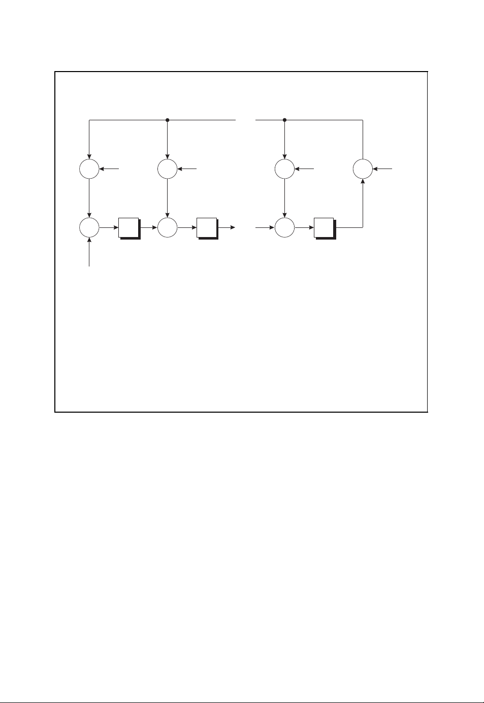
ALGEBRAIC CODING THEORY 75

Decoder architecture for a cyclic code

...

+

g

0

+

r

n−1

r

n−2

.
.
.

r

0

■ The sequence of received symbols r

+

+ +

g

1

...

, r

n−1

+

n−2

g

n−k−1

, ..., r1, r0is shifted into the

+

−1

linear feedback shift register.

■ At the end of the nth clock cycle the registers contain the syndrome

polynomial coefficients s

, s1, ..., s

0

n−k−2

, s

from left to right.

n−k−1

Figure 2.47: Decoding of a cyclic code with a linear feedback shift register. Reproduced

by permission of J. Schlembach Fachverlag

In the following, we assume that the polynomial z

n

− 1 has only single zeros which is

equivalent to the condition (McEliece, 1987)

gcd(q, n) = 1.

This means that the cardinality q of the finite field F
to be relatively prime. In this case, there exists a primitive nth root of unity α ∈ F
suitable extension field F

with αn= 1 and αν= 1 for ν<n. For the extension field F

l

q

and the code word length n have

q

q

l

in a

it follows that n |ql− 1. With the help of such a primitive nth root of unity α, the n zeros
of the polynomial z

The polynomial z

n

− 1 are given by 1, α, α2, ..., α

n

− 1 can thus be factored into

n

− 1 = (z − 1)(z− α) (z − α2) ···(z −α

z

n−1

.

n−1

).

l

q

76 ALGEBRAIC CODING THEORY

Syndrome decoding of a cyclic code

r(z)

Syndrome

Calculation

s(z)

Table

Lookup

ˆe(z)

+

-

+

■ The syndrome polynomial s(z) is calculated with the help of the received

polynomial r(z) and the generator polynomial g(z) according to

s(z) ≡ r(z) mod g(z) (2.70)

■ The syndrome polynomial s(z) is used to address a table that for each

syndrome stores the respective decoded error polynomial ˆe(z).

■ By subtracting the decoded error polynomial ˆe(z) from the received poly-

nomial r(z), the decoded code polynomial is obtained by

ˆ

b(z) = r(z) −ˆe(z) (2.71)

Figure 2.48: Syndrome decoding of a cyclic code with a linear feedback shift register

and a table look-up procedure. Reproduced by permission of J. Schlembach Fachverlag

ˆ

b(z)

Since g(z) divides the polynomial z
n − k can be defined by the corresponding set of zeros α

g(z) = (z − α

n

− 1, the generator polynomial of degree deg(g(z)) =

i

1

)(z− α

i

2

) ···(z −α

i

1

, α

i

2

, ..., α

i

n−k

i

n−k

. This yields

).

However, not all possible choices for the zeros are allowed because the generator poly­nomial g(z) of a cyclic code B(n,k,d) over the finite field F
the polynomial ring F

field F

. This is guaranteed if for each root αiits corresponding conjugate roots αiq, α

q

[z], i.e. the polynomial coefficients must be elements of the finite

q

must be an element of

q

iq

... are also zeros of the generator polynomial g(z). The product over all respective linear

factors yields the minimal polynomial

2

(z) = (z − αi)(z− αiq)(z− α

m

i

iq

) ···

2

,

ALGEBRAIC CODING THEORY 77

Cyclotomic cosets and minimal polynomials

■ Factorisation of z

mials

7

− 1 = z7+ 1 over the finite field F2into minimal polyno-

7

+ 1 = (z + 1)(z3+ z + 1)(z3+ z2+ 1)

z



■ Cyclotomic cosets C

Figure 2.49: Cyclotomic cosets and minimal polynomials over the finite field F

=i 2jmod 7 : 0 ≤ j ≤ 2

i

C

={0}

0

C

={1, 2, 4}

1

C

={3, 6, 5}

3

2

with coefficients in Fq. The set of exponents i, iq, iq2, ... of the primitive nth root of
unity α ∈ F

corresponds to the so-called cyclotomic coset (Berlekamp, 1984; Bossert,

l

q

1999; Ling and Xing, 2004; McEliece, 1987)

C

=iqjmod ql− 1:0≤ j ≤ l −1

i



which can be used in the definition of the minimal polynomial



m

(z) =

i

κ∈C

(z − ακ).

i

Figure 2.49 illustrates the cyclotomic cosets and minimal polynomials over the finite field

. The generator polynomial g(z) can thus be written as the product of the corresponding

F

2

minimal polynomials. Since each minimal polynomial occurs only once, the generator
polynomial is given by the least common multiple

g(z) = lcmm

(z), m

i

1

(z), . . . , m

i

2

i

n−k

(z).

The characteristics of the generator polynomial g(z) and the respective cyclic code

B(n,k,d) are determined by the minimal polynomials and the cyclotomic cosets respect-
ively.

A cyclic code B(n,k,d)with generator polynomial g(z) can now be defined by the set
of minimal polynomials or the corresponding roots α

, α2, ..., α

1

. Therefore, we will

n−k

denote the cyclic code by its zeros according to

B(n,k,d) = C(α

1,α2

,...,α

n−k

).

78 ALGEBRAIC CODING THEORY

Because of g(α

) = g(α2) =···=g(α

1

) = 0 and g(z)|b(z), the zeros of the generator

n−k

polynomial g(z) are also zeros

) = b(α2) =···=b(α

b(α

1

of each code polynomial b(z) ∈ C (α

1,α2

,...,α

n−k

) = 0

n−k

).

BCH Bound

Based on the zeros α

, α2, ..., α

1

the minimum Hamming distance d of a cyclic code C(α

of the generator polynomial g(z), a lower bound for

n−k

1,α2

,...,α

) has been derived

n−k

by Bose, Ray-Chaudhuri and Hocquenghem. This so-called BCH bound, which is given
in Figure 2.50, states that the minimum Hamming distance d is at least equal to δ if there
are δ −1 successive zeros α

, α

, α

β+2

, ..., α

β+δ−2

(Berlekamp, 1984; Jungnickel,

β

β+1

1995; Lin and Costello, 2004).

Because of g(z)| b(z) for every code polynomial b(z), the condition in the BCH bound

β

also amounts to b(α

) = b(α

code polynomial b(z) = b

b

+ b1α

0

+ b1α

b

0

+ b1α

b

0

.
.
.

+ b1α

b

0

β+1

) = b(α

+ b1z + b2z2+···+b

0

β

β+1

β+2

β+δ−2

+ b2α
+ b2α
+ b2α

+ b2α

β 2

(β+1) 2

(β+2) 2

(β+δ−2) 2

β+2

) =···=b(α

+ ···+b
+ ···+b
+ ···+b

+ ···+b

n−1

β+δ−2

n−1

z

, this yields

α

n−1

α

n−1

α

n−1

α

n−1

) = 0. With the help of the

β(n−1)

(β+1)(n−1)

(β+2)(n−1)

(β+δ−2)(n−1)

= 0,
= 0,
= 0,

= 0

BCH bound

■ Let C(α

finite field F
of unity in the extension field F

■ If the cyclic code incorporates δ − 1 zeros

according to

the minimum Hamming distance d of the cyclic code is bounded below by

,...,α

1,α2

with generator polynomial g(z),andletα ∈ F

q

g(α

) be a cyclic code of code word length n over the

n−k

with αn= 1.

l

q

β,αβ+1,αβ+2

β

) = g(α

α

β+1

) = g(α

,...,α

β+2

) =···=g(α

d ≥ δ (2.72)

Figure 2.50: BCH bound

β+δ−2

β+δ−2

be an nth root

l

q

) = 0

ALGEBRAIC CODING THEORY 79

which corresponds to the system of equations















β

1 α

β+1α(β+1) 2

1 α

β+2α(β+2) 2

1 α
.

.

.

.

.

.

β+δ−2α(β+δ−2) 2

1 α

β 2

α

.
.
.

··· α

··· α

··· α

.

.

.

··· α

β(n−1)

(β+1)(n−1)

(β+2)(n−1)

.
.
.

(β+δ−2)(n−1)





























b

b

0

b

1

b

2

.
.
.

n−1









=







By comparing this matrix equation with the parity-check equation Hb





0





0









0







.





.
.



.

0

T

= 0 of general
linear block codes, we observe that the (δ − 1) ×n matrix in the above matrix equation
corresponds to a part of the parity-check matrix H. If this matrix has at least δ −1 lin­early independent columns, then the parity-check matrix H also has at least δ − 1 linearly
independent columns. Therefore, the smallest number of linearly dependent columns of H,
and thus the minimum Hamming distance, is not smaller than δ, i.e. d ≥ δ. If we consider
the determinant of the (δ −1) × (δ − 1) matrix consisting of the first δ −1 columns, we
obtain (Jungnickel, 1995)



β



1 α



β+1α(β+1) 2



1 α



β+2α(β+2) 2



1 α





.

.

.

.



.

.



β+δ−2α(β+δ−2) 2



1 α





11 1 ··· 1





1 α





1 α2α

=





.
.



.





1 α

β 2

α

.
.
.

1α2

.

.

.

.

.

.

δ−2α(δ−2) 2

β(δ−2)

··· α

(β+1)(δ−2)

··· α

(β+2)(δ−2)

··· α

.

.

.

.

.

.

(β+δ−2)(δ−2)

··· α

δ−2

··· α

4

··· α

.

.

.

··· α

2 (δ−2)

.
.
.

(δ−2)(δ−2)



































β(δ−1)(δ−2)/2

α











.

The resulting determinant on the right-hand side corresponds to a so-called Vander­monde matrix, the determinant of which is different from 0. Taking into account that

β(δ−1)(δ−2)/2

α

= 0, the (δ −1) ×(δ − 1) matrix consisting of the first δ − 1 columns is
regular with δ −1 linearly independent columns. This directly leads to the BCH bound
d ≥ δ.

According to the BCH bound, the minimum Hamming distance of a cyclic code is
determined by the properties of a subset of the zeros of the respective generator polynomial.
In order to define a cyclic code by prescribing a suitable set of zeros, we will therefore
merely note this specific subset. A cyclic binary Hamming code, for example, is determined

2

by a single zero α; the remaining conjugate roots α
that the coefficients of the generator polynomial are elements of the finite field F

, α4, ... follow from the condition

. The

2

respective cyclic code will therefore be denoted by C(α).

Definition of BCH Codes

In view of the BCH bound in Figure 2.50, a cyclic code with a guaranteed minimum
Hamming distance d can be defined by prescribing δ −1 successive powers

β,αβ+1,αβ+2

α

,...,α

β+δ−2

80 ALGEBRAIC CODING THEORY

BCH codes

■ Let α ∈ F

■ The cyclic code C(α

be an nth root of unity in the extension field F

l

q

β,αβ+1,αβ+2

,...,α

β+δ−2

) over the finite field Fqis

with αn= 1.

l

q

called the BCH code to the design distance δ.

■ The minimum Hamming distance is bounded below by

d ≥ δ (2.73)

■ A narrow-sense BCH code is obtained for β = 1.

■ If n = q

l

− 1, the BCH code is called primitive.

Figure 2.51: Definition of BCH codes

of an appropriate nth root of unity α as zeros of the generator polynomial g(z). Because
of

d ≥ δ

the parameter δ is called the design distance of the cyclic code. The resulting cyclic code
over the finite field F

is the so-called BCH code C(αβ,α

q

β+1,αβ+2

,...,α

β+δ−2

) to the

design distance δ (see Figure 2.51) (Berlekamp, 1984; Lin and Costello, 2004; Ling and
Xing, 2004). If we choose β = 1, we obtain the narrow-sense BCH code to the design
distance δ. For the code word length

l

n = q

the primitive nth root of unity α is a primitive element in the extension field F

n

ql−1

to α

= α

= 1. The corresponding BCH code is called a primitive BCH code. BCH

− 1

due

l

q

codes are often used in practical applications because they are easily designed for a wanted
minimum Hamming distance d (Benedetto and Biglieri, 1999; Proakis, 2001). Furthermore,
efficient algebraic decoding schemes exist, as we will see in Section 2.3.8.

As an example, we consider the cyclic binary Hamming code over the finite field F

m

n = 2

field F

− 1 and k = 2m− m − 1. Let α be a primitive nth root of unity in the extension

m

. With the conjugate roots α, α2, α

2

C(α) =b(z) ∈ F

2

2

, ..., α

[z]/(zn− 1) : b(α) = 0

2

m−1

2

, the cyclic code



2

with

is defined by the generator polynomial

g(z) = (z − α) (z − α

2

)(z− α

2

2

) ···(z −α

m−1

2

).

ALGEBRAIC CODING THEORY 81

Owing to the roots α and α

2

there exist δ −1 = 2 successive roots. According to the BCH
bound, the minimum Hamming distance is bounded below by d ≥ δ = 3. In fact, as we
already know, Hamming codes have a minimum Hamming distance d = 3.

In general, for the definition of a cyclic BCH code we prescribe δ −1 successive zeros

β

β+1

, α

β+2

, ..., α

, α

α

β+δ−2

. By adding the corresponding conjugate roots, we obtain the
generator polynomial g(z) which can be written as

g(z) = lcmm

(z), m

β

(z), . . . , m

β+1

β+δ−2

(z).

The generator polynomial g(z) is equal to the least common multiple of the respective
polynomials m

(z) which denote the minimal polynomials for αiwith β ≤ i ≤ β + δ −2.

i

2.3.7 Reed–Solomon Codes

As an important special case of primitive BCH codes we now consider BCH codes over
the finite field F

These codes are called Reed –Solomon codes (Berlekamp, 1984; Bossert, 1999; Lin and
Costello, 2004; Ling and Xing, 2004); they are used in a wide range of applications ranging
from communication systems to the encoding of audio data in a compact disc (Costello
et al., 1998). Because of α
field F

. Since the corresponding minimal polynomial of αiover the finite field Fqis

q

simply given by

the generator polynomial g(z) of such a primitive BCH code to the design distance δ is

The degree of the generator polynomial is equal to

Because of the BCH bound, the minimum Hamming distance is bounded below by d ≥ δ =
n − k +1 whereas the Singleton bound delivers the upper bound d ≤ n −k +1. Therefore,
the minimum Hamming distance of a Reed –Solomon code is given by

with code word length

q

n

q−1

= α

g(z) = (z − α

deg(g(z)) = n − k = δ −1.

n = q −1.

= 1, the nth root of unity α is an element of the finite

β+1

) ···(z −α

i

β+δ−2

).

m

(z) = z − α

i

β

)(z− α

d = n − k + 1 = q − k.

Since the Singleton bound is fulfilled with equality, a Reed–Solomon code is an MDS
(maximum distance separable) code. In general, a Reed – Solomon code over the finite field

is characterised by the following code parameters

F

q

n = q −1,

k = q − δ,

d = δ.

In Figure 2.52 the characteristics of a Reed – Solomon code are summarised. For practically
relevant code word lengths n, the cardinality q of the finite field F
applications q = 2
then represented as l-dimensional binary vectors over F

l

is usually chosen. The respective elements of the finite field F

.

2

is large. In practical

q

are

l

2

82 ALGEBRAIC CODING THEORY

Reed–Solomon codes

■ Let α be a primitive element of the finite field F

■ The Reed–Solomon code is defined as the primitive BCH code to the

design distance δ over the finite field F

g(z) = (z − α

■ Code parameters

β

)(z− α

with generator polynomial

q

β+1

) ···(z −α

with n = q − 1.

q

β+δ−2

) (2.74)

n = q −1 (2.75)

k = q − δ (2.76)

d = δ (2.77)

■ Because a Reed – Solomon code fulfils the Singleton bound with equality,

it is an MDS code.

Figure 2.52: Reed –Solomon codes over the finite field F

q

Spectral Encoding

We now turn to an interesting relationship between Reed–Solomon codes and the discrete
Fourier transform (DFT) over the finite field F

(Bossert, 1999; Lin and Costello, 2004;

q

Neubauer, 2006b) (see also Section A.4 in Appendix A). This relationship leads to an effi­cient encoding algorithm based on FFT (fast Fourier transform) algorithms. The respective
encoding algorithm is called spectral encoding.

To this end, let α ∈ F

be a primitive nth root of unity in the finite field Fqwith

q

n = q −1. Starting from the code polynomial

b(z) = b

+ b1z +···+b

0

n−2

z

n−2

+ b

n−1

z

n−1

the discrete Fourier transform of length n over the finite field Fqis defined by

B

= b(αj) =

j

n−1



biαij•−◦ bi= n−1B(α−i) = n

i=0

−1

n−1



j=0

Bjα

−ij

with bi∈ Fqand Bj∈ Fq. The spectral polynomial is given by

B(z) = B

+ B1z +···+B

0

n−2

z

n−2

+ B

n−1

z

n−1

.

Since every code polynomial b(z) is divided by the generator polynomial

g(z) = (z − α

β

)(z− α

β+1

) ···(z −α

β+δ−2

)

ALGEBRAIC CODING THEORY 83

β

which is characterised by the zeros α

β

also has zeros at α

, α

β+1

, ..., α

β+δ−2

, α

, i.e.

β+1

, ..., α

β+δ−2

, every code polynomial b(z)

b(α

β

) = b(α

β+1

) = b(α

β+2

) =···=b(α

β+δ−2

) = 0.

In view of the discrete Fourier transform and the spectral polynomial B(z) •−◦ b(z), this
can be written as

B

= b(αj) = 0

j

for β ≤ j ≤ β +δ − 2. These spectral coefficients are called parity frequencies.

If we choose β = q − δ, we obtain the Reed –Solomon code of length n = q − 1,

dimension k = q −δ and minimum Hamming distance d = δ. The information polynomial

u(z) = u

+ u1z + u2z2+···+u

0

q−δ−1

q−δ−1

z

with k = q −δ information symbols ujis now used to define the spectral polynomial B(z)
according to

B(z) = u(z),

i.e. B
b(α

= ujfor 0 ≤ j ≤ k −1 and Bj= 0 for k ≤ j ≤ n − 1. This setting yields Bj=

j

j

) = 0 for q − δ ≤ j ≤ q −2. The corresponding code polynomial b(z) is obtained

from the inverse discrete Fourier transform according to

q−2

b

=−B(α−i) =−

i



j=0

Bjα

−ij

.

Here, we have used the fact that n = q − 1 ≡−1 modulo p, where p denotes the char-
acteristic of the finite field F

, i.e. q = plwith the prime number p. Finally, the spectral

q

encoding rule reads

q−δ−1

b

=−

i



j=0

ujα

−ij

.

Because there are fast algorithms available for the calculation of the discrete Fourier trans­form, this encoding algorithm can be carried out efficiently. It has to be noted, however,
that the resulting encoding scheme is not systematic. The spectral encoding algorithm
of a Reed –Solomon code is summarised in Figure 2.53 (Neubauer, 2006b). A respective
decoding algorithm is given elsewhere (Lin and Costello, 2004).

Reed–Solomon codes are used in a wide range of applications, e.g. in communication
systems, deep-space applications, digital video broadcasting (DVB) or consumer systems
(Costello et al., 1998). In the DVB system, for example, a shortened Reed – Solomon code
with n = 204, k = 188 and t = 8 is used which is derived from a Reed– Solomon code over
the finite field F

= F

8

2

(ETSI, 2006). A further important example is the encoding of the

256

audio data in the compact disc with the help of the cross-interleaved Reed – Solomon code
(CIRC) which is briefly summarised in Figure 2.54 (Costello et al., 1998; Hoeve et al.,

1982).

84 ALGEBRAIC CODING THEORY

Spectral encoding of a Reed–Solomon code

...

...

u

k−2uk−1

u

u

0

1

B

B

B

0

1

k−2

B

k−1

......

000

δ − 1

■ The k information symbols are chosen as the first k spectral coefficients,

i.e.

= u

B

j

j

(2.78)

for 0 ≤ j ≤ k −1.

■ The remaining n −k spectral coefficients are set to 0 according to

B

= 0 (2.79)

j

for k ≤ j ≤ n −1.

■ The code symbols are calculated with the help of the inverse discrete

Fourier transform according to

b

=−B(α−i) =−

i

q−2



j=0

Bjα

−ij

=−

q−δ−1



j=0

ujα

−ij

(2.80)

for 0 ≤ i ≤ n −1.

Figure 2.53: Spectral encoding of a Reed–Solomon code over the finite field Fq.

Reproduced by permission of J. Schlembach Fachverlag

2.3.8 Algebraic Decoding Algorithm

Having defined BCH codes and Reed –Solomon codes, we now discuss an algebraic
decoding algorithm that can be used for decoding a received polynomial r(z) (Berlekamp,
1984; Bossert, 1999; Jungnickel, 1995; Lin and Costello, 2004; Neubauer, 2006b). To
this end, without loss of generality we restrict the derivation to narrow-sense BCH codes

ALGEBRAIC CODING THEORY 85

Reed–Solomon codes and the compact disc

■ In the compact disc the encoding of the audio data is done with the help

of two interleaved Reed–Solomon codes.

■ The Reed–Solomon code with minimum distance d = δ = 5 over the finite

field F
ened such that two linear codes B(28, 24, 5) and B(32, 28, 5) over the finite
field F

■ The resulting interleaved coding scheme is called CIRC (cross-interleaved

Reed–Solomon code).

■ For each stereo channel, the audio signal is sampled with 16-bit resolution

and a sampling frequency of 44.1 kHz, leading to a total of 2 ×16 ×44 100 =
1 411 200 bits per second. Each 16-bit stereo sample represents two 8-bit

symbols in the field F

■ The inner shortened Reed–Solomon code B(28, 24, 5) encodes 24 infor-

mation symbols according to six stereo sample pairs.

■ The outer shortened Reed – Solomon code B(32, 28, 5) encodes the resul-

ting 28 symbols, leading to 32 code symbols.

256

2

8

= F

arise.

with length n = q −1 = 255 and k = q − δ = 251 is short-

8

2

.

8

2

■ In total, the CIRC leads to 4 231 800 channel bits on a compact disc which

are further modulated and represented as so-called pits on the compact
disc carrier.

Figure 2.54: Reed –Solomon codes and the compact disc

C(α, α

2

,...,α

δ−1

) with α ∈ F

of a given designed distance

l

q

δ = 2t + 1.

It is important to note that the algebraic decoding algorithm we are going to derive is only
capable of correcting up to t errors even if the true minimum Hamming distance d is larger
than the designed distance δ. For the derivation of the algebraic decoding algorithm we
make use of the fact that the generator polynomial g(z) has as zeros δ −1 = 2t successive
powers of a primitive nth root of unity α, i.e.

2

g(α) = g(α

) =···=g(α2t) = 0.

Since each code polynomial

b(z) = b

+ b1z +···+b

0

n−2

z

n−2

+ b

n−1

z

n−1