

Page 1

Page 2

Page 3

CELLULAR
TECHNOLOGIES FOR
EMERGING MARKETS
Page 4

Page 5

CELLULAR
n
TECHNOLOGIES FOR
EMERGING MARKETS
2G, 3G AND BEYOND
Ajay R. Mishra
Nokia Siemens Networks
A John Wiley and Sons, Ltd., Publicatio
Page 6

This edition first published 2010
C
2010 John Wiley & Sons, Ltd
Registered office
John Wiley & Sons Ltd, The Atrium, Southern Gate, Chichester, West Sussex, PO19 8SQ, United Kingdom
For details of our global editorial offices, for customer services and for information about how to apply for permission to
reuse the
pyright material in this book please see our website at www.wiley.com.
co
The right of the author to be identified as the author of this work has been asserted in accordance with the Copyright,
Designs and Patents Act 1988.
All rights reserved. No part of this publication may be reproduced, stored in a retrieval system, or transmitted, in any form
or by any means, electronic, mechanical, photocopying, recording or otherwise, except as permitted by the UK Copyright,
Designs and Patents Act 1988, without the prior permission of the publisher.
Wiley also publishes its books in a variety of electronic formats. Some content that appears in print may not be available in
electronic books.
Designations used by companies to distinguish their products are often claimed as trademarks. All brand names and
product names used in this book are trade names, service marks, trademarks or registered trademarks of their respective
owners. The publisher is not associated with any product or vendor mentioned in this book. This publication is designed to
provide accurate and authoritative information in regard to the subject matter covered. It is sold on the understanding that
the publisher is not engaged in rendering professional services. If professional advice or other expert assistance is required,
the services of a competent professional should be sought.
Library of Congress Cataloging-in-Publication Data
Mishra, Ajay R.
Cellular technologies for emerging markets : 2G, 3G, and beyond / Ajay R Mishra.
p. cm.
Includes bibliographical references and index.
ISBN 978-0-470-77947-7 (cloth)
1. Cellular telephone systems. I. Title.
TK5103.2.M567 2010
35–dc22
384.5
2010005780
A catalogue record for this book is available from the British Library.
ISBN 9780470779477 (HB)
Typeset in 10/12pt Times by Aptara Inc., New Delhi, India
Printed and Bound in Singapore by Markono
Page 7

Dedicated to
The Lotus Feet of my Guru
Page 8

Page 9

Contents
Foreword 1: Role of Technology in Emerging Markets xv
Foreword 2: Connecting the Unconnected xvii
Preface xix
Acknowledgements xxi
1 Cellular Technology in Emerging Markets 1
1.1 Introduction 1
1.2 ICT in Emerging Markets 1
1.3 Cellular Technologies 5
1.3.1 First Generation System 5
1.3.2 Second Generation System 6
1.3.3 Third Generation System 6
1.3.4 Fourth Generation System 7
1.4 Overview of Some Key Technologies 7
1.4.1 GSM 7
1.4.2 EGPRS 8
1.4.3 UMTS 8
1.4.4 CDMA 8
1.4.5 HSPA 9
1.4.6 LTE 10
1.4.7 OFDM 10
1.4.8 All IP Networks 11
1.4.9 Broadband Wireless Access 11
1.4.10 IMS 12
1.4.11 UMA 13
1.4.12 DVB-H 13
1.5 Future Direction 14
2 GSM and EGPRS 15
2.1 Introduction 15
2.2 GSM Technology 16
2.2.1 GSM Network 16
2.2.2 Signalling and Interfaces in the GSM Network 22
Page 10

viii Contents
2.2.3 Channel Structure in the GSM 23
2.3 Network Planning in the GSM Network 25
2.3.1 Network Planning Process 25
2.3.2 Radio Network Planning and Optimization 25
2.3.3 Transmission Network Planning and Optimization 35
2.3.4 Core Network Planning and Optimization 41
2.4 EGPRS Technology 44
2.4.1 EGPRS Network Elements 45
2.4.2 Interfaces in the EGPRS Network 46
2.4.3 Channels in the EGPRS Network 48
2.4.4 Coding Schemes 49
2.5 EGPRS Network Design and Optimization 50
2.5.1 Parameter Tuning 52
3 UMTS 55
3.1 The 3G Evolution – UMTS 55
3.2 UMTS Services and Applications 57
3.2.1 Teleservices 57
3.2.2 Bearer Services 58
3.2.3 Supplementary Services 58
3.2.4 Service Capabilities 58
3.3 UMTS Bearer Service QoS Parameters 59
3.4 QoS Classes 60
3.4.1 Conversational Class 60
3.4.2 Streaming Class 61
3.4.3 Interactive Class 61
3.4.4 Background Class 61
3.5 WCDMA Concepts 62
3.5.1 Spreading and De-Spreading 62
3.5.2 Code Channels 63
3.5.3 Processing Gain 64
3.5.4 Cell Breathing 64
3.5.5 Handover 65
3.5.6 Power Control 66
3.5.7 Channels in WCDMA 66
3.5.8 Rate Matching 67
3.6 ATM 68
3.6.1 ATM Cell 68
3.6.2 Virtual Channels and Virtual Paths 69
3.6.3 Protocol Reference Model 70
3.6.4 Performance of the ATM (QoS Parameters) 72
3.6.5 Planning of ATM Networks 75
3.7 Protocol Stack 76
3.8 WCDMA Network Architecture – Radio and Core 77
3.8.1 Radio Network 78
3.8.2 Core Network 80
Page 11

Contents ix
3.9 Network Planning in 3G 81
3.9.1 Dimensioning 81
3.9.2 Load Factor 85
3.9.3 Dimensioning in the Transmission and Core Networks 88
3.9.4 Radio Resource Management 89
3.10 Network Optimization 89
3.10.1 Coverage and Capacity Enhancements 92
4 CDMA 95
4.1 Introduction to CDMA 95
4.2 CDMA: Code Division Multiple Access 96
4.3 Spread Spectrum Technique 98
4.3.1 Direct Sequence CDMA 98
4.3.2 Frequency Hopping CDMA 100
4.3.3 Time Hopping CDMA 100
4.4 Codes in CDMA System 100
4.4.1 Walsh Codes 100
4.4.2 PN Codes 101
4.5 Link Structure 102
4.5.1 Forward Link 102
4.5.2 Reverse Link 102
4.6 Radio Resource Management 103
4.6.1 Call Processing 103
4.6.2 Power Control 105
4.6.3 Handoff 107
4.7 Planning a CDMA Network 107
4.7.1 Capacity Planning 107
4.7.2 Parameters in a CDMA Network 109
4.8 CDMA2000 111
4.8.1 CDMA2000 1X 112
4.8.2 CDMA2000 1XEV-DO Technologies 112
4.8.3 Channel Structure in CDMA2000 114
4.8.4 Power Control 115
4.8.5 Soft Handoff 115
4.8.6 Transmit Diversity 115
4.8.7 Security 115
4.8.8 CDMA2000 Network Architecture 115
4.8.9 Key Network Elements (CDMA2000) 116
4.8.10 Interfaces of the CDMA2000 Network 117
4.8.11 Call Set Up Processes 118
4.9 TD-SCDMA 119
4.9.1 Services in TD-SCDMA 122
4.9.2 Network Planning and Optimization 124
5 HSPA and LTE 125
5.1 HSPA (High Speed Packet Access) 125
Page 12

x Contents
5.1.1 Introduction to HSPA 125
5.1.2 Standardization of HSPA 125
5.2 HSDPA Technology 125
5.2.1 WCDMA to HSDPA 127
5.2.2 HSDPA Protocol Structure 127
5.2.3 User Equipment 128
5.3 HSDPA Channels 129
5.3.1 HS-DSCH (High Speed Downlink Shared Channel) 129
5.3.2 HS-SCCH (High Speed Shared Control Channel) 129
5.3.3 HS-DPCCH (High Speed Dedicated Physical Control Channel) 130
5.4 Dimensioning in HSDPA 130
5.5 Radio Resource Management in HSDPA 131
5.5.1 Physical Layer Operations 131
5.5.2 Adaptive Modulation and Coding Scheme 132
5.5.3 Power Control 132
5.5.4 H-ARQ (Hybrid Automatic Repeat reQuest) 132
5.5.5 Fast Packet Scheduling 133
5.5.6 Code Multiplexing 134
5.5.7 Handover 134
5.5.8 Resource Allocation 134
5.5.9 Admission Control 135
5.6 High Speed Uplink Packet Access (HSUPA) 135
5.6.1 HSUPA Technology 135
5.6.2 HSUPA Protocol Structure 135
5.6.3 HSUPA User Terminal 136
5.7 HSUPA Channels 136
5.7.1 E-DPDCH 137
5.7.2 E-DPCCH 137
5.7.3 E-AGCH 137
5.7.4 E-RGCH 137
5.7.5 E-HICH 138
5.8 HSUPA Radio Resource Management 138
5.8.1 HARQ 138
5.8.2 Scheduling 138
5.8.3 Soft Handover 138
5.9 HSPA Network Dimensioning 139
5.10 LTE (Long Term Evolution) 141
5.10.1 Introduction to LTE 141
5.11 LTE Technology 143
5.11.1 Access Technology 143
5.11.2 LTE Network Architecture 145
5.11.3 Channel Structure 146
5.11.4 LTE Protocol Structure 147
5.12 Radio Resource Management 149
5.13 Security in LTE 149
5.13.1 Network Access Security 150
Page 13

Contents xi
6 OFDM and All-IP 153
6.1 Introduction to OFDM 153
6.2 OFDM Principles 155
6.2.1 Frequency Division Multiplexing 155
6.2.2 Orthogonality 155
6.2.3 Modulation in OFDM 156
6.2.4 Inter-Symbol and Inter-Carrier Interference 158
6.2.5 Cyclic Prefix 158
6.2.6 Coded OFDM (C-OFDM) 159
6.3 MIMO Technology 159
6.3.1 MIMO System 159
6.3.2 MIMO Mode of Operation 160
6.4 OFDM System 161
6.4.1 OFDM Variants 161
6.5 Design of OFDM Channel 163
6.6 Multi-User OFDM Environment 163
6.7 All-IP Networks 164
6.7.1 Core/IP Network Evolution in Cellular Networks 165
6.7.2 Advantages of All-IP Network 169
6.8 Architecture of All-IP Networks 169
7 Broadband Wireless Access: WLAN, Wi-Fi and WiMAX 173
7.1 Wireless Technology Differentiation 173
7.1.1 Broadband Wireless Access 173
7.1.2 IEEE 802.16 174
7.1.3 BWA Technologies 175
7.2 Wireless LAN 176
7.2.1 IEEE 802.11 176
7.2.2 Channel Structure 178
7.2.3 Efficient Channel Sharing 178
7.2.4 Parameters in WLAN Planning 178
7.2.5 Coverage and Capacity in WLAN 179
7.2.6 Security and Authentication 179
7.2.7 WLAN Network Architecture 179
7.2.8 WLAN Network Types 180
7.2.9 Network Planning in WLAN 180
7.3 Wi-Fi Networks 181
7.3.1 Introduction to Wi-Fi Technology 181
7.3.2 Wi-Fi Network Architecture 182
7.3.3 Wi-Fi Network Design 183
7.4 WiMAX Networks 183
7.4.1 Introduction to WiMAX 183
7.4.2 OFDMA: Modulation in WiMAX 186
7.4.3 WiMAX Network Architecture 188
7.4.4 Protocol Layers in WiMAX 194
7.4.5 Security 196
Page 14

xii Contents
7.4.6 Mobility Management 198
7.4.7 Network Design in WiMAX 199
8 Convergence and IP Multimedia Sub-System 201
8.1 Introduction to Convergence 201
8.2 Key Aspects of Convergent Systems 202
8.2.1 Types of Convergence 202
8.2.2 Applications 206
8.3 Architecture in Convergent Networks 207
8.3.1 Business and Operator Support Networks 207
8.3.2 Technology 208
8.4 IMS 209
8.4.1 Introduction to IMS 209
8.4.2 IMS Development 210
8.4.3 Applications of IMS 211
8.5 IMS Architecture 211
8.5.1 Service or Application Layer 211
8.5.2 Control Layer 212
8.5.3 Connectivity or Transport Layer 212
8.5.4 IMS Core Site 213
8.5.5 Functions and Interface in IMS 215
8.5.6 Reference Points 217
8.5.7 Protocol Structure in IMS 217
8.6 IMS Security System 222
8.7 IMS Charging 223
8.7.1 Offline Charging 223
8.7.2 Online Charging 223
8.8 Service Provisioning in IMS 224
8.8.1 Registration in IMS 224
8.8.2 De-Registration in IMS 226
9 Unlicensed Mobile Access 229
9.1 Introduction to UMA 229
9.1.1 History and Evolution of UMA 230
9.1.2 Benefits of UMA 230
9.2 Working on UMA Network 230
9.3 Architecture of UMA 231
9.4 U
Interface in UMA 233
p
9.5 Protocols in UMA 234
9.5.1 Standard IP-Based Protocol 234
9.5.2 UMA Specific Protocols 234
9.6 Security Mechanism of UMA 235
9.7 Identifiers and Cell Identifiers in UMA 235
9.8 Mode and PLMN Selection 236
9.8.1 Mode Selection 236
9.8.2 PLMN Selection 237
Page 15

Contents xiii
9.9 UMAN Discovery and Registration Procedures 237
9.9.1 Registration 237
9.9.2 De-Registration 239
9.9.3 Registration Update 241
9.9.4 ‘Keep Alive’ 242
9.10 UNC Blocks 242
9.11 Comparison between Femtocells and UMA 243
9.12 Conclusion 243
10 DVB-H 245
10.1 Mobile Television 245
10.1.1 Bearer Technologies for Handheld TV 245
10.1.2 Service Technology for Handheld TV 247
10.2 Introduction to DVB 247
10.2.1 Digital Video Broadcasting – Terrestrial 248
10.2.2 Digital Video Broadcasting – Handheld 249
10.2.3 History of DVB-H 249
10.3 DVB-H Ecosystem 249
10.4 DVB-H System Technology 250
10.4.1 Time Slicing 251
10.4.2 IPDC (Internet Protocol Datacasting) 252
10.4.3 MPE/FEC (Multiple Protocol Encapsulation/Forward Error
Correction) 252
10.4.4 Protocol Stack for DVB-H 253
10.4.5 4k Mode and In-Depth Interleavers 254
10.4.6 Multiplexing and Modulation 254
10.4.7 DVB-H Signalling 255
10.4.8 SFN 255
10.4.9 Power Consumption 255
10.4.10 Signal Quality in DVB-H Networks 255
10.5 DVB-H Network Architecture 256
10.5.1 Content Provider 256
10.5.2 Datacast Operator 256
10.5.3 Service Operator 256
10.5.4 Broadcast Network Operators 257
10.6 DVB-H Network Topologies 257
10.6.1 Multiplexing – DVB-T and DVB-H Networks 257
10.6.2 Dedicated DVB-H Networks 257
10.6.3 Hierarchal DVB-T and DVB-H Networks 258
10.7 Network Design in the DVB-H Network 258
10.7.1 Site Planning 261
10.7.2 Coverage Planning 261
Appendix A VAS Applications 265
A.1 Multimedia Messaging Service 265
A.2 Push-to-Talk over Cellular 267
Page 16

xiv Contents
A.3 Streaming Service 270
A.4 Short Message Service 271
A.5 Wireless Application Protocol 272
Appendix B Energy in Telecommunications 275
B.1 The Solution Exists – But It’s Not Very Good 275
B.2 Renewable Energy – a Better Solution 276
B.2.1 Solar 277
B.2.2 Wind 277
B.2.3 Biofuels 278
B.2.4 Fuel Cells 278
B.2.5 Hydro and Geothermal 279
B.3 The Optimal Design for a Base Station Site 279
B.4 Business Case for Renewable Energy in Mobile Base Station Sites 279
B.5 Effects of Climate Change on Mobile Networks 281
Bibliography 283
Index 291
Page 17

Foreword 1:
Role of Technology in Emerging Markets
Telecom wireless technology has been progressing rapidly over the last two decades. Initial
introduction of the GSM platform created global standards in the 1980s and provided opportunities to innovate new business models to reduce costs and increase affordability, leading to
substantial growth and expansion in the emerging countries. In the process, GSM technology
was enhanced through several new features and functionalities to add data capabilities. In
the 1990s, third generation wireless technology was introduced in advanced countries of the
western world and Japan. At the same time China and India witnessed an unpredicted growth
with over 700 million subscribers in China and over 500 million subscribers in India. Similar
growth in many other emerging markets of Latin America, Africa and Asiapushed the number
of global mobile phone users to over 4 billion worldwide.
The expansion of mobile phones in the emerging markets has been critical in the overall
development of the rural areasand the people at thebottomof the pyramid. This has provided a
unique accesstobasic telephone servicesand avariety ofnew SMSbased applicationsrelated to
entertainment, news, agriculture,payments, etc. It hasbeen shown by theOECD andother studies that a10 % increase inthe mobile phonecoverage increases theGDP of thecountry by 0.6 %.
This offers hope for new features and functionalities with more data capabilities and applications related to education, health, governance, etc. to benefit the poor in the emerging markets.
All of this was possible because we were able to make a business case for affordable
technology and bring down the total cost of ownership for the people. This is where Ajay
Mishra’s book steps in. It provides a comprehensive coverage of many technologies that
will give the readers a quick understanding of the upcoming new opportunities. A basic
understanding of the evolution of technologies will help make the right choices for future
network capabilities.
Once we are able to bring down the total costs of ownership by placing the right technology,
we can provide an opportunity for real economic development and growth to the community.
The key is to continue to focus on lowering the cost of mobile services where basic voice
services will become a commodity and the future revenue for the operators will come from
novel and useful applications and transaction services. Only then the real potential of the
mobile revolution will be realized.
Sam Pitroda
Advisor to the Prime Minister of India
Former/First Chairman Telecom Commission of India
Page 18

Page 19

Foreword 2:
Connecting the Unconnected
The world now has more than 4B telephone lines – thanks to wireless connectivity as more
than 65 % are mobile connections. The increase has been tremendous in emerging markets
such as India where mobile connections are now happening in double digit millions every
month. It has been a phenomenal journey of perhaps one technology (i.e. wireless/mobile)
that has not only outgrown the vision of the founding fathers but has been quite successful
in touching the lives of people living in the remotest of locations. We have many studies that
have very strongly pointed to the fact that an increase mobile penetration would impact the
lives of people and this is absolutely amazing.
As we talk about ‘connecting the un-connected’ and reducing the digital divide, it is absolutely necessary that the benefits of technology reach to people living in the remotest places
on this planet. Many of the emerging markets, although immensely successful for highest
connectivity growths, have not achieved similar success in making its people reap the benefits
of being connected to the world.
Technology will play an important rolein bringing down the total costs ofownership. With a
host of technologies at the disposal of emerging markets, it would be even easier for operators
and industry in general to bring connectivity to the door steps of people in the farthest of
locations. I think that by giving the right overview of the technologies that will play a role in
emerging markets, under one cover, this book will prove to be extremely useful to decisionmakers in the cellular industry. The book brings technology and design aspects that one would
need for day-to-day decision making in a simple and lucid way. Only when both connectivity
and its benefits will reach every one single person would we say that we are living in a truly
connected world.
Adel Hattab
Vice-President
Nokia Oy
Page 20

Page 21

Preface
Emerging markets have seen an unprecedented growth inthe last few years. The operator focus
has been on giving complete coverage to all regions (urban to rural) and to subscription to all –
people from the highest to the lowest income groups. When the idea is taking coverage for
the remotest of the regions and getting the ‘unconnected–connected’, technology and business
modelling are two important focus areas. This book covers one of them – technology. Many of
the mobile technologies find importance in one network. No more do we see networks that are
working on just one or two technologies but we are seeing networks that are an amalgamation
of technologies. Engineers and executives working in the field sometimes find itchallenging to
get hold of a single manual that gives them an overview of technologies that are existing in the
mobile field. This book tries to address that challenge – providing an overview of technology,
designing and applications of the few important technologies under one cover.
There are many books that are available dealing with individual technologies and so this
book is not for in-depth reading of one technology but rather a quick overview of some key
technologies. Experts of one technology can quickly understand what they can expect in other
technologies. So, this book will be beneficial to beginners, experts, managers and technocrats
at the same time.
Chapter 1discusses the scenario in emerging markets and technologies that are making their
mark. Chapter 2 focuses on GSM and EGPRS and includes a technology overview, details on
network architecture and network planning/ optimization.
Chapters 3 and 4 are concerned with UMTS and CDMA, covering technology, network
architectures and designing issues.
In Chapter 5 we go beyondthe third-generation technology. Technologies that are sometimes
called 3.5G (HSPA) and 3.9G (LTE) are discussed. These are of immense interest in current
scenarios – both in the developed and emerging markets.
Going further, we look into OFDM and All-IP technologies in Chapter 6. Both ofthese have
started to make an impact and are being studied with much greater interest by the technocrats
of emerging markets.
We look into the world of Wi-Fi, WLAN and WiMAX in Chapter 7. Although Wi-Fi and
WLAN have established places in the technology world, they are finding more importance as
we move towards fourth-generation networks.
WiMAX and LTE are still being debated but leaving that for cellular operators to decide,
we focus on looking into the technical aspects of WiMAX in this chapter.
Convergence is again a fascinating world and is covered along with the underlying technology of IMS in Chapter 8.
Page 22

xx Preface
Although UMA has been more common in North America, it is briefly covered in Chapter 9
to give the reader an overview of the concept that is implemented in one of the biggest cellular
markets in the world.
Chapter 10 deals with DVB-H, the underlying technology for mobileTV. Thistechnology is
now making inroads into emerging markets and has an impact on the life of ‘common man’ –
taking TV to his/her handheld devices.
There are two appendices as well – one which covers VAS applications while the other
one concentrates on highly important areas for anyone and everyone in the telecom industry –
‘energy’.
Finally, at the end of this text, there is a Bibliography with a carefully chosen list of books
and papers forfurther readingwhich I hope the interested reader will find useful. In conclusion,
I would appreciate it if readers can give me feedback with respect to comments concerning
this text and suggestions for improvement, via fcnp@hotmail.com.
Ajay R. Mishra
Page 23

Acknowledgements
Writing this book has been nothing short of an exciting journey – and no words are sufficient
to thank those people who have helped in various ways during the course of this project.
My big thanks go to Mark Hammond and Sarah Tilley from John Wiley & Sons, Ltd,
Chichester, UK, who believed that this project would finallybe completed in spite ofnumerous
delays.
Special thanks are due to my following colleagues and friends for taking out the time to
read the manuscript and give their valuable comments: Johanna Kahkonen, Mika Sarkioja,
Sushant Bhargava, Shweta Jain, Pauli Aikio, Munir Sayyad (Reliance Communications) and
Cameron Gillis.
Many thanks go to Sam Pitroda, Advisor to The Prime Minister of India and First Chairman
of the Telecom Commission of India, and Adel Hataab Vice President, Nokia Oy for donating
their precious time in writing the Forewords and sharing their vision with us.
Many thanks are due to Rauno Granath and Amit Sehgal for their contributions to Chapter 1
and to Sameer Mathur and Anne Larilahti for their contributions in writing the Appendices.
Thanks also to KanakShree Vats, Kanchan Agarwal, Shankar Shivram, C. Ravindranath
Bharathy, Das Bhumesh Kailash, Dandavate Pushpak Ravindra, Abhishek Kumar and Kriti
Vats for helping me during the last phases of the writing of this book.
My all-time thanks must go to my Professors/Mentors, G. P. Srivastava,K. K. Sood and J. M.
Benedict, and to my colleagues, Antti Rahikainen, Reema Malhotra and Prashant Sharma, for
their moral support during the course of my career.
Finally I would like to thank my parents, Mrs Sarojini Devi Mishra and Mr Bhumitra
Mishra, who gave me the inspiration to undertake this project and deliver it to the best of my
capability.
Page 24

Page 25

1
Cellular Technology in Emerging Markets
Rauno Granath
Nokia Siemens Networks
Amit Sehgal
Nokia Siemens Networks
Ajay R. Mishra
Nokia Siemens Networks
1.1 Introduction
From the remotest areas of the developing world to the most advanced areas of the developed
world, connectivity has become a key issue. How to connect the ‘unconnected’ is an issue
that is facing the governments of most of the developing countries, while mobile operators
in advanced countries are looking towards connecting their consumers to enhanced services.
While the developing world is trying various advanced technologies, it is not necessarily
following the path taken by the developed world. They are trying out various permutations and
combinations of technologies to reach their goal to connectivity and profits. In this context,
it becomes important to understand the various technologies that would help technologists in
the developing world realize their ultimate goal – getting the ‘unconnected’ connected in the
shortest duration of time.
1.2 ICT in Emerging Markets
During year 2009the global cellular industry was able to celebrate its 4th billionthsubscription
to its services. By any means this is a staggering figure. It is even more staggering to realize
how short a time it has taken to achieve this. It is hard to come up with any other example
Cellular Technologies for Emerging Markets: 2G, 3G and Beyond Ajay R. Mishra
C
2010 John Wiley & Sons, Ltd
Page 26

2 Cellular Technologies for Emerging Markets
where a new technology has proliferated and diffused throughout the world, to all continents,
countries and markets and among all consumer groups, cultures and socio-economic strata.
How did this happen?Was it planned anddesigned into the specifications andimplementations
of early cellular technologies? It is quite safe to say that the huge success of the most common
and used cellular technologies has taken the industry itself by a little bit of surprise. However
the global ecosystems around the cellular technologies havenot been ‘stunned’ by the success,
rather the growth momentum and positive response have been used as strong levers to develop
the next steps in the evolution towards even richer and more penetrated services.
Looking back 20 years, the first cellular or mobile services were clearly created for and
targeted to the business segment. The clear value addition was the mobility itself. People who
carry out businesses which are not tied to a fixed office desk and location obtained a great
productivity boost by being connected all the time. One can think of some other examples
where ‘freeing people from a fixed place’ will bring obvious economic benefits – at the macro
level as well as at the individual level. One of these could be by comparing people having
watches instead of a ‘grandfather’s clock’ inside a house. Having a ‘time with you’ greatly
enhanced the way one can plan and synchronize interactions with other people.
‘Mobility’ was the first phase of cellular penetration and while the actual number of users
in the first phase was relatively low, it was as important because it demonstrated business
viability as well as showing some of the main requirements. As the users were mainly from
the business segment their requirements became very apparent in 2nd generation technology
specifications and functionalitof thesystems. Some ofthe seeds for futureglobal successcan be
traced here: international roaming, globally harmonized frequencies allowing use of the same
device – or a simpler device, certified interoperability between network and user devices, etc.
All of this started to push the industry towards a truly global scale, enabling the immense cost
benefits later.
The next phase of rapid penetration took place when individual consumers started to see a
similar value in being connected. For the first time the concept of ‘affordability’ really kicked
in. When the overall cost of getting and being connected became low enough compared to
the perceived value there was a true mass market adoption – in any given market, throughout
the world. One can only conclude that the basic demand – everybody’s basic human need to
communicate – is very universal.
In many mature markets that phase was reached during the early-2000s. Perhaps it’s a better
topic for a book about social behaviour but it became increasingly difficult – even impossible
to participate the society without being individually connected – all the time. At this phase
an additional boost for the mass market came through ‘fixed-to-mobile substitution’ – people
actually gave up, or never subscribed to fixed services any more. It also meant that most
households practically had a mobile device for every family member and market penetrations
reached close to or above the 100 % mark.
Around the mid-2000s a similar development was already clearly seen in many developing
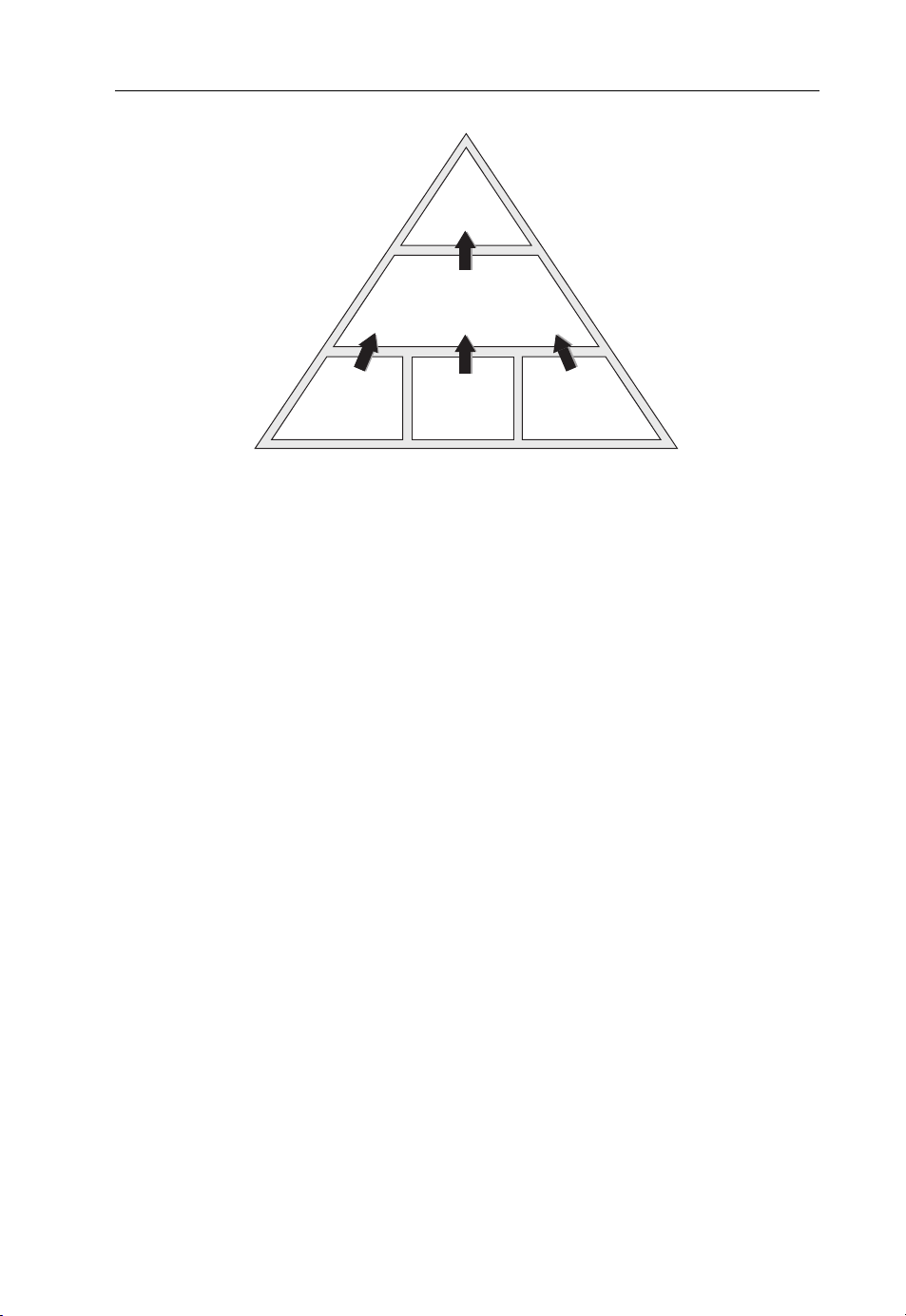
markets as well. Here, the concept of ‘affordability’ comes out in the clearest way. There are
three basic pillars for this which can be illustrated as shown in Figure 1.1.
Liberalization of the whole telecommunications sector – and the resulted regulatory environment – is at least as important an element in overall affordability as any of the technologyderived innovations and business models. This was actually one key element in, for example
Western European mobile success. In most countries the telecom infrastructure was regarded
as a natural monopoly, among other utilities, due to the costs of building and operating the
Page 27
Cellular Technology in Emerging Markets 3
Growth
Affordable
connectivity
Total cost of
ownership
Figure 1.1 The three pillars of telecom development in emerging markets.
Cash barrier
for entry
Regulatory
environment
fixed telephony networks. In many cases it was a government-owned monopoly, and in some
cases partly due to privately and partly government-owned set-ups. With the advent of the first
cellular technologies and mobile telephony services the sector was ready for a drastic change.
The cost dynamics and advantages of cellular technologies made it feasible to open the sector
for competition, overseen by national regulatory bodies. Free competition in a transparent
regulation environment is the best mechanism to really push all technological innovations and
cost break-throughs to the end consumer.
Nothing highlights this better than an example from Nigeria. During the early part of the
2000s Nigeria licensed itsfirst fourmobile operators, three privately ownedand oneincumbent.
In just 18 months the country’s telephony penetration doubled (Trends in Telecommunications
Reform, ITU, 2003). In other words, the mobile operators were able to provide, in 18 months,
as many connections as the government-owned fixed telephony provider from the beginning
of the country’s independence!
Whereas regulatory environment is more of the industry topic in each country the other two
elements of affordability are very much user- or consumer-centric. Cost, or rather the Total
Cost of Ownership (TCO), is the obvious one. The TCO includes all the costs that it takes to
get and stay connected: the cost of the handset, the cost of the subscription and the ongoing
cost of the service itself. All of these typically also include government taxes. Technology
innovations and a massive global scale have greatly reduced the TCO over the last few years.
Another important element is ‘Cash’, that is how do people finance the consumption of the
service. One of the great business model innovations stemming from developing markets is
the pre-paid model where services can be consumed in very small increments – matching the
daily cash situation of particularly low-income segments.
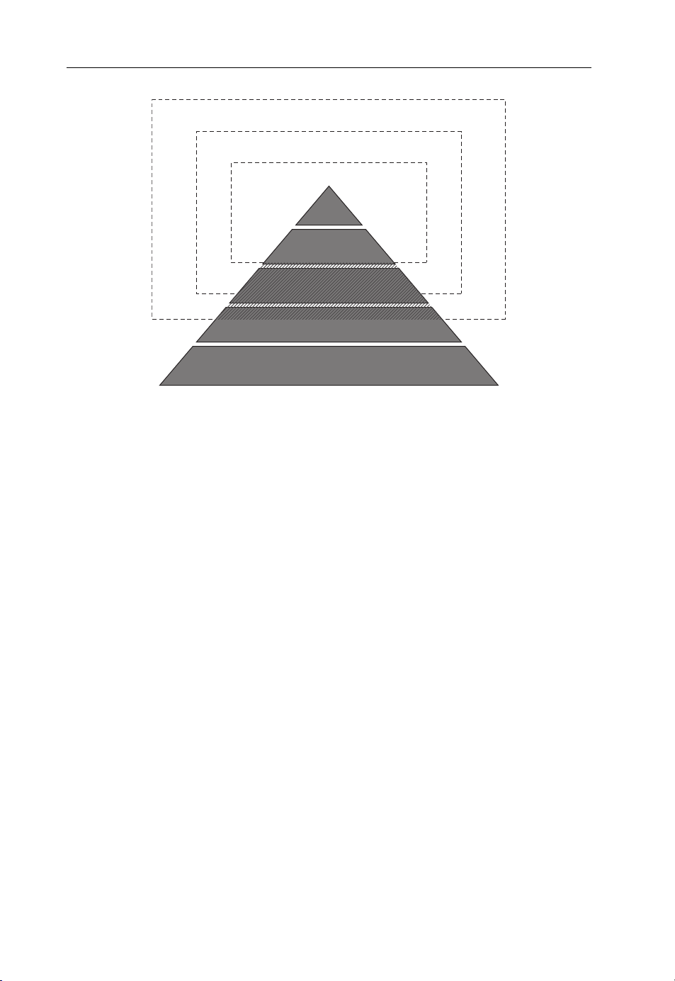
Playing with the two aforementioned aspects – the universal human need to communicate
and the concept of affordability being the main drivers for penetration – it is easy to model
and understand the huge global success of mobile telephony services. Modelling with the
well known ‘income pyramid’ one can readily see that each step downwards in ‘affordability’
brings in a larger potential customer segment (Figure 1.2).
Page 28
4 Cellular Technologies for Emerging Markets
4 billion mobile phone users
3 billion mobile phone users 2008
2 billion mobile phone users 2005
0.8b
>40$/day
1.5b 4-40$/day
1.3b 4$/day
1.4b 2$/day
1.3b 1$/day
Figure 1.2 World population split according to income segment (USD/ capita/day).
The rapiddevelopment ofconnectivity through mobile technologies indeveloping countries
throughout the 2000s was early on identified as one true opportunity to bridge the ‘digital
divide’. In fact, advancing the benefits of ICT technologies was adopted as one of the UN
Millennium Development Goals.
Several international studies have come up with clear evidence between the mobile phone
penetration and macroeconomic development. In a typical emerging market, an increase of
10 mobile phones per 100 people boosts the GDP growth by 0.6 percentage points (Vodafone
policy paper, 2005). A 2006 study byMcKinsey and Company (incooperation withthe GSMA)
found that the indirect impact of mobile phone penetration is at least three times as great. In
addition, the latest study by the World Bank (Quian, 2009) comes up with the figure of a 0.81
percentage GDP boost for low- and middle-income economies.
Lately, the focus of research has been in broadband, instead of pure voice services. The
same World Bank study shows clearly that the 0.81 %-unit boost will increase to 1.12 with
usage of the Internet and all the way up to 1.38 %-units in the case of broadband connectivity
for the services and the Internet.
While the basic mobile connectivity continue to increase beyond the 4B mark it is now
important to have a similar advance in broadband connections. Interestingly, very similar
mechanisms and market behaviour seem to have now taken place in mature markets that led
to the massive increase of mobile voice services 10 years ago. Mobile broadband services
have become affordable – in terms of cost, cash and regulatory environment – so that there
is a ‘fixed-to-mobile’ substitution going on in many markets. The industry has come up with
the necessary technology (speed, latency and end-user devices) and business models (flat rate
pricing) enabling rapid consumer acceptance. Several new services – like social networking –
are once again extending the social dimension to the picture. People want to get into their
services independent of the place and time.
While the technology can’t provide all the answers to unlock the potential of broadband
in developing markets, it surely has a key role as well. The industry knows what it takes to
Page 29
Cellular Technology in Emerging Markets 5
give broadband connectivity a similar success in all parts of the world – and for all people.
Affordability and access, relevant services for people to enhance their business, social or
personal interests will truly make the whole ICT as ‘the biggest democratizer of opportunities
ever seen’.
1.3 Cellular Technologies
Mobile operators usethe radiospectrum to providetheir services. Spectrum is ascarce resource
and has been allocated as such. It has traditionally been shared by a number of industries,
including broadcasting, mobile communications and the military. Before the advent of cellular
technology, the capacity was enhanced through a division of frequencies and the resulting
addition of available channels. However, this reduced the total bandwidth available to each
user, affecting the quality of service. Introduced in the 1970s, cellular technology allowed
for the division of geographical areas (into cells), rather than frequencies, leading to a more
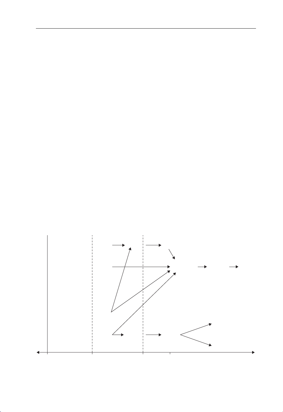
efficient use of the radio spectrum. Figure 1.3 details the evolution of cellular technologies
and the dominant ones at the present time and for the coming years.
Based on usability, cost and quality and quantity of services etc, the evolution of cellular
technology has been divided into generations.
1.3.1 First Generation System
Also referred to as 1G, this period was characterized by analogue telecommunication standards
and supported basic voice services. The development started in the late 1970s with Japan
taking a lead in deployment of the first cellular network in Tokyo, followed by the deployment
1G 2G 3G 4G
GSM
(TDMA)
PDC
(TDMA)
iDEN
(TDMA)
IS-136
AMPS
NMT
1970 1990 2000 2005
(TDMA)
DAMPS
IS-95A
(CDMA)
PDC
GPRS
IS-95B
(CDMA)
EDGE
CDMA
2000
Figure 1.3 Evolution of cellular technology.
UMTS
(WCDMA)
HSDPA
CDMA 2000
(EV-DO)
CDMA 2000
(EV-DV)
LT
E
Page 30

6 Cellular Technologies for Emerging Markets
of NMTs (Nordic Mobile Telephones) in Europe, while the ‘Americas’ deployed AMPS
(Advanced Mobile Phone Service) technology.
Each of these networks implemented their own standards – with features such as roaming
between continents non-existent. This technology also had an inherent limitation in terms of
channels, etc. The handsets in this technology were quite expensive (more than $1000).
1.3.2 Second Generation System
As we have seen above, the various systems were incompatible with each other. Due to this,
work towards development of the next technology was implemented that would lead to a more
harmonized environment. Such work was commissioned by the European Commission and
resulted, in the early-1990s, in the next generation technology known as the ‘Second Generation Mobile Systems’, which were also digital systems as compared to the first generation’s
analogue technology. Key 2G systems in these generations included GSMs (Global Systems
for Mobile Communications), TDMA IS-136, CDMA IS-95, PDC (Personal Digital Cellular)
and PHSs (Personal Handy Phone Systems).
IS 54 and IS 136 (where IS stands for Interim Standard) are the second generation mobile
systems that constitute D-AMPS. IS-136 added a number of features to the original IS54 specification, including text messaging, circuit-switched data (CSD) and an improved
compression protocol. CDMA has many variants in the cellular market. CDMAone (IS-95)
is a second-generation system that offered advantages such as increase in coverage, capacity
(almost 10 times that of AMPS), quality, an improved security system, etc.
GSM was first developed in the 1980s. It was decided to build a digital system based on a
narrowband TDMA solution andhaving a modulation scheme known as GMSK. The technical
fundamentals were ready by 1987 and the first specifications by 1990. By 1991, GSM was the
first commercially operated digital cellular system with Radiolinja in Finland. With features
such as pre-paid calling, international roaming, etc., GSM is by far the most popular and widely
implemented cellular system with more than a billion people using the system (by 2005).
1.3.3 Third Generation System
This improvement in data speed continued and as faster and higher quality networks started
supporting better services like video calling, video streaming, mobile gaming and fast Internet
browsing, it resulted in the introduction of the 3rd generation mobile telecommunication
standard (UMTS). These third generation cellular networks were developed to offer high
speed data and multimedia connectivity to subscribers. Under the initiative IMT-2000, ITU
has defined 3G systems as being capable of supporting high-speed data ranges of 144 kbps to
greater than 2Mbps.
The Universal Mobile Telecommunications System (UMTS) is one of the third-generation
(3G) mobile phone technologies. It uses W-CDMA as the underlying standard. This was
developed by NTT DoCoMo as the air interface for their 3G network FOMA. Later, ITU
accepted W-CDMA as the air-interface technology for UMTS and made it a part of the
IMT-2000 family of 3G standards.
CDMA2000 has variantssuch as 1X,1XEV-DO, 1XEV-DV and 3X.The 1XEV specification
was developedby theThird GenerationPartnership Project2 (3GPP2),a partnershipconsisting
Page 31

Cellular Technology in Emerging Markets 7
of five telecommunications standards bodies: CWTS in China, ARIB and TTC in Japan, TTA
in Korea and TIA in North America.
1.3.4 Fourth Generation System
In the 18th TG-8/1 in 1999, a new working group WP8F was established for looking into the
efforts to develop the systems beyond the IMT-2000. As IMT-2000 was not able to solve the
problems related to higher data rates and capacity, next generation systems (also called as 4G)
development was give that mandate. A 4G system will be a complete replacement for current
networks and be able to provide a comprehensive and secure IP solution where voice, data,
and streamed multimedia can be given to users on an ‘Anytime, Anywhere’ basis, and at much
higher data rates than previous generations. Some features of 4G include the following:
r
The intention of providing high-quality video services leading to data-transfer speeds of
about 100 Mbps.
r
The 4G technology offers transmission speeds of more than 20 Mbps.
r
It will be possible to roam between different networks and different technologies.
r
4G basically resemble a conglomeration of existing technologies and is a convergence of
more than one technology.
1.4 Overview of Some Key Technologies
Let us now have a look at the some of the key technologies.
1.4.1 GSM
GSMs (Global Systems for MobileCommunications) was the first commercially operated digital cellular system. Developed in the 1980s through a pan-European initiative, The European
Telecommunications Standards Institute (ETSI) was responsible for GSM standardization.
Today it is the most popular cellular technology. By mid-2009, GSMs have a user base of
over 3.9 billion in more than 219 countries and territories worldwide; with a market share of
more than 89 % (the global wireless market is more than 4.3 billion). In addition, GSM has the
widest spectral flexibility for any wireless technology – 450, 850, 900, 1800 and 1900 MHz
bands; tri- and quad-band GSM phones are common. Thus it is rare that users will ever travel
to an area without at least one GSM network to which they can connect.
GSM uses TDMA (Time Division Multiple Access) technology and is the legacy network
leading to the third-generation (3G) technologies, the Universal Mobile Telecommunication
System (UMTS) (also known as WCDMA) and High Speed Packet Access (HSPA). GSM
differs from its predecessors in that both signalling and speech channels are digital and thus is
considered a second generation (2G) mobile phone system.
GSM is a very secure network. All communications (voice and data) are encrypted to
prevent eavesdropping. GSM subscribers are identified by their Subscriber Identity Module
(SIM) card. This holds their identity number and authentication key and algorithm. Thus it’s
the card rather than the terminal that enables network access, feature access and billing.
Page 32

8 Cellular Technologies for Emerging Markets
1.4.2 EGPRS
Enhanced GPRS (EGPRS) is another 3G technology that allows improved data transmission
rates. Here EDGE (‘Enhanced Data Rates for GSM Evolution’ – a new radio interface technology with enhanced modulation) is introduced on top of the GPRS and is used to transfer
data in a packet-switched mode on several time slots, as an extension on top of the standard
GSM. This leads to almost an increase in data rates of almost three-fold.
The major advantage of EDGE is that it does not require any hardware or software changes
in the GSM core networks. No new spectrum is required and thus EDGE can effectively be
launched under the existing GSM license. WCDMA (including HSPA) and EDGEsystems are
complimentary. There is a wide range of EDGE capable user devices in the market, including
USB modems, modules for PCs, phones, routers, etc.
EDGE was first deployed by Cingular (now AT&T) in the United States in 2003. By mid2009 there were more than 440 GSM/EDGE networks in 181 countries, from a total of 478
mobile network operator commitments in 184 countries.
1.4.3 UMTS
The Universal Mobile Telecommunications System (UMTS) is a voice and high-speed
data technology that is ‘part’ third-generation (3G) wireless standards. Wideband CDMA
(WCDMA) is the radio technology used in UMTS. Furthermore, UMTS borrows and builds
upon concepts from GSM and most UMTS handsets also support GSM, allowing seamless
dual-mode operation.Therefore, UMTSis also marketed as 3GSM. UMTS is based onInternet
Protocol (IP) technology with user-achievable peak data rates of 350 kbps.
UMTS builds on GSM and its main benefits include high spectral efficiency for voice
and data, simultaneous voice and data for users, high user densities supportable with low
infrastructure costs, high-bandwidth data applications support and migration path to VoIP in
future. Operators can also use their entire available spectrum for both voice and high-speed
data services.
UMTS has been in commercial usage since 2001, in Japan. As of April 2009, it was available
with 282 operators in more than 123 countries and enjoyed a subscriber base of 330 million.
As for GSM, UMTS can also work over a wide range of spectrum bands – 850, 900, 1700,
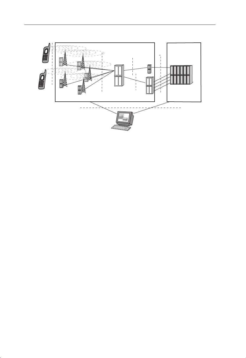
1800, 1900, 2100and 2600 MHz bands(450 MHz and 700MHz areexpectedto beadded soon).
Thus transparent global roaming is an important aspect of UMTS. Also, UMTS operators
can use a common core network that supports multiple radio-access networks, including
GSM, EDGE, WCDMA, HSPA, etc. This is called the UMTS multi-radio network (shown in
Figure 1.4) and provides great flexibility to operators.
UMTS networks can be upgraded with High-Speed Downlink Packet Access (HSDPA),
sometimes known as 3.5G. Currently, HSDPA enables downlink transfer speeds of up to
21 Mbs.
1.4.4 CDMA
Code Division Multiple Access (CDMA) was originally known as IS-95. It is the major
competing technology to GSM. There are now different variations, but the original CDMA is
now known as cdmaOne.
Page 33

Cellular Technology in Emerging Markets 9
Circuit
GSM
EDGE
Switched
Networks
WCDMA,
HSDPA
WLAN etc
UMTS
Core Network
External NetworksRadio Access Networks
Figure 1.4 UTMS multiradio network.
Packet
Switched
Networks
Other
Cellular
Operators
Currently there is cdma2000 and its variants like 1X EV, 1XEV-DO and MC 3X. The
technology is used in ultra-high-frequency (UHF) cellular telephone systems in the 800-MHz
and 1.9-GHz bands. CDMA employs spread-spectrum technology along with a special coding
scheme and is characterized by high capacity and a small cell radius.
CDMA was originally developed by Qualcomm and enhanced by Ericsson. However,
QUALCOMM still owns a substantial portfolio of CDMA patents, including many patents
that are necessary for the deployment of any proposed 3G CDMA system. It has now been
granted royalty-bearing licenses to more than 75 manufacturers for CDMA and, as part of
these licenses, has transferred technology and ‘know-how’ in assisting these companies to
develop and deploy CDMA products.
CDMA was adopted by the Telecommunications Industry Association (TIA) in 1993. In
September 1998, only three years after the first commercial deployment, there were 16 million
subscribers on cdmaOne systems worldwide. By mid-2009, there were around 500 million
subscribers on CDMA (including variants).
Another variant of CDMA is TDS-CDMA. Time Division Synchronous Code Division
Multiple Access (TD-SCDMA) or UTRA/UMTS-TDD, also known as UMTS-TDD or IMT
2000 Time-Division, is an alternative to W-CDMA. Although the name gives an impression of
simply a channel access method based on CDMA, its applicability is to the whole-air interface
specification.
The technology is promoted by the China Wireless Telecommunication Standards group
(CWTS) and was approved by the ITU in 1999. It is being developed by the Chinese Academy
of Telecommunications Technology, Datang, and Siemens AG, and is China’s country’s standard of 3G mobile telecommunication. However, it is expected to remain as a niche market
technology as it lacks a large ecosystem and would muster limited research and development.
In addition, necessary competition and economies of scale to reduce investments and generate
demand might be missing, besides the fact that its delayed arrival has given rival 3G technologies a good head start. TD-SCDMA came under spotlight as one of the technologies used in
the 2008 Olympics at Beijing, China.
1.4.5 HSPA
High Speed Packet Access (HSPA) is a collection of two mobile telephony protocols, namely
High Speed Downlink Packet Access (HSDPA) and High Speed Uplink Packet Access
Page 34

10 Cellular Technologies for Emerging Markets
(HSUPA). It is basically an extension/improvement of the performance of existing WCDMA
protocols. HSPA improves the end-user experience by increasing peak data rates up to
14 Mbps in the downlink and 5.8 Mbps in the uplink, according to network and user
device capabilities.
Mobile broadband is a key part of the commercial offering of most mobile network operators
today and the strong market uptake which has been seen in every market is boosting revenues
and profits. The path to mobile broadband began with WCDMA and has grown globally with
HSPA to boost capacity and user data speeds. Several operators have positioned HSPA as an
alternative to fixed broadband, with the added value of mobility.
HSPA has been commercially deployed by over 270 operators in more than 110 countries,
as of 2009. Data traffic and revenues are growing strongly with HSPA. According to GSA
surveys of the mobile broadband market, WCDMA has a 72 % market share of commercial
3G networks. More than 90 % of the 275 commercial WCDMA network operators have
launched HSPA.
1.4.6 LTE
LTE (Long Term Evolution) is marked as the 4th generation of mobile technology designed
to provide uplink peak rates of at least 50Mbps and downlink peak rates of at least 100 Mbps.
The specifications support both Frequency Division Duplexing and Time Division Duplexing.
Designed as a flat IP-based network architecture it can replace the GPRS Core Network and
ensure support for, and mobility between, some legacy or non-3GPP systems such as GPRS
and WiMax.
LTE has been designed to offer ‘rich’ broadband user experience and will further enhance
mobile value-added services and applications supporting banking, gaming, health categories,
etc. Even experience with more demanding applications such as interactive TV, mobile video
blogging, advanced games, etc will also be significantly improved.
The main advantages with LTE are high throughput, low latency, ‘plug-and-play’, besides
improved end-user experience and simple architecture resulting in low-operating expenditures.
LTE will also support seamless integration with older network technologies, such as GSM,
CDMA, UMTS and CDMA2000. LTE is the natural migration choice for GSM/HSPA operators. LTE is also the next generation mobile broadband system of choice of leading CDMA
operators, who are expected to be in the forefront of service introduction.
With over 39 LTE commitments in 19 countries, at least 14 networks are expected to be
commercially deployed by 2010. It is expected that there will be nearly 34 million users
worldwide by 2010 that are expected to reach 400–450 million users by 2015. Some of the
first operators intending to deploy LTE include Verizon Wireless, MetroPCS Wireless and US
Cellular in the United States, NTT-DOCOMO and KDDI in Japan, TeliaSonera, Tele2 and
Telenor in Europe, China Mobile in China, and KT and SK Telecom in Korea, in 2010.
1.4.7 OFDM
OFDM (Orthogonal Frequencies DivisionMultiplexing) is a broadband technique like CDMA.
In this, instead of modulating a single carrier as is the case with FM or AM, a number of carriers
are spread regularly over a frequency band. Orthogonal FDMs (OFDM) spread-spectrum
Page 35

Cellular Technology in Emerging Markets 11
techniques distribute the data over a large number of carriers that are spaced apart at precise
frequencies. This spacing provides the ‘orthogonality’ in this technique which prevents the
demodulators from seeing frequencies other than their own.
OFDM has been successfully used in DAB and DVB systems. For DAB, OFDM forms the
basis for the Digital Audio Broadcasting (DAB) standard in the European market. For ADSL,
OFDM forms the basis for the global ADSL (Asymmetric Digital Subscriber Line) standard.
For Wireless Local Area Networks, development is ongoing for wireless point-to-point and
point-to-multipoint configurations using OFDM technology. In a supplement to the IEEE
802.11 standard, the IEEE 802.11 Working Group published IEEE 802.11a (details of these
standards are described later in Chapter 7 of this book) which outlines the use of OFDM in
the 5.8 GHz band. This technology is starting to play an important role in development of
fourth-generation networks.
1.4.8 All IP Networks
NGNs (Next-Generation Networks) are ‘packet-based’ networks, based upon Internet Protocol. Complementary to LTE, another project under development at 3GPP is SAE (System
Architecture Evolution). While LTE aims at an evolved radio access network, SAE deals with
core network, with a focus on packet domain. Thus the developments of the 3GPP system are
compliant with Internet protocols. It is an evolution of the 3GPP system to meet the growing
demands of the mobile telecommunications market and is designed to make use of multiple
broadband technologies and other ‘Quality of Service’-enabled transport technologies where
service-related functionsare independent from underlying transport-relatedtechnologies. This
will ensure generalized mobility which will allow consistent and ubiquitous provision of services to users, besides the capability to deliver telephony, television, data and a host of other
services at lower marginal cost then the current networks. In 2004, 3GPP proposed IP as the
future for next-generationnetworks and began feasibilitystudies into AllIP Networks (AIPNs).
1.4.9 Broadband Wireless Access
Broadband wireless technologies have opened up possibilities of high-speed, affordable Internet access anywhere and at any time. Although this technology has been available for quite
some time, however, ‘islands’ of proprietary deployment has significantly increased the cost
of service and hindered its global expansion. Around about 2003, broadband wireless began
to emerge as the key to resolving connectivity bottlenecks. A typical BWA spectrum in shown
in Figure 1.5.
Several governments started appreciating the importance of broadband connectivity for
social, economic and educational development. They started initiatives to support sustainable
broadband services in various regions. Meanwhile, standardization bodies such as IEEE and
ITU also started work towards standardizationof technologies and harmonization of regulatory
frameworks worldwide.
Some key technologies that fall under BWA are described in the following sections.
1.4.9.1 WiMAX
WiMAX stands for ‘Worldwide Interoperability for Microwave Access’. It was developed
by the WiMAX Forum; formed in June 2001 to promote conformity and interoperability of
Page 36

12 Cellular Technologies for Emerging Markets
700
MHz
902-928
Licensed
Unlicensed
Lightly Licensed
2.1
MHz
GHz
Figure 1.5 Broadband wireless spectrum.
2.3
GHz
2.4
GHz
2.5-
MHz
2.7
3.3-
3.8
GHz
4.9
GHz
5.8
GHz
the standard. WiMax was designed as an alternative to cable and DSL, to enable the ‘lastmile delivery’ of wireless broadband access and has been considered as a wireless ‘backhaul
technology’ for 2G, 3G and 4G networks. However, it is also a possible replacement candidate
for other telecommunication technologies such as GSM and CDMA, and can also be used as
an overlay to increase capacity.
WiMAX’s main competition comes from existing and widely deployed wireless systems
such as UMTS and CDMA2000. Also, 3G/LTE technologies are being touted as ‘WiMax
killers’. By 2008, WiMax had a subscriber base of more than 2.5 million with 450 WiMAX
networks deployed in over 130 countries.
1.4.9.2 Wi-Fi
Wi-Fi stands for ‘Wireless Fidelity’. With Wi-Fi, it is possible to create high-speed wireless
local area networks, provided that the computer to be connected is not too far from the access
point. Inpractice, Wi-Fi canbe used to provide high-speed connections(11 Mbps or greater) to
laptop computers,desktop computers, personal digital assistants (PDAs) and any other devices
located within a radius of several dozen metres indoors (in general, 20–50 m away) or within
several hundred metres outdoors.
1.4.9.3 Wireless LAN
WLAN (Wireless Local Area Network) is commonly known as Wireless LAN. Generally it
is understood as being the technology which links two or more computers or devices without
using wires. WLAN uses spread-spectrum or OFDM modulation technology based on radio
wavesto enablecommunication between devicesin a limited area. InWLAN, usersget the ability to be connected to a network whilestill beable tomove around within a broadcoverage area.
1.4.10 IMS
The IP Multimedia Subsystem (IMS) is an IP-based architectural framework for delivering
voice and multimedia services. The specifications have been defined by the 3rd Generation
Partnership Project (3GPP). This is based on the IETF Internet protocols and is ‘accessindependent’. It supports IP to IP sessions over 802.11, 802.15, wireline, CDMA, GSM,
EGPRS, UMTS and other packet data applications.
Page 37

Cellular Technology in Emerging Markets 13
IMS intends to make Internet technologies, such as web browsing, instant messaging,
e-mail, etc, in addition to services such as WAP and MMS, ubiquitous. IMS is expected to
lead to new business models and opportunities.
IMS has given the operators and service providers with the power to control and charge
for the services they have provided. Some of the key services involve multi-media messaging
services (MMSs), ‘Push-to-talk’, etc. There are ‘Capex’ and ‘Opex’ savings when using the
converged IP backbone and open IMS architectures. There are also some hidden advantages
such as usage of standardized interfaces which would prevent operators from being ‘bounded’
by single supplier’s proprietary interfaces and the existing infrastructure can be used to create
new services.
1.4.11 UMA
Unlicensed Mobile Access (UMA) is the commercial name of the 3GPP Generic Access
Network (GAN) standard. This technology provides access to GSM and GPRS mobile services
over unlicensed wireless networks such as Bluetooth and 802.11.
This technology enables its users to roam and handover between cellular networks and
wireless LANs/WANs using dual-mode (GSM/Wi-Fi) mobile handsets, ensuring a consistent
user experience for their mobile voice and data services. This is akin to convergence between
mobile, fixed line and Internet telephony.
The fundamental idea behind UMA was to provide a high bandwidth and low-cost wireless
access network integrated into operator cellular network. Features such as seamless continuity
and roaming were a part of this. This led to development of the UMAC (Unlicensed Mobile
Access Consortium0 that promoted the UMA technology. UMAC worked with the 3GPP and
the first set of specifications appeared in 2004. 3GPP was defined by the UMA as a part of the
‘3GPP Release 6’ (3GPP TS 43.318) under the name of GAN (Generic Access Network)
1.4.12 DVB-H
Digital Video Broadcasting (DVB) is a suite of internationally accepted open standards for
digital television. This standard is led by a consortium of over 270broadcasters, manufacturers,
network operators, software developers, regulatory bodies and others in over 35 countries. It
is intended as an open technical standard for the global delivery of digital television and data
services. Services on this standard are currently available on every continent with more than
220 million DVB receivers deployed.
The concept of providing television on handheld devices led to the development of DVB
technology for handheld or DVB-H. The Digital Video Broadcast (DVB) Project started
research workrelated tomobile receptionof DVB-Terrestrial (DVB-T)signals as early as1998,
accompanying the introduction of commercial terrestrial digital TV services in Europe. The
EU sponsored projects, such as ‘Motivate’ and the ‘Media Car platform’ came up with various
conclusions, for example transmissions possible on DVB-T networks, but more robustness
needed and the addition of spatial diversity increases the reception performance which helped
in the development of mobile TVs. In the year 2002, work started in the DVB Project to define
a set of commercial requirements for a system supporting handheld devices. The technical
work then led to a system called Digital Video Broadcasting-Handheld (DVB-H), which was
Page 38

14 Cellular Technologies for Emerging Markets
published as a European Telecommunications Standards Institute (ETSI) Standard EN 302
304 in November 2004.
1.5 Future Direction
Radio technology and standards are still very much in an active development phase. Researchers are continuously coming up with advancements for optimally using the spectrum
and in ways which are cost-efficient as well. Complex signals processing mathematics are
employed to reconstruct a data stream from an encoded radio wave. With processing powers
becoming cheaper, more complex algorithms can be used to improve performance. While
there are theoretical limits to such improvements, it is still a long way off.
Similarly,work isongoing toprovide betteruser experience,for exampleif thesame handset
can work with multiple standards then it can be used as an extension within small premises
and used as an handset when the person leaves the building.
Thus it is certain that in the coming years, radio technology will become more digital and
smarter. It is then up to regulators and technologists as to how this advancement will be
encapsulated within the existing and future regulatory and deployment frameworks.
Page 39

2
GSM and EGPRS
2.1 Introduction
The limitations ofthe firstgeneration analogue mobile telephonysystem ledto the development
of the second generation mobile systems. Systems such as Nordic Mobile Telephones (NMT)
in (Scandinavian) Europe, AMPS (Advanced Mobile Phone Service) in the USA and TACS
(Total Access Communication System) in the UK operated under the so-called first generation
systems. However, they were incompatible with each other and covered a small geographic
area. Though developments did take place within these systems, however, digital revolution
paved the way for the next wave of mobile systems which went on to cover most of the planet.
These second generation digital systems were more harmonized and of course had a digital
technology at their foundation leading to better voice quality and spectrum utilization. Many
variants of second generation systems came in different markets that included GSM (Global
Systems for Mobile Communications), TDMA IS-136, CDMA IS-95, PDC (Personal Digital
Cellular) and PHS (Personal Handy Phone System). However, in this chapter, we will only
discuss in detail the GSM and EGPRS systems.
The GSM system is the most popular second generation technology with over a billion
people connected through this system (in 2007, the world saw more than 3 billion people
connected to voice telephony). The first GSM networks appeared up commercially in the
early 1990s but, however, work on these systems started as early as during the 1980s. Based
on the GSMK modulations scheme, GSM was a TDMA solution. With the specification
ready by 1991, the stage was set for the first commercial networks. The popularity of this
system, along with smaller handsets invading the market, boosted the mobile subscriber
figures. The short messaging system (SMS) became a ‘killer application’, the popularity of
which can be gauged by the fact that an estimated number of more than a trillion short
messages were sent across the world in 2008 (almost 15 billion SMSs were sent in the year
2000 alone).
With data ‘knocking on the doors’ of the mobile world an extension to GSM networks in the
form of GPRS (General Packet Radio Service) came into being. In simpler terms, to the already
existing network the form of packet core was added to handle the data traffic. The theoretical
speed of these networks was up to 171.2 kilo bits per second (kbps). An enhancement to the
data speeds led to enhancements in GPRS networks and were known as EGPRS networks. We
Cellular Technologies for Emerging Markets: 2G, 3G and Beyond Ajay R. Mishra
C
2010 John Wiley & Sons, Ltd
Page 40
16 Cellular Technologies for Emerging Markets
Air
BSS
Abis
BTS
Figure 2.1 GSM architecture.
BSC
Ater’
Ater
TC
TCSM
NMS
NSS
A
MSC
will discuss later the architecture of these networks and the reasons that led to greater data
speeds.
2.2 GSM Technology
2.2.1 GSM Network
Let us understand the key components of the GSM network. The latter consists of three
main domains: the Mobile Station (MS), the Base Station Sub-system (BSS), the Network
Sub-system (NSS) and the Network Management System (NMS), as shown in Figure 2.1.
2.2.1.1 Mobile Station (MS)
The mobile station is perhaps the most important part of the whole system. Why is this?
Simply because the subscriber uses this to talk. Plus the whole network quality could be well
perceived by the subscriber based on the experience of using/talking on his/her mobile. There
are various mobile devices available on the market, possibly with all possible permutation and
combinations of voice, data, music, cameras, etc., ranging from a few dollars to thousands of
dollars. However, let us try to understand what are the ‘blocks’ that make up a simple GSM
mobile station. An MS is made up of two main parts, as shown in Figure 2.2: the handset
itself and the subscriber identity module (SIM). The latter is personalized and is unique to the
subscriber. The handset or the terminal equipment should have qualities similar to that of fixed
phones in terms of quality, apart from being ‘user-friendly’ in usage. It also has functionalities
such as GMSK modulation and demodulation up to channel coding/decoding. Plus it needs to
possess dual tone multi-frequency generation and should have a long lasting battery.
The SIM or SIM card is basically a microchip operating in conjunction with the memory
card. The SIM card’s major function is to store the data for both the operator and subscriber.
The SIM card fulfills the needs of the operator and the subscriber as the operator is able to
Page 41

GSM and EGPRS 17
Voice
Encoding/
Decoding
Channel
Encoding/
Decoding
Ciphering/
De-ciphering
SIM card
Mod. + Amp./
Demodulation
Figure 2.2 Block diagram of the GSM mobile station.
maintain control over the subscription and the subscriber can protect his personal information.
Thus, the most important SIM functions include authentication, radio transmission security
and storing the subscriber data.
2.2.1.2 Base Station Sub-system (BSS)
The BSS consists of the base transceiver station (BTS), base station controller (BSC) and
trans-coder sub-multiplexer (TCSM). The TCSM is usually physically located at the MSC.
Base Transceiver Station (BTS)
The BTS is the interface between the BSC and the mobile station (or subscriber). Due to
its position in the network, that is connecting the subscriber’s mobile system to the network,
this becomes an important element. As the name suggests, the BTS contains elements called
‘transceivers’ that have the capability to transmit and receive. These transceivers (or TRXs)
are connected to the antennae through which information is transmitted/received to/from the
mobile station, as shown in Figure 2.3. The antennae can be omni-directional or directional
ones. The base stations usually have one to three sectors. Each sector is usually located at 120
degrees (the actual angle is dependent upon radio network plans), thus covering a 360 degree
area around them. Each sector antenna is connected to the TRXs in the BTS, while the number
Air
interface
Filter
Output/Input
TRX
O&M
Transmission
System
Figure 2.3 A BTS with sector antennas and the corresponding block diagram.
Abis
interface
Page 42

18 Cellular Technologies for Emerging Markets
of TRXs’ are dependent upon the subscribers that are needed to be catered in that particular
direction.
The BTS maintains synchronization to the mobile station. It also consists of a transmission
unit, known as the TRU. This is the unit that interacts with the various interfaces, such as
and A
A
bis
, and which is responsible for allocating the traffic and associated signalling to
ter
the correct TRX. Cross-connections are possible at the 2 Mbps level and have a ‘drop-insert
facility’ at the 8 kbps level. Other functions include providing radio interface timing, detecting
the access attempts of the mobile station, performing the frequency hopping function and
RF signal processing functions such as combining, filtering, coupling etc., encryptions and
de-encryption on the radio path, channel coding and decoding, interleaving on the radio path
and forwarding the measurement data to the BSC based on which it (BSC) makes decisions
related to the mobile station.
Base Station Controller (BSC)
As the name suggest, the BSC controls the base transceivers stations in a network. One
BSC controls several BTSs in a network. In simpler terms, the BSC can also be called the
‘brain’ of the network. This can be well understood by the kind of functions that a BSC
handles. As mentioned above, the BTS sends the measurements data to the BSC, based
on which the BSC makes the decisions related to the mobile stations, that is the BSC is
responsible for radio resource management and configuration. These include functions such
as BCF, BTS, TRX management and channel allocation,channel release,radio linksupervision
(measurement handling) and powercontrol (BTS and MS). Towhich cella ‘moving subscriber’
needs to be connected, the BSC decides on this, based on the measurement reports from
the BTS. This decision is based on inputs such as signal quality, signal level, interference,
power budget calculations and distance. To improve the link quality between the BTS and
MS, frequency hopping management is carried out by the BSC (including implementing
no-frequency hopping’, baseband-frequency hopping and synthesized frequency hopping).
The BSC is also responsible for signalling between the BSC-MSC (CCS7) and the BSCBTS (LAPD, TRXSIG, BCFSIG). Encryption management functions, such as storing the
encryption parameters and forwarding them to the BTS, are conducted by the BSC. A block
diagram of a typical BSC is shown in Figure 2.4. The switch matrix (SM) takes care of the
relay functions and the inter-working of the A
and A interface signals coming from the
bis
BTS an BSC. Connections to the BTS are established through the Terminal Control Elements
(TCEs) which also provides the control functions. On the A interface side as well, the TCE
provide similar functions. The database maintains the status of the whole BSS, including the
BTS operations and BSS information such as frequency, quality, etc. The central functions are
responsible for tasks such as handover decisions, power control, etc.
Transcoder and Sub-Multiplexer (TCSM)
Although the TCSM is physically located at the MSC it is controlled by the BSC and hence it
is a part of the BSS. Therefore, planning for this is a part of a transmission planning engineer’s
job description. The transcoder converts the 64 kbps signal to 16 kbps. It converts the 160
A-law PCM samples of an 8-bit speech channel (20 ms) into a ‘vocoder block’. This creates
a TRAU frame that is assigned on the PCM signal towards the A-interface direction. In the
downlink direction, the TC also performs the speech activity function wherein if no speech
Page 43

GSM and EGPRS 19
DB
TM/TCE
TCE/TM
TM/TCE
TM/TCE
SW
Central Functions
TCE/TM
TCE/TM
Figure 2.4 Block diagram of the BSC.
is detected then the comfort background noises are transmitted to the mobile station. The
sub-multiplexer rearranges the 16 kbps signals more effectively, thus increasing the possibility
of reducing the number of 2 Mbps links on the A
interface (typically by a factor of 3 to 4) –
ter
see Figure 2.5.
2.2.1.3 Network Sub-System (NSS)
The network sub-system acts as an interface between the GSM network and the public networks, PSTN/ISDN. Themain components ofthe NSSare theMSC, HLR, VLR,AUCand EIR.
Mobile Switching Centre (MSC)
The MSC or ‘Switch’ as it is generally called, is the single most important element of the
NSS as it is responsible for the switching functions that are necessary for the inter-connection
between the mobile users and that of the mobile and the fixed network users. For this purpose,
BSC
TC
TC
SM
TC
TC
Figure 2.5 Transcoder and sub-multiplexer.
MSC
Page 44

20 Cellular Technologies for Emerging Markets
CCSU
BSU
CCMU
CASU
PAU
LSU
ICWU BDCU ECU ET
Figure 2.6 Block diagram of the MSC/VLR.
SW
TGFP
CNFC
VLRU
CMU
STU
CHU
the MSC makes use of the three major components of the NSS, that is the HLR, VLR and
AUC. A block diagram of the MSC is shown in Figure 2.6.
CCSU (Common Channel Signalling Unit)
This handles trunk signalling (SS7) towards the HLR, other MSCs and PSTN exchanges.
BSU (Base Station Signalling Unit)
This handles SS7 signalling towards the BSC and call control for mobile-originated calls.
CCMU (Common Channel Signalling Management Unit)
This handles the centralized functions of the SS7 signalling system (needed in large exchanges
while in smaller exchanges the CCMU functions are carried out by the CM and STU).
CASU (Channel Associated Signalling Unit)
This performs R2 signalling.
PAU (Primary Access Unit)
This handles DPNSS signalling towards the PABXs.
LSU (Line Signalling Unit)
This controls the announcement machine (ANM).
IWCU (Inter-Working Control Unit)
This controls the Compact Data Services Unit (CDSU) and Echo Cancellers (ECs).
Page 45

GSM and EGPRS 21
GSW (Group Switch)
This performs the basic function of the MSC which is switching of telephone calls.
TG (Tone Generator)
This is responsible for generating various types of tones such as dial tone, busy tone, information tone, etc.
DTMFG (Dual Tone Multi-Frequency Generator)
This is used for generating DTMF signals.
CNFC (Conference Circuit)
This is used for enabling multi-party conferences.
VLRU (Visitor Location Register Unit)
This performs the VLR functions.
CMU (Cellular Management Unit)
As the name suggests, this controls and supervises the cellular network and handovers.
CHU (Charging Unit)
This collects the charging data.
STS (Statistical Unit)
This collects the exchange-specific statistical data.
OMU (Operation and Maintenance Unit)
This performs the operation and maintenance tasks.
BDCU (Basic Data Communications Unit)
This contains all communication links to O and M networks (terminals for X.25 packet
networks and/or for the time slots of PCM links) and to the ‘Billing Centre’.
ECU (Echo Canceller Unit)
This is needed in interworking to the PSTN.
ET (Exchange Terminal)
This is the unit which handles the external 2 Mb PCM circuits.
Home Location Register (HLR)
The HLR contains the information related to each mobile subscriber. Each subscriber mobile
has some information that contains data such as the kind of subscription, services that the user
can use, the subscriber’s current location and the mobile equipment status. The database in the
HLR remains intact and unchanged until the validity of the subscription.
Page 46

22 Cellular Technologies for Emerging Markets
Visitor Location Register (VLR)
The VLR(Visitor Location Register) comes into actiononce the subscriber enters the coverage
region. Unlike the HLR, the VLR is ‘dynamic’ in nature and interacts with the HLR when
recoding the data of a particular mobile subscriber. When the subscriber moves to another
region, the database of the subscriber is also shifted to the VLR of the new region.
Authentication Centre (AUC)
The Authentication Centre (AUC or AC) is the ‘responsibility’ for the policing actions in the
network. This has all the data that is required to protect the network against false subscribers
and protection of the calls of the regular subscribers. There are two major keys in the GSM
standards, for example one which is the encryption of the mobile users and the other which is
‘authentication’ of the mobile users. The encryption keysare heldboth inthe mobileequipment
and the AUC and the information is protected against non-authorized access.
Equipment Identity Registers (EIRs)
Each item of mobile equipment has its own personal identification, which is denoted by
a number known as the International Mobile Equipment Identity (IMEI). This number is
installed during the manufacture of the equipment itself, stating the conformation to the GSM
standards. Thus, whenever a call is made, the network would check the identity number and if
this number is not found on the approved list of the authorized equipment, the access is denied.
The EIR contains this list of the authorized numbers and allows the IMEI to be verified.
2.2.1.4 Network Management System (NMS)
The main task of the network management system is to ensure that the running of the network
is smooth. For this purpose, it has four major tasks to perform: network monitoring, network
development, network measurements and fault management. Once the network is up and
running, the NMS takes over the responsibility to monitor the performance of the network.
If it sees some faults, it would generate relevant alarms. Some of the faults may be corrected
through the NMS itself (mostly software-oriented) while for some sites, visits would be
required. The NMS is also responsible for the collection of data and analyses its performance,
thereby leading to accurate decisions related to the optimization of the network. The capacity
and the configuration of the NMS are dependent upon the size (both in terms of capacity and
geographical area) and the technological needs of the network.
2.2.2 Signalling and Interfaces in the GSM Network
Let’s start from the MSC to the MS. Signalling between the MSC and BSC is the CCS#7
and is transferred using 64 kpbs timeslots. It passes through the transcoder but the submultiplexer arranges the signalling channel from multiple A interface PCM frames to the end
of the Ater interface PCM. LAPD signalling is used between the BSC and BTS. These are
of two types: TRXSIG and OMUSIG. Some information coming from the BSC in TRXSIG
is transferred to the MS using the LAPDm protocol in the air-interface. The TRXSIG is used
for performing functions such as call control, both the uplink and downlink measurements,
Page 47

GSM and EGPRS 23
paging, handover, etc., while the OMUSIG is used for downloading of the BTS software from
the BSC, monitoring and control purposes.
2.2.2.1 Air-Interface
The interface between the MS and BTS is the air-interface. The speech signal generated by the
MS is encoded by the A or the µ law to 8-bit samples at a 8 kHz sampling rate. This speech
is coded in the transcoder of the GSM system to bring the rate from 64 kbps to an effective
bit rate of 13 kbps. Some additional coding is required for protecting the signal against noise
and distortion and this requires an additional (approximately) 3 kpbs, thus making a total in
all of 16 kbps (traffic plus signalling). These traffic signals are allocated on the TDMA frame,
having 8 TS. With a TS of 0 being used for signalling such as PCH, RACH, etc., the remaining
seven are used to carry the traffic. As mentioned before, LADm is used between the MS and
BTS.
2.2.2.2 Abis-Interface
The Abis-interface exists between the BTS and BSC. Usually, 16 kbps signalling is used on
this interface. The number of the TRXs supported by this interface depends upon the type of
signalling. The higher the signalling, the lower the amount of TRX it would be able to support.
The traffic channels are 16 kbps. Usually, 96 traffic channels per 2 Mbps are supported with
one TRXSIG per TRX and one OMUSIG per BTS on the Abis-interface.
2.2.2.3 Ater-Interface
The interface between the BSC and TCSM is the Ater-interface. The traffic and signalling
channels coming from the PCMs from the MSC are re-allocated in the TCSM. The ‘Ater’
contains 16 kbps traffic channels. Each 2 Mpbs contains up to 116 (or 120) traffic channels. It
contains 64 kbps CCS#7 signalling channels and 64 kbps channel for X.25.
2.2.2.4 A-Interface
The A-interface exists between the MSC and TCSM. It contains 30 and 64 kbps traffic channels
within each 2 Mbps frame. Also present is 64 kbps CCS#7 signalling and X.25. A TS16 in the
A-interface is generally used for CCS#7 signalling purposes.
These interfaces are shown in Figure 2.7.
2.2.3 Channel Structure in the GSM
The frequency spectrum for GSM systems is limited. It combines both the TDMA and FDMA
techniques for ‘best use’ of the frequency bands. The frequency bands of 890–915 MHz
for downlink and 935–960 MHz for uplink are used for the GSM system. Both of these
are divided into 124 carrier frequencies of 200 kHz each. The time division of each carrier
frequency creates ‘time slots’, each numbered from 0 to 7. One burst in the TDMA frame
Page 48

24 Cellular Technologies for Emerging Markets
Air
A
bis
BTS
Figure 2.7 Air-, A
BSC
A
’
ter
A
ter
-, A
- and A-interfaces.
bis
ter
TCSM
A
TC
MSC
equals one time slot which equals one logical channel. There are two types of channels:
physical and logical channels. The formers onesare actual time slots between the BSS and MS
while the latter ones are needed for structuring and signalling purposes. The physical channels
are of two types: Half-Rate (HR) and Full-Rate (FR). While the FR channel is a 13 kbps coded
speech or data channel with a raw data rate of 9.6, 4.8 and 2.6 kbps, the HR supports 7, 4.8
and 2.4 kbps. The logical channels are also of two types: Traffic Channels (TCHs) and Control
Channels (CCHs).
The bit rates of the traffic channels (TCHs) can be 13 kbps (FR), 5.6 kbps(HR) or an
Enhanced Full Rate (EFR) of 12.2 kbps. The EFR is a dedicated channel for one user. AMR
(Adapative Multirate Coding) is another codec type that allows the adaptation of source and
channel coding according to network conditions, thus resulting in better quality and capacity
savings.
Logical control channels are basically of two types: Common Control Channels (CCCHs)
and Dedicated Control Channels (DCHs). Table 2.1 summarizes the logical control channels
in a GSM network along with their function.
Table 2.1 Logical control channels in GSM
Channel Abbreviation Function/Application
Access Grant Channel (DL) AGCH Resource allocation, that is subscriber
access authorization
Broadcast Common Control Channel
BCCH Dissemination of general information
(DL)
Cell Broadcast Channel (DL) CBCH Transmits the cell broadcast messages
Fast Associated Control Channel FACCH For user network signalling
Paging Channel (DL) PCH Paging for a mobile terminal
Random Access Channel (DL) RACH Resource request made by mobile terminal
Slow Associated Control Channel SACCH Used for transport of radio layer parameters
Standalone Dedicated Control Channel SDCCH For user network signalling
Synchronization Channel (DL) SCH Synchronization of mobile terminal
Page 49

GSM and EGPRS 25
Network
Customer
Inputs
Dimensioning
Nominal
Planning
Optimization
Cycle
Parameter
Tuning
Parameter
Planning
Figure 2.8 Network planning and optimization process.
Detailed
Planning
2.3 Network Planning in the GSM Network
2.3.1 Network Planning Process
As shown in Figure 2.8, the network planning process starts with the customer/network
operator. The ‘operator’ is the one who decides on the fundamental specifications/outlines of
the network and gives this information to the vendor who is able to deliver a better quality
network, in fewer amounts of time and cost to itself. This selection process is usually based
on the ‘tendering concept’. The vendor then carries on with the task of network dimensioning
where the output is BOQ (Bill of Quantity) or in general terms, a list that contains the type and
number of equipments, for example MSC, BSC, BTS, etc. that would be used to install the
network. In the GSM network, there are fundamentally three types of planning: radio network
planning, transmission network planning and core network planning. Radio network planning
concerns planning of the air interface, that is up to the BTS (including coverage and capacity).
Transmission planning concerns the access part of the network, that is between the BTS and
MSC (including the ‘Line of Sight’), while the core network planning considers planning the
core network elements in terms of capacity, element numbers and parameters. Apart from
traffic planning, all these individual planning aspects also cover the interface and signalling
planning as well. Once the number, location and capacity of the BTS, BSC and MSC elements
are decided in preliminary calculations, a detailed planning phase starts wherein the site
selection process, detailing capacity-coverage planning and parameter planning is carried out.
This is followed by an installation and commission phase at which the site ‘goes live’. After
this, parameter tuning is carried out in order to achieve the best coverage, capacity and quality
from the network. After a few months/years, the network optimization cycle starts wherein all
the steps are followed again to cater to changing number, behaviour of the subscriber and the
changing landscape of the city/region.
2.3.2 Radio Network Planning and Optimization
Coverage, capacity and quality form the three most important aspects of network planning. Of
course, costis alsoan equally (and in some cases more importantthan therest) important factor
Page 50

26 Cellular Technologies for Emerging Markets
but as it is dependent on factors beyond technical ones as well, hence it is not discussed here.
Coverage comes from the distance covered by the signal propagating from the radio antennae.
Thus, not only the signal strength but also the atmospheric conditions and ecosystem are
important for the coverage predictions and actual coverage. There are three main types of area
(based on habitat and topography) that need to be covered: urban, sub-urban and rural. For the
coverage predictions, software is used by the planning engineers. In the pre-planning phase,
the imaginary sites are located on the digital maps and coverage prediction software is then
‘run’. The cells/sites are of three types: macro, micro and pico. When the antenna is placed
above the average rooftop level, it is termed a macro site (this is coverage to maximum area
but is also prone to interference). When the antenna is placed at below the average roof level,
it is termed a micro site. These sites are less prone to interference but cover a small area. Pico
sites are used for indoor coverage. The signal travels a complex but small path from the radio
antenna to the mobile station and travels through various terrain and structures – both natural
and man-made. When the signal travels from one antenna to another, it looses strength. This
is called the ‘free space loss and is calculated as follows:
= 92.5 +20 log ( f ) + 20 log (d)
L
dB
where f is the frequency in GHz and d is the distance in km.
The signal, when travelling from one antenna to another, takes many paths. This includes
the reflected signal and the diffracted signal: in the former the direction of propagation does
not change while in the latter the direction of propagation changes. In both of these cases, the
surface does notabsorb (partly or completely)the signal. In some cases,the building or surface
(such as the body of a vehicle) from where the signal is becoming reflected, absorbs the signal.
This is known as ‘building loss’ and is one of the parameters in link budget calculations which
are explained later in this chapter. When the signal travels through vegetation, it experiences
a loss in strength known as ‘foliage’ loss. Another phenomenon to be understood is known as
‘fading’. As the name suggests, this is the loss in signal strength, that is the signal fades as it
travels from one antenna to another. There are two types of fading: multi-path and frequencyselective. In the former, the signal propagates at different directions and reaches the receiving
antenna. Due to the multiple paths taken by the signal, the resultant signal is a summation of
all of the signals reaching a point (receiving antennae). This resultant signal may be of lower
strength as all of the signals reaching the receiving point may be out of phase with each other.
The resultant signal strength depends upon the amplitude and the phase of the constituent
signals at the receiving point. Multi-path fading causes fast fluctuations in the signal level.
Atmospheric conditions may impact a certain frequency and are capable of bringing down the
signal level. However, the atmospheric conditions can impact only one frequency at a given
time. Another aspectthat canimpact signalstrength significantly is‘interference’. This happens
due to poor frequency planning, that is a signal of the same frequency or adjacent frequency
acts as an interfering signal to the main signal, bringing its strength down. These concepts
explained above are used in link/power budget calculations. However, let us understand a little
more about some further concepts before looking into an example of link budget.
BTS andMS Sensitivity. As per the GSMSpecifications 05.05, the BTS sensitivity is givento
be –106dBm. The BTS productmanual has this value andthe same can be usedfor link budget
calculations. MS Sensitivity is different for each class of mobile station, for example for MS
Page 51

GSM and EGPRS 27
class 4, which means GSM 900, the recommended value is –102 dBm and correspondingly
for MS class 1, GSM 1800, the value is –100 dBm. The MS sensitivity can also be calculated
via information for the receiver noise figure F and minimum E
b/N0
.
Antenna gains. The BTS antenna gain is dependent upon the antenna type (directional or
omni-directional). For a mobile station antenna, a gain of 0 dBi is used.
Diversity gain. This is used to balance the imbalance between the uplink and downlink and
typically this is done by putting the diversity ‘at the BTS reception’. Diversity gain is around
5dB.
Cable and connector losses. The cables and connectors used in the system link design
cause small amounts of losses which play a significant role in the link budget calculations and
hence they need to considered. The types of cables and connectors used are responsible for
the amount of losses. A 0.5 inch cable would give a loss of around 7 dB per 100 metre length
at 800 MHz and 10 dB per 100 metres at 1800 MHz. However, a 1.5 inch cable gives a loss of
3 dB per 100 metre length at 800 MHz and 4.5 dB per 100 metres at 1800 MHz. Connectors
give a loss of around 0.1dB.
Losses of around 2–3 dB come from isolators, combiners and filters used in the network.
Some gain is added from the mast head amplifiers and boosters used in the network. The former
is used for amplifying the received signal while the latter is used to amplify the transmitted
signal. Due to the frequency ‘re-use’, interference takes place in the network, resulting in
signal degradation. This is known as the ‘interference degradation margin’. An average of
3 dB is used as recommended by ETSI 3.30.
Based on software calculation results, primary site surveys are undertaken. Site survey
teams consist of radio, transmission, installation planning engineers, plus civil and electrical
engineers. The results from site surveys produce a list of sites that could be used for installing
the BTS equipment. Of course, this is only possible after an agreement is signed between the
operator and the land owner.
2.3.2.1 Detail Planning
Link Budget
Link budget calculations (see Table 2.2) form the fundamental of detail planning. They form
the basis of coverage predictions. The output of link budget calculations is the path loss
and received power. It shows the signal propagation in free space. If the path loss is higher,
that is the received signal power is less, the coverage will take place over a smaller area
and vice versa. Thus, the link budget calculations directly impact the coverage predictions.
To increase the received signal power, various techniques such as frequency hopping (FH)
and equipment enhancements were used. In FH, by using many frequency channels, C/I is
improved. The link budget improves due to effects of the FH in the form of frequency and
interference diversity. Improvements in the link budget can take place through equipment
enhancements as well. The reception of power can be improved at the base station by using
receiver diversity while the transmitted power can be increased by using power boosters.
Low-noise amplifiers (LNAs) are also used to improve the signal strength. The LNA is placed
at the receiver and it improves the signal strength by amplifying the signal and keeping a low
noise figure. An LNA should be used at both antennae (main and diversity) at the receiver
end.
Page 52

28 Cellular Technologies for Emerging Markets
Table 2.2 Example of link budget calculations
POWER BUDGET Unit UL DL
RECEIVING END BTS MS
Noise figure dB 0 0
Es/No dB 0 0
RX RF -input sensitivity dBm −111.7 −102
Fast fading margin dB 0 0
Body loss dB 0 3
Cable loss + connector dB 4.5 0
TMA/MHA gain dB 2 0
RX-antenna gain dBi 18.5 0
Diversity gain dB 4.3 0
Isotropic power dBm −132 −99
TRANSMITTING END MS BTS
TX RF-output power (GMSK) dBm 28 46
Backoff for 8-PSK dB 0 0
Isolator + combiner + filter dB 0 1.8
RF-peak output power (combiner output) dBm 28 44.2
Cable loss + connector dB 0 4.5
TMA/MHA insertion loss dB 0 0.7
TX-antenna gain dBi 0 18.5
Body loss dB 3 0
Peak EIRP dBm 25 57.5
Maximum path loss dB 157 156.5
Coverage Planning
Coverage planning is carried out based on three aspects: the geographical area to be covered,
coverage threshold and coverage probability. The area to be covered and the threshold are
interlinked, for examplefor urban and sub-urbanareas it is –75dBm and–85 dBm, respectively,
while for rural areas and a car it is –95 dBm and –90 dBm, respectively. The coverage
probability is 90–95 %. We have seen some important aspects of coverage planning before.
However, for detail coverage planning, propagation models are used. The most popular ones
include the Okumara–Hata andthe Walfish–Ikegami models.The former one isused formacrocell planning to predict the median radio signal attenuation. The Walfish–Ikegami model is
used for micro-cell planning (and can be used for macro-cells as well). Both of these are
empirical models. The propagation loss can be calculated:
L = A + B log f − 13.82log h
−a(hm) +(44.9 −6.55 log hb)log d + Lother
bts
by using the Okumara–Hata model where:
f is the frequency (MHz);
h is the BTS antenna height (m);
a(h) is a function of the MS antenna height;
d is the distance between the BS and MS (km).
Page 53

GSM and EGPRS 29
Lother – this is the attenuation due to land usage classes.
a(h
) = [1.1log(fc) −0.7] hm−[1.56 log ( fc) −0.8]
m
The value of a(h
) for a small or medium-sized city is:
m
a(h
) = 8.25 [log (1.54hm)]2−1.1, for fc≤ 200 MHz
m
and for a large-sized city:
a(h
) = 3.2[log(11.75hm)]2−4.97, for fc≤ 400 MHz
m
where the constants A and B are:
A = 69.55; B = 26.16 (for 150 −1000 MHz)
A = 46.3; B = 33.9 (for 1000 −2000 MHz)
Using the Walfish–Ikegami model, the propagation loss is calculated as follows:
P = 42.6 +26 log (d) +20 log( f )
and for the NLOS conditions, the path loss is given as:
P = 32.4 +20 log ( f ) +20 log (d) + Lrds + Lms
where the various parameters are as follows:
d is the distance (km);
f is the frequency (MHz);
Lrds represents the rooftop–street diffraction and scatter loss;
Lms represents the multi-screen diffraction loss;
w is the road width;
b is the distance between the centres of the two buildings;
is the height of the building;
H
bu
is the height of the BTS antenna.
H
bts
The Okumara–Hata (OH) model is generally used for frequency ranges of 15–1500 MHz and
1500–2000 MHz. The Walfish–Ikegami (WI) model is used for frequency ranges of 800–2000
MHz. In the OH model, the range for the base station antenna height is from 30 to 200 metres,
the mobileantenna height is from1 to 10 metresand the cell range, that is the distance between
the BTS and MS, is from 1 to 20 km. The WI model is used for heights (height of the BTS
antenna from the ground level) of up to 50 metres for a distance of up to 5 km.
These models are not applied as they ‘stand’. There is another process known as ‘model
tuning’ during which the propagation models are customized for applying in that particular
area (for which planning is being carried out). Inputs from two sources are used: measurement
analysis from ‘tooland field measurements’.For the former, an accuratedigital mapis aprimary
requirement. The field measurements are then carried out through ‘drive testing’. What is the
Page 54

30 Cellular Technologies for Emerging Markets
Figure 2.9 An example of a typical coverage plan.
output of this exercise? It is correction factors. This exercise gives correction factors for each
‘clutter type’. A higher value of the correction factor means difficult propagation conditions
while a lower value signifies smoother propagation conditions. Theoretically, the cell size
as calculated by the planning tools is not possible. This is due to the fading phenomenon
as discussed earlier. How is the coverage quality defined? It is through location probability
which describes the probability for the receiver catching the signal. It can also be defined as
the probability of field strength being above the sensitivity level. The practical assumption
related to location area probability is of 50 %, and is equal to the sensitivity of the receiver in
the target region. Planning engineers should know that the location area probability should be
higher than 50 %. A typical coverage plan is shown in Figure 2.9.
Capacity Planning
As discussed in the sections above, in the pre-planning phase, coverage planning calculations
lead to a number of base stations, while capacity planning calculations lead to a number of
base stations. The allocation of capacity is based on coverage and the traffic estimates in a
given region/area/cell. Traffic definition is in ‘erlangs’ which is defined mathematically as
follows:
Erlang =
(number of calls in hour) ×(averege call length)
3600 seconds
There are two types of erlang formulae: erlang B and erlang C. The former one does not
takes queuing into account while the latter ones does take queuing into account. Erlang
B calculations involve three parameters: blocking probability, traffic and number of users.
Page 55

GSM and EGPRS 31
Table 2.3 Example of an erlang B table
Blocking Probability #
channels 1% 2% 3% 5% 10%
1 0.01 0.02 0.03 0.05 0.11
2 0.15 0.23 0.28 0.38 0.60
3 0.46 0.60 0.71 0.90 1.27
4 0.87 1.09 1.26 1.53 2.05
5 1.36 1.66 1.87 2.22 2.88
Blocking probability states the amount of calls that are ‘allowed’ to be blocked, for example
if the blocking probability is 2 %, then no more than 2 calls per 100 calls are allowed to be
blocked, that is not being able to reach the dialled subscriber due to unavailable resources. A
concise example of an erlang B table is shown in Table 2.3. With a given blocking probability
and knowing the number of channels, the traffic generated can be estimated.
We have already discussed and understood about channel structures and time slots. It is
important to understand this fromthe capacity planning perspective asit givesa radio planning
engineer information of the amount of subscribers than can talk at any given time. Due to
TDMA modulations, there are eight time slots in both the uplink and downlink directions.
Although all eight can be used for sending traffic and signalling information, TS0 is used for
signalling and the remaining seven are used for carrying user traffic. Hence, seven subscribers
can talk at the same time by using one TRX. Increasing the number of TRXs would increase
the capacity and the number of subscribers talking at the same time would also increase
(and not in multiples of seven). The subscriber increase would be taking place in a series of
7 + 8 + 7 + 8...with each increasing TRX.
Another aspect to be kept in mind during detailed capacity planning is the antennae heights.
As the heights of the antennae are reduced, the area covered would be less, leading to more
base stations for a proper coverage in a given region. This would lead to the using of many
more frequency channels which would in turn lead to problems in frequency planning. Also,
if the antenna heights are increased, the coverage area would increase, thus leading to a less
number of frequencies being used. This basically means that proper frequency planning not
only directly impacts quality but also capacity and coverage in the network.
Frequency Planning and Spectrum Efficiency
The frequency spectrum is always abig issue with the operators, regulators and of course radio
planning engineers. The area to be coveredis usuallymuch largeras comparedto thenumber of
channels available. Hence, a common technique is used which is called as ‘frequency re-use’.
The same frequency is used in different cells in the network in such a way that interference is
least and at the same time provides maximum capacity and coverage to the network (as shown
in Figure 2.10). One important factor in the frequency re-use is the distance. This is based on
considering that the cells arehexagons. However, as cells arenot ‘practically’ hexagons, hence
the frequency re-use factor is not common in the network. It also varies between the BCCH
and TCH layers. The BCCH TRX should be interference-free, hence the frequency re-use
factor is higher on the BCCH TRX than the TCH. To keep interferences at a lower level, some
factors if kept in mind prove to be quite useful. One of the ways is to control the transmitted
Page 56

32 Cellular Technologies for Emerging Markets
1
5
17
2
4
6
2
18
Figure 2.10 An example of frequency re-use.
3
818
10
1
8
10
13
8
17
5
power. Not only the power transmitted from the BTS can be controlled, but also the power
transmitted by the mobile can be controlled as well. This is done because the power received
at the BST should be just above the required threshold in order to reduce the interference to
other mobiles. The software feature in the BSS is capable of controlling the power transmitted
by the mobile station and the value of power transmitted to the BSS is carried out by the
BCCH. Another place where the BSS controls the power in order to reduce interference is the
‘handover’. This is a phenomenon when a mobile gets detached from one cell (at the cell edge)
and gets attached to another cell. The main criteria for control for cell selection for the mobile
to get attached are enough power and less interference. During the ‘silent mode’ (i.e. when a
subscriber is not speaking), the BSS asks the mobile to reduce its power which in turn reduces
interference. This is the DTX or discontinuous transmission feature in the mobile. Another
very important technique used to reduce the interference is frequency hopping (FH). In this,
the frequency ofthe signal is changed inevery burst in such away that the network experiences
minimum interference levels. As every burst of frequency will fade in a different way and
time, the ‘de-correlation’ between the bursts increases, resulting in increases in the coding
signal (known as ‘frequency diversity’). Also, some mobiles are affected by interference more
than others as each mobile has one constant frequency. Due to FH, the interference spreads in
the network, due to which the effect of interfering signals gets reduced (called as ‘interference
diversity’). There are two types of FH: base band and RF. In the former, calls are ‘hopped’
between the TRX and the number of frequencies are constant while in the latter, calls stay on
one TRX only while the frequency changes with every frame. RF FH is more robust as it is
non co-related to the number of TRXs.
Parameter Planning
Usually, parameter planning is considered to be a part of detail planning; however, it is
mentioned separately here to signify the importance of the parameters of the radio network.
Radio resource management and mobility management is a part of parameter planning. Let us
Page 57

GSM and EGPRS 33
now understand how the mobile station gets connected to the network. There are two states of
mobile station in a network: ‘idle’ and ‘dedicated’. When connected/logged into the network,
the transition of the state request comes from the mobile station through the RACH (channels
explained before in this chapter). FCCH and SCH help the mobile to get connected to the
network. Once connected, the mobile station keeps getting information from the BTS through
the BCCH.When a call is initiated,the PCH transfers the informationrequesting the allocation
of the dedicated channel, where information of the dedicated channel request being granted
comes from the AGH. As there is no fixed time when the mobile generates this request, hence
other factors such as traffic increase, congestion, etc. come into play, a radio planning engineer
needs to keep these aspects under control in order to keep a control on throughput. Let us now
look at some important parameters used in radio network planning.
LAC (Location Area Code)
The nearby cells are combined into one logical region and a two-bit code is assigned. The
mobile can roam freely within the area without informing the HLR or CLR. This parameter is
significant as it reduces the amount of signalling that is needed for informing the HLR every
time the mobile station changes the location area.
BSIC (Base Station Identity Code)
A six-digit code (with values between 0 and 7) consists of two parts, with the first three of
the code stating the NCC (Network Colour Code) and the other three stating the BCC (Base
Station Colour Code). The former one separates the various networks (i.e. it separates the
various operators) and the latter one separates the base stations. The BSIC is used for cell
identification in the ‘dedicated mode’. All of the cells in the same area and having the same
frequency should not be allocated to the same BCC codes.
RxLev
This is the received signal level of the BCCH channel.
RxLevAccessMin
This is the minimum signal level required by the mobile to access the cell (normally a signal
level close to –100 dBm is required). RxLev is compared to RxLevAccessMin and if it is
lower, then it keeps on searching for another BCCH. It is the limiting factor in the downlink
direction.
MSTxPower and MSTxPowerMax
The MSTxPower parameter is related to the maximum power MS that can be used on network
parameter settings. It is a limiting factor in the uplink direction and cell size. Based on the
type and class, MSTxPower is the maximum transmission power of the mobile station.
In the idle mode, the cell selection is controlled by two parameters based on the criteria C1
and C2. C1 is known as the criterion for path loss which determines, in the idle mode, the
selection of the cell, while C2 is known as the cell reselection of the criteria.
Some otherimportant parameters include the timingadvance (TA) and IMSIAttach/ Detach.
The former one tells us how far the mobile is from the BTS while the latter one defines the
location update (attachis activatedwhen themobile station is poweredwhile detachis activated
when the mobile is powered down).
Page 58

34 Cellular Technologies for Emerging Markets
Parameter Tuning
The parameters are tuned to make the network delivery of a better quality to the mobile
subscribers. However, the parameters behaviour needs to be observed as well. This is done
though two main methods: drive testing and statistics. While statistics give the idea about
the real behaviour of the parameters by mobile subscribers, irrespective of the geographical
locations, drive testing brings in simulation of the end users’ opinion of the network quality.
Statistics are extracted at the cell level regions and network level. Thus although statistics
present the advantage of ‘going deep’ into analysis at the cell level, they are at a disadvantage
of not giving any geographic approach. Here drive tests become handy as they give the inputs
from the geographic level. Statistics are accumulated through thenetwork management system,
while the drive tests are carried out through the software loaded on a laptop and a mobile with
a SIM card. Drive tests are performed to carry out both the outdoor and indoor coverage. Due
to logistics constraints, drive tests cannot be performed on the whole network, thus, making
both the statistics and drive tests results necessary for the optimization engineers. One or more
handsets are mounted on a ‘car kit’ and connected via cables to the laptop. Each of these
make continuous blank calls to the MSC and log files are recorded for analysis at the later
stage.
The parameters that are monitored are known as Key Performance Indicators (KPIs). The
latter are related to coverage and capacity. Some of the main KPIs are explained below.
BER
BER (Bit Error Rate) is an estimated number of bit errors in a number of bursts to which
they correspond to values from 0 to 7 (‘best-to-worst’) of the RxQual (Receiver Quality). The
RxQual is considered as a basic measurement. It simply reflects the average BER over a period
of 0.5 s. The number of bit errors is accumulated in a BER sum for each SACCH multi-frame
and theresult is classified from 0to 7 according to theBER–RXQUAL conversiontable shown
in Table 2.4.
DCR
DCR (Drop Call Rate) is the ratio between the drop in traffic channels during the conversation
to the number of successful ‘seizers’ on the cells or areas.
Table 2.4 BER versus RXQUAL conversion
table
RXQUAL BER
0BER< 0.2 %
1 0.2 %< BER < 0.4 %
2 0.4 %< BER < 0.8 %
3 0.8 %< BER < 1.6 %
4 1.6 %< BER < 3.2 %
5 3.2 %< BER < 6.4 %
6 6.4 %< BER < 12.8 %
7 12.8 %< BER
Page 59

GSM and EGPRS 35
FER
FER (Frame Error Rate) represents the percentage of blocks with an incorrect CRC (Cyclic
Redundancy Check). The range of the FER goes from 0 to 100 % with the former ‘being
better’. This is more stable than the BER and depends upon the codec as well.
CSR
CSR (Call Success Rate) is the measure of the ability of the cell/area/network to provide the
TCH to the mobile from where the call is originating. Another parameter related to this is
the CSF (Call-Set Up Failure Rate). There are a couple of ways on how these data are used
by the operators: some start by considering the CSF after the SDCCH is assigned by not
considering SDCCH blocking, while some ‘modelize’ the user’s perception and consider all
types of failures.
HSR
HSR (Handover Success Rate) gives the percentage of the successful outgoing handover
attempts. A higher value of the ‘handover failure’ would result in higher values of the DCR.
SDCCH Drop
High SDCCH traffic is not the same as high TCH traffic. Due to bad links or any productrelated problems, an ‘SDCCH drop’ can take place. A high SDCCH drop explains the high
values of the CSF.
The tuning is based on a few inputs and these inputs come from the planning software,
drive tests and measurements on the network management systems. The inputs from the drive
tests and network management systems are used in the software to calculate new values for
the parameters. The performance assessment is based on three factors: coverage, traffic and
quality and the amount of traffic and blocking; resource availability and access measurements;
handover measurements, receiver levels and power control measurements. Once the measurements and analysis are carried out, the process of optimizing the network begins by tuning the
parameters.
2.3.3 Transmission Network Planning and Optimization
2.3.3.1 Dimensioning
The main aspects of dimensioning in a transmission network are to plan the capacity of the
BTS–BSC and BSC–MSC transmission links. If the transmission link is a microwave link,
then other aspects such as link budget, line-of-sight calculation, topologies planning, etc. are
also considered.
One PCM or E1 consists of 31 timeslots (TSs) that are numbered from TS0 to TS31. The
TS0 is used for management while TS1 to TS31 are used for traffic and signalling. Signalling
is from 16 kbps, 32 kbps and 64k bps. Transmission planning engineers need to plan for two
interfaces: the A
2 %, while on the A
bis
and A
ter
have any blocking, that is zero blocking. Once the radio planners give the number of base
stations and their locations, the transmission planner needs to come up with the list of links
needed along with the capacity. Traffic calculations and the capacity of each BTS are given by
interfaces. On the air interface the blocking permitted is generally
ter
interface the blocking is 0.1 % to 0.5 %. The A
interface should not
bis
Page 60

36 Cellular Technologies for Emerging Markets
420
410
400
390
380
370
360
H (m)
350
340
330
320
310
300
0 5 10 15 20 25 30 35
d 1
D (km)
R 1
d 2
D
40 45 50 55 60 .3
Figure 2.11 The first Fresnel zone.
the radio planners. Based on the topology, the microwave links and other transmission links,
a related inventory is prepared. One E1 on the A
while on the A
interface there are approximately 120 subscribers.
ter
can carry approximately 96 subscribers
bis
2.3.3.2 Nominal Planning
Site surveys form a very important part of the nominal planning process – after all, the radio
sites need to be connected to the BSC and subsequently to the MSC. During the site surveys,
the transmission planners requirements are quite opposite in terms of height of the building.
A radio planner looks out for a small height building while the transmission planner looks out
for the highest building so that the ‘line of sight’ can be achieved. The line of sight achieved
means thatthe microwave link is clearof all obstructions in itspath. This is done by calculating
the radius of the Fresnel zone. The radius of the Fresnel zone, R1 (see Figure 2.11) should be
clear of all obstacles in the path. The planners should make sure that there is some clearance
between the radius of the Fresnel zone and the highest obstacle on the path. The radius of the
first Fresnel zone is given as follows:
F1 = 12.75
d1 ×d2
f × D
where
F1 is the radius of the first Fresnel zone;
f is the frequency of the transmitting signal (GHz);
D, d1 and d2 are the distances (km).
Page 61

GSM and EGPRS 37
2.3.3.3 Link Budget Calculation
These calculations give an idea ofthe amount ofpower that would be received by the receiving
antenna under ‘live’ conditions. An important constituent is the free space loss (FSL), that is
the loss of signal strength in the free space. This is dependent on frequency and hop distance
and is calculated as:
FSL (L
) = 92.5 +20 log d + 20 log f
fs
Another constituent is the antenna gain. This is dependent upon the frequency of operation
and diameter (for parabolic antennae) and is calculated as:
G = 20 log (Da) +20 log f + 17.5
The hop loss L
can be calculated as:
h
L
h
= Lfs− Gt− Gr+ L
+ L
ext
atm
where
is the gain of the transmitting antenna;
G
t
is the gain of the receiving antenna;
G
r
is the extra attenuation (due to rain, etc.);
L
ex
is the atmospheric losses due to water vapour and oxygen.
L
atm
The received signal level P
The difference between the received power and the receiver threshold (R
can be given as:
rx
P
rx
= Pt− L
h
) is known as the
xth
‘fade margin’ (FM):
FM = P
− R
rx
xth
The received signal, however, is also dependent upon atmospheric conditions. We know that
there are losses due to changes in the atmospheric conditions. Due to these changes, the signal
may fade more than normal or even change its path. Also, due to the fact that the signal takes
many paths to reach the receiver, the fading (also known as multi-path fading) may take place
at the receiving end as well, in particular, if the signal is reflected from a surface like water
or ‘paddy fields’. Due to temperature changes during the 24 h period, the transmitted waves
change the way they move in the atmosphere towards the receiving antenna. Sometimes, the
temperature changes areso large thatthe transmittedsignal gets caught in a duct-like formation
in the atmosphere and the signal is not able to reach the receiving antenna. The atmosphere
acts like a waveguide and the trapped signal moves into it towards the direction of the duct.
To prevent multi-path fading problems, two antennae are installed on the same tower (usually
one a few metres below the other), known, respectively, as the ‘main’ and ‘diversity’ antennae.
Page 62

38 Cellular Technologies for Emerging Markets
This is known as ‘space diversity’. When ducts are formed, the angle of transmission of the
transmitting antenna is changed or the diversity antenna is used, depending upon the type of
duct formation. Another form of attenuation that takes place, especially above 10 GHz, is
the rain attenuation. Above 15 GHz, this attenuation becomes more severe. The attenuation
increases with the increase in distance, frequency and rain rate. It is calculated as follows:
A = α × R
β
:where
A is the attenuation due to rain;
R is the rainfall rate;
α and β – these are constants (defined for spherical drops and are polarization-independent),
with values given in ITU Recommendation 838).
One more fading that we should know about is ‘k-fading’. This term derives from the ‘k-
factor’. The latter is defined as the ratio of the effective radius of the earth to the actual
radius of the earth. This factor is dependent upon the curvature of the propagating microwave
signal from the transmitting to the receiving antenna, which is in turn dependent upon the
temperature, pressure and humidity. Now, as these parameters vary the signal starts to travel in
directions thatwould lead to a ‘faded’ signal strengthat the receiving antenna. Thus, during the
planning phase, the link budget calculation should be done, not only for standard conditions
of temperature and pressure (i.e. k =4/3) but also for non-standard conditions such as k =0.6,
etc. A brief summary of the factors influencing the performance of the ‘link’ are described in
the following.
Influence of Weather
Although the microwave beam is conventionally shown as a line, the actual method of propagation is as a wavefront where the important portion of the wavefront involves a sizeable
transverse area. For free-space propagation, it is essential that all the potential obstructions
along the path be removed from the beam centre-line by at least 0.6F1 where F1 is the radius
of the first Fresnel zone.
Influence of Rain and Fog
At microwave frequencies of up to 6 and 8 GHz, rain attenuation is not considered sufficient to
warrant any special considerations. Under saturation conditions, a 30-mile path suffers a few
dBs of attenuation at 6 GHz. Fog conditions can also be considered similarly. At microwave
frequencies of 11 or 12 GHz, attenuation can be serious. The amount of the attenuation depends
upon the rate of rainfall, the size of the drops and the length of exposure.
Influence of the Objects in Azimuth
The potential problems with ‘off-path objects’ are the reflections and these usually turn out to
come from the buildings. The energy travelling in the longer path lags behind the main beam.
The most serious cases are the ones of the multiple reflections. In this case the delay is so great
so as to cause a delay in the distortion in the base band.
Page 63

GSM and EGPRS 39
Atmospheric Absorption
This is due to the oxygen and water vapour whichexists in the atmosphere. This effect is much
less in the 2–8 GHz range and is usually neglected. In the higher bands, the effect is small but
not negligible.
2.3.3.4 Detailed Planning
Some important aspects of detailed transmission planning are frequency, timeslot allocation,
2 Mbps synchronization and transmission management system planning.
Bad frequency planning would lead to interference and hence degradation of the system
performance. A cellular operator would have only a few selected ‘frequency spots’ to be used.
Frequency allocation is carried out in a way that no two same or adjacent frequencies are
allocated to adjacent ‘hops’. In addition, frequency allocation is carried out in such a way that
an ‘over-reach phenomenon (the signal of one ‘hop’ reaching the antennae of the third ‘hop’
in the chain) does not take place.
Timeslot allocation planning involves the allocation of trafficchannels for traffic, signalling,
pilot bits and loop control bits on the PCM or 1E1 channel. There are a few ways of allocating
time slots. One of the ways is to allocate timeslots to traffic for all BTSs/TRXs and then
allocating the remaining ones to the signalling. Another technique is to allocate the traffic
and signalling for one TRX together and then proceed to allocating the traffic and signalling
timeslot for the next TRX. Some timeslots on the A
needs to be reserved for pilot bits (used
bis
for synchronization) and some for loop control function as well.
The 2 Mbps plans are about routing the traffic on the E1s. When BTSs are connected to the
BSC directly (‘star/point-to-point topology’), each E1 which goes from the BTS is connected
to the ET ports on the BSC. However, 2 Mbps planning is really needed in the cases of chain
or loop topology, especially in cases where one E1 needs to carry the traffic on more than
one BTS. Although one E1 carries the traffic of more than one BTS, still only one ET port is
allocated toit. To keep the network elements,SDH and PDH and other transmission equipment
synchronized, synchronization planning is carried out. For this, the ‘clock signals’ from the
standard sources are used. Some of these are:
r
PRC (primary reference clock);
r
Slave clock (synchronization supply unit (SSU));
r
SEC (SDH equipment clock).
−11
Of these, the PRC is the most accurate (10
internal clock of the equipment, is the least accurate (10
) while the SDH clock signal, which is the
−4
). The clock signal moves from the
PRC or any other standard source to the MSC, from the MSC to the BSC and from the BSC
to the BTS. A couple of important aspects to remember during the synchronization process
are the amount of equipment in a chain to be synchronized, which should be in accordance
with the ITU Recommendation G.813, and loop topology, where there should be no ‘loop’ of
the timing signal. Synchronization should always be protected.
After all of the network designing, implementation and commissioning, there needs to be
a system that can track the issues arising in the transmission network. This is carried out
by a transmission network management system. Whenever there is a fault in the transmission network, an alarm is raised by the software monitoring the network. Many times, the
Page 64

40 Cellular Technologies for Emerging Markets
software-related issues are rectified from the office itself and a site visit is not required. This
management system is based on the ‘master-slave protocols’. In most cases, the NMS acts
as the ‘master’ while the network elements act as ‘slaves’. Once the master is defined, the
definition of the management bus and its transfer method is decided. The next step is to decide
the parameters for each of the network elements that the master would control. Network elements can be managed by attaching the slave to the masters through a cable. Other techniques
involve sending the management bits through the PCM signal from TS0 to TS31 and through
the auxiliary data channels of the ‘frame overhead’ of for example the radio frames.
Parameter Tuning
As compared to a radio network, there are less numbers of parameters in a transmission
network. The main monitoring and subsequent tuning happens for capacity and quality of the
transmission network. Within a few years of inception of the mobile network, the subscriber
base increased substantially. This poses two challenges to planning engineers: first, on how to
utilize the current capacity effectively and secondly, on how to increase the capacity without
disturbing the traffic. During the ‘roll-out phase’ of the network, the pressure of meeting
deadlines and practical aspects such as sites not better ready in time, result in the BTS sites
becoming connected to the BSC or other BTSs, in not the best possible way from the capacity
utilization perspective. Thus, the E1 utilization can be done once the optimization process gets
underway. Also, the new sites that are added, especially the ones in chain or loop topologies,
can use the remaining E1 capacity. From the quality perspective, there are three main reasons
of degradation: interference due to poor frequency planning, degradation in the microwave
links dueto atmospheric changes and degradation dueto the synchronization problems.Unlike
in radio planning, in transmission planning the data collection times can range from a few days
to a few years. Based on this analysis, solutions such as change in frequency plans, movement
of the antennae or addition of antennae (space diversity) and proper source and movement of
the clock signal in the network can be carried out.
The types of diversity arrangement are as follows:
r
frequency diversity;
r
space diversity;
r
hybrid diversity (special combination of the frequency and space diversity).
Frequency Diversity
In this, two frequencies are used on the same microwave link. This is ‘full’ and has simple
equipment redundancy. Also, with two ‘full end-to-end paths’, full testing can be done without
interruption of the services. However, the major disadvantage with frequency diversity is that
double the amount of the frequency spectrum is required.
Space Diversity
In this, two antennae are used on the same tower to catch the receiving signal and provide
good diversity protection against atmospheric conditions. This is quite a popular method
of diversity. It provides a ‘spectrum-efficient solution’. Though it can provide full equipment
redundancy (withHSB) it does not give ‘end-to-end’ operation paths. It is also more expensive
than frequency diversity because of the additional equipment required.
Page 65

GSM and EGPRS 41
Hybrid Diversity
This provides the best of the frequency and space diversity but has the same disadvantage as
the ordinary frequency diversity, that is it requires two RF frequencies to obtain one working
channel.
2.3.4 Core Network Planning and Optimization
The number of elements are lowestin thecore network but perhaps these are themost important
ones, for example the MSC, HLR, etc. After all, elements like the MSC are very few in the
network, sometimes only being present once. Hence, careful dimensioning and planning is
needed for the number of elements in the core network and the related connectivity and
signalling of these elements.
2.3.4.1 Dimensioning
The inputs include subscriber figures (estimated – now and for a few years later), the number
of BTSs, BSCs and other network elements, traffic figures (estimated – now and for a few
years later), traffic moving from one network to the external network and into one network
from the external networks and the services that would be delivered to its subscribers (e.g.
voice, SMS,MMS, etc.). Of these, traffic calculations are the most important ones constituting
two parts: traffic generated in one network and moving within/ outside of one network and the
traffic generated from other networks moving within one network. Another important aspect
is the ‘calling and moving interest’. The ‘calling interest’ indicates the distance over which
calls are made, that is long distance or short distance, while ‘moving interest’ defines the
subscriber behaviour of moving within the network. Once the number of subscribers have
been determined, the number of switches can be calculated. The subscriber number directly
affects the VLR (visitor location register). Thus:
Number of Switches = Number of subscribers/VLR (or HLR) Capacity
The location of the MSC is usually decided at the ‘headquarters’ or at an easily accessible
place. In case there are many switches, these are located at a high subscriber density area to
save transmission costs. All these MSCs are connected in a cyclic fashion so as to protect
the traffic. Also, some of these are interconnected as well (as shown in Figure 2.12). Thus,
more than one protection topology is used. The concept of a ‘transit switch’ is added, where
the traffic is routed through this switch. For larger networks, more transit switches are used
and the topology between the transit switches is usually fully ‘meshed’. The next step is to
develop routing plans, that is how the traffic should be routed so that no one route is over
loaded and in case of failure, which path will the traffic take.
Another important aspect is the signalling (see Figure 2.13). Signalling networks can be
of different types. ‘Signalling Network Indicators’ give information on the type of signalling
network used. Signalling in the NSS network is SS7. Signalling can be transferred on the
64 kbps timeslots in the PCM.
Page 66

42 Cellular Technologies for Emerging Markets
TS
MSC
EXT
MSC
MSCMSC
MSCMSC
(a) (b)
MSC
MSC
Figure 2.12 Switch network planning.
Signalling Point
Any point that is capable of sending or receiving the signalling is called the Signalling Point
(SP). Signalling traffic passes through the STP or Signalling Transfer Point and finally reaches
the location that it is meant for, called the Signalling End Point (SEP).
Signalling Link
The logical connection between two SPs is called the Signalling Link. SPs are connected using PCM links (also called PCM circuits). These links carry messages of higher
layers.
In GSM networks, as SS7 is used for signalling, four different types of networks are
possible, namely NA0, NA1, IN0 and IN1. The former two are for national networks while
the latter codes are used for international networks. Signalling dimensioning involves: end-toend traffic calculations, routing the traffic and the transmission needed. The call parameters
related to successful calls and especially short calls (they generate large signalling traffic) is
taken as the inputs. Based on all the inputs above, the dimensioning output consists of traffic
flow calculations, element calculations (number of switches, etc.), routing plans (including
transmission) and signalling plans.
2.3.4.2 Detail Planning
A detail plan will consist of:
MSC
SPC
212 NA0
300 NA1
BS1
SLS 10
8 links
BS2
SLS 11
4 links
BS3
SLS 12
4 links
BSC1
SPC
1026 NA1
BSC2
SPC
1027 NA1
BSC3
SPC
1028 NA1
Figure 2.13 Signalling network planning.
Page 67

GSM and EGPRS 43
Detailed Routing
Naming conventions are adopted and names created for ‘Destinations’ and ‘Sub-destinations’,
‘Circuit Groups’ and so on. Routing types are also fixed. Routing source data for each switch
are created.
Digit Analysis
A standardized approach in programming the digit analysis is defined and source data for digit
analysis are produced for each switch.
Detailed Signalling
Naming and numbering conventions are adopted and used to create signalling points in the
network, signalling links and link sets, signalling routes and route sets.
Detailed Numbering
The number of groups used by each switch are defined as well as V5 numbering if used.
Allocation of geographically determined number groups are promoted in order to help the
operation of the network.
Detailed Charging
Charging zones and cases are defined for the network and the corresponding source data for
each switch are generated. Collection and transfer of charging records are determined and
corresponding source data generated.
DCN Settings
Parameters for logical and physicalconnections ofthe switchesto DCNnetworks are generated
so as to implement DCN planning at the switch level.
Synchronization Planning
General synchronization planning is detailed at each switch level: the physical connections are
defined plus priority settings in each switch. The source data for synchronization are generated
In the analysis anddimensioning phases,the minor information related to routing is decided;
however, in the detail planning phase, routing plans are fixed, including the naming convention. Detail signalling plans consist of defining the signalling end points (SEPs), signalling
transfer points (STPs), signalling link numbers and signalling link sets. The numbering group
used by each switch is finalized. This is usually done by taking into account aspects such as
geographical locations in order to make it easier. Simultaneously, charging zones and their
cases are defined along with determination of collection and charging record transfer. The
main categories of the numbering plans include IMSI (International Mobile Subscriber Identity), MSISDN (Mobile Subscriber ISDN number), value-added services number (e.g. Virtual
Private Network), roaming numbers, handover numbers, test numbers, emergency numbers,
etc. Signalling principles remain the same as defined before and are defined at switch level
along with the priority settings. This detail plan will consist of the following.
Page 68

44 Cellular Technologies for Emerging Markets
2.3.4.3 Parameter Tuning
The key performance indicators in the core network include traffic-related parameters, signalling performance-related parameters and measurements related to the HLR, VLR and
other network elements in the core network. The parameters are collected from the network management system through various testing/measurement reports from the network.
Traffic- and signaling-related data analysis would result in figures related to the traffic handled
by switches and exchanges, the exact amount of traffic under each traffic class, subscriber
calling-related measurements, configurations and the load on the signalling network. The final
optimization plans would consist of switch and signalling optimization network plans. The
changes/suggestion would include the following: in the case of congestion, an extra PCM
to be used (including changes in topology) and/or traffic routing to be modified, a uniform
distribution of signalling links and sets to be distributed uniformly across the network, thus
making sure that load sharing is equal, and proposals for redundancy of signalling control
units.
2.4 EGPRS Technology
Data services arepossible on the GSMnetwork via two means:SMS (the shortmessage system)
and GSM data service. The maximum data rate in these networks was limited to 9.6 kbps on
one time slot. Although both these SMS and GSM data service have circuit switch connections
of 9.6 kbps, the data capability of the former (SMS) is quite restricted. Several limitations in
the GSM system, such as low bit rateor a longset-up time enabled the development of the next
level of data services in these networks. The next step in the development was ‘High Speed
Circuit Switched Data’ (HSCSD) that enabled the increase in data rates in GSM networks.
In HSCSD, although the maximum radio interface bit rate for a 14.4 kbps channel coding is
115.2 kbps, the maximum achievable data rate is 64 bps due to limitations in the A-interface
and core network. There are two types of configurations that exist in HSCSD networks:
symmetric and asymmetric. The former one consist of co-allocated bi-directional full rate
traffic channels while the latter consists of co-located uni- or bi-directional full-rate traffic
channels.
GPRSs (General Packet Radio Services) are standardized switching data services that are
based on the GSM network. This brings a new set of bearer services to the GSM network,
thereby providing data transfer in packet mode in the network. The date rates in the GPRS
network provide a ten-foldincrease in the speed, thatis from 9.6 kbps to115 kbps (a maximum
theoretical speed of 171.2 kbps is possible by using the 8 Air-interface time slots simultaneously). GPRS networks on top of GSM network would mean adding packet core network
elements to a traditional GSM network. GPRS networks are known as 2.5G networks. Although GPRS provided packet switching capability to the conventional GSM network, high
data speeds were not possible. The data speed was only incremental and did not suffice the
ever-growing demand for higher speed data connection by the subscriber, thus leading to the
birth of ‘Enhanced Data Rates’ for GSM evolution of the EDGE network. EDGE networks
were capable of much higher data speeds but were slightly less capable than 3G networks
and hence were also called 2.75G networks. Some enhancements to the GPRS network would
see date rates increase three-fold. These networks can offer theoretically a speed of 384 kbps.
Page 69
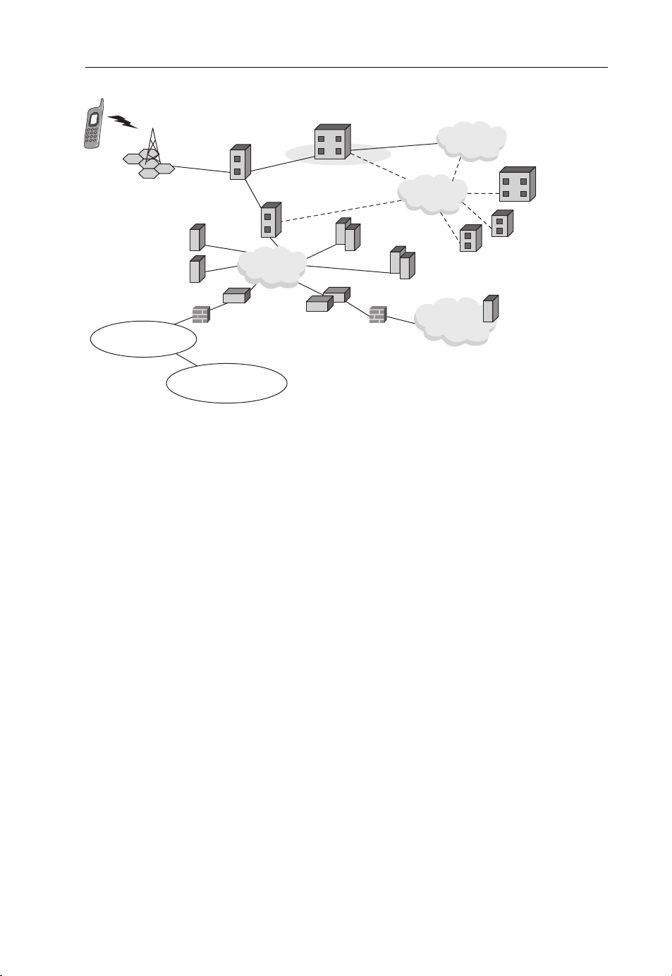
GSM and EGPRS 45
MS
MSC
DNS
FW
SS7
Network
CG
Corporate
Intranet
PSTN
SMS - GMSC
HLRAuC
EIR
PTM SC
Inter PLMN
Backbone
BTS
LIG
FW
Operator B
BSC
SGSN
PLMN
GPRS IP
Backbone
Network
BG
GGSN
Figure 2.14 GPRS network.
EDGE and EGPRS are interchangeably used to refer to the same technology. The reader
should make no distinction between the two terms used in this book.
2.4.1 EGPRS Network Elements
In simpler terms, addition of the packet core elements to a conventional GSM network would
convert it into an EGPRS network. The new elements, as seen in Figure 2.14, are the Mobile
Station (MS), Serving GPRS Support Node (SGSN), GPRS Gateway Support Node (GGSN),
Border Gateway (BG), Legal Interception Gateway (LIG), Domain Name System (DNS) and
Packet Control Unit (PCU).
2.4.1.1 Mobile Station (MS)
The main difference between the GSM and GPRS mobiles is the data capability. The GPRS
mobile is capable of handling data at higher speeds. There are three classes of GPRS mobiles:
class A, class B and class C. Class A mobiles can be used on either networks simultaneously,
Class B can be connected on both networks but used only on one at a time while Class C can
only be used on either one of the networks.
Serving GPRS Support Node (SGSN)
The SGSN connects the BSC and GGSN while serving as an access point of to the GPRS
mobile station for the GPRS network. This element is responsible for functions such as
authentication and mobility management.
Page 70

46 Cellular Technologies for Emerging Markets
GPRS Gateway Support Node (GGSN)
The GGSN connects the GPRS network to the external networks, for example Internet and
X.25, and acts as a sub-router from the perspective of external networks. It also acts as a ‘wall’
to the external networks to protect the GPRS network.
2.4.1.2 Border Gateway (BG)
This element is responsible for secure connections between various PLMNs over the interPLMN backbone network. The BG contains security features, firewalls, etc.
2.4.1.3 Legal Interception Gateway (LIG)
As the name suggests, this element is required for delivering the intercepted user information
to the legal agencies (law enforcement agencies).
2.4.1.4 Domain Name System (DNS)
This element is responsible for mapping the domain name to the IP address. In the GPRS
network, it is used to map logical access point names (APNs) to the GGSN IP addresses.
2.4.1.5 Packet Control Unit (PCU)
This unit is physically located in the BSC and is responsible for the packet control related
functions in the BSC.
2.4.2 Interfaces in the EGPRS Network
Apart from the interfaces discussed above in conventional GSM networks, there are a few
more interfaces in the packet core network (see Figure 2.15).
2.4.2.1 G
This is the interface between the BSC and SGSN. It carries the GPRS traffic and signalling
between the BSS and GPRS packet core network.
2.4.2.2 G
Within same PLMNs, the interface between two GSNs is the G
and signalling interface intra-PLMN backbone.
Interface
b
Interface
n
interface. It provides the data
n
Page 71

GSM and EGPRS 47
SMSGMSC
MSC/
VLR
SMS-1WMSC
G
s
HLR
G
d
G
r
SGSN
G
b
SGSN
G
n
G
GGSN
Other PLMN
G
n
GGSNBSS
G
f
p
EIR
G
i
PDN
Figure 2.15 GPRS interfaces.
2.4.2.3 Gb Interface
This is the interfacebetween theBSS andSGSN. It carries the trafficand signallinginformation
between the BSS (of the GSM) and the GPRS network.
2.4.2.4 Gn Interface
This is the interface between the SGSN and SGSN/GGSN of the same network. This provides
data and signalling for intra-system functioning,
2.4.2.5 Gd Interface
This is present between the SMS-GSMC/SMS-IWMSC and SGSN, thus providing a better
use of the SMS services.
2.4.2.6 Gp Interface
This is the interface between the SGSN and the GGSN of another PLMN – an interface
between the two GPRS networks.
2.4.2.7 Gs Interface
This is the interface between the SGSN and MSC/VLR. Location data handling and paging
requests through the MSC are handled via this interface.
Page 72

48 Cellular Technologies for Emerging Markets
2.4.2.8 Gr Interface
This is the interface between the SGSN and HLR through which all the subscriber information
can be assessed by the SGSN from the HLR.
2.4.2.9 Gf Interface
This interface gives the SGSN the equipment information that is present in the EIR.
2.4.2.10 Gi Interface
This is the interface between the GGSN and the external networks. This is not a standard
interface, as the specifications woulddepend uponthe type of interface thatwould beconnected
to the GPRS network.
2.4.3 Channels in the EGPRS Network
Moving onto the existing channels in the GSM network which are voice channels, there are
some new channels in a GPRS network that are related to the packet functionality. These
logical channels are allocated to the physical channel called the PDCH (packet data channel)
(see Table 2.5).
Channel allocation in the EGPRS (EDGE) network is similar to that of the GPRS network.
The PACCH is the only associated channel when physical resources are assigned while the
BCCH, PCH, RACH and AGCH are signalling channels.
Table 2.5 EGPRS channels
Channel Abbreviation Function/Application
Packet Broadcast Control Channel (DL) PBCCH Broadcast system information specific to
packet data
Packet Access Grant Channel (DL) PAGCH Notifies that mobile about resource
assignment before actual packet transfer
Packet Notification Channel (DL) PNCH Used for sending information to multiple
mobile stations
Packet Paging Channel (DL) PPCH Pages a mobile station before packet
transfer process begins
Packet Random Access Channel (UL) PRACH Used by the mobile station for
initialization of the uplink packet transfer.
Packet Common Control Channel PCCCH Contain logical channels for common
control signalling
Packet Data Traffic Channel PDTCH Channel temporarily used for data
transfer
Packet Associated Control Channel PACCH Used for signalling information transfer
for a given mobile
Page 73

GSM and EGPRS 49
Table 2.6 Coding schemes for the GPRS network
Data Rates (kbps)
Coding
Schemes Code Rate
CS-1 1/2 9.05 8
CS-2 ∼2/3 13.4 12
CS-3 ∼3/4 15.6 14.4
CS-4 1 21.4 20
Data Rates
(Kbps)
(excluding headers:
RLC/MAC)
2.4.4 Coding Schemes
There are four coding schemes in the GPRS network (see Table 2.6), that is CS-1, CS-2, CS-3
and CS-4. In CS-1, a half-rate convolution coding is used for forward-error correction and has
a data rate of 9.05 kbps. Both the CS-2 and CS-3 are similar to CS-1 except that ‘puncturing’
is used. This technique increases the data rates at the expense of redundancy. With no FEC
in CS-4, the data rate is further increased. Since the EGPRS system is an enhancement to the
GPRS system, the data rates increase to 59.6 kbps.
The first four coding schemes are still GSMK while the last five are 8-PSK (see Table 2.7).
In GPRS systems, the modulation used is GMSK while in the EGPRS system the modulation
used is 8-PSK. Apart from data rates system, a couple of other features (link adaptation and
incremental redundancy) make the EGPRS systems much more attractive.
Link adaptation is used for maximizing the channel throughput with the lowest amount
of delay in the changing climatic conditions. Thus, the link adaptation features try to maintain the quality of the signal in adverse conditions. Incremental redundancy (IR) improves
the throughput and this is done by automatically adapting the total amount of transmitted
redundancy to the radio channel conditions. This is carried out by using two techniques:
ARQ (Automatic Repeat reQuest) and FEC (Forward Error Correction). The ‘power control
feature’ in EGPRS systems is more complicated than in GSM systems due to addition of the
data. Uplink power control is used to reduce interference (and increase mobile battery life)
while the downlink power control reduces the power of the BTS and hence the interference
in the network. TBF (Temporary Block Flow) is another concept in EGPRS networks. This is
Table 2.7 Coding schemes for the EGPRS network
MCS Modulation User Rate
1 GMSK 8.8 kbps
2 GMSK 11.2 kbps
3 GMSK 14.8 kbps
4 GMSK 17.6 kbps
5 8-PSK 22.4 kbps
6 8-PSK 29.6 kbps
7 8-PSK 44.8 kbps
8 8-PSK 54.4 kbps
9 8-PSK 59.2 kbps
Page 74

50 Cellular Technologies for Emerging Markets
defined as the temporary connection that is established for the data flow between the network
and mobile station.
2.5 EGPRS Network Design and Optimization
The planning process in an EGPRS network is similar to that of GSM networks. However,
some important changes are highlighted here. As mentioned before, the main planning tasks
are coverage, capacity, frequency and parameter planning
The main task in coverage planning is to provide coverage planning for both uplink and
downlink in a balanced way (using link budget calculations). This means in practice keeping
the provision of sufficient Carrier-to-Noise(C/N) ratios across thecoverage area for successful
data transmission, on both the uplink and downlink. Each of the coding schemes, CS/MCS,
defined ina EGPRS system is suitedfor a particular coverage area, that isas the coding scheme
goes higher (more data being transmitted), the coverage area becomes smaller (as shown in
Figure 2.16). One important aspect of the link budget is that the for CS-2, body loss is not
used, hence giving a 3 dB advantage. The EGPRS system is an ‘interference-limited system’
rather than a ‘frequency-limited system’. In the GPRS system, CS-3 and CS-4 implementation
has many requirements; hence usually CS-1 and CS-2 are implemented.
For capacity planning, the fundamental change from the GSM system is that the EGPRS
system carries three types of traffic: voice, CS-data and PS-data. CS traffic always has a higher
priority than the PS traffic. Some of the PS traffic are ‘delay-sensitive’ and hence, dedicate
timeslots are used to carry it. The EGPRS system has higher data rates, that is an average
throughput per radio timeslot changes. However, the concept of dedicated and default (for
E.
12 000
000
11
000
10
9000
8000
7000
6000
2000 3000 4000 5000 6000 7000
CS-1
CS-2
CS-3
CS-4
2
m
8000 9000 10
Figure 2.16 Coverage areas of different GPRS coding schemes.
000 11 000
Page 75

GSM and EGPRS 51
voice and CS-data) territory remains the same for EGPRS system. The main parameters used
when planning for capacity in EGPRS networks are as follows:
r
peak circuit-switched traffic load (erlangs);
r
peak packet-switched load (kbps);
r
packet-switched load during overall traffic peak hour (kbps);
r
circuit-switched traffic load during overall traffic peak hour (erlangs).
CS traffic calculations are similar to that of GSM networks using erlang B tables, blocking and
C/I thresholds. For PS traffic, the dedicated territory is used and for CS and voice, the default
territory is used. It is possible to upgrade and downgrade EGPRS territories in cases where CS
traffic decreases and increases. The data throughput is one of the key indicators of a EGPRS
network (after all, a EGPRS network is installed for catering to the data users). The number
of users will define the throughput capacity of the network. As mentioned above, the more the
number of data users, the less would be the coverage and a lesser number of users would be
able to access higher capacity, that is higher data rates. Under ‘busy conditions’, several users
may use the same timeslot. Here, the concept of the rate reduction factor (RRF) comes into
play which can be quantified by using the effective reduction from the rate achievable at low
loads for the given GPRS territory occupancy. This leads to Quality of Service (QoS) that is
offered to EGPRS subscribers. During dimensioning for a given QoS, RRF can be used. This
gives an estimate of how well an EGPRS territory can be loaded before the QoS offered to
users is degraded to an unacceptable level.
Coverage and frequency planning go hand-in-hand as in the GSM network. The EGPRS
system is an interference-limited system and not a noise-limited system. Frequency planning
and power control are a couple of methods used to reduce interference in a EGPRS network.
Frequency planning in a EGPRS network is similar to that of a GSM network. Power control
is more important in the downlink direction and is accomplished by using the BCCH layer.
The transmission planning process in a EGPRS network is similar to that for a GSM
network. However, due to addition of packet data, there are a few additions in planning that
include dimensioning of dynamic Abis (this is a vendor-specific feature) and dimensioning
of the packet control unitin the BSC.There are few timeslotson the Abis that are dedicated for
the PS traffic. Due to this, the number of TSs for the Voice and CS data decreases and hence
the number of voice users decreases. Usually, in the EGPRS network, especially sites that
are hotspots, the capacity of E1 is increased from the usual 1E1 to 2E1s. The concept behind
dynamic Abis dimensioning is to find the number of timeslots that can be assigned to a pool in
such a manner that the Abis does not become a limitation for the air-interface throughput. The
main inputs forthis wouldbe the number ofradio timeslotsrequired for PS traffic(i.e. dedicated
and default territories in an EDGE radio network), capacity of radio timeslots, blocking that
could take place on the Abis-interface, etc. Based on these inputs and the number of PCM
timeslots available for the pool, the required number of PCM timeslots can be calculated.
Equipment limitations and capability should, however, be kept into consideration.
From thecore network planning perspective, PCU dimensioning,Gb-interface planning and
SGSN dimensioning are the key aspects. Based on the capacity of the BSC, inputs such as
the number of TRXs that can be supported, amount of the traffic handled and the number of
traffic channels that can be handled would lead to the number of PCUs that would be needed
to support the traffic. Gb-interface dimensioning would come up with the number of E1s that
Page 76

52 Cellular Technologies for Emerging Markets
would be needed between the PCU and SGSN. The total number of subscribers, processing
capacity of the SGSN and interface capacity would lead to the number of SGSNs needed in
the network. Dedicated PCM links (also known as ‘Frame Relay Links’) could be used to send
the packet data from the BSC to the SGSN. The main result of the frame relay dimensioning
is to find the number of timeslots that are needed to send the packet data traffic from the BSC
to the SGSN.
2.5.1 Parameter Tuning
The key parameters in the EGPRS systems are the same as in the GSM systems; however, with
the addition of a PS core network, packet data-related parameters are new additions to the list.
2.5.1.1 GPRS Enabled
This parameter defines whether the cell/radio is allowed to handle GPRS traffic.
2.5.1.2 Default GPRS Capacity
This represents timeslots that are always allocated to the GPRS territory unless preempted by
CSW traffic.
2.5.1.3 Dedicated GPRS Capacity
This represents the number of TCHs which can be ‘dedicatedly reserved’ for GPRS use and
is thereby removed for circuit-switched traffic.
2.5.1.4 Additional GPRS Capacity
This represents the additional timeslots, over and above the default territory, that may be used
by GPRS traffic, if circuit-switched traffic permits (see Figure 2.17).
2.5.1.5 Maximum GPRS Capacity
This represents the maximum number of timeslotsin a given cellthat can be used up for GPRS
traffic.
2.5.1.6 GPRS Traffic Preference
This decides if GPRS traffic should be assigned to the BCCH carrier prior to other TCH
carriers within the same cell.
Page 77

GSM and EGPRS 53
TRX 1
TS
TS
BCCH PBCCH TS TS TS TS TS TS
TSTRX 2
Dedicated (fixed)
Default (dynamic)
territory, etc.
TS TS TS TS TS TS TS
Figure 2.17 GPRS timeslot allocation to CS and PS traffic.
PST
CST
2.5.1.7 Territory Update Guard Time
This determines a timer value, that is the ‘guard time’ between two subsequent territory
updates.
2.5.1.8 Intracell Handover for GPRS Territory Upgrade
During the GPRS territory upgrade procedure, CS calls in the timeslots to be included in the
territory are handed over to other available timeslots in the same cell.
There are a few more parameters in the EGPRS transmission and core network. The major
ones are related to the concepts of EDGE territory, Dynamic Abis, BLER (Block Error Rate),
MCS schemes, BCCH usage, etc. These are the parameters that directly influence the actual
throughput and latency (and ultimately end-user application throughput). The parameters
related to TBF (Temporary Block Flow) include the TBF set-up success rate, TBF drops and
TBF blocking. Based on this parameter monitoring, tuning is carried out in order to bring the
network up to the highest quality standards.
Coverage in the GSM, as well as in the GPRS networks, is dependent on the C/I ratios. With
the EGPRS network by utilizing the resources of the GSM network, the interference would be
high, thus degrading the C/I ratio. Degradation of the C/I ratio would in turn mean a reduction
in the coverage areas. Moreover, the addition of the GPRS network would decrease the voice
quality of the network.
In urban areas, there is always a problem of frequencies. The channel allocation to the
EGPRS network in the initial phase is always based upon the GSM channel allocation, that is
voice (CS) subscribers taking a priority. Thus, capacity plans and the channel allocations have
to be studied and optimized again during this process.
Another aspect is the speed of the data services. Although the theoretical speed of a EGPRS
network should be about 171 kbps, the practical values are still around 40–60 kbps. A speed
of 171 kbps is possible only when all of the eight timeslots are utilized, which is not the case
as usually 5 TS can be used for data. Moreover, the C/I requirements may not be satisfied for
coding schemes beyond CS-1, thus reducing the data processing scheme.
Page 78

Page 79

3
UMTS
3.1 The 3G Evolution – UMTS
In Chapter 2, we saw the evolution of the systems from 1G to 2G or rather to 2.5G. Second
generation (2G) systems were developed with transparency and compatibility in mind; these
are semi-global systemand definitelyfar better anddevelopedthan thefirst generation analogue
systems. One of the most famous technologies was the GSM system which we have already
seen in the previous chapter. The next generation or third generation (3G) technology has
been developed to fulfil the dream for a truly global system – based on footprints of already
successful GSM systems in terms of the system being fully specified and the interface being
standard and open. However, due to drastic changes, third generation systems are much more
superior to the second generation systems. The bit rates go up to 2 Mbps (with HSPA up to
42 Mbps). The data services offered are both in real time and non-real time with variable data
rates (bandwidth on demand). The quality of service and spectrum efficiency is high and at the
same time, multiplexing of various services with varying quality requirements on one channel
is possible.
3GPP or the 3rd Generation Partnership Project is a collaboration agreement between
various telecommunication organizations, such as ARIB, CCSA, ETSI, ATIS, TTA and TTC,
established in 1998. The main job of 3GPP was to come up with the technical specifications
that would be globally applicable for 3G networks. The 3GPP specifications were to be based
on GSM specifications. 3GPP consists of Project Co-ordination Groups (PCGs) and Technical
Specification Groups (TSGs), as shown in Figure 3.1.
The specifications of 3G are called ‘releases’ and each of these releases incorporate many
documents/standards. Release 1 was called ‘Release98’, ‘Release2000’ wascalled ‘Release 4’
and after that it was ‘Release 5’, ‘Release 6’ and ‘Release 7’. 3GPP’s releases beyond ‘Release
7’ are called LTE (Long Term Evolution) systems – these are different systems with different
air-interfaces. The first release is specified in ‘Release 8’ but there are specifications for
WCDMA in ‘Release 8’ (covered later in this book). ‘Release 98’ concerned the pre-3G, that
is GSM network. It was only in ‘Release 99’ that the first UMTS networks were specified. The
main feature of ‘Release 99’ was the creation of UTRA (Universal Terrestrial Radio Access).
Other features included LCS, CAMEL, narrowband AMR, etc. ‘Release 4’ came up with features such as bearer-independent CS network architecture, streaming, multimedia messaging,
Cellular Technologies for Emerging Markets: 2G, 3G and Beyond Ajay R. Mishra
C
2010 John Wiley & Sons, Ltd
Page 80

56 Cellular Technologies for Emerging Markets
Project Coordination Group
TSG
Radio
Access
Network
Figure 3.1 3GPP structure [www.3gpp.org].
TSG
Core
Network
TSG
Terminals
TSG
Service and
System
Aspects
GERAN, etc. ‘Release 5’ introduced IMSs (IP-based Multimedia Services), Wideband AMR,
GTT (Global Text Telephony), HSDPA, etc. ‘Release 6’ introduced HSUPA, Push-to-Talk over
cellular (enhancements to IMS), etc. ‘Release 7’ concerned HSPA+, real-time applications
such as VoIP, etc.
3GPP has five main standardization areas: terminal, radio, core, services/systems and
GERAN. The terminal groups are responsible for standardization work related to terminals
such as USIM to the mobile interface, messaging, conformance testing, service capability protocols, etc. Theradio groupis responsible for the specifications related to air-interfaces (I
), BTSradio performance, conformance testing, layers 1, 2and 3 specifications, etc. The core
I
u
ub,Iur
group has thespecification responsibilityrelated topacketdata, inter-working function between
core and external network, signalling, etc. The services and systems groups look into specifications development related to services, evolutions, charging, accounting, architecture, etc.
UMTS (Universal Mobile Terrestrial System) is one of the 3G technologies. Because of
the nature of 3G technology and its evolution from GSM, UMTS is also called 3GSM. The
catalogue of 3G within the ITU is called the IMT-2000 or International Mobile Telecommunications for 2000 MHz. Several different proposals for the air-interface were incorporated.
WCDMA (used in Europe, Asia, Japan and Korea) uses the frequency bands allocated by
WARC-92. In North America, these bands were already used and hence 3G services are
implemented, replacing part of the spectrum, a technique called ‘re-farming’. TD-CDMA
contains the time division duplex components of UMTS and Chinese TD-SCDMA (integrated with UMTS-TDD). UWC-136 system has been included in the IMT-2000 group –
this is TDMA-based and an enhancement of IS-36 and GSM. For low-mobility applications,
DECT (Digital Enhanced Cordless Telecommunication) has been adopted. This is based on
FD TDMA. UMTS uses WCDMA as its air-interface technology. The frequency band of
175 MHz has been reserved for 3G systems (for GSM, 220 MHz is reserved in Europe).
The range for 3G systems extends from 1880–1980 MHz, 2010–2025 MHz and 2110–2170
MHz, along with two 30 MHz segments for satellite-based systems. The UMTS system uses a
channel bandwidth of 5 MHz. There are seven unpaired channels within 1900–1920 MHz and
2010–2025 MHz, implying that one 5 MHz has to implement in both the uplink and downlink directions. Between 1920 to 1980 MHz and 2110 to 2170 MHz, there are twelve paired
frequency bands available (5 MHz each). However, in Japan 1900–1920 MHz is occupied for
the Personal Hand Phone Service (PHS) and hence not available for 3G; similarly this is the
case in the USA. This means that Europeans and Japanese systems would not be operational
,
Page 81

UMTS 57
800
850 900 950 1000 1700 1750 1800 1850 1900 1950 2000 2050 2100 2150 2200 2500 2550 2600 2650 2700
ITU
Alloc.
Europe
China
Japan,
Korea
w/o PHS
North
America
IMT 2000 IMT 2000
GSM 1800 UMTS
GSM 1800. PCS
Cellular
Cellular
GSM
GSM
PDC
IMT 2000
D
E
G
1
IMT 2000
P
H
IMT 2000
S
P C S
AB C AB C
M
S
S
M
S
S
M
S
S
M
S
S
M
S
S
IMT
2000
UMTS
IMT
2000
IMT
2000
Re-
serve
M
S
S
M
S
S
M
S
S
M
S
S
MSS: Mobile
Satellite Systems
M
S
S
IMT 2000
UMTS
Figure 3.2 WRC-2000 IMT-2000 frequencies [www.itu/newsarchive/wrc2000/presskit/IMT-2000.
html].
in the USA. The Federal Communications Commission has allocated 1915–1920 MHz with
1995–2000 MHz and 2020–2025 MHz with 2175–2180 MHz for advanced wireless system
use. However, government and regulatory bodies are working on spectrum issues. Frequency
allocation according to WRC 2000 is shown in Figure 3.2.
UMTS frequencies can be summarized as follows:
r
1920–1980 and 2110–2170 MHz: (FDD, W-CDMA), paired uplink and downlink, channel
spacing is 5 MHz. Operator requires 3–4 channels (2 ×15 MHz or 2 × 20 MHz) to build a
high-speed, high-capacity network.
r
1900–1920 and 2010–2025 MHz: (TDD, TD/CDMA), unpaired, channel spacing is 5 MHz.
Transmission and receiving are not separated in frequency.
r
1980–2010 and 2170–2200 MHz: for satellite uplink and downlink.
3.2 UMTS Services and Applications
A modern telecommunication network such as UMTS can provide a wide variety of services.
The service concepts and definitions of UMTS are mostly taken from GSM. The service
parameters are often fixed in GSM, while they can be dynamically renegotiated in UMTS. The
services provided by UMTS can be divided into four main classes (3GPP TS 23.107).
3.2.1 Teleservices
A teleservice is a type of telecommunication service that provides the complete end-to-end
capability for communication between mobileusers inaccordance with standardized protocols.
Page 82

58 Cellular Technologies for Emerging Markets
The user has no direct responsibility for the end-point applications. Teleservices make use
of the whole OSI model protocol stack and also include the terminal equipment functions.
Teleservices utilize the bearerservices provided by thelower layers (except forcircuit-switched
speech services).
3.2.2 Bearer Services
Bearer services are basic telecommunication services that offer the capability of the pure
transmission of signals between access points. These services can be either circuit-switched
or packet-switched. Bearer services concern the three lowest layers of the OSI model. They
are end-to-end transport services in which the user is responsible for the end-point entities.
A bearer service is defined using a set of characteristics that make it different from all the
other bearer services. These service characteristics define such things as the traffic type, the
traffic characteristics and the supported bit rates. UMTS allows for the negotiation of these
parameters between the application and the network. There is a negotiation routine in which
the application requests a certain bearer service, and the network checks the availableresources
and thengrants the requested service orsuggests a lower levelof service. The application atthe
user side either accepts or rejects the network’s suggestion. It also renegotiates the properties
of abearer service during an active connection in UMTS.This makes the UMTS bearerservice
much more flexible and allows the network resources to be much better utilized.
3.2.3 Supplementary Services
A supplementary service (SS) complements and enhances bearer services and teleservices.
They cannot exist without these basic services, that is there are no stand-alone supplementary
services. Supplementary services reside in the switch and may supplement several basic
telecommunication services. Also, one basic telecommunication service may simultaneously
use several SSs. The latter case requires that the interactions between active SSs be carefully
specified.
3.2.4 Service Capabilities
Service capabilities are a set of building blocks that can be used to implement value-added
services. As the value-added services are not standardized, it is possible to implement them in
a way that produces unique services. The latter are more likely to attract and hold subscribers
than constant ‘price wars’ among operators with identical services. Service capabilities are
accessible to applications via a standardized application interface.
According to the UMTS Forum, the 3G data services are divided into three categories:
content, connectivity and mobility. These are sub-divided into six categories: mobile Internet
access, location-based services, multimedia messaging, mobile Intranet, customized ‘infotainment’ and ‘rich voice’. UMTS offers teleservices, for example speech and SMS and bearer
services. Thecharacteristics of the bearer servicescan be negotiated before the sessionsor during on-going sessions for both point-to-point and point-to-multipoint communications. These
bearer services have different parameters for Quality of Service (QoS) such as BER (Bit Error
Rate), Maximum Transfer Delay, etc. QoS is defined end-to-end, that is one user equipment to
Page 83

UMTS 59
UMTS
TE MT UTRAN
End-to-End Service
TE/MT Local
Bearer Service
Radio Access Bearer Service
Radio Bearer
Service
UTRA
FDD/TDD
Service
UMTB Bearer Service
lu Bearer
Service
Physical
Bearer Service
CN Iu
EDGE
NODE
CN Bearer
Backbone
Bearer Service
Service
CN
Gateway
TE
External Bearer
Service
Figure 3.3 QoS architecture. © 2009. 3GPPTMTSs and TRs are the property of ARIB, ATIS, CCSA,
ETSI, TTA AND TTC who jointly own the copyright in them. They are subject to further modifications
and are therefore provided to you “as is” for information purposes only. Further useis strictly prohibited.
another user equipment. As shown in Figure 3.3, each bearer service offers individual services
by using the services offered by layers below and at the same time including all aspects (control
signalling, user plane transport, QoS management, etc.) to enable the provisions of contracted
QoS.
3.3 UMTS Bearer Service QoS Parameters
Traffic type. Thisparameter isintended todescribe the characteristics of the source, forexample
background, interactive, streaming, conversational.
Maximum bit rate. This is the maximum number of bits delivered by UMTS and to UMTS
at an SAP within a period of time, divided by the duration of the period. The maximum bit
rate is the upper limit a user or application can accept or provide. Practically, the maximum
bit rate can be used to make code reservations in the downlink of the radio interface.
Guaranteed bit rate. This is the guaranteed number of bits delivered by the UMTS at an
SAP within a period of time divided by the duration of the period. This describes the bit rate
that the UMTS bearer service should guarantee to the user or applications.
Delivery order (Y/N?).This indicates whether theUMTS bearershould provide, in sequence,
SDU delivery or not. This is derived from the user protocol (PDP type) and specifies if
out-of-sequence SDUs are acceptable of not.
Page 84

60 Cellular Technologies for Emerging Markets
Maximum SDU size. The maximum SDU size allowed (for admission control and policing).
SDU format information. This is the list of possible exact sizes of the SDUs, in bits. This
information is needed by UTRAN to be able to operate in the transparent RLC protocol mode
which is beneficial to spectral efficiency and delay when RLC re-transmission is not used.
SDU error ratio. The fraction of SDUs lost or detected as erroneous and which is needed
for conforming traffic.
Residual bit error ratio. This indicates the undetected bit error ratio in the delivered SDUs.
If no detection is requested, the residual bit error ratio indicates the bit error ratio in delivered
SDUs. This is used to configure radio interface protocols, algorithms and error detecting
coding.
Delivery of erroneous SDUs (Y/N?). This indicates whether the SDUs detected as erroneous
should be delivered or discarded. This is used to decide whether or not error detection is
needed and whether the frames with detected errors should be forwarded or not.
Transfer delay (ms). This indicates the maximum delay for the 95th percentile of the
distribution of delay for all delivered SDUs during the lifetime of a bearer service, where
delay for an SDU is defined as the time from a request to transfer an SDU at one SAP to
its delivery at the other SAP. This is used to specify the delay tolerated by the application. It
allows UTRAN to set transport formats and ARQ parameters.
Traffic handling priority. This specifies the relative importance for handling of all the SDUs
belonging to the UMTS bearer compared to the SDUs of other bearers. Within the interactive
class, there is a definite need to differentiate between bearer qualities. This is handled by
using the traffic handling priority attribute, to allow UMTS to schedule traffic accordingly. By
definition, priority is an alternative to absolute guarantees, and thus these two attribute types
cannot be used together for a single bearer.
Allocation/retention priority. This specifies the relative importance compared to other
UMTS bearers for allocation and retention of the UMTS bearer. The allocation/retention
priority attribute is a subscription attribute which is not negotiated from the mobile terminal. This priority is used for differentiating between bearers when performing allocation and
retention of a bearer
3.4 QoS Classes
These are also called traffic classes (see Table 3.1). The main differentiation between the
various traffic classes is the ‘delay sensitivity’. There are four QoS classes defined in the
UMTS standards (3GPP TS 23.107):
r
conversational;
r
streaming;
r
interactive;
r
background.
3.4.1 Conversational Class
As the name suggests, this is for applications related to ‘real time conversations’, for example
speech, VoIP, video conferencing, etc. The constraints in terms of delay are given by human
Page 85

UMTS 61
Table 3.1 UTMS QoS classes. © 2009. 3GPPTMTSs and TRs are the property of ARIB, ATIS,
CCSA, ETSI, TTA AND TTC who jointly own the copyright in them. They are subject to further
modifications and are therefore provided to you “as is” for information purposes only. Further use is
strictly prohibited
Traffic class
Fundamental
characteristics
Example of the
application
Interactive class
Conversational class
conversational RT
Preserve time
relation (variation)
between information
entities of the stream
Conversational
pattern (stringent
and low delay)
Voice Streaming video Web browsing Background
Streaming class
streaming RT
Preserve time
relation (variation)
between
information entities
of the stream
Interactive best
effort
Request response
pattern
Preserve payload
content
Background
Background best
effort
Destination is not
expecting the data
within a certain
time
Preserve payload
content
download of emails
interactivity. This class is characterized by a very low tolerance level in terms of delay and
any failure to provide a low enough transfer delay would lead to a degraded quality of
service. The fundamental QoS characteristics are as follows: preserve time relation (variation) between information entities of streams and conversational pattern (stringent and low
delay).
3.4.2 Streaming Class
Downloading of the real time video/audio stream falls under the streaming class. It is one way
data flow (unidirectional) and is aimed at ‘love’ (human) destinations. It is characterized by
the time variations between information entities (i.e. samples, packets) within which a flow is
preserved, though it does not have any requirements on low transfer delay.
3.4.3 Interactive Class
Examples like web browsing, remote terminal emulation, database retrieval, etc. best describe
this class. Inthis class,the human interactionis toa machine located ata distance. Telemachines
are also typical example of this class of service. The round trip delay time is a key attribute of
this class. The fundamental QoSs of this class are the request response pattern and the preserve
payload content.
3.4.4 Background Class
In thisclass, the destination is not expecting the data withina certain time frame, that is delayis
not a concern. Computer-delivering e-mails, SMSs, downloading of databases, etc. are typical
examples of this class. The fundamental QoSs for this service are preserving payload content
and not expecting data within a certain time frame.
Page 86

62 Cellular Technologies for Emerging Markets
3.5 WCDMA Concepts
3.5.1 Spreading and De-Spreading
As discussed before, WCDMA has higher bit rates of 2 MHz. This means that a larger
bandwidth is required to support such higher bit rates and in this case, it is 5MHz. The
user information bits are spread over a large bandwidth by multiplying this user information with ‘quasi-random’ bits called ‘chips’. As the actual information is transmitted on a
wider bandwidth the system become tolerant towards the narrowband interfering signals, in
the process solving the problems of the number of subscribers that could simultaneously
be logged to the network in the TDMA and FDMA systems. The spread spectrum technique
thus allows efficient use of the spectrum and allows multiple numbers of users to use the
system simultaneously – in the same frequency band. One of the most common techniques
used is the ‘direct sequence’ CDMA or DS-CDMA. In this technique, the bipolar user data bit
stream is multiplied by the user-specific bipolar code sequence. This signal (i.e. multiplying
signal) is called the ‘code’. The rate at which the data spreads is called the chip rate. A BPSK
(Binary Phase Shift Keying) modulated signal is usually used as the original signal and the
second modulation is performed by multiplying the original signal with a sequence of bits
(of a wideband signal). This would spread the original signal, making it a wider bandwidth
signal. Each bit of the original signal is called the ‘symbol’ while that of the multiplying
signal is referred to as ‘chips’. The ratio of chip rate to symbol rate is called the ‘spreading
factor’ (SF). It is also defined as the factor by which the spectrum spreads. The multiplied
signal (this is different for every user) is transmitted over a bandwidth that is larger than what
would have been required to transmit the original data. Every user in the system uses this
process and at the same time leaves a user-specific code that would allow the transmitted
signal to be re-constructed (de-spreading) at the receiving end, as shown in Figure 3.4. All the
users in the network transmit at the same frequency, thereby increasing interference. When
the receiver receives the sum of several user signals, it is multiplied by the spreading code
while the respective user and the effect of other signals are removed. The output generated
from the received signal and the spreading code is integrated periodically for the duration of
the bit and the original signal is sampled at the end of the period.
SpreadingDe-spreading
Figure 3.4 Spreading/de-spreading phenomena.
Original
Signal
Code Signal
Spread Signal
Code Signal
Original
Signal
Page 87

UMTS 63
UMTS BS
F1
Code C
Code A
Code B
F1
Figure 3.5 Code assignment to subscribers.
Code D
Code E
UMTS BS
3.5.2 Code Channels
Unlike the GSM/ EDGE systems where the users are separated by frequency/time, in UMTS
systems, the users are separated by codes. Each user will have a unique code wherein the
signal from other users is seen as interference. This makes it an interference-limited system.
The spreading codes (codes A, B, etc., shown in Figure 3.5) are orthogonal to each other.
Although there is no co-relation between the codes, in some cases it can be so low that
the interference does not takes place between the users (these are called ‘quasi-orthogonal’
codes). The set of codes that are orthogonal/‘quasi-orthogonal’ to one another is called the
‘code family’. For mobile applications, large code families are used. The chip sequence is
dependent on the spreading factor (defined earlier) as the chip rate is higher by the spreading
factor than the bit rate. The orthogonal codes used are of variable spreading factors and are
called as OVSF codes or Orthogonal Variable Spreading Factor Codes. These codes can be
created using a code tree (as shown in Figure 3.6). Each node of the code tree has two branches
with a double length code and the same spreading factor. A code with an SF of N is created
from the code with an SF of N/2. Thus, at the kth level, a set of 2
k
length of 2
chips is available. There is one limitation though – two codes of different levels
of the code tree are orthogonal to one another only if one of the two codes is not the ‘mother
code’ of the other one. Due to this, the number of simultaneous codes depends on the bit rate
and spreading factor.
Apart from spreading, there are two other codes that should be known: scrambling and
channelization codes (spreading is done with the channelisation codes and scrambling with
the scrambling codes). The scrambling codes are used to separate the terminals and base
stations. During transmission, the spread signals are aggregated and then scrambled. The
process is done through chip-by-chip multiplications of the signal by a scrambling code that
has same rate as the spread chip streams – thereby not changing the signal bandwidth but
making them separable from each other. Due to this, the entire family of codes is available to
each transmitter. This helps in a way that two transmitters can use the same spreading codes
as the differentiation can be done by scrambling codes. Channelization codes are used for
separation from a single source. These are based on the OVSF technique, allowing the SF
k
spreading codes with a
Page 88

64 Cellular Technologies for Emerging Markets
SF = 4SF = 8SF = 16 SF = 256SF
C
(0) = (1111)
2
C
(1) = (11·1·1)
2
C
(2) = (1·11·1)
2
C2(3) = (1·1·11)
C
(0) = (11111111)
2
(1) = (1111·1·1·1·1)
C
2
C
(2) = (11·1·111·1·1)
2
C
(3) = (11·1·1·1·111)
2
(0) = (1·11·11·11·1)
C
2
C2(5) = (1·11·1·11·11)
C
(6) = (1·1·111·1·11)
2
(7) = (1·1·11·111·1)
C
2
(0) = (..........)
C
10
(1) = (..........)
C
10
C
(2) = (..........)
10
C
(3) = (..........)
10
(4) = (..........)
C
10
(5) = (..........)
C
10
(6) = (..........)
C
10
C
(7) = (..........)
10
(8) = (..........)
C
10
C10(9) = (..........)
C10(10) = (..........)
C
(11) = (..........)
10
C
(12) = (..........)
10
C
(13) = (..........)
10
C
(14) = (..........)
10
(15) = (..........)
C
10
C
o
(0) = (1)
= 2SF = 1
C
(0) = (11)
2
C
(1) = (1·1)
2
Figure 3.6 OVSF code tree.
to be changed while maintaining the orthogonality between different length spreading codes.
Both thespreading and uplink scrambling codes areallocated by the system, while indownlink
allocating the scrambling codes of the cells is a part of the network planning process.
3.5.3 Processing Gain
The amount by which the power density of the carrier signal is increased in the receiver is
called the processing gain and is dependent on the spreading factor. Due to the processing
gain, the system becomes more robust against interference. During the de-spreading phase, the
sum of the user and interfering signals is multiplied by the spreading code of the user which
helps in re-constructing the original signal. The bandwidth of the original signal is narrower
than the spread signal by an amount of the SF. However, the interfering signal spreads in the
receiver, thereby decreasing its power density by an amount of SF. This makes these systems
more robust against the narrowband interfering signals.
3.5.4 Cell Breathing
The load factor directly corresponds to the traffic supported by the cell. Due to changes in
the traffic load, the cell coverage area/ range changes. This is called ‘cell breathing’. For the
receiver to be guaranteed a sufficient quality of service, the service-specific C/I is maintained.
This is possible if the transmitter power is sufficient so that even in the case of attenuation,
Page 89

UMTS 65
25
20
15
UMTS BS
10
Loss (dB)
5
0
0
0.2
0.4
Load factor
0.6
0.8
1
Figure 3.7 Cell breathing.
the C/I can be guaranteed. But as the traffic grows in the network, interference increases.
This higher interference power would mean a decrease in received signal power and hence
the coverage area. However, this traffic load does not increase or decreases suddenly; it is
usually a gradual increase/decrease, as shown in Figure 3.7. Thus, the coverage also increases
or decreases gradually giving a ‘feeling’ that the cell is breathing. The intracell interference
is responsible for cell breathing. This interference is dependent on the receiver quality and
orthrogonality of the spreading codes.
3.5.5 Handover
There are a few types of handovers. Hard handover is defined as the handover between two
frequencies and is used in GSM. In UMTS,when a UEcommunicates to sectorsfrom different
base stations, it is called asoft handover (shown in Figure 3.8). A point to remember here is that
frequency does not change in the soft handover. In the hard handover, connection is switched
‘hard’, that is at a particular time while in the soft handover, there is no fixed switchover point
and the transfer from one base station to another is ‘soft’. Another kind of handover is the
Softer HO
(case 2)
Site1
Site2
Figure 3.8 Handover in the WCDMA radio network.
Soft HO
(case 1)
Page 90

66 Cellular Technologies for Emerging Markets
Fast Closed
Loop Power Control
DL Outer Loop
Power Control
Iub
BS
UE
Figure 3.9 Power control.
RNC
UL Outer
Loop PC
‘softer’ handover. In here, the transmission also takes place between the UE and the different
sectors ofsame base station. The mobiletakes twodifferent paths (interfaces) for communicating with thebase station;hence two different codesare used so thatthe mobilecan recognize the
different paths. There is not much difference in the downlink direction; however there is much
difference in the uplink direction for the two handovers. In the case of the soft handover, the
received signal is routedto the RNC fromboth the base stations sothat the best RNCcan take a
decision onkeeping thesignal which is giving a better quality. Asthis decision-making process
takes time (about 10–80 ms), double air-interface capacity is utilized by a single mobile for
one call. Hence, radio engineers have to take into account this process when doing the capacity
planning forthe radio network. About 30% of the links witnessthe soft handover phenomenon
against 10 % for a softer handover. The measurements generally include received signal code
power (signal power received on one code), signal power received within the channel bandwidth and Ec/No (ratio of received signal power to the received signal power indicator).
3.5.6 Power Control
The power control mechanism in the UMTS (shown in Figure 3.9) is quite important as it
prevents ‘near–far’ effects. In WCDMA networks, as the frequency re-use factor is unity, it
increases the importance of the fast and accurate power control mechanism. The closed loop
power control feature is used in these networks in the absence of which the mobile closer to
the base station will easily ‘over-shout’ the other mobiles in the cell, causing a blocking effect.
This is done by measuring the interference levels. Another type of power control feature used
is the ‘slow power control’ or ‘outer loop power control’ which maintains set quality.
3.5.7 Channels in WCDMA
There are three different types of channels: logical, transport and physical. Logical channels
are used with layer 2 for data transfer for higher layers. Transport channels are used for data
transfer between layer 2 and layer 1, while physical channels are used for data transfer for
Page 91

UMTS 67
Broadcast Control Channel (BCCH)
Control Channels
Dedicated Control Channel (DCCH)
Paging Control Channel (PCCH)
Common Control Channel (CCCH)
Traffic Channels
Figure 3.10 Logical channels (control and traffic).
Common Traffic Channel (CTCH)
Dedicated Traffic Channel (DTCH)
layer 2 and higher layers. Some of the key channels in each of the categories are described in
the following.
Logical channels consist of control and traffic channels. The logical channels are shown in
Figure 3.10.
Transport channels, like the logical channels, are of two types: dedicated transport channels
and common transport channels, based on the applications of the channels. The transport
channels are described in Figure 3.11.
There are two kinds of physical channels: dedicated and common channels. The transport
channels are mapped onto the physical channels (shown in Figure 3.12).
3.5.8 Rate Matching
The connection between the user terminal and the network is called the ‘bearer’. The bearer is
not fixedas inthe 2Gnetworks. In the 3G networks, thebearer isnegotiated and network checks
are available, plus resources and user subscriptions before allowing the bearer establishments.
The end-to-end services that the user uses define the base band data rate (in kbps), which will
use the negotiated bearer services. The base band data should then be protected from the errors
as they transmit from the terminal to the network radio terminal. It further adds significant
overhead to the original data, for example convolution coding may double or triple the original
base band bit rate. After error protection, the BB data rate is matched to the bearer data rate in
Common transport channels
Dedicated transport channels
Figure 3.11 Transport channels.
Broadcast Channel (BCH)
Paging Channel (PCH)
Forward Access Channel (FACH)
Random Access Channel (RACH)
Downlink Shared Channel (DSCH)
Dedicated Channel (DCH)
Page 92

68 Cellular Technologies for Emerging Markets
Synchronization Channel (SCH)
Common
physical channels
Common Pilot Channel (CPICH)
Acquisition Indicator Channel (AICH)
Paging Indicator Channel (PICH)
Primary Common Control Physical Channel (PCCPC)
Secondary Common Control Physical Channel (SCCPCH)
Physical Random Access Channel (PRACH)
Physical Downlink Shared Channel (PDSCH)
Dedicated
physical channels
Dedicated Physical Control Channel (DPCCH)
Dedicated Physical Data Channel (DPDCH)
Figure 3.12 Physical channels.
the WCDMA air-interface. This is called ‘rate matching’. The latter is carried out in order to
match the bits into the frames.
Difference between the Uplink and Downlink direction: the channel bit rate is different in
both of the directions, that is the uplink and downlink directions, although the system uses the
same spreading factor because of the difference in the modulation methods, channel coding,
interleaving and rate matching.
3.6 ATM
In ATM, the transfer mode is the one in which the information is organized into cells: it
is asynchronous in the sense that the recurrence of cells containing information from an
individual user is not necessarily periodic. Some of the basic characteristics that are offered by
the networks are to handle various types of traffic (voice, data – real-time and non-real-time)
and give reliability to usersat lowercosts. The ATM (Asynchronous Transfer Mode) technique
has these characteristicsand ishence chosen as the transmission technique of UMTSnetworks.
Frame relay and ATM are almost similar techniques, but as the frames in frame relay are of
variable length and hence variable delay, they are not suited for UMTS applications, while
the ATM is based on the ‘cell’ – small and fixed packets size making it ideal for UMTS
applications.
3.6.1 ATM Cell
An ATM cell consists of a 53 byte octet (octet header and 48 octet payload) as shown in
Figure 3.13. ATM technology is independent of the physical medium and is scalable, that is
multiplexing of the circuits leading to faster circuits is possible. Thus, ATM is a switching and
multiplexing technique capable of giving a desired quality of servicefor different applications.
The ATM cells (each cell being 53 bytes, with a 5 byte header and 48 byte payload) are
multiplexed to form virtual channels that are subsequently multiplexed to form various paths.
These paths are not permanent and are hence called ‘virtual’. These virtual paths are carried
Page 93

UMTS 69
5 byte header 48 byte payload
53 byte cell
Figure 3.13 ATM cell structure.
by the transmission media and their number may vary depending upon the capacity of the
transmission media.
3.6.2 Virtual Channels and Virtual Paths
As mentioned before, many virtual channels form one virtual path (shown in Figure 3.14).
Let’s now have a look into aspects related to virtual channels and virtual paths.
3.6.2.1 Virtual Channel
This is a sequence of the ATM cells belonging to a particular type of service or destination
which comprises the virtual channels.
3.6.2.2 Virtual Path
This is the number of VCs sharing one single link that ‘bundles’ different VCs into one path,
called the ‘virtual path’. Also, to simplify the routing and switching of cells belonging to a
particular destination and a particular type of service, VCs are combined into a single VP.
3.6.2.3 Virtual Channel Identifier
To identify a particular type of VC, the header of an ATM cell has a virtual channel identifier.
Virtual Path
Transmission
Path
Figure 3.14 Virtual circuits and virtual paths.
Virtual
Circuits
Page 94

70 Cellular Technologies for Emerging Markets
Higher layer-Control – Management
ATM adaptation layer
ATM layer
Physical Layer
Terminal Node Node Terminal
Figure 3.15 ATM protocol structure.
3.6.2.4 Virtual Path Identifier
To identify a particular type of VP, the header of the ATM cell has a virtual path identifier
(VPI).
3.6.3 Protocol Reference Model
The protocol reference model is shown in Figure 3.15.
3.6.3.1 Physical Layer
There are two sub-layers in the physical layer: TC (Transmission Convergence Layer) and PM
(Physical Medium Layer).
The TC layer is in charge of maintaining the cell rate by insertion and extraction of idle cells
in orderto adapt the rate ofATM cellsto the payload capacityof the transmission system. HEC
generation and verification perform error-free transportation of the headers. Cell delineation
is the mechanism that enables the receiver to recover the cell boundaries. It is based on the
identification of the header fields of the consecutive cells. If the HEC value is correct for
a certain number of consecutive cells, then the cell delineation mechanism is achieved. To
protect the cell delineation mechanism from malicious attack, the information is scrambled
before the transmission.
The PM layer includes only the physical medium-dependent function. Its specification then
depends upon the medium used. It provides the bit transmission capability, including bit
alignment. The physical medium can be fibre, co-axial cable, etc.
3.6.3.2 ATM Layer
The ATM layer is independent of the physical medium layer. The generic flow control is
defined at the B-ISDN UNI. The cell header generation and extraction function, except for
the HEC value, is applied at the termination point of the ATM layer. It includes both PT
and CLP bits. Cell VPI/VCI translations are performed at the ATM switching modes and/or
cross-connect nodes are to be encountered on a route from the transmitter to the receiver. The
cell mux/demux is based on the VCI/VPI values.
Page 95

UMTS 71
3.6.3.3 ATM Adaptation Layer (AAL)
With so many services requiring greater speeds, it would be suitable if the ATM provides them
a common platform to be transferred. But in spite of using different versions of ATM layers
for different services, another layer is introduced above the ATM layer that provides mapping
of different types of applications to the ATM layer. This layer is service-dependent. Thus,
the use of the ATM makes it mandatory for the need for an adaptation layer to support other
information-based protocols not based on the ATM.
AAL is sub-divided into the two logical sub-layers: SAR and CS. The SAR (segmentation
and re-assembly) sub-layer performs the segmentation and re-assembly of information in the
ATM cells. Segmentation means to segment higher layer PDUs into a suitable size for the
information fieldof the ATM cell (48octet) and receiving size the re-assemblyof the particular
information fields into higher layer PDUs. The CS (Convergence Layer) performs other service
adaptation. This layer is service-dependent. AAL functions are service-dependent. Connections falling into a particular class have similar QoS requirements. These classes can also have
their own buffers. Real-time classes will have shorter buffers than the delay tolerant classes.
The various services provided by the AAL (ATM Adaptation Layer) are as follows:
r
handling of transmission errors;
r
segmentation and re-assembly;
r
handling of lost cell conditions;
r
flow control and timing control.
Different types and quality of services would require different AAL protocols to support
the service. To minimize this wide variety of protocols, the ITU-T has defined four classes of
service thatcover a broadrange of applications. This classification isbased on three categories,
which have a timing relation between the source and the destination, the bit rate and finally
the connection mode. Based on these properties, different AAL protocols have been devised
which come under the four classes defined. Table 3.2 gives details of this service classification
as given by the ITU-T.
AAL Type 1
AAL type1, a connection-oriented service, is suitable for handling circuit emulation services,
such as voice and video conferencing. AAL1 requires timing synchronization between the
Table 3.2 AAL protocol classification as given by ITU-T. Reproduced from the International
Telecommunication Union (ITU)
Class A Class B Class C Class D
Timing relation between
source and destination
Bit rate Constant Variable
Connection mode Connection Oriented connection-less
AAL Protocol Type 1 Type 2 Type 3/4, Type 5 Type 3/4
Required Not Required
Page 96

72 Cellular Technologies for Emerging Markets
source and destination. For this reason, AAL1 depends on a medium, such as SONET, that
supports clocking.
AAL Type 2
The type 2 dealswith thevariable bit rate informationand isintended foranalogue applications,
such as video and audio that require timing information but do not require a constant bit rate.
AAL Type 3/4
AAL3/4 supports both connection-oriented and connection-less data. It was designed for
network service providers and is closely aligned with the Switched Multi Megabit Data
Service (SMDS). AAL3/4 is used to transmit SMDS packets over an ATM network.
AAL Type 5
AAL5 is the primary AAL for data and supports both connection-oriented and connection-less
data. It is used to transfer most non-SMDS data, such as classical IP over ATM and LAN
Emulation (LANE). AAL5 is also known as the simple and efficient adaptation layer (SEAL)
because the SAR sub-layer simply accepts the CS-PDU and segments it into 48-octet SAR
PDUs without adding any additional fields.
3.6.4 Performance of the ATM (QoS Parameters)
The parameters are defined by the ATM Forum and are shown in Table 3.3.
Constant bit rate (CBR). The user traffic is continuous and steady under CBR. Supported
by AAL1, this class has tight delay and delay variations bounds. Voice and video conferencing
are typical examples of CBR traffic.
Real-time variable bit rate (rt-VBR). Supported by AAL3/4 and AAL5, the nature of traffic
is ‘bursty’ and insensitive to smaller delay variations.
Non-real-time variable bit rate (nrt-VBR). This is similar to rt-VBR, except that the traffic
is ‘non-real time’. This class is used for frame relay inter-working. Both rt-VBR and nrt-VBR
have a variable bandwidth.
Unspecified bitrate (UBR).This is the best effort transmission. The user maymake arequest
for a maximum traffic rate, but the network provides the best rate possible. As in the above
two cases, AAL3/4 and AAL5 support this type of traffic.
Available bit rate (ABR). Under this, there is no guarantee of bandwidth. Also there is no
timing relationship between the source and destination.
Table 3.3 ATM QoS parameters
Service category Traffic parameters Qos parameters
CBR PCR CDVT max CTD ptp CDV CLR
rt-VBR PCR CDVT SCR MBS max CTD ptp CDV CLR
nrt-VBR PCR CDVT SCR MBS CLR — —
UBR PCR(opt) — — — — — —
ABR PCR MCR — — — — —
Page 97

UMTS 73
Sustainable cell rate (SCR). This is the upper bound on the average rate of the conforming
cells of an ATM connection, over time scales which are long relative to those for which the
PCR is defined.
Maximum burst size (MBS). This is the maximum number of cells that can be transmitted
on peak cell rate.
Minimum cell rate (MCR). This is the rate negotiated between the end-systems and the
network(s), such that the actual cell rate sent by the end-system on the ABR connection need
never be less than MCR.
The performance of the ATM layers can be measured by monitoring certain parameters.
These parameters can be divided into two groups: negotiable and non-negotiable.
Parameters that are negotiated are:
r
peak-to-peak cell delay variation (CDV);
r
maximum cell transfer delay (maximum CTD);
r
mean cell transfer delay (mean CTD);
r
cell loss ratio (CLR).
Cell delay variation. The CDV parameter describes variability in the pattern of cell arrival
(entry or exit) events at an MP (Measurement Point) with reference to the negotiated peak
cell rate 1/T (see Recommendation I.371); it includes the variability present at the cell source
(customer equipment) and the cumulative effects of variability introduced (or removed) in
all connection portions between the cell source and the specified MP. It can be related to
cell conformance at the MP, and to network queues. It can also be related to the buffering
procedures that might be used in AAL 1 to compensate for cell delay variation.
Cell transfer delay. Cell transfer delay (CTD) is the time, t2–t1, between the occurrence
of two corresponding cell transfer events, CRE1 at time t1 and CRE2 at time t2, where t2 >
t1 and t2–t1 ≤ Tmax. The value of T max is for further study, but should be larger than the
largest practically conceivable cell transfer delay.
Mean cell transfer delay. Mean cell transfer delay is the arithmetic average of a specified
number of cell transfer delays.
Cell loss ratio. Cell loss ratio (CLR) is the ratio of total lost cells to total transmitted cells
in a population of interest. Lost cells and transmitted cells in severely ‘errored’ cell blocks are
excluded from the calculation of cell loss ratio.
QoS parameters that are not negotiated are as follows:
r
cell error ratio (CER);
r
severely errored cell block ratio (SECBR);
r
cell mis-insertion rate (CMR).
Cell error ratio. The cell error ratio (CER) is the ratio of total errored cells to the total of
successfully transferred cells, plus tagged cells, plus errored cells in a population of interest.
Severely errored cell block ratio. The severely errored cell block ratio (SECBR) is the ratio
of total severely errored cell blocks to total cell blocks in a population of interest.
Cell ‘mis-insertion’ rate. The cell mis-insertion rate (CMR) is the total number of misinserted cells observed during a specified time interval divided by the time interval duration2
(equivalently, the number of mis-inserted cells per connection second).
Page 98

74 Cellular Technologies for Emerging Markets
Availability ratio. The availability ratio (AR) applies to ATM semi-permanent connection
portions. The service AR is defined as the proportion of time that the connection portion is in
the available state over an observation period. The service AR is calculated by dividing the
total service available time during the observation period by the duration of the observation
period.
Mean time between outage. The service MTBO is defined as the average duration of a
time interval during which the portion is available from the service perspective. Consecutive
intervals of available time during which the user attempts to transmit cells are concatenated.
The network MTBO is defined as the average duration of a continuous time interval during
which the portion is available from the network perspective.
Some other aspects related to ATM are described in the following.
Connection admission control (CAC). CAC algorithms determine if a new connection is to
be acceptedor rejected. It accepts a connectionrequest only if sufficient resources are available
and if it does not affects the QoS of the existing circuit.
CAC considers the following factors for a new connection request:
r
traffic parameters of new connections and QoS requirements;
r
existing traffic contract and connection;
r
BW, allocated and unallocated;
r
over-booking parameter.
Conformance monitoring and performance. This has two major ATM traffic function mechanisms. These are traffic shaping and policing. Policing is a Usage Parameter Function (UPF)
mechanism which ensures that during the connection, the network uses the traffic contract
defined for the connection to check that it stays within there contracted services. If there are
non-conforming cells, then the network take appropriate action on them, for example setting
the CLP bit of the non-conforming cells, thus making the cells eligible for discarding. This
is a ‘discard’ that is done to prevent any non-conforming cells in affecting the QoS of the
conforming cells of the connections. Traffic shaping functions modify the traffic flow and
changes the characteristics of the user cells streams to achieve improved network efficiency
and to get the lowest cell loss. Traffic shaping (properties as shown in the following list) may
take place at either the egress or the ingress sides of the network:
r
Modifies the traffic flow for an ATM that was not able to keep the traffic contract, ingress
side.
r
Ensures traffic conforms to the traffic contract on the egress of the switch.
r
Avoids overflow for the subsequent ATM with a small buffer.
r
Constrains data burst at the egress of the switch.
r
Limits peak rate.
r
Constrains ‘jitter’.
Conformance of each cell of the ATM is evaluated through the generic cell rate algorithm.
Queuing. To maintain the network optimum performance, the ATM switch performs a
series of cell treatment mechanisms, such as queuing, buffering, cell servicing and congestion
control, thus maintaining the desired QoS. Queuing occurs in the following cases:
Page 99

UMTS 75
r
When the two cells arrive at the same time and are going to the same destination, then
queuing will occur.
r
Cells of higher bit rates pass through a virtual connection with lower bandwidths and thus
congestion takes place.
Buffering of cells occurswhen two or more conformingcells are destined to thesame output
at the same time. Cells servicing, such as dropping of cells, occurs when the non-conforming
cells, with the CLP bit set to one, arrives which causes congestion.
Circuitemulation service(CES). This isa techniquefor carrying CBR traffic(Circuit Traffic)
over the ATM network, as the ATM is a packet rather than a circuit-oriented transmission
technology. It must emulate circuit characteristics in order to support the CBR- and TDMbased traffic. CES user AAL1 is order to encapsulate 64 kbps TDM TS into the ATM cells.
There are two possible CES encapsulations:
r
Un-structured: intended to emulate pt-to-pt, JT1 or E1.
r
Structured: intended to emulate pt.-to-pt, fractional JT1 or E1 circuit.
Inverse-multiplexing ATM (IMA). This technique involves inverse multiplexing and demultiplexing of the ATM cells in a cyclic fashion among links grouped together to form higher
bandwidth logical links whose total rate is approximately the same asthe sum ofthe individual
link rates. This is called the IMA group. The aim is to support broadband ATM traffic to be
transported efficiently through the existing PDH transmission network.
The IMA group is terminated at each end of the IMA virtual link. The receiving end
reconstructs theATM cellstream after accounting for thelink differential delays. The links can
be added or removed to/from the operational IMA group to dynamically adapt the bandwidth
to changing needs. In the case of link failures, the group stays operational with a reduced
bandwidth, using the remaining links.
Fractional links. The user offractional E1 or JT1enables the adding offull or partial E1/JT1
channels with either 2G or 3G traffic or both. This method is used for maximizing the usage
of available transmission capacity by sharing the same physical transmission links between
the two types of traffic.
3.6.5 Planning of ATM Networks
Call sessions assigned by the virtual circuit between the end terminals may have a broad
spectrum of holding times and the bit rate requirements. A group of call sessions between the
two points in a network can be aggregated and transported over a pre-assigned path and hence
beyond the call layer; connections also have to be managed at the path layer. The bit stream
is also ‘bursty’ in nature. Thus, to achieve the transport level dimensioning, virtual path level
dimensioning has to be achieved in terms of fixed or effective bandwidths, through the fixed
bandwidths allocated for all the VPs on a particular transmission line, which may be shared
by the dynamic VP bundles. An example of ATM planning is shown in Figure 3.16.
For these to happen, various switching mechanisms have to be employed. ATM cells, which
last a few microseconds, are switched by the ATM switches. ‘Burst’/packets are switched by
‘burst switching’ while ‘non-bursty’ switching of a path can be done during ‘call set up’.
Page 100

76 Cellular Technologies for Emerging Markets
7.00
Site6
7.00
Site0
7.00
Site1
7.00
Site4
7.00
Site3
7
3
10
10
10
0
Site5
10
7.00
7
10
MSC
26.56 7
MSC
5
5
3
7
0
2
RNC
RNC
10
3
3
10
3
1.54
Site2
3
7.00
10
3
7
10
10
10
10
Figure 3.16 ATM planning.
Call sessions that last for minutes are switched by assigning a virtual circuit established on
a sequence of paths. These paths, that may lasts for hours or days, are switched and configured
by either the ATM or facility cross-connect. An example of an ATM network is shown in
Figure 3.16.
ATM planning consists of defining/finding the various number of aspects such as those
listed below (based on the parameters/ definitions mentioned above):
r
Defining the type of traffic.
r
Defining the VP and VC connections.
r
The number of VPs and VCs, that is VPIs and VCIs.
r
Defining the VP and VC cross-connections.
r
Defining the physical, VP and VC connection parameters.
3.7 Protocol Stack
The protocol structure for UTRAN is based on the OSI model, as shown in Figure 3.17. There
are two main layers: the radio network and transport network and two planes, the user plane
and control plane. The user-related information, such as coded voice, etc. (including data
streams and data bearers) is transported through the user plane. The control plane is used for
the UMTS specific control signaling. Both the application protocol (such as RANAP, RNSAP
and NBAP) and the signaling bearer for transporting the application protocol messages are
included. The transport control plane is used for control signalling in the transport layer
 Loading...