WILEY Cellular Mobile Radio Systems User Manual

1

Introduction

The potential of communicating with moving vehicles without the
use of wire was soon recognized following the invention of radio
equipment by the end of the nineteenth century and its development
in the beginning of the twentieth century [1.1, 1.2]. However, it is only
the availability of compact and relatively cheap radio equipment
which has led to the rapid expansion in the use of land mobile radio
systems. Land mobile radio systems are now becoming so popular,
for both business and domestic use, that the available frequency
bands are becoming saturated without meeting even a fraction of
the increasing demand. To give an example, the estimated number
of mobile radios in use in 1984 was about 540 000 with a growth rate of
about 10% per annum in the UK; estimates of growth rates up to 20%
have been made for other European countries [1.3]. Using these
figures leads to estimates of approximately 2.5 million UK users by
the end of this century. A growth rate of 20% annually would lead to
more than 13 million users worldwide by the year 2 000. Such a figure
is comparable to the 11 million business and 18 million residential
fixed telephone in use at present [1.3].

Solutions to spectral congestion in the land mobile radio environ-

ment can be envisaged in the following ways.

Introduction

(a) The Cellular Concept
In cellular systems, spectral efficiency is achieved by employing
spatial frequency re-use techniques on an interference-limited basis.
Frequency re-use refers to the use of radio channels on the same
carrier frequency to cover different areas which are separated from
one another by a sufficient distance so that co-channel interference is
not objectionable [1.4]. This is achieved by dividing the service area
into smaller `cells', ideally with no gaps or overlaps, each cell being

1

2 INTRODUCTION

served by its own base station and a set of channel frequencies. The
power transmitted by each station is controlled in such a way that the
local mobile stations in the cell are served while co-channel interfer­ence, in the cells using the same set of radio channel frequencies, is
kept acceptably minimal. An added characteristic feature of a cellular
system is its ability to adjust to the increasing traffic demands through
cell splitting. By further dividing a single cell into smaller cells, a set of
channel frequencies is re-used more often, leading to a higher spectral
efficiency. Examples of analogue cellular land mobile radio systems
are AMPS (Advanced Mobile Phone System) in the USA, TACS (Total
Access Cellular System) in the UK and NAMTS (Nippon Advanced
Mobile Telephone System) in Japan ± the latter was the first to become
commercially available in the Tokyo area in 1979.

Cellular systems can offer several hundred thousand users a better
service than that available for hundreds by conventional systems. It is
fair to conclude, therefore, that the adoption of a cellular system is
inevitable for any land mobile radio service to survive ever increasing
public demands, particularly considering the severe spectrum con­gestion which is already occurring within many of the allocated
frequency bands. It is not surprising then, that almost the only com­mon feature amongst the various proposals for second-generation
cellular systems for the USA, Europe and Japan, is the use of the
cellular concept. It is generally agreed that a cellular system would
greatly improve the spectral efficiency of the mobile radio service.

(b) Moving to Higher Frequency Bands
The demand for mobile radio service has been such that servere
spectrum congestion is occurring within many of the allocated fre­quency bands. First generation analogue cellular mobile radio occur
below 1 GHz. Second generation digital celllular mobile radio also
occur below 1 GHz. Personal Communication Networks (PCN) are
rapidly moving into the next GHz band (1.7±1.9 GHz) and a Universal
Mobile Telecommunications System (UMTS) ± envisaged for the end
of the 1990s, will be using part of the 1.7±2.3 GHz band [1.5]. It is
obvious that there are plenty of spectra above 1 GHz which makes it a
natural move to go for higher frequency bands than those currently in
use. Frequencies up to the millimetric band (about 60 GHz) are being
investigated. In these regions, large amounts of spectrum are available
to accommodate wideband modulation systems and the radio wave
attenuation is significantly greater than the free-space loss which
helps to define a very high capacity cellular system [1.6, 1.7]. Never­theless, it is necessary to conduct detailed propagation measurements

INTRODUCTION 3

in these frequency bands as well as to define system parameters
adequately. Indeed, it is necessary to solve all the problems which
can arise at these frequencies before implementation is economically
viable and technologically possible.

(c) Maximizing the Degree to which the Present Mobile Bands are

Utilized

Despite the proven success of first-generation cellular systems, which
are predominantly FM/FDMA based, it is strongly believed that more
spectrally efficient modulation and multiple access techniques are
needed to meet the increased demand for the service. This has
prompted considerable research into more spectrally efficient techni­ques and modes of information transmission. As a consequence, a
wide variety of modulation and multiple access techniques are offered
as a solution. Amongst the modulation techniques suggested are
wideband and narrowband digital techniques (TDMA and FDMA
based), spread spectrum and ACSSB, alongwith conventional FM
analogue systems. Voice channel spacings vary from 5 kHz for
ACSSB systems up to 300 kHz or more for spread spectrum systems.
Furthermore, each multiple access technique ± FDMA, TDMA, CDMA
and a hybrid technique ± is claimed, by various proponents, to have
the highest spectral efficiency when applied to cellular systems.

From (a), (b) and (c) above, it can be clearly seen that both employing
the cellular concept and maximizing the spectrum usage of the pre­sent frequency bands are necessary to help alleviate spectral conges­tion in the land mobile radio environment and to fulfil the increased
demands for service. In fact, higher spectral efficiency leads to more
subscribers, cheaper equipment due to mass production, low call
charges and, overall, lower cost per subscriber.

It is also obvious that a rigorous and comprehensive approach to
the definition and evaluation of spectral efficiency of cellular mobile
radio systems is necessary in order to settle the conflicting claims of
existing and proposed cellular systems, especially if the British gov­ernment is to go ahead with its plan to involve the private sector in the
management of the radio spectrum [1.8].

To date many methods have been employed in an attempt to
evaluate and compare different modulation and multiple access tech­niques in terms of their spectral efficiency. These methods include
pure speculation, mathematical derivations, statistical estimations as
well as methods based upon laboratory measurements. Unfortun­ately, none of the above methods can be said to be rigorous or

4 INTRODUCTION

conclusive. Mathematical methods, for instance, have been used to
predict the co-channel protection ratio, yet this is a highly subjective
system parameter. Other approaches, such as the statistical methods,
are difficult for the practising engineer to apply in general. Results
based on computer simulations must be treated with a degree of
suspicion when the basis of such simulations is not revealed. Not
only have improper ways of comparison appeared in the literature,
such as comparing the spectral efficiency of SSB and FM to that of
TDMA, but there is also a lack of a universal measure for spectral
efficiency within cellular systems. In fact, a comparison between
spectral efficiency values is only meaningful if it refers to:

. the same service;

. the same minimum quality;

. the same traffic conditions;

. the same assumptions on radio propagation conditions;

. the same agreed universal spectral measure.

Thus, it is essential to establish a rigorous and comprehensive set of
criteria with which to evaluate and compare different combinations of
modulation and multiple access techniques in terms of their spectral
efficiency in the cellular land mobile radio environment. This book
discusses such a method which must necessarily embrace the follow­ing features.

(a) A measure of spectral efficiency which accounts for all pertinent

system variables within a cellular land mobile radio network. For
such a measure to be successful it must reflect the quality of
service offered by different cellular systems.

(b) Modulation systems, as well as multiple access techniques, must

be assessed for spectral efficiency computation including both
analogue and digital formats.

(c) It is necessary to model the cellular mobile radio system to

account for propagation effects on the radio signal. On the
other hand, it is also necessary to model the relative geographical
locations of the transmitters and receivers in the system so as to
be able to predict the effect of all significant co-channel interfer­ing signals on the desired one.

REFERENCES 5

(d) To include the quality of the cellular systems in terms of the

grade of service, two traffic models are considered. The first one
is a `pure loss' or blocking system model, in which the grade of
service is simply given by the probability that the call is
accepted. The other is a queuing model system in which the
grade of service is expressed in terms of the probability of
delay being greater than t seconds.

(e) The method combines a global approach which accounts for all

system parameters influencing the spectral efficiency in cellular
land mobile radio systems and the ease of a practical applicabil­ity to all existing and proposed, digital and analogue, cellular
land mobile radio systems. Hence such systems can be set in a
ranked order of spectral efficiency.

This study also demonstrates the crucial importance of the protection
ratio in the evaluation of the spectral efficiency of modulation sys­tems. It is also argued that since the protection ratio of a given
modulation system inherently represents the voice quality under
varying conditions, it is imperative that such a parameter is evaluated
subjectively. Furthermore, the evaluation of the protection ratio
should be performed under various simulated conditions, e.g. fading
and shadowing, in such a way that the effect of these conditions is
accounted for in the overall value of the protection ratio. In addition,
any technique which improves voice quality or overcomes hazardous
channel conditions in the system should also be included in the test.
Consequently, the effects of amplitude companding, emphasis/de­emphasis, coding, etc. will influence the overall value of the protec­tion ratio. A number of current and proposed cellular mobile radio
systems are evaluated using the comprehensive spectral efficiency
package developed.

REFERENCES REFERENCES

[1.1] Jakes, W. C., 1974 `Microwave Mobile Communications' John Wiley and

Sons, New York

[1.2] Young, W. R., 1979 `Advanced Mobile Phone Services: Introduction,

Background and Objectives', Bell Syst. Tech. J., 58 (1) January pp. 1±14

[1.3] Matthews, P. A., 1984 `Communications on the Move' Electron. Power

July pp. 513±8

6 INTRODUCTION

[1.4] MacDonald, V. H., 1979 `Advanced Mobile Phone Services: The

Cellular Concept' Bell Syst. Tech. J., 58 (1) January pp. 15±41

[1.5] Horrocks, R. J. and Scarr, R. W. A., 1994 Future Trends in Telecommun-

ications John Wiley and Sons, Chichester

[1.6] McGeehan, J. P. and Yates, K. W., 1986 `High-Capacity 60 GHz Micro-

cellular Mobile Radio Systems' Telecommunications September pp. 58±64

[1.7] Steele, R., 1985 `Towards a High-Capacity Digital Cellular Mobile

Radio System' IEE Proc., 158 Pt F pp. 405±15

[1.8] Purton, P., 1988 `The American Applaud Trail-Blazing British' The

Times Monday, 12 December 1988, p. 28

2

Measures of Spectral
Efficiency in Cellular Land
Mobile Radio Systems

2.1 INTRODUCTION Introduction

In order to assess the efficiency of spectral usage in cellular land
mobile radio networks, it is imperative to agree upon a measure of
spectral efficiency which accounts for all pertinent system variables
within such networks. An accurate and comprehensive definition of
spectral efficiency is indeed the first step towards the resolution of the
contemporary conflicting claims regarding the relative spectral effi­ciencies of existing and proposed cellular land mobile radio systems.
An accurate spectral efficiency measure will also permit the estima­tion of the ultimate capacity of various existing and proposed cellular
systems as well as setting minimum standards for spectral efficiency.
In undertaking the task, the problems currently experienced whereby
some cellular systems claim to have a superior spectral efficiency,
either do not show their measure of spectral efficiency or use a
spectral efficiency measure which is not universally acceptable
could be avoided.

The purpose of this chapter is to survey various possible measures
of spectral efficiency for cellular land mobile radio systems, discuss­ing their advantages, disadvantages and limitations. Our criterion is
to look for a suitable measure of spectral efficiency which is universal
to all cellular land mobile radio systems and can immediately give a
comprehensive measure of how efficient the system is, regardless of
the modulation and multiple access techniques employed. Such a
measure should also be independent of the technology implemented,

Spectralefficiencyin CellularLand Mobile RadioSystems

7

8 SPECTRAL EFFICIENCY IN CELLULAR LAND MOBILE RADIO SYSTEMS

with an allowance for the introduction of any technique which may
improve the spectral efficiency and/or system quality. Furthermore,
no changes or adaptations in the spectral efficiency measure should be
necessary to accommodate any cellular system which may be pro­posed in the future. With the above considerations, the most suitable
spectral efficiency measure will be adopted to establish a rigorous and
comprehensive set of criteria with which to evaluate and compare
cellular systems which employ different combinations of modulation
and multiple access techniques in terms of their spectral efficiency.
This will be the subject of the following chapters.

2.2 IMPORTANCE OF SPECTRAL EFFICIENCY MEASURES

Measures of spectral efficiency are necessary in order to resolve the
contemporary conflicting claims of spectral efficiency in cellular land
mobile radio systems. In such systems, an objective spectral efficiency
measure is needed for the following reasons.

(a) It allows a bench mark comparison of all existing and proposed
cellular land mobile radio systems in term of their spectral efficiency.
For the GSM (Groupe SpeÂcial Mobile) Pan-European cellular system,
for example, there are conflicting claims regarding the relative spec­tral efficiencies of proposed digital systems [2.1]. On the other hand,
there are at least seven different analogue cellular land mobile radio
systems in operation throughout the world, including five in Europe
[2.2], which also have conflicting spectral efficiency claims. The res­olution of such claims is complicated even further by the present lack
of a precise definition of spectral efficiency within cellular systems
which all parties can agree upon.

(b) An objective measure of spectral efficiency will help to
estimate the ultimate capacity of different cellular land mobile
radio systems. Hence, recommendations towards more spectrally
efficient modulation and multiple access techniques can be put for­ward. Recommendations of this nature will certainly influence
research and development to move in parallel with more spectrally
efficient techniques and technologies and perhaps reaching higher
spectral efficiency by approaching their limits. Estimates of the ulti­mate capacity of various cellular systems would also help to forecast
the point of spectral saturation, when coupled with demand growth
projections.

POSSIBLE MEASURES OF SPECTRAL EFFICIENCY 9

(c) An accurate measure of spectral efficiency is also useful in
setting minimum spectral efficiency standards, especially in urban
areas and city centres where frequency congestion is most likely to
occur. Such standards will prevent manufacturers lowering system
costs or offering higher quality services at the expense of squandering
the spectrum. This is particularly necessary with services that are
provided by competitive companies, which is very much the case
nowadays. Setting thse standards will also lead to either more
research and development into systems which do not comply with
the minimum spectral efficiency standards or, perhaps more sensibly,
to concentration of more research on systems which initially comply
with the efficiency standards so as to achieve an even higher spectral
efficiency. The task of setting minimum efficiency standards would be
carried out by independent consultative committees such as the Inter­national Radio Consultative Committee (CCIR) and the International
Telegraph and Telephone Consultative Committee (CCITT), and
enforced by regulatory authorities, such as the Radio Regulatory
Division (RRD) of the Department of Trade and Industry (DTI) in
the UK and the Federal Communications Commission (FCC) in
the USA.

2.3 POSSIBLE MEASURES OF SPECTRAL EFFICIENCY Possible Measures ofSpectral Efficiency

The planned spatial re-use of frequency, characteristic to cellular
systems, requires a spectral efficiency measure at the system level.
In this context, spectral efficiency for a cellular system is the way the
system uses its total resources to offer a particular public service to its
highest capacity.

Hatfield [2.3] surveyed various proposed measures of spectral effi­ciency for land mobile radio systems, reviewing the advantages, dis­advantages and limitations of each. In this section possible measures
of spectral efficiency will be examined, paying particular attention to
their relevance and adequacy to cellular systems, both present and
future.

2.3.1 Mobiles/Channel

In the measure `Mobiles/Channel', the number of mobile units per
voice channel is used to indicate the spectral efficiency. The measure
`Users/Channel' has also been used with the same meaning. This is

10 SPECTRAL EFFICIENCY IN CELLULAR LAND MOBILE RADIO SYSTEMS

probably the simplest way of measuring the spectral efficiency of a
mobile radio system. Nevertheless, this measure has certain short­comings.

(a) In this spectral efficiency measure, traffic considerations are
not taken into account. Take, for example, the case of two systems
being compared, where the mobiles in the two systems do not
generate the same amount of traffic. If the users in one system
generate twice as much busy hour traffic as the other system, for
instance, and both systems could carry the same total traffic,
then that system can appear to be twice as efficient in terms of
mobiles per channel. It is obvious that using the above spectral
efficiency measure, one system can purposely try to inflate its
efficiency by adding more mobiles that generate little or no traffic to
the system.

(b) Channel spacing is not taken into consideration. A wide variety
of cellular land mobile radio systems can be offered as a solution
to spectral congestion. Channel spacings used could vary from
5 kHz for cellular systems employing SSB modulation techniques,
up to 300 kHz or more for spread spectrum systems. Unfortun­ately, the spectral efficiency measure in terms of Mobiles/Channel
does not account for channel spacing, and hence any advantages or
disadvantages of using one channel spacing over another are simply
not shown in the measure. This problem can be solved by using
mobiles per unit bandwidth as a measure of spectral efficiency. In
fact, both Mobiles/MHz and Users/MHz have been used by some
authors [2.4, 2.5].

(c) The above measure of spectral efficiency does not take into
account the geographic area covered by the system. To exemplify
this, consider two land mobile radio systems, whereby one of them
uses a base station with a very high antenna which covers a large area
of a 50 km radius and the other system uses a base station with a low
antenna covering only a small area of a 10 km radius. The two systems
may be serving the same number of mobiles (or users), however, in
the latter case, more base stations can be spaced at closer distances so
as to re-use the same radio frequencies, and hence serve more mobiles
within the same frequency band allocated for the service. In cellular
land mobile radio systems, the geographic area covered by the system
is a particularly important parameter which needs to be part of the
spectral efficiency measure.

POSSIBLE MEASURES OF SPECTRAL EFFICIENCY 11

2.3.2 Users/Cell

The measure of spectral efficiency as the number of users (or mobiles)
in a cell was introduced to account for cellular coverage, characteristic
to cellular land mobile radio systems. Although used by some authors
[2.5], the users/Cell measure also has certain deficiencies:

(a) The problem of unequal traffic still exists. This problem can be
solved by considering the amount of traffic which a particular system
can provide per cell.

(b) The problem of unequal channel spacings used by different
systems remains unsolved. Even by using the Channels/Cell meas­ure, the number of channels the system can provide per cell raises the
objection of systems operating in different sizes of frequency bands.
Indeed, this can be adjusted by assuming all systems that are being
compared use the same amount of spectrum. Nevertheless, the meas­ure as Channels/Cell does not instantly reflect that.

(c) Adopting Users/Cell seems to overcome the problem of
unequal coverage ± one of the objections of using Users/Channel as
a spectral efficiency measure. Unfortunately, it can still be argued
that different systems may use different cell sizes and different num­bers of cells to offer the same service within one region. This is
because cellular systems employing different modulation techniques,
with possibly different channel spacings, may have different immun­ities against co-channel interference. Consequently, some systems can
employ smaller cells than others to offer the same quality of service. It
is obvious then, that a more accurate measure of the geographic area
covered by the system needs to be used. The most sensible measure of
the service area is to use square kilometres or square miles to replace
the concept of `cell' in the above spectral efficiency measure.

2.3.3 Channels/MHz

The measure of spectral efficiency as the number of channels which a
mobile radio system can provide per MHz appears in the literature
[2.6]. It gets around some of the deficiencies in the previous measures.
It particularly solves the problem of unequal channel spacings
employed by different systems by specifying the number of channels
which a system can provide per given MHz of the frequency band

12 SPECTRAL EFFICIENCY IN CELLULAR LAND MOBILE RADIO SYSTEMS

allocated for the service. The problem of unequal traffic is a minor one
here since the amount of traffic on the channel can be used instead.
Nonetheless, the problem of unequal coverage remains unsolved.
Although the spectral efficiency measure Channel/MHz is suitable
for point-to-point radio communications or one cell mobile radio
systems, it is not adequate for cellular land mobile radio systems.

2.3.4 Erlangs/MHz

In this measure of spectral efficiency, the Erlang* is used as a measure
of traffic intensity. The Erlang (E) measures the quantity of traffic on a
voice channel or a group of channels per unit time and, as a ratio of
time, it is dimensionless. One Erlang of traffic would occupy one
channel full time and 0.05 E would occupy it 5% of the time. Thus,
the number of Erlangs carried cannot exceed the number of channels
[2.7]. Using the above measure of spectral efficiency obviates some of
the shortcomings in the previous measures. It certainly solves the
problem of unequal traffic by using the Erlang as a definite measure
of traffic on a given number of voice channels provided by the system.
It implicitly accounts for the different channel spacings provided by
different systems by measuring the amount of traffic in Erlangs per
MHz of the frequency band allocated for the service. In other words,
the spectral efficiency in Erlangs/MHz is directly related to the meas­ure in Channels/MHz, provided that blocking probabilities or wait­ing times are equal when systems are being compared. The measure
in Erlangs/MHz seems to be a good one, however, its principal
disadvantage is that the geographic area is still not included.

In the following section, the `spacial efficiency' factor will be added
to the above measure, in an attempt to arrive at the best measure (or
measures) of spectral efficiency in cellular systems.

2.4 BEST MEASURES OF SPECTRAL EFFICIENCY IN

CELLULAR SYSTEMS

Some proposed measures of spectral efficiency for cellular land
mobile radio systems were discussed in the previous section.
Although none of the suggested measures can be said to be totally

* The unit of telephone traffic is the Erlang, named after the Danish telephone engineer
A. K. Erlang, whose paper on traffic theory, published in 1909, is now considered a standard
text.

BestMeasuresof SpectralEfficiency in CellularSystems

BEST MEASURES OF SPECTRAL EFFICIENCY IN CELLULAR SYSTEMS 13

appropriate for cellular systems, it can be deduced that a successful
spectral efficiency measure must have the following features:

(a) It must measure the traffic intensity on the radio channels avail­able for the cellular service. The Erlang as a suitable and definite
measure of traffic intensity will be used for this purpose.

(b) The amount of traffic intensity should be measured per unit
bandwidth of the frequency band allocated for the service (in MHz).
This will inherently account for different channel spacings employed
by various systems.

(c) The spacial efficiency factor or the geographic re-use of fre­quency must also be included in the measure in terms of unit area
of the geographic zone covered by the service (in km

2

or miles2).

The measure of spectral efficiency as Erlangs/MHz seems to satisfy
both (a) and (b) above. To include the spatial frequency re-use factor,
it is necessary to know the amount of traffic per unit bandwidth per
unit area covered by the service. This leads to the spectral efficiency
measure of

2

Erlangs/MHz/km

.

By Using the above measure of spectral efficiency to compare differ­ent cellular systems, the system which can carry more traffic in terms
of Erlangs per MHz of bandwidth in a given unit area of service can
be said to be spectrally more efficient.

2.4.1 Practical Considerations of the Measure Erlangs/MHz/km

2

The measure of spectral efficiency in terms of Erlangs/MHz/km
proves to be adequate, comprehensive and appropriate for cellular
land mobile radio systems. In the following, the choice of units for this
measure is justified and the practical considerations and assumptions
are pointed out.

(a) In the above measure of spectral efficiency, MHz is used as the
bandwidth unit, not kHz or Hz. This is because the measure deals
mainly with voice transmission (telephony), with possible channel
spacings of 5 kHz for SSB cellular systems and up to 300 kHz or
more for spread spectrum. In this case, a MHz can give rise to several
voice channels, and since the number of Erlangs cannot exceed the

2

14 SPECTRAL EFFICIENCY IN CELLULAR LAND MOBILE RADIO SYSTEMS

number of channels, a reasonable number of Erlangs per MHz can be
obtained. However, if kHz or Hz is used in the measure instead of
MHz, a very small fraction of an Erlang per kHz or per Hz is obtained,
which is not favourable for practical systems comparisons.

(b) It is also practicable to use km

2

(or miles2) as a measure of unit
area since it can accommodate a reasonable number of mobiles (or
users), which will in turn give rise to a reasonable spectral efficiency
figure for practical systems.

(c) In the above measure of spectral efficiency, there is an inherent
assumption that the traffic is uniformly distributed across the entire
service area, which is usually not the case in realistic systems. How­ever, his does not seem to be a serious defect in the measure for two
reasons. Firstly, the relative spectral efficiency of cellular systems
under identical conditions is of prime interest, and hence any assump­tions made will be equally applicable to all systems under compar­ison. Secondly, average traffic figures can be adequately used,
assuming uniform traffic within individual cells and not the entire
service area. Conversely, relative and absolute spectral efficiencies are
mostly needed in areas where the greatest demands in terms of
capacity exist. In these areas, such as city centres and metropolitan
areas, the smallest possible cell sizes must be used to give rise to a
maximum capacity, and hence the traffic can be considered to be
uniformly distributed within each individual cell.

(d) The above spectral efficiency measure can be used in such a way
that the efficiency of the multiple access technique employed by the
cellular system is accounted for. This is achieved by considering the
traffic on the voice channels during communication only, hence
excluding guard bands, supervision and set-up channels, etc. This
can be represented by the use of `paid Erlangs' in the above measure,
which reflects the amount of traffic intensity in the channels dedicated
to voice transmission during communication.

2.4.2 Alternative Spectral Efficiency Measures

An alternative and conceptually simpler measure of spectral effi­ciency in cellular land mobile radio systems is presented in terms of:

2

Voice Channels/MHz/km

.

BEST MEASURES OF SPECTRAL EFFICIENCY IN CELLULAR SYSTEMS 15

In this measure, the more voice channels per MHz a cellular system
can provide in a unit area, the more spectrally efficient it is considered
to be. `Voice Channels' is used in the measure to exclude guard bands,
supervision and set up channels, etc. Hence, the measure accounts for
the efficiency of the multiple access technique employed by the cel­lular system. This measure is particularly useful for cellular systems
which employ analogue modulation techniques, for which the chan­nel spacing is directly known. Nevertheless, the spectral efficiency
measure in Channels/MHz/km

2

is also applicable to digital systems
if the number of voice channels in the frequency band allocated for the
service is known. This is usually specified in terms of the number of
channels per carrier, where the carrier spacing is given. This is equally
applicable to digital systems which use time division multiple access
(TDMA) techniques.

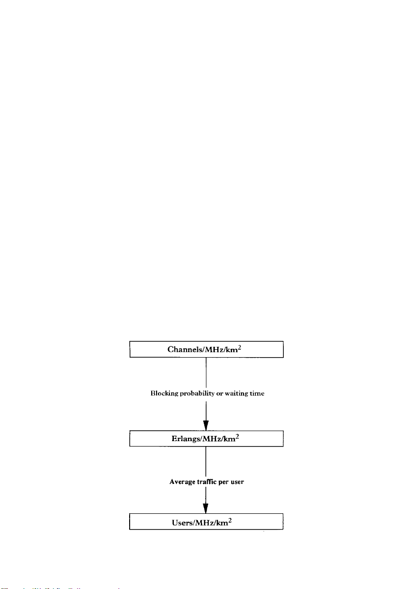
The spectral efficiency measure in Channels/MHz/km
related to the previous measure in Erlangs/MHz/km
sion from Channels/MHz/km

2

to E/MHz/km2is readily obtained

2

is directly

2

. The conver-

given an equivalent blocking probability or waiting time on the voice
channels, when the service is required (Figure 2.1), depending on the
traffic model used.
Another alternative measure of spectral efficiency for cellular systems
is:

2

Users/MHz/km

.

Figure 2.1 Best Measures of Spectral Efficiency in Cellular Systems

16 SPECTRAL EFFICIENCY IN CELLULAR LAND MOBILE RADIO SYSTEMS

It measures the efficiency of a cellular system in terms of the
number of users per MHz of bandwidth allocated for the service in
a unit area.

Unlike the way the term `user' in the above measure is commonly
used, it is intended to be used in such a way that traffic considerations
are included in the measure. To achieve this, the `user' is defined in
terms of the average traffic which he or she generates in a given
cellular system. Consequently, the spectral efficiency measure in
terms of Users/MHz/km
of E/MHz/km

2

(Figure 2.1). To give an example, if the spectral
efficiency of a cellular system is 5 E/MHz/km
generated per user in the system is say 0.05 E, then the efficiency of
that cellular system is 100 Users/MHz/km

2

is directly related to the measure in terms

2

and the average traffic

2

.

2.5 A POSSIBLE SPECTRAL EFFICIENCY MEASURE FOR

DIGITAL SYSTEMS

Digital cellular land mobile radio systems are becoming increasingly
popular. In fact, various digital cellular systems are being proposed
and some deployed in Europe [2.1, 2.8], North America [2.9] and
Japan [2.10]. In a digital modulation system, the voice channel is
defined in terms of kbits/s (kbps). The bandwidth efficiency of a
digital modulation system can be described in terms of bps/Hz.
This latter parameter can be extended to arrive at the following new
spectral efficiency measure for digital cellular systems:

kbps/MHz/km

2

.

According to this new spectral efficiency measure, the more kbps per
MHz a digital system can provide in a unit service area, the more
spectrally efficient it is considered to be. In the following, the advant­ages, disadvantages and limitations of the above spectral efficiency
measure are discussed in comparison with the best spectral efficiency
measures in the previous section:

(a) The spectral efficiency measure in terms of kbps/MHz/km

2

attractive to use with digital cellular systems, although it is not parti­cularly useful for analogue systems. On the other hand, the measure
in terms of Channels/MHz/km

2

is equally applicable to both analo­gue and digital cellular systems, since a voice channel has a definite
meaning whether it is analogue or digitized. Also, the measure in

is

MEASURES OF SPECTRAL EFFICIENCY AND QUALITY CELLULAR SYSTEMS 17

terms of E/MHz/km2is superior to that in terms of kbps/MHz/km
because the former is equally applicable to both analogue and digital
cellular systems. Furthermore, the amount of traffic (in Erlangs)
which can be carried by a group of analogue voice channels is no
different from the traffic which can be carried by the same number of
digitized voice channels.

2

(b) The measure in terms of kbps/MHz/km
the channel spacing or the digitized channel bit rate. This is due to the
fact that the measure kbps/MHz/km

2

was constructed using the

does not account for

spectral efficiency of a digital system in bps/Hz without considering
the bit rate of the digitized channel in kbps. In this case, the spectral
efficiencies of the same digital system employing two different digit­ized voice channels bit rates will falsely appear to be identical. To give
an example, if a cellular system employs a digital modulation techni­que with a spectral efficiency of say 2 bps/Hz and uses a channel bit
rate of 16 kbps and another cellular system employs the same digital
modulation technique but uses a different channel bit rate of say 32
kbps, then the spectral efficiencies of the two cellular systems in terms
of kbps/MHz/km

2

will be identical. Nevertheless, considering the
channel bit rate in kbps, it is obvious that the former digital cellular
system can be twice as spectrally efficient as the latter. In fact, the
spectral efficiency of a digital cellular system in terms of kbps/MHz/

2

km

can be presented in terms of Channels/MHz/km2if coupled

with the bit rate of the digitized voice channel in kbps.

For the above reasons, measures in terms of Channels/MHz/km
E/MHz/km
hensive than the measure in kbps/MHz/km
kbps/MHz/km

2

and Users/MHz/km2are superior and more compre-

2

is useful to use with data-based cellular services

2

. Indeed, the measure

such as telex and facsimile.

2

2

,

2.6 MEASURES OF SPECTRAL EFFICIENCY AND THE

QUALITY OF CELLULAR SYSTEMS

From the previous analysis, the best measures of spectral efficiency
for cellular land mobile radio systems are:

. Channels/MHz/km

. Erlangs/MHz/km

. Users/MHz/km

2

2

2

MeasuresofSpectral Efficiencyand Quality CellularSystems

18 SPECTRAL EFFICIENCY IN CELLULAR LAND MOBILE RADIO SYSTEMS

The above spectral efficiency measures prove to be adequate, com­prehensive and appropriate for cellular systems. For these spectral
efficiency measures to be completely successful, the quality of service
offered by different cellular systems has to be included. However,
when we talk about quality in terms of cellular land mobile radio
systems, typically, the following three kinds of quality requirements
are considered [2.11]:

(a) The degree of coverage in terms of traffic or area. That is to say,
the percentage of the total area in which the service is available.

(b) The grade of service in terms of blocking probability or waiting
time, when the service is required.

(c) The interference levels within the cellular system. This is judged
by the protection ratio of a given modulation technique employed by
the cellular system, which gives rise to a particular voice quality.

Of the above three quality requirements, only (b) and (c) are relevant
to our spectral efficiency measures. Quality in terms of the grade of
service directly applies to the spectral efficiency measures in Erlangs/
MHz/km

2

and Users/MHz/km2since these include traffic considera­tions which are functions of the blocking probability or waiting time,
when the service is required. On the other hand, the voice quality
requirement is applicable to the measure in Channels/MHz/km
since the number of channels obtainable per MHz is limited by the
voice quality offered to the users of the system (i.e. the number of
channels per MHz should not be increased at the expense of voice
quality). However, since the above spectral efficiency measures are
interrelated (Figure 2.1), it can be deduced that the quality in terms of
both the grade of service and voice quality apply to all of our candid­ate spectral efficiency measures. In general, the grade of service and
voice quality can be fixed to a given standard which all mobile radio
systems in comparison have to comply with, and hence, a uniform
quality is maintained throughout the comparison.

2

,

REFERENCES REFERENCES

[2.1] Maloberti, A., 1987 `Definition of the Radio Subsystem for the GSM

Pan-European Digital Mobile Communications System', Proc. International

Conference on Digital Land Mobile Radio Communications Venice, 30 June ± 3
July 1987 pp. 37±47

REFERENCES 19

[2.2] Callender, M., 1987 `Future Public Land Mobile Telecommunication

Systems ± A North American Perspective' Proc International Conference on

Digital Land Mobile Radio Communications, Venice, 30 June ± 3 July 1987

pp. 73±83

[2.3] Hatfield, D. N., 1977 `Measures of Spectral Efficiency in Land Mobile

Radio' IEEE Trans. Electromag. Compat. EMC±19 August pp. 266±8

[2.4] Lane, R. N., 1973 `Spectral and Economic Efficiencies of Land Mobile

Radio Systems' IEEE Trans. Veh. Technol. VT±22, (4) November pp. 93±103

[2.5] Cooper, G. R., 1983 `Cellular Mobile Technology: The Great Multi-

plier', IEEE Spectrum, June pp. 30±7

[2.6] Matthews, P. A. and Rashidzadeh, B., 1986 `A Comparative Study of

Wideband TDMA and TD/FDMA Systems for Digital Cellular Mobile
Radio', Second Nordic Seminar on Digital Land Mobile Radio Communications,
14±16 October 1986 pp. 291±5

[2.7] Bear, D., 1980 `Principles of Telecommunications ± Traffic Engineering'

IEE Telecommunications Series 2

[2.8] Eckert, K. D., 1987 `Conception and Performance of the Cellular Digital

Mobile Radio Communication System CD 900' 37th IEEE Vehicular Techno-
logy Conference, Tampa, Florida, 1±3 June 1987 pp. 369±77

[2.9] Tarallo, J. A. and Zysman, G. I., 1987 `A Digital Narrow-Band Cellular

System' 37th IEEE Vehicular Technology Conference Tampa, Floridag 1±3 June
1987 pp. 279±80

[2.10] Akaiwa, Y. and Nagata, Y., 1987 `Highly Efficient Digital Mobile

Communications with a Linear Modulation Method' IEEE J. Sel. Areas
Commun. SAC±5, (5) June pp. 890±5

[2.11] Gamst, A., 1987 `Remarks on Radio Network Planning' 37th IEEE

Vehicular Technology Conference, Tampa, Florida, 1±3 June 1987 pp. 160±5

3

Spectral Efficiency of
Analogue Modulation
Techniques

3.1 INTRODUCTION Introduction

In the previous chapter, various measures of spectral efficiency in
cellular land mobile radio systems were discussed and possible
measures of spectral efficiency measures were presented. The most
appropriate measures of spectral efficiency for cellular systems are:

. Channels/MHz/km

. Erlangs/MHz/km

. Users/MHz/km

These spectral efficiency measures prove to be adequate, compre­hensive and appropriate for cellular systems. Also, they include the
quality of service offered by different cellular systems in terms of both
voice quality and grade of service. Nevertheless, these spectral effi­ciency measures need to be mathematically interpreted to be able to
calculate the spectral efficiency of various cellular systems. In cellular
land mobile radio systems, there are two major parameters which
govern the spectral efficiency: the modulation technique employed
and the multiple access technique used to trunk the signals in the
system. For the sake of convenience as well as flexibility, we propose
to calculate the efficiency of the modulation technique and the effici­ency of multiple access of a given cellular system in isolation. The
overall spectral efficiency of a particular land mobile radio system is

2

2

2

SPECTRALEFFICIENCYOF ANALOGUEMODULATION TECHNIQUES

21

22 SPECTRAL EFFICIENCY OF ANALOGUE MODULATION TECHNIQUES

then obtained by combining the two types of efficiency due to the
modulation technique employed and the multiple access technique
used in conjunction.

The main purpose of this chapter is to devise a criterion by
which the spectral efficiency of various analogue modulation tech­niques can be evaluated, when employed in cellular systems. To
aid this objective, it is necessary to have an overview of the basic
analogue modulation techniques, with particular emphasis on the
prime parameters which determine the efficiency of a modulation
technique. The spectral efficiency measure in terms of Channels/
MHz/km

2

is then mathematically interpreted and the efficiency of
a cellular system employing a particular modulation technique is
presented as a function of channel spacing, number of cells per cluster
and cell area.

The concept of cellular geometry is also introduced in order to
relate the number of cells per cluster to the co-channel re-use ratio,
and hence the spectral efficiency due to a modulation technique is
given in terms of the channel spacing, co-channel re-use ratio and the
cell area. It is of great importance, however, to relate the spectral
efficiency of modulation techniques to speech quality experienced
by the users in the cellular system. The speech quality, in turn, is
influenced by the signal to co-channel protection ratio determined by
the modulation technique used. To establish a relationship between
the protection ratio and the co-channel re-use ratio, it is necessary to
model the cellular land mobile radio environment in such a way that
propagation effects on the radio signal are accounted for. It is also
necessary to model the relative geographical locations of the transmit­ters and the receivers in the system so as to be able to predict all the
significant co-channel interference affecting the desired signal. For
this purpose, a thorough comparative study of six different models
is conducted and the best model of all is used. The modulation
efficiency is given in terms of channel spacing, protection ratio, pro­pagation constant and cell area.

3.2 BASIC ANALOGUE MODULATION TECHNIQUES BasicAnalogueModulation Techniques

All information-bearing signals must ultimately be transmitted over
some intervening medium (channel) separating the transmitter and
the receiver. In the case of land mobile radio communications, this
medium is free space. Modulation is the process whereby signals
which naturally occur in a given frequency band, known as the

BASIC ANALOGUE MODULATION TECHNIQUES 23

baseband, are translated into another frequency band so that they can
be matched to the characteristics of the transmission medium [3.1].
Thus, for example, electrical signals created by a human voice need to
be translated into the radio frequency (RF) spectrum before they can
be translated for radio communication purposes. They then have to be
transmitted back into the baseband, by a complementary process
known as demodulation before they can be used to reproduce the
signals which are audible to the recipient. Also, modulation is the
process of transferring information to a carrier, and the reverse opera­tion of extracting the information-bearing signal from the modulated
carrier is called demodulation [3.2].

The information to be transmitted is contained in the baseband
signal; however, it is not feasible to transmit it in this form and
modulation is required for the following reasons

(a) To match the signal to the frequency characteristics of the trans­mission medium, as mentioned before.

(b) For the ease of radiation. If the communication channel consists
of free space, such as in land mobile radio, then antennas are neces­sary to radiate and receive the signal. For efficient electromagnetic
radiation, antennas need to have physical dimensions of the same
order of magnitude as the wavelength of the radiated signal. Voice
signals, for example, have frequency components down to 300 Hz.
Hence, antennas some 100 km long would be necessary if the signal is
radiated directly. If modulation is used to impress the voice signal on
a high-frequency carrier, say 900 MHz, then antennas need be no
longer than ten centimetres or so.

(c) To overcome equipment complexity. Modulation can be used for
translating the signal to a location in the frequency domain where
design requirements of signal processing devices (e.g. filters and
amplifiers) are easily met.

(d) To reduce noise and interference. It is possible to minimize the
effect of noise in communication systems by using certain types of
modulation techniques. These techniques generally trade bandwidth
for noise reduction and thus require a transmission bandwidth much
larger than the bandwidth of the baseband signal.

(e) For multiplexing. Land mobile radio systems are mainly used
for voice transmission (telephony). A band-limited voice signal
has components between 300 Hz and 3 kHz, thus, modulation

24 SPECTRAL EFFICIENCY OF ANALOGUE MODULATION TECHNIQUES

is used to translate different baseband signals to different spectral
locations to enable different receivers to select the desired voice
channel.

(f) For frequency assignment. In land mobile radio systems, the use
of modulation allows several hundreds of users to transmit and
receive simultaneously at different carrier frequencies, using the
same radio frequency band. This kind of need for modulation and
the previous case (e) are grouped under the multiple access tech­niques, and hence their efficiencies will not be considered in this
chapter.

In analogue modulation, a parameter of a continuous high-frequency
carrier is varied in proportion to a low-frequency baseband message
signal. The carrier to be modulated is usually sinusoidal and has the
following general mathematical form:

x

tvt cos wct  t wc 2 f

c

c

3:1

where vt is the instantaneous amplitude of the carrier, f

is the

c

carrier frequency and t is the instantaneous phase deviation of
the carrier.

The carrier can be modulated by varying one of the above para­meters in accordance with the amplitude of the baseband message
signal.

In principle, all analogue modulation techniques fall into two major
categories: linear or amplitude modulation techniques and non-linear
or angle modulation techniques. If vt is linearly related to the mes­sage signal mt, then we have linear or amplitude modulation. If t
or its time derivative is linearly related to mt, then we have angle
modulation, which is a non-linear modulation. The following is an
overview of basic analogue modulation techniques, paying particular
attention to three important parameters. These parameters are: the
transmission bandwidth, the transmitted power and the average sig­nal to noise power ratio performance of each modulation technique.
Whenever possible, the message signal m(t) will be taken as a band­limited voice signal, normalized such that 1  mt1 and having
frequency components between 300 Hz and 3 kHz. The noise at the
input to the receiver is considered to be additive white Gaussian noise
(AWGN). Furthermore, for the signal to noise ratio comparisons, all
modulation systems will be assumed to operate with the same aver­age transmitted power.

BASIC ANALOGUE MODULATION TECHNIQUES 25

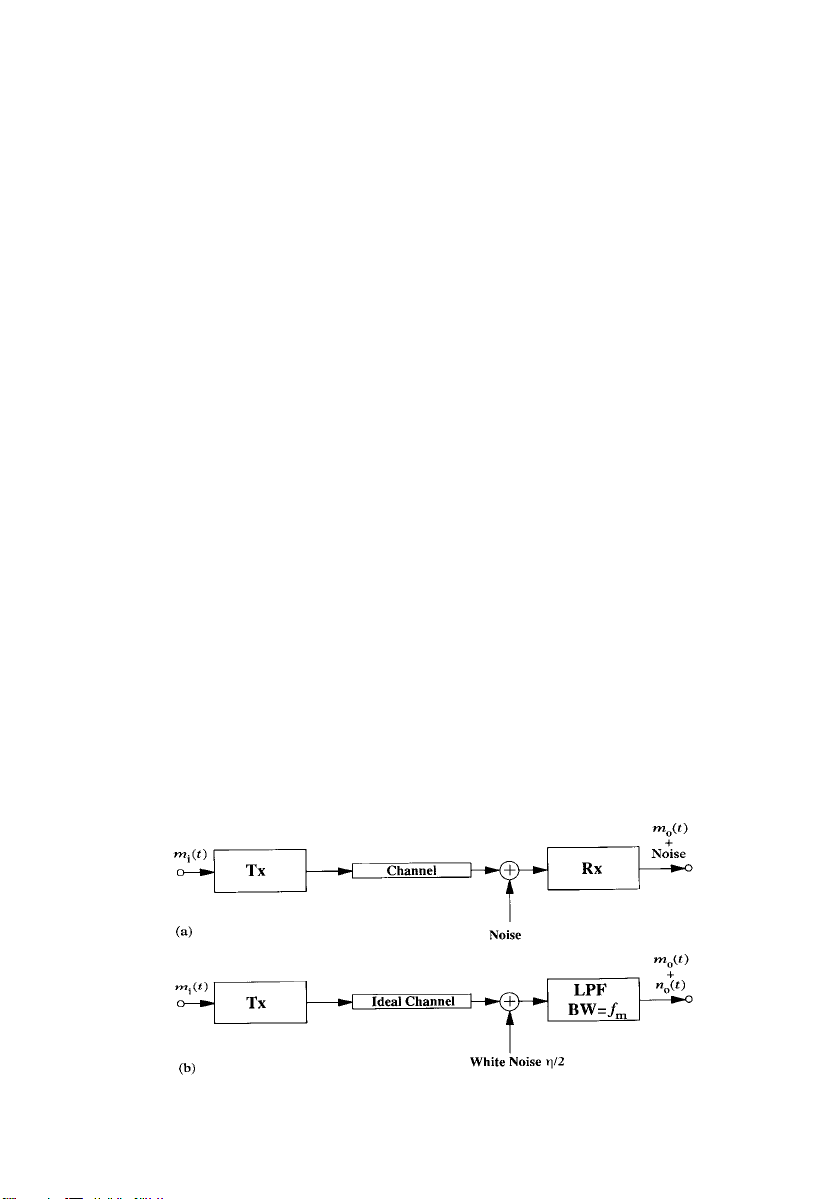
3.2.1 Analogue Baseband Signal Transmission

Baseband systems are communication systems in which signal trans­mission takes place without modulation. They are useful as a basis for
the comparison of various analogue modulation techniques. Figure

3.1(a) shows a typical block diagram of a baseband communication
system, where signal power amplification and necessary filtering are
performed by the transmitter and the receiver. No modulation or
demodulation is performed and the message signal is modified at
the output by the non-ideal characteristics of the channel and the
addition of noise in the system. If the baseband system is to be
distortionless, then the message signal at the output should satisfy
the following equation:

m

tkmit  td3:2

o

where m

t is the input message signal, mot is the output message

i

signal, k is constant representing the attenuation caused by the chan­nel and t

is a constant representing the time delay caused by the

d

channel.

From Equation (3.2), it is clear that for distortionless transmission,
the message is simply attenuated and delayed in time, and hence the
content of the message is unaltered. Nevertheless, some distortion
will always occur in signal transmission, and three common types of
distortion can be identified as follows:

(a) Amplitude distortion which occurs when the amplitude
response of the channel over the range of frequencies for the input

Figure 3.1 Baseband Communication System. Tx, Transmitter; Rx, Receiver. (a)
Distortionless System. (b) Baseband System and White Noise

26 SPECTRAL EFFICIENCY OF ANALOGUE MODULATION TECHNIQUES

signal is not flat. In this case, different spectral components of the
input message are attenuated differently. The attenuation shown in
Equation (3.2) will not be constant but will be a function of frequency
kf . The most common forms of amplitude distortion are excess
attenuation of high or low frequencies in the signal spectrum and it
is worse for wideband signals.

(b) Phase or delay distortion which occurs when different frequency
components of the input message signal suffer different amounts of
time delay. In this case, the time delay in Equation (3.2) is not constant
but a function of frequency t

f. For voice transmission, delay dis-

d

tortion is not a problem since the human ear is insensitive to this type
of distortion.

(c) Non-linear distortion due to the presence of non-linear elements
in the channel such as amplifiers. Non-linear elements have transfer
characteristics which act linearly when the input signal is small, but
distort the signal when the input amplitude is large. Mathematically,
the non-linear device can be modelled by:

where k

m

tk1mitk2m

o

, k2, k3; ..., are constants. To demonstrate the effect of non-

1

2

tk3m

i

3

t... 3:3

i

linear distortion, consider the input to be the sum of two cosine
signals with frequencies f
harmonic distortion terms at frequencies 2 f
distortion terms at frequencies f

and f2. In this case, the output will contain

1

,2f2and intermodulation

1

 f2,2f1 f2,2f2 f1, etc. This prob-

1

lem is of great concern in systems where a number of different
message signals are multiplexed together and transmitted over the
same channel.

The types of distortion mentioned in (a) and (b) above are called linear
distortion and can be cured by the use of equalizers which are essen­tially designed to compensate for the different attenuation and delay
levels of the signal at different frequency components. The non-linear
distortion mentioned in (c) can be reduced using companders which
compress the signal prior to transmission for its amplitude to fall
within the linear range of the channel. Then, the signal at the receiver
is expanded to restore its appropriate level. Companding is widely
used in telephone systems to reduce non-linear distortion and also to
compensate for signal levels which differ between soft and loud
talkers.

BASIC ANALOGUE MODULATION TECHNIQUES 27

Signal to noise performance of baseband systems

The signal quality at the output of an analogue modulation system is
usually measured in terms of the average signal power to noise
power, defined as:

2

Efm

tg

S9=N

Efn

o

2
o

tg



o

3:4

where m

t is the output signal message, not is the noise at the

o

output of the system and Efxg denotes the average of x.

The message signal will be taken as a voice signal, band-limited to

f

and hence satisfies the condition:

m

M

where M

f 0 for f  fmand f f

o

f is the Fourier transform of mot.

o

m

3:5

Since our objective is the comparison of various analogue
modulation techniques in terms of their signal to noise ratio (SNR)
performance, it suffices to consider the special case of an ideal channel
with additive white noise with a power spectral density (psd) of =2
W/Hz (see Figure 3.1(b) ). Also, assuming ideal filters, in the case of a
baseband system, a lowpass filter with cut-off frequency f
at the receiver. Now, if Efm
power P

at the output, then:

R

S=N

2

tg is the recovered average signal

o

P

R



o

 say3:6

 f

m

is needed

m

Hence:

S=N

received signal power



o

in-band noise power

: 3:7

If the channel is not ideal but distortionless, then using Equation (3.2),
the signal to noise power ratio can be presented in terms of trans­mitted signal power P

at the input to the system:

T

P

2

S=N

o

 k

T

: 3:8

 f

m

In general, the signal to noise power ratio given in Equation (3.8) is
considered to be an upper limit for practical analogue baseband
performance. The signal to noise ratios shown in Equations (3.6) and

28

SPECTRAL EFFICIENCY OF ANALOGUE MODULATION TECHNIQUES

(3.8) will be taken as a basis to compare the performance of various
modulation techniques.

3.2.2 Double-Sideband (DSB) Modulation

This is probably the simplest form of linear or amplitude modulation.
It is achieved by multiplying the message signal mt by a high­frequency carrier x

t as shown in Figure 3.2(a), where:

c

tcos wct: 3:9

x

c

For simplicity, the phase of the carrier is dropped and the amplitude
is made equal to unity, since this will not affect the generality of the
analysis. The modulated message signal is hence given by:

xtmt cos w

t3:10

c

"#

A

y

1

Xf

2

Mf f

B

Mf fc 3:11

c

Figure 3.2 (a) DSB Modulator. (b) DSB Modulation in the Frequency Domain

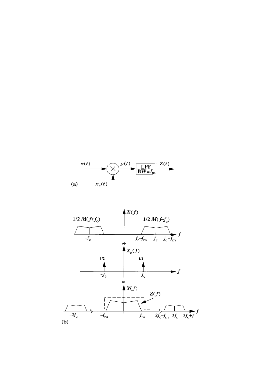
BASIC ANALOGUE MODULATION TECHNIQUES 29

where Xf  and Mf are the Fourier transforms of xt and mt
respectively.

The result is graphically represented in Figure 3.2(b) in the fre­quency domain. Using this type of modulation simply translates the
spectrum of the baseband message signal to the carrier frequency.
This is called double-sideband suppressed carrier (DSB-SC) modula­tion, since there is no carrier term in the modulated signal.

Demodulation of DSB signals

To demodulate a DSB signal, it is multiplied by a carrier replica and
then the resultant is passed through a lowpass filter as shown in
Figure 3.3(a). The spectrum of the demodulated signal before and
after filtering is shown in Figure 3.3(b). Assuming an ideal channel,
Yf is given by:

Figure 3.3 (a) DSB Demodulator. (b) DSB Demodulation in the Frequency
Domain

30 SPECTRAL EFFICIENCY OF ANALOGUE MODULATION TECHNIQUES

Yf

1

Mf 

2

1

Mf 2 f

4

Mf 2 fc: 3:12

c

After lowpass filtering:

1

Zf 

; zt

Mf 3:13

2
1

mt: 3:14

2

The message signal mt is hence fully recovered provided that:

f

> fm:

c

The demodulation scheme used above is called synchronous or coher­ent demodulation. It requires a local oscillator at the receiver which is
precisely synchronous with the carrier signal used to demodulate the
message signal. This is a very stringent condition which cannot be
satisfied easily in practice. There are other demodulation techniques
that are used to generate a coherent carrier and these are described in
[3.2] and [3.3].

Transmitted signal power and bandwidth of DSB signals

From Figure 3.2(b), it can be seen that the bandwidth BTrequired to
transmit a message signal of bandwidth f

B

 2 fm: 3:15

T

using DSB-SC is:

m

It is obvious that this is a waste of spectrum since both sidebands of the
signal are transmitted, yet they carry identical information.

The average transmitted power P

of the DSB modulated signal xt

T

is given by:

P

 Efx2tg Assuming 1 load3:16

T

P

 Efm2t cos2wctg 3:17

T

1

P



T

m

2

3:18

where P

; P

is the average message signal power.

m

BASIC ANALOGUE MODULATION TECHNIQUES 31

Signal to noise performance of DSB-SC systems

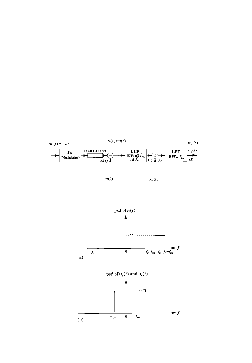
To find the signal to noise performance of a DSB-SC modulation
system, consider the model depicted in Figure 3.4, with ideal channel
and ideal subsystems. The signal is assumed to be corrupted with
additive white Gaussian noise (AWGN) nt, with the following quad­rature representation [3.4]:

ntn

t cos wctnst sin wct3:19

c

where nt is the Narrowband or bandpass AWGN, n
phase, lowpass AWGN component and n

t is the quadrature, low-

s

pass AWGN component.

The psds of nt, n

Figure 3.4 Model of DSB Modulation System Corrupted with AWGN

t and nst are shown in Figure 3.5.

c

t is the in-

c

Figure 3.5 (a) Bandpass AWGN Representation. (b) Lowpass AWGN Represent­ation

32 SPECTRAL EFFICIENCY OF ANALOGUE MODULATION TECHNIQUES

The bandpass filter shown in Figure 3.4 (also referred to as the pre­detection filter) is used to remove the out of band noise and any
harmonic signal terms. At point (1) in figure 3.4, the DSB signal plus
noise is given by:

mt cos w

tnct cos wctnst sin wct: 3:20

c

At point (2), the DSB signal plus noise is multiplied by a synchronous
replica of the carrier signal. The resultant is given by:

mt cos2wctnct cos2wctnst sin wct cos wct3:21

1

mtf1  cos 2w



2

tg 

c

1

n

tf1  cos 2wctg 

c

2

1

n

t sin 2wct: 3:22

s

2

At point (3), the double-frequency terms are removed by the lowpass
filter (also referred to as the post-detection filter), and the output will
be:

1

mt

2

1

n

tmotnot: 3:23

c

2

Using the definition of the average signal to noise power ratio in
Equation (3.4):

1

Ef

m2tg

S=N

S=N

2

Efn

tg   B

c

; S=N



o



o

 2 f



o

4

1

2

Ef

n

tg

c

4

Efm2tg

2

Efn

tg

c

T

m

P

m

: 3:27

2 f

m

3:24

3:25

3:26

But:

1

P

2

; S=N

 Efm2t cos2wctg  P

m

P

R



o

 : 3:39

 f

m

R

3:28

For a distortionless channel, the signal to noise ratio is given in terms
of the transmitted power, hence:

BASIC ANALOGUE MODULATION TECHNIQUES 33

k2P

; S=No

T

 : 3:30

 f

m

Therefore, the signal to noise power ratio for DSB-SC systems is
identical to that for analogue baseband transmission.

3.2.3 Amplitude Modulation (AM)

This is another type of linear modulation which can be generated by
adding a large carrier component to a DSB signal. The amplitude
modulated signal has the following form:

xt1  mt cos w

xtcos w

tmt cos wct3:32

c

t3:31

c

; AM  carrier DSB-SC: 3:33

It can be seen that the envelope of the AM signal resembles the
message signal provided that the following conditions are met:

f

c

 f

m

and 1  mt > 0:

An important parameter of an amplitude modulated signal is the
modulation index m

defined as:

x

peak DSB-SC amplitude

m



x

peak carrier amplitude

: 3:34

Hence, a more general form of an amplitude modulated signal is:

xt1  m

mt cos wct: 3:35

x

The message signal can be completely recovered from the AM signal
by simply using an envelope detector provided that m
exceed one. If m

does exceed one, then the carrier is said to be

x

does not

x

overmodulated, which results in envelope distortion and hence envel­ope detection is not possible in this case.

Transmitted signal power and bandwidth of AM signals

The transmission bandwidth of an AM signal is the same as that for a
DSB-SC:

34 SPECTRAL EFFICIENCY OF ANALOGUE MODULATION TECHNIQUES

BT 2 fm:

Using Equation (3.32), the average transmitted power P

of an AM

T

signal is:

1

 Pc

P

T

where P

is the average carrier signal power.

c

For a sinusoidal carrier with unity amplitude, P

P

: 3:36

m

2

equals a half and

c

the average transmitted power is hence given by:

1

1





P

T

P

: 3:37

2

m

2

The power efficiency of an AM signal is given by the ratio of the
power which is used to convey information (i.e. the message signal) to
the total transmitted power, hence:

1

P

m

power efficiency 



2

1



2

P

m

1  P

1

P

m

2

: 3:39

m

3:38

A more general expression for the power efficiency includes the
modulation index m

:

x

2

m

P

m

Power Efficiency   

x

1  m

: 3:40

2

P

m

x

It can be shown that the maximum power efficiency is achieved when
the modulation index m

is one. For an arbitrary message signal (e.g. a

x

voice signal), the maximum power efficiency is 50% and for a sine
wave message signal the maximum power efficiency is 33.3%. We can
conclude that AM is power inefficient due to the power P

expended

c

in the carrier. Nevertheless, this carrier power is vital for simple
amplitude demodulation.

Signal to noise performance of AM systems

The signal to noise performance of AM systems can be derived in
a similar fashion as for DSB systems. Only the result is given for

BASIC ANALOGUE MODULATION TECHNIQUES 35

envelope detection (non-coherent modulation) of an AM signal, with
the assumption that the signal power at the receiver input is much
higher than the inband noise power. The average signal to noise ratio
at the output of the receiver is then given by [3.2]:

P

S=N

; S=N

R



o

  3:42

o

 3:41

 f

m

where  is the power efficiency of the AM signal as given by Equation
(3.40) and  is the equivalent average signal to noise power ratio for
analogue baseband transmission. For 100% modulation (i.e. m

x

 1)

and an arbitrary message signal, the maximum value for  is a half.
Hence, the average signal to noise ratio for an AM system is:

1

 3:43

S=N



o

2

which is at least 3 dB poorer than for baseband transmission and for
DSB-SC modulation.

3.2.4 Single-Sideband (SSB) Modulation

In cellular land mobile radio systems, it is essential that the modula­tion techniques employed are spectrally efficient. It can be seen from
the previous sections that DSB-SC and AM techniques are both waste­ful in terms of spectrum since the transmission bandwidth is twice
that of the message signal. Furthermore, AM techniques are also
wasteful in terms of transmitted power and have a poor signal to
noise performance compared with DSB-SC techniques. In SSB mod­ulation, only one of the two sidebands which result in multiplying the
message signal mt with the carrier is transmitted. Conceptually, the
simplest way of generating a SSB signal is to first generate a DSB
signal and then suppress one of the sidebands using a bandpass filter.
Coherent demodulation of a SSB signal is possible using a synchron­ous carrier, in the same way as for a DSB signal.

Modulation and demodulation of SSB signals as described above
seem to be simple and straightforward, however, practical implemen­tation of the SSB technique is not trivial for two reasons. First, the
modulator needs an ideal bandpass sideband filter with sharp cut-off
characteristics which cannot be exactly achieved in practice. Second,

36 SPECTRAL EFFICIENCY OF ANALOGUE MODULATION TECHNIQUES

coherent demodulation requires a carrier reference at the receiver
which is precisely synchronous with the carrier signal used to generate
the modulated message signal. Voice message signals do not contain
significant low-frequency components. Consequently, there will be no
significant frequency components in the vicinity of the carrier fre­quency f

after modulation and hence the use of `brickwall' sideband

c

filtering is not really necessary. Alternatively, SSB signals can be gen­erated by a proper phase shifting of the message signal, which does not
require a sideband filter. Envelope detection of SSB signals can be
employed instead of synchronous demodulation by adding a carrier
frequency component to the SSB signal at the transmitter, in the same
way described for AM. Nevertheless, this will lead to a waste of
transmitted power and to an inferior signal to noise performance.

Transmitted signal power and bandwidth of SSB signals

The bandwidth BTrequired to transmit a message signal of band­width fm using SSB modulation is:

 fm: 3:44

B

T

The average transmitted power P

of a SSB modulated signal can be

T

easily verified to be half that of a SSB-SC signal, provided that the
average message signal power is identical in both cases. That is, for a
SSB:

1

P

P



T

: 3:45

m

4

Signal to noise performance of SSB systems

For coherent demodulation of SSB signals, the average signal to noise
performance can be derived in the same way as for DSB-SC signals.
The average signal to noise ratio at the output of the receiver is given
by [3.2]:

P

S=N

Equation (3.46) indicates that S=N

R



o

 : 3:46

 f

m

for SSB systems is identical to

o

that for baseband and DSB-SC systems, in the presence of white noise.

BASIC ANALOGUE MODULATION TECHNIQUES 37

3.2.5 Angle (Non-linear) Modulation

In contrast to the linear modulation techniques discussed in the pre­ceding sections, angle modulation is a non-linear process where the
spectral components of the modulated message signal are not related
in any simple fashion to the baseband message signal. Considering
the sinusoidal carrier given by Equation (3.1), and assuming a con­stant amplitude such that vtV

x

tVccos wct  t: 3:47

c

:

c

Angle modulation is achieved by relating t or its derivative to the
message signal mt, while keeping the amplitude of the carrier V
constant (for convenience, let Vc 1). Hence, an angle modulated
signal will have the following general form:

c

xtcos w

t  f mt: 3:48

c

The relation between t and mt can take any mathematical
form which can lead to many types of angle modulation techniques.
However, only two types of angle modulation techniques have
proved to be practical: phase modulation (PM) and frequency mod­ulation (FM). In PM, t is linearly related to the message signal mt
and in FM the time derivative of t is linearly related to mt.
Mathematically:

tk

d=d

where t is the instantaneous phase deviation of xt,d=d
instantaneous frequency deviation of xt, k
constant, expressed in rad/V and, k

mt for PM 3:49

p

 kfmt for FM 3:50

t

is the

t

is the phase deviation

p

is the frequency deviation con-

f

stant, expressed in rad/s/V.

Hence, an angle modulated signal can be expressed in the following
forms:

xtcos w

xtcos w

t  kpmt for PM 3:51

c

Z

t

t  k

c

mudu for FM: 3:52

f

0

38 SPECTRAL EFFICIENCY OF ANALOGUE MODULATION TECHNIQUES

Transmitted signal power and bandwidth of FM signals

The spectrum of an angle modulated signal for an arbitrary message
signal is difficult to describe because of the non-linearity of the angle
modulation process. Instead, the spectra for a frequency modulated
sinusoidal message signal is usually examined and the result is then
generalized for arbitrary message signals. Giving the result only, the
bandwidth B

required to transmit a message signal of bandwidth f

T

using FM modulation is [3.2]:

 2  1 fm: 3:53

B

T

The above expression is referred to as Carson's rule and  is defined
as follows:

m

peak frequency deviation

 

message signalbandwith

f





: 3:54

f

m

The peak frequency deviation is given by Equation (3.50), when the
absolute value of mt is maximum. Based on the value of ,FM
signals fall into two categories as follows.

a For   1; B

 2 fm: 3:55

T

This is called narrowband FM (NBFM), and the transmission band­width in this case is the same as for DSB and AM. NBFM modulation
has no inherent advantages over linear modulation techniques.

b For   1; B

 2 fm 2 f: 3:56

T

In this case, the FM signal is called a wideband FM (WBFM) signal.
It is obvious that the transmission bandwidth of a WBFM signal is
much larger than f

and is dependent upon the value of  (or f).

m

From equation (3.52), the average normalized transmitted power of
the FM modulated signal mt is:

P

 Efx2tg

T

1

P

:



T

2

3:57

Hence, the average transmitted power of a frequency modulated
signal is a function of the amplitude of the carrier signal and is

BASIC ANALOGUE MODULATION TECHNIQUES 39

independent of the message signal mt. This is an expected result
since the message signal causes only the `angle' of the carrier to
change without altering its amplitude.

Signal to noise performance of FM systems

The signal to noise ratio of a FM system is taken as the ratio of the
mean signal power without noise to the mean noise power in the
presence of an unmodulated carrier. Hence, assuming that the output
noise power can be calculated independently of the modulating signal
power yields the following result [3.2]:

S=N

 32Pm: 3:58

o

The above expression is valid provided that the signal power at the
receiver (detector) is much higher than the noise power. This is
referred to as the threshold effect of FM systems, below which the
signal to noise performance of the FM system deteriorates markedly.
From Equation (3.58), it is obvious that S=N
increasing  (or f

), without having to increase the transmitted power.



Increasing  will increase the transmission bandwidth B

can be increased by

o

as shown in

T

Equation (3.56). Thus, in WBFM systems, it is possible to trade off
bandwidth for improved signal to noise performance without having
to increase the transmitted signal power, provided that the system is
operating above threshold.

3.2.6 General Comparison of Various Analogue Modulation
Techniques

In the previous section, an overview of the basic analogue modulation
techniques was presented. A general comparison of the various
analogue modulation techniques in terms of transmission bandwidth
and the average signal to noise performance is given in Table 3.1. It is
assumed that a normalized voice message signal is used, such that:

1  mt1 and Efm

2

tg  Pm

1

:

2

The transmission bandwidth is vital for spectral efficiency consid­erations and the signal to noise performance reflects the signal quality
at the receiver. Equipment complexity is not considered since spectral

40

SPECTRAL EFFICIENCY OF ANALOGUE MODULATION TECHNIQUES

Table 3.1 General Comparison of Various Analogue Modulation Techniques

Modulation B

Baseband f
DSB-SC 2f
AM 2 f

SSB f

WBFM 2  1 f

NBFM 2 f

T

m

m

m

m

m

S=N

0

 ÐÐ
 Wasteful of bandwidth
 =3 Wasteful of power and bandwidth

 Spectrally efficient and good

3=2 2 Superior S=N0performance but

m

  Same bandwidth as DSB and AM

Suitability to Cellular Systems

and poor S=N

S=N

performance

0

excessive use of bandwidth

but S=N
inferior

0

performance

0

performance is far

efficiency is of prime importance in cellular land mobile radio sys­tems. From Table 3.1, amongst linear modulation techniques, SSB is
both spectrally efficient and has a good signal to noise performance.
On the other hand, FM has a superior signal to noise performance
over all other modulation techniques. However, the excessive use of
bandwidth in FM systems is yet to be justified for cellular systems.
Furthermore, the FM system has a superior signal to noise perfor­mance above threshold but for small signal to noise conditions the FM
system may actually be inferior to other linear modulation techniques.

The above comparison is incomplete and can only show the poten­tial spectral efficiency of various modulation techniques because of
the idealized conditions assumed for their operation. A more realistic
approach is first to establish a rigorous and comprehensive set of
criteria with which the spectral efficiency of various modulation tech­niques can be evaluated in terms of their important parameters. Sec­ond, the spectral efficiency of different modulation techniques should
be considered within the cellular environment. In the following, the
spectral efficiency measure in terms of Channels/MHz/km

2

is used to
devise a method to evaluate the spectral efficiency of various modula­tion techniques when implemented by cellular systems.

3.3 MATHEMATICAL INTERPRETATION OF CHANNELS/

MHZ/KM

2

Consider a cellular land mobile radio system with a service area
divided into a number of clusters of equal area, every cluster is

MathematicalInterpretationof Channels

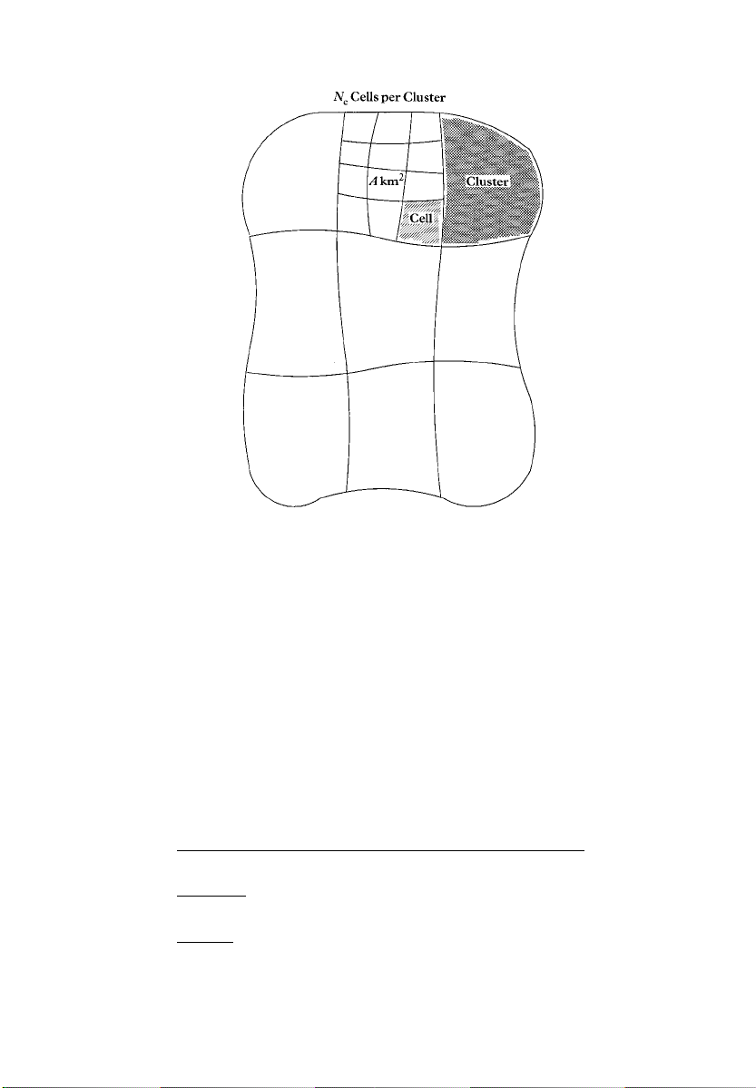
MATHEMATICAL INTERPRETATION OF CHANNELS 41

Figure 3.6 Service Area Divided into Cells and Clusters

sub-divided into Nccells of equal area, each is A km2(see Figure 3.6).
A total bandwidth of B

MHz is assumed to be available to the system

t

and this total bandwidth is divided into voice channels, each is B
MHz in bandwidth. In this case, the number of channels available to
the system is given by B

, and Bcwill be mainly governed by the

t=Bc

modulation technique employed. Adopting the measure of spectral
efficiency in cellular systems as Channels/MHz/km

2

, the spectral
efficiency of a modulation technique can be mathematically inter­preted by the following equations:

total number of channels available to the system





M



M



M

where 





M

total available bandwith  cluster area

Bt=B

c

BtNcA

1

A

B

cNc

is called the modulation efficiency of the cellular system,

expressed in terms of Channels/MHz/km

2

.

3:59

3:60

3:61

c

42 SPECTRAL EFFICIENCY OF ANALOGUE MODULATION TECHNIQUES

From the above equations, we note the following:

(a) For point-to-point and non-cellular radio systems, the spectral
efficiency can be simply presented in terms of the number of channels
available to the system and is given by B

(channels). In such

t=Bc

systems the spectral efficiency is a function of the channel spacing

B

only.

c

(b) In cellular systems, the modulation efficiency measured in Chan-

2

nels/MHz/km

is inversely proportional to the channel spacing Bc.
The modulation efficiency is independent of the total bandwidth B
allocated to the cellular system, excluding multiple access efficiency
considerations.

(c) The spectral efficiency of a cellular system is inversely pro­portional to the cluster area given by N

A. This is because the

c

cluster is the repetition unit in cellular systems and not the cell.
Consequently, the more clusters a cellular system can accommodate
in a given service area, the more spectrally efficient it is considered
to be.

(d) The modulation efficiency 

B

, Ncor A. The channel spacing Bcis dependant on the modulation

c

can be maximized by minimising

M

technique employed by the cellular system. The theoretical minimum
of N
maximum efficiency, as far as N

is one and in this case one cell per cluster will give rise to

c

is concerned. Furthermore, min-

c

imizing the cell area will depend upon several factors such as the
transmitted power, hand-off rate and the availability and tolerance of
cell sites.

3.4 CALCULATION OF THE NUMBER OF CELLS PER

CLUSTER N

c

Calculationofthe Numberof CellsperCluster

t

From the previous section, the spectral efficiency of a modulation
technique within cellular systems is shown to be a function of three
parameters ± channel spacing B
cell area A. It will be shown that N

, number of cells per cluster Ncand

c

is a very important parameter

c

which relates to some parameters of the modulation technique
employed. On the other hand, N

depends on the cell shape as well

c

as the model used to calculate the co-channel interference in the
system.

CALCULATION OF THE NUMBER OF CELLS PER CLUSTER 43

3.4.1 Cellular Geometry

The main reason for defining cells in a cellular land mobile radio
system is to outline areas in which specific channels and specific cell
sites are used. However, designers realize that visualizing all cells as
having the same geometrical shape helps to ease the design of cellular
systems, not only in locating transmitter sites relative to one another
and making economical use of equipment, but it also makes the
adaptation to traffic much easier. From our viewpoint, cellular geo­metry helps to ease the assessment of spectral efficiency of various
cellular systems, in particular to calculate the significant co-channel
interference in the system.

3.4.2 Cell Shapes

There are only certain patterns of cells or tessellations which can be
repeated over a plane: the regular hexagon, the square and the trian­gle. The regular hexagon is favoured by system designers for the
following reasons:

(a) It provides the best approximation to the circular omnidirec-

tional radio patterns achieved in practice.

(b) It is more economical to use, since a hexagonal layout requires

fewer cells and hence fewer base stations.

(c) It combines ease of geometry to the practical realization of over-

lapping circles.

3.4.3 Principles of Hexagonal Geometry

The are several objectives for describing the fundamentals of
hexagonal geometry. First, to outline clusters of cells and calculate
the number of cells per cluster N

in terms of other parameters of

c

the cellular system. Second, to locate co-channel cells and calculate the
co-channel cell separation D in terms of N

. To be able to do this, the

c

co-channel re-use ratio is defined as:

co-channel re-use ratio 

minimum co-channel cell separation

cell radius

D

Q 

: 3:63

R

3:62

44

SPECTRAL EFFICIENCY OF ANALOGUE MODULATION TECHNIQUES

It can be seen that the co-channel interference can be reduced if Q
is made large enough. For this reason, Q is also referred to as the
co-channel interference reduction factor [3.5]. This is an important
and useful factor in cellular land mobile radio systems. For a fixed
cell size, co-channel interference is independent of the transmitted
power of the base station in each cell. In fact, co-channel interference
is a function of Q only, as will be shown later.

Figure 3.7 shows a cellular pattern using regular hexagons and a

convenient set of axes intersecting at 608 [3.6]. Cearly:

R cos 30

1





2

giving R 

1

p

: 3:64

3

To find the distance r of a point Pu; v from the origin and using x±y
to u±v co-ordinates transformations:

2

 x2 y

r

x  u cos 30

2



and



y  v  u sin 30

:

Figure 3.7 Hexagonal Cell Geometry with a Convenient Set of Axes

CALCULATION OF THE NUMBER OF CELLS PER CLUSTER 45

Hence:

r v

2

 uv  u2

1=2

: 3:65

Using Equation (3.65) to locate co-channel cells, we start from a
reference cell and move i hexagons along the u-axis then j hexagons
along the v-axis. Hence, the distance D between co-channel cells in
adjacent clusters is given by:

1=2

: 3:66

The number of cells N

2

D i

in a cluster is proportional to D2, i.e. Nc!D

c

 ij  j2

and it is shown in [3.6] that:

N

; N

 D

c

 i2 ij  j

c

precisely 3:67

2

3:68

2

Since i and j can only take integer values, Equation (3.68) suggests
that N
etc., are possible values of N

can only take particular values, e.g. Nc 1, 3, 4, 7, 9, 12, 13,

c

. In Figure 3.7, the heavy border outlines

c

a cluster of seven cells and the shaded cells are co-channel cells (i.e.
using the same set of voice channels with the same radio frequencies).
In fact, there are precisely six proximate co-channel cells for all values
of N

.

c

Relationship between the co-channel re -use ratio D/R and the number of
cells per cluster N

c

From Equations (3.64) and (3.66):

D=R f3i

2

 ij  j2g

1=2

2

and using Equation (3.68):

D=R p3N

: 3:69

c

Hence, the modulation efficiency is given in terms of D=R as follows:

B

D=R2A

c

3





M

: 3:70

46 SPECTRAL EFFICIENCY OF ANALOGUE MODULATION TECHNIQUES

In practice, co-channel interference considerations influence the

choice of the number of cells per cluster. Making D=R smaller leads
to a spectrally more efficient cellular system, a result confirmed by
Equation (3.70). However, for a better transmission quality in terms of
signal to co-channel interference, D=R needs to be large. A trade off
between the two objectives ± spectral efficiency and transmission
quality ± must be achieved when comparing different modulation
systems in terms of spectral efficiency. Hence, we conclude that to
compare different modulation systems in terms of spectral efficiency,
a certain voice quality standard has to be set and user satisfaction has
to be achieved.

3.5 RELATIONSHIP BETWEEN CO-CHANNEL RE-USE

RATIO AND PROTECTION RATIO IN A CELLULAR
SYSTEM

The spectral efficiency of a cellular land mobile radio system employ­ing a particular modulation technique is a function of three main
system parameters: channel spacing, cell area and the co-channel re­use ratio. It is of great importance, however, to relate the spectral
efficiency of modulation techniques to the speech quality experienced
by the users in the cellular system. The speech quality is influenced by
the signal to co-channel interference protection ratio determined by
the modulation technique used. To help establish the relationship
between the co-channel re-use ratio D=R and the protection ratio in
a cellular system, the protection ratio needs to be defined.

RelationshipBetweenCo-channel Re-useRatio

3.5.1 Definition of Protection Ratio

In general terms, the co-channel protection ratio of a cellular land
mobile radio system can be defined as `its capability to reject co­channel interference'. In [3.7], co-channel protection ratio was defined
as ``the minimum ratio of wanted to unwanted signal level for satis­factory reception''. In other words, it is the ability of a given modula­tion system to `discriminate' the desired signal from the undesired
interferences such that satisfactory signal reception is achieved. The
protection ratio is either a ratio of voltages or signal powers, and in
the latter case it is presented in decibels. Another definition of the
protection ratio is ``The level at which 75% of the users state that the
voice quality is either good or excellent in 90% of the service area''

CO-CHANNEL INTERFERENCE MODELS 47

[3.6]. The World Administrative Radio Conference, Geneva, 1979,
defined the protection ratio as ``the minimum value of the wanted­to-unwanted signal ratio, usually expressed in decibels, at the receiver
input determined under specified conditions such that a specified
quality of the wanted signal is achieved at the receiver output'' [3.8].
This ratio may have different values according to the type of modula­tion system used. The latter definition of protection ratio appears to be
a comprehensive one. Nevertheless, it is necessary to have a standard
set of conditions under which the protection ratio is assessed as well
as a standard for voice quality. This will ensure that consistent values
of protection ratios are obtained. More details of the evaluation of the
co-channel protection ratio can be found in Chapter 7.

It is worth mentioning that in cellular land mobile radio systems the
co-channel interference is actually the limiting factor in their effi­ciency and performance and not the total noise in the system. This is
because the unwanted signal power is very much higher than the total
noise power in the system (i.e. thermal, man-made and indigenous
noise), hence the latter can be ignored. Mathematically:

protection ratio; a 

; protection ratio; a 

S

I  N
S

I



s

for I  N

3:71

s

3:72

where S is the wanted signal power, I is the unwanted co-channel
interfering signal power and N

is the total inband noise power in the

s

system.

A more precise mathematical representation of the protection ratio
can also be found in Chapter 7.

The co-channel protection ratio is a valuable measure of the
performance of a modulation technique in cellular systems and it
can indeed influence its spectral efficiency. We now need to look at
the co-channel interference models.

3.6 CO-CHANNEL INTERFERENCE MODELS Co-channelInterferenceModels

To establish a relationship between the protection ratio of a modula­tion system and the co-channel re-use distance, it is necessary to
model the cellular land mobile radio system in order to include the
propagation effects on the radio signal. It is also necessary to model
the relative geographical locations of the transmitters and receivers in

48 SPECTRAL EFFICIENCY OF ANALOGUE MODULATION TECHNIQUES

the system so as to be able to predict all the significant co-channel
interference affecting the desired signal.

In general, two main categories of co-channel interference models
can be visualized. The first category is a geographical one, where the
models are constructed by considering the relative geographical loca­tions of the transmitters and receivers, considering different possible
numbers of interferers in the cellular system. The second category is a
statistically based group of models, in which the propagation effects,
mainly fading and shadowing, are included in a statistical fashion. Both
categories of models are based on the following general assumptions:

(a) A cellular land mobile radio system with regular hexagonal cell
shapes is adopted for the reasons mentioned earlier (Section 3.4.2).

(b) Base stations are located at cell centres and employ omnidirec­tional antennas.

(c) Considering signal path loss: the long-term median value of the
signal power decreases with radial distance from the base station and
is inversely proportional to some power  of the distance. Analytical
results over a `flat earth' by Bullington [3.9] show that the power
received by the mobile station antenna is inversely proportional to
the fourth power of its distance from the base station. This often
referred to as `the inverse fourth-power dependence of mean received
power on range'. However, field measurements at approximately
900 MHz by independent workers in three different cities ± Kanto
the heart of Tokyo [3.10], New York [3.11] and Philadelphia [3.12] ±
showed that  is always less than four and greater than two. A full
and more recent survey on various propagation models for mobile
radio systems in the 800/900 MHz range can be found in [3.13]. In
general,  is dependent upon the nature of the terrain and degree of
urbanization and usually has values between three and four [3.14].

(d) In both categories of models, only co-channel interference is con­sidered. An acceptable adjacent channel interference would be
between 60 dB [3.5] and 70 dB [3.15]. The adjacent channel interference
effect can be substantially reduced by the use of an intermediate fre­quency (IF) filter at the receiver with sharp cut-off characteristics. The
adjacent channel interference can be reduced even further with the use
of a good frequency allocation plan [3.16], which ensures frequency
separation between adjacent channels within each cell in the system.

(e) No intermodulation products will be produced from a base sta­tion antenna with a large number of frequency channels. The channel

CO-CHANNEL INTERFERENCE MODELS 49

combiner connected to the antenna is assumed to be well matched to
each channel load impedance.

(f) For various types of modulation techniques, the long-term and
the short-term frequency stability can be maintained.

(g) Techniques to improve signal quality such as diversity signal
reception, companding, pre-emphasis/de-emphasis, automatic fre­quency control (AFC) and automatic gain control (AGC), etc. are
assumed to be equally applicable to all systems and hence are not
included as part of the models. Nonetheless, the effect of employing
such techniques will be reflected by the value of the protection ratio.
Also, for techniques which are exclusive to a particular modulation
system/systems, again that will influence the value of the protection
ratio and hence will be tacitly accounted for.

(h) Co-channel interference is assumed to be independent of the
actual amount of transmitted power of base stations. This follows
from the assumption that the sizes of all cells in a given cellular
system are roughly the same.

(i) The interference from base station/stations to a mobile station is
considered as the likely worst case. This is because the power radiated
from mobile stations is very much lower than that radiated by base
stations. Therefore, the interfering effect of mobile stations on base
stations can be ignored. Furthermore, the base stations can afford to
operate more complex equipment to eliminate interference.

(j) Although these models are suitable for cellular systems operating
in the 900/1000 MHz frequency band, the models can be adapted for
other systems operating in other frequency bands provided that the
propagation conditions in such bands are taken into account.

3.6.1 General Features of the Geographical Models

The models in this category have the following special features:

(a) The models are built depending on the relative geographical
locations of the serving and interfering base stations with respect to
the mobile station.

(b) The main difference between various models within this cate­gory is the number of active co-channel interferers in the system
which are taken into account.

50 SPECTRAL EFFICIENCY OF ANALOGUE MODULATION TECHNIQUES

(c) The models in this category account for the signal path loss due
to free space and propagation loss over a `flat earth'. That is to say, the
long-term median value of the signal power decreases with radial
distance from the base station and is inversely proportional to some
power  of the distance. As mentioned earlier,  can take values
between three and four depending on the nature of the terrain and
the urbanization degree. Assuming a perfectly flat earth and a relat­ively small base station antenna heights,  is well approximated by a
value of four [3.9, 3.17]. For more accurate values of , field signal
variation measurements need to be carried out, otherwise, a value of

3.5 for  seems to be a good practical compromise.

(d) The models in this category do not account for additional signal
loss due to fading and/or shadowing. Nevertheless, these effects can
be added by modifying the models once they have been fully devel­oped. This is accomplished by measuring the protection ratio of the
system under fading and/or shadowing conditions. Hence, the value
of the protection ratio which appears as part of these models will
contain the necessary information regarding the fading and/or shad­owing effects on the signal.

There are three models which belong to this category: geographical
model with one interferer, geographical model with six interferers
and geographical model with many tiers of interferers. These models
are described in detail leter in this chapter.

3.6.2 General Features of the Statistical Models

The statistical models have the following special features:

(a) All the models in this category are based on a one-interferer
situation.

(b) The received signal has an amplitude which varies with a Ray­leigh distribution ( fading) about a slowly varying mean. Fading is
typically caused by the signal being reflected from various types of
both stationary and moving scatterers. In this case fading results
because, in some mobile positions, phases of the signal arriving
from different paths interfere destructively while in other positions
the phases add constructively. Theoretical [3.17] and practical [3.18]
studies suggest that the statistics of fading closely approximate a
Rayleigh amplitude distribution.

CO-CHANNEL INTERFERENCE MODELS 51

(c) The slow variation in the signal mean follows a log±normal
distribution (shadowing). Shadowing results from the signal being
blocked by large structures or hills and mountains. It is referred to
as log±normal fading since the received signal level measured in
decibels is best described by a normal distribution with a standard
deviation in the range 5±10 dB [3.19, 3.20].

(d) The slowly varying signal mean is itself an inverse function of
the distance between the transmitter and the receiver (the inverse 
power law).

(e) With fading and shadowing, co-channel interference can occur
anywhere, even close to the serving base station, a view which sharply
contrasts with the geographical models, in which fading and shadow­ing are ignored and interference appears to occur in a well defined
area around the base station/stations.

(f) Basic model. Suppose that the signal e.m.f. received at the mobile
station from the serving base station T
base station T

is yi, then for satisfactory reception it is necessary that:

i

is ysand from the interfering

s

y

s

 ry

i

3:73

where r is the protection ratio. (N.B. r is the ratio of the wanted
signal amplitude to the interfering signal amplitude, which is not a
used before as the ratio of the wanted signal power to the interfering
signal power.) With the statistical models, we need to calculate the
probability of y

being greater than yiby the amount of protection

s

ratio, r. Mathematically:

 ryi: 3:74

Py

s

There are three models which belong to the statistical category ±
fading only, shadowing only and fading and shadowing statistical
models. These are described in more detail later.

3.6.3 Model I: Geographical Model with One Interferer

In this basic model, only one co-channel interferer is taken into
account. This model is depicted in Figure 3.8(a), where T
serving base station, T

is the interfering base station and D and R

i

is the

s

have their usual meanings. Consider the worst case, when the

52

SPECTRAL EFFICIENCY OF ANALOGUE MODULATION TECHNIQUES

mobile station is nearest to the interfering base station and furthest
from its own serving base station (i.e. at the edge of the cell towards
the co-channel interferer). Also, assume that the long-term median
value of the signal power decreases with radial distance from the base
station and is inversely proportional to some power  of the distance.
Then, at the mobile station, the desired signal power S received from
the serving base station T

is inversely proportional to R, i.e.

s

1

S!

: 3:75



R

Similarly, the undesired interfering signal power I received from the
interfering base station T

in inversely proportional to D R, i.e.

s

1

I!

D  R

: 3:76



Hence, combining the results in Equations (3.75) and (3.76) yields



D  R

S



I





1=

S

I

;

D
R

Also, using Equation (3.69): D p3N

Figure 3.8 Model I: Geographical Model with One Interferer. Ts, Serving Base
Station; T

, Interfering Base Station. (a) Worst Case. (b) Average Case

i



R

 1: 3:78

, then:

c

3:77

CO-CHANNEL INTERFERENCE MODELS 53

2

 1

3

3:79

Nc

S=I

1=

where S=I is the protection ratio, a.

The relations D=R versus S=I (protection ratio, a) in decibels, and N
versus S=I are illustrated in Figure 3.9, for different possible values of
. From Equation (3.61), the spectral efficiency is inversely propor­tional to the number of cells per cluster and hence, the graphs in
Figure 3.9 show that for higher values of  it is possible to employ a
smaller number of cells per cluster and consequently have a higher
spectral efficiency, for a given modulation technique. Unfortunately,
 is dependent upon the nature of the terrain and urbanization

c

Figure 3.9 Model I: Geographical Model with One Interferer. Protection Ratio
Versus D/R and N

c

54

SPECTRAL EFFICIENCY OF ANALOGUE MODULATION TECHNIQUES

degree in the vicinity of the base and mobile stations and the value of 
cannot be actually controlled by the system designer. Theoretical
studies [3.9] show that  reaches the value of four provided that the
antenna height of the base station is relatively small compared with
the distance between the base and mobile stations. This is also con­firmed by field measurements [3.10]. In this model, the mobile station
is furthest from its own serving station; hence, the height of the base
station antenna can be considered to be small compared with the
distance of the mobile from the base station and  is well approxim­ated by four.

Equation (3.79) gives the relationship between the protection ratio
and the number of cells per cluster needed for a satisfactory signal
reception. It shows that the spectral efficiency is higher for lower
values of protection ratios which are dependent on the modulation
techniques used. In theory, N
and consequently, N

is a discontinuous function of the protection

c

can only take particular integer values

c

ratio. This is illustrated in Figure 3.10 for   4. Furthermore, since

Figure 3.10 Protection Ratio as a Discontinuous Function of Nc.ÐÐ, Geogra-
phical Model with One Interferer;± ± ±, Geographical Model with Six Interferers

CO-CHANNEL INTERFERENCE MODELS 55

spectral efficiency is inversely proportional to Nc, it follows that
spectral efficiency is a discontinuous function of the protection ratio.
This leads to the following implications:

(a) The precise value of the protection ratio of a modulation tech­nique might not be as crucial in assessing its spectral efficiency as it is
thought.

(b) A slight advantage in the protection ratio of one modulation
technique over another does not necessarily imply a higher spectral
efficiency. To give an example from Figure 3.10, a modulation tech­nique with a 16 dB protection ratio might have a better voice quality
over a modulation technique with a 22 dB protection ratio; however,
no spectral efficiency advantage is achieved because of the protection
ratio since both systems require seven cells per cluster for their oper­ation.

The previous result was obtained considering the worst case situa­tion. Instead, an average case situation can be developed when the
mobile station is at an average distance D from the interfering base
station but furthest from its own serving base station (see Figure

3.8(b) ). In this case Equations (3.78) and (3.79) become:







S

I



13S

1=

2=

: 3:81

I

3:80

N

D
R

c

3.6.4 Model II: Geographical Model with Six Interferers

In this model, the interference from the first tier co-channel cells (i.e.
next nearest co-channel cells) is taken into account. In a fully devel­oped hexagon-shaped cellular system, there are always six co-channel
cells in the first tier regardless of the number of cells per cluster [3.6].
It is assumed that all six co-channel interfering cells are active as in a
busy hour situation. It is also assumed that interference from second
and higher order tiers is negligible. This model is depicted in Figure

3.11, where T

±T

are the six closest interfering base stations. Con-

i

i

1

6

sider the average case, when the mobile station is furthest from its
own serving base station and is at an average distance D from all six
interfering base stations. Then, at the mobile station:

56

SPECTRAL EFFICIENCY OF ANALOGUE MODULATION TECHNIQUES

Figure 3.11 Model II: Geographical Model with Six Interferers. Ts, Serving Base
Station; T

 T

, Interfering Base Stations

i

i

1

6

1

S!



R



1

I!6

: 3:83



D

Hence, the signal to interference ratio is given by:



16D

R

hi

S

I



1=

;

D

R

S

I



 6

and



2=

S

6

I



N

c

3

where S=I is the protection ratio and is given by:

3:82

3:84

3:85

3:86

CO-CHANNEL INTERFERENCE MODELS 57

Figure 3.12 Model II: Geographical Model with Six Interferers. Protection Ratio
Versus D/R and N

where I

is the interference from the nth co-channel cell.

n

The relations D=R versus S=I in decibels, and N

c

S

S



6

I

P

I

n

n1

versus S=I are

c

3:87

illustrated in Figure 3.12, for different possible values of . Also,
Figure 3.10 shows N

as a discontinuous function of the protection

c

ratio, for   4.

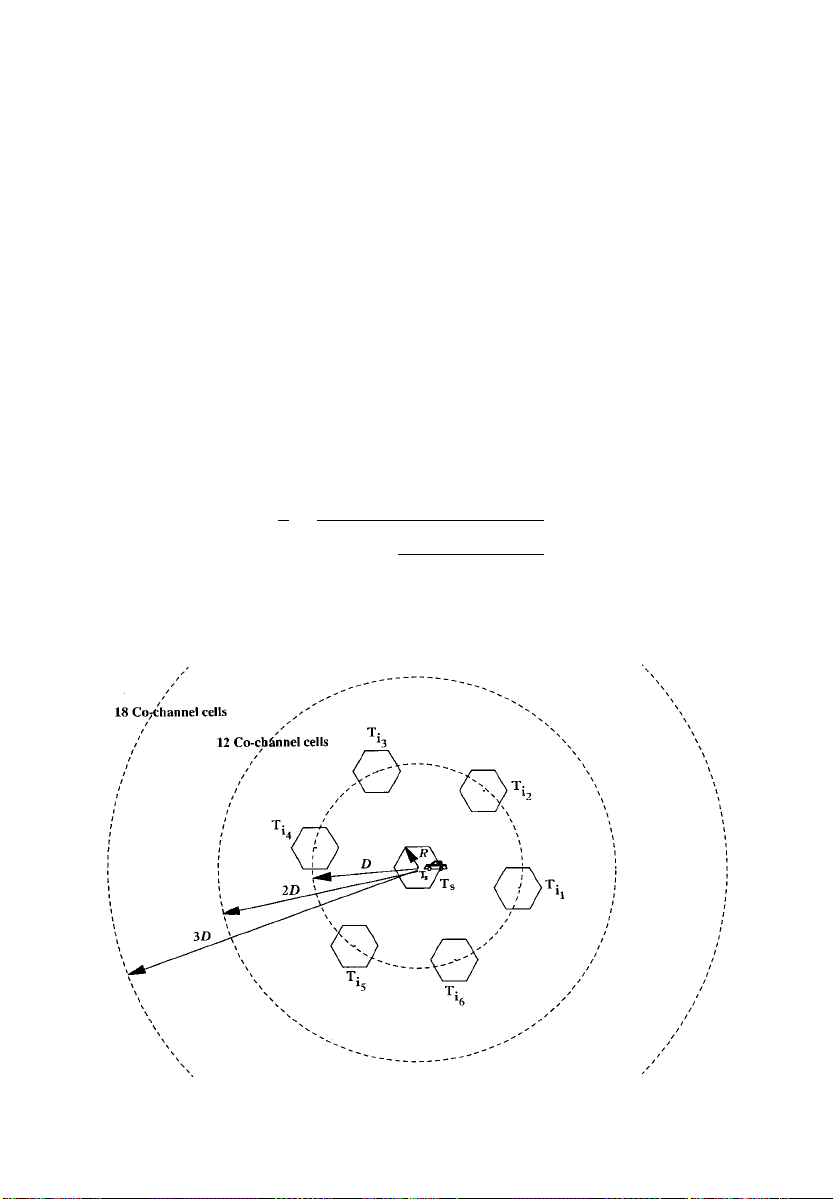
58

SPECTRAL EFFICIENCY OF ANALOGUE MODULATION TECHNIQUES

3.6.5 Model III: Geographical Model with Several Tiers of
Interferers

In this model, the co-channel interference from several tiers of co­channel cells is considered. In a fully equipped hexagon-shaped
cellular system, there are always 6m co-channel cells in the mth tier,
regardless of the number of cells per cluster. It is assumed that all co­channel interfering base stations, up to the mth tier considered, are
active as in a busy hour situation. It is also assumed that the
interference from cells in the higher order tiers (i.e. the m 1th tier
onwards) is negligible. This model is depicted in Figure 3.13, where R
and D have their usual meanings. For a hexagonal cellular system, the
average signal to interference ratio measured at a distance R from its
own serving station can be found in [3.21] and is given by the follow­ing relation:

=2

t1

3Nc

T

t1

X

u0

t

1

2

 u2 tu

: 3:88

=2

S



I

X

6

Hence, the following relations can be deduced:

Figure 3.13 Model III: Geographical Model with Several Tiers of Interferers

CO-CHANNEL INTERFERENCE MODELS 59





D

;

S



I

T

X

6

t1

()

 6



S

D
R

X

u0

I

t1

X

R

2

 u2 tu

t

T

t1

X

t1

u0

1

2

 u2 tu

t

=2

1

=2

3:89

1=

3:90

and

()

6

N



c



S

I

T

X

t1

t1

X

u0

2

 u2 tu

t

3

1

2=

=2

3:91

where T is the number of tiers of co-channel interfering cells consid­ered. Also, the normalized location of a unit cluster consisting of six
base stations at equal distances from the serving base station is
expressed by t; u. For example, the fourth tier can be expressed by
using four unit clusters:

t; u4; 0; 4; 1; 4; 2 and 4; 3:

Using Equation (3.90), the relationship between D=R and S=I can be
established for different numbers of tiers of interference. Similarly, the
relation between N

and S=I can be established for different numbers

c

of tiers of interference using Equation (3.91). The summation is evalu­ated for   4, without affecting the generality of the results.

(i) Considering only the first tier of interference with six co-channel
cells.

In this case, T  1 and t; u1; 0.

hi

D

R

 6

1=

S
I

3:92

and



1=

S

6

I

N



c

: 3:93

3

The above result agrees with the previous geographical model with
six interferers.

60 SPECTRAL EFFICIENCY OF ANALOGUE MODULATION TECHNIQUES

(ii) Considering two tiers of interference with a total of 18 co-channel
cells.

In this case, T  2 and t; u2; 0 and (2,1).

hi

D

 7:04

R

1=

S

I

3:94

and



2=

S

7:04

I

N



c

3

: 3:95

(iii) Considering three tiers of interference with a total of 36 co-channel
cells.

In this case, T  3 and t; u3; 0, (3,1) and (3,2).

hi

D

 7:36

R

1=

S

I

3:96

and

2=

S

7:36



I

N



c

: 3:97

3

(iv) Considering four tiers of interference with a total of 60 co-channel
cells.

In this case, T  4 and t; u4; 0, (4,1), (4,2) and (4,3).

hi

D

 7:50

R

1=

S

I

3:98

and

2=

S

7:50



N



c

I

: 3:99

3

(v) Considering five tiers of interference with a total of 90 co-channel
cells.

In this case, T  5 and t; u5; 0, (5,1), (5,2), (5,3) and (5,4).

hi

D

 7:57

R

1=

S

I

3:100

CO-CHANNEL INTERFERENCE MODELS 61

Figure 3.14 Model III: Geographical Model with Several Tiers of Interferers.
Protection Ratio Versus D/R and Nc.ÐÐ, Five Tiers of Interference;± ± ±, One
Tier of Interference

and

2=

S

7:54



I

N



c

: 3:101

3

When considering more than five tiers of interference, no significant
change in Equations (3.100) and (3.101) is achieved. In fact, the rela­tion D=R versus the protection ratio in Figure 3.14 shows no signific­ant difference between the case of one tier of interferers and the case

62 SPECTRAL EFFICIENCY OF ANALOGUE MODULATION TECHNIQUES

of five tiers of interferers. This is because, although higher order
interference tiers contain more co-channel interfering cells, they are
further away from the serving base station at multiples of D (see
Figure 3.13). The interfering signal power received at the mobile
station from any interfering cell is given by:





1

I

t

!

tD

3:102

where t is the order of the interfering tier in which the interfering cell
resides. Hence, the interfering signal power falls more rapidly with
distance by a factor of t



, compared with the interfering signal power

received from the first tier. To give an example, for   4, the inter­fering signal power of a co-channel cell in the first tier is 625 times the
interfering signal power of a co-channel cell in the fifth tier. That is to
say:

I



1

 t

I

t

I

1

 54 625 29dB: 3:104

I

5

3:103

Considering that there are 30 co-channel interfering cells in the
fifth tier compared with only six co-channel interfering cells in the
first tier, the total interference power contributed by the first tier is
about 21 dB higher than the total interference power contributed by
the fifth tier.

The relations D=R versus S=I in decibels, and N

versus S=I (S=I is

c

the protection ratio, a) are illustrated in Figure 3.14, for different
possible values of .

An alternative method to evaluate the interference from several
tiers of co-channel cells is developed in Appendix A, leading to
similar results to the above.

3.6.6 Model IV: Fading only Statistical Model

In this model, the received signals at the mobile station are assumed to
have an amplitude which is varying with a Rayleigh distribution (see
Figure 3.15(a) ). The fading of the wanted and interfering signals are
assumed to be uncorrelated and the shadowing effects on the signals
are ignored. This model is based on one interferer, where the mobile

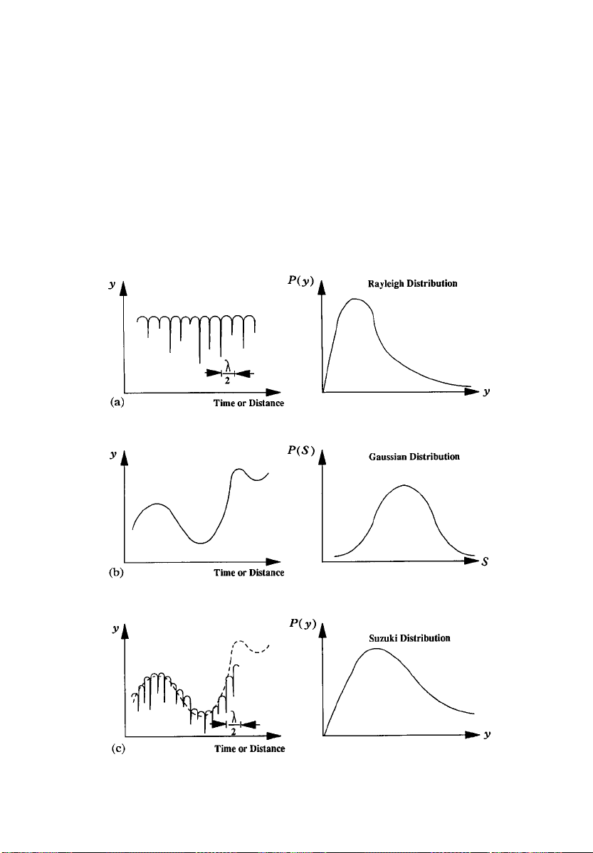
CO-CHANNEL INTERFERENCE MODELS 63

station is located between Tsand Tiat a distance xD from Ts, where
0 < x < 1. Suppose that the signal amplitude received at the mobile
station from the serving base station T
base station T

is yi, then for satisfactory reception it is necessary that :

i

 ry

y

s

is ysand from the interfering

s

i

where r is the `amplitude' protection ratio. We need to calculate the
probability of y

being greater than yiby the amount of the amplitude

s

protection ratio, r. For a variable y which is Rayleigh distributed with

Figure 3.15 (a) Model IV: Fading Only Statistical Model. (b) Model V: Shadow­ing Only Statistical Model. (c) Model VI: Fading and Shadowing Statistical Model

64 SPECTRAL EFFICIENCY OF ANALOGUE MODULATION TECHNIQUES

modal value , the probability density function (PDF) of the distribu­tion is:



exp

2

y

: 3:105

2

2

py



y

2



The probability P

To obtain the probability P
to integrate this function over all y



P

2





; P



2

that ys ryiat a given yiis:

1

Z

1

P

Z

0

Z

0

Z

0

r2

1

1

1



1

P1pyidy

exp



y

i
2



i

2



s

2

 

i

pysdys exp

ry

i

that ys> ryifor all yiit is only necessary

2

i



r2y

2

exp

: 3:109

2

s



2

i

2

s



y

2

, thus:

i

y

i
2



i

2

i



exp



2

r

2



s

2

r2y

i

: 3:106

2

2

s



2

y

i

dy

2

2

i







i

1

dy

2

i

3:107

3:108

i

The mean signal power is an inverse function of the distance between
the transmitter and the receiver (the inverse 

th

power law). Hence, at

the mobile station:

2



Ws1  xD

s



where W

2



i

2



s

;

2



i

and Wiare the omnidirectionally radiated powers from T

s

WixD

Ws1  x



Wix

and Tirespectively.

Substituting Equation (3.111) in (3.109), P



P

2

Ws1  x

r2Wix Ws1  x









becomes:

2



: 3:112



3:110

3:111

s

CO-CHANNEL INTERFERENCE MODELS 65

P2is the probability that the wanted signal ysis received at a level
above the interfering signal y

by the desired amplitude protection

i

ratio r. This result was developed by Gosling [3.15, 3.22] for   4 and
a similar result to Equation (3.109) was obtained in [3.21]. Following
the assumption that the co-channel interference is independent of the
actual amount of power transmitted by the base stations and that the
size of all cells are roughly the same, W

 Wi. Furthermore, consid-

s

ering the worst case of interference when the mobile station is nearest
to the interfering base station T
base station T

, xD  R and Equation (3.112) can be rewritten as

s

and furthest from its own serving

i

follows:





D



R

1  P

P

2

2



S

I

1=

1 3:113

and

()



N



P



c

2

1  P

2



S

I

1=

where S=I is the `power' protection ratio a, where a  r

1

2

3:114

2

. Equations
(3.113) and (3.114) are similar to Equations (3.78) and (3.79) obtained
using the geographical model with one interferer, except for the
protection ratio required by the fading only statistical model, which
is scaled by a factor of P

=1  P2. For 90% and 99% fading, the

2

required protection ratio of a particular modulation technique using
the fading only statistical model needs to be better by 9.5 dB and 20 dB
respectively, compared with the geographical model with one inter­ferer, to maintain the same spectral efficiency and voice quality. It can
be shown that Equations (3.113) and (3.114) become identical to Equa­tions (3.78) and (3.79) respectively for P
coincide for P

 50%).

2

The relations D=R versus S=I in decibels, and N

the protection ratio, a) are illustrated in Figure 3.16, for P

P

 99%,   4.

2

 50% (i.e. the two models

2

versus S=I (S=I is

c

 90% and

2

3.6.7 Model V: Shadowing only Statistical Model

In this model, the received signals (both wanted and interfering) at the
mobile station are assumed to suffer shadowing effects as a result of

66

SPECTRAL EFFICIENCY OF ANALOGUE MODULATION TECHNIQUES

Figure 3.16 Model IV: Fading Only Statistical Model. Protection Ratio Versus

D/R and N

. One Interferer, Worst Case,   4

c

the signal being blocked by large structures such as hills and moun­tains (Figure 3.15(b) ). The shadowing of the wanted and interfering
signals are assumed to be uncorrelated and the fading effects on the
signals are ignored. For shadowing, the variation in the received
signal level measured in decibels is best described by a normal
(Gaussian) distribution. The probability of 10 log y
than a
where a

 10 log y

dB

is the protection ratio in decibels. The relations D=R versus

dB

S=I in decibels, and N

2

 is developed and numerically evaluated in [3.7],

i

versus S=I are graphically presented in

c

2

 being greater

s

Figure 3.17 for 90% and 99% shadowing with standard deviations
  6 dB and 12 dB,   4.

CO-CHANNEL INTERFERENCE MODELS 67

Figure 3.17 Model V: Shadowing Only Statistical Model. Protection Ratio Ver­sus D/R and N
dB; B, 90% Shadowing,   12 dB; C, 99% Shadowing,   6 dB; D, 90% Shadow­ing,   6dB

. One Interferer. Worst Case,   4. A, 99% Shadowing,   12

c

3.6.8 Model VI: Fading and Shadowing Statistical Model

In land mobile radio, fading and shadowing of the received signal are
not separated from each other. The fading and shadowing statistical
model considers the general case when both the desired and interfer­ing signals are undergoing fading and shadowing effects simulta­neously, in an uncorrelated manner. In this case, the signal local
mean varies log-normally with a superimposed fading which follows
a Rayleigh distribution as shown in Figure 3.15(c). The superimposi-

68

SPECTRAL EFFICIENCY OF ANALOGUE MODULATION TECHNIQUES

Figure 3.18 Model VI: Fading and Shadowing Statistical Model. Protection Ratio
Versus D/R and N
Shadowing; B, 99% Fading + 6 dB Shadowing; C, 90% Fading + 12 dB Shadowing;
D, 90% Fading + 6 dB Shadowing

. One Interferer, Worst Case,   4. A, 99% Fading + 12 dB

c

tion of the two types of variations (i.e. Rayleigh and log±normal) is
sometimes referred to as the Suzuki distribution [3.20, 3.23]. Using
this distribution, the probability of the wanted signal y
than the interfering signal y

by the amount of the protection ratio is

i

being greater

s

developed and evaluated in [3.7]. Based on a one-interferer situation,
the relations D=R versus S=I in decibels, and N

versus S=I are

c

graphically presented in Figure 3.18 for 90% and 99% fading plus
shadowing with standard deviations   6 dB and 12 dB,   4.

COMPARISON OF THE VARIOUS MODELS 69

3.7 COMPARISON OF THE VARIOUS MODELS Comparisonofthe VariousModels

Figure 3.19 shows the re-use ratio D=R and the number of cells
per cluster N
co-channel interference models developed earlier. Knowing the pro­tection ratio of a modulation technique, the number of cells per cluster

N

required for a quality voice reception can be predicted using

c

Figure 3.19. Hence the modulation spectral efficiency is evaluated
using Equation (3.61). However, we need to compare the various co-

as a function of the protection ratio, for the six different

c

Figure 3.19 Comparison of Various Co-channel Interference Models.   4.ÐÐ,
(A) Geographical Model with Six Interferers;±.±.±, (B) Geographical Model with
90 Interferers;±..±..±, (C) Geographical Model with One Interferer;Ð Ð Ð Ð,

(D) Fading (90%) Only Statistical Model; . . . ...., (E) Shadowing Only Statistical

Model, 90% Shadowing,   6 dB;- - - - - - -, (F) Statistical Model, 90% Fading and
6 dB Shadowing

70 SPECTRAL EFFICIENCY OF ANALOGUE MODULATION TECHNIQUES

channel interference models in order that the best model can be used.
Comparing these models, the following points can be concluded:

(a) In general, the geographical models are easier to develop and use.

(b) The geographical model with six interferers provides a good
compromise between the two other geographical models. The
geographical model with one interferer is not a realistic situation,
whilst considering several tiers of interference achieves very little
benefit as shown in Figure 3.19. The geographical model with six
interferers is based on the assumption that all the interferers are active
all the time which is a somewhat extreme case for the following
reasons:

(i)ii not all the interferers are active all the time;

(ii)i on average, for half the time the interferer is transmitting and

for the other half it is receiving;

(iii) there is a time of silence between syllables, during which the

interference can be reduced if quieting techniques, such as
voice activated transmission, are employed in the mobile
system.

Regarding the first objection, the assumption that all six co-channel
interfering cells are active facilitates a busy hour situation. On the
other hand, the model is designed based on the worst case to show the
potential of a given modulation technique, although considering less
than six interferers is mathematically trivial by manipulating the
integer six in Equation (3.86). Furthermore, the practical considera­tions in (ii) and (iii) can be included in the conditions under which the
protection ratio is subjectively assessed.

(c) Although fading and shadowing effects are not considered when
the geographical models are developed, their effects on the signal can
be included in the value of the protection ratio. This is achieved by
performing subjective measurements to assess the value of the protec­tion ratio for various modulation techniques under fading and shad­owing conditions.

(d) Considering the statistical model category, the model with fad­ing and shadowing accounts for the general situation which charac­terizes the mobile radio channel. The shadowing only statistical
model is useful in urban areas with high rise buildings and in hilly

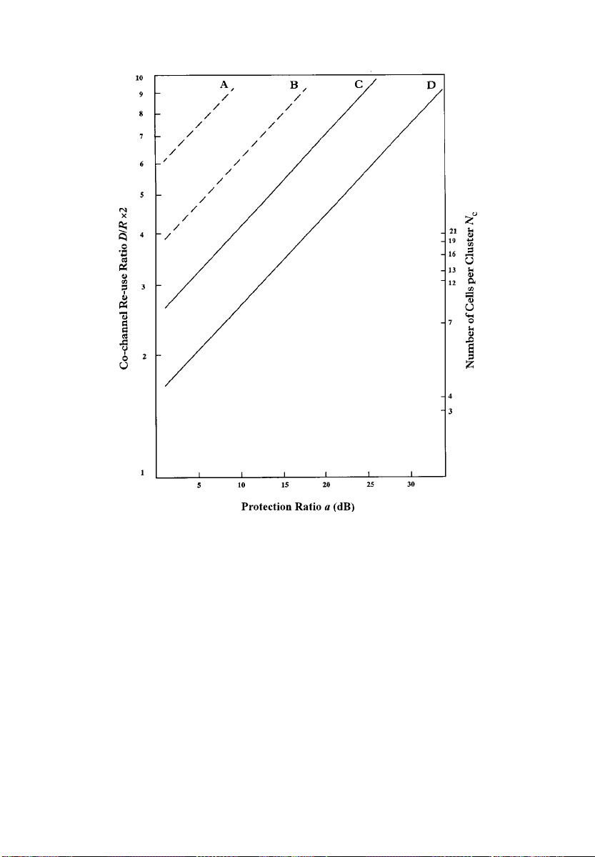
COMPARISON OF THE VARIOUS MODELS 71

Figure 3.20 Fading and Shadowing Statistical Models for One and Six Inter­ferers. Protection Ratio Versus D/R and N
Interferers. A, 90% Fading + 12 dB Shadowing; B, 90% Fading + 6 dB Shadowing;
C, 90% Fading + 12 dB Shadowing; D, 90% Fading + 6 dB Shadowing

:  4.ÐÐ, One Interferer;± ± ±, Six

c

areas. Also, mobile radio systems may adopt some means of diversity
reception which will greatly reduce fading, in which case the shadow­ing only model is suitable. The fading only statistical model is suitable
for suburban and low rise city locations. The fading only model is also
useful when line of sight reception is available, which is a rare case in
urban and suburban areas, especially with the low height antennas
used in cellular systems.

(e) The major drawbacks in the statistical models are their complex­ity and in the unrealistic assumption of one interferer only. Attempts
to account for all six interferers in the first tier of co-channel cells

72 SPECTRAL EFFICIENCY OF ANALOGUE MODULATION TECHNIQUES

[3.24] adds further complexity to the statistical models making them
more difficult to apply.

(f) Furthermore, the way in which the statistical models are used by
their advocates is ambiguous. If the protection ratio for a particular
modulation system is to be subjectively assessed under fading and
shadowing conditions and the statistical model with fading and
shadowing is used, then large values of re-use distances appear to
be necessary. For example, the protection ratio for 25/30 kHz FM
cellular land mobile radio systems is in the range of 17±18 dB [3.6];
according to the statistical model with 90% fading and 6 dB shadow­ing the number of cells per cluster required for quality voice reception
is 21, which does not comply with established cellular systems
such as AMPS and TACS, which use only seven cells per cluster.
Statistical models which account for all six closest interfering base
stations [3.24] exhibit drastically higher predicted values of re-use
distances D=R (and hence N

) as illustrated in Figure 3.20. On the

c

other hand, the statistical models inherently assume that fading and
shadowing cause identical deterioration to the signal regardless of the
modulation technique employed. This may be true for shadowing
since it is primarily a function of the topography near the mobile
station, however, fading may have different effects on the signal
according to the modulation technique employed. FM signal to
noise performance, for instance, can be severely affected by fading
near its threshold, unlike linear modulation techniques such as SSB
with the signal to noise performance deteriorating more gradually
with fading.

As a result, although the statistical models appear attractive to use,
they do not represent the practical situation. I feel strongly in favour
of the geographical model with six interferers. It is a useful tool in
assessing the spectral efficiency of cellular systems, provided that the
values of protection ratio used are subjectively evaluated for various
modulation systems under fading and shadowing conditions.

3.7.1 Mathematical Justification of the Geographical Models

Analytical results for propagation over a `plane earth' have been
derived by Norton and simplified by Bullington [3.17]. For base sta­tion and mobile station antenna elevated heights h

and hM, respect-

B

ively above ground level and separated a distance d apart, the

COMPARISON OF THE VARIOUS MODELS 73

received power PRis given in terms of the transmitted power PTas
follows:

2

GTG

4

d

R

3:115

where G

 P

hBhM

T

P

R

and GRare the gain of the transmitter antenna and receiver

T

antenna respectively. Based on the above equation and considering
the geographical model with one interferer, the desired signal power

S received at the mobile station from its own serving base station is:

R

2

GBsG

4

M

is the mobile station

M

3:116

hBshM

s

where W

S  W

is the power transmitted by the serving base station, hBsis

s

the serving base station antenna height, h
antenna height, G

is the serving base station antenna gain and G

Bs

is the mobile station antenna gain.

Similarly, the interfering signal power I received at the mobile

station from the interfering base station is:

D

2

GBiG

4

M

3:117

where W

I  W

is the power transmitted by the interfering base station, h

i

hBihM

i

is the interfering base station antenna height and GBiis the interfering
base station antenna gain.

Hence, combining the results in Equations (3.116) and (3.117) yields:

M

Bi

WsD4hBs2G

S



I

WiR4hBi2G

Bs

: 3:118

Bi

A similar relation can be derived for the geographical model with six
interferers.

From Equation (3.118), it can be seen that S/I can be maximized by

maximizing W

, hBsand GBs. However, this is not feasible from the

s

point of view of a mobile in the interfering co-cell, since that would
lead to minimizing its S=I. As a result, it can be trivially shown that
the optimum value for S=I within a cellular system is:



S
I

opt:





D
R

4

3:119

74 SPECTRAL EFFICIENCY OF ANALOGUE MODULATION TECHNIQUES

which agrees with our results before based on the assumption of equal
radiated power (i.e. equal cell sizes) and identical system parameters
within the cellular system. Nevertheless, Equation (3.119) remains
valid for mixed cell sizes when the cellular system is still growing.
Equation (3.119) also represents the general case when W

h

6 hBiand GBs6 GBi.

Bs

6 Wi,

s

3.8 SPECTRAL EFFICIENCY OF MODULATION

TECHNIQUES BASED ON THE SIX-INTERFERER
GEOGRAPHICAL MODEL

The efficiency of a modulation technique in a cellular system in terms
of Channels/MHz/km

2

is given by Equation (3.61) as: SpectralEfficiencyofModulation Techniques

1

M

B

cNc

A

:

The geographical model with six interferers establishes the relation­ship between the number of cells per cluster N
ratio of the modulation technique employed. In theory, N
take particular integer values (e.g. N
sequently suggests that N

is a discontinuous function of the protec-

c

 1, 3, 4, 7, 9, etc.), which con-

c

tion ratio. This restriction imposed on the values of N

and the protection

c

can only

c

stems from the

c

assumptions of a rigid hexagonal cell structure and each base station
being located exactly at the centre of its cell. In practice, however, such
a regular structure cannot be envisaged or imposed. Furthermore,
because of environmental, legal and zoning restrictions as well as site
availability problems it is not always possible to place the base station
at its grid point. In fact, current designs of cellular systems permit a cell
site to be positioned up to one-quarter of the nominal cell radius away
from the ideal location [3.6]. For these reasons, no restrictions are
imposed on the value of N

and, hence, using the six-interferer geo-

c

graphical model, the spectral efficiency of a modulation technique in a
cellular system is a function of the protection ratio. This is achieved by
substituting for N

from Equation (3.86), whence:

c





M

B

c

Equation (3.120) shows that 

M

parameters: the channel spacing B

3

: 3:120

2=

6a

A

is a function of four system

, protection ratio a, propagation

c

SPECTRAL EFFICIENCY OF MODULATION TECHNIQUES 75

constant  and the cell area A. The channel spacing and the protection
ratio are directly related to the modulation technique, and since the
protection ratio is representative of the voice quality, it needs to be
subjectively assessed under realistic conditions. The propagation con­stant  is dependent upon the nature of the terrain and urbanization

Figure 3.21 Probability of Message Completion. Mobile Speed in km/h is Indi­cated on the Curves. (a) Three-Minute Message. (b) One-Minute Message

76 SPECTRAL EFFICIENCY OF ANALOGUE MODULATION TECHNIQUES

degree and usually has values between three and four which can be
verified by means of field measurements. The cell area is governed by
several factors which are now discussed.

3.8.1 Factors Governing the Cell Area A

Equation (3.120) shows that the spectral efficiency of a modulation
technique in a cellular system is inversely proportional to the cell area.
Hence, the spectral efficiency can be maximized by minimizing the
cell area. Theoretically, cellular systems can continue to grow indefin­itely through the process of cell splitting. Nevertheless, there are
several factors which will limit the minimum cell area which can be
achieved in practice.

(a) For small cells, the hand-off rate becomes unacceptably high.
Figure 3.21 shows the probability of completion of messages of three
minutes and one minute duration as a function of the cell radius
[3.25]; the probability of hand-off is deduced.

(b) Paging mobiles within the cellular system becomes more difficult
to handle for smaller cells.

(c) Co-channel interference becomes more difficult to manage for
smaller cell sizes, especially considering the co-existence of other
radio systems. In addition, errors in the location, hand-off and
power control processes make reliable interference control more diffi­cult as cells become smaller.

(d) As cells become smaller and smaller, more control channels are
required for the purpose of call set-up, monitoring, supervision, hand­off, etc. This in turn will reduce the spectral efficiency since more
channels are dedicated for control functions rather than being used
for voice communication.

(e) Environmental, legal and zoning restrictions as well as site avail­ability problems become more difficult as cells become smaller.

The above considerations are the dominant factors in restricting the
minimum cell radius which can be employed in practice. Cells as
small as 1.5 km in radius appear to be practical [3.25]. In our opinion,
a cell radius as small as 1 km A  3km

2

 is possible with the present

technologies. This value will be used in the efficiency comparisons of
various cellular systems.

REFERENCES 77

REFERENCES REFERENCES

[3.1] Brewster, R. L., 1986 Telecommunication Technology, Ellis Horwood

Series in Electronics and Communication Engineering John Wiley and

Sons, Chichester

[3.2] Shanmugam, K. S., 1979 Digital and Analog Communication Systems

John Wiley and Sons, New York

[3.3] Schwartz, M., 1970 Information Transmission, Modulation, and Noise,

Second Edition, McGraw-Hill Kogakusha, Tokyo

[3.4] Stremler, F. G., 1982 Introduction to Communication Systems, Addison-

Wesley Series in Electrical Engineering Second Edition Publishing Com­pany, Reading, MA

[3.5] Lee, W. C. Y., 1986 Elements of Cellular Mobile Radio Systems, IEEE

Trans. Veh. Technol. VT-35 (2) May pp. 48±56

[3.6] MacDonald, V. H., 1979 Advanced Mobile Phone Services: The cellular

Concept Bell Sys. Tech. J. 58 (1) January pp. 15±43

[3.7] French, R. C., 1979 The Effect of Fading and Shadowing on Channel

Re-use in Mobile Radio IEEE Trans. Veh. Technol. VT-28, (3) August pp.
171±81

[3.8] CCIR, 1986 Report 358±5, XVI Plenary Assembly, Dubrovnik, Vol. VIII-

1, International Telecommunication Union pp. 3±13

[3.9] Bullington, K., 1984 Radio Propagation for Vehicular Communication

Land Mobile Communication Engineering IEEE Press, New York (Rep­rinted from: 1977 IEEE Trans. Veh. Technol. VT-26, November pp. 295±

308)

[3.10] Okumura, Y., et al., Field Strength and its Variability in VHF and

UHF Land-Mobile Radio Service Land Mobile Communication Engineering
IEEE Press, New York . (Reprinted with permission from: 1968 Rev. Elec.
Commun. Lab., 16, September±October pp. 825±73).

[3.11] Young, W. R., Jnr, 1986 Comparison of Mobile-Radio Transmission at

150, 450, 900 and 3700 Mc Land Mobile Communication Engineering IEEE
Press, New York (Reprinted from: 1952 Bell Syst. Tech. J. 31, November
pp. 1068±85)

[3.12] Black, D. M., 1984 Some Characteristics of Mobile-Radio Propagation

at 836 MHz in the Philadelphia Area Land Mobile Communication Engi-

neering, IEEE Press, New York (Reprinted from: 1972 IEEE Trans. Veh.
Technol VT-21, May pp. 45±51)

[3.13] IEEE Vehicular Technology Society Committee on Radio Propaga-

tion. Coverage Prediction for Mobile Radio Systems Operating in the
800/900 MHz Frequency Range. 1988 IEEE Trans. on Veh. Technol. Special
Issue on Mobile Radio Propagation VT-37, (1) February

[3.14] Hata, M., Kinoshita, K. and Hirade, K., 1984 Radio Link Design of

Cellular Land Mobile Communication Systems Land Mobile Communica-

tion Engineering IEEE Press, New York (Reprinted from: 1982 IEEE Trans.
Veh. Technol. VT-31, February pp. 25±31)

78 SPECTRAL EFFICIENCY OF ANALOGUE MODULATION TECHNIQUES

[3.15] Gosling, W., 1978 A Simple Mathematical Model of Co-channel and

Adjacent Channel Interference in Land Mobile Radio Radio and Electron.
Eng. 48 (12) December pp. 619±22

[3.16] Lee, W. C. Y., 1982 Mobile Communications Engineering, McGraw-

Hill, New York

[3.17] Reudink, D. O., 1984 Properties of Mobile Radio Propagation Above

400 MHz, Land Mobile Communication Engineering IEEE Press, New York
(Reprinted from: 1974 IEEE Trans. Veh. Technol. VT-23, November pp.
143±59)

[3.18] Nylund, H. W., 1984 Characteristics of Small Area Signal Fading on

Mobile Circuits in the 150 MHz Band Land Mobile Communication

Engineering IEEE Press, New York (Reprinted from: 1968 IEEE Trans.
Veh. Technol. VT-17, October pp. 24±30)

[3.19] Arredondo, G. A., Feggeler, J. C. and Smith, J. I., 1979 Advanced Mobile

Services: Voice and Data Transmission Bell Sys. Tech. J. 58 (1) January pp.
97±122

[3.20] Parsons, J. D., 1984 Propagation and Interference in Cellular Radio

Systems IEE Conference Publication Number 238, May 1984, pp. 71±5

[3.21] Daikoku, K. and Ohdate, H., 1983 Optimal Channel Re-use in Cellular

Land Mobile Radio Systems IEEE Trans. Veh. Technol., VT-32 (3) August
pp. 217±24

[3.22] Gosling, W., 1980 Protection Ratio and Economy of Spectrum Use in

Land Mobile Radio IEE Proc. 127 Pt F (3) June pp. 174±78

[3.23] Parsons, J. D. and Ibrahim, M. F., 1983 Signal Strength Prediction in

Built-up Areas; Part 2: Signal Variability IEE proc. 130, Pt F (5) August pp.
385±91

[3.24] Muammar, R. and Gupta, S. C., 1982 Co-channel Interference in High

Capacity Mobile Radio Systems IEEE Trans. Commun. COM-30 (8)
August pp. 1973±78

[3.25] CCIR, 1982 Report 740±1, XV Plenary Assembly, Geneva Vol. VIII,

International Telecommunication Union

4

Spectral Efficiency of Digital
Modulation Techniques

4.1 INTRODUCTION Introduction

Analogue modulation systems are well established for the transmis­sion of voice in today's cellular systems. Digital modulation systems,
however, are becoming increasingly popular for a variety of reasons.
First of all, digital modulation systems offer a very wide range of
possibilities, which in turn provide a great deal of flexibility. Digital
techniques incorporate enhanced capabilities more easily and allow
the integration of the components using VLSI (very large scale integra­tion) techniques, which result in smaller and, hopefully, cheaper
equipment. Also, digital cellular systems can easily be made compat­ible with the Integrated System Digital Network (ISDN) which can
support data as well as voice transmission. Furthermore, the use of
digital systems enables security through encryption to be easily
achieved ± an important requirement in today's world radio environ­ment. For such reasons, it is not so surprising that all nine systems
which were proposed for the Pan-European cellular mobile radio
system in the mid-eighties were digital [4.1] and that North America
and Japan were well advanced in their plans to implement digital
cellular systems. On the other hand, digital transmission is normally
greedy in its use of bandwidth [4.2] and since spectral efficiency is of
prime importance in the land mobile radio environment, the current
trend to assume that `digital is good and analogue is bad/old
fashioned' may not be justifiable.

In the previous chapter, the spectral efficiency of analogue modula­tion techniques within cellular land mobile radio system was evalu­ated. Although the method was mainly designed for analogue

SpectralEfficiencyof DigitalModulation Techniques

79

80 SPECTRAL EFFICIENCY OF DIGITAL MODULATION TECHNIQUES

modulation techniques, it can be easily applied to digital modulation
techniques. This is mainly because the interference models used are
independent of the modulation technique employed. Also, because of
the nature of digital systems and the way some parameters are
defined, voice channel spacing and the protection ratio need to be
evaluated so they can be used with the modulation efficiency equation
developed in Chapter 3. The channel spacing is usually defined in
terms of kbps and we need to evaluate that in kHz. Also, there is a
possibility of an objective assessment of the protection ratio using the
bit error rate (BER) as a quality measure.

In this chapter, two approaches to evaluate the channel spacing and
the protection ratio are presented. Consequently, a brief review of
digital modulation techniques is given and the key parameters
required for the evaluation are highlighted. The channel spacings of
digital modulation techniques are very much dependent on the voice
coding method used. It is necessary, therefore, to present a short
survey of the voice coding techniques available today. The channel
spacing of a digital modulation technique is then evaluated using a
theoretical as well as a practical method. The two approaches are
compared. It must be noted here that the objective of the exercise is
not to evaluate the channel spacing and the protection ratio for all
digital modulation techniques, but rather to show a systematic method
to evaluate them given the necessary parameters. The results are then
used in the modulation efficiency formula, developed in the previous
chapter. The spectral efficiency assessment of various analogue and
digital cellular land mobile radio systems is the subject of Chapter 6.

4.2 BASIC DIGITAL MODULATION TECHNIQUES BasicDigital ModulationTechniques

In digital modulation techniques, to convey information, a parameter
of a continuous high-frequency carrier is varied in proportion to a
low-frequency baseband digital message signal. The carrier to be
modulated has the following general form:

tvt cos wct  t wc 2 f

x

c

c

where v(t) is the instantaneous amplitude of the carrier, f
carrier frequency and t is the instantaneous phase deviation of
the carrier.

In general, there are three basic digital modulation techniques:
amplitude modulation (AM), frequency modulation (FM) and phase

is the

c

4:1

BASIC DIGITAL MODULATION TECHNIQUES 81

Figure 4.1 Primary Components of a Digital Radio Communication System

modulation (PM). In amplitude modulation, v(t) is linearly related to
the digital message signal m(t), in which case it is a linear process.
However, if t or its time derivative is linearly related to m(t), then
we have PM or FM respectively; these are non-linear processes. On
the other hand, each of the basic digital modulation techniques has a
large number of variants. Hybrid digital techniques are also possible
and have received increased attention in the recent years because of
their inherent economical use of spectrum [4.3].

A simple radio frequency digital communication system is shown in
Figure 4.1. The baseband digital message may be filtered, shaped, etc.
prior to modulating the carrier so that desirable results are achieved.
At the receiver, the baseband digital message is recovered using a
detection process. Basically, there are two types of detection: coherent
detection and non-coherent detection. In coherent detection, there is a
requirement for a sinusoidal carrier which is perfectly matched to
both the frequency and phase of the received carrier. Such a phase
reference may be obtained either from a transmitted pilot tone or from
the modulated signal itself. Non-coherent detection, however, is based
upon waveform characteristics independent of phase, such as amplit­ude or frequency, and hence does not require a phase reference.
Detection is usually followed by a decision process which converts
the recovered baseband digital message signal into a sequence of
digital bits. The decision process requires bit synchronization which
can be extracted from the received waveform.

82

SPECTRAL EFFICIENCY OF DIGITAL MODULATION TECHNIQUES

4.2.1 Digital Amplitude Modulation (AM) Techniques

The simplest digital amplitude modulation technique can be mathem­atically represented as follows:

xt

1  mt cos w

2

t4:2

c

1

where m(t) is a binary digital message signal. For the case of
mt1, then we have amplitude shift keying (ASK) or on±off key-
ing (OOK) modulation, this is depicted in Figure 4.2(b). ASK wave­form can be detected either coherently or non-coherently. However,
there is a slight difference in performance, compared to the increase in
complexity needed to maintain phase coherence between the trans­mitted signal and the local carrier.

Figure 4.2 Basic Digital Modulation Techniques. (a) Binary Modulating Signal.
(b) ASK Signal. (c) FSK Signal. (d) PSK Signal

BASIC DIGITAL MODULATION TECHNIQUES 83

The carrier in Equation (4.2) conveys no information, and hence
power efficiency can be improved by the use of a double-sideband
suppressed carrier (DSB-SC), which has the following general form:

xtmt cos w

t mt0or1: 4:3

c

Spectral efficiency can be improved by a factor of two by the use of
single-sideband (SSB) digital modulation with non-trivial practical
implementation and a considerable increase in complexity.

Another variation of AM is quadrature amplitude modulation
(QAM), which is obtained by summing two DSB-SC signals at 908
apart in phase. A quadrature amplitude modulated signal has the
following general form:

where m

xtm

t and mQt are independent binary data signals, in which

I

t cos wctmQt sin wct4:4

I

case QAM is as efficient in both required power and bandwidth as an
ideal SSB. Quadrature partial response (QPR) is obtained if m

m

t are three-level duobinary signals (1, 1 or 0) coded to affect

Q

t and

I

minimum intersymbol interference. Coherent detection is required for
QAM and QPR and hence any phase errors that occur result in inter­ference between the I and Q channels which in turn will degrade their
performance.

4.2.2 Digital Frequency Modulation (FM) Techniques

Frequency shift keying (FSK) is the simplest form of a digital FM
technique. FSK is generated by switching the frequency of the carrier
between two values ( f
signal; f

being small compared with the carrier frequency fc(see

1±f2

and f2), corresponding to a binary message

1

Figure 4.2(c)). It is a common practice in FSK modulation schemes to
specify the frequency spacing in terms of the modulation index, h,
which is defined as:

 f2T

1

b

b

4:5

where T

h f

h   fT

is the symbol duration.

b

FSK can be detected either coherently or non-coherently. Non­coherent detection of FSK can be achieved using two bandpass filters,
followed by envelope detectors and a decision circuit. It is also

84 SPECTRAL EFFICIENCY OF DIGITAL MODULATION TECHNIQUES

possible to detect FSK signals non-coherently, using a discriminator
followed by amplitude detection.

Other modified forms of FSK technique are also used. For example,
continuous phase FSK (CP-FSK) is used to avoid the abrupt phase
changes at bit transition instants and hence leading to improved
spectral efficiency. Optimal coherent detection of CP-FSK is achieved
with values of h in the vicinity of 0.7. Minimum shift keying (MSK) is a
special case of CP-FSK for which coherent detection with h  0:5is
used. Other forms of CP-FSK can be found in the literature [4.4].

4.2.3 Digital Phase Modulation (PM) Techniques

A well known basic type of phase modulation is binary phase shift
keying (BPSK), in which the carrier phase is shifted between two
values, 08 and 1808, as shown in Figure 4.2(d). BPSK modulation
requires coherent detection, in which case a precise phase reference
in the receiver is necessary. Differentially encoded PSK (DE-PSK) and
differential PSK (DPSK) are other modified versions of PSK. With DE­PSK, the binary digital message is conveyed via transitions in the
carrier phase. That is to say, no transition in phase corresponds to,
say, binary `0' and a 1808 transition corresponds to binary `1'. With
DPSK, the information is also differentially encoded, but a detector is
employed which uses the signal from the previous bit interval as a
phase reference for the current bit interval. The performance of both
DE-PSK and DPSK is somewhat inferior to that of coherent PSK.

4.2.4 M-Ary Digital Modulation Schemes

M-ary digital modulation schemes are just an extension to the basic
digital modulation techniques discussed earlier. In M-ary schemes, one
of M signals is transmitted during each signalling interval, where M is
greater than 2. Thus, we can have M-ary ASK such as 4-ASK and
16-QAM. QPSK, 8-PSK and 16-PSK are examples of M-ary PSK. With
M-ary FSK, one of a set of M possible carriers (or carrier frequencies) is
selected according to the modulating digital message. Figure 4.3 shows
constellation diagrams for some M-ary digital modulation schemes.

M-ary digital modulation schemes are often used whenever band­width needs to be conserved at the expense of power or vice versa; an
advantage which cannot be achieved with binary modulation tech­niques. M-ary PSK schemes are used to conserve bandwidth at the
expense of increased power requirements, while wideband M-ary

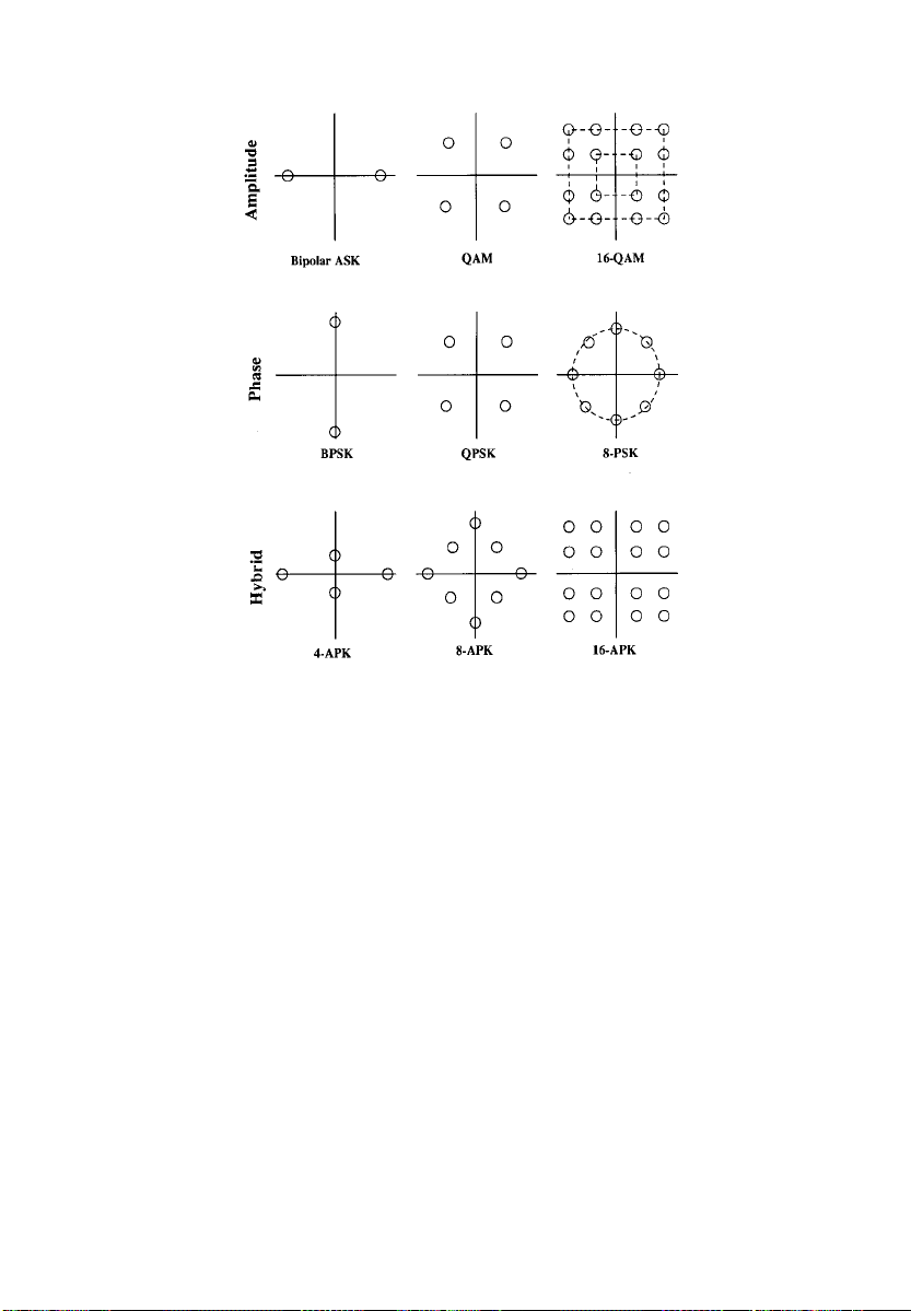
BASIC DIGITAL MODULATION TECHNIQUES 85

Figure 4.3 Constellation Diagrams for some M-ary Digital Modulation Schemes

FSK schemes utilize more bandwidth to provide increased immunity
to noise and conserve power.

4.2.5 Hybrid Digital Modulation Schemes

By combining two different digital modulation techniques, it is pos­sible to arrive at a hybrid scheme which out performs either technique
alone. The most commonly used hybrid technique is amplitude and
phase shift keying (APK). The main advantage of the APK scheme is
its superior bandwidth efficiency. An M-ary form of APK is usually
used for this reason and one example is 16-APK.

4.2.6 Performance Comparison of Various Digital Modulation
Techniques

The performance of digital modulation techniques can be compared
in a number of ways. However, we shall limit the comparison to those

86 SPECTRAL EFFICIENCY OF DIGITAL MODULATION TECHNIQUES

Table 4.1 Performance of Representative Set of Digital Modulation Techniques

Digital Modulation
and Detection

AM ASK-Envelope 1 < 0:8 11.9 19

ASK-C 1 0.8 11.4 17
QAM 2 1.7 8.4 14
QPR 2.5 2.25 10.7 16.5
16-QAM 4 3.0 14.4 21.5

FM FAK h  1NC 1 0.8 12.5 20

CP-FSK h  0:7NC 1 1.0 9.2 18
CP-FSK h  0:7C 1 1.0 7.4 13
MSK h  0:5C 2 1.9 8.4 14
MSK h  0:5DE 2 1.9 9.4 17

PM BPSK-C 1 0.8 8.4 14

DE-BPSK 1 0.8 8.9 17
DPSK 1 0.8 9.3 17
DQPSK 2 1.8 10.7 20
QPSK 2 1.9 8.4 13.5
8-PSK 3 2.6 11.8 16.5
16-PSK 4 2.9 16.2 21

AM/PM 4-APK 2 < 2 8.4 13.5

8-APK 3 2.8 9.4 15
16-APK 4 3.3 12.4 18

C, Coherent; NC, Non-coherent; DE, Differential Encoding. Data taken from a variety of
sources QAM/APK belong to the same family and should in theory have the same
performance.

Speed (bps/Hz) Eb=NodB

Theoretical Practical

Ideal
BER  10

4

Fading
BER  10

2

parameters which are particularly relevant to the assessment of spec­tral efficiency of various digital modulation techniques as applied to
cellular systems. The most important parameters governing the spec­tral efficiency of a digital modulation technique are the bandwidth
efficiency and the signal to noise performance required to achieve a
given bit error rate (BER).

The bandwidth efficiency of a digital modulation technique can be
conveniently characterized in terms of the transmitted bits per second
per Hertz (bps/Hz). This is also referred to as the `speed' of a mod­ulation technique and is now a standard term used in CCIR recom­mendations and regulations. In practice, implementation limitations
reduce the theoretical speed of various digital modulation techniques.
Table 4.1 shows some tabulated values of the theoretical and practical
speed of various modulation techniques taken from a number of
sources [4.3, 4.5, 4.6].

It is also important to compare different digital modulation tech­niques in terms of the signal to noise ratio (SNR) required to achieve a

BASIC DIGITAL MODULATION TECHNIQUES 87

Figure 4.4 BER Versus SNR for Some Digital Modulation Techniques. A, Coher­ent PSK; B, DPSK; C, Coherent FSK; D, Coherent ASK; E, Non-coherent FSK; F,
Non-coherent ASK

specific BER. The ideal BER performance of digital modulation tech­niques as a function of SNR in the presence of additive white Gaus­sian noise (AWGN) has been derived and well documented in many
sources (see for example [4.7]). The BER versus SNR for some digital
modulation techniques is plotted in Figure 4.4. Often, the BER perfor­mance is measured in terms of the average signal energy per bit to