WILEY Broadband Optical Access Networks User Manual

BROADBAND OPTICAL
ACCESS NETWORKS

BROADBAND OPTICAL
ACCESS NETWORKS

LEONID G. KAZOVSKY
NING CHENG
WEI-TAO SHAW
DAVID GUTIERREZ
SHING-WA WONG

A JOHN WILEY & SONS, INC., PUBLICATION



Copyright

C

2011 by John Wiley & Sons, Inc. All rights reserved.

Published by John Wiley & Sons, Inc., Hoboken, New Jersey.
Published simultaneously in Canada.

No part of this publication may be reproduced, stored in a retrieval system, or transmitted in any form or
by any means, electronic, mechanical, photocopying, recording, scanning, or otherwise, except as
permitted under Sections 107 or 108 of the 1976 United States Copyright Act, without either the prior
written permission of the Publisher, or authorization through payment of the appropriate per-copy fee to
the Copyright Clearance Center, Inc., 222 Rosewood Drive, Danvers, MA 01923, [phone],
fax [phone], or on the web at www.copyright.com. Requests to the Publisher for permission
should be addressed to the Permissions Department, John Wiley & Sons, Inc., 111 River Street, Hoboken,
NJ 07030, [phone], fax [phone], or online at http://www.wiley.com/go/permission.

Limit of Liability/Disclaimer of Warranty: While the publisher and author have used their best efforts in
preparing this book, they make no representations or warranties with respect to the accuracy or
completeness of the contents of this book and specifically disclaim any implied warranties of
merchantability or fitness for a particular purpose. No warranty may be created or extended by sales
representatives or written sales materials. The advice and strategies contained herein may not be suitable
for your situation. You should consult with a professional where appropriate. Neither the publisher nor
author shall be liable for any loss of profit or any other commercial damages, including but not limited to
special, incidental, consequential, or other damages.

For general information on our other products and services or for technical support, please contact our
Customer Care Department within the United States at [phone], outside the United States at
[phone] or fax [phone].

Wiley also publishes its books in a variety of electronic formats. Some content that appears in print may
not be available in electronic format. For more information about Wiley products, visit our web site at

www.wiley.com

Library of Congress Cataloging-in-Publication Data Is Available

Kazovsky, Leonid G.

Broadband optical access networks / Leonid G. Kazovsky, Ning Cheng, Wei-Tao Shaw, David

Gutierrez, Shing-Wa Wong.

Includes index.

ISBN 978-0-470-18235-2

Printed in Singapore

oBook ISBN: 978 0470 910931
ePDF ISBN: 978 0470 910924
ePub ISBN: 978 0470 922675

10987654321

CONTENTS

FOREWORD xi
PREFACE xiii
ACKNOWLEDGMENTS xv

1 BROADBAND ACCESS TECHNOLOGIES: AN OVERVIEW 1

1.1 Communication Networks / 2

1.2 Access Technologies / 4

1.2.1 Last-Mile Bottleneck / 4

1.2.2 Access Technologies Compared / 5

1.3 Digital Subscriber Line / 6

1.3.1 DSL Standards / 7

1.3.2 Modulation Methods / 8

1.3.3 Voice over DSL / 8

1.4 Hybrid Fiber Coax / 9

1.4.1 Cable Modem / 10

1.4.2 DOCSIS / 10

1.5 Optical Access Networks / 11

1.5.1 Passive Optical Networks / 11

1.5.2 PON Standard Development / 12

1.5.3 WDM PONs / 13

1.5.4 Other Types of Optical Access Networks / 15

v

vi CONTENTS

1.6 Broadband over Power Lines / 18

1.6.1 Power-Line Communications / 18

1.6.2 BPL Modem / 19

1.6.3 Challenges in BPL / 20

1.7 Wireless Access Technologies / 20

1.7.1 Wi-Fi Mesh Networks / 21

1.7.2 WiMAX Access Networks / 22

1.7.3 Cellular Networks / 24

1.7.4 Satellite Systems / 25

1.7.5 LMDS and MMDS Systems / 26

1.8 Broadband Services and Emerging Technologies / 28

1.8.1 Broadband Access Services / 29

1.8.2 Emerging Technologies / 30

1.9 Summary / 31
References / 33

2 OPTICAL COMMUNICATIONS: COMPONENTS

AND SYSTEMS 34

2.1 Optical Fibers / 35

2.1.1 Fiber Structure / 35

2.1.2 Fiber Mode / 38

2.1.3 Fiber Loss / 45

2.1.4 Fiber Dispersion / 47

2.1.5 Nonlinear Effects / 52

2.1.6 Light-Wave Propagation in Optical Fibers / 54

2.2 Optical Transmitters / 55

2.2.1 Semiconductor Lasers / 55

2.2.2 Optical Modulators / 66

2.2.3 Transmitter Design / 71

2.3 Optical Receivers / 72

2.3.1 Photodetectors / 73

2.3.2 Optical Receiver Design / 76

2.4 Optical Amplifiers / 78

2.4.1 Rare-Earth-Doped Fiber Amplifiers / 81

2.4.2 Semiconductor Optical Amplifiers / 83

2.4.3 Raman Amplifiers / 85

2.5 Passive Optical Components / 86

2.5.1 Directional Couplers / 86

2.5.2 Optical Filters / 89

CONTENTS vii

2.6 System Design and Analysis / 93

2.6.1 Receiver Sensitivity / 93

2.6.2 Power Budget / 98

2.6.3 Dispersion Limit / 99

2.7 Optical Transceiver Design for TDM PONs / 101

2.7.1 Burst-Mode Optical Transmission / 102

2.7.2 Colorless ONUs / 104

2.8 Summary / 106
References / 107

3 PASSIVE OPTICAL NETWORKS: ARCHITECTURES

AND PROTOCOLS 108

3.1 PON Architectures / 109

3.1.1 Network Dimensioning and Bandwidth / 110

3.1.2 Power Budget / 110

3.1.3 Burst-Mode Operation / 112

3.1.4 PON Packet Format and Encapsulation / 113

3.1.5 Dynamic Bandwidth Allocation, Ranging,

and Discovery / 114

3.1.6 Reliability and Security Concerns / 114

3.2 PON Standards History and Deployment / 115

3.2.1 Brief Developmental History / 115

3.2.2 FTTx Deployments / 116

3.3 Broadband PON / 117

3.3.1 BPON Architecture / 118

3.3.2 BPON Protocol and Service / 121

3.3.3 BPON Transmission Convergence Layer / 125

3.3.4 BPON Dynamic Bandwidth Allocation / 130

3.3.5 Other ITU-T G.983.x Recommendations / 133

3.4 Gigabit-Capable PON / 133

3.4.1 GPON Physical Medium–Dependent Layer / 134

3.4.2 GPON Transmission Convergence Layer / 137

3.4.3 Recent G.984 Series Standards, Revisions, and

Amendments / 142

3.5 Ethernet PON / 144

3.5.1 EPON Architecture / 144

3.5.2 EPON Point-to-Multipoint MAC Control / 147

3.5.3 Open Implementations in EPON / 152

3.5.4 Unresolved Security Weaknesses / 155

viii CONTENTS

3.6 IEEE 802.av-2009 10GEPON Standard / 156

3.6.1 10GEPON PMD Architecture / 156

3.6.2 10GEPON MAC Modifications / 158

3.6.3 10GEPON Coexistence Options / 161

3.7 Next-Generation Optical Access System Development
in the Standards / 162

3.7.1 FSAN NGA Road Map / 162

3.7.2 Energy Efficiency / 163

3.7.3 Other Worldwide Development / 164

3.8 Summary / 164
References / 165

4 NEXT-GENERATION BROADBAND OPTICAL

ACCESS NETWORKS 166

4.1 TDM-PON Evolution / 167

4.1.1 EPON Bandwidth Enhancements / 168

4.1.2 GPON Bandwidth Enhancements / 168

4.1.3 Line Rate Enhancements Research / 169

4.2 WDM-PON Components and Network Architectures / 172

4.2.1 Colorless ONUs / 173

4.2.2 Tunable Lasers and Receivers / 174

4.2.3 Spectrum-Sliced Broadband Light Sources / 176

4.2.4 Injection-Locked FP Lasers / 178

4.2.5 Centralized Light Sources with RSOAs / 179

4.2.6 Multimode Fiber / 181

4.3 Hybrid TDM/WDM-PON / 184

4.3.1 TDM-PON to WDM-PON Evolution / 184

4.3.2 Hybrid Tree Topology Evolution / 186

4.3.3 Tree to Ring Topology Evolution / 195

4.4 WDM-PON Protocols and Scheduling Algorithms / 202

4.4.1 MAC Protocols / 203

4.4.2 Scheduling Algorithms / 204

4.5 Summary / 211
References / 211

5 HYBRID OPTICAL WIRELESS ACCESS NETWORKS 216

5.1 Wireless Access Technologies / 217

5.1.1 IEEE 802.16 WiMAX / 217

5.1.2 Wireless Mesh Networks / 225

CONTENTS ix

5.2 Hybrid Optical–Wireless Access Network Architecture / 241

5.2.1 Leveraging TDM-PON for Smooth Upgrade of Hierarchical
Wireless Access Networks / 242

5.2.2 Upgrading Path / 244

5.2.3 Reconfigurable Optical Backhaul Architecture / 247

5.3 Integrated Routing Algorithm for Hybrid Access Networks / 258

5.3.1 Simulation Results and Performance Analysis / 260

5.4 Summary / 262
References / 263

INDEX 267

FOREWORD

Broadband optical access networks are crucial to the future development of the
Internet. The continuing evolution of high-capacity, low-latency optical access net­works will provide users with real-time high-bandwidth access to the Web essential
for such emerging trends as immersive video communications and ubiquitous cloud
computing. These ultrahigh-speed access networks must be built under challenging
economic and environmental imperatives to be “faster, cheaper, and greener.” T his
book presents in a clear and illustrative format the technical and scientific concepts
that are needed to accomplish the design of new broadband access networks upon
which users will surf the wave of the twenty-first-century Internet.

The book is coauthored by Professor Leonid Kazovsky and his graduate stu­dents. Professor Kazovsky is a recognized leader and authority in the field and has
a long and distinguished track record for making highly timely and significant re­search contributions within the general area of optical communication systems and
optical networks.He has contributed over thelast 40 years in the areas of wavelength­division-multiplexed(WDM) andcoherent transmission systems for the core network
as well as transmission systems and network architectures and technologies at the
metro and access levels. This book builds on Professor Kazovsky’s research con­ducted at Bellcore (where he worked in the 1980s), at Stanford University (where he
has worked since 1990), and at numerous European research organizations during
sabbaticals in the UK, the Netherlands, Italy, Denmark, and (most recently) Sweden.
This rich set of influences gives the book and its readers the benefits ofbroad exposure
to diverse research ideas and approaches.

Professor Kazovsky heads the Photonics and Networking Research Laboratory
at Stanford University. He and his team of researchers are focusing on broadband
optical access networks. They bring their ongoing research results to this unique

xi

xii FOREWORD

book, bridging fundamentalsof optical communicationandnetworking system design
with technology issues and current standards. Once that foundation is laid, the book
delves into currenthigh-capacity research issues, including evolution to WDMoptical
access, convergedhybrid optical/wireless accessnetworks,and implementation issues
of broadband optical access. Research ideas generated by Professor Kazovsky’s
research group havebeen widely adopted worldwide, includingin framework projects
of the European Union.

We strongly recommend this book, as it offers timely, accurate, authoritative,
and innovative information regarding broadband optical access network design and
implementation. We’re confident that you will enjoy readingthe book and learn much
while doing so.

Daniel Kilper and Peter Vetter

Alcatel-Lucent Bell Labs, Murray Hill, New Jersey

James F. Kelly

Google, Mountain View, California

Alan Willner

USC Viterbi School of Engineering, Los Angeles, California

Biswanath Mukherjee

University of California Davis, Davis, California

Anders Berntson, Gunnar Jacobsen, and Mikhail Popov

Acreo, Stockholm, Sweden

PREFACE

The roots of this book were planted about a decade ago. At that time, I became
increasingly convinced that wide-area and metropolitan-area networks, where much
of my group’s research has been centered at that time, were in good shape. Although
research in these fields was (and still is) needed, that’s not where the networking
bottleneck seemed to be. Rather, the bottleneck was (and still is in many places) in
the access networks, which choked users’ access to information and services. It was
clear to me that the long-term solution to that problem has to involve optical fiber
access networks.

That conviction led me to switch the focus of my group’s research to optical
access networks. In turn, that decision led to a decade of exciting exceptionally
interesting research into the many challenges facing modern access networks. These
challenges include rapidly increasing demands for larger bandwidthand better quality
of service,graceful evolution to more powerful solutionswithout completerebuilding
of existing infrastructure, enhancing network range and number of users, improving
access networks’ resilience, simplifying network architecture, finding better control
strategies, and solving the problem of fiber/wireless integration. All these problems
would have to be solved while maintaining the economic viability of access networks
so that operators would be prepared to make the necessary (and huge) investment in
fiber and other infrastructure.

Finding solutions fortheforegoing problems occupiedmostof my researchgroup’s
time and attention for much of the past decade. In the beginning of that decade (and
for a long time after that), my group, the Photonics and Networking Research Labo­ratory (PNRL) at Stanford University, was one of very few (or perhaps even the only)
university research group working on fiber access, as many other optical researchers
tended to discount optical accessissues as trivial. Although that made funding for our

xiii

xiv PREFACE

research difficult to find, that position allowed us to make many pioneering contribu­tions widelyused andcited today. Later, many other university and industrial research
groups entered the field, and several large-scale research efforts were organized, most
notably in Europe, where serious research into both passive optical networks (PONs)
and active optical networks (AONs) has been conducted over the last several years.
Notable European efforts in broadband fiber access include ICT ALPHA (architec­tures for flexible photonic home and access networks, focused on AON, PON, and
technoeconomics), ICT OASE (optical access seamless evolution, focused on PON,
technoeconomics, and business models) and ICT SARDANA (focused on PON and
optical metropolitan networks). These efforts resulted in extremely fast progress in
the field. It was gratifying to see many PNRL research results adopted, used, and
developed further by these (and other) efforts, especially in SARDANA.

Many of my colleagues working on optical access research encouraged me over
the past fewyears tointegrate results ofthe PNRLresearch on optical access networks
into a single volume and publish it to ensure the broadest possible dissemination of
our results. They feel that our results, when published in a single volume rather than
the current combination of conference and journal articles, will further stimulate new
research, plant new ideas, and lead to exciting new developments.

For a long while, I was reluctant to do so. The field of broadband fiber access
networks is exceptionally broad; in addition, it is still very young and is developing
and changing very fast. Thus, writing acomprehensive book on this subjectis (nearly)
impossible. Eventually, though, a stream of inquiries for additional information about
our research convinced me to change my mind, and my research students and myself
began the time-consuming process of writing our book.

Our goal was fairly modest: to summarize in one place the research results pro­duced by the PNRL over the past decade or so. The reader should keep this goal in
mind. We make no attempt to cover the entire field, just to provide a summary of our
research. Even that goal proved to be difficult to achieve, as we are continuing our
research as new technologies emerge, so our understanding of the field continues to
evolve with time. However, we trust that the reader will consider this book a useful
addition to his or her knowledge base of optical access networks.

Stanford University
Stanford, California

Leonid Kazovsky

ACKNOWLEDGMENTS

This book is based on research results obtained by our research group, the Photonics
and Networking Research Laboratory at Stanford University. Our research on broad­band fiber access networks, conducted over adecade orso, required a consistent effort
by a large group of exceptionally talented graduate students, postdocs, and visitors.
Some of these contributors are co-authors of the book, while others are working
in other organizations and on other projects and so were too busy to help with the
book-writing process. We are thankful to all of them, however.

Our research on broadband fiber access networks required a sizable team and a
substantial amount of experimental, theoretical, and simulation efforts. This would
be impossible without the generous and long-term support of our sponsors. We are
grateful to our sponsors, who trusted us with the necessary resources. Our main
sponsors in that area were, or are, the National Science Foundation under grants
0520291 and 0627085, KDDI Laboratories, Motorola, the Stanford Networking Re­search Center (no longer in existence), ST Microelectronics, ANDevices, Huawei,
Deutsche Telecom, and Alcatel-Lucent Bell Laboratories.

We also thank the many research visitors to our group (mainly postdocs or visiting
professors), who helped in a variety of ways, ranging from making research contribu­tions to our book, to providing suggestions and comments on its contents, to taking
part in one or more of our broadband access research projects. In particular, we are
grateful to Dr. Kyeong Soo (Joseph)Kim ofSwanseaUniversity; Professor Chunming
Qiao of SUNY Buffalo; Dr. Luca Valcarenghi of Scuola Superiore Sant’Anna , Italy;
Professor David Larrabeiti of Universidad Carlos III de Madrid, Madrid, Spain; and
Dr.Divanilson Campelo of University ofBrasilia, Brazil.Many others helped aswell;
unfortunately, a comprehensive list would be too long to include here.

xv

xvi ACKNOWLEDGMENTS

We are grateful to the challenging, exciting research environment at Stanford
University, where the lead author of this book has had the pleasure of working for the
past two decades. Without that environment,this book would never have materialized.

Last but not least, we would like to thank our many colleagues all over the world
for stimulatingdiscussions, fortheir friendship, and for their help. We are particularly
grateful to Prof. Vincent Chan, MIT; Prof. Alan Willner, USC; Drs. James Kelly and
Cedric Lam of Google, Inc.; Prof. Andrea Fumagali, University of Texas; Profs. Ben
Yoo and BiswanathMukherjee, University ofCalifornia, Davis; Profs. Djan Khoeand
Dr. Harm of the Technical University of Eindoven, the Netherlands; Prof. Giancarlo
Prati of the Scuola Superiore St. Anna, Pisa, Italy; Prof. Palle Jeppesen of the Danish
Technical University, Copenhagen, Denmark; Drs. Gunnar Jacobsen, Mikhail Popov,
and ClausLarsen of Acreo, Stockholm, Sweden; Dr. Shu Yamamoto of KDDI, Japan;
and Dr. Frank Effenburger of Huawei.

Stanford University
Stanford, California

Leonid Kazovsky

Ning Cheng

Wei-Tao Shaw

David Gutierrez

Shing-Wa Wong

CHAPTER 1

BROADBAND ACCESS TECHNOLOGIES: AN OVERVIEW

In past decades we witnessed the rapid development of global communication infras­tructure and theexplosivegrowthof the Internet,accompanied by ever-increasinguser
bandwidth demands and emerging multimedia applications. These dramatic changes
in technologies and market demands, combined with government deregulation and
fierce competitionamong data, telcom, and CATV operators, have scrambledthe con­ventional communication services and created new social and economic challenges
and opportunities in the new millennium. To meet those challenges and competi­tions, current service providers are striving to build new multimedia networks. The
most challenging part of current Internet development is the access network. As an
integrated part of global communication infrastructure, broadband access networks
connect millions of users to the Internet, providing various services, including inte­grated voice, data, and video. As bandwidth demands for multimedia applications
increase continuously, users require broadband and flexible access with higher band­width and lower cost. A variety of broadband access technologies are emerging to
meet those challenging demands. While broadband communication over power lines
and satellites is being developed to catch the market share, DSL (digital subscriber
line) and cable modem continue to evolve, allowing telecom and CATV companies
to provide high-speed access over copper wires. In the meantime, FTTx and wireless
networks have become a very promising access technologies. The convergence of
optical and wireless technologies could be the best solution for broadband and mo­bile access service in the future. As new technology continues to be developed, the
future access technology will be more flexible, faster, and cheaper. In this chapter

Broadband Optical Access Networks, First Edition. Leonid G. Kazovsky, Ning Cheng, Wei-Tao Shaw,
David Gutierrez, and Shing-Wa Wong.



C

2011 John Wiley & Sons, Inc. Published 2011 by John Wiley & Sons, Inc.

1

2 BROADBAND ACCESS TECHNOLOGIES: AN OVERVIEW

we discuss current access network scenarios and review current and emerging broad
access technologies, including DSL, cable modem, optical, and wireless solutions.

1.1 COMMUNICATION NETWORKS

Since the development oftelegraph and telephone networks in the nineteenth century,
communication networks have come a long way and evolved into a global infrastruc­ture. More than ever before, communications and information technologies pervade
every aspect of our lives: our homes, our workplaces, our schools, and even our
bodies. As part of the fundamental infrastructure of our global village, communi­cation networks has enabled many other developments—social, economic, cultural,
and political—and has changed significantly how people live, work, and interact.

Today’s global communication network is an extremely complicated system and
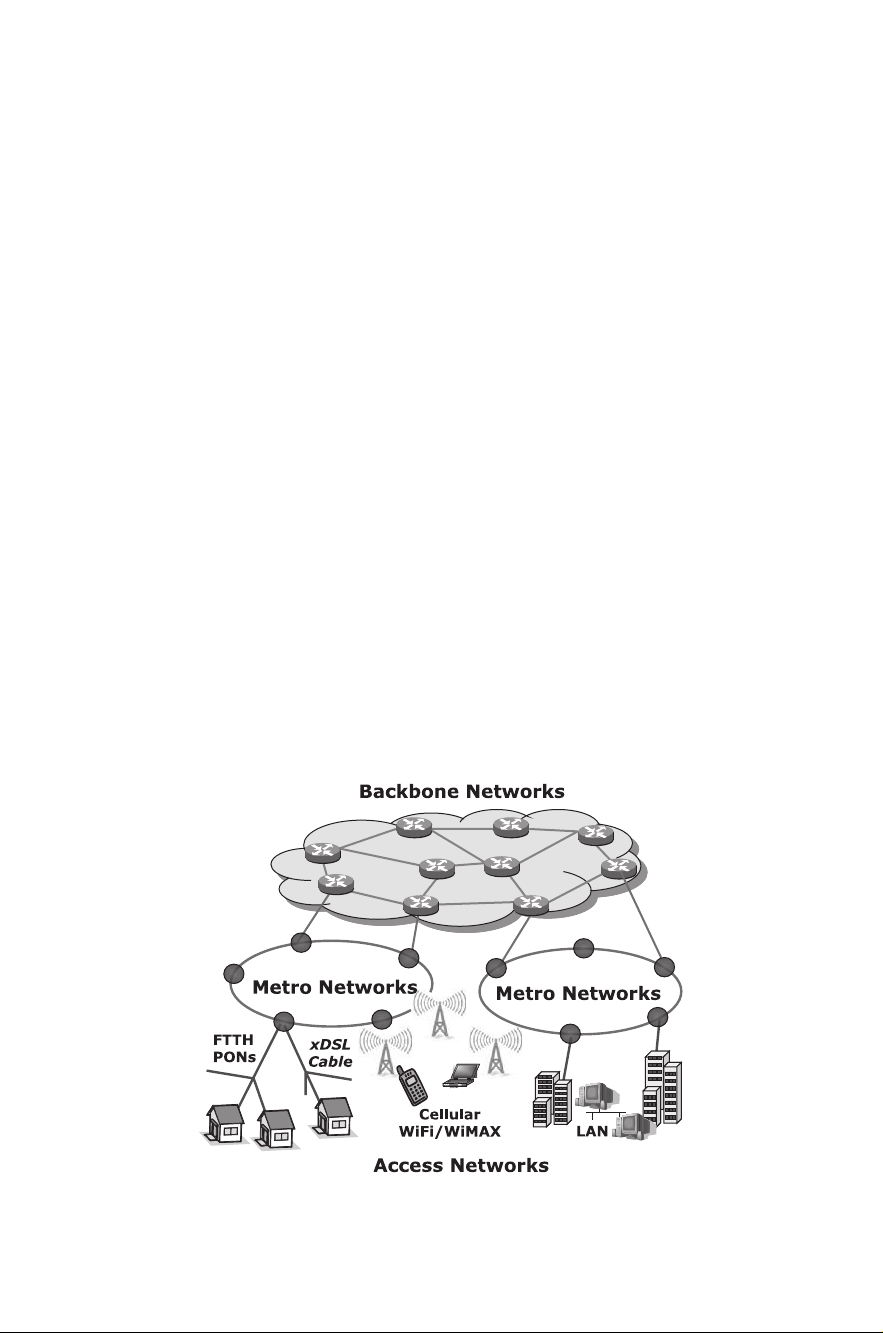
covers a very large geographic area, all over the world and even in outer space. Such
a complicated system is built and managed within a hierarchical structure, consisting
of local area, access area, metropolitan area, and wide area networks (as shown in
Figure 1.1). All the network layers cooperate to achieve the ultimate task: anyone,
anywhere, anytime, and any media communications.

Local Area Networks

Local area networks (LANs) mainly connect computers and
other electronicdevices (servers, printers,etc.) within an office, a single building, or a
few adjacent buildings. Therefore, the geographical coverage of LANs is very small,
spanning from a few meters to a few hundred meters. LANs are generally not a part
of public networks but are owned and operated by private organizations. Common

FIGURE 1.1 Hierarchical architecture of global communication infrastructure.

COMMUNICATION NETWORKS 3

topologies for LANs are bus, ring, star, or tree. The most popular LANs are parts of
the Ethernet, supporting a few hundred users with typical bit rates of 10 or 100 Mb/s.

Access Networks

The computers andother communication equipmentof a private
organization are usually connected to a public telecommunication networks through
access networks.Access networks bridge end users to service providers through twist
pairs (phone line), coaxial cables, or other leased lines (such as OC3 through optical
fiber). The typical distance covered by an access network is a few kilometers up to
20 km. For personal users, access networks use DSL or cable modem technology
with a transmission rate of a few megabits per second; for business users, networks
employ point-to-point fiber links with hundreds of megabits or gigabits per second.

Metropolitan Area Networks

Metropolitan area networks (MANs) aggregate the
traffic from access networks and transport the data at a higher speed. A typical area
covered by a MAN spans a metropolitan area or a small region in the countryside.
Its topology is usually a fiber ring connecting multiple central offices, where the
transmission data rate is typically 2.5 or 10 Gb/s.

Wide Area Networks

Wide area networks (WANs) carry a large amount of traffic
among cities, countries, and continents. MAN multiplexes traffic from LANs and
transports the aggregated traffic at a much higher data rate, typically tens of gigabits
per second or higher using wavelength-division multiplexing (WDM) technology
over optical fibers. Whereas a WAN covers the area of a nation or, in some cases,
multiple nations, a link or path through a MAN could be as long as a few thousand
kilometers. Beyond MANs, submarine links connect continents. Generally, the sub­marine systems are point-to-point links with a large capacity and an extremely long
path, from a few thousand up to 10,000 km. Because these links are designed for
ultralong distances and operate under the sea, the design requirements are much more
stringent than those of their terrestrial counterparts. Presently, submarine links are
deployed across the Pacific and Atlantic oceans. Some shorter submarine links are
also widely used in the Mediterranean, Asian Pacific, and African areas.

Service Convergence

Historically, communication networks provide mainly
three types of service: voice, data, and video (triple play). Voice conversation us­ing plain old telephony is a continuous 3.4-kHz analog signal carried by two-way,
point-to-point circuits with a very stringent delay requirement. The standard TV sig­nal is a continuous 6-MHz analog signal usually distributed with point-to-multipoint
broadcasting. Data transmission is typically bursty with varying bandwidth and de­lay requirements. Because the traffic characteristics of voice, data, and video and
their corresponding requirements as to quality of service (QoS) are fundamentally
different, three major types of networks were developed specifically to render these
services in a cost-effective manner: PSTN (public-switched telephone networks) for
voice conversation, HFC (hybrid fiber coax) networks for video distribution, and the
Internet for data transfer. Although HFC networks are optimized for video broad­casting, the inherent one-way communication is not suitable for bidirectional data or

4 BROADBAND ACCESS TECHNOLOGIES: AN OVERVIEW

voice. PSTN adopts circuit switching technology to carry information with specific
bandwidth or data rates, such as voice signals. However, circuit-switched networks
are not very efficient for carrying bursty data traffic. With packet switching, the
Internet can support bursty data transmission, but it is very difficult to meet stringent
delay requirements for certain applications. Therefore, no single network can satisfy
all the service requirements.

Emerging multimedia applications suchas videoon demand, e-learning, and inter­active gaming require simultaneous transmission of voice, data, and video. Driven by
user demands and stiff competition, service providers are moving toward a converged
network for multimedia applications, which will utilize Internet protocol (IP) tech­nologies to provide triple-play services. As VoIP (voice over IP) has been developed
in the past few years and more recently IP TV has become a mature technology,
all network services will converge into an IP-based service platform. Furthermore,
the integration of optical and wireless technologies will make quadruple play (voice,
data, video, and mobility) a reality in the near future.

1.2 ACCESS TECHNOLOGIES

Emerging multimedia applications continuously fuel the explosive growth of the
Internet and gradually pervade every area of our lives, from home to workplace. To
provide multimedia service to every home and every user, access networks are built
to connect end users to service providers. The link between service providers and
end users is often called the last mile by service providers, or from an end user’s
perspective, the first mile. Ideally, access networks should be a converged platform
capable of supporting a variety of applications and services. Through broadband
access networks, integrated voice, data, and video service are provided to end users.
However, the reality is that access networks are the weakest links in the current
Internet infrastructure. While national information highways (WANs and MANs)
have been developed in most parts of the globe, ramps and access routes to these
information highways (i.e.,the first/lastmile) are mostlybike lanes or at best,unpaved
roads, causing traffic congestion. Hence, pervasive broadband access should be a
national imperative for future Internet development. In this section we review current
access scenarios and discuss the last-mile bottleneck and its possible solutions.

1.2.1 Last-Mile Bottleneck

Due to advances in photonic technologies and worldwide deployment of optical
fibers, during the last decade the telecommunication industry has experienced an ex­traordinary increase in transmission capacity in core transport networks. Commercial
systems with 1-Tb/s transmission can easily be implemented in the field, and the
state-of-the-art fiber optical transmission technology has reached 10 Tb/s in a single
fiber. In the meanwhile, at the user end, the drastic improvement in the performance
of personal computers and consumer electronic devices has made possible expand­ing demands of multimedia services, such as video on demand, video conferencing,

ACCESS TECHNOLOGIES 5

TABLE 1.1 Multimedia Applications and Their Bandwidth Requirements

Application Bandwidth Latency Other Requirements

Voice over IP (VoIP) 64 kb/s 200 ms Protection
Videoconferencing 2 Mb/s 200 ms Protection
File sharing 3 Mb/s 1 s
SDTV 4.5 Mb/s/ch 10 s Multicasting
Interactive gaming 5 Mb/s 200 ms
Telemedicine 8 Mb/s 50 ms Protection
Real-time video 10 Mb/s 200 ms Content distribution
Video on demand 10 Mb/s/ch 10 s Low packet loss
HDTV 10 Mb/s/ch 10 s Multicasting
Network-hosted software 25 Mb/s 200 ms Security

e-learning, interactive games, VoIP, and others. Table 1.1 lists common end-user ap­plications and their bandwidth requirements. As a result of the constantly increasing
bandwidth demand,users may require more than 50 Mb/s in the near future. However,
the current copper wire technologies bridging users and core networks have reached
their fundamental bandwidth limits and become the first-last-mile bottleneck. Delays
in Web page browsing, data access, and audio/video clip downloading have earned
the Internet the nickname “World Wide Wait.” How to alleviate this bottleneck has
been a very challenging task for service providers.

1.2.2 Access Technologies Compared

For broadband access services, there is strong competition among several technolo­gies: digital subscriber line, hybrid fiber coax, wireless, and FTTx (fiber to the x,
x standing for home, curb, neighborhood, office, business, premise, user, etc.). For
comparison, Table 1.2 lists the bandwidths (per user) and reaches of these com­peting technologies. Currently, dominant broadband access technologies are digital

TABLE 1.2 Comparison of Bandwidth and Reach for Popular Access Technologies

Service Medium Downstream (Mb/s) Upstream (Mb/s) Max Reach (km)

ADSL Twisted pair 8 0.896 5.5
ADSL2 Twisted pair 15 3.8 5.5
VDSL1 Twisted pair 50 30 1.5
VDSL2 Twisted pair 100 30 0.5
HFC Coax cable 40 9 25

BPON Fiber 622 155 20
GPON Fiber 2488 1244 20
EPON Fiber 1000 1000 20

Wi-Fi Free space 54 54 0.1
WiMAX Free space 134 134 5

6 BROADBAND ACCESS TECHNOLOGIES: AN OVERVIEW

subscriber loop and coaxial cable. For conventional ADSL (asymmetric DSL) tech­nology, the bandwidth available is a few Mb/s within the 5.5-km range. Newer VDSL
(very high-speed DSL) can provide 50 Mb/s, but the maximum reach is limited to

1.5 km. On the other hand, coaxial cable has a much larger bandwidth than twist
pairs, which can be as high as 1 Gb/s. However, due to the broadcast nature of CATV
system, current cable modems can provide each user with an average bandwidth of a
few Mb/s. While DSL and cable provide wired solutions for broadband access, Wi-Fi
(wireless fidelity), and WiMAX (worldwide interoperability for microwave access)
provide mobile access in a LAN or MAN network. Even though a nominal band­width of Wi-Fi andWiMAX can be relatively higher(54 Mb/s in 100 mfor Wi-Fi and
28 Mb/s in 15 km for WiMAX), the reach of such wireless access is very limited and
the actual bandwidth provided to users can be much lower, due to the interference in
wireless channels. As a LAN technology, the primary use of Wi-Fi is in home and of­fice networking. To reach the central office or service provider, multiple-hop wireless
links with WiMAX have to be adopted. An alternative technology that is also under
development is MBWA (mobile broadband wireless access, IEEE 802.20), which is
very similar to WiMAX (IEEE 802.16e). Compared to the fixed access solutions,
the advantages of the wireless technologies are easy deployment and ubiquitous or
mobile access, and the disadvantages are unreliable bandwidth provisioning and/or
limited access range.

The bandwidth and/or reach of the copper wire and wireless access technology is
very limited due to the physical media constraints. To satisfy the future use demand
(>30 Mb/s), there is a strategic urgency for service providers to deploy FTTx net­works. Currently, for cost and deployment reasons, FTTx is competing with other
access technologies. Long term, however, only optical fiber can provide the unlim­ited capacity and performance that will be required by future broadband services.
FTTx has long been dubbed as a future-proof technology for the access networks.
A number of optical access network architectures have been standardized (APON,
BPON, EPON, and GPON), and cost-effective components and devices for FTTx
have matured. We are currently witnessing a worldwide deployment of optical access
networks and a steady increase in FTTx users.

1.3 DIGITAL SUBSCRIBER LINE

Digital subscriber line (also called digital subscriber loop) is a family of access
technologies that utilize the telephone line (twisted pair) to provide broadband access
service. While the audio signal (voice) carried by a telephony system is limited from
300 to 3400 Hz, the twisted pair connecting the users to the central office is capable
of carrying frequencies well beyond the 3.4-kHz upper limit of the telephony system.
Depending on the length and the quality of the twisted pair, the upper limit can
extend to tens of megahertz. DSL takes advantage of this unused bandwidth and
transmits data using multiple-frequency channels. Thus, some types of DSL allow
simultaneous use of the telephone and broadband access on the same twisted pair.

DIGITAL SUBSCRIBER LINE 7

Modem

Central

Office

FIGURE 1.2 DSL access networks.

Figure 1.2 shows the typical setup of a DSL configuration. At the central office, a
DSLAM (DSL access multiplexer) sends the data to users via downstream channels.
At the user side, a DSL modem functions as a modulator/demodulator (i.e., receives
data from DSLAM and modulates user data for upstream transmission).

1.3.1 DSL Standards

DSL comes indifferent flavors, supporting various downstream/upstream bit rates and
access distances. DSLstandards are defined inANSI T1, andITU-T Recommendation
G.992/993. Table 1.2 lists various DSL standards and their performance. Collectively,
these DSL technologies are referred to as xDSL. Two commonly deployed DSL
standards are ADSL and VDSL.

As its namesuggests, ADSLsupports asymmetrical transmission.Since the typical
ratio of traffic asymmetry is about 2 :1 to 3 : 1, ADSL becomes a popular choice for
broadband access. In addition, there is more crosstalk from other circuits at the
DSLAM end. As the upload signal is weak at the noisy DSLAM end, it makes sense
technically to have upstream transmission at a lower bit rate. Depending on thelength
and quality (such as the signal-to-noise ratio) of the twisted pair, the downstream bit
rate can be as high as 10 times the upstream transmission. The maximum reach of
ADSL is 5500 m. While ADSL1 can support a downstream bit rate up to 8 Mb/s and
an upstream data rate up to 896 kb/s, ADSL2 supports up to 15 Mb/s downstream
and 3.8 Mb/s upstream.

To support higherbit rates, theVDSL standard wasdevelopedafter ADSL. Trading
transmission distance fordata rate, VDSLcan support amuch higher datarate but with
very limited reach. VDSL1 standards specify data rates of 50 Mb/s for downstream
and 30 Mb/s for upstream transmission. The maximum reach of VDSL1 is limited
to 1500 m. The newer version of VDSL standards, VDSL2, is an enhancement of

8 BROADBAND ACCESS TECHNOLOGIES: AN OVERVIEW

VDSL1, supporting a data rate up to 100 Mb/s (with a transmission distance of
500 m). At 1 km, the bit rate will drop to 50 Mb/s. For reaches longer than 1.6 km,
the VDSL2 performance is close to ADSL. Because of its higher data rates and
ADSL-like long reach performance, VDSL2 is considered to be a very promising
solution for upgrading existing ADSL infrastructure.

ADSL and VDSL are designed for residential subscribers with asymmetric band­width demands. For business users, symmetrical connections are generally required.
Two symmetrical DSL standards, HDSL and SHDSL, aredeveloped for businesscus­tomers. While HDSL supports a T1 line data rate at 1.552 Mb/s (including 8 kb/s of
overhead) with a reach of about 4000 m, SHDSL can provide a 6.696-Mb/s data rate
with a maximum reach of 5500 m. However, HDSL and SHDSL do not support si­multaneous telephone service, as most business customers do not have a requirement
for a simultaneous voice circuit.

1.3.2 Modulation Methods

DSL uses a DMT (discrete multitone) modulation method. In DMT modulation,
complex-to-real inverse discrete Fourier transform is used to partition the available
bandwidth of the twisted pair into 256 orthogonal subchannels. DMT is adaptive to
the quality of the twisted pair, so all the available bandwidth is fully utilized. The
signal-to-noise ratio of each subchannel is monitored continuously. Based on the
noise margin and bit error rate, a set of subchannels are selected, and a block of data
bits are mapped into subchannels. In each subchannel, QAM (quadrature amplitude
modulation) with a 4-kHz symbol rate is used to modulate the bit stream onto a
subcarrier, leading to 60 kb/s per channel. Typically, the frequency range between 25
and 160 kHz is used for upstream transmission, and 140 kHz to 1.1 MHz is used for
downstream transmission.

1.3.3 Voice over DSL

DSL was designed originally to carry data over phone lines, and DSL signal is
separated from voice signal. Recently, new protocols have been proposed to merge
voice and data at the circuit level. With advanced coding technologies, a 64-kb/s
digitized voice signal can be compressed to 8 kb/s or less, thus allowing more voice
channels to be carried over the same phone line. A voice over a DSL (VoDSL)
gateway converts and compresses the analog voice signal to digital bit streams, so
that calls made over VoDSL are indistinguishable from conventional calls. Usually,
12 to 20 voice channels can be carried over a single DSL line, depending on the
transmission distance and the signal quality. A VoDSL system can be integrated
into higher-layer protocols such as IP and ATM. Early DSL networks used ATM
to ensure QoS, where ATM virtual circuits were used for the voice traffic. ADSL
and VDSL networks migrate to packet-based transport, and they use packet-switched
based virtual circuits instead of ATM ones.

HYBRID FIBER COAX 9

1.4 HYBRID FIBER COAX

Cable networks were originally developed for a very simple reason: TV signal dis­tribution. Therefore, cable networks are optimized for one-way, point-to-multipoint
broadcasting of analog TV signals. As optical communication systems were devel­oped, most cable TV systems have gradually been upgraded to hybrid fiber coax
(HFC) networks, eliminating numerous electronic amplifiers along the trunk line.
However, before cable access technology can be deployed, a return pass must be
implemented for upstream traffic. To support two-way communication, bidirectional
amplifiers have to be used in HFC systems, where filters are deployed to split the
upstream (forward) and downstream (reverse) signals for separate amplification.

Figure 1.3 presents the network architecture of a typical HFC network. In HFC
networks, analog TV signals are carried from the cable headend to distribution nodes
using optical fibers, and from the distribution node, coaxial cable drops are deployed
to serve 500 to 2000 subscribers. As shown in the figure, an HFC network is a shared
medium system with a tree topology.In sucha topology, multiple users share the same
HFC infrastructure, so medium access control is required in upstream transmission
while downstream transmission uses a broadcast scheme. A cable modem deployed
at the subscriber end provides data connection to the cable network, while at the
headend, the cable modem termination system connects to a variety of data servers
and provides service to subscribers.

Compared withthe twisted pairs in a telephone system, coaxial cables have amuch
higher bandwidth (1000 MHz), thus can support a much higher data rate. Depending
on the signal-to-noise ratio on the coaxial cable, 40 Mb/s can be delivered to the
end users with QAM modulation. For upstream transmission, QPSK can deliver up
to a 10-Mb/s data rate. However, as cable systems are shared-medium networks, the
bandwidth is thus shared by all the cable modems connected to the network. By
contrast, DSL uses dedicated twist pairs for each user, thus no bandwidth sharing
for different users. Furthermore, as the transmission bandwidth must be shared by
multiple users, medium access control protocol must be deployed to govern upstream
transmission. If congestion occurs in a specific channel, the headend must be able to
instruct cable modems to tune its receiver to a different channel.

Primary

hub

Master

headend

FIGURE 1.3 HFC access networks.

Secondary

hub

Fiber
node

RF amplifier

10 BROADBAND ACCESS TECHNOLOGIES: AN OVERVIEW

1.4.1 Cable Modem

Cable modems were developed to transport high-speed data to and from end users
in an HFC network. Traditional TV broadcasting occupies frequencies up to 1 GHz,
with each TV channel occupying 6 MHz of bandwidth (Part 76 in the FCC rules). A
cable modem uses two of those 6-MHz channels for data transmission. For upstream
transmission, a cable modem sends user data to the headend using a 6-MHz band
between 5 and 42 MHz. At the same time, the cable modem must tune its receiver to
a 6-MHz band within a 450- to 750-MHz band to receive downstream data. While a
QAM modulation scheme is used for downstream data, a QPSK modulation scheme
is usuallyselected for upstream transmission, as it is more immune to the interference
resulting from radio broadcasting.

1.4.2 DOCSIS

DOCSIS (Data Over Cable Service Interface Specifications), developed by Cable­Labs, a consortiumofequipment manufactuers, isthecurrent standard forcableaccess
technology. DOCSIS defines the functionalities and properties of cable modems at a
subscriber’s premises and cable modem termination systems at the headend. As its
name suggests, DOCSIS specifies the physical layer characteristics, such as trans­mission frequency, bit rate, modulation format, and power levels, of cable modem
and cable modem termination systems, but also the data link layer protocol, such as
frame structure, medium access control, and link security. Three different versions of
DOCSIS (1.0/2.0/3.0) was developed during the past decade and were later ratified
as ITU-T Recommendation J.112, J.122, and J.222. Although some compromise is
needed as cable networks are a shared medium, DOCSIS offers various classes of
service with medium access control. Such QoS features in DOCSIS can support
applications (such as VoIP) that have stringent delay or bandwidth requirements.

Physical Layer

The upstreamPMD layersupports twomodulation formats:QPSK
and 16-QAM, and the downstream PMD layers uses 64-QAM and 256-QAM. The
nominal symbol rate is 0.16, 0.32, 0.64, 1.28, 2.56, or 5.12 Mbaud. Therefore, the
maximum downstream data rate is about 40 Mb/s and the upstream data rate is
about 20 Mb/s. To mitigate the effect of noise and other detrimental channel effects,
Reed–Solomon encoding, transmitter equalizer, and variable interleaving schemes
are commonly used.

Data Link Layer

The DOCSIS data link layer specifies frame structure, MAC, and
link security. The frame structure used in HFC networks isvery similar to the Ethernet
in both the upstream and downstream directions. For the downstream direction, data
frames are embedded in 188-byte MPEG-2 (ITU-T H.222.0) packets with a 4-byte
header followed by 184 bytes of payload. Downstream uses TDM transmission
schemes, synchronous to all modems. In the upstream direction, TDMA or S-CDMA
are defined for medium access control. An upstream packet includes physical layer
overhead, a unique word, MAC overhead, packet payload, and FEC bytes. MAC

OPTICAL ACCESS NETWORKS 11

layer specifications also include modem registration, ranging, bandwidth allocation,
collision detection and contention resolution, error detection, and data recovery. An
access security mechanism in DOCSIS defines a baseline privacy interface, security
system interface, and removable security module interface, to ensure information
security in HFC networks.

1.5 OPTICAL ACCESS NETWORKS

Due to their ultrahigh bandwidth and low attenuation, optical fibers have been widely
deployed for wide area networks and metro area networks. To some extent, mul­timode fibers were also deployed in office buildings for local area networks. Even
though optical fibers are ideal media for high-speed communication systems and net­works, the deployment cost was considered prohibitive in the access area, and copper
wires still dominate in the current marketplace. However, as discussed in Section 1.2,
emerging multimedia applications have created such large bandwidth demands that
copper wire technologies have reached their bandwidth limits. Meanwhile, low-cost
photonic components and passive optical network architecture have made fiber a
very attractive solution. In the past few years, various PON architecture and tech­nologies have been studied by the telecom industry, and a few PON standards have
been approved by ITU-T and IEEE. FTTx becomes a mature technology in direct
competition with copper wires. In fact, large-scale deployment has started in Asia,
North America, and Europe, and millions of subscribers are enjoying the benefit of
PON technologies.

1.5.1 Passive Optical Networks

Figure 1.4 illustrates the architecture of a passive optical network. As the name
implies, there is no active componentbetween the central office andthe user premises.
Active devices exist only in the central office and at user premises. From the central
office, a standardsingle-mode opticalfiber (feeder fiber) runs toa 1 : N passiveoptical
power splitter near the user premises. Theoutput ports of the passive splitterconnects
to the subscribers through individual single-mode fibers (distribution fibers). The
transmission distance in a passive optical networks is limited to 20 km, as specified
in current standards. The fibersand passive components between the centraloffice and
users premises are commonly called an optical distribution network. The number of
users supported by a PON can be anywhere from 2 to 128, depending on thethe power
budget, but typically, 16, 32,or 64.At the central office, anoptical lineterminal (OLT)
transmits downstream data using 1490-nm wavelength, and the broadcasting video is
sent through 1550-nm wavelength. Downstream uses a broadcast and select scheme;
that is, thedownstream data andvideo are broadcast to eachuser with MAC addresses,
and the user selects the data packet–based MAC addresses. At the user end, an
optical network unit(ONU), also called an optical network terminal (ONT), transmits
upstream data at 1310-nm wavelength. To avoidcollision, upstreamtransmission uses
a multiple access protocol (i.e., time-division multiple access) to assign time slots to

12 BROADBAND ACCESS TECHNOLOGIES: AN OVERVIEW

TDM PON Standards
BPON: ITU G.983
GPON: ITU G.984
EPON: IEEE 802.3ah

10 ~ 20 km

ONU

Fiber to the office/business

OLT

Central Office

OLT: Optical Line Terminal
ONU: Optical Network Unit

Coupler

FIGURE 1.4 Passive optical networks.

ONU

Fiber to the node/curb/neighborhood

VDSL, WiFi, etc.

ONU

Fiber to the home/user

each user. This type of passive optical network is called TDM PON. The ONU could
be located in a home, office, a curbside cabinet, or elsewhere. Thus comes the so­called fiber-to-the-home/office/business/neighborhood/curb/user/premises/node, all
of which are commonly referred to as fiber to the x. In the case of fiber-to-the-
neighborhood/curb/node, twisted pairs are typically deployed to connect end users to
the ONUs, thus providing a hybrid fiber/DSL access solution.

1.5.2 PON Standard Development

Early work of passive optical networks started in 1990s, when telecom service
providers and system equipment vendors formed the FSAN (full service access
networks) working group. The common goal of the FSAN group is to develop truly
broadband fiber access networks. Because of the traffic management capabilities
and robust QoS support of ATM (asynchronous transfer mode), the first PON stan­dard, APON, is based on ATM and hence referred to as ATM PON. APON supports

622.08 Mb/s for downstream transmission and 155.52 Mb/s for upstream traffic.
Downstream voice and data traffic is transmitted using 1490-nm wavelength, and
downstream video is transmitted with 1550-nm wavelength. For upstream, user data
are transmitted with 1310-nm wavelength. All the user traffic is encapsulated in
standard ATM cells, which consists of 5-byte control header and 48-byte user data.
APON standard was ratified by ITU-T in 1998 in Recommendation G.983.1. In the
early days, APON was most deployed for business applications (e.g., fiber-to-the­office). However,APON networksare largely substitutedwith higher-bit-rate BPONs
and GPONs.

OPTICAL ACCESS NETWORKS 13

Based on APON, ITU-T further developed BPON standard as specified in a series
of recommendations in G.983. BPON is an enhancement of APON, where a higher
data rate and detailed control protocols are specified. BPON supports a maximum
downstream data rate at 1.2 Gb/s and a maximum upstream data rate at 622 Mb/s.
ITU-T G.983 also specifies dynamic bandwidth allocation (DBA), management and
control interfaces, and network protection. There has been large-scale deployment of
BPON in support of fiber-to-the-premises applications.

The growing demand for higher bandwidth in the access networks stimulated
further development of PON standards with higher capacity beyond those of APON
and BPON. Starting in 2001, the FSAN group developed a new standard called
gigabit PON,which becomes the ITU-T G.984 standard. The GPON physical media–
dependent layer supports a maximum downstream/upstream data rate at 2.488 Gb/s,
and thetransmission convergencelayer specifies a GPON frame format, media access
control, operation and maintenance procedures, and an encryption method. Based
on the ITU-T G.7041 generic framing procedure, GPON adopts GEM (a GPON
encapsulation method) to support different layer 2 protocols, such as ATM and
Ethernet. The novel GEM encapsulation method is backwardly compatible with
APON and BPONandprovides better efficiencythan do Ethernetframes. Deployment
of GPON hadtaken off in North America andlargelyreplaced older BPONsand more.

While ITU-T rolled out BPON and GPON standards, IEEE Ethernet-in-the-first­mile working group developed a PONstandardbased on Ethernet.The EPON physical
media–dependent layer can support maximum1.25-Gb/s (effectivedata rate1.0 Gb/s)
downstream/upstream traffic. EPON encapsulate and transport user data in Ethernet
frames. Thus, EPON is a natural extension of the local area networks in the user
premises, andconnects LANsto theEthernet-based MAN/WAN infrastructure. Since
there is nodata fragment orassembly in EPON andits requirement onphysical media–
dependent layer is more relaxed, EPON equipment is less expensive than GPON. As
Ethernet has beenused widely inlocal areanetworks,EPON becomesa very attractive
access technology. Currently, EPON networks have been deployed on a large scale
in Japan, serving millions of users.

1.5.3 WDM PONs

As the user bandwidth demands keep increasing, current GPON or EPON will even­tually no longer be able to satisfy the bandwidthrequirement. Thereare a few possible
solutions. One possibility is to split a single PON into multiple PONs so that each
PON supports fewer users and each user gets more bandwidth. Another alternative
is to use a higher bit rate, such as 10 Gb/s. In fact, an IEEE 802.3av study group
is creating a draft standard on 10-Gb/s EPON. However, both solutions for higher
bandwidth (i.e., higher bit rate or fewer users per PON) are not very cost-effective
and do not scale very well as the bandwidth demands increase further. Inaddition, the
power distribution of the passive splitter is fixed; that will lead to an uneven power
budget for users and limit the transmission distance. Ultimately, WDM PON is the
only future proof of technology that can satisfy any bandwidth demands.

14 BROADBAND ACCESS TECHNOLOGIES: AN OVERVIEW

TX

1

OLT

ONU

1

TX

1

RX

TX

RX

1

Fiber

32

32

MUX

DEMUX

MUX

DEMUX

ONU

32

RX

TX

RX

1

32

32

FIGURE 1.5 WDM passive optical networks.

Figure 1.5 shows the network architecture of WDM PONs. Transmitters with
varying wavelengths will be deployed at the OLT and ONU sides, and a passive
wavelength-division multiplexer will be inserted at the distribution node to separate
and combine multiple wavelengths. Thus, the fiber distribution network will be kept
passive.If the user bandwidthdemands are notverylarge,or in theotherwords, a small
number of users can still share asingle wavelength, a passive power splitterfollowing
the WDM is used to broadcast the downstream traffic and combine the upstream
traffic. In this case, multiple wavelengths separate a single PON into multiple logical
TDM PONs. Each PON runs on a different wavelength, and fewer users share the
bandwidth of a TDM PON. In addition, since the optical power is split for a smaller
number of users, WDM PONs is less subject to optical power budget constraints,
leading to long-reach access networks. If a user requires a large amount of bandwidth
(e.g., a few gigabits per second), a single wavelength can be provided for this specific
user; or in an extreme case, multiple wavelengths, hence a large bandwidth, can be
provided to a single user if needed.

In WDM PONs, the equipment and resources at OLT are shared by fewer users,
leading to higher cost per user. Hence, WDM PONs are considered much more ex­pensive than TDM PONs. However, to support high-bandwidth applications, there
will be a need in the near future to move from TDM access networks to WDM
access networks. Currently, the way to migrate from current TDM access networks
to WDM access networks in a cost-effective, flexible, and scalable manner is not at
all clear. A method to upgrade the access service smoothly and cost-effectively from
a current TDM FTTx network to a future WDM FTTx network with a minimum
influence on legacy users is the object of intense research. Various approaches to
implementing WDM have been and are being explored, and field deployment has
begun in Asia (South Korea, to be exact). A number of schemes to incorporate WDM
technology into access networks have been studied and tested in experiments, and
the WDM FTTx network architecture exhibits certain exceptional features in the
WDM implementation in either downstream, upstream, or both directions. As optical

OPTICAL ACCESS NETWORKS 15

technology becomes cheaper and easier to deploy and end users demand ever­increasing bandwidth, WDM PONs will eventually make the first/last-mile bottle­neck history.

1.5.4 Other Types of Optical Access Networks

In addition to the passive optical networks, TDM and WDM PONs, that we have
discussed, other types of optical access networks have been developed over the
years, including Ethernet over fiber, DOCSIS PON, RF PON, and free-space optical
networks. Ethernet over fiber is essentially point-to-point Ethernet built on fiber links.
DOCSIS and RF PON is two flavors of PON developed for cable companies. Free­space optical networks is a wireless access solution utilizing optical communication
technologies.

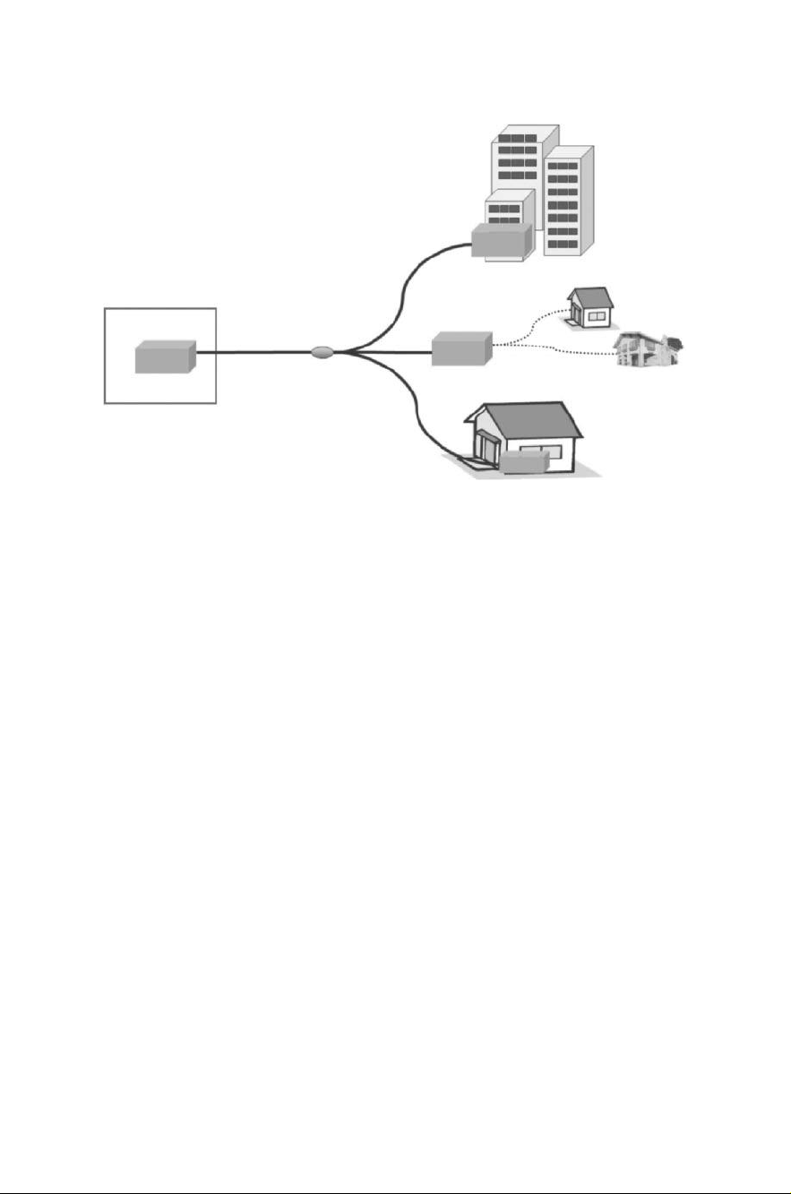
Ethernet over Fiber

Ethernet over fiber is deployed primarily in point-to-point
topology. Typically, dedicated fiber connects a subscriber to the central office,
and each subscriber requires two dedicated transceivers (one at the user premises and
the other at the central office). This approach requires a large number of fibers and
optical transceivers and thus incurs a large cost associated with fiber and equipment.
Since each fiber link can run on its full capacity, Ethernet over fiber, which requires
gigabit bandwidth, is used primarily for business subscribers. Figure 1.6 shows an

Ethernet

switch

Central

office

FIGURE 1.6 Point-to-point Ethernet optical access networks.

16 BROADBAND ACCESS TECHNOLOGIES: AN OVERVIEW

alternative architecture for Ethernet over fiber. A local Ethernet switch is deployed to
the user sites. Individual fiber can then run from the switch to each user, and only a
single fiber (bidirectional) or two fibers (unidirectional) connect the Ethernet switch
to the central office. This approach reduces the number of fibers run from the central
office but requires an active Ethernet switch in the field and requires at least two more
transceivers than is the case on the left in the figure.

DOCSIS PON

While telecom companies are deploying PONs worldwide on a
large scale, MSOs (multisystem operators) need to upgrade their fiber coax systems
to compete in FTTx markets. DOCSIS PON, or DPON, is developed to provide
a DOCSIS service layer interface on top of PON architecture. DPON implements
DOCSIS functionalities, including OAMP (operation, administration, maintenance,
and provisioning) on existing PON systems, and thus allow MSOs to use set-top
and DOCSIS equipment located in homes and headends over PONs. However, fun­damentally, DPON service is based on current EPON or GPON MAC and phys­ical layer standards. Therefore, DPON is just an application running on top of
PON systems.

RF PON

Radio-frequency PON (RF PON) is another flavor of passive optical
networks developed for MSOs. RF PONs support RF video broadcasting signals
over optical fibers. As MSOs expand the network footprint and launch new prod­ucts using additional RF bandwidth, more active RF components are deployed and
higher frequenciessometimes requireRF electronicschange-outs and respacing. As a
consequence, HFC networks experience reduced signal quality, lower reliability, and
higher operating and maintenance cost. RF PONs are a natural evolution of current
HFC networks, as they offer backward compatibility with current RF video broad­casting technologies and provides significant cost reduction in network operation and
maintenance.

OCDM PON

Optical code-division multiplexing (OCDM) has been demonstrated
recently as an alternative multiplexing technique for PONs. Similar to electronic
CDMA technology, users in OCDM PONs are assigned orthogonal codes with which
each user’s data are encoded or decoded into or from optical pulse sequence. OCDM
PONs can thus provide asynchronous communications and security against unautho­rized users. However, the optical encoders and decoders for OCDM are expensive,
and the number of users is limited by interference and noise.

Free-Space Optical Networks

Unlike fiber opticcommunications, free-space op-

tical communication (also called optical wireless communication) uses atmosphere

as the communication medium. This is probably one of the old long-distance com­munication methods (e.g., smoke signals) used a few thousands years ago. During
the past decades, there has been revived interest in free-space communication for
satellite and urban environment. Particularly in the access networks, it can used to
connect a subscriber directly to a central office. Figure 1.7 shows a typical setup

OPTICAL ACCESS NETWORKS 17

FIGURE 1.7 Free-space optical communicationsand networks. Point-to-pointoptical wire­less links on the roofs of buildings form a mesh network for broadband access.

for urban free-space optical communication networks. Due to the line-of-sight re­quirement for free-space optical communications, optical transceivers are usually
mounted on the tops of buildings, and telescopes are typically used in the transmitter
to improve the alignment of optical links. Multiple point-to-point links can form a
mesh network, improving its scalability and reliability. As a wireless technology,
the cost of free-space optical communication is very low, about 10% of fiber optic
communications, and the high-speed link can be set up and torn down in a couple
hours. Compared to other wireless access technologies, it provides a higher data
rate, longer reach, and better signal quality. So far, thousands of free-space optical
links have beendeployed. However,atmosphere is not an idealtransmission medium,
due to attenuation and scattering at optical frequency. Turbulence, rain, and dense
fog could be very challenging for free-space optical communication. For long-reach
links, alignment of optical transmitters and receivers is also difficult, and an adaptive
ray-tracking system might be needed for rapid pointing and accurate alignment. Po­tentially, survivable network topology, transmitter and receiver arrays, and adaptive
and equalization technologies could help mitigate the atmospheric effect and align­ment problem. Integration with wire line networks such as PONscan greatly improve
the reliability and survivability of free-space optical access networks. In the future,
we may witness more and more free-space optical networks in urban settings.

18 BROADBAND ACCESS TECHNOLOGIES: AN OVERVIEW

1.6 BROADBAND OVER POWER LINES

Ac power lines have long been considered a workable communication medium. For
decades, utility companies have used power lines for signaling and control, but they
are used primarily for internal management of power grids, household intercoms, and
lighting controls. As deregulation of both the telecom and electricity industries was
unfolding in the 1990s, broadband access over power lines became a possibility. As
power lines reach more residences than does any other medium, significant efforts
have been madeto develop high-speedaccess over power lines.A number of solutions
have been proposed and tested in the field. Even though DSL or cable currently
dominates the broadband access services, and PONs are very promising for the near
future, broadbandover power lines (BPL) can stillclaim itspart in the current market.
For example, in some rural areas, building infrastructure to provide DSL or cable
could be very expensive, while power-line communications could easily provide
broadband services. Anywhere there is electricity there could be broadband over
power lines. In addition, there is a great potential to network all the appliances in a
household through the power line, thus providing a smart home solution. However,
at present power-line communication technology and its market potential remain to
be developed further.

1.6.1 Power-Line Communications

Figure 1.8 shows the topology of the electrical power distribution grid. The three­phase power generated at a power plant enters a transmission substation, where the
three-phase power generated by the power generators is converted to extremely high

Power

Plant

Power

Substation

High-Voltage

Transmission Lines

Distribution

Lines

FIGURE 1.8 Electrical power transmission and distribution.

Powe rline

substation

BROADBAND OVER POWER LINES 19

Coupler

& Bridge

FIGURE 1.9 Broadband power-line communications.

voltages (155 to 765 kV) for long-distance transmission over the grid. Within the
transmission grid, many power substations convert the extremely high transmission
voltage down to distribution voltages (less than 10 kV), and this medium-voltage
electricity is sent through a bus that can split the power in multiple directions. Along
the distribution bus, there are regulator banks that regulate the voltage on the line
to avoid overshoot or undershoot, and taps that send electricity down the street. At
each building or house, there is a transformer drum attached to the electricity pole,
reducing the medium voltage (typically, 7.2 kV) to household voltage (110 or 240V).

Broadband over power lines utilizes the medium-voltage power lines to transmit
data to and from each house, as shown in Figure 1.9. Typically, repeaters are installed
along the power lines for long-distance data transmission, and some bypass devices
allow RF signals to bypass transformers. In the last step of data transmission, the
signals can be carried to each house by the power line or, alternatively, using Wi-Fi
or other wireless technology for last-mile connection.

1.6.2 BPL Modem

A BPL modem plugs into a common power socket on the wall, sending and re­ceiving data through a power line. On the other end, the BPL modem connects to
computers or other network devices by means of Ethernet cables. In some cases,
a wireless router can be integrated with a BPL modem. BPL modems transmit at
medium to high frequencies, from a few megahertz to tens of megahertz. Typical

20 BROADBAND ACCESS TECHNOLOGIES: AN OVERVIEW

data rates supported by a BPL modem range from hundreds of kilobits per second to
a few megabits per second. Various modulation schemes can be used for power-line
communications, including the older ASK (amplitude shift keying), FSK (frequency
shift keying) modulation and newer DMT, DSSS (direct sequence spread spectrum)
and OFDM(orthogonal frequency-division multiplexing) technologies. DMT, DSSS,
or OFDM modulation is perferred in modern BPL modems, as it is more robust in
handling interference and noise. Recent research has demonstrated a gigabit data rate
over power lines using microwave frequencies via surface wave propagation. This
technology can avoid the interference problems very common in power lines.

1.6.3 Challenges in BPL

BPL is a promising technology, but its development is relatively slow compared with
DSL and cable. There are a number of technical challenges that must be overcome. A
powerline is nota very goodmedium for datatransmission: Various transformers used
in the electric grid do not pass RF signals, the numerous sources of signal reflections
(impedance mismatches and lack of proper impedance termination) on power lines
hinder data transmission, and noise from numerous sources (such as power motors)
contaminates the transmission spectrum. Since power lines consist of untwisted and
unshielded wire, their long length makes them large antennas emitting RF signals and
interfering with other radio communications. Furthermore, a power line is a shared
medium limiting the bandwidth delivered to each user and raising security concerns
for private communications. All these issues have to be fully addressed before large­scale deployment can be implemented. Fortunately, much progress has been made
through intensive research during recent decades. BPL is poised to be a promising
technology for entry into the current highly competitive market.

1.7 WIRELESS ACCESS TECHNOLOGIES

Starting with RF communication and broadcasting, wireless communication tech­nologies have had an incredibly powerful effect on the entire world since the be­ginning of the twentieth century. Nowadays, AM/FM radio and TV broadcasting
blanket every continent except Antarctica; wireless cellular networks provide voice
communication to hundreds of millions of users; satellites provide video broadcast­ing and communication links worldwide; and Bluetooth and wireless LANs support
mobile services to individuals. Wireless networks are everywhere. The popularity of
wireless technologies is due primarily to their mobility, scalability, low cost, and ease
of deployment. Wireless technologies will continue to play an important part in our
daily lives, and fourth-generation wireless networks will be able to provide quadru­ple play through seamless integration of a variety of wireless networks, including
wireless personal networks, wireless LANs, wireless access networks, cellular wide
area networks, and satellite networks. In recent years, a number of wireless technolo­gies have been developed as alternatives to traditional wired access service (DSL,
cable, and PONs). Except for free-space optical communications (Section 1.5), most

WIRELESS ACCESS TECHNOLOGIES 21

wireless access networks use RF signals to establish communication links between
a central office and subscribers. In this section we discuss various broadband radio
access technologies and their characteristics. The choice of radio access technologies
depends largely on the applications, required data rate, available frequency spectrum,
and transmission distance. Even though wireless access networks cannot compete
with wired access technologies in terms of data rate and reliability, they offer flexi­bility and mobility that no other technologies can provide. Therefore, wireless access
networks complement current wired access technologies and will continue to grow
in the future.

1.7.1 Wi-Fi Mesh Networks

The Wi-Fi network based on IEEE 802.11 standards was developed in the 1990s for
wireless local area networks, wherea set ofwireless access points function ascommu­nication hubs for mobile clients. Because of its flexibility and low deployment cost,
Wi-Fi has become an efficient and economical networking option that is widespread
in both households and the industrial world, and is a standard feature of laptops,
PDAs, and other mobile devices. Now Wi-Fi is available in thousands of public hot
spots, millionsof campus and corporate facilities, and hundreds of millions of homes.
Even though currentWi-Finetworks are limitedprimarily topoint-to-multipoint com­munications between access points and mobile clients, multiple access points can be
interconnected toform a wireless mesh network, as shown in Figure 1.7. Thewireless
access points establish wireless links among themselves to enable automatic topol­ogy discovery and dynamic routing configuration. The wireless links among access
points form a wireless backbone referred to as mesh backhaul. Multihop wireless
communications in mesh backhaul are employed to forward traffic to and from a
wired Internet entry point, and each access point may provide point-to-multipoint
access to users known as mesh access. Therefore, a Wi-Fi mesh network can provide
broadband access services in a self-organized, self-configured, and self-healing way,
enabling quick deployment and easy maintenance.

Over the years, a set of standards has been specified by the IEEE 802.11 work­ing group, including the most popular 802.11b/g standards. Table 1.3 compares
the main attributes of these standards (pp152, 3G Wireless with WiMAX and
Wi-Fi). The original 802.11 standard (approved in 1997) supports data rates of 1 or

TABLE 1.3 Comparison of IEEE 802.11 Standards

Parameter 802.11a 802.11b 802.11g 802.11n 802.11y

Operating frequency (GHz) 5 2.4 2.4 2.4 and 5 3.7
Maximum data rate (Mb/s) 54 11 54 248 54
Maximum indoor transmission

distance (m)

Maximum outdoor transmission

distance (m)

35 40 40 70 50

100 120 120 250 5000

22 BROADBAND ACCESS TECHNOLOGIES: AN OVERVIEW

2 Mb/s using FHSS (frequency hopping direct sequence) with GFSK modulation or
DSSS (directsequence spread spectrum) with DBPSK (differential binary-phase shift
keying)/DQPSK (differential quadrature-phase shift keying) modulation. In 1999,

802.11b extended the original 802.11 standard to support 5.5- and 11-Mb/s data rates
in addition to the original 1- and 2-Mb/s rates. The 802.11b standard uses eight-chip
DSSS with a CCK (complementary code keying) modulation scheme at the 2.4-GHz
band. Also approved in 1999 by the IEEE, 802.11a operates at bit rates up to 55 Mb/s
using OFDM with BPSK, QPSK, 16-QAM, or 64-QAM at the 5-GHz band. In 2003,
IEEE ratified a newer standard, IEEE 802.11g, providing a 54-Mb/s data rate at the

2.4-GHz band. The 802.11g standard is back-compatible with 802.11b. The upcom­ing IEEE 802.11n standard will support a248-Mb/s data rate operating at the 2.4- and
5-GHz bands. In addition, IEEE 802.11e provides effective QoS support, and IEEE

802.11i supports enhanced security in wireless LANs. Even though Wi-Fi networks
based on IEEE 802.11a/g/n can provide data rates over 50 Mb/s, their maximum
reach is very limited (< 500 m). For last-mile solution, Wi-Fi mesh networks with
multihop paths are necessary. However, due to RF interference, bit rates for multihop
wireless communication could be much lower than the maximum data rate of a single
wireless link. To support a long reach, IEEE 802.11y is currently under development
for 54 Mb/s with a maximum reach of 5 km (outdoor environment).

In wireless networks, interference from different transmitters can be a serious
problem limiting the throughput of the entire network. In Wi-Fi networks, MAC
layer control uses a contention-based medium access called CSMA/CA (carrier­sense multiple access with collision avoidance) to reduce the interference effect and
improve network performance. However, because of the randomness of data packet
arrival time and the contentious nature of the MAC layer protocol, the throughput of
Wi-Fi networks can be much lower than its maximum capacity.

1.7.2 WiMAX Access Networks

WiMAX access networks, based on IEEE 802.16 standards, can provide wireless
broadband Internet access at a relatively low cost. A single base station in WiMAX
networks can support data rates up to 75 Mb/s to residential or business users.
However, since multiple users are served by a single base station, data payload
delivered to end users is likely to 1 Mb/s for residential subscribers and a few Mb/s
for business clients. Compared to the transmission distance of a few hundred meters
supported by Wi-Fi (802.11a/b/g/n), WiMAX promises wireless access range up to
50 km. Therefore, WiMAX can provide citywide coverage and QoS capabilities,
supporting multimedia applications from non-real-time data to real-time voice and
video. Furthermore, as an IP-based wireless technology, WiMAX can be integrated
seamlessly with other types of wireless or wireline networks.

The salient features of a number of 802.16 standards ratified by IEEE are shown
in Table 1.4. The original IEEE 802.16 standrad defines backhaul point-to-point
connections with bit rates up to 134 Mb/s using frequencies in the range 10 to
66 GHz, and IEEE 802.16d/e specifies point-to-multipoint wireless access at bit rates

WIRELESS ACCESS TECHNOLOGIES 23

TABLE 1.4 Comparison of IEEE 802.16 Standards

Parameter 802.16 802.16a 802.16e 802.16m

Operating frequency (GHz) 10−66 2−11 2−6 To be determined
Maximum data rate (Mb/s) 134 75 15 1000
Typical cell size (km) 2−57−10 2−5 Microcell (to be determined)

up to 75 Mb/s. The newest standard, IEEE 802.16m, supports data rates up to 1 Gb/s
but with a much shorter transmission range.

Figure 1.10 shows the architecture of a typical WiMAX network. In WiMAX
networks, WiMAX base stations are connected to the wireline networks (usually,
optical metro networks) using optical fiber, cable, and microwave high-speed point­to-point links. Theoretically, a base station can cover up to a 50-km radius, but in
practice it is usually limited to 10 km. The base station serves a number of subscriber
stations (deployed at the locations of residential or business users) using point-to­multipoint links. A WiMAX networkcan be configured with a star topology or a mesh
topology; each has advantages and disadvantages. Whereas star topology can support
higher data rates, mesh topology provides a longer reach and faster deployment.
The WiMAX MAC layer allocates the uplink and downlink bandwidth to subscribers
according to their bandwidth needs. Unlike Wi-Fi networks, WiMAX networks adopt

Star Topology

Mesh Topology

FIGURE 1.10 WiMAX network topology.

24 BROADBAND ACCESS TECHNOLOGIES: AN OVERVIEW

scheduled access using a time-division multiplexing technique, but the time slot
assigned to each subscriber can vary in length depending on the bandwidth allocated
to the subscriber. Because of the scheduling algorithm, WiMAX networks are more
bandwidth efficient than are Wi-Fi networks.

1.7.3 Cellular Networks

During the lastdecade, cellular networks have spread alloverthe world, evolving from
first generation (1G) to 2G and now moving toward 3G and 4G systems. The primary
function of cellular networks is to carry voice communications for mobile users.
However, as the telecom industry is migrating from voice- to data-centric networks,
cellular networks have gradually built up their capacity for multimedia services such
as data and video applications. As the first-generation cellular networks, AMPS (the
Advanced Mobile Phone System) in North America and ETACS (the Extended Total
Access Communication System) in Europe and Asia are analog, circuit-switched
systems supporting only voice communications. The second-generation networks
began the digital evolution. Digital encoding techniques such as CDMA, GSM, and
TDMA pervade the cellular networks,and text messaging service becomes a common
application. In addition, GPRS (general packet radio service) adds packet switching
in GSM networks for high-speed data transmission (up to 171.2 kb/s), and EDGE
(enhanced data rates for GSM evolution) further improved data transmission in GSM
networks at bit rates up to 473.6 kb/s. The third-generation cellular networks based
on UMTS (the universal mobile telecommunication system) or WCDM (wideband
code-division multiple access) providedata service with bit ratesabove 144kb/s. The
emerging fourth-generation network will be an IP-based mobile system combining
multiple radio access technologies, such as Bluetooth and wireless LAN, into an
integrated network. The data rates supported by 4G networks could be as high as
100 Mb/s, thus providing truly broadband and ubiquitous access services.

Figure 1.11 illustrates the configuration of a typical cellular network, consisting
of a base station controller, mobile switching center, base station transceiver, and
mobile devices. To use the radio spectrum efficiently, the area covered by the cellular

Wired Networks

BSC

HLR

FIGURE 1.11 Cellular network architecture. MSC, mobile switching center; BSC, base
station controller; HLR, home location register.

MSC

WIRELESS ACCESS TECHNOLOGIES 25

network is divided into small cells. Frequencies are reused in nonadjacent cells. Each
cell has a base station that transmits and receives signals from the mobile devices
within the cell. A group of base stations are connected to a base station controller. A
group of base station controllers are in turn connectedto amobile switchingcenter via
microwave or fiber optic links. The base station controller controls communications
between a group of base stations and a single mobile switching center. The mobile
switching center connects to the public-switched telephone networks, which switch
calls to other mobile stations or wired telephones. To provide data service, the mobile
switching center is also connected to the Internet through edge routers.

Low-data-rate and incompatible technologies in current cellular networks (2G or

2.5G) present a serious problem for emerging multimedia applications. Hence, 3G
networks have been developed to provide data rates over 1 Mb/s with a compati­ble radio interface among countries. However, economic concerns cast a doubt over
large-scale deployment of 3G networks. Meanwhile, 4G technologies have emerged
as a promising approach for mobile data service with a faster data rate than 3G.
Despite all the efforts taken with developing data-centric cellular networks, broad­band multimedia service over cellular networks still lags behind Wi-Fi and WiMAX
networks in term of available bandwidth and network capacity.

1.7.4 Satellite Systems

Satellites have played an important role in providing digital communication links all
overthe world for a few decades. Originally developed for long-distanceand intercon­tinental communications, satellites are also used for video broadcasting. Due to the
development of VSATs (very small aperture terminals), satellitedirect-to-home video
broadcasting has been widely accepted since the mid-1990s. So far, satellite links
have reached about100 millionhomes, and widespread use of satellites forbroadband
access has become a reality. Satellite systems can cover a wide geographic area and
support a variety of broadband applications, making it a very attractive broadband
access solution. In fact, large corporate users have utilized satellite networks to es­tablish wide area data networks to serve geographically dispersed corporate offices
since the 1980s. A special type of satellite network called a global positioning system
(GPS) has found popular applications for both military and civil navigation. Satellite
operators for video broadcasting are dashing forward for broadband Internet access
and multimedia applications.

Orbiting around the Earth, a satellite serves as a repeater and establishes a wire­less link between any two users on the Earth. A satellite receives signals from Earth
stations on an uplink, amplifies those signals, and then transmits them on a downlink
with a different frequency. The first-generation satellites operate in the C-band, with
a 4-GHz downlink and a 6-GHz uplink. However, large dish antennas have to be used
for ground stations to improve receiver sensitivity and reduce microwave beamwidth.
As bandwidth demands increase, the Ku-band (12/14 GHz for downlink/uplink) and
Ka-band (20/30 GHz for downlink/uplink) were allocated by the U.S. Federal Com­munications Commission (FCC) for satellite communications. Using higher frequen­cies can support a higher data rate and permit the use of smaller-aperture antennas.

26 BROADBAND ACCESS TECHNOLOGIES: AN OVERVIEW

Recently, a higher-frequency satellite band, a V-band with a 40-GHz downlink and a
50-GHz uplink, has been approved by the ITU-T. With a V-band satellite, over 2 GHz
of bandwidth is available, but atmospheric and rain attenuation become more severe
at the V-band than at a lower-frequency band.

Modern communication satellitestypically use ageostationary orbit withan orbital
period matching the rotation period of the Earth. At a geostationary orbit, a single
satellite can cover a huge geographical area (roughly 40% of the surface of the
Earth). Since a geostationary orbit has a radius about 42,164 km, a long signal
delay (about a 0.25 s round-trip delay) and large signal attenuation are unavoidable.
Alternatively, low Earth orbit (200 to 2000 km orbital altitude)or medium Earth orbit
(2000 to 3000 km orbital altitude) can be used with shorter delays and lower power
attenuation. However, the coverage area of a low/medium-Earth-orbiting satellite is
much smaller.

A satellite Earth station typically consists of a satellite modem, a transceiver, and
an antenna. A parabolic reflector antenna is commonly used to transmit and receive
satellite signals. A satellite transceiver includes low-noise frequency converters and
power amplifiers made from microwave monolithic integrated circuits. A satellite
modem performs data encoding and modulation. Since satellite links are mostly
power limited, complicated encoding and modulation schemes are commonly used
to trade bandwidth for better performance.

A set of open standards called DVB (digital video broadcasting) has been de­veloped for digital television, including DVB-S, DVB-S2, and DVB-SH for satel­lite video broadcasting. However, these DVB standards specify that only point-to­multipoint one-way communication links be used for video broadcasting. With the
growing demand for broadband access, two standards have been proposed to support
two-way broadband communication links over satellites: DVB-RCS (return channel
system) and DOCSIS-S. In DVB-RCS, the forward link (from the service provider
to subscribers) is completely compatible with DVB-S. In other words, the forward
link can be used for video broadcasting or Internet access. In addition, a return
channel is specified for sending user data to the service provider, where ATM-like
packets are used for data transmission. DOCSIS-S is an adaption of the DOCSIS
standard for satellites. In DOCSIS-S, QPSK or SPSK, combined with turbo coding,
is implemented for satellite links, and IP encapsulation is used for data transmission,
resulting in more efficient bandwidth utilization and about 10% less overhead than
with DVB-RCS.

1.7.5 LMDS and MMDS Systems

Local multipoint distributionservice (LMDS), developedby the IEEE802.16.1 work­ing group, is a last-mile point-to-multipoint wireless access technology. Figure 1.12
shows the network architecture of LMDS systems. In the United States, a 1.3-GHz
band between 28 and 31 GHz has been allocated for LMDS, whereas in Europe,
LMDS may use different frequency bands from 24 to 43.5 GHz. LMDS can transmit
34 to 38 Mb/s of data covering the range 3 to 5 km. Therefore, multiple cells are

WIRELESS ACCESS TECHNOLOGIES 27

FIGURE 1.12 LMDS architecture.

Central office

or headend

usually requiredto servea metropolitan area. In each cell, a base stationwith multiple
transceivers mounted on the roof of a tall building or on a tall pole transmits users
data in a point-to-multipoint mode. A return link from the user to the base station is
achieved by a point-to-point link. Even though the physical layer is different from
that of the wired cable networks, LMDS has adopted DOCSIS specifications.

Multichannel multipoint distribution service (MMDS), also known as wireless

cable, was developed in the 1970s as an alternative to cable TV broadcasting. It can

support 31 analog channels (6 MHz each) in a 200-MHz frequency band from 2.5
to 2.7 GHz. An MMDS system can also be used as a general-purpose broadband
access network. MMDS has been deployed for wireless high-speed Internet access
in rural areas where other types of broadband access are unavailable or prohibitively
expensive. Figure 1.13 shows the architecture of an MMDS system. In an MMDS
system, analog video signals or QAM/OFDM data signals are broadcast from mi­crowave towers at the headend. At the user premises, rooftop antennas pick up the
broadcast signal and downconvert it to cable channel frequencies. A gateway device
is usedto routvarious signals to in-home network devices. Overall,the architectureof
MMDS resembles that of LMDS. Similarly, MMDS systems have adopted DOCSIS
specifications. DOCSIS modified for wireless broadband is commonly referred to as
DOCSIS+. MMDS systems can provide a data rate of over 10 Mb/s to a single user.
MMDS broadcasts can transmit signal power up to 30 W and cover a diameter of
about 50 km, much more than LMDS systems.

28 BROADBAND ACCESS TECHNOLOGIES: AN OVERVIEW

FIGURE 1.13 MMDS architecture.

In the past, even though DSL and cable dominated the broadband access market,
LMDS and MMDS showed some promising aspects as wireless solutions. How­ever, for both technical and marketing reasons, LMDS and MMDS systems were
never widely adopted for broadband access. Now as WiMAX standards are de­veloping, LMDS and MMDS are surpassed by WiMAX in both technical merit
and market potential. Therefore, LMDS and MMDS may become obsolete in the
near future.

1.8 BROADBAND SERVICES AND EMERGING TECHNOLOGIES

Broadband access technologies have shown explosive growth in large-scale deploy­ment during the past decade. As of 2007, there are over 300 millions of broad­band subscribers worldwide. In the United States alone, broadband Internet access
has penetrated over half of U.S. households, reaching 66 million subscribers in

2007. The number of broadband subscribers will continue to grow in the years
to come.

Today’s broadband applications are mostly driven by Internet users—hundreds of
millions of end users generating terabits per second of Internet traffic, and others
by the entertainment industry—online or broadcasting video and music consuming a
large portion of Internet traffic. The huge bandwidth demands impose a great pressure
on broadband access, the technology bridging the gap between home and Internet
backbone. Although it presents a great technical challenge, broadband access will

BROADBAND SERVICES AND EMERGING TECHNOLOGIES 29

lead to a great opportunity to develop new applications and services. In previous
sections we have presented various broadband access technologies. Among these,
DSL and cable are the dominant wireline access networks, and cellular networks and
Wi-Fi hot spots represent the most widely deployed wireless access technologies. On
the other hand, two versions of PON networks, GPON and EPON, become the most
promising solution for future broadband services. In this section we review current
market demands and driving forces for broadband access, discuss challenging issues
in broadband access services, and present possible solutions for future broadband
access technologies.

1.8.1 Broadband Access Services

The existing pressure from broadband services has led to heated competitions in
access technologies and may shatter the current landscape of the telecom industry.
There are a few driving forces behind this huge wave of broadband deployment.
Multimedia applications, user bandwidth demands, industrial competitions, econom­ical factors, and government regulation all play very important roles in the march
toward “broadband for all” society. Multimedia applications create huge market de­mands for broadband access. Video services such as IP TV, video on demand, and
videoconferencing, particularly, have become killer applications for bandwidth ex­plosion in access networks. In addition to HD and standard TV broadcasting, video
has consumed more than 30% of current Internet traffic, and this percentage keeps
increasing. It is predicted that video traffic will consist of more than 50% of total
Internet traffic. Because of peer-to-peer Web traffic (including video sharing) and
other bandwidth-hungry applications (e.g., interactive games), user bandwidth de­mands are increasing rapidly, rendering broadband DSL and cable Internet access
“slow speed.” To meet user bandwidth demands and to support multimedia appli­cations, both telecom and cable industries are deploying next-generation broadband
technologies, including passive optical networks. Government deregulation, partic­ularly local loop unbundling, has created heated competition in the access segment
between telecom operators and MSOsand betweenILECs (incumbent local exchange
carriers) and IXCs (interexchange carriers). In addition, economical reasons for re­ducing OPEX (operating expenses) and increasing revenue create a big incentive for
large-scale deployment of passive optical networks. Driving by market demands and
technical innovations, broadband access networks will continue to evolve in the next
few years.

Even though DSL and cable access have come to dominate broadband access in
many countries, the broadband service currently offered by service providers is just
an extension of existing technologies that provide data service. Telecom operators
developed DSL to offer data service over phone lines, and MSOs added bidirectional
transmission in HFC networks to support data transmission. Triple play has becomea
buzzwordfor service providers,but it isverydifficult for DSLand cable accessto offer
triple play, due to their limited bandwidth. In addition to bandwidth, next-generation
broadband access requires much more.

30 BROADBAND ACCESS TECHNOLOGIES: AN OVERVIEW

As communication networks is evolving toward anywhere, anytime, and any
medium communications, future broadband subscribers may requires integrated ac­cess services over a unified interface with good end-to-end quality of service at a
low service fee. Integrated services over the broadband access networks must be
able to provide triple play or even quadruple play (voice, data, video, and mobility).
Bandwidth over 100 Mb/s per user might be necessary to support triple play. Further­more, good end-to-end quality of service is essential for many applications, and the
broadband service must be dependable and available all the time. For real-time voice
and video, there are tight constraints in delay and jitter. It might not be possible for a
single technology to meet these requirements, but future broadband services must be
available through an intelligent interface that is transparent to subscribers. No matter
what service a subscriber might need, a single user interface will provide it with good
QoS support. Finally, the access segment is always cost sensitive; service providers
must be able to provide broadband for all service at a price comparable to that of
current DSL or cable access.

1.8.2 Emerging Technologies

As discussed earlier, fiber is the only medium that can provide unlimited bandwidth
for broadband access services. In the past, economics and lack of killer applications
hindered its deployment in the access segment. As the optical technologies become
mature, optical components are much less expensive and the fiber deployment cost
continues to drop. It is now economically feasible to massively deploy passive optical
networks. In themeantime, killer applicationssuchas video ondemand have emerged,
demanding broadband access service that can be only supported by optical fibers in
terms of bandwidth and reach. Since IP over WDM optical networks has been widely
deployed in both WAN and MAN, it is not only reasonable but also necessary to
deploy optical fibers to the user premises. In fact, different flavors of TDM PONs
(mostly BPON and EPON) have been deployed on a large scale. Curently, Japan
and Korea have taken the lead in FTTx deployment, and fibers have reached a
large percentage of households, serving millions of users. In Japan, there are about
26 million broadband subscribers. Among these, 33% were using FTTH connections
in 2007. Even though the majority of subscribers (about 50%) continue to use DSL,
the market share of DSL has begun to shrink and FTTH continues to grow. In the first
quarter of 2007, FTTH subscribers increased by 860,000 while DSL lost 220,000
users. In the United States, rapid deployment of passive optical networks began in

2005. In 2007, 2 million homes in the United States had fiber connections. FTTH
networks will continue to grow all over the world. In Chapter 2 the fundamental of
optical communications and the physical technologies for passive optical networks
are discussed in detail. Then in Chapter 3, current TDM PON standards are reviewed
and compared.

Next-generation optical accessnetworkswill evolve to higherbit rates andmultiple
wavelengths.Currently,10-Gb/s PONs are being discussed by standardbodies (IEEE,
FSAN, and ITU-T). 10-Gb/s downstream deployment include upstream bit rates of

1.25 or 2.5 Gb/s, and symmetric 10-Gb/s PONs will enter the market in the next few

SUMMARY 31

years. Eventually,optical access networks will adopt WDM technologies. The advan­tage of WDM PONs are higher bandwidth, flexible data format, and better security.
However, point-to-point WDM access is relatively expensive despite the quick drop
in thecost ofoptical components. Furthermore, a few issues, including protection and
restoration and colorless ONUs, need to be addressed before WDM PONs become
wide available. In the short term, hybrid TDM/WDM can provide an evolutionary
approach to upgrade TDM to WDM PONs in a scalable and cost-effective man­ner. Next-generation optical access networks—higher-bit-rate, multiple-wavelength
PONs—are the focus of Chapter 4.

Even though passive optical networks can satisfy any user bandwidth demands for
triple play (voice,data, andvideo), their fixed infrastructure andlimited coverage can­not fulfill the requirement of ubiquitous and flexible access for emerging multimedia
applications. Due to recent advances in wireless technologies, wireless access net­works such as Wi-Fi (IEEE 802.11) and WiMAX (IEEE 802.16) become a promising
solution to servethegrowing number ofwireless subscribers interestedinhigh-quality
video streams and other multi-media applications using handheld mobile devices. In
the future, convergence of optical and wireless technologies is inevitable in the ac­cess segment for quadruple play (voice, data, video, and mobility). However, as the
traffic behavior and channel quality of these two technologies are far from each other,
seamlessly integrating passive optical networks and wireless mesh networks present a
very challenging task that demands further investigation. In Chapter 5 we present the
challenging issues and possible solutions for hybrid optical and wireless networks.

1.9 SUMMARY

In this chapter we provide a brief overview of the architecture of communication
networks and show that current Internet bottlenecks are due to the lack of high-speed
access technologies. Then various broadband access technologies are discussed and
the major features of DSL, HFC, PON, BPL, Wi-Fi, WiMAX, celluar and satellite
networks, and LMDS and MMDS are presented in detail.

DSL can offer data rates over 10 Mb/s within a short distance. Efforts to develop
next-generation DSL focus on increasing data rates and transmission distance. With
DSL, voice and data can be supported by a single phone line. In the past decade, DSL
has become one of thedominant broadbandaccess technologies worldwide.However,
TV broadcasting and IP TV are still a technical challenge for DSL networks. Using
VDSL and advanced data-compressing techniques, video over IP may be offered in
the near future.

Traditionally, HFC networks offer analog TV broadcasting. With the development
of cable modem, broadband Internet access can be provided to subscribers. Cable is
currently thearchrival of DSL, claiming a large portionof market share. However,the
bandwidth of coax cable access is still limited to about 10 Mb/s because of hundreds
of users sharing the same cable. Currently, MSOs have added VoIP and digital TV
over HFC networks. Further development will extend the cable plant beyond 1 GHz,
and higher data rates will be the main focus of HFC networks.

32 BROADBAND ACCESS TECHNOLOGIES: AN OVERVIEW

BPL is developed as an alternative for DSL and HFC networks. The data rate pro­vided by BPL can reach only a few megabits per second. As power lines reach more
residences thanany other wired medium, BPL is considered a feasible access technol­ogy for rural areas that have no DSL and HFC access. However, technical problems
such as noise and interference have hindered large-scale development of BPL.

As optical fibers can provide essentially unlimited bandwidth, PONs are consid­ered the most promising wiredaccess technologiesfor the future. Current TDMPONs
support data rates of tens of megabits per second for a single user, and large-scale
deployment of TDM PONs has begun in Asia and North America. As the user band­width demands are ever increasing, WDM PONs will be developed as the ultimate
solution for broadband access and satisfy the bandwidth requirements of any broad­band access services. However, the high deployment cost make them presently a less
attractivesolution. Currentefforts on PONdevelopment include bit-rateenhancement
and service overlay on hybrid TDM/WDM PONs.

In addition to wired broadband solutions, many wireless technologies have been
developed to provide broadband Internet access, such as free-space optical com­munications, Wi-Fi, WiMAX, and cellular and satellite networks. Free-space optical
communications cansupport gigabit per second data rates and a transmission distance
of a few kilometers, but the atmospheric effects impose severe constraints for free­space optical communications. Wi-Fi is widely used for wireless local area networks
with transmission distances up toa few hundred meters. With a mesh topology,Wi-Fi
networks can support extended reach and broadband Internet access. WiMAX can
support wireless access over 10 km, but it requires higher transmitted power and the
data rate is lower than in Wi-Fi networks. Cellular networks are used primarily for
mobile voice communication. With digital encoding technologies, data transmission
service can be added over cellular networks but with a very limited data rate (up
to a few Mb/s). Further development of 3G and 4G is expected to support much
higher data rates over 10 Mb/s. Satellite networks are used primarily for direct video
distribution, but data service over satellite can cover a large geographical area. The
main disadvantage of satellite communication is that of very limited data rates. The
advantages of wireless technologiesare mobility, scalability, low cost, and ease ofde­ployment. Except for free-space optical communication, other wireless technologies
uses RF or microwave frequencies. The bit rate–distance product of RF technolo­gies is very limited, and the network capacity and reliability are also much lower
than these of wired access networks. In the future, optical and wireless technology
may be combined in hybrid optical and wireless access networks, leveraging their
complementary characteristics to provide quadruple-play service.

In summary, emerging multimedia applications demand broadband access net­works, and a number of wired and wireless broadband access technologies have been
developed over the past decade. The long-term perspective of broadband access tech­nology lies in the convergence of optical and wireless technologies. By solving the
last-mile bottleneck problem, a variety of new applications will be made possible.
One day the dream of broadband access networks for anyone, anywhere, anytime,
any medium communications will become a reality.

REFERENCES 33

REFERENCES

1. DSL standards: ITU-T G.992.1/G.992.2 for ADSL, G.992.3/G.992.4 for ADSL2, G.993.1
for VDSL, G.993.2 for VDSL2, G.991.1 for HDSL, and 991.2 for SHDSL.

2. DOCSIS standards: ITU-T J.112 for DOCSIS 1.0, J.122 for DOCSIS 2.0, and J.222 for
DOCSIS 3.0.

3. PON standards: ITU-T G.983 for APON and BPON, G.984 for GPON, IEEE 802.3ah for
EPON, and 802.3av for 10GEPON.

4. BPL standards: X10 and IEEE P1675/1775/1901.

5. Wi-Fi standard: IEEE 802.11.

6. WiMAX standard: IEEE 802.16.

CHAPTER 2

OPTICAL COMMUNICATIONS: COMPONENTS AND SYSTEMS

Optical communicationsmake use of light waves,very high frequency (100 terahertz)
electromagnetic waves, for information transmission. Modern optical communica­tions were begun in the 1960s, when lasers were invented as a coherent light source.
Since then, the rapid development of photonic technologies has made possible op­tical communication links with a capacity of terabits per second and a transmission
distance of many thousands of kilometers. The explosive growth of optical commu­nication technology in the past decades has revolutionized the telecom industry and
created a global communication infrastructure with optical networks.

A typical fiber optic communication system consists of an optical transmitter, op­tical fiber, and an optical receiver. The optical transmitter converts the information­carrying electronic signal to an optical signal, which are then sent through a long
length of optical fiber. At the receiver end, an optical detector converts the optical
signal back to an electronic signal so that the information is recovered and delivered
to the destination. In this chapter we focus on the fundamentals of optical communi­cation technologies. The emphasis is on the enabling technologies and physical-layer
design for passive optical networks. First, key components of optical communication
systems are discussed, including the main characteristics and performance features
of optical fibers, transmitters, receivers, amplifiers, and various passive components.
Then optical link design and system performance of optical communications are pre­sented. At theend of thischapter,we discuss burst mode transmission,a unique optical
transmission technique used in passive optical networks, and its related technologies.

Broadband Optical Access Networks, First Edition. Leonid G. Kazovsky, Ning Cheng, Wei-Tao Shaw,
David Gutierrez, and Shing-Wa Wong.



C

2011 John Wiley & Sons, Inc. Published 2011 by John Wiley & Sons, Inc.

34

OPTICAL FIBERS 35

2.1 OPTICAL FIBERS

Optical fiber is a cylindrical waveguide made of dielectric materials such as glass
or plastic. Because of its waveguide structure, optical fiber confines a light wave in
its core and guides optical signals along its axis. Because of its high bandwidth and
low attenuation, optical fiber is widely used as the transmission channel for optical
communication systems, carrying high-bit-rate optical signals over long distance.
When doped with rare earth elements, optical fiber can serve as an optical amplifier,
boosting optical signal power for long-haul transmission. In addition to telecommu­nications, optical fiber is also used in illumination, imaging, and sensor applications.
In this section we focus on its principles and characteristics as anoptical transmission
medium.

2.1.1 Fiber Structure

Optical fiber used in optical communications consists of a cylindrical dielectric core
surrounded by dielectric cladding. A polymer buffer coating is commonly used to
enhance its mechanical strength and protect it from environmental effects. Figure 2.1
shows the structure of an optical fiber. Both the core and the cladding are made
of silica (SiO
the refractive index of the core, n
cladding, n

) or plastics (e.g., PMMA). To guide light waves along the fiber,

2

, must be larger than the refractive index of the

1

. Typically, the refractive index difference is very small (only a few

2

percent), depending on the desired characteristics of the fiber. There are two different
types of fibers: single mode and multimode. Multimode fibers have either 50-, 62.5-,
and 85-µmcore diameters and a 125-µm cladding diameter. Thelarge diameterof the
fiber core facilitates optical power coupling in and out of fiber. Single-mode fibers,
on the other hand, have a much smaller core diameter, typically 5 to 8 µm.

2.1.1.1 Multimode Fibers

Multimode fiber is used for short-distance trans­mission, up to a few kilometers. Multimode fibers are commonly deployed for local
area networks (e.g., gigabit Ethernet) used in offices, buildings, medical facilities,
or campus complexes. Because of its large core diameter, multimode fiber can carry
many light rays simultaneously, each propagating at a different angle. Depending on
the refractive index profile, multimode fiber can be categorized as step- or graded­index fiber.

FIGURE 2.1 Optical fiber structure.

36 OPTICAL COMMUNICATIONS: COMPONENTS AND SYSTEMS

n

2

n

1

FIGURE 2.2 Step-index fiber.

r

2

n

n

1

n

2

1

n

n (r)

Step-Index Fibers

The refractive index profile of a step-index fiber is shown
in Figure 2.2 Light transmission in step-index multimode fibers is based on total
internal reflection. Since the core index is larger than that of the cladding, total
internal reflection occurs when light rays are incident to the core–cladding interface
with an incident angle larger than the critical angle θ
internal reflection is given by sin θ

= n2/n1. Because of total internalreflection, light

c

. The critical angle for total

c

rays can propagate along the fiber core in a zigzag way if the fiber is straight without
bending. Alternatively, light rays can travel in a straight line parallel to the fiber
axis. Since light rays travels in different paths along the fiber, they may experience
different propagation delays. Suppose that all the light rays are coincident at the input
end of the multimode fiber. As they propagate through the fiber, some travel in a
straight line while others may travel in zigzag paths. These rays disperse in time at
the output of the fiber. The shortest ray path is a straight line equal to the fiber length
L, while the longest path occurs for rays with an incident angle at critical angle θ
and is of length L/ sin θc. Therefore, the propagation delay between two rays taking
the shortest and longest paths is

where  =(n

1−n2



1

L
v

and v is the group velocity of light rays in the fiber.

1

)

T =

/n

sin θ

−1=

c

L

n

1

, (2.1)

v

n

2

Since light rays traveling with different paths are referred to as different fiber
modes (the concept of fiber mode is discussed further in Section 2.1.2), the disper­sion in time, that is, the difference in the propagation delay for different light rays,
is called modal dispersion. Because of modal dispersion, a short optical pulse will
be broadened as it propagates in a multimode fiber. The pulse broadening will intro­duce intersymbol interference, and hence limit the bit rate of optical communication
systems. In multimode fibers, modal dispersion is one of the most important limiting
factors for high-speed optical communications. Step-index multimode fibers are usu-

−3

ally designed with a very small index difference. With  = 2 ×10

, a step-index
multimode fiber can support optical transmission with a 100-Mb/s data rate over a
1-km distance. Hence, step-index multimode fibers are used only for low-data-rate
applications over short distances.

c

n

2

n1(r)

FIGURE 2.3 Graded-index fiber.

OPTICAL FIBERS 37

2

n

(r)

1

n

n

2

n (r)

r

Graded-Index Fibers

In graded-indexfibers, the refractive index of the coregrad­ually decreases from the center of the core to the cladding, as shown in Figure 2.3.
When a light ray propagates in a straight line in the center of the core, it takes the
shortest path but has the lowest group velocity. Oblique rays will follow serpentine
traces due to the graded-index profile. A large portion of their paths has a smaller
refractive index, and hence they have a larger group velocity. Therefore, in a graded­index fiber with a suitable index profile, all light rays will arrive at the fiber output at
the same time. Detailed analysis found that minimum modal dispersion is

L

n

1

1

2

, (2.2)

T =



8

c

where c is the speed of light in vacuum. This minimum modal dispersion can be
achieved with an index profile given by

n(r)= n



1 −(r/a

1



α

)

, (2.3)

where α = 2(1 −). Since  is very small, the optimum index profile is approxi­mately parabolic. In practice, graded-index multimode fibers can support data rates
at 1 Gb/s over 10 km. To further improve the data rates and transmission distance,
single-mode fibers have to be deployed.

2.1.1.2 Single-Mode Fibers

Single-mode fiberhas a very small core diameter,
comparable to the wavelength of an optical signal, and only one fundamental fiber
mode exists in single-mode fibers. As a consequence, there is no modal dispersion
in single-mode fibers, and very high data rates (e.g., 10 Gb/s) can be supported by
single-mode fibers over a distance of tens of kilometers. Single-mode fibers are used
widely in telecommunication applications, creating modern optical networks with a
total capacity above 10 Tb/s. However, there are disadvantages to using single-mode
fiber ratherthan multimodefiber. The small core diameter of single-mode fiber makes
it very difficult to couple light in and out of a single-mode fiber, and it puts more
constraints on the tolerance of connectors and splices used to connect single-mode
fibers.

38 OPTICAL COMMUNICATIONS: COMPONENTS AND SYSTEMS

Due to their superior performance, single-mode fibers are widely deployed for
wide area networks and metropolitan area networks. Millions of miles of single­mode fibers have been laid worldwide in the ground, under the sea, or over the air.
Passive optical networks also use single-mode fibers in their fiber plants to support
high data rates (≥ 1 Gb/s) and long-distance transmission (up to 20 km). In the
remainder of the chapter we focus on the properties and transmission characteristics
of single-mode fibers.

2.1.2 Fiber Mode

Fiber mode is the optical field distribution in an optical fiber that satisfies certain
boundary conditions imposed by the physical structure of the optical fiber. This
distribution does not change with optical signal propagation along the optical fiber
(except as an attenuation factor). Like all other electromagnetic phenomena, the
optical field distribution in an optical fiber is governed by Maxwell’s equations.
For homogeneous dielectric media (e.g., optical fiber), Maxwell’s equations can be
written as

∇×E(r, t)=−µ

∇×H(r, t)= 

∂H(r, t

∂E(r, t

)

, (2.4)

∂t

)

, (2.5)

∂t

∇·E(r, t)= 0, (2.6)

µ∇·H(r, t)= 0, (2.7)

where E and H are the electric and magnetic field vectors, respectively, and  and µ
are the permittivity and permeability of the dielectric material.

Assume that a monochromatic light wave propagates along an optical fiber in the
+z direction. The electric and magnetic fields of the light wave are given by



ˆ



xE

ˆ

xH

(

x, y)+ˆyE

x

(

x, y)+ˆyH

x

E(r, t)=

H(r, t)=

where E

H

y

, Ey, and Ezare the components of the electric field distribution, and Hx,

x

, and Hzare the components of the electric field distribution in the cross section

(

x, y)+ˆzE

y

(

x, y)+ˆzH

y



x, y

x, y

)



)

−γ zejωt

e

−γ zejωt

e

, (2.8)

, (2.9)

(

z

(

z

of the optical fiber. (ˆx), (ˆy), and (ˆz) are the unit vectors in the x, y, and z directions,
respectively. γ is the propagation constant of the light wave, given by

γ = α + jβ, (2.10)

OPTICAL FIBERS 39

where α is the field attenuation coefficient and β is the phase propagation constant.
Substituting eqs. (2.8) and (2.9) into Maxwell’s equations yields two wave propaga­tion equations,

where κ

2

∂

∂x

2

H

∂

∂x

2

= γ2+ω2µ. The other four field components can be found by

E

=−

x

=−

E

y

H

z

=−

H

y

2

E

2

2

=

z

z

+

+

κ

κ

jωµ

κ

E

∂

z

+κ2Ez= 0, (2.11)

2

∂y

2

H

∂

z

+κ2Hz= 0, (2.12)

2

∂y

γ

2

γ

2

2

jωµ

κ

∂ E

∂ E

2

∂x

∂y

∂ E

∂y

z

z

∂ E

∂x

−

+

z

∂ H

jωµ

κ

jωµ

κ

−

z

−

z

, (2.13)

2

∂y

∂ H

z

, (2.14)

2

∂x

∂ H

γ

z

, (2.15)

2

κ

∂x

∂ H

γ

z

. (2.16)

2

κ

∂y

The equations above are written in rectangular coordinates. As an optical fiber is
cylindrical, it is more convenient to work with cylindrical coordinates. In a cylin­drical coordinates, the field components in the cross section of the optical fiber can
be written

= Excos φ + Eysin φ,

E

r

E

=−Exsin φ + Eycos φ,

φ

H

= Hxcos φ + Hysin φ,

r

H

=−Hxsin φ + Hycos φ.

φ

The wave propagation equations, eqs. (2.11) and (2.12), written in coordinates,
become

2

E

1

∂

2

∂r

2

H

∂

2

∂r

∂ E

z

+

r

∂r

1

∂ H

z

+

r

∂r

∂2E

1

z

+

z

+

z

2

r

1

2

r

+κ2Ez= 0, (2.17)

2

∂φ

∂2H

z

+κ2Hz= 0. (2.18)

2

∂φ

40 OPTICAL COMMUNICATIONS: COMPONENTS AND SYSTEMS

Solving the wave propagation, one can find the field distribution in the core and
cladding of an optical fiber.

In the core, r < a, the field components are

(

r,φ)= AJ

E

z

(

r,φ)= BJ

H

z



r

E

φ

H

r

H

φ

=−

=−

=−

2

p



j

2

p

j

2

p

j

2

p

j

=−

E

AβpJ

jAνβ



Bpβ J



jBνβ



(pr)

v

J

ν

r



(pr)

ν

J

ν

r

(pr)

(pr)

(pr)

ν

(pr)

ν

jBνωµ

+

− Bpωµ

jAνω

−

+ Apω

r

r

and in the cladding, r > a, the field components are

(

r,φ)= CK

E

z

(

r,φ)= DK

H

z



r

r

φ

=−

=−

=−

=−

j

2

q



j

2

q



j

2

q



j

2

q

E

E

φ

H

H

CβqK

jCνβ

r

DqβK

jDνβ

r



v

K



ν

K

(qr)

ν

(qr)

ν

(qr)

(qr)

(qr)

ν

(qr)

ν

jDνωµ

+

− Dqωµ

jCνω

−

+Cqω

r

r

jνφ

, (2.19)

e

jνφ

, (2.20)

e



1

(pr)

J

ν

jνφ

, (2.21)

e





(pr)

J

1

ν

jνφ

, (2.22)

e



1

(pr)

J

ν

jνφ

, (2.23)

e





(pr)

J

1

ν

jνφ

, (2.25)

e

jνφ

, (2.26)

e

jνφ

, (2.24)

e



2

(qr)

K

ν

jνφ

, (2.27)

e





(qr)

K

2

ν

jνφ

, (2.28)

e



2

(qr)

K

ν

jνφ

, (2.29)

e





(qr)

K

2

ν

jνφ

, (2.30)

e

where ν is an integer, J

a Bessel function of the first kind of order ν, and K

ν

a modified Bessel function of the second kind of order ν. J
respectively, the derivatives of J
and cladding, respectively. µ

and Kν. 1and 2are the permittivities of the core

ν

and µ2are the permeabilities of the core and cladding,

1



and K

ν



represent,

ν

ν

respectively. The parameters p and q are given by

2

2

2

= n

k

p

−β2, (2.31a)

1

0

OPTICAL FIBERS 41

2

= β2−n

q

The wave number k

<β<n1k0. The constants β, A, B,C, and D can bedetermined by applying the

n

2k0

is definedas k0= 2π/λ, andthe propagationconstant β satisfies

0

2

2

k

. (2.31b)

2

0

boundary conditions for the two tangential components of the electric and magnetic
fields at thecore–claddinginterface, r = a. The following four equationsinunknowns

A, B, C, D, and β are derived from the boundary conditions:

K



ν

(qa)

ν

(qa)

⎤

⎡

⎤

⎡

A

⎥

⎢

⎥

⎥

⎢

⎥

⎥

⎢

⎥

B

⎥

⎢

⎥

⎥

⎢

⎥

⎥

⎢

⎥

⎥

⎢

⎥

C

⎥

⎢

⎥

⎥

⎢

⎥

⎥

⎢

⎥

⎥

⎣

⎦

D

⎦

⎤

0

⎢

⎥

⎢

⎥

⎢

⎥

0

⎢

⎥

⎢

⎥

⎢

⎥

=

⎢

⎥

0

⎢

⎥

⎢

⎥

⎢

⎥

⎣

⎦

0

⎡

⎢
⎢
⎢
⎢
⎢
⎢
⎢
⎢
⎢
⎢
⎢
⎣

(pa)0−Kν(qa)0

J

ν

βν

p2a

jω

−

p

(pa)

J

ν

0 J

1



J

ν

(pa)

jωµ

1



(pa)

J

ν

p

(pa)0−Kν(qa)

ν

βν

(pa) −

J

ν

p2a

βν

q2a

−j ω

q

(qa)

K

ν

2



(qa)

K

ν

jωµ

q

βν

q2a

2

K

These homogeneous equations have a nontrivial solution if the determinant of the
coefficient matrix vanishes. Thus we have the characteristic equation









J

pJ

ν

ν

(pa)

(pa)

K

+

qJ



ν

ν

(qa)

(qa)



n

2
1

pJ

J



ν

ν

(pa)

(pa)

2

K

n

2

+

qJ



ν

ν

(qa)

(qa)



2

=

k

0

βν

a



2

1

p



2

1

+

2

.

2

q

(2.32)

.

For a given ν and ω only a finite number of values β can be found which satisfy the
characteristic equation and n

<β<n1k0. A fiber mode is determined uniquely

2k0

by its propagation constant β. Having found β, we then have



jβν

B

=

A

ωµ

1

(pa)

C

A

+

2

J

=

K

(qa)

ν

ν

1

(pa)

(qa)

2



,

J

paJ



(pa)

ν

ν

D

A

(pa)

=

CAB

(qa)

(qa)

ν



,



K

ν

+

qaK

.

A

The only undetermined coefficient A can be found by the power constraint of the
light wave.

42 OPTICAL COMMUNICATIONS: COMPONENTS AND SYSTEMS

Once the propagation constant β and field amplitudes are known, the electromag-

netic field inside the fiber core is

=−

=−

=−

r

=−

φ

j

2

p

j

2

p

j

2

p

j

2

p

E

r

E

φ

H

H

and in the cladding

r

φ

=−

=−

j

2

q

j

2

q

E

E

(

r,φ,z, t)= AJ

E

z



AβpJ



jAνβ

r

(

H

r,φ,z, t)= BJ

z



Bpβ J



jBνβ

r

(

r,φ,z, t)= CJ

E

z



CβqK



jCνβ

r



v

J



ν



v

K

(pr)

(pr)

ν

(pr)

J

ν

(qr)

(qr)

ν

+

−

(pr)

+

(pr)

ν

jBνωµ

r

− Bpωµ

(pr)

ν

jAνω

r

+ Apω

(qr)

ν

jDνωµ

r

− Dqωµ

jνφe−αzej(ωt−βz

e

1

(pr)

J

ν



(pr)

J

1

ν

jνφe−αzej(ωt−βz

e

1

(pr)

J

ν



(pr)

J

1

ν

jνφe−αzej(ωt−βz

e

2

(qr)

K

ν



(qr)

K

2

ν



jνφe−αzej(ωt−βz

e



jνφe−αzej(ωt−βz

e



jνφe−αzej(ωt−βz

e



jνφe−αzej(ωt−βz

e



jνφe−αzej(ωt−βz

e



jνφe−αzej(ωt−βz

e

)

, (2.33)

)

, (2.34)

)

, (2.35)

)

, (2.36)

)

, (2.37)

)

; (2.38)

)

, (2.39)

)

, (2.40)

)

, (2.41)

(

H

r,φ,z, t)= DJ

z



=−

=−

j

2

q



j

2

q

H

r

H

φ

DqβK

jDνβ

r



ν

K

(qr)

ν

(qr)

jCνω

−

+Cqω

r

ν

(qr)

2

2

K

K

jνφe−αzej(ωt−βz

e



(qr)

ν

e





(qr)

ν

e

)

, (2.42)

jνφe−αzej(ωt−βz

jνφe−αzej(ωt−βz

)

, (2.43)

)

. (2.44)

Except for an attenuation factor exp(−αz) and a phase factor exp[ j(ωt − β z)], the
field distribution in an optical fiber does not change when the monochromatic light
wave propagates along the fiber. However, the field distribution depends slightly on
the frequency (wavelength) of the light wave. The field distribution in the core is
described by a Bessel function of the first kind, J

, a sinusoidal-like function. On the

ν

other hand, the field distribution in the cladding is described by a modified Bessel
function K

, which is an exponential-like decaying function as the radius r becomes

v

large. Therefore, the optical field is mostly confined in the fiber core and decays in
the cladding. Because of this confinement, the energy of an optical signal is mostly

OPTICAL FIBERS 43

concentrated in the fiber core, and the optical fiber becomes an effective waveguide
at optical frequencies. Optical signal can propagate along an optical fiber over a long
distance with small attenuation.

Solving the characteristic equation (2.32), we find that two sets of modes exist in
the fiber, whose characteristic equations are, for HE modes,

2

2

J

ν−1

paJ

(pa)

ν

(pa)

=−

+n

n

1

2n



(qa)

K

ν

2

2
1

qaK

ν

(qa)

ν

+ R, (2.45)

+

pa

and for EH modes,

2

2

J

ν+1

paJ

(pa)

ν

(pa)

+n

n

1

=

2n



(qa)

K

ν

2

2
1

qaK

ν

(qa)

ν

+ R, (2.46)

+

pa

where



1/2



2

1

2

.

R =





n

2
1

−n

2n

2

2
2

2
1

K

qaK



ν

(qa)

(qa)

ν





2

+

βν

n1k

2

0

1

p2a

+

2

q2a

The characteristic equations can be solved numerically to find the propagation con­stant β. In general, both E

and Hzare nonzero (except in the case of ν = 0).

z

Therefore, these fiber modes are referred to as hybrid modes, and the solutions are
denoted by EH

or HEνm, depending on whether Ezor Hzdominates. When ν = 0,

νm

there is no φ dependence for the field distribution; that is, the field components are
radially symmetric. In this case, one of the longitudinal field components (either E
or Hz) is zero, so we have transverse (TE or TM) modes. For the TE mode, the
characteristic equation becomes

z



(pa)

J

0

(pa)

pJ

0

In this case, A = C = 0 (i.e., E

, Hr, and Hz. For the TM mode, the characteristic equation is

E

r

n

= 0). The only nonvanishing field components are

z



(pa)

J

0

2
1

(pa)

pJ

0

+

+n

K

qK

2
2



(qa)

0

0

K

qK

= 0. (2.47)

(qa)



(qa)

0

= 0. (2.48)

(qa)

0

Now, B = D = 0, and we have TM modes with nonvanishing field components H

, and Ez. The characteristic equation can be plotted as a function of pa. Since

E

r

≈ n2, the solutions of the characteristic equation for TE0m are very close to those

n

1

of TM0m.

Single-Mode Condition

A fiber mode is referred to as being cut off when it is no

longer boundto the fiber core; in other words, the fielddoes not decay in the cladding.

,

r

44 OPTICAL COMMUNICATIONS: COMPONENTS AND SYSTEMS

The cutoffs for the various modes are founded by solving the characteristic equation
in the limit q → 0. By a proper choice of the core radius a, core refractive index n
and cladding refractive index n

V = k

TE

m,TM0m, and all other higher-order modes are cut off for a light wave with

0

wavelength λ. However, the HE

, so that

2

√

2

an

−n

0

1

mode is the fundamental mode of optical fibers and

11

2πa

2

≈

2

2 ≤2.405, (2.49)

n

1

λ

has no cutoff. Hence, single-mode fibers are designed to satisfy the cutoff condition
in eq. (2.49) and supports on the HE

mode. Typically, telecommunication fibers

11

operate in single mode for wavelength λ>1.2 µm. These fibers are usually designed

−3

with a core radius of 3 to 5 µm and  = 3to5×10

.

The field distribution for a single-mode fiber is often approximated by a Gaussian

distribution



2

(

r,φ)= A exp−

E

z

r

, (2.50)

2

w

where w is the field radius (sometimes called the spot size). 2w is commonly known
as the mode field diameter.For1.2 < V < 2.4, the field radius can be approximated
by

,

1

−3/2

w/a ≈ 0.65 +1.619V

+2.879V−6. (2.51)

Hence, the field radius decreases as V increases. The fraction of optical power
contained in the fiber core is referred to as the confinement factor. For weakly
guiding fiber (small ), the confinement factor is given by

 =



a

=

|E|2rdr

0



∞

0

|E|2rdr

=1 −

P

core

P

total



2

p

1 −

2

V

J

ν+1

2

J

ν

(pa)

(pa)

J

ν−1

(pa)



. (2.52)

Using Gaussian approximation for the field distribution, the confinement factor can
be found as



2

2a

 = 1 − exp−

. (2.53)

2

w

As V increases, the mode field diameter decreases, and the optical power is more
confined in the core, providing better guidance for optical signals. However, to
maintain single-mode operation, V must be less than 2.405. Therefore, most telecom
single-mode fibers are designed with 2 < V < 2.4.

OPTICAL FIBERS 45

2.1.3 Fiber Loss

Various loss mechanisms attenuate optical signal propagating along the fiber. Since
optical receivers need a minimum amount of optical power to recover the informa­tion transmitted, fiber loss limits the maximum distance that an optical signal can
be transmitted. Therefore, fiber loss is a fundamental limiting factor in long-haul
optical communication systems. Even though modern optical networks use multiple
stages of optical amplifiers to compensate for the fiber loss, optical amplifiers add
amplified spontaneous noise. There is a limit on the maximum reach that an optical
communication system can support no matter how many optical amplifiers are used.
In passive optical networks, optical amplifiers are not commonly used, for reasons of
economics. Current TDM PONs are essentially power limited, with fiber loss playing
a significant role in the total power budget constraints.

When an optical signal propagates along an optical fiber, its power attenuation is
described by

dP/dz = α

where α

is the power attenuation coefficient of the optical fiber. If at the transmitter

f

side an optical power signal with power P

P, (2.54)

f

is launched into an optical fiber of length

in

L, after propagating through an optical fiber, the optical power received at the other
end of the fiber is

= Pinexp−αfz. (2.55)

P

out

Therefore, the optical power is attenuated exponentially in an optical fiber. Mod­ern optical communication only became possible when low-attenuation fibers were
fabricated in 1970s.

Figure 2.4 shows the fiber loss of standard single-mode fiber as a function of
wavelength. There are three wavelengthregions forlocal loss minima: 0.85, 1.30, and

1.55 µm. Historically, when low-loss optical fibers were developed (but the impurity
concentration was still higher than modern fibers), the first window (0.85 µm) was
opened, matching the wavelength of AlGaAs semiconductor lasers developed in
the earlier years. This window has a loss at about 2 dB/km, which is too high for
modern telecommunication applications but is still widely used for short-distance
data communications (e.g., gigabit Ethernet). As the fiber fabrication process was
improved further in the late 1970s, lower-loss windows become available at 1.30 and

1.55 µm. Because of its low loss (in addition, low dispersion at 1.31 µm), these two
windows are preferred for long-reach high-data-rate optical communications. The
losses are 0.5 and 0.2 dB/km for wavelengths at 1.30 and 1.55 µm, respectively.
In current TDM PON standards, the wavelength at 1.31 µm is used for upstream
transmission, while thewavelength at 1.55µm band (1490 nm)is used fordownstream
transmission.

Three major factors contribute to the fiber loss spectrum: material absorption,
Rayleigh scattering, and waveguide imperfections. In practice, fiber connectors and

46 OPTICAL COMMUNICATIONS: COMPONENTS AND SYSTEMS

FIGURE 2.4 Optical fiber loss spectrum.

splice and nonlinear effects (e.g., stimulated Raman–Brillouin scattering) also con­tribute to power loss when an optical signal propagates along the fiber.

Material absorption results from both fused silica (SiO

from which fiber is made)

2

and impurities suchaswater and transitionmetals(e.g., Fe, Cu,andNi). In fusedsilica,
electronic resonance creates strong absorption peaks in the ultraviolet region, and
molecular vibration absorbs infrared wavelengths. The tails of these resonance peaks
extend into the three windows of optical communications. This intrinsic material loss
sets the fundamental limit on fiber loss, typically less than 0.03 dB/km from 1.3 to

1.6 µm. Much of the improvement in reducing fiber loss in the early years came
from material purification. The transition metals can lead to significant absorption in
wavelengths from 0.8 to 1.6 µm. To achieve a loss below 1 dB/km, the concentration
of transition metal impurities has to be reduced to 1 part per billion. Residue water
vapor or, to be more exact, OH ions have absorption resonance peaks around 1.39,

1.24, and 0.95 µm. Development of a new fiber fabrication process has lead to
dry fibers, in which the OH ion absorption peaks are eliminated. This type of fiber
opens the entire 1.3 to 1.60-µm wavelength region for high-speed long-haul optical
communications. Dopants used to change the refractive index of the fiber core or
cladding, such GeO

, and B2O3, also cause the loss of optical power.

2,P2O5

Rayleigh scattering results from the refractive index fluctuation in fiber materials.
During the fabrication process, silica preform is melted, drawn into fibers, and then
cooled down. The small fluctuations in refractive index are on a scale smaller than
the wavelength of the optical signal, but these random changes still lead to light
scattering. The Rayleigh scattering is inverse proportional to the optical wavelength:

C

R

=

α

R

, (2.56)

4

λ

OPTICAL FIBERS 47

where the parameter CRis about 0.7 to 0.9 dB/km·µm4. Therefore, Rayleigh scat­tering is more significant for shorter wavelengths, and it is a dominant factor in
single-mode fibers for wavelengths from 0.8 to 1.6 µm.

Ideally,optical fiber is a perfectcylinder with constant core diameter and a smooth
core–cladding interface. However,waveguideimperfections such as bending and core
radius variation will lead to optical power loss. Coupling between guiding modes and
cladding mode occurs when there are refractive index inhomogeneities at the core–
cladding interface. Small fiber bends may lead to a part of optical energy being
scattered into the cladding layer. To reduce the fiber loss resulting from waveguide
imperfection, fiber diameter is monitored closely during fiber drawing to ensure that
the variations in fiber diameter are less than 1%. In addition, fiber installation and
cabling are designed to minimize the random axial distortions.

2.1.4 Fiber Dispersion

In addition to fiber loss, dispersion of optical pulse is another detrimental effect of
optical transmission in optical fibers. Dispersion leads to pulse broadening and inter­symbol interference. As a consequence, long-distance high-bit-rate communication
systems are limited by fiber dispersion. There are basically three types of dispersion
in optical fibers: modal dispersion, intramodal dispersion, and polarization mode dis­persion. Modal dispersion, or intermodal dispersion, is the dominant effect when it is
present in multimodal fiber. As discussed in Section 2.1.2, each mode in a multimode
fiber has a characteristic group velocity and corresponding propagation delay. The
modal dispersion is the difference between the longest and shortest propagation de­lays. In single-mode fiber, modal dispersion vanishes as the energy of optical signals
is coupled into a single mode. Intramodal dispersion,orchromatic dispersion,isthe
difference in propagation delay for different spectral components of an optical signal.
Two sources of chromatic dispersion in single-mode fibers are material dispersion
and waveguide dispersion. Polarization mode dispersion is due to birefringence in
optical fibers, which leads to different group velocity for two orthogonal polarization
modes.

2.1.4.1 Modal Dispersion

Modal dispersion is related to the group velocity
and propagation delay of different modes. The group velocity of an optical signal is
defined as

dω

=

v

g

, (2.57)

dβ

and the propagation delay in an optical fiber with length L is given by

g

= L

dβ

. (2.58)

dω

τ =

L

v

48 OPTICAL COMMUNICATIONS: COMPONENTS AND SYSTEMS

For weakly guiding fibers (  1), the propagation constant for a mode denoted by
νm can be written as

ωn

2

c

(

1 +b

=

β

νm

)

, (2.59)

νm

where b is the normalized propagation constant given by

β

νm/k0−n2

=

b

νm

n1−n

. (2.60)

2

Therefore, the propagation delay for mode νm is

τ

dβ

νm

=

L

dω



1

=

+ω

n

2

c

dn

dω



2

(

1 +b

νm

)+

ωn

d(b

2

c

νm

dω



)

. (2.61)

In this equation, the first term on the right-hand side represents material dispersion,
and the second term describes the excess delay due to the waveguide. Modal dis­persion is part of waveguide dispersion contained in the second term, and it is the
dominant waveguide dispersion in multimode fibers. Modal dispersion is determined
by the difference in propagation delay between the fastest and slowest modes.

The modal dispersion for an optical fiber with unit length can be rewritten as





n

2

1 −

c

dV

νm

)

=



n

d(Vb

2

=

τ

w

c

Away from cutoff (ν  1), the term d(Vb



2

p

1 −

2

q

K

)

/dV is approximately 2(ν −1)/ν.

νm

ν−1

2K
(qa)

2

ν

(qa)

K

ν+1

(qa)



. (2.62)

Obviously, different modes ν give different propagation delays. For ν = 0, 1, and
2, these modes travel fastest, and d(Vb

)/dV ≈ 1; for ν = ν

νm

, the mode travels

max

slowest. Therefore, for an optical fiber with unit length, the difference in propagation
delays for the fastest and slowest modes is given by

δτ

1−n2

c



1 −

n

=

w



2

. (2.63)

ν

max

Since the largest mode number that can be supported in an optical fiber is approxi­mately ν

≈ 2V/π, the modal dispersion in a multimode step-index fiber can be

max

expressed as

δτ

1−n2

c



n

=

w

1 −



π

. (2.64)

V

Modal dispersion is a multipath phenomenon, independent of the characteristics of
the optical signal transmitted. The total modal dispersion is found by multiplying the
dispersion per unit length by the total length of the fiber. In practice, when fiber is

OPTICAL FIBERS 49

longer than a critical length called the coupling length, the total modal dispersion
increases as the square root of the fiber length. The reason for this reduction in total
dispersion is modecoupling.The modal dispersioncanbe reduced by making small.
Small  leads to smaller V , reducing the number of modes that can be supported in
the fiber. Hence, the longest propagation delay is reduced with essentially no change
in the shortest.

2.1.4.2 Intramodal Dispersion

Modal dispersion can be eliminated effec­tively by reducing the number of modes to one. Single-mode fibers carry only the
lowest-order mode, the HE

or TM01mode) is V < 2.405. In single-mode fibers, intramodal dispersion

TE

01

1 mode. The cutoff condition for other modes (e.g., the

1

becomes significant. Intramodal dispersion results from different frequency compo­nents of an optical signal having a different group velocity in an optical fiber. Hence,
intramodal dispersion is also called group velocity dispersion. It includes mainly
material dispersion and waveguide dispersion. Material dispersion results when the
dielectric constant and index of refraction vary with frequency (wavelength). Waveg­uide dispersion is the result of the waveguide structure of an optical fiber, where the
propagation parameters depend on the waveguide structure.

If an optical signal with a spectrum width δω propagates along an optical fiber
of length L, group velocity dispersion leads to pulse distortion because different
spectrum components travel with different group velocity and arrive at the fiber
output with different propagation delays. The difference in propagation delay for
different spectrum components can be found by





L

δω, (2.65)

v

g

δτ =

dτ

dω

d

=

dω

from which we have

2

d

δτ = L

β

ω, (2.66)

2

dω

where β

= d2β/dω2is known as the group velocity dispersion parameter.Fortwo

2

signals separated by a unit wavelength, the difference in group delay in an optical
fiber with unit length is defined as the fiber dispersion parameter, given by





D =

dλ

1

d

v

g

=−

2πc

β2. (2.67)

2

λ

Since

dβ
dω



1

=

+ω

n

2

c

dn

dω



2

(

1 +b)+

ωn

c

d(b

2

)

, (2.68)

dω

50 OPTICAL COMMUNICATIONS: COMPONENTS AND SYSTEMS

we can find the group velocity dispersion parameter as

2

d
dω

where N

β

=

2

is the group index, defined as

2



1

dN

2

dω

1 +

c

d(Vb)

dV



+

N

= n2+ω

2

1ωcN

n

2

V

2

dn

2

dω

Based on the group velocity dispersion parameter β
can be determined as

D = D

+ Dw+ Dd, (2.71)

m

where the material dispersion parameter is given by



ω

dN

λc

dω

2

1 +

=

D

m

d(Vb)

dV



=−

λcd

dλ

2

n

the waveguide dispersion parameter is



2

1

N

λc

2

V

n

2

=−

D

w

d

2

(Vb)

dV



=−

2

− N

N

1

λc

2

(Vb)

d

dV

N

+

2

cddω

2(V2

b)

d

2

dV

,

2

(2.69)

. (2.70)

, the fiber dispersion parameter

2

d(Vb)

dV

2

(Vb)

2

dV



, (2.72)



, (2.73)

2

2



1 +

2



d

V

and the differential material dispersion parameter is





2

2

d

V

ωN

=−

D

d

2

λcddω

b

. (2.74)

2

dV

For the material dispersion parameter (2.72), the term  ·d(Vb) is small, and thus
the material dispersion is determined largely by the wavelength dependence of n
For standard single-mode fibers, the material dispersion is negative for smaller wave­length (< 1.3µm) and positive for longer wavelength. For the waveguide dispersion
parameter (2.73), the term in parentheses is due to the effect of the waveguide on the
propagation constant. The waveguide dispersion for standard single-mode fibers is
negative.For the differentialmaterial dispersionparameter, d/dω is verysmall, and
hence the differential material dispersion parameter in standard single-mode fibers is
usually neglected.

Figure 2.5 shows the dispersion parameter of the standard single-mode fiber at
various wavelengths, as well the material dispersion parameter and the waveguide
dispersion parameter. Since the negative waveguide dispersion balances the positive
materials dispersion, the zero-dispersion wavelength of the standard single-mode

.

2

40

20

OPTICAL FIBERS 51

Material dispersion

0

–20

–40

Fiber Dispersion (ps/nm/km)

–60

1000 1200 1400

Wavelength (nm)

FIGURE 2.5 Dispersion coefficient of standard single-mode fiber.

Total dispersion

Waveguide dispersion

1600 1800

fiber is around 1300 nm. The dispersion parameter of standard single-mode fiber in
the 1.55-µm wavelength region is about 17 ps/km·nm. As the waveguide dispersion

depends on fiber parameters such as the core radius a and the refractive index

D

w

difference , with proper design to make the absolute value of waveguide dispersion
larger, it is possible to shift the zero-dispersion wavelength into the 1550-nm region
with lowest fiber loss.This type offiber is called dispersion-shiftedfiber. Furthermore,
by using multiple cladding layers and a more complex refractive index profile, it is
possible to achieve a low total dispersion over a wide range of wavelength. Such
fibers are called dispersion-flattened fibers.

When an optical communication system operates in wavelengths away from zero­dispersion wavelength, pulse distortion is determined primarily by the first-order
dispersion parameter D. However, when the system operates at the zero-dispersion
wavelength, then higher-order dispersion becomes significant. The dominant higher­order dispersive effects are dominated by the dispersion slope, given by





2

S =

dD

dλ

2πc

=

d3β
dω

+

3

2

λ

2πc

λ

d2β

. (2.75)

3

2

dω

The dispersion slope is also called the differential-dispersion parameter or second-

2

order dispersion parameter. At zero-dispersion wavelength, d

3

second-order dispersion is proportional to d

β/dω3. For a source with spectral width

δλ, the effective value of the dispersion parameter becomes D

2.1.4.3 Polarization Mode Dispersion

For an ideal optical fiber with cylin-

β/dω2= 0, so the

= Sδλ.

eff

drical symmetry, optical signals with two orthogonally polarized modes have the
same propagation constant. However, due to irregularities in fiber geometry and

52 OPTICAL COMMUNICATIONS: COMPONENTS AND SYSTEMS

nonuniform stress in cabling of optical fibers, optical fibers can never be perfectly
cylindrical. As a consequence, the mode indices andpropagation constantsassociated
with two orthogonally polarized optical signals exhibit a slight difference. If an input
optical pulse excites both polarization modes, the pulse will become broader at the
fiber output since the two polarization components disperse along the fiber because
of their different group velocities. This phenomenon is known as polarization mode
dispersion. Similar to group velocity dispersion, pulse broadening can be estimated
from the time delay δT between the two polarization components, given by




dβ

y



−

, (2.76)



dω

δT =








v

L

L

−

v

gx

gy





= L




dβ

x




dω

where the subscripts x and y denote the two orthogonal polarization modes. Polar­ization mode dispersion can be characterized by

δβ




dβ

x



=

1



dω




dβ

y



−

. (2.77)



dω

However, δβ

cannot be used directly to estimate polarization mode dispersion be-

1

cause of random mode coupling. In practice, polarization mode dispersion is usually
characterized by the root-mean-square value of δT ,

1

2

(

=

σ

T

δβ

2



2L

2h2

)

1

−1 +exp−

h



2L

, (2.78)

h

where h is the decorrelation length, with typical values in the range 1 to 10 m. For
L  h,

√

L, (2.79)

p

where D

is the polarization mode dispersion parameter. Typical values of Dpare

p

in the range 0.1 to 1 ps/

σ

T

≈ δβ

hL = D

1

√

km. Because of its square-root dependence on the fiber

√

length, pulse broadening induced by polarization mode dispersion is relatively small
compared with the group velocity dispersion. However, polarization mode dispersion
can become a dominant factor for high-speed fiber optic communication systems
operating over a long distance near the zero-dispersion wavelength or with dispersion
compensation.

2.1.5 Nonlinear Effects

Even though silica is not a highly nonlinear medium, nonlinear processes can be
observed in optical fibers at relatively lower power levels (10 mW) because of two
important characteristics of single-mode fibers: a small spot size (which leads to high
intensities at low powers) and extremely low loss (which results in long effective

OPTICAL FIBERS 53

length). Although some optical signal processing applications such as optical switch­ing and optical regeneration take advantage of nonlinear effects, nonlinear effects in
optical fibers are generally detrimental for long-distance optical transmission. There
are two principalnonlinear effects inoptical fibers:nonlinear scatteringand nonlinear
refraction. Nonlinear scattering, arising from the interaction of photons and phonons
in fiber materials, could lead to loss of optical power and limit optical power levels
that can be transmitted through an optical fiber. Nonlinear refraction, on the other
hand, results from the interaction between photons and bounded electrons in SiO
Nonlinear refraction includes self-phase modulation, cross-phase modulation, and
four-wave mixing effects.

.

2

2.1.5.1 Nonlinear Scattering

There are two major nonlinear scattering ef­fects: stimulated Brillouin scattering and stimulated Raman scattering. In stimulated
Brillouin scattering, a photon loses energy to a lower-energy photon and an acoustic
phonon is generated in the scattering process. In stimulated Raman scattering, on
the other hand, a photon loses its energy to a lower-energy photon and creates an
optical photon in the silica. Therefore, both stimulated Brillouin and Raman scat­tering generate scattered light with a longer wavelength. If a signal is present with
a longer wavelength, nonlinear scattering will amplify this signal while the original
signal loses power. Stimulated Raman gain spectrum is very broad, extending to 30
THz. The gain spectrum of stimulated Brillouin scattering is very narrow, with a
gain bandwidth of less than 100 MHz. In single-mode fibers, stimulated Brillouin
scattering occurs only in the backward direction, whereas stimulated Raman scatter­ing happens in both directions, but forward direction dominates in stimulated Raman
scattering. The effectof stimulatedBrillouin andRaman scattering is very smallwhen
the optical power level of an optical signal is low. However, if the optical power is
above a threshold, significant nonlinear scattering could happen. For stimulated Bril­louin scattering, the threshold is about 5 mW for CW (continuous wave) light. With
modulated signal, the threshold can be increased to 10 mW or more. For stimulated
Raman scattering, its threshold is about 600 mW in the 1.55-µm region. As optical
powers in optical communication systems are usually less than 10 mW, stimulated
Raman scattering is generally not a limiting factor. However, for multiple channels,
the Raman effect can introduce crosstalk between channels. On the positive side,
stimulated Raman scattering has beenused to amplify an optical signal when a strong
pump signal with shorter wavelength is present in the fiber.

2.1.5.2 Nonlinear Refraction

At high powers, the refractive index of silica
fibers increases with optical intensity, due to nonlinear refraction. Since the prop­agation constant β depends on fiber parameters such as , it is also dependent on
optical power, due to nonlinear refraction. In practice, as the intensity (or power)
of an optical signal varies as a function of time, so does the refractive index of the
silica fiber. When an optical signal propagates along an optical fiber, the phase of the
optical signal is proportional to exp(−jβz). A time-varying refractive index of silica
fiber will lead to a time-varying propagation constant β and the phase of the optical
signal. A time-varying optical phase introduces frequency chirp and broadens the

54 OPTICAL COMMUNICATIONS: COMPONENTS AND SYSTEMS

optical signal spectrum. When combined with fiber group velocity dispersion, large­frequency chirp can lead to significant pulse distortion. If the nonlinear refraction
is induced by an optical signal itself, it is called self-phase modulation.InaWDM
system, nonlinear refraction is caused by multiple optical signals, and the nonlinear
refraction effect is known as cross-phase modulation.

Another nonlinear refraction effect in optical fibers is four-wave mixing. In WDM
optical communication systems, two optical signals can create an interference pat­tern (i.e., intensity variation) in the fiber. Through nonlinear refraction, the intensity
variation gives rise to refractive index grating in the fiber. If a third signal is also
present, it will be scattered to another wavelength. With four-wave mixing, a signif­icant amount of optical power may be transferred to its neighboring channels. Such
power transfer leads to power loss for a specific channel, and crosstalk in another
channel. To generate strong four-wave mixing, phase matching is needed for those
four optical signals. In contrast to self-phase and cross-phase modulation, which are
significant only for high-speed systems, four-wave mixing is independent of the bit
rate. However, four-wave mixing depends on the channel spacing and fiber group
velocity dispersion. Increasing the channel spacing or increasing group velocity dis­persion reduces the four-wave mixing effect, because the phase of optical signals
cannot be well matched in these cases.

2.1.6 Light-Wave Propagation in Optical Fibers

Propagation of an optical signal in single-mode fibers can be described by the non­linear Schr¨odinger equation, given by

∂ A(z, t

∂z

= j γ

∂t

)

+ j

1

β

2

∂2A(z, t

2

α

)

f

+

A(z, t)+β

2





2





A(z, t), (2.80)

A

∂ A(z, t

1

∂t

)

2

∂3A(z, t

1

−

β

3

6

∂t

)

3

where A(z, t)is theslowly varying envelope ofthe opticalfield and γ is the nonlinear

−1

coefficient with a typical value of 1 to 5 W

/km. βm= dmβ/dωmrepresents dif­ferent orders of fiber dispersion. The propagation equation is a nonlinear differential
equation that does not generally have analytical solutions. A numerical approach is
often necessary for understanding of the propagation of an optical signal in optical
fibers. Two generally used numerical methods are the split-step Fourier transform
method and the finite-difference method.

If the optical power of an optical signal is relatively low (< 5 mW), the nonlinear
effect of optical fibers can be neglected. In this case, the optical fiber is essentially a
dispersive medium with a transfer function given by

H(f)= exp−

DL f

c



2

1 −

2

f

L +

jπλ

0

1

α

2

λ

3c



0

2 +

λ

0

DdDdλ



, (2.81)

OPTICAL TRANSMITTERS 55

where dD/Dλ is the dispersion slope. If the optical wavelength is far away from
the zero-dispersion wavelength, second-order dispersion (dispersion slope) can be
neglected, and the fiber transfer function can be simplified as

H(f)= exp−

2

L +

f

jπλ

0

1

α

2

DLf

c



2

. (2.82)

Neglecting nonlinear effect, an optical fiber introduce an attenuation factor and a
nonlinear phase factor.

2.2 OPTICAL TRANSMITTERS

Optical transmitters convert electrical signals to optical signals and launch the opti­cal signals into optical fibers for optical transmission. A key component in optical
transmitters is an optical source. Semiconductor lasers are commonly used in optical
transmitters because of their narrow spectral width, high-speed modulation, compact
size, and good reliability. Passive optical networks usually utilize direct modulation
of semiconductor lasers for optical transmission up to 10 Gb/s. However, for trans­mitters with direction modulation, the wide spectrum of optical signals transmitted,
combined with fiber dispersion, limits the optical transmission distance at high data
rates. In high-performance optical communication systems, optical modulators are
used to convert electrical signals to optical signals, while semiconductor lasers serve
as CW(continuous wave) lightsources. Inthis section we review operationprinciples
and characteristics of semiconductor lasers and optical modulators. Furthermore, the
design of optical transmitters is discussed, with emphasis on the system performance
of optical transmissions.

2.2.1 Semiconductor Lasers

Semiconductor lasers were invented in 1962 with pulsed operation at liquid-nitrogen
temperature (77 K). In the1970s, CW semiconductorlasers operating at room temper­ature becameavailable and widely used in optical communication systems with direct
modulation. Since then, various types of semiconductor lasers have been developed
with improved performance and reliability, including FP (Fabry–Perot) lasers, DFB
(distributed feedback) lasers, DBR (distributed Bragg reflector) lasers, and VCSELs
(vertical cavity surface-emitting lasers). In addition, tunable semiconductor lasers
have been demonstrated for optical networks with improved performance.

2.2.1.1 Principle of Operation

The operation of semiconductor lasersis based
on stimulated emission. Figure 2.6 shows the band diagram of a semiconductor with
a direct bandgap (i.e., the minimum of conduction band is coincident with the maxi­mum of the valence band). When the energy of a photon is larger than the bandgap
of the semiconductor material, carriers (electrons and holes) in the semiconductor
can interact with photons in a number of ways. An electron in the valence band can

56 OPTICAL COMMUNICATIONS: COMPONENTS AND SYSTEMS

FIGURE 2.6 Optical processes in a direct bandgap semiconductor: absorption, sponta­neous emission, and stimulated emission. In absorption, the loss of photon energy generates
an electron–hole pair. In spontaneous emission, the recombination of an electron–hole pair
generates a photon. In stimulated emission, a photon stimulates the recombination of an
electron–hole pair, and another photon with the same energy and direction as the incident
photon is generated.

absorb the energy of a photon and end up in the conduction band. Meanwhile, a
hole is generated in the valence band. This is the normal case of absorption in any
semiconductor materials. The excited electron in the conduction band will eventu­ally combine with a hole in the valence band and emit a photon when the transition
happens. This is called spontaneous emission. The photon emitted by spontaneous
emission has a random direction, but with an energy equal to the transition energy
(from conduction band to valence band) of the electron. A third process, stimulated
emission, happens when a photon stimulates the transition of an electron in the con­duction band to the valence band and an additional photon is emitted with the same
energy and direction as the incident photon. Through stimulated emission, optical
signals can be amplified as more photons are generated in the process. For a semi­conductor material in equilibrium, there are more electrons in the valence band and
more holes in the conduction band. Therefore, the absorption process dominates both
spontaneous and stimulated emission, and the semiconductor material is absorptive
for optical signals with photon energy larger than its bandgap. For optical amplifica­tion to happen, the stimulated emission process must be stronger than the absorption
process. This can be achieved in nonequilibrium states with population inversion. In
semiconductor materials, population inversion requires that the probability of occu­pation for electrons in the bottom ofthe conduction band is larger than the probability
of occupation for electrons in the valence band. In other words, there are a large num­ber of electrons in the bottom of the conduction band and a large number of holes in
the valence band. When a photon with appropriate energy (larger than the bandgap
energy) is incident in the semiconductor, there is a higher probability that the photon
will stimulate the recombination of electrons in the conduction band and holes in the
valence band than when the photon energy is absorbed by an electron in the valence
band. To achieve population inversion in semiconductor materials, external energy

OPTICAL TRANSMITTERS 57

must be injected into semiconductor materials to excite electrons from the valence
band tothe conductionband. Optical energy orelectrical current is commonly used as
excitation forsemiconductor materials. Through stimulated emission, semiconductor
lasers convert electrical energy (electrical current) to optical energy.

Essentially, a semiconductor is an optical cavity resonator with a semiconductor
gain medium. The gain in the semiconductor material compensates for the losses in
the cavity, so that an optical wave can be bounced back and forth inside the cavity
without loss of energy. The optical radiation modes of a laser are determined by
the properties of the cavity, such as the structure, dimension, and refractive index
of the cavity. The simplest cavity is a Fabry–Perot etalon (interferometer), which
is generally used in semiconductor lasers. Fabry–Perot lasers consist of two plane
reflectors or mirrors (semiconductor lasers generally use the cleaved end facets as
the reflection mirror) with a plane electromagnetic wave propagating along the axis
normal tothe mirrors. The electromagnetic wave insidethe laser cavity canbe written
as

)

E(t, x)= A exp

(

g − α

[

x/2]exp[j(ωt − β x

s

where g is thepowergain coefficient dueto the gainmedium insidethe cavity,α
power attenuation constant, and β is the propagation constant given by β = 2π n

Assume that the mirrors have reflection coefficients r

)

, (2.83)

]

s

and r2and are separated

1

is the

/λ.

s

by a distance L (the length of the cavity). The electromagnetic wave will be reflected
back and forth inside the cavity. If a wave starts at one mirror (x = 0) as

E(t, 0)= A exp(jωt), (2.84)

after one round trip in the cavity the electromagnetic wave becomes



(

E

t, x)= Ar

1r2

exp

(

g − α

[

)

x/2]exp[j(ωt − β x

s

)

. (2.85)

]

The condition for steady-state oscillation is that the complex amplitude, that is, the
magnitude and phase, of the return wave must be equal to the original amplitude and
the return wave must be equal to the original amplitude and phase. This gives

r

1r2

[

(

exp

g − α

)

L]= 1 and exp(j2βL)= 1. (2.86)

s

The first equation will enable us to determine which modes have sufficient gain for
oscillation tobe sustained and to calculate the amplitudes of these modes. The second
equation will enable us to find the resonant frequencies of the Fabry–Perot optical
cavity resonator.

Gain

To sustain the laser oscillation, the gain must satisfy

exp

(

[

r

1r2

g − α

)

L]≥ 1; (2.87)

s

58 OPTICAL COMMUNICATIONS: COMPONENTS AND SYSTEMS

in other words,

1

1

r1r

= αs+

2

ln

L

where R

= r

1

g ≥ α

2

and R2= r

1

+

s

2

are the power reflection coefficient of the mirrors. The

2

first term on the right side of the equation, α

1

2L

, includes all of the distributed losses,

s

1

ln

, (2.88)

R1R

2

such as scatteringand absorption. The second termrepresents the lossesat the mirrors,
a lumped loss that is averaged over the length 2L . If If the gain is equal to or greater
than the total loss, oscillations will be initiated. As the amplitude increases, nonlinear
(saturation) effects will reduce the gain. The stable amplitude of oscillation is the
amplitude for which the gain has been reduced so that it exactly matches the total
loss.

Longitudinal Modes

The condition for phase matching after a round trip gives

exp(j2βL)= 1; (2.89)

that is,

2β L = 2mπ, (2.90)

where m is an integer. Since β = 2πn

/λ, we find that the laser wavelength is given

s

by

2nL

λ =

, (2.91)

m

where n is the refractive index of the semiconductor. Equation (2.91) gives the
relationship between the laser wavelength and the laser cavity: The optical length
of the cavity must be an integral number of half wavelengths. Different values of m
correspond to different longitudinal modes.

For semiconductor lasers, the gain, g, is a function of frequency. There will
be a band of frequencies in FP lasers for which the gain is greater than the loss.
Within that band, there will usually be several, or many, frequencies that satisfy
the oscillation condition. At each of these frequencies, laser oscillation will occur.
These frequencies, with their intensity and other characteristics, are called modes of
oscillation of the laser. For FP lasers, the loss is independent of the frequency (or
mode independent). The mode closest to the gain peak becomes the dominant mode.
Under ideal conditions, the other modes would not reach the oscillation condition
(threshold) since their gains are always less than those of the dominant modes.
However, in practice the difference in the gain is very small and the neighboring
modes on each side of the dominant mode have a significant portion of the total
power. The spectrum of the FP lasers usually shows several significant side modes,
and the spectrum width is about a few nanometers. Each mode emitted by FP lasers

OPTICAL TRANSMITTERS 59

propagates in an optical fiber at a slightly different speed, due to group velocity
dispersion, and pulse broadening occurs for optical communication systems using FP
lasers. The multimode nature of an FP laser limits its transmission distance operating
in 1.55 µm. Significant improvement in transmission distance and/or data rate can be
achieved with single-longitudinal-mode lasers.

Single-Longitudinal-Mode Lasers

In contrast with FP lasers, whose losses are
mode independent, single-longitudinal-mode lasers are designed such that cavity
losses are different for different longitudinal modes of the cavity. Because of the
mode-dependent loss, the longitudinal mode with the smallest cavity loss reaches
threshold first and becomes the dominant mode. Other neighboring modes are dis­criminated bytheir higherlosses, which prevent their buildup. Single-mode operation
of semiconductor lasers is usually characterized by the side-mode suppression ratio
(SMSR),

P

mm

, (2.92)

P

sm

where P

SMSR =

is the power of the main lasing mode and Psmis the power of the

mm

most significant side mode. There are several techniques to achieve single-mode
operation for semiconductor lasers. DFB lasers, DBR lasers, VCSELs, and couple­cavity semiconductor lasers all operate in single longitudinal mode.

The feedback in distributed feedback (DFB) lasers is not localized at the facets
but is distributed throughout the cavity length. This is achieved through an internal
built-in grating for a periodic variation of the mode index. Feedback occurs by means
of Bragg diffraction, where the forward- and backward-propagating waves are tightly
coupled with each other. Mode selectivity in DFB lasers results from the Bragg
condition, and strong coupling occurs only for wavelength λ

= 2¯n, where  is

B

the grating period and¯n is the average mode index. Similarly, DBR lasers use Bragg
gratings as end mirrors, whose reflectivity is maximum for λ

. The cavity loss of

B

DFB or DBR lasers is therefore minimum for the longitudinal mode closest to λ
and increases substantially for other longitudinal modes.

The light is emitted in a direction normal to the active-layer plane, so the active
region is very short and does not provide much gain. Two high-reflectivity (>99.5%)
DBR mirrors are grown expitaxially on both sides of the active layer to form a
microcavity. Because of the high-reflectivity DBR mirrors, loss of the cavity is
relatively small, so that VCSELs can lase with a relatively small gain. As VCSELs
have an extremely smallcavity length (1 µm), the mode spacing for VCSELs is much
larger than the gain bandwidth, so there is only one longitudinal mode in the entire
gain spectrum.

In couple-cavity semiconductor lasers, single-longitudinal-mode operation is re­alized by coupling the light to an external cavity. A portion of the reflected light from
the external cavity is fed back to the laser cavity. The in-phase feedback occurs only
for thoselaser modes whose wavelengthnearly coincides with one of the longitudinal

B

60 OPTICAL COMMUNICATIONS: COMPONENTS AND SYSTEMS

modes of the external cavity. In effect, the effective reflectivity of the laser facet fac­ing the external cavity becomes wavelength dependent and leads to mode-dependent
losses. The longitudinal modes that are closest to the gain peak and have the lowest
cavity loss become the dominant modes.

Tunable Semiconductor Lasers

Tunable light sources provide flexibility and
reconfigurability for network provisioning, minimize production cost, and reduce
the backup stock required. Commonly used options for tunable lasers are external
cavity lasers, multisection DFB/DBR lasers, and tunable VCSELs. Due to the cost
concerns, it is desirable that tunable lasers can be directly modulated. An external
cavity laser is usually tuned by changing the characteristics of the external cavity,
which consists of a gratingor FP etalon. The tuningranges of externalcavity lasers are
extremely wide, covering a few hundred nanometers. However, the long cavity length
prevents high-speed modulation, so external cavity lasers are not suitable for fiber
optic communications. The tuning speed and stability are also issues with external
cavity lasers. Traditional DFB lasers can support high-speed direct modulation and
be thermally tuned over a few nanometers. However, the tuning speed is limited
to the millisecond range. Multisection DFB/DBR lasers usually consist of three or
more sections: an active (gain) section, a phase control section, and a Bragg section.
Wavelength tuning is achieved by adjusting the currents in the phase-control and
Bragg sections. Using multisection DFB/DBR lasers, the tuning speed can reach
nanoseconds by current injection, and tuning ranges over tens of nanometers can be
achieved. Some multisection DFB/DBR lasers with sampled gratings can be tuned
over 100 nm. The disadvantages of multisection DFB/DBR lasers are mode hopping
and complicated electronic control.

Tunable VCSELs use a MEMS (microelectromechanic system) structure that
changes the cavity length through electrostatic control. The tuning speed can be
a few microseconds and the tuning range can reach 10 to 20 nm. VCSELs have
a potential for low-cost mass production because of simple one-step epitaxy and
on-chip testing. However, the development of long-wavelength VCSELs has been
hindered by unsatisfactory optical and thermal properties of InP-based group III to
V materials. New design using different materials and dielectric mirrors has lead to
the successful development of 1.3- and 1.5-m VCSELs. As the fabrication method
matures, VCSELs will be a strong candidate for access networks.

2.2.1.2 Semiconductor Laser Characteristics

A semiconductor laser is an
EO (electrical–optical) converter that converts electrical energy into optical energy.
Its operation characteristics are governed by the interaction of electrons and photons
inside the laser cavity. Based on laser rate equations, we describe the major properties
of semiconductor lasers, including their steady-state output, small-signal frequency
response, and large-signal modulation characteristics.

Rate Equations

Assume that a semiconductor laser operates in a single longitu-

dinal mode above the threshold condition. The photon density and carrier density

OPTICAL TRANSMITTERS 61

inside the active region can be described by two coupled rate equations. The carrier
rate equation is given by

dN(t

dt

)

)

J(t

=

qV

)

N(t

−

τ

n

− g

(N(t)

0

− N

)

0

1 +S(t

1

S(t), (2.93)

)

where N(t)is the carrier density, S(t)the photon density, J(t)the injection current, q
the elementary charge, τ

the carrier lifetime, g0the gain slope constant, N0the carrier

n

density at transparency for which the net gain is zero, and  the gain compression
factor. The first term on the right-hand side is the rate of carrier injection, the second
term denotes spontaneousemission,and the thirdterm represents stimulated emission.
The rate equation for photon density can be written

β N(t

τ

n

)

, (2.94)

where τ

)

dS(t

dt

is the photon lifetime,  the mode confinement factor, and β the frac-

p

= g

(N(t)

0

− N

)

0

1 +S(t

1

S(t)−

)

S(t

τ

)

−

p

tion of spontaneous emission coupled into the laser mode. The first term on the
right-hand side denotes the increase in photon density due to stimulated emission,
the second term is the rate of photon loss because of radiation (laser output) and
absorption, and the third term is the spontaneous emission coupled into the lasing
mode.

Steady State

Under steady-state conditions, the rates of changes in electron den­sity and photon density are zero. If we neglect the spontaneous emission and the gain
saturation factor for stimulated emission, we have

¯

J

qV

g

where the overbars denote steady-state quantities. For a current such that¯J =

g



0

N − N



¯

< 1, the gain is less than the loss, and the laser threshold has not

τ

0

p

− g



0



¯

N − N

0

¯

N − N



0

0

(¯S) −



¯

N

¯

S −

= 0, (2.95)

τ

n

¯

S

= 0, (2.96)

τ

p

been reached. Below threshold, the photon density¯S = 0 if spontaneous emission

¯

is neglected. The carrier density is¯N = τ
linearly with the injection current).

The laser threshold is reached at an injection current for which g
= 1. From eq. (2.96) we have

τ

p

¯

N = N

0

J/qV (i.e., the carrier density increases

n

1

+

≡ Nth. (2.97)

g0τ

p



0

¯

N − N

0



62 OPTICAL COMMUNICATIONS: COMPONENTS AND SYSTEMS

Thus, at steady state above the laser threshold, the carrier density is clamped at a
threshold level N

h. The gain is also clamped at

t

¯

g = g

(

h − N

N

0

t

1

)

0

. (2.98)

=

τ

p

The threshold current is obtained from eq. (2.97) by setting the photon density¯S = 0:

h =

J

t

For an injectioncurrent¯J > J

h

qVN

t

τ

n

h, lasingstarts inthe semiconductor cavity.The photon

t



qV

=

τ

n

+

N

0

1

g0τ



. (2.99)

p

density is given by

¯

S =

g



0

1

¯

N − N



¯

J



qV

0



¯

N

−

=

τ

n

τ

qV



p

¯

J −

qVN

τ



h

t

=

n

τ

qV

p



¯

J − I

h.

t

(2.100)

The output optical power of the semiconductor laser is related to the photon density
inside the laser cavity:

where α

=−ln(R1R

m

1

¯

P =

2

ntvgα

η

i

2

)

/2L is the loss associated with the cavity mirrors and η



¯hω¯SV ∝

m



¯

J − I

h, (2.101)

t

nt

i

is the internal quantum efficiency, which indicates the fraction of injected electrons
that are converted into photons through stimulated emission. Above threshold, η

nt

i

is close to 100% for most semiconductor lasers. The factor of 1/2 makes P the
power emitted from each facet with equal reflectivities. The optical output power of
a semiconductor laser is linearly proportional to the injection current.

Modulation Dynamics

The small-signal transfer function of semiconductor lasers

can be obtained by applying a current of the form

jωt

e

J(t)=¯J + J

, (2.102)

m

where¯J is a dc bias current and the modulation current is small compared to the bias
current, J

¯J. Under first-order approximation, the electron density and photon

m

density can be written as

jωt

e

N(t)=¯N + N

S(t)=¯S + S

, (2.103)

m

jωt

e

. (2.104)

m

OPTICAL TRANSMITTERS 63

Substituting eqs. (2.103) and (2.104) into the coupled rate equations and using

1

1 +S

≈ 1 − S for  S  1,

we can find the small-signal frequency response given by

H(jω)=

S

m

=

J

(jω)

m

X

2

+ j ωY + Z

, (2.105)

where

X =

Y = g

Z =

1

qV

0

1

τ

n



g



g

0

1 −¯S



1 −¯S+

0



1 −¯S



¯

S − g

τ



1

¯

S +

0

n

g

β



¯

N − N

(

0



τ

n

β −1

,



1 −2¯S+

0



¯

)

N − N

1

τ

n



1 −2¯S+

0

1

+

,

τ

p

1

.

τnτ

p

Due to the interaction of photons and electrons, the response of a semiconductor
laser to aninjection current resemblesa second-order systemwith damping oscillation
of the form

H(jω

H(0

)

=

)

(jω)

2

ω

+2ξω

2

n

n

(jω)

, (2.106)

2

+ω

n

where the natural frequency is given by

=√Z, (2.107)

ω

n

and the damping ratio is

Y

ξ =

. (2.108)

2√Z

The 3-dB bandwidth of the small-signal response is



1/2

. (2.109)

and de-

n

BW

3dB

= ω

n





1 −3ξ





2

4

4ξ

+

−4ξ2+2

Thus, the 3-dB bandwidth is proportional to the natural frequency ω
creases with an increase in the sampling factor ξ. In practice, the 3-dB bandwidth of

64 OPTICAL COMMUNICATIONS: COMPONENTS AND SYSTEMS

FIGURE 2.7 Optical output power and frequency chirp of a semiconductor laser under
large-signal modulation at 1.25 Gb/s. The solid line represents the laser output power, and the
dashed line denotes the frequency chirp of the output signal. Due to the interaction between
photon and electrons, the response of the semiconductor laser exhibits overshoot and ringing.
Th frequency chirp of the semiconductor laser is caused by the variation in carrier density and
the temperature effect, leading to significant spectrum broadening.

semiconductor lasers can be approximated by

BW

3dB

∝



J − Jth



¯

1/2

1/2

∝ P

; (2.110)

that is, the 3-dB bandwidth increases with an increase in bias current. For large­signal modulation, the rate equations of semiconductor lasers have to be solved
numerically. Figure 2.7 shows the pulse response of semiconductor lasers. Due to
the electron–photon interaction, the output power of a semiconductor laser shows
relaxed oscillation behavior, asdemonstrated by overshoot andringing inlarge-signal
modulation.

Frequency Chirp

From Kramers–Kronig relations we know that whenever the op­tical gain of a semiconductor material changes, its refractive index changes as well.
As aconsequence, amplitudemodulation in semiconductor lasers is always accompa­nied by phase modulation because of thecarrier-induced changes in the mode index n.
Two fundamental effects contribute to the frequency chirp of semiconductor lasers:
the changes in temperature and the change in carrier concentration. Temperature
affects the refractive index (increases with increased temperature) and the optical
length of the laser cavity (the product of the two, nL, determines the laser mode
frequency). Temperature also changes the semiconductor bandgap (decreases with
increased temperature) and thus the gain spectrum. Carrier concentration affects both
the refractive index (decreases with increased carrier density due to plasma-induced

OPTICAL TRANSMITTERS 65

refractive index change) and the gain coefficient (proportional to carrier density).
In DFB lasers, the lasing frequency is determined by the mode of the distributed
feedback structure. The gain spectrum and bandgap change do not affect the laser
wavelength; so the dominant factor here is the refractive index change.

The phase modulation associated with intensity modulation in semiconductor

lasers can be described by

dφ

dt



1

=

α

2

(N(t)

g

c

0

− N

0



1

)

, (2.111)

−

τ

p

where α

is the linewidth enhancement factor (also called the α parameter), as it leads

c

to an enhancement of spectral width associated with a single longitudinal mode. For
a single-mode laser, neglecting the gain compression factor  and the spontaneous
emission factor β, the rate equation for photon density becomes

dS

dt

= g

(

N − N

0

0

)

S

. (2.112)

S −

τ

p

Therefore,

dφ

dt

d ln S(t

1

=

α

c

2

)

. (2.113)

dt

Since the output power of the semiconductor laser is proportional to the photon den­sity, P(t) ∝ S(t), we have d(ln P(t))= d(ln S(t)). The frequency chirp associated
with intensity modulation can be written

 f =

1

2πdφdt

d(ln P(t

1

=

α

c

4π

))

. (2.114)

dt

The linewidth enhancement factor can thus be determined by

α

=

c

d(ln P(t

. (2.115)

))

)

2dφ(t

The linewidth enhancement factor is in the range 4 to 8, and 1 to 2 for quantum
well lasers. Under pulse operation, the chirp of the semiconductor lasers causes the
mode wavelength to vary during the pulse. The wavelength becomes shorter (positive
frequency chirp) during the leading edge of the pulse and longer (negative frequency
chirp) during the trailing edge, as shown in Figure 2.7 The frequency chirp from a
directly modulated semiconductor laser causes significant broadening in the spectrum
of the output optical signals. When combined with group velocity dispersion of an
optical fiber, the frequency chirp could cause significant pulse broadening and thus
degrade the system performance. At the 1.55-µm region, the dispersion coefficient
of standard-mode fibers is positive, so higher-frequency spectral components of an
optical signal travel faster than do lower-frequency spectral components. Because of

66 OPTICAL COMMUNICATIONS: COMPONENTS AND SYSTEMS

the laser chirp, the leading edge (positive-frequency chirp) of an optical pulse will
travel faster than the trailing edge (negative-frequency chirp). Therefore, frequency
chirp leads to pulse broadening in standard single-mode fibers.

2.2.2 Optical Modulators

Direct modulation of semiconductor lasers provides a compact and cost-effective
means of converting electrical signals to optical signals. However, there are some
limitations on direction modulation. The modulation speed is dependent on the dy­namics of electron–photon interaction in semiconductor lasers, limiting the bit rate
of direction modulation up to 10 Gb/s (some specially designed semiconductor lasers
can be modulated up to 40 Gb/s, but they are rarely used in practice). The frequency
chirp associated with intensity modulation broadens the spectrum of the optical
signal; when combined with fiber group velocity dispersion, laser chirp limits the
transmission distance. For high-bit-rate long-reach communication systems, external
modulation is most commonly used. With external modulation, semiconductor lasers
are used as a light source operating with fixed injection current and constant optical
output power, and an optical modulator is used to modulated the CW light. Optical
modulators can operate with bit rates as high as 100 Gb/s and produce less chirp
than semiconductor lasers. Therefore, optical transmitters with external modulation
provide better performance than direct modulation, and such transmitters may be
used in high-bit-rate (e.g., 10 Gb/s) or long-reach (>20 km) PONs.

Light modulation can be achieved by changes in amplitude, phase, polarization,
or frequency of the incident light waves through changing the refractive index, ab­sorption coefficient, or the direction of the light transmitted in the external modulator.
Among these, frequency modulation is very difficult to create, due to the great energy
needed, and is rarely used in practice (only in coherent communication systems).
Polarization of the light wave is relatively difficult to control during its propaga­tion in common fibers (unless polarization-maintaining fiber is used), so polarization
modulation is not used in commercial systems. Phase modulation is used primarily in
advancedsystems (e.g.,DPSK systems) forhigh-speed long-haul opticalcommunica­tions. Most practical communication systems use an intensity modulation–direct de­tection (IM-DD) scheme. To achieve intensity modulation, the electroabsorption and
electrorefraction effects are commonly used. The electroabsorption effect changes
the absorption of the device and thus results in amplitude modulation (intensity
modulation). Semiconductor electroabsorption modulators have been widely used in
optical communication systems. The electrorefraction effect (also called the elec-
trooptic effect) changes the index of refraction and leads to phase modulation; it can
be combined with a Mach–Zehnder interferometer or a directional coupler to achieve
intensity modulation. A lithium niobate modulator, the most commonly used optical
modulator, is based on the electrorefraction effect.

2.2.2.1 Lithium Niobate Modulators

Lithium niobate is a nonlinear optical
crystal witha 3mpoint-group symmetry. The refractive indicesof LiNbO
axial form (n

= nx= ny= 2.297 and ne= nz= 2.208), and its linear electrooptic

o

have a uni-

3

coefficient is given by

OPTICAL TRANSMITTERS 67

⎤

⎥
⎥
⎥

13

⎥
⎥
⎥
⎥

33

⎥
⎥

, (2.116)

⎥
⎥

0

⎥
⎥
⎥
⎥
⎥
⎦

−12

m/V, r33= 30.8 × 10

−12

m/V, and

where r

= 28.0 × 10

r

51

= 8.6 × 10

13

⎡

0 −r

⎢
⎢
⎢

0 r22r

⎢
⎢
⎢
⎢

00r

⎢
⎢

r =

⎢
⎢

0 r

⎢
⎢
⎢
⎢

r

⎢
⎣

−r

−12

−12

m/V, r22= 3.4 × 10

m/V. Since r33is the largest coefficient, an applied electric field

51

22

22r13

51

00

00

along the z direction will be the most efficient for optical modulation. Therefore, for

= Ey= 0, the index ellipsoid of the lithium niobate crystal becomes

E

x



1

2

2

n

o

+r13E

x





1

2

+ y

z

2

n

o

+r13E



z

+ z



1

2

+r33E

2

n

e



= 1. (2.117)

z

Due to electrorefraction, the new refractive indices are now given by

1

= ny≈ no−

n

x

3

r13Ez, (2.118)

n

o

2

1

n

z

≈ ne−

3

r33Ez. (2.119)

n

e

2

Therefore, under an electrical field in the z direction, the lithium niobate crystal
remains uniaxial and the optical axis remains unchanged, but the index ellipsoid is
deformed by the electric field. Light propagating along z will experience the same
phase change regardless of itspolarization state.However, light propagating along the
x or y direction will experience a different phase change, depending on its polariza­tion. For an X-cut lithium niobate crystal, as shown in the Figure 2.8, two electrodes
are placed symmetrically on both sides of the waveguide such that the bias field is
along the z direction. An incident optical signal with TE polarization will transmit as

E

=ˆzE0e

TE

−jk

0

ne−n

(

3

r33Ez/2)y

e

. (2.120)

Similarly, for TM polarization,

E

TM

=ˆxE0e

−jk

0

no−n

(

3

r13Ez/2)y

o

. (2.121)

68 OPTICAL COMMUNICATIONS: COMPONENTS AND SYSTEMS

x

z

V

V

V

Transmitted

lightwave

z

x

V

Transmitted

lightwave

TE

Incident

lightwave

Incident

lightwave

TM

TM

TE

X cut

E = E

z

x

z

y

Z cut

z

y

x

FIGURE 2.8 Structure of X and Z-cut lithium niobate phase modulators. To induce maxi­mum refractive index change, an electric field in the z direction is preferred in lithium niobate
modulators. For X-cut lithium niobate modulators, two electrodes are placed on each side of
the optical waveguide. For Z-cut lithium niobate modulators, one electrode is placed on the
top of the optical waveguide.

Since r33> r13, TE polarization is more efficient for phase modulation in the case
of an X-cut lithium niobate crystal. For a Z-cut lithium niobate crystal, the electrodes
are placed such that the waveguide is below one of the electrodes where the field
is perpendicular to the Z-cut surface. In this case, the optical transmission for TE
polarization will be

E

TE

=ˆxE0e

−jk

0

no−n

(

3

r13Ez/2)y

o

, (2.122)

and for TM polarization,

E

TM

=ˆzE0e

−jk

0

ne−n

(

3

r33Ez/2)y

e

. (2.123)

In this case, TM polarization is preferred for most efficient phase modulation. The
analysis above reveals that lithium niobate modulators have polarization-dependent
response.

Lithium niobate modulator employs a Mach–Zehnder interferometer structure to
convert the phase modulation (due to electrorefraction) to intensity modulation, as
shown in Figure 2.9. Light input to the modulator is via a single-mode waveguide. A

OPTICAL TRANSMITTERS 69

FIGURE 2.9 Intensity modulatorwith Mach–Zehnderinterferometer structure.If thephase
change in two arms of Mach–Zehnder interferometer is zero, constructive interference occurs
at the output, and thus the output optical power is high. If the phase change in two arms of
Mach–Zehnder interferometer is π , destructive interference occurs at the output, and thus the
output optical power is low.

beamsplitter divides thelight intotwo equalbeams thattravel through the two arms of
a Mach–Zehnder interferometer. By applying avoltage tothe electrodes, the effective
path lengths can be varied. In an ideally designed modulator of this type, the path
lengths L and guide characteristics are identical, so that with no applied voltage the
split beams recombine in the output waveguide to produce the lowest-order mode
once more. If an electric field is applied so as to produce a phase change of π radians
between the two arms, the recombination results in an optical field that is zero at the
center of the output waveguide, corresponding to the first-order mode. If the output
waveguide is a single-mode guide, identical to the input guide, the first-order mode
is cut off and dissipates rapidly over a short length by substrate radiation. Thus,
the modulator can be switched from a transmitting to a nontransmitting state by
application of a voltage. With proper choice of the polarization of the incident wave
and the electrode design, the power transmitted, P

, is given by

out




P

in

= cos

2

(

β L/2)P

, (2.124)

in

where P



1

jβ1L+ejβ1L

P

out

is the optical input power, β = β1−β2, and β1and β2are the propagation

in



=

e

4

constants in the two branches of the Mach–Zehnder interferometer, respectively. The
difference between the propagation constants in two branches is given by

2πn

β =

, (2.125)

λ

0

70 OPTICAL COMMUNICATIONS: COMPONENTS AND SYSTEMS

where λ0is the optical wavelength and n is the refractive index change resulting
from electrorefraction.

Modern lithium niobate modulators can operate over a wide wavelength region
and achieve an extinction ratio of more than 20 dB and/or a modulation bandwidth
of about 100 Gb/s. However, lithium niobate modulators are bulky and require large
modulation voltages. The frequency chirp produced by lithium niobate modulators
can be very small, and if a symmetric push-pull modulation scheme (both branches
of the modulator are applied with modulation voltages, one with positive voltage and
the other with negative voltage) is used, zero-frequency chirp can be achieved.

2.2.2.2 Electroabsorption Modulators

The electroabsorption effect is the
effect with which the absorption coefficient changes with applied electric field.
There are two main mechanisms for electroabsorption in semiconductors: the Franz–
Keldysh effect and the quantum-confined Starkeffect. Both ofthese electroabsorption
effects are seen near the bandgap of semiconductors when electric fields are applied.
The Franz–Keldysh effect is exhibited in conventional bulk semiconductors, whereas
the quantum-confined Stark effect happens in quantum well structures. In fact, the
quantum-confined Stark effect can be shown to be the quantized version of the
Franz–Keldysh effect.

The concept of the Franz–Keldysh effect is shown in Figure 2.10. With an ap-

plied electrical field, we have a potential that varies linearly with distance. The

E

Conduction band

Electron wavefunction

Valence band

FIGURE 2.10 Franz–Keldysh effect. The sum of the band edge energy and the penetration
of anelectron wavefunction intothe bandgaplead to the absorption of photons with less energy
than the bandgap energy of the semiconductor.

OPTICAL TRANSMITTERS 71

wavefunctions for the electrons or the holes become Airy functions and “tunnel” into
the bandgap region. Thus, overlap for electron and hole wavefunctions is possible
even for photon energies lower than the bandgap energy, hence allowing optical ab­sorption below the bandgap energy. However, in the spectral region just below the
bandgap, the effectsof excitons areimportant and possibly dominant in the opticalab­sorption spectrum. In the presence of an electric field, the exciton can be field-ionized
rapidly, leading to lifetime broadening of the exciton absorption peak.

In quantum wells, the electroabsorption for electric fields perpendicular to the
quantum well layers is quite distinct from that in bulk semiconductors. While ex­citons are polarized by the electric field, quantum wells prevent excitons from field
ionization. Therefore, instead of being broadened by the electric field, the exciton
absorption peaks are strongly shifted by the field. The shifts can be tens of meV,
leading to significant absorption below the bandgap energy. Since the shift of the
energy levels with electric field in an atom is called the Stark effect, this shift of the
exciton absorption peaks is called the quantum-confined Stark effect.

If a CW optical signal is incident at an electroabsorption modulator with length
L, the output power of the modulator is given by

= Pinexp[−α(V)L], (2.126)

P

out

where α is the power absorption coefficient of the semiconductor material. As the
absorption coefficient α can be varied by an applied electric field, the output optical
power can be modulated by an external voltage. However, the modulation charac­teristics of electroabsorption modulators depend on the operating wavelength, and
a small amount of frequency chirp always accompanies the intensity modulation.
Commercially available electroabsorption modulators can produce a 20-dB extinc­tion ratio with a small modulation voltage (<2 V). Bandwidths larger than 50 GHz
have been realized with traveling-wave electroabsorption modulators. In addition, an
electroabsorption modulator can be integrated with a semiconductor laser, leading to
a compact device called an electroabsorption-modulated laser.

2.2.3 Transmitter Design

As a key component in opticalcommunication systems, a transmittermust be designed
and engineered with a number of specific requirements. Overall system performance,
reliability, complexity, cost, size, and power consumption are just a few factors that
come into play in transmitter design. More often than not, a designer has to balance
all these requirements; in other words, trade-off among these factors is necessary
for good design. The performance of an optical transmitter directly determines the
overall system performance, especially the data rate and transmission distance. Key
parameters of an optical transmitter include average transmitter power, modulation
speed (bit rate), extinction ratio, optical output spectrum, intensity noise, and jitter.

Typically, for a low-cost system, direct modulation is used in optical transmitters.
However, for a high-performance system, external modulation with optical modula­tors is utilized. As a general rule, telecommunication systems operating at 10 Gb/s

72 OPTICAL COMMUNICATIONS: COMPONENTS AND SYSTEMS

Data

DQ

Reference

FIGURE 2.11 Block diagram of an optical transmitter. In an optical transmitter, data are
first retimed by a flip-flop driven by the system clock. Then a laser/modulator driver,consisting
of a predriver and a current steering output stage, modulates the laser or optical modulator.
The output power of the laser is detected by a photodiode, and a feedback circuit is used to
control the laser output power.

or higher use external modulation; 2.5-Gb/s systems use either direct modulation or
external modulation, depending on the transmission distance; systems with data rates
lower than 2.5 Gb/s use direct modulation. Short-reach optical links operating in the

1.3-µm region can also use direct modulation at 10 Gb/s, as the fiber dispersion is
small.

Figure 2.11 shows typical structures of transmitters using direction modulation or
external modulation. In direction modulation, a laser driver turns the semiconductor
laser on and off, depending on the data input. The laser driver must be able to deliver
tens of milliamperes of current with a very small rise and fall time. Designing a good
laser driver at a high bit rate often presents an engineering challenge. For external
modulation, the semiconductor laser is operated in CW mode, and a modulator driver
turns the optical modulator on and off. The modulator drivers need to provide enough
voltage swing to achieve a good extinction ratio. In addition, automatic bias control is
often indispensable for modulator drivers. To keep the transmitted power constant (as
required by most optical communication systems), a photodiode located at the back
facet of the semiconductor laser monitors the optical power, and the photocurrent
detected is used as a feedback control loop to stabilize the laser output power.

2.3 OPTICAL RECEIVERS

An optical receiver converts the transmitted optical signal back into an electrical
signal and recovers the data carried by the optical signal. A key component in optical
receivers is the photodetector, an optical–electrical converter that converts optical
energy to electrical current. The electrical current from the photodetector is then
amplified, and a clock and data recovery circuit recovers the data carried through the

OPTICAL RECEIVERS 73

optical communication system. In this section we introduce the operation principle
of photodetectors and discuss the design of clock and data recovery circuits.

2.3.1 Photodetectors

Photodetectors absorb photons and generate electrical current that is proportional to
optical power. As discussed in Section 2.2.1, when a photon has energy greater than
the bandgap of a semiconductor material, the photon energy will be absorbed and
an electron–hole pair will be generated in the semiconductor. With applied voltage,
the electron–hole pair will carry electric current in an optical receiver. In optical
communication systems, photodiodes (photodetectors with p-n and p-i-n junctions)
are commonly used for photodetection.

2.3.1.1 PIN Photodiodes

A PIN photodiode consists of an intrinsic semicon­ductor layer(in reality, a lightly dopedsemiconductor layer) sandwiched in the center
of a p-n junction, as shown in Figure 2.12 Under reverse bias, a depletion layeracross
the p-n junction is created on both sides of the p-n junction and across the entire in­trinsic layer. The depletion layer has a very low carrier density and high impedance,
and hence a large built-in electric field is established in this region. When photons
(with energy greater than the semiconductor bandgap energy) impinge on the PIN
photodiode, electron–hole pairs are generated in the depletion layer. Because of the
large electric field inside the depletion region, electron–hole pairs are separated and
drift in opposite directions toward the p- or n- side, leading to electric current flow
across the p-i-n junction. The photocurrent (generated by the PIN photodiode under
light incidence) is proportional to the incident optical power, given by

= RdPin, (2.127)

I

p

where I

is the photocurrent, Pinis the incident optical power, and Rdis known as the

p

responsivity of the photodiode. The responsivity is related to the quantum efficiency
by

q

=

R

d

η, (2.128)

hν

where the quantum efficienty η is defined as the ratio between the number of the
photogenerated electrons and the number of incident photons. The responsivity can
be improved byincreasing thewidth of the intrinsic layer. Typically, the intrinsiclayer

FIGURE 2.12 Structure of a PIN photodiode.

74 OPTICAL COMMUNICATIONS: COMPONENTS AND SYSTEMS

has a width of 20 to 50 µm to absorb all the incident photons, and the responsivity
can be as high as 0.9 A/W. However, the speed of photodiode response is limited by
the carrier transit time across the p-n junction, which is proportional to the width of
the intrinsic region. The bandwidth of a photodiode is given approximately by

where τ

BW =

is the transition time and τRCis the RC time constant induced by electrical

tr

1

2π(τtr+τ

, (2.129)

)

RC

parasitics. To improve the bandwidth of a photodiode, it is desirable to have a thin
depletion layer. In practice, pin photodiodes with bandwidth larger than 100 GHz
have been made by using a very thin absorption layer. However, a thinner absorption
layer reduces the responsivity of the photodiode. Therefore, there exists a trade-off
between the photodiode bandwidth and responsivity. To improve photodiode perfor­mance, a Fabry–Perot cavity can be designed around the p-i-n junction, resulting
in enhanced photon absorption with reduced intrinsic layer width. Alternatively,
a waveguide photodiode can be implemented with an edge-coupled optical sig­nal. While the optical signal is traveling along the waveguide, the carrier moves
in a direction perpendicular to the waveguide. Therefore, photodiode bandwidth
and responsivity can be optimized separately with little compromise. Modern pho­todiode design can achieve a bandwidth over 300 GHz with traveling-wave pho­todiodes, where the electrode structure is designed to support traveling RF waves
and thus reducing the impact of the parasitic effect of electrodes on photodiode
bandwidth.

2.3.1.2 Avalanche Photodiodes

The receiver optical power is typically very
low for long-haul optical communication systems. Therefore, photodiodes with a
high responsivity value are often preferred to generate large photocurrent. However,
the responsivity of a PIN photodiode is limited by R

= q/ hν for the maximum

d

quantum efficiency of η = 1. An avalanche photodiode (APD) can provide internal
current gain and thus can achieve a higher responsivity value.

The internal current gain in avalanche photodiodes is provided through impact
ionization under a large electric field. Photogenerated carriers in a photodiode are
accelerated by the electric field in thedepletion region, and thus these carriers acquire
kinetic energy from the electric field. When these carriers collide with the crystal
lattice, they will lose some energy to the crystal. If the kinetic energy of a carrier
is greater than the bandgap energy, the collision can free a bound electron. The free
electron and hole thus created can themselves acquire enough kinetic energy to cause
further impactionization. The result is an avalanche,with the numbers of free carriers
growing exponentially as the process continues. This cumulative impact ionization
produces a large number of free carriers in the depletion region, which is greater than
the number produced by photoionization. Therefore, the total current is greater than
the primary photocurrent, and current amplification isachieved inside thephotodiode.

OPTICAL RECEIVERS 75

The ratio of the total current to the primary photocurrent is the current amplification
of the APD,

I

APD

M =

, (2.130)

I

ph

where I

is the total current generated by the APD and Iphis the current generated

APD

by photon absorption. The responsivity of the APD is thus given by

ηq

=

R

APD

M. (2.131)

hν

The structure of an avalanche photodiode is similar to that of the pin photodiode
with an avalanche region added on one end of the intrinsic region, as shown in
Figure 2.13. The avalanche region must have a high internal electric field for the
avalanche process to occur. Let α and β represent the ionization coefficients for
electrons and holes, respectively. Both α and β will be functions of the material,
the electric field strength, and the temperature. For injected electrons, the current
multiplication factors are

M

(

1 −k)exp[αw

=

e

1 −k exp[αwa(1 −k)]

(1 −k)]

a

, (2.132)

and for injected holes,

where k = β/α and w

(

1 −1/k)exp[β w

=

M

h

(1 −1/k)exp[αwa(1 −1/k)]

is the width of the avalanche amplification region.

a

(1 −1/k)]

a

, (2.133)

The avalanche process can extend the duration of the impulse response of
avalanche photodiode well beyond that attributable to the one-pass transit times
of electrons and holes. For the case of electron injection, the total duration is the sum
of three times: the time required for the most distant primary electron to reach the
avalanche region, the duration of the avalanche process, and the time required for
all holes produced during avalanche to move back across the avalanche and intrinsic

FIGURE 2.13 Structure of an APD. Optical absorption occurs in the intrinsic layer, and the
large electric field in the p layer creates an avalanche effect.

76 OPTICAL COMMUNICATIONS: COMPONENTS AND SYSTEMS

regions. The multiplication factor of the avalanche photodiode shows a frequency
dependence as

M

0

M =

1 + jM0τ1ω

. (2.134)

Therefore, the 3-dB bandwidth of a avalanche photodiode is given by

1

BW =

2π M0τ

, (2.135)

1

where τ
inversely proportional to the low-frequency gain M

is the effective transit time of the avalanche region. The bandwidth is

1

. This relation shows the trade-

0

off between the APD gain and the bandwidth.

The noise associated with the avalanche current-multiplication process consists
of the sum of the amplified shot noise of the primary photocurrent and the excess
noise produced by the multiplication process. The excess noise is represented by
an excess noise factor F, which is defined as the ratio of the total noise associated
with I

to the noise that would exist in I

APD

if the multiplication process produced

APD

no excess noise (i.e., F is the total noise divided by the multiplied shot noise). The
mean-squared total noise is F times the multiplied shot noise, given by

2

=2qIM2FB, (2.136)

i

n

where I is the sum of the primary photocurrent and the dark current. When the
avalanche process is initiated by electrons, the excess noise factor F is given by



= M

F

e

1 −(1 −k

e

(

M

)

e

M

−1

2

e



2

)

. (2.137)

Thus, a smallvalue of k = β/α is preferredfor a smaller excess noise factor. However,
when the avalanche process is initiated by holes,



= M

F

h

1 −(1 −1/k

h

(

M

)

h

M

−1

2

h



2

)

. (2.138)

Thus, for hole injection, a smaller 1/ k = α/β is preferred; that is, a larger impact
ionization coefficient for holes leads to a small access noise factor F

.

h

2.3.2 Optical Receiver Design

An optical receiver consists of a photodiode, a baseband preamplifier, a limiting
amplifier, and a clock and data recovery circuit, as shown in Figure 2.14. Typical
requirements of optical receivers include large bandwidth, large dynamic range, and
high receiver sensitivity. The noise, gain, and bandwidth of the preamplifier and

OPTICAL RECEIVERS 77

TIA

AGC

FIGURE 2.14 Block diagramof an optical receiver.TIA, transimpedanceamplifier; limiter,
limiting amplifier.

Limiter

Decision

circuit

Q

D

Clock

recovery

Data

the limiting amplifier directly affect the receiver sensitivity and data rate of the
overall communication system. The clock and data recovery circuit must provide fast
response, low jitter, and long run (consecutive identical digits) tolerance.

The photocurrent generated by the photodiode is usually very low, so the sig­nal is prone to noise contamination. The preamplifier amplifies the photocurrent for
further processing in later stages. To increase the receiver sensitivity, a large load
resistor can be used to increase the input voltage to the preamplifier. In addition, a
large impedance can reduce the thermal noise and improve the receiver sensitivity.
However, the high load resistor will reduce the bandwidth of the optical receiver.
Therefore, there exists a trade-off between the bandwidth and the receiver sensitivity
for optical receivers. Occasionally, an equalizer is designed to improve the band­width of high-impedance optical receivers. However, the equalizer will introduce
more noise, especially at high frequencies. In high-performance optical receivers,
a transimpedance amplifier (as shown in Figure 2.14) is generally used to provide
both large bandwidth and high receiver sensitivity. Because of the negative feedback,
the input impedance of the preamplifier is reduced significantly, thus improving the
bandwidth of the optical receiver. However, to improve the receiver sensitivity, the
bandwidth of the transimpedance amplifier is designed to be 0.7 times the bit rate,
which is a reasonable compromise between thenoise andthe intersymbolinterference
resulting from limited bandwidth.

The voltage level produced by the preamplifier is usually inadequate to drive the
clock and data recovery circuit. Limiting amplifiers following the preamplifier are
used to boost the signal level further. Therefore, limiting amplifiers are required to
provide enough gain with negligibleintersymbol interference.The limiting amplifiers
are designed with a cascade of differential amplifiers with enough bandwidth and
relative linear phase response.

Clock and data recovery circuits present another challenge in designing optical
receivers. Figure 2.15 shows the architecture of clock and data recovery circuits. A
phase-locked loop is commonly utilized to recover the clock. Then the output of the
phase-locked loop samples and retimes the data, reducing the jitter and intersymbol
interference. Highdata rate,stringent jitter, and loop bandwidth specifications require
significant design efforts in clock and data recovery circuits.

78 OPTICAL COMMUNICATIONS: COMPONENTS AND SYSTEMS

Data

in

Decision

circuit

Q

D

Data

out

Phase

detector

FIGURE 2.15 Block diagram of clock and data recovery circuits.

Lowpass

filter

Voltage-controlled

oscillator

2.4 OPTICAL AMPLIFIERS

As optical signals propagate along optical fibers, the signal power is attenuated due
to fiber loss. For reliable communication, optical signal power needs to be kept at
a level above the receiver sensitivity. Traditionally, when an optical signal is weak,
it is converted back to electrical form and the signal is amplified electronically. All
the noise and distortion can be removed in the case of digital communications. The
amplified waveform is then used to modulate a CW light wave to generate a clean
optical signal withhigher power for furthertransmission.This type ofO-E-O (optical–
electrical–optical) repeater was commonly used before optical amplifiers, especially
erbium-doped fiber amplifiers, became dominant in long-haul optical communica­tions. An optical amplifier provides optical gain through stimulated emission when
the gain medium is pumped optically or electrically to achieve population inversion.
Whereas O-E-O repeaters work only for single channels, optical amplifiers can am­plify multiple incident optical signals simultaneously, and they are transparent to data
format (e.g., bit rate and modulation format). Therefore, optical amplifiers provide a
simpler andcost-efficient means to boost optical signal power for long-distance trans­mission. Optical amplifiers commonly used in optical communication systems are
erbium-doped fiber amplifiers (EDFAs), semiconductor optical amplifiers (SOAs),
and Raman amplifiers.

When a signalwith low opticalpowerpropagates through anoptical amplifier, each
section of the amplifier adds optical power to the original signal through stimulated
emission. Amplification of the optical signal is described by

dP(z)

dz

where P(z)is the optical power at a distance z from the input end and g

P(z), (2.139)

= g

0

0

is the small­signal gain coefficient of the amplifier. Neglecting the gain saturation, the optical
signal grows exponentially due to optical amplification,

P(z) = P

exp(g0z), (2.140)

i

OPTICAL AMPLIFIERS 79

where Piis the input optical power. At the output of the optical amplifier, the signal
power is

P(L) = P

exp(g0L), (2.141)

i

where L is the length of the optical amplifier. Thus, the power gain of the optical
amplifier is given by

G = exp(g

L). (2.142)

0

This equation gives the amplifier gain undersmall-signal conditions. Whenthe optical
power is large (comparable to the saturation power P

), the gain coefficient g of the

s

optical amplifier is reduced as

g

g =

0

1 + P/P

. (2.143)

s

Thus, the amplifier gain G decreases with an increase in the signal power. This
phenomenon is called gain saturation. In this case, the amplification of optical signal
is described by

P(z)

dP(z)

dz

g

=

1 +P(z)/ P

0

. (2.144)

s

The optical power P(z)can be determined by

P(z)

ln

P(0)

1

P(z) − P(0)]= g

+

[

P

s

z. (2.145)

0

By using the initial condition, P

= P(0) and Po= P(L) = GPi,wehave

i



P

o

−

o

G

L. (2.146)

= g

0

ln G +



1

P

P

s

Hence, the amplifier gain under large-signal conditions is given by

G

P

s

0

ln

, (2.147)

G

where G

= exp(g0L). This equation shows that the amplifier gain decreases from its

0

unsaturated value G
power P

. In practice, a parameter known as the output saturation power is used

s

G = 1 +

when the optical power becomes comparable to the saturation

0

P

i

to characterize the gain saturation effect of optical amplifiers. The output saturation
power is defined as the output power for which the amplifier gain G is reduced by a
factor of 2 (3 dB) from its unsaturated value G

. From eq. (2.147) we can find the

0

80 OPTICAL COMMUNICATIONS: COMPONENTS AND SYSTEMS

saturation output power as

ln 2

G

=

0

G0−2

. (2.148)

P

s

s

P

out

While providing signal gain, optical amplifiers add amplified spontaneous emis­sion (ASE) noise to itsoutput, and thus degrade the signal-to-noise ratio (SNR) of the
optical signal. The spectral density of spontaneous emission-induced noise is nearly
constant (white noise) and can be written

where n

(ν)=(

S

sp

is called the spontaneous emission factor (or population inversion factor)

sp

G − 1)n

hν, (2.149)

sp

of the amplifier. The spontaneous emission factor is given by

N

2

N2− N

, (2.150)

1

where N

=

n

sp

and N2are the densities of the ground and excited states, respectively. The

1

effect of spontaneous emission is to add fluctuation to the amplifier optical power.

Similar to the electronic amplifier, the SNR degradation in an optical amplifier
is quantified by amplifier noise figure, F

, which is defined as the ratio of the input

n

SNR to the output SNR. As the dominant noise source in an optical amplifier is the
ASE noise, its noise figure can be found as

(

SNR

SNR

in

out

=

F

n

As the spontaneous emission factor n

2n

sp

=

is always larger than unity, the SNR of the

sp

G − 1

G

)

. (2.151)

≈ 2n

sp

amplified signal is degraded by a factor larger than 3 dB. Most optical amplifiers
have a noise figure of 4 to 8 dB. The definition of noise figure above parallels that
used for RF amplifiers; however, there are differences that require clarification. All
of the noise on the output signal is assumed to be contributed by the amplifier, which
implies that the input signal itself does not contribute to the output noise. The noise
figure therefore relates to the spectral density of the added ASE.

An optical amplifier can be used in various locations on a fiber optical commu­nication link. Depending on its location, it performs different functions (amplifying
optical signal in general) and has different performance requirements. Typical ap­plications of optical amplifiers include as in-line amplifiers, booster amplifiers, and
preamplifiers. An in-line amplifier is used in the transmission path to amplify the
weakened optical signal due to fiber loss. High gain, low noise, and high output
power (high saturation power) are required. A booster amplifier is operated in the
saturation region and used immediately after the transmitter to boost its power. For
booster amplifiers, high-gain, high-output power (high saturation power) is desired.
A preamplifier is used in front of the receiver to boost the optical signal power for

OPTICAL AMPLIFIERS 81

detection. High gain and low noise are preferred for preamplification, and an in-line
narrow bandpass filter is often used to reduce the ASE noise.

Ideally, an optical amplifier should have high-gain, high-output power (no power
saturation or high saturation power) and low noise. For WDM applications, a large
bandwidth (wide gain spectrum) and flat gain spectrum are also required. The tran­sient behavior of the optical amplifier is also an important consideration for system
applications, and gain must be insensitive to variants in the input power of the signal.

2.4.1 Rare-Earth-Doped Fiber Amplifiers

Rare-earth elements such as erbium, neodymium, thallium, and ytterbium can be
doped into optical fibers to make fiber amplifiers operate in different wavelengths
from 0.5 to 3.5 µm. Amplifier characteristics such as the operating wavelength
and the gain bandwidth are determined by the dopants rather than the silica fiber
(which plays the role of a host medium). EDFA is, by far, the most widely used
fiber amplifier, because its operating wavelength is coincident with the low-fiber-loss
window at the 1.55-µm band. Because EDFAs can amplify multiple wavelengths
(tens of wavelength or even over 100 wavelengths), their deployment in 1990 has
led to commercial WDM optical communication systems with capacity exceeding
100 Gb/s. Commercial EDFAs can provide a gain of over 30 dB and 20 dBm of
output power with about 35 nm of bandwidth and a very low noise figure (4 to 6 dB).

3+

Typically, an EDFA consists of a length of optical fiber doped with Er

ions and
a suitable optical pump. The gain characteristics of EDFAs depend on the pumping
scheme as well as on other dopants, such as the germanium and aluminum present
within the fiber core. The amorphous nature of silica broadens the energy level of
erbium ions into bands. Many transitions can be used to pump the EDFA. Effi­cient pumping is achieved using semiconductor lasers operating near the 0.98- and

1.48-µm wavelengths. The pumping scheme can be either a forward pump or a back­ward pump, as shown in Figure 2.16. The performance is nearly the same in the
two pumping configurations when the signal power is small enough for the ampli­fier to remain unsaturated. In the saturation regime, the power-conversion efficiency
is generally better in the backward-pumping configuration, mainly because of the
important role played by the amplified spontaneous emission. In the bidirectional
pumping configuration, the amplifier is pumped in both directions simultaneously by
using two semiconductor lasers located at the two fiber ends. This configuration re­quires twopump lasers but has the advantage that the population inversion, andhence
the small-signal gain, is relatively uniform along the entire amplifier length. In some
high-performance EDFAs, two-stage pumping is used: forward pumping in the first
stage for high gain and low noise amplification, and backward pumping in the second
for high output powers. In addition, an optical isolator is placed immediately after
the first amplifying stage (critical for a low noise figure) to prevent degradation of the
first-stage performance due to the backward-propagation ASE noise from the second
stage. An optical filter can be placed after the first stage to prevent gain saturation
caused by the ASE peak around 1530 nm. Gain flattened filters and/or dispersion
compensation modules are usually inserted between these two stages.

82 OPTICAL COMMUNICATIONS: COMPONENTS AND SYSTEMS

Signal Signal

pump pump

WDM WDM

EDFA

Forward Pump

Signal Signal

pump pump

WDM WDM

EDFA

Backward Pump

Signal

pump pump

WDM WDM

EDFA

Signal

Dual Pump

Signal

Isolator

EDFA EDFA

pump1 pump1 pump2 pump2

WDM WDMWDM WDM

Two-stage Pump

FIGURE 2.16 Various EDFA pump schemes.

Signal

Most EDFAs operate in the C-band (1528 to 1562 nm), which corresponds to

the peak of the

13/2

–4I

erbium energy-level transition. An erbium-doped fiber,

15/2

4

I
however, has a relatively long tail tothe gain shape, extending well beyond this range,
to about 1605 nm, which corresponds to the tail of the

13/2

–4I

energy-level

15/2

4

I
transition. This has stimulated the development of EDFA for the L-band from 1565
to 1625 nm (note that part of the L-band in the 1610 to 1625 nm region is not covered
by L-band EDFA). Because L-band EDFA exploits the tail of the erbium gain band,
emission and absorptioncoefficientsare three tofour times smallerthan in theC-band.
In addition, L-band EDFA operates at low average inversion in order to minimize the
intrinsic gain ripple. The comparatively flatter intrinsic gain spectrum simplifies the
design and implementation of gain-flattening filters. These two operation conditions
require erbium-doped fiber that is four to five times longer than that is required for
the C-band (assuming typical erbium concentration levels) or high erbium doping
concentration (ashigh as 1900 ppm, compared to 300to 500 ppm for typical EDFAs),
and the pump powers required for L-band EDFAs are much higher than that are
required for their C-band counterparts. Due to the smaller absorption cross sections
in the L-band, these amplifiers also have higher amplified spontaneous emission.