

Page 1

Table of Contents
1. Introduction................................................................................... 1
2. System Requirements .................................................................. 1
3. Installation .................................................................................... 1
3.1 Installing the Software ....................................................................................... 1
4. Quick Start.................................................................................... 2
5. Operational Overview................................................................... 3
5.1 How to Control WETView ................................................................................ 3
5.2 How Data is Collected ....................................................................................... 3
5.3 How to Display Data.......................................................................................... 4
5.4 How to Rescale Graphs...................................................................................... 4
6. The Menus ................................................................................... 5
6.1 File menu ........................................................................................................... 5
6.2 Graph menu........................................................................................................ 5
6.3 Options menu..................................................................................................... 5
6.3.1 Opening a device............................................................................................. 6
6.3.2 Serial numbers should match.......................................................................... 6
6.3.3 Opening a data file .......................................................................................... 6
6.3.4 Saving data to a file......................................................................................... 7
6.3.5 Saving a graph................................................................................................. 7
6.3.6 Opening a graph.............................................................................................. 7
6.3.7 Printing a graph............................................................................................... 7
6.3.8 Changing a device's configuration (calibration) ............................................. 7
7. Configuration ................................................................................ 9
7.1 Configuring the ac-9 .......................................................................................... 9
7.2 Configuring the HiStar..................................................................................... 10
7.2.1 Selecting the graph to display ....................................................................... 10
7.2.2 Changing the graph options .......................................................................... 11
7.2.3 Starting an acquisition run ............................................................................ 11
7.2.4 Ending an acquisition run ............................................................................. 11
7.2.5 Changing the acquisition options.................................................................. 11
7.2.6 Quitting WETView....................................................................................... 11
WETView 5.0a User’s Guide (WETView) Revision E 12 April 2001
i
Page 2

Appendix A—Absorption Coefficient Computation ........................... 12
Appendix B—ac-9 Meter .................................................................. 13
ac-9 Theory of Operation.............................................................................................. 13
Temperature.................................................................................................................. 13
Depth......................................................................................................................... 13
ac-9 Configuration File................................................................................................. 14
ac-9 Data Files .............................................................................................................. 14
Data lines .................................................................................................................. 15
Reference lines.......................................................................................................... 15
Example .................................................................................................................... 15
ac-9 Complete Example................................................................................................ 17
Configuration file...................................................................................................... 17
Raw data.................................................................................................................... 18
Appendix C—HiStar Meter ............................................................... 22
Theory of Operation...................................................................................................... 22
Computations................................................................................................................ 22
Instrument Internal Temperature .............................................................................. 22
Depth (Optional Sensor) ........................................................................................... 23
HiStar Configuration File ............................................................................................. 23
HiStar Data Files........................................................................................................... 25
HiStar Calculations ....................................................................................................... 26
HiStar Complete Example ............................................................................................ 27
Configuration file...................................................................................................... 27
Raw data.................................................................................................................... 27
ii WETView 5.0a User’s Guide (WETView)Revision E 12 April 2001
Page 3

1. Introduction
WETView is a data acquisition and display program for acquiring and viewing the data
produced by WET Labs instruments. It runs on IBM PC compatible computers.
This document describes what is required to run WETView, how to install it and how to
use it.
2. System Requirements
It is recommended you have at least a 90 Mhz Pentium with at least 16 Mb of memory.
You will need about 3 Mb of disk space for the WETView program and related files. The
speed of the processor limits how much real-time graphing can be accomplished without
data loss. The size of memory limits the number of data points that can be plotted in one
run.
You need to be running either Windows 95 or Windows NT Workstation 4.0 operating
systems.
3. Installation
The WETView distribution disks contain three files: SETUP.EXE, WETVIEW.001,
and WETVIEW.002.
Once installed, the WETView directory contains the following files:
• WETVIEW.EXE WETView program
• WETVIEW.UIR WETView user interface resource file
• *.DEVDevice configuration files (the actual name(s) of these files depend upon the
instrument(s) that you have purchased)
• README.TXTSome late-breaking information.
3.1 Installing the Software
Step 1: Insert the floppy disk labeled “WetView Installation Disk 1” in your
floppy disk drive.
Step 2: Using the Explorer, open the floppy and double-click on the SETUP.EXE
icon. SETUP will guide you through the rest of the installation process.
WETView 5.0a User’s Guide (WETView) Revision E 12 April 2001 1
Page 4

4. Quick Start
This section gives instructions for you to quickly get a single meter connected and
displaying data.
After installing the software:
1. Connect the meter to an appropriate power supply (15 VDC, 5 W).
2. Connect the data line to one of the communication ports on your computer.
3. Turn the meter power supply on.
4. Start the WETView program.
5. Open a device configuration file by pressing the “^O to Open” button at the top of the
screen (or by typing control-O). A dialog will appear, allowing you to select a file to
open.
6. Select the COM port to which you attached the meter.
7. Press the “F1 to Start” button at the top of the screen.
8. After several seconds, stop the acquisition by pressing the “F2 to Stop” button.
9. Save the newly acquired data to a file. Name the file TMP.DAT.
10. Rescale the graph by selecting the “All channels” button in the lower right corner of
the screen. You can zoom in on one channel by press the colored button next to the
channel’s name on the right-hand side of the screen.
11. Open the data file you have just created by selecting the “Open .DAT file...” item
from the "File" menu. Choose the file named TMP.DAT.
12. View the data in the file by pressing the “F1 to Start” button at the top of the screen.
2 WETView 5.0a User’s Guide (WETView)Revision E 12 April 2001
Page 5
5. Operational Overview
WETView performs two main functions. It acquires data from WET Labs’ instruments
and it displays data that has been collected. WETView can perform these simultaneously
or independently.
5.1 How to Control WETView
You may use a mouse or keyboard commands to control WETView. The assigned
function keys are:
F1 Start acquiring data
F2 Stop acquiring data
F3 Bring up Graph Options dialog
F4 Bring up Binning Options dialog
F5 Move data on graph to the left (or down)
F6 Move data on graph to the right (or up)
F7 Zoom graph in
F8 Zoom graph out
^O (control-O) Opens a device for data acquisition.
To operate controls on the screen using the keyboard, select the control by tabbing
until the desired control is highlighted, then change its value. The method for
changing a control’s value depends on the type of control:
• For a text or numeric field, type the desired value.
• For a radio button, type a space to toggle its value.
• For a button, type Return to activate the button.
Most dialogs have an “OK” and a “Cancel” button. The function key F1 will select
“OK” and the Escape key will cancel the dialog.
5.2 How Data is Collected
As data is collected, it is averaged into bins. The average of each bin is stored and can be
written to a file after the acquisition is complete. The number of samples per bin is set by
the user via the “Options | Channels/Binning…” menu item. Once the data has been
averaged into bins, those bins can be further averaged into bins of bins for plotting.
Regardless of which channels are being displayed, all data acquired from an
instrument is remembered and can be saved to a data file.
WETView 5.0a User’s Guide (WETView) Revision E 12 April 2001 3
Page 6

5.3 How to Display Data
Data can be read directly from an instrument and displayed in real time, or it can be
read from a previously stored data file. You may configure the X and Y ranges for
graphs, and select which traces are to be plotted. Data that is collected may be
averaged into bins for display. Thus, you can average acquired data into bins of 4
samples each, and then display bins of 12 samples each by selecting a collection bin
size of 4 and a display bin size of 3.
5.4 How to Rescale Graphs
When there is data displayed in a graph, you can rescale the graph's bounds to zoom
in on a single channel by clicking on the small button associated with the channel's
label (on the right side of the screen). Clicking on the “All channels” button will
rescale the graph so that all displayed channels will be shown.
In the lower right corner of the screen are four buttons for navigating around a
displayed graph. You can zoom in (magnify) a graph, or zoom out.
You can also move the bounds on the graph to shift the viewed data to the right or left
on the current graph (for strip charts, these move the graph up and down).
You can change other characteristics of a graph by selecting the “Options | Graph”
menu item (or, equivalently, the “Graph | Options” menu item).
4 WETView 5.0a User’s Guide (WETView)Revision E 12 April 2001
Page 7

6. The Menus
6.1 File menu
New ^N Clears the current graph and disconnects from the current
instrument.
Open Device... ^O Chooses which type of device to collect data from.
Open .DAT File... Opens a previously saved data file for display.
Save as... ^S Saves the most recently acquired data into a data file.
Configure… Allows you to edit the configuration for an instrument,
including the calibration constants.
Quit ^Q Quits the WETView program.
6.2 Graph menu
Absorption vs.
Time
Absorption vs.
Temp...
Time Strip Chart Selects the horizontal strip chart for display (absorption
Spectrograph
(Scatter plot)
Spectrograph
(Spectrum)
Open Graph... Opens a graph file for viewing.
Selects the vertical graph of absorption versus time.
Selects the vertical graph of absorption versus
temperature.
vs. time).
Selects the scatter plot of absorption/attenuation vs.
wavelength.
Selects the spectrum display of absorption/attenuation vs.
wavelength.
Save Graph... Saves the current graph to a file.
Print Graph... Prints the current graph to a printer.
Options... F3 Allows you to configure the scaling of graphical output.
6.3 Options menu
Graph… F3 Allows you to configure the scaling of graphical output.
Channels/
Binning...
Each of these items is discussed in greater detail below.
WETView 5.0a User’s Guide (WETView) Revision E 12 April 2001 5
F4 Allows you to set the bin size for sampling and the traces to display.
Page 8
y
6.3.1 Opening a device
Select the “Open Device...” item to open an instrument for data collection.
(Actually, you are opening a device configuration file that describes the device to
be used.)
Once you have selected an instrument, you will be asked to identify the source of
the data stream. This can be either a communication port that the device is
connected to or a binary file. (A binary file is created by using a communications
program to read a device’s data from a serial port and write it directly to a file in
binary format.) Choose COM1, COM2, or .RAW File.
Once you have selected the appropriate port(s), WETView attempts to
synchronize with the device on that port. If there is any error in doing this, it will
be reported immediately. Possible errors are:
Port timed out WETView timed out trying to read data from the
selected port. Was the correct port selected? Are
cables and connections correct?
Bad format from source WETView did receive data from the selected port,
but it did not recognize the data stream. Is the
correct device connected to the selected port? Is it
turned on?
6.3.2 Serial numbers should match
Once WETView connects to the instrument, it checks to see if the serial number
of the instrument matches the serial number given in the configuration file. If it
doesn't match, you are warned, but can elect to continue.
Caution
If the serial numbers do not match, the calibration information stored in the
configuration file probably will not be correct for the instrument, so collected data
is suspect.
Software Error: Current version may always display this warning regardless of
matching serial numbers.
6.3.3 Opening a data file
Select the “Open file...” item to open a WETView data file for graphing. You will
be presented with a list of file names with .DAT extensions. Choose the file you
want to open. Once the file is open, select “Start” from the “Acquire” menu (or
type F1). Possible errors in opening the file are:
File not found The file
ou named does not exist. Did you type the name
6 WETView 5.0a User’s Guide (WETView)Revision E 12 April 2001
Page 9
correctly?
Bad file format WETView did not recognize the format of the file. Did you
select a data file that was created by WETView?
Strange error opening
file
WETView ran into an unanticipated error. Did you select a
data file that was created by WETView?
6.3.4 Saving data to a file
Select the “Save As ...” item to save the most recently acquired data to a text file.
By convention, data files have the extension .DAT, though this is not required.
As WETView collects data, it writes that data to a temporary file called
WETVIEW.TMP. When you request to save the data, the file is renamed to the
name you specify. (If you quit WETView without saving the data, the
WETVIEW.TMP file is not deleted, so you can manually rename it if you wish.)
Note
Because the temporary file, WETVIEW.TMP, is renamed when you save it, the
file cannot be saved to a disk other than the one that contains the current
directory.
6.3.5 Saving a graph
Select the “Save Graph...” item to save the current graph to a file. The graph may
be opened later and viewed, rescaled, and printed.
6.3.6 Opening a graph
Select the “Open Graph...” item to open a previously saved graph file. By
convention, WETView expects graph files to have the extension .GPH.
6.3.7 Printing a graph
Select the “Print Graph...” item to print the currently displayed graph.
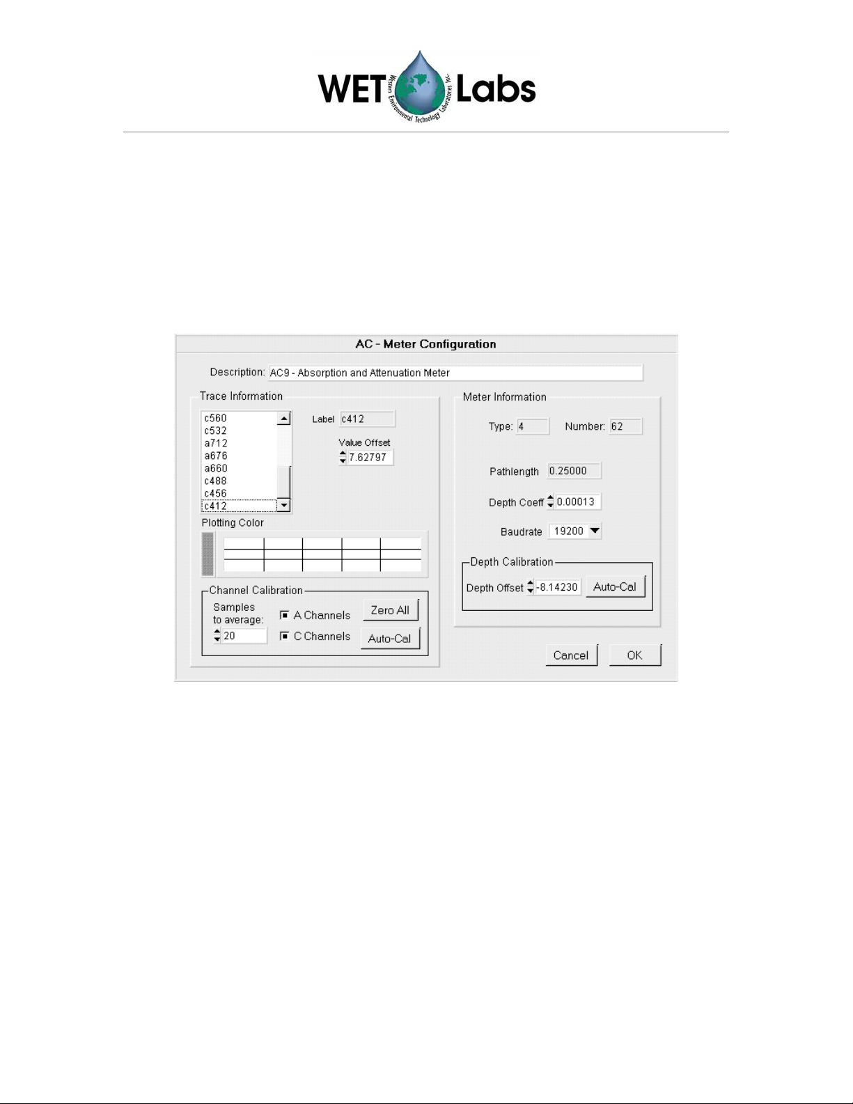
6.3.8 Changing a device's configuration (calibration)
To change an instrument’s calibration, a new device file must be collected. The
steps of this process are outlined below.
1. Making sure instrument is properly connected to a power supply and host
computer and that WETView is properly loaded and operational, start the
program and load an existing device file. Use the FILE menu selection and
then Open Device.
2. Open the Configure dialog box. Use the FILE menu selection and then
Configure.
WETView 5.0a User’s Guide (WETView) Revision E 12 April 2001 7
Page 10
3. In the lower left-hand corner you will see a sub-dialog box with control
buttons for Zero All and Auto Cal. It is the Auto Cal control that collects new
offsets for a device file. Note the option for number of samples to average.
Select the number of individual samples you wish to average by using this
control. The default is 10 samples.
4. Once you have selected the number of samples over which to average, you
then can engage the Auto Cal control. A temporary pop-up window will notify
you as the calibration takes place. After the operation is complete you may
exit the Configuration dialog box by pressing OK in the lower right hand
corner.
5. When you exit you will be prompted as to whether you want to save the new
offset values.
Caution
Unless you deliberately save a device file the offsets you have collected
will not be permanently stored.
You may write over an older device file if you choose, but the program
will ask you if you are sure you want to do this. Otherwise you may write
to a new file.
6. Before you can use the new values, reload the newly made device file
using Open Device.
8 WETView 5.0a User’s Guide (WETView)Revision E 12 April 2001
Page 11
7. Configuration
Configuration is specific to each type of device. The ac-9 and HiStar meters are discussed
below.
7.1 Configuring the ac-9
You can change the following settings for the ac-9 meter:
• calibration offsets for absorption measurements
• calibration offset for depth measurement
The ac-9 measures the absorption and attenuation of 9 different wavelengths of light.
Each of the measured quantities has a calibration offset added to it so that the
resulting number is the difference between a clean water measurement and the
measurement in the field. You can manually set the value of this offset for each
channel; however, determining the correct value to use is not trivial.
Usually, a “clean water calibration run” is performed. Chemically pure water is run
through the instrument and the values for absorption and attenuation are averaged
over a number of samples. These values are then used as the calibration offsets.
The “Auto-Cal” button in the “Channel Calibration” area of the dialog does the
collecting and averaging for you. You can set the number of samples to collect and
average over.
The “Zero All” button sets all of the calibration offsets to 0.0 so you can collect the
raw (uncorrected) values from the meter. Note that these values are always
temperature-compensated.
WETView 5.0a User’s Guide (WETView) Revision E 12 April 2001 9
Page 12

See Appendix B, “Calculations” for a complete description of how these numbers are
used.
Caution
We recommend you change only the instrument description and the color used
for plotting it. Changing the baud rate will most likely cause WETView to be
unable to communicate with the ac-9. Changing the calibration constants will
affect the accuracy of your results.
7.2 Configuring the HiStar
You can change the following settings for the HiStar Meter:
• calibration offsets for absorption/attenuation measurements
• calibration offset for depth measurement
• communication speed (only for RS-232 connections)
• the number of wavelengths measured
7.2.1 Selecting the graph to display
From the “Graph” menu, choose the graph you want to display.
WETView provides three types of graphs: a vertical X-Y graph of absorption
versus time, a horizontal strip chart of absorption versus time, and a graph of
absorption versus temperature. There are trade-offs to be considered when
choosing which display to use.
The X-Y graph accurately plots both time and absorption, whereas the strip chart
accurately plots absorption, but uses a constant time base. However, the strip
10 WETView 5.0a User’s Guide (WETView)Revision E 12 April 2001
Page 13

chart scrolls continuously as data is collected, so you can have detailed view of
the most recently received data, whereas the X-Y graph is static. When the data
runs off the graph, it is not visible until you stop data acquisition and rescale the
graph. In either case, all data acquired is logged to the data file.
The absorption versus temperature graph is used for temperature calibration. The
temperature reported is the temperature internal to the instrument, not the ambient
temperature. Also, since the temperature is reported once for each set of ten data
lines, all ten data lines will be plotted at the same temperature. We recommend
setting the collection bin size to a multiple of 10.
7.2.2 Changing the graph options
Select the “Graph | Options...” item to change the appearance of the currently
displayed graph. For X-Y graphs, you may set the X and Y ranges and the number
of divisions for each axis. For strip charts, you may set the Y range and the speed
that the chart scrolls.
7.2.3 Starting an acquisition run
Press the “F1 to Start” button to begin acquiring data from the currently opened
device. This item is highlighted only if you have a device open. The function key
F1 works as well. As data is acquired, the traces you have selected (via the
“Options | Channels/Binning” menu item) are graphed. Graphing the data points
uses memory and for long collection runs WETView may exhaust all available
memory (this is not true for the Strip Chart graph). If WETView runs out of
memory, it erases the graph and begins graphing from where it left off. All
collected data is, of course, saved in a file, whether or not it was erased from the
graph.
7.2.4 Ending an acquisition run
Once acquisition begins, a “F2 to Stop” button is displayed near the top of the
screen. Selecting that button with the mouse, or pressing the F2 key stops data
acquisition.
7.2.5 Changing the acquisition options
Select the “Options | Channels/Binning” item to select which traces to display and
to set the collection and display bin sizes.
7.2.6 Quitting WETView
Select “Quit” to quit the WETView program.
WETView 5.0a User’s Guide (WETView) Revision E 12 April 2001 11
Page 14

Appendix A—Absorption Coefficient Computation
The transmittance is computed by taking the ratio of the signal value to the reference
value,
E
sig
T =
r
The raw absorption coefficient, a
a
raw
where Z is the length of the column of water.
The behavior of the electronics circuitry is dependent on temperature. To account for this,
the absorption coefficient is corrected by adding a temperature compensation offset,
These offsets are determined for each specific unit in the laboratory by measuring the
meter’s behavior of over a range of temperatures. The values collected during the
temperature calibration run are averaged over two degree intervals. This produces a table
of temperature offsets for a wide range of temperatures. WETView uses that table and
linear interpolation to compute the temperature compensation offset,
wavelength at any given temperature. The temperature-compensated raw absorption,
then, is given by:
′
Finally, this value is calibrated to subtract out the characteristic absorption of clean water.
The calibration constant, C, is calculated in the laboratory using clean water
measurements and published values. The final absorption coefficient, a, for a
measurement in the field, then, is:
=
Each data file contains the calibration constant, C, and the table of temperature
compensation values used for each channel.
E
ref
ln
−=
aa ∆−=
′
Caa +
()
T
r
Z
Tnraw
, is then computed as,
raw
∆
, for each
Tn
∆
Tn.
12 WETView 5.0a User’s Guide (WETView)Revision E 12 April 2001
Page 15

Appendix B—ac-9 Meter
ac-9 Theory of Operation
The WET Labs’ ac-9 has a white light source that is directed through a filter that
allows a narrow band of wavelengths. The resultant colored light is directed through a
beam splitter.
One beam from the splitter is sent through a column of water to a detector at the other
end. The voltage from the detector is amplified and converted to a digital value. The
transmitted light's energy is measured and that value, called the signal, is sent to the
host computer.
The other beam from the splitter is sent directly to a different detector, where it is
amplified and converted, giving the reference value for the light source. This
reference value is sent to the host as well.
The device has several filters mounted on a rotating wheel. For each different filter,
both the signal and reference voltages are measured.
The signal values are sent approximately ten times per second. For each group of ten
signal readings, the reference values are averaged and sent approximately once per
second.
The reference value line also includes temperature and depth, if they are supported by
the instrument.
Temperature
Temperature is calculated from the instrument’s raw data by the following equation:
eTdTcTbTaT
rawrawrawraw
321 −−−
++++=
where:
T = temperature in degrees centigrade
Traw = number of counts sent by the device
a = 10.61831
b = 0.045113
c = -4891.32
d = 208130.2
e = 1171473
Depth
Depth is calculated from the instrument's raw depth data by scaling and offsetting
by the depth calibration numbers that are read from the device configuration file.
WETView 5.0a User’s Guide (WETView) Revision E 12 April 2001 13
Page 16

D = mDr + b
where:
D = depth in meters
= raw number of counts sent by the device
D
raw
m = multiplier determined in the laboratory for each depth sensor unit and is
unique to that unit; stored in the configuration file
b = offset determined by calibrating the device at sea level (this can easily be
done in the field); stored in the configuration file
ac-9 Configuration File
Configuration files (with file extension .DEV) give calibration and other information
specific to a particular unit. These files are tab-delimited text files and have the
following format:
Line 1 Device name.
Line 2 Serial number: the serial number of the device that was used to collect the
data.
Line 3 Version number of the following structure. This should be “2.”
Line 4 Reserved for future use.
Line 5 Calibrations for depth meter: there are two values, the first is an offset and
the second is a multiplier.
Line 6 RS-232 baud rate that the instrument uses
Line 7 Optical path length through water (in meters).
Line 8 Number of temperature compensation bins.
Line 9 Several values (the count is given in the preceding line); each value is the
average temperature of the temperature bin.
Line 10–27 Each line describes one channel of the instrument; the first three fields are:
label for identifying the channel
color for plotting
clean water calibration constant (offset)
The rest of the line contains temperature compensation values that
correspond to the temperature bins given in the previous line.
Line 28 Reserved for future use
Line 29 Extra capabilities mask. This is a list of capabilities that the meter may have
in addition to the standard product. Currently, only one such capability
exists: an external temperature sensor. If the first number on this line is non-
zero, the meter supports such a sensor.
ac-9 Data Files
WETView saves data files in tab-delimited format. The file format of WETView files
is described below.
14 WETView 5.0a User’s Guide (WETView)Revision E 12 April 2001
Page 17

Line 1: Header line. Identifies the version of the program that created the file, and the
time and date of creation.
Lines 2–30: Exactly the same format as the configuration file. These lines contain the
calibration information that was used while collecting the data.
Line 31: Collection bin size. The number of samples that were averaged into each bin
during collection.
Data lines
The rest of the file contains lines of data values. Each line of data starts with a
zero-based time stamp. Times are given in milliseconds. The rest of the fields on
the line are the data from the device. The data is given as absorption values, after
referencing, calibration and temperature correction.
Reference lines
A reference line is a data line that has some extra information appended to it.
1. The first number after the data values is the temperature (deg C).
2. The second number is the sample rate (samples per second).
3. The third number is the depth (in meters, if the meter supports depth).
4. The fourth number is the external temperature, if the meter supports it.
5. The rest of the line contains channel reference values.
A full data line with references then looks like:
Time Chan
Chan2 ... Chann Temp Rate Depth ExtTemp Ref1 Ref2 ... Refn
1
The reference values are raw values; no scaling or calibration is applied to them.
These are the values that are used in computing the data values for the following
set of data lines.
There is a possible ambiguity when the collection bin size is greater than one.
Since a bin contains multiple samples, some of the samples in a bin may be
computed with one set of reference values and others computed with a different
set. The ac-9 uses one set of references for every ten samples. If the collection bin
size is six, the first bin (six samples) uses the same reference values, but the
second bin uses one set of references for the first four samples and a different set
for the last two samples. This makes deconvoluting to the raw data rather
complicated.
If you need to deconvolute to raw data, choose a bin size of 1, 2, 5, 10 or an
integer multiple of ten. This ensures that the reference values given for a bin
apply to all samples in that bin.
Example
For example, given the configuration file:
ac9 Absorption and Attenuation Meter
04000103 ; serial number
2 ; structure version number
WETView 5.0a User’s Guide (WETView) Revision E 12 April 2001 15
Page 18

Reserved ; reserved for future
5.41000 0.27000 ; depth calibration
19200 ; baud rate
0.10 ; pathlength = 10 cm
a650 Blue 1.20000 23.00000 2.43000
a560 Green 1.13000 23.00000 2.45000
a532 Brown 1.24000 23.00000 2.65000
c712 Red 1.08000 23.00000 2.31000
c676 Magenta 1.41000 23.00000 2.74000
c660 Gray 1.55000 23.00000 2.56000
a488 LtBlue 1.16000 23.00000 2.44000
a456 LtGreen 1.19000 23.00000 2.52000
a412 Yellow 1.33000 23.00000 2.54000
c650 Blue 0.98000 23.00000 2.47000
c560 Green 1.58000 23.00000 2.36000
c532 Brown 1.94000 23.00000 2.51000
a712 Red 1.32000 23.00000 2.57000
a676 Magenta 1.74000 23.00000 2.46000
a660 Gray 1.83000 23.00000 2.49000
c488 LtBlue 1.35000 23.00000 2.38000
c456 LtGreen 1.50000 23.00000 2.33000
c412 Yellow 1.11000 23.00000 2.39000
0.0035 0.004 0.015 0.02 0.015 0.02 2500 2000 1000 0.01 0.01 …
0 ; auxiliary capabilities
The data file for an ac-9 begins as:
WetView ver 5.0 06/22/93 08:17:44
ac9 Absorption and Attenuation Meter
04000103 ; serial number
2 ; structure version number
Reserved ; reserved for future
5.41000 0.27000 ; depth calibration
19200 ; baud rate
0.10 ; pathlength = 10 cm
a650 Blue 1.20000 23.00000 2.43000
a560 Green 1.13000 23.00000 2.45000
a532 Brown 1.24000 23.00000 2.65000
c712 Red 1.08000 23.00000 2.31000
c676 Magenta 1.41000 23.00000 2.74000
c660 Gray 1.55000 23.00000 2.56000
a488 LtBlue 1.16000 23.00000 2.44000
a456 LtGreen 1.19000 23.00000 2.52000
a412 Yellow 1.33000 23.00000 2.54000
c650 Blue 0.98000 23.00000 2.47000
c560 Green 1.58000 23.00000 2.36000
c532 Brown 1.94000 23.00000 2.51000
a712 Red 1.32000 23.00000 2.57000
a676 Magenta 1.74000 23.00000 2.46000
a660 Gray 1.83000 23.00000 2.49000
c488 LtBlue 1.35000 23.00000 2.38000
c456 LtGreen 1.50000 23.00000 2.33000
c412 Yellow 1.11000 23.00000 2.39000
0.0035 0.004 0.015 0.02 0.015 0.02 2500 2000 1000 0.01 0.01 …
0 ; auxiliary capabilities
1 ; acquisition binsize
0 1.53275 1.13881 1.31256 0.51315 1.41231 2.51512 ...
160 1.53070 1.13055 1.31583 0.51229 1.41614 2.51415 ...
330 1.53627 1.13536 1.31511 0.51467 1.41151 2.51614 ...
(etc)
The fields for the reference line for the ac-9 are:
field # contents
1 time in milliseconds
2 absorption for 650 nm
16 WETView 5.0a User’s Guide (WETView)Revision E 12 April 2001
Page 19

3 absorption for 560 nm
4 absorption for 532 nm
5 attenuation for 712 nm
6 attenuation for 676 nm
7 attenuation for 660 nm
8 absorption for 488 nm
9 absorption for 456 nm
10 absorption for 412 nm
11 attenuation for 650 nm
12 attenuation for 560 nm
13 attenuation for 532 nm
14 absorption for 712 nm
15 absorption for 676 nm
16 absorption for 660 nm
17 attenuation for 488 nm
18 attenuation for 456 nm
19 attenuation for 412 nm
20 temperature (
21 sample rate (samples per second)
22 depth (meters)
23 reserved
24 reference for a650
25 reference for a560
26 reference for a532
27 reference for c712
28 reference for c676
29 reference for c660
30 reference for a488
31 reference for a456
32 reference for a412
33 reference for c650
34 reference for c560
35 reference for c532
36 reference for a712
37 reference for a676
38 reference for a660
39 reference for c488
40 reference for c456
41 reference for c412
o
C)
The information in a data line is exactly the same as the first 19 fields of the
reference line.
ac-9 Complete Example
This section gives a complete example of an ac-9 device configuration file, a raw data
record, and the computed results written to a data file.
Configuration file
Below is the configuration file for the ac9 meter used in this example.
ac-9 Absorption and Attenuation Meter
00000121 ; serial number
2 ; structure version number
Reserved ; reserved for future
5.3 0.3 ; depth calibration
19200 ; baud rate
WETView 5.0a User’s Guide (WETView) Revision E 12 April 2001 17
Page 20

0.25 ; path length (meters)
15 ; number of temperature bins
5.5233 8.4553 11.4712 … ; temperature bins
a610 Blue 7.6242 0.1411 0.1028 0.0389 …
a620 Green 7.6819 0.1403 0.1041 0.0393 …
a630 Brown 7.6963 0.1369 0.1034 0.0409 …
c610 Red 6.8377 0.1351 0.1045 0.0427 …
c620 Magenta 6.9157 0.1299 0.1034 0.0423 …
c630 Black 7.0137 0.1203 0.0987 0.0423 …
a640 LtBlue 7.1391 0.1169 0.0980 0.0427 …
a650 LtGreen 7.2244 0.1115 0.0959 0.0436 …
a660 Yellow 7.2360 0.1029 0.0893 0.0411 …
c640 Blue 7.1407 0.1001 0.0901 0.0435 …
c650 Green 6.8605 0.0979 0.0861 0.0429 …
c660 Brown 7.2408 0.0949 0.0851 0.0428 …
a670 Red 7.3416 0.0935 0.0839 0.0417 …
a680 Magenta 7.3578 0.0924 0.0827 0.0431 …
a690 Black 7.3922 0.0911 0.0824 0.0436 …
c670 LtBlue 6.0476 0.0903 0.0815 0.0442 …
c680 LtGreen 6.4225 0.0903 0.0805 0.0431 …
c690 Yellow 6.5098 0.0876 0.0793 0.0405 …
0.0035 0.004 0.015 0.02 … ; reserved info
0 ; auxiliary capabilities
Raw data
Below is one record of raw data that was captured from the device. It has been
converted to hexadecimal, formatted and commented. Note that the two-byte and
four-byte values are byte-reversed. That is, the bytes within a word are read from
right to left. This reflects the way the Intel 386 and 486 processors store values in
memory.
18 WETView 5.0a User’s Guide (WETView)Revision E 12 April 2001
Page 21

00FF00FF registration word
7A02 record length, from this word
21010000 serial number
0000 status
DB13 sample rate
1600 depth
34FF external temperature
6410 171E 89 2D20 0F 0319 1B …
7510 171E CB 2C20 EE 0119 A3 …
8510 161E 84 2E20 0A 0119 F2 …
9510 131E F1 2920 DE FE18 DF …
A510 151E 9B 2B20 BC 0119 51 …
B510 151E 7A 2B20 BA 0119 9A …
C510 161E 5D 2C20 99 0019 49 …
D510 141E F5 2B20 85 0019 B1 …
E510 121E 3F 2820 76 FF18 11 …
F610 141E 05 2A20 5E 0019 35 …
7804 C8 B604 C0 A603 66 … 3 references and temperature
9701 temperature
65D00000 checksum (FF00FF00 through refs)
00000000 padding (4 null bytes)
Registration
word
Record length
Serial number = 00000121
Status = 0000 Zero indicates normal operation.
Sample rate = 14F9 hex = 5083
Depth = 0016 hex = 22
External Temp = 34FF hex
For the purpose of this discussion, we skip to the third-from-last line of the data
record. This is the reference line, and values here will be used in the computation
of the absorption values for each channel.
through checksum
first sample, time and data
second sample, time and data
o
o
o
tenth sample, time and data
= 00FF00FF hex
= 7A02 hex = 634 bytes
This is the thirty-third ac-9 meter produced. Production numbers
begin with 0100 hex.
This is a count of the time used to take one sample. It is scaled by
0.0000316 to match the hardware’s clock rate, then inverted to give
samples per second:
1 / (5083 * 0.0000316) = 6.226
This reflects the voltage read from the depth sensor. It is scaled and
offset by the values from the configuration file.
22 * 0.3 + 5.3 = 11.9 meters
This word is ignored for this meter because the meter does not have
an external temperature probe in it. This is determined by the last line
of the configuration file: the value is zero.
WETView 5.0a User’s Guide (WETView) Revision E 12 April 2001 19
Page 22

Reference a610
Temperature = 0F01 hex = 271
Absorption 610 = 171E 89 hex = 8986135
= 7804 C8 hex = 13108344
This is the reference value for the first channel (ab610). This is a 24bit value indicating the output from an analog to digital converter.
This represents a fraction of the input voltage. To convert from counts
to this fraction, the value is divided by 2
13108344/16777216 = 0.7813
The temperature is given as a reading from a thermistor. The
manufacturer of the thermistor provides a table correlating the reading
(counts) to temperature. That table fits the polynomial equation given
above. Using 407 counts, we get: 10.61831
+ 0.045113 * 271
+ -4891.32 * 1/271
+ 208130.2 * 1/271
+ 1171473 * 1/2713 = 7.69 degrees C
This is the signal value for the first channel (a610). This 24-bit value
is converted to raw voltage in the same manner as for reference
values.
24
(16777216).
2
8986135 / 16777216 = 0.5356 VDC
Raw absorption is computed from the signal and reference values as
described above:
−=ln
a
raw
E
ref
Z
E
sig
The device’s optical path length is read from the configuration file.
0.5356
ln
−
0.7813
=
a
raw
=
25.0
1-
meter 1.5103
The temperature correction is then applied using the temperature from
the reference line and the channel’s correction table from the
configuration file. The approximate correction value is linearly
interpolated from the table. First, the correct temperature bin is
determined by finding the two bin temperatures, T
the current temperature. Then, using the values,
and T1, that bracket
0
∆
Tn
and
∆
Tn+1
, from the
table,
()
−
TT
0
+∆=∆
()
−
()
*
TT
01
∆−∆
+1
TnTnTnT
where,
∆
=compensation constant
T
20 WETView 5.0a User’s Guide (WETView)Revision E 12 April 2001
Page 23

T=current temperature, 7.69
T
=first bin temperature, 5.5233
0
T
=second bin temperature, 8.4553
1
∆
=first value, 0.1411
Tn
∆
=second value, 0.1028
Tn+1
Using these values,
1411.0
T
0.1127m
=
Subtracting this from the raw absorption,
()
+=∆
()
1-
5233.569.7
−
5233.54553.8
−
()
1411.01028.0*
−
′
=
Finally, adding in the calibration offset for a610,
Checksum = 65D00000 = 53349
The checksum is the sum of all the bytes of the record, beginning
with the registration word and ending with the temperature. For this
record, the checksum is 53349. This is used to verify that the record
was received correctly by WETView.
Padding
= 00000000
These four null bytes separate records. They are ignored. The
advantage of having them is that if a character is lost in transmission,
WETView will read one byte past the end of the corrupted record. If
there were no padding bytes, the first byte of the next record would
have been read, corrupting that record as well. With the padding
bytes, however, if a character is lost in transmission, then WETView
will read one byte past the end of the record, which will be a padding
byte, and it can be safely discarded. The next record will be read
correctly.
aa
∆−=
Traw
0.1127 1.5103
−=
1.3976
′
+
=
=
Caa
+=
7.62423976.1
9.0218
WETView 5.0a User’s Guide (WETView) Revision E 12 April 2001 21
Page 24

Appendix C—HiStar Meter
Theory of Operation
HiStar uses fiber optics and small spectrometers to provide a multi-spectral view of
marine optical parameters. Two white tungsten lamps provide the source light for the
absorption, attenuation and reference paths. Using bundles of fibers with different
packing characteristics, the source light uses a color correction filter and a mixing rod
to improve the linearity of the output signal and reference spectrum.
The “a” transmitter is a specially designed termination that provides an isotropic
source of light. The “c” transmitter is fed by a separate fiber optic bundle, and uses an
achromatic lens to supply a collimated beam of light. Both beams then pass through
quartz pressure windows and enter the 250 mm flow cell.
In the “c” side of the flow cell, scattered light that intersects the side wall of the cell is
absorbed and “lost” to the system. The “a” tube of the flow cell is lined with an
aluminized reflective quartz tube so that light scattered forward of the critical angle
(approximately 41 degrees) is reflected back into the path and collected by the
detector. Only absorbed light—and the small amount of light scattered backwards—is
“lost” to the system. Thus the “c” side measures the attenuation of light due to both
scattering and absorption while the “a” side measures absorption only. After applying
several corrections to the “a” measurement, the corrected “a” value can be subtracted
from the beam transmission, “c” to get a good estimate of “b,” the attenuation due to
scattering.
After transiting either the “a” or the “c” flow tube, the remaining light passes through
another quartz window and enters the receiver optics. An achromatic lens on the “c”
side focuses the beam onto the end of a fiber optic bundle. This bundle is coupled
through a chopper to a spectrometer that in turn is connected to the instrument
electronics.
Each spectrometer also measures reference. This path is primarily to provide a
method of accounting for tiny variations in the source light due to lamp aging, voltage
fluctuations and/or temperature variations.
Computations
Instrument Internal Temperature
Temperature is calculated from the instrument's raw data by the following
equation:
eTdTcTbTaT
rawrawrawraw
321 −−−
++++=
where:
22 WETView 5.0a User’s Guide (WETView)Revision E 12 April 2001
Page 25
T = temperature in degrees centigrade
Traw = number of counts sent by the device
a = 10.61831
b = 0.045113
c = -4891.32
d = 208130.2
e = 1171473
Depth (Optional Sensor)
Depth is calculated from the instrument’s raw depth data by scaling and offsetting
the depth calibration numbers which are read from the device configuration file.
D = mD
raw
+ b
where:
D = depth in meters
D
= raw number of counts sent by the device
raw
m = multiplier determined in the laboratory for each depth sensor
unit and is unique to that unit; stored in the configuration file
b = offset determined by calibrating the device at sea level (this can
easily be done in the field); stored in the configuration file
HiStar Configuration File
HiStar configuration files (with file extension .DEV) give calibration and other
information specific to a particular unit. These files are tab-delimited text files and
have the following format:
Line 1 Device name.
Line 2 Serial number. The serial number of the device that was used to collect
the data.
Line 3 Version number of the following structure. This should be “2.”
Line 4 Reserved for future use.
Line 5 Calibrations for depth meter: there are two values, the first is an offset
and the second is a multiplier.
Line 6 RS-232 baud rate that the instrument uses
Line 7 Optical path length through water (in meters).
Line 8 Line 8 Number of pixels to skip in acquisition. The meter can measure
up to 100 wavelengths (pixels). A skip value of 1 means that all 100
wavelengths are measured. A skip value of 2 means that every other
wavelength is measured. Skip value may be 1, 2, 3, or 4.
Line 9 Number of temperature compensation bins.
Line 10 Several values (the count is given in the preceding line); each value is the
average temperature of the temperature bin.
WETView 5.0a User’s Guide (WETView) Revision E 12 April 2001 23
Page 26

Lines
11–110
Each line describes one wavelength of the instrument; the first four
fields are:
label for identifying the wavelength
color for plotting
clean water calibration constant for attenuation, c
clean water calibration constant for absorption, a
The rest of the line contains temperature compensation values that
correspond to the temperature bins given in the previous line. The first
n values are for c, the next n values are for a, where n is the number of
temperature bins.
Line 111 Reserved for future use.
For example:
HiStar Meter - skipPixel = 1
F1000007 ; serial number
2 ; structure version number
Reserved
-363.6 1 ; Depth calibration
38400 ; Baud rate
0.25 ; Path length (meters)
1 ; skip value
; number of temperature
26
4.904444 5.470667 6.48225 7.474054 8.520571 …
a406.4 LtMagenta -3.979 1.271513 -0.10979 -0.10665 -0.10019 -0.09359 -0.08665 …
a409.7 1 -3.95405 1.286457 -0.10216 -0.09913 -0.09334 -0.08673 -0.0809 …
a413 2 -3.91322 1.309278 -0.098 -0.09532 -0.09041 -0.08499 -0.07932 …
a416.3 3 -3.8625 1.338559 -0.09317 -0.09196 -0.08846 -0.0832 -0.0765 …
a419.6 5 -3.8105 1.366215 -0.0909 -0.08865 -0.08503 -0.07958 -0.07433 …
a423 6 -3.74401 1.38832 -0.08808 -0.08438 -0.08033 -0.07801 -0.07311 …
a426.3 7 -3.66619 1.415876 -0.08195 -0.08141 -0.07761 -0.07336 -0.06921 …
bins
o
o
o
a716.4 117 2.790931 2.100402 -0.08213 -0.07874 -0.0755 -0.0728 -0.06955 …
a719.7 119 2.749065 1.91727 -0.08037 -0.07621 -0.07138 -0.07033 -0.07255 …
a722.9 120 2.670427 1.687524 -0.08962 -0.08543 -0.08108 -0.07562 -0.06954 …
a726.2 121 2.540299 1.423893 -0.08774 -0.08437 -0.07957 -0.07683 -0.07019 …
a729.5 DkGray 2.356431 1.179627 -0.08659 -0.0844 -0.07951 -0.07743 -0.07197 …
a732.7 LtRed 2.203966 1.026263 -0.0733 -0.07195 -0.06881 -0.06545 -0.0611 …
0 0 0 0 0 0 0 0 0 0 …
24 WETView 5.0a User’s Guide (WETView)Revision E 12 April 2001
Page 27

HiStar Data Files
WETView saves data files in tab-delimited format. The file format for data files is as
follows:
Line 1 Header line. Identifies the version of the program that created the file,
and the time and date of creation.
Line 2–11 Exactly the same format as the configuration file. These lines contain
the calibration information that was used while collecting the data.
Lines 12–111 Collection bin size. This is the number of samples that were averaged
into each bin during collection.
Line 112 Reserved for future use
Line 113 Acquisition bin size
Line 114 WETView label
Lines 115–n Data lines. Each line starts with a zero-based time stamp. Times are in
milliseconds from the time the instrument is turned on. Data is given as
final values, after referencing, calibration and temperature correction.
The first group of values is the “c” values, followed by the “a” values.
After the data, there are four additional columns:
1. instrument temperature (deg C)
2. not used (0)
3. depth (in meters, if the HiStar is equipped with a depth sensor)
4. reserved for future use.
A data line then looks like:
Time c(λ
), c(λ2),… c(λn), a(λ1), a(λ2), … a(λn) Temp, 0.0, Depth, 0.0
1
WETView 5.0a User’s Guide (WETView) Revision E 12 April 2001 25
Page 28

An example of a data file:
WetView
ver 6.0A 5/11/00 9:26:13
HiStar Meter - skipPixel = 1
F100000E ; serial number
2 ; structure version number
Reserved
-363.6 1 ; Depth calibration
38400 ; Baud rate
0.25 ; Path length (meters)
1 ; skip value
0 ; number of temperature bins
0 ; temperature bins
a406.4 LtMagenta -1.32085 3.010416
a409.7 1 -1.41032 3.034271
a413 2 -1.47975 3.047789
a416.3 3 -1.53713 3.071629
a419.6 5 -1.57037 3.088684
a423 6 -1.59529 3.114031
a426.3 7 -1.58554 3.146257
a429.6 8 -1.56934 3.147711
a432.9 10 -1.54645 3.14934
a436.2 11 -1.51666 3.162758
o
o
o
a732.7 LtRed 5.444705 5.247366
0 0 0 0 0 0 0 0 0
2 ; acquisition binsize
c406.4 c409.7 c413 c416.3 c419.6 c423 c426.3 c429.6
1560 0.00083 -0.00196 -0.00328 0.00008 -0.00065 0.00325 0.00232 -0.00165 …
4710 -0.00199 -0.00324 0.0017 0.00008 -0.00065 0.00075 0.00048 0.0008 …
7860 0.00122 -0.00047 -0.00105 -0.00024 -0.00149 -0.00001 0.00299 0.00019 …
HiStar Calculations
The manufacturer of the thermistor provides a table correlating the reading
(resistance) to temperature. That table fits the polynomial equation:
T
=
1
()
++
RcRba
lnln(
−
3
16.273
where:
a = 0.00093135
b = 0.000221631
c = 0.000000125741
R is the resistance of the thermistor:
26 WETView 5.0a User’s Guide (WETView)Revision E 12 April 2001
Page 29

R−=
V
000,10*
V
5.2
where:
V is the voltage read from the A/D converters:
part
part
2
1
V =
*27.1
where:
part
and part2 are raw data sent by the meter. (Refer to the raw data record in
1
the next section.)
HiStar Complete Example
This section gives a complete example of a HiStar device configuration file, a raw
data record, and the computed results written to a data file.
Configuration file
Below is the configuration file for the HiStar meter used in this example.
HiStar Meter
F1000004 ; serial number
2 ; structure version number
Reserved ; reserved for future
5.3 0.3 ; depth calibration
57600 ; baud rate
0.25 ; path length (meters)
1 ; skip value
7 ; number of temperature bins
7.2655 12.2142 17.4269 22.4909… ; temperature bins
w406.4 0 -1.7154 -1.1570 0.1457 0.1038 0.0392 0.0101 …
w409.7 1 -1.6953 -1.1241 0.1411 0.1028 0.0389 0.0112 …
w413.0 2 -1.6779 -1.1429 0.1403 0.1041 0.0409 0.0113 …
w416.3 3 -1.6619 -1.0984 0.1369 0.1034 0.0427 0.0129 …
w419.6 4 -1.6395 -1.0910 0.1351 0.1045 0.0423 0.0119 …
w423.0 5 -1.6217 -1.1006 0.1299 0.1034 0.0423 0.0126 …
o
o
o
w726.2 121 -2.1861 -3.9821 0.0486 0.0442 0.0313 0.0182 …
w729.5 122 -2.2104 -4.0484 0.0487 0.0440 0.0319 0.0198 …
w732.7 123 -2.2311 -4.1049 0.0503 0.0455 0.0341 0.0216 …
0.0000 0.0000 0.0000 0.0000 0.0000 0.0000 0.0000 0.0000 …
Raw data
Below is one record of raw data that was captured from the device. It has been
converted to hexadecimal, formatted and commented. Note that the two-byte and
four-byte values are byte-reversed. That is, the bytes within a word are read from
right to left. This reflects the way the Intel 386 and 486 processors store values in
memory.
FF00FF00
0278 record length, from this word
WETView 5.0a User’s Guide (WETView) Revision E 12 April 2001 27
registration word
through checksum
Page 30

01 packet type; reserved for future use
01 pixel skip value
F1000001 serial number
0001 status
0000 reserved for future use
000A depth
243E temperature, part 1
3703 temperature, part 2
7FFF0000 reserved for future use
0006DB8C time
1D start pixel (used internally only)
64 pixel count (used internally only)
0886 02A4 04D1 2BA0 c reference, a reference, c signal, a signal
094E 02CE 0526 2BA9 c reference, a reference, c signal, a signal
o o
o o
o o
2394 0BE0 1642 2BCC
233C 0BD6 162A 2BC4
22FE 0BC7 1618 2BR9 c reference, a reference, c signal, a signal for last wavelength
AF2B checksum
28 WETView 5.0a User’s Guide (WETView)Revision E 12 April 2001
Page 31

Registration
word
Record length = 0278 hex = 634 bytes
Serial number = F1000008
Packet type = 01
Pixel skip
value
Status = 0001
Reserved <2 undefined bytes>
Depth = 000A hex = 10
= FF00FF00 hex
This is the eighth HiStar meter produced (production numbers begin with 0000
hex).
Reserved for future use.
= 01
This value can be 1, 2, 3, or 4. There are 100 wavelengths at most. The meter can
be configured to read every wavelength, every other, every third, or every fourth
wavelength. This results in 100, 50, 33, or 25 value reported. This field tells how
the meter is configured. In this example, it is set to read out all 100 wavelengths.
Reserved for future use.
Reserved for future use.
This reflects the voltage read from the depth sensor. It is scaled and offset by the
values from the configuration file.
Temperature,
part 1
Temperature,
part 2
10 * 0.3 + 5.3 = 8.3 meters
= 243E hex = 9278
= 3703 hex = 14083
Using the equation given above, we get:
14083
=V
=
and,
=R
=
and finally,
=
T
=
*27.1
9278
92772.1
000,10*92772.1
92772.15.2
−
1.33685
1
()
++
cba
C degrees 325.22
−
3
1.33685ln1.33685ln
16.273
WETView 5.0a User’s Guide (WETView) Revision E 12 April 2001 29
Page 32

Reserved <4 undefined bytes>
Reserved for future use.
Data,
wavelength 1
= 0886 02A4 04D1 hex = 2182 676 1233
This is the data read for the first wavelength: reference, c, and a channels,
respectively. Raw absorption is computed from the signal and reference values as
described above:
−=ln
a
raw
E
ref
Z
E
sig
The channel's calibration constant and the device's optical path length are read
from the configuration file.
1233
2182
25.0
1-
meter 2.2832
−
ln
=
a
raw
=
and,
676
2182
25.0
1-
meter 4.6872
−
ln
=
c
raw
=
The temperature correction is then applied using the temperature from the
reference line and the channel's correction table from the configuration file. The
approximate correction value is linearly interpolated from the table. First, the
and
0
correct temperature bin is determined by finding the two bin temperatures, T
and T1, that bracket the current temperature. Then, using the values,
∆
, from the table,
Tn+1
vK
0
T
+=
()
TT
−
0
()
* vv
−
()
TT
−
01
01
∆
Tn
where,
∆
= compensation constant
T
T = current temperature, 22.325
= first bin temperature, 17.4269
T
0
T
= second bin temperature, 22.4909
1
∆
= first value, 0.0392
Tn
∆
= second value, 0.0101
Tn+1
Using these values,
30 WETView 5.0a User’s Guide (WETView)Revision E 12 April 2001
Page 33

0.0392
T
=
Subtracting this from the raw absorption,
′
aa
2.2722
=
Finally, adding in the calibration offset for a610,
′
+
= Caa
0.5568
=
Checksum = AF2B = 44843
The checksum is the sum of all the bytes of the record, beginning with the
registration word and ending with the byte just before this checksum. For this
record, the checksum is 44843. This is used to verify that the record was received
correctly by WETView.
()
+=∆
()
1-
m 0.0110
∆−=
Traw
0.01102832.2
−=
−+=
4269.17325.22
−
4269.174909.22
−
)7154.1(2722.2
()
0.03920101.0*
−
WETView 5.0a User’s Guide (WETView) Revision E 12 April 2001 31
Page 34

Page 35
WETView 5.0a
User’s Guide
WET Labs, Inc.
P.O. Box 518
Philomath, OR 97370
Tel: 541-929-5650
fax: 541-929-5277
http://www.wetlabs.com
Revision Date Revision Description Originator
A 02/08/00 Begin revision control H. Van Zee
B 04/12/00 Correct calibration offset for ac-9 (DCR 20) C. de Lespinasse
C 05/23/00 Correct data and device files for HiStar (DCR 31) D. Hankins, H. Van Zee
D 07/12/00 Correct equation on temperature correction
E 4/12/01 Delete references to three-spectrometer HiStar
Revision History
C. de Lespinasse
algorithm (DCR 47)
D. Hankins
(DCR 102)
WETView 5.0a User’s Guide (WETView) Revision E 12 April 2001
 Loading...