Wet Labs acprot User Manual

ac Meter

Protocol Document

WET Labs, Inc.
P.O. Box 518
Philomath, OR 97370
541 929-5650
fax: [phone]
www.wetlabs.com

Table of Contents

Acknowledgements ............................................................................ 1

1.

Introduction ............................................................................... 1

2.

Background and Evolution ........................................................ 3

2.1 ac-9 ................................................................................................................. 3

2.1.1 Interference Filters ...........................................................................................3

2.1.2 Absorption Detector .........................................................................................3

2.1.3 Internal Optics ..................................................................................................3

2.1.4 Windows ..........................................................................................................3

2.1.5 Flow Tubes.......................................................................................................3

2.1.6 Improved Referencing .....................................................................................3

2.1.7 Electronics........................................................................................................3

2.1.8 Mechanical .......................................................................................................3

2.2 ac-s .................................................................................................................... 4

3.

Operation .................................................................................. 5

3.1 Orientation ...................................................................................................... 5

3.2 Testing ............................................................................................................ 6

3.3 Mounting ......................................................................................................... 8

3.4 Plumbing and Tubing ...................................................................................... 9

3.5 Attaching Prefilter to Remove the Particulate Fraction .................................. 10

3.6 Deployment .................................................................................................. 10

3.6.1 Moorings ........................................................................................................10

3.6.2 Towed Bodies ................................................................................................12

Ship Underway and General Benchtop Operation ......................................................13

3.6.4 Profiling .........................................................................................................13

4.

Calibration ............................................................................. 15

4.1 WET Labs Calibration Procedures ................................................................ 15

4.1.1 Factory Pre-calibration Procedures ................................................................15

4.1.2 Factory Temperature Calibration ...................................................................15

4.1.3 Factory Water Calibration..............................................................................16

4.1.4 Factory Air Calibration ..................................................................................17

4.2 Air Tracking Procedures ............................................................................... 18

4.2.1 When to Use Air Tracking ............................................................................18

4.2.2 Air Tracking Protocol ...................................................................................19

4.3 Field Water Calibration Procedures .............................................................. 20

4.3.1 When to use Field Water Calibrations ...........................................................20

ac meter Protocol (acprot) Revision N 21 May 2008 i

4.3.2 Field Clean Water Production System ...........................................................20

4.3.3 Field Water Calibration Protocol ...................................................................22

5.

Data Processing ..................................................................... 26

5.1 Basic WETVIEW Calculations ...................................................................... 26

5.2 Merging ........................................................................................................ 27

5.3 Time Lag Correction ..................................................................................... 27

5.4 Water Temperature and Salinity Corrections ................................................ 28

5.6 Reflective Tube Scattering Correction .......................................................... 30

5.7 Attenuation Acceptance Angle Correction ..................................................... 31

5.8 Other Processing Notes ................................................................................. 32

5.8.1 Considering Spatial Variability......................................................................32

5.8.2 ac-s Mid-spectrum Discontinuities ................................................................32

5.8.3 Outliers ...........................................................................................................32

5.9 Directly Derived Products ............................................................................. 32

5.9.1 Computing Total Absorption and Attenuation from Measurements .............32

5.10 Reality Checks ............................................................................................... 39

6.

References ............................................................................. 41

Appendix 1. Device Files ................................................................. 42

Appendix 2. Sample Matlab Routines: ............................................. 46

ii ac meter Protocol (acprot) Revision N 21 May 2008

ac meter Protocol (acprot) Revision N 21 May 2008 iii

Acknowledgements

While virtually everyone who has sought meaningful and consistent results has contributed to
this evolution of the ac-9 protocol, several scientists provided pioneering efforts, and direct input
on this document. They include Scott Pegau, Percy Donaghay, Mike Twardowski, Scott
Freeman, and Alan Weidemann.

1. Introduction

The ac-9 was originally developed under Naval Research Laboratory sponsorship. Primary
development occurred over a 6-month time span culminating in delivery in September 1993.
Since initial delivery, approximately 180 more units have been used in applications ranging from
tow-yos to long-term moorings. In 2004 a follow-on hyperspectral absorption and attenuation
device, the ac-s, was also introduced. While the manuals for these devices cover basic operation
and processing of the raw signals into engineering units, certain protocols for usage and data
processing have been developed over the years, largely by the scientific community, to provide
the highest possible accuracy in absorption and attenuation data and directly derived products.
As a supplement to the ac-9 and ac-s user manuals, this document details these protocols.

Protocols for ac-9 and ac-s use are broken down into three primary sections. We first discuss
basic operation and deployment issues. Second, we discuss the ac-9 laboratory and field
calibration. Third, we delineate the steps for processing and correction of the data obtained by
the instrument. These three sections are prefaced by an overview of the various engineering
improvements that have occurred over the past few years. A final section provides a concise
summary of the data processing steps as well as a reality check table for determination of data
quality.

This protocol is intended as a hands-on guide for data collection and processing of data from the
ac-9 and/or ac-s. For more general discussions of meter applications or measurement theory you
may wish to consult the references contained in the back of the document.

One should remember that ac-9 and ac-s usage and data processing techniques are subject to
continual evolution. This document attempts to summarize the state of the art in commonly
applied techniques as they stand today. Even as the document is being written, researchers
continue to explore and refine new possibilities in applications, calibration, and processing.
Similarly, engineers at WET Labs continue to strive to improve instrument capabilities,
reliability and ease of use. We urge researchers to stay in touch through our web site
(http://www.wetlabs.com) or by calling us. Likewise, if you have any suggestions or additions to
this protocol document please let us know.

ac meter Protocol (acprot) Revision N 21 May 2008 1
2 ac meter Protocol (acprot) Revision N 21 May 2008

2. Background and Evolution

2.1 ac-9

The ac-9 has gone through several major design modifications in the last several years to
improve the overall stability and reliability of the instrument. Described below are some of the
more significant changes that have been successfully implemented.

2.1.1 Interference Filters

The ac-9 uses nine band-pass filters to spectrally discriminate the light from a tungsten lamp.
These nine filters are mounted on a filter wheel located in the transmitter pressure housing.

2.1.2 Absorption Detector

The absorption detectors have gone through numerous modifications in effort to improve
long-term reliability, stability, and ease of manufacture.

2.1.3 Internal Optics

Optical mounts for all the lenses and filters were improved to provide better stability and
easier meter assembly.

2.1.4 Windows

Pressure window apertures were increased to eliminate possible partial beam occlusions.

2.1.5 Flow Tubes

The flow tubes and sleeves went through several stages of modifications. Most recently inlet
and outlet nozzle diameters have been increased to provide improved flushing.

2.1.6 Improved Referencing

The ac-9 employs a reference detector within the transmitter optics. This detector measures
the output energy from the source that in turn provides a normalized output from the meter.
With the original filters and optics, throughput in the blue region of the spectrum was not
sufficient to allow one-to-one referencing. We thus integrated values of all three blue
wavelengths and used the single value as a reference for the blue wavelengths. With the
increased throughput provided by the new filters, we have returned to a one-to-one
referencing scheme throughout the spectrum.

2.1.7 Electronics

In 1995 new electronics were developed for the meter. The new board set allowed more
efficient manufacturing and characterization, more flexibility in interfacing, and improved
resistance to shock and vibration.

2.1.8 Mechanical

ac-9 design employs a one-piece yoke, or “unistrut” manufactured from one solid piece of
metal that effectively ties the ac meter into virtually one rigid optical assembly. This
improves long-term stability as well as short-term variability due to mounting stresses. Older
ac-9’s that use three independent stainless steel rods can be upgraded to the unistrut design.
Please contact the factory for information.

ac meter Protocol (acprot) Revision N 21 May 2008 3

2.2 ac-s

Based on the 9-wavelength absorption and attenuation meter ac-9 (Moore et al, 1992), the
ac-s offers almost an order of magnitude increase in spectral resolution of in-situ absorption
and beam attenuation coefficients. The ac-s features the same flow-through system as the ac­9, same size, and excellent stability. The ac-s employs a 25-cm pathlength for effective
measurement in the cleanest natural waters. The light source employs a linear variable filter
imaged with a collimated beam from a tungsten lamp. The absorption side has a reflecting
tube and a large area detector, whereas the attenuation side has a non-reflective tube and a
collimated detector. The instrument provides an 80+ wavelength output from approximately
400–730 nm with approximately 4 nm steps. Individual filter steps have a FWHM that range
between about 10 to 18 nm. Because of the inherent similarities between the ac-s and the ac­9, all procedures described in this document regarding the ac-9 generally pertain to the ac-s
as well, except where noted.

4 ac meter Protocol (acprot) Revision N 21 May 2008

ac

-9

3. Operation

3.1 Orientation

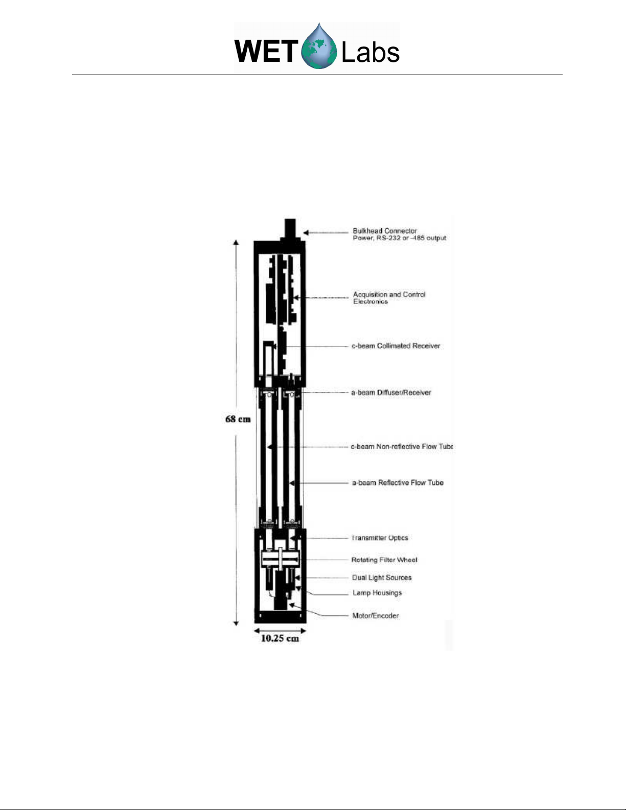
Before testing your instrument, familiarize yourself with the ac-9 and the ac-s (Figure 1).

Figure 1. Description of ac-9 components, many of which are shared with the ac-s.

ac meter Protocol (acprot) Revision N 21 May 2008 5

Both instruments consist of two pressure cans separated by a unistrut. The bottom pressure can
houses the transmitter optics and filter wheel. The top can contains the receiver optics and the
control electronics. Two removable plastic flow assemblies reside within the area separating the
two cans. These two assemblies define the flow volumes for the absorbance and transmittance
measurements.

Remove the black plastic flow tubes by sliding the flow tube sleeves towards the middle of the
flow tube. The flow tube will lift out, exposing the transmitter and detector windows on the
lower and upper flanges respectively. Be careful not to scratch the windows. The attenuation
tube is different than the absorption tube. Its flow chamber is black plastic and the two sleeves
on the tube are identical. This tube installs on the “c” side of the instrument (the side with the
identical looking windows). The “c” tube has no “up or down” orientation. The absorption flow
assembly is lined with a reflective quartz tube and one of the two sleeves is flat on top (the lip
present on all the other sleeves is missing). This tube installs on the “a” side of the instrument
that can be identified by the “a” detector that is on the upper flange and is the only window that
is clearly different from the other three (has a white diffuser where the other windows are
clear). The flow tube sleeve without the lip fits over the absorption window with diffuser, so
there IS an “up and down” orientation to the “a” tube.

You may want to mark the flow assemblies and their orientation with tape or marking pen
before using the instrument at sea so that there is no confusion when reinstalling the tubes after
cleaning your optics. Incorrect installation of the flow tubes will result in incorrect optical
measurements and water leaking around the sleeves because of improper o-ring seals (the
absorption window with detector has a different o-ring than the rest of the windows).

When re-installing the sleeves of the flow tubes, line up the white nylon set screws with the
grooves in the flow tubes. This will ensure that the water flow will not be blocked by the “tabs”
on the ends of the flow tubes.

The flow tube for the “c” channel may be considered optional as long as the detector is not
exposed to very intense ambient light (e.g., direct sunlight). This allows for the possibility of a
free path attenuation measurement when the flow tube is absent. Stray light is normally not a
concern with the “c” channel because of the collimating optics in the detector assembly. The
flow tube for the “a” channel is always required.

3.2 Testing

Before deploying the ac-9 or ac-s in the field you will want to test the unit to familiarize
yourself with the hardware and software, and to verify basic operation. Assuming that you are
using the factory-supplied software (WETView) to perform these tests, you will require the
following:

1. A clean, solid lab table or workbench;

2. The ac-9 or ac-s with test cable (or sea cable);

3. A power supply (the ac-9 and ac-s require 10–18 VDC);

4. A computer with WETView software installed for data acquisition.

6 ac meter Protocol (acprot) Revision N 21 May 2008

•

•

•

•

•

•

Installing WETView is very simple. You will need a 400 MHz or better PC running the
Windows 2000 or higher operating system with at least 10 Mb free hard disk space.

Create a directory or folder to copy the necessary files needed to install WETView onto your
machine. Copy the entire contents of the two disks you received with your ac-9 into this
directory on your computer. You should have the following files in your directory:

WETVIEW.001
WETVIEW.002
SETUP.EXE

WETPROCE.EXE
AC9XXXX.DEV
AIRXXXXX.CAL

One of the files copied is SETUP.EXE; run this program and follow the online instructions to
complete WETView installation.

Connect the factory supplied test cable to COMM port in your computer (or USB port via a serial to
USB converter). Connect the power leads to the power supply. The black lead is typically the V+
lead. Before connecting the cable to the instrument, use a multi-meter to check the input power.
Connect the ground probe to pin 1 on the pigtail connector (the centrally located pin). Connect the
hot probe to pin 4 (the pin directly opposite from pin 1). You should measure somewhere between
10–18 volts across these two pins. No other pins should have any voltage on them. Turn the power
supply off. Connect the pigtail to the instrument. Push the connector straight on to avoid damaging
the pins. Apply power to the instrument and allow it to warming up for about 30 s.

Run the WETView software by clicking on the icon in WINDOWS. When the interface is
displayed, you will need to provide a device file name (DEV file). Click on the <O> button in
the center top of the screen or choose “Open Device File” from the File Menu at the top left of
the screen. Browse to the folder containing the DEV file. The program will ask you to choose
the proper COMM port. Select COMM1 through COMM8 as appropriate. At this point, the
software will do some handshaking with the instrument and the “Start Logging” Button (or the
F1 key) can be used to start data collection. After 5–10 seconds, tabular data should be
displayed on the right side of the screen. A real time graph will begin to develop, using the
graph parameters set at the time. Please refer to the manual for the full details of running the
WETView software. After a short time, click on the F2 button. Data collection will stop and
you will be prompted for a file name to apply to the data if you should want to archive it. Press
ESC if you do not want to save the data. To quit the program, choose QUIT from the File menu,
not the (non-functioning) close button in the upper right of the program window. At this point
you have successfully completed a bench test of the instrument.

ac meter Protocol (acprot) Revision N 21 May 2008 7

3.3 Mounting

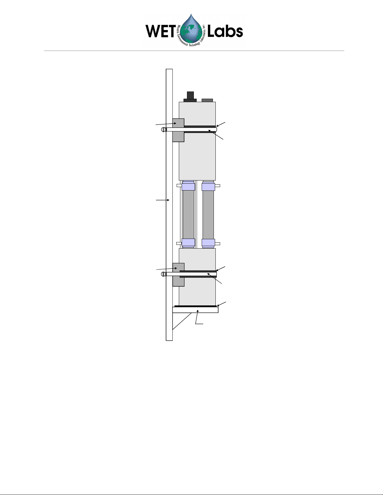
shouldbejustsnugtoavaoidapplyinganytorquetotheac-9.

Delrinor

PVCSaddle

Lowering Cage
Mounting Bar

Delrinor

PVCSaddle

Rubber
Sheet

Stainless

Hose Clamp

ac-9

Rubber
Sheet

Stainless

Hose Clamp

Rubber
Sheet

Steel Ledge
or Step

Note:Tightenupper hoseclamptightly. Lowerhoseclamp

Figure 2. Deployment cage mounting suggestion for ac-9 and ac-s.

The ac-9 and ac-s contains two optical paths that are sensitive to lateral and torsional stresses.
To ensure that the unit functions properly, it is important to minimize stresses when mounting
the unit to a frame. If possible, the ac device should be mounted vertical. These sensors can be
used in other orientations, but for the most accurate results field water calibrations should be
carried out when in the preferred deployment orientation to account for drifts associated with
small changes in the alignment of the optical paths. In the vertical orientation, it is preferable to
rest the bottom of the ac device on the cage framework and attach both the upper and lower
housings to the vertical framework of the cage (Figure 2). The housing attachments do not need
to be any tighter than required to hold the ac device to the cage as the main support is the

8 ac meter Protocol (acprot) Revision N 21 May 2008

bottom rest. If the ac device is to be mounted horizontally, it is critical to support both housings.
If the ac device is mounted horizontally and supported by only one housing, more substantial
deformation of the optical path will occur that may cause the unit to provide inaccurate
readings.

3.4 Plumbing and Tubing

It is important to ensure good flow through the ac meter flow tubes. The flow rate through the
instrument should be kept above 1 liter/min to resolve environmental changes over fine spatial
and temporal scales. This can be achieved by maximizing the tubing size and using a pump
such as the Sea-Bird Electronics SBE-5 running at a minimum 3000 rpm. The ac meter flow
tube sleeve nozzles are ½ in. to improve performance by potentially increasing the flow rate and
flushing through the flow assemblies, and to easily mate with the pump.

The detector for the absorption channels is very sensitive to external light, and the attenuation
detector can be affected when exposed to intense ambient light, so it best to eliminate the
leakage of any external light into the flow cells. This is accomplished by ensuring that all tubing
attaching to the flow cell sleeves is completely opaque or covered with opaque black tape. Note
that some electrical black tape is not completely opaque and can produce errors in absorption
readings at the surface.

Tygon tubing and other varieties may contain plasticizers that could possibly affect the optical
measurements if exposed to the sample for a significant amount of time. For short lengths of
tubing in typical applications using continuous flow, the type of tubing has not proved to be a
concern, as long as it is clean, laboratory grade. When using Tygon tubing, it is best to use a
thick-wall tube to prevent kinks in the tubing or collapse of the tubing due to possible pressure
differentials when pumping. Other types of tubing are available and include Teflon, Teflon­lined Tygon, and expensive grades of tubing without plasticizers. Many of the types of tubing
are rigid and care must be taken to prevent kinks from forming.

The plumbing should be installed in a manner that ensures bubbles cannot be trapped anywhere
in the system. A typical plumbing set-up is described. The upper and lower flow tube nozzles
are used for the outflows and inflows, respectively. Opaque tubing is attached to the intake
nozzles and dropped to the bottom of a deployment cage. The pump for the ac device should be
placed above the upper set of nozzles of the flow tubes. A “Y” fitting is used to merge the
outflows from the two flow cells into one flow that can be connected to the pump. On the
outflow from the pump a bubble degasser is typically installed. This device is an inverted “Y”
housing a Teflon insert with a small hole through the center that allows bubbles to escape the
system. It is required that the pump pull the water through the tubes rather than push it through.
The key consideration is that the plumbing configuration provides a clear path for bubbles to
escape the system when the sensor is deployed. If small bubbles are lodged in the flow cells, the
optical measurements will have errors. If bubbles become lodged in the pump, the pump will
stall and not work.
Separate intake tubes for the “a” and “c” sides of the instrument are recommended over using
“Y” or “T” fittings to separate the flow from a single intake tube. This is because evidence from
laboratory measurements indicates that a “Y” fitting may partition some particles preferentially
into one arm of the “Y” (Twardowski et al. 1999).

ac meter Protocol (acprot) Revision N 21 May 2008 9

In profiling applications where the sensor package may experience abrupt changes in rates of
descent and/or ascent, it is recommended that the inlet and outlet pressures of the flow system
be balanced. This is achieved by assuring that the entrance point and exit point of the tubing are
positioned at the same depth, i.e., a tube is installed that runs from the outflow leaving the pump
to the bottom of the cage where the sample intake tube is positioned (taking care not to orient
them too close together).

3.5 Attaching Prefilter to Remove the Particulate Fraction

An ac-9 or ac-s can be used to measure absorption by the dissolved fraction of water only. The
dissolved material responsible for this absorption is collectively known as colored dissolved
organic material (CDOM), “yellow matter,” or Gelbstoff. A capsule filter, typically with 0.2 µm
pore size, is attached in-line to either the “a” or “c” flow tube (or both) intake, so that particles
are removed prior to measurement. It is best to carefully cut the outer capsule of the filter off
with a saw (careful not to cut the filter pleats) to expose more filter surface area to the water.
Because CDOM is primarily composed of hydrophobic humic material, it is essential that the
capsule filter have a hydrophilic membrane. Otherwise, the filter may remove important
hydrophobic dissolved material.

Because scattering from the material present in the <0.2 µm fraction from natural waters
typically is negligible, attaching the filter to the intake of either the “a” or “c” side should yield
the same results. This is actually an excellent test to determine if your meter is operating as
expected. When deploying multiple ac devices, occasionally attaching prefilters to all the
meters is also an effective means of cross-calibrating the sensors.

To measure both the dissolved and particulate fractions of water independently, a dual ac-9 or
ac-s configuration may be assembled where one device has a prefilter (measures the dissolved
fraction only) and the other device does not (measures the dissolved + particulate fractions).
One ac device may be used to obtain the same set of data if successive casts are made, some
with the prefilter and some without. Extra care must be given to purging the system of air when
a filter is used, and there are other considerations to take into account, such as smearing of the
data because of longer (and variable as the filter captures more and more particles) time lags
(the time required for a sample to transit from the intake, through the filter, into the flow tube,
and undergo measurement). Using a high-speed pump (e.g., 4000-RPM SBE-5) is
recommended to minimize this effect. Even with a high-speed pump, however, time lags are
typically greater than 10 seconds (see section 5.3).

3.6 Deployment

The ac-9 and ac-s may be used in a variety of deployment modes. While emphasis and protocol
development has focused primarily upon profiling applications, the meter has also been used in
moored, lab flow-through, autonomous underwater vehicle, and towed applications. Each of
these modes requires some consideration in how best to optimize results from the meter. Below,
some of the most important issues are addressed with the primary modes of deployment.

3.6.1 Moorings

3.6.1.1 Anti-fouling—One of the most problematic aspects of a moored deployment of any
optical device is accumulation of biological growth on the optical surfaces. The enclosed
flow path of the ac-9 helps to retard biological fouling of the meter’s windows and the

10 ac meter Protocol (acprot) Revision N 21 May 2008

reflecting tube. Additional protection against biofouling may be provided by using copper
tubing on the inflow and outflow tubing of the flow tubes. The inhibitive effect is provided
by the slow dissolution of copper into the water between sampling events. Research has
shown that the use of copper tubing on the inflow and outflow tubing on an ac meter can
extend the measurement duration up to 60 days on coastal moorings (Manov, et al., 2004).

3.6.1.2 Warm-up—It is normally best to characterize and use the ac-9 or ac-s after a 5- to 10­minute warm-up from initially powering the meter. Moored deployments, however, typically
require sampling within thirty seconds after turning the unit on to conserve power. In order
to assure accuracy in the field, multiple samples should be collected with a clean dry system
in the lab, using the sample interval that is to be employed in the mooring. For best results,
the testing should occur at temperatures close to those to be found in the water. Once
multiple files have been collected, measurements in optically clean water (see Calibration,
section 4) may be made and compared to baseline zero values expected when applying the
device file (.dev) provided by the factory. Any offsets, which may or may not have a
temporal dependence while the instrument warms up, can later be applied to field
measurements as a correction.

3.6.1.3 Ground loops—The housing of the ac-9 and ac-s operates at ground potential,
effectively tying the instrument common to the seawater. Under normal circumstances this
should create no problems. However, depending upon other instrumentation attached to the
mooring, inadvertent current leakage paths, and ill-considered power schemes, there lies
potential for ground loops. In moored deployments, where packages can potentially be left
unattended for months, the ground loops can drain batteries, result in noisy measurements,
and damage instruments. While there is no set method for the determination and elimination
of ground loops the following steps provide general guidelines:

• Create a systems grounding diagram. Consider the seawater as a ground plane.

• Note all terminations to the seawater.

• Measure voltages across these terminations to determine possible voltage potentials.

Also check voltages across the instruments to the cage.

• If possible, immerse the package in salt water, and repeat the previous step

• A 2–3 day test deployment with instruments in the water could provide important

information on expected versus realized battery voltage decay.

• Mitigating a suspected ground loop is highly system specific. If you suspect a loop you

may wish to consult the factory for advice.

3.6.1.4 Plumbing—The inability to pre-purge moored deployments in near surface waters
makes it vitally important to properly plumb your system. If the tubing and meter orientation
do not facilitate rapid flushing of bubbles, air could easily become entrapped within the flow
assemblies. Also, in areas where the meter may be sampling large amounts of re-suspended
particulates, good flushing is critical to prevent sediment build-up within the meter. If
possible, pumping speeds may be set to higher speeds (4000–4500 RPM for the SBE-5) and
the incorporation of the larger nozzle diameter lock sleeves is recommended.

3.6.1.5 Calibration—Field calibrations immediately before and after mooring deployments
are essential to allow tracking of any drift due to fouling or possible instrument changes (see
section 4). The calibration should be performed as soon as possible after removal of the

ac meter Protocol (acprot) Revision N 21 May 2008 11

mooring from the water and after stored data is uploaded. Conducting a field water
calibration before cleaning the meter allows drift assessment in the “as-is” condition, which
will include drift due to both fouling and instrument changes. A second calibration after the
meter has been thoroughly cleaned will allow the user to track instrument specific drift. The
effects of fouling may be obtained by taking the difference between these two calibrations. In
situations where optically clean water is not available, obtaining an air tracking file after the
meter has been cleaned and dried will at least provide an indication of the meter stability
through the period of performance.

3.6.1.6 Power consumption and battery life—To assure that a viable data set is collected
during the entire period of deployment one must assure that they provide enough energy
capacity (batteries) to effectively operate throughout the duration. The ac-9 or ac-s with
pump will consume approximately 1 amp at 12 volts DC. Assuming a nominal on-time of
one minute for each sample, the instrument will use about 1/60 of an amp-hour during each
cycling. In addition, one must consider the power consumed by the data logger tied to the
instrument in both its “on” and “off” states. Batteries typically provide a rated capacity in
amp-hours, but this can mean different things for different types of batteries. For instance a
twelve volt, D-cell alkaline battery pack is rated around 12–14 amp hours, but due to the
near-linear decay rate of the batteries and the fact that this rating implies the amount of
energy that the battery might provide until it is at 50 percent voltage, the usable capacity is
only about 1/3 of the rated capacity. You must also take into account de-rating of the
capacity due to lower water temperatures. Near-zero degree Celsius temperatures could
reduce usable lifetimes by 30 percent. In generally, it is wise to provide ample over-capacity
in your power system. All things considered, the price of batteries is usually cheap compared
to the price of lost data.

3.6.2 Towed Bodies

3.6.2.1 Mounting—In mounting to a towed unit you must consider both the stability of the
device and the flight characteristics of the entire towed unit. While the latter consideration is
out of scope for this discussion, the former topic is straightforward. The mounting should
firmly secure the meter towards both ends, without applying excessive torque on the unit.
Neoprene-lined saddle clamps are recommended for this purpose. The clamps should be
securely anchored to the frame. In securing the meter, make sure that adequate clearance is
provided for plumbing and wiring. Because of size constraints, the meter usually must be
mounted near horizontal. As a result, it is imperative that a field water calibration be carried
out with the installed meter in the orientation expected during measurement to ensure the
meter is stable in its new orientation (see Section 4).

3.6.2.2 Plumbing—It is recommended that flow inlets and outlets be oriented so that the
hydrostatic pressure is equivalent, thus avoiding variable flow rates associated with variable
rates of ascent and descent (if applicable). This is most easily established by locating the inlet
and outlet hoses at the same level. Plumbing should be installed to allow the system to
completely purge all air when deployed. Because the meter may be mounted horizontally,
use bubble degassers and tubing to allow bubbles to escape. If possible, sending the package
down to 10 m or deeper before underway towing will help pressurize air out of the system. If
orientation and space constraints do not permit a plumbing configuration that enables air to
fully escape, plumb the meter in a manner that will allow air to escape when positioned in
another orientation. On initial deployment, use a tag line to allow immersion of the towed

12 ac meter Protocol (acprot) Revision N 21 May 2008