West Control Solutions KS98-1 User Manual

PMA Prozeß- und Maschinen-Automation GmbH

KS 98-1 Multi-function unit

Engineering manual

Valid from: 1.02.2011 Order number : 9499-040-82711

û

A publication of:

PMA
Prozeß- und Maschinen-Automation GmbH
P.O.Box 310 229 • D-34058 Kassel • Germany

All rights reserved.
No part of this document may be reproduced or
published in any form or by any means without
prior written permission from the copyright
owner.

Symbols used on the
instrument

Liability and warranty

Any information and notes in these operating instructions were
composed under consideration of the applicable regulations, the
present state of the art and our extensive know-how and experien
ce.

With special versions, additional ordering options or due to the la
test technical modifications, the actual scope of delivery may vary
from the descriptions and drawings in this manual.

For questions, please, contact the manufacturer.

a

Before starting to work with the instrument and be
fore commissioning, in particular, these operating
instructions must be read carefully!
The manufacturer cannot be held responsible for
damage and trouble resulting from failure to com
ply with the information given in this manual.

-

-

-

-

à

a

a

!

l

g

+

EU conformity marking

Caution, Follow the operating instructions!

Symbols in the text

Danger of injury

Danger for the instrument, or of faulty function

Danger of destroying electronic components due
to electrostatic discharge (ESD)

Additional information or reference to further
sources of information.

Important hint for avoiding frequent operator
faults.

This product may be subject to change due to im
provements of the product features in the course of
further development.

Copyright

This operating manual should be considered as confidential infor­mation, intended only for persons who work with the instrument.

Contraventions are subject to payment of damages. Further claims
reserved.

-

I-3

Content

I. Operating instruction .............................9

I-1 Description .......................................9

I-2 Safety notes .....................................10

I-3 Technical data ....................................12

I-4 Versions ........................................18

I-4.1 I/O-Modules ..................................19

I-4.2 Ex-factory setting ...............................19

I-4.3 Auxiliary equipment ..............................19

I-5 Mounting .......................................20

I-5.1 Function of wire-hook switches........................21

I-5.2 Retro-fitting and modific. of I/O-ext. (*watch connecting diagram).....22

I-5.3 I/O extension with CANopen .........................22

I-6 Electrical connections - Safety hints .......................23

I-6.1 Electromagnetic compatibility ........................23

I-6.2 Measurement earth connection........................23

I-6.3 RC protective circuitry ...........................24

I-6.4 Galvanic isolations ..............................24

I-6.5 General connecting diagram .........................24

I-6.6 Analog inputs .................................26

I-6.7 Digital in- and outputs.............................27

I-6.8 Connecting diagram i/o-modules .......................28

I-7 Commissioning ....................................29

I-8 Operation .......................................30

I-8.1 Front view ...................................30

I-8.2 Menu structure ................................31

I-8.3 Navigation, page selection ..........................32

I-8.4 Adjusting values................................33

I-9 Instrument settings in the main menu .......................34

I-9.1 CAN-Status ..................................34

I-9.2 Profibus-Status ................................34

I-9.3 ModC-Status .................................34

I-9.4 Calibration ...................................35

I-9.5 Online/Offline .................................35

I-10 Operating pages ...................................36

I-10.1 List display...................................36

I-10.2 Bargraph display................................36

I-10.3 Alarm display .................................37

I-10.4 Graphic trend curve ..............................37

I-10.5 Programmer ..................................38

I-10.6 Controller ...................................41

I-10.7 Cascade controller...............................46

I-11 Maintenance, test, trouble shooting........................48

I-11.1 Cleaning ....................................48

I-11.2 Behaviour in case of trouble .........................48

I-11.3 Shut-down ...................................48

I-11.4 Test engineering as basic equipment.....................48

I-11.5 I/O-Test ....................................50

I-3

II. Engineering-Tool ...............................51

II-1 Survey .........................................51

II-1.1 Scope of delivery ...............................51

II-2 Installation ......................................52

II-2.1 Hardware and software prerequisites ....................52

II-2.2 Software installation .............................52

II-2.3 Licencing....................................53

II-2.4 Software start .................................53

II-3 Menu reference to the engineering tool .....................54

II-3.1 Menu ‘File’...................................54

II-3.2 Menu ‘Edit’ ..................................60

II-3.3 Menu ‘Functions’ ...............................63

II-3.4 Menu ‘Fixed funct.’ ..............................63

II-3.5 Menu ‘Device’ .................................64

II-3.6 Menu ‘Options’ ................................65

II-3.7 Menu ‘Window’ ................................67

II-3.8 Menu ‘Help’ ..................................67

II-4 Engineering tool operation .............................68

II-4.1 Fundamentals of the engineering tool operation ..............68

II-4.2 Function block placement ...........................68

II-4.3 Function block shifting ............................68

II-4.4 Creating connections .............................69

II-4.5 Online operation................................71

II-4.6 Trend function .................................72

II-5 Building an engineering...............................77

II-6 Tips and tricks ....................................81

II-6.1 Function keys .................................81

II-6.2 Mouse key functions .............................82

II-6.3 Tips and tricks .................................83

III. Function blocks: ...............................89

III-1 Scaling and calculating functions.........................91

III-1.1 ABSV (absolute value (No. 01)) ........................91

III-1.2 ADSU ( addition/subtraction (No. 03)) ....................91

III-1.3 MUDI ( Multiplication / division (No. 05))...................92

III-1.4 SQRT ( square root function (No. 08)) .....................92

III-1.5 SCAL ( scaling (No. 09)) ............................93

III-1.6 10EXP (10s exponent (No. 10)) ........................93

III-1.7 EEXP (e-function (No. 11)) ...........................94

III-1.8 LN (natural logarithm (No. 12)) ........................94

III-1.9 LG10 (10s logarithm (No. 13)) .........................95

III-2 Non-linear functions.................................96

III-2.1 LINEAR (linearization function (No. 07)) ...................96

III-2.2 GAP (dead band (No. 20)) ...........................98

III-2.3 CHAR (function generator (No. 21)) ......................99

III-3 Trigonometric functions ..............................100

III-3.1 SIN (sinus function (No. 80)) .........................100

III-3.2 COS (cosinus function (No. 81)) .......................100

III-3.3 TAN (tangent function (No. 82)) .......................101

I-4

III-3.4 COT (cotangent function (No. 83)) ......................102

III-3.5 ARCSIN (arcus sinus function (No. 84)) ...................103

III-3.6 ARCCOS (arcus cosinus function (No. 85))..................104

III-3.7 ARCTAN (arcus tangent function (No. 86)) .................105

III-3.8 ARCCOT (arcus cotangent function (No. 87)) ................105

III-4 Logic functions ...................................106

III-4.1 AND (AND gate (No. 60)) ..........................106

III-4.2 NOT (inverter (No. 61)) ............................106

III-4.3 OR (OR gate (No. 62)) ............................107

III-4.4 BOUNCE (debouncer (No. 63)) ........................108

III-4.5 EXOR (exclusive OR gate (No. 64))......................108

III-4.6 FLIP (D flipflop (No. 65)) ...........................109

III-4.7 MONO (monoflop (No. 66))..........................110

III-4.8 STEP (step function for sequencing (No. 68)) ................111

III-4.9 TIME1 (timer (No. 69)) ............................112

III-5 Signal converters ..................................114

III-5.1 AOCTET (data type conversion (No. 02))...................114

III-5.2 ABIN (analog i binary conversion (No. 71)) ................115

III-5.3 TRUNC (integer portion (No. 72)) ......................117

III-5.4 PULS (analog pulse conversion (No. 73)) ..................118

III-5.5 COUN (up/down counter (No. 74)) ......................120

III-5.6 MEAN (mean value formation (No. 75)) ...................122

III-6 Time functions....................................124

III-6.1 LEAD ( differentiator (No. 50)) ........................124

III-6.2 INTE (integrator (No. 51)) ..........................126

III-6.3 LAG1 ( filter (No. 52)).............................128

III-6.4 DELA1 ( delay time (No. 53)) .........................129

III-6.5 DELA2 ( delay time (No. 54) ) ........................130

III-6.6 FILT ( filter with tolerance band (No. 55) ) ..................131

III-6.7 TIMER ( timer (No. 67) ) ...........................132

III-6.8 TIME2 ( timer (No. 70) ) ...........................133

III-7 Selecting and storage ...............................134

III-7.1 EXTR ( extreme value selection (No. 30)) ..................134

III-7.2 PEAK ( peak value memory (No. 31)).....................135

III-7.3 TRST ( hold amplifier (No. 32))........................136

III-7.4 SELC ( Constant selection (No. 33)) .....................136

III-7.5 SELD (selection of digital variables - function no. 06) ...........137

III-7.6 SELP ( parameter selection (No. 34)) ....................138

III-7.7 SELV1 ( variable selection (No. 35)) .....................139

III-7.8 SOUT ( Selection of output (No. 36)).....................140

III-7.9 REZEPT ( recipe management (No. 37)) ...................141

III-7.10 2OF3 ( 2-out-of-3 selection with mean value formation (No. 38)) .....143

III-7.11 SELV2 ( cascadable selection of variables (No. 39)) ............145

III-8 Limit value signalling and limiting ........................146

III-8.1 ALLP ( alarm and limiting with fixed limits(No. 40)).............146

III-8.2 ALLV ( alarm and limiting with variable limits (No. 41))...........148

III-8.3 EQUAL ( comparison (No. 42) )........................150

III-8.4 VELO ( rate-of-change limiting (No. 43) ) ..................151

III-8.5 LIMIT ( multiple alarm (No. 44)) .......................152

III-8.6 ALARM ( alarm processing (No. 45) )

....................153

I-5

III-9 Visualization .....................................154

III-9.1 TEXT (text container with language-dependent selection (No. 79)) ....154

III-9.2 VWERT ( display / definition of process values (No. 96) )..........156

III-9.3 VBAR ( bargraph display (No. 97) )......................161

III-9.4 VPARA ( parameter operation (No. 98) ) ...................164

III-9.5 VTREND ( trend display(No. 99) ) ......................166

III-10 Communication ...................................169

III-10.1 L1READ ( read level1 data(No. 100) ) ....................169

III-10.2 L1WRIT ( write level1 data (No. 101)) ....................170

III-10.3 DPREAD ( read level1 data via PROFIBUS (No. 102) ) ............171

III-10.4 DPWRIT ( write level1 data via PROFIBUS (No. 103)) ............172

III-10.5 MBDATA (read and write parameter data via MODBUS - no. 104) ....173

III-11 I/O extensions with CANopen...........................175

III-11.1 RM 211, RM212 and RM213 basic modules ................175

III-11.2 C_RM2x (CANopen fieldbuscoupler RM 201 (No. 14)) ...........176

III-11.3 RM_DI (RM 200 - (digital input module (No. 15)) ..............177

III-11.4 RM_DO (RM 200 - digital output module (No. 16)) .............177

III-11.5 RM_AI (RM200 - analog input module (No. 17)) ..............178

III-11.6 RM_AO (RM200 - analog output module (No. 18)) .............180

III-11.7 RM_DMS (strain gauge module (No. 22)) ..................181

III-12 KS 98-1- KS 98-1 cross communication (CANopen) ..............183

III-12.1 CRCV (receive mod. block no's 22,24,26,28 (No.56)) ............183

III-12.2 CSEND (Send mod. blockno.'s 21, 23, 25, 27 - (No. 57)) ..........184

III-13 Connection of KS 800 and KS 816 .........................185

III-13.1 C_KS8x (KS 800 and KS 816 node function - (No. 58)) ...........186

III-13.2 KS8x (KS 800/ KS 816 controller function - (No. 59)) ............187

III-14 Description of KS 98-1 CAN bus extension ...................189

III-14.1 CPREAD (CAN-PDO read function (No. 88)) .................193

III-14.2 CPWRIT (CAN-PDO write function (No. 89)) ................194

III-14.3 CSDO (CAN-SDO function (No. 92)) ....................195

III-15 Programmer .....................................201

III-15.1 APROG ( analog programmer (No. 24)) / APROGD ( APROG data (No. 25)) . 201
III-15.2 DPROG ( digital programmer (No. 27)) / DPROGD ( DPROG data(No. 28)) . 219

III-16 Controller.......................................223

III-16.1 CONTR (Controllerfunction with one parameterset (No. 90)) ........223

III-16.2 CONTR+ (Controllerfunction with six parametersets (No. 91)) .......224

III-16.3 Parameter and Konfiguration for CONTR, CONTR+ .............226

III-16.4 Control behaviour ..............................228

III-16.5 Optimizing the controller...........................240

III-16.6 Empirical optimization ............................241

III-16.7 Self-tuning r controller adaptation to the process ............242

III-16.8 PIDMA (Control function with particular self-tuning behaviour (No. 93) .....247

III-16.9 Parameter and configuration for PIDMA ..................250

III-16.10 Controller characteristics and self-tuning with PIDMA ...........252

III-16.11 Controller applications: ...........................256

III-16.12 Setpoint functions ..............................260

III-16.13 Process value calculation ..........................265

III-16.14 Small controller ABC ...........................271

III-17 Inputs .........................................274

I-6

III-17.1 AINP1 ( analog input 1 (No. 08)) .......................274

III-17.2 AINP3...AINP5 ( analog inputs 3...5 (No. 112...114) ) ............281

III-17.3 AINP6 ( analog input 6 (No. 115)) ......................282

III-17.4 DINPUT ( digital inputs (No. 121)) ......................285

III-18 Outputs ........................................286

III-18.1 OUT1 and OUT2 ( process outputs 1 and 2 (No. 116, 117)).........286

III-18.2 OUT3 ( process output 3 (No. 118)).....................287

III-18.3 OUT4 and OUT5 ( process outputs 4 and 5 (No. 119...120))........288

III-18.4 DIGOUT ( digital outputs (No. 122)).....................289

III-19 Additional functions ................................290

III-19.1 LED (LED display (No. 123)).........................290

III-19.2 CONST ( constant function (No. 126) )...................291

III-19.3 INFO ( information function (No. 124) )...................292

III-19.4 STATUS ( status function (No. 125)).....................293

III-19.5 CALLPG (Function for calling up an operating page (no. 127)) .......296

III-19.6 SAFE ( safety function (No. 94)).......................297

III-19.7 VALARM (display of all alarms on alarm operating pages (function no. 109)298

III-20 Modular I/O - extension-modules ........................300

III-20.1 TC_INP (analog input card TC, mV, mA) ...................300

III-20.2 F_Inp (frequency/counter input) .......................302

III-20.3 R_Inp (analog input card ) ..........................303

III-20.4 U_INP (analog input card -50...1500mV, 0...10V) ..............305

III-20.5 I_OUT (analog output card 0/4...20mA, +/-20mA) .............307

III-20.6 U_OUT (analog output card 0/2...10V, +/-10V) ...............308

III-20.7 DIDO (digital input/output card) .......................309

III-21 Function management ...............................310

III-21.1 Memory requirement and calculation time .................310

III-21.2 Sampling intervals ..............................311

III-21.3 EEPROM data ................................311

III-22 Examples.......................................312

III-22.1 Useful small engineerings ..........................312

III-22.2 Controller applications ............................313

III-23 Index .........................................314

I-7

Preface

This manual consists of three parts.

I. Operating instructions

II. Engineeringtool description

III. Function block description

Section I holds the required information for identification, mounting, connection and electrical commissioning of the
unit under consideration of safety notes of the application and environmental conditions.

The basic principles of operation are explained: Controls and indicators, menu structure and navigation with the cursor,
selection of sub-menus and properties as well as adjustment of e.g. s and parameters.

Section II comprises the handling of the engineering-tool, the building of a simple engineering and transmission to the
KS 98-1.

9499-040-82711

+

+

Section III presents the particular fnction blocks in detail.

For functional commissioning, additional descriptions are required; please, order them separately or load them from
the PMA homepage: www.pma-online.de

As the functions provided in KS 98-1 are composed individually for each application using an Engineering Tool
ET/KS 98, entire comprehension of the operating functions requires the relevant Project description with the Enginee ­ring !

Supplementary documentation:

PROFIBUS-protocol (GB) 9499-040-82811
ISO 1745-protocol (GB) 9499-040-82911

I-8

9499-040-82711 Description

I Operating instruction

I-1 Description

1

2

KS 98-1 advanced

4

3

Fig. 1 Frontview

The instrument is a compact automation unit the function of which can be configured freely by means of function
blocks. Each unit contains a comprehensive function library for selection, configuration, parameter setting and connec ­tion of max. 450 function blocks by means of an engineering tool.

I.e. complex mathematical calculations, multi-channel control structures and sequence controllers can be realized in a
single unit.

Various operating pages are indicated via the front-panel LCD matrix display, e.g.

Numeric input and output of analog and digital signals, values and parameters as well as

w

full-graphics display of bargraphs, controllers, programmers and trends.

w

Display colour red / green and direct / inverse display can be switched over dependent on event, or by operation

w

dependent on the engineering.

Dependent on version, the basic unit is equipped with analog and digital inputs, outputs and relays.

Additional inputs and outputs are available either with option C or “modular option C”, which contains four sockets for
various I/O modules.

Optionally, the unit may be equipped with 2 additional communication interfaces:

Option B: serial TTL/RS422 interface or Profibus-DP

w

Option CAN: CANopen-compliant interface port for the I/O extension with modular I/O system RM200

w

I-9

Safety notes 9499-040-82711

The user is responsible that the instrument is operated only by

I-2 Safety notes

This section provides a survey of all important safety aspects: op
timum protection of personnel and safe, trouble-free operation of
the instrument.

Additionally, the individual chapters include specific safety notes
for prevention of immediate hazards, which are marked with sym
bols. Moreover, the hints and warnings given on labels and in
scriptions on the instruments must be followed and kept in
readable condition continuously.

General

Software and hardware are programmed or developed in compli
ance with the state of the art applicable at the time of develop
ment, and considered as safe.

Before starting to work, any person in charge of work at the prod
uct must have read and understood the operating instructions.

trained and authorized persons. Maintenance and repair may be
done only by trained and specialized persons who are familiar

-

with the related hazards.

Operation and maintenance of the instrument are limited to reli
able persons. Any acts susceptible to impair the safety of persons
or of the environment have to be omitted. Any persons who are
under effect of drugs, alcohol or medication affecting reaction are

­precluded from operation of the instrument.

-

Instrument Safety

This instrument was built and tested according to VDE 0411 /
EN61010-1 and was shipped in safe condition. The unit was
tested before delivery and has passed the tests required in the

­test plan.

-

In order to maintain this condition and to ensure safe operation,
the user must follow the hints and warnings given in these safety

­notes and operating instructions.

-

The plant owner is recommended to request evidence for knowl
edge of the operating instructions by the personnel.

-

Correct use for intended application

The operating safety is only ensured when using the products cor­rectly for the intended application. The instrument can be used as
a multiple function controller for open and closed control loops in
industrial areas within the limits of the specified technical data
and environmental conditions.

Any application beyond these limits is prohibited and considered
as non-compliant.

Claims of any kind against the manufacturer and /or his lawful
agents, for damage resulting from non-compliant use of the instru
ment are precluded, liability is limited to the user.

User responsibility

The user is responsible:

for keeping the operating manual in the immediate vicinity

w

of the instrument and always accessible for the operating
personnel.

for using the instrument only in technically perfect and safe

w

condition.

Apart from the work safety notes given in these operating instruc
tions, compliance with the generally applicable regulations for
safety, accident prevention and environment protection is compul
sory.

The user and the personnel authorized by the user are responsible
for perfect functioning of the instrument and for clear definition of
competences related to instrument operation and maintenance.
The information in the operating manual must be followed com
pletely and without restrictions!

-

The unit is intended exclusively for use as a measuring and control
instrument in technical installations.

The insulation meets standard EN 61010-1 with the values for
overvoltage category, degree of contamination, operating voltage
range and protection class specified in the operating instructions /
data sheet.

The instrument may be operated within the specified environmen­tal conditions (see data sheet) without impairing its safety.

The instrument is intended for mounting in an enclosure. Its con­tact safety is ensured by installation in a housing or switch cabi­net.

Unpacking the instrument

­Remove instrument and accessories from the packing. Enclosed

standard accessories:

–

operating notes or operating instructions

–

fixing elements.

Check, if the shipment is correct and complete and if the instru
ment was damaged by improper handling during transport and
storage.

!

-

We recommend to keep the original packing for shipment in case

­of maintenance or repair.

Warning!
If the instrument is so heavily damaged that safe operati
on seems impossible, the instrument must not be taken
into operation.

-

-

I-10

9499-040-82711 Safety notes

Mounting

Mounting is done in dustfree and dry rooms.
The ambient temperature at the place of installation must not ex

ceed the permissible limits for specified accuracy given in the
technical data. When mounting several units with high packing
density, sufficient heat dissipation to ensure perfect operation is
required.

For installation of the unit, use the fixing clamps delivered with
the unit.

The sealing devices (e.g. sealing ring) required for the relevant
protection type must also be fitted.

Electrical connections

All electrical wiring must conform to local standards
(e.g. VDE 0100 in Germany). The input leads must be kept separate
from signal and mains leads.

The protective earth must be connected to the relevant terminal
(in the instrument carrier). The cable screening must be connected
to the terminal for grounded measurement. In order to prevent
stray electric interference, we recommend using twisted and
screened input leads.

The electrical connections must be made according to the relevant
connecting diagrams.

See electrical safety, page 23

Electrical safety

The insulation of the instrument meets standard EN 61 010-1 (VDE
0411-1) with contamination degree 2, overvoltage category III,
working voltage 300 V r.m.s. and protection class I.

Galvanically isolated connection groups are marked by lines in the
connecting diagram.

Commissioning

Before instrument switch- on, ensure that the rules given below
were followed:

Ensure that the supply voltage corresponds to the specifica

w

tion on the type label.

All covers required for contact safety must be fitted.

w

Before instrument switch- on, check if other equipment and

w

/ or facilities connected in the same signal loop is / are not
affected. If necessary, appropriate measures must be taken.

On instruments with protection class I, the protective earth

w

must be connected conductingly with the relevant terminal
in the instrument carrier.

Operation

Switch on the supply voltage. The instrument is now ready for op
eration. If necessary, a warm- up time of approx. 1.5 min. should

­be taken into account.

a

Warning !
Any interruption of the protective earth in the in
strument carrier can impair the instrument safety.
Purposeful interruption is not permissible.
If the instrument is damaged to an extent that
safe operation seems impossible, shut it down
and protect it against accidental operation.

Shut- down

For permanent shut- down, disconnect the instrument from all
voltage sources and protect it against accidental operation.

Before instrument switch- off, check that other equipment and / or
facilities connected in the same signal loop is / are not affected. If
necessary, appropriate measures must be taken.

Maintenance and modification

The instrument needs no particular maintenance.
Modifications, maintenance and repair may be carried out only by

trained, authorized persons. For this, the user is invited to contact
the service.

For correct adjustment of wire-hook switches (page 21 ) and for in­stallation of modular option C, the unit must be withdrawn from
the housing.

a

Before carrying out such work, the instrument must be discon
nected from all voltage sources.

After completing such work, re- shut the instrument and re-fit all

­covers and components. Check, if the specifications on the type la
bel are still correct, and change them, if necessary.

Warning!
When opening the instruments, or when remo
ving covers or components, live parts or termi
nals can be exposed.

Explosion protection

Non-intrinsically safe instruments must not be operated in explo
sion-hazarded areas. Moreover, the output and input circuits of
the instrument / instrument carrier must not lead into explo
sion-hazarded areas.

-

-

-

-

-

-

-

-

The instrument must be operated only when mounted in its

w

enclosure.

I-11

Technical data 9499-040-82711

I-3 Technical data

General

Housing

Plug-in module, inserted from front.
Material: Makrolon 9415, flame-retardant, self-extinguishing
Flammability class: UL 94 VO

Front-panel / display

160 x 80-dot LCD matrix display
4 LEDs, 4 foil-covered keys

Front interface port (standard)

Front-panel socket for PC adapter
(see „Accessories“ page 19).

Protection mode

(to EN 60 529, DINVDE 0470)
Front: IP 65
Housing: IP 20
Terminals: IP 00

Safety tests

Complies with EN 61 010-1

Overvoltage category: III

w

Contamination class: 2

w

Working voltage range: 300 VAC

w

Protection class: I

w

Electrical connections

Screw terminals for conductor cross-section from 0,5 - 2,5 mm

Mounting method

Panel mounting with 4 fixing clamps at top/bottom

Mounting position

Not critical

Weight

Approx. 0.75 kg with all options

Environmental conditions

Permissible temperatures

For operation: 0...55°C
For specified accuracy: 0...60°C, optionC
For UL-Devices: Operation and protected operation 0...50°C
Storage and transport: –20...60 °C

Temperature effect: £ 0.15% / 10 K

Climatic category

KUF to DIN 40 040
Relative humidity: £ 75% yearly average, no condensation

Shock and vibration

Vibration test Fc: To DIN 68-2-6 (10...150 Hz)
Unit in operation: 1g or 0.075 mm,
Unit not in operation: 2g or 0.15 mm
Shock test Ea:To DIN IEC 68-2-27 (15g, 11 ms)

2

DIN EN 14597

The device may be used as temperature control and limiting equip
ment according to DIN EN 14597.

CE marking

Meets the EuropeanDirectives regarding „Electromagnetic Compa
tibility“ and „Low-voltage equipment“(r page 23)

The unit meets the following European guidelines:

q

Electromagnetic compatibility (EMC): 89/336/EEC
(as amended by 93/97/EEC)

q

Electrical apparatus (low-voltage guideline):
73/23/EEC (as amended by 93/68/EEC).

Evidence of conformity is provided by compliance with EN 61326-1
and EN 61010-1

cULus certification

cULus-certification

(Type 1, indoor use) File: E 208286

a

RC protective circuitry must be fitted with inducti
ve load !

-

-

-

I-12

9499-040-82711 Technical data

Connections

Depending on version and selected options, the following inputs
and outputs are available:

DI DO AI AO

4 relays

di1*

or

2 relays

+

2AO

OPTION B

OPTION C*

or

modular

OPTION C*

Not available with option CAN!

*

di2*

di1*
di2*

di3
di4

di5
di6
di7

di8

di9

di10
di11
di12

OUT1
OUT2
OUT4

OUT5

OUT4
OUT5

do1
do2
do3

do4

do5
do6

INP1
INP5
INP6

INP1
INP5
INP6

––

INP3
INP4

Depending on module type

–

OUT1
OUT2

OUT3

Inputs

Resistance thermometer

Pt 100 to DIN IEC 751, and temperature difference2xPt100

Range Error Resolution

–200.0...250.0 °C £ 0.5 K 0.024 K

–200.0...850.0 °C £ 1.0 K 0.05 K
2 x –200.0...250.0 °C £ 0.5 K 0.024 K
2 x –200.0...250.0 °C £ 0.1 K 0.05 K

Linearization in °C or ° F
Two wire connection with compensation or three-wire connection

without.
Two-wire connection with lead resistance adjustment.
Lead resistance: £ 30 W per lead
Sensor current: £ 1mA
Input circuit monitoring for sensor/lead break, and lead short circuit.

Potentiometric transducer

R

incl. 2 x R

total

L

0...500 W£0.1 % £ 0.02 W

Resistance-linear
Sensor current: £ 1mA
Matching/scaling with sensor connected.
Input circuit monitoring for sensor/lead break, and lead short circuit.

Error Resolution

Universal input INP1

Limiting frequency: fg=1Hz,Measurementcycle: 200 ms

Thermocouples

according to DIN IEC 584

Type Range Error Resolution
L –200...900°C £ 2K 0,05 K
J –200...900°C £ 2 K 0,05 K
K –200...1350°C £ 2 K 0,072 K
N –200...1300°C £ 2 K 0,08 K
S –50...1760°C £ 3 K 0,275 K
R –50...1760°C £ 3 K 0,244 K

1)

B

(25)400...1820°C £ 3 K 0,132 K

T –200.. .400°C £ 2 K 0,056 K

2)

W(C)
E –200... 900°C £ 2 K 0,038 K

With linearization (temperature-linear in °C or °F)
Input resistance: ³ 1MW
Cold-junction compensation (CJC): built in

Input circuit monitor:

Current through sensor: £ 1mA
Reverse-polarity monitor is triggered at 10 °C below span start.

Additional error of internal CJC

£ 0.5 K per 10 K terminal temperature External temperature
selectable: 0...60 °C or 32...140 °F

0...2300°C £ 2 K 0,18 K

*

1 ) from 400 °C

*

2 ) W5Re/W26Re

Resistance input

Range Error Resolution

0...250 W£0.25 W < 0.01 W

0...500 W£0.5 W < 0.02 W

Direct current 0/4...20mA

Range Error Resolution
0/4...20 mA £ 0.1 % £ 0.8 mA

Input resistance: 50 W
Input circuit monitor with 4...20mA: triggered when I £ 2mA

Direct voltage

Range Error Resolution
0/2...10 V £ 0.1 % £ 0.4 mV

Input resistance ³ 100 kW

I-13

Technical data 9499-040-82711

Signal input INP5
Differential amplifier input

Up to 6 controllers can be cascaded, if there is no other galvanic
connection between them. If there is, only 2 inputs can be cascaded.

Direct current and voltage

Technical data as for INP1, except for:
Limiting frequency: = 0.25 Hz, Measurement cycle: 800 ms
Input resistance (voltage): ³ 500 kW

Signal input INP6

Limiting frequency: = 0.5 Hz, Measurement cycle: 400 ms

Potentiometric transducer

Technical data as for INP1, except for:

R

inkl. 2 x RL Error Resolution

total

0...1000 W£0.1 % £ 0.04 W

Direct current 0/4...20 mA

Technical data as for INP1

Signal inputs INP3, INP4 (option C)

Galvanically-isolated differential amplifier inputs.
Limiting frequency: fg = 1 Hz, Measurement cycle: 100 ms

Direct current

Technical data as for INP1, except Ri = 43 W

Outputs

Relay outputs (OUT4, OUT5)

Relays have potential-free change-over contacts.
Max. contact rating:
500 VA, 250 V, 2 A with 48...62 Hz, cosj³0,9
Minimum rating: 12 V, 10 mA AC/DC
Number of switching cycles electrical: for I = 1A/2A ³ 800,000 /

500,000 (at ~ 250V / (resistive load))

When connecting a contactor to a relay output, RC

!

protective circuitry to specification of the contactor
manufacturer is required. Varistor protection is not
recommended!

Outputs OUT1, OUT2

Relay or current/logic signal, depending on version:

OUT1, OUT2 as current outputs

Galvanically isolated from the inputs
0/4...20 mA, selectable
Signal range: 0...22 mA
Resolution: £ 6mA (12 bits)
Error: £ 0.5%
Load: £ 600 W
Load effect: < 0.1%
Limiting frequency: approx. 1 Hz Output cycle: 100ms

Control inputs di1...di12

di1, di2: standard
di3...d7: Option B
di8...di12: Option C

Opto-coupler

Nominal voltage: 24 VDC, external
Current sink (IEC 1131 Type 1)
Logic „0“ (Low): –3...5 V, Logic „1“ (High): 15...30 V
Current demand: approx. 6 mA (for galvanic connections and isola

tion see page 25).

Built-in transmitter supply (optional)

Can be used to energize a two-wire transmitter or up to 4
opto-coupler inputs.Galvanically isolated.

Output: ³ 17.5 VDC, max. 22 mA
Short-circuit proof.

Factory setting

The transmitter supply is available at terminals A12 and A14

+

See page 25, Configuration see page 21

OUT1, OUT2 as logic signal

0/³ 20 mA with a load ³ 600 W
0 / > 12 V with a load ³ 600 W

Output OUT3 (Option C)

Technical data as for OUT1, OUT2, as current output

Control outputs do1..do6

Galvanic isolated Opto-coupler outputs, galvanic isolation see

­page 25 and text.

Grounded load: common positive control voltage

Switch rating: 18...32 VDC; Imax £ 70 mA
Internal voltage drop: £ 0.7V with I

Protective circuit: thermal, switches off with overload.
Supply 24 V DC external
Residual ripple £ 5%

ss

max

I-14

9499-040-82711 Technical data

Modular Option C

Each module has two channels which can be configured independently.

A/D-Converter

Resolution: 20,000 (50Hz) or 16,667 (60Hz) steps for the selected
measuring range.

Conversion time: 20ms (50Hz) or 16.7ms (60Hz).

D/A-Converter

Resolution:12Bit
Refresh-Rate: 100 ms

Cut-off frequency

Analog: fg=10Hz
Digital: fg=2Hz
Measurement cycle: 100 ms per module

R_INP Resistive input module

(9407-998-0x201)
Connection method: 2, 3 or 4-wire circuit (with 3 und 4-wire con

nection, only one channel can be used).

Sensor current:

£ 0,25mA

Resistance thermometer

Type Range °C Overall error Resolution K/Digit
Pt100 -200...850°C £ 2 K 0,071
Pt100 -200...100°C £ 2 K 0,022
Pt1000 -200...850°C £ 2 K 0,071
Pt1000 -200...100°C £ 2 K 0,022
Ni100 -60...180°C £ 2 K 0,039
Ni1000 -60...180°C £ 2 K 0,039

Linearization: in °C oder °F

Lead resistance

Pt (-200...850°C): £ 30
Pt (-200...100°C), Ni: £ 10

Lead resistance compensation

3 and 4-wire connection: not necessary.
2-wire connection: compensation via the front with short-circuited

sensor. The calibration values are stored in a non-volatile memory.

Lead resistance effect

3 and 4-wire connection: negligible

Sensor monitoring

Break: sensor or lead. Short-circuit: triggers at 20 K below mea
suring range.

Resistance / Potentiometer

Range R

0...160 W

0...450 W

0...1600 W

0...4500 W

ges

/ W

W per lead

W per lead

Overall error

£ 1% 0,012
£ 1% 0,025
£ 1% 0,089
£ 1% 0,025

-

Resolution W/Digit

Characteristic: resistance-linear
Lead resistance or 0%/100% compensation:

via the front with short-circuited sensor. The calibration values are
stored in a non-volatile memory.

Variable resistance (only 2-wire connection): compensation for 0%

w

Potentiometer: compensation for 0% and 100%

w

Lead resistance effect

3 and 4-wire connection: negligible

Sensor monitoring:

break: sensor or lead

TC_INP Thermocouple, mV, mA Module

(9407-998-0x211)

Thermocouples

To DIN IEC 60584 (except L, W/C, D)

Type Range

L

­J

K

N
S
R

(1)

B

T

W(C)

D

E

*

(1) Values apply from 400°C

-200...900°C

-200...900°C

-200...1350°C

-200...1300°C

-50...1760°C

-50...1760°C

(25) 400...1820°C

-200...400°C

0...2300°C

0...2300°C

-200...900°C

Overall

error

£ 2 K 0,080
£ 2 K 0,082
£ 2 K 0,114
£ 2 K 0,129
£ 3 K 0,132
£ 3 K 0,117
£ 3 K 0,184
£ 2 K 0,031
£ 2 K 0,277
£ 2 K 0,260
£ 2 K 0,063

Linearization:in°Cor°F
Linearity error: negligible

Input resistance:

³1MW

Temp. compensation (CJC): built in

£ 0.5K/10K

Error:
External CJC possible: 0...60 °C or. 32...140 °F
Source resistance effect: 1mV/kW

Sensor monitoring:

Sensor current:

£ 1mA

Reversed polarity monitor: triggers at 10K below measuring range

mV input

Range

0...30 mV

0...100 mV

0...300 mV

Input resistance: ³1MW
Break monitoring: built in. Sensor current: £1mA

Overall error Resolution

£ 45 mV 1,7 mV
£ 150 mV 5,6 mV
£ 450 mV 17 mV

K/Digit

I-15

Technical data 9499-040-82711

mA input

Range
0/4...20 mA

Input resistance:10W
Break monitor:<2mA (only for 4...20 mA)
Over range monitor: >22mA

Overall error

£ 40 mA 2 mA

Resolution

U_INP High-impedance voltage input

(9407-998-0x221)

Range

-50...1500 mV

0...10 V

Characteristic: voltage-linear
Input resistance: >1G
Source resistance effect: £ 0,25 mV/MW
Sensor monitoring: none

Overall error Resolution mV/Digit

£ 1,5 mV 0,09

£ 10 mV 0,56

W

U_OUT Voltage output module

(9407-998-0x301)

Signal ranges: 0/2...10V, -10...10V configurable
Resolution: approx.. 5.4 mV/digit
Load: ³ 2kW

Load effect : £ 0.1%

I_OUT Current output module

(9407-998-0x311)

Signal ranges: 0/4...20mA, -20...20mA configurable by channel
Resolution: ca. 11mA/Digit
Load: £ 400 W

Load effect: £ 0.1%/100W

F_INP Frequency/counter Module

(9407-998-0x411)

Current sink: to IEC 1131 Type 1

Logic „0“: -3...5V
Logic „1“: 15...30V

Galvanic isolation: via Opto-couplers
Nominal voltage: 24 VDC external
Input resistance:12k
Selectable functions:

Control input (2 channels)

w

Pulse counter (2 channels)

w

Frequency counter (2 channels)

w

Up/down counter (1 channel)

w

Quadrature counter (1 channel)

w

Frequency range:
Signal shape: any (square 1:1 with 20kHz)
Gate time: 0.1...20s adjustable (only relevant with frequency mea

surement)

W

£ 20 kHz

-

Influencing factors

Temperature effect: £ 0,1%/10K
Supply voltage: negligible
Common mode interference: negligible up to 50 Vrms
Series mode interference: negligible up to 300 mVrms (TC),

30 mVrms (RT), 10 Vrms (U), 5 Vrms (F)

CAN I/O extension

The unit offers a port conforming to CANopen for connection of
the RM 200 system and of KS 800 or additional KS 98-1 units with
max. five CAN nodes.

DIDO Digital I/O Module

(9407-998-0x401)

Number of channels: 2 (configurable as input or output by channel)

Input

Current sink: to IEC 1131 Type 1)
Logic „0“: -3...5V, Logic „1“: 15...30V

Measurement cycle: 100 ms
Galvanic isolation : via opto-couplers
Nominal voltage: 24 VDC external

Input resistance:5k

W

Output

Grounded load (common positive control voltage)

Switch rating: 18...32 VDC;
Internal voltage drop:
Refresh-Rate: 100 ms
Galvanic isolation : via opto-couplers
Protective circuit: thermal, switches off with overload.

I-16

£70 mA

£ 0.7 V

+
+

Control inputs di1 and di2 are not available !

Modular option C is not available

Power supply

Dependent on version:

Alternating current

90...250 VAC
Frequency: 48...62 Hz
Power consumption: approx. 17,1 VA; 9,7 W (max. configuration).

Universal current 24 V UC

24 VAC, 48...62 Hz/24 VDC
Tolerance: +10...–15% AC 18...31.2 VDC
Power consumption AC: approx. 14.1 VA; 9.5 W
DC: 9,1 W (max. Configuration).

9499-040-82711 Technical data

Behaviour after power failure

Storage in non-volatile EEPROM for structure, configuration, pa
rameter setting and adjusted setpoints.

Storage in a capacitor-buffered RAM (typ. > 15 minutes) for data
of time functions (programmers, integrators, counters, ...)

-

Real-time clock(Option B, RS 422)

Buffer capacitor provides back-up for at least 2 days (typical).

Bus interface (Option B)

TTL and RS422 / 485-interface

Galvanically isolated, choice of TTL or
RS 422/485 operation.

Number of multi function unitsper bus:

With RS 422/485: 99
With TTL signals: 32 interface modules (9404 429 980x1). Address

range ((00...99)See Documentation 9499-040-82911) .

PROFIBUS-DP interface

According to EN 50 170, Vol. 2.
Reading and writing of all process data, parameters, and configu-

ration data.

Transmission speeds and cable lengths

automatic transm. speed detection, 9,6 kbit/s ...12 Mbit/s

Addresses

0...126 (factory setting: 126).Remote addressing is possible.

Other functions

Sync and Freeze

Terminating resistors

Internally selectable with wire-hook switches.

Cable

According to EN 50 170, Vol. 2 (DIN 19 245T3).

Required accessories

Engineering Set PROFIBUS-DP, consisting of:

GSD file, Type file

w

PROFIBUS manual (9499-040-82911)

w

Function block(s) for Simatic S5/S7

w

Electromagnetic compatibility

Complies with EN 50 081-2 and EN 50 082-2.

Electrostatic discharge

Test to IEC 801-2,
8 kV air discharge
4 kV contact discharge

High-frequency interference

Test to ENV 50 140 (IEC 801-3)

80...1,000 MHz, 10 V/m
Effect: £ 1%

HF interference on leads

Test to ENV 50141 (IEC 801-6)

0.15...80 MHz, 10 V
Effect: £ 1%

Fast pulse trains (burst)

Test to IEC 801-4
2 kV applied to leads for supply voltage, and signal leads.

Effect: £ 5%resp. restart

High-energy single pulses (surge)

Test to IEC 801-5
1 kV symmetric or 2 kV asymmetric on leads for supply voltage.

0.5 kV symmetric or 1 kV asymmetric on signal leads.

I-17

Versions 9499-040-82711

I-4 Versions

The instrument version results from the combination of various
variants from the following table.

Fig. 2

Please mindfootnotes!
KS98-1 with screw terminals
only!

KS 98 Standard

KS

1

89

-

-

000

-

0

BASIC UNIT

POWER SUPPLY AND

CONTROL OUTPUTS

OPTION B

INTERFACE

OPTION

(standard)

OPTION

(modular)

SETTING

KS 98 with transmitter power supply
KS 98 with CANopen I/O

1)

90...250V, AC 4 relays
24V UC, 4 relays 1

90...250V AC 2 relays+ 2 mA/logic, 4
24V UC, 2 + 2 mA/logicrelays 5
no interface 0
TTL interface + di/do

RS422 + di/do + clock 2
PROFIBUS DP + di/do 3

no extensions

C

INP3, INP4, OUT3, di/do
Motherboard without modules

C

2)

Motherboard ordered modules inserted

Standard configuration
Customer-specific configuration

Operating instruction

3)

Standard (CE certification)

1
2

0

1

0
1
3

2)

4

0
9

0

0

I-18

APPROVALS

cULus approval

DIN EN 14597 certified

1)

Not possible with Modular Option C!
RM 200 not included in cULus approval !

2)

Not possible with CANopen ! I/O modules must be ordered separately!
Mind possible combinations and power limitations; Text!®

3)

Detailled system manual can be ordered separatelyor downloaded (www.pma-online.de)

U
D

9499-040-82711 Versions

)

I-4.1 I/O-Modules

Can be installed on instruments with modular option C basic card.

Fig. 3 Table of I/O-module Versions

9407 998 0 1

I-4.2

Singular order(separate delivery) 0

SOCKETS

Module group 1

In KS 98-1 pinned to socket 1
In KS 98-1 2pinned to socket
In KS 98-1 3pinned to socket

2Module group

In KS 98-1 4pinned to socket

3)

3)

3)

3)

1
2
3
4

R_INP: Pt100/1000, Ni100/1000, resistor 20

ANALOG INPUTS

TC_INP: Thermocouple, mV, 0/4...20mA 21
U_INP: -50...1500mV (z.B. Lambda-probe), 0...10V 22
U_OUT: Voltage output 30

ANALOG OUTPUTS

I_OUT: Current output

4)

31

DIDO: digitale in-/outputs 40

DIGITAL SIGNALS

3) Please note on your order: "mounted in KS in orderposition X"
4

Max. 1 current output module

F_INP: Frequency-/counter inputs 41

98-1

Ex-factory setting

All delivered units permit operation, parameter setting and configuration via the front-panel keys.

Instruments with default setting are delivered with a test engineering which permits testing of the basic instrument in ­puts and outputs (no I/O extension) without auxiliary means.

+

This engineering is not suitable for controlling a system. For this purpose, a customer-specific engineering is required
(see versions, section: Setting)

Instruments with "setting to specification" are delivered complete with an engineering. Code no. KS
98-1-1xx-xx09x-xxx is specified on the type label.

Accessories delivered with the instrument:

Operating manual, 4 fixing clamps

I-4.3 Auxiliary equipment

Engineering Tool ET/KS 98

Simulation SIM/KS 98-1

PC-Adapter

–

Adapter cable for connecting a PC (Engineering Tool) to the front-panel interface socket of the KS 98-1.

–

Updates and Demos on the PMA- Homepage (www.pma-online.de)

I/O-Modules I-19

Mounting 9499-040-82711

I-5 Mounting

96 96

?24

+0,8

92

1

160

2

3

1

KS 98-1advanced

4

1

2

3

92

4

+0,8

2

3

4

1...16

KS 98-1advanced

l

96

KS 98-1 advanced

96

max.

60°C

min. 0°C

max.

95% rel.

Fig. 4 Mounting

The instrument must be installed as described below. Required dimensions of the control cabinet cut-out and minimum
clearances for installation of further units are shown in the drawing.

For mounting, insert the unit into the control cabinet or cabinet door cut-out. Push the instrument module fully home
and mount it firmly by means of the locking screw. Four fixing clamps are delivered with the unit.

!

+

Fig. 5 Inserting the locking screws

Ü

These clamps have to be fitted in the instrument
from the control cabinet inside: 2 at top and bot

-

tom.

Ü

*

Now, the threaded pins of the fixing clamps can
be screwed against the control cabinet from insi

-

de.

¡

A rubber seal is fitted on the rear of the instrument front panel (in mounting direction).
This rubber seal must be in perfect condition, flush and cover the cut-out edges completely to ensure tightness!

cULus certification

For compliance with cUus certificate, the technical data at the beginning must be taken into account (see technical
data, page 12 .

I-20 Auxiliary equipment

9499-040-82711 Mounting

I-5.1 Function of wire-hook switches

For closing the wire-hook switches, release the locking screw, withdraw the instrument module from the housing and
close the wire-hook switch. Re-insert the instrument and lock it.

Ex-factory setting

S open
DP open - terminating resistor not active
CAN open - terminating resistor not active
TPS A 14/12

l

The unit contains electrostatically sensitive components. Comply with rules for protection against ESD during mounting.

Wire-hook switch S:

The switching status is signalled by function STATUS and can be used in the engineering for blocking e.g. operating
pages and other settings.

Wire-hook switch for PROFIBUS DP (Option B):

The bus terminating resistor can be connected by 2 wire-hook switches (DP) in KS98-1.Both wire-hook switches must
always be open or closed .

Wire-hook switch for CAN bus: (only Option CANbus):

Both ends of the CAN bus must be terminated (wire-hook switch closed).

Wire-hook switch for transmitter supply

Versions (KS98-11x-xxxxx) with transmitter supply are provided with a potential-free supply voltage for energization of
a 2-wire transmitter, or of max. 4 control inputs.

The output connections can be made to terminals A4(+) - A1(-) by means of 3 wire-hook switches.

If A14/A12 is used for di1/di2, A12 must be linked with A1.

Connectors Ü

14 (+) 12 (-) T open closed

4 (+) 1 (-) D closed open

*Ö

Remarks

Only available with INP1 configured for current or thermocouple
The voltage input of INP5 is then not available

Fig. 6 Position of wire-hook switches

View from below

TPS 3

View from above

CAN

*

Ü

TPS 1

TPS 2

TPS-card

*

Ü

Ö

Function of wire-hook switches I-21

Mounting 9499-040-82711

p

00201

R_Inp

8368

Energizing digital inputs (e.g. di1...di4)

_

+

1 (12)

2
3

A

*

di 1
di 2

4 (14)

B

di 3
di 4

1

3
4

Connection 2-wire-transducer (e.g. INP1)

+

tion)

(O

_

1 (12)

4 (14)

+

13

_

15

A

I-5.2 Retro-fitting and modific. of I/O-ext. (*watch connecting diagram)

Fig. 7 Mounting of i/o modules

*)

socket

-

43 2 1

l

Only for instruments with modular option C!

The instrument contains electrostatically sensitive
components. Original packing protects against elec
trostatic discharge (ESD), transport only in original
packing.

When mounting, rules for ESD protection must be

–

taken into account.

+

INP1

_

Connection:

KS 98-1 engineering must be taken into account, be­cause it determines pin allocation and signification of
connections.

Moreover, the rules for the performance limits must
be followed (see manual r 9499-040-82711).

Mounting

After releasing the locking screw, withdraw the KS
98-1 module from the housing.

Insert the module into the required socket with the

a

printed label pointing down-wards into the green
connector and click it in position in the small, white
contact b

at the top.

00201
R_Inp

The various modules can
be identified by the printed
label.
The last 5 digits of the
order number are given in
the upper line.

8368

I-5.3 I/O extension with CANopen

The unit offers a CANopen-compliant interface port for connection of the RM 200 system, KS 800 or additional KS 98-1
units with max. five CAN nodes. See installation notes in the CANopen system manual (9499-040-62411).

I-22 Retro-fitting and modific. of I/O-ext. (*watch connecting diagram)

9499-040-82711 Electrical connections - Safety hints

I-6 Electrical connections - Safety hints

a

a

a

Following the safety notes starting on page 6 is indispensable!

The installation must be provided with a switch or power circuit breaker which must be marked accordingly. The
switch must be located near the instrument and readily accessible for the operator.

When the instrument module is withdrawn from the housing, protection against dropping of conducting
parts into the open housing must be fitted.

The protective earth terminal (P3) must be connected to the cabinet ground. This applies also to 24V supply.

I-6.1 Electromagnetic compatibility

European guideline 89/336/EEC. The following European standards are met: EN 61326-1.

The unit can be installed in industrial areas (risk of radio interference in residential areas). A considerable increase of
the electromagnetic compatibility is possible by the following measures:

Installation of the unit in an earthed metal control cabinet.

w

Keeping power supply cables separate from signal and measurement cables.

w

Using twisted and screened measurement and signal cables (connect the screening to measurement earth).

w

Providing connected motor actuators with protective circuitry to manufacturer specifications. This measure pre-

w

vents high voltage peaks which may cause trouble for the instrument.

I-6.2 Measurement earth connection

+

Measurement earth connection is required for protection against interference. External interference voltages (incl. ra ­dio frequencies) may affect the perfect function of the device.

To ensure protection against interference, the measurement earth must be connected to cabinet ground.

Terminals A11(measurement earth) and P3 (protective earth) must be connected to cabinet ground via a short cable
(approx. 20 cm)! The protective earth conductor of the power supply cable must also be connected to this earth poten ­tial (cabinet ground). r See also diagram on page 24

Electromagnetic compatibility I-23

Electrical connections - Safety hints 9499-040-82711

I-6.3 RC protective circuitry

Load current free connections between the ground po
tentials must be realized so that they are suitable both
for the low-frequency range (safety of persons, etc.)
and the high-frequency range (good EMC values). The
connections must be made with low impedance.

All metal grounds of the components installed in the
cabinet Ü or in the cabinet door * must be scre
wed directly to the sheet-metal grounding plate to en
sure good and durable contact.

In particular, this applies to earthing rails ä, protecti
ve earth rail #, mountingplates for switching units

> and door earthing strips <.Controllers KS40/50/90
y and KS98-1 x are shown as an example for eart

hing.

The max. length of connections is 20 cm (see relevant
operating instructions).

Generally, the yellow/green protective earth is
too long to provide a high-quality ground
connection for high-frequency interferences.

Braided copper cables Ö provide a high frequency
conducting, low-resistance ground connection, especi­ally for connecting cabinet Ü and cabinet door *.

-

-

Fig. 8 Protective circuitry

ä
Ö

-

-

-

>

Ö

Ü

#

P3

A11

ä

*

x

6

y

<

Because of the skin effect, the surface rather than the cross section is decisive for low impedance. All connections
must have large surfaces and good contact. Any lacquer on the connecting surfaces must be removed.

!

Due to better HF properties, zinc-plated mounting plates and compartment walls are more suitable for large-surface
grounding than chromated mounting plates.

I-6.4 Galvanic isolations

Galvanically isolated connection groups are marked by lines in the connecting diagram.

Measuring and signal circuits: functional isolation up to a working voltage £ 33 VAC / 70 VDC against earth (to

w

DIN 61010-1; dashed lines).

Mains supply circuits 90...250 VAC, 24 VUC: safety isolation between circuits and against earth up to a working

w

voltage £ 300 Vr.m.s. (to EN 61010-1; full lines).

Instruments with I/O extension modules (KS98-1xx-x3xxx and KS98-1xx-x4xxx): sockets 1-2 and 3-4 are galvani

w

cally isolated from each other and from other signal inputs/outputs (functional isolation).

I-6.5 General connecting diagram

a
a

a

The max. permissible working voltage on input and signal circuits is 33 VAC / 70 VDC against earth ! Ot
herwise, the circuits must be isolated and marked with warning label for “contact hazard”.

The max. permissible working voltage on mains supply circuits may be 250 VAC against earth and against
each other ! Only on versions with transmitter power supply (factory setting: connection across terminals
A12-A14)

Additionally, the units must be protected by fuses for a max. power consumption of 12,3VA/7,1W per in
strument individually or in common (standard fuse ratings, min. 1A)!

-

-

-

I-24 RC protective circuitry

9499-040-82711 Electrical connections - Safety hints

Fig. 9 connecting diagram

OUT2

OUT1

INP4

INP3

OUT3

+

1

P

2
3
4

OUT5

5
6

7

OUT4

ßßß500VA, 250V, 2A

8
9

+

0/4...20mA

_

+

0/4...20mA

_

ßßß500VA, 250V, 2A

-

24 V

.

+

di 8 ( )

+

di 9 ( )

+

di 10 ( )

+

di 11 ( )

+

di 12 ( )

+

do 5
do 6

GND

+

0/4...20mA

_

+

0/4...20mA

_

+

0/4...20mA

_

Nur bei Geräten mit Transmitter-Speisung

1
1

For instruments with built-in transmitter power supply

1

Seulementpour les appareils avec alimentation transmetteur

For instruments with modular option C r see connecting diagram on page 28

10
11
12

13
14
15

1
2
3
4
5
6
7
8

9
10
11
12
13
14
15

16

C

(Option)

A

oder

or/ou

10
11
12
13
14

1

15

16

B

(Option)

10
11
12
13
14
15
16

1
2
3
4
5
6

di (-)
di1 (+)
di2 (+)
+Volt
+mA

_

7
8
9

1

2
3
4
5
6
7
8
9

ABCP

1

1

INP5

Volt / mA

100%

_

0%

0/4...20mA

+

}}2

1

abcdef

-

24 V

+

+

di 3 ( )

+

di 4 ( )

+

di 5 ( )

+

di 6 ( )

+

di 7 ( )
do 1
do 2
do 3
do 4

RXD-B

GND

RXD-A

TXD-B

TXD-A

RS422 RS485 TTL PROFIBUS -DP

RGND

100 [

DATA B

DATA A

0%

+5V

GND

TRE

TXD

RXD

16

INP6

+

mA

_

100%

RxD/TxD-N

RxD/TxD-P

16

+

Volt

_

VP

GND

AB

OUT

IN

INTERBUS

INP1

a
a

General connecting diagram I-25

The protective earth must be connected also with 24 V DC / AC supply (see safety notes on page 23 ).
The polarity is uncritical.

Only on versions with transmitter power supply (factory setting: connection to terminals A12-A14).
Connection of the transmitter power supply is determined by the wire-hook switch r page 21.

Electrical connections - Safety hints 9499-040-82711

I-6.6 Analog inputs

Thermocouples

see general connecting diagram on page 25. No lead resistance adjustment.

Internal temperature compensation:

compensating lead up to the instrument terminals.
With AINP1, STK = int.CJC must be configured.

External temperature compensation:

Use separate cold junction reference with fixed reference temperature.

Compensating lead is used up to the cold junction reference. Copper lead between reference and instrument. With AINP1,
STK = ext.CJC and TKref = reference temperature must be configured.

Resistance thermometer

Pt 100 in 3-wire connection.
Lead resistance adjustment is not necessary, if RL1 is equal

RL2.

Resistance thermometer

Pt 100 in 2-wire connection. Lead resistance adjustment is
necessary: Ra must be equal to RL1 + RL2.

Two Resistance thermometer

Pt100 for difference. Lead resistance compensation: proceed
as described in chapter calibration page 27 - I-9.4.

Resistance transducer

Measurement calibration r proceed as described in chapter
calibration page 27 - I-9.4.

16

15

RL1

}

16

RL1

Ra = RL1+RL2

16 15

RL1

15

}1 }2

RL1 = RL2

RL2

Ra

RL2

}

xeff = 1 - 2}}

RL2

14

14

14

Standard current signals 0/4...20 mA

Input resistance: 50 [, configure scaling and digits behind the decimal point.

Standard voltage signals 0/2...10V

Input resistance: ? 100 k[
(Voltage input module U_INP: >1 G[),
configure scaling and digits behind the decimal point.

+

a

I-26 Analog inputs

INP5 is a difference input, the reference potential of which is connected to terminal A9. With voltage input, A6 must
always be connected to A9.

The inputs INP1 / INP6 are interconnected (common reference potential). This must be taken into account if both
inputs must be used for standard current signal. If necessary, galvanic isolation should be applied.

9499-040-82711 Electrical connections - Safety hints

I-6.7 Digital in- and outputs

The digital inputs and outputs must be energized from one or several external 24 V DC sources. Power consumption is
5 mA per input. The max. load is 70 m A per output.

Examples:

Digital inputs (connector A)

A

()()-

24V (ext.)

+

Imax. 5 mA
Imax. 5 mA

Digital inputs and outputs at one voltage source (e.g. connector B) 70mA!

di 1
di 2

1
2
3

B

()()-

1

24V (ext.1)

+

Imax. 5 mA
Imax. 5 mA
Imax. 5 mA
Imax. 5 mA
Imax. 5 mA

di 3
di 4
di 5
di 6
di 7

10
11

2
3
4
5
6

Imax. 0,1 A

Imax. 0,1 ARLImax. 0,1 A

Imax. 0,1 A

7

do 1

8

do 2

9

do 3
do 4

Digital inputs and outputs at two voltage sources (e.g. connector B)

B

()()-

24V

(ext.1)

+

Imax. 6 mA
Imax. 6 mA
Imax. 6 mA
Imax. 6 mA
Imax. 6 mA

di 3
di 4
di 5
di 6
di 7

10
11

1

()()-

24V
2
3

(ext.2)

+

4
5
6
7
8
9

do 1
do 2
do 3
do 4

Imax. 70 m A

Imax. 70 m ARLImax. 70 m A

Imax. 70 m A

Digital in- and outputs I-27

Electrical connections - Safety hints 9499-040-82711

I-6.8 Connecting diagram i/o-modules

(Modular Option C)

+

CAN and modular option C are mutually precluding.

The inputs and outputs of multi-function unit KS98-1 can be adapted to the individual application by means of “modu
lar optionC". The supporting card is firmly installed in the unit.

The card contains four sockets for various I/O modules which can be combined, whereby the positions of the various
connection types are dependent on engineering.

The KS98-1 programming personnel must provide a connecting diagram corresponding to the block diagram ( r page )
for installation of the device.

4-wire 3-wire 2-wire Poti

R1

R1

R1

Resistive input
(9407-998-0x201)

TC, mV, mA / V inputs

(9407-998-0x211) /

(9407-998-0x221)

R1

R2

+
_

I1

I2

U1

+
_

U2

R2

+

_

+

_

+

}1

+

}2

-

I1

I2

di 1 (+)
di 2 (+)

di 1/2 (-)

di 1 (+)
di 2 (+)

di 1/2 (-)

+
_

+
_

di 1 (+)
di 2 (+)

di 1/2 (-)

di 1 (+)
di 2 (+)

di 1/2 (-)

do1/2(+)

di 1 (+)
di 2 (+)

di 1/2 (-)

U1

U2

do 1
do 2

do 1/2 (-)

+

_

+

_

Fig. 10 Quadruple counter up/down counter 2 x counter and2xfrequency

Voltage / current outputs

V

(9407-998-0x301) /

V

(9407-998-0x311)

Combined digital inputs/ outputs

(9407-998-0x401)

Frequency/ Counter inputs

(9407-998-0x241)

I-28 Connecting diagram i/o-modules

9499-040-82711 Commissioning

I-7 Commissioning

Before switching on the instrument, ensure that the following points are taken into account:

The supply voltage must correspond to the specification on the type label!

w

All covers required for contact protection must be fitted.

w

Before operation start, check that other equipment in the same signal loop is not affected. If necessary, appropri

w

ate measures must be taken.

-

a

a

The unit is freely configurable. For this reason, the input and output behaviour is determined by the loaded engi

w

neering. Before commissioning, make sure that the right instructions for system and instrument commissioning
are available.

Unless an application-specific engineering was loaded, the unit is equipped with the IO test engineering described on
page 49.

Before instrument switch-on, the plant-specific input and output signal types must be adjusted on the in
strument, in order to avoid damage to the plant and to the device.

On instruments without default setting, partial I/O signal testing is possible.

The effect on connected equipment must be taken into account.

After supply voltage switch-on, start-up logo and Main menu wait! are displayed, followed by display of the main
menu during several seconds .

Unless a selection is made during this time, the first operating page (e.g. a controller) is displayed automatically, wit ­hout marking a line or a field.

-

-

Connecting diagram i/o-modules I-29

Operation 9499-040-82711

Ü¡ ¢£¤

I-8 Operation

The operation of the device is menu-guided. The menu is divided into several levels which can all be influenced via the
engineering, i.e. the final scope of the menu is dependent on the engineering.

This manual describes the operating functions which are independent of the engineering.

I-8.1 Front view

LEDs (Ü¡¢£):

for indication of conditions determined by the engineering,
e.g. alarms or switching states.

HDIM keys (|–©¨):

Operation is by four keys for selection of pages and input on
pages.

DI

The two functions of keys up/down are:

Navigation in menus and on pages

–

Changing input values (e.g. )

–

M

The two significations of the selector key are dependent on
the selected field:

– Pressing the selector key (confirmation / Enter): startspage changing,
– starts value alteration via the up/down keys and confirms the adjustment subsequently ( r page 32).

H

The functions of the auto/manual key are dependent on operating page, i.e. this key is sometimes called function key.

– Controller: auto/manual switchover
–

Programmer: programmer control

–

Adjustment of digital values.

Fig. 11

¥|

–

©

y

x

#

Locking screw:

for locking the instrument module in the housing

<

PC interface:

PC interface for engineering tool ET/KS98 and BlueControl. The tools permit structuring/soft-wiring/configurati
on/parameter setting/operation.

y

Display/operating page:

–

LCD point matrix (160 x 80 dots),

–

changeable green/red back lighting, direct/inverse display mode.

Display is dependent on configured functions.

I-30 Front view

-

9499-040-82711 Operation

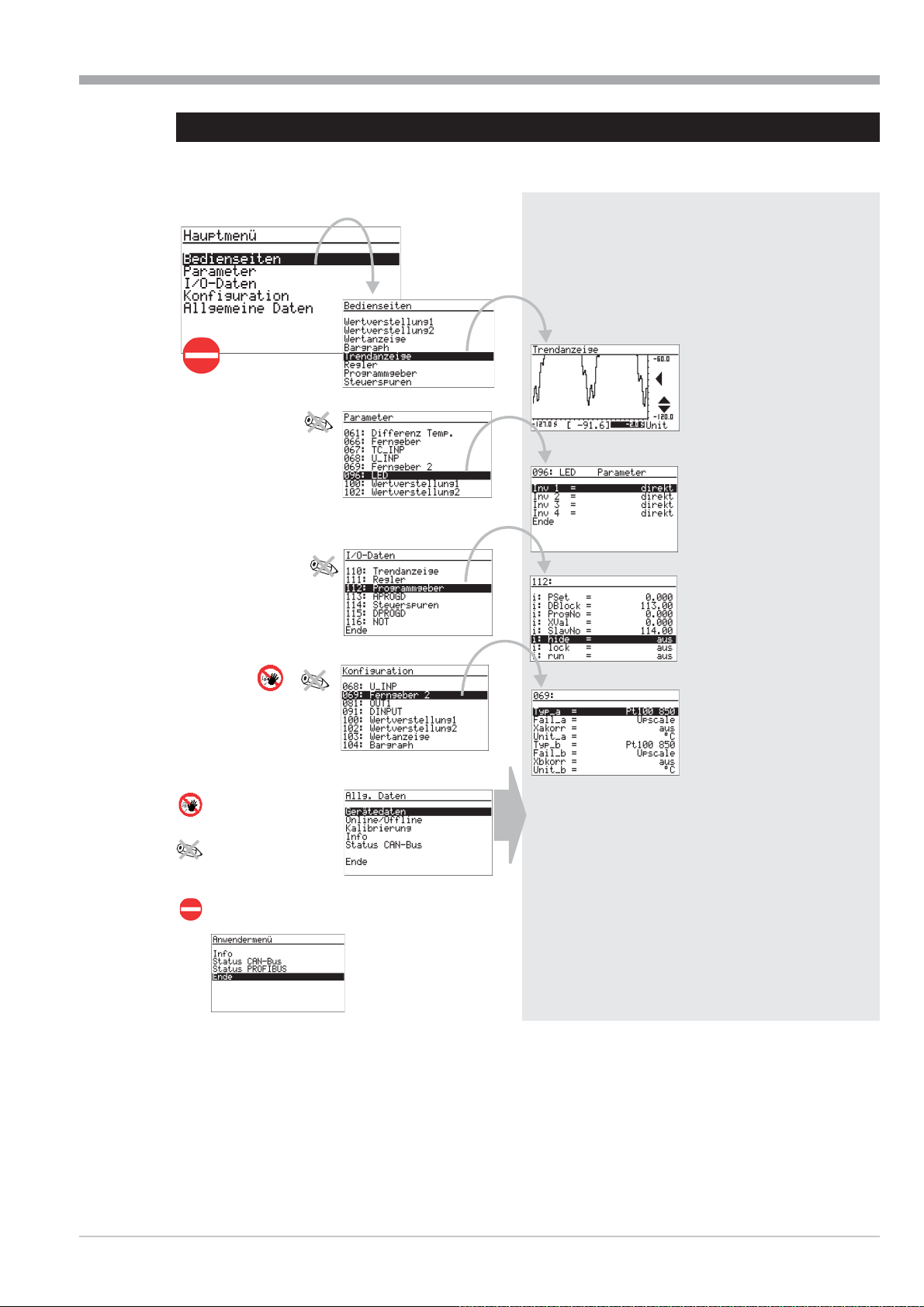
I-8.2 Menu structure

The main menu is the uppermost menu level. Its structure is fixed and independent from the engineering.

Examples:

Dependent on engineering, the operating
pages of the engineering are listed and can
be selected.

List of all functions which
contain parameters.

Configuration disabled

Parameter setting disabled, only
operating pages and Miscellaneous
accessible

If the main menu is disabled, only operating pages
and user menu are accessible.

Kontrast

Programmer

res. transducer2

Date,time: display and setting (only with option B, RS 422)
Device data: interface, mains frequency, language display

and setting (only with option B, TTL/RS422)
Online/Offline: online i offline, configuration cancelling.
Calibration: display and setting of signals to be calibrated
Info: hardware,software order no.,

software release no. display (only with option B, PROFIBUS)
Status PROFIBUS: bus access status, data communication,

available Profibus sharing units (only with option B, PROFIBUS)
Status CANbus: bus access status, data communication,

available CANbus sharing units (only with CAN version)
Status ModC fitted modules and power limit
Contrast: LCD display contrast setting

List of all functions for display of
input/output values

List of all functions which contain
configuration parameters

Fig. 12

Menu structure I-31

Operation 9499-040-82711

I-8.3 Navigation, page selection

+

Operation of the device is by keys M and ID. After pressing key M during 3 seconds, the main menu is always dis
played.

When the main menu is disabled the user menu is displayed.

Fig. 13 Example: Parameters

I

M

D

M

I
D

.
.

M

Procedure

Press ID to select the input field or the line (the selected item is shown inversely).

Ü

Confirm the entry with M (for selecting).

*

.

End

M

I
D

.
.
.

End

-

+

a) If the selected item is a page, the page is opened and navigation can be continued with the ID keys.

Ö

Ö

b) If an input field was selected, the field starts blinking after pressing key M and the required change can be
entered with the ID keys. Confirm with key M. The input field stops blinking and the alteration is saved .

ä

For exit from a page, scroll to menu item “End” at the bottom of the list. When selecting (M), the next higher
menu level is displayed.

Scrolling up is possible.
When exceeding the uppermost menu item, menu item ”End” is displayed.
Unless display of a page is inverse despite actuation of keys ID, the items were disabled (e.g. via engineering.
An inverse menu item which cannot be altered is also disabled.

Operating pages:

These pages offer an additional navigation function:

Continuation or previous pages (marked by an arrow at the

w

bottom (q) or top (p) of the page) can be activated by select
ing and pressing key M.

Items marked with uu open another operating page when

w

selecting (ID) and confirming with key M.

-

+

I-32 Navigation, page selection

Menu item “End” is not provided on operating pages. Scroll until
nothing is selected any more (no input field/line is shown inversely)
and press key M to go to the next higher menu level.

Fig. 14

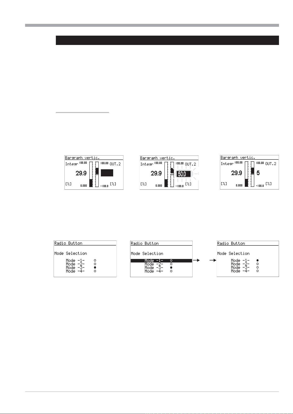
9499-040-82711 Operation

I-8.4 Adjusting values

The menu operating pages include various types of fields for adjustment of values:

- analog values, digital values

- selection lists

- times

- on/off switches

- push-buttons

- selector switches (radio button)

Adjustment procedure

Select the value to be altered with keys ID.

a) Press key M to start value changing (field blinks). Change the value with keys ID.

Press M to store the change (field stops blinking).

Fig. 15 Example: Value adjustment bargraph

I
D

b) The longer keys up/down are pressed, the higher is the acceleration. When releasing, the adjustment speed decrea ­ses accordingly.

Fig. 16 Key H. This mode of adjustment is for switches, push-buttons and selector switches.

50.0

M

I
D

I
D

H

M

46.5

Adjusting values I-33

Instrument settings in the main menu 9499-040-82711

I-9 Instrument settings in the main menu

I-9.1 CAN-Status

The CAN bus status with the connected units is displayed.

Value Signification

1...42

NC
Ck
NR
OK
ES
NA
PO
Er
Op
NU
Wa
Pa
OK

String detemined node name

Node number
NoCheck:
Check:
NoResponse:
Ready:
EMStart:Node has provided an emergency message
NotAvailable: Node status is unknown
PreOperation: Node is in the PreOperational status.
Error:
Operational:
NotUsed: Node is not required by an own
Waiting:
Parametrierung: Lib function just setting the node parameters
Ready:

Node existence not checked so far / node not provided

Node existence just being checked.

No reply from this node, but node is required

Node has replied and is identified

Node is in error status

Node is in Operational status.

lib function.

Lib function waits for identification of this node.

Lib function has finished the parameter setting.

I-9.2 Profibus-Status

The Profibus status page provides information on the Profibus connection
status. The following error statuses are displayed:

•

Bus access not successful

•

Faulty parameter setting

•

Faulty configuration

•

No data communication

I-9.3 ModC-Status

The status page of the modular C card provides information on correct in
stallation. Possible faulty installations are displayed:

•

Difference of configured and fitted module type

•

Power limits exceeded

-

I-34 CAN-Status

9499-040-82711 Instrument settings in the main menu

I-9.4 Calibration

Press ID to select the input and M to open the calibration page.

Transducer input:

Adjusting the transducer start and end:

Select Quit Set transducer to start

Ü

Press MrQuit blinks

*

Press IrSet 0% blinks

Ö

Wait until the input has settled (min. 6 s)

ä

Press Mr0% done is displayed

#

Set transducer to end

<

Press Mr0% done blinks

>

Press I 3x r Set 100% blinks

y

Wait until the input has settled

x

Press Mr100% done is displayed.

c

Calibration is finished. For exit from calibration press D until nothing is marked and then press M.

Transducer

Two resistance thermometers:

Calibration of lead resistance effect

Select Quit .

Ü

Short-circuit both thermometers in the connecting head

Press MrQuit blinks

*

Press IrSet Dif blinks

Ö
ä

Wait until the input has settled (min. 6 s)

#

Press MrCal done is displayed

Lead resistance adjustment is finished. Remove both short cir­cuits. For exit from calibration press D until nothing is marked
and then press M.

I-9.5 Online/Offline

For configuration changing, switch the unit to ‘Offline’ and back to ‘Online’ after alteration.

a

+
+

When switching the unit to status off-line, the outputs will remain in the status at switch-over time !!!

By switching over to on-line, all data is saved.

When terminating the off-line mode by cancellation (Escape config.) the data saved last is loaded back into the wor
king memory.

Temp. difference

-

Calibration I-35

Operating pages 9499-040-82711

#

I-10 Operating pages

The engineering determines the scope of available operating pages. All available pages are listed in the operating
page menu. The various types of pages are explained below.

I-10.1 List display

The operating page list is intended for display/input of process valu
es and parameters.

Apart from digital, analog and time values, values of type radio but
ton, switch and push-button can be defined in the value listing (r
page 33).

The value signification is determined by the engineering. The dis
played values can be input fields.

I-10.2 Bargraph display

The bargraph page is used for display of two analog variables as a bargraph.

Two further variables can be displayed and changed numerically and need not correspond with the bargraph values.

Four further analog inputs can be used to position two markers at the bargraph side, e.g. for indication of the alarm li ­mit or reference values. When exceeding the limits, an arrow q is displayed at the top and bottom end of the bargraph
q (see page 49).

Fig. 17

*

ä

>

y

Ü

Ö

<

x

-

-

Ü
¢

y
¡

-

¥

Ü

Title

*

Name for value

Ö

Unit for value

ä

+¤ Scale end values

<

Display/input field for value

>

Bargraph

y

Bargraph origin

x

Limit value markers for bargraph

I-36 List display

9499-040-82711 Operating pages

I-10.3 Alarm display

Alarm display is in the order of occurrence on a list.

One alarm per line is displayed:

Alarm active alarm text blinks
Alarm active and ackn. Alarm text
Alarm not active any more Alarm text uuu

and not acknowledged

Alarm not active any more --------------------

Acknowledging an alarm

Select an active alarm for acknowledging with ID and acknowledge it with M. New alarms are displayed only
when rebuilding the page, which is done by pressing key H.

I-10.4 Graphic trend curve

The time curve of a process is displayed graphically on the trend page.

Fig. 18

Ü

Title

Ü

+¢ Scale end values

*

*
x

ä
Ö

c

Zoom switchover

ä

Value at time > / actual input value

#
<

Unit of value

>

Origin of time axis related to the actual
value
(=0) shift of time axis (scrolling into the
past)

x

Axis shift signalling

c

End of time axis / earliest value in the
displayed trend

#<>

Zoom value scale

The value axis can be zoomed by factor 1:4 (cut-out magnification).
Select the "zoom" field £, press M, the zoom symbol changes. Now, scaling can be changed by means of keys ID.

The scaling is shifted in steps of 12,5% via field ¢.

Shift of time axis:

Earlier values than those visible in the actual window are also displayed by the trend function (Shift). Values left of
the time axis are earlier values. These values can be displayed by changing the origin of the time axis.

Select field > with ID and shift the scale origin by changing the value.

+

Alarm display I-37

Symbol t (x) indicates the shift.

When resetting the time scale to 0, the shift is switched off.

Operating pages 9499-040-82711

c

I-10.5 Programmer

A programmer controls the process sequence of a plant.

w

Programmers are configurable freely in structure and scope by means of the engineering.

w

A programmer is composed of any number of s (analog values) and control values (digital control bits).

w

Any number of programs (recipes) can be stored for a programmer.

w

The program is divided into a defined number of segments (program segments).

w

The maximum number of segments is determined in the engineering.

w

The maximum scope is defined in the engineering.

w

The actual status of a running program is displayed on the programmer operating page. Dependent on programming,
status (run/stop, auto/manual), segment number, net time and the actual (during manual operation) can be changed.

Programmer operation is divided into:

Program control and monitoring

w

Program (recipe) selection

w

Adjustment of setpoints/control bits during manual operation

w

Parameter setting for program

w

+

Dependent on engineering, parts of this operation can be changed or disabled.

Display of the operating page is always related to one programmer output, whereby analog s and digital control bits
are distinguished. Change to the next programmer output is via field < uu in the title.

Fig. 20

Name of operating page

Ü
* Program name/no. (recipe)
Ö

Ü

*
Ö

ä

#

Fig. 19

Ü

¡

£

¤

<

>

y
x

v

n

m

b

¥

|

x

c
v

[Process value]

ä

Actual segment no.

#

Status line

<

Programmer output switchover

>

/control value

y

Setpoint from...to in the current segment

x

Remaining segment time

c

Elapsed program time

v

Remaining program time

—

Program status
(stop,run,reset,search,program,quit,error)

˜

auto/manual

™

halt, end

n

m

b

Selecting a program

Selection of a program is by alteration of recipe field¡ . Dependent on engineering, selection is from a text list or by
entry of a number.

+

I-38 Programmer

Program selection is possible only in status "reset".

9499-040-82711 Operating pages

Controlling a program

Press key H to control the program sequence:

The time curve can be controlled also by changing the
elapsed time c or segment number £ (preset).

RESET

H

RUN

H

END

H

+

Dependent on engineering, parts of this operation may
be changed or disabled.

Program parameter setting

Select the program for editing via field "Rec" ¡.Callupthe
relevant s/control values, segment times and types with
menu item “program” in the status line (field — ).

A page on which the selected program is displayed as
“RecEdt” is opened. The parameters are listed in the order
of segments.

The data blocks are displayed dependent on engineering.
The type of individual segments can be changed dependent
on data block type.

Selection of all programs including the inactive ones is
possible on line RecEdt in any programmer status.

When using recipe names, these names are displayed on
the editing page. Switching over to the parameters of a dif­ferent recipe can be done by altering the recipe name. This
is possible at any time and does not cause switchover of
the active recipe.

A segment list is completed with end identification

--:-- in parameter Tp
ting the last segment time T
equal to 0), the next parameter is displayed automatically

.=--:-- etc.

T

n+1

This procedure permits shortening of a current program by
adjusting a value<0intherequired position for T

--:-- with key D.

of the last segment. When set

n

to a valid value (higher or

n

=

n

RUN

Fig. 21

STOP

Rec = 1
Wp0 = Wert
Tp1 = Zeit
Wp1 = Wert

Tp2 = Zeit

Wp2 = Wert
Tp3 = Zeit
Wp3 = Wert
Tp4 = Zeit

-

.

.

.

Wpn = Wert
Tpn+1 = --:-­Ende

RESET

scrolling

The following segments will be suppressed in the program.
The relevant segment parameters remain unchanged and
can be re-activated by input of a valid value for T

Programmer I-39

n.

Parameter Step 1

Parameter Step 2

Operating pages 9499-040-82711

p

Segment types

Dependent on segment type, the following parameters can be altered:

Wp i Target setpoint
D i Control value in segment i
Tp i Segment duration
Rt i Segment gradient
Typ i Segment type

Ramp segment (time)

With a ramp segment (time), the runs linearly from the start value (end of previous segment) to
wards the target (Wp) of the relevant segment during time Tp (segment duration).

Ramp segment (gradient)

With a ramp segment (gradient), the runs linearly from the start value (end value of previous seg
ment) towards the target value (Wp) of the relevant segment. The gradient is determined by para
meter Rt.

Hold segment

With a hold segment, the end of the previous segment is output constantly during a defined time
which is determined by parameter Tp.

Step segment

With a step segment, the program goes directly to the value specified in parameter Wp.

The reached due to the step change is kept constant during the time determined in parameter Tp.

-

Wp

T

-

Wp

-

Rt

Tp

Wp

Tp

Waiting and operator call

All segment types can be combined with ”Wait at the end and operator call”.

If a segment with combination ”wait” was configured, the programmer goes to stop mode at the segment end. Now,
the programmer can be restarted by pressing the H-key.

Fig. 22

1 Segment type = Time
2 Segment type = Hold
3 Segment type = Time and wait
4 Segment type = Gradient

1

reset

H

Start Start

START

2

run

PRESET

expired program time

3

stop run

H

4

t

End

control bits 1

control bits 2

program end

END

I-40 Programmer

9499-040-82711 Operating pages

Ü

#

Manual mode

The programmer output can be overwritten for each page.
For this, the relevant page must be switched off to "manual"˜. In this mode, the or control value can be overwritten
>. The control value is changed separately for each control bit. Press M to continue.

Field ˜ permits returning to the automatic mode(r page 38).

+

The program run is not interrupted by the manual mode.

I-10.6 Controller

The controller page permits intervention into process control loops. Input fields (, source, correcting variable during
manual mode, parameter set switchover) are selected via the ID key, pure display fields are skipped.

+

Dependent on engineering, the input fields can be disabled.

Fig.23: Controller operation

*
Ö
ä

<
>

<

>

y

y
>
x

Page title

Ü
*
Ö
ä

#
<
>
y

source (Wint, Wext, W2)

Physical unit

Bargraph of correcting variable Y or XW or

Xeff

Entrance into the self-tuning page

Effective process value

Controller

Value of correcting variable Y or XW or

Xeff

x Self-tuning/command input status
c

Self-tuning result heating

v

Process characteristics heating

—

Self-tuning result cooling

˜

Process characteristics cooling

c
v

b
n

Apart from entries and switchover operations, furt
her actions can be started: Switching over to ma
nual operation is done via key H and field - ¤
provides access to the controller self-tuning page.

Input fields on the operating page

Manual value adjustment

This field can be used to adjust the correcting variable
during manual operation. Adjustment is enabled only du
ring manual operation. Unless manual operation is active,
the field cannot be selected.

When changing over to manual operation, the bargraph
display is always switched over to Y display (correcting
variable), also with X1 or XW defined in the configurati
on. The actual correcting variable is displayed right besi
de the bargraph.

Fig. 24:Correcting variable adjustment via the front panel

-

Temperature

-

-

Manual correcting variable

Alteration of manual correcting variable y by means of keys ID is at three speeds.

Press the key to start the adjustment at a speed of 1% / sec. After 3 sec., switchover to 2.5% / sec occurs and switchover to
10%/sec. is after another 3 sec.

-

-

Y

Controller I-41

Operating pages 9499-040-82711

The internal can be altered at any time,
also when another is active.

source

source switchover is possible via a selection field on the

controller page.

Dependent on controller configuration, selection of Wint,
Wext and W2 is possible.
The field can be left with Quit, if no switchover is needed,

Fig.25 : adjustment via the front panel

Temperature

W

Fig. 26 Front-panel switchover

Temperature

Wsource

Self tuning

Determination of the optimum process parameters is possible by self-tuning. Self-tuning is available for processes
with compensation and no delay time.

Dependent on controller type, parameters Xp1, Xp2, T

, Tv, Tp1, Tp2 are determined.

n

+

Preparation

Adjust the desired controller behaviour.

w

e=0.0.

w

P- controller: Tn = 0.0 Tv = 0.0

w

PD- controller: Tn = 0.0 Tv > 0.0
PI- controller: Tn > 0.0 Tv = 0.0
PID- controller: Tn > 0.0 Tv > 0.0

If a controller has several parameter sets, selection of the parameter sets to be optimized is required

w

(( POpt=1...6). If necessary, these settings must be made available when creating the engineering ).

Switch the controller to manual mode (key H). Alter the correcting variable to reach the working point.

w

The process must be in a stable condition. Self-tuning starts only, when process value oscillations are smaller than

0.5% of the control range during one minute (controller display:‚ process at rest’ (PiR)).

If necessary, other control loops in the plant must be set to manual mode as well.

Fig. 27 Calling up the self-tuning page

I-42 Controller

9499-040-82711 Operating pages

+

reserve:

To permit self-tuning, the distance between setpoint and process value must be higher than 10% of the setpoint range
before self-tuning start.

With inverse controllers, the must be higher than the process value. With direct controllers, it must be smaller.
The determines a limit which is not exceeded during self-tuning.

!

Self-tuning start

Select function Stat: OFF/OK and con
firm it with M. Stat:OFF/OK blinks and
is switched over to Stat: Start by pres
sing I.

Fig.: 26 Self-tuning with heating and cooling

-

X, W

-

60s

PiR

W

I

> 10% W0/W100

X

Pressing key M starts the self-tuning attempt.
The can be changed also subsequently. After
successful self-tuning, the controller changes to
automatic operation and controls the with the
new parameters.

When ‘Process at rest’ (PiR) is detected and a
sufficient reserve is provided, the correcting va

Y

100%

+

0%

-

Off/Ok

+

Start

H

dYopt

PIR_H

Start

Adaption

Step Off/Ok

Optimisation

finished

t

t

riable is changed by output step (increased with indirect controller, decreased with direct controller).

The size of the output step change is set to 100% as standard. In critical processes, this value (parameter dYopt) may
have to be reduced to prevent damage to the process. The parameter is adjustable in the engineering, or via the para ­meter dialogue of the main menu, if the engineering is known . In case of doubt, contact the programming engineer.

When self-tuning is finished with an error (Ada_Err or 0err on the controller page), the initial correcting varia­ble is output until self-tuning is finished by pressing key H.

a

Self-tuning procedure with heating and cooling processes:

(3-point / split-range controller)

Self-tuning starts as with a “heating” process.

After self-tuning end, the controller settings
based on the calculated parameters are made.
This is followed by line-out at the pre-defined ,
until PiR is reached again.

Subsequently, a step to cooling is made to de
termine the “cooling” parameters. When can
celling the cooling attempt, the parameters for
“heating” are also taken over for cooling. No
error message (Ada_Err) is output.

Whilst self-tuning is active, the control function is switched off!

Fig.29:

X

W

Y

100%

-

-

-100%

Off/Ok

YOptm

0%

Start

+

PIR_H

60s

PiR

60s

Optimization

Start

Adaption

heating

ready

Step Off/Ok

PiR

dYopt

PIR_K

Optimization

cooling

ready

Step

t

t

Controller I-43

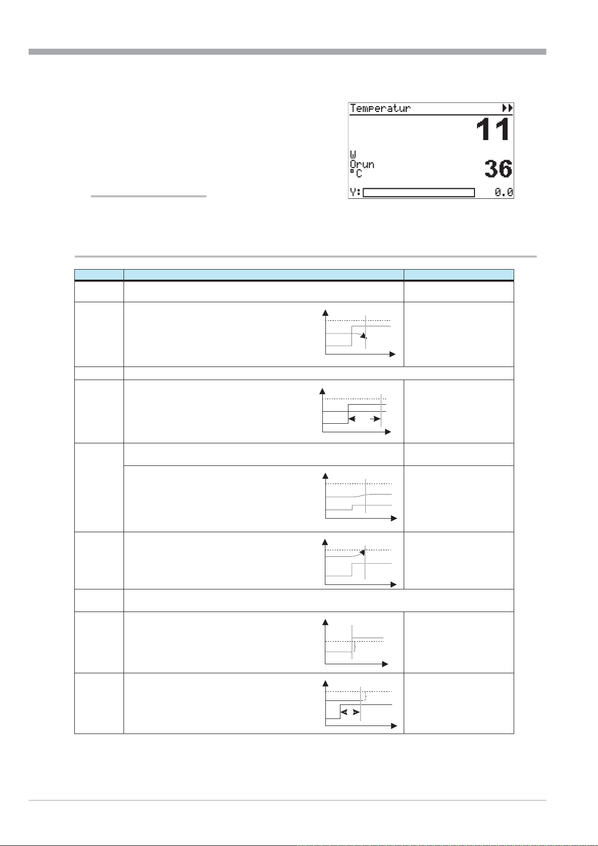
Operating pages 9499-040-82711

X

X

t

The self-tuning statuses are indicated with priority in
the display field for manual operation.

Self-tuning running, display: ORun

w

Self-tuning faulty, display: OErr

w

Fig.30: Controller page with started self tuning

Self-tuning completed with an error is finished by
pressing key H twice.

Self-tuning cancelation

Self-tuning can be stopped at any time by pressing key
H, or by selecting Stop in the Stat field (status).

Signification of self-tuning messages ORes1/ORes2 for controller type CONTR and CONTR+

ORes1/2 Signification or trouble cause Possible solution

0

1

2
3

4

No attempt was made or attempt cancelled by Stat: Stop or
switchover to manual mode ( H key) .

Cancellation:

Faulty correcting variable output action,

W

Cancellation

Change controller
output action.

X does not change in the direction of W.

Y

t

Finished: self-tuning was completed successfully (reversal point found, safe estimation)
Cancellation:

The process does not respond or responds too

W

Cancellation

Close control loop.

slowly (change of {X smaller than 1% in 1 hour)

>1 Std.

Cancellation

t

Optimum result with low re­versal point

Increase output step change
dYopt.

Completed, withou6 AdaErr:
Successful attempt, process has a low reversal point

Cancellation, with AdaErr:
Attempt failed, process stimulation low
(Reversal point found, but estimatio n is unsafe

Y

W

X

Y

5

6

Cancellation:

Self-tuning cancelled because of exceeded

hazard.

W
X

Y

Cancellation

Completed: attempt successful, but self-tuning cancelled due to exceeded hazard.

Increase separation of pro
cess value (X) and (W) when
starting, or decrease

YOptm .

(Reversal point not reached so far; safe estimation).

7

Cancellation:

Cancellation

Output step change too small, {Y < 5%.

Ymax

Y

8

I-44 Controller

Cancellation:

reserve too small, or exceeded

whilst PiR monitoring is busy.

W
X

Y

{Y<5%

Cancellation

<10% W0..W100

>1 Std.

Increase Ymax or set
Yoptm to a smaller value.

t

Vary stable correcting vari
able YOptm.

t

-

-

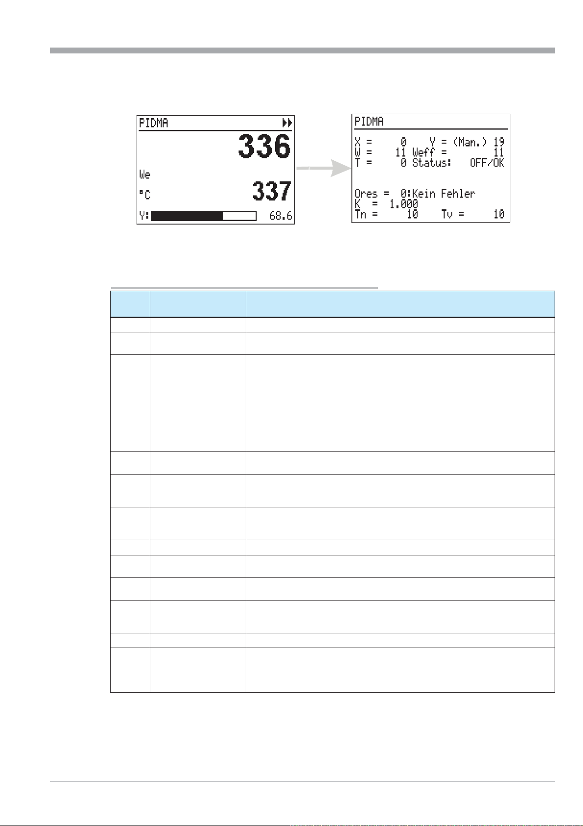
9499-040-82711 Operating pages

The controller type PIDMA offers the following self-tuning page.

Fig. 31 Optimization page

For self-tuning preparation, parameters must be adjusted dependent on process and engineering. For this purpose, spe
cial knowledge of the applicable function block is required, i.e. it should be done by the programming engineer. Self-tu
ning start is as described above.

Signification of self-tuning messages ORes for PIDMA

ORes

0
1

2

3

4

5

6

7
8

9

10

11
12

Signification or
error cause

No attempt was made

Xlimit too small Step change threshold too small: compared to the process noise, the step change thresh

dYopt large Positioning pulse too high: the correcting variable would exceed the positioning limits

Start again No rest. The autotuner has detected that the process is probably not at rest. Please wait,

dYopt small Positioning pulse too small: the step response is hidden by process noise. Start a new at-

No peak Max. detection failed: after output of the positioning pulse, no maximum / minimum in

Output sat Positioning limits during self-tuning were exceeded. During the attempt, correcting vari

Controller type No self-tuning result for the specified combination P/I/D can be found.

Monotony Process not monotonous: the process has a strong all-pass behaviour ( temporarily, the

Extrapolation Extrapolation failed: after the positioning pulse end, no process value decrease was de

Bad result Result useless: excessive noise, or the determined process parameters do not correspond

Man. break The self-tuning attempt was canceled manually by the operator with „STOP“.

Direction Faulty output action: the expected output action of the step response is opposed to the

Possible solution

old is too small. Start a new attempt with a higher positioning pulse.

when the selected pulse height is output. Start a new attempt with smaller positioning
pulse or reduce the correcting variable in manual mode previously.

until reaching the rest condition. Another possibility is to activate the drift compensation

or to increase the positioning pulse. Note: With pulse width modulated (PWM) control
outputs (2 and 3-point controller), oscillations of process value PV are susceptible to occur
even during manual mode, if the corresponding cycle time t1 (t2) is too long. In this case,
the controller cycle times should be as low as possible.

tempt with a higher positioning pulse, or take measures to reduce the noise (e.g. filter).

the process value curve was detected. The settings for the process type ( with / without

compensation) should be checked.

able MV has exceeded the positioning limits. Repeat the attempt using a smaller posi

tioning pulse or a reduced correcting variable during manual mode.

process value runs in opposite direction ) or serious trouble during the attempt.

tected because of excessive noise. Increase the positioning pulse or attenuate the noise.

to the description of a process with dead band. Start a new attempt with a higher posi

tioning pulse or attenuate the noise.

correcting variable.

Cause can be faulty setting of the output action, or e.g. inverting actuators. Change the

controller output action.

-

-

-

-

-

-

-

Controller I-45

Operating pages 9499-040-82711

c

I-10.7 Cascade controller

+

With cascade control, two coupled controllers act on a common actuator. A process value for the master and a pro
cess value for the slave controller are required.

ambient temperature pre travel temperature

The slave is determined via the external by the master. Cascade operation is possible in the following statuses:

Automatic mode

In a cascade, master and slave operate automatically during automatic mode. The master and process value are the
relevant variables for process control. The master is adjustable. The process value of the slave
tionally.

"Cascade" is displayed.

¨ is displayed addi

-

-

Operating page title

Ü
* Parameter set selection, if available
Ö

Switchover field cascade mode (open/clo­sed)

ä
#

<
>
y
x
c

v

—

source of master (W

Display field for manual mode (otherwise
empty)

Physical unit (master block parameter)
Entry into self-tuning
Master process value
Slave process value

(from master in automatic mode, from sla

ve with open cascade)
Bargraph and display

(Y from slave or X/XW from master)
Display of slave selection with open casca
de (otherwise empty)

int,Wext,W2

)

Fig. 32 Operating page of a cascade controller in automatic

Ü

*

Ö

ä

#

<

-

-

b

>

y

x

v

I-46 Cascade controller

9499-040-82711 Operating pages

Cascade opened

For opening the cascade and control by means of the slave controller (see note text “Slave” on the operating page),
switchover field ¢ is switched to “Casc- Open”.

+

+

"Casc-open" is displayed.

The slave is displayed now.

Now, the slave controller becomes the variable
used for process control and can be adjusted.

The process value of the master control loop is
set by the cascade loop rather than being con
trolled. Switchover between operation by mas
ter or slave is always possible.

In cascade mode, the master information is dis
played in the fields for , source, physical unit
and X/XW bargraph. With open cascade (display "Slave"), the slave information is displayed.

Manual mode

Switchover to manual is via key H (display in field¤). The cascade status (open/closed) is not affected. In manual
mode the process is controlled directly with the slave correcting variable. The slave correcting variable can be adjusted
during manual operation.

"Man" is displayed.

Fig. 33 Cascade controller with open cascade

-

-

-

+

Cascade optimization

In a cascade, the slave controller and then the mas­ter must be optimized.

The self-tuning entry of the cascade operating page
uu relates always to the slave!

For optimizing the master controller, the master
must be selected purposefully via the operating
menu. For this, the project description must be used.

Fig. 34 Cascade controller in manual mode

Cascade controller I-47

Maintenance, test, trouble shooting 9499-040-82711

I-11 Maintenance, test, trouble shooting

I-11.1 Cleaning

Housing and front panel can be cleaned using a dry, lint-free cloth. No use of solvents or cleansing agents!

+

Avoid using solvents or cleansing agents!

I-11.2 Behaviour in case of trouble

The unit needs no maintenance. In case of trouble, check:

Is the unit in on-line mode ?

w

Is the supply voltage connected correctly? Are voltage and frequency within the tolerances?

w

Were all connections made correctly ?

w

Do the sensors and actuators work properly?

w

Is the engineering OK?

w

Is the unit configured for the required operating principle?

w

Do the adjusted parameters have the required effect?

w

Are the I/O extension modules plugged in and clicked in position correctly (modular option C)?

w

Is a terminating resistor activated (can be required dependent on the instrument position in the bus topology with

w

CANopen and PROFIBUS DP)?

Were the required EMC measures carried out (screened cables, earthings, protective circuits, etc.)?

w

Does the diagnostic page of the test engineering indicate an error?

w

If the unit does not function correctly after these checks, it must be shut down and replaced. A defective unit can be
returned to the supplier for repair.

I-11.3 Shut-down

a

Disconnect the supply voltage completely and protect the unit against accidental operation. As the instru ­ment is mostly connected with other facilities in the control loop, consider the effects before switching
off and take measures to prevent the occurrence of undesired operating conditions!

I-11.4 Test engineering as basic equipment

KS98-1 is factory set for a test engineering IO-test.edg, which ensures checking of the possible inputs and outputs of
the extended basic unit (standard + option B + option C). If KS98-1 is provided with a customer-specific engineering,
the relevant description is applicable.

!

If KS98-1 is provided with customer-specific engineering, the engineering description is applicable.

A diagnostic page is provided to indicate system errors in case of start-up problems. The availability of the real-time
clock is also displayed. The display colour can be changed green/red and normal/inverse.

I-48 Cleaning

9499-040-82711 Maintenance, test, trouble shooting

Fig. 35 Menustructure of the test-engineering

Test engineering as basic equipment I-49

Maintenance, test, trouble shooting 9499-040-82711

I-11.5 I/O-Test

Input and output type and measuring/signal range are configurable.
For this, switch the unit to OFFLINE(r page 35) first after starting up. All inputs and outputs are preset to 0 .. 20mA

and 0-100% value range.

Before commissioning, the inputs and outputs to be connected must be configured for the required sensor type via
main menu “Configuration”.

+

After adjusting the correct type, the unit must be switched back to ONLINE!

Now, KS98-1 is ready for the first input/output test.

Possible settings:

AINP1: thermocouple types; Pt100; 2*Pt100; 0/4 .. 20mA; 0/2 .. 10V; transducer 500W; resistance 500W 250W

w

AINP3 (option C): 0/4 .. 20mA

w

AINP4 (option C): 0/4 .. 20mA

w

AINP5 : 0/4 .. 20mA

w

AINP6 : 0/4 .. 20mA

w

OUT1 : 0/4 .. 20mA or relay

w

OUT2 : 0/4 .. 20mA or relay

w

OUT3 (option C) : 0/4 .. 20mA

w

OUT4 : relay

w

OUT5 : relay

w

Dependent on instrument selection, outputs OUT1 and OUT2 can be relay or current output. Accordingly, they must be
controlled digitally or analoguely in the engineering.

As all outputs were defined as analog outputs in the present engineering, a value below 50% (corresponds to logic
“0”) and a value above 50% (corresponds to logic “1”) must be set for relay output testing.

Outputs OUT4 and OUT5 are always relays, i.e. they are controlled digitally on the relevant operating page. (Adjusting
values r Navigation page 32).

Adjusting the output values and selecting the pages are done as described. Continuation pages are selected using
keys ID via the menu lines ( p, q) and called up with M.

This engineering is not suitable for controlling a plant. For this purpose, a customer-specific engineering is required
(see versions, section: Adjustment on page 18).

a

I-50 I/O-Test

Faulty settings can cause damage to instrument and plant!

9499-040-82711 Survey

II Engineering-Tool

II-1 Survey

The engineering tool for KS 98-1 enables the user to make an engineering which is specially tailored for his applicati
on. The engineering tool mainly comprises a function block editor supported by the IEC 1131-3 standards.

The engineering tool offers the following functions:

By selection from a menu, functions can be selected and placed in the working window.

w

Outputs and inputs can be connected graphically.

w

When shifting functions, the connections are dragged.

w

Function configuration and parameter setting.

w

Downloading of the engineering into KS 98-1.

w

Adjustment management.

w

Long-term storage of various engineerings on hard disk or floppy.

w

Coupling the PC with the KS 98-1 multifunction unit is done via an RS232/TTL adaptor cable, which can be ordered se
parately ( order number : 9407 998 00001).

II-1.1 Scope of delivery

The engineering tool scope of delivery comprises the following components:

One CD-ROM for English, French, and German version.

w

the operating instructions

w

licence conditions

w

registration with licence number

w

-

-

Scope of delivery II-51

Installation 9499-040-82711

II-2 Installation

II-2.1 Hardware and software prerequisites

For using the engineering tool, the following system prerequistes must be met:

min. 486 IBM-compatible PC,

w

at least 8 MB working memory

w

VGA card and suitable monitor (min. screen resolution 800 * 600 pixels)

w

hard disk with min. 2,5 MB free memory

w

Diskette drive / CD drive (CD-ROM can be copied onto diskettes)

w

MS-Windows from version 3.1

w

(tested: Windows 3.1, Windows for Workgroups 3.11 and Windows 95)

a free serial interface (COM1 - COM4)

w

mouse required, adjustment as a double-key mouse in standard mode for right-handed operators

w

II-2.2 Software installation

Installation from CD

Place the CD into the CD drive and select the relevant path to install the required software. The CD drive is assumed to
be drive “D” in the example below.

To install ET 98: D:\install\ET98\cd\Setup.exe
To install ET 98plus: D:\install\ET98plus\cd\Setup.exe
To update ET 98: D:\install\ET98plus.UPD\cd\Setup.exe
To upgrade ET 98plus: D:\install\ET98plus.UPG\cd\Setup.exe

Installation from diskette

Generating the installation diskettes.

The software is supplied on a CD-ROM. Installation diskettes can be generated simply by copying the corresponding
folders from the CD to diskettes.

The CD drive is assumed to be drive “D” in the example below.

Generating ET 98 diskettes:

Copy the complete contents of D:\install\ET98\disk1 to ...\disk4 onto four diskettes.

Generating ET 98plus diskettes:

Copy the complete contents of D:\install\ET98plus\disk1 to ...\disk6 onto six diskettes.

Generating an ET 98 update diskette:

Copy the complete contents of D:\install\ET98plus.UPD\disk1 onto a diskette.

Generating ET 98plus upgrade diskettes:

Copy the complete contents of D:\install\ET98plus.UPG\disk1 to ...\disk6 onto six diskettes.

Installation: Place the first diskette into the drive. Click on “Start” (or open Program Manager) and select “Execute…”
(open “File”). Enter ”A:SETUP” (or ”B:SETUP” if your diskette drive is “B:”), and follow the instructions on the screen.
Depending on the language you are working with, not all diskettes might be needed.

II-52 Hardware and software prerequisites

9499-040-82711 Installation

II-2.3 Licencing

During initial installation of the engineering tool,
an input mask (r Fig.:36 ) for entry of the licence number is dis
played. Unless a licence number is entered, the engineering tool
starts only as a demonstration version with limited functions (sa
ving and downloading of an engineering into KS 98-1 is not pos
sible in the demonstration version). The licence number is given
on the enclosed registration form. Please, keep the registration
form carefully. You need the licence number in case of re-instal
lation and when you have to make use of the technical support.
Please, complete the registration sheet immediately and send it
to the specified address via fax or as a copy via mail. In return,
you will get technical support and regular information on product
updates.

Please, note the PMA licence conditions for software products. Successful installations
are only possible onto a hard disk, but not on a network drive (only on request).

Fig.: 36

-

-

-

-

Fig.: 37

Updates

The licence number is stored in the system and need not be re-entered in case of an update.

Changing the licence number

A change of the licence number or licensing of a demonstration ver­sion (conversion into a full version) can be done via the menu bar
(r Fig.:37 )“Lizenz”. In the window (r Fig.:38 ) displayed after cli­cking on Licence, input mask ‘PMA licensing’ (r Fig.:36) can be
called up via Edit. Now, the new licence number can be entered in
this input mask.

II-2.4 Software start

Starting software “engineering tool KS 98-1" is by double-clicking on the icon created by the installation program in
program group ”PMA Tools".

Fig.: 38

Licencing II-53

Menu reference to the engineering tool 9499-040-82711

II-3 Menu reference to the engineering tool

II-3.1 Menu ‘File’

This menu item permits standard data
handling functions which are also known
from other Windows programs (r see
Fig.: 39). Via this menu, e.g. finishing the
program is possible.

New

Select command “New...” in the file menu, if you want to open an empty engineering without title. Working width /
height and scroll bars are set to standard values. The existing engineering is removed from the working memory.

Fig.: 39

Open

This function can be used for reading in already created
engineerings. After selection of this command, a standard
dialogue box (r Fig.: 40) in which the relevant drive as
well as the required path and file name are selected is
displayed.

Via drop-down list “File format”, adjustment which kinds
of files are displayed in the file list is possible.

After confirmation with OK, the file is loaded.

This command can be used for loading a stored enginee
ring for editing. If write-protected is selected, a new name is always required when saving (Save as).

Fig.: 40

-

Save

This function can be used for saving an engineering created by you as a file. Storage is with the file name used when
reading in. If no name exists (new Engineering), select the required path, enter a valid name (with omission of the file
extenstion, standard extension .EDG is used automatically) and acknowledge with OK. If there is already a file with the
same name, a message is displayed. When saving this file repeatedly during an operation, re-selection of this menu
item is sufficient, whereby the name need not be entered repeatedly.

Save as

This function permits saving of an already loaded project under a different name. For this, enter a new name into the
field provided for this purpose. If the file extension is omitted, the file is saved automatically with extension .EDG.

II-54 Menu ‘File’

9499-040-82711 Menu reference to the engineering tool

Project info

Execution of this command is followed by display of an input mask for specification of general information on the pro
ject. Date of modification and operating version are entered automatically.

The following parts of the project info are stored in KS 98-1:

the first line ‘Project name‘ (max. 45 characters can be edited freely) the modification data and the operating version

Fig. 41

After clicking on button a window for text entry for the drawing header is opened (r Fig.:42).

Fig.: 42

-

For print-out with drawing header, tick box ‘Use frame’ (r see g Fig.:42).

Fig.: 43 Frame header

(Modifying the frame header; see also the section “Print r Graphic print-out with frame header”)

Menu ‘File’ II-55

Menu reference to the engineering tool 9499-040-82711

Project PC t KS 98-1

After calling up this menu item, an additional selection
(see Fig. 44) is displayed.

Engineering

Complete engineering read-in.

Para/Config

Configuration and parameter data read-in. To ensure correct data read-in, the engineering in the instrument and in the
engineering tool must be equal.

Function block

Configuration and parameter data read-in of a function block marked in the engineering.

Fig.: 44

+

+

With password protection of an engineering, dialog box “Log in” (see Fig.: 45) is displayed. This dialog box asks you to
enter the password for the existing engineering.

Fig.: 45

Exceeding the “number of permitted faulty attempts” (see Fig.: 51)
deletes the engineering in the multi-function unit

Project PC r KS 98-1

Function block
Transmission of configuration and parameter data of a function block
marked in the engineering.

After calling up this menu item, an additional selection is displayed
(r Fig.: 46).

Engineering

After selecting this menu item, a dialogue box is displayed

(r Fig.:32 ).

When clicking on the OK button, the actual engineering is transmit

ted into KS 98-1 without password protection.

Fig.: 46

Fig.: 47

-

The project stored in the instrument so far is overwritten. The possible messages are shown below.

Fig.: 48 Fig.: 49 Fig.: 50

II-56 Menu ‘File’

9499-040-82711 Menu reference to the engineering tool

When clicking on button “new password” in the dialogue

Fig.: 51

box, the password dialogue is opened (see Fig.: 51).

Enter password, password mode and number of permitted
faulty attempts.

When clicking on button OK, the current engineering is
transmitted into KS 98-1 with password protection.

Thereby, the project stored in the unit so far is overwrit

-

ten.

The message shown in Fig.:51 indicates an error in the transmitted data and is used for trouble shooting in case of
technical questions.
The password mode determines the access privilege (? see following table) to the KS 98-1 data via the interface.

Export

After calling this instruction,
you must define whether the
parameters and configuration
data of the individual function
blocks (text file r see Fig.:

52), the graphical engineering
(graphics in .wmf format) or the variables list are to be exported.

Fig.: 52

Print

After calling up this menu
item, an additional selection is
displayed (r Fig.:53 ).

Graphics

Engineering print-out

Text

Print-out of parameter and configuration data of
individual function blocks (text output r see
Fig.:54 )

Connecting diagram

Print-out of the connecting diagram (see page55 for
connecting diagram)

Subsequently, the standard mask for adjusting prin
ter functions under Windows is displayed. The pos
sible settings are described in detail in the
Windows documentation.

The data of the actual project are output in a standard form on the connected printer. The current standard printer ad
justed under Windows with standard font is used for this purpose (MS Sans Serif 2,8mm).

Fig.: 53

Print

Fig.: 54

======================================================
Blocknummer:101 Funktion : Analoger Programmgeber
Abtastzeitscheibe=11

------------------------------------------------------

......................................................

......................................................

Short-Parameter =3

WMode = 0
PMode = 1
TPrio = 0

Float-Parameter =1

-

-

Wp 0 = 0.000000

Short-Konfigurationen =3

PwrUp = 2
PEnd = 0

Turbo = 0
Float-Konfigurationen =0
Text Parameter =1

Text 1= APROG

Graphics
Text
Connecting diagram

-

Menu ‘File’ II-57

Menu reference to the engineering tool 9499-040-82711

Print-out of a section

For printing parts of an engineering, the part to be printed
must be marked in the survey mode. In the standard prin

Fig.: 55

­ter mask (see Fig.:55 ), click on “Mark” (“Mark” with
Windows 95) before starting the print-out. This is only
possible with graphic print-out. Printing out a section with
drawing header is not

possible.

Graphic print-out with frame header

Graphic print-out is possible with or without frame hea
der. As standard, printing is without frame header. Selec

-

-

tion is in input mask ‘Drawing header’ (r p. 55 Fig.: 42)

In the drawing header, additional information such as operator, date, version no. etc. can be entered. On the left besi
de the PMA logo, there is free space for a customer-specific logo. The PMA logo can be removed or replaced by a
customer-specific logo.

The frame header is in .wmf format (in ...\PMATools\Et98.xxx\Framexd.wmf) and can be edited with normal graphic pro
grams(e.g. CorelDraw). However, fields and frames should not be changed to prevent faulty positioning of the texts en
tered in the engineering tool.

-

-

-

II-58 Menu ‘File’

9499-040-82711 Menu reference to the engineering tool

Page grid in the engineering survey

An engineering can be printed out either completely on only one page, or as a marked section.
By mouse-clicking (left key) in any position of the engineering with key pressed, a page grid on which the engi
neering can be printed out is included into the survey (r Fig.:56). The pages are numbered linewisely from left to right
and from top to bottom in the print-out and can be printed out with or without frame header. Pagewise print-out is pre
pared by ticking ‘pages’ in the standard printer mask (see Fig.:55 ) Pressing key + clicking with the mouse in
the top corner of the survey removes the grid.

In the normal view, the page borders are shown as broken lines.

Fig.: 56 Setting up a page grid

-

-

C:\PMATOOLS\ET98.20D\PRJ\xx.edg (last 4 projects)

The last 4 handled or stored projects are displayed. The project is loaded after clicking on it.

Exit

This command finishes working with the engineering tool. Moreover, finishing the program via the system menu field
is possible, as in every Windows-supported program. For this, select option “Exit” accordingly. Before finishing, you
may be asked, if you want to save the changes in the project handled last. If you deny, the changes are canceled, ot
herwise, they are stored. Select “Cancel”, or press key “ESC” for exit from the dialogue box and returning to the
current project.

-

Menu ‘File’ II-59

Menu reference to the engineering tool 9499-040-82711

II-3.2 Menu ‘Edit’

Timing

This command calls up the timing dialogue in the normal view. This dialogue can be used for determination of the time
slot assignment for each function block. Time slot assignment can be done also from the parameter dialogue
(r Fig.: 59). In the survey, a handling simulation which indicates the order in which the function blocks are calculated
is called up.

The timing dialogue shall indicate the time consumed by the
function blocks in the time slots, as well as the handling sequen
ce. Therefore, two different time slot selection functions are avai
lable. The timing sequence is displayed in the bottommost line,
whilst the individual time slots are displayed at the top. If a scan
ning time of a time time slot is selected, all function blocks which
are calculated in this time slot part are displayed in the left box.
Thereby, the order corresponds to the timing sequence.

The right box contains all function blocks which are not allocated
to a time slot so far.

If a function block is selected, it can be shifted into this time slot
by mouse clicking on the relevant field. Clicking outside a time
slot will remove it from a time group without re-allocating it.

If several function blocks are to be moved simultaneously, they
can be selected by means of or with the left mouse key. As default, the engineering tool assigns the newly placed
function blocks to the time slot with 100 ms scanning time. The total of
calculation times of all function blocks per time slot must not exceed 100%.
A calculation time of a time slot exceeding 100% is displayed by a colour
change (red) in the timing dialogue (see Fig.:58 ).

In this case, the function block repartition must be changed.

The survey display shows a simulation that indicates in which sequence the function blocks are calcu­lated. The sequence is either shown automatically, or is defined individually by the user via the keys v
(= forwards) and r (= backwards).

Fig.: 57

-

-

-

Fig.: 58

II-60 Menu ‘Edit’

9499-040-82711 Menu reference to the engineering tool

Parameters

This command can be used for calling up the parame
ter dialogue of a selected function (r Fig.: 59). Its
function is equivalent to clicking with the right mouse
key with the function marked. In the parameter dialo
gue, the parameter and configuration data of the
function blocks are adjusted. With parameter or confi
guration data with which the required setting can be
selected from a text group, an additional dialogue in
which the possible settings are offered via a
drop-down item is called up Ü at the moment at
which the text is changed. A help text concerning the
relevant parameter is displayed in a frame Ö .

Moreover, the block number and the time group allo
cation (scanning time code *) can be changed, if
necessary. The block number determines the handling
sequence within a time slot. The block number can be
changed into any value required for this function. Nor
mal calculating functions can be set to block numbers ranging within 100 and 450. If the new block number is already
used, all other functions are shifted upwards by one, until a free block number is reached. Unless a free block number
can be found, allocation of block numbers is refused

Fig.: 59

-

-

-

-

-

Delete

Deletes the marked function or connection (Del key)

Wiring / Positioning

Toggles between the wiring and the placement mode. Switching over can be done also by double-clicking with the left
mouse key.

In the wiring mode, connections can be created, changed and deleted.
The placement mode permits function placement, shifting and parameter setting.

Standard connection

A connection which was changed manually can be re-calculated automatically via this command.

Survey (Key ‘a’)

Display of the overall engineering or switch-over to normal view (wiring mode).When clicking in the survey with the
right mouse key, the engineering tool changes to the clicked position in the normal view. An area marked in the survey
can be printed out selectively (see page 58).

Add text

If this instruction is called, a
window is opened, in which a
single-line text block with max. 78
characters can be entered (see
Fig.: 60). This text serves as a
brief explanation at any point in
the engineering. The text can be
moved and deleted like any other
block.

Fig. 60

Menu ‘Edit’ II-61

Menu reference to the engineering tool 9499-040-82711

Reorg Block No.

Subsequent deletion of functions produces “gaps” in the list of as
signed block numbers. The menu item “Reorg Block No.” opens a
dialog box (see Fig.:61 ).

After confirmation with “OK”, all the block numbers are renumbe
red consecutively. If the default value “0" of the parameter ”Free
block numbers" is changed (e.g. =10), all block numbers are increa
sed by the specified value, and free spaces are eliminated.

-

-

-

Fig.:61

Search

Selecting this menu item opens the
window “Search function” (see
Fig.: 62).

It is possible to search for existing
elements in the different groups.

All possible items are displayed in
a list box, where they can be selec
ted. If the search is successful, the
corresponding part of the enginee
ring is displayed, whereby the iden­tified element appears inverse.
Fig.:62 shows examples of block
names.

Fig.:62

-

-

Enlarge sheet

With a very extensive engineering, increasing the window greater may be necessary.

Move

Shifts the overall engineering horizontally and vertically.

The x value shifts in horizontal and the y value shifts in vertical direction. Negative values shift left or up. A value of
100 shifts by approx. the size of a small function block.

Add

This command can be used for ad
ding saved engineerings, inclusive of
all adjusted parameters, to the one
loaded instantaneously. Unless furt
her block number ranges for defined
functions are free in the current engi
neering, an error message
(r see Fig.:63 ) is displayed.

Recurrent individual parts can be composed quickly into new engineerings by saving them (e.g. programmer, control
lers with particular parameter settings, etc.)

-

Fig.: 63

-

-

Undo (Ctrl + Z)

-

This command can be used for canceling the last action.

II-62 Menu ‘Edit’

9499-040-82711 Menu reference to the engineering tool

II-3.3 Menu ‘Functions’

Menu ‘Funktionen’ permits selection of all KS 98-1 software
functions with variable block number. After clicking on
‘Functions’, a list of the functions classified in groups is dis
played. When clicking on a function group (e.g. scaling and
computing 2) the software functions belonging to this group
are displayed as block diagrams
(r Fig.:64). Click on a block diagram to select this function.
The selected function is displayed in the bottom left status
field and remains selected, until it is replaced by another
function.

Selection of a function existing in the engineering selects this
function for positioning.

Clicking with the right mouse key places the selected function
in the mouse pointer position.

Further functions can be selected under menu ‘Fixed funct.’.

Depending on the selected operating version, the displayed
functions can vary.

II-3.4 Menu ‘Fixed funct.’

Menu ‘Fixed functions’ permits selection of all KS
98-1 software function with fixed block number.
After clicking on ‘Fixed functions’, a list of the
functions classified in groups is displayed. When
clicking on a function group (e.g. Digital I/O) the
software functions belonging to this group are dis­played as block diagrams
(r Fig.: 65). This function is selected by clicking
on a block diagram. The selected function is dis­played in the bottom left status field and remains
selected, until it is replaced by another function.

Clicking with the right mouse key places the selec
ted function in the mouse pointer position.

Fixed functions can always be selected only once.
These functions are e.g. for inputs or outputs, or
status functions. All these functions are sorted au
tomatically in the block number range below 100.

Fig.: 64

-

Fig.: 65

-

-

Menu ‘Functions’ II-63

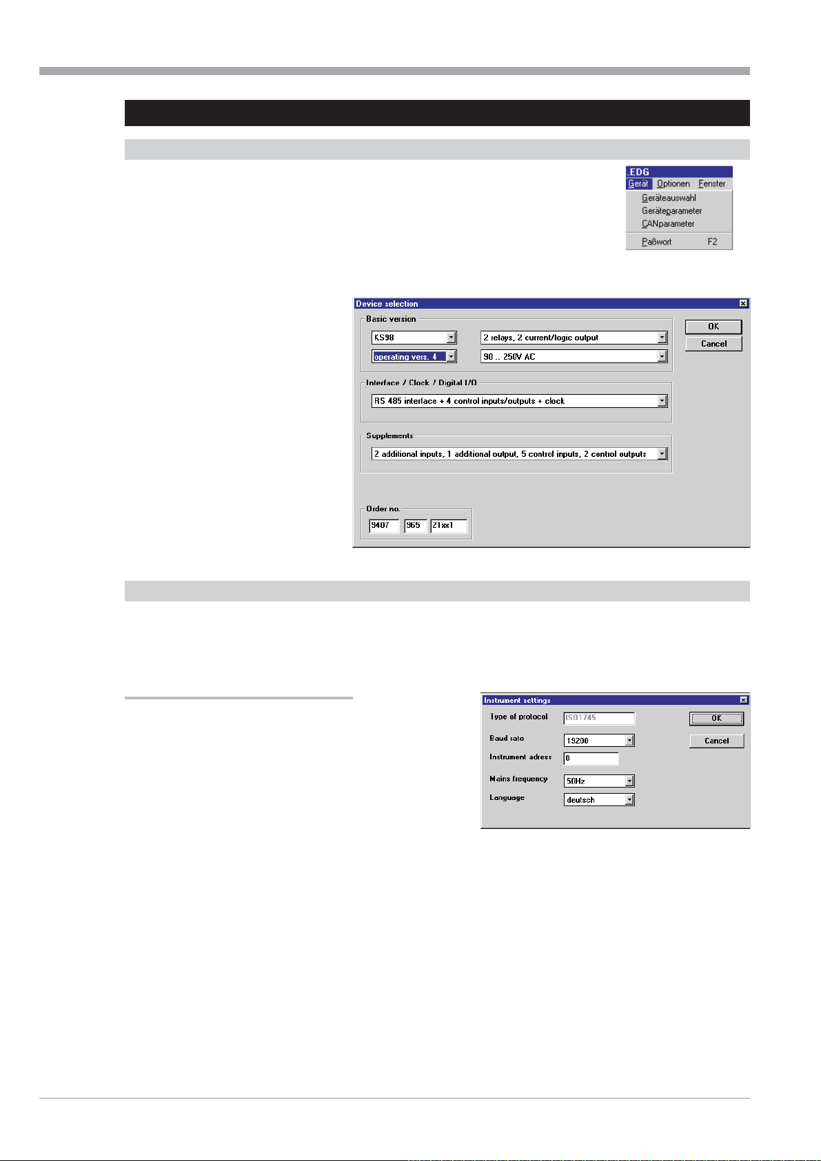
Menu reference to the engineering tool 9499-040-82711

II-3.5 Menu ‘Device’

Device selection

This command is used for selecting the KS 98-1 industrial controller version.

The mask displayed after execution of the command is displayed in Fig.:66.

Selection of the instrument version is possible via the drop-down items.

The order number resulting from the
version selection is displayed on the
bottom left. The inverse procedure

(entry of order number ? display of in
strument version) is also possible.

For storage of the selected setting, the
selection must be validated by clicking
on “OK”.

Clicking on button “Cancel” will cancel
the current selection.

Fig.: 66

-

Instrument parameters

In the input mask (r see Fig.: 67) the settings of KS 98-1 instrument data, address, Baudrate, mains frequency and
language are entered. These data are transmitted to KS 98-1, provided that the instrument version is correct.

Freezing the outputs for download

With this field enabled, the engineering is prepared in such a
way that during the next download to the multi-function unit,
the outputs are frozen in their present status. With the field dis
abled, the outputs are switched off during this time.

This means that the selected function only becomes

effective after the next download.

Fig.: 67

-

II-64 Menu ‘Device’

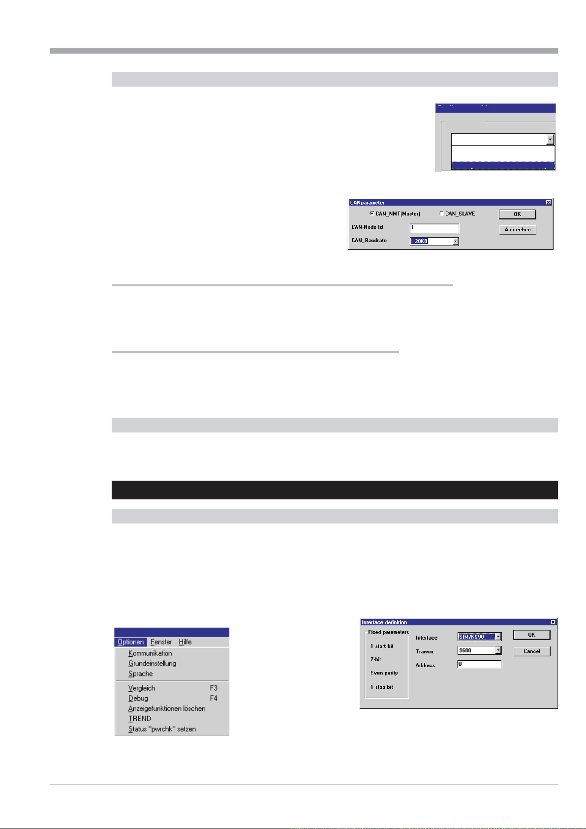
9499-040-82711 Menu reference to the engineering tool

CANparameter

The menu item “CANparameter” can only be selected, if “KS 98-1, CAN I/O ex

-

tension” has been enabled during device selection (see Fig.:68 ).

The window “CANparameter” (see Fig.:69 ) is used to define whether the device
is a CAN_NMT (Master) or a CAN_SLAVE. Make sure that the CAN_Baudrate
has been adjusted to the same transmission speed in the entire CAN network.

Various speeds between 10 kbytes and 1000 kbytes are selectable (default value
is 20 kbytes).

Fig.: 69

Fig.:68

Selecting device

Basic unit

KS 98-1, CAN I/O-Extension

KS 98-1
KS 98-1, with transm.

KS 98-1, CAN I/O-Extension

Communication between KS 98-1 and RM 200 modules, KS 800 or KS 816

KS 98-1 communicating with RM 200 modules, KS 800 or KS 816, must be defined as master. In this case, the CAN
node ID “1" is automatically assigned to the CAN_NMT (master).

Cross-communication with other KS 98-1 multifunction units

For the cross-communication between several KS 98-1, it is necessary to configure one KS 98-1 as the master, and the
other units as slaves. In this case, the CAN node ID “1" is automatically assigned to the CAN_NMT (master). The ad ­dresses 2...24 can then be assigned to the CAN_SLAVEs.

Password (F2)

The password can be adjusted and changed via this menu item. Password entry during transmission is possible addi ­tionally.

II-3.6 Menu ‘Options’

Communication

This menu item can be used for selecting the interface via which the interface cable is connected to the PC for commu
nication with Industrial Controller KS 98-1. Baud rate and device address are also adjustable. The other communication
parameters are fixed and displayed only for information (r see Fig.: 70). The function “Transmit address and bit rate”
refers to the communication parameters defined in the window “Device parameters” (see Fig.:66 ).

For storage of the selected setting, the selection must be acknowledged by clicking on “OK”. Clicking on button “Can
cel” will cancel the current selection.

Fig.:70

-

-

Fig.: 71

Menu ‘Options’ II-65

Menu reference to the engineering tool 9499-040-82711

Basic setting

Two display modes are possible. The hatched mode is recommended
for print-out on black-and-white printers or displays (e.g. laptop). In
all other cases, the colour setting should be used.

Fig.: 73

Language

The engineering tool language can be selected.

Fig.: 72

Comparison (F3)

Permits comparison of the active engineering with the contents of the connected KS 98-1 or of the simulation. The
operation is started immediately after clicking on this item. The comparison result is displayed in a message window.
Possible messages are shown in Fig.: 74 to Fig.: 76. (close window with key “x”).

Fig.: 74 Fig.: 75Fig.: 76

Debug (F4)

Activates cyclic display of signals in the additionally created monitor blocks
(see also chapter 3.5).

Deleting display functions

As display functions are not transmitted to KS 98-1, deleting all these functions at the end of the debug phase may
make sense.

Trend

See description of ‘Universal trend function’ (chapter 3.6 from page 72 )

Set status “pwrchk”

The STATUS function provides a digital output “pwrchk” (power fail check), which goes to “0" when the power returns
after a failure.

By means of the function “Set status pwrchk” this output can be reset to “1", thus enabling a functional test of the en
gineering to be triggered after a power failure.

II-66 Menu ‘Options’

-

9499-040-82711 Menu reference to the engineering tool

II-3.7 Menu ‘Window’

Error

The menu item “Error” enables an error message window to be displayed
or hidden, if errors occur during loading or when switching to another operating version.

Menu ‘Window’ permits selection of an error window, or returning to the background, if an error occurred during loa
ding or operating version switch-over.

Connecting diagram

-

Depending on the selected hardware version and the wired inputs/outputs, a connecting diagram is generated interac
tively, which also contains the assigned block names.

II-3.8 Menu ‘Help’

The engineering tool is delivered with an on-line help which is available
at any time. How to handle the Windows help system is described in detail in the documentation
of the Windows operating system.

Engineering INFO

After execution of this command, the following window with general
engineering information is displayed (r see Fig.:77).

-

Fig.: 77

Licence

Information on your entered licence number required with questions you may have is displayed in this information
window. A new licence number can be entered via button Change...

(r page 53 ).

Info

When selecting command Info in menu Help, an information window containing the version number and a gene
ral information on the engineering tool is displayed. You should
be able to specify this version number, whenever you should have any questions.

-

Menu ‘Window’ II-67

Engineering tool operation 9499-040-82711

II-4 Engineering tool operation

II-4.1 Fundamentals of the engineering tool operation

For operation of the engineering tool, basic knowledge of the Windows operating system is an advantage. Unless you
have this knowledge, please, make familiar with Windows first before executing the program for the first time. This is
possible using the Windows manual, the Windows on-line help and the Windows learning program.

For all questions in connection with the engineering tool, the KS 98-1 ONLINE HELP

q

(key F1) is available (r Menu Help).
Press the F1 key with the function marked or with the parameter dialogue opened to start

.

a

the on-line operating instructions (only possible with the Acrobat reader on the computer installed)

Before making changes to the engineering, the engineering must be stored, since changes cannot be can
celed automatically!

-

The two operating modes are distinguished by the mouse pointer display (hand symbol / arrow symbol). These two mo
des are described in the following sections. Switch-over is by double-click with the left mouse key or via ‘Menu’ r
‘Edit’ r ‘Positioning’/’Wiring’.

II-4.2 Function block placement

A function can be selected either via menu bar ‘Functions’ or ‘Fixed functions’, or by
entry of the function name in capital letters. With the engineering tool in the place­ment mode (mouse pointer is a hand symbol), the name of the instantaneously se­lected function is displayed in the bottommost status line.

By clicking with the right mouse key, the selected function is placed in the actual
mouse pointer position.

II-4.3 Function block shifting

After clicking with the mouse pointer on a function block, the mouse pointer is displayed inversely (r see Fig.:78) and
can now be shifted either by means of the cursor keys or using the mouse (keep left mouse key pressed). The linked
connection lines are dragged. Clicking with the right mouse key with inverse display of the function block opens the
parameter dialogue of this function (r see also page 61). Shifting several function blocks simultaneously is possible
only in the survey display (‘Edit’ r ‘Survey’ or by pressing key ‘a’).

Procedure:

Calling up the survey (key ‘a’).
Use the mouse pointer to draw a window
across the function blocks which are to
be shifted.
Use the cursor keys or left mouse key to
shift the selected area.
Only the function blocks which are fully
covered by the marking will be shifted.

-

Fig.: 78

Fig.: 79

II-68 Fundamentals of the engineering tool operation

9499-040-82711 Engineering tool operation

II-4.4 Creating connections

Connections can be created only between analog outputs and inputs or digital outputs and inputs. Connecting digital
outputs and analog inputs and vice versa is not possible!

Procedure:

Click on the end point of the output arrow with the left mouse key.
With the mouse key kept pressed, draw the connection to the arrow start of the required input.
Release the mouse key.

Fig.: 80 Fig.: 81

false correct

An output can be connected with several inputs. However, connecting an input with several outputs is not possible.
The connection is displaced according to a standard algorithm.

Connecting additional inputs

If a connection was selected, an additional input can be connected directly by clicking with the left mouse key with key
CTRL (Strg) pressed. Select a defined segment of a connection to determine at which segment the new connection is
made (see Fig: 82/ 86 and 87 /83 ).

Fig.: 82 Fig.: 83

Fig.: 86 Fig.: 87

Handling connections

For increasing the graphic display clarity, subsequent handling of the connection lines is possible. The left mouse key
can be used to select a line in the wiring mode (arrow symbol). The selected line is now displayed in a different colour
and thickness. If this line belongs to a network (an output is connected with several inputs), the relevant lines are dis
played in the colour of the selected line, but in normal thickness. Now, the individual segments of the selected line can
be shifted by positioning the mouse pointer on a segment and with the left mouse key kept pressed. The segments can
also be displaced using the cursor keys.

If further line segments are required, the last segment can be prolonged and displaced as a new segment ( r see Fig.:
85 and 84). In this way, max. seven variable segments can be created.

Function ‘Standard connection’ can be used for returning the selected line into its standard form (Function key F11).

-

Fig.: 84 Fig.: 85

Creating connections II-69

Engineering tool operation 9499-040-82711

Changing signal source connections

In order to prevent the necessity to delete all connections and to remake them manually to the new source when chan
ging the network wiring for another signal source, connecting a complete network to another source is possible. This is
done automatically by clicking on the signal source (output) and simply clicking on the new source with key Ctrl (Strg)
pressed. Thereby, all inputs are connected to the new source automatically.

Overlapping lines

Extensive engineerings frequently feature overlapping lines
which do not belong to a network.

Function key F5 can be pressed for searching the enginee

­ring for overlapping lines. The first line which is found will
be marked.

Pressing function key F6 will search in the engineering and
count how many overlappings are found. The line found last
will be marked.

To ensure the clarity of the engineering, these lines shall be
shifted apart, until line marking after pressing keys F5 or F6
stops.

With networks, concentration of lines running in parallel is
desirable. For this, seize a line at the segment which is pas­sed by all lines to be concentrated, and move the marked
segment across all network lines (r see Fig.:89 ) with the

Shift

key or the switch-over key pressed. Segment shifting
can be done also using the cursor keys. Concentration of the
segments belonging to a network is also caused by pressing
key F7. Note, however, that the catching area is limited
with this function!

Fig.: 88

Fig.: 89

-

Variable editor and virtual links

Via menu item ‘Fixed functions‘‘ET functions‘(r p. 63) data sources and destinations (analog and digital) can be se
lected and inserted into the engineering as special block (r Fig.: 90). These sources can be assigned to variable na
mes as with all other functions in the parameter dialogue. In the parameter dialogue of data destinations, the already
defined variables are displayed in a listbox from which the required variable can be selected and assigned. These
‘virtual’ links are interpreted as ‘full’ lines in KS 98-1. Thus e.g. auxiliary functions can be placed at the periphery of the
engineering without the need to draw confusing lines through the whole engineering, whereby clarity and readability
are improved considerably.
However, these special blocks and their variable names are not stored in KS 98-1 and cannot be reconstructed when
reading out directly from a KS 98-1. They are rather shown as full lines.

Fig.: 90

-

-

II-70 Creating connections

9499-040-82711 Engineering tool operation

II-4.5 Online operation

Display blocks (analog and digital)

In ‘Fixed functions‘ r ‘ET functions‘(r Fig.: 91) display blocks (X-Disp and d-Disp) can be selected and inserted into
the engineering as special block (r Fig.: 92).

Fig.: 91

Like all other functions, these blocks can be given names in the parameter dialogue. Via ‘Options‘ r ‘Delete display
functions‘, all display blocks can be deleted simultaneously e.g. after finishing the engineering test.

Fig.: 92

Debug

The debug mode can be enabled/disabled either via the menu item “Options r Debug” or directly with F4. Operating
data are then exchanged cyclically (approx. 0,5s) with the KS 98-1 or SIM/KS 98-1. The generated display blocks will
show the relevant values. Too many display blocks will extend the cycle time.

Parameters can be changed online using the parameter dialog. After confirmation with “OK”, they are transmitted to
the KS 98-1. The results are displayed immediately.

Parameter changes via the KS 98-1 front panel are not transmitted to the PC during the debug mode.

Online operation II-71

Engineering tool operation 9499-040-82711

II-4.6 Trend function

Survey of the characteristics

Apart from the trend function specially designed for “Controllers” (CONTR, CONTR+) of the simulation package SIM/KS
98-1, additional trend windows can be implemented. Each trend is able to display 7 analog values and 12 logic states
from the Engineering against a time axis. Several independent trend displays can be shown simultaneously.

As soon as the trend function(s) have been called (L1READ), and the Engineering has been transmitted to the KS 98-1
or SIM/KS 98-1, the trend dialog window is opened via the menu item <Options><TREND>.

Trend dialog window

w

This window is used to select the required trend function, its duration, and the time interval. Clicking the START
button initiates the trend recording function, and a display window is opened for the selected trend curve. In this
way, it is possible to open several display windows.

Display window
Two different scales can be assigned to any pair of measurement values, which simplifies interpretation of the trend
curves.
The length of the time axis is adjusted by means of “Sampling cycle time” and “Number of measurement values” (sam
ples) for each trend display. The time axis is either “absolute” with date and time (hh:mm:ss) or “relative” (changeable
during the recording).
The exact analog values are shown numerically at top left in the display window. If the cursor line is active, the analog
values can be read precisely at any point of time. Trend display can be stopped (frozen) and resumed; the measurement
continues in the background!
By holding down the left mouse key, the cursor can be used to mark an area for enlargement.
This zoom function is canceled via <View><Complete display>.

-

Fig.: 93 Trend display

II-72 Trend function

9499-040-82711 Engineering tool operation

Preparations in the ET/KS 98

The trend function is an application that runs independently of the Engineering Tool. The values to be displayed are re
ceived directly from the KS 98-1 or from the simulation software SIM/KS 98-1. Data trans-mission is executed via the
communication modules L1READ (blocks 1...20), which must first be configured. For each L1READ, 7 analog values and
12 logic statuses from the Engineering can be “connected”. Usually, a single L1READ is enough to display the charac
teristic values of an application in relation to each other. However, up to 20 display windows can be provided. Please
note that the com-munication load depends on the transmission cycle adjusted in each display window, and can cause
problems. Make sure that the following limits are not exceeded:

Übertragungszyklus Anzahl Trendfenster

1s ß 2
2s ß 4
4s ß 8
8s ß 16

Fig.: 94 Preparations in the KS 98-1 Engineering

-

-

Implementing the trend function

When the preparations in the Engineering have been completed, and
it has been transmitted to the KS 98-1 or SIM/KS 98-1, the trend di
alog box is opened directly from the Engineering Tool ET/KS 98 by
means of <Options><Trend>.

All the L1READ functions implemented in the Engineering, are dis
played in a list box with their assigned “names”, from where they
can be selected for display.

The lower part of the trend dialog box shows all the signals connected to the selected L1READ function, complete with
block number, block title, and connection description or variable name.

Trend function II-73

-

Fig.: 95 Implemented L1READ functions

-

Engineering tool operation 9499-040-82711

Fig.: 96 Trend dialog box (trend display not yet started)

Trend recording of the selected L1READ function can now be started directly with the “Start” button. The trend para

­meters can be changed previously by means of the “Change” button. The duration of the trend curve (visible time axis)
is determined by the product of “Sampling time x sampling steps”. Furthermore, you can define what happens after the
selected recording duration has expired: Either the recording is terminated (“Stop at end”) or continued (“Ring memo ­ry/moving”). With the second option, previous values are deleted!

Fig.: 97 Behaviour when recording time has expired

II-74 Trend function

9499-040-82711 Engineering tool operation

Displaying the trend curves

Clicking the “Start” button initiates the trend recording function and opens a display window. Values are displayed
from left to right. Via the buttons in the dialog box, the trend display can be stopped (STOP) or moved into the bac
kground (Invisible), whereby the display window is closed. The lower part of the dialog box now shows a numeric dis
play of the actual values of the connected variables.

Note:

1. When using the simulation software SIM/KS 98-1, the “Turbo” mode should always be switched off.

2. Before starting the universal trend, the controller trend of the SIM/KS 98-1 simulation should be terminated!

Fig.: 98 Trend-dialogwindow (trend running)

-

-

Fig.: 99 Graph window

Trend function II-75

Engineering tool operation 9499-040-82711

Buttons in the display window

Symbol Description Symbol Description

Open file Stop/continue trend recording

Save file Enable/disable cursor line

Transfer selected item to the clipboard memory Parameter dialog for trend adjustments

Print file Program information

Adapting the trend curves

The menu items <Extras><Options> in the
display window enable you to adapt the
trend curves (“Channel settings”). While
the trend recording is running, the “Chan
nel settings” window can also be opened
from the trend dialog box via <Op
tions><Dialog>. The “Channel settings”
are stored together with the Engineering in
the KS 98-1 or the SIM/KS 98-1. The follo­wing settings can be adapted:

Selection of the graphic curves (x)
Description (title)
Curve colour
Value ranges (min / max)
Assignment of the left / right scales to
variables
Time axis (absolute / relative)

-

Fig.: 100 Parameter adjustments of the trend curves

-

Calling the trend function without ET-KS 98

The settings in the trend dialog box are saved via the menu items <File><Save as ...> in the file name.dat. This enables
the trend dialog box to be opened by calling trend_di.exe, and the required trend recording to be started without the
Engineering Tool.

However, a KS 98-1 or the Simulation SIM/KS 98-1 with the corresponding Engineering must be connected.

It is also possible to open a display window directly by opening the corresponding file name.dat, if a link with
trend_di.exe is provided under Windows.

Subsequent trend analysis

The contents of a display window can also be saved as a name.trd file, that can be opened later for analysis and eva
luation. The cursor line, display options, and the zoom function are active.

II-76 Trend function

-

9499-040-82711 Building an engineering

II-5 Building an engineering

First steps with the KS98-1 engineering tool

In this chapter, we would like to help you getting started with a concise description:

1. Installing the required tool

2. Projecting/programming a small test project

3. Testing the required instrument behaviour in the simulation

4. Loading the project into KS 98-1

5. Testing the implemented functions

6. Hint to the function library and task-related structures

7. References to further detail information on tools and application

After automatic start via “Installation of PMA Tools”, you will find engineering tool KS 98-1-Tools ET/KS98, Sim98-1
and instrument simulation SIM/KS 98-1 on the PMA CD.

Follow the instructions for installation and enter your licence number after being requested to do so (separate numbers
for engineering tool and simulator). If you only want to test the KS 98-1 tools without obligation first, our personnel
will give you temporary licence numbers for the two tools. Without the licence numbers, you will be able to test the
two tools independently, however, without building up communication between instruments. In this case, transmission
of a test engineering to the instrument or to the simulation is not possible. For communication with the real instru ­ment, only

the engineering tool licence is required.

Ü

Start the engineering tool and select the required language (German/English/French) via menu Options .

*

Functions and fixed functions.

These menu items contain the function blocks for selection of

the relevant function descriptions in this manual.

Ö

As a simple beginner’s project, we want to build up a control
loop. For this, we need a process value input (analog input 1)
from the fixed functions and a positioning output for the con
troller correcting variable (analog output 1).

ä

We select the input block from the list by clicking with the left
mouse key.
Now, position the block on the left of the working surface by cli
cking with the right

mouse key.

Fig. 101

-

-

<<Klick

II-77

Building an engineering 9499-040-82711

For controlling, we also need a controller (in Functions - Controllers > CONTR).

This controller should be positioned behind the input.

#

The same we do with the OUT4 and place him below the controller.

<

In the next step, we have to soft-wire the function blocks, in order to provide a connection from the input via the con ­troller to the output.

For this purpose, we can select the wiring mode (via

>

menu Edit – Wiring or by a simple double-click). The
mouse pointer as an arrow is displayed.

We use it to draw a line from the tip of the AINP1
(red arrow right) output arrow to controller input ar­row X1 by (means of the left key).

y

Accordingly, we draw a connection from controller po
sitioning output Yout1 of the controller block to the
input arrow of output block OUT4.

All function blocks have still to be checked for correct parameter setting. AINP1 is set to 0-20mA as default, which is
OK to start with. OUT4 is relay to the first output. The controller default setting is “continuous control”, we set it to
2-point in the field "CFUNC".

Fig. 102

-

II-78

9499-040-82711 Building an engineering

For this purpose, we return to the

x

soft-wiring mode ( hand pointer ) and
click with the right

mouse key on the

Fig. 104

function block for which we are setting
the parameters. The individual parame

­ter dialogue of the selected function
block appears.

Now the parameter is selected with a

c

click into the text field. Its signification
is displayed in concise form in the bot

­tom field of the input mask.
When opening the input field by clicking
twice, a listbox for selection is offered.

When leaving the parameter dialogue

v

<<Klick

with OK, the block setting is completed.

The engineering for a simple control loop is also completed. Only the function test has still to be passed. For this, eit
her a KS 98-1 or the simulation are required.

The instrument settings are dependent on whether a simulator or a real instrument are used for testing:

Test with device

In the ETKS98 atr device-device selection the adjustment to the existing device is made.

Therefore the product-code-no. of the device (sideways on the typeplate) is written into the "order-number" field

With OK the adjustment is confirmed.

For communication with the device a serial connection

Fig. 103

(COMport from the PC) with the device via pc-adapter is
set up.

Check r Menu - Options - Communication in the
ETKS98, if the interface is set to Com 1.

Test with the Simulation

Start SIM-KS98-1. Select the version to be simulated
atr Menu -Settings-Device.

In the ETKS98 atr device-device selection fill in
the product-code-no of the simulation (written in the field
order-no of the simulation). Confirmed with OK.

For communication with the simulation, in the engineering-tool the interface is set to SIM/KS98-1 via the Menu Op
tions-Communication.

After all this preparations we can load our little test-project, via Menu File-Project->KS98-1-Engineering. All con
trol requests we confirm with OK.

-

-

-

II-79

Building an engineering 9499-040-82711

After Start-up, we see the adjacent controller page.

+

Now the setpoint is altered (See: page): Insert a setpoint and
confirm it. The controller will adapt the process value (simulated
by KS98-1 with its correcting variable reaction.

As a matter of fact, every controller must be matched to the pro
cess characteristics. This refers mainly to control parameters
Xp1, Tn and Tv.

For detailed information including the self-tuning function, plea
se, see section Controller CONTR, CONTR+ and PIDMA page: 223) in this manual.

Detailed information on this subject and on the self-tuning possibility is given in this manual and in section Controller
(CONTR, CONTR+ and PIDMA) of the operating instructions. The different KS 98-1 operating pages and the operating
principle of these pages are described in a separate document (operating manual) apart from the function-related ex
planations of this manual.

The actual internal values of the instrument/simulator can be observed in the engineering tool.

This is helpful mainly when locating engineering errors.

On menu item:

Fixed functions – ET Functions – X-Disp : Display of analog
value for debug mode , internal ET display items (analog/di-

gital) can be selected.

Fig. 105

Fig. 106

-

-

-

For these items, positioning and soft-wiring are done as for
function blocks.
F4 ( Options – Debug ) can be used to activate the value
display (see Fig.: Debug information).

.

Fig. 107: Debug Informationen

II-80

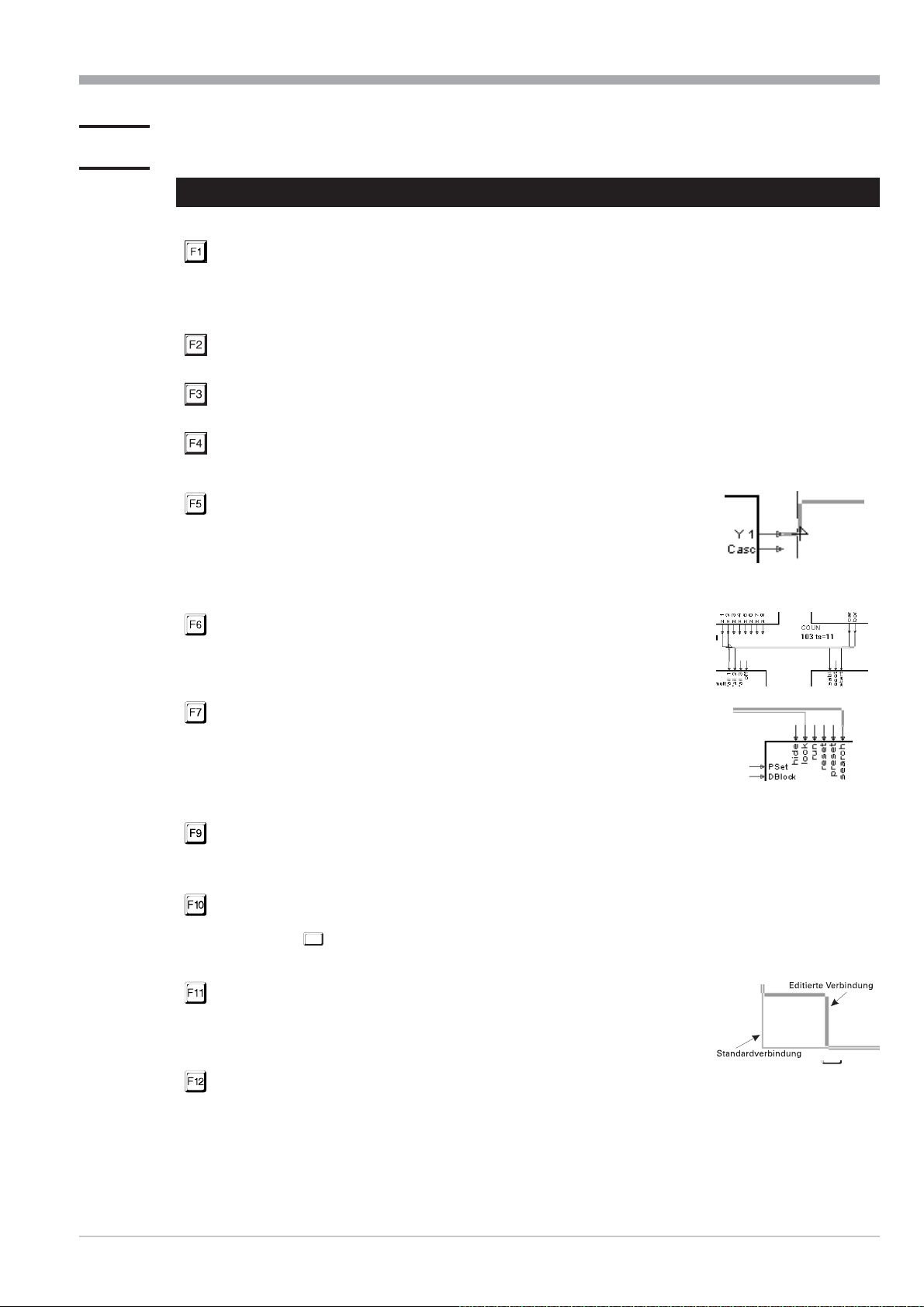
9499-040-82711 Tips and tricks

II-6 Tips and tricks

II-6.1 Function keys

Calling up the help ...

- General descriptions of the ET/KS 98 operating principle

- Survey and description of the library functions (with the function block selected or the
parameter dialog box opened). Prerequisite: The checkbox for help must have been clicked during installation.

Calling the password dialog

Comparison of the engineerings in KS 98-1 and ET is started.

Debug mode is activated

KS 98-1 or SIM/KS 98-1 must be connected!

Search line overlapping

During the wiring mode, line overlappings are searched. The first overlap
ping is displayed (shown marked). In the upper left
corner of the screen, either Acount=0" (result negative) or

Acount=1" is displayed.

-

Search all line overlappings

The overall engineering is searched for operlappings.
Overlappings found are displayed shortly on the screen, but only the last
overlapping found is displayed continuously.

Unify adjacent lines

Lines which belong to one connection, with only a few parallel
pixels, can be unified with F7. Thereby, a line segment must be selected.

(Shifting using the mouse may be not pixel-exact,
however, exact superposition is also possible by means of the
arrow keys.)

Line colour / -type of logic connections

On the screen, distinction of analog and logic connections is easier in colour. In a print-out (black and white), dis

tinction by a dashed line is better for clarity. Switch-over is always possible by pressing F9.

Cursor toggling between engineering i menu bar.

Menu operation with the arrow keys is now possible (if e.g. the mouse is not available). Function corresponds to

Alt

key .

Create standard connection

Connections of two dots are drawn automatically as short as possible at

right angles (standard connection) and can be edited manually. F11 trans

forms a selected edited connection into a standard connection.

-

Alt

-

Language selection

Language selection (German/English) for the engineering tool operator interface (menus, dialog boxes, etc.) is

possible during working in the main menu. However, the language of help texts for KS 98-1 functions can be se

lected only during installation!

-

Function keys II-81

Tips and tricks 9499-040-82711

Shift

+ click
(Wiring mode)

+ click

(Survey mode)

... Unify line segments

When shifting a line over other lines which belong to the same
signal source with the Shift key kept down, these lines are dragged and

superposed automatically after releasing the shifted line (start segments
cannot be shifted!). Closely adjacent lines are superposed automatically by
clicking on a connection with the shift key kept down.

Multiple connections

A signal source can be connected with several inputs by marking an already existing connection and clicking on

further inputs with the Strg key kept down. Thereby, the screen section can be shifted to the relevant position

using the scroll keys, if the input to be connected is out of the visible area.

A mouse click at any place on the screen with key ‘ pressed, will draw a grid that represents the print pages. In

the print-out, the pages are numbered linewisely from left to right and from top to bottom and can be printed out

with or without frame header.

Undo:

Cancels the last action..

Producing a black and white copy

The display window of the KS 98-1 is copied into the clipboard and can be

imported then to layout- or graphic-programs e.g. for documentation.

Alt

+Druck

copies the complete simulation into the clipboard (windows function)

II-6.2 Mouse key functions

Left mouse key Right mouse key

Edit mode

Wiring mode

Double-click on a free space:

r

Switches into the wiring mode

Click on a function block:

r

Selects (marks) the function block

Key held down:

r

Enables the function block to be moved.

Double-click on a free space:

r

Switches into the edit mode.

Click on a line:

r

Selects (marks) the line

Key held down:

Enables the line to be moved.

Click on a free space;

r

Inserts the previously selected function block.

Click on a function block:

r

Opens the parameter dialog of the block..

Click:

r

Switches into the survey display.

Survey

Click:

r

Switches into the wiring mode.

The position of the mouse pointer determines which
part of the engineering is placed in the center of the
wiring display.

II-82 Mouse key functions

9499-040-82711 Tips and tricks

II-6.3 Tips and tricks

Search

w

Entry of a block number (displayed in the upper left of the screen) and acknowledgement with Enter displaces the
screen and displays the searched function block with marking (functions also in the survey display).

Parameter setting

w

Double click in parameter input field selects the current value for entry. Triple click on P input field opens selecti
on dialog box (functions only once per parameter !) Setting cursor into value field with acknowledgement by pres
sing any key opens the selection dialog box (functions always !

Line segments

w

6 other line segments can be inserted into the last line segment (before the destination input), if the connection is
selected. For this purpose, seize the last line segment before the input and draw it into the required direction
using the mouse pointer in wiring mode.

Calculation sequence

w

The survey display can be used to show the calculation sequence.The sequence is indicated by consecutive mar
king of the function blocks.Start/stop of the marking procedure by means of the key “t”. While the procedure is
running, pressing key “r” stops the marking and moves back to the previous function block. Pressing key “v” mo
ves to the next function block.

-

-

-

-

w

Pixel-exact shifting of selected line (segments) and function blocks

COM test

w

Quick communication testing is possible by transmission of an "Empty" engineering to KS 98-1.
Testing the communication can also be done by calling up the password dialogue with without overwriting
the existing engineering. The password dialogue can be ended with ESC.

Copying parameters

w

If a function block is selected during the edit mode, its parameters can be stored in the clipboard by pressing

“C”. If another function block of the same type is then selected, the stored parameters can be copied into

the block by pressing “V”. This is a particularly useful feature for all blocks with many parameters (e.g.
CONTR; APROGD; ...). The function can also be used to transfer data into other engineerings, provided the same
operating version is involved.

Copying areas of the engineering

w

If an area has been selected in the survey display by means of the capture frame, its entire contents can be sto
red in the clipboard by pressing “C”. Pressing “V” copies the stored data into the engineering, where
it can be positioned with the mouse pointer. Parameters and internal connecting lines are maintained. External
connections are deleted.

Moving areas of the engineering

w

If an area has been selected in the survey display by means of the capture frame, its entire contents can be moved
with the mouse, if the key is held down. Parameters and internal connecting lines are redrawn automatically.

Shift

-

Abort

w

Time-consuming functions such as “Compare” (F3) can be aborted with the “x” key.

Block selection

w

Insiders enter the short-form name of the required function (e.g. ADSU) followed by acknowledgement to save the
detour via the menu bar. Click with the right mouse key to position the function thus selected directly (note up
per/lower case!). If the required function is quite close, selecting and de-selecting it is sufficient to produce the
same effect.

Tips and tricks II-83

-

Tips and tricks 9499-040-82711

Aligning blocks

w

Selected function blocks of the same type can be aligned in the "survey"
Key r up!
Key r left!

Searching for not connected "sinks"

w

Placed, but not defined signal sinks make an engineering more complex.

With the -key an internal list of all sinks not connected is set up.
With repeated pressing of or they can be found and either be
defined or deleted.

II-84 Tips and tricks

9499-040-82711 Tips and tricks

Tips and tricks II-85

Tips and tricks 9499-040-82711

II-86 Tips and tricks

9499-040-82711 Tips and tricks

Tips and tricks II-87

Tips and tricks 9499-040-82711

II-88 Tips and tricks

9499-040-82711

III Function blocks:

The KS98-1 function library contains all functions which are normally used for plant operation. These include:

Functions for calculation of mathematic formulas from simple addition to exponent function

w

Logic functions and functions for realization of control sequences

w

Numerous selection and storage functions are helpful for signal processing.

w

Alarm and limit value functions are indispensable for plant safety.

w

Interface functions facilitate communication with adjacent and supervisory systems.

w

Functions for implementation of complex and flexible control and program sequences as well as profile control

w

tasks meet the most exacting requirements.

The wiring principle of composed functions such as programmer, controller cascades and stepping control are explained in

the relevant basic function descriptions in this manual.

Examples for the basic engineering as mentioned in this manual, and further application examples for various require

ments are included on a CD as a collection of examples with detailed description, or available on request.

-

g

General KS 98-1 function block features

The features of multi-function unit KS 98-1 are determined by purposeful connection of standard function blocks with

adjustable parameters.

In the KS98-1 engineering, a function block represents a black box with analog inputs (from left), analog outputs (to

right), digital control inputs (from top) and control or status outputs (to bottom), as shown in the integrator diagram.

The following abbreviations are used for general inputs which mean process values and outputs which mean function

results:

analog inputs: X1, X2, ...

w

analog outputs: Y1, Y2, ...

w

digital inputs: d1, d2, …

w

digital outputs: z1, z2, ...

w

The abbreviations for inputs and outputs with special signification are

derived from their function.

III-89

9499-040-82711

Not all inputs and outputs of a function block need to be connected. The following rule is applicable: open inputs are
without effect. Examples: totalizer, multiplier, AND gate. In some cases, the connection of an input has an additional
effect, if e.g. priority handling is concerned (programmer control inputs).

Function blocks are numbered by the engineering tool in the order of occurrence from 100 to max. 450 as standard. Cal
culation of function blocks in the unit is dependent on this order. By changing the block number, the handling order is
adapted. Function blocks which can be used only once or with reference to the hardware (inputs/outputs) are always
within a numeric range of 0-100.

Function blocks are preset to a scanning rate (computing cycle) of 100 ms. The computing cycle can be increased to
800 in steps of 200, 400, whereby the processor load is reduced. Detailed information is given in the ET98 operating
manual.

The parameters of each function block are adjustable. Apart from an individual description for documentation purpo ­ses, the majority of blocks is provided with function-specific parameters. In addition to very special ones, some para ­meters are quite frequent. For these general values, the same identifiers are always used:

a, b, c, d factors without special signification
a0, b0, ... x0, y0 appended 0 as a symbol for an offset

x0 = offset of an input, y0 = offset of an output
T, Ti times in seconds (delays, pulse or pause duration)
Mode These parameters are used to select function parameter setting by means of the described parameter

or by means of an analog input (dynamic parameter setting).

Digital control inputs for binary selection (e.g. SELV1 for selection of 4 analog values) are normally numbered from left
to right d1, d2. Note that d2 is the less significant bit despite numbers running in opposed direction. In all cases where
the bit order also expresses an order of values, please, refer to the documentation of the special block in the following
chapters.

-

III-90

9499-040-82711 Scaling and calculating functions

III-1 Scaling and calculating functions

III-1.1 ABSV (absolute value (No. 01))

x1

a0a

yaxa

=×+

||

110

The absolute value of a number is it's number without polarity sign. This is the best solution for scaling a value that
can't become negative, in reference to calculating time. This function block should be used, when scaling must not use
a lot of calculating time.

Input variable x1is multiplied by factor a (parameter). Now, constant a0 is added. The absolute value of the resul
ting value is formed and output at y1.

Example:

y1= ABS(a w x1+ a0 ) a=5 x1=2 a0 = +5 results in y1=15
y1= ABS(a w x1+ a0 ) a=5 x1=2 a0 = -20 results in y1=10

Parameter Description Range Default

a
a0

Multiplication factor -29 999...999 999
Offset -29 999...999 999

III-1.2 ADSU ( addition/subtraction (No. 03))

A

y1

A

-

1
0

x1

a

x2

b

x3

c

x4

d

=× +× +× +× +

yaxbxcxdx y

112340

y0

y1

Input variables x1...x4 are multiplied by factors a...d. Constant y0 is added to the sum of evaluated inputs. Value
“0" is assigned automatically to unused inputs.

Parameter Description Range Default

a...d
y0

Multiplication factors -29 999...999 9990
Offset -29 999...999 999

1
0

ABSV (absolute value (No. 01)) III-91

Scaling and calculating functions 9499-040-82711

III-1.3 MUDI ( Multiplication / division (No. 05))

x1

a

x2

b

x3

c

ax a bx b

×+ ××+

AB

y

×

=

1

C

()()

=

10 20

Input variables x1...x3 are multiplied by factors a, b, c. The relevant constants a0, b0, c0 are added. The out
put variable corresponds to the product.

Value “1" is assigned automatically to unused inputs.
With divisions by “0" (C = c w x3 + c0 = 0) output y1 is set to 1.5 w 10

Parameter Description Range Default

a...c
a0...c0

Multiplication factors -29 999...999 999
Offset -29 999...999 999

III-1.4 SQRT ( square root function (No. 08))

A

a0

B

A*B

b0

c0

cx c

×+

C

C

30

y1

37

-

.

1
0

x1 y1

a

yaxa y

=×+ +

1100

a0

y0

Constant a0 is added to input variable x1 multiplied by a. The result is subjected to square root extraction.
Constant y0 is added to the result of square root extraction.

If the expression under the root is negative, the square root expression is set to 0. As a result: y1 =0.
If the input is not connected, this is interpreted as x1 =0.

Parameter Description Range Default

a
a0

Y0

Multiplication factors -29 999...999 999
Input offset -29 999...999 999
Output offset -29 999...999 999

1
0
0

III-92 MUDI ( Multiplication / division (No. 05))

9499-040-82711 Scaling and calculating functions

III-1.5 SCAL ( scaling (No. 09))

+

x1

a0a Exp

=×+()

yaxa

110

Input variable x1 is multiplied by factor a and added to constant a0.
The result (a w x1 + a0) is set to the power Exp.

If x1 is not used, this is interpreted as x1=0. With Exp = 0 SCAL outputs 1.

Parameter Description Range Default

a
a0
Exp

Example:

This function block should be used only, if the exponential function is needed. Factor a and the offset a0 are also avai ­lable with functions that need less calculating time (e.g. ADSU, MUDI, ABSV).

Multiplication factor -29 999...999 999
Offset -29 999...999 999
Exponent -7...7

2

11

11

2

3

yxxx

===

0,6

3

Exp

EXP

y1

1
0
1

III-1.6 10EXP (10s exponent (No. 10))

x1

Input value x1 is calculated according to formula
An unwired x1 is interpreted as x1 = 0 (in this case y1 is 1).

If the value at input x1 is higher than 36,7, an overflow may occur. In this case, output y1 is set to 1.5
than forming the power.

g

Note:
10EXP is the reversal function of function LG10.

x1

10

x11

10=

y

x11

and output at the y1 output.

10=

y

y1

1037rather

w

SCAL ( scaling (No. 09)) III-93

Scaling and calculating functions 9499-040-82711

III-1.7 EEXP (e-function (No. 11))

x1

The e-function is calculated.
If input signal x1 is higher than 85, there may be an overflow. In this case, y1 = 1,5
forming the power.

If x1 is not wired, this is interpreted as x1 = 0 and thus as y1 =1.

g

Note:
EEXP is the reversal function of function LN.

Examples:

With an input value of x1 = 5, output value y1 = 148,413159.
With an input value of x1 = 0,69314718, output value y1 =2.

III-1.8 LN (natural logarithm (No. 12))

x1

e

x11

=

ye

y1

1037is output rather than

w

g

x1

The natural logarithm of input variable x1 is formed.
The basis of natural logarithms is constant e (2,71828182845904).
If x1 is not wired, this is interpreted as x1 = 1. In this case y1 is 0.

With a negative input variable x1, y1 = -1,5

Note:
LN is the reversal function of function EEXP.

Examples:

The result of input value x1 = 63 is an output value of y1 = 4,143134726.
The result of input value x1 = 2,71828182845904 is an output value of y1 =1.

ln

yx

ln 1)= (

1

1037is set.

w

y1

III-94 EEXP (e-function (No. 11))

9499-040-82711 Scaling and calculating functions

III-1.9 LG10 (10s logarithm (No. 13))

g

x1

The common logarithm of input variable x1 is formed.

LG10 provided the logarithm of a number to base 10.
If x1 is not wired, this is interpreted as x1 = 1. In this case, y1 is 0.

With a negative input variable x1, y1 = -1,5

Note:
LG10 is the reversal function of function 10EXP.

Examples:

The result of input value x1 = 63 is an output value of y1 = 1,799340549.
The result of an input value x1 = 2,71828182845904 is an output value of y1 =1.

log

10

log 1)= (

yx

1

1037is set.

w

y1

LG10 (10s logarithm (No. 13)) III-95

Non-linear functions 9499-040-82711

III-2 Non-linear functions

III-2.1 LINEAR (linearization function (No. 07))

X1
Casc

LINEAR

Y1

100 ts=11

X1

Casc

y11

...

y2
y1

y

6

5

4

3

2

1

x1 x2 x11

...

10

9

8

7

Y1

x

Block LINEAR can be used for calculation ofy=f(x).

Max. 11 adjustable segment points for simulation or linearization of non-linear functions are available. Each segment
point comprises input x(1) and output y(1).

The segment points are connected automatically by straight lines. Each input value x1 has a defined output value y1.
With an input value x1 smaller than parameter x(1), the output value is equal to the y(1) value. If input value x1 ex ­ceeds the highest parameter x(n) value, the output value is equal to the relevant y(n) value.

The condition for input of configuration parameters is that values are input in ascendant order (x(1) < x(2) <...< x(11)).
The end of value pairs is marked by the “OFF” value in the next input value x(n+1).

This function block is cascadable. It has 2 inputs: The 1st input provides the variable which must be linearized. The
2nd input (case) is used to connect the previous linear block.

Inputs/outputs

Analog inputs

X

Casc

Input variable which must be linearized
Cascade input

Analog outputs

Y

Linearization result

Parameter

Parameter Description Range Default

x(1) ...
x(11)
y(1) ...
y(11)

Input value for segment point 1...11 -29999...999999, OFF

x(1)<x(2)<.....x(11)

Output value for segment point 1...11 -29999 ... 999 999

x(1) = 0, x(2) = 1, x(3) = 2, ...,

x(11) = 10

y(1) = 0, y(2) = 1, y(3) = 2, ...,

y(11) = 10

III-96 LINEAR (linearization function (No. 07))

9499-040-82711 Non-linear functions

Example: linear as a cascade

Fig. 108

II

X1

LINEAR

I

X

X1

Casc

LINEAR

Y1

Casc

Y1

Y

yI+yII

yI

LINEAR I

LINEAR I

(x11/y11)

x11

(x11/y11)

(x1/y1)

LINEAR II

x1

-

x

-

x

LINEAR (linearization function (No. 07)) III-97

Non-linear functions 9499-040-82711

III-2.2 GAP (dead band (No. 20))

y

x1

y=x-Low

y=x-High

x

y1

Low

=-

yx1Low

1

=

y0

1

=-

yx1High

1

High

bei x1 < Low
bei x1 = Low...High
bei x1 > High

The range of the dead band is adjusted with parameters Low (lower limit) and High (upper limit). If input value x1 is
within the dead band (Low ß x1 ß High), output value y1 =0.Ifx1 is not used, this is interpreted as x1=0.

Example:

In the following example, -10 for Low and 50 for High was used.

Fig. 109

y1

10

-20

-10

10

30

20

40

50

x1

Low= -10

-10

High= +50

Parameter Description Range Default

Low
High

Lower limit value -29 999...999 999
Upper limit value -29 999...999 999

0
0

III-98 GAP (dead band (No. 20))

9499-040-82711 Non-linear functions

III-2.3 CHAR (function generator (No. 21))

x1

y11

y2
y1

...

y

6

5

4

3

2

1

x1 x2 x11

7

...

8

Seg

10

9

y1

x

( 10)ß

With max. 11 adjustable value pairs, non-linear functions can be simulated or linearized. Each value pair comprises in
put x(1) and output y(1). The number of value pairs is determined using configuration parameter Seg (number of seg

-

ments +1 corresponds to the number of value pairs).
The value pairs are connected automatically with straight lines so that each input value x1 provides a defined output

value y1. If input value x1 is smaller than parameter x(1), the output value is equal to the value of y(1). If input
value x1 is higher than the highest parameter x(n) the output value is equal to the corresponding y(n) value.

During entry of the configuration parameters, the condition is that the assigned values stand in ascending order
(x(1) < x(2) <...< x(11)).

Configuration Description Range Default

Seg
x(1)...(11)

y(1)...(11)

Number of segments 1...10
Input value for curve point -29 999...999 999
Output value for curve point -29 999...999 999

2

0...10*

0...10*

* 0 for x(1) and y(1), 1 for x(2) and y(2) ... 10 for x(11) and y(11).

-

Unless

one CHAR is sufficient, the following tip might be helpful:

whereby x10 of CHARI=x1ofCHAR II and x11 of CHARI=x2ofCHAR II

Fig. 110

CHAR I

x10/Y10

x11/y11

I

CHAR

x2/y2

II

CHAR II

CHAR

x1/y1

CHAR I+II

ADSU

CHAR (function generator (No. 21)) III-99

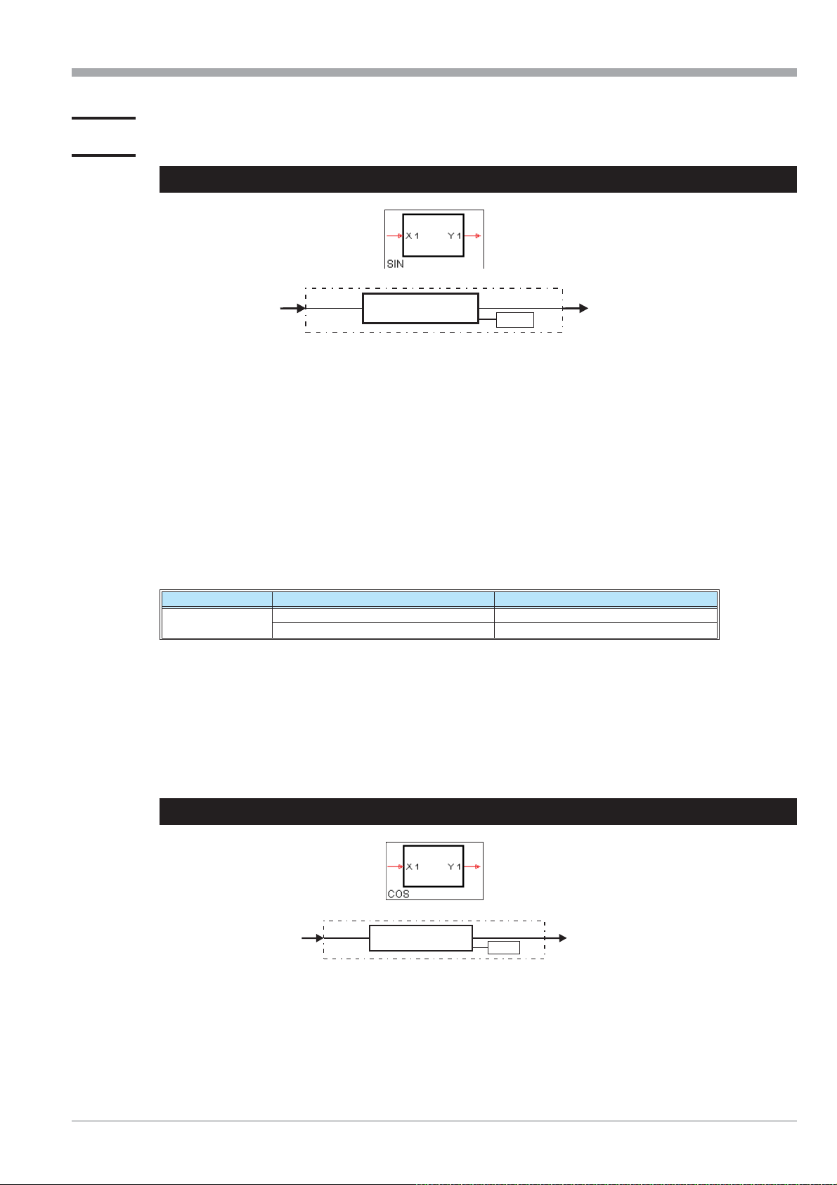
9499-040-82711 Trigonometric functions

III-3 Trigonometric functions

III-3.1 SIN (sinus function (No. 80))

x1

The function provides the sinus of the input value, i.e. x1 is the angle the sinus of which is calculated.
Parameter Select is used to adjust, if the angle is provided in degree of angle [°] or in radian.

The calculation clarity can be reached by limiting the input signal (e.g. to the 1st or 4th quadrant ( _90° / _
nal limiting is not provided. If input value x1 is out of the range in which the sinus function can still provide purpose
ful values, output y1 is set to 1,5 w 10

Example degree of angle:

y1= sin(x1) x1 = 30° = y1 = 0,5

Example radian:

y1= sin(x1) x1 = 90rad = y1 = 0,89399666

Parameter Description Controller display

Select

1 rad = 180°/ó = 57,296°
1°=ó/180° = 0,017453 rad

Unit: degree of angle (default) Ang. deg
Unit: radian Radian

(y1)=sin(x1)

yx

sin 1)= (

1

37

.

Select

y1

ó

/2)). Inter

-

-

Control with the pocket calculator:

The function for the calculation in "rad" with the pocket calculator is limited to e.g. ±8 ó.
r 90/ ó = 28,6479: sin ( 0,6479 wó) = 0,893996664

Also during input in "°" usually a limitation is effective in the pocket calculator (e.g. < 1440°)!

III-3.2 COS (cosinus function (No. 81))

x1

The function provides the cosinus of the input value, i.e. x1 is the angle the cosinus of which is calculated.
Parameter Select is used to adjust, if the angle is provided in degree of angle [°] or in radian.

(y1) =cos (x1)

yx

1

y1

Select

cos 1)= (

SIN (sinus function (No. 80)) III-100