West Control Solutions KS 45 User Manual

Download

PMA Prozeß- und Maschinen-Automation GmbH

Universal controller

KS 45

rail

line

Operating manual

9499-040-71811

KS 45

English

valid from: 06/2009

BlueControl

More efficiency in engineering, more overview in operating:

The projecting environment for the BluePort indicators and rail line - measuring converters / universal controllers

controllers,

ATTENTION!

Mini Version and Updates on

Explanation of symbols:

g a

© 2004 · PMA Prozeß- und Maschinen-Automation GmbH · Printed in Germany All rights reserved · No part of this document may be reproduced or published in any form or by any means without prior written permission from the copyright owner.

General information

General warning

Caution: ESD-sensitive components

Caution: Read the operating instructions

Read the operating instructions

Note

www.pma-online.de

or on PMA-CD

A publication of PMA Prozeß- und Maschinen Automation P.O.Box 310229 Germany

Content

1. General ............................................5

1.1 Application in thermal plants ..............................6

2. Safety hints ..........................................7

2.1 MAINTENANCE, REPAIR AND MODIFICATION ....................8

2.2 Cleaning .........................................8

2.3 Spare parts .......................................8

3. Mounting ...........................................9

3.1 Connectors .......................................10

4. Electrical connections ..................................11

4.1 Connecting diagram ..................................11

4.2 Terminal connections .................................11

4.3 Connecting diagram ..................................13

4.4 Connection examples .................................14

4.5 Hints for installation ..................................15

4.5.1 cULus approval .................................15

5. Operation ..........................................16

5.1 Front view .......................................16

5.2 Operating structure ..................................17

5.3 Behaviour after supply voltage switch-on.......................17

5.4 Displays in the operating level ............................18

5.4.1 Display line 1 ..................................18

5.4.2 Display line 2 ..................................18

5.4.3 Switch-over with the enter-key ........................18

5.5 Extended operating level ...............................19

5.6 Special change-over functions.............................20

5.6.1 Automatic / manual switch-over........................20

5.6.2 ProG - start programmer ............................20

5.6.3 Func - switching function ...........................20

5.7 Selecting the units ...................................21

6. Functions ..........................................22

6.1 Linearization ......................................22

6.2 Input scaling ......................................23

6.2.1 Input fail detection ...............................24

6.2.2 Two-wire measurement ............................24

6.3 Filter ..........................................25

6.4 Substitue value for inputs ...............................25

6.5 Input forcing ......................................25

6.6 O

2 measurement (optional) ..............................25

6.7 Limit value processing .................................27

6.7.1 Input value monitoring .............................27

6.7.2 Heating-current alarm .............................28

6.7.3 Loop-alarm ...................................29

6.7.4 Monitoring the number of operating hours and switching cycles ......29

6.8 Analog output (optional) ................................30

6.8.1 Analog output .................................30

6.8.2 Logic output ..................................31

6.8.3 Transmitter power supply ...........................31

6.8.4 Analog output forcing .............................31

6.9 Maintenance manager / error list ...........................32

6.9.1 Error list: ....................................32

6.9.2 Error status self-tuning.............................33

6.10 Resetting to factory setting ..............................34

7. Controlling .........................................35

7.1 Setpoint processing ..................................35

7.1.1 Setpoint gradient / ramp............................36

7.1.2 Setpoint limitation ...............................36

7.1.3 Second setpoint ................................36

7.2 Configuration examples ................................37

7.2.1 Signaller (inverse)/ On-Off controller .....................37

7.2.2 2-point controller (inverse) ...........................38

7.2.3 3-point controller (relay & relay) ........................39

7.2.4 3-point stepping controller (relay & relay)...................40

7.2.5 Continuous controller (inverse) ........................41

7.2.6 D - Y - Off controller / 2-point controller with pre-contact .........42

7.3 Self-tuning .......................................43

7.3.1 Preparation for self-tuning ...........................43

7.3.2 Self-tuning sequence .............................43

7.3.3 Self-tuning start ..............................44

7.3.4 Self-tuning cancellation ............................44

7.3.5 Acknowledgement procedures in case of unsuccessful self-tuning .....44

7.3.6 Examples for self-tuning attempts ......................45

7.4 Manual tuning .....................................46

8. Programmer .........................................47

9. Timer ...........................................49

9.1 Setting up the timer ..................................49

9.1.1 Operating modes ................................49

9.1.2 Tolerance band .................................50

9.1.3 Timer start ...................................50

9.1.4 Signal end ...................................50

9.2 Determining the timer run-time ............................50

9.3 Starting the timer ..................................51

9.4 End / cancelation of the timer .............................51

10.Configuration level.....................................53

10.1 Configuration survey ................................53

10.2 Configurations .....................................54

11.Parameter-level ......................................61

11.1 Parameter-survey ...................................61

11.2 Parameters .......................................62

12.Calibrating-level ......................................64

12.1 Offset-correction ....................................65

12.2 2-point-correction ...................................66

13.Engineering Tool BlueControl

.............................67

14.Versions ...........................................68

15.Technical data .......................................69

16.Index ...........................................74

1 General

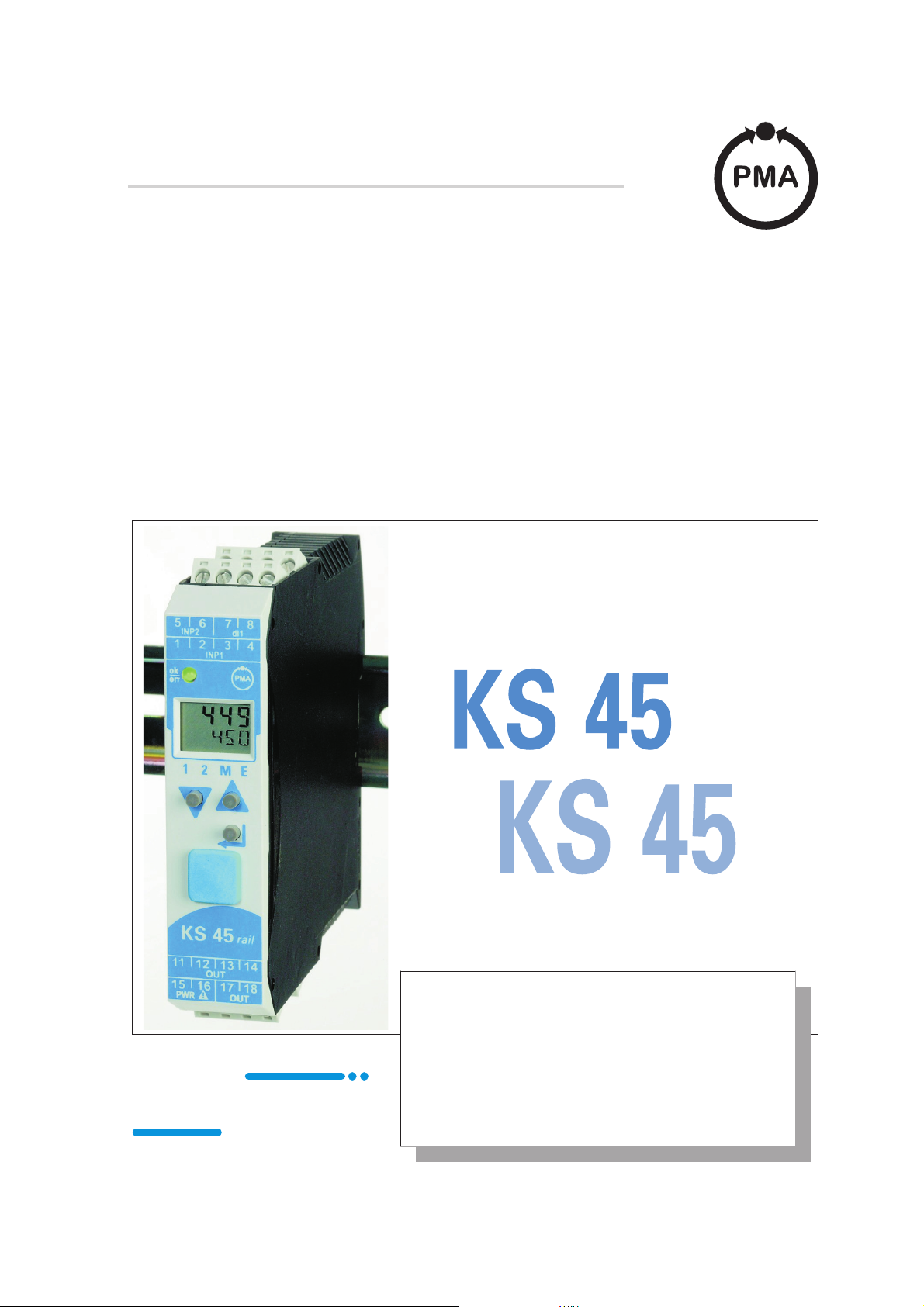
Thank you very much for buying an Universal Controller KS 45. The universal controllers KS 45 are suitable for precise, cost-efficient contol tasks in all industrial applications.

For that you can choose between simple on/off-, PID- or motorstepping control.

The process-value signal is connected via an universal input. A second analog input can be used for heating-current measurement or as external setpoint input. The KS 45 has at least one universal input and two switching outputs. Optionally the controller can be fitted with an universal output or with optocoupler outputs. The universal output can be configured as continuous output with current or voltage, for triggering solid state relays or for transmitter supply. Galvanic isolation is provided between inputs and outputs as well as from the supply voltage and the communication interfaces.

Applications

The KS 45 as universal controller can be utilized in many applications, e.g.:

...

Furnaces

Burners and boilers

Dryers

Climatic chambers

Heat treatment

Sterilizers

Oxygen-control

As a positioner

General

At-a-glance survey of advantages

Compact construction, only 22,5 mm wide

Clips onto top-hat DIN rail

Plug-in screw terminals or spring clamp connectors

Dual-line LC display with additional display elements

Process values always in view

Convenient 3-key operation

Direct communication between rail-mounted transmitters

Universal input with high signal resolution (>14 bits) reduces stock keeping

Universal output with high resolution (14 bits) as combined current / voltage output

Quick response, only 100 ms cycle time, i.e. also suitable for fast signals

2-Pt.-, 3-pt.-, motorstepping-, continuous controlling

Customer-specific linearization

Measurement value correction (offset or 2-point)

Self-optimization

Logical linking of digital outputs, e.g. for common alarms

Second analog input for ext. setpoint, heating current or as universal input

Further documentation for universal controller KS 45:

–

Data sheet KS 45 9498 737 48513

–

Operating note KS 45 9499 040 71541

–

Interface description 9499 040 72011

KS 45 5

General

1.1 Application in thermal plants

In many thermal plants, only the use of approved control instruments is permissible. There is a KS 45 version (KS45-1xx-xxxxx-Dxx) which meets the requirements as an electronic temperature controller (TR, type 2.B) according to DIN 3440 and EN 14597. This version is suitable for use in heat generating plants, e.g. in

building heating systems acc. to DIN EN 12828 (formerly DIN 4751)

•

large water boilers acc. to DIN EN 12953-6 (formerly DIN 4752)

•

heat conducting plants with organic heat transfer media acc. to DIN 4754

•

oil-fired plants to DIN 4755

•

…

Temperature monitoring in water, oil and air is possible by means of suitable approved probes.

Application in thermal plants 6KS45

2 Safety hints

This unit was built and tested in compliance with VDE 0411-1 / EN 61010-1 and was delivered in safe condition. The unit complies with European guideline 89/336/EWG (EMC) and is provided with CE marking. The unit was tested before delivery and has passed the tests required by the test schedule. To maintain this condition and to ensure safe operation, the user must follow the hints and warnings given in this operating manual.

Safety hints

The unit is intended exclusively for use as a measurement and control instrument in technical installations.

Warning

If the unit is damaged to an extent that safe operation seems impossible, the unit must not be taken into operation.

ELECTRICAL CONNECTIONS

The electrical wiring must conform to local standards (e.g. VDE 0100). The input measurement and control leads must be kept separate from signal and power supply leads. In the installation of the controller a switch or a circuit-breaker must be used and signified. The switch or cir cuit-breaker must be installed near by the controller and the user must have easy access to the controller.

COMMISSIONING

Before instrument switch-on, check that the following information is taken into account:

Ensure that the supply voltage corresponds to the specifications on the type label.

•

All covers required for contact protection must be fitted.

•

If the controller is connected with other units in the same signal loop, check that the equipment in

•

the output circuit is not affected before switch-on. If necessary, suitable protective measures must be taken.

The unit may be operated only in installed condition.

•

Before and during operation, the temperature restrictions specified for controller operation must

•

be met.

a a

Warning The ventilation slots must not be covered during operation.

The measurement inputs are designed for measurement of circuits which are not connected directly with the mains supply (CAT I). The measurement inputs are designed for transient voltage peaks up to 800V against PE.

SHUT-DOWN

For taking the unit out of operation, disconnect it from all voltage sources and protect it against accidental operation. If the controller is connected with other equipment in the same signal loop, check that other equipment in the output circuit is not affected before switch-off. If necessary, suitable protective measures must be taken.

KS 45 7

Safety hints

2.1 MAINTENANCE, REPAIR AND MODIFICATION

The units do not need particular maintenance. There are no operable elements inside the device, so the user must not open the unit

Modification, maintenance and repair work may be done only by trained and authorized personnel. For this purpose, the PMA service should be contacted.

Warning

When opening the units, or when removing covers or components, live parts and terminals may be exposed. Connecting points can also carry voltage.

Caution

When opening the units, components which are sensitive to electrostatic discharge (ESD) can be exposed. The following work may be done only at workstations with suitable ESD protection. Modification, maintenance and repair work may be done only by trained and authorized personnel. For this purpose, the PMA service should be contacted.

You can contact the PMA-Service under:

PMA Prozeß- und Maschinen-Automation GmbH Miramstraße 87 D-34123 Kassel

Tel. +49 (0)561 / 505-1257 Fax +49 (0)561 / 505-1357 e-mail: mailbox@pma-online.de

2.2 Cleaning

The cleaning of the front of the controller should be done with a dry or a wetted (spirit, water) handkerchief.

2.3 Spare parts

As spare parts für the devices the following accessory parts are allowed:

Description Order-No.

Connector set with screw terminals 9407-998-07101 Connector set with spring-clamp terminals 9407-998-07111 Bus connector for fitting in top-hat rail 9407-998-07121

MAINTENANCE, REPAIR AND MODIFICATION 8KS45

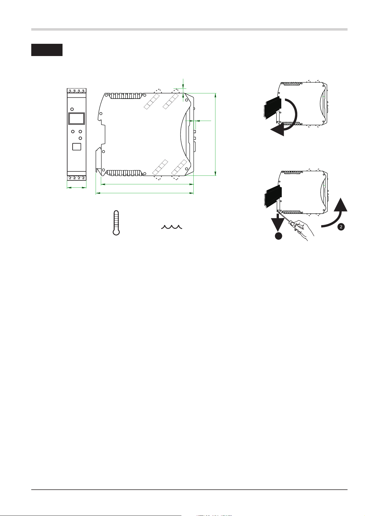
3 Mounting

Mounting

bmessungen / dimensions

22.5

(0,87”)

max.

117.5 (4,63”)

55°C

-10°Cmin.

111 (4, 37 ”)

max. 95% rel.

Klemme /

1516

terminal

Klemme /

terminal

Montage / mounting

5.5 (0,20”)

2.3

(0,08”)

click

99 (3,90”)

Demontage / dismantling

11 1 2

a a a

l a

The unit is provided for vertical mounting on 35 mm top-hat rails to EN 50022. If possible, the place of installation should be exempt of vibration, aggressive media (e.g. acid, lye), liquid, dust or

aerosol. The instruments of the rail line series can be mounted directly side by side. For mounting and dismounting, min. 8 cm

free space above and below the units should be provided. For mounting, simply clip the unit onto the top-hat rail from top and click it in position.

To dismount the unit, pull the bottom catch down using a screwdriver and remove the unit upwards.

Universal Controller KS 45 does not contain any maintenance parts, i.e. the unit need not be opened by the customer.

The unit may be operated only in environments for which it is suitable due to its protection type.

The housing ventilation slots must not be covered.

In plants where transient voltage peaks are susceptible to occur, the instruments must be equipped with additional protective filters or voltage limiters!

Caution! The instrument contains electrostatically sensitive components .

Please, follow the instructions given in the safety hints.

To maintain contamination degree 2 acc. to EN 61010-1, the instrument must not be installed below contactors or similar units from which conducting dust or particles might trickle down.

KS 45 9

Mounting

3.1 Connectors

The four instrument connectors are of the plug-in type. They plug into the housing from top or bottom and click in posi tion (audible latching). Releasing the connectors should be done by means of a screwdriver. Two connector types are available:

Screw terminals for max. 2,5 mm2conductors

•

Spring-clamp terminals for max. 2,5 mm2conductors

•

Before handling the connectors, the unit must be disconnected from the supply voltage.

Tighten the screw terminals with a torque of 0,5 - 0,6 Nm. With spring-clamp terminals, stiff and flexible wires with end crimp can be

introduced into the clamping hole directly. For releasing, actuate the (or ange) opening lever.

Contact protection: Terminal blocks which are not connected should remain in the socket.

Connectors 10 KS 45

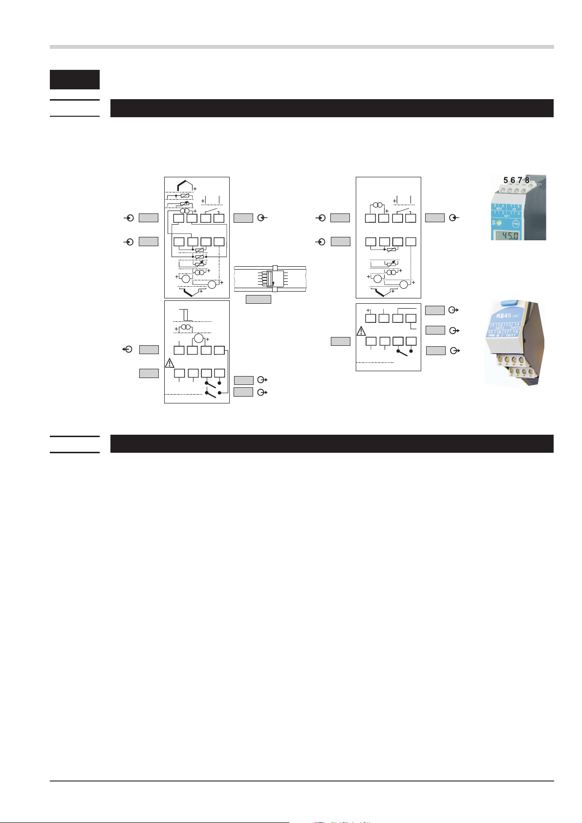
4 Electrical connections

4.1 Connecting diagram

Electrical connections

KS45-1xY-xxxxx-xxx

=0,1,2,3

(mV)

b c

INP2

INP1

OUT3

PWR

a b c d

90...260V AC 24V AC/DC

Logic

b a

di1

OUT1

OUT2

RGND

Data A Data B

RS 485

KS45-1xY-xxxxx-xxx

=4,5

1234

11 12 13 14

15 16 17 18

AC / DC

INP2

INP1

top

RGND

Data A Data B

PWR

24VDC

90...260V AC 24V AC/DC

b a

di1

OUT1

OUT2

OUT3

4.2

Terminal connections

Faulty connection might cause destruction of the instrument !

1 Connecting the supply voltage

Dependent on order

90 … 260 V AC terminals: 15,16

•

24 V AC / DC terminals: 15,16

•

For further information, see section "Technical data"

Instruments with optional system interface: Energization is via the bus connector of field bus coupler or power supply module. Terminals 15, 16 must not be used.

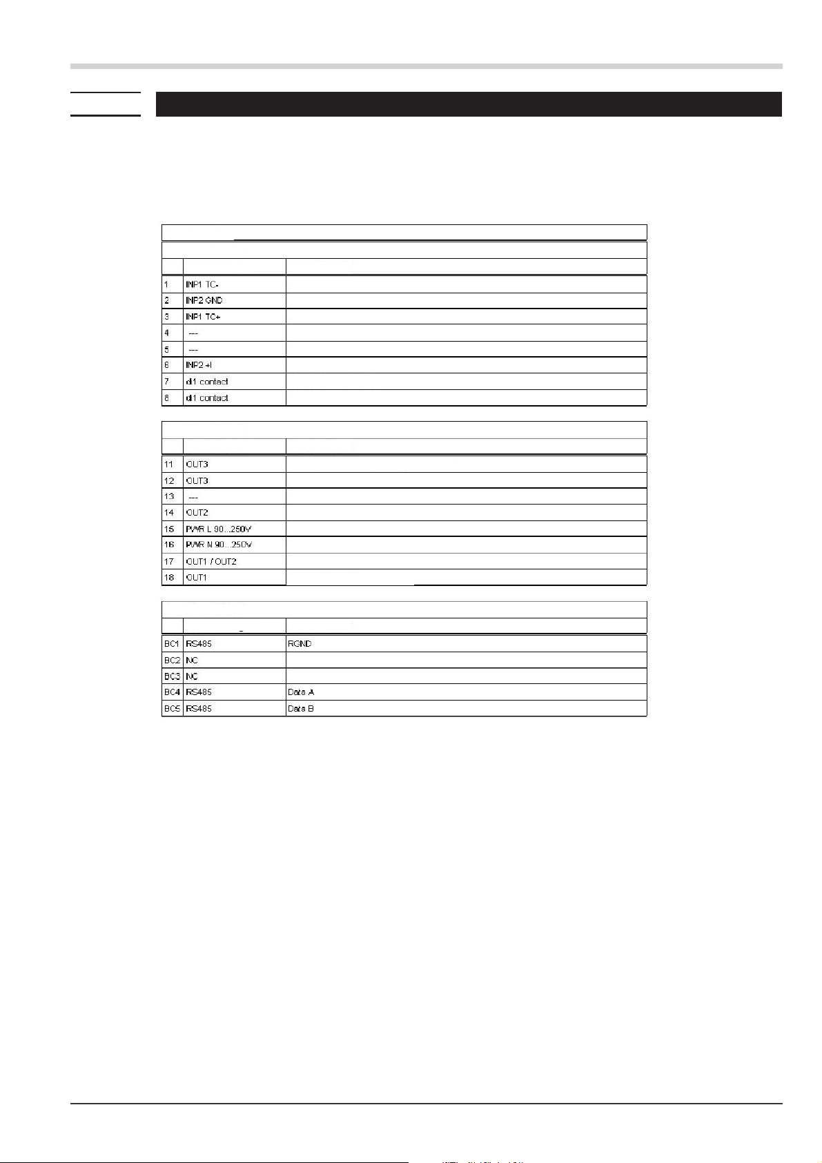
2 Connecting input INP1

Input for the measurement value

a resistance thermometer (Pt100/ Pt1000/ KTY/ ...), 3-wire connection terminals: 1, 2, 3 b resistance thermometer (Pt100/ Pt1000/ KTY/ ...), 4-wire connection terminals: 2, 3, 5, 6 c potentiometer terminals: 1, 2, 3 d current (0/4...20mA) terminals: 2, 3 e voltage (-2,5...115/-25...1150/-25...90/ -500...500mV) terminals: 1, 2 f voltage (0/2...10V/-10...10V/ -5...5V) terminals: 2, 4 g thermocouple terminals: 1, 3

KS 45 11 Connecting diagram

Electrical connections

3 Connecting input di1

Digital input, configurable as a switch or a push-button.

a contact input terminals: 7,8 b optocoupler input (optional) terminals: 7,8

4 Connecting outputs OUT1 / OUT2 (optional)

Relay outputs max. 250V/2A NO contacts with a common terminal.

•

5 Connecting output OUT3

Universal output

h logic (0..20mA / 0..10V) terminals: 11,12 i current (0...20mA) terminals: 11,12 j voltage (0...10V) terminals: 12,13 k transmitter power supply terminals: 11,12

6 Connecting the bus interface (optional exept d)

RS 485 interface with MODBUS RTU protocol

* see interface description MODBUS RTU: (9499-040-72011)

OUT1 terminals: 17, 18 OUT2 terminals: 17, 14

7 Connecting input INP2 (optional exept d)

Input for the second variable INP2.

a thermocouple terminals: 5,6 b resistance thermometer (Pt100/ Pt1000/ KTY/ ...), 3-wire connection terminals: 2,5,6 c potentiometer terminals: 2,5,6 d current (0/4...20mA) terminals: 2,6 e voltage (-2,5...115/-25...1150/-25...90/ -500...500mV) terminals; 5,6

8 Connection of input INP1 for the version with optional opto-coupler outputs

Input for the measured variable (measurement value).

a resistance thermometer (Pt100/ Pt1000/ KTY/ ...), 3-wire connection terminals: 1, 2, 3 c potentiometer terminals: 1, 2, 3 d current (0/4...20mA) terminals: 2, 3 e voltage (-2,5...115/-25...1150/-25...90/ -500...500mV) terminals: 1, 2 f voltage (0/2...10V / -10...10V / -5...5V) terminals: 2, 4 g thermocouple terminals: 1, 3

9 Connecting INP2 -HC (optional)

Input for heating current

Current 0/4...20mA DC and0…50mAAC terminals: 5,6

•

0 Connecting opto-coupler outputs OUT1 / OUT2 (optional)

Opto-coupler outputs with shared positive control voltage.

OUT1 terminals: (11), 12, 13

•

OUT2 terminals: (11), 12, 14

•

! Connecting relay output OUT3 (optional)

Relay output max. 250V/2A as nomally open contact.

OUT3 terminals: 17, 18

•

Terminal connections 12 KS 45

4.3 Connecting diagram

The instrument terminals used for the engineering can be displayed and printed out via BlueControlÒ( menu File \ Print preview - Connection diagram).

Example:

Connecting diagram

Connector 1

Name

Connector 2

Name

Description

Process value x1

Description

Signal limit 1, signal INP1 fail

Electrical connections

Heating current input

Switch-over to SP2

Connector 3

Name

Controller output Y2

Controller output Y1

Description

KS 45 13 Connecting diagram

Electrical connections

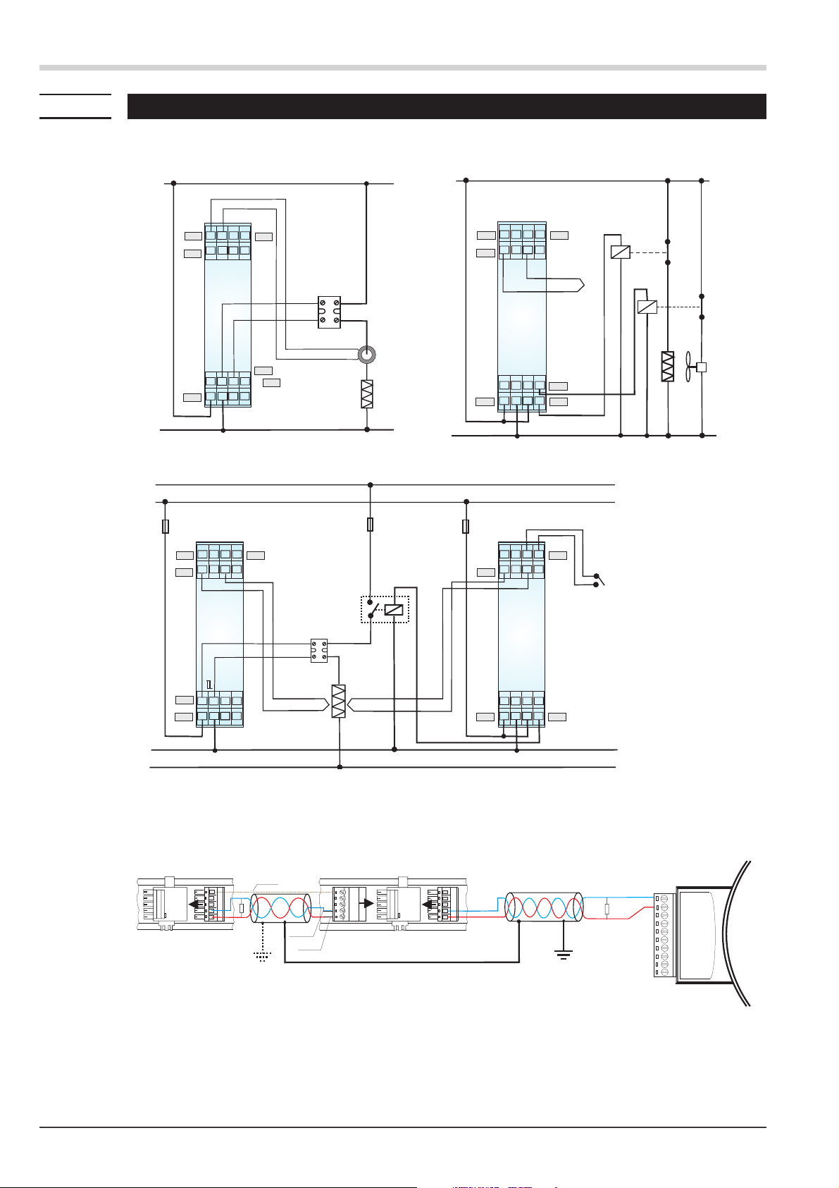
4.4 Connection examples

Example: INP2 with current trans- former and SSR via opto-coupler

INP2

INP1

PWR

di1

SSR

OUT1

OUT2

Connection example: KS 45 and TB 45

Fuse

INP2

INP1

KS 45

di1

Fuse

contactor

Example: heating / cooling OUT 1 /OUT2

TB 45

di1

OUT2

OUT1

di1

Resetbutton

Fuse

INP2

INP1

PWR

temperature limiter

INP1

heating

SSR

OUT3

PWR

Logic

PWR

Example: RS 485 interface with RS 485-RS 232 converter See documentation 9499-040-72011

Master z.B. / e.g.

Converter RS 232-RS 485

RGND

LT 1

Data A

Data B

Data A

Data B

(ADAM-4520-D)

LT 1

DATA+ 1

DATA-

TX+ TXRX+

RX-

(R)+Vs (B)GND 10

(RS-485)

(RS-422)

Connection examples 14 KS 45

4.5 Hints for installation

Measurement and data lines should be kept separate from control and power supply cables.

Sensor measuring cables should be twisted and screened, with the screening connected to

earth. External contactors, relays, motors, etc. must be fitted with RC snubber circuits to manufacturer

specifications. The unit must not be installed near strong electric and magnetic fields.

The temperature resistance of connecting cables should be selected in accordance with the

local conditions.

Electrical connections

a a

4.5.1 cULus approval

The unit is not suitable for installation in explosion-hazarded areas.

Faulty connection can lead to the destruction of the instrument.

Please, follow the instructions given in the safety hints.

For compliance with cULus regulations, the following points must be taken into account:

Use only copper (Cu) wires for 60 / 75 °C ambient temperature.

The connecting terminals are designed for 0,5 – 2,5 mm2Cu conductors.

The screw terminals must be tightened using a torque of 0,5 – 0,6 Nm.

The instrument must be used exclusively for indoor applications.

For max. ambient temperature: see technical data.

Maximum operating voltage: see technical data.

KS 45 15 Hints for installation

Operation

5 Operation

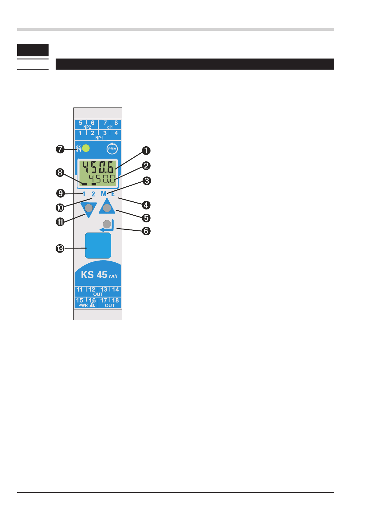
5.1 Front view

1 Line 1: process value display 2 Display 2: setpoint /output value/ unit-display / extended

operating level / errolist / values from Conf- and PArA-level special functions as A-M, Func, run, AdA

3 operating mode “manual” 4 Error list (2 x ô ), e.g.

· Fbf. x sensor fault INP. X

· sht. x short circuit INP. X

· Pol. x wrong polarity INP. X

· Lim. x limit value alarm

· ...

5 Increment key 6 Enter key to select extended operating level or error list 7 Status indicator LEDs

· green: limit value 1 OK

· green blinking:no data exchange with bus coupler

(only on instruments with optional system interface)

· red: limit value 1 active

· red blinking: instrument fault, configuration mistake

8 Display elements, active as bars 9 Status of switching output OUT1 active 0 Status of switching output OUT2 active ! Decrement key

§ PC connection for the BlueControl

engineering tool

Front view 16 KS 45

In the first LCD-display line the measured value is shown. The second LCD-line normally shows the setpoint. When changing over to the parameter setting, configuration or calibration level and at the extended operating level, the parameter name and value are displayed alternately.

§ : To facilitate withdrawal of the PC connector from the instrument, please, press the cable left.

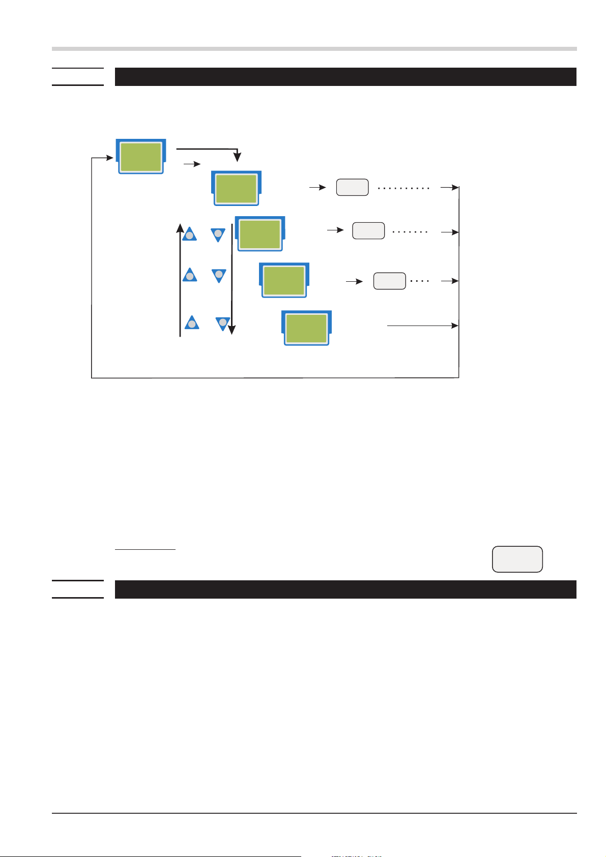
5.2 Operating structure

The instrument operation is divided into four levels:

Operation

450.3

450.0

äüüü

The access to the parameter, configuration and calibrating level can be disabled using the following two methods:

Level disabling by adjustment in the engineering tool (IPar, ICnf, ICal). Display of disabled levels is suppressed.

450.3

PARA äüüü

450.3

CONF äüüü

450.3

CAL äüüü

450.3

END äüüü

PASS

Operating level

Parameter level

Configuration level

Calibrating level

The access to a level can be disabled by entry of a pass number (0 … 9999). After entry of the

adjusted pass number, all values of the level are available. With faulty input, the unit returns to the operating level. Adjusting the pass number is done via BlueControl

Individual parameters which must be accessible without pass number, or from a disabled parameter level, must be copied into the extended operating level.

Factory-setting:

all levels are accessible without restrictions, pass number PASS = OFF

5.3 Behaviour after supply voltage switch-on

After switching on the supply voltage, the instrument starts with the operating level. The operating status is as before power-off.

If the device was in manual mode, when switching off the power-supply, it also starts up in manual mode with output value Y2.

PASS

KS 45 17 Operating structure

Operation

5.4 Displays in the operating level

5.4.1 Display line 1

The displayed value, also named process value, is shown in the first display line. This value is used as controlled value (variable). It results from the configuration C.tYP. (also see chp./page 7-22.)

5.4.2 Display line 2

The value to be displayed continuously in the second LCD line can be selected from different values via the

BlueControl

Normally the internal setpoint SP is set.

engineering tool.

450.3

450.0

äüüü

By deleting the individual settings for display 2, it is resetted to setpoint display. Reset to display of the engineering unit is possible by deleting the entry for line 2.

With faulty input values, signals dependent on the inputs (e.g. Inp1, Inp2, display value, Out3) also indicate FAIL.

5.4.3 Switch-over with the enter-key

By using the enter-key, different values can be called in display 2. Every time you press the enter key, the display jumps to the next feature as shown below.

450.3

mAn

ä äüü

1 Default settings as setpoint 2 Display of operating mode

automatic/manual

Displaying the defined display 2 value (via BlueControlÒ). Standard setting is the internal setpoint

Displaying the output value, e.g. Y57

Calling up the error list, if messages are supplied. If there is more than one message with every push of the enter key the next message is displayed.

Calling up the extended operating level, if messages are supplied. If there is more than one message with every push of the enter key the next message is displayed.

Returning to the original displayed value. If for 30 s no key is pushed, the display automatically returns to the origin.

450.3

450.0

äüüü

450.3

Y57

ä üüü

450.3

FbF.1 ä üüü

450.3

L.1 ä üüü

450.3

450.0

äüüü

Displays in the operating level 18 KS 45

5.5 Extended operating level

The operation of important or frequently used parameters and signals can be allocated to the extended operating level.

This facilitates the access, e.g. travelling through long menu trees is omitted, or only selected values are operable, the other data of the parameter level are e.g. disabled.

Display of the max. 8 available values of the extended operating level is in the second LCD line.

The content of the extended operating level is determined by means of the BlueControl select entry "Operation level" in the "Mode" selection menu. Further information is given in the on-line help of the engi neering tool.

450.3

äüüü

ûC

engineering tool. For this,

Press key ô to display the first value of the extended operating level (after display of error list, if necessary).

The selected parameters can be changed by pressing keys Ì and È .

Operation

450.3

H.I äüüü

ô press to display the next parameter

450.3

500.0

äüüü

450.3

L.I äüüü

ô return to normal display after the last parameter

450.3

100.0

äüüü

Unless a key is pressed within a defined time (timeout = 30 s), the operating level is displayed again.

Extended operating level 19 KS 45

Operation

5.6 Special change-over functions

In order to operate switch-over or -on functions needed more often via front, there are special functions available.

A-M

•

Switch-over automatic / manual-operation

ProG

•

starting / stopping the programmer

Func

•

Selection of different switching signals

Via the engineering tool BlueControl function can be adjusted in the operating mode (sig nals/logic). It can be assigned permanently to display 2 or the extended operating level.

5.6.1 Automatic / manual switch-over

the desired

Between automatic and manual operation can be switched with the A-M function via front.

5.6.2 ProG - start programmer

For A-M function handling, the switch-over source must be set to “Interface only” (Conf / LoGI / mAn = 0).

Manual operation ist selected via the È - key. The display element M is activated.

If adjustment of the output value is allowed (Conf / Cntr / mAn = 1), the output value is displayed, otherwise display element (M) blinks.

The Ì - key switches to automatic operation. The function can be taken into the extended operating level, or perma nent in display 2.

If the programmer function is activated, (Conf / Cntr / SP.Fn = 1/9), with this function the programmer can be started (run) or stopped (OFF) via front. With the È - key the programm is started and stopped with the Ì - key.

After the end of a programm the stop function (OFF) must be selected before the programm can be started again.

450.3

Auto

äüüü

450.3

mAn

дьдьь

5.6.3 Func - switching function

The switching function Func takes the tasks of a function key. One or more signals switching at the same time, can be selected via configuration (Conf / LOGI/x=5)ausgewählt werden.

The switching function is set to on (= 1) via the È - key and to OFF (= 0) via Ì - key.

Example: The setpoint range adjustable by the user is limited from 20 to 100. Nevertheless it shall be possible to switch off the controller via front. This can be done by assigning Conf / LOGI / C.oFF= 5 and taking the Func - value into the extended operating level.

Special change-over functions 20 KS 45

Function Func is not suitable for timer activation.

5.7 Selecting the units

The unit to be displayed is determined via configuration D.Unt. With selection “1 = temperature unit” , the displayed unit is determined by configuration Unit with the relevant

conversions for Fahrenheit and Kelvin. By selecting D.Unt = 22, display of any max. 5-digit unit or text can be determined.

Operation

4.5

kWh

1 Unit (example): kilowatt hour 2 Text (example): TAG no.

äüüü

450.3

TI451 äüüü

For permanent display the value signals/other/D.Unt must be set in the mode "operating level" via the engineering

tool.

Selecting the units 21 KS 45

Functions

6 Functions

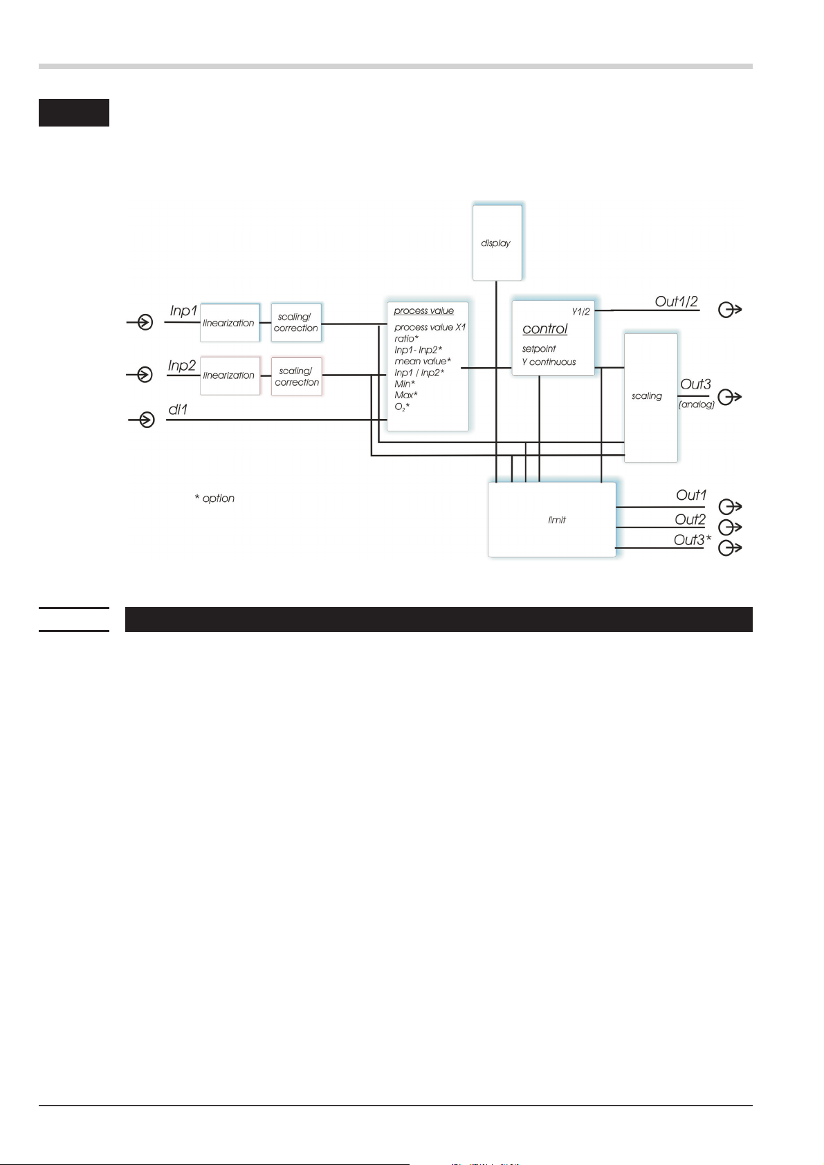
The signal data flow of transmitter KS 45 is shown in the following diagram:

6.1 Linearization

The input values of input INP1 or INP2 can be linearized via a table.

By means of tables, e.g. special linearizations for thermocouples or other non-linear input signals, e.g. a container filling curve, are possible.

Table “ Lin” is always used with sensor type S.TYP= 18: "Special thermocouple" in INP1 or INP2, or if linearization S.Lin = 1: “Special linearization” are adjusted.

w w

Non-linear signals can be linearized using up to 16 segment points. Each segment point comprises an input ( In.1 … In.16) and an output (Ou.1 … Ou.16). These segment points are interconnected automatically by straight lines. The straight line between the first two segment points is extended downwards and the straight line between the two highest segment points is extended upwards, i.e. a defined output value for each input value is provided.

With an In.x value switched to OFF, all further segments are switched off.

Required: Condition for the input values is an ascending order.

In.1 < In.2 < ...< In.16.

For linearization of special thermocouples, the ambient temperature range should be defined exactly, becauseit is used to derive the internal temperature compensation.

The input signals must be specified in mV, V, mA, % or Ohm dependent on input type. For special thermocouples (S.tYP = 18), specify the input values in mV, and the output values in

the temperature unit adjusted in U.LinT . For special resistance thermometer (KTY 11-6) (S.tYP = 23), specify the input values in Ohm, and

the output values in the temperature unit adjusted in U.LinT.

See also page 60.

Linearization 22 KS 45

Ou.16

. . . . . .

Ou.1

1In

Functions

The same linearization table is used for input 1 and input 2.

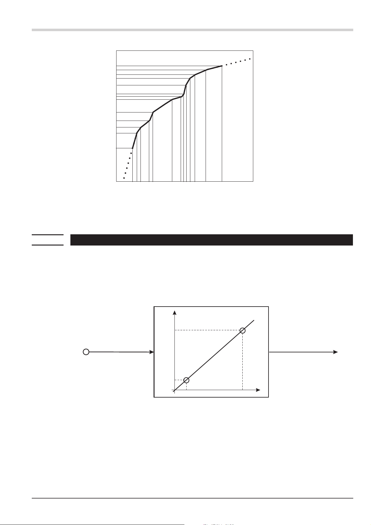
6.2 Input scaling

Scaling of input values is possible. After any linearization, measurement value correction is according to the offset or two-point method.

When using current or voltage signals as input variables for InP.x, the input and display values should be scaled at the parameter level. Specification of the input value of the lower and upper scaling point is in units of the relevant physical quantity.

Example for mA/V

mA / V

phys.

quantity

OuH.x

OuL.x

InL.x

InH.x

phys. quantity

mA/V

KS 45 23 Input scaling

Parameters InL, OuL, InH and OuH are visible only with ConF / InP / Corr = 3 selected.

Parameters InL and InH determine the input range.

Example with mA: InL= 4 and InH = 20 means that measuring from 4 to 20 mA is required (life zero setting).

- preliminary - Functions

For using the pre-defined scaling with thermocouples and resistance thermometers (Pt100), the settings for InL and OuL as well as for InH and OuH must correspond with each other.

For resetting the input scaling, the settings for InL and OuL as well as InH and OuH must correspond.

6.2.1 Input fail detection

For life zero detection of connected input signals, variable adjustment of the response value for FAIL detection is pos sible according to formula:

Fail response value £ In.L - 0,125 * (In.H - In.L)

Example 1: In.L = 4 mA, In.H =20mA

Fail response value £ 2mA

Example 2: In.L =2V,In.H =6V

Fail response value £ 1,5 V

6.2.2 Two-wire measurement

Normally, resistance and resistance thermometer measurement is in three-wire connection, whereby the resistance of all leads is equal. Measurement in four-wire connection is also possible for input I. With this method, the lead resistance is determined by means of reference measurement. With two-wire measurement, the lead resistance is included directly as a falsification in the measurement result. However, determination of the lead resistances by means of is possible.

Besides the connection of the both leads of the RTD / R sensor the 3rd connector has to be short-circuited.

Procedure with Pt100, Pt1000

Connect a Pt100 simulator or a resistance decade instead of the sensor at the test point so that the lead resistance is included and calibrate the values by means of 2-point correction.

By means of measurement value correction the resulting temperature value will be corrected, but not the resistance input value. In this case the linearization error can increase.

Procedure with resistance measurement

Measure the lead resistance with an ohmmeter and subtract it from the measured value via the scaling.

INP2

INP1

KS 45 24 Input scaling

6.3 Filter

Input values can be smoothened with an 1st order mathematical filter. Time constant is adjustable.

6.4 Substitue value for inputs

If a substitute value for an input is activated, this value is used for further calculation with a sensor fault, independent of the selected input function. The selected controller output reaction on sensor fault, configuration FAIL, is omitted.

With factory setting, the substitute value is switched off.

Functions

Before activation of a substitute value In.F, the effect on the control loop must be considered.

6.5 Input forcing

Setting f.AIx = 1 (only via BlueControl®) can be used for configuring the input for value entry via the interface (=forc ing).

Please, check the effect on the control loop in case of failure of input value / communication and exceeded measuring range.

6.6 O2 measurement (optional)

This function is available only on instrument versions with INP2 . Lambda probes (l probes) are used as input signals. The electromotive force (in volt) delivered by lambda probes is de-

pendent on the instantaneous oxygen content and on the temperature. Therefore, the device can only display accurate measurement results, if the probe temperature is known.

The instrument calculates the oxygen content according the Nernst formula.

Distinction of heated and non-heated lambda probes is made. Signals from both types can be handled by the device.

Heated lambda probes

Heated l probes are fitted with a controlled heating, which ensures a continuous temperature. This temperature must be specified in parameter Probe temperature in transmitter CI 45. Parameters ® Functions ® Pro be temperature tEmP ® ...°C (/°F/K - dependent on configuration)

Non-heated lambda probes

When the probe is always operated at a fixed, known temperature, the procedure is as with a heated probe. A non-heated l probe is used, if the temperature is not constant. In this case, the temperature in addition to the probe mV value must be measured. For this purpose, any temperature measurement with analog input INP2 can be used. During function selection, input INP2 must be set for measurement (CONF/InP.2/I.Fnc=1).

Configuration: O

-measurement must be adjusted in function 1 :

Func r Fnc.1 7

Connection

Connect the input for the lambda probe to INP1 . Use terminals I and 2. If necessary, temperature measurement is connected to INP2.

Input 1 is used to adjust one of the high-impedance voltage inputs as sensor type:

Filter 25 KS 45

O2-measurement with constant probe temperature (heated probe)

O2-measurement with probe temperature measurement

(non-heated probe)

Functions

41 special ( -2,5...115 mV) 42 special ( -25...1150 mV)

Inp.1r S.tYP

These high-impedance inputs are without break monitoring. If necessary, input signal monitoring is possible via the limit values.

Further recommendations for adjustment:

43 special ( -25...90 mV) 44 special ( -500...500 mV) 47 special ( -200...200 mV)

Input 1 must be operated without linearization:

Inp.1r S.Lin 0 no linearization

With O2 measurement, specification if parameters related to the measured value should be output in ppm or % is required. This is done centrally during configuration.

othrr O2 0 Unit: ppm

1 Unit: %

Whether the temperature of the non-heated l probe is entered in °C, °F or K can be selected during configuration.

othrr Unit 1°C

2°F 3K

Displays

With configuration for O2 measurement (see above), the oxygen content is displayed as process value with the selected unit (see above) on line 1. Max. 4 characters can be displayed.

With display range overflow, “EEEE” is displayed . Example: the ppm range is selected, but the value is a % value. When exceeding the display span start, 0 is displayed.

20.95

üû/o

O2 measurement (optional) 26 KS 45

Tip: the unit can be displayed on line 2.

6.7 Limit value processing

Max. three limit values can be configured for the outputs. Generally, each one of outputs Out.1... Out.3 can be used for limit value or alarm signalling.

Several signals allocated to an output are linked by a logic OR function.

6.7.1 Input value monitoring

Functions

The signal to be monitored can be selected separately for each alarm in the configuration. The following signals are available:

Process value (display value)

•

Control deviation (process value - setpoint)

•

Control deviation with suppression at start up or setpoint modification

•

Measurement value INP1

•

Measurement value INP2 (option)

•

setpoint

•

Output value

•

* After switch-on or setpoint change, the alarm output is suppressed, until the process value is within the limits for the first time. If a time limit (Src.x = 2) was configured, the alarm is activated after elapse of time 10 x ti1 (paramter ti1 = integral time). ti1 switched off (ti1 = OFF) is considered as ¥ , i.e. the alarm activation is omitted until the process value is within the limits once.

Each of the 3 limit values Lim.1 … Lim.3 has 2 trigger points H.x (Max) and L.x (Min), which can be switched off individually (parameter = “OFF”). The hysteresis HYS.x of each limit value is adjustable.

Input value monitoring is as shown below:

operating principle with absolute alarm

L.1 = OFF

operating principle with relative alarm

L.1 = OFF

Display range

Limit value 1

Outputs

Display range

Limit value 1 Outputs

-1999

H.1

HYS.1

L.1

LED rot / red

H.1

H.1 = OFF

L.1

HYS.1

LED rot / red

9999

-1999

LED

H.1

H.1 = OFF

L.1

HYS.1

9999

HYS.1

LED

9999

Limit value processing 27 KS 45

Functions

Display range

Limit value 1

-1999

H.1

L.1

Outputs

LED

rot / red

Normally open: ( ConF / Out.x/O.Act = 0 ) (as shown in the example) Normally closed: ( ConF / Out.x/O.Act = 1 ) (inverted output relay action)

6.7.2 Heating-current alarm

For the measured heating current; different alarms can be activated.

Overlaod heating current: Heating current is larger than limit value HC.A.

•

Interrupt heating current: Heating current is smaller than limit value HC.A.

•

For both, short-circuit alarm is integrated.

•

Short circuit monitoring

Current flow in the heating circuit although the controller output is switched off is considered as a short circuit e.g. in the solid-state relay and error message SSr (as an alarm in the error list, if configured) is output.

L.1

HYS.1 HYS.1

H.1

9999

LED

rot / red

-1999

LED

HYS.1

L.1

H.1

HYS.1

9999

LED

If the heating current is not measured as an AC current input S.tYP = “31 current 0...50mA AC”, the filter time constant must be t.Fx = 0, to prevent generation of an SSR alarm due to the filter effect.

With heating current measurement via INP1, note additionally that the cycle time of connected actuators should be > 10 s due to internal hardware filters.

With SSR short circuit alarm output, the output will be within the limits again only after alarm acknowledgement.

Heating current overload

If the current flow in the heating current circuit is higher than the adjusted heating current limit value ( HC.A), error message HC.A (as an alarm in the error list, if configured) is output.

Heating current interruption

If the current flow in the heating current circuit is lower than the adjusted heating current limit value ( HC.A), error message HC.A (as an alarm in the error list, if configured) is output.

With heating current alarm output, the output is within the limits again immediately, when the heating current returns within the limits.

Limit value processing 28 KS 45

6.7.3 Loop-alarm

An alarm can be activated, monitoring the control-loop for break. A break of the heating current loop is recognized, when at output of correcting variable Y=100% and elapsed sequence time 2 x ti1 (reset time), no appropriate reaction of the process value results.

Loop alarm can not be used with motor-stepping- or proportional-controller and signaller.

During self-tuning, loop monitoring is omitted.

6.7.4 Monitoring the number of operating hours and switching cycles

Operating hours

The number of operating hours can be monitored. When reaching or exceeding the adjusted value, signal InF.1 is acti vated (in the error list and via an output, if configured).

Functions

The monitoring timer starts when setting limit value C.Std. Reset of signal InF.1 in the error list will start a new moni toring timer. Monitoring can be stopped by switching off limit value C.Std.

Adjusting the limit value for operating hours C.Std can be done only via BlueControl®.

The current counter state can be displayed in the BlueControl

The number of operating hours is saved once per hour. Intermediate values are lost when switching off.

Number of switching cycles

The output number of switching cycles can be monitored. When reaching or exceeding the adjusted limit value, signal InF.2 is activated (in the error list and via an output, if configured).

The monitoring timer starts when setting limit value C.Sch. Reset of signal InF.2 in the error list will start a new moni toring timer. Monitoring can be stopped by switching off limit value C.Sch.

A switching cycle counter is allocated to each output. Limit value C.Sch acts on all switching cycle counters.

Adjusting the limit value for the number of switching cycles C.Sch can be done only via BlueControl®.

The current counter state can be displayed in the BlueControl

The number of switching cycles is saved once per hour. When switching off, intermediate values are lost.

expert version.

KS 45 29 Limit value processing

Functions

6.8 Analog output (optional)

6.8.1 Analog output

The two output signals (current and voltage) are available simultaneously. Adjust ConF / Out.3 / O.tYP to se lect the output type which should be calibrated.

ConF / Out.3: O.tYP = 1 Out.3 0...20mA continuous

= 2 Out.3 4...20mA continuous = 3 Out.3 0...10V continuous = 4 Out.3 2...10V continuous

phys.

size

Out.1

phys. size

Out.0

0/4mA

0/2V

Parameter O.Src defines the signal source of the output value. Example:

O.Src = 3 signal source for Out.3 is

Scaling of the output range is done via parameters Out.0 and Out.1. The values are specified in units of the physical quantity.

Out.0 = -1999...9999 scaling Out.3

Out.1 = -1999...9999 scaling Out.3

Example: output of the full input range of thermocouple type J (-100 … 1200 °C)

Out.0 = -100 Out.1 = 1200

Example: output of a limited input range, e.g. 60.5 … 63.7 °C)

Out.0 = 60.5 Out.1 = 63.7

20mA

10V

the process value

for 0/4mA or 0/2V

for 20mA or 10V

mA / V

g g

Analog output (optional) 30 KS 45

Please, note: the smaller the span, the higher the effect of input variations and resolution.

Using current and voltage output in parallel is possible only in galvanically isolated circuits.

Configuration O.tYP = 2 (4 … 20mA) or 4 (2...10V) means only allocation of the reference value (4 mA or 2V) for scaling of output configuration Out.0. Therefore, output of smaller values is also possible rather than output limiting by reference value 4mA / 2V.

Configuration O.tYP = 0/1 (0/4...20mA) or 2/3 (0/2...10V) determines, which output should be used as a calibrated reference output.

6.8.2 Logic output

The analog output can also be used as a logic output (O.typ = 0). In this case, e.g. alarms or limit values can be output or the output can be used as controller output.

6.8.3 Transmitter power supply

Two-wire transmitter power supply can be selected by adjusting O.typ =5. In this case, the analog output of the device is no longer available.

Connecting example:

Functions

INP2

INP1

OUT3

PWR

6.8.4 Analog output forcing

By adjusting f.Out = 1 (only via BlueControlÒ), the output can be configured for value input via interface, or by means of an input value at extended operating level (=Forcing).

di1

?13V 22mA

OUT1

OUT2

g g

KS 45 31 Analog output (optional)

This setting can be used also for e.g. testing the cables and units connected in the output circuit.

This function can also realize a setpoint potentiometer.

Functions

6.9 Maintenance manager / error list

In case of one or several errors, the error list is always displayed at the beginning of the extended operating level .

A current input in the error list (alarm or error) is always indicated by display of

letter E .

For display of the error list, press key ô once.

E- display element

blinks

off no error, all alarm entrys deleted

6.9.1 Error list:

Name

E.1

E.2

E.3

E.4

FbF.1

Sht.1

POL.1 FbF.2

Sht.2

POL.2

HCA

SSr

LooP

450.3

äüüä

Description Possible remedial action

Alarm due to existing error

Error removed, Alarm not acknowledged

Description Cause Possible remedial action

Internal error, cannot be corrected

Internal error, resettable

Configuration error, resettable

Hardware error Code number and hardware not

INP1 sensor break Defective sensor

INP1 short circuit Defective sensor

INP1 polarity error Wiring error Change INP1 polarity INP2 sensor break Defective sensor

INP2 short circuit Defective sensor

INP2 polarity error Wiring error Change INP2 polarity Heating current

alarm (HCA)

Heating current short circuit (SSR)

Control loop alarm (LOOP)

- Determine the error type in the error list via the error number

- remove error

- acknowledge alarm in the error list by pressing the È -orthe Ì -key

- the alarm entry is deleted by doing so

E.g. defective EEPROM Contact PMA service

Return device to manufacturer

E.g. EMC trouble Keep measuring and supply cables separate. Pro-

tect contactors by means of RC snubber circuits

Missing or faulty configuration Check interdependencies for configurations and

parameters Contact PMA service

identical

Wiring error

wiring error

Wiring error

Heating current circuit interrup ted, I< HC.A or I> HC.A (de pendent of configuration)

Heater band defective Current flow in heating circuit at

controller off SSR defective , bonded Input signal defective or not

connected correctly Output not connected correctly

Replace electronics/options card Replace INP1 sensor

Check INP1 connection Replace INP1 sensor

Check INP1 connection

Replace INP2 sensor Check INP2 connection

Check heating current circuit

If necessary, replace heater band

Check heating current circuit If necessary, replace solid-state relay

Check heating or cooling circuit Check sensor and replace it, if necessary

Check controller and switching device

ûC

Maintenance manager / error list 32 KS 45

Functions

Name

AdA.H

AdA.C

Lim.1

Lim.2

Lim.3

Inf.1

Inf.2

Latched alarms Lim1/2/3 (E-element displayed) can be acknowledged, i.e. reset via digital alarm di1.

For Configuration, see page : ConF / LOGI / Err.r

When an alarm is still pending, i.e. unless the error cause was removed ( E display blinks), latched alarms cannot be acknowledged and reset.

Description Cause Possible remedial action

Self-tuning heating alarm (ADAH)

Self-tuning heating alarm cooling (ADAC)

Latched limit value alarm 1

Latched limit value alarm 2

Latched limit value alarm 3

Time limit value message

Switching cycle message

(digital outputs)

See Self-tuning heating error status

See Self-tuning cooling error status

Adjusted limit value 1 exceeded Check process

Adjusted limit value 2 exceeded Check process

Adjusted limit value 3 exceeded Check process

Preset number of operating hours reached

Preset number of switching cy cles reached

see Self-tuning heating error status

see Self-tuning cooling error status

Application-specific

Error-state Signification 2 Pending error Change to error status 1after error removal 1 Stored error Change to error status 0 after acknowledgement in error list 0 0 no error/message Not visible, except during acknowledgement

If sensor errors should not be on the error list any more after error correction without manual reset in the error list, suppression via BlueControl

CONF / othr / ILat 1 blocked

This setting is without effect on limit values Lim.1 … 3 configured for storage.

6.9.2 Error status self-tuning

Self-tuning heating ( ADA.H) and cooling ( ADA.C) error status:

is possible by means of setting ILat.

KS 45 33 Maintenance manager / error list

Functions

Error-Status

0 3 4

kein Fehler falsche Wirkungsrichtung Regler umkonfigurieren (invers i direkt) keine Reaktion der Regelgröße eventuell Regelkreis nicht geschlossen: Fühler,

tiefliegender Wendepunkt obere Stellgrößenbeschränkung Y.Hi vergrößern

Sollwertüberschreitungsgefahr (Parameter ermittelt) Stellgrößensprung zu klein ({y > 5%)

Sollwertreserve zu klein Sollwert vergrößern (invers), verkleinern (direkt)

Beschreibung Verhalten

6.10 Resetting to factory setting

In case of faulty configuration, the device can be reset to the default manufacturers condition.

For this, the operator must keep the

keys increment and decrement pressed during power-on.

Then, press key increment to select

YES.

Confirm factory resetting with Enter and the copy procedure is started

(display

Afterwards the device restarts. In all other cases, no reset will occur (timeout abortion).

If one of the operating levels was blocked in BlueControl factory setting is not possible.

If a pass number was defined (via BlueControl® ), but no operating level was blocked, enter the correct pass number when prompted in 3.A wrong pass number aborts the reset action.

COPY).

, reset to

Anschlüsse und Prozeß überprüfen

(ADA.H) bzw. untere Stellgrößenbeschränkung Y.Lo verkleinern (ADA.C) eventuell Sollwert vergrößern (invers), verkleinern (direkt)

obere Stellgrößenbeschränkung Y.Hi vergrößern (ADA.H) bzw. untere Stellgrößenbeschränkung Y.Lo verkleinern (ADA.C)

oder Sollwerteinstellbereich verkleinern (r PArA/ SEtp/ SP.LO und SP.Hi )

+ Power on

FAC

torY

FAC

yEs

FAC

COPY

Resetting to factory setting 34 KS 45

The copy procedure ( COPY) can take some seconds.Now, the transmitter is in normal operation.

Afterwards the device restarts as usual.

8.8.8.8

#:#:#:#:# ääää

7 Controlling

7.1 Setpoint processing

The setpoint effective for control can come from different sources. The setpoint processing structure is shown in the following picture:

ok err

450.6

Controlling

Xeff

internal set-point

external set-point INP2

2. set-point

SP.E

0/4...20 mA

SP.2

programmer

timer

{

2 3 4 5 6 7

SP.Lo

limiting

SP.Hi

ramp

r.SP

effective set-point

* Explanations:

Ü Switching internal/ external setpoint * Configuration SP.Fn Ö Switching SP / SP.2

The ramp starts at the process value with the following switches:

–

Switching internal/ external setpoint

–

Switching SP / SP.2

–

Switching automatic/manual

–

at power on

Setpoint/ ext. setpoint

With a Setpoint/ ext. setpoint you can switch between internal setpoint SP and external setpoint SP.E. The signal for switching is determined in the configuration LOGI/SP.E.

Setpoint with external offset

With a setpoint with external offset control, the internal setpoint SP determines the actual default setpoint. It can be influenced by the external (additive) offset.

Programmer

With controlling via programmer the setpoint is determined by the internal programmer.

Programmer with external offset

With controlling via programmer with external offset the setpoint is determined by the internal programmer. The programmer value can be influenced by the external (additive) offset.

Timer

The effective setpoint is determined by the timer depending on the chosen timermode (see chapter timer).

KS 45 35 Setpoint processing

Controlling

7.1.1 Setpoint gradient / ramp

To prevent setpoint step changes, parameter r setpoint ramp r r.SP can be adjusted. This gradient is effective in positive and negative direction. With parameter r.SPset to OFF (default), the gradient is switched off and setpoint changes are realized directly.

7.1.2 Setpoint limitation

The setpoint can be limited to a high and low value (SP.LO, SP.Hi). Exceeding these limits the limit value is acti vated.

Those adjustments are not valid for the second setpoint SP.2.

7.1.3 Second setpoint

It can always be switched to the second setpoint. The switching source is defined with LOGI/SP.2. With this function a "safety setpoint" can be realised.

Setpoint processing 36 KS 45

7.2 Configuration examples

7.2.1 Signaller (inverse)/ On-Off controller

Controlling

SP.LO SP

SP.Hi

InH.1InL.1

InP.1Ê

100%

Out.1Â

ConF / Cntr: SP.Fn = 0 setpoint controller

C.Fnc = 0 signaller with one output C.Act = 0 inverse action (e.g. heating applications)

ConF / Out.1: O.Act = 0 action Out.1 direct

Y.1 = 1 control output Y1 active

PArA / Cntr: SH = 0...9999 switching difference (symmetrical to the trigger

point)

PArA / SEtP: SP.LO = -1999...9999 setpoint limit low for SPeff

SP.Hi = -1999...9999 setpoint limit high for SPeff

For direct signaller action, the controller action must be changed ( ConF / Cntr / C.Act = 1 )

process value

setpoint

output

KS 45 37 Configuration examples

Controlling

7.2.2 2-point controller (inverse)

SP.LO SP

SP.Hi

InH.1InL.1

InP.1Ê

100%

PB1

Out.1Â

ConF / Cntr: SP.Fn = 0 setpoint controller

C.Fnc = 1 2-point controller (PID) C.Act = 0 inverse action (e.g. heating applications)

ConF / Out.1: O.Act = 0 action Out.1 direct

Y.1 = 1 control output Y1 active

PArA / Cntr: Pb1 = 0,1...9999 proportional band 1 (heating)

in units of phys. quantity (e.g. °C)

ti1 = 1...9999 integral time 1 (heating) in sec. td1 = 1...9999 derivative time 1 (heating) in sec. t1 = 0,4...9999 min. cycle time 1 (heating)

PArA / SEtP: SP.LO = -1999...9999 setpoint limit low for SPeff

SP.Hi = -1999...9999 setpoint limit high for SPeff

For direct action, the controller action must be changed (ConF / Cntr / C.Act = 1 ).

setpoint

process value

output

Configuration examples 38 KS 45

7.2.3 3-point controller (relay & relay)

Controlling

SP.LO SP

SP.Hi

InH.1InL.1

nP.1Ê

100%

PB1

PB2

Out.1Â

ConF / Cntr: SP.Fn = 0 setpoint controller

C.Fnc = 3 3-point controller (2xPID) C.Act = 0 action inverse (e.g. heating applications)

ConF / Out.1: O.Act = 0 action Out.1 direct

Y.1 = 1 control output Y1 active Y.2 = 0 control output Y2 not active

ConF / Out.2: O.Act = 0 action Out.2 direct

Y.1 = 0 control output Y1 not active Y.2 = 1 control output Y2 active

PArA / Cntr: Pb1 = 0,1...9999 proportional band 1 (heating)

in units of phys. quantity (e.g. °C)

Pb2 = 0,1...9999 proportional band 2 (cooling)

in units of phys. quantity (e.g. °C)

ti1 = 1...9999 integral time 1 (heating) in sec. ti2 = 1...9999 derivative time 2 (cooling) in sec. td1 = 1...9999 integral time 1 (heating) in sec. td2 = 1...9999 derivative time 2 (cooling) in sec. t1 = 0,4...9999 min. cycle time 1 (heating) t2 = 0,4...9999 min. cycle time 2 (cooling) SH = 0...9999 neutr. zone in units of phys.quantity

100%

Out.2

PArA / SEtP: SP.LO = -1999...9999 setpoint limit low for SPeff

SP.Hi = -1999...9999 setpoint limit high for SPeff

KS 45 39 Configuration examples

Controlling

7.2.4 3-point stepping controller (relay & relay)

SP.LO SP

SP.Hi

InH.1InL.1

InP.1Ê

100%

Out.1Â

ConF / Cntr: SP.Fn = 0 setpoint controller

C.Fnc = 4 3-point stepping controller C.Act = 0 inverse action (e.g. heating applications)

ConF / Out.1: O.Act = 0 action Out.1 direct

Y.1 = 1 control output Y1 active Y.2 = 0 control output Y2 not active

ConF / Out.2: O.Act = 0 action Out.2 direct

Y.1 = 0 control output Y1 not active Y.2 = 1 control output Y2 active

PArA / Cntr: Pb1 = 0,1...9999 proportional band 1 (heating)

ti1 = 1...9999 integral time 1 (heating) in sec. td1 = 1...9999 derivative time 1 (heating) in sec. t1 = 0,4...9999 min. cycle time 1 (heating)

PB1

in units of phys. quantity (e.g. °C)

100%

Out.2

SH = 0...9999 neutral zone in units of phy. quantity tP = 0,1...9999 min. pulse length in sec. tt = 3...9999 actuator travel time in sec.

PArA / SEtP: SP.LO = -1999...9999 setpoint limit low for SPeff

SP.Hi = -1999...9999 setpoint limit high for SPeff

For direct action of the 3-point stepping controller, the controller output action must be changed ( ConF / Cntr / C.Act = 1 ).

setpoint

process value

output 1

output 2

Configuration examples 40 KS 45

7.2.5 Continuous controller (inverse)

Controlling

SP.LO SP

SP.Hi

nP.1Ê

20 mA

PB1

Out.3Â

0/4 mA

ConF / Cntr: SP.Fn = 0 setpoint controller

C.Fnc = 1 continuous controller (PID) C.Act = 0 inverse action (e.g. heating applications)

ConF / Out.3: O.tYP = 1 / 2 Out.3 type ( 0/4 … 20mA )

Out.0 = -1999...9999 scaling analog output 0/4mA Out.1 = -1999...9999 scaling analog output 20mA

PArA / Cntr: Pb1 = 0,1...9999 proportional band 1 (heating)

in units of phys. quantity (e.g. °C)

ti1 = 1...9999 integral time 1 (heating) in sec. td1 = 1...9999 derivative time 1 (heating) in sec. t1 = 0,4...9999 min. cycle time 1 (heating)

InH.1InL.1

PArA / SEtP: SP.LO = -1999...9999 setpoint limit low for SPeff

SP.Hi = -1999...9999 setpoint limit high for SPeff

For direct action of the continuous controller, the controller action must be changed ( ConF / Cntr / C.Act = 1 ).

To prevent control outputs Out.1 and Out.2 of the continuous controller from switching simultaneously, the control function of outputs Out.1 and Out.2 must be switched off ( ConF / Out.1 and Out.2 / Y.1 and Y.2 = 0 ).

KS 45 41 Configuration examples

Controlling

7.2.6 D - Y - Off controller / 2-point controller with pre-contact

SP.LO SP

InP.1Ê

100%

PB1

Out.1Â

Out.2Â

ConF / Cntr: SP.Fn = 0 setpoint controller

C.Fnc = 2 D -Y-Off controller C.Act = 0 inverse action (e.g. heating applications)

ConF / Out.1: O.Act = 0 action Out.1 direct

Y.1 = 1 control output Y1 active Y.2 = 0 control output Y2 not active

ConF / Out.2: O.Act = 0 action Out.2 direct

Y.1 = 0 control output Y1 not active Y.2 = 1 control output Y2 active

d.SP

SP.Hi

InH.1InL.1

PArA / Cntr: Pb1 = 0,1...9999 proportional band 1 (heating) in

units of phys. quantity (e.g. °C)

ti1 = 1...9999 integral time 1 (heating) in sec. td1 = 1...9999 derivative time 1 (heating) in sec. t1 = 0,4...9999 min. cycle time 1 (heating) SH = 0...9999 switching difference d.SP = -1999...9999 trigg. point separation suppl. cont.

D / Y / Off in units of phys. quantity

PArA / SEtP: SP.LO = -1999...9999 setpoint limit low for SPeff

SP.Hi = -1999...9999 setpoint limit high for SPeff

Configuration examples 42 KS 45

7.3 Self-tuning

For determination of optimum process parameters, self-tuning is possible. After starting by the operator, the controller makes an adaptation attempt, whereby the process characteristics are used to calculate the parameters for fast line-out to the setpoint without overshoot.

The following parameters are optimized when self-tuning:

Pb1 - Proportional band 1 (heating) in engineering units [e.g. °C] ti1 - Integral time 1 (heating) in [s] r only, unless set to OFF td1 - Derivative time 1 (heating) in [s] r only, unless set to OFF t1 - Minimum cycle time 1 (heating) in [s] r only, unless Adt0 was set to

Pb2 - Proportional band 2 (cooling) in engineering units [e.g. °C] ti2 - Integral time 2 (cooling) in [s] r only, unless set to OFF td2 - Derivative time 2 (cooling) in [s] r only, unless set to OFF t2 - Minimum cycle time 2 (cooling) in [s] r only, unless Adt0 was set to

“no self-tuning” during configuration by means of BlueControl

Controlling

®.

7.3.1 Preparation for self-tuning

Adjust the controller measuring range as control range limits. Set values rnG.L and rnG.H to the

•

limits of subsequent control. (ConfigurationrControllerrlower and upper control range limits) ConFrCntrr rnG.L and rnG.H

Determine which parameter set shall be optimized (see tables above).

•

7.3.2 Self-tuning sequence

The controller outputs 0% correcting variable or Y.Lo and waits, until the process is at rest (see start-conditions below).

Subsequently, a correcting variable step change to 100% is output. The controller attempts to calculate the optimum control parameters from the process response. If this is done

successfully, the optimized parameters are taken over and used for line-out to the setpoint.

With a 3-point controller, this is followed by “cooling”. After completing the 1st step as described, a correcting variable of -100% (100% cooling energy) is output from the

setpoint. After successfull determination of the “cooling parameters”, line-out to the setpoint is using the optimized parameters.

Start condition:

Rest condition

For process evaluation, a stable condition is required. Therefore, the controller waits until the process has reached a stable condition after self-tuning start. The rest condition is considered being reached, when the process value oscillation is smaller than ± 0,5% of (rnG.H - rnG.L).

setpoint reserve

After having come to rest with 0% correcting variable or with Y.Lo, the controller requires a sufficient setpoint reserve for its self-tuning attempt, in order to avoid overshoot.

Sufficient setpoint reserve:

inverse controller:(with process value <setpoint-(10% of SP.Hi - SP.LO) direct controller: (with process value >setpoint+ (10% of SP.Hi - SP.LO)

KS 45 43 Self-tuning

Controlling

7.3.3 Self-tuning start

Self-tuning start can be locked via BlueControlÒ(engineering tool) ( IAda).

The operator can start self-tuning at any time. For this, keys ô and È must be pressed simultaneously.

The controller outputs 0% or Y.Lo, and the text .A.d.A. is indicated in the second display line. The controller waits until the process is at rest. As soon as a sufficient setpoint reserve is present, he starts with the real selfoptimization by jumping to a setpoint of 100% . The second display line shows .AdA

After successful self-tuning, the AdA-display is off and the controller continues operating with the new control parameters.

7.3.4 Self-tuning cancellation

By the operator:

Self-tuning can always be cancelled by the operator. For this, press ô and È key simultaneously. With manual-au tomatic switch-over configured via A-M function, self-tuning can also be canceled by actuating. The controller contin ues operating with the old parameters in automatic mode in the first case and in manual mode in the second case.

By the controller: If the Err LED starts blinking whilst self-tuning is running, successful self-tuning is prevented due to the control condi tions. In this case, self-tuning was cancelled by the controller. Dependent of control type, the output status is:

3-pnt. stepping controller: actuator is closed (0% output)

•

2-pnt./ 3-pnt./ continuous controller:

•

If self-tuning was started from the automatic mode, the controller output is 0%. With self-tuning started from manual mode, the controller output is Y2.

450.3

.A.d.A.

äüüü

450.3

äüüü

.AdA

7.3.5 Acknowledgement procedures in case of unsuccessful self-tuning

1.Press keys ô and È simultaneously:

–

The controller continues controlling using the old parameters in automatic mode.

–

The Err LED continues blinking, until the self-tuning error was acknowledged in the error list.

2.Press A-M function (if configured): –

The controller goes to manual mode. The Err LED continues blinking, until the self-tuning error was acknowleged in the error list.

3.Press key ô : –

Display of error list at extended operating level. After acknowledgement of the error message, the controller continues control in automatic mode using the old parameters.

Cancellation causes:

r page 33: "Error status self-tuning heating ( ADA.H) and cooling ( ADA.C)"

Self-tuning 44 KS 45

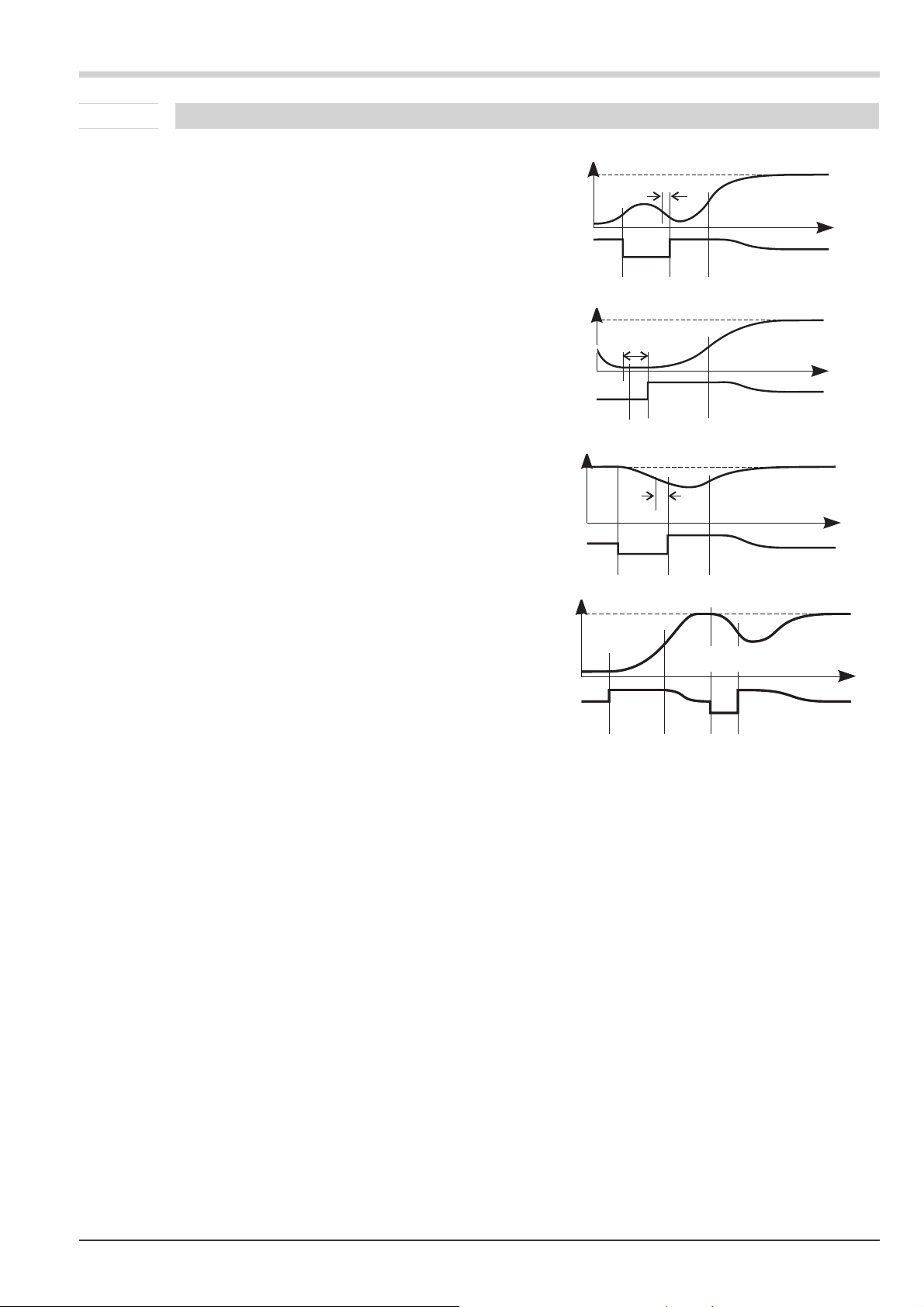
7.3.6 Examples for self-tuning attempts

.A.d.d.A.A

(controller inverse, heating or heating/cooling)

Start: heating power switched on

Heating power Y is switched off (1). When the change of process value X was constant during one minute (2), the power is switched on (3). At the reversal point, the self-tuning attempt is finished and the new parameter are used for controlling to setpoint SP.

Start: heating power switched off

The controoler waits until the process value has a con stant change of more than one minute. This possibly takes place already at start up (1). Heating power Y is switched on (2). At the reversal point, the self-tuning at tempt is finished and control to the setpoint is using the new parameters.

Start: at setpoint

Heating power Y is switched off (1). If the change of process value X was constant during one minute and the control deviation is > 10% of SP.Hi - SP.LO (2), the power is switched on (3). At the reversal point, the self-tuning attempt is finished, and control to setpoint SP is using the new parameters.

Three-point controller

The parameters for heating and cooling are determined in one attempt. The heating power is switched on (1). At reversal point 1, heating parameters Pb1, ti1, td1 and t1 are determined. The process value is lined out to the setpoint (2). The cooling power is switched on (3). At reversal point 2, parameters Pb2, ti2, td2 and t2 are determined and the self-tuning attempt is finished. Control to setpoint SP is using the new parameters.

Controlling

100%

Star t r

.A.A.d.d.A.A.

t Wendepunkt

reversal point

AdA

“ - “

100%

+100%

Y0%

-100%

Star t r

Start r

Star t r

.A.A.d.d.A.A.

t Wendepunkt

reversal point

AdA

t Wendepunkt 1

AdA

“ - “

t Wendepunkt

reversal point

AdA

“ -”

reversal point 1

. “ - “

t Wendepunkt 2

reversal point 2

KS 45 45 Self-tuning

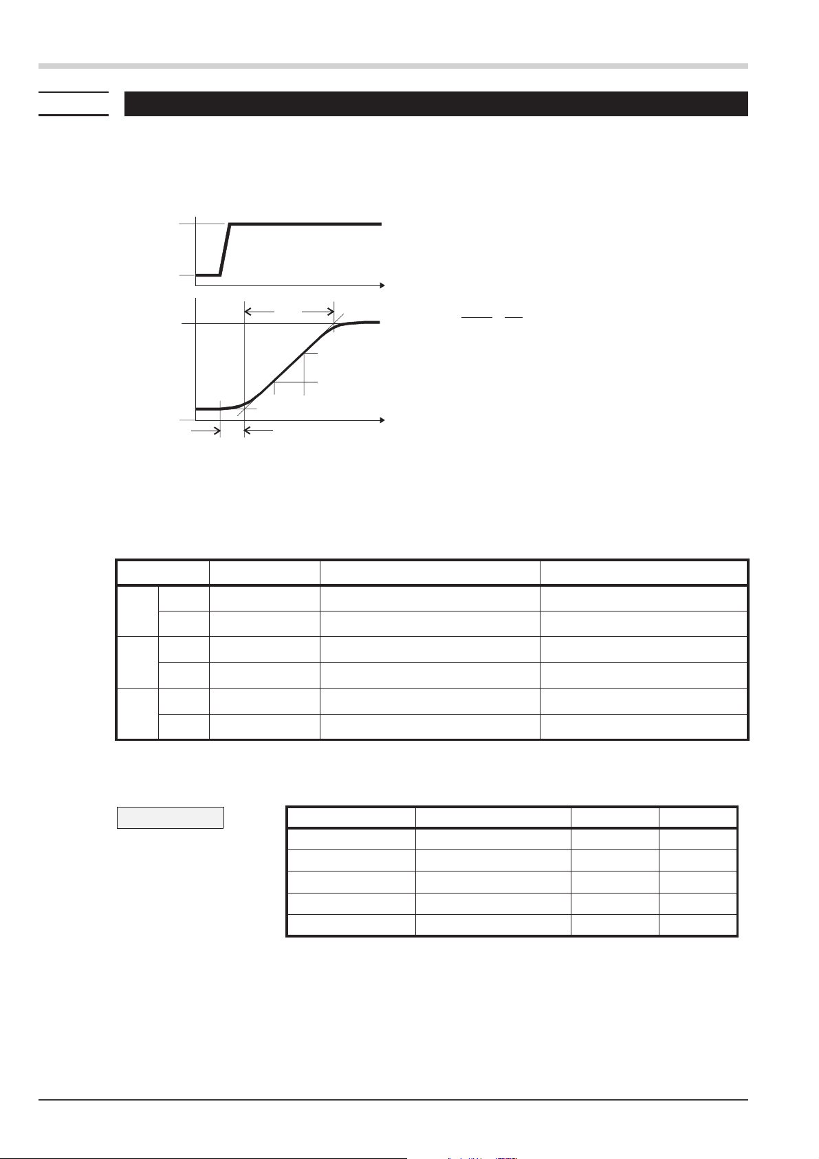
Controlling

7.4 Manual tuning

The optimization aid should be used with units on which the control parameters shall be set without self-tuning. For this, the response of process variable x after a step change of correcting variable y can be used . Frequently, plot ting the complete response curve (0 to 100%) is not possible, because the process must be kept within defined limits. Values T maximum rate of increase v

100%

max

and x

(step change from 0 to 100 %) or Dt and Dx (partial step response) can be used to determine the

max

y = correcting variable Y

= control range

Tu = delay time (s) Tg = recovery time (s)

= maximum process value

max

Xmax

{{x

The control parameters can be determined from the values calculated for delay time T v

, and characteristic K according to the formulas given below. Increase Pb1, if line-out to the setpoint oscillates.

max

max. rate of increase of process value

, maximum rate of increase

Parameter adjustment effects

Parameter Control Line-out of disturbances Start-up behaviour

Pb1 higher increased damping slower line-out slower reduction of duty cycle

lower reduced damping faster line-out faster reduction of duty cycle

td1 higher reduced damping faster response to disturbances faster reduction of duty cycle

lower increased damping slower response to disturbances slower reduction of duty cycle

ti1 higher increased damping slower line-out slower reduction of duty cycle

lower reduced damping faster line-out faster reduction of duty cycle

Formulas

K = Vmax w Tu controller behavior Pb1 [phy.units] td1 [s] ti1 [s]

PID 1,7 w K2w Tu 2 w Tu

With 2-point and 3-point con trollers, the cycle time must be adjusted to

t1 / t2 £ 0,25 * Tu

Manual tuning 46 KS 45

PD 0,5 w K Tu OFF PI 2,6 w K OFF 6 w Tu PKOFF OFF 3-point-stepping 1,7 w KTu2w Tu

8 Programmer

Programmer

SP,X

SP.01

SP.02

SP.03

SP.04

SP,X

Pt.01

Programmer set-up:

For using the controller as a programmer, select parameter SP.Fn = 1 in the ConF menu (r page 53). The pro grammer is started via digital inputs di1or the operating function Func. By selecting the appropriate parameter P.run =2/5,ConF-menu (r page 55), is defined which input is used for starting the programmer. If the end of the program shall appear as digital signal at one of the relay outputs, the appropriate parameter P.End = 1 must be selected for this output ( OUT.1...OUT.3, ConF-menu r page 58, 59).

Programmer parameter setting:

A programmer with 4 segments is available to the user. Determine a segment duration Pt.01 .. Pt.04 (in minutes) and a segment target set-point SP.01 .. SP.04 for each segment in the PArA menu. (r page 62).

Pt.02

Pt.03

Pt.04

Starting/stopping the programmer:

There are different possibilities for starting the programmer according to configuration:

Starting the programmer with a digital signal at the selected input di1.

•

If the Func-function is set as permanent display2 (selectable via BlueControl®), the program can be

•

started (on)with the È-key and stopped with Ì (OFF). If the Func-function was placed at the extended operating level, this element is selected with the ô -key. The function works as described above.

If the ProG-function is placed in display2 (selectable via BlueControl®), the program can be started

•

with the È-key (run), and stopped with the Ì-key (OFF). The ProG-function can also be placed in the extended operating level.

The ProG-function can also be used for displaying the programmerstatus.

If the ProG-function was selected, configuration P.run = 0 should be adjusted to avoid double operation.

The programmer calculates the setpoint gradient which shall reach the segment end setpoint out of segment end setpoint and segment time. This gradient is always effective. As the programmer starts the first segment at the real process value, the actual running time of the first segment can change (process value ¹ setpoint).

Starting conditions you'll find in the following drawing.

KS 45 47

Programmer

Process value = setpoint:

Programmer starts at the setpoint with the defined segment time

Process value between setpoint and

segmentend value SP.01 shortened segment duration.

Process value bigger/smaller than

SP.01; segment time 1 is skipped.

Process value bigger/smaller as the

setpoint: Program starts at segment start1.

After the program has elapsed the con

troller works with the latest tracking setpoint. The display shows the value End.

If the program is stopped whilst running (e.g. resetting the digital signal to di1), the programmer returns to the start point an waits for a new start signal. The de

vice goes to it's latest setpoint.

P, X

XSP.01?

SP<X<SP.01

X=SP

X<SP

SP,X

X>SP

X=SP

SP>X>SP.01

X<SP.01

start

Pstart

start

Pt.01

Pstart

Pt.01

Pstart

SP.01

Pt.02 Pt.03

SP.01

Pstart

Pt.02 Pt.03

SP.02

Program parameter changing while the program is running is possible.

Changing the segment time:

Changing the segment time leads to re-calculation of the required gradient. When the segment time has already elap sed, the new segment starts directly, whereby the set-point changes stepwise.

Changing the segment end setpoint:

Changing the set-point leads to re-calculation of the required gradient, in order to reach the new set-point during the segment rest time, whereby the polarity sign of the required gradient can change.

48 KS 45

9 Timer

9.1 Setting up the timer

9.1.1 Operating modes

6 different timer modes are available to the user. The relevant timer mode can be set via parameter SP.Fn in the Conf menu (r page 53).

Mode 1 (—)

After timer start, control is to the adjusted set-point . The timer (t.SP) runs as soon as the process value enters or leaves the band around the set-point (x = SP _ b.ti). After timer elapse, the controller returns to Y2. End and the output value are dis played alternately in the display line2.

IfY2=0isset, a switch off function of the outputs can be

realised

Mode 2 (····)

Mode 2 corresponds to mode1, except that control is continued with the relevant setpoint after timer (t.SP) elapse.

start

SP b.ti_

t.SP

Timer

End

Mode 3 (—)

After timer start, control is to the adjusted set-point. The timer (t.SP) starts immediately after switch-over. After timer elapsing the controller switches to Y2 and display 2 shows End alternately with the output value.

Mode 4 (····)

Mode 4 corresponds to mode 3, except that control is continued with the relevant set-point after timer (t.SP)elapse.

Mode 5 (delay)

The timer starts immediately. The controller output remains on Y2. After timer (t.SP) elapse, control starts with the adjusted set-point.

Mode 6

After set-point switch-over (SPr SP.2), control is to SP.2. The timer (t.SP) starts when the process value enters the adjusted band around the set-point (x = SP.2 _ b.ti). After time elapse the controller returns to SP. End and the set-point are dis played alternately in the lower display line.

start

SP.2b.ti_

t.SP

SP.2

End

SP SP

start

KS 45 49 Setting up the timer

t.SP

Timer

9.1.2 Tolerance band

Timer modes 1,2 and 6 are provided with a freely adjustable tolerance band. The tolerance band around the set-point can be adjusted via parameter b.ti in the Conf menu (x = SP.2 _ b.ti ) (r page 53)

9.1.3 Timer start

Various procedures for starting the timer are possible:

Y2 r Y switching via digital input di1 1 2xddddd- SP r SP.2 switching via digital input di1 1 x 2-----d

Power On 0 x ddddd-

Changing t.ti>0 (extended operating level) x x dddddd Serial interface (if provided) x x dddddd

Operation via BlueControl

Start via LOGI Mode

x 0-----d

(online operation) x x dddddd

SP.2=123456

when using a digital input, adjust parameter di.Fn = 2 ( ConF/ LOGI) ( key function)

x no effect

- not applicable

When using the digital input as a switch (di.Fn=0/1)orwhen using the Func switch-over function, the timer is re-started automatically after elapsing. Switch-over, e.g. opening, will cancel the timer function.

Using the Func function as a switch for starting the timer is not recommendable, because the timer would be re-started immediately after elapsing.

9.1.4 Signal end

If one of the relays shall switch after timer elapse, parameter TimE = 1 and inverse action O.Act = 1 must be selected for the relevant output OUT.1 … OUT.3 in the ConF menu (r page 57, 58). If direct action is selected, the relevant output signals the active timer.

9.2 Determining the timer run-time

The timer run-time can be determined via parameter t.SP in the PArA menu. The timer run-time must be specified in minutes with one digit behind the decimal point (0,1 minutes = 6 seconds). Alternatively, the timer run-time can be determined directly at extended operating level ( r chapter 9.3).

Determining the timer run-time 50 KS 45

9.3 Starting the timer

Dependent of configuration, the timer start is as follows:

at controller switch-on (power-on)

•

by adjusting the timer t.ti > 0 (at

•

extended operating level) by a positive edge at digital input di1 with

•

configured SP r SP.2 or Y2 r Y switch-over.

via the serial interface.

•

Timer

450.3

run

äüüü

g g

Display: the timer run is indicated by texts on LCD line 2,

which appear alternately with the other displays:

LCD-display 2 Signification

.r.u.n.

run

End

off • deletion of End display by pressing any key

With active timer, the time can be adjusted by changing parameter t.ti at extended operating level.

The status of an active timer can be output (Conf / Out.x / timE). A timer is set when started and reset by elapsing or cancelation.

timer is started

• timer is not running yet

•

timer is started

• timer is running

•

Timer elapsed

• Timer canceled

•

• timer is off

9.4 End / cancelation of the timer

The timer can be canceled. After elapse of the timer, the controller continues operating using the function dependent on operating mode.

Cancelation is possible by:

changing the timer setting t.ti = 0 (at extended operating level)

•

switching over digital input di1 (SP.2 r SP or Y r Y2 switch-over) configured as a push-button).

•

via the serial interface

•

If the digital input is defined as a switch or if the Func function with SP/SP2 or Y/Y2 switch-over is configured, the signal change will cancel the timer.

KS 45 51 Starting the timer

Timer

Mode

Behaviour after

1 display:

controller:

2 display:

controller:

3 display:

controller:

4 display:

controller:

5 * display:

controller:

6 Anzeige:

Regler:

elapse

End

none SP

End

Behaviour after

changing

t.ti =0

display: controller:

Anzeige: Regler:

none Y2

none SP

none Y2

none SP

keine SP

Cancelation

(before reaching

the timer band)

display: controller:

none Y2

- display: con

- display:

Anzeige: Regler:

keine SP

Cancelation

(after reaching the timer

band)

display: controller:

troller:

End

controller:

none

controller:

Anzeige: Regler:

End

Das Timersignal timEwird mit Start des Timers gesetzt, mit Ende oder Abbruch zurückgesetzt. * Der Timerstart erfolgt über Umschaltung Y2 r Y, der Timer schaltet auf Y2, beim Ende wird von Y2 r Y umgeschaltet.

End / cancelation of the timer 52 KS 45

10 Configuration level

10.1 Configuration survey

Dependent on the device version and further adjusted configurations, configurationdata can be hidden.

SP.Fn b.ti C.tYp C.Fnc mAn

C.Act

FAIL

rnG.L rnG.H

Inp.1

I.Fnc StYP 4wir S.Lin Corr In.F

Inp.2

I.Fnc StYP S.Lin Corr

In.F

Lim OUt.1 OUt.2

Fnc.1

Src.1

Fnc.2

Src.2 Fnc.3 Src.3

HC.AL LP.AL

0.Act Y.1 Y.2

Lim.1 Lim.2

Lim.3 LP.AL HC.AL HC.SC timE P.End FAi.1

FAi.2

0.Act

Y.1 Y.2

Lim.1 Lim.2 Lim.3 LP.AL

HC.AL HC.SC timE P.End FAi.1

FAi.2

OUt.3

O.tYP

0.Act Y.1 Y.2 Lim.1 Lim.2 Lim.3 LP.AL HC.AL HC.SC timE P.End

FAi.1

FAi.2

Out.0

Out.1

O.src

O.FAI

Configuration level

LOGI

di.Fn

L_r SP.2 SP.E

Y2 mAn

C.oFF Err.r P.run

I.ChG

othr

bAud Addr PrtY dELY

D.Unt

Unit

C.dEL

EndCntrc

End

g g

Adjustment:

The configuratiuons can be adjusted by means of keys ÈÌ .

•

Transition to the next configurationelement is by pressing key ô .

•

After the last configuration of a group, donE is displayed and followed by automatic change to the

•

next group

Return to the beginning of a group is by pressing the ô key for 3 sec.

Please check all interdependent parameters for their validity.

KS 45 53 Configuration survey

Configuration level

10.2 Configurations

Dependent on device version und adjusted configurations values not needed become hidden.

µ Entrys marked with this symbol are selectable only with existing device-option.

Controller Cntr

Name Value range Description

SP.Fn

b.ti

C.tYP

C.Fnc

mAn

C.Act

FAIL

rnG.L rnG.H

Adt0

setpoint processing

0 1 2 3 4 5 6 7 8 9

0...9999

0 1 2 3 4 5 6 7 8

0 1 2 3 4

0 1

0 1 2

0 automatische Optimierung 1 keine Optimierung

Setpoint/ ext. Setpoint program controller timer mode 1 timer mode 2 timer mode 3 timer mode 4 timer mode 5 timer mode 6 standard + SP-E programmer + SP.E

timer tolerance process value processing µ

process value = x1 ratio controller (x1+oFFS)/x2 difference (x1 - x2) max (x1, x2) min (x1, x2) mean value (x1, x2) Switch-over (x1, x2) Oxygen measurement with const. probe temperature Oxygen measurement with measured probe temperature

control behaviour

signaller (on/off controller) PID controller (2-point and continuous) D/Y switch-over 2 x PID (3-point and continuous) 3-point stepping controller

automatic/manual switching

Manual operation not permitted Manual operation admitted

direction of operation

inverse, e.g. heating direct, e.g. cooling

behaviour at sensor break

outputs off switch to Y2 mean correcting value

lower control range [phys] upper control range [phys]

Tuning of cycle time

Configurations 54 KS 45

Inputs InP.1 and InP.2

Name Value range Description

I.Fnc

S.tYP

4wir

S.Lin

Corr

In.F

fAI1

(fAI2)

0 1 2 4 6 7

0 1 2 3 4 5 6 7 8 9

10 Thermocouple type Typ B (0/100...1820°C), PtRh-Pt6%

18 20 21 22 23 24 25 26 30 31 40 41 42 43 44 45 46 47 50 51 52 53

0 1

0 1 2 3

OFF,

-1999...9999

0 1

function

no function heating current input External setpoint 2nd process value X2 no controller input process value X1

sensor type

Thermocouple type L (-100...900°C), Fe-CuNi DIN Thermocouple type J (-100...1200°C), Fe-CuNi Thermocouple type K (-100...1350°C), NiCr-Ni Thermocouple typeN (-100...1300°C), Nicrosil-Nisil Thermocouple type S (0...1760°C), PtRh-Pt10% Thermocouple type R (0...1760°C), PtRh-Pt13% Thermocouple type T (-200...400°C), Cu-CuNi Thermocouple type C (0...2315°C), W5%Re-W26%Re Thermocouple type D (0...2315°C), W3%Re-W25%Re Thermocouple type Typ E (-100...1000°C), NiCr-CuNi

special thermocouple (Linearization necessary) Pt100 (-200.0 ... 100,0 (150)°C) Pt100 (-200.0 ... 850,0 °C) Pt1000 (-200.0...850.0 °C) Special 0...4500 Ohm (default as KTY11-6) Special 0...450 Ohm Special 0...1600 Ohm Special 0...160 Ohm Current 0/4...20mA Current: 0...50 mA AC (HC input Inp2 only) Voltage 0...10V / 2...10 V (Inp1 only) Special (-2,5...115 mV) Special (-25...1150 mV) Special (-25...90 mV) Special (-500...500 mV) Special (-5...5 V) (Inp1 only) Special (-10...10 V) (Inp1 only) Special (-200..200 mV) Potentiometer 0...160 Ohm Potentiometer 0...450 Ohm Potentiometer 0...1600 Ohm Potentiometer 0...4500 Ohm

Resistance connection type(only for Inp.1)

3 wire connection 4 wire connection

linearization

no linearization special linearization

measured value correction

no correction offset correction 2-point correction scaling

alternative value INP

Forcing of analog input INP1, INP2 µ (only visible with BlueControlÒ!)

not active the value for this analog input is defined via interface.

Configuration level

KS 45 55 Configurations

Configuration level

Limits Lim1...Lim3

Name Value range Description

Fnc.1

(Fnc.2) (Fnc.3)

Src.1

(Src.2) (Src.3)

HC.AL

LP.AL

C.Std

C.Sch

0 1 2

0 1 2 3 4 6 7

0 1 2

0 1

OFF; 1 …

9999999

OFF; 1 …

9999999

function of limit 1 (2, 3)

switched off measurement value measurement value with latch

source of limit 1 (2, 3)

process value control deviation deviation + suppression INP1 INP2 Setpoint output value deviation + suppression without time limit

heating current alarm

switched off overload + short circuit break + short circuit

loop alarm

no LOOP alarm LOOP alarm active Control operating hours (only visible with BlueControlÒ!)

Control alternation number (only visible with BlueControl

Ò!)

Outputs Out.1, Out.2, Out.3,(relay/analog) µ

Name Value range Description

O.tYP

0 1 2 3 4 5

O.Act

0 1

Y.1

0 1

Y.2

0 1

Lim.1

0 1

Lim.2

0 1

Lim.3

0 1

LP.AL

0 1

HC.AL

0 1

type of OUT (only Out.3 - analog) µ

relay/logic 0 ... 20 mA continuous 4 ... 20 mA continuous 0 ... 10 V continuous 2 ... 10 V continuous transmitter supply

direction of operation

direct inverse

controller output Y1

not active active

controller output Y2

not active active

signal limit 1

not active active

signal limit 2

not active active

signal limit 3

not active active

loop alarm

not active active

heating current alarm

not active active

Configurations 56 KS 45

Name Value range Description

HC.SC

0 1

timE

0 1

P.End

0 1

FAi.1

0 1

FAi.2

0 1

Sb.ER

0 1

Out.0 Out.1

-1999...9999

O.Src

0 1 2 3 4 5 7 8

O.FAI

0 1

InF.1

InF.2

fOut forcing of the output (only visible with BlueControl

0 1

SSR short circuit

not active active

timer run

not active active

program end

not active active

signal INP1 fail

not active active

signal INP2 fail

not active active System bus error message µ nicht aktiv aktiv

scaling 0% (only for Out.3 analog) µ scaling 100% (only for Out.3 analog) µ signal source (only for Out.3 analog) µ

not active controller output y1 (cont.) controller output y2 (cont.) process value Effective setpoint control deviation INP1 INP2

fail behaviour µ

upscale downscale Status message for operating hours nicht aktiv aktiv Status message for number of switching cycles nicht aktiv aktiv

not active the value for this analog input is defined via interface.

Configuration level

Ò!)

Signal definition LOGI

Name Value range Description

di.Fn

0 1 2

L_r

0 1 2 5 7 8 9

KS 45 57 Configurations

function of inputs

direct inverse toggle key function

block front

(local/remote change Remote: front functions are blocked) interface only always on di1 switches Func switches Limit 1 switches Limit 2 switches Limit 3 switches

Configuration level

Name Value range Description

SP.2

0 2 5 7 8 9

SP.E

0 1 2 5 7 8 9

0 2 5 7 8 9

mAn

0 1 2 5 7 8 9

C.oFF

0 2 5 7 8 9

Err.r

0 2 7 8 9

P.run

0 2 5 7 8 9

I.ChG

0 2 7 8 9

fDI1 forcing of the digital input (only visible with BlueControlÒ!)

0 1

2nd setpoint

interface only di1 switches Func switches Limit 1 switches Limit 2 switches Limit 3 switches

external setpoint

interface only always on di1 switches Func switches Limit 1 switches Limit 2 switches Limit 3 switches

2nd actuator value

interface only di1 switches Func switches Limit 1 switches Limit 2 switches Limit 3 switches

automatic/manual switching

interface only always on di1 switches Func switches Limit 1 switches Limit 2 switches Limit 3 switches

controller off

interface only di1 switches Func switches Limit 1 switches Limit 2 switches Limit 3 switches

Reset error list

interface only di1 switches Limit 1 switches Limit 2 switches Limit 3 switches

program run/stop

interface only di1 switches Func switches Limit 1 switches Limit 2 switches Limit 3 switches switchover Inp1/ Inp2/ di1 interface only di1 switches Limit 1 switches Limit 2 switches Limit 3 switches

not active the value for this analog input is defined via interface.

Configurations 58 KS 45

Miscellaneous othr

Name Value range Description

bAud

Addr PrtY

dELY

S.IF

D.Unt

Unit

C.dEL

FrEq

0 1 2 3 4

1...247

0 1 2 3

0...200

0 1

0 1 2 3 4 5 6 7 8

9 10 11 12 13 14 15 16 17 18 19 20 21 22

0..200

baudrate µ

2400 Baud 4800 Baud 9600 Baud 19200 Baud 38400 Baud

address µ parity µ

No parity, 2 stop bits even parity odd parity No parity, 1 stop bit

response delay [ms] µ

system interface µ switched off switched on

display unit

no unit temperature unit (see Unit) O2 unit (see O2) % bar mbar Pa kPa psi l l/s l/min Ohm kOhm m0 A mA V mV kg g t Text of physical unit

parameter unit for O2 µ

Parameter in ppm with O2 function Parameter in % with O2 function

unit

no unit °C °F Kelvin

decimal points

0 digits behind the decimal point 1 digits behind the decimal point 2 digits behind the decimal point 3 digits behind the decimal point

modem delay [ms] Switch over 50/60 Hz (only visible with BlueControl

Netfrequency 50 Hz Netfrequency 60 Hz

Configuration level

KS 45 59 Configurations

Configuration level

Name Value range Description

ICof

0 1

IAda

0 1

ILat

0 1

IExo

0 1

Pass OFF...9999

IPar

0 1

ICnf

0 1

ICal

0 1

T.Dis2

Block controller off (only visible with BlueControl Released Blocked Block auto tuning (only visible with BlueControl Released Blocked Block error memory (only visible with BlueControl Released Blocked Block extended operating level (only visible with BlueControl Released Blocked

Password (only visible with BlueControl Block parameter level (only visible with BlueControl

Released Blocked Block configuration level (only visible with BlueControl Released Blocked Block calibration level (only visible with BlueControl Released Blocked Settings for text in display 2 (max. 5 digits) (only visible with BlueControl

Linearization Lin

only visible with BlueControlÒ!

Name Value range Description

U.LinT

0 1 2 3

In.1 … In.16 OFF (ab In.3)

Ou.1 … Ou.16

Depending on equipment version and the configuration unused parameters are hidden.

Value U.LinT defines the unit of input values specified for linearization of temperature values. Value entry in Celsius despite display of the measured value in Fahrenheit is possible.

Specify the input signals mV, V, mA, % or Ohm dependent on input type.

For special thermocouples (S.tYP = 18), specify the input values in mV and the output values in the

temperature unit adjusted in U.LinT. For special resistance thermometer (KTY 11-6) (S.tYP = 23), specify the input values in Ohm and

the output value in the temperature unit adjusted in U.LinT .

-1999...9999

-999.0 … 9999 output 1 … output 16

Temperature unit of the linearization table

without unit

in Celsius

in Fahrenheit

in Kelvin

input 1 … input 16

Configurations 60 KS 45

Resetting to factory setting (default)

r chapter 15.4

- preliminary - Parameter-level

11 Parameter-level

11.1 Parameter-survey

Dependent on device version und adjusted configurations values not needed become hidden. The data which can be operated via the front panel are shown below.

Cntr

Pb1 Pb2

ti1 ti2

td1 td2 t1 t2 SH d.SP tP tt

Y2 Y.Lo

SEtP

SP.LO SP.Hi SP.2 r.SP

t.SP

ProG

SP.01

Pt.01

SP.02

Pt.02

SP.03

Pt.03 SP.04

Pt.04

InP.1

InL.1 OuL.1 InH.1 OuH.1

t.F1 b.F1 E.tc1

InP.2

ôô

InL.2 OuL.2 InH.2 OuH.2

t.F2 b.F

b.F2

E.tc2

Lim

L.1

H.1

Hys.1 L.2 H.2

Hys.2 L.3

H.3

End

Hys.3 HC.A

Y.Hi Y.0 Ym.H L.Ym oFFS tEmP

Parameters can be adjusted with ÈÌ - keys.

•

Stepping to the next parameter by pressing the ô - key.

•

After the last parameter of a group donE appears in the display and the controller steps

•

automatically to the next group.

Stepping back to the beginning of a group is done by pressing the ô - key for 3 s. If, for 30 s no key is pressed, the controller returns to the operating level (Timeout = 30 s).

KS 45 61 Parameter-survey

Parameter-level

11.2 Parameters

µ Entrys marked with this symbol are selectable only with existing device-option.

Controller Cntr

Name Value range Description

Pb1 Pb2 ti1 ti2 td1 td2

t1 t2 SH

d.SP

tP tt

Y2 Y.Lo Y.Hi

Y.0 Ym.H L.Ym

oFFS tEmP

1...9999

1...9999 off, 1...9999 off, 1...9999 off, 1...9999 off, 1...9999

0,4...9999 0,4...9999

0..9999

-1999...9999

off, 0.1...9999

3...9999

-100...100

-105..105

-105...105

-100...100

1...9999

-120...120

0...9999

proportional band 1 [phys] proportional band 2 [phys] integral action 1 [s] integral action 2 [s] derivative action 1 [s] derivative action 2 [s] min. cycle time 1 [s] min. cycle time 2 [s] neutral zone [phys] additional contactD/Y[phys] min. pulse length [s] motor travel time [s] correcting variable 2 lower output range [%] upper output range [%] working point [%] max. mean value [%] max. deviation mean [phys] ratio offset probe temperature µ

Setpoint SEtP

Name Value range Description

SP.LO SP.Hi

SP.2 r.SP t.SP

-1999...9999

off,0.01...9999

0.0...9999

Programmer ProG

Name Value range Description

SP.01 Pt.01 SP.02 Pt.02 SP.03 Pt.03 SP.04 Pt.04

-1999...9999

0.0...9999

-1999...9999

0.0...9999

-1999...9999

0.0...9999

-1999...9999

0.0...9999

Inputs InP.1, InP.2

Name Value range Description

InL.1

-1999...9999

(Inl.2)

Oul.1

-1999...9999

(OuL.2)

InH.1

-1999...9999

(InH.2)

OuH.1

-1999...9999

(OuH.2)

lower setpoint range [phys] upper setpoint range [phys] 2nd setpoint [phys] setpoint ramp [/min] timer dwell time [min]

target setpoint 1 segment time 1 [min] target setpoint 2 segment time 2 [min] target setpoint 3 segment time 3 [min] target setpoint 4 segment time 4 [min]

lower input value [phys]

lower output value [phys]

upper input value [phys]

upper output value [phys]

Parameters 62 KS 45

Name Value range Description

t.F1

0...999,9

(t.F2)

E.tc1

OFF, 0...100

(E.tc2)

Limit Lim1...Lim3

Name Value range Description

L.1 H.1

HYS.1

L.2 H.2

HYS.2

L.3 H.3

HYS.3

HC.A

off, -1999...9999 off, -1999...9999

0...9999 off, -1999...9999 off, -1999...9999

0...9999

Parameter-level

filter time [s]

external TC[°C]

lower limit 1 [phys] upper limit 1 [phys] hysteresis 1 [phys] lower limit 2 [phys] upper limit 2 [phys] hysteresis 2 [phys] lower limit 3 [phys] upper limit 3 [phys] hysteresis 3 [phys] heat current limit [A]

Resetting to factory setting (default)

r chapter 15.4

KS 45 63 Parameters

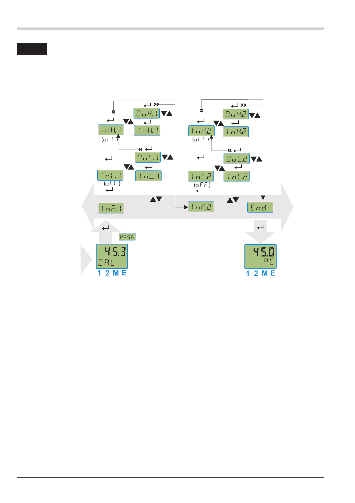
Calibrating-level

12 Calibrating-level

In the calibration menu ( CAL) the measured value can be adjusted.

The measured value correction ( CAL) is accessible only, if ConF / InP/ Corr = 1 or 2 was

selected.

Two methods are available

Offset - correction

•

2-point - correction

•

The InL.x and InH.x values are presented with one digit. As reference for the correcting calculation the full resolution is used.

Deleting the correction values is done fastest by switching off the measured value correction Corr = 0 or setting the scaling parameters to a linear behaviour.

The values InL.x and InH.x show the real measured value. The output values OuL.x and OuH.x start with the preset value.

64 KS 45

12.1 Offset-correction

The offset-correction shifts the input value by a pre-defined value. Parameter setting:

( ConF/ InP/ Corr =1 )

On-line offset correction at the process is possible.

display

OuL

OuLalt

Calibrating-level

standard

offset-correction

neu

450.3

450.0

äüüü

3sec.

PArA

ConF

CAL

InP

InL

OuL

End

InL: The actual input value of the scaling point is displayed.

The correction function is activated by means of keys ÈÌ ; the display changes from Off to the measured value.

The operator must wait, until the process is at rest. Subsequently, the input value has to be confirmed by pressing key ô .

OuL: The scaling point display value is indicated.

The operator can correct the display value by pressing keys ÈÌ. Subsequently, he presses key ô to confirm the display value.

KS 45 65 Offset-correction

Calibrating-level

12.2 2-point-correction

2-point correction can change the offset and gradient of the input curve. Parameter setting:

( ConF/ InP/ Corr = 2 ):

2-point correction is possible off-line by

means of an input signal simulator, or on-line in 2 steps: correct one value first

and the second value subsequently, e.g. after heating up the furnace..

450.3

450.0

äüüü

3sec.

PArA

ConF

CAL

InP

display

OuH

OuL OuLalt

alt

neu

InL

OuL

InL

standard

2-point-correction

InH

OuH

InL: The input value of the lower scaling point is displayed.

The correction function is activated via keys ÈÌ ; the display changes from Off to the measurement value.

Adjust the lower input value by means of an input signal simulator and press key ô to confirm the input value.

OuL: The display value of the lower scaling point is indicated.

Press keys ÈÌ to correct the lower display value and press key ô to confirm the display va lue.

InH: The input value of the second scaling point is displayed.

Activate the corrective function by pressing keys ÈÌ ; the display changes from Off to the measured value.

Adjust the upper input value by means of the input signal simulator and confirm the input value by pressing key ô .

OuH: The display value of the upper scaling point is indicated.

Correct the upper display value by pressing keys ÈÌ and press key ô to confirm the dis play value.

End

2-point-correction 66 KS 45

13 Engineering Tool BlueControl

The Engineering Tool BlueControlÒis the projecting environment for the BluePortâcontroller series as for the rail line family of PMA. The following 3 versions with graded functionality are available:

Functionality Mini Basic Expert

parameter and configuration setting yes yes yes download: transfer of an engineering to the controller yes yes yes online-mode / visualization SIM only yes yes defining an application specific linearization SIM only yes yes configuration in the extended operating level yes yes yes upload: reading an engineering from the controller SIM only yes yes basic diagnostic functions no no yes saving data file and engineering no yes yes printer function no yes yes online documentation, help yes yes yes implementation of measurement value correction yes yes yes data acquisition and trend display SIM only yes yes net- / multiple licence no nein yes wizard function yes yes yes extended simulation no no yes

Engineering Tool BlueControl

The mini version is - free of charge - at your disposal as download at PMA homepage www.pma-online.de or on the PMA-CD (please ask for).

At the end of the installation the licence number has to be stated or DEMO mode must be chosen.

At DEMO mode the licence num ber can be stated subsequently un der Help r

Licence r Change.

KS 45 67

Versions

14 Versions

Universalcontroller KS 45

1 universal input, 1 digital input with display and BluePort -interface

no plug-in connectors

with screw-terminal plug-in connectors

90...260V AC, 2 , INP2 as current input (0...20mA)

18...30VAC/18...31VDC, 2 , INP2 (0...20mA)

90...260V AC, mA/V/ logic + 2 , INP2 (0...20mA)

18...30VAC/18...31VDC, mA/V/ +2 , INP2 (0...20mA)

90..260V AC, 2 optocoupler output, 1 relay, INP2 as current input (0...20mA a.

0...50 mA AC)

18...30VAC/18..31VDC, 2 optocoupler output, 1 relay, INP2 as current input

(0...20mA u. 0...50 mA AC)

no option RS 485 / MODBUS - protocol

System interface (eng for 24V option)

di1 as contact input di1 as optocoupler input

INP2 as universal input, 0 -measurement,

di1 as

INP2

as universal input, 0 -measurement,

di1

as optocoupler input

standard

configuration to order

relay

as current input

contact input

S4 5 1

relay

logic relay

Accessories delivered with the controller:

Operating note

•

Rail-to-bus connector for

•

the interface option

Additional equipment with ordering data.

0 1

0 9

standard (CE-certified) certified to EN 14597 (replaces DIN 3440)

* not with optocoupler outputs (KS45-1x4... und KS45-1x5...)

cULus certified

Documentation

(please order the associated documentation)

operation manual KS 45 german 9499-040-71818 operation manual KS 45 english 9499-040-71811 interface description MODBUS rail line german 9499-040-72018 interface description MODBUS rail line english 9499-040-72011

Additional devices Order-No..

PC-adapter for BluePort® interface 9407-998-00001

BlueControl BlueControl

BlueControl

Mini german/english www.pma-online.de

with basic-licence rail line german/english 9407-999-12001

with expert-licence rail line german/english 9407-999-12011

68 KS 45

Technical data

15 Technical data

INPUTS

UNIVERSAL INPUT INP1

Resolution: >14 bits Decimal point: 0 to 3 decimals Digital input filter: adjustable 0.0...9,999 s Scanning cycle: 100 ms Linearization: 15 segments, adaptable with BlueControl® Measurement value

correction: Type: single-ended (except for thermocouples)

Thermocouples (Table 1)

Input resistance: ³1 MW Influence of source resistance: 1 µV/W Input circuit monitor: sensor break, polarity

Cold-junction compensation

• internal Typical additional error: ß_0.5K(ß 1.2 K max)

• external

- constant reference 0...100 °C

Break monitoring

Sensor current: ß1µA Operating sense: configurable

Resistance thermometer (Table 2)

Connection technology: 3 -wire, 4-wire (not at INP2-usage) Lead resistance: max. 30 W (for max. end of span)

2-point or offset

Measurement span

The BlueControl® software enables the internal characteristic curve for the KTY 11-6 temperature sensor to be adapted.

Physical measurement range: 0...4,500 W

Current and voltage measurement (Table 3)

Span start and span: anywhere within the measurement range

Scaling: freely selectable, –1,999...9,999 Input circuit 12,5% below span from 4...20mA / 2...10V Monitoring (current): start (2 mA)

O2measuring (option)

EMI measuring by means of INP1 (high-impedance mV inputs) suitable for probes with

constant sensor temperature (heated probes), setting by means

• of parameter measured sensor temperature (non-heated probes),

• measurement by means of INP2

ADDITIONAL INPUT INP2 (CURRENT)

Resolution: >14 bits Digital input filter: adjustable 0.0...9,999 s Scanning cycle: 100 ms Linearization: as for INP1 Measurement value correction: 2-point or offset Type: single-ended

Current measurement

Input resistance: approx. 49 W Span start and span: anywhere between 0 and 20 mA Scaling: freely selectable –1,999...9,999 Input circuit monitoring: 12,5% below span start (2 mA)

Input circuit monitoring: break and short circuit

Table 1 Thermocouple measurement ranges

thermocouple type measuring range error typ. resolution (Ô)

L Fe-CuNi (DIN) -100...900°C -148...1652°F ß 2 K 0,1 K J Fe-CuNi -100...1200°C -148...2192°F ß 2 K 0,1 K K NiCr-Ni -100...1350°C -148...2462°F ß 2 K 0,2 K

N Nicrosil/Nisil -100...1300°C -148...2372°F ß 2 K 0,2 K

S PtRh-Pt 10% 0...1760°C 32...3200°F ß 2 K 0,2 K R PtRh-Pt 13% 0...1760°C 32...3200°F ß 2 K 0,2 K

T** Cu-CuNi -200...400°C -328...752°F ß 2 K 0,05 K

C W5%Re-W26%Re 0...2315°C 32...4199°F ß 3 K 0,4 K D W3%Re-W25%Re 0...2315°C 32...4199°F ß 3 K 0,4 K E NiCr-CuNi -100...1000°C -148...1832°F ß 2 K 0,1 K

B* PtRh-Pt6% 0(100)...1820°C 32(212)...3308°F ß 3 K 0,4 K

special -25....75 mV ß 0,1 % 0,01 %

* Values for type B apply from 400°C upwards **Values apply from -80°C upwards

KS 45 69

Technical data

Table 2: Resistive inputs

type measuring current measuring range error typ. resolution (Ô) Pt100*** Pt100 -200...850°C -328...1562°F ß 1K Pt1000

KTY 11-6* -50...150°C -58...302°F ß 2 K 0,1 K

special special 0...450 [** Poti 0...160 [** Poti 0...450 [** Poti 0...1600 [** Poti 0...4500 [**

* Default setting is the characteristic for KTY 11-6 (-50...150°C) ** Including lead resistance *** up to 150°C at reduced lead resistance

Table 3: Current and voltage input

measuring range inpur resistance error typ. resolution (Ô)

0...20 mA 20 [ (voltage demand ß 2,5 V) £ 0,1 % 1,5 úA

0...10 Volt ~ 110 k [ £ 0,1 % 0,6 mV

-10...10 Volt ~ 110 k [ £ 0,1 % 1,2 mV

-5...5Volt ~ 110 k [ £ 0,1 % 0,6 mV

-2,5...115 mV* ? 1M[ £ 0,1 % 6 µV

-25...1150 mV* ? 1M[ £ 0,1 % 60 µV

-25...90 mV* ? 1M[ £ 0,1 % 8 µV

-500...500 mV* ? 1M[ £ 0,1 % 80 µV

-200...200 mV* ? 1M[ £ 0,1 % 420 µV

* for INP1: high-impedance, without break monitoring

for INP2: high-impedance, break monitoring always active

ß 0,25 mA

-200...100 (150) °C -328...212°F ß 1K 0,1 K

0,1 K

-200...850°C -328...1562°F ß 2K

0...4500 [**

ß 0,1 % ß 0,1 % ß 0,1 % ß 0,1 % ß 0,1 %

0,1 K

0,01 % 0,01 % 0,01 % 0,01 % 0,01 %

Heating current measurement

(via current transformer)

Input resistance: approx. 49 W Measurement span: 0...50 mA AC Scaling: freely selectable –1,999...9,999 A

ADDITIONAL INPUT INP2 (UNIVERSAL, OPTION)

Resolution: >14 bits Digital input filter: adjustable 0.0...9,999 s Scanning cycle: 100 ms Linearization: as for INP1 Measurement value correcti

on: Type: single-ended, exept

Thermocouples (Table 1)

Cold-junction compensation

•

internal,

- additional error: typ.: max.:

2-point or offset

thermocouples

ß_ 0,5 K ß -2,5 K

• external,

- constant setting 0...100 °C

Remaining technical data as for INP1

Resistance thermometer (Table 2)

Connection technology: 3-wire,

Remaining technical data as for INP1

Resistance measuring range

Remaining technical data as for INP1

Current and voltage measuring ranges

(Table 3)

Remaining technical data as for INP1 except

•

Voltage input ranges -10/0...10V, -5...5V are not possible.

•

Millivolt input ranges: high-impedance input for low-impedance sources

CONTROL INPUT DI1

Configurable as direct or inverse switch or push button!

Contact input

Connection of potential-free contact that is suitable for switching ‘dry’ circuits.

70 KS 45

Technical data

Switched voltage: 5 V Switched current: 1 mA

Optocoupler input

For active control signals.

Nominal voltage: 24 V DC, external supply Logic ‘0’: -3...5 V Logic ‘1’: 15...30 V Current demand: max. 6 mA

OUTPUTS

SURVEY OF OUTPUTS

* All logic signals can be ”OR-linked”.

RELAY OUTPUTS OUT1, OUT2, OUT3

Contact type: normally open * Max. contact rating: 500 VA, 250 V, 2A resistive load, 48...62 Hz, Min. contact rating: 6V, 1 mA DC Swithing cycles (elec

trical):

* Versions with two relays OUT1 & OUT2 have a common terminal.

for I= 1A/2A:

? 800.000 / 500.000

(at ~ 250V (resistive load))

Ripple (related to span end): 0...130kHz

Current output

0/4...20 mA, configurable, short-circuit proof.

Control range: -0.5...23 mA Load: ß700 W Load effect: ß 0.02% Resolution: ß 1.5 µA Error: ß 0.1%

Voltage output

0/2...10V, configurable, not permanently short-circuit proof

Control range: -0.15...11.5 V Load: ³ 2kW Load effect: ß 0.06% Resolution: ß 0.75 mV Error: ß 0.1% Additional error when ß 0.09%

OUT3 as transmitter supply

using simultaneously the current output Output: 22 mA / ³ 13VDC

OUT3 as logic signal

Load ß 700 W 0/ß 23 mA Load > 500 W 0/> 13 V

Note:

If the relays OUT1, 2 and 3 are used to operate external contactors, these must be fitted with RC snubber circuits to manufacturer specifications to prevent excessive voltage peaks at switch-off.

OPTOCOUPLER OUTPUTS OUT1, OUT2

(OPTIONAL)

Galvanically isolated optocoupler outputs. Grounded load: common ‘plus’ control voltage

Switch rating: 18...32 V DC; max. 70 mA Internal voltage drop: ß 1 V at Imax

Built-in protective circuits: for short circuit, wrong polarity

Note:

A protective diode for inductive loads must be fitted externally.

OUT3 UNIVERSAL OUTPUT

Galvanically isolated from the inputs. Parallel current/voltage output with common ‘minus’ terminal (combined use only in galvanically isolated circuits).

Freely scalable Resolution: 14 bits Tracking error I/U: ß 2% Residual ripple: ß_1%

KS 45 71

Technical data

Galvanic isolation

Version 1

system

RS 485

power

relay 1

relay 2

Version 2

system

RS 485

power

relay 3

safety isolation functional isolation

input

input 2

front interface

di 1 (contact)

di 1 (option

optocoupler

output 3

input 1

input 2 (HC)

front interface

di 1 (contact)

di 1 (option

optocoupler

optocoupler 1 optocoupler 2

AC supply

Voltage: 90...260 V AC Frequency: 48...62 Hz Consumption: approx. 7 VA max.

Universal supply 24 V UC

AC supply: 18...30 V AC Frequency: 48...62 Hz DC supply: 18...31 V DC Consumption: approx. 4 VA / 3W max.

* Instruments with optional system interface: energization is via the bus connector from field bus coupler or power supply module

Behaviour with power failure

Configuration and parameter settings:Permanent storage in EEPROM

BLUEPORT® FRONT INTERFACE

Connection to the controller front via a PC adapter (see ‘Additional Accessories’). The BlueControl configured, parameters set, and operated.

software enables the KS 45 to be

BUS INTERFACE (OPTIONAL)

RS 485

Connection via bus connector fitted in the top-hat rail. Screened cables should be used.

Galvanically isolated Type: RS 485

Transmission speed: 2,400, 4,800, 9,600, 19,200, 38,400

bits/sec Parity: even, odd, none Number of controllers per segment: Address range: 1...247

Galvanic isolation between inputs and outputs as well as from the supply voltage is provided.

Test voltages:

Between power supply and inputs/outputs: 2,3 kV AC, 1 min Between inputs and outputs: 500 V AC; 1min

Max. permissible voltages:

Between inputs/outputs against earth:

ß 33VAC

POWER SUPPLY

Depending on ordered version:

72 KS 45

Number of controllers per bus segment: 32

Protocol

MODBUS RTU

SYSTEM INTERFACE

For connection to field bus couplers (see system components) Connection via bus connector fitted in the top-hat rail.

ENVIRONMENTAL CONDITIONS

Protection mode

Front panel: IP 20 Housing: IP 20 Terminals: IP 20

Permissible temperatures

For specified accuracy: -10...55°C Warm-up time: < 20 minutes Temperature effect: ß 0,05%/10K add. influence to coldjunction compensation: Operating limits: -20...60°C Storage: -30...70°C

ß 0,05%/10K

Technical data

Screw terminals or spring-clamp terminals, both for lead

• cross-sections from 0.2 to 2.5 mm

Mounting method

Clip-on rail mounting (35 mm top-hat rail to EN 50 022). Locked by means of metal catch in housing base. Close-packed mounting possible.

Mounting position: vertical

Humidity

Max. 95%, 75% yearly average, no condensation

Shock and vibration

Vibration test Fc (DIN EN 60 068-2-6)

Frequency: 10...150 Hz Unit in operation: 1g or 0.075 mm Unit not in operation: 2g or 0.15 mm

Shock test Ea (DIN EN 60 068-2-27)

Shock: 15 g Duration: 11 ms

Electromagnetic compatibility

Meets EN 61326-1 for continuous, unattended operation.

Interference radiation:

• Within the limits for class B instruments. Immunity to interference:

Meets the test requirements for instruments in industrial areas. Criteria for evaluation:

• Surge interference partly has marked effects, which decay after the interference stops.

• With high levels of surge interference on 24V AC mains leads, it is possible that the device is reset.

With HF interference, effects up to 50 µV can occur.

Weight: 0.18 kg

Certifications

CE certified

Type tested to EN 14597 (replaces DIN 3440)

With certified sensors applicable for:

Heat generating plants with outflow temperatures up to 120°C

• to DIN 4751 Hot-water plants with outflow temperatures above 110°C to DIN

• 4752 Thermal transfer plants with organic transfer media to DIN

• 4754 Oil-heated plants to DIN 4755

•

cULus-certification

(Type 1, indoor use) File: E 208286

Standard accessories

• Operating instructions

• With ‘Interface’ option: bus connector for fitting into top-hat rail

GENERAL

Housing front

Material: Polyamide PA 6.6 Flammability class: VO (UL 94)

Connecting terminals

Material: Polyamide PA Flammability class: V2 (UL 94) for screw terminals

V0 (UL 94) for spring-clamp terminals and bus connector

Electrical safety

Complies with EN 61 010-1

Over-voltage category II Contamination degree 2 Protection class II

Electrical connections

Plug-in connector strips with choice of terminal type:

KS 45 73

Index

16 Index

0-9

2-point correction ...................66

Accessories ...................... 68

Additional equipment .................68

Analog output ..................30-31

Applications ......................5

Behaviour after supply v. on .............17

BlueControl ......................67

Dismounting ......................9

Filter .......................... 25

Forcing.........................31

Forcing of the inputs .................25

Front view ..................16,35-46

Functions .......................22

Input scaling ...................23-24

Input value monitoring ................27

Installation hints ...................15

Calibration (CAL)..................64

Cleaning ........................8

Configuration examples

- 2-point controller 38

- 3-point controller 39

- 3-point stepping controller 40

- Continuous controller 41

- D - Y -Off controller 42

- Signaller 37

Configuration level

- Configuration parameters 54 - 60

- Parameter survey 53

Configuration-level (

- Configuration-parameter 54 - 60

Connecting

Bus interface 12

di1 12

Inp1 11

Inp2 12

Out1, Out2 12

Out3 12

Connecting diagram..................11

Connection

Inp1 12

Inp2 12

Out1, Out2 12

Connectors ......................10

ConF)

Limit .......................27-29

Linearization......................60

Logic - output .....................31

Maintenance manager ..............32-33

Manual tuning.....................46

Number of switching cycles .............29

O2-measurement .................25-26

Offset-correction ...................65

Operating hours ....................29

Operating level ....................18

Operating structure ..................17

Operation .....................16-34

Parameter-level (PArA)

Parameter 62 - 63

Parameter-survey 61

Programmer

Changing segment end setpoint 48

Changing segment time 48

Parameter setting 47

Set-up 47

Starting/Stopping 47

74 KS 45

Safety hints .....................7-8

Self-tuning

Cancellation 44

Cancellation causes 44

Start 44

Set-point processing ...............35-36

Signaller........................37

Spare parts .......................8

TAG-No........................21

Terminal connections ..............11-12

Timer

Display run-LED 51

Operating modes 49

Signal end 50

Timer start 50

Timer-run-time 50

Timerstart 50

- Tolerance band 50

Transmitter power supply...............31

Index

Units..........................21

Versions ........................68

KS 45 75

Edition 06/2009 - Subject to change without notice - PMA_KS45_Rev02

West Control Solutions KS 45 User Manual

Specifications and Main Features

Frequently Asked Questions

User Manual