Wave Arts Power Suite 5 Users Manual

Download

Wave Arts

Power Suite 5

User Manual

Last updated: May 12, 2015

Table of Contents

1. Introduction .................................................................................... 5

1.1 Power Suite Overview .................................................................. 5

1.2 Installation ................................................................................. 5

1.3 Registration ............................................................................... 5

1.4 Wave Arts licensing using key codes .............................................. 6

1.5 Machine ID................................................................................. 6

1.6 PACE/iLok licensing ..................................................................... 7

1.7 Power Suite AAX ......................................................................... 8

1.8 Modifications for AAX DSP ............................................................ 8

1.9 Reduced configurations for AAX DSP .............................................. 9

1.10 Plug-in Instance Counts for AAX DSP .......................................... 10

2. Plug-in Control Operation ................................................................ 13

2.1 Knobs ....................................................................................... 13

2.2 Text Entry ................................................................................. 13

2.3 Selector button .......................................................................... 14

2.4 Sliders ...................................................................................... 15

2.5 Buttons .................................................................................... 15

2.6 Output Meters ........................................................................... 15

3. Menu Bar and Preset Manager .......................................................... 17

3.1 Bypass ..................................................................................... 17

3.2 Undo ........................................................................................ 17

3.3 Copy ........................................................................................ 17

3.4 A/B buffers ............................................................................... 17

3.5 Preset name and arrow controls ................................................... 18

3.6 Preset menu .............................................................................. 18

3.7 Factory Presets .......................................................................... 18

3.8 User Presets .............................................................................. 19

3.9 Save… ...................................................................................... 19

3.10 Import… .................................................................................. 19

3.11 Export… .................................................................................. 20

3.12 Reset… ................................................................................... 20

3.13 Tools menu ............................................................................. 20

3.14 About… ................................................................................... 20

3.15 Open User Manual… .................................................................. 21

3.16 Unlock Plug-in… ....................................................................... 21

3.17 Check for Updates… .................................................................. 21

3.18 Visit Website… ......................................................................... 22

4. TrackPlug ...................................................................................... 23

4.1 Overview .................................................................................. 23

4.2 About TrackPlug ......................................................................... 25

4.3 User Interface ........................................................................... 36

4.4 Parameters ............................................................................... 44

4.5 Parameter Descriptions ............................................................... 45

4.6 Specifications ............................................................................ 48

4.7 Presets ..................................................................................... 48

Wave Arts PowerSuite

5. MasterVerb .................................................................................... 53

5.1 Overview .................................................................................. 53

5.2 About MasterVerb ...................................................................... 54

5.3 User Interface ........................................................................... 58

5.4 Parameters ............................................................................... 61

5.5 Parameter Descriptions ............................................................... 62

5.6 Specifications ............................................................................ 65

5.7 Presets ..................................................................................... 65

6. FinalPlug ....................................................................................... 69

6.1 Overview .................................................................................. 69

6.2 About FinalPlug .......................................................................... 70

6.3 User Interface ........................................................................... 72

6.4 Parameters ............................................................................... 74

6.5 Parameter Descriptions ............................................................... 75

6.6 Specifications ............................................................................ 77

6.7 Presets ..................................................................................... 77

7. MultiDynamics ............................................................................... 79

7.1 Overview .................................................................................. 79

7.2 About Multiband Dynamics .......................................................... 80

7.3 User Interface ........................................................................... 82

7.4 Parameters ............................................................................... 85

7.5 Parameter Descriptions ............................................................... 86

7.6 Specifications ............................................................................ 88

7.7 Presets ..................................................................................... 88

8. Panorama ...................................................................................... 91

8.1 Overview .................................................................................. 91

8.2 About 3D Audio and Acoustic Environment Modeling ....................... 92

8.3 User Interface ......................................................................... 103

8.4 Parameters ............................................................................. 105

8.5 Parameter Descriptions ............................................................. 107

8.6 Specifications .......................................................................... 113

8.7 Presets ................................................................................... 113

License Agreement ........................................................................... 115

Support .......................................................................................... 117

Index ............................................................................................. 119



1. Introduction

1.1 Power Suite Overview

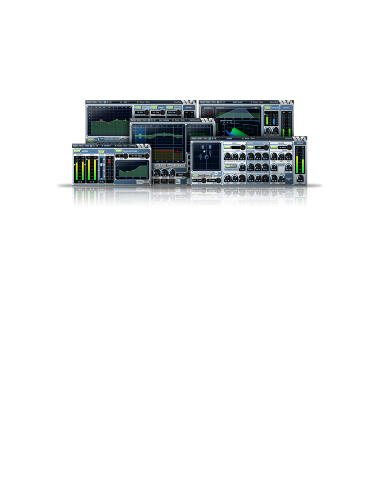
Power Suite is a set of plug-ins for mixing and mastering, consisting of the following individual plug-ins:

TrackPlug – channel strip with EQ and dynamics MasterVerb – stereo reverb FinalPlug – peak limiting and dither MultiDynamics – multi-band dynamics Panorama – spatial audio processor

1.2 Installation

Installers for Power Suite are found on the downloads page of the Wave Arts website. There are separate installers for Mac and Windows. You can download the full suite installer or individual plug-in installers. Mac installers are “.dmg” files which after downloading will expand into a “.pkg” installer file; double-click on the “.pkg” file to launch the installer. Windows installers are “.exe” files; double-click on the “.exe” file to launch the installer. The installers provide various options for selecting which plug-in formats to install and whether to use Pace/iLok or Wave Arts licensing for non-AAX formats.

There are also installers for AAX DSP formats. These should only be used if you have Pro Tools HDX hardware acceleration.

1.3 Registration

Wave Arts Power Suite

We support two licensing methods – Wave Arts licensing and PACE/iLok. When installing the plug-ins you must select which version of the plug-ins you wish to use. AAX format plug-ins always use PACE/iLok licensing. When you purchase a plug-in, you will be e-mailed a serial number (looks like WAPPP-XXXX-XXXX where PPP is a product code and X is a hex digit). Use the serial number to unlock the plug-in as described below.

1.4 Wave Arts licensing using key codes

Prior to registration, the plug-ins operate in demonstration mode; they are fully functional but stop operating after 30 days. To unlock the plug-in after purchasing, go to our Product Registration page, select “Wave Arts licensing” in the Licensing Method menu, and enter your serial number and your computer’s Machine ID (see Machine ID below). A key code (looks like XXXXXXXX) will be displayed and also e-mailed to you. Then, open the plug-in, select Unlock Plug-In from the Tools menu and enter your key code. You should see a message saying your registration was successful.

If you have purchased a plug-in suite, when you unlock any one of the plugins within the suite, the entire suite will be unlocked.

1.5 Machine ID

Your Machine ID is a unique 5-digit identification number our plug-ins generate based on properties of your computer. Our key code system uses the Machine ID and the product serial number to generate a key code that will unlock the plug-ins on your specific computer. The Machine ID is NOT used for PACE licenses (you will redeem a PACE code instead).

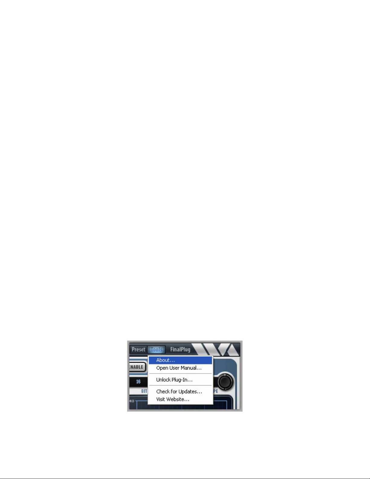
To find your Machine ID: Open the plug-in within a host application, click on the Tools button inside

the plug-in window and select the “About…” item:

1. Introduction

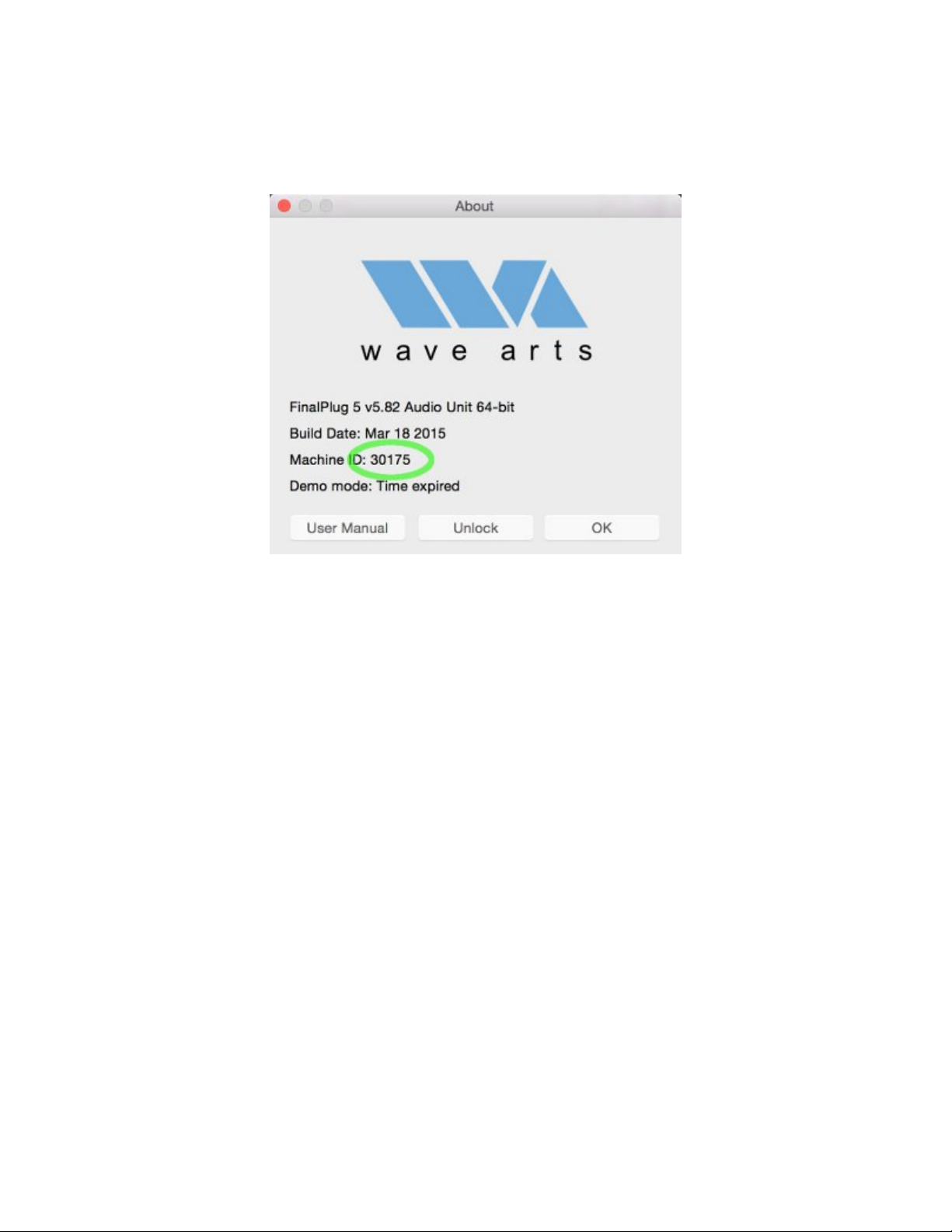
This will show the About box displaying information about your plug-in including the Machine ID, for example:

On Mac OS X and Windows systems, if your computer has Ethernet, the Machine ID is based on your hardware Ethernet MAC address. Therefore you should not have to re-register your plug-ins if you update your operating system or reformat your hard drive.

On Windows systems, changing the network configuration can sometimes result in your Machine ID changing. If this happens, you can get a keycode for the new Machine ID on our Register page and the plug-in should stay registered, even if your system alternates between Machine IDs. Contact us if you need further assistance such as additional keycodes.

1.6 PACE/iLok licensing

All our plug-ins support PACE/iLok. Prior to activation, the plug-ins will allow you to start a 14-day trial by creating an iLok account. To unlock the plug-in after purchasing, go to our Product Registration page, select “PACE/iLok”, and enter your serial number. A PACE redeem code (looks like XXXX-XXXXXXXX-XXXX-XXXX-XXXX-XXXX-XX) will be displayed and also emailed to you. There are two ways to redeem the code and generate a license. When opening the plug-in a dialog window will appear and give you the option to Activate the plug-in, you can paste the PACE redeem code there, and proceed to create or login to an iLok account and then transfer the license to an iLok or your machine. Otherwise, go to http://www.ilok.com, create an iLok account, and download and install the iLok License Manager. Within the

Wave Arts Power Suite

manager, under the Licenses menu, select “Redeem Activation Code” and paste your redeem code. Then transfer the license to either an iLok dongle or your machine. The plug-in will run only if it can find a license on an iLok or the machine.

When purchasing a plug-in suite, the redeem code will generate multiple licenses, one per plug-in in the suite, but the licenses are grouped together.

1.7 Power Suite AAX

The AAX format Power Suite plug-ins have some differences with their nonAAX counterparts. The next few sections will summarize the differences. Also, AAX specific differences are indicated in the detailed descriptions for each plug-in later in this manual.

Previous Power Suite plug-ins have been available in various native formats, including Avid’s RTAS and AS native formats, but also in AU, VST, DirectX, and MAS formats. Avid’s TDM format for operation on DSP cards was not supported.

The AAX (Avid Audio eXtensions) format replaces RTAS, AS, and TDM, and provides a single format for both native and DSP operation. Three of the Power Suite plug-ins support AAX DSP format for operation on DSP accelerated HDX hardware: TrackPlug, FinalPlug, and MultiDynamics. MasterVerb and Panorama have not been ported to AAX DSP and remain native only.

1.8 Modifications for AAX DSP

In order to port to AAX DSP, some modifications were made to the underlying algorithms.

 TrackPlug EQs now use new 32-bit filter architecture which performs

nearly as well at the 64-bit implementation previously used. This is done for efficient operation on 32-bit TI DSPs used in HDX hardware.

 The above mentioned 32-bit filter architecture is now used for

TrackPlug brickwall filters and MultiDynamics bandpass filters.

 The TrackPlug Real-Time Analyzer is operational only in AAX native.  The “Clean” dynamics processor in TrackPlug and MultiDynamics has

been jettisoned in favor of the superior “Vintage” processor.

 The Vintage dynamics processor has been slightly modified for

increased efficiency on the TI DSPs.

 MultiDynamics dynamics modes are now “Peak” and “RMS” (RMS mode

has been added).

1. Introduction

 Dynamics lookahead is maximum of 1 msec, for both TrackPlug and

MultiDynamics, due to limited memory on DSP.

 The limiting algorithm in FinalPlug has been rewritten for greater

efficiency on TI DSPs and has a new auto-release algorithm.

 The dither algorithm in FinalPlug is now 32-bits rather than 64-bits.

We believe the above changes were necessary to provide reasonable instance counts when running on DSP, without diminishing sound quality.

1.9 Reduced configurations for AAX DSP

Even with the above DSP optimizations, the full versions of TrackPlug, MultiDynamics, and FinalPlug use a considerable amount of CPU (and memory) on the HDX DSPs. This is because they were originally designed for native operation and have a large feature set. In typical native operation, many of these features may be disabled and will not consume any CPU. But on HDX DSP, we must allocate enough CPU for the worst case situation of all features enabled. For example, TrackPlug needs to allocate enough CPU to run all 10 bands of EQ, plus both brickwall filters, with all of the Gate, Comp1, and Comp2 dynamics enabled, all three running dual sidechain EQs, plus the Limiter. Because most users do not use all these features, it makes sense to provide feature reduced configurations that require less CPU (and memory) and thus can run more instances on HDX DSP.

The various configurations of the three plug-ins are summarized in the table below:

Plug-in Configuration Notes

TrackPlug TrackPlug Full version

TrackPlug E7GC 7-band EQ, Gate and Comp1 TrackPlug E7C 7-band EQ and Comp1

MultiDynamics MultiDynamics Full version, 6-bands

MultiDynamics 4-band 4 bands MultiDynamics 3-band 3 bands

FinalPlug FinalPlug Full version with dither

FinalPlug Limit Just limiter, no dither

TrackPlug comes with two feature reduced configurations. TrackPlug E7C provides 7 bands of EQ plus a single compressor (with optional sidechain EQ). The TrackPlug E7GC configuration provides 7 bands of EQ, a gate/expander, and a single compressor. Choosing 7 bands of EQ is motivated by the Avid D-control and D-command interfaces that have dedicated control layouts for 7 bands of EQ.

Wave Arts Power Suite

MultiDynamics comes with two feature reduced configurations consisting of 3-band and 4-band variations, as compared to the full implementation of 6bands.

FinalPlug comes with a limiter only configuration. This is because the dither section consumes considerably more CPU than the limiter but most users want only the limiter.

When running the reduced configurations, the same graphical user interface is shown, but certain user interface controls will be disabled if they control features not supported in the current configuration. The factory preset list is tailored to each specific configuration. User presets (via Wave Arts preset manager or Pro Tools preset manager) can be shared amongst all configurations of one plug-in, with the obvious caveat that not all features will be enabled or editable in the reduced feature configurations. Also, changing from one configuration to another may cause the settings to change. For example, when changing from the full 6-band MultiDynamics to 3-band and back to 6-band, only 3 bands will be enabled even if all 6 were originally enabled.

1.10 Plug-in Instance Counts for AAX DSP

The table below gives the maximum number of instances that will run on a single DSP chip for each plug-in configuration, at 48 kHz, 96 kHz, and 192 kHz sampling rates, for mono and stereo formats. These instance counts are valid as of the writing of this manual, future updates will likely increase instance counts as the plug-ins are further optimized.

Configuration Format 48 kHz 96 kHz 192 kHz

TrackPlug mono 3 3 2 stereo 3 3 1 TrackPlug E7GC mono 6 6 3 stereo 6 5 2 TrackPlug E7C mono 8 8 4 stereo 7 6 4 MultiDynamics mono 3 2 1 stereo 3 1 0 MultiDynamics 4-band mono 4 3 1 stereo 3 2 1 MultiDynamics 3-band mono 6 3 1 stereo 4 2 1 FinalPlug mono 8 4 2 stereo 4 2 1 FinalPlug Limit mono 18 18 15 stereo 17 17 8

1. Introduction

2. Plug-in Control Operation

2.1 Knobs

Please refer to the following guide for information about the various ways you can use knobs:

Function Mac

Increase/Decrease a parameter value (rotate clockwise/counterclockwise)

Fine adjustment — increase/decrease

Reset knob to default value

Click on the knob +

drag up/down

Shift + click + drag

up/down

PT: Command +

click

Command + click

-or-

Double-click

Click on the knob +

Right click + drag

Shift + click + drag

Windows

drag up/down

up/down

-or-

up/down

PT: Ctrl + click

Control + click

-or-

Double-click

PT: Option + click

PT: Alt + click

2.2 Text Entry

Many value displays are editable text. A text field is editable if your mouse cursor changes to an I-beam when moved over the text. Following is a table that fully describes how to use the text editing features:

Function Mac

Enter text entry mode Click in the display Click in the display Select text Click + drag Select entire text Double-click Delete character to left of cursor Delete character to right of cursor

Delete

Del

Windows

Click + drag Double-click

Backspace

Delete

Wave Arts Power Suite

Move the cursor left/right

Extend the current selection

Exit text entry mode

Select next parameter to edit Tab Select previous parameter to edit

Left/Right arrow

keys

Shift + click + drag

-or-

Shift + left/right

arrow keys

ESC*

-or-

Click outside value

box

-orTab

-or-

Return/Enter

Shift + Tab

Left/Right arrow

keys

Shift + click + drag

-or-

Shift + left/right

arrow keys

ESC*

-or-

Click outside value

-or-

Return/Enter

Shift + Tab

*Typing ESC causes the text to revert its original value before editing. You'll find that many parameters, such as frequency, will recognize units

typed into the text field. The following values, when typed into a frequency value box, are equivalent:

2k = 2 kHz = 2000 = 2000 Hz

box Tab

Tab

2.3 Selector button

The selector button cycles through a number of fixed values. Click on the button to go to the next value. Click on the text to display a pop-up menu of the available values. The table below describes the functionality of the selector button:

Function Mac

Go to next value Click on the knob Go to previous value Shift + click on knob Shift + click on knob Display pop-up menu of all choices

Click on text

Click on the knob

Windows

Click on text

2. Plug-in Control Operation

2.4 Sliders

Function Mac

Increase/Decrease a parameter value

Fine adjustment — increase/decrease

Click on the slider

handle + drag

Shift + click + drag

up/down

Click on the slider

Right click + drag

Shift + click + drag

Windows

handle + drag

up/down

-or-

up/down

Reset slider to default value

2.5 Buttons

Lighted buttons show a toggle state. A green, orange or yellow light indicates "on" and a black (extinguished) light indicates "off." Click the button to toggle the state.

Buttons that do not light up are used to activate certain commands.

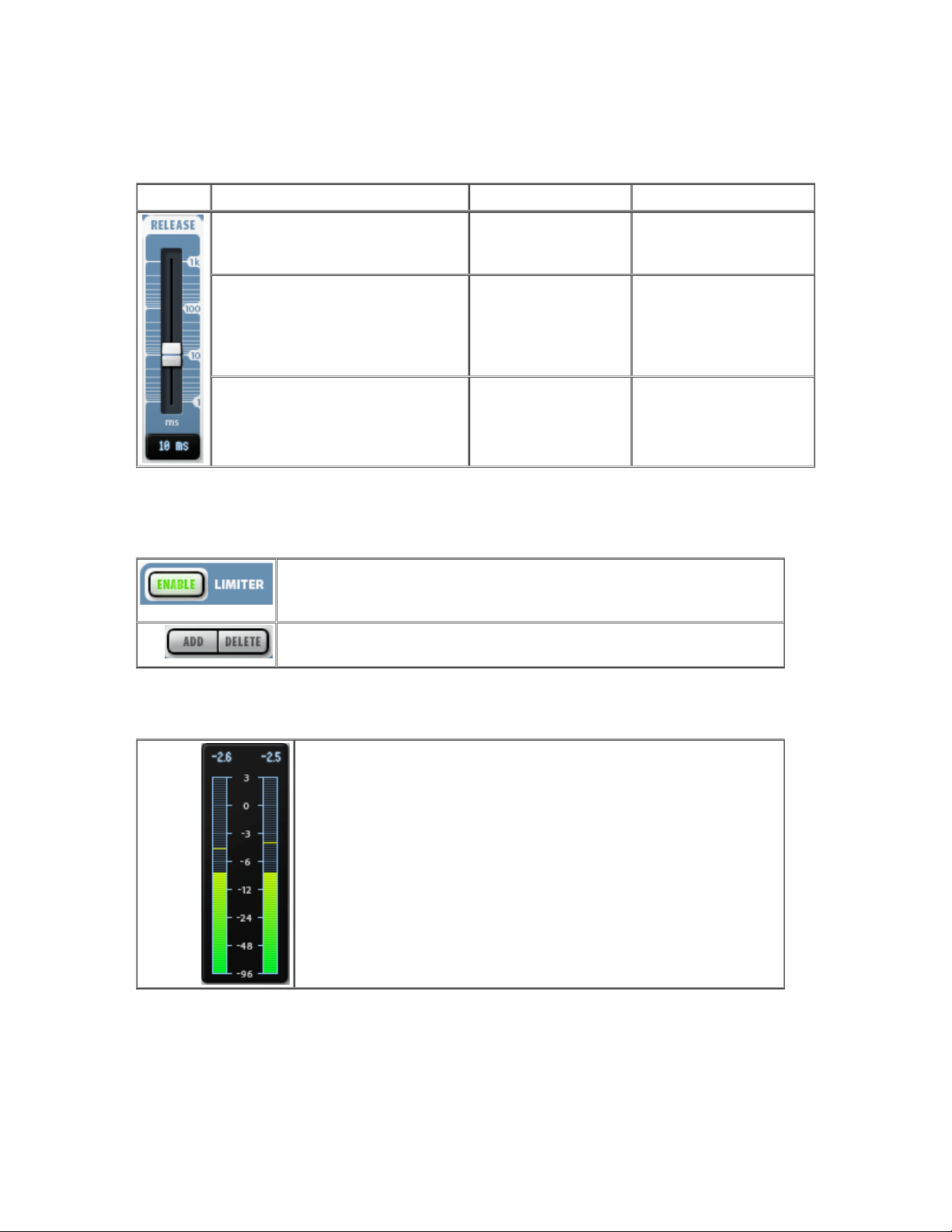
2.6 Output Meters

Output meters show the peak signal power in short time updates — in green from -96dB to -6dB, in yellow between 6dB and 0dB, and in red above 0dB. Peak hold levels are also drawn. The meter also stores the overall peak value for each channel, and displays these values in the peak indicator boxes above the meter. If the detector finds a peak value above 0dB, the text color will turn red as a warning. Click on either indicator box to reset them back to -96dB. Right click (PC) or Shift-click (Mac) on an indicator box to automatically increase or decrease the output gain so that the peak will be

-0.1dB.

Command + click

-or-

Double-click

Control + click

-or-

Double-click

3. Menu Bar and Preset Manager

All Wave Arts plug-ins in the Power Suite Bundle have the following menu bar displayed at the top of the plug-in:

This section describes the operation of the menu bar, preset manager, and the other functions available in the menus.

3.1 Bypass

Clicking on the bypass button bypasses the effect, that is, audio will pass through the effect without alteration. The button is lit when the effect is bypassed.

3.2 Undo

Clicking the Undo button causes the parameters to revert to their settings prior to the last edit. Only one level of undo is available, so clicking the undo button again will restore the parameters after the edit. Both A and B buffers (described below) have their own undo buffers.

3.3 Copy

Clicking the Copy button copies the current set of effect parameters to the unused A/B buffer. Hence, if the A buffer is currently selected, the parameters are copied to B, and if the B buffer is selected, the parameters are copied to A. After clicking Copy, you can continue to make changes, and then revert to the original copied settings by clicking either the A or B buttons to switch buffers.

3.4 A/B buffers

The A/B edit buffers allow you to compare two different sets of parameters or presets. One of the A or B buttons is always lit; the button that is lit shows the current buffer. Clicking either the A or B button will switch to using the other buffer, thus changing the effect settings (assuming different settings are stored in A and B).

Here’s how to use the A/B buffers to compare two different presets. Select a preset from the Preset menu, then switch to the other buffer and select a different preset. Now switch between the two buffers to alternate between the two different presets.

Wave Arts Power Suite

3.5 Preset name and arrow controls

The currently selected preset name is displayed in the text field in the menu bar. Changing any parameters causes an asterisk (*) to be displayed at the end of the name. This indicates that changes have been made to the preset. In order to save the changes to a user preset you must select the “Save…” item in the Preset menu, described below.

The arrow controls to the left and right of the preset name cycle through the set of factory and user presets. Clicking the right arrow goes to the next preset, clicking the left arrow goes to the previous preset.

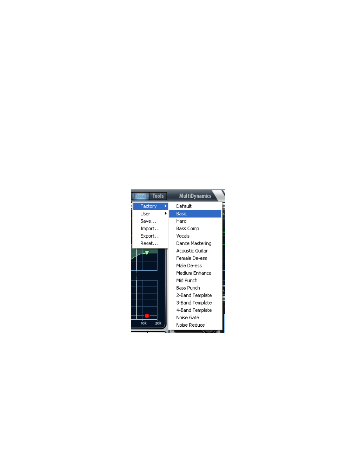
3.6 Preset menu

The Preset menu contains lists of factory and user presets for easy selection, and options for managing presets. The functions are described in the following sections.

3.7 Factory Presets

Factory presets are selected from a rolloff menu at the top of the Preset menu. Factory presets cannot be modified or deleted. The Default preset is always first in the list; it defines all default parameter settings.

For AAX DSP plug-ins which have reduced configurations, the same set of factory presets is presented for each configurat ion, even though the

3. Menu Bar and Preset Manager

configuration may not have all the features selected by the preset. For example, when loading a 6-band MultiDynamics preset into the 3-band configuration, the first three bands will be set up, while the top 3 bands from the preset are ignored. Similarly, when loading a TrackPlug preset into the TrackPlug E7GC configuration, only the first seven EQ bands, the gate, and Comp1 will be set up according to the preset.

3.8 User Presets

User presets are selected from a rolloff menu just below the Factory presets in the Preset menu. When you first run a Wave Arts plug-in, there will not be any user presets and the menu will be empty. When you save a preset using the “Save” option the preset is added to the User menu. All instances of a plug-in share the same set of user presets. So, after you save a preset with one instance of a plug-in, you can go to another instance and find that the preset can be found in its User preset menu too.

You can delete an individual user preset by holding down the SHIFT key while selecting the preset. The entire set of user presets can be deleted using the Reset option, described below.

User presets are stored in a text file called “<plugin> Presets.txt”, where <plugin> is the name of the plug-in you are using. If the file is deleted, an empty preset file will be created automatically the next time the plug-in runs. User presets files are stored in the following directory, depending on the operating system, where <username> is your Windows login name:

Mac OS-X: /Library/Application Support/Wave Arts/<plugin>/

Windows 7/8: C:/Users/<username>/AppData/Local/Wave Arts/

3.9 Save…

When you have created an effect you want to save as a preset, select the “Save…” option. You will be asked to name the preset and the preset will be saved in the set of User presets. If you supply the same name as an existing user preset, the preset will be overwritten with the new preset without any warning notice.

3.10 Import…

User presets can be written to files using the “Export” function, and read from files using the “Import” function. Selecting the “Import…” option will first ask if you want to replace or merge the imported presets. Replacing

Wave Arts Power Suite

causes your current set of user presets to be deleted and replaced with the presets read from the file, merging will add the presets read from the file to your set of User presets. Then you will be asked to choose a preset file for importing and the presets are read from the file.

Import can also be used to convert presets from an older version of the plugin to the current version. If the p lug-in detects presets from an older version and it knows how to convert them to the current version it will ask you if you want to convert the older presets to the current format.

3.11 Export…

Selecting the “Export…” option will first ask if you want to replace or merge the exported presets. Replacing causes the presets in the file to be deleted and replaced with the exported user presets, merging will add the user presets to the presets in the file. Then you will be asked to choose a preset file for exporting and the presets are written to the file.

Preset Export is also useful for making backup copies of your user presets. If you have a large set of user presets, be sure to export them to a backup file.

3.12 Reset…

Reset is used to delete all of your user presets. Selecting “Reset…” will first ask you if you really want to do this, and if you confirm, all the user presets are deleted.

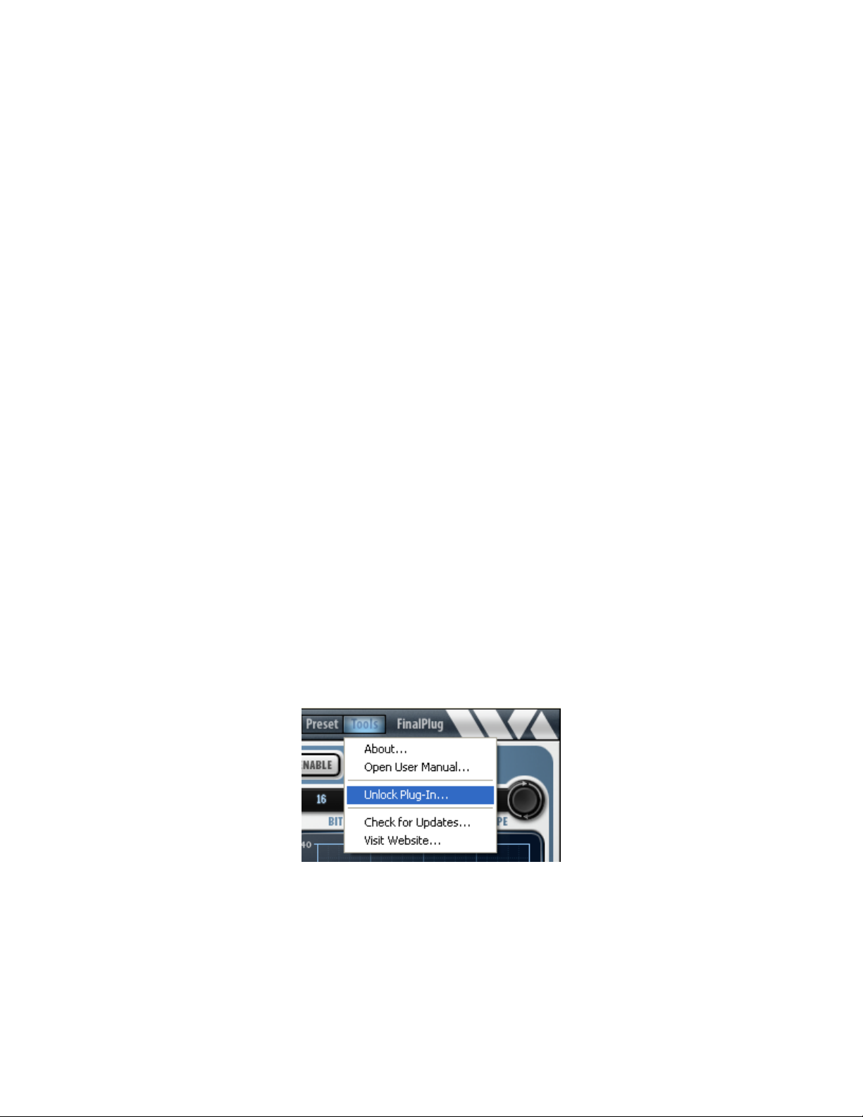
3.13 Tools menu

The Tools menu contains various important options, described below.

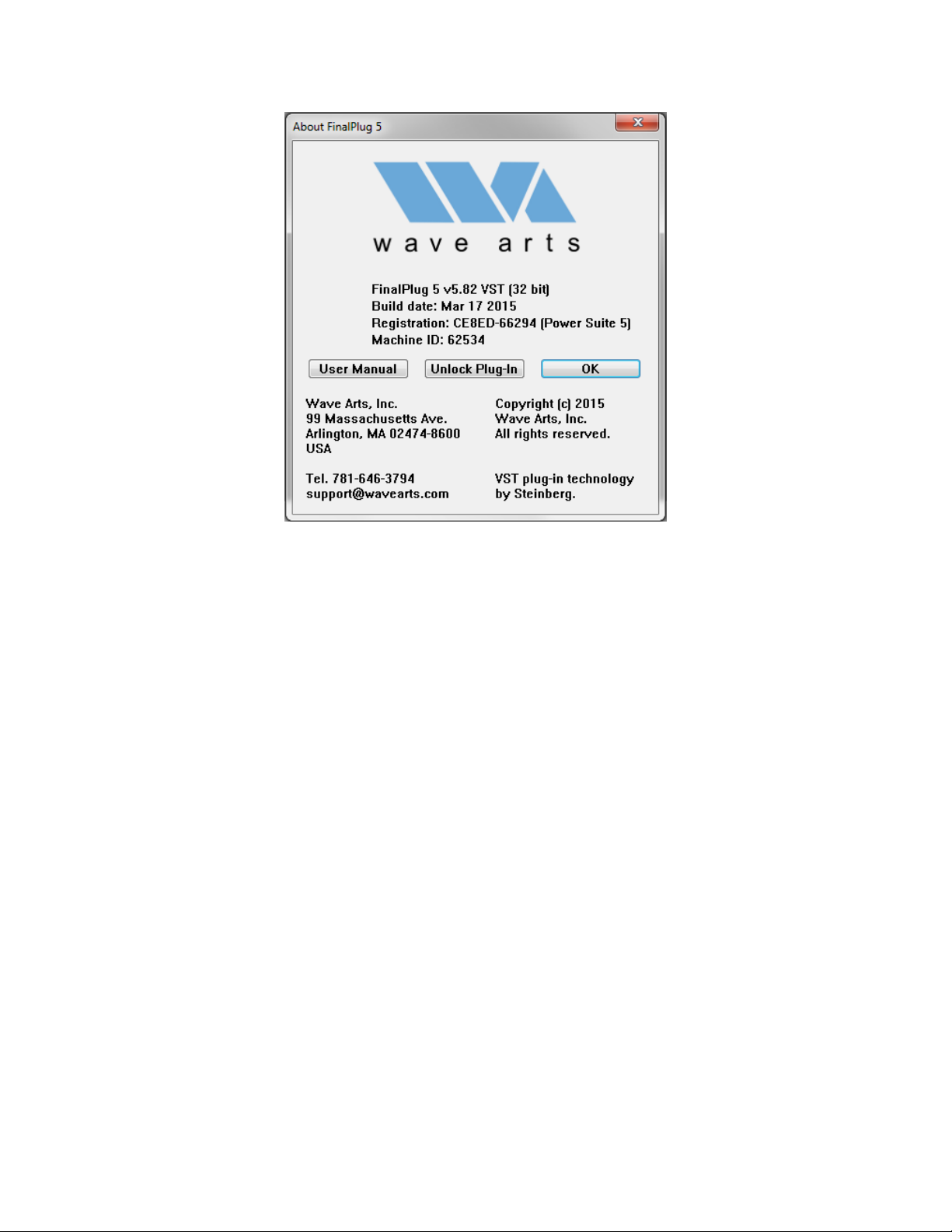
3.14 About…

The About option displays important information about your plug-in. An example is shown below:

3. Menu Bar and Preset Manager

On the top line, the plug-in name and version are displayed, along with the current plug-in format (AAX, DirectX, VST, AU, RTAS, or MAS). This is useful if you aren’t sure which format of the plug you are running. The build date of the plug-in is displayed on the next line. If the plug-in is using Wave Arts licensing, the registration status is displayed on the next line. If the plug-in is operating in demo mode, the time remaining (if any) is displayed. If the plug-in has been successfully registered (unlocked), the key code and bundle name is displayed. The Machine ID of the computer is displayed on the next line. Finally, buttons are provided for opening the registration dialog and the user manual. If the plug-in is using Pace/iLok licensing, there is no registration status or Machine ID displayed and the Unlock button will be disabled.

3.15 Open User Manual…

Select this option to open the user manual in a browser. If the manual isn’t found, you will be asked to navigate to it. Once the manual is opened successfully the plug-in remembers the location.

3.16 Unlock Plug-in…

This option is described in the Installation and Registration chapter of this manual.

3.17 Check for Updates…

Wave Arts Power Suite

If you are connected to the internet, selecting this option will launch a browser and will navigate to the Wave Arts Downloads page.

3.18 Visit Website…

If you are connected to the internet, selecting this option will launch a browser and will navigate to the Wave Arts home page.

4. TrackPlug

4.1 Overview

TrackPlug combines a 10-band EQ, a realtime analyzer, two compressors, a gate, a brickwall filter, and a lookahead peak limiter in one efficient, easy-to-use, and great sounding pro audio plug-in, ideal for tracking, mixing, and post production. Here are some of TrackPlug's key features:

 a 10-band EQ section with 11 different filter types  integrated realtime spectrum analyzer  low and high pass brickwall filters  two compressors and a gate, each with optional side-chain equalizer, variable

knees and optional lookahead delay

 choose between clean or vintage, peak or RMS dynamics modes  dual EQ comparison sidechain modes for precise de-essing, de-ploding  external sidechain inputs (AU, MAS, and RTAS only)  lookahead peak limiter  EQ routing pre or post dynamics  comprehensive metering  separate presets for each section  comprehensive set of factory presets designed by industry professionals  supports up to 192 kHz sampling rate

Wave Arts Power Suite

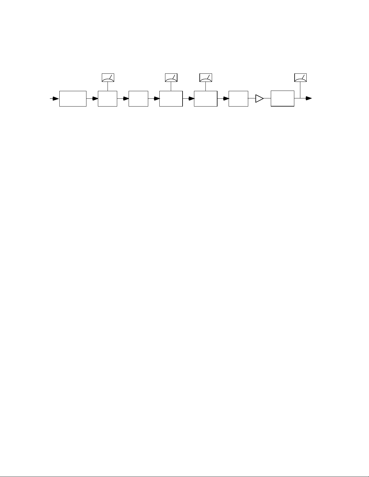
TrackPlug's audio routing and meter placement is shown in the diagram below:

Gate

Meter

Brickwall

filter

Gate

(pre)

TrackPlug audio routing diagram.

Comp1

Meter

Comp1 Comp2

Comp2

Meter

Output

Gain

(post)

Peak

Limiter

Output

Meter

Out

The input signal is processed first by the brickwall filter. This allows the user to eliminate noise signals that are outside the frequency range of the recorded instrument. Thumps, rumble and hum can be eliminated using a highpass brickwall, while high frequency hiss or tones can be eliminated using a lowpass brickwall.

The signal is processed next by the gate. The gate is commonly used to attenuate background noises when the main signal is not present. The gate can be used to reduce amplifier noise, microphone leakage, etc.

If the EQ routing is set to "pre", the EQ runs after the gate and before the compressors; if set to "post", it runs after the compressors. EQ is the principal tool to shape the tonal character of the sound.

The realtime spectrum analyzer runs either just befo re or after the EQ section depending on whether the RTA is set up to be pre or post EQ.

The two compressors run next. They can be configured in a variety of ways, from slow auto-gain control to faster compression, to aggressive distorting compression. The compressors can also be configured as de-essers or de-ploders by using the side-chain EQs.

If the EQ routing is set to "post", the EQ runs after the compressors. So me engineers prefer this configuration because they find that compression dulls the sound, requiring some EQ after compression.

The output gain and peak limiter run last. The peak limiter can be used as a hard compressor / loudness maximizer, by cranking up the output gain, or used simply to prevent peaks from exceeding -0.1 dB. This latter function is important for Pro Tools (RTAS format), because signals that exceed 0 dB are hard clipped and sound very distorted.

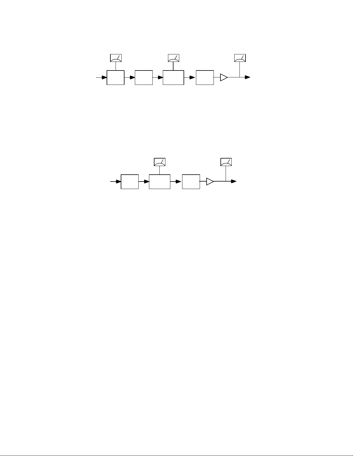
TrackPlug E7GC Configuration

For AAX DSP, the E7GC configuration provides a 7-band EQ, gate, and compressor. The audio routing is shown in the figure below.

4. TrackPlug

Gate

Meter

Gate

(pre)

Comp1

Meter

Comp1

Output

(post)

Output

Meter

Gain

Out

TrackPlug E7GC audio routing diagram.

TrackPlug E7C Configuration

For AAX DSP, the E7C configuration provides a 7-band EQ and compressor. The audio routing is shown in the figure below.

Comp1

Meter

Output

(pre)

Comp1

(post)

Output

Meter

Gain

Out

TrackPlug E7C audio routing diagram.

4.2 About TrackPlug

Brickwall filters

Brickwall filters are lowpass or highpass filters with very steep cutoffs, used to pass all frequencies up to the cutoff frequency and eliminate all frequencies beyond the cutoff. The frequency range that is passed unaltered is called the "passband", the frequency range that is attenuated is called the "stopband". TrackPlug's brickwall filters are implemented using 10th order elliptical filters, with at least 90 dB of stopband attenuation and less than 0.1 dB of passband ripple.

Brickwall filters are used to eliminate unwanted frequency ranges. Typically, a brickwall filter would be used when processing a noisy recording of an instrument sound that does not use the entire frequency range. The brickwall filter would be positioned at the edge of the instrument's frequency range to eliminate out-of-band noise. So for example, when processing voice, one could use the brickwall filters to eliminate all frequencies below 100 Hz and above 8 kHz.

The brickwall filters can also be used to zero in on a particular frequency range just for analysis purposes. For example, one could use the brickwall filters to listen to selected overtones in an organ, or to isolate the click of a kick drum.

Wave Arts Power Suite

Equalization

The equalizer is used to boost certain frequencies and reduce others, thus changing the tonality of a sound. When used in a mixing application, equalization is applied to each track so that it sits better in the mix. Generally, you want each instrument sound to be distinctly audible and sound natural, while maintaining a balanced mix. A good approach is to use as little EQ as possible, and when doing so, try to reduce frequencies rather than boost them, to give each track enough space in the mix. When equalization is used as a sound design tool, it can be applied aggressively to completely change the character of a sound.

It is helpful to have a general understanding of the frequency ranges in a mix: Low Bass (20 – 60 Hz)- controls rumble, this range is best reproduced on a

subwoofer equipped system. Bass (60 to 250 Hz)- the low end of the mix, where the fundamentals of bass and

other rhythm oriented instruments like the kick drum reside. Controls the overall fullness/roundness of a track or mix. Reducing around the 100 to 200 Hz range can help reduce “boominess”.

Low Midrange (250 to 2000 Hz)- many of the low harmonics of most instruments are in this range, and some boost here between 250 and 800 Hz can improve clarity of lower pitched instruments. Too much boost in this whole range can lend to a telephone-like quality (boost from 500Hz to 1Khz can sound horn-like, from 1Kz to 2Kz can sound tinny), and often frequencies in this area can be reduced on mid-range instruments like guitar, vocals and keyboards to improve a mix.

High Midrange (2000 Hz – 4000 Hz)- this range is an important speech recognition area, and also determines projection and clarity of mid-range instruments. Too much boost in this area can be fatiguing on the ear.

Presence (4000 Hz – 6000 Hz)- controls how close and distinct instruments and vocals sound, too much in this range will cause harshness.

Brilliance (6000 Hz – 20 kHz)- this range is associated with clarity, “sizzle”, and "air".

TrackPlug's equalizer provides up to 10 separate EQ bands, more than needed for most jobs. Each band has a choice of 11 different filter types per band. Again, we've erred on the side of providing more control rather than skimping. All of the filter types are based on second order filters; this limits their rolloff slope to -12 dB per octave. The filter types are described below.

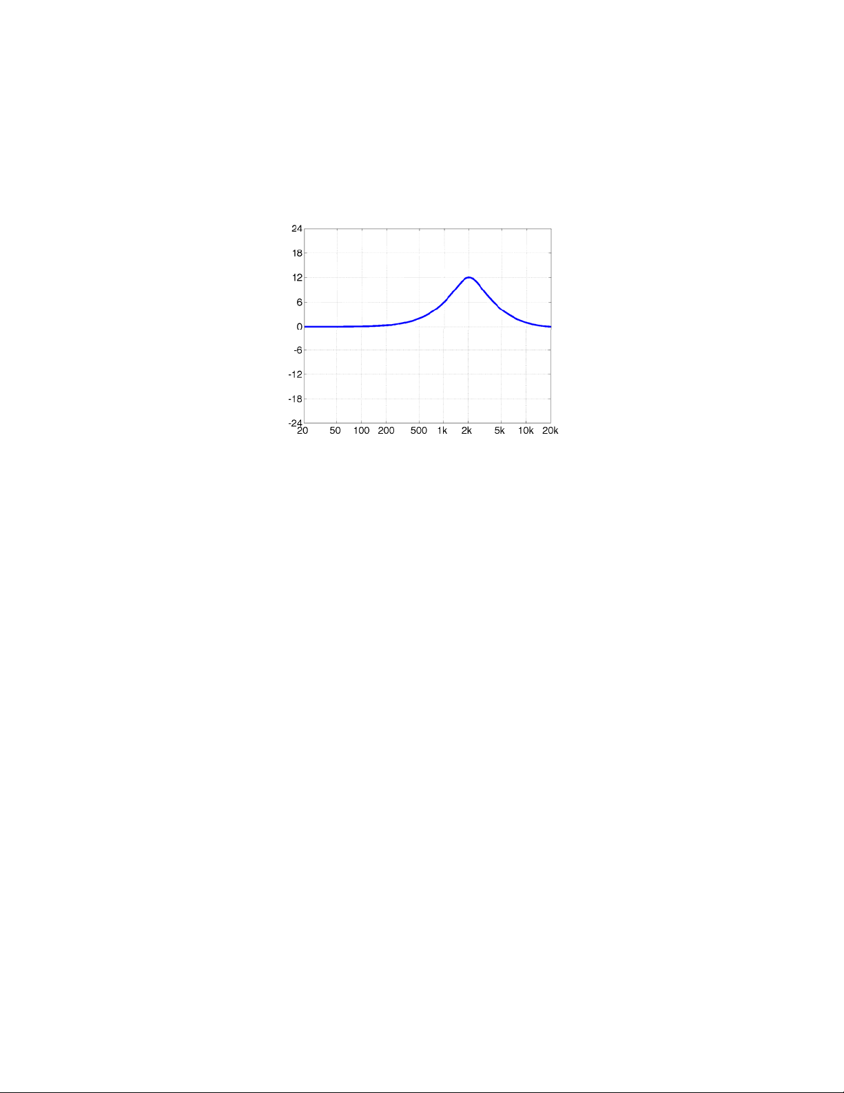
Parametric EQ

The parametric EQ type is one you will use often, as it allows you to reinforce or attenuate at a specific frequency point. The parametric EQ is defined in terms of the

4. TrackPlug

center frequency, the height of the boost/cut in dB, and the width. The width is measured in octaves between the half height points in the response. For example, if the center frequency is 2 kHz, the height is 12 dB, and the width is 2 octaves, then the width is defined at the 6 dB points in the response, which will be at 1 kHz and 4 kHz (one octave below and one octave above the center frequency, respectively).

Parametric EQ with freq = 2000 Hz, height = 12 dB, and width = 2 octaves.

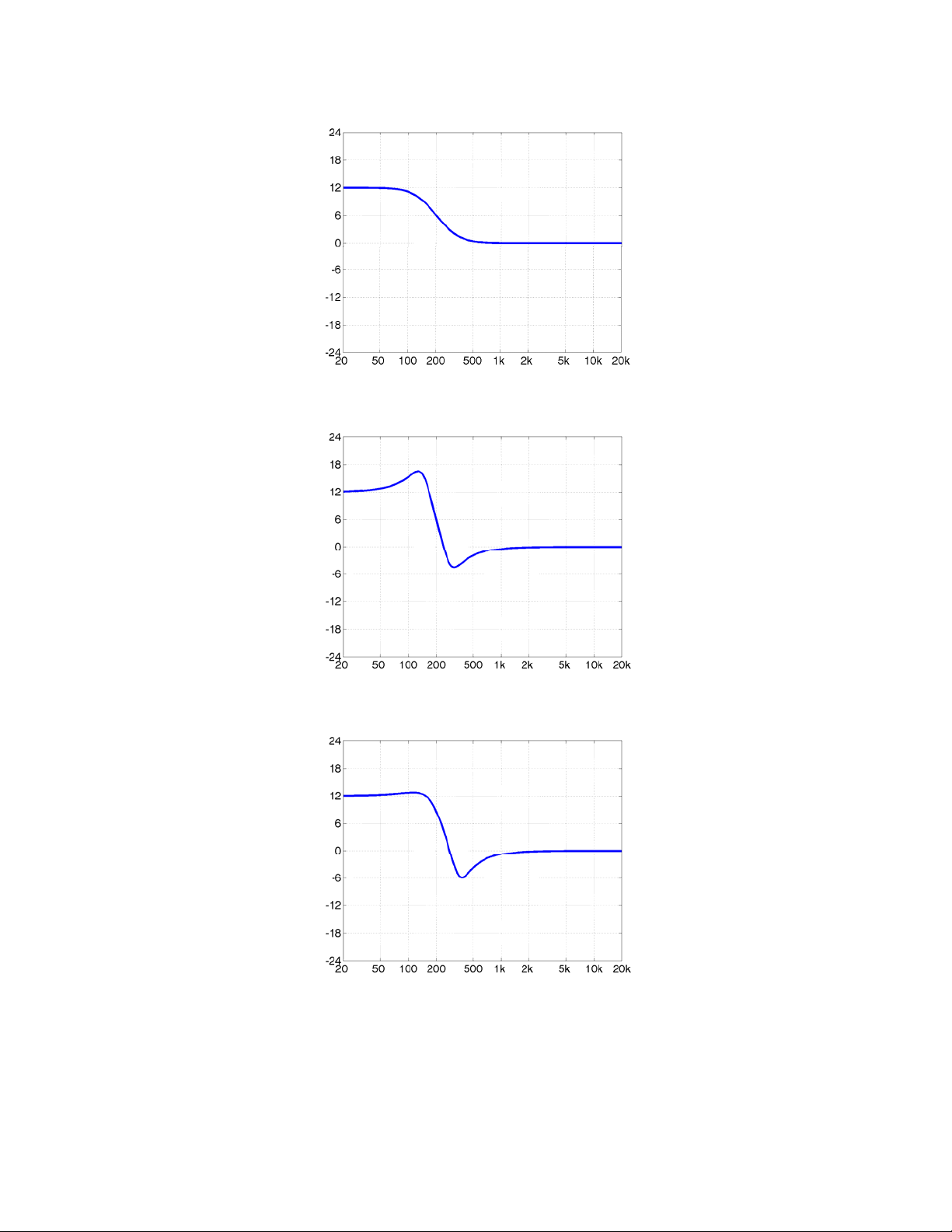
Shelf filter

The shelf filter boost or cuts by a fixed amount above or below a corner frequency. The shelf filter has parameters of corner frequency and shelf height in dB. The figure below shows a low shelf filter with a boost of 12 dB and a corner frequency of 200 Hz. The corner frequency is defined at the half height point in the response, so for example, in the figure below, the response is 6 dB at 200 Hz. TrackPlug provides three variations of the shelf filter which differ in the shape of the shelf transition: standard, resonant, and vintage. The standard shelf filter as shown in the figure has the steepest possible transition without having any overshoot. The "resonant" shelf filter has a variable transition slope defined by a resonance parameter. Filter resonances are usually defined using a Q parameter, called the "quality factor"; higher values of Q are more resonant and hence sharply tuned. TrackPlug uses the width knob to set the resonance, in units of Q. A shelf with a high resonance has a steep transition, but also overshoots symmetrically on each side, as shown in the figure below. The standard shelf filter is identical to the resonant shelf filter with a resonance (Q) of 0.707. Finally, the "vintage" shelf filter has a particular sort of as ymmetrical overshoot which is quite gentle and pleasing sounding. The vintage shelf is modeled after the response shapes of certain analog equalizers.

Wave Arts Power Suite

Low shelf with freq = 1000, height = 12 dB.

Resonant low shelf with freq = 200, height = 12 dB, Q = 2.

Vintage low shelf with freq = 200, height = 12 dB, Q = 1.414.

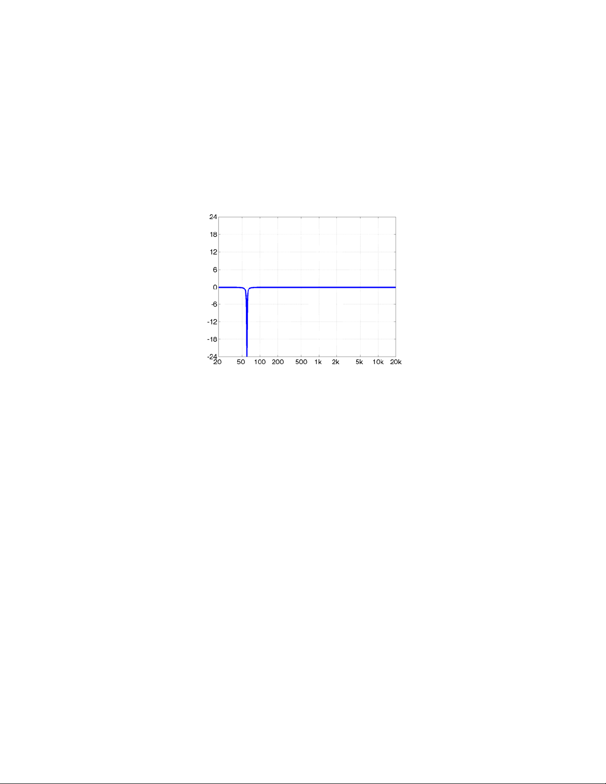
Notch filter

The notch filter cuts a specific frequency. It has parameters of center frequency and width. The width of the notch is measured in octaves between the -3 dB points of

4. TrackPlug

the filter response. TrackPlug's notch filter eliminates the center frequency completely, this would correspond to a height of minus infinity dB. The notch is commonly used to eliminate hum caused by power line interference. In the US, power lines oscillate at 60 Hz, in Europe and other parts of the world power lines oscillate at 50 Hz. Overtones of the hum are common and require an additional notch filter to cancel each overtone. Another commonly seen interference tone is caused by the horizontal flyback oscillation of televisions. In the US, NTSC TV sets oscillate at 15,734 Hz. In Europe, PAL and SECAM TV sets oscillate at 15,625 Hz. Often you will find these tones in acoustic recordings made anywhere near TV sets.

Notch filter with freq = 60, width = 0.1 octaves.

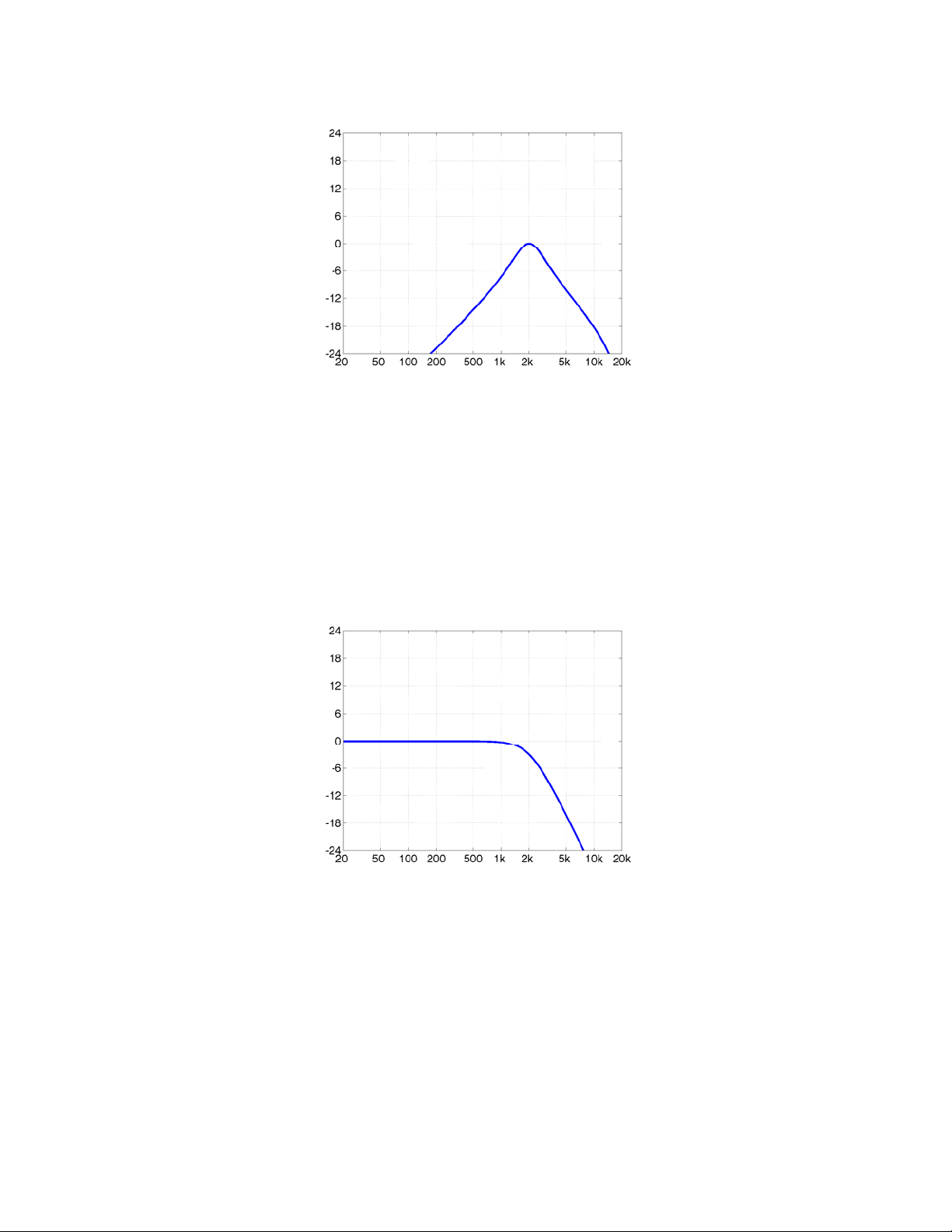
Bandpass filter

The bandpass filter is the opposite of the notch, it passes only the frequencies in a band around the center frequency. The bandpass filter has parameters of center frequency and width. The width of the bandpass is measured in octaves between the -3 dB points of the filter response. The bandpass filter would typically only be used in sound design to simulate the sound of a reduced frequency response, such as a telephone. One could also use the brickwall filters for this. The bandpass filter rolls off at -12 dB per octave on each side of the center frequency, much gentler than the brickwall, which rolls off at 60 dB/octave. The bandpass filter can also be used in analysis to isolate a particular frequency. For example, if there is a contaminating tone in a signal, one can sweep a narrow bandpass filter to isolate the tone, then switch to a notch filter to eliminate the tone.

Wave Arts Power Suite

Bandpass filter with freq = 2 kHz, width = 1 octave.

Lowpass and highpass filters

TrackPlug also provides lowpass and highpass filters. These pass frequencies up to a corner frequency, then roll off at -12 dB per octave beyond. The lowpass and highpass filters have only one parameter: corner frequency. The corner frequency is defined at the -3 dB point in the response. The choice to use the lowpass and highpass filters or to use the brickwall filters depends on how steep you need to rolloff to be.

Lowpass filter with freq = 2 kHz.

Real Time Analyzer (RTA)

TrackPlug has a built-in real time spectrum analyzer which allows you to see how the energy in the audio signal is distributed across frequencies. The RTA is not available when running AAX DSP format. The RTA displays the instantaneous energy in each of 31 frequency bands ranging from 20 Hz to 20 kHz. The width of each band is 1/3 octave which corresponds roughly to the critical bands in the human auditory system. Spectrum analysis is incredibly useful to see at a glance

4. TrackPlug

which frequencies make up a sound. The RTA can be inserted either before or after the EQ processing. Placing the RT A before EQ processing is useful to see the unaltered spectrum of the input signal. This can then guide subsequent application of EQ, perhaps to boost weak frequencies in the input, or attenuate strong frequencies. Placing the RTA after the EQ can then verify that the EQ has applied the intended adjustments. For stereo signals, the RTA displays the peak value for left and right channels in each band. The RTA will display a flat response with a pink noise input.

Dynamics

Dynamics processors are extremely useful and versatile tools. All dynamics processors work by tracking the level of the input signal and applying a gain in response to the input level. Compressors turn down the gain when the input exceeds a threshold level, whereas gates (expanders) turn down the gain when the input goes below a threshold. Compressors are often used to even out dynamics in a performance; making loud portions softer and making soft portions louder. When used more aggressively they can also add “punch” to a performance or to individual sounds, and when used really aggressively can add overtones and hence change the timbre of a sound. By combining a compressor with a side-chain equalizer, functions such as de-essing (reducing sibilant speech sounds) and de-ploding (reducing plosive speech sounds) can be done. Gates are typically used to squelch background noises in noisy recordings.

Threshold and Ratio

A compressor has five principal controls: threshold, ratio, attack time, release time, and makeup gain. The threshold is the input level at which compression will kick in. The ratio parameter determines how much gain reduction will be applied as the input exceeds the threshold. The definition is somewhat archaic and confusing. The range of ratios is 1 to infinity. A ratio of 1 means no gain reduction, while a ratio of infinity means the gain reduction is equal to the amount the input exceeds the threshold (hence the input will be pinned at the threshold value). In general, for a ratio R, the gain reduction is (R-1)/R of the amount the input exceeds the threshold. So to take a typical example, if the input is 12 dB over threshold with a ratio of 3, the gain reduction will be 8 dB.

But compressors are not really about decreasing gain, they are really about increasing gain. What they do is decrease the peaks in a signal so the rest of the signal can be boosted. This is what the makeup gain control does, it applies a constant gain boost to increase the soft parts of a signal while the compressor dynamically pushes down the peaks.

Attack and Release Time

The attack time and release time parameters are really important. The attack time controls how fast the gain is turned down when gain reduction is to be applied and

Wave Arts Power Suite

the release time controls how fast the gain is turned back up. Consider the example of compressing a drum hit. With a small (fast) attack time, the initial transient of the drum hit will be compressed because as soon as the transient exceeds the threshold the gain reduction kicks in immediately. As you increase the attack time, it takes longer for the gain reduction to fade in and the initial transient of the drum hit passes through uncompressed. So in this case, when you want to hear more drum attack, you increase the attack time. After the transient has passed and the drum sound begins its decay, the compressor will begin releasing, increasing the gain back to the nominal level as set by the makeup gain. A short release will restore gain immediately, in which case the drum sound will have essentially the same decay it had originally. A longer release time will restore gain more slowly, thus increasing the decay ti me of the original drum sound. So the original “BUMPH” of the drum sound becomes “BOOOOMMMMPH” after compressing. That’s punch. The ability to change the decay time of acoustic instruments after they have been recorded is a really powerful capability of compressors.

When gating, the attack and release time parameters are reversed. The release time controls low fast the gain is turned down and the attack time controls how fast the gain is restored. Consider the example of a drum recording containing background noise, assuming the threshold has been set just above the background noise and the ratio is large. When the signal goes below threshold the gate kicks in and begins reducing gain. A short release time will decrease gain rapidly, abruptly cutting off the decay of the drum. Longer release times cause the gain to decrease more slowly, which may sound more natural but also allow the noise to be audible at the end of the decay. On the next d rum hit, the gate will restore gain according to the attack time. Using a short attack time is prudent in this case, otherwise the attack of the drum will be lost due to the slow attack fade-in of the gate. So, when gating, the attack and release times correspond to the attack and release times of the instrument you are processing.

Peak and RMS modes

Dynamics processors often have peak and RMS modes. In peak mode, the processor is tracking the peak levels in the signal, that is, looking at the peak absolute values of the signal. In RMS mode, the processor is tracking the RMS levels of the signal. RMS stands for “root mean square”, it essentially means you square the signal, take the average value, and take the square root of this value. This is a measure of the average power level of the signal, which correlates roughly with the perceived loudness of the signal. In practice, computing a running estimate of the RMS level requires doing a short term average of the recent input, hence the RMS levels change much slower than the peak levels. Furthermore, peak levels will tend to be much higher than RMS levels. The relationship between peak and RMS levels depends on the signal. A square wave or a constant (DC) signal will have identical peak and RMS values. A sinusoid (pure tone) has a peak that is 3 dB higher than its RMS value. For many music and speech signals, the peak values may be 10 dB higher than the RMS levels. One would typically use peak mode compression when processing an instrument sound, or aggressively compressing a mix, whereas RMS mode would typically be used to even out the loudness of mix.

4. TrackPlug

TrackPlug dynamics modes

TrackPlug has three dynamics processors: a gate and two compressors. Each compressor has 5 modes: Clean Peak, Clean RMS, Vintage Peak, Vintage RMS, and Vintage Warm, while the gate is limited to using one of the two Clean modes.

AAX format has a different selection for dynamics modes. Each processor has 3 modes: Peak, RMS, and Warm, while the gate is limited to using either Peak or RMS mode. These modes correspond the to the “Vintage” modes in non-AAX versions of TrackPlug; for AAX, the so-called “Clean” modes have been omitted.

The clean modes are inherited from earlier versions of TrackPlug; they prevent harmonic distortion when processing tonal sounds, even when using fast attack/release times. Consider how a traditional compressor responds to a sinusoidal waveform: it will attack on the peaks and release during the troughs, essentially shaping the sinusoid into a square wave and adding odd harmonic distortion. In contrast, the TrackPlug clean processor estimates the signal level once after each complete waveform, hence the clean mode sees a sinusoidal input as having a purely constant amplitude. Thus, the clean compressor (and clean gate) will not shape each waveform.

The clean modes are indispensable for gating. They prevent any waveform distortion as the gate is turning on or off. The gate is limited to only using the two clean modes. The clean modes are also useful when you are compressing aggressively but you want to preserve attack transients (say for a kick drum for example) or if you want to prevent any harmonic distortion during constant level tonal sections.

When we refer to aggressive compression settings, we primarily mean using fast attack and release times (say 0.1 to 5 msec), which are fast enough to cause the compressor to reattack with every period of the incoming signal. This in turn causes waveform shaping and the production of harmonic overtones. When using long attack and release times the gain changes are spread over many periods of the signal and distortion is substantially reduced. Using large ratios and hard knees also contributes to aggressive compression.

The vintage modes work like traditional compressors. If you select aggressive compression settings, the vintage modes will distort. The vintage modes include Vintage Peak, Vintage RMS, and Vintage Warm. The Vintage Peak mode detects the peak absolute value of the input signal; the resulting compression will affect the positive and negative swings of the signal equally, and will thus create odd harmonic overtones. The Vintage RMS mode computes the squared input signal and runs this through an averaging envelope follower. Because of the relatively slow averaging used to obtain the RMS level compared to the very fast peak level detection, using fast attack and release times will produce less distortion with Vintage RMS mode than with Vintage Peak mode. However, like Vintage Peak mode, Vintage RMS mode also produces only odd harmonic overtones. Vintage Warm mode is like Vintage Peak mode, but only the positive peaks of the input

Wave Arts Power Suite

signal are detected (using a half-wave rectifier). Thus the positive and negative swings of the signal are processed differently, and this causes the production of both even and odd harmonic overtones. With aggressive compression settings, the difference in tonal character between the three Vintage modes is striking.

TrackPlug sidechain modes

All dynamics processors track the level of the input signal using a peak or RMS level detector. The signal path of the input signal leading to the detector is called the “sidechain”. By inserting an EQ in the sidechain, one can build a compressor that responds to particular frequencies. This architecture is typically used to create a deesser, which is a compressor that reduces the sound of sibilants (“ess” sounds) in dialog or vocals. Sibilant energy is concentrated around 5 kHz, so one can insert a 5 kHz bandpass filter in the sidechain to create a compressor that will reduce gain when sibilants are present. This is a standard de-esser circuit. It works better than applying a high frequency equalizer to reduce sibilants, because the equalizer will reduce high frequencies during voiced sound as well as sibilants.

Trackplug provides four internal sidechain EQ modes: Off, Internal EQ, Internal EQ Compare, and Internal EQ Invert. The Off mode means the sidechain EQ is not active, this is the normal dynamics mode. Internal EQ means the EQ is inserted in the sidechain, as described above. This is the usual form of sidechain EQ found in studio gear and software. The EQ can be one of the following types: lowpass, highpass, bandpass, and notch.

The remaining sidechain modes are Wave Arts innovations that further refine the sidechain equalizer capabilities. Internal EQ Compare runs two sidechains: the main sidechain uses the EQ type set by the user, while the alternate sidechain uses the opposite EQ type. So if the main sidechain is using a lowpass, the alternate sidechain uses a highpass; if main is using bandpass, the alternate uses notch, etc. This way the main sidechain is detecting the “in-band” frequencies while the alternate sidechain is detecting the “out-of-band” frequencies. The result of the main sidechain detector is subtracted from the alternate sidechain detector, so the dynamics processor responds to in-band minus out-of-band levels.

The EQ Compare mode makes an exacting de-esser. When the main sidechain is set to a 5 kHz bandpass, the alternate sidechain uses a 5 kHz notch. The compressor will only kick in when the main sidechain has energy in the 5 kHz band and there is no energy outside of this band. This prevents the compressor from triggering on voiced sounds that have energy in the 5 kHz band but also have energy elsewhere.

The EQ Invert mode simply negates the Compare mode: the dynamics processor responds to out-of-band minus in-band energy. The Invert mode is useful to hear the opposite effect of the Compare mode, so if the Compare mode is used to deess, the Invert mode will actually isolate the ess sounds.

Trackplug also supports external sidechain input in certain host formats (AU, MAS, and RTAS formats only). When using TrackPlug AU or RTAS with Logic or Pro Tools,

4. TrackPlug

select the source of the sidechain within Logic or ProTools. When using TrackPlug MAS with DP, select the bus you wish to use in the Tools menu of TrackPlug. Then, in TrackPlug, select one of the "External" options for the sidechain type to use the external sidechain source rather than the internal sidechain. All the same EQ options are supported for both internal and external sidechain.

Peak limiting

The TrackPlug peak limiter, when enabled, prevents any peak from exceeding -0.1 dB. It uses a 2 msec lookahead buffer to detect and respond to peaks before they occur, and hence incurs a 2 msec latency when enabled. When it detects a peak that will clip, it turns down the gain very quickly, then slowly restores the gain after the peak has passed. The TrackPlug limiter is very transparent sounding when used for light limiting, and it can be used to compress heavily. However, the TrackPlug limiter was designed to be very CPU efficient, and it is not as good as the FinalPlug limiter for heavy limiting and volume maximization.

Wave Arts Power Suite

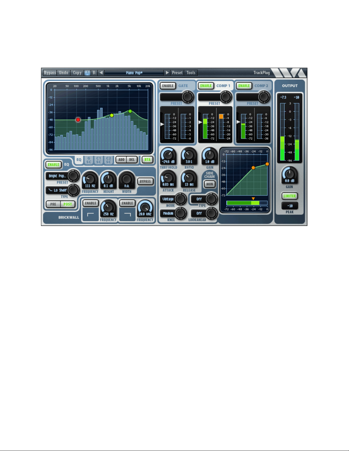
4.3 User Interface

The TrackPlug EQ interface is shown above. At the top is the frequency response display, which shows the frequency response of the current EQ. The frequency response display contains a number of control handles, drawn as colored balls, which correspond to EQ bands; clicking a handle will select that EQ band for editing, dragging a handle will change the parameters for the EQ. The band that is selected shows a halo around its control handle. The table below summarizes the operations that can be done inside the frequency response display:

EQ Section Control Mac

Adjust an EQ band's frequency and height

Adjust an EQ band's width Shift + click + drag

Add a new EQ band Double-click

Click + drag

Right click + drag

Shift + click + drag

Windows

Click + drag

-or-

Double-click

4. TrackPlug

Delete an EQ band Ctrl + click Show popup menu of all EQ bands listing all

parameters

Right-click on display

-or-

Shift-click on display

Ctrl + click

EQ Tabs

Just below the frequency response display are tabs for selecting which EQ is to be displayed and edited. Usually you will have the “EQ” tab selected, which means the main TrackPlug EQ. The other tabs are labeled “G-SC”, “C1-SC”, and “C2-SC” for Gate sidechain, Comp1 sidechain, and Comp2 sidechain, respectively. Click on these tabs when you want to edit one of the dynamics sidechain EQs. Note that the sidechain EQs are restricted to only a single band, and the EQ type must be lowpass, highpass, notch, or bandpass.

Add and Delete

The “Add” and “Delete” buttons are used to add and delete EQ bands. Clicking Add will create a new EQ band, and will display a new control handle. You can also add a band by double-clicking in the frequency response display. Up to 10 bands may be created. Clicking Delete deletes the current band. You can also delete a band by ctrl-clicking on its handle.

Enable

The Enable button enables/disables the entire EQ section. When disabled, the Enable button is not lit, and the EQ section is bypassed.

Bypass

The Bypass button bypasses the current band only. Toggling the bypass useful to hear the effect of a single EQ band. Any number of EQ bands can be bypassed. As you switch between different bands the bypass button will change to reflect the bypass state of the current band.

Pre and Post

The Pre and Post buttons control whether the EQ operates before the compressors (Pre button lit) or after the compressors (Post button lit). See the routing diagram at the start of this chapter for more information.

EQ Preset

The EQ preset selector button allow you to select factory or user presets for just the EQ section of TrackPlug. Clicking on the button will step to the next preset. Clicking on the preset name will display a popup menu of the current factory and user EQ presets.

Wave Arts Power Suite

EQ Type

The EQ Type selector button selects the EQ type of the current band. There are eleven different types, described in the “Equalization” section earlier in this chapter.

Frequency, Height, and Width knobs

These knobs let you set the frequency, height and width of the current band. If the selected EQ type does not support all three parameters, the unused parameters will display “n.a.” (not applicable). For the vintage and resonant shelf filters, the width knob serves as a resonance control by displaying values in units of “Q” rather than octaves.

Note that the EQ Type, Frequency, Height, Width, and Bypass controls will change as you select different bands to reflect the state of the currently selected band. Also note that the EQ preset affects neither the brickwall settings nor the sidechain EQ settings nor the EQ Enable button.

EQ display range

The vertical range of the EQ display can be changed by the user, allowing more subtle editing/viewing of the EQ response. Simply SHIFT-click (or right-click for PC users) on the vertical axis at the left of the EQ display to see a popup menu listing the ranges. The ranges are -24 to 24 dB, -12 to 12 dB, and -6 to 6 dB. TrackPlug will remember the last used setting. When using the zoomed-in ranges (+/- 12 and +/- 6 dB) it is possible that the EQ control handles will be off the display and will not be drawn. In this case you can select one of these bands by using the SHIFTclick popup menu, and then edit the values using the EQ parameter knobs.

Brickwall filter

The brickwall filter has an enable button and a knob for both the lowpass and highpass brickwall filter. When one of the bands is enabled, a corresponding brickwall control handle appears in the frequency response display. You can edit the brickwall frequency by dragging the control handle or dragging the knob.

Real Time Analyzer (RTA)

To enable the RTA, click on the RTA button below the EQ display (note that the RTA function is not enabled when running AAX DSP format). The RTA display appears overlaid on the EQ display. Further customization of the RTA modes is accomplished by SHIFT-clicking (or right-clicking for PC users) on the vertical dB axis at the left of the EQ display. This creates a popup menu showing the various RTA options below the options for selecting the EQ axis range. The RTA options include RTA range, RTA pre/post, and show/hide RTA axis.

4. TrackPlug

RTA range. Select the dB range you wish to view. The choices are -144 to 0 dB, -

96 to 0 dB, and -48 to 0 dB. Note that when the 48 dB range is selected, and the EQ is set to -24 to +24 dB, there is a one-to-one correspondence between the RTA levels and the EQ display. Hence if you move the EQ up by 6 dB you should see the same 6 dB rise in RTA levels, assuming the RTA is running post EQ.

RTA pre/post. Select “RTA Pre EQ” to run the RTA before the EQ, hence the RTA levels you see are before the EQ processing is applied. Select “RTA Post EQ” to run the RTA after the EQ processing is applied. Referring to the TrackPlug routing diagram, the EQ can run either before or after the compressors based on the EQ pre/post mode. Because the RTA can run either just before or just after the EQ, there are four possible insert points for the RTA. When the EQ display is set to one of the dynamics sidechains, the RTA runs either just before or just after the corresponding sidechain EQ. In this case, the Pre mode is useful for seeing what frequencies can be used to trigger the dynamics processors, for example, to visualize the frequency range of a vocal “ess” sounds before setting the sidechain EQ parameters.

Show/Hide RTA axis. Select “Show RTA Axis” to display the RTA vertical axis instead of the EQ axis. The RTA axis is drawn in blue to distinguish it from the white EQ axis. In this mode, when an EQ edit is made, the axis temporarily reverts to the EQ axis during the edit, then changes back to the RTA axis when the edit is complete. Select “Hide RTA Axis” to hide the RTA axis at al l times; only the EQ axis will be displayed.

Wave Arts Power Suite

Dynamics

TrackPlug’s dynamics user-interface section is shown above. At t he top are the three overview sections for the Gate, Comp1 and Comp2.

Dynamics interface overview section

Each overview section shows the enable button, the prese t con trol, input and gain meters, and a threshold slider control. The overview section serves as a tab control to select the section for detailed editing below. Click on the name of the section to select that section for editing. The selected section is shown with a light background. The controls below the overview sections are specific to the current selected section and will change based on the section that is currently selected. In the figure above, Comp1 is the current selected section. Note that all the controls in the overview sections are functional regardless of which section is enabled. So, for example, you can turn on and off Comp2, or change its threshold, while Comp1 is selected for editing.

The reason to have the overview sections is to make it easy to select some presets, set thresholds, and get work done without having to bother with the detailed parameters of each section. So for example, if you were processing a dialog track, you could select a noise gate preset for Gate, a de-esser preset for Comp1, and a vocal compression preset for Comp2. Then you enable the sections, set your

4. TrackPlug

thresholds, and you’re done. If something requires further tweaking, select the section tab and go below into the detailed param eters.

Enable

The Enable button enables/disables the corresponding dynamics section. When disabled, the Enable button is not lit, and the dynamics section is bypassed.

Preset

The preset selector button allow you to select factory or user presets for each dynamics section of TrackPlug. Clicking on the button will step to the next preset. Clicking on the preset name will display a popup menu of the current factory and user EQ presets.

Input and Gain meters

Each section meter shows an input meter on the left and a gain reduction meter on the right. The input meter shows the signal level coming into the dynamics section and the gain reduction meter shows the amount of gain reduction being applied. The input meter display depends on the dynamics mode and sidechain mode. If the dynamics mode is peak the meter shows peak values; if the mode is RMS the input meter shows RMS values. RMS values are typically 3 to 10 dB lower than peak values, depending on the material. If the sidechain is in use, then the input meter shows the signal level resulting from sidechain processing.

The meters show both the minimum and maximum values since the last meter redraw. The meter is drawn with a dark color up to the minimum value, and drawn with a lighter color from minimum to maximum value. These types of meters are a Wave Arts innovation. The “min/max” meters let you see at a glance how much a signal is modulating. If the signal level is constant the meter bar will be a solid dark color. If the signal level is modulating rapidly, this is shown by a large light section. The size of the light section indicates how much a signal is changing dynamically.

The vertical range of the dynamics attenuation meters can be selected by the user. Simply SHIFT-click (or right-click for PC users) on the axis to the right of the attenuation meter to see a popup menu list ing the ranges. The ranges are: -36 to 0 dB, -24 to 0 dB, -12 to 0 dB, and -6 to 0 dB. A different range can be selected for each dynamics meter. TrackPlug will remember the last used setting for each meter.

Threshold control

The input meter has a triangular control that lets you set the input threshold level. Drag the control up and down to change the threshold.

Wave Arts Power Suite

Dynamics response display

The detailed dynamics interface is highlighted by the dynamics response display on the right hand side. The dynamics response graph shows how input levels map to output levels. The default mapping, obtained with a ratio of 1:1, is shown as a straight diagonal line. A compressor with ratio greater than 1 will have a knee point above which the response bends to become more horizontal. The x-coordinate of the knee point is the threshold level. Hence, input values above the threshold will be attenuated. Similarly a gate with a ratio greater than 1 will have a knee point below which the response bends to become more vertical. In this case, input levels below the threshold are attenuated.

Below the dynamics response is a horizontal input meter. This shows the same information as the vertical input meter in the overview section.

The dynamics response contains several control handles that allow you to change the response directly. The controls differ for the gate and the two compressors. The table below describes how the handles can be used to change the parameters.

Compressor (Orange Handles) Control Mac or Windows

Adjust threshold and gain Click knee handle + drag Adjust threshold, gain and ratio so right

handle stays at same point Adjust ratio Click right handle + drag up/down

Adjust threshold

Shift-click (Mac) or right-click (Win) knee

handle + drag

Click orange triangle above input meter +

drag left/right

The compressor knee dragging is cleverly designed to let you adjust threshold, ratio and gain with a single mouse operation. Normally, dragging left-right changes the threshold and dragging up-down changes the gain. However, if you hold down the Shift key (or the right mouse button on Windows), the graph will pivot on the right handle, so dragging up-down will change the ratio as well.

Gate (Blue Handles) Control Mac or Windows

Adjust threshold and gain Click knee handle + drag Adjust threshold Adjust ratio Click bottom handle + drag left/right

Click blue triangle above input meter + drag

left/right

Detailed dynamics controls

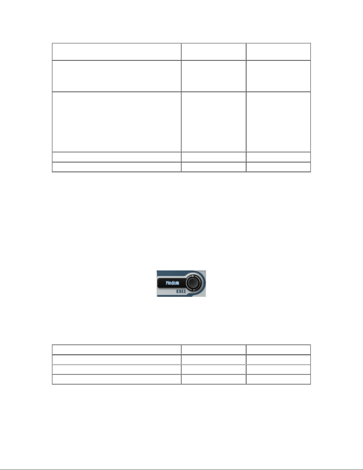
Knobs are provided for the Threshold, Ratio, Attack, Release, and Gain controls. In addition, there are selector controls to set the dynamics mode, knee curvature, and

4. TrackPlug

lookahead delay. These parameters are described elsewhere in this chapter. The sidechain is setup using two controls: a selector control for sidechain type and a monitor button. If the monitor button is lit, then the dynamics section outputs the sidechain signal. This will usually be the input signal processed through the sidechain EQ; however if the sidechain type is off, the monitor will simply pass the input signal, effectively bypassing the dynamics section. If an external sidechain source is selected, the monitor will pass the external source. This is a good way to verify the proper external source is being used.

Output section

TrackPlug's output section user-interface is shown below:

The stereo output meters have peak indicators above the meters. If the value exceeds 0 dB the display font turns red. Clicking on either indicator resets both channels to -96 dB. Right-clicking (Windows) or shift-clicking (Mac) on either value will automatically normalize the output gain to give a peak of -0.1 dB.

Below the meters is the output gain control, and below this is the peak limiter control. The peak limiter is enabled when the Limiter button is lit. When enabled, peaks that exceed -0.1 dB are automatically limited. The display below the limiter

Wave Arts Power Suite

shows the peak signal level before limiting; this will be displayed in red text if it is above 0 dB. Click on the display to reset it to -96 dB.

4.4 Parameters

This section lists all the internal parameters of TrackPlug and shows the range of values as would be displayed by a generic parameter-value plug-in interface. Most of these parameters have a one to one correspondence with controls on the user interface.

Each of TrackPlug’s 10 EQ bands has the following parameters:

Parameter name Values

Band Enable 0 = Off, 1 = Bypass, 2 = On Type 0 = Parameteric,1 = Low shelf, 2 =

High shelf, 3 = Vintage low shelf, 4 = Vintage high shelf, 5= Lowpass, 6 = Highpass, 7 = Bandpass, 8 = Notch, 9 = Resonant low shelf, 10 = Resonant high shelf

Frequency 20 – 20000 Hz Height -24db - +24db Width 0.01 - 5.0 octaves (or Q)

Each of TrackPlug’s three dynamics processors has the following parameters:

Parameter name Values

Dyn Enable 0 = Off, 1 = On Dyn Knee 0 = Soft, 1 = Medium, 2 = Hard Dyn Thresh Dyn Ratio 1 to 50 Dyn Gain -24 to +24 dB Dyn Attack 0.1 to 1000 msec Dyn Release 1 to 5000 msec Dyn Mode 0 = Clean peak, 1 = Clean RMS, 2 = Vintage

-96 to 0 dB

peak, 3 = Vintage RMS, 4 = Vintage Warm

AAX: 2 = Vintage peak, 3 = Vintage RMS, 4 = Vintage Warm

Dyn Lookahead 0 = Off, 1 = 1 msec, 2 = 2 msec, 3 = 5 msec Sidechain Mode 0 = Off, 1 = Internal EQ, 2 = Internal EQ

Compare, 3 = Internal EQ Invert, 4 = External EQ, 5 = External EQ Compare, 6 = External EQ Invert

Sidechain Monitor 0 = Off, 1 = On Sidechain EQ Type 5= Lowpass, 6 = Highpass, 7 = Bandpass, 8 =

Notch

4. TrackPlug

Sidechain EQ Freq 20 – 20000 Hz Sidechain EQ Width 0.01 - 5.0 octaves

The remaining TrackPlug parameters are listed below:

Parameter name Values

EQ Routing 0 = Pre, 1 = Post EQ Enable 0 = Off, 1 = On Brickwall Low Enable 0 = Off, 1 = On Brickwall Low Freq 20 – 20000 Hz Brickwall High Enable 0 = Off, 1 = On Brickwall High Freq 20 – 20000 Hz Output Gain -18 to +18 dB TrackPlug Enable 0 = Off, 1 = On Limiter Enable 0 = Off, 1 = On

4.5 Parameter Descriptions

EQ Parameters

The TrackPlug equalizer is described in detail in the section on Equalization earlier in this chapter.

Band Enable — This is an internal parameter that is controlled by the Add/Delete buttons and the Bypass button. Each EQ band is either deleted (that is, inactive and not displayed in the interface), enabled, or bypassed.

Type — Parametric, Low shelf, High shelf, Vintage low shelf, Vintage high shelf, Lowpass, Highpass, Bandpass, Notch, Resonant low shelf, Resonant high shelf.

Frequency — For parametric, notch, and bandpass filters, this is the center frequency; for shelf, lowpass, and highpass filters, this is the cutoff frequency. Range is 20-20,000Hz.

Height — Gain/attenuation for the currently selected EQ band (parameric and shelf filters only). Range is -24dB to +24dB.

Width — Bandwidth in octaves. The higher the number, the wider the filter, and vice versa. Applies only to parametric, bandpass, and notch filters. Range is 0.01 to

5.0 octaves. The vintage and resonant shelf filters use the width parameter to control resonance in units of “Q”; for the vintage shelf the range is 0.707 to 1.414, for the resonant shelf the range is 0.5 to 5.

Dynamics Parameters

Wave Arts Power Suite

The TrackPlug dynamics processor is described in detail in the section on Dynamics earlier in this chapter.

Dyn Enable — When off, the dynamics section is bypassed. Dyn Knee — Sets the dynamics knee shape; options are soft, medium and hard. Dyn Thresh — Level above which the compressor is active, or below which gate is

active. Range is -96dB to 0dB. Dyn Ratio — Controls how much gain reduction is applied as input level passes

threshold.

Dyn Gain — Dynamics makeup gain. Dyn Attack — Attack time in msec. Dyn Release — Release time in msec. Dyn Mode — Sets the dynamics mode. Options are: Clean peak, Clean RMS,

Vintage peak, Vintage RMS, Vintage Warm. AAX options are: Vintage peak, Vintage RMS, Vintage Warm.

Dyn Lookahead — Sets the lookahead time. Lookahead is useful when gating to provide a bit more time for the gate to restore gain prior to an onset.

Sidechain Mode — Set the sidechain source and mode. The sidechain modes are described in detail earlier in this chapter.

Sidechain Monitor — enables sidechain monitoring. Sidechain EQ Type — Sets the type of the sidechain EQ. Options are Lowpass,

Highpass, Bandpass, and Notch.

Sidechain EQ Freq — Sets the cutoff or center frequency of the sidechain EQ. Sidechain EQ Width — Sets the width of the sidechain EQ, applicable only when

bandpass and notch types are selected.

Global Parameters EQ Routing — Sets the position of the EQ module in TrackPlug's signal processing

chain. See the routing diagram at the start of this chapter for details. When routing is set to "Pre," the EQ is processed before the compressors. When set to "Post," the EQ is processed after the compressors.

EQ Enable — Enables or bypasses the EQ section.

4. TrackPlug

Brickwall Low Enable — Enables or bypasses the brickwall lowpass filter. Brickwall Low Freq — Sets the brickwall lowpass filter cutoff. Brickwall High Enable — Enables or bypasses the highpass brickwall filter. Brickwall High Freq — Sets the brickwall highpass filter cutoff. Output Gain — Sets the output gain. TrackPlug Enable — Enables or bypasses TrackPlug. This parameter is controlled

by the bypass button in the TrackPlug preset and menu bar. Limiter Enable — Enables or bypasses the peak limiter.

Wave Arts Power Suite

4.6 Specifications

Description Operating Systems Windows 7/8; Mac OS X 10.6 or higher

Plug-in Formats VST, AU, AAX, AAX DSP, RTAS, DirectX, MAS Sampling Rates up to 192 kHz I/O Formats mono-mono, mono-stereo, stereo-stereo

Channel strip with 10-band EQ, RTA, 2 compressors, gate, brickwall filter, and peak limiter.

4.7 Presets

TrackPlug global presets are listed below. The presets are descriptively named.

Category Preset name

General Default Drums Industrial Kick

Another Top Ten Kick Drum Punchy Kick Tight Bright Snare Good Ol' Snare Hit Snare Big Attack Snare Snare 1 Great Toms!! Beastly Drum Loop Beastly Drum Loop 2 Rock Drum Room 1 Rock Drum Room 2 Distorted Drum Loop Nook the Drum Room

Guitar Filter Gu itar Funk

From Pod to Metal God Acoustic Gtr Teeny Toy Guitar Ukelelephone

Bass Bass Channel

Walkin' Jazz Bass

Keyboard Piano Pop

Jazz Piano Ballad Horns Sax Solo Vocals Vocal Showstopper

Warm Rap Control

Angry Rapper

Songstress in my Ear

Sexy Pop Diva

Female R+B Ballad

4. TrackPlug

Effected Vox 1 Mix Very Nice 2-Mix Compress

Aggressive Rock 2-Mix

TrackPlug also ships with TrackPlug v4 presets, listed below:

Category Preset name

Drums Drums v4

Drums - Squisher v4 Drums - Squasher v4 Drums - Tighter v4 Kick v4 Snare 2 v4 Snare 3 v4 Toms v4 Hi-hats - Cymbals v4

Guitar Acou stic Guitar v4

Acoustic Gtr 2

Bass Bass v4

Bass - Acoustic v4 Bass - Attack v4

Bass - Attackier v4 Keyboard Piano v4 Horns Horns v4

Sax v4 Vocals Vocal - Female v4

Vocal - Male v4

Voiceover - Female v4

Voiceover - Male v4 Mix Mix - Dance v4

Mix - Rock v4

Master Plug v4

10 Band EQ v4

The Works v4 Special Xtreme Beat v4

Xtreme Vocals v4

What Dynamics? v4

Noise Filter v4

Telephone v4

Telephone - Screaming v4

EQ presets

Trackplug EQ presets are listed below.

Category Preset name

General 4-band Default

Brighter Warmth Biting Mid-range

Wave Arts Power Suite

Noise reduction Hum 60Hz

Drums Simple Kick Solution

Guitar Acoustic Gtr 1

Bass Modern Rock Bass

Vocals Male Vox 1

Fat-Bottomed Pipeline Xylophonated Comb the Area!! Telephone Transmission Old Time Radio Show

Hum 50Hz NTSC PAL-SECAM

Another Kick Drum Saved D112 Kick Industry Kick Snare 1 Old Snares Never Die Typical Snare Better Snare Classic Snare Snare De-ringer Alien Snare Drum Narrow Drum Band Tingly Sidestick Synthetic Sidestick Tom Control Vintage Toms Make Room for Tom When Toms Ruled the Earth Punchy Tom Cymbal Sizzle Subtle Cymbal Shine Jazzy Ride Cymbal Ride Cymbal Recipe Hi Hats

Acoustic Gtr 2 Nu-Metal Guitar Typical Death Metal Filtered Funk Guitar Ukelelephone

Gave my Bass Wood Deep Bass Bass DI Helper Snappy Upright BAss

Female Pop Vox Airy Back Vox Big Ballad Vox Stimulated BVox

4. TrackPlug

Keyboard Bright Pop Piano

Warm Piano Strings Disco String Section Horns Smoky Jazz Sax

Sax with Attitude

Gate presets

Trackplug Gate presets are listed below.

Category Preset name

General Default

Typical Fast Gate

Drums Tight Kick

Looser Kick Snare 1 Snare 2 Tom Quick Decay Tom Long Decay Lo Tom Long Decay Room Mic-triggered by Snare

Compressor presets

Trackplug Compressor presets are listed below.

Category Preset name

General Default

Transparent Gentle Compress Gentler Attack Brings Out Attacks

Drums Kick Tightener

Much Roomier Kick Snare After-Ring Snappy Snare Softer Snare Attack Thunderous Tom Drum Room Mics

Guitar A Gtr 1

Funk Guitar Hard Attack Slight Crunch Rhythm Guitar Harsh Guitar Tamer

Bass Bass Evener

Bass Add Punch Mid-Range Bass Attack Forgot to change Bass Strings Clacky Bass

Wave Arts Power Suite

Percussive Upright Bass

Vocals Out Front vocals

Classic Warm Vocal Subtle Vocal Control Female Pop Vox Angry Rock Vocal Punishes Pesky Plosives De-esser 1 De-esser 2

Keyboard 80's Pop Piano

5. MasterVerb

5.1 Overview

MasterVerb is a classic digital reverb with a spacious natural sound and a silkysmooth decay. Featuring multiple reverb algorithms, with comprehensive early reflection, equalization, and envelope control, MasterVerb is capable of reproducing a vast palette of reverberation effects. MasterVerb features the following:

 Choose between hall and plate late reverb algorithms.  Comprehensive early reflection selections, including halls, rooms, chambers,

plates, or special effect reflections.

 Independent room size and decay time parameters allow simulation of a

variety of spaces from bathrooms to cathedrals.

 Three band early and late equalizers allow detailed tone shaping.  Envelope generator for creating gate and reverse effects.  Character control lets you find the room sound you want in just seconds.

Wave Arts Power Suite

 Time response display shows relative levels of direct sound, early reflections,

and late reverb.

 Frequency response display shows the reverb decay in three dimensions.  Extremely CPU efficient algorithms

A diagram of MasterVerb’s audio routing and meter placement is shown below.

Env

Meter

Output

Meter

Wet

Delay

Dry

Delay

Early EQ Reflections

Late

Reverb

MasterVerb audio routing diagram.

Early

Envelope

Late

Wet

Dry

Output

Out

The input signal is split into wet and dry paths. The wet path is delayed by the wet delay (also known as pre-delay) and is then processed by the early damping equalizer. The wet signal is then split into early and late paths; the early path is processed with the early reflection generator, while the late path is processed by the late reverb. Note that the late damping equalizer is embedded in the late reverb algorithm. The early and late reverb components are mixed and fed into the envelope processor. The envelope processor is triggered by the non-delayed dry input signal, although this path is not shown in the diagram. The final wet signal is mixed with the delayed dry signal and the result is processed by the fina l output gain.

5.2 About MasterVerb

About Reverberation

When an object in a room produces a sound, a soundwave expands outward from the source reaching walls and other objects where sound energy is both absorbed and reflected. Assuming a direct path exists between the source and the listener, the listener will first hear the direct sound, followed by reflections off nearby surfaces, called early reflections. After a few tenths of a second, the number of reflected waves becomes very large, and the resulting reverberation is characterized by a dense collection of soundwaves traveling in all directions, called diffuse reverberation.

5. MasterVerb

The time required for the reverberation to decay 60 dB below the initial level is defined as the reverberation time. Generally, reverberation in a small room decays much faster than reverberation in a large room, because in a small room the soundwaves collide with walls much more frequently, and thus are absorbed more quickly, than in a large room.

Reverberation is a really important acoustic phenomenon. There is at most one direct path from the source to the listener, whereas there may be millions of indirect paths, particularly in a room where a sound can bounce around hundreds of times before being absorbed. Thus, in typical listening situations, most of the energy we hear from a sound source is actually reverberation.

The perception of reverberation depends on the type of reverberation and the type of sound. In small room with fast decaying reverberation, the reverberation imparts a tonal quality to the sound that is readily identified as a small room signature. In a larger room, the reverberation can create a background ambience that is easily distinguished from the foreground sound, and this is readily identified as a characteristic of large spaces. In this manner, reverberation imparts useful spatial information about the size of the surrounding space.

Early reflections arriving within the first 80 msec after the direct sound tend to become perceptually fused with the direct sound. Hence the early reflections modify the character of the sound itself whereas much later reverberation becomes associated with the background ambience. A prominent reflection that occurs soon after the direct sound will create a comb filtering effect, as frequencies are either amplified or attenuated due to the reinforcement or cancellation caused by adding the delayed reflection to the direct sound. This comb filtering effect happens with any reflection, but is most noticeable with very early reflections which cause broad frequency effects. The result is a timbre modification of the sound, possibly hollow sounding, which can readily be associated with an enclosed space or a small room.

Early reflections can also modify the apparent size of the sound source. Reflections that arrive in staggered order from the left and right directions confuse our sound localization perception. Instead of perceiving a narrowly localized sound source, the result will be a fuzzier, wider perception. Hence the early reflection pattern can affect both the timbre and apparent size of the source.

Reverberation that contains a lot of high frequency energy in the decay is associated with rooms that have hard, reflective walls, which do not readily absorb high frequencies. Similarly, reverberation that is dull sounding is associated with rooms that contain soft materials, such as plush carpets and drapes, which readily absorb high frequencies. In this manner, reverberation imparts useful information about the composition of the surrounding space.

Reverberation is also important for establishing distance cues. In a reverberant space, when the distance between the source and the listener is increased, the level of the direct sound decreases considerably, but the level of reverberation does not decrease much. Thus, the level of direct to reverberant sound can be used as a

Wave Arts Power Suite

distance cue, with dry (non-reverberant) sounds perceived as being close, and reverberant sounds perceived as being distant.

Reverberation gives information about the size and character of the surrounding space and the distance of the sound source. For recordings that are made with close microphone techniques, artificial reverberation must be added to restore spatial context. Reverb is thus an essential tool for imparting a sense of space to your recordings.

Reverb algorithms

Before digital reverbs were available, recording studios had to use other means to generate reverberation. One method required building a very reverberant room into which speakers and microphones were placed. Sounds to be reverberated were piped into the room, and the resulting reverb was picked up by the microphones. These rooms were known as reverb chambers.

An alternative method of generating artificial reverb that requires much less space than a chamber is the plate reverb. Essentially the reverb chamber is replaced by a suspended steel plate. Signals are injected into the plate using transducers mounted on the plate, causing the plate to vibrate. The resulting vibrations are picked up by additional transducers mounted on the plate. The reverberation created by a plate is quite dense and diffuse. Although a plate’s reverberation doesn’t sound like a room’s reverberation, the sound is pleasing and often used on vocals and drums.

Digital reverbs model acoustical and mechanical reverbs using a large number of delay lines through which the signal is recirculated. Each reverb algorithm has its own characteristic sound and idiosyncrasies. MasterVerb contains two reverb algorithms, the Hall and Plate algorithms. The Hall algorithm, inherited from MasterVerb v4, sounds like a concert hall. The Plate algorithm sounds like a plate reverb, characterized by a very rapid buildup of densely spaced reflections.

The Hall algorithm can be scaled to sound like small rooms or very large spaces. Scaling a reverb algorithm is done by scaling the delays within the algorithm. The Plate algorithm can also be scaled but because the Plate response is so dense, the effect of scaling the Plate is less pronounced than scaling the Hall.

Early reflections

MasterVerb models the early reflection pattern using a stereo tapped delay line. Each individual reflection is implemented with a single tap in the delay line. Typical reflection patterns may have 25 to 60 reflections per channel. The output of the tapped delay line is further processed by a diffuser circuit that smears out the response in time, causing the reflections to sound less discrete.

The reflection patterns in MasterVerb are based on real and synthetic reverberation responses. Patterns are included for real acoustic spaces including halls, a

5. MasterVerb

cathedral, and some rooms, and for synthetic reverb responses including chambers and plates. The Anechoic reflection type has a single unit gain reflection at time 0 (in both left and right channels), so it simply passes the input signal unchanged to the diffuser circuit.

The user should note that the CPU processing required for the early r eflection generator is about the same as for the late reverb algorithm, hence if you need a really CPU efficient reverb, try bypassing the early reflection generator by selecting the “Anechoic” pattern, then set the late/early mix to 100% late.

Envelope

MasterVerb’s envelope control is used to alter the amplitude response of the reverb. When the envelope control is enabled, the output of the reverberator is amplitude modulated by the envelope. The envelope itself has three segments, attack, hold, and release, and is triggered when the input signal exceeds the threshold. This is shown in the diagram below. The envelope is nominally at gain 0. When the input signal exceeds the threshold, the envelope is triggered. This causes the envelope to increase to unit gain with rate specified by the attack time parameter. The envelope then holds for the hold time, and finally releases according to the release time parameter. The envelope will retrigger (return to attack state) whenever the input exceeds the threshold.

threshold

envelope

attack hold release

Diagram of envelope triggered by input sound.

The envelope makes it easy to set up gated reverb effects, where the wet reverb is turned on when there is an input, and then abruptly shuts off after a certain amount of time.

Wave Arts Power Suite

Advanced users may want to know that the attack and release envelope segments are generated using exponential shapes. Hence the attack and release segment times are actually exponential time constants. For attack segments, the segment will have grown to 63% of full scale (-4 dB) after the attack time. It will continue to grow to 0 dB during the hold segment. Release segments will decay -8.7 dB every release time. The exponential shapes sound very natural. Use your ears to adjust the time constants to suit.

Mixing with MasterVerb

For music production, it is common to place a reverb plug-in on an aux bus in your host application program, and use the aux send on the tracks you want to be processed with reverb. In this case the reverb wet/dry mix should be set to 100%, therefore the aux return gain will set the wet level, and the track gain will set the dry level. Using reverb in this way not only saves CPU resources but lends to a more natural sound, since each track is in a sense sharing the same “space”.

When using reverb as an insert effect, you will want to use much drier mix levels to prevent the sound from becoming too muddy with reverb. The presets are designed assuming the reverb will be used as an insert effect, so the preset mix levels are a good place to start.

Beginning users of MasterVerb may be confused by the Wet/Dry and Late/Early controls. The Wet/Dry mix sets the wet mix level – 100% is all wet, 0% is all dry. Similarly the Late/Early mix sets the late mix level – 100% is all late, and 0% is all early. Hence the controls give you the most wet effect when pushed to the maximum 100% value. The confusion arises from the placement of the labels on the UI – moving the knob to 0% points the knob indicator to the Wet (or Late) label, and moving the knob to 100% points the knob indicator to the Dry (or Early) label, which is counter to the meaning. Think of the controls as simply “Late” and “Wet” controls, and remember that larger parameter values produce a wetter sound.

5.3 User Interface

In addition to the standard controls and displays found in other Wave Arts plug-ins, MasterVerb contains several custom displays which facilitate operation and allow you to visualize the inner workings of the plug-in. The displays are grouped together in the upper left of the MasterVerb window. They include the character control, the early and late damping controls, the time response display, and the frequency response display.

5. MasterVerb

Character control

The character control allows you to simultaneously adjust the reverb time and the room size by clicking on the red ball and dragging it within the control area. Moving the control left-right changes both the early reflection size and the late reverb size. Moving the control up-down changes the reverberation decay time. Small sounding spaces are selected at the lower left, large spaces at the upper right.

Damping controls

Each of the damping controls shows the frequency response of the three band shelving filter that implements the damping. For the early damping control the vertical axis is labeled in dB, while the late damping control vertical axis is labeled in terms of reverb time scale factor. The colored control handles allow the adjustment of the band levels and frequency crossover points. The midrange band controls (light blue) are fixed at 640 Hz and can only be moved up and down to adjust the level.

The user should note that the early damping control affects all the reverberation, both early reflections and late reverb. It is called “early” to distinguish it from the late damping that only affects the response of the late reverb decay.

Wave Arts Power Suite

Time response display

The time response displays shows a caricature of the actual time response of the reverb. The direct response is shown as a vertical white bar (in the above diagram it is on the far left at time 0). The early reflection response is shown as a series of green vertical lines that represent the individual reflections. The late reverb response is shown as a green shaded region. The time scale of the display can be changed by clicking on the x1 and x10 controls at the upper right; this changes the maximum display time from 250 msec to 2.5 seconds.

When the envelope is enabled, the envelope response is shown in the time display as a blue shaded region. This allows the user to visualize the attack, hold, and release times.

Frequency response display

The reverb frequency decay plot is a three-dimensional plot that shows the frequency response of MasterVerb during the reverb decay. The plot allows easy visualization of both the overall equalization due to the early damping control and the time dependent equalization due to the late damping control. The vertical axis represents amplitude in dB, the axis that runs from left to right represents time in seconds, and the rear axis represents frequency in Hz. Note that low frequencies are shown on the right in green; high frequencies are shown on the left in blue.

5. MasterVerb

From a frequency standpoint, this plot is a mirror image of the damping controls which have the frequency plotted left to right as is typical.

The frequency response is principally affected by the Reverb Decay Time, Early Damping, and Late Damping parameters. Changing the decay time causes the entire surface to pivot about time 0 as the decay slopes at all frequencies are changed. Changing the early damping affects the initial equalization (the frequency response at time 0). Changing the late damping affects the decay slope. The characteristic plot always shows the 100% wet response, assuming wet delay is 0, and is not affected by the Wet/Dry, Wet Delay or Output parameters.

5.4 Parameters

This section describes all the internal parameters of MasterVerb as would be displayed by a generic parameter-value plug-in interface. Most of these have a one to one correspondence with controls on the user interface.

Parameter name Values

Enable 0 = Off, 1 = On Reflection Type 0 = Bypass, 1 = Hall1, 2 =

Hall2, 3 = Cathedral, 4 = Room1, 5 = Room2, 6 = Chamber1, 7 = Chamber2, 8 = Plate1, 9 = Plate2, 10 = Echo,

11 = Ping-pong Reflection Size x0.5 to x1.5 Early Damping Lo Freq 20 to 640 Hz Early Damping Lo Gain -24 to 0 dB Early Damping Mid Gain -24 to 0 dB Early Damping Hi Freq 640 to 20,000 Hz Early Damping Hi Gain -24 to 0 dB Late Reverb Type 0 = Hall, 1 = Plate Late Reverb Decay Time 0.5 to 60 sec Late Reverb Size x0.5 to x1.5 Late Damping Lo Freq 20 to 640 Hz Late Damping Lo Scale x0.25 to x4 Late Damping Mid Scale x0.25 to x4 Late Damping Hi Freq 640 to 20,000 Hz Late Damping Hi Scale x0.25 to x4 Envelope Enable 0 = Off, 1 = On Envelope Thresh -36 to 0 dB Envelope Attack Time 1 to 2000 msec Envelope Hold Time 1 to 2000 msec Envelope Release Time 1 to 2000 msec Dry Delay 0 to 500 msec Wet Delay 0 to 500 msec

Wave Arts Power Suite

Wet/Dry Mix 0 to 100% Late/Early Mix 0 to 100% Output Gain -18 to 18 dB Diffusion 0 to 100%

5.5 Parameter Descriptions

Following is an explanation of MasterVerb's parameters: Enable — Turns MasterVerb on and off. This internal parameter is controlled by the

Bypass button in the MasterVerb menu bar. When the Bypass button is lit, the internal enable is off, and vice-versa.

Reflection Type – Sets the early reflection pattern. The early reflection pattern consists of a set of discrete echoes, typically spanning no more than two hundred milliseconds. A number of reflection patterns are provided, including halls, rooms, chambers, and plates. The halls and rooms are reflection patterns derived from actual acoustical spaces. The chambers and plates are dense collections of reflections derived from synthetic responses. The Anechoic type is a single unit gain echo at time 0, which passes the input signal unchanged, althoughit is still processed by the diffuser. Other special effect echo types are included.

Reflection Size – Scales the size of the early reflection pattern, ranging from x0.5 (50%) to x1.5 (150%). Smaller sizes will sound like a smaller space, and larger sizes will sound like a larger space.

Early Damping Parameters

The early damping EQ affects all signals going into the wet path of the reverb, therefore it is used to change the equalization of both the early reflections and the late reverb. It could also be called “Wet Equalization”. Typically the EQ is set up to attenuate high frequencies, because reverberation is usually not very bright due to the absorption of high frequencies by materials in the room. The damping EQ is a three band shelf equalizer with lo, mid, and high gains, and adjustable band edge frequencies.

Early Damping Lo Freq – Sets the transition frequency between the low band and mid band of the early damping EQ.

Early Damping Lo Gain – Sets the gain in dB of the low band of the early damping EQ.

Early Damping Mid Gain – Sets the gain in dB of the mid band of the early damping EQ.

5. MasterVerb

Early Damping Hi Freq – Sets the transition frequency between the mid band and

high band of the early damping EQ. Early Damping Hi Gain – Sets the gain in dB of the high band of the early

damping EQ. Late Reverb Type – Selects the late reverb algorithm. There are currently two

completely independent reverberation algorithms, the Hall algorithm and the Plate algorithm. The hall algorithm sounds like a concert hall, which can be scaled to sound like small rooms or very large spaces. The plate algorithm sounds like a plate reverberator. An actual plate reverb is created by attaching transducers to a large steel plate suspended from wires; the transducers send the dry sound into the plate, which vibrates, and the resulting reverb is picked up by other transducers. Plate reverbs have extremely dense and diffuse reverberation.

Reverb Time — Sets the decay time of the late reverberation in seconds, from 0.5 sec to 60 sec. The reverberation time is the time it takes for frequencies near 500 Hz to decay by 60 dB. For typical input sounds, the reverberation will be essentially inaudible after decaying 60 dB, so the Reverb Time specifies the effective length of the reverberation tail in seconds. The Reverb Time parameter is independent of the Reverb Size parameter.

Reverb Size — Scales the size of all delays within the late reverberation algorithm, ranging from x0.5 (50%) to x1.5 (150%). A Reverb Size of x0.5 sounds like a very small space, such as a bathroom or closet, x1.0 sounds like a concert hall, and x1.5 sounds like a very large room, such as an aircraft hangar or stadium. The Reverb Size parameter is independent of the Reverb Time. In general, small rooms sound best with short decay times, and large rooms sound best with longer decay times.

Late Damping Parameters

The late damping EQ is a three band shelf equalizer that is embedded in the late reverb algorithm. The late damping EQ affects the sound that is recirculating in the late reverb algorithm. Hence, if the late EQ is set to attenuate high frequencies, this means the high frequencies will decay faster than the low frequencies. Thus, the late damping EQ sets the frequency dependent decay time of the reverb. The equalization gains are specified as reverberation time scaling factors relative to the nominal reverb time, i.e. the Reverb Time parameter which is defined at 500 Hz. For example, a scaling of x2 means the reverberation will be twice as long as the Reverb Time parameter, while a scaling of x0.5 means the reverberation will be half as long. The late damping EQ is a three band shelf equalizer with lo, mid, and high gains, and adjustable band edge frequencies.

Late Damping Lo Freq – Sets the transition frequency between the low band and mid band of the late damping EQ.

Late Damping Lo Scale – Sets the reverb time scaling of the low band of the late damping EQ.

Wave Arts Power Suite

Late Damping Mid Gain – Sets the reverb time scaling of the mid band of the late

damping EQ. Late Damping Hi Freq – Sets the transition frequency between the mid band and

high band of the late damping EQ. Late Damping Hi Scale – Sets the reverb time scaling of the high band of the late

damping EQ. Envelope Enable – Enables or disables the envelope. When the envelope is

enabled, the wet reverb sound is modulated by the envelope. When the envelope is disabled, it is bypassed.

Envelope Threshold – Set the trigger threshold of the envelope, from -36 to 0 dB. Envelope Attack Time – Sets the attack time of the envelope, from 1 to 2000

msec.

Envelope Hold Time – Sets the hold time of the envelope, from 1 to 2000 msec. Envelope Release Time – Sets the release time of the envelope, from 1 to 2000

msec. Dry Delay — Sets the delay of the dry signal, ranging from 0 to 500 milliseconds.

By delaying the dry signal, the wet reverberation can precede the dry signal. One use of this parameter is to create a simulated reverse reverb effect, where the reverb builds up and then ends with the dry sound.

Wet Delay — Sets the delay of the wet output, ranging from 0 to 500 milliseconds. Wet Delay is often called “Pre-Delay”. Wet Delay is used to achieve an additional echo effect in the reverberation by delaying the reverberation relative to the dry sound. Wet Delays larger than 100 msec can be used to simulate large spaces such as stadiums and canyons. The Wet Delay will be inaudible unless the Wet/Dry Mix is set to something greater than 0%, so that both the wet and dry outputs are audible.

Wet/Dry Mix — Sets the amount of wet (processed) sound and dry (unprocessed) sound that is mixed together to create the output. 100% is all wet, 0% is all dry, and 50% is an equal mix of wet and dry sound. Effectively, the Wet/Dry parameter sets the perceived distance of the input sound: 100% sounds very distant, and 0% sounds very near.

Late/Early Mix – Sets the amount of late and early reverberation that is mixed together to create the wet reverb signal. The late reverberation comes from the late reverb algorithm. The early reverberation comes from the early reflection generator. The Late/Early Mix is used to set the definition of the early portion of the reverb response by mixing in early reflection with the late reverb. Note that if the

5. MasterVerb

early reflection type is set to Bypass, then the early signal is the dry signal. Typically, if the early reflection type is set to Bypass, you will want to set the Late/Early mix to 100% (all late) and then use the Wet/Dry mix to mix in dry signal.

Diffusion — Sets the extent to which individual echoes propagating in the reverb are spread in time. Low values of diffusion produce reverberation that will have audibly discrete early echoes, almost granular sounding, whereas high values of diffusion tend to produce a softer, fuzzier sounding response. The Diffusion parameter affects the diffusion of both the early reflections and the late reverberation algorithm.

Output Gain — Sets the overall output gain in decibels. This gain is applied to the output of the wet/dry mix, therefore the gain does not affect the relative levels of wet and dry sound.

5.6 Specifications

Description Operating Systems Windows 7/8; Mac OS X 10.6 or higher

Plug-in Formats VST, AU, AAX, RTAS, DirectX, MAS Sampling Rates up to 192 kHz I/O Formats mono-mono, mono-stereo, stereo-stereo

Multi-algorithm reverberator with hall and plate algorithms, comprehensive early reflection patterns, and envelope control.

5.7 Presets

Preset Name

Default Warm Booth Bright Slapback Vocal Doubler Room Lead Vocal Room Small Bright Room Brassy Bright Room Huge Padded Room Chamber Bright Guitar Chamber Big Drum Chamber Vocal Stage Choir Loft Space for Metal Guitar Small Dark Church Concert Hall

Wave Arts Power Suite

Small Hall Bloom Hall Opera Hall Drum plate Tame Plate Vocal Plate 80's Big Hair Snare Tight Gated Toms Shotgun Snare Gated plate Reverse Plate In the Cave Ghostly Ending Gigantic Trailing into the Mist Pad Generation Echo-verb Trippy Echoes Vox Splatter-Delay Filtered SlapDelay

MasterVerb also ships with MasterVerb v4 preset, listed below:

Tiny Room, Bright v4 Tiny Room, Muffled v4 Studio v4 Studio, bright v4 Studio, warm v4 Nightclub v4 Nightclub, bright v4 Nightclub, warm v4 Concert hall v4 Concert hall, bright v4 Concert hall, warm v4 Cathedral v4 Cathedral, bright v4 Outdoor ambience v4 Small resonant space v4 PA System v4 Scatter Verb v4 Thud Verb v4 Menace Verb v4 Large Concert v4 Live Hall v4 Grand Hall v4 Gymnasium v4 Small room v4 Bathroom v4 Oil Drum v4 Delay Verb v4 Dark Room v4

5. MasterVerb

Church v4 Medium Room v4 Richochet v4 Slapback Echo v4

6. FinalPlug

6.1 Overview

FinalPlug is a lookahead peak limiter with bit depth truncation and noise shaped dithering. Here are some of FinalPlug’s key features:

 Sonically transparent peak limiting, for use as peak limiter or volume

maximizer.

 Auto-release mode  Bit depth truncation from 4 to 24 bits.  TPDF dithering.  Comprehensive noise shaping options.  Operation up to 192 kHz sampling rate.  Mono to mono or stereo to stereo operation.  Presets for CD and DVD-audio mast ering and track compression.

A diagram of FinalPlug’s audio routing and meter placement is shown below.

Wave Arts Power Suite

FinalPlug is most commonly used as the final plug-in to process a mix on the master output. It allows you to maximize the volume of a mix while preventing the sound from exceeding a certain level, so that digital clipping doesn’t occur. It is more flexible than normalizing, since you aren’t simply increasing the volume of the entire track by a constant gain. FinalPlug dynamically reduces peaks to be more in line with the rest of the signal, and with careful use, you can increase the perceived loudness of a mix by 6 to 12 dB without any audible artifacts.

If you are preparing a CD master, FinalPlug’s truncation and dithering features can be used to reduce the bit depth of your recording to 16 bits while minimizing the amount of quantization noise that can be perceived.

FinalPlug Limit

For AAX DSP, the FinalPlug Limit configuration runs just the peak limiter with no dither section. This is because the dither section is computationally expensive, so you can get more instances of just the peak limiter.

6.2 About FinalPlug

Peak Limiting

FinalPlug’s peak limiter can be used to do tasks ranging from light peak limiting to volume maximization to very heavy compression. The FinalPlug limiter detects peaks in the signal and very quickly reduces the input gain prior to the peak, preventing clipping. After the peak has passed, FinalPlug restores the input gain to the nominal level.

The peak limiter will limit any peak that exceeds the threshold level set by the user. The peak limiter uses a built-in lookahead delay to respond to peaks just before they occur. Both the lookahead delay and attack time are fixed at 1.5 milliseconds. This is designed according to the pre-masking phenomenon of the human auditory system whereby loud sounds effectively mask sounds that occurred just prior. Hence, any distortion caused by the rapid gain ducking will be effectively masked by the onset of the peak. The shape of the peak itself is unaffected by the gain ducking; this is in contrast to peak limiters that use wave shaping techniques. After the peak has passed, the gain is restored to nominal level according to the release time set by the user.

The release time is an important parameter. Short release times cause the gain to be increased rapidly after peaks. This is important when you want to aggressively compress a signal. However, short release times also cause the gain to modulate more deeply during steady audio signals, causing distortion. This is because with aggressive settings the peak limiter will be compressing each oscillation of the input signal; ducking the gain to allow the peak oscillation to pass, then quickly restoring the gain as the signal passes through 0.

6. FinalPlug

In contrast, long release times prevent distortion during steady audio signals. This is because the gain will be ducked on the onset of the signal and will stay ducked because the release happens so slowly. Hence the amount of gain modulation with each oscillation of the input is very small, and hence the distortion is greatly reduced compared to using a fast release time. However, the disadvantage of using a long release time is that it takes a long time for the gain to increase after loud sounds in the input. This can cause an audible pumping of the background level of the audio; each peak in the audio causes the background to be reduced in volume and then the background level increases slowly until the next peak. Furthermore long release times do not permit aggressive compression.

FinalPlug features an auto-release mode which dynamically chooses the optimum release time based upon t he program content. FinalPlug chooses the release time based on the crest factor of the input signal. The crest factor is an indicator of the peakiness of a signal; it is obtained by comparing the peak level of a signal to the average level. FinalPlug uses a short release time for input signals that are peaky, and it uses a long release time for signals that are steady. The implementation of the auto-release mode is a balance between low distortion operation, aggressive compression, and reduced pumping effects. The auto-release mode in FinalPlug achieves a nice balance, preventing distortion during steady tones even when compressing heavily, while reducing pumping effects and using fast release times when possible.

Lookahead peak limiters like FinalPlug are often used to increase the volume of a mix. In today’s “loudness wars”, this technique is often used to excess, creating ultra-compressed audio that can be quite fatiguing to listen to. One need only look at the digital content of a typical pop CD to see how hyper-compressed today’s music is. Readers are encouraged to read the following: “Current Trends in Mastering: The Loudness War”, by Mark Donahue, June 2003 Performer Magazine, and “What happens to my recording when it’s played on the radio?” By Frank Foti, Omnia Audio & Robert Orban, CRL/Orban.

Truncation and Dithering

FinalPlug also features bit depth truncation with dithering and noise shaping. Bit depth truncation typically occurs as the final step in mastering when the sample resolution must be reduced to fit on the recording medium. For example, compact discs (CDs) are recorded with 16-bit samples, whereas digital audio editors typically use 32-bit floating point sample format containing at least 24-bit sample resolution. Hence, the 24-bit resolution samples must be reduced to 16-bit prior to burning the CD. This is done by discarding the least significant bits, which is the definition of bit depth truncation.

Truncation wil l cause the addition of "quantization noise" and "quantization distortion" to the resulting signal. For low level signals, i.e. signals that are only a few bits in amplitude, the quantization distortion can sound very objecti onable. Dithering is a technique used to eliminate quantization distortion by adding a small amount of random noise to the signal prior to truncation. The added noise "dithers"

Wave Arts Power Suite

the signal between the various quantized output levels in such a way that the quantization distortion is converted to pure broadband noise. Hence, dithering adds noise to the signal in order to convert the objectionable quantization distortion to less objectionable noise. Dithering is thus converting distortion to hiss. FinalPlu g uses TPDF (triangular probability distribution function) noise for dithering. Mathematically, this is known to be the optimal type of noise to convert quantization distortion to noise that is uncorrelated with the original signal.

Noise shaping is a technique used to shape the spectrum of the quantization noise in order to make it less perceptible to the human ear. Typically, noise shapers push the quantization noise to higher frequencies to which the ear is less sensitive. However, there are many variations of noise shaping techniques in use. The user must decide which shape is best for the task at hand. In this spirit, FinalPlug provides a wide variety of noise shapes to choose from. Some of the shapes are similar to other noise shapers in common use.

It should be noted that dithering and noise shaping may offer fewer practical benefits than the marketing from many manufacturers would have you believe. This is because acoustic recordings typically contain much higher levels of noise than required to properly dither a signal. Hence, adding dithering will have no effect except to slightly increase the existing noise level. A study by D. W. Fostle (Audio Magazine, March, 1996) showed that very few recorded CDs have low enough noise floors to benefit from proper dithering and noise shaping. The advantages of dithering are even more tenuous when considering 24-bit media, like DVD-audio. Dithering and noise shaping will have benefits only when the original material has a noise floor below the quantization level of the final medium. This is unlikely when dealing with acoustically recorded material. However, purely synthetic material (more common these days) may indeed have very low noise floors and may benefit from proper dithering and noise shaping.

As shown in the above schematic, truncation and dithering occurs after peak limiting. Hence, the output level as shown by the output meters may slightly exceed the limiter ceiling level when dithering is active. This is because the dithering and noise shaping occurs after peak limiting. The effect is negligible for typical settings. We recommend that a ceiling of -0.1 dB be used for CD and DVDaudio mastering to allow a tiny bit of headroom for dither noise. Additional headroom may be needed when dithering signals at small bit depths, such as 8 bits.

6.3 User Interface

FinalPlug comes with a number of presets for both track compression and for final processing prior to CD or DVD-audio burning. If you want to dig deeper than the presets read the following sections on how to use FinalPlug.

The user interface for FinalPlug is shown at the start of this chapter. FinalPlug is separated into a peak limiter section on the left and a truncate/dither section on the right; each section has its own enable button at the top left. If you are using

6. FinalPlug

FinalPlug as a track compressor, just enable the limiter section and leave the truncation section disabled. Truncation should only be enabled if you are using FinalPlug as the last step prior to burning a CD or DVD. The one exception to this is if you are using the truncation section specifically to obtain bit truncation distortion effects.

Using the Limiter section

The peak limiter section has only three controls: threshold, ceiling, and release time. The output ceiling defines the maximum level the limiter will output. The threshold defines the input level at which limiting takes place. The easiest way to use the limiter is to first set the ceiling control to the desired peak output level, then lower the threshold to achieve the desired amount of compression. Adjust the ceiling and threshold by clicking on the triangular indicators next to the meters and dragging them up and down. If you continue to lower the threshold you will get increasingly more signal compression. At any time you can compare the limited signal with the unlimited signal by toggling the limiter enable control or the FinalPlug bypass control. Note that FinalPlug applies a constant gain equal to the different between the ceiling and threshold controls, so that even if limiting is not taking place, FinalPlug is applying a constant gain to the signal.

Three meters show the stereo input levels, stereo output levels and amount of limiter attenuation. At the top of the meters are peak indicators that show the maximum value achieved. Click on the indicators to reset them.

When the input exceeds the threshold, and limiting takes place, the attenuation meter simply shows the difference between the input and the threshold. Like other Wave Arts compression meters, the attenuation meter has a two color scheme to show the minimum and maximum attenuations: the dark red color extends from 0 to the minimum attenuation, while the bright red extends from the minimum to the maximum attenuation. Thus, the bright red section shows how much the attenuation is changing. If the attenuation meter is solid dark red, then this indicated the attenuation is constant. A large bright section indicates that the gain is rapidly changing across a large range, which would be the case for aggressive compression using a fast release time.

We recommend you enable the auto-release option, which causes FinalPlug to dynamically choose the optimal release time based upon the program content. If the auto-release option is disabled, you can manually select a release time from 1 msec to 1 sec using the slider.

Using the Truncate/Dither section

The main controls in the truncation/dithering section are bit depth and noise shape. The principal reason for having the truncation/dithering feature is to do proper truncation/dithering for CD mastering. Hence, most users will only want to select a bit depth of 16 bits. Clicking on the selector button will cycle through the values 8, 16, 18, 20, 22, and 24. Clicking on the value itself initiates text editing mode,

Wave Arts Power Suite

allowing the user to type in any value from 4 to 24. Small bit depths can be used for bit truncation effects, and are also very useful for demonstrating dithering. Assuming you are doing neither of these, then select 16 bits for CD mastering or 24 bits for DVD-audio mastering.

Now, select a dither shape in the shape selector control. One can audition the shapes by selecting a bit depth of 8-bits which allows the quantization to be readily audible. The 96 kHz shapes are intended for 96 kHz sampling rate and are flat below 20 kHz. Hence, if these shapes are used at 44.1 kHz sampling rate, the result will be the same as the “Flat” shape.

The Mute control mutes the dither noise while continuing to truncate the bit depth of the audio. This is useful for hearing the beneficial effects of adding dither noise. Also, if you want to use the quantization section as a low bit distortion effect then you need to enable the dither Mute.

Important for mastering: if you are using the truncation/dither section of FinalPlug, make sure that any truncation/dithering in your host application is disabled. Similarly, if you are using your host application to do truncation/dithering, and only using FinalPlug for peak limiting, then disable the truncation/dithering section of FinalPlug. Very importantly, make sure that FinalPlug is the last plug-in that processes audio, and that no processing of any sort happens after FinalPlug processing.

6.4 Parameters

The table below lists the parameters of FinalPlug.

Parameter name Values

Limiter Enable 0 = Off, 1 = On Threshold -36 - 0 dB Ceiling -36 - 0 dB Release 1 - 1000 ms Auto Release 0 = Off, 1 = On Truncate/Dither 0 = Off, 1 = On Bit Depth 4 - 24 bits Dither Shape 0 = Flat,

1 = 44.1 kHz Shape1,

2 = 44.1 kHz Shape1 Ultra,

3 = 44.1 kHz Shape2,

4 = 44.1 kHz Shape2 Ultra,

5 = 44.1 kHz Shape3,

6 = 44.1 kHz Shape3 Ultra,

7 = 44.1 kHz Shape4,

8 = 44.1 kHz Shape4 Ultra,

9 = 44.1 kHz Shape5,

10 = 96 kHz,

11= 96 kHz Ultra

6. FinalPlug

Mute Dithering 0 = Off, 1 = On

6.5 Parameter Descriptions

The FinalPlug parameters are described below.

Limiter Enable

Turns limiter on and off. When off, the limiter is bypassed.

Threshold

Sets the level at which the limiter starts to take effect on the signal.

Ceiling

Sets the maximum output level of the signal. Generally this is set slightly below

0.0dB (the presets use - 0.1dB for example). Please note that if audio is truncated to a very low bit depth (i.e. 4 or 8 bits) it is possible that dither noise can exceed this ceiling, causing hard clipping.

Release

When FinalPlug detects a peak, it quickly turns down the gain so the peak will not clip. After the peak has passed, FinalPlug will restore the gain to the nominal level. The Release time sets the duration of the gain restoration. Long release times will tend to turn down the gain and keep it down. Short release times will lead to a louder mix by quickly restoring gain after peaks.

Auto-release

When auto-release is on, the release time is automatically calculated based on the input signal, and the Release parameter is ignored. When auto-release is off, the release time is based on the Release parameter.

Truncate/Dither

Enable/disables the truncate/dither section of the plug-in.

Bit Depth

The resolution of the audio output from the plug-in will be quantized to this value. It should be set to the final desired bit depth of the target medium (i.e. 16 bit for CD, 24 bit for DVD). You can select a value from the selector control or type a value between 4 and 24 into the text field.

Wave Arts Power Suite

Dither Shape

Shape of the dither noise injected into the signal. The frequency plot shows how the noise energy is distributed throughout the frequency range. The idea of shaping is to concentrate the noise in areas that the human ear is less sensitive, making it less perceptible. The 44.1K shapes are designed for CD (16 bit, 44.1K) and the 96K shapes for DVD audio. The 96K shapes concentrate the dither noise to frequencies above 20kHz. Below 20kHz, the dither noise is flat.

The table below lists the shapes, gives descriptions, and references other commercial products that use similar shapes.

Shape name Similar to Description

Flat No noise shaping.

44.1 kHz Shape1 Waves L1 Normal Gentle reduction of noise below 10 kHz;

noise is concentrated between 15 kHz and 20 kHz.

44.1 kHz Shape1 Ultra Waves L1 Ultra Exaggerated version of Shape1.

44.1 kHz Shape2 Waves L2 Normal Perceptually based noise shaping reduces

noise below 5 kHz and concentrates above 15 kHz.

44.1 kHz Shape2 Ultra Waves L2 Ultra Exaggerated version of Shape2.

44.1 kHz Shape3 ExtraBit Medium Evenly reduces noise between 2-13 kHz and

concentrates above 15 kHz. Some boost at low frequencies.

44.1 kHz Shape3 Ultra ExtraBit Ultra Exaggerated version of Shape3.

44.1 kHz Shape4 Perceptually motivated noise shaping based

on the sensitivity of the ear at the threshold of hearing, according to classic paper by Robert Wannamaker (Journal of the Audio Engineering Society, Volume 40, Number 7/8, 1992).

44.1 kHz Shape4 Ultra Exaggerated version of Shape4.

44.1 kHz Shape5 Apogee UV22 High frequency shelf featuring flat noise

reduction to 13 kHz with concentration of noise above 17 kHz.

96 kHz High frequency shelf with flat noise reduction

to 20 kHz and concentration above 20 kHz. Intended for 96 kHz operation, but can also be used successfully at 88.2, 176.4, and 192 kHz.

96 kHz Ultra Exaggerated version of 96 kHz shape.

Mute Dither

The Mute Dither parameter disables just the Dithering functionality of the Truncate/Dither section. When muted, the audio is still quantized, but no dither noise is added. This is useful for auditioning the beneficial effect of the dither. For example, set the bit depth to 6, enable truncation, and toggle the Mute Dither to

6. FinalPlug

hear the benefit of dither. Mute Dither can also be used to obtain bit quantization (i.e. "bit crushing") effects.

6.6 Specifications

Description Peak limiter with noise shaped dithering Operating Systems Windows 7/8; Mac OS X 10.6 or higher Plug-in Formats VST, AU, AAX, AAX DSP, RTAS, DirectX, MAS Sampling Rates up to 192 kHz I/O Formats mono-mono, stereo-stereo

6.7 Presets

Following is the list of presets that ship with FinalPlug.

Name Description

Default Peak limiter with thresh at -0.1 dB, ceiling at

-0.1 dB.

CD Mastering Default for CD mastering: peak limiter with

thresh at -6 dB, ceiling at -0.1 dB, 16 bit truncation and 44.1 kHz Shape 2.

DVD Mastering Default for DVD-audio mastering: peak

limiter with thresh at -6 dB, ceiling at -0.1

dB, 24-bit truncation and 96 kHz shape. Track Peak Limit Soft Soft track compression. Track Peak Limit Medium Medium track compression (actually pretty

hard). Track Peak Limit Hard Knock the stink out of it.

7. MultiDynamics

7.1 Overview

MultiDynamics is a powerful multi-band dynamics processor useful for mastering, track processing, sound design, and noise reduction. MultiDynamics provides up to 6 bands with independent compression or expansion/gating per band.

 Up to 6 independent bands  Full featured compressor or expander/gate per band  Clean and vintage compression modes.  Proprietary crossover filter network eliminates amplitude distortion between

bands

 6 dB/oct, 18 dB/oct, and 30 dB/oct crossovers  Per band bypass, solo and mute controls  Comprehensive visualization of input levels and dynamic EQ response  Adjustable knees and lookahead  Mono or stereo

Wave Arts Power Suite

Following is a diagram of MultiDynamics audio routing and meter placem ent:

The input signal passes through a set of bandpass filters which separates the signal into individual frequency bands. Each band is processed by a separate peak detector and dynamics processor. The resulting signals are summed to form the final output.

As the above diagram shows, a multi-band dynamics processor implements a set of dynamics processors that respond to different frequency ranges. However, it is equally valid to think of a multi-band dynamics processor as implementing a set of equalizers that respond to different dynamic ranges.

MultiDynamics 4-band and 3-band

For AAX DSP, MultiDynamics provides 4-band and 3-band reduced configurations to increase instance counts.

7.2 About Multiband Dynamics

Multiband dynamics processing combines the techniques of equalization and single band dynamics processing . A multiband dynamics processor can do things that neither an EQ nor a single band dynamics processor can do. However, it is more complicated to use and harder to master.

A simple application of multiband dynamics is to apply compression or expansion to a specific frequency range. For example, you may want to compress the vocals in a mix without affecting the low frequencies (bass, kick drum) or high frequencies (snare, cymbals). A multiband dynamics processor can accomplish this by restricting the frequency range of the compression to the mid-range vocal frequencies.

7. MultiDynamics

It is also possible to think of multiband dynamics as providing EQ which is dependent on the level of the input sound. You may want to reduce the level of a high hat, but only when the drums are played softly. This can be accomplished by setting up a high frequency band that decreases gain when the input falls below a threshold (downward expansion). This is more powerful than using a shelving EQ which will change the tonal balance at all levels equally. The multiband dynamics processor can have a flat frequency response at high inputs levels and act like a shelving EQ only at low levels.

Another powerful use of multiband dynamics is noise reduction. One can set up multiple bands to do noise gating, by setting the gain to decrease when the signal falls below threshold. Then the thresholds of each band can be adjusted to be just above the ambient noise level in each band. So, when the signal in each band is above the ambient noise level, it passes through; when the signal falls near the ambient noise level, it is gated. This is a really powerful technique for cleaning up noisy production recordings.

Multiband dynamics applied to solo instrument sounds can be used for sound design. It is possible to split up the sound into different frequency ranges, apply compression to some and expansion to others, and dramatically change the character of the original sound.

Dynamics controls in MultiDynamics

The dynamics controls in MultiDynamics are a bit different than in traditional compressors that have a threshold, ratio and makeup gain. MultiDynamics has Threshold and Ratio, but the makeup gain is replaced with two gain controls called Lo Gain and Hi Gain. Simply put, Lo Gain is the gain applied to the signal when the signal is below threshold, and Hi Gain is the gain applied when the input signal is above threshold. The steepness of the transition from Lo Gain to Hi Gain as the signal passes through the threshold is determined by the ratio control, much like a traditional compressor or expander. With a high ratio the transition is very fast and with a small ratio the transition is slow. Unlike a traditional compressor, which continues to apply more gain as the signal goes further over threshold, MultiDynamics limits the maximum amount of gain to Hi Gain. Similarly, a traditional expander will continue to apply more attenuation as a signal falls below threshold, in MultiDynamics the maximum attenuation is limited to Lo Gain. Thus the Lo Gain and Hi Gain controls define the maximum range of gains that can be applied to the signal. Both Lo Gain and Hi Gain range from -18 to +18 dB, so the maximum gain change as a signal crosses threshold is +/- 36 dB.

To configure MultiDynamics as a compressor, set the Lo gain higher than the Hi Gain, and the gain will be reduced as the signal increases above threshold. To configure MultiDynamics as an expander, set the Lo gain below the Hi Gain, and the gain will be decreased as the signal decreases below threshold.

More details on the operation of the Lo Gain, Hi Gain, Threshold, and Ratio controls are given in the Parameter Description section.

Wave Arts Power Suite

7.3 User Interface

The user interface for MultiDynamics is shown at the start of this chapter. The large window at the upper left is the frequency response display. This shows the dynamic frequency response and the input levels in each band. Below the frequency response display are controls to create, delete, and edit bands. At the upper right is the dynamic response display.

Frequency response display

The frequency response display shows most of the information regarding MultiDynamics operation. At the top of the display the current equalization response is plotted with a thin green line. The shaded green region shows the range of equalization which is determined by the hi and lo gains per band. The lo and hi gains can be manipulated by dragging the green and blue triangles, respectively, up and down. Holding down SHIFT or the RIGHT mouse button while dragging the hi or lo gains will move both at once. At the bottom of the display on a separate axis is shown the input and threshold levels. The threshold levels per band are plotted with a thick red line; the red ball can be dragged up and down to change the threshold level. The peak input levels in each band are plotted in the background using pale green-yello.

Band edges are plotted using vertical white lines. The edges can be moved by clicking and dragging a line. An entire band can be moved by clicking and dragging in the center area between the top and bottom plots.

One band is always selected for editing, the active band is drawn with a blue background. The active band’s parameters can be edited using the knobs below the band display. The active band’s dynamic response can be edited in the dynamics response display, described later.

Band control buttons

Clicking the Add button will create a new band by splitting the current band in two. The new band will inherit all the parameters of the current band. Up to 6 bands can be created at once. Clicking the Delete button will delete the currently selected band.

Clicking the Bypass button will enable/disable bypassing of the current band. Bypassing a band means that the dynamics processing is bypassed, hence the audio is passed to the output, but the gain of the band is fixed at 0 dB. Bypassing a band is useful for hearing the action of the dynamics processor on a band. Clicking the Solo button will enable/disable soloing of the current band. Soloing a band causes the other bands to be muted (unless they are already soloed), hence only soloed bands will pass audio. Soloing a band is useful to hear the frequency range of the band, and also the action of the dynamics in that one band. Clicking the Mute

7. MultiDynamics

button will enable/disable muting of the current band. Muting a band causes the band to become silent.

To clear the actions of the Bypass, Mute, and Solo buttons, SHIFT-click (or on Windows, right-click) the corresponding button. SHIFT-clicking Bypass causes all bypassed bands to return to un-bypassed state. SHIFT-clicking Mute or Solo will undo all soloing and muting.

To quickly solo a single band, SHIFT-click (or on Windows, right-click) the band. This will solo just this one band. To clear the SOLO, SHIFT-click on the SOLO button.

Band parameter controls

The six knobs below the frequency response display allow the user to change the parameters for the currently selected band. These parameters are: lo gain, threshold, hi gain, ratio, attack time, and release time. When the current band is selected, the band parameter controls will update to reflect the values of the current band. In addition to the above band parameters, the knee control can be set on a per band basis.

All Bands controls

Below the band parameter knobs are wheel controls that permit changing the band parameters for all bands simultaneously. Click on the wheel and drag up and down. This causes the parameter to change across all bands simultaneously. For example, clicking on the threshold global control will move the threshold for all bands at the same time, which is readily seen in the frequency response display. Like other controls, you can get fine resolution by depressing SHIFT (or the right mouse button) while dragging.

Global parameter section

The global parameters are crossover slope, lookahead, compression mode, and output gain. They are described in detail in section 7.4.

Dynamic response display

The dynamic response display shows how an input level is mapped to a gain. An the bottom of the display on the horizontal axis is the input level meter which moves left to right as the peak input level goes from -72 dB to 0 dB. The bright green band shows the range from smallest to largest level processed by the dynamics section since the last meter redraw. In the above example the levels range from 25 dB to -30 dB. The width of this bright band indicates the dynamic content of the input signal; a wide band indicates a rapidly changing input, a narrow band (or no band) indicates a constant, unchanging signal.

Wave Arts Power Suite

The thick green line on the graph shows how the input levels map to gains, which range from -18 to +18 dB on the vertical axis. In the above figure, the range of -25 to -30 dB of input levels will map to gains between 3 dB and 0 dB. Note that this mapping happens before the attack and release time filtering is applied to the gain modulation.

The dynamic response curve is determined by the parameters lo gain, hi gain, threshold, ratio, and knee. The lo gain determines the dynamics gain when the input signal level is below threshold, while the hi gain determines the dynamics gain when the input signal level is above threshold. If the lo gain is greater than the hi gain, then MultiDynamics acts like a compressor, decreasing the gain as the input level increases beyond threshold. Similarly, if the hi gain is greater than the lo gain, then MultiDynamics acts like an expander, increasing the gain as the input level increases beyond threshold. The lo gain is indicated by a green triangle pointing down, the high gain by a blue triangle pointing up. If the arrows are pointing towards each other, MultiDynamics is compressing dynamic range, if the arrows are pointing away from one another, MultiDynamics is expanding dynamic range.

In the dynamics response display, the green and blue triangles can be dragged up and down to adjust the lo and hi gains, respectively. The orange ball can be dragged up and down to move both gains simultaneously. The horizontal coordinate of the orange ball is the threshold. Dragging the orange ball left and right changes the threshold. Holding down SHIFT or the RIGHT mouse button while dragging left or right will change the ratio.

Ratio determines the slope of the dynamics response, however the relationship depends on whether MultiDynamics is compressing or expanding. The MultiDynamics ratio parameter ranges from 1 to 50. When compressing, the ratio is interpreted as ratio : 1, when expanding, the ratio is interpreted as 1 : ratio. The figure below shows how various expansion and compression ratios would appear in the MultiDynamics dynamics response display. Multidynamics’ ratio goes to 50, which functions as an infinite ratio.

The knee parameter sets the curvature of the dynamics response when passing through the threshold, which is usually called the “knee” point. A soft knee has a rounded shape, a hard knee has a sharp edge. Each dynamics response in

7. MultiDynamics

MultiDynamics has two knees, the first knee occurs at the threshold, and the second knee occurs when the gain is limited by the hi or lo gain setting. With small ratios near 1, the second knee may not be visible on the dynamics response graph because it is out of the range of -72 to 0 dB.

7.4 Parameters

This section describes all the internal parameters of MultiDynamics as would be displayed by a generic parameter-value plug-in interface. Most of these have a one to one correspondence with controls on the user interface.

Band parameters

Parameter name Values

Band Enable 0 = Off, 1 = Bypass, 2 = On, 3

= Solo

Band Lo 20 – 20000 Hz Band Hi 20 – 20000 Hz Band DynEnable 0 = Off, 1 = On Band Thresh -72 to 0 dB Band LoGain -18 to +18 dB Band HiGain -18 to +18 dB Band Ratio 1 to 50 Band Knee 0 = Soft, 1 = Medium, 2 = Hard Band Att 0.1 to 1000 msec Band Rel 1 to 2000 msec

In the above parameter names, “Band” will display as “Band1” through “Band6” for the six frequency bands.

Global parameters

Parameter name Values

Enable 0 = Off, 1 = On Output Level -18 to +18 dB Lookahead Delay 0 = Off, 1 = 1 msec, 2 = 2 msec, 3

= 5 msec

Crossover Slope 0 = -18 dB/oct, 1 = -30 dB/oct, 2 =

-6 dB/oct

Compression Mode 0 = Clean, 1 = Vintage

AAX: 1 = Peak, 2 = RMS

Wave Arts Power Suite

7.5 Parameter Descriptions

Band Enable

This parameter defines the enable state of each band. The user-interface handles this internal parameter through the Add, Delete, Mute, and Solo buttons. If a band is deleted, its Band Enable is set to Off. If a band is muted, its enable is set to Mute. If a band is on and not muted or soloed, its enable is set to On. If a band is soloed, its enable is set to Solo. If there are N enabled bands, these must occupy bands 1 through N, if there is only one band enabled it is band 1. Band 1 may not be deleted.

Band Lo and Band Hi

These parameters define the low and high cutoff frequencies for each band. The user interface allows the user to edit these internal parameters through the band edge lines on the frequency response display. For N active bands, Band1 Lo is always 20 Hz, and Band N Hi is always 20 kHz. The other bands are constrained to share adjacent edges, e.g., Band1 Hi is always the same as Band2 Lo, etc.

Band Dyn Enable

This parameter defines the enable/bypass state of the dynamics processor in each band. The user interface handles this parameter through the Bypass button. When a band is Bypassed, its DynEnable is Off, when not bypassed, its DynEnable is On.

Band Thresh

This is the input threshold in dB for the band, which ranges from -72 to 0 dB.

Band Lo Gain and Band Hi Gain

When the signal is below the input threshold, the dynamics processor will apply the Lo Gain to the signal, when above the threshold, the processor will apply Hi Gain to the signal. See the description of the dynamics response display for more information. Both Lo Gain and Hi Gain range from -18 dB to +18 dB.

Band Ratio

The ratio parameter determines how quickly the dynamics processor will change gain as the signal level passes the threshold. The ratio ranges from 1 to 50. When compressing, the ratio is interpreted as ratio : 1, using the classic definition of compressor ratio. A ratio of 2:1 means that if the signal exceeds the threshold by 10 dB, the compressor will attenuate the signal by 5 dB, a ratio of 4:1 will attenuate the signal by 7.5 dB, and a ratio of inf:1 will attenuate the signal by 10 dB.

7. MultiDynamics

When expanding, the ratio is interpreted as 1 : ratio, using the classic definition of expander ratio. A ratio of 1:2 means that if the signal is below the threshold by 10 dB, the expander will attenuate the signal by 20 dB, a ratio of 1:4 will attenuate the signal by 40 dB, and a ratio of 1:inf will atte nuate the signal by infinite dB (total mute). Note that the MultiDynamics processor limits the gain reduction to -18 dB.

Band Knee

The band knee parameter sets the smoothness of the dynamics response through the knee points. Like ratio, this parameter can be set individually for each band. A Hard knee uses straight lines in the dynamics response, a Medium knee uses some smoothing, and a Soft knee applies th e maximum smoothing.

Band Attack and Release Time

These parameters set the attack time and release times of the dynamics processor. The attack time ranges from 1 to 1000 msec, the release time ranges from 1 to 2000 msec. When compressing, the attack time determines how quickly the gain is decreased in response to the signal exceeding the threshold. The release time determines how quickly the gain can increase back to its original value.

The role of attack and release times is reversed when expanding. When expanding, the release time determines how quickly the gain is decreased when the signal level falls below the threshold, and the attack time determines how quickly the gain can increase to its original value.

Enable

The MultiDynamics Enable parameter defines the enable/bypass state of the entire MultiDynamics plug-in. The user interface handles this parameter through the Enable button in the menu bar. The plug-in is enabled when the button is lit (and the parameter is On), and the plug-in is bypassed when the button is extinguished (and the parameter is Off).

Output Level

This parameter determines the o utput gain of the MultiDynamics plug-in. It ranges from -18 to +18 dB.

Crossover Slope

This parameter determines t he crossover slope in dB/oct of the bandpass filters. The crossover network in MultiDynamics uses either 1st-order, 3d-order or 5thorder Butterworth bandpass filters. The crossover slope choices are -6 dB/oct (for the 1st-order filters), -18 dB/oct (for the 3d-order filters) or -30 dB/oct (for the 5th-order filters).

Wave Arts Power Suite

Compression Mode

MultiDynamics has two compression modes: clean and vintage. The clean compression mode is specially designed to minimize harmonic distortion

when compressing tonal input signals. Consider how a traditional compressor processes a low frequency sinusoid. As the amplitude of the sinusoid decreases and passes through 0, the compressor will apply a boost, making the sinusoid look more like a square wave, and thus adding odd harmonic distortion. The Wave Arts clean compression mode avoids this situation by updating its estimate of the signal level after every period of the input signal. For the case of a sinusoidal input, the clean compression mode will see a purely constant input level, and will apply a constant gain in response. Hence, harmonic distortion is avoided. Clean mode should not be used for “transient shaping” or “low end fattening”, because it is specifically designed to retain transients and to avoid distortion of low frequency tones. Clean mode is excellent for gentle compression of material, or for harder compression where you want to retain transients and clean low frequency tones.

The vintage compression mode works just like a traditional analog compressor. If you set it up to compress a sinusoid into a square wave, it will do that. Hence with aggressive settings of ratio and attack and release time, you can cause the v intage compressor to create rich overtones. With less aggressive settings it sounds like a very nice traditional compressor.

For AAX formats, the modes are limited to Peak and RMS using the Vintage compressor. See the description of Peak and RMS modes in the TrackPlug chapter.

7.6 Specifications

Description Multi-band dynamics processor Operating Systems Windows 7/8; Mac OS X 10.6 or higher Plug-in Formats VST, AU, AAX, AAX DSP, RTAS, DirectX, MAS Sampling Rates up to 192 kHz I/O Formats mono-mono, mono-stereo, stereo-stereo

7.7 Presets

Multidynamics is shipped with a variety of presets, described in the table below. After loading a factory preset, the first thing to do is to adjust the “All bands” Threshold to suit your input signal. After that, tweak away.

Category Preset Name Description

Templates Default A basic three-band compressor with mild

compression settings.

7. MultiDynamics

Default 1-band Template for a single band processor that does

nothing: ratio is 1, lo gain and hi gain are both 0 dB, and threshold is 0 dB. To make a compressor, lower the hi gain, increase the ratio, and lower your threshold to suit. To make an expander, lower the

lo gain or raise the hi gain. Default 3-band Template with 3 bands. Default 6-band Template with 6 bands. Basic Expander Basic 1-band expander preset set up as a noise

gate. Basic Compressor Basic 1-band compressor, vintage mode with 4:1

ratio and 1ms of lookahead.

Mix Bright PopRock Mix This 5-band compressor really does the trick of

pulling the music up around the lead vocal without

sacrificing its clarity. You get a lot more perceived

volume and thickness without giving up every last

shred of dynamics. Wide Punchy Mix A 4-band compressor with a punchy mid-range and

beefy bottom end.

Drums Taming the Snare This single band expander gates out the noise while

boosting the snare hits, and adding attack.

Increase attack time to make your drum sound last

longer. Snare Ringer Sometimes a ringy snare sound is just what you

need. This preset makes some sonic room for the

bright part of the snare drum attack, and then lets

the low-mids fill in the sound 20ms later. Note th at

the frequency band from 600-1.4 kHz is

compressing, while other bands are expanding. Snare Repair with Flair The low band expands to gate out a leaky kick

drum, while the high band does a profound

compression on the snare. 5ms of lookahead helps

to assure that we don't lose a nice tight attack. Angry Rock Kick Drum Go ahead. Try it.

Drum mix Drum Craze Extreme expansion is the key to this preset, which

excels at taking an acoustic drum performance and

creating something very processed with resonant

artifacts. The more room sound on the source, the

more interesting the preset becomes. (Try switching

into vintage mode for a totally different sound). Dries Up Drum Reverb A good dose of expansion on the lo/mid-band

(where most reverb lives) makes this preset good

at tightening up a "too-wet" recording. Drums Acoust->Elec Acoustic drums are again led down the path to

Tweakville, again by contrasting bands of expansion

and compression. Excited Live Drums MultiDynamics allows amazing control the over

ambience in a track. With this preset, the room

sound of acoustic drums can be enhanced and

exaggerated to achieve "big rock."

Vocals Poppa Stoppa Obnoxious vocal "p" sounds check in, but they don't

check out.

Wave Arts Power Suite

Broadband De-ess A simple de-esser which should reel in most over-

zealous performances. Multi-Band De-Ess When simple-de-essing doesn't solve the problem,

or causes unwanted artifacts, try this preset. Solo

each band as you search for your trouble spots. Vocal Control Combination plosive remover, de-esser and overall

dynamics.

Guitar Acoustic Guitar

Shimmer Warm Acoustic Guitar Brings the sound out of the speakers, without losing

Noise gate 4-band Noise Gate 4-band noise gating. Multidynamics excels at noise

6-band Noise Gate 6-band noise gating. Adjust “all bands” threshold

MultiDynamics also ships with MultiDynamics v4 presets, listed below:

Tones down mid-range mud and adds air.

depth or warmth.

reduction without the burbling effects of frequency

domain de-noisers.

and behold.

Basic v4 Hard v4 Bass Comp v4 Vocals v4 Dance Mastering v4 Acoustic Guitar v4 Female De-ess v4 Male De-ess v4 Medium Enhance v4 Mid Punch v4 Bass Punch v4 Noise Reduce v4

8. Panorama

8.1 Overview

Panorama is a virtual acoustics processor that can produce stunningly realistic auditory scenes for playback over headphones or loudspeakers. Panorama uses 3-D audio and acoustic environment modeling technology to simulate the acoustics of sound propagation in real spaces.

Panorama features the following:

 HRTF-based binaural synthesis  Early room reflection modeling  Late diffuse reverberation  Reflection surface modeling  Doppler pitch effect  Distance modeling  Processing for playback over loudspeakers or headphones  Crosstalk canceling based on real head models  Ships with 10 human and 1 dummy-head HRTF set

The following sections provide a tutorial on 3-D audio and acoustic environment modeling, including descriptions of Panorama’s implementation.

Wave Arts Power Suite

8.2 About 3D Audio and Acoustic Environment Modeling

8.2.1 What is 3D Audio?

A 3D audio system has the ability to position sounds all around a listener. The sounds are actually created by the loudspeakers (or headphones), but the listener’s perception is that the sounds come from arbitrary points in space. This is similar to stereo panning in conventional stereo systems: sounds can be panned to locations between the two loudspeakers, creating virtual or “phantom” images of the sound where there is no loudspeaker. However, conventional stereo systems generally cannot position sounds to the sides or rear of the listener, nor above or below the listener. A 3D audio system attempts to do just that.

To understand how 3D audio systems work, it is useful to start by considering how humans can localize sounds using only two ears. A sound generated in space creates a sound wave that propagates to the ears of the listener. When the sound is to the left of the listener, the sound reaches the left ear before the right ear, and thus the right ear signal is delayed with respect to the left ear signal. In addition, the right ear signal will be attenuated because of “shadowing” by the head. Both ear signals are also subject to a complicated filtering process caused by acoustical interaction with the torso, head, and in particular, the pinna (external ear). The various folds in the pinna modi fy the frequency content of the signals, reinforcing some frequencies and attenuating others, in a manner that depends on the direction of the incident sound. Thus an ear acts like a complicated tone control that is direction dependent. We unconsciously use the time delay, amplitude difference, and tonal information at each ear to determine the location of the sound. These indicators are called sound localization “cues”.

8.2.2 Head-Related Transfer Functions (HRTFs)

The transformation of sound from a point in space to the ear canal can be measured accurately; the measurements are called Head-Related Transfer Functions (HRTFs). The measurements are usually made by inserting miniature microphones into the ear canals of a human subject or a manikin. A measurement signal is played by a loudspeaker and recorded by the microphones. The recorded signals are then processed by a computer to derive a pair of HRTFs (for the left and right ears) corresponding to the sound source location. This process is diagrammed in the figure below.

8. Panorama

Figure 8.1. HRTF measurement for a single source location.

Each HRTF, typically consisting of several hundred numbers, describes the time delay, amplitude, and tonal transformation for the particular sound source location to the left or right ear of the subject. The measurement procedure is repeated for many locations of the sound source relative to the head, resulting in a database of hundreds of HRTFs that describe the sound transformation characteristics of a particular head.

The term Head-Related Impulse Response (HRIR) is often used to identify the timedomain impulse response corresponding to an HRTF, which can refer specifically to the frequency-domain representation of the measurement. In this tutorial we use the term HRTF to describe either the time-domain or frequency-domain representation of the measurement. In fact, Panorama uses time-domain representations.

8.2.3 Binaural Synthesis

A 3D audio system works by mimicking the process of natural hearing, essentially reproducing the sound localization cues at the ears of the listener. This is most easily done by using a pair of measured head-related transfer functions (HRTFs) as a specification for a pair of digital audio filters (equalizers). When a sound signal is processed by the digital filters and listened to over headphones, the sound localization cues for each ear are reproduced, and the listener should perceive the sound at the location specified by the HRTF s. This process is called binaural synthesis (binaural signals are defined as the signals at the ears of a listener).

Wave Arts Power Suite

Figure 8.2. Binaural synthesis of a single source.

Binaural synthesis works extremely well when the listener’s own HRTFs are used to synthesize the localization cues. However, measuring HRTFs is a complicated procedure, so 3D audio systems typically use a single set of HRTFs previously measured from a particular human or manikin subject.

8.2.4 Non-Individualized HRTFs

Localization performance generally suffers when a listener listens to directional cues synthesized from HRTFs measured from a different head, called non-individualized HRTFs. Human heads are all different sizes and shapes, and there is also great variation in the size and shape of individual pinnae. This means that every individual has a different set of directional cues. The greatest differences are in the tonal transformations at high frequencies caused by the pinnae. It is clear we become accustomed to localizing with our own ears, and thus our localization abilities are diminished when listening through another person’s ears. Our uniqueness as individuals is a significant limitation of practical 3D technology.

The use of non-individualized HRTFs results in two particular kinds of localization errors commonly seen with 3D audio systems: front/back confusions and elevation error. A front/back confusion results when the listener perceives the sound to be in the front when it should be in back, and vice-versa. An elevation error refers to a misperceived elevation angle, for example an overhead source may be perceived as being in from of or behind the listener. Both front/back and elevation performance is much better when using headphones than when using loudspeakers because the high frequency cues are more faithfully reproduced.

8. Panorama

8.2.5 Panorama HRTFs

The HRTFs used by Panorama were measured from human subjects and a dummy head microphone. The human measurements were made at the CIPIC Interface Laboratory at the University of California at Davis. Panorama’s built-in “Human” set is derived from CIPIC Subject 003. The dummy head measured was a Knowles Electronic Manikin for Acoustic Research (KEMAR). The KEMAR was measured at the MIT Media Laboratory.

A variety of measurements are supplied with Panorama to allow users to audition different head models. It’s possible that users of Panorama will find a particular HRTF set works better for them than the others. Which HRTF set should be used in production? There’s no easy answer to this question. We have found the “Human” set works well for headphone reproduction, and the “KEMAR” set works well for loudspeaker reproduction.

8.2.6 Reproducing 3D Audio Using Loudspeakers

When reproducing localization cues to a listener, it is important that the left and right audio channels remain separated, that is, the left ear signal should go to the listener’s left ear only, and the right ear signal should go to the listener’s right ear only. This is easy to achieve when the listener is using headphones. When using loudspeakers, however, there is significant “crosstalk” between each speaker and the opposite ear of the listener. A large portion of the left speaker signal will go to the right ear of the listener, and similarly a large portion of the right speaker signal will go to the left ear of the listener. Crosstalk is depicted in the figure below as the acoustic paths from each speaker to the opposite ear. The crosstalk severely degrades localization performance and must be eliminated.

Figure 8.3. Crosstalk when listening to stereo loudspeakers.

Wave Arts Power Suite

8.2.7 Crosstalk Cancellation

Fortunately, it is possible to build an elaborate digital filter, called a “crosstalk canceller,” that eliminates crosstalk. The crosstalk canceller adds a cancellation signal to each of the two channels of audio, such that when the listener is properly positioned between the loudspeakers, the crosstalk is acoustically cancelled at the listener’s ears. The listener must be centered between the two loudspeakers in order for the crosstalk to be cancelled. In 3D audio parlance, the listener must be in the “sweet spot” to get the full 3D effect. Provided the listener is centered between the loudspeakers, crosstalk cancellation is relatively insensitive to front-back motions of the listener, however, crosstalk cancellation is degraded when the listener is off-center or not facing forward.

Loudspeaker 3D audio systems are extremely effective in desktop computing environments. This is because there is usually only a single listener (the computer user) who is almost always centered between the speakers and facing forward towards the monitor. Thus, the primary user gets the full 3D effect because the crosstalk is properly cancelled. In typical 3D audio applications, like video gaming, friends may gather around to watch. In this case, the best 3D audio effects are heard by others when they are also centered with respect to the loudspeakers. Offcenter listeners may not get the full effect, but they still hear a high quality stereo program with some spatial enhancements.

Many crosstalk cancellers are based on a highly simplified model of crosstalk, for example modeling crosstalk as a simple delay and attenuation process, or a delay and a lowpass filter. Other crosstalk cancellers have been based on a spherical head model. The crosstalk canceller used by Panorama is based on actual HRTF measurements and thus accurately models the crosstalk that occurs with human listeners. For typical human listeners, the Panorama crosstalk canceller improves channel separation by about 20 dB in the 100 Hz to 6 kHz range. This may seem like a modest improvement, but in fact it is quite good. Even a small improvement in channel separation leads to a large improvement in localization performance. As with binaural synthesis, crosstalk cancellation performance is ultimately limited by the variation in the size and shape of human heads.

Because of the limitations of crosstalk cancellers, 3D audio over loudspeakers is prone to both front/back confusions and elevation errors. In particular, back to front confusions tend to be very common, which means that many listeners may not be able to perceive sounds as being in the rear. In practice, this means that when panning a sound from the front, around to the side, and to the rear, the result will be perceived as a sound panning to the side and then back to the front. Also, elevation per formance is generally not good over loudspeakers. F or example, when a sound is moved from directly to the right to directly overhead, this may be perceived as though the sound is moving from the right to directly in front.

8. Panorama

8.2.8 Acoustic Environment Modeling

Acoustic environment modeling refers to combining 3D spatial location cues with distance, motion, and ambience cues, to create a complete simulation of an acoustic scene. By simulating the acoustical interactions that occur in the natural world, we can achieve stunningly realistic recreations, above and beyond that possible with just 3D positional control. Panorama combines 3-D positioning with accurate simulations of room surface reflections, late diffuse reverberation, distance cues, and the Doppler effect. These phenomena are described in the following sections.

8.2.9 Room Reflections and Reverberation

When an object in a room produces a sound, a soundwave expands outward from the source reaching walls and other objects where sound energy is both absorbed and reflected. Technically speaking, all reflected energy is called reverberat ion. Assuming a direct path exists between the source and the listener, the listener will first hear the direct sound, followed by reflections off nearby surfaces, called early reflections. After a few tenths of a second, the number of reflected waves becomes very large, and the resulting reverberation is characterized by a dense collection of soundwaves traveling in all directions, called diffuse reverberation. The time required for the reverberation to decay 60 dB below the initial level is defined as the reverberation time. Generally, reverberation in a small room decays much faster than reverberation in a large room, because in a small room the soundwaves collide with walls much more frequently, and thus are absorbed more quickly, than in a large room.

Reverberation is an important acoustic phenomena. There is at most one direct path from the source to the listener, whereas there may be millions of indirect paths, particularly in a room where a sound can bounce around hundreds of times before being absorbed. Thus, in typical listening situations, most of the energy we hear from a sound source is actually reflected energy.

Wave Arts Power Suite

Simulating reverberation is essential for establishing the spatial context of an auditory scene. Reverberation gives information about the size and character of the surrounding space, it is very useful for correctly perceiving distances, and it adds greatly to the realism of the simulation.

8.2.10 Early Reflection Model

The early reflections in a room can be modeled by considering the walls to be acoustic mirrors. The soundfield produced by a source and a single wall reflection is equivalent to the soundfield created by the source and an “image source” located at the mirror image location behind the wall, with no wall present. Determining the early echo response for a room requires reflecting the source position across each wall boundary to obtain a set of first-order image sources, those that correspond to a single wall reflection. The free path propagation from these image sources to the listener then determines the echo response. Second-order reflections can be modeled by reflecting the first-order image sources across the wall surfac es to obtain second-order image sources. The figure below shows a rectangular room containing a source X and a listener O. Some nearby first and second-order image sources are also indicated.

source

image

source

listener

room

Figure 8.4. Image sources in a rectangular room. The dotted line from the source to the listener represents a reflected sound path which is equivalent to the free field contribution from the indicated image source. Additional image sources are shown that

8. Panorama

correspond to other reflective paths between the source and listener. First-order image sources are labeled X1, second-order image sources are labeled X2.

Based on the positions of the source, listener, and the reflective surfaces (walls, floor, ceiling), it is easy to use the above geometrical procedure to calculate the time and direction of all early reflections. Each reflection can then be rendered using (1) a delay line to delay the sound according to the total travel time along the reflected path, (2) an attenuation or filter to approximate the transmission and reflection losses, and (3) a binaural synthesizer to properly localize the reflection.

Panorama models the first-order reflections in a rectangular room using the above procedure. There are six first-order reflections corresponding to the left, right, front and back walls, and the ceiling and floor. The ceiling and floor are called the top and bottom walls in Panorama.

Panorama models the wall reflectio n s using filters that closely approxim ate the sound absorption properties of common building materials. The absorption data were obtained from standard acoustical texts.

8.2.11 Late Diffuse Reverberation

The early reflection model does not address the late portion of the reverberation, which contains millions of reflections traveling in all directions. Late reverberation is usually generated using recursive filters (filters that have feedback elements) such as comb and allpass filters.

Panorama uses a high quality diffuse reverberator based on an allpass feedback loop topology. The character of the reverberation is controlled by the following parameters: reverberation time, room size, pre-delay, and early and late damping frequencies. The reverberation time is the 60 dB decay time of the reverb. The room size parameter alters the pattern of reflections and the character of the late reverberation to simulate various room sizes. The early damping parameter controls the amount of high frequencies admitted into the reverberator. The late damping frequency parameter controls the absorption of high frequencies in the late reverberation. High damping frequencies result in a bright sounding room, low damping frequencies result in a warm sounding room.

8.2.12 Distance Cues

The principal cue for distance is the loudness of the sound. A sound source will be louder when it is closer to the listener than when it is farther away. However, this cue is often ambiguous because the listener doesn't know a priori how loud the source is. Thus, a moderately loud crashing sound could be perceived as a quiet, close crash, or a distant, loud crash.

Another important cue for distance is the loudness of reverberation. When sound is produced in a reverberant space, the associated reverberation may often be

Wave Arts Power Suite

perceived as a background ambience, separate from the foreground sound. The loudness of the reverberation relative to the loudness of the foreground sound is an important distance cue. The reason for this is due to the acoustics of reverberant spaces. The foreground sound consists largely of the sound that propagates directly from the sound source to the listener, this so-called direct sound decreases in amplitude as the distance to the listener increases. For every doubling of distance, the amplitude of the direct sound decreases by a factor of one half, or 6 dB. The amplitude of the reverberation, on the hand, does not decrease considerably with increasing distance. The ratio of the direct to reverberant amplitude is greater with nearby objects than it is with distant objects. Thus, distant objects sound more reverberant than close objects.

This relationship is diagra mmed in figure 5. In the figure, the d irect sound amplitude drops 6 dB for each doubling of distance. The reverberation amplitude shown in the figure starts at -12 dB relative to the direct gain and drops at 1.5 dB per doubling of distance. Hence the reverberation gain is greater than the direct amplitude at distances greater than about 6 units.

Panorama provides gain and slope parameters for editing the relationship between amplitude and distance. The gain parameter defines the starting gain in dB when the source is 1 distance unit (feet or meters) away from the listener. The slope parameter defines the attenuation per doubling of distance. Gain and slope parameters are provided for the direct source, the early reflections, and the reverberation.

For the purposes of creating an effective sounding scene, it is often necessary to tweak the parameters to get the desired distance effect. For example, when synthesizing virtual acoustic scenes, it can sound unnatural if the reverberation doesn't attenuate sufficiently with increasing distance. It also becomes difficult to localize distant sound sources if there is too much reverberation. Also, attenuating the direct source by 6 dB per doubling of distance usually sounds excessive, although it is physically accurate. Natural acoustics has a very large dynamic range; when creating virtual acoustic scenes it is often necessary to compress the dynamic range by decreasing distance effects, i.e., using lower slopes than physical acoustics would dictate.

-6

-12

-18

-24

-30

Figure 8.5. A typical distance model used by Panorama. The direct source has a gain of 0 dB and a slope of -6 dB. The reverb has a gain of -12 dB and a slope of -1.5 dB.

reverb gain

124816

direct gain

distance

100

Wave Arts Power Suite 5 Users Manual

Specifications and Main Features

Frequently Asked Questions

User Manual