

Page 1

User’s Guide
Page 2

Page 3
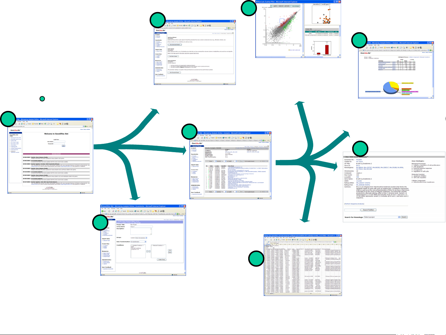
GeneSifter Overview
• Login
• Upload Tools
• Pairwise Analysis
• Create Projects
For more information
about a feature see the
corresponding page in the
User’s Guide noted in the
blue circle ( ) .
5
4
7
Upload Tools
Upload microarray data files.
33
38
63
Scatter Plot
Interactive scatter plot provides
visualization of the entire array
data set and identification of
individual genes.
Ontology Report
Summarize ontology terms
for a gene list and assess
the biological significance
of the genes within the list.
44
User Login
Access your secure
account from any
computer (PC or Mac)
with Internet access.
74
Create New Project
Create user-defined projects
with two or more groups. See
next page for project analysis
options.
Pairwise Analysis
Define two groups and apply
normalization, statistical
analysis and quality metrics to
create lists of differentially
expressed genes.
40
One-Click Gene Summary™
Provides a synopsis of the most
current information available for the
genes on your array. It includes
information from UniGene,
LocusLink, Gene Ontology terms
and more.
Export Results
Export data and gene
annotation to Excel.
Page 4
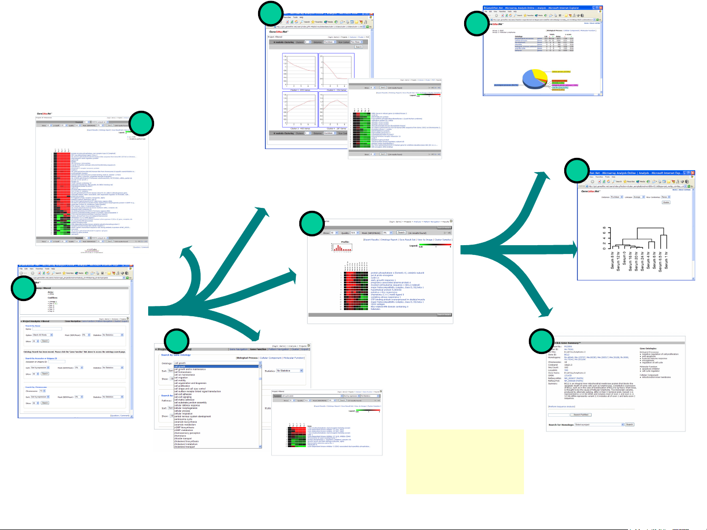
GeneSifter Overview
• Project Analysis
• Filtering
• Function Navigation
• Pattern Navigation
•Clustering
58
Filtering
Apply fold
change cutoffs,
statistical
analysis and
quality metrics
to create lists of
differentially
expressed
genes.
59
Clustering
Identify patterns of gene expression
with unsupervised clustering
functions.
54
63
Ontology Report
Summarize ontology terms
for a gene list and assess
the biological significance
of the genes within the list.
62
*
50
Project Analysis
Project analysis functions
allow analysis across all
conditions in a project.
Pattern Navigation
52
Define and identify patterns of gene
expression with supervised clustering.
Function Navigation
Rapidly identify and group genes based on
function using Gene Ontology terms.
Ontology Report, Cluster
*
Samples and the One-Click
Gene Summary are
available for all types of
project analysis.
Cluster Samples
Use hierarchical clustering to
determine the relationship of
samples based on a gene list.
44
One-Click Gene Summary™
Includes information from UniGene,
LocusLink, Gene Ontology terms
and more.
Page 5
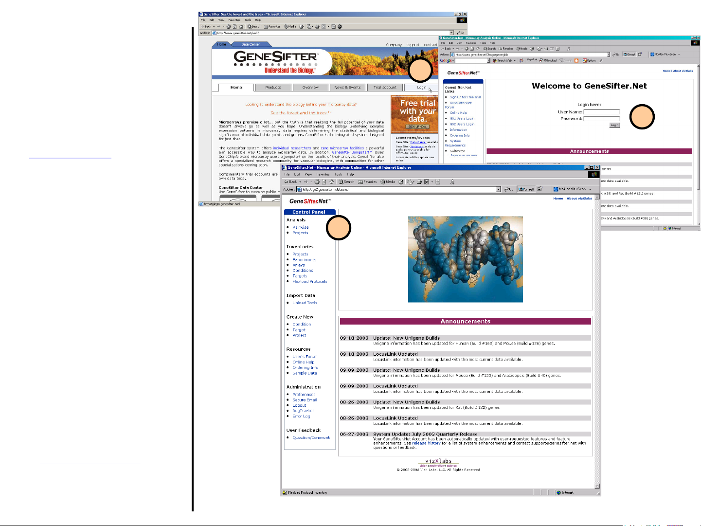
GeneSifter
Introduction and Login
Welcome to GeneSifter, the webbased microarray data management
and analysis system, which relies on
VizX Labs’ BIOME™ bioinformatics
software engine. This document gives
an overview of some of the features
available in Genesifter. To get started
from www.genesifter.net
these steps:
1. Select the Login button from the
top right corner.
2. Enter your user name and
password in their respective
prompts and click on the Login
button.
4. A successful login should show a
screen with control panel on the left
and the most recent
announcements concerning
Genesifter.
please follow
1
2
3
Genesifter Support and Sales
E-mail: support@genesifter.net
Toll-free: 1-877-WEB-GENE
Direct: 206-283-4363
Page 6
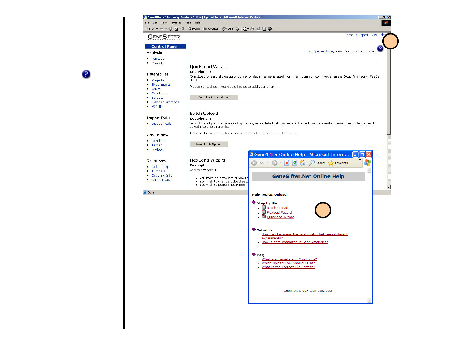
Genesifter
Online Help
Genesifter provides page-specific
online help.
1. Click on the help icon ( ) to
access page-specific help
documents. The help icon can be
found in the upper right corner of
most pages.
2. Clicking on the help icon will
open a new browser window
which will list the help available
for that particular page. Select
the document you wish to view.
1
2
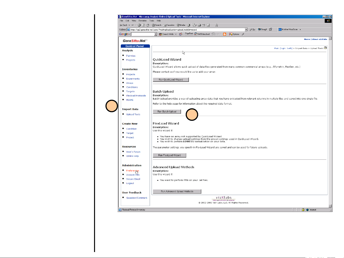
Page 7
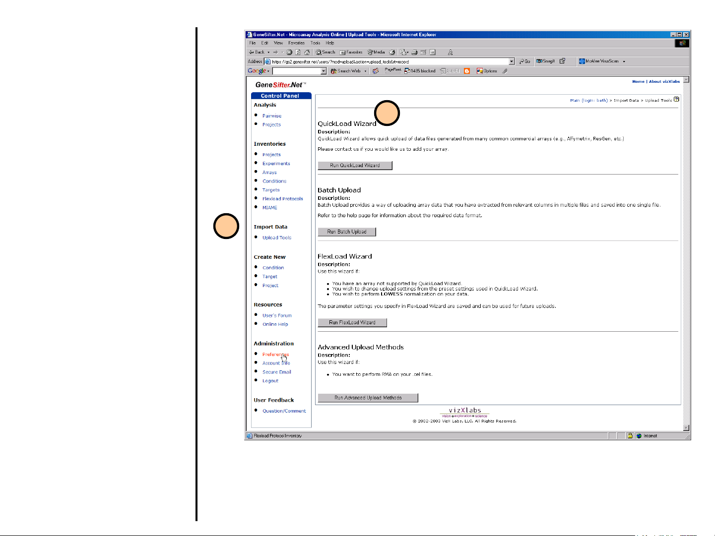
Uploading Data
Upload Tools
1. In order to upload data, select
Upload Tools from the control
panel on the left.
2. GeneSifter offers four tools to
load data. The application you
use will depend on the format
and origins of the data being
loaded. QuickLoad Wizard,
Batch Upload, FlexLoad
Wizard and Advanced Upload
Methods are further described
in the following pages.
2
1
Page 8
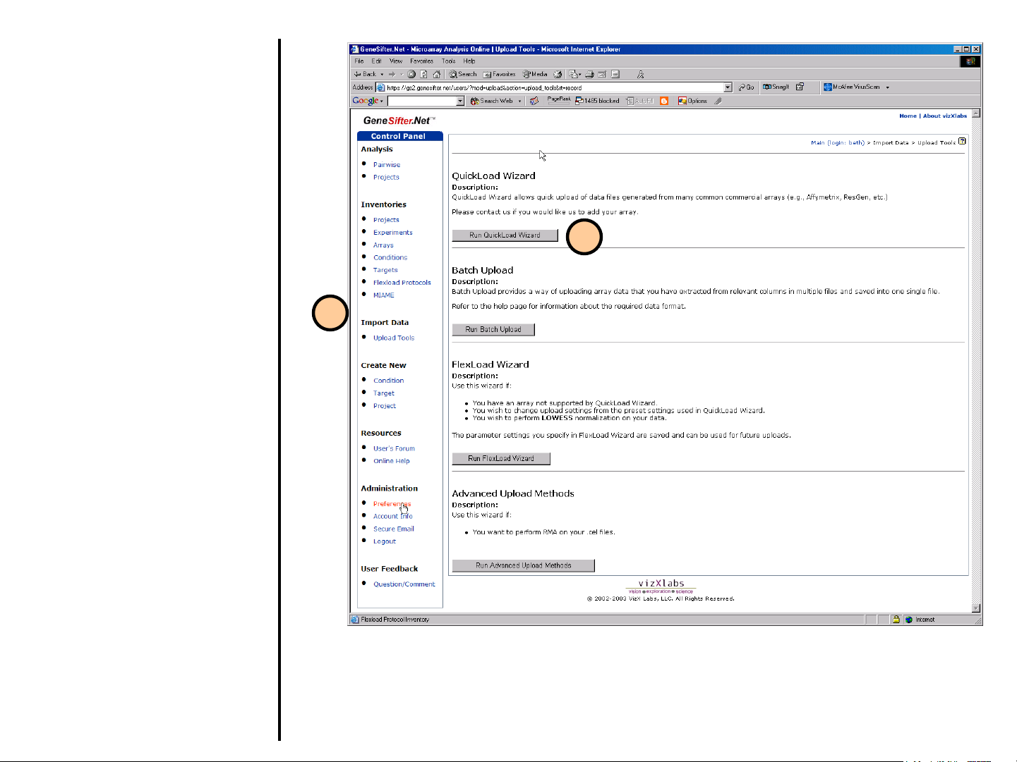
Uploading Data
Using QuickLoad Wizard
Use the QuickLoad Wizard to load your
data into GeneSifter. Supported
platforms for this tool include:
• Affymetrix (native CHP files, or CHP
files saved as tab-delimited text)
• Codelink
• Pathways™ 2 & 4
• Spot-On
• Mergen arrays scanned with
GenePix®
(all other GenePix files may be loaded
using FlexLoad)
Data Files may be archived (zipped) prior
to upload.
1. Select Upload Tools from the
control panel on the left.
2. Select Run QuickLoad Wizard from
the Upload Tools page. A new
window will guide the user in the
upload process.
2
1
Page 9
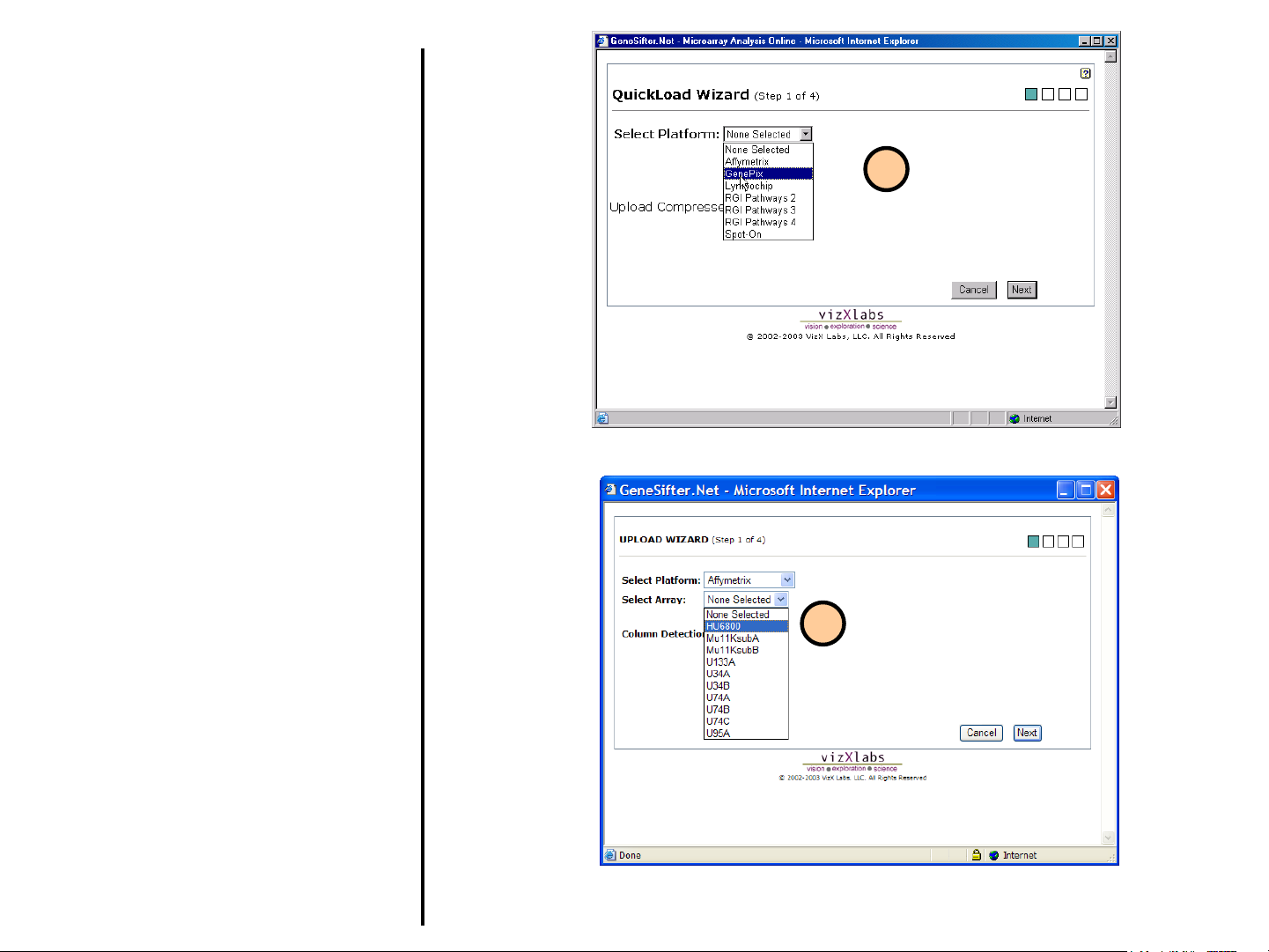
Uploading Data
Using QuickLoad Wizard (continued)
3. Select the array manufacturer or the image
analysis software used and then click the
Next button.
4. Select your array from the list of available
arrays. If your array is not listed, please
contact scientific support for
information on adding the array.After
you have selected your array, click Next.
Note for Affymetrix Users: Auto Column
Detection should work for data from MAS 5
and GCOS.
3
4
Page 10
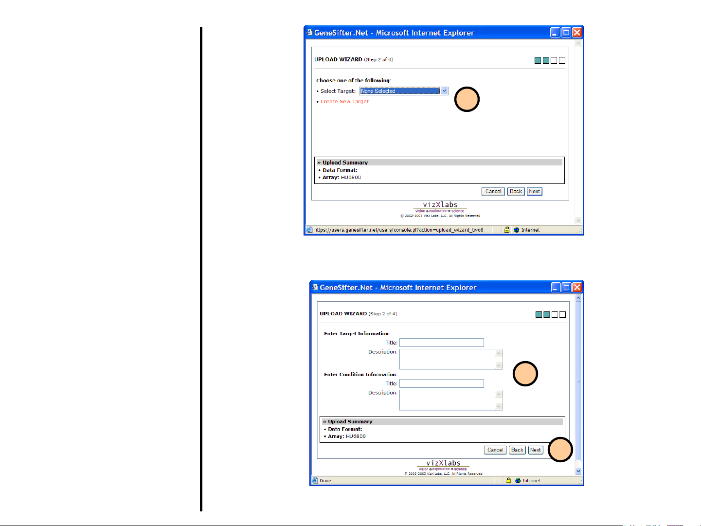
Uploading Data
Using QuickLoad Wizard (continued)
5. Now you will enter information about
the sample (referred to as “Target”)
that was hybridized to the array. If
you have already entered
information about the target, select it
from the Select Target pull-down
menu, otherwise enter your target
using Create New Target.
6. If you create a new target, you will
need to select an appropriate
“Condition” from the pull-down
menu. Otherwise, enter your
condition using Create New
Condition.
7. Select Next when you have entered
all needed information.
8. If your array has two channels,
repeat steps 5, 6, and 7 for the
second channel.
5
6
7
Page 11
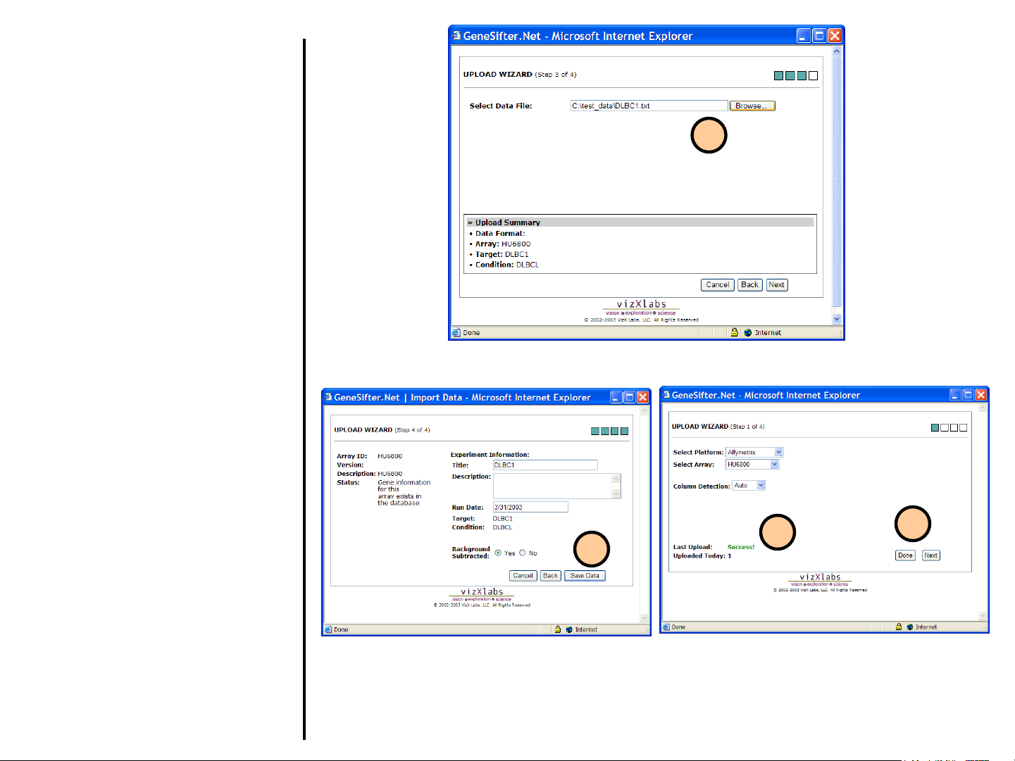
Uploading Data
Using QuickLoad Wizard (continued)
9. Select Browse and find your data file
on your local computer. Select the file
and then click the Next button to
upload the file to GeneSifter.
10. You will now see a summary of the
information you have provided. You
can enter a description for the
experiment(s) being uploaded. Select
Save Data to save the data in your
GeneSifter account.
11. When the data is successfully
uploaded, you will see Success! as the
Last Upload status. Common reasons
for failure include: data not in the
correct format, or selecting the wrong
array at step 4.
12. After saving, you can either load more
data by selecting Next or exit the
QuickLoad Wizard by selecting Done.
9
10
11
12
Page 12
Uploading Data
Using QuickLoad Wizard
Affymetrix Manual Column Detection
The Upload Wizard will automatically detect
the proper data columns for text files
generated from MAS 4, MAS 5 and GCOS. If
auto detection fails, you can use Manual
Column Detection.
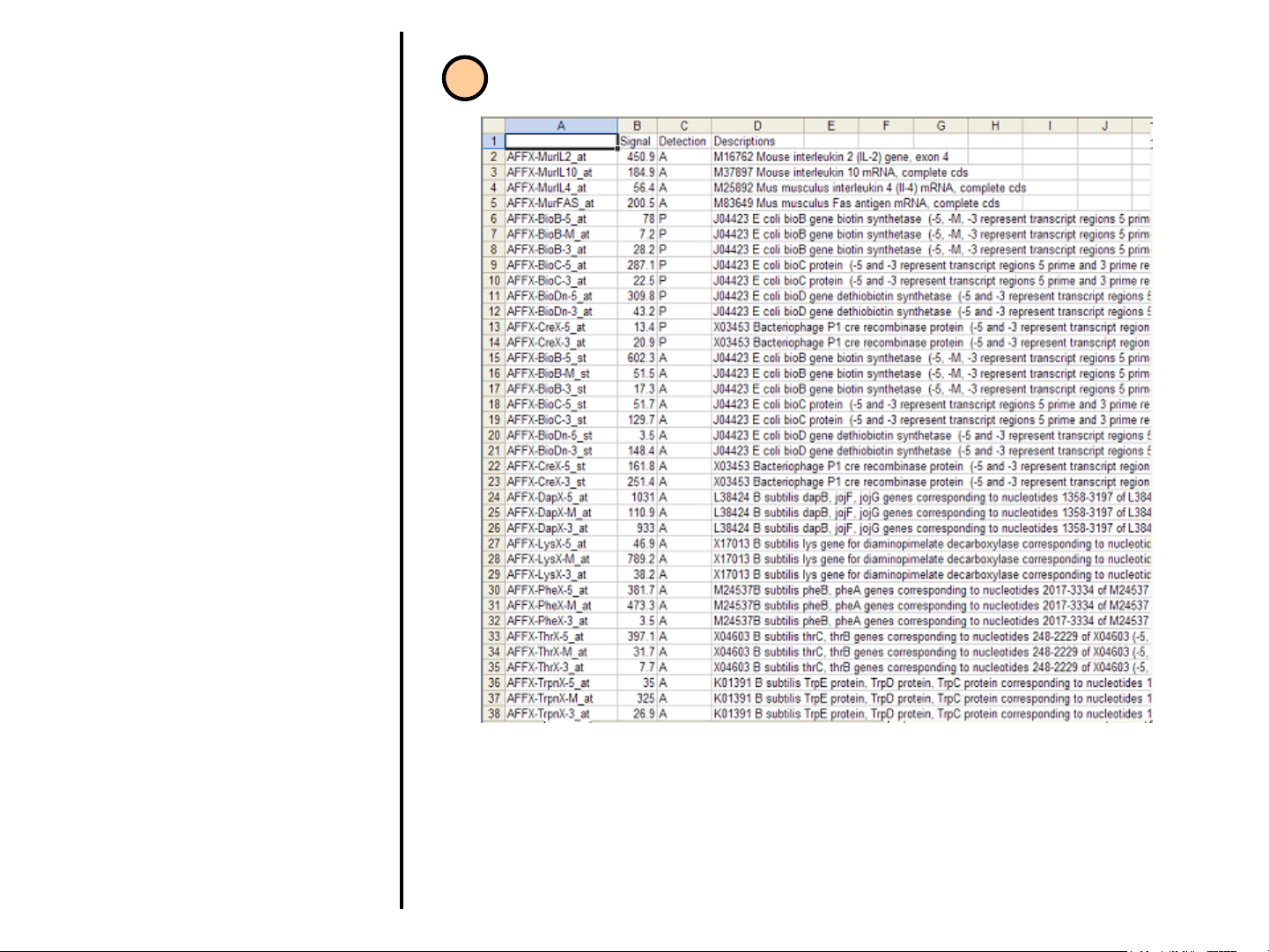
1. Affymetrix MAS 5 data format. This is
an example of a file from the U34B
GeneChip®. Formats may vary due to
differences in export from MAS 5.
Generally the first column will contain
the probeset ID. This identifies each
gene on the array. The two columns
that are needed by GeneSifter for
analysis are the columns containing the
signal and detection value for that
probe set. In this example, column B,
which is labeled Signal, contains the
derived signal value and column C,
labeled Detection, contains the quality
value. There may be additional
columns present in a data file and the
heading for the signal and quality
values may be different than what is
presented here. In general the signal
column will either be labeled Signal or
will have the word Signal at the end of
the column name. This column can
contain both positive and negative
numbers. The quality column will
generally be labeled Detection or will
have the word Detection at the end of
the name. This column will contain the
letters A, M and P.
1
Page 13
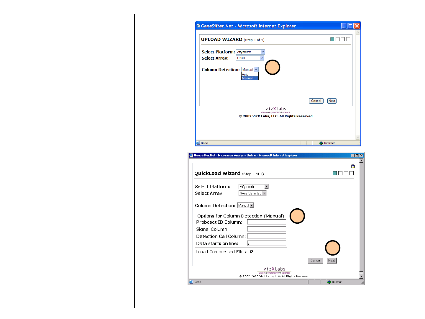
Uploading Data
Using QuickLoad Wizard
Affymetrix Manual Column Detection
(continued)
2. Select Run QuickLoad Wizard as
usual (see preceding description).
Select Manual from pull-down menu.
3. Enter information about columns in the
data file. In the sample file the
probeset ID is in the first column
(column A), the signal is in column B
and the detection call value is in
column C, so A would be entered for
Probeset Column, B would be entered
for Signal Column and C would be
entered for Detection Call Column. In
the sample file the data begins on the
second line of the file so 2 is entered
for Data starts on line.
4. Select Next and continue as usual for
QuickLoad Wizard. The setting will
be saved and used to correctly upload
the data.
2
3
4
Page 14
Uploading Data
Using Batch Upload
Use Batch Upload to load multiple data
sets stored in a spreadsheet as a tabdelimited text file. Note: See step 7 for a
description of required file format.
1. Select Upload Tools from the
control panel on the left.
2. Select Run Batch Upload.
1
2
Page 15

Uploading Data
Using Batch Upload (continued)
3. Enter a name and description for
the array you are uploading. The
pull-down menu has options for
the type of data being loaded
including:
Use Affymetrix Probeset IDs –
use if the first column of your file
contains Affymetrix Probeset IDs
instead of GenBank accession
numbers.
This File is a GEO Data Set –
use if you downloaded data from
GEO as a GEO dataset.
Use CodeLink Quality Values –
use if your file has the CodeLink
flags G, M, L.
4. Browse your computer to find the
file containing your data. Use the
Select Array pull-down if you
have previously loaded data from
this array and you wish to add to
that data set.
3
4
5
5. Select Upload Data.
6. Data uploaded. You can either
exit Batch Upload by selecting
Done or select Upload More
Data.
6
Page 16
Uploading Data
Using Batch Upload (continued)
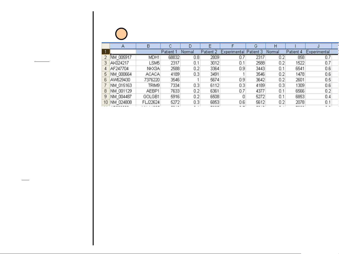
7. The file to be loaded must be a tabdelimited text file (txt). GeneSifter
does not accept Excel spreadsheets
(xls).
The first column
figure) should contain an identifier
for that gene. Accepted identifiers
are:
Accession Number
IMAGE Clone ID
Affymetrix Probeset IDs
The second column (Column B) is
for an internal identifier. This is left
to the discretion of the user and can
be left blank.
The next 2 columns contain the
intensity (Column C) and quality
values (Column D) for that gene in
the first experiment to be loaded.
Additional experiments are added in
the same way (one column for
intensity, one for quality).
(Column A in the
7
The first row
A: This cell can be empty.
B: This cell can be empty.
C: Target name for Experiment #1.
D: Condition for Experiment #1.
E: Target name for Experiment #2.
F: Condition name for Experiment #2,
etc.
must contain this information.
Page 17
Uploading Data
Using Batch Upload (continued)
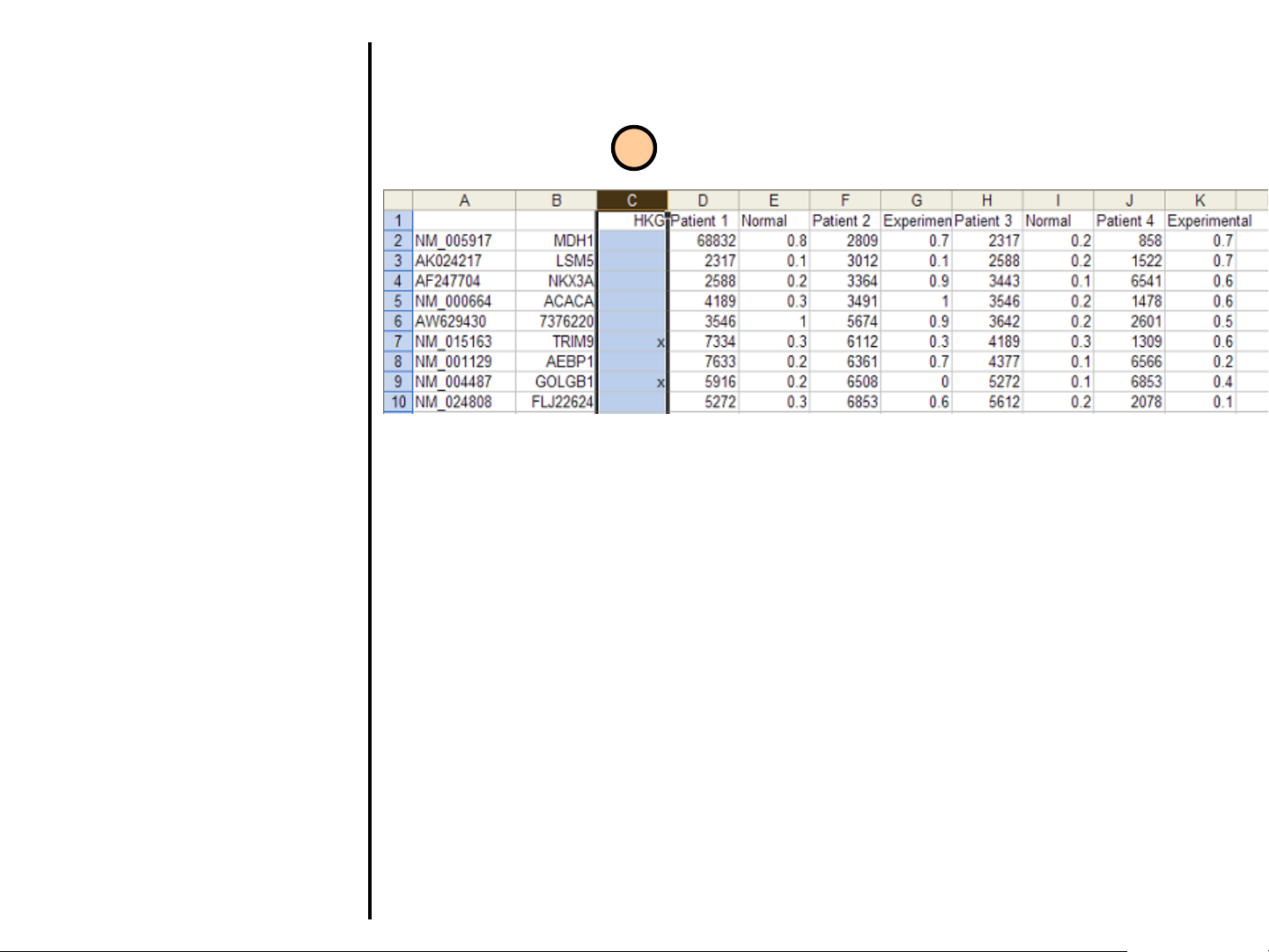
8. File format for Batch Upload using
housekeeping genes. The format is
the same with one exception: the
third column must be labeled HKG
(housekeeping genes). The genes
that are designated as
housekeeping should be marked
with an x in this column. The
intensities and quality values should
follow as stated for Batch Upload
without housekeeping genes.
In this example the genes in rows 7 and 9
(TRIM9 and GOLGB1) have been
designated as housekeeping genes.
8
Page 18
Uploading Data
Using FlexLoad Wizard
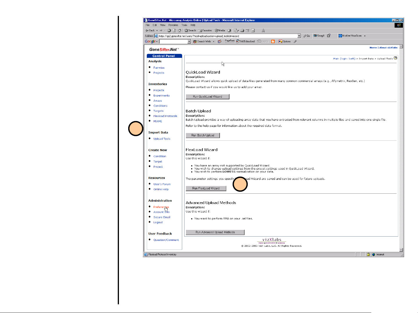
Use the FlexLoad Wizard to load data in
GeneSifter if the array you are using is
not included in the QuickLoad Wizard.
Familiarity with the layout of your files is
advised before going any further. You will
be asked:
• to provide information about the file
structure, e.g. what column
describes absolute intensity,
background intensity, etc.
• how you want the data transformed,
e.g. preserve channel intensities or
express as a ratio of the two
channels.
• how you want the data normalized,
e.g. LOWESS
1. Select Upload Tools from the
control panel on the left.
2. Select Run FlexLoad Wizard.
.
1
2
Page 19
Uploading Data
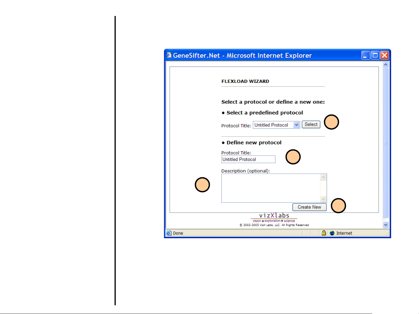
Using FlexLoad Wizard (continued)
1. The Protocol Title is the name
given to a protocol (i.e. the settings
for a specific type of file to be
uploaded). You can select a
protocol you have already
generated or create a new one.
2. If creating a new protocol, replace
“Untitled Protocol” with a Protocol
Title.
3. Enter an optional Description for
the protocol.
4. Click on Create New to begin the
creation of a new protocol.
1
2
3
4
Page 20
Uploading Data
Using FlexLoad Wizard (continued)
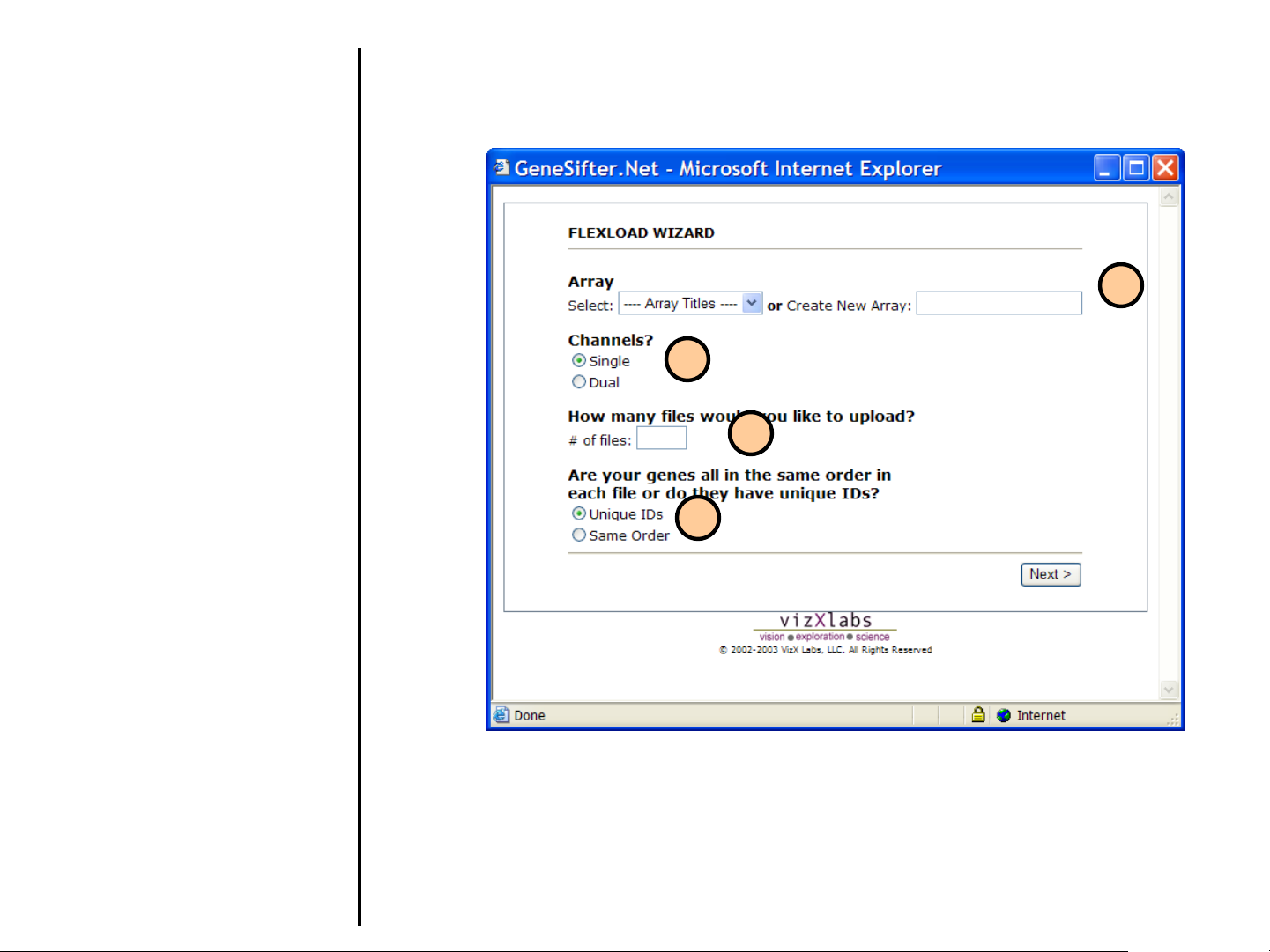
5. If you previously loaded the array
into your account, select it from the
menu list. Alternatively, if you are
creating a new protocol, enter the
name of the array in the Create New
Array field.
6. Select the number of Channels.
7. Enter the number of files you will be
uploading (the maximum allowed at
any one time is 30).
8. If you know that the genes are all
listed in the same order in every file
(experiment) then select Same
Order.
If you select Unique IDs, FlexLoad
will not assume identical gene order
in each file, but instead will utilize a
supplied unique identifier. If Unique
IDs is selected, every ID for that
array must be unique and there
cannot be any blank data rows.
Ideally, you should use a GenBank
Accession Number or an Image
Clone ID as the Unique ID to assist
in populating the One-Click Gene
Summary.
5
6
7
8
Page 21
Uploading Data
Using FlexLoad Wizard (continued)
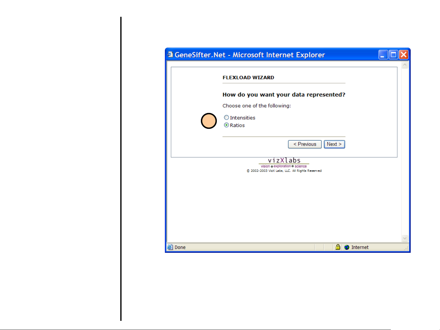
If your data has two channels, from Step 6:
9. Select how you want your data
represented:
Intensities
Data for each channel will be stored
separately in GeneSifter.
Ratios
Generates a ratio of the intensities of
the red and green channels.
GeneSifter only saves the ratio to your
account.
9
Page 22
Uploading Data
Using FlexLoad Wizard (continued)
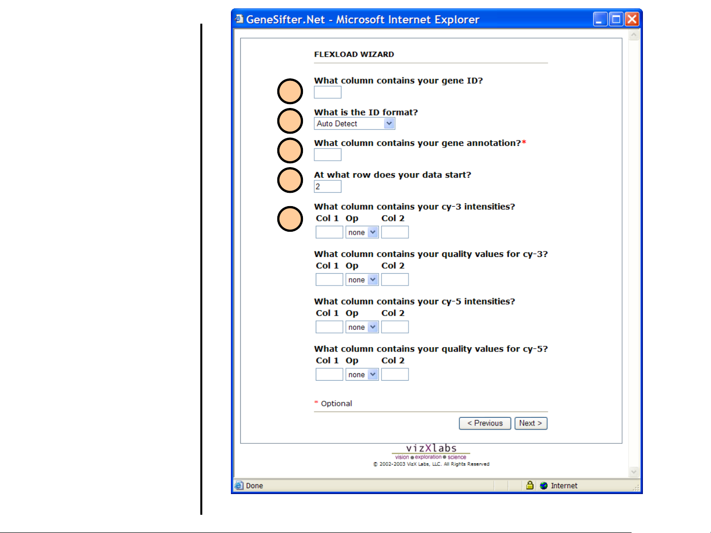
10. Provide the column number or letter
that contains the gene ID.
11. Identify the type of gene ID by
selecting either Auto Detect,
Accession Number, IMAGE Clone
ID, or Other. If Accession Number
or IMAGE Clone ID is selected and
the data file contains other identifiers
or blank rows, errors may occur. In
general Auto Detect should be
used.
10
11
12
13
12. Optionally, indicate the column
number for gene annotation, if
available.
13. Indicate the row number where the
intensity data begins. Do not include
the column headings.
14. Provide the column numbers that
contain the respective data. For
example, if your data file contains
the cy3 intensity in column 8 and
column 10 contains the background,
enter 8 for Col 1 and 10 for Col 2 to
specify these values for the cy-3
intensities.
Op refers to the operation to perform
between the two values. Op may be
used to subtract background, or take
the ratio of foreground/background
for quality control purposes. It is not
necessary to enter any value for Op,
or Col 2.
14
Page 23
Uploading Data
Using FlexLoad Wizard (continued)
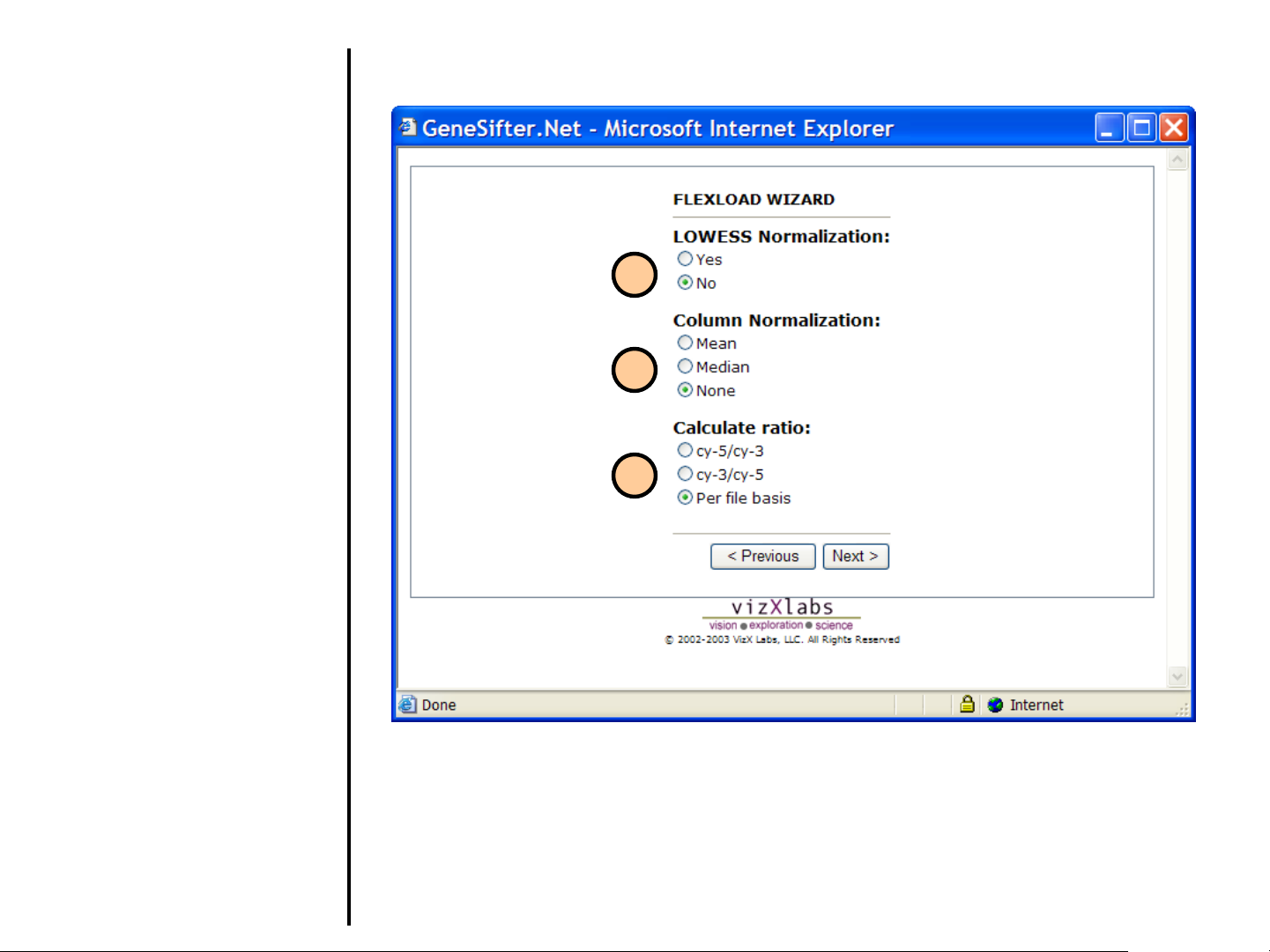
This window appears only if
you chose Ratios in Step 9.
15. Perform LOWESS Normalization
on the data.
16. Select how you want to normalize
the data.
17. Method for calculating the ratio of
intensities. Per file basis allows
you to take into account any dye-
swap experiments you may have.
15
16
17
Page 24
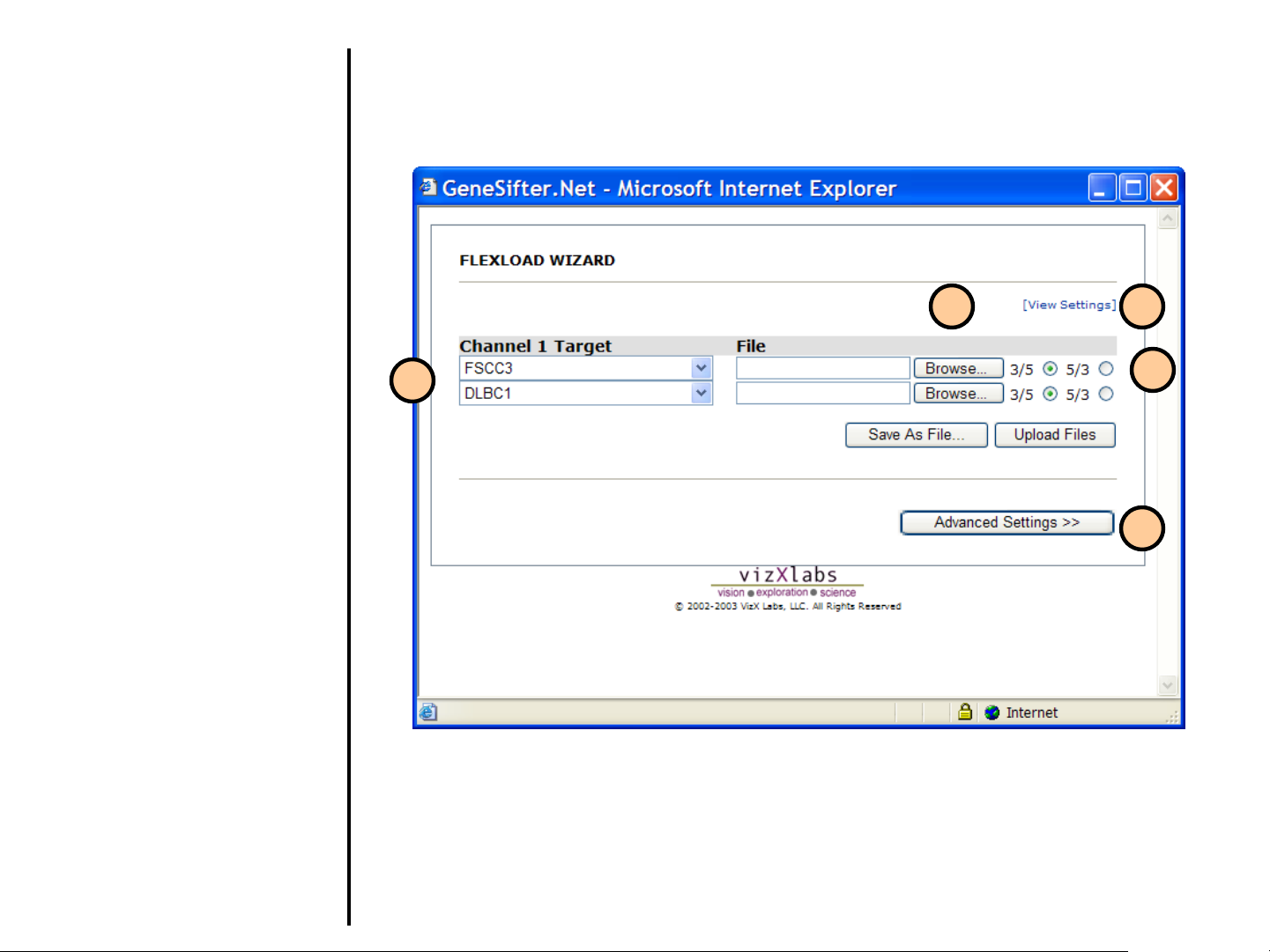
Uploading Data
Using FlexLoad Wizard (continued)
18. If your targets already exist, you
can select them from the pulldown menu. If you need to
create new targets, use
Advanced Settings.
19. Select Browse to upload the
file(s). If you were uploading
more files, additional rows would
be present. In this screen, two
files are being uploaded.
19
21
20. For two-color arrays, if Per file
basis was selected in step 17,
indicate whether you want the
ratios to be cy5/cy3 (5/3) or
cy3/cy5 (3/5).
21. A summary of parameters that
have been previously selected
can be viewed.
22. Select Advanced Settings if
you need to enter the target and
condition information, or to
change the number of files being
loaded.
18
20
22
Page 25
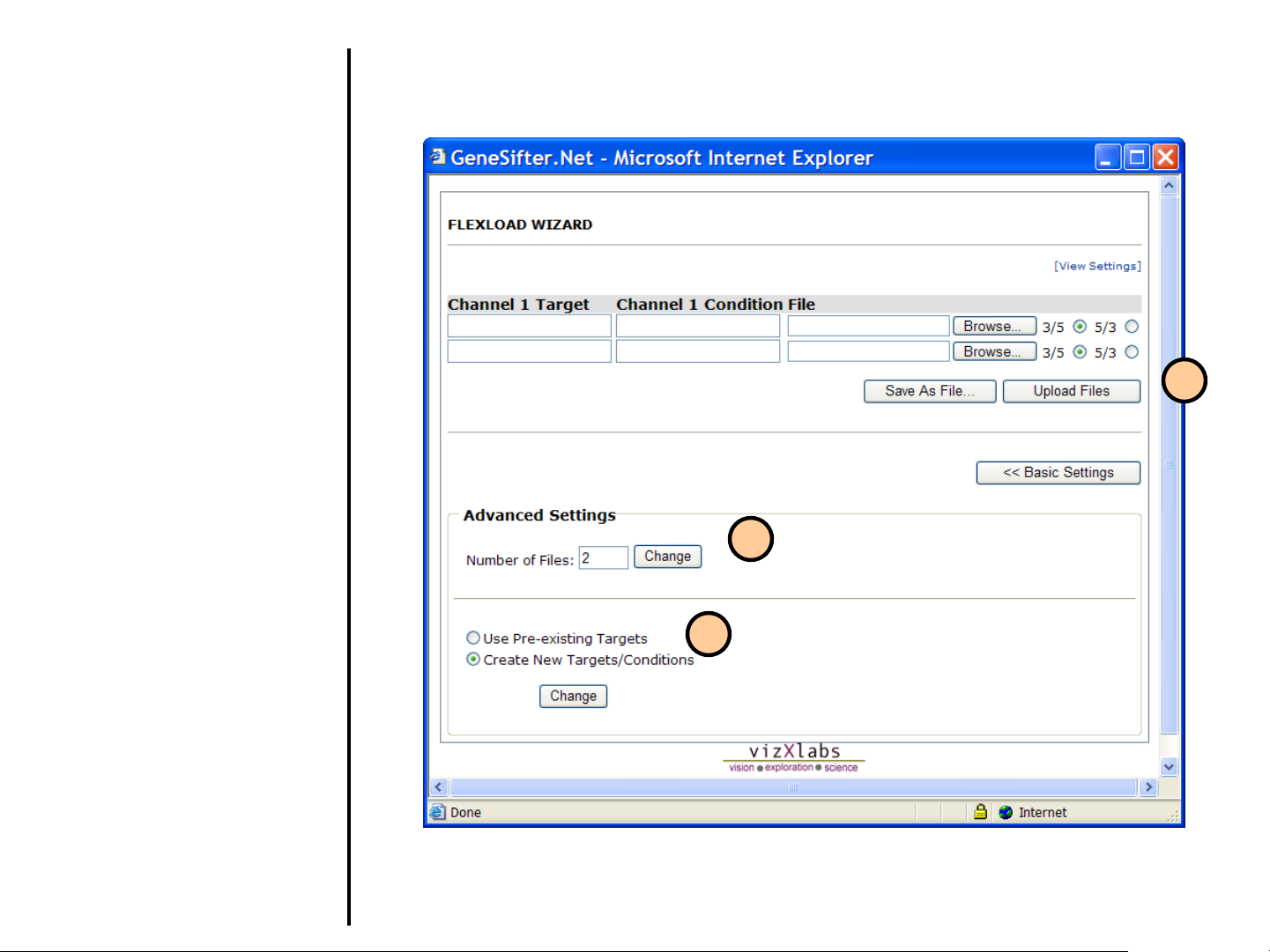
Uploading Data
Using FlexLoad Wizard (continued)
23. Upon selecting Advanced
Settings, you can change the
number of files to be loaded.
24. You also have the ability to “Create
New Targets/Conditions”. Enter
target and condition information for
each file to be loaded in the top
portion of the screen. Otherwise,
select “Use Pre-existing Targets”.
25. You can save the output as a text
file formatted for Batch Upload by
selecting Save as File or load it
directly into GeneSifter by selecting
Upload Files
.
25
23
24
Page 26
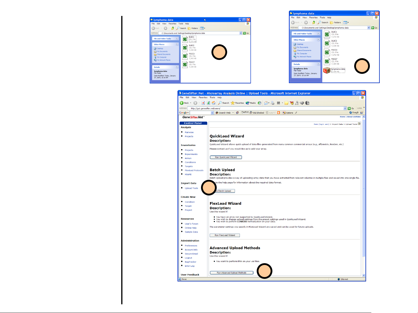
Uploading Data
Advanced Upload Methods
Robust multi-array average (RMA) is a
method for deriving expression
measurements from the probe level data
contained in an Affymetrix CEL file.
GeneSifter users have the option to
perform RMA or GC-RMA during the
upload of CEL files. The normalized data
is saved in the user’s account for further
analysis.
1. Locate the Affymetrix .CEL files
you want to load on your local
computer.
2. All the files to be uploaded and
transformed using RMA need to
be compressed into a single ZIP
file for upload.
3. Select Upload Tools from the
Control Panel.
4. Click on Run Advanced
Upload Methods to begin.
1
2
3
4
Page 27
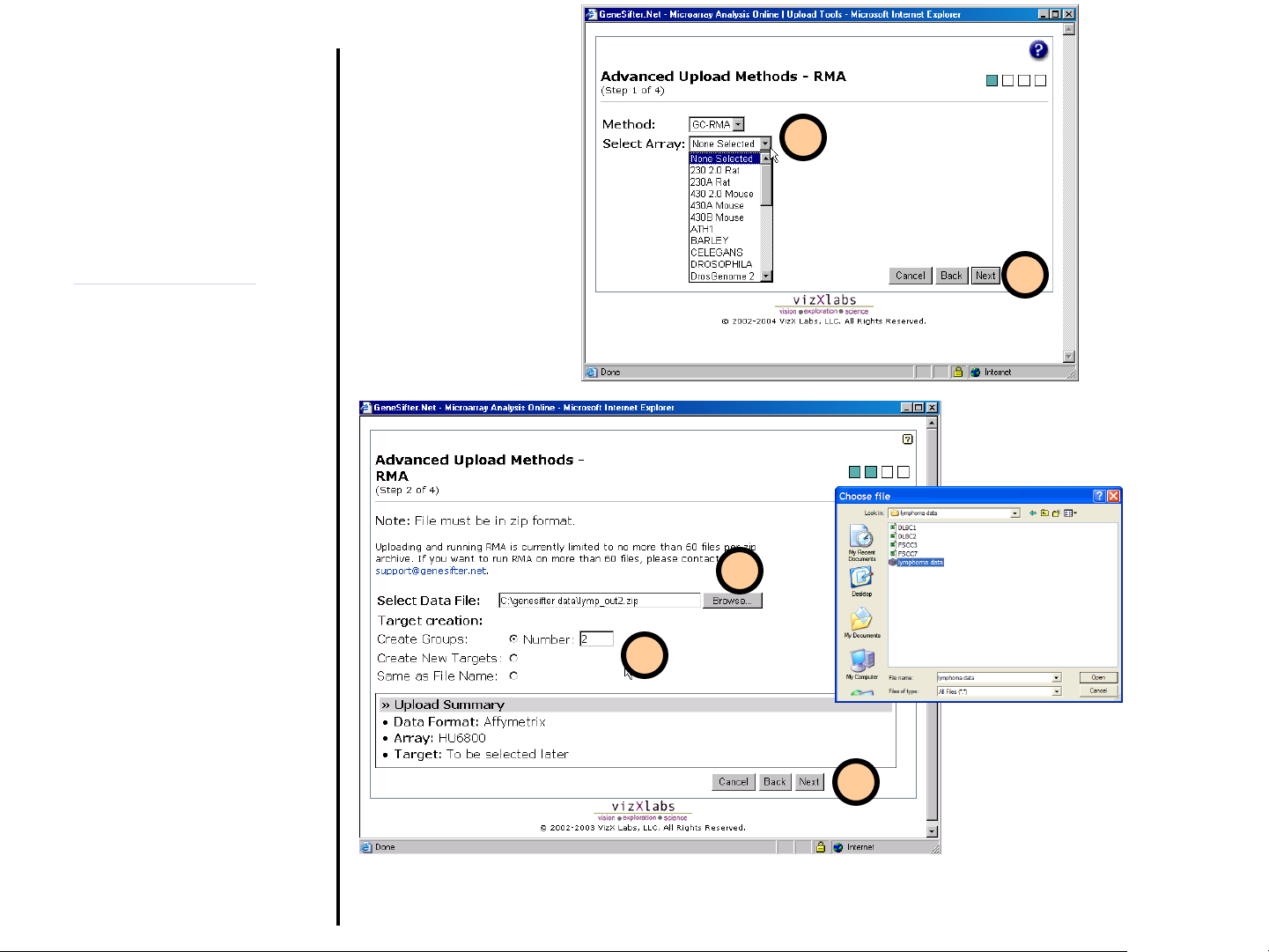
Uploading Data
Advanced Upload Methods
(continued)
5. Select the normalization
method. Select the type of
Affymetrix array used in your
experiments. If your array is
not listed, please contact
scientific support
(support@genesifter.net
help loading your array format.
6. Click the Next button to
continue.
7. Click Browse to locate the .zip
archive containing the CEL files
on your local disk. Please note
that all the files to be loaded
need to be contained within a
single .zip file.
8. Choose how you want to create
targets and conditions for the
loaded files.
9. Click Next to continue.
) for
5
6
7
8
9
Page 28

Uploading Data
Advanced Upload Methods
(continued)
10. Enter information about the
data set, including a title and
description. If you chose to
create groups for your
experiment, you will now be
prompted to create titles for
each group.
11. Click the radio buttons to place
experiments into the
appropriate group (in the
example shown experiments 3
and 4 are assigned to group 2
– FL). You may also change
the names for the experiment
and target/sample at this point.
Click Next to continue.
12. GeneSifter will now complete
the uploading and
transformation of the data. If
the upload is Successful, you
can click Done to exit the
wizard. Any error messages
will also be displayed here.
Please contact us if you
receive an error message and
would like help resolving the
problem.
10
11
12
Page 29

MIAME
MIAME is the Minimum Information
About a Microarray Experiment that
should be associated with public
microarray data. Genesifter can store
MIAME, by providing information
through a user-friendly interface. The
Genesifter V1.5 MIAME interface is
designed for extraction and labeling
protocols. Subsequent versions will
have an interface where more MIAME
can be provided.
1. Access the MIAME interface by
clicking on MIAME under Inventories.
2. If MIAME isn’t present, turn it on under
Preferences.
3. Under Preferences > General, turn
MIAME on.
4. A list of all the MIAME Extraction,
Labeling and Sample Treatment
protocols created are shown under
MIAME >> Inventories.
3
4
5
1
5. Create a new MIAME protocol by
selecting the appropriate type in
Create New.
6. Provide a title for the MIAME protocol
(the protocol in this case PCR
Protocol is the title).
7. Provide information about the protocol
by selecting values in the pull-down
menus. If a suitable value is not in a
menu list, it can be created in the
other text box. This value will become
part of the menu list when the protocol
is created.
2
6
7
Page 30

MIAME
(continued)
8. Many protocols may have
additional information. This can be
included in the Full Protocol
Description text box (e.g.
providing a complete PCR
protocol).
9. Select Create to save a new
MIAME protocol.
10. The newly created MIAME object
should appear under
MIAME>Inventories.
11. To edit or delete a MIAME
protocol click on the protocol and
select the appropriate button.
8
9
10
11
11
Page 31

MIAME
(continued)
12. To associate MIAME information with a
target click on Targets under
Inventories, choose and click a
Target.
13. Click on Edit and select the
appropriate MIAME object.
Note: All Experiments that have this
target, will automatically be associated
with the newly created MIAME object.
12
7
7
13
Page 32

Pairwise Analysis
Set-Up
Pairwise Analysis allows you to set up
two groups of data and look for genes that
are differentially expressed between the two
groups.
1. Select Pairwise under the Analysis
heading from the Control Panel.
2. A list of available arrays will show on
the screen, along with a description if
it was entered upon upload.
3. Select the Analyze icon ( ) to
perform a pairwise analysis for a
particular array.
4. Upon selecting the Analyze icon, a
list of experiments performed using
that array is displayed. The
experiments are grouped by
condition. Select the experiments for
Group 1 by checking the
corresponding boxes in the Group 1
column.
1
2
3
6
4
5. Likewise, select the experiments for
Group 2.
6. For an overview of experiment details,
select the Document icon ( ).
7. You can now select Analysis
Settings parameters to be used in the
Pairwise Analysis.
5
7
Page 33

Pairwise Analysis
Set-Up (continued)
8. Select a normalization method from
the Normalization pull-down menu.
Options are All Mean, All Median or
None.
9. Select a method for determining
reliability and consistency between
replicates of each gene from the
Statistics pull-down menu. Options
include t-test (two tailed, unpaired
Student T), Welch’s t-test,
Wilcoxon (non-paramteric) or none.
10. Select Threshold value from the
pull-down menu. This number sets
the threshold for display of up or
down regulation (e.g. setting to 1.5
would select only genes that are
differentially expressed by at least a
factor of 1.5 in one group compared
to the other).
11
8
9
10
11. You can select a Quality cutoff
value for your data. This is optional
and the value is calculated
differently for different array types.
Page 34

Pairwise Analysis
Set-Up (continued)
12. You can choose to display Upregulated and/or Down-regulated
genes.
13. The Data Transformation field
allows users to specify the following:
• The data should not be log
transformed.
• The data should be log
transformed for analysis.
• The incoming data has
already been log
transformed prior to upload.
Note: Transformation is to log
base 2.
13
12
14. Perform your analysis by selecting
the Analyze button.
14
Page 35

Pairwise Analysis
Advanced Settings
15. If Advanced Pairwise Settings
was turned on in the Preferences
section, additional parameters are
made available for use in analysis.
16. Select an Upper threshold if you
would like to set an upper cutoff for
the fold differences between
Groups 1 and 2.
17. You may decide to include a
Correction factor for multiple
testing. Options include
Bonferroni (step adjusted p-value),
Holm (step down adjusted p-value),
Benjamini and Hochberg (false
discovery rate), Westfall and
Young - maxT or None. If you
select a correction method, you
must also be performing a statistical
test.
18. Perform your analysis by selecting
the Analyze button.
15
16
17
18
Page 36

Pairwise Analysis
Results
1. After submitting pairwise
comparison analysis parameters, a
list of differentially expressed genes
is returned. The genes are ordered
by ratio, listing those genes which
are most differentially expressed at
the top of the list.
2. The colored arrow indicates whether
expression is higher (red up arrow)
or lower (green or blue down arrow;
color dependent on Preferences) in
Group 2 compared to Group 1.
1
3. The total number of genes (results
found) is indicated next to the
Search button. The default gene list
display is twenty genes per page; to
show more, increase the number in
the Show pull-down menu and
select Search.
Sort by p-value
If a statistical test was included in
the pairwise comparison, the list can
be sorted by p-value from the Sort
By pull-down menu and then
selecting the Search button. Genes
will be sorted by ascending p-value.
If multiple corrections, have been
applied, that p-value is used.
p Cutoff
The user can view results that are
less than or equal to the selected p
cutoff. A statistical test (t-test,
Welch’s t-test or Wilcoxon) must
be performed in order to use the p
Cutoff.
3
2
Page 37

Pairwise Analysis
Results (continued)
4. Select the Export Results link to
export the results of the pairwise
comparison. Depending on your
Preferences, data can be exported
directly into Excel or saved as a tabdelimited text file.
5. To view the One-Click Gene
Summary about any gene in the list,
select the gene name.
6. To view more genes within the list,
click on the [range] hyperlink.
4
5
6
Page 38
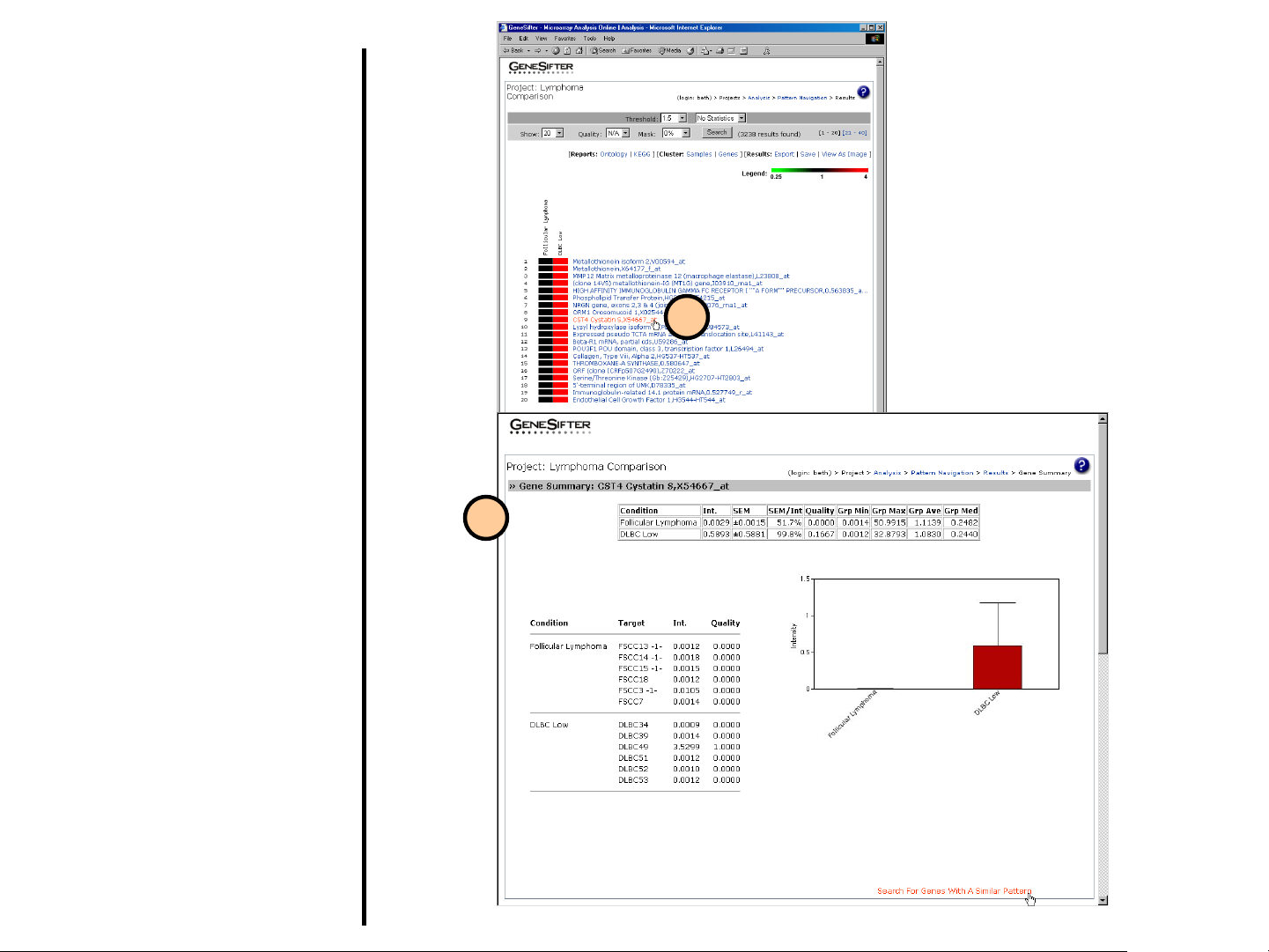
One-Click Gene
Summary™
The One-Click Gene Summary is a
powerful feature in GeneSifter that
provides a synopsis of the most current
information for each gene on an array.
Each gene within a gene list has
additional annotation, curated from
various data sources.
1. Click on a gene of interest from the
results list.
2. A gene summary appears in a new
window. Within the upper panel, the
mean expression values for each
condition (group) are displayed, as
well as the raw data for the individual
arrays. A link allows you to “Search
For Genes With a Similar Pattern”.
1
2
Page 39

One-Click Gene
Summary™
(continued)
3. In the lower pane of the One-Click
Gene Summary:
Accession No
This ID is from the GenBank database.
Clicking on it will display the GenBank
record. Specific arrays may have
additional IDs, such as Probe Set ID for
Affymetrix (links to NetAffx™).
Cluster ID
This ID is from the UniGene database.
Clicking on it will display the full UniGene
record.
UG Title
The title of the gene cluster in UniGene
that contains this gene.
Gene ID
This is the gene Nomenclature ID as
curated by the Nomenclature Committee.
Clicking on it will display the GeneCard™
record for the gene.
3
Homologene
Lists genes from the same or other
organisms that show high sequence
similarity.
Chromosome
Indicates the chromosome on which the
gene is present (from UniGene).
Page 40

One-Click Gene
Summary™
(continued)
Cytoband
The cytogenic marker to which the gene
belongs (from UniGene).
Seq Count
The number of sequences in the UniGene
cluster.
LocusLink
The ID from the LocusLink database. By
clicking on it, the LocusLink entry is
displayed.
Gene Name
The gene name (taken from LocusLink).
OMIM™
ID number from the OMIM database.
Clicking on this link will display the OMIM
record for this gene.
3
RefSeq mRNA
ID from the NCBI Reference Sequence
database of comprehensive, nonredundant mRNA transcripts. If you click
on (FASTA) the sequence appears in
FASTA format in a new window.
RefSeq Prot
The ID is from the NCBI Reference
Sequence database of comprehensive,
non-redundant protein sequences. If you
click on (FASTA) the sequence appears
in FASTA format in a new window.
Page 41

One-Click Gene
Summary™
(continued)
Summary
A short paragraph summarizing what is
known about the function of the gene (from
LocusLink).
Gene Ontologies
Gene Ontology™ terms for the gene (from
LocusLink). Each term is hyperlinked to
show the GO hierarchy.
KEGG Pathways
A link to the Kyoto Encyclopedia of Genes
and Genomes (KEGG). It provides
pathway information for gene products.
PubGene
3
Link to the PubGene
providing a tool to explore both literature
and sequence co-association networks
(from PubGene
Tools).
Additional Search Features:
- Perform Sequence Analysis
blastn, blastx and primer design tools
- Search PubMed
Use either the Gene ID(default) or enter
another term to search PubMed.
- Search for Homologs
Search within other projects for
homologous genes.
™ Network Browser
™ Web database and
Page 42

BLAST®Analysis
A BLAST search can be performed on any
gene sequence within the secure GeneSifter
environment.
1. Click on a gene from the results list of
either pairwise or project analysis.
2. At the bottom of the One-Click Gene
Summary window, click on Perform
Sequence Analysis.
3. A new window will open with the
selected sequence pasted in a form
ready for BLAST analysis. Select the
type of BLAST search to perform
(blastn or blastx) from the buttons at
the bottom left corner of the window.
4. To determine suitable primers for a
selected nucleotide sequence, there is
a link to primer3, again with the
sequence already loaded into the
application.
1
Note: Use blastn to BLAST the sequence
directly against a nucleotide database. Use
blastx to BLAST against a protein
database. The latter works by translating
your nucleotide sequence in all six reading
frames (three for each direction) and
blasting each result against the protein
database.
2
3 4
Page 43

Ontology Report
The Ontology Report is available for any gene list
created in GeneSifter. In a gene list from either
Pairwise or Project analysis, select the link for
Ontology Report in the upper right corner.
1. Gene Ontology (GO) terms are divided
into three general categories. The
default display will be the Biological
Process ontologies. To see the report
for either Cellular Component or
Molecular Function, select the
appropriate link.
2. You can view the data as an Ontology
Report or Z-score Report.
3. Ontology summary table. Summarizes
GO terms for genes in the list (see
number 5-8 for additional details).
4. Pie chart of ontology distribution.
Summarizes the frequency of GO terms
listed in summary table (see number 9
for details).
1
2
3
4
Page 44

Ontology Report
(continued)
5. Genes link displays the genes in the list
that correspond to the current ontology.
6. GO link displays the Gene Ontology tree
structure for a GO term.
7. Ontology Totals:
List – displays how many genes with the
specific ontology term are in the
gene list. For pairwise analysis
this list is further divided into upregulated (red arrow) and downregulated (green arrow).
Array – displays how many genes with the
specific ontology were measured
in the comparison. Typically, this
is the number of genes of that
specific ontology on the array
being analyzed.
5 6
7
8
8. z-score. Indicates whether each GO term
occurs more or less frequently than
expected. Extreme positive numbers
(greater than 2) indicate that the term
occurs more frequently than expected,
while an extreme negative number (less
than -2) indicates that the term occurs less
frequently than expected (see number 10
for calculation details).
Page 45

Ontology Report
(continued)
9. The pie chart of ontology term
distribution is a display of the frequency
of GO terms in the summary table.
10. z-score calculation:
R = total number of genes meeting
selection criteria
N = total number of genes measured
r = number of genes meeting selection
criteria with the specified GO
term
n = total number of genes measured
with the specific GO term
9
10
Page 46

Z-score Report
The Z-score Report is generated from the same
data as the Ontology Report. It displays those
GO terms that have a z-score greater than 2, or
less than -2. In a z-score report generated from a
Pairwise analysis, a score is calculated for both
up and down-regulated genes. Only one of
these scores needs to pass to be included in the
cut off.
1. Click on Z-score Report to list the
genes by z-score
2. The default view sorts the terms
according to the ontology that is most
highly represented within the list. Click
on List to sort or re-sort the list in this
fashion.
3. Alternatively, to sort the list by z-score
in:
a) Pairwise - Click on the arrows.
1
2
3a
3b
b) Projects - Click on z-score.
Page 47

Pathway Report
The Pathway Report is available from any gene list
created in GeneSifter by selecting the link for
Reports | KEGG.
Note: The pathway report is currently available only
for human microarrays. The pathway source is from
the Kyoto Encyclopaedia of Genes and Genomes
(KEGG).
1. All pathways from the gene list are
shown.
2. The Genes link displays all genes from
the list that are associated with the
corresponding pathway.
3. The KEGG link displays the
corresponding pathway and highlights
the appropriate gene(s) from the gene
list.
4. Totals:
List – displays how many genes in the
gene list belong to a pathway.
For pairwise analysis this list is
further divided into up-regulated
(red arrow) and down-regulated
(green arrow).
Array – displays how many genes
belonging to a pathway were
measured in the comparison.
Typically this is the number of
genes of a pathway that are
present on the array being used.
1
32
4
Page 48

Pathway Report
(continued)
5. z-score. Indicates whether a pathway
occurs more or less frequently than
expected. Extreme positive numbers
(greater than 2) indicate that the term
occurs more frequently than expected,
while an extreme negative number (less
than -2) indicates that the term occurs
less frequently than expected.
6. z-score calculation:
R = total number of genes meeting
selection criteria
N = total number of genes measured
r = number of genes meeting selection
criteria with the specified
pathway
n = total number of genes measured
with the specific pathway
5
6
Page 49

Scatter Plot
After performing a pairwise comparison, the
data can be viewed as a Scatter Plot with
the log intensities for Group 1 plotted against
the log intensities for Group 2. This plot
displays the data for all of the genes and
color codes the differentially expressed
genes. The first time Scatter Plot is
selected, there may be a few second delay
due to the initial intensive calculation.
1. Select Scatter Plot from the
Pairwise Comparison Results
page. A new window will be
displayed.
2. Clicking print plot in the blue control
box will print the scatter plot or save
it to a file.
3. The middle toggle line button
allows the user to view/hide the
identity line.
4. All the data for that comparison will
be displayed on the plot (if multiple
experiments were included for a
group, the log of the mean intensity
for the group is plotted). Red spots
represent genes that are more highly
expressed in Group 2 and green
represents genes that are expressed
at a lower level in Group 2. Gray
spots represent genes that are not
differentially expressed based on the
criteria selected for the pairwise
comparison. Note that the color
scheme of spots can be selected
within Preferences.
1
2
3
4
Page 50

Scatter Plot
(continued)
5. To identify spots, drag the box over
the region of interest and select
zoom. The chosen region will be
magnified in the box in the upper
right frame (see 6). If the box titled
hide unchanged is selected in the
blue control box prior to zooming, the
magnified box will only show genes
that passed the threshold and
statistical parameters. When
zooming regions that are dense with
spots, hiding the unchanged genes
will generate the zoom box in
significantly less time.
6. You can identify spots by mousing
over them in the zoom box. The
name will be displayed at the top.
7. Clicking on a spot will bring up
experimental information in the lower
right panel.
8. At the bottom right corner of the main
scatter plot window, there is a yellow
box to Open static scatter plot.
Selecting this will generate a full
scatter plot that can be copied,
pasted or saved and inserted into
reports, notebooks, etc.
6
5
7
8
Page 51

Export Results
The results generated from GeneSifter
can be viewed in Excel or as a tabdelimited text file. You can export
results from either pairwise or project
analysis.
1. Within Pairwise Analysis, select
Results: Export.
2. Within Project Analysis, select
Results: Export.
1
2
2
Page 52

Export Results
(continued)
3. If the Export Files setting in
Preferences is set to Excel,
the exported data will be
displayed using Excel.
4. If the Export Files settings in
Preferences is set to Text,
the data will be displayed as
tab-delimited text.
3
4
Page 53

Create Project from
Pairwise Analysis
Any gene list generated in
Pairwise Analysis can be saved
and further analyzed using
additional features in Project
Analysis.
1. Select Save as Project to
from Pairwise Analysis.
2. Provide a Title and
Description for the new
(sub)project.
3. Provide optional Notes, for
example, how the gene list
was generated.
1
2
3
Page 54

Create New Project
A project is a user-defined set of
experiments grouped by experimental
Condition or by user-defined categories.
Setting up a project allows users to analyze
expression across two or more groups.
Create New Project Using
Conditions:
1. Select Project from the Create New
section of the Control Panel. The
default for Create New Project is
Use Conditions to create project.
You will see a list of available
arrays.
2. Enter a Project Title (required) and
Description (optional).
3. Select an array, or arrays, for use in
the Project. When you select a
single array, you will see a list of
experimental conditions that have
been examined on that array. If you
select more than one array you will
see a list of conditions that are
common to all arrays selected.
Select Continue after an array or
arrays have been selected.
2
1
3
Note: An array appears on this list only if it
has experiments with two or more different
conditions.
Page 55

Create New Project Using
Conditions
(continued)
4. You can modify Group Name and
enter a Description, if desired.
5. Select a normalization method for
each array to be included in the
Project. Optionally, select Data
Transformation method.
6. Select a group of conditions to
include in the project. Click on the
condition you want to include in your
project. Click the > button to move it
to the Selected Conditions box on
the right. Once conditions have been
moved, select a condition and use
the Up and Down buttons to reorder
it if desired. Conditions can be
removed by using the < button. Click
Create Group after conditions have
been selected and ordered.
4
5
6
Note: The order of the conditions in the
list will determine how the conditions are
displayed when the project is analyzed.
The first condition in the list will be
treated as the control value. Expression
values for other members of the project
will be expressed relative to this
condition. In the example shown,
Follicular Lymphoma (FL) will be the
control.
Page 56

Create New Project Using
Conditions
(continued)
7. Select individual experiments to
include for each experimental
condition. Click the check box to
include an experiment. Select
Create New Project when all
desired experiments have been
selected. The values used for
analyzing a project will be the mean
of all the experiments selected for
that condition.
8. You can now add another group,
analyze, or create a new project by
selecting the appropriate link from
the list of choices.
9. The project is summarized and the
control is marked with [C].
7
8
9
Page 57

Create New Project
Using New Categories
This feature allows users to create new
categories for grouping experiments when
creating a project. Users do not have to
group experiments by Condition using this
method
1. After selecting Project from the
2. Enter a title for the project
3. Select an array from the Arrays
.
Create New menu in the Control
Panel, select the Create new
categories for projects link at
the upper right of the page.
(required) and a description
(optional).
pull-down menu. Enter the
number of new categories you
wish to create. Select whether to
use the target names for the
categories. This option allows you
to create a project where each
array is analyzed individually, or
create a project using both
categories and target names.
1
3
2
Page 58

Create New Project
Using New Categories
(continued)
4. Select a normalization method, , data
transformation (optional) and enter
titles for each of the categories you
are creating. Select Continue.
5. All of the experiments associated
with the array you have chosen will
be displayed. Assign categories
using the Category pull-down. You
do not have to assign a category to
each of the experiments, only those
you want to include in the project.
Select Continue.
4
5
Page 59

Create New Project
Using New Categories
(continued)
6. Select the experiments you want to
include by checking the
corresponding boxes, or select all
experiments by clicking the Select
All Runs link. Select Create
Project to finish.
6
Page 60

Boxplots
Simple boxplots are commonly used to
summarize five aspects of a data set: the
minimum, 1
maximum. Boxplots are useful when
comparing two or more sets of data.
Differences in the median and the spread of
the datasets are clearly visible with a boxplot.
In addition, the presence of outliers can often
be inferred from boxplots.
st
quartile, median, 3rdquartile and
1
3
1. Boxplots are available for “Projects” and
“Sub-Projects” and can be accessed in
the Project Details view.
2. In the Project Info area, selecting the
“Boxplot” link will open a new browser
window containing the boxplot for the
project.
3. The x-axis indicates the “Conditions” (or
“Categories”) in the project. If more
than one experiment was included for
the condition the graph represents the
distribution of the combined dataset.
4. In the Group Info area, boxplots can be
accessed by selecting the “View
Boxplot” link for a specific “Condition”.
The Boxplot summarizes the combined
individual experiment for each of the
“Conditions”.
5. The x-axis indicates the individual
experiments included in the project for
the selected condition. The boxplot
summarizes the data distribution for
each of the replicates in the condition.
2
4
5
Page 61

Boxplots (continued)
Interpreting boxplots
6. The labels on the figure indicate the five
attributes of the dataset that are
represented in the boxplot. The 1
rd
3
quartiles indicate the inter-quartile
range for the dataset. 50% of the data
values lie within this range. The two
datasets represented in the figure show
very similar ranges (inter-quartile range)
and centers (medians).
Note: Genesifter uses “simple” boxplots, i.e.-
the “whiskers” are drawn out to the
minimum and maximum value found in
the dataset.
st
and
6
Maximum data value
rd
3
quartile for dataset
Median for dataset
st
1
quartile for dataset
Minimum data value
Page 62

Project Analysis
Gene Navigation
Gene navigation allows you to view the
expression profile from selected genes in
your project. This is the default analysis
method for projects. There are three
ways that genes may be selected.
1. Search by Name
Enter a gene name or part of a
gene name in the text box and
search for genes in the selected
project.
1
2. Search by Accession,
UniGene, or Probeset ID
Search the current project for a
list of Genbank Accession
numbers, UniGene cluster IDs,
or Affymetrix Probeset IDs.
3. Search by Chromosome
Searches for and displays genes
on the selected chromosome.
2
3
Page 63

Project Analysis
Gene Function
Clicking Gene Function in the Project
Analysis tool bar, the Search by Gene
Ontology and Search by KEGG Pathway
options are available.
1. Search by Gene Ontology
Select an ontology from the pulldown list of gene ontology terms.
Only those ontologies present on
your array are displayed in this
list. Note that you can search
within Biological Process
(default), Cellular Component, or
Molecular Function.
2. Search by KEGG Pathway
Select a KEGG pathway from the
pull-down list to search for genes
that are part of that pathway.
The list only contains pathways
for genes present on your array.
1
2
Both search options allow you to filter
the gene list (Mask or Statistics)
and change the gene list display.
Page 64

Project Analysis
Pattern Navigation
Pattern Navigation allows the user to search for
genes that match a user-defined expression
profile. For example, this type of analysis could
be used to identify genes that are highly
expressed at the early stage of a time-course
study, but might be minimally expressed at a
later stage.
1. Select Pattern Navigation.
1
Page 65

Project Analysis
Search by Threshold
Search by threshold allows the user to search
the current project for genes that are greater
than a specified fold change.
1. Select the desired fold change cutoff by
using the pull-down menu next to
Threshold. As long as one condition
passes the desired cutoff, the gene will be
included in the results list. Statistical
options are also available.
1
Page 66

Project Analysis
Search by Gene Pattern
2. Set a pattern using the pull-down menus
for each condition in a project.
2a. The first variable column allows the user
to set the sign (<, >, =) of the equation
for each point of the pattern. Each point
refers to the relationship of a condition
to the control condition.
2b. The second variable column refers to
the ratio desired for the comparison. It
can be set to ratios ranging from 0.3 to
5.
2c. If you want all the conditions set to the
same direction and threshold, you can
use the “Set All” option rather than
setting each condition individually.
3. Select optional parameters. More
information about specific terms can be
found in the page-specific help.
4. Click Search to continue.
2a
2c
2
2b
3
4
Page 67

Project Analysis
Search by Gene Pattern (continued)
5. To edit the pattern and search again
select the Search Pattern button.
6. Profile displays the user-defined
pattern indicating condition and
expression ratio.
5
6
Page 68

Project Analysis
Unsupervised Clustering
Cluster analysis can be used to group
genes together based on their expression
profiles. Genesifter offers PAM
(partitioning around medoids) and CLARA
(clustering large applications). Both are
k-medoids methods, which are variations
on the popular k-means algorithm.
1. Select Cluster as the analysis option
for project analysis.
2. Select parameters to be used for
PAM analysis and then select the
Search button.
1
2
Page 69

Project Analysis
Unsupervised Clustering
3. When the cluster analysis is
completed a series of graphs will be
displayed. These graphs represent
the expression profile for the gene that
is the center of that cluster. Individual
genes within the cluster have similar
expression profiles, which are
centered around the profile shown.
An average silhouette width is
calculated for the entire dataset and
this number can guide the user in
selection of cluster number.
4. The number of genes in a given cluster
is displayed below the graph for that
cluster. Select the graph for a
particular cluster to view information
about the genes in that cluster.
5. A heatmap figure summarizing the
expression profiles for genes in the
selected cluster will be displayed.
3
4
5
Page 70

Cluster Samples
Hierarchical Clustering of Samples
1. Select the Cluster: Samples link.
This link is available for any gene
list generated by project analysis.
Clustering will only be performed
for projects which include more
than two conditions.
2. A new browser window will open
and a dendrogram will be
displayed.
1
2
Page 71

Cluster Genes
Hierarchical Clustering of Genes
Hierarchical cluster analysis can be
used to group genes together based on
their expression profiles.
1. Select the Cluster: Genes link.
This option is available for any
gene list generated in ‘Project
Analysis’.
2. A new browser window will open
containing the heat map and
dendrogram of clustered genes. A
heat map view of the whole gene
list is displayed at the top of the
screen.
1
2
Page 72

Saving a Project
Result Set
A filtered gene list returned after
performing Project Analysis can
be saved and further analyzed
using different Project features.
1. Select Results: Save to
create a sub-project from
Project Analysis.
2. In the new window, provide a
Title and Description for the
new (sub)project.
3. Provide optional Notes, for
example, how the gene list
was filtered.
1
2
3
Page 73

Export
GeneSifter offers the ability to export data
in a format compatible with several other
packages including: EPClust, Cluster,
and GeneSpring. EPClust is a webbased clustering tool that allows the user
to submit data over the Internet. Cluster
is a desktop application that is freely
available. Exporting to these packages is
only available within Project Analysis.
From the initial project analysis screen:
1. Select Export from the upper right
corner.
1
Page 74

Export
(continued)
2. Select the File Format for the tool
of interest.
Optional: Select the link to the
EPClust site, or to download
Cluster.
Select ANOVA if you want to
export only those genes that pass
an ANOVA (p<0.05).
3. If EPClust was chosen, select
whether to normalize your data.
Likewise, select Log transform if
desired.
4. Click Export.
5. You may save the exported data
as a tab-delimited text file, or
other file type.
6. Select Save.
2
3
4
5
.
6
Page 75

Create New Condition
Using the Create New section of the
control panel you can create additional
conditions, targets, and new projects.
1. To add a new condition begin by
selecting Condition from the control
panel.
2. Enter the condition’s title, optionally
a description, or any notes and click
Create.
3. This will then add the condition to
the list of conditions that may be
used for uploading data and
analysis.
2
3
1
Page 76

Create New Target
1. To create a new target, select
Target from the control panel.
2. Enter the title along with a
description (optional), then either
select the corresponding condition
or Create New. Add any notes
(optional), and click Create.
3. Any MIAME information that is
associated with a target is also
displayed.
4. This will add the target to the list of
targets that may be used when
uploading data or changing the
target in a previously loaded
experiment.
2
3
4
1
Page 77

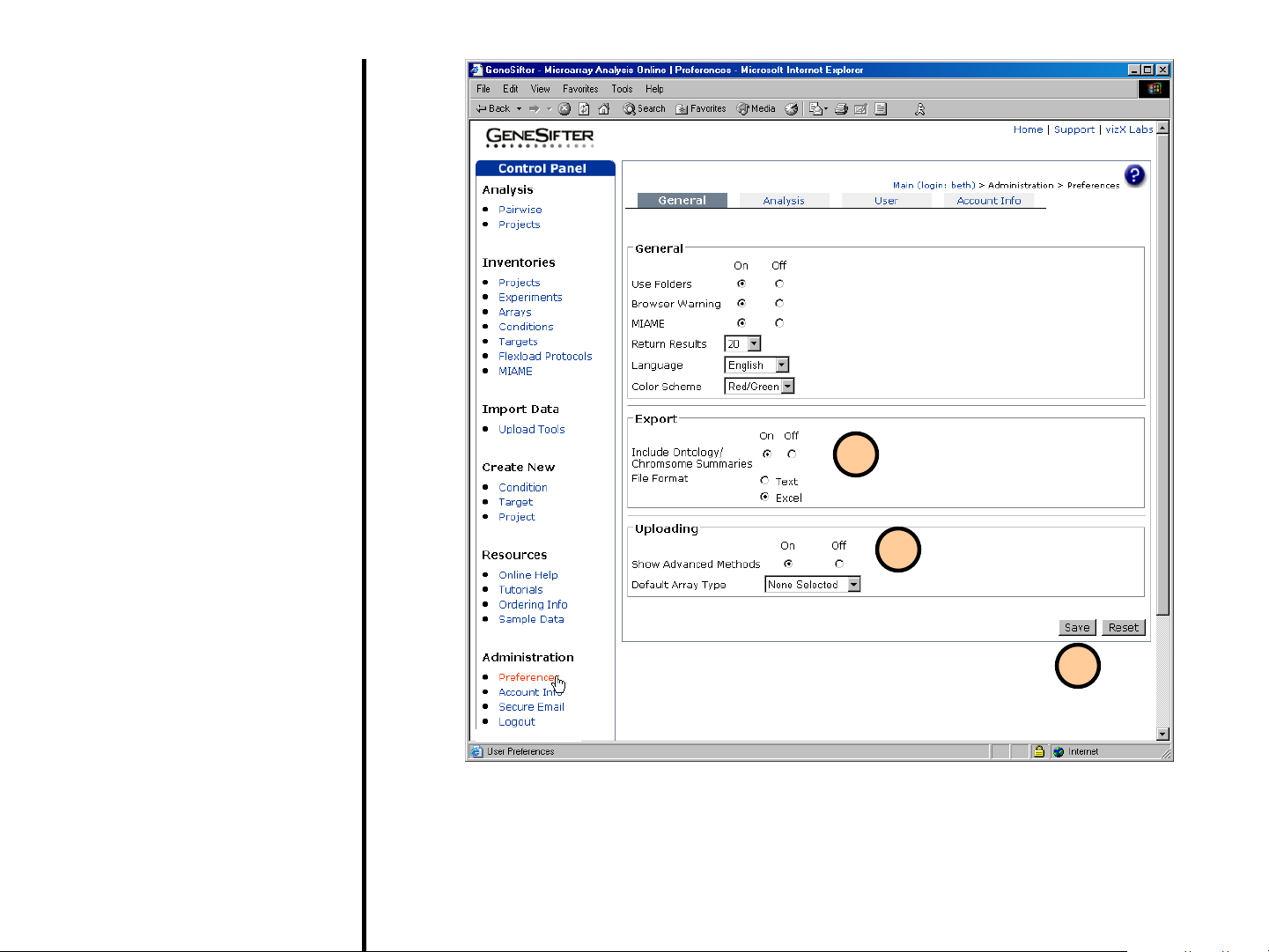
Preferences
1. Select Preferences from the
Control Panel on the left.
Preference options are subdivided
into General, Analysis, User and
Account Info and can be selected
from the tabbed display.
General Preferences
2. General
Use Folders- Toggles the use
of folders in Inventories to help
organize your data.
Browser Warning- Warns
user of unsupported browser.
MIAME- Allows creation and
assignment of MIAME
protocols.
Return Results- Choose
length of the default return for
gene lists.
Language-Select text
language (currently English and
Japanese are available).
Color Scheme- Choose colors
to indicate up and downregulation in displays.
2
1
Page 78
Preferences
(continued)
3. Export
• Include Ontology/
Chromosome SummariesIncludes this information in the
exported file.
• Export Files- Choose whether
exported results are opened
with a text editor or Excel.
4. Uploading
• Show Advanced Methods-
Enables the Advanced Upload
Methods which allows loading
of CEL files, and normalization
with RMA or GC-RMA.
• Default Array Type- Allows
the user to set the Default
Array Type when using the
QuickLoad Wizard.
5. Save desired changes in
Preferences by clicking on the Save
button in the lower right corner.
3
4
5
Page 79

Preferences
Analysis Preferences
4. Advanced Pairwise Settings
4a. When Off is selected, only the basic
parameters for Pairwise Analysis are
available.
4b. When On is selected for Advanced
Pairwise Settings, the pairwise
analysis screen will include these
additional parameters:
• Data Transformation- the ability
to log transform or account for
data already log transformed
• Upper- maximum threshold for
expression
• Correction- The Bonferroni,
Holm, BH and maxT statistical
corrections for multiple testing
4
4a
4b
Page 80

Preferences
Analysis Preferences (continued)
5. Extended Project Data
5a. When Off is selected, only a basic data
summary will be displayed for genes
within Project Analysis
5b. When On is selected, a detailed data
summary will be displayed for selected
genes within the Project Analysis. An
additional table will display all data
points used in the calculation. In
addition to the information in the basic
summary, the detailed summary will
include the following:
• Grp Min - The smallest mean
intensity for that condition
• Grp Max - The largest mean
intensity for that condition
• Grp Ave - The mean of all
intensities within the condition
• Grp Med - The median of all
intensities within the condition
5
5a
5b
Page 81

Preferences
Analysis Preferences (continued)
6. Row Center Project Data displays data
for a selected gene as the intensity for
that gene over the mean intensity for
that gene across all groups.
7. Quality Cutoff defines whether all
groups must pass the selected quality
cutoff or just one of the entire set must
pass.
6
8. Project Gene Title allows the user to
select whether gene titles or accession
numbers are displayed in the project
analysis gene lists.
7
8
Page 82

Preferences
Analysis Preferences (continued)
Heatmap Figure
9 ,9a Heatmap Figure graphically
displays gene regulation in gene
lists. The colors are modulated by
the Color Scheme under General
preferences.
• Number Each Row If the option is
selected, each row of the Heatmap
figure will be consecutively
numbered.
• Open In New Window Upon
clicking “View As Image” in the
project results page, the Heatmap
figure will be opened in a new
browser window.
• Image Type Selects the file format
that the Heatmap image can be
saved as. Available formats are
PNG and JPEG.
9
• Title Upon clicking “View As
Image” in the project results page,
the resulting Heatmap rows can
either be labeled by the gene title or
by the accession number.
10. Gene Titles
Sets the display to either accession
number or the UniGene title within
gene lists. Note that Project Gene
Title under Analysis preferences
will override this selection.
10
9a
Page 83

Preferences
User Preferences
11. User Info
Provides contact information for
sending secure email within
Genesifter.
12. Change Password
To change password, fill in the fields
of old and new password.
13. To save desired changes in
Preferences click on the Save button
in the lower right corner.
11
12
13
Page 84

Preferences
Account Info Preferences
14. Bar graph indicates total account
space used.
14
Page 85

Appendix
GEO Database
Genesifter can upload GEO formatted files
from the Affymetrix platform. The Gene
Expression Omnibus (GEO) is a public
database of microarray data, hosted by the
NCBI (http://www.ncbi.nlm.nih.gov/geo/
1. Query GEO accession
number or the DataSet ID.
2.,3 Alternatively, Browse the
database to find datasets of
interest by selecting
“DataSets”.
4. Select “Geo platform” in the
Sort by pull-down menu to
identify datasets created from
the Affymetrix platform and
thus capable of uploaded into
Genesifter.
)
2
3
1
4
Page 86

GEO Database
(continued)
5. Browse through the datasets
generated using the Affymetrix
platform [Note:GPL91 is the
Affymetrix Platform Accesion
no in GEO]. Select“go to full
dataset record”.
6. To download all the
experiments of the dataset,
mouse over “download” and
select “complete DataSet” and
save the file.
5
6
5
Page 87

GEO Database
(continued)
7. Select Batch Upload option
within Genesifter from the
Control Panel. Enter an
“Array title”, “Description” and
select “This file is a GEO Data
Set” from “Options”.
8. After uploading the GEO file,
Genesifter automatically fills
the Target, Conditions and
Descriptions for each
experiment of the dataset.
These field values can be
changed from Inventories.
Select “Save Data” button to
complete the GEO dataset
import.
7
8
 Loading...