Used Agilent Agilent Used N9342C Manual

Download

Keysight N9342C/43C/44C Handheld Spectrum Analyzer

99 Washington Street Melrose, MA 02176

800.517.8431 TestEquipmentDepot.com

Notice: This document contains references to Agilent. Pl Measurement business has become Keysight Technologies.

ease note that Agilent’s Test and

User's Guide

Notices

any form or by any means (including electronic storage and retrieval or translation into a foreign language) without prior agreement and written consent from Keysight Technologies, Inc. as governed by United States and international copyright laws.

Part Number

N9342-90002

Edition

Fifth Edition, February 2015 Printed in China

Keysight Technologies, Inc. No. 116 Tian Fu 4th Street HiTech Industrial Zone (South) Chengdu 610041, China

Software Revision

This guide is valid for A.03.40 revisions of the N9342C/43C/44C firmware or later.

CAUTION

A CAUTION notice denotes a hazard. It calls attention to an operating procedure, practice, or the like that, if not correctly performed or adhered to, could result in damage to the product or loss of important data. Do not proceed beyond a CAU- TION notice until the indicated conditions are fully understood and met.

WARNING

A WARNING notice denotes a hazard. It calls attention to an operating procedure, practice, or the like that, if not correctly performed or adhered to, could result in personal injury or death. Do not proceed beyond a WARNING notice until the indicated conditions are fully understood and met.

Battery Marking

Keysight Technologies, through Rechargeable Battery Recycling Corporation (RBRC), offers free and convenient battery recycling options in the U.S. and Canada.

Warranty

The material contained in this document is provided “as is,” and is subject to being changed, without notice, in future editions. Further, to the maximum extent permitted by applicable law, Keysight disclaims all warranties, either express or implied, with regard to this manual and any information contained herein, including but not limited to the implied warranties of merchantability and fitness for a particular purpose. Keysight shall not be liable for errors or for incidental or consequential damages in connection with the furnishing, use, or performance of this document or of any information contained herein. Should Keysight and the user have a separate written agreement with warranty terms covering the material in this document that conflict with these terms, the warranty terms in the separate agreement shall control.

Technology Licenses

The hardware and/or software described in this document are furnished under a license and may be used or copied only in accordance with the terms of such license.

Restricted Rights Legend

If software is for use in the performance of a U.S. Government prime contract or subcontract, Software is delivered and licensed as “Commercial computer software” as defined in DFAR 252.227-7014 (June 1995), or as a “commercial item” as defined in FAR

2.101(a) or as “Restricted computer software” as defined in FAR 52.227-19 (June 1987) or any equivalent agency regulation or contract clause. Use, duplication or disclosure of Software is subject to Keysight Technologies’ standard commercial license terms, and non-DOD Departments and Agencies of the U.S. Government will receive no greater than Restricted Rights as defined in FAR

52.227-19(c)(1-2) (June 1987). U.S. Government users will receive no greater than Limited Rights as defined in FAR 52.227-14 (June 1987) or DFAR 252.227-7015 (b)(2) (November 1995), as applicable in any technical data.

1 Overview

Introduction 2

Front Panel Overview 5

Display Annotations 6

Top Panel Overview 8

Instrument Markings 9

2 Getting Started

Checking Shipment and Order List 12

Power Requirements 13

AC Power Cords 14

Safety Considerations 15

Working with Batteries 18

Powering the Analyzer on for the First Time 20

Preparation for Use 21

Power On and Preset Settings 21 Factory Default Settings 22 Visual and Audio Adjustment 23 General System Settings 23 Timed Power On/Off 24 IP configuration 24 Ext Input 24 Show System 25 Adding an Option 26 Show Error 26 Perform Calibration 26 Data Securities 28 Upgrading Firmware 28 Probe Power Output 29

HSA and BSA PC software 30

Making Basic Measurements 31

Contents

3 Functions and Measurements

Measuring Multiple Signals 34

Measuring a Low-Level Signal 39

Improving Frequency Resolution and Accuracy 44

Making Distortion Measurements 45

Making a Stimulus Response Transmission Measurement 51

Measuring Stop Band Attenuation of a Low-pass Filter 53

Making a Reflection Calibration 55

Measuring Return Loss Using the Reflection Calibration Routine 57

Making a Power Measurement with USB Power Sensor 58

Spectrum Monitor 68

Demodulating an FM Signal 70

Modulation Analysis 72

AM/FM Modulation Analysis 72 ASK/FSK Modulation Analysis 75

Channel Scanner 78

Top/Bottom N Channel Scanner 78 List N Channel Scanner 80 Channel Scanner Setup 82

Cable & Antenna Test 83

Preparation 83 Measuring Cable Reflection 84 Measurement Functions 87

File Operation 90

Viewing a file list 90 Saving a file 92 Deleting a file 93 Loading a file 93

4Key Reference

Amptd 96

Display 102

BW 103

RBW 103 VBW 103 VBW/RBW 104 Avg Type 104

Sweep 106

Sweep Time 106 Sweep Type 107 Single Sweep 107 Trigger 108 Gated Sweep 109 Sweep Setup 110

Enter 111

ESC/Bksp 111

Frequency 112

Marker 115

Marker 115 Marker Trace 115 Mode 116 Marker To 118 Function 119 Marker Table 119 Read Out 120 Zoom In/Out 120 Delta Ref 121 All Off 121 Logging Start/Stop 121

Peak 122

MEAS 124

OBW 124 ACPR 125 Channel Power 126 Spectrum Emission Mask (SEM) 128

MODE 135

Spectrum Analyzer 135 Tracking Generator 135 Power Meter 138 Spectrum Monitor 144

SPAN 148

Span 148 Full 148 Zero 148 Last Span 148

Trace 149

Trace 149 Clear Write 149 Max Hold 149 Minimum Hold 150 View 150 Blank 150 Detector 150 Average 152 Average Dura. 152

Limit 153

Limit Type 153 Limit Line 153 Limits 153 Limits Edit 154 Margin 154 Save Limits 154 Recall Limits 154

5Error Messages

Overview 156

Error Message List 157

6 Troubleshooting

Check the basics 162

Contact Keysight Technologies 164

7 Menu Map

Display 167 Sweep 168 FREQ 169 Limit 169 Marker 170 Peak 171 File/Mode - Task Planner 172 Mode - Tracking Generator 173 Mode - Modulation Analysis (AM/FM) 174 Mode - Modulation Analysis (ASK/FSK) 175 Mode - Cable & Antenna Test 176 Mode - Power Meter 177 Meas (1) 178 Meas (2) 179 Span 179 System 180 Trace 181

Overview

1 Overview

The Keysight N934XC is a series of handheld spectrum analyzer with a frequency range from 100 kHz to 20.0 GHz.

N9342C: 100 kHz - 7 GHz

N9343C: 1 MHz - 13.6 GHz

N9344C: 1 MHz - 20 GHz

It provides good usability and exceptional performance for installation and maintenance, spectrum monitoring, and on- site repair tasks. It provides several measurement modes for different applications. Each mode offers a set of automatic measurements that pre- configure the analyzer settings for ease of use.

Overview

Introduction

The analyzer provides ultimate measurement flexibility in a package that is ruggedized for field environments and convenient for mobile applications.

Functionality and Feature

The analyzer provides you with a comprehensive functionality set and measurement convenience, including:

• Power Measurement

provides power measurement functionality on

(Occupied Bandwidth), channel power, and

OBW

(Adjacent Channel Power Ratio).

ACPR

• Spectrum Emission Mask

Provides a Pass/Fail testing capability with a mask for out- of- channel emissions measurement.

• Tracking Generator (Option TG7)

Provides an RF source for scalar network analysis (exclusive for N9342C).

• Spectrum Monitor (Option SIM)

Provides a signal over time. The analyzer can be used to monitor the signal capturing performance or intermittent

• High-sensitivity Measurement (Option PA7, P13, P20)

Includes a pre- amplifier, enabling highly sensitivity measurements, this can be used to measure the low- level signals.

• High Accuracy Power Measurement

Supports Keysight U2000 series (option PWM) and U2020 series (option PWP) power sensors for high accuracy power measurement as a power meter.

the capability to analyze the stability of

event over extended periods of time.

Overview

Introduction

• Baseband Channel (Option BB1)

Provides superior DANL and SSB between 3 kHz to 12 MHz.

• Cable & Antenna Test (Option CA7; Requires option TG7)

Provides a built- in VSWR bridge. Return loss, cable loss and distance- to- fault measurement function are available for the field test.

• Modulation Analysis

Provides AM/FM (option AMA) and ASK/FSK (Option DMA) modulation analysis function.

• Task Planner (Option TPN)

Provides task planner function to integrate different measurements for test automation.

• Time-gated Spectrum Analysis (Option TMG)

Measures any one of several signals separated in time and excludes interfering signals.

• Channel Scanner (Option SCN)

provide the channel scan function in spectrum monitoring, coverage test, and band clearance.

Overview

640 480×

Introduction

Optimized Usability

The analyzer provides the enhanced usability as below:

• The 6.5-inch TFT colorful LCD screen (

enables you to read the scans easily and clearly both

• The arc-shaped handle and rugged rubber casing

ensure a comfortable and firm hold.

• Socket/Telnet remote control via USB, and LAN

port.

• The PC Software on help kit CD provides further

editing and data analysis functions.

• The 3-hour-time battery provides continuous wo

time during field testing.

• The light sensor adjusts the display brightness

according to the environment to save power.

• Keys are back-lit provides easy access in

low- light conditions.

• Keypad can be locked and unlocked with pass-

word to forbid undesired keypad operation.

• Built-in GPS, with built- in GPS antenna (Optio

GPS) offers the GPS location for the field testing.

• User Data Sanitation (Option SEC) allows user to

erase all customized files and data in anal for security.

pixels)

indoors and outdoors.

yzer

Front Panel Overview

N9342CN

Handheld Spectr um Anal yzer

100 kHz - 6.0GHz

Preset

System File Limi t Disp

ABC

2DEF 3

GHI

4JKL 5MNO 6PQR

7STU 8

VWX9YZ_

Mode Meas Trace Amptd

User

Span

Save

Freq

ENTER

Sweep

SHIFT

Peak

Marker

Esc/Bksp

1213

Front Panel Overview

Caption Function

1 Power Switch Toggles the analyzer between on and off

2 Function keys Includes functional hardkeys for measurements.

3 Preset Returns the analyzer to a known state and turns

4 SHIFT Switches alternate upper function of the function

5 Enter Confirms a parameter selection or configuration

6 Peak/Marker Activates the peak search or marker function

7 ESC/Bksp Exits and closes the dialog box or clears the letter

8 Alphanumeric

keys

9 Arrow keys Increases or decreases a parameter step by step

10 Knob Selects the mode or edits a numerical parameter

11 Softkeys Indicates current menu functions on the screen

12 Speaker Actives in demodulation mode

13 Light Sensor Adjusts the screen and hardkey back-light

14 Screen Displays spectrum traces and status information

on/off the power save feature (press for 1 sec.)

keys and Peak/Marker hardkey.

input as a back space key.

includes a positive/negative, a decimal point and ten alphanumeric keys

according to the environmental light.

Overview

Display Annotations

Description Associated Function Key

1 Time and date [System] > {Time/Date}

2 Reference level [Amptd]

3 Amplitude scale [Amptd] > [Scale/Div]

4 Average [Trace] > {More} > {Average}

5 Trace and detector [Trace] > {More} > {Detector}

6 Preamplifier and

sweep and trigger mode

7 Sweep status and

trigger type

8 Center frequency or

start frequency

9 Resolution Bandwidth [BW] > {RBW}

10 Display status line Displays status and messages.

[Amptd] > {Preamp} and [Sweep] > {Trigger}

[Sweep] > {Sweep Setup} and [System] > {Port setting} > {Ext Input}

[Freq]

Display Annotations

Overview

11 Video bandwidth and

frequency offset

12 Frequency span or

stop frequency

13 Sweep time [Sweep] > {Sweep Time}

14 Status annunciator Power and USB stick status

15 Softkey menu See key label description in the Key

16 Softkey menu title Refers to the current activated

17 Remote annunciator

and shift annunciator

18 Marker information [Marker]

19 GPS information [System] > {More} > {GPS}

20 Attenuation [Amplitude] > {Attenuation}

[BW] > {VBW} or [Freq] > {Freq Offset}

[Span] or [Freq] > {Stop Freq}

Reference for more information.

function

Indicates the remote mode and shift key mode

Overview

Ext Pow er

Charging

Ext Trig /

RF Out 50

Antenna

GPS

Probe Power Ext Ref

12-16

VDC

W MAX

RF Input 50

50 VDC MAX 30dBm (1W) M AX

50 VDC MAX

REV PWR

30dBm (1W) MAX

LAN

Top Panel Overview

Items Function

1External DC power

connector

2 LED indicator (Charging) Lights (On) when the battery is charging

3 LED indicator Lights (On) when external DC power is

4 USB interface (Device) Connects to a PC

5 USB interface (Host) Connects to a USB memory stick or disk

6 Headphone Connects to a headphone

7 LAN Interface Connects to a PC for SCPI remote control

8 RF OUT Connector The output for the built-in tracking generator.

9 Probe power connector Provides power for high- impedance AC probes

10 EXT TRIG IN/REF IN

(BNC, Female)

11 GPS antenna connector Connects an GPS Antenna (option GPA) for GPS

12 RF IN Connector (50 Ω) Accepts an external signal input.

Provides input for the DC power source via an AC-DC adapter, or Automotive type DC adapter.

connected.

Enabled with Option TG7.

or other accessories (+15 V, –12 V, 150 mA maximum).

Connects to an external TTL signal or a 10 MHz reference signal. The TTL signal is used to trigger the analyzer’s internal sweep

application.

Instrument Markings

ISM1-A

ICES/NMB-001

The CE mark shows that the product complies with all relevant European Legal Directives.

The CSA mark is a registered trademark of the Canadian Standards Association.

All Level 1, 2 or 3 electrical equipment offered for sale in Australia and New Zealand by Responsible Suppliers must be marked with the Regulatory Compliance Mark.

This symbol is an Industrial Scientific and Medical Group 1 Class A product (CISPR 11, Clause 4)

The ISM device complies with Canadian Interference- Causing Equipment Standard- 001. Cet appareil ISM est conforme à la norme NMB- 001 du Canada.

The instruction manual symbol: indicates that the user must refer to specific instructions in the manual.

The standby symbol is used to mark a position of the instrument power switch.

Indicates the time period during which no hazardous or toxic substance elements are expected to leak or deteriorate during normal use. Forty years is the expected useful life of the product.

Korea Certification indicates this equipment is Class A suitable for professional use and is for use in electromagnetic environments outside of the home.

Instrument Markings

Overview

The symbol indicates this product complies with the WEEE Directive (2002/96/EC) marking requirements and you must not discard this equipment in domestic household waste.

Overview

Instrument Markings

Getting Started

2 Getting Started

Information on checking the analyzer when received, preparation for use, basic instrument use, familiarity with controls, defining preset conditions, updating firmware, and contacting Keysight Technologies.

Getting Started

Checking Shipment and Order List

Check the shipment and order list when you receive the shipment.

• Inspect the shipping container for damages.

Signs of damage may include a dented or torn shipping container or cushioning material that might indicate signs of unusual stress or compacting.

• Carefully remove the contents from the shipping container, and verify if the standard and your ordered options are included in the shipment.

accessories

Power Requirements

Getting Started

Power Requirements

The AC power supplied must meet the following requirements

Voltage : 100 to 240 VAC

Frequency: 50/60 Hz

Power: Maximum 80 W

The AC/DC power supply charger adapter supplied with the analyzer is equipped with a three- wire power cord, in accordance with international safety standards. This power cord grounds the analyzer cabinet when it is connected to an appropriate power line outlet. The power cord appropriate to the original shipping location is included with the analyzer.

Various AC power cables are available from Keysight that are unique to specific geographic areas. You can order additional AC power cords that are appropriate for use in different areas. The AC Power Cord table provides a lists of the available AC power cords, the plug configurations, and identifies the geographic area in which each cable is typically used.

The detachable power cord is the product disconnecting device. It disconnects the main AC circuits from the DC supply. The front- panel switch is only a standby switch and does not disconnect the instrument from the AC LINE power.

Getting Started

250V 10A

125V 10A

230V 15A

250V 16A

AC Power Cords

Plug Type Cable Part

Number

8121-1703 BS 1363/A Option 900

8120-0696 AS 3112:2000 Option 901

250V 10A

8120-1692 IEC 83 C4 Option 902

250V 16A

8120-1521 CNS 10917-2

8120-2296 SEV 1011 Option 906

250V 10A

8120-4600 SABS 164-1 Option 917

8120-4754 JIS C8303 Option 918

125V 15A

8120-5181 SI 32 Option 919

Plug Description

A 5-15P

/NEM

For use in Country & Region

United Kingdom, Hong

ong, Singapore, Malaysia

Australia, New Zealand

Continental Europe, Korea,

nesia, Italy, Russia

Indo

Option 903

Unite States, Canada,

iwan , M e x i co

Switzerland

South Africa, India

Japan

Israel

8120-8377 GB 1002 Option 922

China

250V 10A

a. Plug description describes the p lug only. The part number is for the complete cable assembly.

Safety Considerations

WARNING

Keysight has designed and tested the N934xC handheld spectrum analyzer for measurement, control and laboratory use in accordance with Safety Requirements IEC 61010- 1. The tester is supplied in a safe condition. The N934xC is also designed for use in Installation Category II and Pollution Degree 2 per IEC 61010- 1.

Read the following safety notices carefully before you start to use a N934xC handheld spectrum analyzer to ensure safe operation and to maintain the product in a safe condition.

Personal injury may result if the analyzer’s cover is removed. There are no operator-serviceable parts inside. Always contact Keysight qualified personnel for service. Disconnect the product from all voltage sources while it is being opened.

This product is a Safety Class I analyzer. The main plug should be inserted in a power socket outlet only if provided with a protective earth contact. Any interruption of the protective conductor inside or outside of the product is likely to make the product dangerous. Intentional interruption is prohibited.

Getting Started

Safety Considerations

Electrical shock may result when cleaning the analyzer with the power supply connected. Do not attempt to clean internally.

case only.

Use a dry soft cloth to clean the outside

Always use the three-pin AC power cord supplied with this product. Failure to ensure adequate earth grounding by not using this cord may cause personal injury and product damage.

Getting Started

WARNING

CAU-CAUTION

Safety Considerations

Danger of explosion if the battery is incorrectly replaced. Replace only with the same type battery recommended. Do NOT dispose of batteries in a fire.

Do NOT place batteries in the trash. Batteries must be recycled or disposed of properly.

Recharge the battery only in the analyzer. If left unused, a fully charged battery will discharge itself over time.

Temperature extremes will affect the ability of the battery to charge. Allow the battery to cool down or warm up as necessary before use or charging.

Storing a battery in extreme hot or cold temperatures will reduce the capacity and lifetime of a battery. Battery storage is recommended at a temperature of less than

Never use a damaged or worn-out adapter or battery. Charging the batteries internally, even while the analyzer is powered off, the analyzer may keep warm. To avoid overheating, always disconnect the analyzer from the AC adapter before storing the analyzer into the soft carrying case.

Connect the automotive adapter to the power output connector for IT equipment, when charging the battery on your automotive.

The VxWorks operating system requires full conformity to USB 1.1 or USB 2.0 standards from a USB disk. Not all the USB disk are built that way. If you have problems connecting a particular USB disk, please reboot the analyzer before inserting another USB stick.

The analyzer cannot be used in the standard soft carrying case for more than 1 hours if the ambient temperature is higher than 35

Getting Started

Safety Considerations

Environmental Requirements

The N934xC is designed for use under the following conditions:

• Operating temperature:

C to 40oC (using AC- DC adapter)

C to +50oC (using battery)

–10

• Storage temperature: –40

• Battery temperature: 0

• Humidity: < 95% (40

C to 45oC

C to +70oC

Electrical Requirements

The analyzer allows the use of either a lithium battery pack (internal), AC- DC adapter shipped with the analyzer, or optional automotive +12 VDC adapter for its power supply.

Electrostatic Discharge (ESD) Precautions

This analyzer was constructed in an ESD protected environment. This is because most of the semiconductor devices used in this analyzer are susceptible to damage by static discharge.

Depending on the magnitude of the charge, device substrates can be punctured or destroyed by contact or proximity of a static charge. The result can cause degradation of device performance, early failure, or immediate destruction.

These charges are generated in numerous ways, such as simple contact, separation of materials, and normal motions of persons working with static sensitive devices.

When handling or servicing equipment containing static sensitive devices, adequate precautions must be taken to prevent device damage or destruction. Only those who are thoroughly familiar with industry accepted techniques for handling static sensitive devices should attempt to service circuitry with these devices.

Getting Started

Working with Batteries

The battery provides you approximately 3 hours of operating time for your long time measurement in field test.

Installing a Battery

Step Notes

1 Open the battery cover Use a phillips type screwdriver,

2 Insert the battery Observe correct battery polarity

3 Close the battery cover Push the cover closed, then

loosen the retaining screw, then pull the battery cover open.

orientation when installing.

re-fasten the cover with the retaining screw.

Viewing the Battery Status

Determine the battery status using either of the following methods:

• Check the battery icon in the lower- right corner of the front- panel screen: it indicates the approximate level of charge.

• Press [System] > {System Info} > {Show System} > {Page down} to check the current battery

information.

Getting Started

CAU-CAUTION

Working with Batteries

Charging a Battery

You may charge the battery both in the tester and in the external battery charger (option BCG).

Connect the automotive adapter to the IT power outlet of your automobile (with option 1DC) for battery recharging.

1 Insert the battery in the analyzer.

2 Plug in the AC- DC adapter and switch on the

external power.

3 The charge indicator lights, indicating that the

battery is charging. When the battery is fully charged, the green charging indicator turns off.

During charging and discharging, the battery voltage, current, and temperature are monitored. If any of the monitored conditions exceed their safety limits, the battery will terminate any further charging or discharging until the error condition is corrected.

The charging time for a fully depleted battery, is approximately four hours.

Getting Started

CAU-CAUTION

Install battery

Press Power Switch

Powering the Analyzer on for the First Time

Insert the battery into the analyzer or connect the analyzer to an external power supply via the AC- DC adapter, then press the power switch on the front panel of your N934xC to power on the analyzer.

Use only the original AC-DC adapter or originally supplied battery for the power source.

The maximum RF input level of an average continuous power is 30 dBm (or + connecting a signal into the analyzer that exceeds the maximum level.

Allow the analyzer to warm-up for 30 minutes before making a calibrated measurement. To meet its specifications, the analyzer must meet operating temperature conditions.

50 VDC signal input). Avoid

Preparation for Use

This section provides the basic system configuration which is frequently used before or after the measurement operation.

Power On and Preset Settings

Selecting a preset type

Press [SYS] > {PwrOn/Off Preset} > {Preset Type} to choose the preset types. The analyzer has three types of preset setting for you to choose from:

DFT Restores the analyzer to its factory- defined

settings. The factory default settings can be found, “Factory Default Settings” on page 22.

User Restores the analyzer to a user- defined

setting. Refer to the descriptions as below.

Restores the analyzer to the last setting.

Last

Saving a User-defined Preset

If you frequently use system settings that are not the factory defaults, refer to the following steps to create a user- defined system settings that can be easily recalled:

1 Set the analyzer parameters using the knob, the

arrow keys, or the numeric keypad.

2 Press [SYS] > {PwrOn/Off Preset} > {Save User} to

save the current parameters as the user preset setting.

3 Press [SYS] > {PwrOn/Off Preset} > {Preset Typ e U se r }

to set the preset mode to user defined system setting.

4 Press [Preset]. The instrument will be set to the

state you previously saved.

Getting Started

Preparation for Use

Getting Started

Preparation for Use

Factory Default Settings

Parameter Default Setting

Center Frequency Specific to Product Start Frequency 0.0 Hz Stop Frequency Specific to Product Span Specific to Product Reference Level 0.0 dBm Attenuation Auto (20 dB) Scale/DIV 10 dB/DIV Scale Type Log RBW Auto (3 MHz) VBW Auto (3 MHz) Average Type Log Power Sweep time Auto Sweep Mode Normal Probe Power Off Trace 1 Clear write Trace 2 Blan k Trace 3 Blan k Trace 4 Blan k Trace 1 D e t e c tio n Pos Peak Trace 2 Detection Pos Peak Trace 3 Detection Pos Peak Trace 4 Detection Pos Peak Trace Average All Off Marker All Off Mode Spectrum Analyzer

Getting Started

Preparation for Use

Visual and Audio Adjustment

Display Adjustment

Press [System] > {Brightness} > {Brightness} to toggle the screen brightness between Auto and Man. When it is set to Auto, the brightness adjusts according to the environment automatically with the built-in light sensor. When it is set to Man, you can set a fixed brightness value manually.

Setting Button Backlight

Press [System] > {Keypad Setting} > {BackLight} to tog- gle the backlight button between Auto and Man. You can select the backlight brightness and the auto- off idle time in manual mode.

Setting Key Beep

Press [System] > {Key Settings} >{Beeper} to activate the key beep function as an indicator of key operation.

General System Settings

Provides the following system setting options:

Time/Date

Press [System] > {Time/Date} to set the date and time of the analyzer.

The allowed input for the time is HHMMSS format, and YYYYMMDD format for the date.

Power Saving

Press [System] > {Screen Setting} > {Power Saving} to select a power saving mode which turns off the LCD display after a user- defined idle time. Press any key to re- activate the LCD display after the LCD display power- saving mode has been triggered.

Getting Started

Preparation for Use

Timed Power On/Off

Pressing [System] > {Power On/Off Preset} > {Timed Pwr On} or {Timed Pwr Off} sets the time switch to power

on/off the N934xC in a user- defined time and date. This function requires the power supply to be connected or charged battery installed.

Press {Repeat Mode Once/Everyday} to set the N934xC boot up/off in the pre- saved time everyday. The pre- saved date is invalid in this mode.

IP configuration

The N934xC supports LAN port connection for data transfer. Press [System] > {Port Setting} > {IP Admin} > {IP Address Static} to manually set the IP address, gateway and subnet mask with the proper LAN information. Or, just press [System] > {Setting} > {IP Admin} > {IP Address DCHP} to get the IP address in LAN dynamically according DCHP.

Press {Apply} to enable all the configurations you set.

Ext Input

Toggles the channel for external input between Ref and Tr i g. Ref refers to a 10 MHz reference signal; Tri g refers to a TTL signal.

External Reference (Ref)

Use the external reference function as follows:

1 Input a 10 MHz signal into the EXT TRIG IN/REF IN

connector.

2 Press [System] > {Port Setting} > {Ext Input Ref} to

enable the external reference signal input.

Then, the analyzer will disable the internal reference and switch to accept the external reference.

Getting Started

NOTE

Preparation for Use

External Trigger (Trig)

When an external TTL signal is used for the triggering function, the analyzer uses the inner reference as default.

Use the external trigger function as follows:

1 Press [System] > {Port Setting} > {Ext Input Trig} to

enable the external TTL signal input.

2 Press [SPAN] > {Zero Span} to activate the Tri gg e r

function.

3 Access the associated softkeys to select the

rising edge (Ext Rise) or the falling edge (Ext Fall) as the trigger threshold.

The trace will halt in external trigger mode until the trigger threshold is met or the free run function is activated.

Show System

Pressing [System] > {System Info} > {Show system} displays the following hardware, software, and battery information of the analyzer:

Machine Model Battery Info

MCU Firmware Version Name

DSP Firmware Version Serial NO.

FPGA Firmware Version Capacity

RF Firmware Version Temperature

RF Module S/N Charge Cycles

KeyBoard Module S/N Voltage

This Run Time Current

Temperature Charge Status

Source Voltage Remain Time

Power Source Host ID

Getting Started

Preparation for Use

Adding an Option

Pressing [System] > {More} > {Service} > {Add Option} brings up a dialog box for entering the option license code. Use the numeric keypad to input the option license code and then use the [ENTER] key as a terminator. If the analyzer recognizes the option license code, a message “Option activated successfully” will appear in the status line. Otherwise, a message “Invalid option licence” will appear in the status line. Press [System] > {System

Info} > {Installed Options} to view the options.

Show Error

Pressing [System] > {System Info} > {Error history} accesses a list of the 30 most recent error messages. The most recent error will appear at the bottom of the list. If the error list is longer than 30 entries, the analyzer reports an error message [–350, Query overflow]. For more information, refer to “Error Messages” on page 155.

Perform Calibration

The N934xC provides three manual calibration function to calibrate the time base and amplitude. The analyzer should warm up for 30 minutes before calibration.

Time Base Calibration

Perform a time base calibration to guarantee the frequency accuracy.

When the calibration function is triggered, the current measurement is interrupted and a gauge displays on the LCD. A message will display on the LCD which indicates the calibration is finished, and the interrupted measurement restarts.

Please refer to the operation procedures below:

1 Input a 10 MHz, 0 dBm signal to EXT TRIG IN.

2 Press [System] > {More} > {Service} > {Calibration} >

{Time Base by Ext} to initiate a calibration.

Getting Started

NOTE

Preparation for Use

The analyzer provides the GPS time base calibration function (Option GPS is required). Locate the analyzer on an open ground to receive the GPS signal from satellites. Then press [System]

> {More} > {Service} > {Calibration} > {Time Base by GPS}

to perform a GPS time base calibration.

Time base calibration takes only a short time when the inner temperature is stable. When the inner temperature is increasing, calibration takes a long period of time or will fail. If the input reference signal is abnormal, the calibration cycle will take a long and unpredictable time to exit, and the LCD displays an error message.

Amplitude Calibration

The analyzer provides the internal amplitude calibration function. Please refer to the procedures below to perform an amplitude calibration:

1 Press [System] > {More} > {Service} > {Calibration} >

{Amplitude calibration} > {Calibration}

2 Connect a 50 MHz CW signal to RF IN connector.

The allowed amplitude range is from –2 dBm to 2 dBm. Then press [Enter] to continue.

3 Input the amplitude number of the 50 MHz

signal in the pop- up window and press [Enter] as a terminator.

The analyzer will perform a calibration according to the input amplitude value. Press {Clear data} to set to the factory- preset status with default amplitude calibration data. The amplitude calibration function is only available with the firmware revision A.02.08 or later.

Getting Started

CAU-CAUTION

Preparation for Use

Data Securities

The N934xC offers the optional memory erase function for data security. Press [System] > {More} > {Securities} > {Erase Memory} to erase all the user data in internal memory. Press Enter as a terminator to start the erase process immediately.

The memory erase process takes 15 minutes approximately. During the erase process, there must be a constant power supply to ensure the successful erase. If the erase process is interrupted, please reboot the instrument and erase memory again.

Upgrading Firmware

Please follow the steps below to update the firmware:

1 Download the latest N934xC firmware from

2 Extract files to the root directory of a USB stick.

You will see a folder named “N934xDATA” with file Bappupgrade.hy.

3 Insert the USB stick into the top panel USB

connector.

4 Press [System] > {More} > {Service} > {Upgrade

Firmware} to activate the updating procedure.

Press Enter to upgrade the firmware. The analyzer will perform the update automatically.

5 Unplug the USB stick and restart the analyzer

when message “All modules have been upgraded, please restart” is displayed.

6 Press [System] > {System Info} > {Show System} to

find the updated MCU firmware version.

In updating process, there must be a constant power supply to for at least 15 minutes. If power fails during the updating process it can cause damage to the instrument.

Getting Started

Preparation for Use

Probe Power Output

The Probe Power provides power for high- impedance AC probes or other accessories (+15 V, –12V, 150 mA maximum).

The Probe power is set to off as default. Press [System] > {More} {Port Setting} > {Probe Power On} to switch on the probe power output.

Getting Started

HSA and BSA PC software

Keysight HSA and BSA PC software is an easy- to- use, PC- based remote control tool for the N9342C/43C/44C HSA handheld spectrum analyzer.

It is able to be discretely used as a spectrum monitor to display and control the trace scans simultaneously with the analyzer, or a file manager to send/get files between the analyzer and PC. It also provides some data analysis function for your further use.

For the further description of the HSA PC software, please refer to the online help embedded in this software.

Making Basic Measurements

This section provides information on basic analyzer operations. It assumes that you are familiar with the front and top panel buttons and keys, and display annotations of your analyzer. If you are not, please refer to “Front Panel Overview” on page 5,

“Top Panel Overview” on page 8, and “Instrument Markings” on page 9.

For more details on making measurements, please refer to “Functions and Measurements” on page 33”.

Entering Data

When setting measurement parameters, there are several ways to enter or modify active function values:

1 Using the Front Panel Knob

Increases or decreases the current value.

2 Using the Arrow Keys

Increases or decreases the current value by the step unit defined.

Press [Freq] > {CF Step} to set the frequency by an auto- coupled step (Step = Span/10, when {CF Step} mode is set to Auto).

3 Using the Numeric Keypad

Enters a specific value. Press a terminator key (either a specified unit softkey or [ENTER]) to confirm input.

4 Using the Shift Hardkey

Press the blue shift key first, then press the function hardkeys to select the upper alternative function.

5 Using the Enter Key

Terminates an entry or confirms a selection.

Making Basic Measurements

Getting Started

Making Basic Measurements

Viewing a Signal on the Analyzer

1 Use a signal generator to generate a CW signal

of 1.0 GHz, at a power level of 0.0 dBm.

2 Press [System] > {PwrOn/Off Preset} > {Preset Type}

and select DFT to toggle the preset setting to the factory- defined status.

3 Press the green [Preset] key to restore the

analyzer to its factory- defined setting.

4 Connect the generator’s RF OUT connector to the

analyzer’s RF IN connector.

5 Press [Freq] > 1 > {GHz} to set the analyzer center

frequency to 1 GHz.

6 Press [Span] > 5 > {MHz} to set the analyzer

frequency span to 5 MHz.

7 Press [Peak] to place a marker (M1) at the high-

est peak (1 GHz) on the display.

The Marker amplitude and frequency values appear in the function block and in the upper- right corner of the screen.

Use the front- panel knob, arrow keys, or the softkeys in the Peak Search menu to move the marker and show the value of both frequency and amplitude displayed on the screen.

Figure 2-1 View a signal (1 GHz, 0 dBm)

Functions and Measurements

3 Functions and Measurements

Functions and Measurements

Measuring Multiple Signal s

Measuring Multiple Signals

This section provides information on measuring multiple signals.

Comparing Signals on the Same Screen

The N934xC can easily compare frequency and amplitude signal differences, for example, measuring radio or television signal spectra. The Delta Marker function allows two signals to be compared when both appear on the screen at the same time.

In the following example, a 50 MHz signal is used to measure frequency and amplitude differences between two signals on the same screen. The Delta Marker function is demonstrated in this example.

1 Press [Preset] to set the analyzer to the factory

default setting.

2 Input a signal (0 dB, 50 MHz) to the RF IN

connector of the analyzer.

3 Set the analyzer start frequency, stop frequency,

and reference level to view the 50 MHz signal and its harmonics up to 100 MHz:

• Press [FREQ] > 40 > {MHz}

• Press [FREQ] > 110 > {MHz}

• Press [AMPTD] > 0 > {dBm}

4 Press [PEAK] to place a marker on the highest

peak on the display (50 MHz).

The {Next Left PK} and {Next Right PK} softkeys are available to move the marker from peak to peak.

5 Press [Marker] > {Delta} to anchor the first marker

(labeled as M1) and activate a delta marker.

The label on the first marker now reads 1R, indicating that it is the reference point.

Functions and Measurements

NOTE

Measuring Multiple Signals

6 Move the second marker to another signal peak

using the front panel knob. In this example the next peak is 100 MHz, a harmonic of the 50 MHz signal:

Press [Peak] > {Next Right PK} or {Next Left PK}.

To increase the resolution of the marker readings, turn on the frequency count function. For more information, please refer to

“Improving Frequency Resolution and

Accuracy” on page 44

Figure 3 Del ta pair marker with signals (same screen)

Functions and Measurements

Frequency

Enter

MOD On/Off

102

On/Off

Amplitude FM

Utility

LF Out

Preset

Local

AM I/Q

File

Trigger

PulseM

Sweep

Remote

Standby

N9310A RF Signal Generator 9 kHz - 3.0 GHz

REVERSE PWR 4W MAX 30VDC

LF OUT RF OUT 50

FUNCTIONS

Frequency

Enter

MOD On/Off

102

On/Off

Amplitude FM

Utility

LF Out

Preset

Local

AM I/Q

File

TriggerPulseM

Sweep

Remote

Standby On

N9310A RF Signal Generator 9 kHz - 3.0 GHz

REVERSE PWR 4W MAX 30VDC

LF OUT RF OUT 50

FUNCTIONS

Directional coupler

Signal generator

Measuring Multiple Signal s

Resolving Signals of Equal Amplitude

In this example a decrease in resolution bandwidth is used in combination with a decrease in video bandwidth to resolve two signals of equal amplitude with a frequency separation of 100 kHz.

Notice that the final RBW selected is the same width as the signal separation, while the VBW is slightly narrower than the RBW.

1 Connect two sources to the analyzer input as

shown below.

Figure 4 Setup for obtaining two signals

2 Set on

e source to 300 MHz. Set the frequency of the other source to 300.1 MHz. Set both source amplitudes to –20 dBm.

3 Setup the analyzer to view the signals:

• Press [PRESET]

• Press [FREQ] > 300.05 > {MHz}

• Press [SPAN] > 2 > {MHz}

• Press [BW] > 30 > {kHz}

Functions and Measurements

Measuring Multiple Signals

Use the knob or the arrow keys to further reduce the resolution bandwidth and better resolve the signals.

As you decrease the resolution bandwidth, you improve the resolution of the individual signals and it also increases the sweep timing. For fastest measurement times, use the widest possible resolution bandwidth.

Under factory preset conditions, the resolution bandwidth is coupled to the span.

Figure 5 Resol ving signals of equal amplitude

Functions and Measurements

Measuring Multiple Signal s

Resolving Small Signals Hidden by Large

Signals

This example uses narrow resolution bandwidths to resolve two input signals with a frequency separation of 50 kHz and an amplitude difference

of 60 dB.

1 Connect two sources to the analyzer input

connector as shown in Figure 4 on page 36.

2 Set one source to 300 MHz at –10 dBm. Set the

other source to 300.05 MHz at –70 dBm.

3 Set the analyzer as follows:

• Press [PRESET]

• Press [FREQ] > 300.05 > {MHz}

• Press [SPAN] > 500 > {kHz}

• Press [BW] > 300 > {Hz}

4 Reduce the resolution bandwidth filter to view

the smaller hidden signal. Place a delta marker on the smaller signal:

• Press [Peak]

• Press [MARKER] > {Delta}

• Press [Peak] > {Next Right PK} or {Next Left PK}

Figure 6 Resol ving a small signal hidden by a larger signal

Functions and Measurements

Measuring a Low-Level Signal

This section provides information on measuring low- level signals and distinguishing them from spectrum noise. There are four techniques used to measure low- level signals.

Reducing Input Attenuation

The ability to measure a low- level signal is limited by internally generated noise in the spectrum analyzer.

The input attenuator affects the level of a signal passing through the analyzer. If a signal is very close to the noise floor, reducing input attenuation will bring the signal out of the noise.

1 Preset the analyzer:

2 Input a signal (1 GHz, –80 dBm) to RF IN.

3 Set the CF, span and reference level:

• Press [FREQ] > 1 > {GHz}

• Press [SPAN] > 5 > {MHz}

• Press [AMPTD] > –40 > {dBm}

4 Move the desired peak (1 GHz) to the center of

the display:

• Press [Peak]

• Press [MARKER] > {Marker To} > {To Center}

Figure 7 A signal closer to the noise level (Atten: 10 dB)

Functions and Measurements

Measuring a Low-Level Signal

5 Reduce the span to 1 MHz and if necessary

re- center the peak.

• Press [SPAN] > 1 > {MHz}

6 Set the attenuation to 20 dB. Note that increas-

ing the attenuation moves the noise floor closer to the signal level.

• Press [AMPTD] > {Attenuation} > 20 > {dB}

Figure 8 A signal closer to the noise level (Atten: 20 dB)

7 Press [AMPTD] >

attenuation to 0 dB.

Figure 9 A signal closer to the noise level (Atten: 0 dB)

{Attenuation} > 0 > {dB} to set the

Functions and Measurements

Measuring a Low-Level Signal

Decreasing the Resolution Bandwidth

Resolution bandwidth settings affect the level of internal noise without affecting the amplitude level of continuous wave (CW) signals. Decreasing the RBW by a decade reduces the noise floor by 10 dB.

1 Refer to “Reducing Input Attenuation” on page 39,

and follow steps 1, 2 and 3.

2 Decrease the resolution bandwidth:

• Press [BW], and toggle RBW setting to Man

(manual), then decrease the resolution bandwidth using the knob, the arrow keys or the numeric keypad.

The low level signal appears more clearly because the noise level is reduced.

Figure 10 Decreasing resolution band width

Functions and Measurements

Measuring a Low-Level Signal

Using the Average Detector and

Increased Sweep Time

The analyzer’s noise floor response may mask low- level signals. Selecting the instruments averaging detector and increasing the sweep time will smooth the noise and improve the signal’s visibility. Slower sweep times are necessary to average noise variations.

1 Refer to “Reducing Input Attenuation” on page 39,

and follow steps 1, 2, and 3.

2 Press [TRACE] > {More} > {Detector} > {Average} to

select the average detector.

3 Press [Sweep] > {Sweep Time} to set the sweep

time to 500 ms. Note how the noise appears to smooth out. The analyzer has more time to average the values for each of the displayed data points.

4 Press [BW] > {Avg Type} to change the average

type.

Figure 11 Using the average detector

Functions and Measurements

NOTE

Measuring a Low-Level Signal

Tra ce Av era gin g

Averaging is a digital process in which each trace point is averaged with the previous sweep’s data average for the same trace point.

Selecting averaging, when the analyzer is auto coupled, changes the detection mode to sample, smoothing the displayed noise level.

This is a trace processing function and is not the same as using the average detector (as described on

1 Refer to the first procedure “Reducing Input

Attenuation” on page 39, and follow steps 1, 2,

and 3.

2 Press [TRACE] > {Average} (On) to turn average on.

3 Press 50 > [ENTER] to set the average number to

50.

As the averaging routine smooths the trace, low level signals become more visible.

Figure 12 Trace averaging

page 42).

Functions and Measurements

NOTE

Improving Frequency Resolution and Accuracy

This section provides information on using the frequency counter to improve frequency resolution and accuracy.

Marker count properly functions only on CW signals or discrete spectral components. The marker must be > 40 dB above the displayed noise level.

1 Press [PRESET] (factory preset)

2 Input a signal (1 GHz, –30 dBm) to the ana-

lyzer’s RF IN connector.

3 Set the center frequency to 1 GHz and the span

MHz.

to 5

4 Press [MARKER] > {Function} > {Counter} to turn the

frequency counter on.

5 Move the marker by rotating the knob to a point

half- way down the skirt of the signal response.

6 Press [MARKER] > {Function} > {Normal} to turn off

the marker counter.

Figure 13 Using the frequency counter

Functions and Measurements

Making Distortion Measurements

This section provides information on measuring and identifying signal distortion.

Identifying Analyzer Generated Distortion

High level input signals may cause analyzer distortion products that could mask the real distortion present on the measured signal. Use trace and the RF attenuator to determine which signals, if any, may be internally generated distortion products.

In this example, a signal from a signal generator is used to determine whether the harmonic distortion products are generated by the analyzer.

1 Input a signal (200 MHz, –10 dBm) to the

analyzer RF IN connector.

2 Set the analyzer center frequency and span:

• Press [Preset] (factory preset)

• Press [Freq] > 400 > {MHz}

• Press [Span] > 700 > {MHz}

The signal produces harmonic distortion products

200 MHz from the original 200 MHz signal).

(spaced

Figure 14 Harmonic d istortion

Functions and Measurements

Making Distortion Measurements

3 Change the center frequency to the value of the

second (400 MHz) harmonic:

• Press [Peak]

• Press [Marker] > {Marker To} > {To Center}

4 Change the span to 50 MHz and re- center the

signal:

• Press [Span] > 50 > {MHz}

• Press [Peak]

5 Set the attenuation to 0 dB:

• Press [Amptd] > {Attenuation} > 0 > {dB}

• Press [Marker] > {Marker To} > {To Ref}

6 To determine whether the harmonic distortion

products are generated by the analyzer, first save the trace data in trace 2 as follows:

• Press [Trace] > {Trace (2)}

• Press [Trace] > {Clear Write}

7 Allow trace 2 to update (minimum two sweeps),

then store the data from trace 2 and place a delta marker on the harmonic of trace 2:

• Press [Trace] > {View}

• Press [Peak]

• Press [Marker] > {Delta}

The Figure 15 shows the stored data in trace 2 and the measured data in trace 1. The Marker Delta indicator reads the difference in amplitude between the reference and active trace markers.

Functions and Measurements

Making Distortion Measurements

Figure 15 Identifying Analyzer Distortion (O dB atten)

ess [AMPTD] > {Attenuation} > 10 > {dB} to

8 Pr

increase the RF attenuation to 10 dB.

Figure 16 Identifying Analyzer Distortion (10 dB atten)

The marker readout comes from two sources:

eased input attenuation causes poorer

• Incr

signal- to- noise ratio. This causes the marker delta value to be positive.

• Reduced contribution of the analyzer circuits

to the harmonic measurement causes the marker to be negative.

A large marker delta value readout indicates significant measurement errors. Set the input attenuator at a level to minimize the absolute value of marker delta.

Functions and Measurements

Frequency

Enter

MOD On/Off

102

On/Off

Amplitude FM

Utility

LF Out

Preset

Local

AM I/Q

File

TriggerPulseM

Sweep

Remote

Standby On

N9310A RF Signal Generator 9 kHz - 3.0 GHz

REVERSE PWR 4W MAX 30VDC

LF OUT RF OUT 50

FUNCTIONS

Frequency

Enter

MOD On/Off

102

On/Off

Amplitude FM

Utility

LF Out

Preset

Local

AM I / Q

File

TriggerPulseM

Sweep

Remote

Standby

N9310A RF Signal Generator 9 kHz - 3.0 GHz

REVERSE PWR 4W MAX 30VDC

LF OUT RF OUT 50

FUNCTIONS

Signal generator

Directional coupler

Making Distortion Measurements

Third-Order Intermodulation Distortion

Two- tone, third- order intermodulation (TOI) distortion is a common test in communication systems. When two signals are present in a non- linear system, they may interact and create third- order intermodulation distortion products that are located close to the original signals. System components such as amplifiers and mixers generate these distortion products.

In this example we test a device for third-order intermodulation using markers. Two sources are used, one is set to 300 MHz and the other to 301 MHz.

1 Connect the equipment as shown in figure below.

This combination of signal generators and directional coupler (used as a combiner) results in a two- tone source with very low intermodulation distortion.

Although the distortion from this setup may be better than the specified performance of the analyzer, it is useful for determining the TOI performance of the source/analyzer combination.

Functions and Measurements

NOTE

Making Distortion Measurements

After the performance of the source/analyzer combination has been verified, the DUT (device under test, for example, an amplifier) would be inserted between the directional coupler output and the analyzer input.

The coupler used should have a high isolation between the two input ports to limit the sources intermodulation.

2 Set one source (signal generator) to 300 MHz

and the other source to 301 MHz. This will define the frequency separation at 1 MHz. Set both sources equal in amplitude, as measured by the analyzer. In this example, they are both set to –5 dBm.

3 Set the analyzer center frequency and span:

• Press [PRESET] (Factory preset)

• Press [FREQ] > 300.5 > {MHz}

• Press [SPAN] > 5 > {MHz}

4 Reduce the RBW until the distortion products

are visible:

• Press [BW] > {RBW}, and reduce the RBW using

the knob, the arrow keys or the numeric keypad.

5 Move the signal to the reference level:

• Press [Peak]

• Press [MARKER] > {Marker To} > {To Ref}

6 Reduce the RBW until the distortion products

are visible:

• Press [BW] > {RBW}, and reduce the RBW using

the knob, the arrow keys or the numeric keypad.

7 Activate the second marker and place it on the

peak of the distortion product (beside the test signal) using the Next Peak:

• Press [MARKER] > {Delta}

• Press [Peak] > {Next Left (Right) PK}

Functions and Measurements

Making Distortion Measurements

8 Measure the other distortion product:

• Press [MARKER] > {Normal}

• Press [Peak] > {Next Left (Right) Peak}

9 Measure the difference between this test signal

and the second distortion product.

• Press [MARKER] > {Normal}

• Press [Peak] > {Next Left/Right Peak}

Figure 17 TOI test screen

Making a Stimulus Response Transmission Measurement

N9340A

HANDHELD SPECTRUM ANALYZER

100 kHz - 3.0 GHz

PRESET

ENTER

FREQ SPANAMPTD

BW/ SWP

SYS MO DE MEAS TRACE

ESC/CLR

2DEF 3GHI1ABC

5MNO4JKL

PQR

VWX7STU9YZ_

0SAVE

LIMIT

MARKER

DUT

CAU-CAUTION

Functions and Measurements

Making a Stimulus Response Transmission Measurement

The procedure below describes how to use a built-in tracking generator to measure the rejection of a low pass filter, a type of transmission measurement.

1 To measure the rejection of a low pass filter,

connect the equipment as shown below. A 370 MHz low- pass filter is used as a DUT in this example.

Figure 18 Transmission Measurement Test Setup

2 Press [Pres

et] to perform a factory preset.

3 Set the start and stop frequencies and resolution

bandwidth:

• Press [FREQ] > {Start Freq} > 100 > {MHz}

• Press [FREQ] > {Stop Freq} > 1 > {GHz}

• Press [BW] > {RBW} > 1 > {MHz}

4 Turn on the tracking generator and if necessary,

set the output power to –10 dBm:

Press [MODE] > {Track Generator} > {Amplitude (On)} >

–10 > {dBm}.

Excessive signal input may damage the DUT. Do not exceed the maximum power that the device under test can tolerate.

Functions and Measurements

Making a Stimulus Response Transmission Measurement

5 Press [Sweep] > {Sweep Time (Auto)} to put the

sweep time into stimulus response auto coupled mode.

6 Increase the measurement sensitivity and smooth

the noise:

Press [BW] > {RBW} > 30 > {kHz} Press [BW] > {VBW} > 30 > {kHz}

A decrease in the displayed amplitude is caused by tracking error.

7 Connect the cable from the tracking generator

output to the analyzer input. Store the frequency response in trace 4 and normalize:

Press [MEAS] > {Normalize} > {Store Ref} (1 → 4) >

{Normalize (On)}

8 Reconnect the DUT to the analyzer and change

the normalized reference position:

Press [MEAS] > {Normalize} > {Norm Ref Posn} > 8 >

[ENTER]

9 Measure the rejection of the low- pass filter:

Press [Marker] > {Normal} > 370 > MHz, {Delta} > 130

> {MHz}

The marker readout displays the rejection of the filter at 130 MHz above the cutoff frequency of the low- pass filter.

Figure 19 Measure the Rejection Range

Measuring Stop Band Attenuation of a Low-pass Filter

CAU-CAUTION

Functions and Measurements

Measuring Stop Band Attenuation of a Low-pass Filter

When measuring filter characteristics, it is useful to look at the stimulus response over a wide frequency range. Setting the analyzer x- axis (frequency) to display logarithmically provides this function. The following example uses the tracking generator to measure the stop band attenuation of a 370 MHz low pass filter.

1 Connect the DUT as shown in Figure 18 on

page 51. This example uses a 370 MHz low pass

filter.

2 Press [Preset] to perform a factory preset.

3 Set the start and stop frequencies:

• Press [FREQ] > {Start Freq} > 100 > {MHz}

• Press [FREQ] > {Stop Freq} > 1 > {GHz}

• Press [AMPTD] > {Scale Type} > {Log}

4 Press [BW] > 10 > {kHz} to set the resolution

bandwidth to 10 kHz.

Excessive signal input may damage the DUT. Do not exceed the maximum power that the device under test can tolerate.

5 Turn on the tracking generator and if necessary,

set the output power to - 10 dBm:

Press [MODE] > {Track Generator} > {Amplitude (On)} >

–10 > {dBm}.

6 Press [Sweep] > {Sweep Time (Auto)} to put the

sweep time into stimulus response auto coupled mode. Adjust the reference level if necessary to place the signal on screen.

7 Connect the cable (but not the DUT) from the

tracking generator output to the analyzer input. Store the frequency response into trace 4 and normalize:

Press [MEAS] > {Normalize} > {Store Ref} (1 → 4) >

{Normalize (On)}

Functions and Measurements

Measuring Stop Band Attenuation of a Low-pass Filter

8 Reconnect the DUT to the analyzer. Note that the

units of the reference level have changed to dB, indicating that this is now a relative measurement.

9 To change the normalized reference position:

Press [MEAS] > {Normalize} > {Norm Ref Posn} > 8 >

[ENTER]

10Place the reference marker at the specified cut-

off frequency: Press [MARKER] > {Mode} > {Normal} > 370 > MHz

11 Set the 2nd marker as a delta frequency of

MHz:

Press {Delta} > 37 > MHz

12In this example, the attenuation over this

frequency range is 19.16 dB/octave (one octave above the cutoff frequency).

13Use the front- panel knob to place the marker at

the highest peak in the stop band to determine the minimum stop band attenuation. In this example, the peak occurs at 600 MHz. The attenuation is 51.94 dB.

Figure 20 Minimum Stop Band Attenuation

Functions and Measurements

N9340A

HANDHELD SPECTRUM ANALYZER

100 kHz - 3.0 GHz

PRESET

ENTER

FREQ SPANAMPTD

BW/ SWP

SYS MODE MEAS TRACE

ESC/CLR

2DEF 3GHI1ABC

5MNO4JKL

PQR

8VWX7ST U 9 YZ_

0SAVE

LIMIT

MARKER

Coupled Port

Short

Circuit

DUT

NOTE

Making a Reflection Calibration

The following procedure makes a reflection calibration using a coupler or directional bridge to measure the return loss of a filter. This example uses a 370 MHz low- pass filter as the DUT. The tracking generator (option TG7) is needed for this measurement. For N9342C handheld spectrum analyzer with option CA7 or CAU, please refer to the “Measuring Cable Reflection” on page 84 to make a reflection measurement.

The calibration standard for reflection calibration is usually a short circuit connected at the reference plane (the point at which the DUT is connected). A short circuit has a reflection coefficient of 1 (0 dB return loss). It reflects all incident power and provides a convenient 0 dB reference.

1 Connect the DUT to the directional bridge or

coupler as shown below. Terminate the unconnected port of the DUT.

Figure 21

Reflection Measurement Short Calibration Test Setup

If possible, use a coupler or bridge with the correct test port connector types for both calibrating and measuring. For the best results, use the same adapter for the calibration and the measurement. Terminate the second port of a two port device.

2 Connect the tracking generator output of the

analyzer to the directional bridge or coupler.

Functions and Measurements

CAU-CAUTION

NOTE

Making a Reflection Calibration

3 Connect the analyzer input to the coupled port

of the directional bridge or coupler.

4 Press [Preset] to perform a factory preset.

5 Turn on the tracking generator and if necessary,

set the output power to –10 dBm:

Press [MODE] > {Track Generator} > {Amplitude (On)} >

–10 > {dBm}

Excessive signal input may damage the DUT. Do not exceed the maximum power that the device under test can tolerate.

6 Set the start and stop frequencies and RBW:

• Press [FREQ] > {Start Freq} > 100 > {MHz}

• Press [FREQ] > {Stop Freq} > 1 > {GHz}

• Press [BW] > 1 > MHz

7 Replace the DUT with a short circuit. 8 Press [MEAS] > {Normalize} > {Store Ref (1 → 4)} >

{Normalize (On)} to normalize the trace.

It activates the trace 1 minus trace 4 function and displays the results in trace 1. The normalized trace or flat line represents 0 dB return loss. Normalization occurs in each sweep. Replace the short (cal device) with the DUT.

Since the reference trace is stored in trace 4, changing trace 4 to Clear Write invalidates the normalization.

Figure 22 Short Circuit Normalized

Measuring Return Loss Using the Reflection Calibration Routine

Functions and Measurements

Measuring Return Loss Using the Reflection Calibration Routine

This procedure uses the reflection calibration routine in the previous procedure “Making a

Reflection Calibration” on page 55, to calculate the

return loss of the 370 MHz low- pass filter.

1 After calibrating the system with the above

procedure, reconnect the filter in place of the short (cal device) without changing any analyzer settings.

2 Use the marker to read return loss. Position the

marker with the front-panel knob to read the return loss at that frequency.

Rotate the knob to find the highest peak and the readout is the maximum return loss.

Figure 23 Measuring the Return Loss of the Filter

Functions and Measurements

CAU-CAUTION

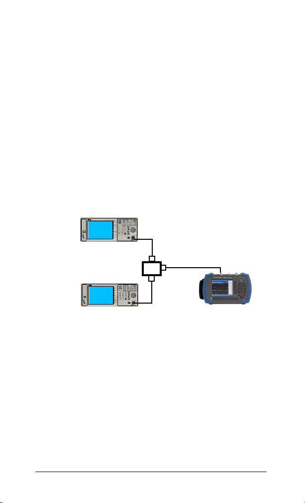
Making a Power Measurement with USB Power Sensor

Average power measurements provide a key metric in transmitter performance.

Base station transmit power must be set accurately to achieve optimal coverage in wireless networks. If the transmit power is set too high due to inaccurate power measurements, undesired interference can occur. If the transmit power is set too low, coverage gaps or holes may occur. Either case may affect system capacity and may translate into decreased revenue for service providers.

Figure 24 Connection with base station

Average power can be measured for the channel of

erest while the base station is active. All other

int channels should be inactive. Average power is a broadband measurement. If other signals are present the analyzer will also measure their power contributions.

The maximum power for the RF IN port and the RF OUT port of the analyzer is +20 dBm. The maximum power for the Power Sensor port is +24 dBm. When directly coupled to a base station, the test set can be damaged by excessive power applied to any of these three ports.

To prevent damage in most situations when directly coupling an analyzer to a base station, use a high power attenuator between the analyzer and the BTS.

Making a Power Measurement with USB Power Sensor

NOTE

Functions and Measurements

The N934xC spectrum analyzer supports the U2000 and U2020 series USB power sensors.

The U2000 Series USB power sensors do not need manual calibration and zero routines performed. Calibration and zeroing are performed without removing the power sensor from the source, through internal zeroing. With internal zeroing of U2000 Series USB power sensors, there is no need to disconnect the sensor or power- off the DUT. The U2000 Series do not require 50 MHz reference signal calibration, allowing the factory calibration to ensure measurement accuracy. For best accuracy, users are recommended to perform external zeroing for input signals below - 30 dBm for best accuracy

If you suspect other signals may be present, it is recommended that you turn off all the other channels and

measure average power only on the signal of interest. Another option is to measure channel power (which is less

accurate), that filters out all other channels (signals). You can measure channel power for CDMA using the CDMA Analyzer or CDMA Over Air tool. For other modulation formats, use their respective analyzers (that is, GSM, 1xEV-DO, or W-CDMA) or measure channel power using either the spectrum analyzer or the Channel Scanner tool.

Connect the power meter as close as possible to the power amplifier/duplexer output. Do not use a coupled port. Sensors may not be as accurate at the power levels provided by coupled ports.

Functions and Measurements

CAU-CAUTION

Making a Power Measurement with USB Power Sensor

Making an Average Power Measurement

To make an average power measurement, connect the power sensor and cable, zero and calibrate the meter, before making a measurement.

Zeroing of the Power Meter will occur automatically:

• Every time the Power Meter function is used.

• When a 5 degree C. change in instrument

temperature occurs.

• Whenever the power sensor is changed.

• Every 24 hours (min.).

• Before measuring low level signals -for example,

10 dB above the lowest specified power the power sensor is capable of.

Calibrate the Power Meter every time you cycle the power on and off.

In most situations, you can press {Zero} to complete the two steps (zero and cal) together.

To Make a Basic Average Power Measurement

You can follow the steps below to make a basic average power measurement.

1 Press [Preset] to perform a factory preset.

2 Press [MODE] > {Power Meter} to access the power

meter mode.

3 Zero and calibrate the meter. Press {Zeroing} to

make a zero operation of the power sensor followed by a calibration operation.

4 Connect the power sensor to the RF Input

50 MHz port. The analyzer supports the U2000 series power sensors.

To prevent damage to your sensor, do not exceed the power levels below. U2000/1/2A +25 dBm (320 mW) average, 20 VDC

+33 dBm (2 W) peak, <10 μs For more information on the maximum power of U2000 series

power sensors, please refer to the Operating and Service Guide of Keysight U2000 Series USB Power Sensors.

Making a Power Measurement with USB Power Sensor

5 Connect the external attenuation, if required,

with the power sensor used.

6 Connect the power sensor to the signal to be

measured. A typical base transceiver station connection is after the output of the power amplifier and duplexer. The connection requires a 2 ft. cable and two Type- N barrel connectors, in addition to the power sensor and external attenuator.

7 Press Meas Setup > Disp Range to set the display

range of the measurement. when it is set to On, the display range will be adjusted automatically according to the signal power dynamic range. When it is set to Off, press To p and Bottom to set the display range manually.

8 Press General Setup > Freq to set the power fre-

quency for the DUT. The current frequency will display in the bottom line.

9 Press Power Range > Auto Power to toggles the

measurement range between On and Off. When it is set to On, the power range will be adjusted automatically. Use auto range when you are not sure of the power level you are about to measure. When it is set to Off, press Range to select the upper range or lower range. The lower range uses the more sensitive path and the upper range uses the attenuated path.

Table 1 Power Sensor Range

Functions and Measurements

Sensor Lower range Upper range

U2000/1/2/4A –60 dBm to –7 dBm –7 dBm to +20 dBm

U2000/1/2H –50 dBm to +3 dBm +3 dBm to +30 dBm

U2000/1B –30 dBm to +23 dBm +23 dBm to +44 dBm

Functions and Measurements

Making a Power Measurement with USB Power Sensor

10Press Meas > Meas Seup > Disp Mode to set the

display in meter. chart or trace display. the measurement result will displays on the screen as shown.

Figure 25 Power Measurement

Making a Power Measurement with USB Power Sensor

NOTE

Functions and Measurements

Making a Peak Power Measurement

The Keysight U2020 X-series USB peak and average power sensors enable peak power measurements that have the same accuracy as measurements obtained using traditional peak power meters, while providing the advantages of being a very compact and portable form factor.

Follow the steps below to make a peak power measurement.

1 Press Mode > Power Meter to access the power

meter mode.

2 Connect the power sensor to the USB port of

N9322C. The sensor will automatically initialize, perform zeroing (While remaining connected to the device under test), and calibrate without connecting to an external source.

You can manually perform zeroing and calibration by pressing Zeroing > Zeroing and Calibration at any time after the sensor is connected and initialized.

3 Press General Setup > Freq to set the frequency of

the signal under test.

As a wideband device, the power sensor has a frequency response. The power sensor utilizes a complex correction algorithm to remove power measurement error due to linearity error, frequency response, and temperature drift to generate a more accurate measurement.

The analyzer provide the customer preset function with U2020 X- series power sensor. Press Meas > Preset and the predefined protocol list will pop up. Select the wanted item and press Preset as a terminator. The related settings will be set automatically.

Functions and Measurements

Making a Power Measurement with USB Power Sensor

Figure 26 Customized Preset the U2020 Power Sensor

Marker Readings

4 Press Mea

measurement results as Figure 27 below.

Figure 27 Peak Power Measurement

s Disp > Disp Mode > Trace to find the

Gate Results

Pulse Parameter Results

Making a Power Measurement with USB Power Sensor

Functions and Measurements

Power Meter Settings

Please find the sections below to find the general power meter measurement settings.

Setting Power Meter Resolution

You can choose from four levels of Power Meter resolution. Higher resolutions provide more accuracy but slow the measurement speed.

1 Press [Preset] to perform a factory preset.

2 Press [MODE] > {Power Meter} to access the power

meter mode.

3 Press {Meas Disp} > {Resolution}. Select 1,2,3 or 4.

The four options represent different resolution as follow:

• [1] = 1

• [2] = 0.1

• [3] = 0.01

• [4] = 0.001

Setting the Power Meter’s Top and Bottom End-Points

Setting the end points (Disk Range) close to the expected measurement value changes the sensitivity of the Power Meter scale resolution. This is an advantage in viewing small changes in power. However, this will not affect the overall range of the sensor.

1 Press [Preset] to perform a factory preset.

2 Press [MODE] > {Power Meter} to access the power

meter mode.

3 Press {Meas Disp} > {Disp Range} to access the

end- points menu.

4 Press {Top} and enter the maximum scale value

desired using the numeric keypad. Then press {dBm} to complete the setup.

5 Press {Bottom} and enter the minimum scale value

desired using the numeric keypad. Then press {dBm} to complete the setup.

Functions and Measurements

Making a Power Measurement with USB Power Sensor

Setting the Power Meter’s Upper and Lower Limits

The internal Power Meter can be configured to detect when a measurement has failed a user predefined upper and lower limits.

1 Press [Preset] to perform a factory preset.

2 Press [MODE] > {Power Meter} to access the power

meter mode.

3 Press {Meas Setup} > {Limits} to access the limits

menu.

4 Press {Limits} to activate the limits function. Each

time the softkey is pressed, the selected option changes.

5 Press {Upper Limits} and enter the high limit value

using the numeric keypad. Then press {dBm} to complete the setup.

Press {Lower Limits} and enter the low limit value using the numeric keypad. Then press {dBm} to complete the setup.

Set the Step Detection

Press Meas > General Setup > Average > Step Detect to set the step Detect On and Off. When it is set to on, the filter will re- initialize upon detection of a step increase or decrease in the measured power to reduce the filter settling time after a significant step in the measured power, Step detection can be set in both manual and automatic filter modes.

Set the Measurement Gate

Press Meas > Peak Setup > Gate Setup to set the start time and gate length for a measurement gate. A measurement gate allows measurements to be performed on particular sections of the input signal. The gate is defined by a start time relative to the trigger instant and a duration. Signal samples acquired during the time interval specified by the gate are used for the measurements in that gate. A system of up to four independent gates is provided.

Making a Power Measurement with USB Power Sensor

Functions and Measurements

Set the Trigger

Press Meas > Peak Setup > Trig/Acq to set the trigger parameters listed below for the measurement gate.

Acqn Set the single, free run or continuous trigger mode. Select to enable trace and auto trigger delay for the single and continuous trigger modes. For the free run mode, only auto trigger delay can be enabled.

Source Set the trigger source to internal channel or an external source.

Mode Enable auto level or manually set the trigger level if the internal trigger source is selected.

Level sets the trigger level manually when the Mode is set to manual.

Delay Set the delay time to be applied between the trigger event and all the gate start times. This allows you to time- shift all the gates by the same amount with one setting change.

Slope Select the positive or negative slope type to determine if the trigger event is recognized on the rising or falling edge of a signal respectively.

Holdoff Set the holdoff time to disable the trigger mechanism after a trigger event occurs.

Hysteresis Set the hysteresis to help generate a more stable trigger by preventing triggering unless the RF power level achieves the trigger level and the additional hysteresis value. It can be applied to both rising and falling edge trigger generation.

Hysteresis is only available for the internal trigger source and manual trigger level.

Functions and Measurements

Spectrum Monitor

The scrolling three- dimensional display is noted for its ability to track the frequency and power behavior over the time, particularly intermittent signals. Spectrum Monitor may be used to analyze the stability of a signal over the time, or to identify intermittent interference signals in communications systems.

The X- axis represents frequency, and amplitude is represented by color; red for a strong signal and blue for noise floor. The Y-axis represents time, with the trace from the newest sweep displayed at the bottom of the screen. Earlier traces move up toward the top with each new sweep. Two coupled markers allow the user to place a marker on any trace in the Spectrum Monitor and view the normal spectrum for the time of that sweep. The time interval between sweeps can be adjusted, and up to 1500 traces can be displayed and saved.

Figure 28 Spectrum Monitor submenu screenshot

Please refer to the procedures below to perform a

ectrum Monitor measurement.

1 Connect the Omni Antenna to RF IN connector.

Functions and Measurements

2 Set the center frequency and span.

Press [FREQ]>[1.8052]>{GHz}, [SPAN]>[5]>{MHz}.

3 Turn on the Spectrum Monitor function.

Press [MEAS]>{Spectrum Monitor}.

4 Set the update interval time between two frames.

Press {Update Int. On}, rotating the knob or pressing numeric keypads to set the update interval time.

5 Turn on Marker 1 and Marker 2.

Press [Marker]>{State On}>{Marker (2)}> {State On}.

6 Press {Frequency}, rotate knob to change the

frequency of marker as you want.

7 Press [Meas]>{File Logging}>{Start Save} to save

Spectrogram data. After pressing {Stop Save}. The spectrogram will be saved into a trace or CSV data file for your future use. With option GPS, you can convert the CSV file into KML file in HSA PC software for review the test GPS location in Google Earth on PC.

Please refer to “Loading a file” on page 93 to load the saved spectrogram trace file.

Spectrum Monitor

Spectrum Monitor Audio Alert

The spectrum monitor provides an audio alert with a frequency dependant on the different control parameters. This alert needs two markers to specify the measure channel. The Band Power of the channel specified by two markers is measured without the audio alert. The Alert Limit is set to specify the lowest band power that makes the buzzer beep.

Please refer to the procedures below to turn on the audio alert.

1 Press [Meas] > {Spectrum Monitor} to access into

the spectrogram mode.

2 Press [Marker] > {More} > {Audio Alert} to enable

the audio alert.

Functions and Measurements

NOTE

Demodulating an FM Signal

This section demonstrates how to demodulate and listen to an FM signal using the built- in FM demodulator.

Using the built- in FM demodulator you can tune to an FM signal and view the results of output as displayed in the time- domain. Alternatively, the demodulated signal is also available as an audio output (to the speaker or headphone jack).

1 Perform a factory preset:

Press [Preset] (factory preset).

2 Use a signal source or an antenna for an FM

signal to analyze. In this example the signal source is used transmitting at 300 MHz with FM deviation of 10 kHz and FM rate of 1 kHz.

If you are using a broadcast FM signal in the United States, for example, the FM channels are broadcasting between

87.7 MHz to 107.7 MHz. The optional preamplifier is essential for the broadcast FM signal demodulation.

3 Set the center frequency to the center of the FM

signal (in this case 300 MHz):

Press [FREQ] > 300 > {MHz}.

4 Set the analyzer to zero span for time- domain

analysis:

Press [SPAN] > {Zero Span}.

Press [Sweep] > {Sweep Time} > 4 > {ms}.

5 Turn off the input attenuation and turn on the

optional pre- amplifier:

Press [AMPTD] > {Attenuation} > 0 > {dB}. Press {Preamp On}

the detector

Functions and Measurements

Demodulating an FM Signal

6 Set the resolution bandwidth to capture the full

bandwidth of the FM signal. To calculate the required bandwidth use

RBW =((2 x Frequency Deviation)+(2 x Modulation Rate))

In our case the RBW should be: (2 x 10 kHz) + (2 x 1 kHz) = 22 kHz With 1- 3- 10 sequence RBW selections, choose the next highest RBW of 30 kHz:

Press [BW] > 30 > {kHz}.

7 Turn on the FM demodulator:

Press [Marker] > {Function} > {Demod}

{Demod Setting} > {Demod Type FM}.

Listen to the FM audio signal.

Press {Speaker Vol}, rotate the knob.

Alternatively, you can also use the headphone jack.

Functions and Measurements

Modulation Analysis

The analyzer provides the optional AM/FM (Option AMA) and ASK/FSK (Option- DMA) modulation analysis function for analysis the modulated signals.

AM/FM Modulation Analysis

Optional AM/FM demodulation analysis provides modulation metrics, including carrier power, modulation rate, AM depth/FM deviation, SINAD and carrier frequency offset. User definable limits provide Pass/Fail indicators of four types:

Maximum carrier power, Maximum AM modulation index or FM deviation, Minimum AM modulation index or FM deviation, and Minimum carrier frequency offset.

The user can save the waveforms with metrics for reporting as well as the set- up parameters for future measurements or analysis. In the following example, you can use any source available (such as AM/FM radio) as long as it has AM/FM signal generation capability.

AM Modulation Analysis

Please refer to the procedures below for the AM demodulation analysis:

1 Connect the signal generator to RF IN connector

and turn on the signal generator’s AM and RF output.

2 Turn on the AM modulation analysis function.

Press [MODE] > {Modulation Analysis} > {AM}.

3 Press [Freq] > {Carrier Freq} > [100] > {MHz} to set

the carrier frequency.

4 Set the attenuation state to Auto (default):

Press {More} > {Attenuation Auto}

5 Press [Disp] > {Y Scale} > {Scale Coupling On} to set

the Y scale auto coupling.

Functions and Measurements

6 Set the AM depth limit and turn on the limit

function:

Press [Limits] > {AMod Depth UP} > [51] > {%} >

{AMod Depth Low} > [49] > {%} > {Limits on}

The red value in the result indicates the modulated AM depth exceeds the limits set as above.

Figure 29 AM mod ulation analysis

Modulation Analysis

FM Modulation Analysis

Please refer to the procedures below for the FM modulation analysis:

1 Connect the signal generator to RF IN connector

and turn on the signal generator’s FM and RF output.

2 Turn on the FM modulation analysis function.

Press [MODE] > {Modulation Analysis} > {FM}.

3 Press [Freq] > [Carrier Freq] > [100] > {MHz} to set

the carrier frequency.

4 Set the attenuation state to Auto (default):

Press {Attenuation Auto}

5 Press [Disp] > {Y Scale} > {Scale Coupling On} to set

the Y scale auto coupling.

Functions and Measurements

Modulation Analysis

6 Set the FM deviation limit and turn on the limit

function:

Press [Limits] > {FreqDev UP} > [11] > {%} > {FreqDev

Low} > [9.9] > {%} > {Limits on}

The red value in the result indicates the modulated FM deviation exceeds the limits set as above.

Figure 30 FM mod ulation analysis

Functions and Measurements

Modulation Analysis

ASK/FSK Modulation Analysis

The ASK/FSK modulation analysis function supports four display modes:

• Symbol

• Waveform

• ASK/FSK Error

• Eye Diagram.

User definable limits provide Pass/Fail indicators of four types:

• Maximum carrier power

• Maximum ASK modulation depth/FSK frequency

deviation

• Minimum ASK modulation depth/FSK frequency deviation

• Maximum carrier frequency offset.

The metrics includes carrier power, ASK/FSK error, ASK depth/FSK frequency deviation, and ASK index etc. The waveform with metrics and setup parameters can be saved for reports and future Measurements.

In the following example, you can use any source available (such as your remote key of the car) as long as it has ASK/FSK generation capability. For ASK/FSK signal, its Filter is Nyquist and Alpha is

0.35.

ASK Modulation Analysis

Please refer to the procedures below to analysis the ASK modulation.

1 Connect the signal generator to RF IN connector

and turn on the signal generator’s ASK and RF output.

2 Turn on the ASK modulation analysis function.

Press [MODE], {Modulation Analysis}, {ASK}.

3 Press [Freq] > [100] > {MHz} to set the carrier

frequency.

Functions and Measurements

Modulation Analysis

4 Press [Meas] > {Symbol Rate} > [10] > {MHz} to set

the symbol rate.

5 Press {Filter Setup} > {Ref Filter} > {Nyquist} > {Return}

to set the filter type.

6 Set the attenuation state to Auto (default):

Press [Amptd] > {Attenuation Auto}

7 Press [Disp] > {Y Scale} > {Scale Coupling On} to set

the Y scale auto coupling.

8 Setting the ASK depth limit and turn on the

limit function:

Press [Limits] > {ASK Depth UP} > [71] > {%} > {ASK

Depth Low} > [70] > {%} > {Limits on}

9 Press {Disp} > {Display} > {Eye Diagram} to view the

eye diagram.

The figure below indicates the ASK eye diagram as a measurement result.

Figure 31 ASK Eye Diagram

Functions and Measurements

Modulation Analysis

FSK Demodulation Analysis

Please refer to the procedures below to analysis the ASK modulation.

1 Connect the signal generator to RF IN connector

and turn on the signal generator’s FSK and RF output.

2 Turn on the ASK demodulation analysis function.

Press [MODE], {Modulation Analysis}, {FSK}.

3 Press [Freq] > [100] > {MHz} to set the carrier

frequency.

4 Press [Meas] > {Symbol Rate} > [10] > {ksps} to set

the symbol rate.

5 Press {Filter Setup} > {Ref Filter} > {Nyquist} > {Return}

to set the filter type.

6 Set the attenuation state to Auto (default):

Press [Amptd] > {Attenuation Auto}

7 Press [Disp] > {Y Scale} > {Scaling Coupling On} to set

the Y scale auto coupling.

8 Setting the FSK deviation limit and turn on the

limit function:

Press [Limits] > {FreqDev UP} > [41] > {kHz} > {FreqDev

Low} > [39] > {kHz} > {Limits on}

Figure 32 FSK Modulation

Functions and Measurements

NOTE

Channel Scanner

The channel scanner - option SCN is a tool for coverage test, band clearance, and spectrum monitoring. It measures the channel power of multiple transmitted channels. The power is displayed via either the graphic bar chart or time bar chart. It allows you to set maximum 20 channels for your test. You can continuously log the scanned channel data as CSV file for post processing or KML file for further use in Google Earth application on your PC.

The CSV file has smaller size compared with KML file. It is recommended to save CSV file in analyzer and convert the CSV file into KML file in HSA PC software. Both the CSV and KML files record the channel information and GPS location (option GPS is needed).

Top/Bottom N Channel Scanner

Top/Bottom N channel scan is used for searching the top/bottom channels from specified channel range according channel power.

Figure 33 Top N Channel Scanner Measurement

Please refer to the procedures below to perform a

Functions and Measurements

Top N channel scanner measurement.

1 Connect the antenna to RF IN connector.

2 Turn on the channel scanner function.

Press [Meas] > {Channel Scanner}

3 Press [Meas] > {Scan Mode} > {Top N} to set the

scan mode to TOP N channel mode. Input the channel number you need to monitoring. Press {Enter} as a terminator.

4 Press {Range Edit} to access the submenu to edit

the scan range. Togg le {Edit Method} to underline Std. It allows you to set the range according to the embedded communication standard, such as CDMA and GSM which is used specifically in different countries. Press {Signal Std} to select the standard. Press {Recall} as a terminator. Press {Begin Chn} and {End Chn} to set the begin and end channel for scanning. Press {Apply} to apply all the range settings.

If you toggle {Edit Method} to underline Custom, it allows you to set the customer- defined scan as your need.

Press {Start Freq} to set the scan start frequency.

Press {Freq Step Size} to set the frequency interval for adjacent channels.

Press {Bandwidth} to set the bandwidth of each frequency channel which is used to calculate the channel power.

Press {Number of Chn} to set the number of frequency channels which will be scanned.

Press {Apply} as a terminator to apply all the settings above.

5 Press {Scan Start} to initiate the channel scan

function.

6 Press {Logging Start} to start recording the scan

process which includes the channel power and related channel bandwidth value to a CSV/KML file. Press {Logging Stop} to end the logging. The CSV/KML file will be saved immediately.

Channel Scanner

Functions and Measurements

Channel Scanner

List N Channel Scanner

The List N channel scan is used for listing the frequency channels from specific channel standard or customized frequency bandwidth.

Please refer to the procedures below to perform a List N channel scanner measurement.

1 Connect the antenna to RF IN connector.

2 Turn on the channel scanner function.

Press [Meas] > {Channel Scanner}

3 Press [Meas] > {Scan Mode} > {List} to set the scan

mode to List N channel mode. Input the channel number you need to monitoring. Press {Enter} as a terminator.

4 Press {List Edit} to access the submenu to edit the

scan range. Press {Insert} to insert a channel and access the channel setting submenu to customize the channel parameters.

Press {Edit Method Std}. It allows you to set the range according to the embedded communication standard, such as CDMA and GSM which is used specifically in different countries. Press {Signal Std} to load a standard file as your need. Please refer to “Loading a file” on page 93 for details. Press {Chn ID} to select the specific channel according to the signal standard.

Or press {Edit Method Custom}. It allows you to set the customer- defined scan as your need.

Press {Freq} to set the center frequency of the current channel.

Press {Bandwidth} to set the bandwidth of each frequency channel which is used to calculate the channel power.

The first channel editing is completed. Press {Return} > {Insert} to add more channels as your need.

Functions and Measurements

NOTE

Channel Scanner

If there is a need to further edit the channel set previously, press {Index}, rotate the knob to highlight the channel as your need for further editing.

Press {Apply} as a terminator to apply all the settings above.

5 Press {Scan Start} to initiate the channel scan

function.

6 Press {Logging Start} to start recording the scan

process which includes the channel power and related channel bandwidth value to a CSV/KML file. Press {Logging Stop} to end the logging. The CSV/KML file will be saved immediately.

Please make sure the file catalog is set to INT or USB unless the logging file can not be saved successfully. When the logging file exceeds the maximum volume of the storage catalog, the logging will automatically pause and the file will be saved immediately.

Display

In channel scanner mode, the [Disp] hardkey is used to adjust the channel scanner display to review the customized scan result.

Press {Freeze} to pause the display refresh but the scan is still running.

You can sort the channel by ID or power, in ascending or descending order. Or you can press {Disp Mode} to toggle the display mode between bar mode and time mode.

Figure 34 Time d isplay mode in List N channel scanner

Functions and Measurements

NOTE

Channel Scanner

Channel Scanner Setup

To customized the channel scan process, you can press [Meas] > {Channel Scanner} > {Setup} to set the measurement interval and rule in the submenu.

The Meas Interval is a value of time/distance during which the every two scan process is triggered. When it is set to off, the channel will be scanned with default settings.

The Interval Type is toggled between time and distance. When it is set to Time, the minimum interval time is 100 ms. When it is set to Distance, it allows you to measure the channel with the specific distance on the road test. The minimum interval distance is 1 meter. Please refer to the

Figure 39 on page 91 for the distance interval

channel scan.

The option GPS is required to set the Interval Type to Distance. Press [System] > {More} > {GPS} > {GPS On}

The Measure Rule and Search Rule is toggled between Speed and Accuracy.

For each scan process, the analyzer will first search and find out the available channels according to the selected scan mode. Then, a precise measurement will perform to get the scan result.

The accuracy mode in measurement rule is set as default to get the precise measurement for the searching- out channels.

The speed mode will speed the measurement but reduce the measurement accuracy. It is set to default in search rule to search out the available channels approximately.

The Top Cy c l e number is the searching times for each measurement. It allows you to measure the specific searching- out channels continuously.

Cable & Antenna Test

Press [MODE] > {Cable&Antenna Test} to access the cable and antenna measurement submenu. There are three different measurement mode for your selection:

• Reflection measurement

• One port cable loss

• Distance to fault

Preparation

Before making a measurement in a specific mode, the HSA requires a calibration to make sure the measurement accuracy. A new calibration must be performed if any components used in the calibration setup are changed. For example, a short coaxial cable used to connect the tester to the DUT

Press [Freq] and [Span] to set the measurement frequency range. It is best to keep the calibration frequency range as close as possible to the actual sweep frequencies necessary for the measurements. Calibrating over a larger frequency range than the actual measurement range will reduce the accuracy of the test results.

Calibrators

The calibrator are available with the option CA7:

T-combo calibrator This is a T-shaped mechanical calibrator. It consists of a calibrated open, short and 50 Ω load. Using the T- combo calibrator will result in a more accurate calibration than when using the an electronic calibrator.

Functions and Measurements

Cable & Antenna Test

Functions and Measurements

Cable & Antenna Test

Calibrate with a T-combo calibrator

Using a T- combo calibrator is a three step process requiring the user to manually change the open- short- load components. The default order of the calibration process is open- short- load.

1 Press [Freq] > {Calibrate} to bring up the dialog

box for calibration instruction. Follow the on- screen instruction to connect the Open component of the T- combo calibrator to the RF OUT connector of the analyzer. Press [ENTER] to start the open calibration.

2 Follow the instruction to connect the short

component of the T- combo calibrator to the RF OUT connector of the tester. Press [ENTER] to start the short calibration.

3 Connect the Load component of the T- combo

calibrator to the RF OUT connector of the tester. Press [ENTER] to start the load calibration.

A Calibrated indicator is shown on the upper left corner of the screen when the calibration is completed. Then, the analyzer is ready for your further cable measurement.

Measuring Cable Reflection

Press [Mode] > {Cable&Antenna Test} > {Reflection Measurement} to select the Reflection Measurement

Mode. It allows you to set the Y axis of the graticule as Return Loss, VSWR or Reflection Coefficient value in Disp Mode.

Perform a Basic Reflection Measurement

Please refer to the procedure below to make a reflection measurement over a frequency range of 5 MHz to 7 GHz.

1. Press [MODE] > {Cable&Antenna Test} > Reflection Measurement} to access the reflection measurement mode.

Functions and Measurements

2. Press {Disp Mode} > {Return Loss} to choose the

display mode.

3. Press [Freq] > {Start Freq} > 5 > {MHz} to set the

start frequency to 5 MHz.

4. Press {Stop Freq} > 7 > {GHz} to set the stop

frequency to 7 GHz.

5. Press {Calibrate} to calibrate the anaylzer with

the T- combo calibrator. A Calibrated indicator is shown on the upper left corner of the screen when the calibration is completed.

6. Remove the calibrator and connect the cable to

the RF Output connector. The return loss measurement starts and the results are shown as figure below.

Figure 35 Reflection Measurement - Return Loss

Cable & Antenna Test

Functions and Measurements

Cable & Antenna Test

Measuring Distance to Fault

For this measurement, an internally generated signal emits from the RF OUT port of the tester and is transmitted to the cable and antenna system (DUT). The tester receives and processes the signal power reflected from faults and imperfections. In performing a DTF measurement, the tester uses frequency domain reflectometry. The transmitted and reflected signals contain information about the distance to the faults. This information is used to determine the physical distance to the faults. The tester displays the physical distance to the probable faults, corrected for cable loss and the velocity propagation factor of the cable.

Perform a Distance-To-Fault measurement

Perform the following steps to make a Distance- To- Fault measurement over a frequency range of 5 MHz to 7 GHz:

1 Press the [MODE] > {Cable&Antenna Test}>{Distance

To F a u l t } to select the DTF mode.

2 Press [FREQ] > {Start Freq} > 5 > {MHz} > [ENTER] to

set the start frequency to 5 MHz.

3 Press {Stop Freq} > 7 > {GHz} > [ENTER] to set the

stop frequency to 7 GHz.

4 Press {Calibrate} to bring up the calibration

process guidance. Follow the instructions to perform a calibration. For more information about calibration, refer to “Preparation” on

page 83.

5 Remove the calibrator and connect the cable

under test (DUT) to the RF OUT connector on the top panel of the tester.

6 Press {Meas} > {More} > {Cable Specification} to set

the cable specification. Press {Cable Type} to select the default cable type. Press {Select Cable} to choose the standard cable types with fixed cable attenuation and velocity factor. Or press {Cable Typ e } > {C u s to m } to set the cable attenuation by

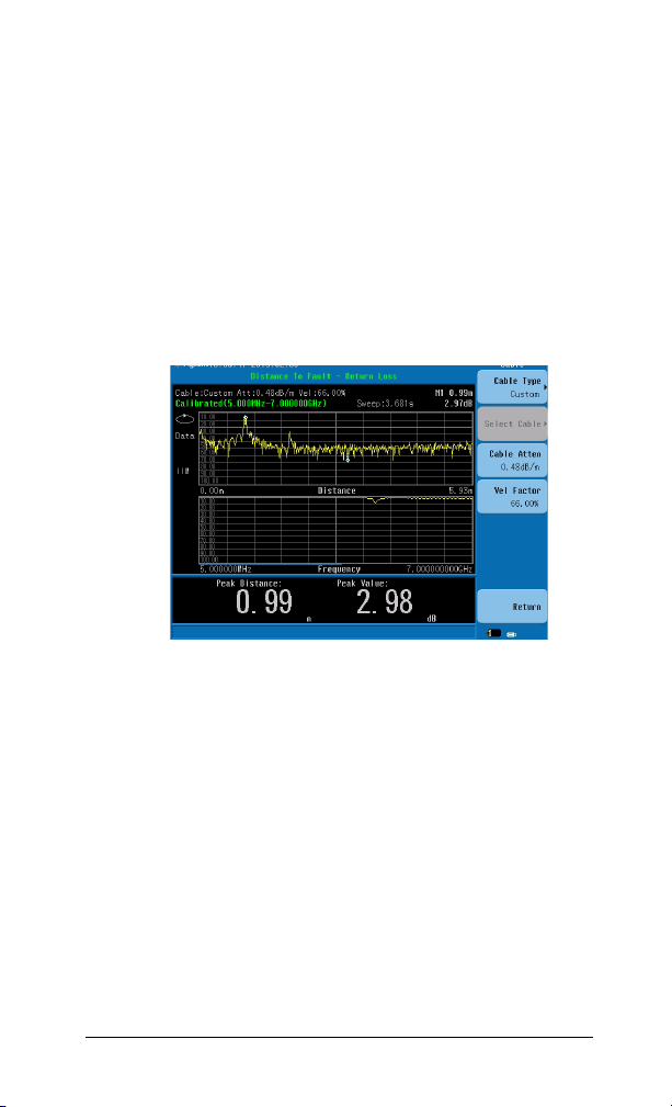
Functions and Measurements

{Cable Atten} and velocity factor by {Vel Factor}. In this example, the cable attenuation is 0.48 dB/meter and the velocity factor is 66%.

The DTF measurement starts and the results are displayed on the screen. A peak in the horizontal trace indicates a defective location.

Press [Meas] > {Freq Domain On} to enable the split screen with cable loss trace in frequency domain.

Figure 36 Frequency Domain Split Screen In DTF Test

Cable & Antenna Test

Measurement Functions

The cable and Antenna test mode provides the following measurement functions to help you with the complicated field test tasks.

Trac e M a th

Trace math provide a trace comparison function for your test. Press [Trace] > {Data->Mem} to save the current trace in yellow to the internal memor y in blue. Press {Data}, {Memory} or {Data&Memory} to display the corresponding traces on the screen.

Press {Trace Math} to choose the calculation types

for the trace comparison: {Data+Mem}, {Data-Mem}

Functions and Measurements

Cable & Antenna Test

and {Data/Mem}. The result is shown on the screen

in logarithmic power.

Press {Data&Memory} to show the trace math result in yellow and the saved trace in blue as Figure 37.

Figure 37 Trace Math In Distance To Fault Test

Press {A the current trace in yellow.

verage On} to turn on the trace average for

Interference Immunity

Interference immunity function is provided to filter the interference signal. This function key is available in all the measurement modes, including Reflection Measurement, One Port Cable Loss and Distance To Fault. Press {IIM On/Off} to toggle this function on and off.

Pass & Fail Test with Limit and Limit line

Press [Shift] > [Limit/Trace] to use the limit function for pass & fail test. There are two limits configuration which allows you to set the upper limit and lower limit for the trace. Press {Limit 1/2} > {Type} to toggle the limit direction between upper and lower. Press {Edit Limits} to set the limit points one by one. Then, press {Return} > {Limit on/off} to

Functions and Measurements

turn on the customized limit function. Then, the pass and fail indicator is displayed on the screen according to the customized criteria.

Press {Limit 1/2} > {Limit Line} to set a single limit line. Input the limit value and then press {Limit Line On} to enable the limit line as Figure 38.

Press {Limit Beep} to turn on the beep indicator. If the trace is failed to pass the limit line, there will be continuous beep indicating the failure.

Figure 38 Limit Line in Reflection Measurement

Cable & Antenna Test

Functions and Measurements

File Operation

Pressing [File] accesses a menu that allows you to manage file saving and loading.

Viewing a file list

Refer to the following two steps to view a file list:

1 Select the directory to view.

Press [File] > {Directory} > {Media Type} to toggle the displayed file list from internal memory, external USB memory stick or system memory.

2 Select the file type you wish to view.

Press [File] > {View FileType} to select a file type.

File Types

Each file type has a specific purpose as defined below:

• Trace ( * . D AT)

A trace file records trace data and controls.

• Screen (*.JPG)

A screen file records graphic information of the current screen.

• State (*.STA)

A state file records the current controls and settings of the analyzer. Use this file type for saving test parameters for future recall, such as Frequency, Amplitude and BW settings.

• Limit (*.LIM)

A limit file records the limit settings. You can edit the limit file and transfer this file between the N934xC and PC software.

• CSV (*.CSV)

A CSV file records the trace data and available for review on PC. With option GPS, you can convert the CSV file into KML file in HSA PC software for review the GPS location in Google Earth on PC.

Functions and Measurements

• Task Planner (*.TPF)

A task planner file contains the user- defined measurement tasks in sequence which make the test task easier in field test.

• Setup (*.SET)

A setup file records the system setting information, such as language, date/time, and power saving mode. This file type is not used for test parameter setup information.

• Standard (*.STD)

A standard file contains the frequency range and corresponding parameters for a specific communication standard. It allows you to recall those default settings for the singal searching and testing in that range.

• Amplitude Correction (*.COR)

The amplitude correction file is used for trace amplitude offset compensation. Please refer to

“Correction” on page 98 to edit and save the

correction file on HSA PC software.

• KML (*.KML)

A KML file is available for Google Earth on PC. It is specified for channel scanner measurement and the GPS location is only available when the option GPS is activated.

Figure 39 Review the KML file in Google Earth

File Operation

Functions and Measurements

NOTE

File Operation

Saving a file

Refer to the following three steps to save a file: 1 Press [File] > {Directory} > {Media Type} to select the

file directory.

2 Press [File] > {Save as}, The pop- up window

displays for your further setting.

3 Edit a file name.

A file name can consist of letters and digits. A sing le key stroke on the numerical keypad inputs a digital number; and consecutive key stroke selects and inputs a letter.

4 Rotate the knob to choose the file type you need.

5 Press [Enter] to save the file.

When a file saving completes, the saved file will display in the file list..

When a file is selected, you can edit the file name by pressing the numeric and alphabetic hardkeys on the right side of the analyzer’s front panel.

Quick Saving a File

Press [Save] to quickly save a trace or a screen to either the local memory or an external USB device, depending upon the setup of the save path.

Refer to the steps for saving a trace/screen:

1 Press [File] > {Setup} > {Qsave Type} to set the quick

save file type.

2 Press [File] > {Directory} > {Media Type} to select the

file directory.

3 Press [Return], [Save] to save a trace or a screen

copy to the pre- defined memory. The trace or screen will be automatically assigned with a default file name. A trace will be assigned with a file name, such as HYTRACE, HYTRACE_1, and consecutive decimal numbers appended to the alphabetic file name, such as HYSCREEN, HYSCREEN_1 and consecutive decimal numbers appended to the alphabetic file name.

Used Agilent Agilent Used N9342C Manual

Specifications and Main Features

Frequently Asked Questions

User Manual

Overview

Introduction

Functionality and Feature

Optimized Usability

Front Panel Overview

Display Annotations

Top Panel Overview

Instrument Markings

Getting Started

Checking Shipment and Order List

Power Requirements

AC Power Cords

Safety Considerations

Environmental Requirements

Electrical Requirements

Electrostatic Discharge (ESD) Precautions

Working with Batteries

Installing a Battery

Viewing the Battery Status

Charging a Battery

Powering the Analyzer on for the First Time

Preparation for Use

Power On and Preset Settings

Factory Default Settings

Visual and Audio Adjustment

General System Settings

Timed Power On/Off

IP configuration

Ext Input

Show System

Adding an Option

Show Error

Perform Calibration

Data Securities

Upgrading Firmware

Probe Power Output

HSA and BSA PC software

Making Basic Measurements

Viewing a Signal on the Analyzer

Figure 2-1 View a signal (1 GHz, 0 dBm)

Functions and Measurements

Measuring Multiple Signal s

Comparing Signals on the Same Screen

Figure 3 Del ta pair marker with signals (same screen)

Resolving Signals of Equal Amplitude

Figure 4 Setup for obtaining two signals

Figure 5 Resol ving signals of equal amplitude

Figure 6 Resol ving a small signal hidden by a larger signal

Measuring a Low-Level Signal

Figure 7 A signal closer to the noise level (Atten: 10 dB)

Figure 8 A signal closer to the noise level (Atten: 20 dB)

Figure 9 A signal closer to the noise level (Atten: 0 dB)

Decreasing the Resolution Bandwidth

Figure 10 Decreasing resolution band width

Figure 11 Using the average detector

Tra ce Av era gin g

Figure 12 Trace averaging

Improving Frequency Resolution and Accuracy

Figure 13 Using the frequency counter

Making Distortion Measurements

Identifying Analyzer Generated Distortion

Figure 14 Harmonic d istortion

Figure 15 Identifying Analyzer Distortion (O dB atten)

Figure 16 Identifying Analyzer Distortion (10 dB atten)

Third-Order Intermodulation Distortion

Figure 17 TOI test screen

Making a Stimulus Response Transmission Measurement

Figure 18 Transmission Measurement Test Setup

Figure 19 Measure the Rejection Range

Measuring Stop Band Attenuation of a Low-pass Filter

Figure 20 Minimum Stop Band Attenuation

Making a Reflection Calibration

Figure 22 Short Circuit Normalized

Measuring Return Loss Using the Reflection Calibration Routine

Figure 23 Measuring the Return Loss of the Filter

Making a Power Measurement with USB Power Sensor