Used Agilent Agilent Used N9320B Manual

Download

Page 1

Test Equipment Depot - 800.517.8431 - 99 Washington Street Melrose, MA 02176 - TestEquipmentDepot.com

Keysight N9320B Spectrum Analyzer

Notice: This document contains references to Agilent. Please note that Agilent’s Test and M

easurement business has become Keysight

Technologies.

User’s Guide

Page 2

Notices

No part of this manual may be reproduced in any form or by any means (including electronic storage and retrieval or translation into a foreign language) without prior agreement and written consent from Keysight Technologies, Inc. as governed by United States and international copyright laws.

Trademark Acknowledgments

Manual Part Number

N9320-90007

Edition

Edition 4, June 2014

Printed in China

Published by: Keysight Technologies

No 116 Tianfu 4th street Chiengdu, 610041 China

Warranty

THE MATERIAL CONTAINED IN THIS DOCUMENT IS PROVIDED “AS IS,” AND IS SUBJECT TO BEING CHANGED, WITHOUT NOTICE, IN FUTURE EDITIONS. FURTHER, TO THE MAXIMUM EXTENT PERMITTED BY APPLICABLE LAW, KEYSIGHT DISCLAIMS ALL WARRANTIES, EITHER EXPRESS OR IMPLIED WITH REGARD TO THIS MANUAL AND ANY INFORMATION CONTAINED HEREIN, INCLUDING BUT NOT LIMITED TO THE IMPLIED WARRANTIES OF MERCHANTABILITY AND FITNESS FOR A PARTICULAR PURPOSE. KEYSIGHT SHALL NOT BE LIABLE FOR ERRORS OR FOR INCIDENTAL OR CONSEQUENTIAL DAMAGES IN CONNECTION WITH THE FURNISHING, USE, OR PERFORMANCE OF THIS DOCUMENT OR ANY INFORMATION CONTAINED HEREIN. SHOULD KEYSIGHT AND THE USER HAVE A SEPARATE WRITTEN AGREEMENT WITH WARRANTY TERMS

COVERING THE MATERIAL IN THIS DOCUMENT THAT CONFLICT WITH THESE TERMS, THE WARRANTY TERMS IN THE SEPARATE AGREEMENT WILL CONTROL.

Technology Licenses

The hardware and/or software described in this document are furnished under a license and may be used or copied only in accordance with the terms of such license.

U.S. Government Rights

The Software is “commercial computer software,” as defined by Federal Acquisition Regulation (“FAR”) 2.101. Pursuant

12.212 and 27.405-3 and Department of Defense FAR Supplement (“DFARS”) 227.7202, the U.S. government acquires commercial computer software under the same terms by which the software is customarily provided to the public. Accordingly, Keysight provides the Software to U.S. government customers under its standard commercial license, which is embodied in its End User License Agreement (EULA). The license set forth in the EULA represents the exclusive authority by which the U.S. government may use, modify, distribute, or disclose the Software. The EULA and the license set forth therein, does not require or permit, among other things, that Keysight: (1) Furnish technical information related to commercial computer software or commercial computer software documentation that is not customarily provided to the public; or (2) Relinquish to, or otherwise provide, the government rights in excess of these rights customarily provided to the public to use, modify, reproduce, release, perform, display, or disclose commercial computer software computer software

to FAR

or commercial

documentation. No additional government requirements beyond those set forth in the EULA shall apply, except to the extent that those terms, rights, or licenses are explicitly required from all providers of commercial computer software pursuant to the FAR and the DFARS and are set forth specifically in writing elsewhere in the EULA. Keysight shall be under no obligation to update, revise or otherwise modify the Software. With respect to any technical data as defined by FAR 2.101, pursuant to FAR 12.211 and 27.404.2 and DFARS 227.7102, the U.S. government acquires no greater than Limited Rights as defined in FAR 27.401 or DFAR 227.7103-5 (c), as applicable in any technical data.

Safety Notices

A CAUTION notice denotes a hazard. It calls attention to an operating procedure, practice, or the like that, if not correctly performed or adhered to, could result in damage to the product or loss of important data. Do not proceed beyond a CAUTION notice until the indicated conditions are fully understood and met.

A WARNING notice denotes a hazard. It calls attention to an operating procedure, practice, or the like that, if not correctly performed or adhered to, could result in personal injury or death. Do not proceed beyond a WARNING notice until the indicated conditions are fully understood and met.

Page 3

1 Overview 1

Keysight N9320B at a Glance 2

Front Panel Overview 4

Rear Panel Overview 9

Front and rear panel symbols 10

2 Getting Started 11

Check the Shipment and Order List 12

Safety Notice 14

Power Requirements 15

Power On and Check 17

Environmental Requirements 19

South Korea Class A EMC Declaration 22

Helpful Tips 23

Perform a Self Alignment 23

Perform a Time Base Calibration 23

Using an External Reference 24

Enable an Options 24

Firmware Upgrade 25

IO Configuration 25

Power Preset Last 26

3 Functions and Measurements 27

Making a Basic Measurement 28

Using the Front Panel 28

Presetting the Spectrum Analyzer 29

Page 4

Contents

Viewing a Signal 30

Measuring Multiple Signals 32

Comparing Signals on the Same Screen Using Marker Delta 32

Comparing Signals not on the Same Screen Using Marker Delta 34

Resolving Signals of Equal Amplitude 36

Resolving Small Signals Hidden by Large Signals 39

Measuring a Low-Level Signal 41

Reducing Input Attenuation 41

Decreasing the Resolution Bandwidth 43

Trace Averaging 44

Improving Frequency Resolution and Accuracy 46

Tracking Drifting Signals 48

Making Distortion Measurements 50

Identifying Analyzer Generated Distortion 50

Third-Order Intermodulation Distortion 53

Measuring Phase Noise 56

Stimulus Response Transmission 57

Measuring Stop Band Attenuation of a Lowpass Filter 60

Making a Reflection Calibration Measurement 63

Measuring Return Loss Using the Reflection Calibration Routine 66

Making an Average Power Measurement 67

Demodulate the AM/FM signal 71

Demodulating an AM Signal 71

Demodulating an FM Signal 72

Page 5

Analysis the Modulated Signals 74

AM/FM Modulation Analysis 74

ASK/FSK Modulation Analysis 77

Measuring Channel Power 80

Viewing Catalogs and Saving Files 83

Locating and Viewing Files in the Catalog 83

Saving a File 84

Loading a File 86

Copying a File 87

Deleting a File 87

4 Key Reference 89

Amplitude 90

Auto Tune 94

Contents

Back <- 95

BW/Avg 96

Det/Display 100

Enter 106

File 107

Frequency 113

Marker 115

Marker-> 121

Meas 122

Channel Power 122

Occupied BW 124

ACP 127

Page 6

Contents

Intermod (TOI) 130

Spectrum Emission Mask 132

MODE 139

Tracking Generator 139

Power Meter 143

AM/FM Modulation Analysis 146

ASK/FSK Modulation Analysis 150

Peak Search 154

Preset/System 158

SPAN 164

Sweep/Trig 166

Trace 168

5 Instrument Messages 171

Overview 172

Command Errors 173

Execution Conflict 175

Device-Specific Errors 177

6 Troubleshooting 181

Check the basics 182

Contact Keysight Technologies 184

Index 207

Page 7

7 Menu Maps 185

Amplitude Menu 186

BW/Avg Menu 187

Det/Display Menu 188

File Menu (1 of 2) 189

File Menu (2 of 2) 190

Frequency Menu 191

Marker Menu 192

Marker-> Menu 193

Measure Menu (1 of 2) 194

Measure Menu (2 of 2) 195

MODE - Tracking Generator 196

MODE - Power Meter 197

Contents

MODE - AM/FM Modulation Analysis 198

MODE - ASK/FSK Modulation Analysis 199

Name Editor Menu 200

Peak Search Menu 201

Preset/System Menu 202

SPAN Menu 203

Sweep/Trig Menu 204

Trace Menu 205

Page 8

Contents

Page 9

Overview

1 Overview

Keysight N9320B at a Glance 2

Front Panel Overview 4

Rear Panel Overview 9

Front and rear panel symbols 10

This chapter provides a description of the Keysight N9320B spectrum analyzer and an introduction to the buttons, features, and functions of the front and rear instrument panels.

Page 10

Overview Keysight N9320B at a Glance

Keysight N9320B at a Glance

The Keysight N9320B spectrum analyzer is a portable, swept spectrum can be a fundamental component of an automated system. It can also be widely used in an electronic manufacturing environment and in functional/final/QA test systems.

Features

The Keysight N9320B spectrum analyzer primary features and functions are described below:

• High Sensitive Measurement

The spectrum analyzer includes an optional pre-amplifier for signals in the frequency range up to 3 GHz, enabling more sensitive measurements. This feature is a great help in analysis of weaker signals.

• High Accuracy Power Measurement

analyzer with a frequency range of 9 kHz to 3.0 GHz. It

The N9320B supports Keysight U2000 series power sensors for high accuracy power measurement as a power meter.

• Power Measurement Suite

The built-in one-button power measurement suite offers channel power, ACP, OBW, and TOI measurements.

• Spectrum Emission Mask

provides a Pass/Fail testing capability with a mask for out-of-channel emissions measurement.

Page 11

Overview

Keysight N9320B at a Glance

• Modulation Analysis Function

provides optional AM/FM and ASK/FSK modulation analysis function. (AM/FM: Option-AMA ASK/FSK: Option-DMA)

• Tracking Generator

provides an RF source for scalar network analysis (Option-TG3).

Page 12

Overview

Local

Save

PROBE POWER

RF IN 50

50VDC MAX 30dBm 1W MAX

TG SOURCE CAL OUT

50MHz 10dBm

Remot e

Standby On

102

596

Back

Frequency

SPAN

Marker

Peak Search

Marker

Auto Tune

Det/ Display

File/ Print

BW/ Avg

View/ Trace

MeasMODE

Preset/ System

Amplitude

Enter

Sweep/ Trig

N9320B 9 kHz - 3.0 GHz

SPECTRUM ANALYZER

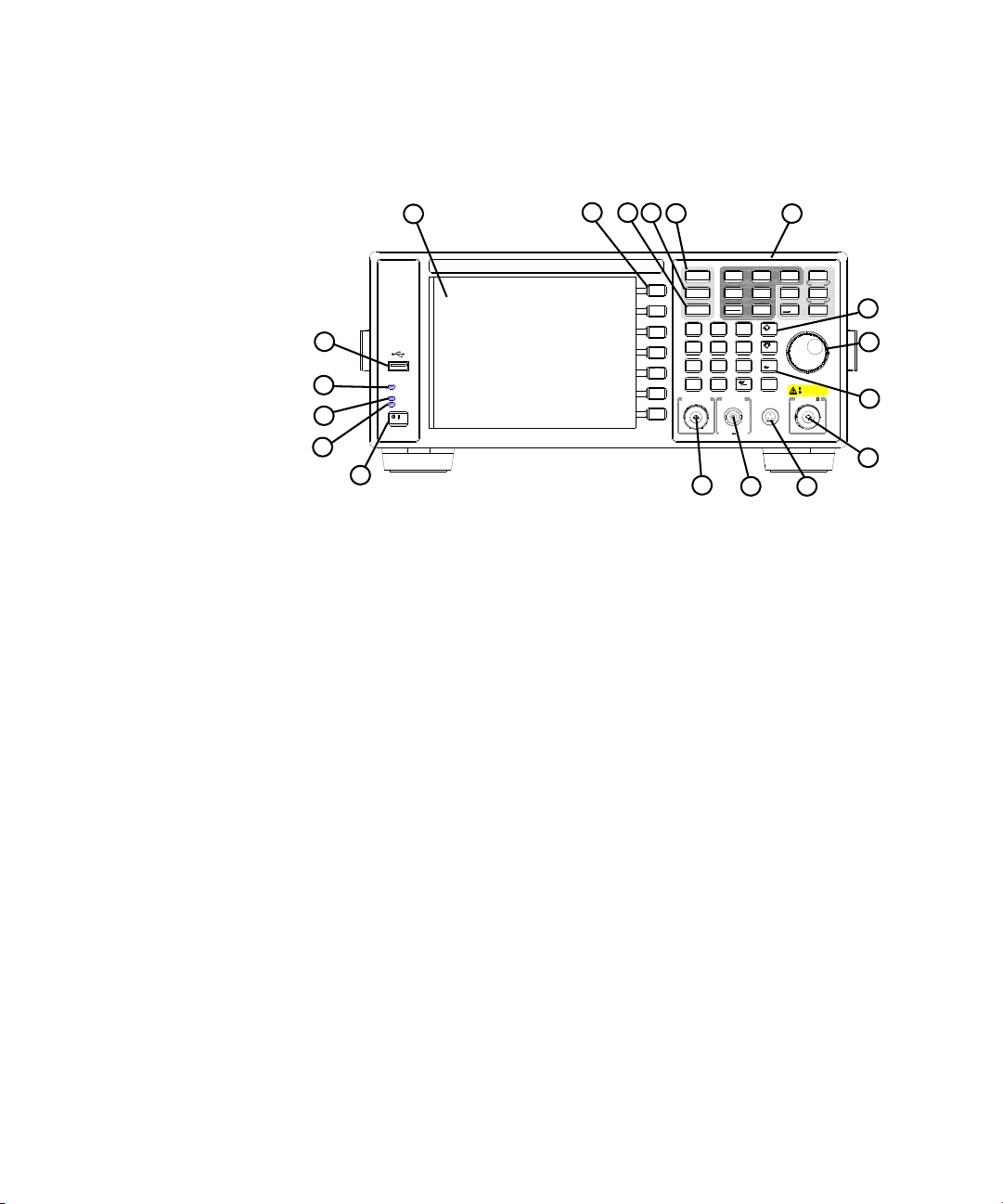
Front Panel Overview

1Screen 6.5 inch TFT color screen shows information of the

current function, including the signal traces, status indicators, and instrument messages. Labels for softkeys are located on the right-hand side of the screen.

2 Softkeys are the unlabeled keys next to the screen. They activate

functions displayed to the left of each key.

3 Amplitude activates the reference level function and accesses

the amplitude softkeys, with which you set functions that affect data on the vertical axis.

4 SPAN sets the frequency range symmetrically about the center

frequency. The frequency-span readout describes the total displayed frequency range.

5 Frequency activates the center-frequency function, and accesses

the menu of frequency functions.

6 Function Keys relate directly to the following main functions:

• Preset/System (Local) accesses the softkeys to reset the

analyzer to a known state, if the analyzer is in the remote mode, pressing this key returns the analyzer to the local mode and enables front-panel control.

Page 13

Overview

Front Panel Overview

• Auto Tune searches the signal automatically and locates the

signal to the center of the graticule. see

page 94

• BW/Avg activates the resolution bandwidth function and

accesses the softkeys that control the bandwidth functions and averaging.

• Sweep/Trig accesses the softkeys that allow you to set the

sweep time, select the sweep mode and trigger mode of the analyzer.

• View/Trace accesses the softkeys that allow you to store and

manipulate trace information.

• Det/Display accesses the softkeys that allow you to configure

detector functions and control what is displayed on the analyzer, including the display line, graticule and annotation, as well as the testing of trace data against entered limits.

• MODE selects the measurement mode of your analyzer.

• Meas accesses the softkeys that let you make transmitter

power measurements such as adjacent channel power, occupied bandwidth, and harmonic distortion, etc.

• Marker accesses the marker control keys that select the type

and number of markers and turns them on and off.

• Marker accesses the marker function softkeys that help you

with the measurement.

• Peak Search places a marker on the highest peak.

• File accesses the softkeys that allow you to configure the file

system of the analyzer.

"Auto Tune" on

7 Arrow Keys The up and down arrow keys shift the selected item

when you press [MODE] hardkey; you can also change the mode by rotating the knob.

8 Knob The front panel knob increases or decreases a value, a

numeric digit, or scrolls up and down to select an item in a list.

Page 14

Overview

CAUTION

Front Panel Overview

9 Data Control Keys includes the numeric keypad, ENTER key and

backspace key, change the numeric value of an active function such as center frequency, start frequency, resolution bandwidth, and marker position.

10 RF IN connector is the signal input for the analyzer. The

maximum damage level is average continuous power +40 dBm, DC voltage 50 VDC or max pulse voltage 125 V. The impedance is 50  (N-type female).

11 PROBE POWER connector provides power for high-impedance

AC probes or other accessories (+15 V, –12 V, 150 mA maximum).

12 CAL OUT connector provides an amplitude reference signal

output of 50 MHz at –10 dBm (BNC female).

13 TG SOURCE connector N-type female, is the source output for

the built-in tracking generator. The impedance is 50 . (for Option TG3)

If the tracking generator output power is higher than the maximum power that the device under test can tolerate, it may damage the device under test. Do not exceed the maximum power of DUT.

14 Standby Switch switches on all functions of the analyzer. To

switch the analyzer off, press the switch for at least 2 seconds. This deactivates all the functions but retains power to internal circuits so long as the analyzer is connected to line power.

15 On LED (green) lights when the analyzer is switched on.

16 Standby LED (orange) lights when the analyzer is connected to

the line power.

17 Remote LED lights when the analyzer is remotely controlled by a

PC via the USB host interface on the rear panel.

18 USB Device Connector provides a connection between external

USB devices and the analyzer, such as a USB memory device.

Page 15

Display Annotations

1819

Overview

Front Panel Overview

Item Description Notes (Associated function key)

1 Amplitude scale [Amplitude] > Scale Type

2 Detector mode [Det/Display] > Detector

3 Reference level [Amplitude]

4 Active function block The function in use

5 Time and date display [Preset/System] > Time/Date

6 RF attenuation [Amplitude] > Attenuation Auto

7 Marker frequency [Marker] or

> Ref Level

[Marker] > Function > Frequency

Counter

8 Uncal indicator The readout of amplitude is

uncalibrated.

9 Marker amplitude [Marker]

10 External reference An external frequency reference is in use.

Page 16

Overview Front Panel Overview

11 Remote mode The analyzer is in remote mode

12 Key menu title Dependent on key selection.

13 Softkey menu Refer to

Dependent on current function key

selection.

14 Frequency span [SPAN]

15 Sweep time [Sweep/Trig] > Sweep Time

16 Video bandwidth [Bw/Avg] > Video BW

17 Display status line Display status and instrument messages.

18 Resolution bandwidth [Bw/Avg] > Res BW

19 Trigger/Sweep

F - free run trigger L - line trigger V - video trigger E - external trigger C - continuous sweep S - single sweep

20 Continuous peak [Peak Search] > Continuous pk

21 Signal track [SPAN] > Span

22 Internal preamp [Amplitude] > Int Preamp

23 Key menu title Dependent on key selection

24 Trace mode

W - clear write M - maximum hold m - minimum hold V - view S - store blank

25 Average

VAvg - video average PAvg - power average

26 Display line [Det/Display] > display Line On Off

[Sweep/Trig]

[Trace]

[Bw/Avg] > Average On Off

"Key Reference" for details.

Page 17

Rear Panel Overview

REF IN

REF OUT

TRIG IN

USB

LAN

VGA OUT

T T L

~100-240

50-60

100

W MAX

SERIAL LABEL ATTACH HERE

HIPOT LABEL ATTACH HERE

10MHz

GPIB

1 REF OUT connector provides a frequency of 10 MHz, amplitude of

2 REF IN connector accepts an external timebase with a frequency

3 Kensington Lock lock the instrument and keep its safety. 4 LAN port A TCP/IP Interface that is used for remote analyzer

5 EXT TRG IN (TTL) connector accepts an external voltage input,

6 Power switch isolates the analyzer from the AC line power. After

7 AC Power Receptacle accepts a three-pin line power plug.

Overview

Rear Panel Overview

–10 dBm reference output. (BNC female)

of 10 MHz, amplitude of –5 to +10 dBm. (BNC female)

operation.

the positive edge of which triggers the analyzer sweep function. (BNC female)

switch on, the analyzer enters into standby mode and the orange standby LED on the front panel lights.

8 VGA connector provides the video output signal to an external

monitor or projector. (D-sub 15-pin female)

9 USB Host connector provides a connection between the analyzer

and an PC for remote control.

10 GPIB connector (Option G01) is an optional interface. GPIB

supports remote analyzer operation.

Page 18

Overview

ISM1-A

ICES/NMB-001

Front and rear panel symbols

Instruction manual symbol: indicates that the user must refer to specific instructions in the manual.

CE mark: a registered trademark of the European Community.

Shows that this is an Industrial Scientific and Medical Group 1 Class A product. (CISPR 11, Clause 4)

The CSA mark: a registered trademark of the Canadian Standards Association International.

The ISM device complies with Canadian Interference-Causing Equipment Standard-001. Cet appareil ISM est conforme à la norme NMB-001 du Canada.

All Level 1, 2 or 3 electrical equipment offered for sale in Australia and New Zealand by Responsible Suppliers must be marked with the Regulatory Compliance Mark (RCM Mark).

marks the “on/standby” position of the switch.

indicates that the instrument requires AC power input.

indicates this product complies with the WEEE Directive(2002/96/EC) marking requirements and you must not discard this equipment in domestic household waste. Do not dispose in domestic household waste.

indicates the time period during which no hazardous or toxic substance elements are expected to leak or deteriorate during normal use. Forty years is the expected useful life of the product.

KC mark: as Korea Certification. This equipment is Class A suitable for professional use and is for use in electromagnetic environments outside of the home.

Page 19

Getting Started

2 Getting Started

Check the Shipment and Order List 12

Safety Notice 14

Power Requirements 15

Power On and Check 17

Environmental Requirements 19

South Korea Class A EMC Declaration 22

Helpful Tips 23

This chapter helps you in preparing the spectrum analyzer for use and provides the information to start using the spectrum analyzer correctly.

Page 20

Getting Started Check the Shipment and Order List

Check the Shipment and Order List

After receiving the shipment, first check the shipment and your order list.

Inspect the shipping container and the cushioning material for signs of stress. Retain the shipping materials for future use, as you may wish to ship the analyzer to another location or to Keysight Technologies for service. Verify that the contents of the shipping container are complete.

Each spectrum analyzer includes the following accessories as standard:

Item Description

USB cable (A-B) Connection for remote control

N-BNC adapter and BNC cable Connection for alignment

Three-pin power cord Specific to shipping location

Help kit CD-ROM HSA and BSA PC Software

Keysight IO libraries suite N9320B documentation

Shipping Problems?

If the shipping materials are damaged or the contents of the container are incomplete:

• Contact the nearest Keysight Technologies office to arrange for repair or replacement. You will not need to wait for a claim settlement.

• Keep the shipping materials for the carrier’s inspection.

• If you must return an analyzer to Keysight Technologies, use the original (or comparable) shipping materials.

For any questions about your shipment, please contact Keysight Technologies for consulting and service.

Page 21

Options

Getting Started

Check the Shipment and Order List

Verify if that the shipment includes your ordered options by checking the option label on the shipping container:

Option Description Part number

PA3 3 GHz Preamplifier N9320B-PA3 G01 GPIB interface N9320B-G01 AMA AM/FM demodulation N9320B-AMA DMA ASK/FSK demodulation N9320B-DMA TG3 3 GHz tracking generator N9320B-TG3 EMF EMI filter N9320B-EMF G01 GPIB interface N9320B-G01 TR1 RF training kit N9320B-TR1 1HB Handle and bumpers N9320B-1HB 1CM Rackmount kit N9320B-1CM 1TC Hard transit case N9320B-1TC UK6 Commercial calibration certificate

with testing data

N9320B-UK6

Unless specified otherwise, all options are available when you order a spectrum analyzer; some options are also available as kits that you can order and install/activate after you receive the analyzer. Order kits through your local Keysight Sales and Service Office.

At the time of analyzer purchase, options can be ordered using your product number and the number of the option you are ordering. For example, if you are ordering option TG3, you would order N9320B-TG3.

If you are ordering an option after the purchase of your analyzer, you will need to add a K to the product number and then specify which option you are ordering. For example, N9320BK-TG3.

Page 22

Getting Started

WARNING

CAUTION

Safety Notice

Read the following warnings and cautions carefully before powering on the spectrum analyzer to ensure personal and instrument safety.

Always use a well-grounded, three-pin AC power cord to connect to power source. Personal injury may occur if there is any interruption of the AC power cord. Intentional interruption is prohibited. If this product is to be energized via an external auto transformer for voltage reduction, make sure that its common terminal is connected to a neutral (earthed pole) of the power supply.

Personal injury may result if the spectrum analyzer covers are removed. There are no operator-serviceable parts inside. To avoid electrical shock, refer servicing to qualified personnel.

Electrical shock may result if the spectrum analyzer is connected to the power supply while cleaning. Do not attempt to clean internally.

Prevent damage to the instrument and ensure protection of the input mixer by limiting average continuous power input to +33 dBm, DC voltage to 50 VDC with > Instrument damage may result if these precautions are not followed.

To install the spectrum analyzer in other racks, note that they may promote shock hazards, overheating, dusting contamination, and inferior system performance. Consult your Keysight customer engineer about installation, warranty, and support details.

10 dB input attenuation.

Page 23

Power Requirements

AC Power Cord

Getting Started

Power Requirements

The spectrum analyzer has an auto-ranging line voltage input. The AC power supply must meet the following requirements:

Voltage: 100 to 240 VAC (90 to 264 VAC)

Frequency: 50 to 60 Hz

Power: Maximum 100 W

The analyzer is equipped with a three-wire power cord, in accordance with international safety standards. This cable grounds the analyzer cabinet when connected to an appropriate power line outlet. The cable appropriate to the original shipping location is included with the analyzer.

Various AC power cables are available that are unique to specific geographic areas. You can order additional AC power cables for use in different areas. The table AC Power Cords lists the available AC power cables, the plug configurations, and identifies the geographic area in which each cable is appropriate.

The detachable power cord is the product disconnecting device. It disconnects the mains circuits from the mains supply before other parts of the product. The front panel switch is only a standby switch and do not disconnect instrument from LINE power.

Page 24

Getting Started

250V 10A

250V 16A

230V 15A

250V 16A

Power Requirements

AC Power Cords

Plug Type Cable Part

Number

8121-1703 BS 1363/A Option 900

8120-0696 AS

8120-1692 IEC 83 C4 Option 902

8120-1521 CNS 10917-2

125V 10A

8120-2296 SEV 1011 Option 906

250V 10A

8120-4600 SABS 164-1 Option 917

8120-4754 JIS C8303 Option 918

125V 15A

Plug Description

3112:2000

/NEMA 5-15P

For use in Country & Region

United Kingdom, Hong Kong, Singapore, Malaysia

Option 901

Australia, New Zealand

Continenta l Europe, Korea, Indonesia, Italy, Russia

Option 903

United States, Canada, Tai w an, M e xico

Switzerland

South Africa, India

Japan

8120-5181 SI 32 Option 919

Israel

8120-8377 GB 1002 Option 922

China

250V 10A

a. Plug description describes the plug only. The part number is for the complete cable assembly.

Page 25

Power On and Check

NOTE

1 Connect the AC power cord into the instrument. Insert the plug

2 Press the AC line switch on the rear panel. The standby LED on

Getting Started

Power On and Check

into a power socket provided with a protective ground. Set the tilt adjustors for your preference.

Figure 1 Plug in and angle adjustment

the front panel will light and the spectrum analyzer is in standby mode (AC power applied).

3 Press the standby switch on the front panel. The On LED will

light, and the spectrum analyzer boots up.

Self-initialization takes about 25 seconds; the spectrum analyzer then defaults to the menu mode. After power on, let the spectrum analyzer warm up for 45 minutes for stabilization.

The front panel switch is a standby switch only; it is not a power switch. To completely disconnect the spectrum analyzer from the AC line power, shut off the power switch on the rear panel.

Page 26

Getting Started

Preset/ System

Power On and Check

Running Internal Alignments

Check for Instrument Messages

To meet the instrument performance specifications, the analyzer must periodically be manually aligned.

1 Connect a BNC cable with the N-BNC adapter between the CAL

OUT and RF IN front panel connectors.

2 After 15-minute warm up, press > Alignment > Align > All

The self alignment takes about 5 minutes.

When an alignment is being run, there will be an audible clicking sound as the attenuator settings are changed. This sound is not an indication of a problem.

Please refer to

"Alignment" on page 159 for further information.

The spectrum analyzer has two categories of instrument messages: error and warning messages. A error message is triggered by operation errors, for example, parameter setting conflicts or data input that is out of the range of a parameter. An warning message may be triggered by hardware defects which could result in damage to instrument.

Here are some tips to check the instrument messages.

1 Check the display to see if any messages display in the status bar.

Press > More > Show Errors to review each message. Refer to

Chapter 5, "Instrument Messages" for detailed system message

descriptions.

2 When you have reviewed and resolved all of the error messages,

press > More > Show Errors > Clear error queue to delete the messages.

3 Cycle the power to the analyzer and re-check to see if the

instrument messages are still there.

4 If the error messages cannot be resolved, please contact the

Keysight Customer Contact Center for assistance or service.

Page 27

Environmental Requirements

Keysight Technologies has designed this product for use in Installation Category II, Pollution Degree 2, per IEC 61010-1. Keysight has designed the spectrum analyzer for use under the following conditions:

• Indoor use

• Altitude < 3,000 meters

• Operating temperature range: +5 to +45

Storage temperature range: –20 to +70

• Relative humidity range 15% to 95% at 40

Ventilation

Ventilation holes are located on the rear panel and one side of the spectrum analyzer cover. Do not allow these holes to be obstructed, as they allow air flow through the spectrum analyzer.

When installing the spectrum analyzer in a cabinet, do not restrict the convection of the analyzer. The ambient temperature outside the cabinet must be less than the maximum operating temperature of the spectrum analyzer by 4 within the cabinet.

Getting Started

Environmental Requirements

C for every 100 watts dissipated

Cleaning Tips

To prevent electrical shock, disconnect the spectrum analyzer from line power before cleaning. Use a dry cloth or one slightly dampened with water to clean the external case parts. Do not attempt to clean internally.

Page 28

Getting Started Environmental Requirements

Rack Mount

It is recommended to use the Keysight rackmount kit (option 1CM) to install the spectrum analyzer into a rack.

Do not attempt to rack mount the spectrum analyzer by the front panel handles only. This rackmount kit will allow mounting of the spectrum analyzer with or without handles.

Refer to the following instructions when installing the rackmount kit on the spectrum analyzer.

1 Remove feet, key-locks and tilt stands.

2 Remove side trim strips and one middle screw per side.

Page 29

Getting Started

CAUTION

Environmental Requirements

3 Attach rackmount flange and front handle assembly with 3 screws

per side.

4 Attach the spectrum analyzer to the rack using the rackmount

flanges with two dress screws per side.

Installing the spectrum analyzers into other racks may promote shock hazards, overheating, dust contamination, and inferior system performance. Consult your Keysight customer engineer about installation, warranty, and support details.

Page 30

Getting Started South Korea Class A EMC Declaration

South Korea Class A EMC Declaration

This equipment is Class A suitable for professional use and is for use in electromagnetic environments outside of the home.

Page 31

Helpful Tips

Preset/ System

Perform a Self Alignment

Getting Started

Helpful Tips

The following contains information to help in using and maintaining the instrument for optimum operation, including alignment, external reference, firmware update and option activation.

The N9320B provides a self alignment function to manually align the amplitude based on the time base. The analyzer should warm up for approximately 30 minutes before self alignment.

When the self aligment function is triggered, the current measurement is interrupted and a gauge displays on the LCD. The gauge simply indicates alignment is in process. When the aligment is finished, the interrupted measurement restarts.

Please refer to the operation procedures as below:

1 Connect a BNC cable with a N-BNC adapter between the CAL OUT

and RF IN front panel connectors.

2 Press > Alignment > Alignment > Align (Ext Cable) to initiate

the alignment.

Perform a Time Base Calibration

The N9320B provides a manual calibration function to calibrate the time base. The analyzer should warm up for approximately 30 minutes before calibration.

When the calibration function is triggered, the current measurement is interrupted and a gauge displays on the LCD. The gauge simply indicates calibration action rather than calibration course.

Page 32

Getting Started

Preset/ System

Helpful Tips

Please refer to the operation procedures as below:

1 Connect a 10 MHz reference TTL signal from external signal

generator to EXT TRG IN connectors on rear panel.

2 Press > Alignment > Timebase to initiate a calibration.

When the calibration is finished, the interrupted measurement restarts.

Using an External Reference

To use an external 10 MHz source as the reference frequency, connect the external reference source to the REF IN connector on the rear panel. An EXT REF indicator will display in the upper bar of the display. The signal level must be in the range of –5 to +10 dBm. When the reference signal is ready, the instrument switches the reference from time base to the external reference.

Enable an Options

Option license key information is required to enable product options. Contact your nearest Keysight office for purchasing a license. Refer to the procedures below to activate the options you have purchased.

1 Press > More > More > Licensing > Option

2 Enter the option number to be enabled. Press [Enter] to confirm

your input.

3 Press License key, enter the license key in the onscreen window.

Press [Enter] to confirm your input and terminate the license key input.

4 Press Activate License. The option

will be enabled immediately.

The analyzer provides the trial license with limited time usage of the interested options.

Page 33

Firmware Upgrade

Preset/ System

CAUTION

Preset/ System

Press > More > Show software to view the firmware revision of your analyzer. If you call Keysight Technologies regarding your analyzer, it is helpful to have this revision and the analyzer serial number available.

Follow this procedure to finish the firmware update:

1 Download the firmware package from web. Extract and copy the

file version and folder “n9320b” into the root directory of a USB stick.

2 Plug the USB stick into the connector. Press > Upgrade

The analyzer will perform the update process automatically. The upgrade procedure will take several minutes. Once the upgrade is completed, please follow the instruction to reboot the instrument.

Any interruption during the update process will result in update failure and system data lost. Do not remove the USB storage device until the update is finished.

Getting Started

Helpful Tips

IO Configuration

The N9320B spectrum analyzer provides three types of IO connnection: USB, LAN and optional GPIB interface. Press > {IO Configure} to select the corresponding interface as your need.

USB

Select USB to enable the USB connection for remote control.

LAN

The N9320B supports LAN port connection for remote control. Press > {More} > {More} > {IP Admin} to set the IP parameters for the network connection.

Page 34

Getting Started

Preset/ System

Helpful Tips

Press {IP Select Static} to manually set the IP address, gateway and subnet mask with the proper LAN information, or just press {IP Select DCHP} to set the IP address in LAN dynamically according DCHP.

Press {Apply} to enable all the parameters you set.

Press > {IO Configure} > {LAN} to enable the LAN connection according to the IP configuration you set.

GPIB

Press > {More} > {More} > {GPIB Address} to set the GPIB address for the analyzer.

Press > {IO Configure} > {GPIB} to enable the GPIB connection. The GPIB softkey is only vaild after the option G01 installed.

Power Preset Last

The option C20 provides the capability to save the last state of the analyzer before power off/power failed (essentially uplugging, replugging).

Press > {Pwr On/Preset} > {Power On Last} to activate this function. For the standard N9320B, this operation only save the last state if the analyzer is turned off by the front panel power switch.

Page 35

Functions and Measurements

3 Functions and Measurements

Making a Basic Measurement 28

Measuring Multiple Signals 32

Measuring a Low-Level Signal 41

Improving Frequency Resolution and Accuracy 46

Tracking Drifting Signals 48

Making Distortion Measurements 50

Measuring Phase Noise 56

Stimulus Response Transmission 57

Measuring Stop Band Attenuation of a Lowpass Filter 60

Making a Reflection Calibration Measurement 63

Measuring Return Loss with the Reflection Calibration Routine 66

Making an Average Power Measurement 67

Demodulate the AM/FM signal 71

Analysis the Modulated Signals 74

Measuring Channel Power 80

Viewing Catalogs and Saving Files 83

This chapter provides information on the analyzer functions and specific measurements capabilities of the spectrum analyzer.

Page 36

Functions and Measurements Making a Basic Measurement

Making a Basic Measurement

In this guide, the keys labeled with [ ], for example, [Preset/System] refer to front-panel hardkeys. Pressing many of the hardkeys accesses softkey menus that are displayed along the right side of the screen. The softkey menu labels are aligned so that they are located next to the softkeys at the right side of the display screen. For example, Preset is a softkey menu selection when first pressing [Preset/System].

Using the Front Panel

This section provides you with the information on using the front panel of the spectrum analyzer.

Entering Data

When setting the measurement parameters, there are several ways to enter or modify the value of the active function:

Knob Increments or decrements the current value.

Arrow Keys Increments or decrements the current value by a step unit.

Numeric Keys Enters a specific value. Then press the desired terminator (either a

unit softkey, or [Enter] hardkey).

Unit Softkeys Terminate (enter) a value with a unit softkey from the menu.

Enter Key Terminates an entry when no unit of measure is required, or the

instrument uses the default unit.

Back Key To delete

the current input digit prior to entering the value.

Using Softkeys

Softkeys are used to modify the analyzer function parameter settings. Some examples of softkey types are:

Toggle Turn on or off an instrument state.

Submenu Displays a secondary menu of softkeys, {More}.

Choice Selecting from a list of standard values or filenames.

Adjust Highlights the softkey and sets the active function.

Page 37

Functions and Measurements

Preset/ System

Making a Basic Measurement

Presetting the Spectrum Analyzer

Preset function provides a known instrument status for making measurements. There are two types of presets, factory and user:

Factory Preset When this preset type is selected, it restores the analyzer to its

factory-defined state. A set of known instrument parameter settings defined by the factory. Refer to “Factory Default Preset

State” on page 159 for details.

User Preset Restores the analyzer to a user-defined state. A set of user defined

instrument parameter settings saved for assisting the user in quickly returning to known a instrument measurement setup.

Press > Pwr on/Preset > Preset Type to select the preset type.

When Preset Type is set to Factory, pressing > Preset triggers a factory preset condition. The instrument will immediately return to the factory default instrument parameter setting.

When Preset Type is set to User, pressing > Preset displays both User Preset and Factory Preset softkeys. The user may then select the preset desired from the softkey menu selections.

Setting up a User Preset

To quickly return to instrument settings that are user defined, perform the following steps to save the instrument state as the user-defined preset:

1 Set the instrument parameters to the values and settings

necessary for the user preset state. This would include the frequency, span, amplitude, BW, and measurement type and any other setup details desired.

2 Press > Pwr on/Preset > Save User Preset, to save the

current instrument settings as the ‘user preset’ state. The user preset will not affect the default factory preset settings. User preset settings can be changed and saved at any time.

Page 38

Functions and Measurements

Preset/ System

Amplitud

Frequenc

SPAN

NOTE

Peak Search

Making a Basic Measurement

Viewing a Signal

1 Press > Pow on/Preset > Preset Type > Factory to enable the

2 Press > Preset to restore the analyzer to its factory-defined

3 Connect the 10 MHz REF OUT on the rear panel to the front-panel

1 Press > 10 > dBm to set 10 dBm reference level.

2 Press > 30 > MHz to set 30 MHz to center frequency.

Refer to the procedures below to view a signal.

factory-defined preset state.

state.

RF IN.

Setting the Reference Level and Center Frequency

Setting Frequency Span

Press > 50 > MHz to set 50 MHz frequency span.

Changing the reference level changes the amplitude value of the top graticule line. Changing the center frequency changes the horizontal placement of the signal on the display. Increasing the span will increase the frequency range that appears horizontally across the display.

Reading Frequency and Amplitude

1 Press to place a marker (labeled 1) on the 10 MHz peak.

Page 39

Functions and Measurements

Marker

10.000000 MHz

0.43 dBm

Active function block

Marker Annotation

Amplitude

Marker

NOTE

Making a Basic Measurement

Note that the frequency and amplitude of the marker appear both in the active function block, and in the upper-right corner of the screen.

Figure 3-1 10 MHz Internal Reference Signal

2 Use the knob, the arrow keys, or the softkeys in the Peak Search

menu to move the marker. The marker information will be displayed in the upper-right corner of the screen.

Changing Reference Level

1 Press and note that reference level (Ref Level) is now the

active function.

2 Press

Changing the reference level changes the amplitude value of the top graticule line.

> Mkr-> Ref Lvl.

Page 40

Functions and Measurements

Preset/ System

Frequenc

SPAN

Amplitud

Peak Search

Marker

Measuring Multiple Signals

This section provides the information on how to measure multiple signals.

Comparing Signals on the Same Screen Using Marker Delta

The delta marker function allows the user to compare two signals when both appear on the screen at the same time.

In the following example, harmonics of the 10 MHz reference signal available are used to measure frequency and amplitude differences between two signals on the same screen. Delta marker is used to demonstrate this comparison.

1 Preset the analyzer:

Press > Preset (With Preset Type of Factory)

2 Connect the rear panel REF OUT to the front panel RF IN.

3 Set the analyzer center frequency, span and reference level to view

the 10 MHz signal and its harmonics up to 50 MHz:

Press > 30 > MHz

Press > 50 > MHz

Press > 10 > dBm

4 Place a marker at the highest peak on the display (10 MHz):

Press

The marker should be on the 10 MHz reference signal. Use the Next Pk Right and Next Pk Left softkeys to move the marker from peak to peak.

5 Anchor the first marker and activate a second marker:

Press

> Delta > Delta (On)

The label on the first marker now reads 1R, indicating that it is marking the reference point.

Page 41

Functions and Measurements

Peak Search

NOTE

Measuring Multiple Signals

6 Move the second marker to another signal peak using the

front-panel knob or by using Peak Search.

Press > Next Peak or

Press > Next Pk Right or Next Pk Left. Continue pressing the Next Pk softkeys until the marker is on the correct signal peak.

The amplitude and frequency differences between the markers are displayed in the active function block.

Figure 3-2 Delta pair marker with signals on the same screen

To increase the resolution of the marker readings, turn on the frequency count function. For more information, refer to "Improving

Frequency Resolution and Accuracy" on page 46.

Page 42

Functions and Measurements

Preset/ System

Frequenc

SPAN

Amplitud

Peak Search

Marker

Frequenc

Measuring Multiple Signals

Comparing Signals not on the Same Screen Using Marker Delta

1 Preset the analyzer:

2 Connect the rear panel REF OUT to the front panel RF IN.

3 Set the center frequency, span and reference level to view only the

The analyzer will compare the frequency and amplitude differences between two signals which are not displayed on the screen at the same time. (This technique is useful for harmonic distortion tests.)

In this example, the analyzer’s 10 MHz signal is used to measure frequency and amplitude differences between a signal on screen, and another signal off screen. Delta marker is used to demonstrate this comparison.

Press > Preset (With Preset Type set to Factory)

50 MHz signal:

Press > Center Freq > 50 > MHz

Press > Span > 25 > MHz

Press > Ref Level > 10 > dBm

4 Place a marker on the 50 MHz peak and then set the center

frequency step size equal to the marker frequency (10 MHz):

Press

> Mkr -> CF Step

5 Activate the marker delta function:

Press

> Delta > Delta (On)

6 Increase the center frequency by 10 MHz:

Press > Center Freq,

The first marker moves to the left edge of the screen, at the amplitude of the first signal peak.

Page 43

Functions and Measurements

Marker

Measuring Multiple Signals

Figure 3-3

shows the reference annotation for the delta marker (1R) at the left side of the display, indicating that the marker set at the 50 MHz reference signal is at a lower frequency than the frequency range currently displayed.

Figure 3-3 Delta Marker with Reference Signal Off-Screen

The delta marker appears on the peak of the 100 MHz component. The delta marker annotation displays the amplitude and frequency difference between the 50 and 100 MHz signal peaks.

7 Press

> Off to turn the markers off.

Page 44

Functions and Measurements

Remote

Standby On

TG SOURCE CAL OUT

50MHz 10dBm

102

5896

Back

Enter

Marker

Peak

Marker

Auto Tune

Det/ Display

File/ Print

BW/ Avg

View/ Trace

Meas

MODE

Sweep/ Trig

Local

Save

N9320A SPECTRUM ANALYZER 9 kHz - 3.0 GHz

PROBE POWER

RF IN 50

50VDC MAX 30dBm 1W MAX

CAT Ⅱ

Frequency

Enter

MOD On/Off

102

On/Off

Amplitude FM

Utility

LF Out

Preset

Local

AM I/Q

File

TriggerPulseM

Sweep

Remote

Standby

N9310A RF Signal Generator 9 kHz - 3.0 GHz

REVERSE PWR 4W MAX 30VDC

LF OUT RF OUT 50

FUNCTIONS

Frequency

Enter

MOD On/Off

102

On/Off

Amplitude FM

Utility

LF Out

Preset

Local

AM I/Q

File

TriggerPulseM

Sweep

Remote

Standby

N9310A RF Signal Generator 9 kHz - 3.0 GHz

REVERSE PWR 4W MAX 30VDC

LF OUT RF OUT 50

FUNCTION S

Signal Generator

Spectrum Analyzer

Directional Coupler

RF OUT

RF IN

RF OUT

Preset/ System

Frequenc

BW/ Avg

SPAN

Measuring Multiple Signals

Resolving Signals of Equal Amplitude

In this example a decrease in the resolution bandwidth (RBW) is used in combination with a decrease in video bandwidth (VBW) to resolve two signals of equal amplitude with a frequency separation of 100 kHz.

Figure 3-4 Setup for obtaining two signals

Notice that the final RBW selection to resolve the signals is the same width as the signal separation while the VBW is slightly narrower than the RBW.

1 Connect two sources to the analyzer input as shown above.

2 Set one source to 300 MHz. Set the frequency of the other source

300.1 MHz. Set both source amplitudes to –20 dBm.

3 Setup the analyzer to view the signals:

Press > Preset (With Preset Type of Factory)

Press > 300 > MHz

Press > 300 > kHz

Press > 2 > MHz

A single signal peak is visible. See

Figure 3-5 for example.

Page 45

Functions and Measurements

SPAN

Peak Search

Frequenc

SPAN

Frequenc

BW/ Avg

Measuring Multiple Signals

If the signal peak is not present on the display, increase the frequency span out to 20 MHz, turn signal tracking on, decrease the span back to 2 MHz and turn signal tracking off:

Press > Span > 20 > MHz

Press

Press > Signal Track (On)

Press > 2 > MHz

Press > Signal Track (Off)

Figure 3-5 Unresolved Signals of Equal Amplitude

4 Change the resolution bandwidth (RBW) to 100 kHz so that the

RBW setting is less than or equal to the frequency separation of the two signals:

Press > 100 > kHz

Notice that the peak of the signal has become flattened indicating that two signals are present.

5 Decrease the video bandwidth to 3 kHz:

Press > Video BW > 3 > kHz

Two signals are now visible as shown in Figure 3-6. Use the front-panel knob or arrow keys to further reduce the resolution bandwidth and better resolve the signals.

Page 46

Functions and Measurements Measuring Multiple Signals

Decreasing the resolution bandwidth improves the resolution of the individual signals and increases the sweep time.

Figure 3-6 Resolving Signals of Equal Amplitude

For fastest measurement times, use the widest possible resolution bandwidth. Under factory preset conditions, the resolution bandwidth is coupled to the span.

Page 47

Functions and Measurements

Preset/ System

Frequenc

BW/ Avg

SPAN

Peak Search

Marker

NOTE

Measuring Multiple Signals

Resolving Small Signals Hidden by Large Signals

This example uses narrow resolution bandwidths to resolve two RF signals that have a frequency separation of 50 kHz and an amplitude difference of 60 dB.

1 Connect two sources to the RF IN as shown in Figure 3-4.

2 Set one source to 300 MHz at –10 dBm. Set the other source to

300.05 MHz at –70 dBm.

3 Set the analyzer as follows:

Press > Preset. (With Preset Type of Factory)

Press > 300 > MHz

Press > 30 > kHz

Press > 500 > kHz

4 Set the 300 MHz signal to the reference level:

Press

> Mkr -> Ref Lvl

The 30 kHz filter shape factor of 15:1 has a bandwidth of 450 kHz at the 60 dB point. The half-bandwidth (225 kHz) is NOT narrower than the frequency separation of 50 kHz, so the input signals can not be resolved.

Figure 3-7 Unresolved small signal from large signal

Page 48

Functions and Measurements

BW/ Avg

Peak Search

Marker

NOTE

Measuring Multiple Signals

5 Reduce the resolution bandwidth filter to view the smaller signal.

The smaller signal will be hidden by the larger signal when the bandwidth settings are wider, as in Figure 7. Reducing the RBW setting will allow less of the larger signal to pass through the analyzer and the smaller signals peak will then rise out of the noise floor. Place a delta marker on the smaller signal:

Press > 1 > kHz

Press

> Delta > Delta (On)

Press 50 > kHz

Figure 3-8 Resolved small signal from large signal

The 1 kHz filter shape factor of 15:1 has a bandwidth of 15 kHz at the 60 dB point. The half-bandwidth (7.5 kHz) is narrower than the frequency separation of 50 kHz, so the input signals can be resolved.

Page 49

Measuring a Low-Level Signal

CAUTION

Preset/ System

Remote

Standby On

TG SOURCE CAL O UT

50MHz 10dBm

102

5896

Back

Enter

Marker

Peak Search

Marker

Auto Tune

Det/ Display

File/ Print

BW/ Avg

View/ Trace

Meas

MODE

Sweep/ Trig

Local

Save

N9320A SPECTRUM ANALY ZER 9 kHz - 3 .0 GHz

PROBE POWER

RF IN 50

50VDC MAX 30dBm 1W MAX

CAT Ⅱ

Frequency

Enter

MOD On/Off

102

On/Off

Amplitude FM

Utility

LF Out

Preset

Local

AM I/Q

File

TriggerPulseM

Sweep

Remote

Standby

N9310A RF Signal Generator 9 kHz - 3.0 GHz

REVERSE PWR 4W MAX 30VDC

LF OUT RF OUT 50

FUNCTION S

Signal Generator

Spectrum Analyzer

RF OUT

RF IN

This section provides information on measuring low-level signals and distinguishing them from spectrum noise.

Reducing Input Attenuation

The ability to measure a low-level signal is limited by internally generated noise of the spectrum analyzer. The analyzers input attenuator affects the level of a signal passing through the analyzer. If a signal power level is close to the noise floor, reducing the analyzer input attenuation will help raise the signal so that it can be seen rising out of the noise.

Ensure that the total power of all input signals at the analyzer RF input does not exceed +30 dBm (1 Watt).

1 Preset the analyzer

Press > Preset (With Preset Type of Factory)

Functions and Measurements

Measuring a Low-Level Signal

2 Set the source frequency to 300 MHz, amplitude to –70 dBm.

Connect the source RF OUT to the analyzer RF IN.

Figure 3-9 Setup for obtaining one signal

Page 50

Functions and Measurements

Frequenc

SPAN

Amplitud

Peak Search

Marker

SPAN

Amplitud

Measuring a Low-Level Signal

3 Set the center frequency, span and reference level:

4 Move the desired peak to the center of the display:

5 Reduce the span to 500 kHz, if necessary re-center the peak:

6 Set the attenuation to 20 dB:

Press > Center Freq > 300 > MHz

Press > Span > 2 > MHz

Press > Ref Level > 40 > –dBm.

Press

> Mkr -> CF

Press > 500 > kHz

Press > Attenuation > 20 > dB

Figure 3-10 A signal closer to the noise level

Note that increasing the attenuation moves the noise floor closer to the signal level.

7 To allow more of the signal power to pass through the analyzer,

decrease the attenuation to 0 dB.

Page 51

Functions and Measurements

Amplitud

BW/ Avg

Measuring a Low-Level Signal

A lower attenuation value will mean that more of the signal strength will be displayed on screen:

Press > Attenuation > 0 > dB

Figure 3-11 Measuring a low-level signal using 0 dB Attenuation

Decreasing the Resolution Bandwidth

Resolution bandwidth settings affect the level of internal noise but have little affect on the displayed level of continuous wave (CW) signals. Decreasing the RBW by a decade (factor of ten) reduces the noise floor by 10 dB.

1 Refer to the procedure "Reducing Input Attenuation" on page 41

and follow steps 1, 2 and 3.

2 Decrease the resolution bandwidth:

Press and

The low-level signal appears more clearly due to the noise level being reduced by the decrease in RBW (see

Figure 3-12).

Page 52

Functions and Measurements

NOTE

Measuring a Low-Level Signal

Figure 3-12 Decreasing Resolution Bandwidth

A “#” mark appears next to the Res BW annotation in the lower left corner of the screen, indicating that the resolution bandwidth is uncoupled.

Uncoupled indicates that the function is in manual control mode, not auto control mode. Manual control mode allows the user to change the parameter value for that function without affecting any other settings.

The analyzer allows you to change the RBW in a 1-3-10 sequence by the data control keys. The RBWs below 1 kHz are digital and have a selectivity ratio of 5:1 while RBWs at 1 kHz and higher have a 15:1 selectivity ratio. The maximum RBW is 3 MHz and minimum is 10 Hz.

Trace Averaging

Averaging is a digital process in which each sweep of the trace returns measurement values for each point in the trace. These values are then mathematically averaged with the previous sweep trace data which has been stored in the analyzer. The amount of averaging is selected by choosing the number of trace sweeps to

Page 53

Functions and Measurements

NOTE

BW/ Avg

Enter

Measuring a Low-Level Signal

be included in the process. The averaging function uses the most recent trace sweep values so that the display shows any signal changes. Selecting the detection mode to Sample, smoothing the displayed noise level.

This is a trace processing function and is not the same as using the average detector (as described on page 44).

1 Refer to the procedure "Reducing Input Attenuation" on page 41

of this chapter and follow steps 1, 2 and 3.

2 To turn averaging on, toggle the softkey menu labeled Average:

Press > Average (On)

3 Set the number of averages to 20, using the number keypad, up

and down arrows, or the knob:

Press 20,

The averaging process smooths the viewed trace, low level signals become more visible (see Figure 3-13). Changes to the average number will restart the averaging process.

averaging, when the analyzer is auto-coupled, changes

Figure 3-13 Trace Averaging

Page 54

Functions and Measurements

Preset/ System

Auto Tune

Marker

50.032500 MHz – 49.30 dBm

NOTE

Improving Frequency Resolution and Accuracy

This section provides information on using the frequency counter function to improve frequency resolution and accuracy.

1 Press > Preset (With Preset Type of Factory)

2 Connect a cable from the front panel CAL OUT to RF IN;

Press > Alignment > Align > CAL OUT ON to toggle on and enable the 50 MHz amplitude reference signal.

3 Press hardkey.

The analyzer will detect the signal peak and locate it to the

the display screen (Refer to “Auto Tune” on page 94).

center

4 Turn the frequency counter on:

Press

> Function > Freq Counter > Freq Counter (On).

5 Move the marker, with the front-panel knob, half-way down the

skirt of the signal response.

Figure 3-14 Using Frequency Counter

Counted result

The frequency and amplitude of the marker appears in the active function area (this is not the counted result). The counted result appears in the upper-right corner of the display to the right-side of

Cntr1.

Page 55

Functions and Measurements

NOTE

Marker

NOTE

Improving Frequency Resolution and Accuracy

The marker readout in the active frequency function changes while the counted frequency result (upper-right corner of display) does not. For an accurate count, the marker need not be placed at the exact peak of the signal response.

The Frequency counter properly functions only on stable, CW signals or discrete spectral components. The marker power level must be greater than 40 dB above the displayed noise level.

6 To change the counter resolution:

Press

> Function > Freq Counter > Resolution

The frequency-counter resolution range is from 1 Hz to 1 kHz, and may be set to Auto or Manual.

7 To turn off the marker counter:

Press

> Function > Freq Counter > Freq Counter (Off).

When using the frequency counter function, the ratio of the resolution bandwidth to the span must be greater than 0.02.

Page 56

Functions and Measurements

Preset/ System

Frequenc

SPAN

Amplitud

Peak Search

Frequenc

SPAN

Tracking Drifting Signals

This section provides information on measuring and tracking signals that drift in frequency.

Measuring a Source’s Frequency Drift

The analyzer will measure source stability. The maximum amplitude level and the frequency drift of an input signal trace can be displayed and held by using the maximum hold function. Using the maximum hold function you can measure and determine how much of the frequency spectrum a signal occupies. For more information, refer to “Max Hold” on page 168.

Use signal tracking to return a signal drifting in frequency to the center of the display. The drifting is captured by the analyzer using the maximum hold function.

1 Connect the signal generator to the analyzer RF IN.

2 Output a signal with the frequency of 300 MHz and amplitude of

–20 dBm.

3 Set the analyzer center frequency, span and reference level.

Press > Preset. (With Preset Type of Factory)

Press > Center Freq > 300 > MHz

Press > Span > 10 > MHz

Press > Ref Level > –10 > dBm

4 Place a marker on the peak of the signal and turn signal tracking

on:

Press

Press > Signal Track (On)

Press > 1 > MHz

Notice that this holds the signal in the center of the display.

Page 57

Functions and Measurements

Frequenc

View/ Trace

Tracking Drifting Signals

5 Turn off the signal track function:

Press > Signal Track (Off)

6 Measure the excursion of the signal with maximum hold:

Press > Max Hold

As the signal varies, maximum hold maintains the maximum responses of the input signal. Annotation on the left side of the screen indicates the trace mode. For example, M1 S2 S3 S4, indicates trace 1 is in maximum-hold mode, trace 2, trace 3, and trace 4 are in store-blank mode.

7 Activate trace 2 and change the mode to continuous sweep:

Press > Select Trace > Trace 2

Press Clear Write

Trace 1 remains in maximum hold mode to show any drift in the signal.

8 Slowly increase the frequency of the signal generator. Your

analyzer display should look similar to Figure 3-15.

Figure 3-15 Viewing a Drifting Signal With Max Hold and Clear Write

Page 58

Functions and Measurements

Preset/ System

Frequenc

SPAN

Making Distortion Measurements

This section provides information on measuring and identifying signal distortion.

Identifying Analyzer Generated Distortion

High-level input signals may cause analyzer distortion products that could mask the real distortion measured on the input signal. Use trace and the RF input attenuator to determine which signals, if any, are internally generated distortion products.

In this example, we use the RF output of a signal generator to determine whether the harmonic distortion products are internally generated by the analyzer.

1 Connect the signal generator to the analyzer RF IN. 2 Set the source frequency to 200 MHz, amplitude to 0 dBm. 3 Set the analyzer center frequency and span:

Press > Preset

Press > 400 > MHz

Press > 500 > MHz

Figure 3-16 Harmonic Distortion

Page 59

Functions and Measurements

Peak Search

Marker

SPAN

Peak Search

Marker

Amplitud

View/ Trace

Peak Search

Marker

Amplitud

Making Distortion Measurements

The signal produces harmonic products (spaced 200 MHz from the original 200 MHz signal) in the analyzer input mixer as shown in

Figure 3-16.

4 Change the center frequency to the value of the first harmonic:

Press > Next Peak

Press

5 Change the span to 50 MHz and re-center the signal:

Press > 50 > MHz

Press

6 Set the attenuation to 0 dB:

Press > Attenuation > 0 > dB

7 To determine whether the analyzer generates harmonic distortion

products, first display the trace data in trace 2 as follows:

Press > Select Trace > Trace 2

Press Clear Write

> Mkr -> CF

8 Allow trace 2 to update (minimum two sweeps), then store the data

from trace 2 and place a delta marker on the harmonic of trace 2:

Press > View

Press

> Delta > Delta (On)

The analyzer display shows the stored data in trace 2 and the measured data in trace 1. The Markerindicator reads the difference in amplitude between the reference and active markers.

9 Increase the RF attenuation to 10 dB:

Press > Attenuation > 10 > dB

Page 60

Functions and Measurements



Making Distortion Measurements

Notice the MarkerDamplitude readout. This is the difference of the distortion product amplitude between 0 dB and 10 dB input attenuation settings. If the Markerabsolute amplitude is approximately 1 dB for an input attenuator change, the analyzer is generating, at least in part, the distortion.

The Markeramplitude readout comes from two sources:

1) Increased input attenuation causes poorer signal-to-noise ratio. This causes the Markerto be positive.

2) The reduced contribution of the analyzer circuits to the harmonic measurement causes the Markerto be negative.

Large Markerreadout indicates significant measurement errors. Set the input attenuator to minimize the absolute value of Marker.

Page 61

Functions and Measurements

Frequenc y

Enter

MOD On/Off

102

On/Off

Amplitude FM

Utility

LF Out

Preset

Local

AM I/Q

File

TriggerPulseM

Sweep

FUNCTIONS

LF OUT RF OUT 50

Remote

Standby On

N9310A RF Signal Generator 9 kHz - 3.0 GHz

REVERSE PWR 4W MAX 30VDC

Frequenc y

Enter

MOD On/Off

102

On/Off

Amplitude FM

Utility

LF Out

Preset

Local

AM I/Q

File

TriggerPulseM

Sweep

FUNCTIONS

LF OUT RF OUT 50

Remote

Standby On

N9310A RF Signal Generator 9 kHz - 3.0 GHz

REVERSE PWR 4W MAX 30VDC

Remote

Standby On

TG SOURCE CAL OUT

50MHz 10dBm

102

5896

Back

Enter

Marker

Peak

Marker

Auto Tune

Det/ Display

File/ Print

BW/ Avg

View/ Trace

Meas

MODE

Sweep/ Trig

Local

Save

N9320A SPECTRUM ANALYZER 9 kHz - 3.0 GHz

PROBE POWER

RF IN 50

50VDC MAX 30dBm 1W MAX

CAT Ⅱ

Signal Generator

Spectrum Analyzer

Directional Coupler

RF OUT

RF IN

300 MHz LOW PASS FILTER

Making Distortion Measurements

Third-Order Intermodulation Distortion

Two-tone, third-order intermodulation distortion is a common specification in communication systems. When two signals are present in a non-linear system, they may interact and create third-order intermodulation distortion (TOI) products that are located close to the original signals. System components such as amplifiers and mixers contribute to the generation of these distortion products.

For an example of the quick setup of TOI measurement, refer to

“Intermod (TOI)” on page 130.

This example will test a device for third-order intermodulation through the use of markers. Two sources are used, one set to 300 MHz and the other to 301 MHz.

1 Connect the equipment as shown in figure below. This combination

of signal generators, low pass filters, and directional coupler (used as a combiner) results in a two-tone source with very low intermodulation distortion. Although the distortion from this setup may be better than the specified performance of the analyzer, it is useful for determining the TOI performance of the source/analyzer combination. After the performance of the source/analyzer combination has been verified, the device-under-test (DUT) (for example, an amplifier) would be inserted between the directional coupler output and the analyzer input.

Page 62

Functions and Measurements

NOTE

Preset/ System

Frequenc

SPAN

BW/ Avg

Peak Search

Marker

BW/ Avg

Marker

Peak Search

Marker

Peak Search

Making Distortion Measurements

2 Set one source (signal generator) to 300 MHz and the other source

3 Set the analyzer center frequency and span:

4 Reduce the RBW until the distortion products are visible:

5 Move the signal to the reference level:

The coupler should have a high degree of isolation between the two input ports so the sources do not intermodulate.

to 301 MHz, for a frequency separation of 1 MHz. Set the sources equal in amplitude as measured by the analyzer (in this example, they are set to –5 dBm).

Press > Preset (With Preset Type of Factory)

Press > Center Freq > 300.5 > MHz

Press > 5 > MHz

Press and

Press

> Mkr -> Ref Lvl

6 Reduce the RBW until the distortion products are visible:

Press and

7 Activate the second marker and place it on the peak of the

distortion product (beside the test signal) using the Next PeaK:

Press

> Delta > Delta (On)

Press > Next Peak

8 Measure the other distortion product:

Press

> Normal

Press > Next Peak

Page 63

Functions and Measurements

Marker

Peak Search

Making Distortion Measurements

9 Measure the difference between this test signal and the second

distortion product (see Figure 3-17):

Press

Press > Next Peak

Figure 3-17 Measuring the Distortion Product

> Delta > Delta (On)

Page 64

Functions and Measurements

Preset/ System

Auto Tune

Peak Search

Marker

Marker D

Noise -97.91 dBc/Hz

20.000 kHz

Measuring Phase Noise

Phase noise is a frequency domain measure of stability. Phase noise is specified as single-sideband power in relation to the fundamental RF output frequency. It is measured at various offset frequencies from the carrier, normalized to a 1 Hz measuring bandwidth.

In this example the 50 MHz amplitude reference signal is used as the fundamental signal.

1 Press > Preset (With Preset Type of Factory)

2 Connect a cable from the front panel CAL OUT to RF IN.

Press > Alignment > CAL OUT On

3 Press to auto-tune the signal to the center of display.

4 Press to place a marker on the peak of the signal.

5 Turn on the phase noise function to view the results:

Press

> Function > Phase Noise > Phase Noise (On)

6 Change the offset:

Press

> Function > Phase Noise > Offset Manual

Then select the offset by pressing the corresponding softkeys under the Phase Noise menu.

Page 65

Stimulus Response Transmission

Remote

Standby

TG SOURCE CAL OUT

50MHz 10dBm

102

5896

Back

Enter

Marker

Peak Search

Marker

Auto Tune

Det/ Display

File/ Print

BW/ Avg

View/ Trace

MeasMODE

Sweep/ Trig

Local

Save

N9320A SPECTRUM ANALYZER 9 kHz - 3.0 GHz

PROBE POWER

RF IN 50

50VDC MAX 30dBm 1W MAX

CAT Ⅱ

DUT

Preset/ System

Frequenc

Frequency

BW/ Avg

MODE

CAUTION

The procedure below describes using the built-in tracking generator of the analyzer to measure the rejection of a low pass filter. A type of transmission measurement.

1 To measure the rejection of a low pass filter, connect the

equipment as shown in Figure 3-18. A 370 MHz low pass filter as the DUT.

Figure 3-18 Transmission Measurement Test Setup

Functions and Measurements

Stimulus Response Transmission

2 Press > Preset. (With Preset Type of Factory)

3 Set the start and stop frequencies and resolution bandwidth:

Press > Start Freq > 100 > MHz Press > Stop Freq > 1 > GHz

Press > Res Bw > 3 > MHz

4 Turn on the tracking generator and if necessary, set the output

power to -10 dBm:

Press > Tracking Generator > Amplitude TG (On) > -10 > dBm

Excessive signal input may damage the DUT. Do not exceed the maximum power that the device under test can tolerate.

Page 66

Functions and Measurements

NOTE

BW/ Avg

MODE

Stimulus Response Transmission

5 To increase measurement sensitivity and smooth the noise:

To reduce ripples caused by source return loss, use 6 dB or greater output attenuation. Tracking generator output attenuation is normally a function of the source power selected. However, the output attenuation may be controlled in the Tracking Generator menu.

Press > Res Bw > 30 > KHz

Press > Video Bw > 300 > KHz

A decrease in displayed amplitude is caused by tracking error

6 Use peak tracking to correct the frequency offset:

Press > Tracking Generator > More > Tracking Peak

Tracking error occurs when the output frequency of the tracking generator is not matched to the input frequency of the analyzer. The amplitude should return to the value that was displayed prior to the decrease in resolution bandwidth.

7 Connect the cable from the tracking generator output to the

analyzer input. Store the frequency response in trace 3 and normalize:

Press > Tracking Generator > More > Normalize > Store Ref (1

→ 3) > Normalize (On)

8 Reconnect the DUT to the analyzer and change the normalized

reference position:

Press > Tracking Generator > More > Normalize > Norm Ref

Posn > 8

Page 67

Functions and Measurements

Marker

Stimulus Response Transmission

9 Measure the rejection of the low pass filter:

Press

The marker readout displays the rejection of the filter at 160 MHz above the cutoff frequency of the low pass filter. See as below.

Figure 3-19 Measure the Rejection Range

> Normal > 370 > MHz, Delta > 160> MHz

Figure 3-19

Page 68

Functions and Measurements

Remote

Standby On

TG SOURCE CAL OUT

50MHz 10 dBm

102

5896

Back

Enter

Marker

Peak Search

Marker

Auto Tune

Det/ Display

File/ Print

BW/ Avg

View/ Trace

Meas

MODE

Sweep/ Trig

Local

Save

N9320A SPECTRUM ANALYZER 9 kHz - 3.0 GHz

PROBE POWER

RF IN 50

50VDC MAX 30dBm 1W MAX

CAT Ⅱ

DUT

Preset/ System

Frequenc

Frequency

Amplitud

Measuring Stop Band Attenuation of a Lowpass Filter

When measuring filter performance, it is useful to look at the stimulus response over a wide frequency range. Setting the analyzer y-axis (amplitude) to Log scale type presents the measurement data in a usable format for determining filter characteristics.

The following example uses the tracking generator to measure the stop band attenuation of a 370 MHz low pass filter.

1 To measure the response of a low pass filter, connect the

equipment as shown in 370 MHz low pass filter.

Figure 3-20 Transmission Measurement Test Setup

Figure 3-20. This example uses a

2 Press > Preset. (With Preset Type of Factory)

3 Set the start and stop frequencies and resolution bandwidth:

Press > Start Freq > 100 > MHz

Press > Stop Freq > 1 > GHz Press > Scale Type > Log

Page 69

Functions and Measurements

BW/ Avg

CAUTION

MODE

Marker

Measuring Stop Band Attenuation of a Lowpass Filter

4 Set the resolution bandwidth to 10 kHz:

Press > Res Bw > 10 > KHz

Excessive signal input may damage the DUT. Do not exceed the maximum power that the device under test can tolerate.

5 Turn on the tracking generator and, if necessary, set the output

power to -10 dBm

Press > Tracking Generator > Amplitude TG (On) > -10 > dBm

6 Connect the test cable (but not the DUT) from the tracking

generator output to the analyzer input. Store the frequency response into trace 3 and normalize:

Press > Tracking Generator > More > Normalize > Store Ref (1

→ 3) > Normalize (On)

7 Reconnect the DUT to the analyzer. Note that the units of the

reference level have changed to dB, indicating that this is now a relative measurement.

8 To change the normalized reference position:

Press > Tracking Generator > More > Normalize > Norm Ref

Posn > 8

9 Place the reference marker at the specified cutoff frequency:

Press

> Delta Pair (Ref) > 370 > MHz

10 Place the second marker at 37 MHz:

Press

> Delta Pair (Delta) > 37 > MHz

Page 70

Functions and Measurements Measuring Stop Band Attenuation of a Lowpass Filter

11 In this example, the attenuation over this frequency range is -17.98

dB/octave (one octave above the cutoff frequency).

12 Use the front-panel knob to place the marker at the highest peak in

the stop band to determine the minimum stop band attenuation. In this example, the peak occurs with Delta of 563 MHz. The attenuation is -60.93 dB. See

Figure 3-21 Minimum Stop Band Attenuation

Figure 3-21.

Page 71

Functions and Measurements

Remote

Standby On

TG SOURCE CAL OUT

50MHz

10dBm

102

5896

Back

Enter

Marker

Peak Search

Marker

Auto Tune

Det/ Display

File/ Print

BW/ Avg

View/ Trace

MeasMODE

Sweep/ Trig

Local

Save

N9320A SPECTRUM ANALYZER 9 kHz - 3.0 GHz

PROBE POWER

RF IN 50

50VDC MAX 30dBm 1W MAX

CAT Ⅱ

Short Circuit

DUT

Reference Plane

Coupled Port

Directional

Bridge/Coupler

Test Port

NOTE

Making a Reflection Calibration Measurement

The following procedure makes a reflection measurement using a coupler or directional bridge to measure the return loss of a filter. This example uses a 370 MHz low pass filter as the DUT.

The calibration standard for reflection measurements is usually a short circuit connected at the reference plane (the point at which the device under test (DUT) is connected.) See Figure 3-22, a short circuit has a reflection coefficient of 1 (0 dB return loss). It reflects all incident power and provides a convenient 0 dB reference.

1 Connect the DUT to the directional bridge or coupler as shown in

Figure 3-22. Terminate the unconnected port of the DUT.

Figure 3-22 Reflection Measurement Short Calibration Test Setup

For greatest accuracy, use a coupler or bridge with the correct test port connector. Any additional adapters or components placed between the test port and DUT degrades coupler/bridge directivity and system source match.

For best results, use the same adapter for the calibration and the measurement. Be sure to terminate the second port of a two port device.

Page 72

Functions and Measurements

Preset/ System

MODE

CAUTION

Frequenc

Frequency

BW/ Avg

MODE

NOTE

Making a Reflection Calibration Measurement

2 Connect the tracking generator output of the analyzer to the

directional bridge or coupler.

3 Connect the analyzer RF input to the coupled port of the

directional bridge or coupler.

4 Press > Preset. (With Preset Type of Factory)

5 Turn on the tracking generator and, if necessary, set the output

power to -10 dBm

Press > Tracking Generator > Amplitude TG (On) > -10 > dBm

Excessive signal input may damage the DUT. Do not exceed the maximum power that the device under test can tolerate.

6 Set the start and stop frequencies and resolution bandwidth:

Press > Start Freq > 100 > MHz Press > Stop Freq > 1 > GHz

Press > Res Bw > 3 > MHz

7 Replace the DUT with a short circuit.

8 Normalize the trace:

Press > Tracking Generator > More > Normalize > Store Ref (1

→ 3) > Normalize (On)

This activates the trace 1 minus trace 3 function and displays the results in trace 1 (Figure 3-23). The normalized trace or flat line represents 0 dB return loss. Normalization occurs each sweep. Replace the short circuit with the DUT.

The reference trace is stored in trace 3, changing trace 3 to Clear Write will invalidate the normalization.

Page 73

Making a Reflection Calibration Measurement

Figure 3-23 Short Circuit Normalized

Functions and Measurements

Page 74

Functions and Measurements Measuring Return Loss Using the Reflection Calibration Routine

Measuring Return Loss Using the Reflection Calibration Routine

This procedure uses the reflection calibration routine in the proceeding procedure "Making a Reflection Calibration

Measurement" on page 63 to calculate the return loss of the 370

MHz low pass filter.

1 After calibrating the system with the above procedure, reconnect

the filter (DUT) in place of the short circuit used for calibration. Do not change any of the analyzer settings or the measurement setup may be invalidated.

2 Use the marker to read return loss. Position the marker with the

front-panel knob to read the return loss at that frequency.

Rotate the knob to find the highest peak and the readout is the maximum return loss. See Figure 3-24.

Figure 3-24 Measuring the Return Loss of the Filter

Page 75

Making an Average Power Measurement

CAUTION

Making an Average Power Measurement

Average power measurements provide a key metric in transmitter performance.

Base station transmit power must be set accurately to achieve optimal coverage in wireless networks. If the transmit power is set too high due to inaccurate power measurements, undesired interference can occur. If the transmit power is set too low, coverage gaps or holes may occur. Either case affects system capacity and may translate into decreased revenue for service providers. Average power can be measured for the channel of interest while the base station is active. All other channels should be inactive. Average power is a broadband measurement. If other signals are present the analyzer will also measure their power contributions.

The maximum power for the RF IN port and the RF OUT port of the analyzer is +30 dBm (1 W). The maximum power for the U2000 Series Power Sensor port is +25 dBm (316 mW). When directly coupled to a base station, the test set can be damaged by excessive power applied to any of these three ports.

To prevent damage in most situations when directly coupling an analyzer to a base station, use a high power attenuator between the analyzer and the BTS.

Functions and Measurements

The N9320B spectrum analyzer supports the U2000 Series USB power sensors.

The U2000 Series USB power sensors do not need manual calibration and zero routines performed. Calibration and zeroing are performed without removing the power sensor from the source, through internal zeroing. With internal zeroing of U2000 Series USB power sensors, there is no need

Page 76

Functions and Measurements

NOTE

Making an Average Power Measurement

to disconnect the sensor or power-off the DUT. The U2000 Series do not require 50 MHz reference signal calibration, allowing the factory calibration to ensure measurement accuracy. For best accuracy, users are recommended to perform external zeroing for input signals below -30 dBm for best accuracy.

If you suspect other signals may be present, it is recommended that you turn off all the other channels and measure average power only on the signal of interest. Another option is to measure channel power (which is less accurate), that filters out all other channels (signals).

Connect the power meter as close as possible to the power amplifier/duplexer output. Do not use a coupled port. Sensors may not be as accurate at the power levels provided by coupled ports.

Making a Basic Average Power Measurement

To make an average power measurement, you connect the power sensor and cable, zero and calibrate the meter, before making a measurement. Zeroing of the power meter will occur automatically:

• Every time you use the Power Meter.

• When a 5 degree C. change in temperature occurs.

• Whenever you change the power sensor.

• Every 24 hours.

• Before measuring low level signals—for example, 10 dB above

the lowest specified power for your power sensor.

Calibrating the power meter every time you cycle the power on and off.

In most situations, you can press {Zero} to complete the two steps (zero and cal) together.

Page 77

Functions and Measurements

Preset/ System

MODE

Making an Average Power Measurement

To Make a Basic Average Power Measurement

Follow the steps below to make a basic average power measurement.

1 Press > Preset. (With Preset Type of Factory)

2 Press , rotate the knob or press the arrow hardkey to highlight

Power Meter, then press [ENTER] to turn on the power meter.

3 Zero and calibrate the meter. Press {Zero} to make a Zero operation

of the power sensor followed by a calibration operation.

4 Connect the power sensor to the power Ref 50 MHz port. The

analyzer supports the U2000 Series power sensors.

5 Connect the external attenuation, if required, with the power

sensor used.

6 Connect the analyzer to the base station. Connect the power

sensor to the signal to be measured. A typical BTS connection is after the output of the power amplifier and duplexer. The connection requires a 2 ft. cable and two Type-N barrel connectors, in addition to the power sensor and external attenuator.

Figure 3-25 Connection with base station

Page 78

Functions and Measurements

Preset/ System

MODE

Preset/ System

MODE

Making an Average Power Measurement

Setting Power Meter Resolution

You can choose from four levels of Power Meter resolution. Higher resolutions provide more accuracy but slow the measurement speed.

1 Press > Preset. (With Preset Type of Factory)

2 Press , rotate the knob or press the arrow hardkey to highlight

Power Meter, then press [ENTER] to turn on the power meter.

3 Press {Meas Disp} > {Resolution}. Select 1,2,3 or 4. The four options

represent different resolution as follow:

• [1] = 1

• [2] = 0.1

• [3] = 0.01

• [4] = 0.001

Setting the Power Meter.s Top and Bottom End-Points

Setting the end points (Disk Range) close to expected measurement value changes the sensitivity of the Power Meter scale resolution. This is an advantage in viewing small changes in power. However, this will not affect the overall range of the sensor.

1 Press > Preset. (With Preset Type of Factory)

2 Press , rotate the knob or press the arrow hardkey to highlight

Power Meter, then press [ENTER] to turn on the power meter.

3 Press {Meas Disp} > {Dis Range} to access the end-points menu.

4 Press {Top} and enter the maximum scale value using the numeric

keypad. Then press {dBm} to complete the setup.

5 Press {Bottom} and enter the minimum scale value desired using

the numeric keypad. Then press {dBm} to complete the setup.

Page 79

Demodulate the AM/FM signal

SPAN

Preset/ System

Frequenc

Peak Search

BW/ Avg

SPAN

Det/ Display

SPAN

The N9320B provide you the AM/FM demodulation function.

Demodulating an AM Signal

The demodulation functions listed in the menu under > {Demod} allow you to demodulate and hear signal information displayed on the analyzer.

Simply place a marker on a signal of interest, set the analyzer in zero span, activate AM demodulation, turn the speaker on, and then listen.

1 Press > Preset. (With Preset Type of Factory)

2 Connect an antenna to the analyzer input.

3 Select a frequency range on the analyzer, such as the range for AM

radio broadcasts. For example, the frequency range for AM broadcasts in the United States is 550 kHz to 1650 kHz:

Functions and Measurements

Demodulate the AM/FM signal

Press >{Start Freq}> 550 > {kHz} > {Stop Freq} > 1650>{kHz}.

4 Place a marker on the signal of interest:

Press > {Next Pk Right} or {Next Pk Left}

5 Set the frequency of interest to center frequency:

Press > {Next Pk Right} or {Next Pk Left} (as necessary).

6 Change the resolution bandwidth to 100 kHz:

Press > 100 > {kHz}.

7 Press > {Zero Span}.

8 Set the detector type and turn on AM demodulation:

Press > {Detector} > {Sample}.

Press > {Demod} > {AM ON}.

Page 80

Functions and Measurements

Preset/ System

NOTE

Frequenc

SPAN

Sweep/ Tri g

Peak Search

BW/ Avg

Amplitud

Demodulate the AM/FM signal

Demodulating an FM Signal

1 Press > Preset. (With Preset Type of Factory)

2 Use a signal source or an antenna for an FM signal to analyze. In

3 Set the center frequency to the center of the FM signal (in this case

This section demonstrates how to demodulate and listen to an FM signal using the built-in FM demodulator.

Using the built in FM demodulator you can tune to an FM signal and view the results of the detector output as displayed in the time-domain.

this example the signal source is used transmitting at 300 MHz with FM deviation of 10 kHz and FM rate of 1 kHz.

If you are using a broadcast FM signal in the United States, for example, the FM channels are broadcasting between 87.7 MHz to

107.7 MHz.

300 MHz):

Press > 300 > {MHz}.

4 Set the analyzer to zero span for time-domain analysis:

Press > {Zero Span}.

Press > {Sweep Time} > 5 > {s}.

Press > {Next Pk Right} or {Next Pk Left}

5 Set the resolution bandwidth to capture the full bandwidth of the

FM signal.

Press > 100 > {kHz}.

6 Turn on the pre-amplifier to observe the small signal:

Press > {Int Preamp On}.

Page 81

Functions and Measurements

SPAN

Demodulate the AM/FM signal

7 Turn on the FM demodulator:

Press >{Demod} > {FM ON}.

Listen to the FM signal.

Press >{Demod} > {Speaker Vol}, rotate the knob to adjust the speaker volume.

The headphone jack is availabe for the audio signal output alternatively.

Page 82

Functions and Measurements Analysis the Modulated Signals

Analysis the Modulated Signals

The N9320B provides the optional AM/FM (Option AMA) and ASK/FSK (Option-DMA) modulation analysis function for analysis the modulated signals. These functions can be activated by license key.

AM/FM Modulation Analysis

Optional AM/FM demodulation analysis provides modulation metrics, including carrier power, modulation rate, AM depth/FM deviation, SINAD and carrier frequency offset. User definable limits provide Pass/Fail indicators of four types:

Maximum carrier power, Maximum AM modulation index or FM deviation, Minimum AM modulation index or FM deviation, and Minimum carrier frequency offset.

The user can save the waveforms with metrics for reporting as well as the set-up parameters for future measurements or analysis. In the following example, you can use any source available (such as AM/FM radio) as long as it has AM/FM signal generation capability.

AM Modulation Analysis

Please refer to the procedures below for the AM modulation analysis:

1 Connect the signal generator to RF IN connector and turn on

the signal generator’s AM and RF output.

2 Turn on the AM demodulation analysis function.

Press [MODE], Rotating the knob to highlight AM modulation Analysis, press [ENTER].

3 Press {Carries Freq} > [500] > {MHz} to set the carrier frequency.

Page 83

Functions and Measurements

Analysis the Modulated Signals

4 Set the attenuation state to Auto (default):

Press {More} > {More} > {Attenuation Auto} > {More}

5 Press {Y Scale} > {Auto Scale} > {Return} to set the Y scale.

6 Set the AM depth limit and turn on the limit function:

Press {More} > {Limits} > {AM Depth UP} > [76] > {%} > {AM Depth Low} > [70] > {%} > {Limits on}

The red value in the result indicates the demodulated AM depth exceeds the limits set as above.

Figure 3-26 AM demodulation analysis

FM Modulation Analysis

Please refer to the procedures below for the FM modulation analysis:

1 Connect the signal generator to RF IN connector and turn on

the signal generator’s FM and RF output.

2 Turn on the FM demodulation analysis function.

Press [MODE], rotating the knob to highlight FM modulation Analysis, press [ENTER].

3 Press {Carries Freq} > [1.5] > {GHz} to set the carrier frequency.

Page 84

Functions and Measurements Analysis the Modulated Signals

4 Set the attenuation state to Auto (default):

Press {More} > {More} > {Attenuation Auto} > {More}

5 Press {Y Scale} > {Auto Scale} > {Return} to set the Y scale.

6 Set the FM deviation limit and turn on the limit function:

Press {More} > {Limits} > {FreqDev UP} > [60] > {%} > {FreqDev Low} > [30] > {%} > {Limits on} > {Return}

The purple value in the result indicates the demodulated FM deviation exceeds the limits set as above.

Figure 3-27 FM modulation analysis

Page 85

ASK/FSK Modulation Analysis

The ASK/FSK modulation analysis function supports four display modes:

•Symbol

• Waveform

• ASK/FSK Error

•Eye Diagram.

User definable limits provide Pass/Fail indicators of four types:

• Maximum carrier power

• Maximum ASK modulation depth/FSK frequency deviation

• Minimum ASK modulation depth/FSK frequency deviation

• Maximum carrier frequency offset.

The metrics includes carrier power, ASK/FSK error, ASK depth/FSK frequency deviation, and ASK index etc. The waveform with metrics and setup parameters can be saved for reports and future Measurements.

Functions and Measurements

Analysis the Modulated Signals

In the following example, you can use any source available (such as your remote key of the car) as long as it has ASK/FSK generation capability. For ASK/FSK signal, its Filter is Nyquist and Alpha is

0.35.

ASK Modulation Analysis

Please refer to the procedures below to analysis the ASK demodulation.

1 Connect the signal generator to RF IN connector and turn on

the signal generator’s ASK and RF output.

2 Turn on the ASK demodulation analysis function.

Press [MODE], rotating the knob to highlight ASK modulation Analysis, press [ENTER].

3 Press {Carries Freq} > [100] > {MHz} to set the carrier frequency.

4 Press {Symbol Rate} > [10] > {MHz} to set the symbol rate.

Page 86

Functions and Measurements Analysis the Modulated Signals

5 Press {Filter Setup} > {Ref Filter} > {Nyquist} > {Return} to set the

filter type.

6 Set the attenuation state to Auto (default):

Press {More} > {More} > {Attenuation Auto} > {More}

7 Press {Y Scale} > {Auto Scale} > {Return} to set the Y scale.

8 Setting the ASK depth limit and turn on the limit function:

Press {More} > {Limits} > {ASK Depth UP} > [71] > {%} > {ASK Depth Low} > [70] > {%} > {Limits on} > {Return}

9 Press {More} > {More} > {View} > {Eye Diagram} to view the eye

diagram.

FSK Demodulation Analysis

Please refer to the procedures below to analysis the FSK demodulation.

1 Connect the signal generator to RF IN connector and turn on

the signal generator’s FSK and RF output.

2 Turn on the ASK demodulation analysis function.

Press [MODE], Rotating the knob to highlight FSK modulation Analysis, press [ENTER].

3 Press {Carries Freq} > [1.5] > {GHz} to set the carrier frequency.

4 Press {Symbol Rate} > [10] > {ksps} to set the symbol rate.

5 Press {Filter Setup} > {Ref Filter} > {Nyquist} > {Return} to set the

filter type.

6 Set the attenuation state to Auto (default):

Press {More} > {More} > {Attenuation Auto} > {More}

7 Press {Y Scale} > {Auto Scale} > {Return} to set the Y scale.

Page 87

Functions and Measurements

Analysis the Modulated Signals

8 Setting the FSK deviation limit and turn on the limit function:

Press {More} > {Limits} > {FreqDev UP} > [85] > {kHz} > {FreqDev

Low} > [80] > {kHz} > {Limits on}

The figure below indicates the FSK EYE Diagram as a measurement resul t.

Figure 3-28 FSK Eye Diagram

Page 88

Functions and Measurements

RBW

kspan

----------------------------=

Meas

Measuring Channel Power

Channel Power measures the power and power spectral density in the specified channel bandwidth. A white frame on the display indicates the edge limits of the channel bandwidth. The user must specify the center frequency, reference level, and channel bandwidth to be used for the measurement.

The power calculation method used to determine the channel power is a traditional method known as the integration bandwidth (IBW) method. A swept spectrum is used as the basis for this calculation. Therefore, it is important to set the resolution bandwidth correctly before making this measurement using the following formula:

Please refer to the procedures below to set a channal power measurement.

1 Press

> Channel Power to select the channel power

measurement mode.

Page 89

Functions and Measurements

Measuring Channel Power

2 Press Standard Customize in the submenu to choose the radio

stadard.

3 There are four wireless standard options: WCDMA, CDMA, LTE,

GSM. Press WCDMA as an example.

Once the standard is set, the integration bandwidth and span will be automatically set according to the standard.

Page 90

Functions and Measurements Measuring Channel Power

4 Press Center Freq to change the center frequency of the current

signal channel. Adjust the center frequency to measure other channel power in the same standard.

Please follow the similar procedure as above to measure the channel power in the CDMA and LTE standard.

To measure the channel power in GSM standard, the default setting is 10 MHz span, 300 kHz RBW, and the continuous peak search is enabled. The instrument will measure the channel power after the center frequency is changed.

Page 91

Viewing Catalogs and Saving Files

NOTE

File/ Print

The analyzer will store and retrieve data files similar to using a PC. The analyzer allows you to view and save files in the internal storage of the analyzer or to a USB storage device. This section provides information on how to locate catalogs (file types) and to save files.

Locating and Viewing Files in the Catalog

The analyzer has four types of files:

State stores analyzer settings (file extension: .STA).

Trace stores trace information (file extension: .TRA).

Screen stores screen captures of the display (file extension: .JPG).

Limits which stores data sets to determine whether a trace has exceeded

preset specifications (file extension: .LIM). Trace files are not bitmap files. They cannot be imported into other

applications or converted. If you require the use of other applications, be sure to save as .JPG formats using Screen for your file type.

Functions and Measurements

Viewing Catalogs and Saving Files

Press > Catalog to bring up a screen display below.

Page 92

Functions and Measurements

File/ Print

Viewing Catalogs and Saving Files

1 The entry fields show the parameters for the files viewed:

Name states the filename.

Type displays the type of files viewed.

Path displays the location of the files (Local or USB).

2 There are four column headings in this area of the display:

Name displays the filename.

Typedisplays the filename extension (TRA, STA, TRC or JPG).

Sizedisplays the size of the file in bytes.

Modified displays the date and time the change occurred.

3 The softkey menu has four options:

Type selects the type of file you wish to view.

Sort sorts and views the files according to a file attribute.

Local accesses the internal storage to view files.

USB accesses the external USB storage device to view files.

4 The drive space line shows the number of bytes used on the drive

and the number of bytes still free on the drive.

Saving a File

The analyzer can save files (states, traces, limits or screens) to a USB storage device (USB/), or internal storage (Local/). The following is an example of how to save a trace to internal storage (Local/).

1 Select the save destination for the file. This example will select the

internal storage (Local/):

Press > Catalog > Local

2 Press Return > Save, to access the Save menu.

3 Select the type of file. In this example we will save a trace. The

filename extension for the trace file type is .TRA:

Press Type > Tr a ce

Page 93

Functions and Measurements

Enter

CAUTION

Viewing Catalogs and Saving Files

4 Select the trace to save (1, 2, 3, 4 or all traces). For this example,

we will select trace 3:

Press Source > Trace 3

5 Enter a filename by pressing Name. Assume you name the file

“TEST1”. The alpha portion of the filename is selected using the softkey menus. The numeric keypad is used for the numeric portion of the filename. Press to accept the filename and to terminate this process and return to the Save menu.

The filename can be composed of alpha (A-Z) or numeric (0-9) characters in any combination. The analyzer will not overwrite an existing file. If the filename already exists, the status bar will display the message: “File already exists”. If a filename is not edited, the analyzer will automatically generate a name based on the type of file you are saving (State: STATE, Trace: TRACE, Limits: LIMIT, Screen: SCREN). It also generates a three digit integer, starting at 000 and extending through 999, which it adds to the name, for example: TRACE056.TRC. The analyzer will remember the previously saved value even through a power cycle.

6 Press Save Now to save the file.

“Saving Now” is displayed during this operation. In this example, the status bar displays “Local/TEST1.TRC file saved”.

When saving a file to a USB storage device, do not disconnect the USB device during the save operation. To do so may cause unexpected data loss.

Page 94

Functions and Measurements

File/ Print

Viewing Catalogs and Saving Files

Loading a File

This feature will recall (load) onto the displayed screen a previously saved filename and type compatible with this analyzer. The file types are described above.

1 Select the directory where your file is located. In this example,

select the internal storage (Local/): Press > Catalog > Local

2 Press Return > Load to access the Load menu

3 Select the type of file. Assume you need to load a trace file:

Press Type > Tr a ce

4 Using the knob or arrow keys to highlight the file you need. And

then select the trace into which you wish to load the file. Assume you need to load file TEST1.TRC into Trace 2:

Press Destination > Trace 2.

5 Press Load Now to load the specified file. The status bar displays:

“Local/TEST1.TRC file loaded”. Screen files are in .jpg format and cannot be loaded or recalled into the analyzer display, they can only be downloaded and used in PC applications.

Page 95

Copying a File

File/ Print

To copy a file from internal storage to a USB storage device, follow this procedure:

1 Press > Catalog > Local to select the path. 2 Connect a USB storage device to the USB connector (DEV). 3 Select the type of file. Assume you need to copy a trace file:

Press Return > Copy > Type > Trace

4 Using the knob or arrow keys to highlight the file name you need. In

this example, highlight the file TEST1.TRC.

5 Press Copy Now to execute the operation. A “Copying file” indicator

displays. Then “/USB/TEST1.TRC file copied” appears on the status bar. You have now copied the file TEST1.TRC from the internal storage to the USB storage device.

Deleting a File

Perform the following process to delete a specific file. Note that once a file is deleted from local memory, it cannot be recovered.

1 Press > Catalog > Local to select the path 2 Press Return > Delete to access the Delete menu 3 Select the type of file. Assume you need to delete a trace file press

Typ e > Tra c e

4 Using the knob or arrow keys to highlight the file name you want to

load. In this example, selecting the file TEST1.TRC.

5 Press Delete Now. “Deleting file” indicates the operation is in

process. Then, “Local/TEST1.TRC file deleted” shown on the status bar indicates the file has been deleted.

Functions and Measurements

Viewing Catalogs and Saving Files

Page 96

Functions and Measurements Viewing Catalogs and Saving Files

Page 97

Key Reference

4Key Reference

This chapter describes each front panel hardkey and their associated softkeys (menus). The front panel key descriptions are organized alphabetically. The lower level softkeys are listed as they appear in the softkey menus.

Page 98

Key Reference

Amplitud

Amplitude

Press hardkey to activate the reference level function and access the amplitude softkey menu.

The softkey menu selections are described as follows:

Ref Level Sets the reference level. This function is activated when is

pressed. The reference level is the amplitude power or voltage represented by the top line of the graticule on the display. Setting the reference level changes the absolute amplitude level (in the selected amplitude units) of the top graticule line.

Key access:

Attenuation

Auto Man

Toggles the input attenuation between Auto and Man. The attenuation level can be set in as little as 1 dB increments when Man is selected. The analyzer input attenuator is normally coupled to the reference level control, it reduces the power level of the input signal at the input mixer. Selecting Auto re-couples the attenuator. Change the attenuation by using the arrow keys, the knob, or the numeric keypad.

Key access:

Scale/Div Sets the logarithmic units per vertical graticule division on the

display. The Scale/Div function is available only when the Scale Ty pe key is set to Log.

Key access:

Scale Type

Log Lin

Scales the vertical graticule divisions in logarithmic units when Log is selected. The valid logarithmic units are 1, 2, 5 and 10 dB per division. When Lin is underlined, the vertical divisions are linearly scaled with default amplitude units of volts. The top of the graticule represents the reference-level value; the bottom of the graticule represents zero volts. (Each division is one-tenth of the reference level.)

Key access:

Page 99

Key Reference

Amplitud

Amplitude

Scale

On Off

Toggles the amplitude Scale for each graticule. The vertical divisions are linearly scaled with default amplitude units of volts. The default unit is dBm. This softkey is only valid when the Scale Ty pe is set to Lin.

Key access:

Int Preamp

On Off

(Option PA3) Toggles the internal pre-amplifier function between on and off. Pressing Int Preamp (On) results in a correction being applied to compensate for the gain of the preamp. Amplitude readings then represent the signal value at the input connector. When the preamp is on, a “PA” indication appears on the left side of the display. The preamp operates over a range of 100 kHz to 3 GHz.

Key access:

Y Axis Accesses the softkeys that change the amplitude units (logarithmic

or linear). Change the amplitude units by pressing dBm, dBmV, dBuV, dBuA, Watts, Volts, and Amps.

Key access: > More

Ref Lvl Offset Adds an offset value to the displayed reference level.

Reference-level offsets are only entered by using the numeric keypad. Entering an offset does not affect the trace or the attenuation value. Reference-level offsets are used when gain or loss occurs between a device under test and the analyzer input. Thus, the signal level measured by the analyzer may be referred to as the level at the input of an external amplitude-conversion device. When an amplitude offset is entered, its value appears on the left side of the display under Offst (as opposed to frequency offsets which appear at the bottom of the display). To eliminate an offset, press Ref Lvl Offset > 0 > dB.

Key access: > More

Page 100

Key Reference

Amplitud

Amplitude

Att limit

On Off

Toggles the attenuation limit function between On and Off. When this softkey is set to On, the reference level will not exceed the maximum value = (attenuation + 20) dBm.

Key access: > More

Corrections Accesses the corrections submenu to enable the corrections

function for amplitude compensation. The amplitude correction is used to compensate the gain/attenuation from antenna/cable. Please refer to the procedures below to use the amplitude correction function.

1 Press [Amplitude] > {More} > {Corrections} to acess the

correction function.

2 Press {Cable/Antenna/Other/User} to select the corrction type.

3 Press {Edit} to add the point with frequency and amplitude offset

value.

4 When this editing is completed, press {Corrections On} to load

the correction data. The status will be shown on the corresponding softkey and set the {Apply Corrections} On, the amplitude compensation will be applied to the displayed trace.

Press {Apply Corrections off} to turn off all the corrections.

Key access: > More

Ext Amp Gain Adds a positive or negative preamplifier gain value, which is

subtracted from the displayed signal. (Use negative values for gain and positive values for loss.) The function is similar to the Ref Lvl Offset function, however with the Ext Amp Gain function, the attenuation may be changed depending on the preamplifier gain entered. A preamplifier gain offset is used for measurements that require an external preamplifier or long cables. The offset is subtracted from the amplitude readout so that the displayed signal level represents the signal level at the input of the preamplifier. The preamplifier gain offset is displayed at the top of the screen and is removed by entering zero. The preamplifier gain offset can only be entered using the numeric keypad. The preamplifier gain value is not affected by an instrument preset or a power cycle.

Key access: > More

Used Agilent Agilent Used N9320B Manual

Specifications and Main Features

Frequently Asked Questions

User Manual

Notices

Contents

Overview

Keysight N9320B at a Glance

Features

Front Panel Overview

Display Annotations

Rear Panel Overview

Front and rear panel symbols

Getting Started

Check the Shipment and Order List

Options

Safety Notice

Power Requirements

AC Power Cord

Power On and Check

Running Internal Alignments

Check for Instrument Messages

Environmental Requirements

Ventilation

Cleaning Tips

Rack Mount

South Korea Class A EMC Declaration

Helpful Tips

Perform a Self Alignment

Perform a Time Base Calibration

Using an External Reference

Enable an Options

Firmware Upgrade

IO Configuration

Power Preset Last

Functions and Measurements

Making a Basic Measurement

Using the Front Panel

Presetting the Spectrum Analyzer

Viewing a Signal

Measuring Multiple Signals

Comparing Signals on the Same Screen Using Marker Delta

Comparing Signals not on the Same Screen Using Marker Delta

Resolving Signals of Equal Amplitude

Resolving Small Signals Hidden by Large Signals

Measuring a Low-Level Signal

Reducing Input Attenuation

Decreasing the Resolution Bandwidth

Trace Averaging

Improving Frequency Resolution and Accuracy

Tracking Drifting Signals

Measuring a Source’s Frequency Drift

Making Distortion Measurements

Identifying Analyzer Generated Distortion

Third-Order Intermodulation Distortion

Measuring Phase Noise

Stimulus Response Transmission

Measuring Stop Band Attenuation of a Lowpass Filter

Making a Reflection Calibration Measurement

Measuring Return Loss Using the Reflection Calibration Routine

Making an Average Power Measurement

Making a Basic Average Power Measurement

Demodulate the AM/FM signal

Demodulating an AM Signal

Demodulating an FM Signal

Analysis the Modulated Signals

AM/FM Modulation Analysis

ASK/FSK Modulation Analysis

Measuring Channel Power

Viewing Catalogs and Saving Files

Locating and Viewing Files in the Catalog

Saving a File

Loading a File

Copying a File

Deleting a File

Key Reference

Amplitude