

Page 1
PSA2702 & PSA1302
2.7GHz & 1.3GHz Spectrum Analyzers
Page 2

CONTENTS
1 Product Introduction .....................................................................................................4
1.1 Items Supplied ..........................................................................................................4
1.2 Using this Manual - Cross References .....................................................................4
1.3 Product Description and Capabilities ........................................................................5
1.4 Initial Use - Charging the Battery | Switching On ......................................................5
2 Safety Information .........................................................................................................6
3 Basics of Operation ......................................................................................................7
3.1 External Connections ...............................................................................................7
3.1.1 DC Power Input ......................................................................................................7
3.1.2 RF Signal Input .......................................................................................................7
3.1.3 Demodulated Audio Output .....................................................................................7
3.1.4 USB Host Connector (for USB Flash Memory) ................................ .......................8
3.1.5 USB Device Connector (for connection to a PC) .....................................................8
3.1.6 Trigger Input/Output ................................................................................................8
3.2 Bench-top and Portable Use.....................................................................................8
3.2.1 Tilt Stand.................................................................................................................8
3.2.2 Screen Protector and Sun Shield ............................................................................ 8
3.3 Batteries and AC Line Power....................................................................................9
3.3.1 Battery Operation ....................................................................................................9
3.3.2 AC Line Operation ..................................................................................................9
3.3.3 Power Saving for Battery Operation ........................................................................9
3.4 Display and Controls Layout ................................................................................... 10
3.5 Touch Screen Operation ........................................................................................ 11
3.5.1 Finger Tip Operation .............................................................................................11
3.5.2 Stylus Operation ...................................................................................................11
3.5.3 Operation using only the Hard Keys .....................................................................11
3.5.4 Navigator Keys - Mode Selection ................................ ..........................................11
3.6 Instrument Status Information................................................................................. 11
3.7 On-screen Help ...................................................................................................... 11
4 Operation using the Menu System ............................................................................ 12
4.1 Setting the Frequency Range of the Sweep ........................................................... 12
4.1.1 Centre ...................................................................................................................13
4.1.2 Span ................................................................ ................................ .....................13
4.1.3 Start/Stop ..............................................................................................................14
4.1.4 Step Size ..............................................................................................................14
4.1.5 Frequency Presets ................................................................................................15
4.2 Sweep Time............................................................................................................ 15
4.3 Zero Span Mode ................................................................................................ ..... 15
4.4 Setting the Sweep Mode and Sweep Bandwidth (RBW) ........................................ 16
4.4.1 RBW ................................ ................................................................ ..................... 16
4.4.2 Video Filter ............................................................................................................16
4.4.3 Sweep ...................................................................................................................16
4.4.3.1 Sweep Rate and the Sweep Progress Indicator Line .....................................17
4.4.3.2 Manually Controlling the Sweep ................................ .....................................17
4.4.3.3 Triggered Sweep (when fitted) .......................................................................17
4.5 Setting the Level Attenuator, Amplitude Scale, and Limits ..................................... 18
4.5.1 Measurement Units and Graticule .........................................................................18
4.5.2 Reference Level ....................................................................................................18
Page 1
Page 3

4.5.3 Vertical Scaling .....................................................................................................18
4.5.4 Amplitude Offset and Compensation Tables (when fitted) ....................................19
4.5.5 Amplitude Limits (when fitted) ...............................................................................19
4.6 Controlling and Storing Traces and Images ........................................................... 20
4.6.1 Displaying Traces; Controlling the View Trace ......................................................20
4.6.1.1 Understanding the Live, View and Reference Traces ....................................20
4.6.2 Sweep Progress Indicator Line .............................................................................21
4.6.3 Setting the Trace Writing Mode .............................................................................21
4.6.4 Storing and Recalling Traces and Screen Images ................................................21
4.7 Using Measurement Markers.................................................................................. 22
4.7.1 Setting-up Markers................................................................................................22
4.7.2 Controlling Markers ...............................................................................................23
4.7.2.1 Controlling Markers with the Hard Keys .........................................................23
4.7.2.2 Further Notes on the Use of Markers .............................................................23
4.8 Data Logging Functions (when fitted) ..................................................................... 25
4.8.1 Setting-up the Logging Function ...........................................................................25
4.9 Storing and Recalling Set-ups | System Settings ................................................... 26
4.9.1 Storing and Recalling Instrument Setups ..............................................................26
4.9.2 System Settings, Screen Brightness, Filing System and USB Operations ............26
4.10 Status Information | On-screen Help | System Utilities ........................................ 27
4.10.1 Status Display .......................................................................................................27
4.10.2 Help Screens ........................................................................................................27
4.10.3 System Utilities .....................................................................................................27
4.10.3.1 Screen Utilities ...............................................................................................27
4.10.3.2 Power Options, Power-on State, Clock Setting ..............................................28
4.10.3.3 Alerts ..............................................................................................................28
4.10.3.4 System Updating and Calibration ...................................................................28
4.11 Using Instrument Presets | Automatic Setting ..................................................... 29
4.11.1 The User Preset ....................................................................................................29
4.11.2 Custom Presets (when fitted) ................................................................................29
5 File Storage, File Types and USB Connections........................................................ 30
5.1 Storing Traces or Screens ...................................................................................... 30
5.1.1.1 Default File Name Rules ................................................................ ................ 31
5.2 Recalling Traces and Images ................................................................................. 31
5.2.1 Traces and States .................................................................................................31
5.3 Storing Instrument Set-up Files .............................................................................. 32
5.4 File Recall Screen .................................................................................................. 32
5.5 File Utilities Screen ................................................................................................. 33
5.6 File Operations Screen ........................................................................................... 33
5.6.1 Editing File Names ................................................................................................34
5.6.1.1 File Names Created or Renamed Externally ................................ ..................35
5.6.2 Internal Filing System Organisation ......................................................................35
5.6.3 Understanding USB Connections .........................................................................35
5.6.4 Using an External Flash Drive ...............................................................................36
5.6.5 Linking to a PC via USB ........................................................................................36
5.7 File Types ............................................................................................................... 37
5.7.1 Trace Files ............................................................................................................37
5.7.2 Screen Image Files ...............................................................................................37
5.7.3 Setup Files ............................................................................................................37
5.7.4 Other File Types ...................................................................................................38
Page 2
Page 4

5.7.4.1 Compensation Tables ....................................................................................38
5.7.4.2 Limit Pattern Tables .......................................................................................38
5.7.4.3 Logging Files ..................................................................................................38
6 Upgrade Option U01 ................................................................................................... 38
6.1 Additional Functions from Option U01 .................................................................... 38
6.1.1 Logging of Values, Traces or Screens ..................................................................38
6.1.2 Triggering ..............................................................................................................38
6.1.3 Limit Lines and Patterns .......................................................................................39
6.1.4 Level Offsets .........................................................................................................39
6.1.5 Compensation Tables ...........................................................................................39
6.1.6 View on PC ...........................................................................................................39
6.1.7 Custom Presets ....................................................................................................39
6.1.8 PSA-Manager Software ........................................................................................39
7 Further Notes on Operation ....................................................................................... 40
7.1 Operation using the Hard Keys Only ...................................................................... 40
7.2 Setting Frequencies ................................................................................................ 40
7.2.1 Set by Keyboard ...................................................................................................40
7.2.2 Set by Tab/Jog ......................................................................................................41
7.2.3 Shortcuts to setting a Specific Frequency Span ....................................................41
7.2.4 Repetitive Operations ...........................................................................................41
7.2.5 Using Custom Presets (when available) ...............................................................42
7.3 Measuring Relative Amplitude ................................................................................ 42
7.4 Triggered Operation ............................................................................................... 42
7.4.1 External Trigger Input ...........................................................................................42
7.4.2 Trigger Output .......................................................................................................43
7.5 Level Offset and Compensation Tables .................................................................. 43
7.5.1 Dynamic Range and Maximum Signal ..................................................................43
7.5.2 Creating and using Compensation Tables ............................................................43
7.6 Limit Lines & the Limits Comparator | Creating Limit Patterns ................................ 43
7.6.1 Setting Limits ........................................................................................................44
7.6.2 The Limit Comparator ...........................................................................................44
7.6.3 Creating and Loading Limit Patterns .....................................................................44
7.6.4 Limit Offset ............................................................................................................45
7.6.5 Limit Fix/Unfix ................................................................................................ .......45
7.7 The Logging Function ............................................................................................. 45
7.7.1 The Logging Control Menu ...................................................................................45
7.7.2 Manual Logging ....................................................................................................46
7.7.2.1 The Run/Stop key and Sweep Control key .....................................................46
7.7.3 Logging from the Timer .........................................................................................46
7.7.4 Logging from External Trigger ...............................................................................47
7.7.5 Logging from Amplitude Limits ..............................................................................47
7.7.6 Logging Every Sweep (Continuous) ......................................................................47
7.7.7 File Sizes and Maximum Logging Times ...............................................................47
7.7.8 Viewing and Analyzing Logging Files ....................................................................47
8 Default Settings | Power On State |Hard Reset ........................................................ 48
8.1 Standard Preset ...................................................................................................... 48
8.2 Factory Default Set-up ............................................................................................ 48
8.2.1 Restoring to Factory Defaults ................................................................................48
8.3 Power-On State ...................................................................................................... 48
Page 3
Page 5

8.4 Unrecoverable Fault Condition - Hard Reset .......................................................... 49
9 Firmware Updates | Upgrades | Maintenance ........................................................... 49
9.1 Updating the Firmware ........................................................................................... 49
9.2 Upgrading the Firmware (Option U01) .................................................................... 49
9.3 Maintenance, Re-calibration & Cleaning ................................................................ 49
10 EMC ........................................................................................................................... 50
11 Declaration of Conformity ....................................................................................... 51
12 Specification ............................................................................................................ 52
12.1.1 Frequency Measurement ......................................................................................52
12.1.2 Amplitude Measurement (Level) ...........................................................................52
12.1.3 Traces ...................................................................................................................53
12.1.4 Sweep ...................................................................................................................53
12.1.5 Data Logging (only with Option U01) ................................ ................................ ....53
12.1.6 Demodulation (Zero Span mode) ................................ ..........................................54
12.1.7 Display ..................................................................................................................54
12.1.8 Memory Storage ...................................................................................................54
12.1.9 Connectors ...........................................................................................................54
12.1.10 AC Line Operation .............................................................................................55
12.1.11 Battery Operation ..............................................................................................55
12.1.12 Mechanical ........................................................................................................55
12.1.13 Environmental and Safety .................................................................................55
13 Appendix A: PSA-Manager and PSA-View Software ........................................... 56
14 Appendix B: Optional Accessories ....................................................................... 57
15 Appendix C: Menu Tree Diagram ........................................................................... 58
1 Product Introduction
1.1 Items Supplied
Portable Spectrum Analyzer (PSA1302 or PSA2702) with detachable bench-stand/screen
protector and removable stylus.
Spare stylus.
USB lead Mini B plug to standard A plug.
Trigger input converter plug 3.5mm jack to BNC socket.
AC line power-supply/charger Universal voltage with interchangeable country specific plugs.
Short Guide (English, French, German, Italian and Spanish).
Full instruction manual (English only).
Support CD Containing hyper-linked PDF versions of the printed manuals, plus support files.
1.2 Using this Manual - Cross References
This manual covers both the PSA2702 and PSA1302 spectrum analyzers. Within the text they
may be referred to jointly as PSAxx02 or PSA Series II. The manual is also provided as a PDF
file on the accompanying CD. The manual includes many cross references which are shown as
follows - see section X.X. The Table of Contents is also fully hyperlinked.
Within a PDF file, the shaded number is a hyperlink to that section number, thus enabling the
user to jump rapidly to the section referred to and then jump back to continue reading the
original section. (N.B. for hyperlink navigation within Acrobat Reader, enable “show all page
navigation tools” or use the keyboard shortcuts Alt+Left_Arrow and Alt+Right_Arrow).
Page 4
Page 6

1.3 Product Description and Capabilities
The PSA2702 and PSA1302 are fully portable RF spectrum analyzers that incorporate a high
resolution colour TFT touch screen. They are sufficiently small and lightweight to be operated
as true handheld instruments and have a battery life of more than eight hours from each
charge.
As bench instruments they can be powered by the supplied ac-line adaptor/charger. They can
be set horizontally or vertically, or at an angle of about 40 degrees using the built-in tilt stand.
For field use, the stand can be moved to the top of the instrument to form a screen protector
and sun shield.
The frequency range is 1MHz to 2700MHz (PSA2702) or 1MHz to 1300MHz (PSA1302). The
span can be set between 0.270 MHz and 2699.000 MHz or 1299.000 MHz respectively with a
setting resolution of 1kHz. Start, stop or centre frequencies can be set to the same resolution.
The resolution bandwidth (RBW) is selectable as 1MHz, 280kHz or 15kHz.
The on-screen amplitude range is 85 dB with a reference level of -20dBm or 0dBm. Amplitudes
can alternatively be displayed in dBµV. Vertical magnification down to 1dB/div can be selected.
Average noise floor is better than -95dBm at -20dBm reference level and 15 kHz RBW (video
filter on).
Sweeps can be repeating or single shot, and the trace can be normal (over-write), peak hold or
average (2 to 48 sweeps). A zero span mode is available with AM or FM audio demodulation
via a built-in speaker.
Twin vertical marker lines are available giving a readout of frequency and amplitude together
with difference values. Markers can be manually positioned or automatically peak finding or
tracking.
A reference trace and a view trace can be displayed in addition to the live trace. Up to 999
traces can be stored to permanent memory for recall to the screen or for data export. Similar
number of instrument set-ups and complete screen bitmaps can also be stored. All files can be
given user defined names.
USB interfaces are provided for direct file transfer to a PC and for connection of a USB Flash
drive.
Extensive convenience features for repetitive operation include auto-set, frequency presets,
and storage of the instrument state together with the trace file for simultaneous or independent
recall.
Pressing the Status/Help hard key brings up a full status screen and access to help screens
relevant to the current menu position.
An optional upgrade package (retro installable) provides additional features including data
logging, sweep triggering, limit patterns, and compensation tables - see section 6.
More details of the product capabilities are given in the Specifications - section 12.
1.4 Initial Use - Charging the Battery | Switching On
As supplied, the internal battery is likely to be partly or fully discharged. At first use, the
instrument should therefore be plugged into the charger until the lamp next to the charge socket
stops flashing, which could take up to three hours - see section 3.1.1.
The instrument is turned on or off by pressing the small round key marked Power for about one
second. When turning on, the screen backlight will flash briefly to indicate that the key press
has been recognised, there is then a short delay prior to operation starting.
Page 5
Page 7
2 Safety Information
Spectrum Analyzer
This instrument is Safety Class III according to IEC classification and has been designed to
meet the requirements of EN61010-1 (Safety Requirements for Electrical Equipment for
Measurement, Control and Laboratory Use).
This instrument has been tested in accordance with EN61010-1 and has been supplied in a
safe condition. This instruction manual contains some information and warnings which have to
be followed by the user to ensure safe operation and to retain the instrument in a safe
condition.
This instrument has been designed for indoor use in a Pollution Degree 2 environment in the
temperature range 5°C to 40°C, 20% - 80% RH (non-condensing). It may occasionally be
subjected to temperatures between +5° and -10°C without degradation of its safety. Do not
operate while condensation is present.
This instrument is fitted with a rechargeable Lithium ion polymer battery; do not expose the
instrument to heat sources or high-temperature environments such as an unattended vehicle in
the sun. Only recharge the battery, in the instrument, using the charger supplied.
Do not incinerate the instrument and/or battery; refer to the Service Guide for information on
battery replacement and disposal.
Use of this instrument in a manner not specified by these instructions may impair the safety
protection provided.
WARNING!
All accessible parts will be at the same voltage as the outer body of the SMA input socket. In
particular, note that the shells of both USB connectors are galvanically connected to the body of
the SMA input and will therefore be at earth ground potential when either USB port is connected
to a desktop PC. To maintain user safety under all other circumstances it is essential that the
input is not connected to a voltage above 30Vdc or 30Vrms with respect to earth ground which
is the limit of Safe Extra Low Voltage (SELV) by IEC definition.
The instrument shall be disconnected from all voltage sources before it is opened for any
adjustment, replacement, maintenance or repair. Any adjustment, maintenance and repair of
the opened instrument shall be carried out only by a skilled person in conjunction with the
Service Guide, see Maintenance section 9.3
Do not wet the instrument when cleaning it; see Maintenance section 9.3 for further details.
The following symbols are used on the instrument and in this manual.
Direct Current
CAUTION – refer to accompanying documentation.
Damage to the instrument may occur if these precautions are ignored.
Adaptor/Charger
The adaptor/charger supplied has a universal input voltage rating of 100-240VAC, 50/60Hz. It is
a Class II (double insulated) device, fully approved to EN 60950-1 and UL 60950-1 (UL listing
E245390).
Page 6
Page 8

3 Basics of Operation
3.1 External Connections
3.1.1 DC Power Input
DC power to operate and/or recharge the instrument is connected via a 1.3mm power socket
mounted on the right hand side of the instrument.
Use ONLY the power-supply/charger provided by Aim-TTi with the unit. Use of any
other power source will void the warranty.
The red lamp next to the socket flashes whilst charging is taking place and becomes continuous
once charging is complete.
3.1.2 RF Signal Input
The signal to be measured is connected via a standard (non reverse) SMA connector mounted
at the top of the instrument. The input impedance is 50 Ohms. The maximum allowable input
is +20dBm or +127dBuV of RF power (approximately 2.2 volts RMS), or 50V DC.
Applying a signal above these levels could damage the unit and such damage would not
be covered by the product warranty.
It should be noted that SMA connectors have a limited mechanical life and that, where frequent
connection and disconnection is expected, a sacrificial intermediate connector should be used.
3.1.3 Demodulated Audio Output
Demodulated audio (when in Zero Span Mode) is available via the built-in speaker, with the
volume level adjustable from within the application. The signal is also provided via a 3.5mm
stereo jack socket mounted at the top of the instrument. Maximum power output is 30 milliwatts
into 32 Ohms.
The signal is mono but connection can be made using either a mono or stereo plug. In the
latter case the signal will be present on both channels. Connecting the jack plug automatically
disconnects the internal speaker.
Page 7
Page 9
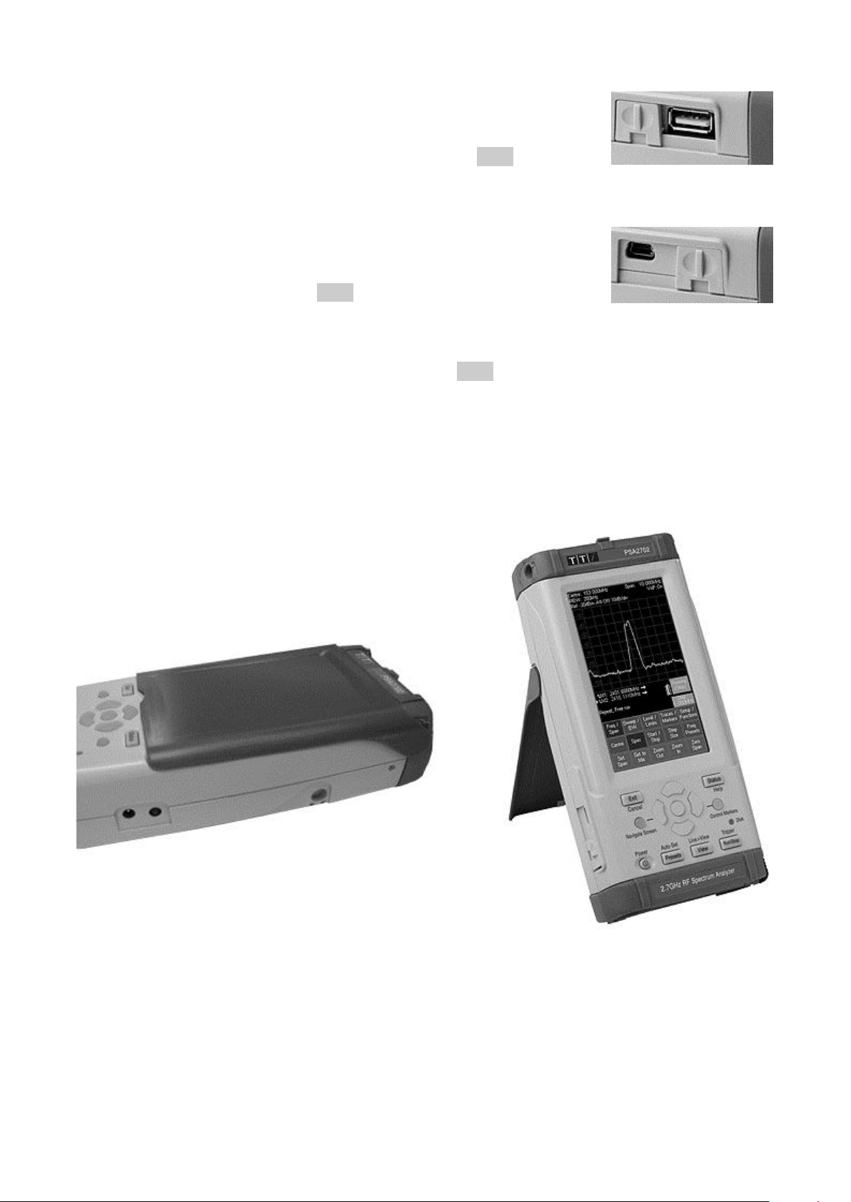
3.1.4 USB Host Connector (for USB Flash Memory)
A standard USB type A connector is provided on the left hand side of
the instrument which is revealed by moving the sliding cover towards
the top of the instrument. This is intended exclusively for the
connection of a USB Flash memory stick. See section 5.6.4 for full
information.
3.1.5 USB Device Connector (for connection to a PC)
A USB type mini-B connector is provided on the left hand side of the
instrument which is revealed by moving the sliding cover towards the
base of the instrument. This is intended exclusively for connection to a
personal computer. See section 5.6.5 for full information.
3.1.6 Trigger Input/Output
A 3.5mm mono jack socket is mounted at the top of the instrument for trigger signals. This has
no function unless option U01 is fitted - see section 6.1.2. An adaptor is provided that converts
from the jack socket to a standard BNC connector.
3.2 Bench-top and Portable Use
The instrument is intended for both hand-held and bench-top applications. It has rubber feet for
horizontal or vertical use, or can be angled using the tilt stand.
3.2.1 Tilt Stand
The instrument is supplied with the tilt stand folded
away and magnetically latched at the bottom of the
instrument. It can be hinged outwards to tilt the unit at
an angle of about 40 degrees.
3.2.2 Screen Protector and Sun Shield
To protect the screen when in transit, the tilt stand can
be detached from the bottom of the instrument and reattached on the top to act as a screen protector.
The stand is removed by flexing it outwards at the hinged end until the lugs disengage from the
sockets.
For outdoors use, the screen protector can be hinged upwards to form a sun shield which
improves the screen visibility in direct sun light.
When not required, it can be detached and stowed away on the back of the instrument where it
functions as a tilt stand .
Page 8
Page 10

3.3 Batteries and AC Line Power
3.3.1 Battery Operation
The instruments operates from an internal Lithium-ion rechargeable battery which can provide
more than 8 hours of continuous operation (screen brightness dependent).
The battery condition is indicated on the display via a multi-segment battery symbol. When it
changes colour to yellow, expected battery life has fallen below 1 hour. When it turns red,
expected battery life has fallen below 20 minutes.
The approximate battery life remaining is also displayed in hours and minutes within the Status
information screens.
The battery is charged from the supplied 5V/2A charger which can recharge a fully discharged
battery in under 3 hours.
When the battery is being charged, the red lamp next to the charging socket flashes. When
charging is complete, flashing ceases but the lamp remains illuminated while the charger is
connected.
It is also possible to slow charge the instrument from the USB port of a personal computer
provided that the instrument is turned off. Charge time may be up to 10 hours. Connection to
the PC must be made from the mini USB “device” port of the instrument using the supplied
cable. It is not possible to operate the instrument from USB power.
3.3.2 AC Line Operation
For bench-top operation, the instrument can be operated continuously from the supplied ac-line
operated charger. The internal power management circuitry ensures that the battery cannot be
overcharged.
3.3.3 Power Saving for Battery Operation
The battery life of the instrument is affected by the screen brightness which can be adjusted
over a wide range (see section 4.9.2). Setting the brightness to maximum, for example, will
reduce battery life by up to 2 hours relative to the normal setting (40%).
To conserve the battery the instrument should be turned off when not in use. In addition, AutoOff mode can be selected whereby the unit turns off automatically after a defined period from
the last key press. The period can be set between 5 and 60 minutes - see section 4.10.3.2.
Auto-Off is automatically disabled when external power is connected, and when data-logging is
enabled. All data is retained when the instrument is off.
Page 9
Page 11
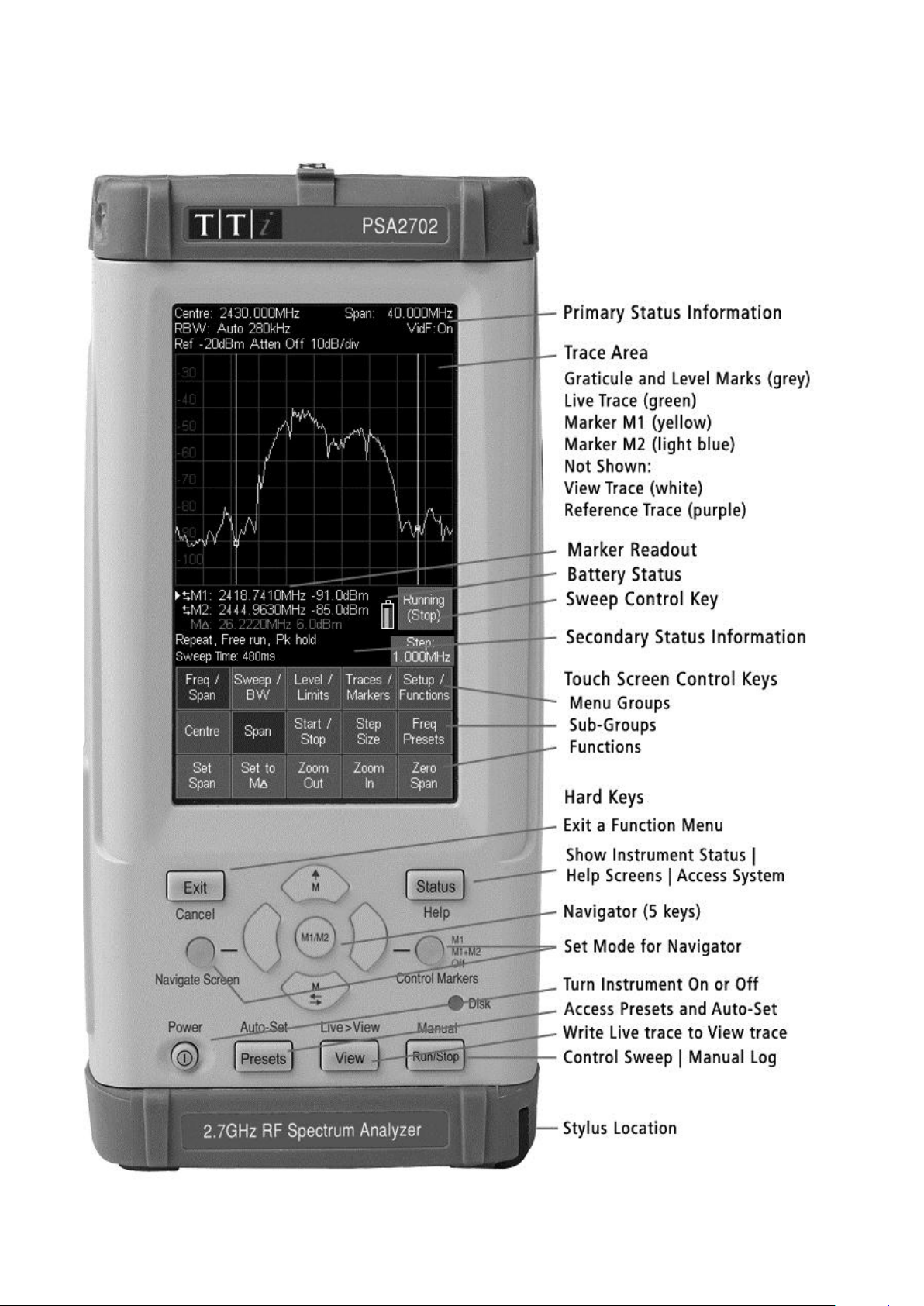
3.4 Display and Controls Layout
Fig. 1
Page 10
Page 12

3.5 Touch Screen Operation
The normal mode of operation of the spectrum analyzer is by using the touch-screen keys
within the display supplemented, when required, by the hard keys below.
The touch screen keys are normally operated by pressing with the finger or thumb, but can
alternatively be operated using the supplied stylus.
3.5.1 Finger Tip Operation
The touch screen is a resistive single-touch type (rather than the capacitive multi-touch type used
on many smart phones).
It can be operated by pressing the key area firmly with the soft part of the finger or thumb.
However, for greater positional accuracy it can also be operated by pressing gently with the finger
nail.
When the key is depressed, its colour changes from blue to purple. The key action is performed
when the key is released.
3.5.2 Stylus Operation
Some users may prefer to use a stylus to operate the touch screen. The supplied stylus has a
soft point. Sharply pointed objects should never be used to operate the screen as they could
cause damage.
The stylus should be replaced into its mounting slot at the base of the instrument to prevent it
being mislaid. The stylus design is compatible with those used with the Nintendo DS handheld
games console, and spares are widely available.
3.5.3 Operation using only the Hard Keys
It is also possible to use the spectrum analyzer without touching the screen at all, by using the
five “navigator” hard keys to operate each of the touch screen functions. See section 7.1 for a
full explanation of this mode of operation.
3.5.4 Navigator Keys - Mode Selection
The five hard keys that make up the Navigator have two alternative modes of operation which
are selected by the small illuminated keys on either side.
The modes are:
Control Markers - see section 4.7.2.1, and Navigate Screen - see section 7.1.
Whenever the navigator mode is changed, an information box appears explaining the current
action of the navigator keys. If preferred this can be turned off - see section 4.10.3.3.
3.6 Instrument Status Information
The most important elements of the instrument status are displayed at the top of the screen
(see Fig. 1 in section 3.4). Further status information relevant to the current menu function is
shown directly above the key area.
In addition, the full status of the instrument can be displayed at any time by pressing the hard
key marked Status/Help - see section 4.10.1.
3.7 On-screen Help
The instrument incorporates extensive help information to assist the user. Help is accessed by
pressing the hard key marked Status/Help - see section 4.10.2.
Page 11
Page 13
4 Operation using the Menu System
Freq/
Span
Sweep/
BW
Level/
Limits
Traces/
Markers
Setup/
Functions
Centre
Span
Start/
Stop
Step
Size
Freq
Presets
Freq/
Span
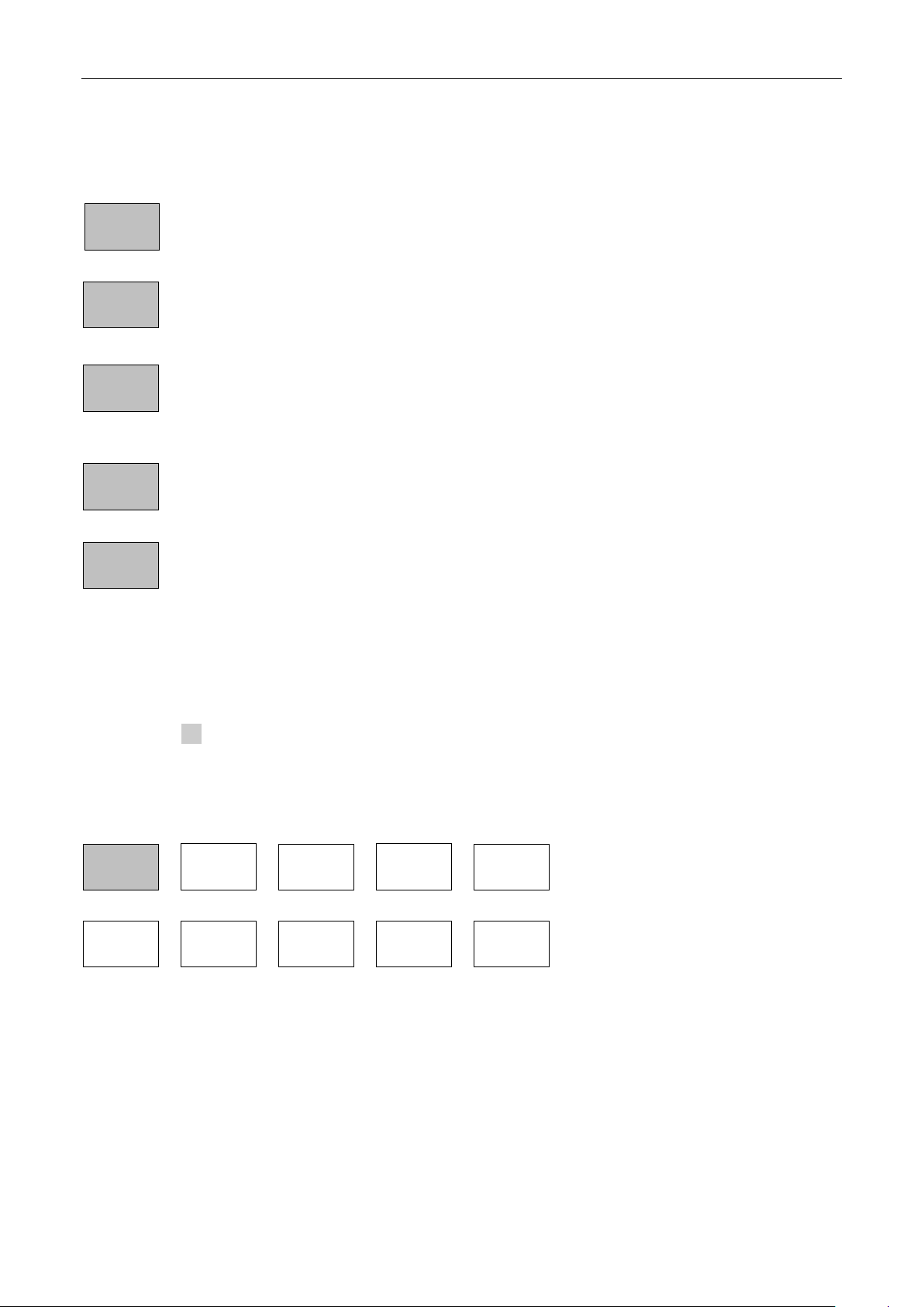
The default menu system for the spectrum analyzer consists of three rows of five keys. The
upper row represents the top level of the menu system and defines five “menu groups” as
follows:
enables the frequency range of sweep to be set in terms of start and stop
frequencies or centre frequency plus span.
enables the type of sweep to be set (repeat or single shot) and the resolution
bandwidth and video filter for the sweep to be selected. When option U01 is fitted, it
also enables sweep triggering.
enables the reference level to be changed, the amplitude units to be changed, and
the vertical scaling to be altered. When option U01 is fitted, it also enables the
setup and control of limit lines and patterns, and the application of external offsets
and compensation tables.
provides control of the display traces along with the storage function for both traces
and screen images. Also provides setup and control of the measurement markers.
provides access to the storage of instrument setups and system utilities. When
option U01 is fitted, it also provides access to automatic logging functions.
Each group has up to five “sub-groups” which appear on the middle row of keys. The currently
selected group and sub-group is shown by the relevant key being dark blue.
The bottom row of keys represent the “functions” that can be performed for each of the many
sub-groups. These keys may perform an immediate action, or bring up a pop-up menu, or
create a special control screen for numeric entry or file operations.
See section 15 for a graphical summary of the menu tree.
4.1 Setting the Frequency Range of the Sweep
This menu group controls the frequency range for the current sweep of the spectrum analyzer.
The range can be set in terms of either a centre frequency plus a span width, or in terms of a
start frequency and a stop frequency.
Pressing Centre or Span will cause the frequency range to be displayed at the top of the screen
in terms of a centre frequency and a span. Pressing Start/Stop will cause it to be displayed in
terms of a start frequency and a stop frequency.
The lowest start frequency is 1MHz. The highest stop frequency is 2700MHz or 1300MHz. The
minimum span width is 0.27MHz which results in minimum and maximum centre frequencies of
1.135MHz and 2699.865MHz or 1299.865MHz respectively.
Page 12
Page 14
4.1.1 Centre
Centre
Set
Centre
Set
C=M1
Set
C=Pk
Step
Down
Step
Up
Span
Set
Span
Set to
Mdelta
Zoom
Out
Zoom
In
Zero
Span
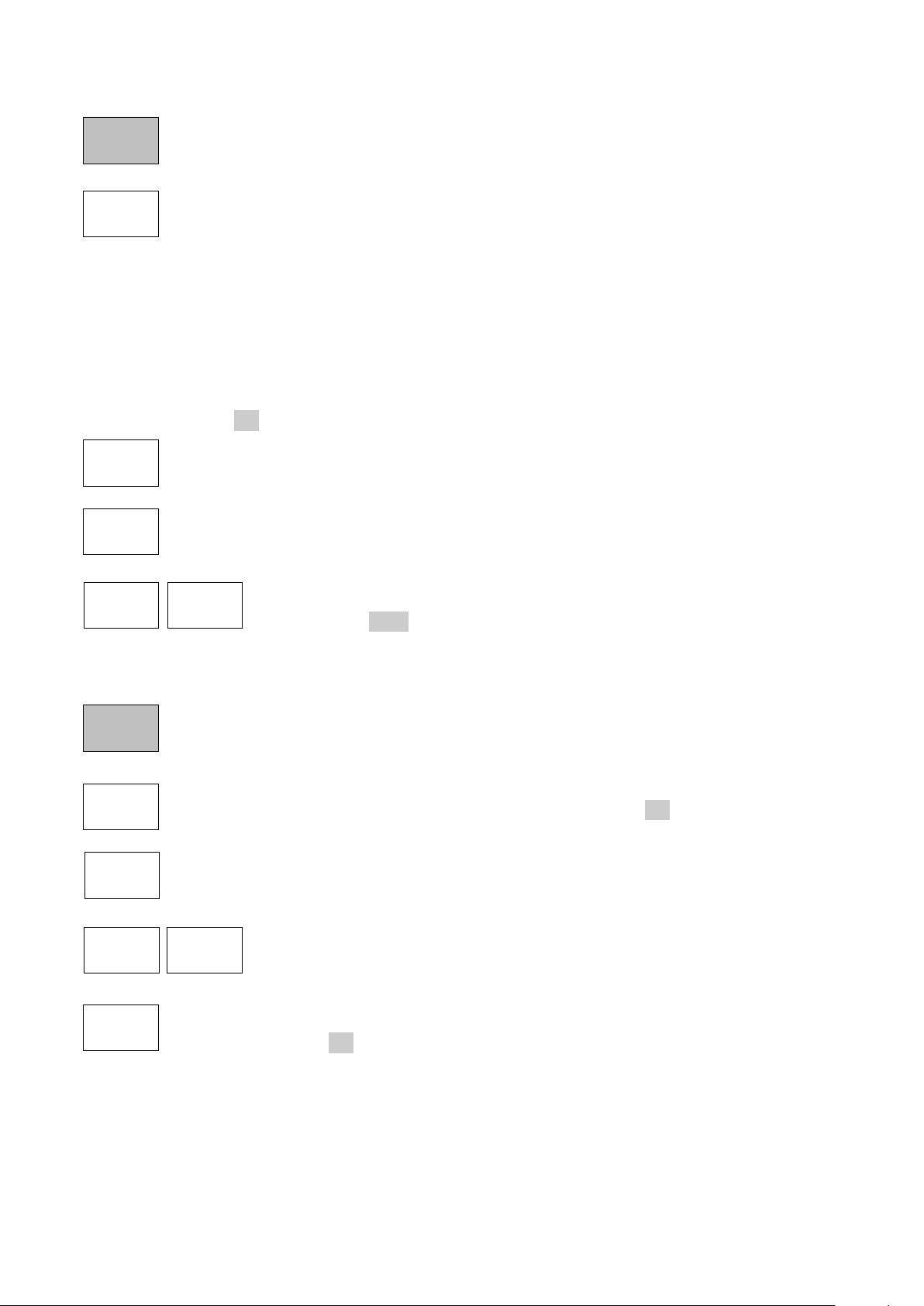
controls the centre frequency for the sweep. Also sets the annotation to
Centre/Span if it was previously Start/Stop. Creates a set of bottom-row function
keys as follows:
enables the centre frequency to be set to a specific value. The menu keys are
replaced by a numeric keyboard from which a centre frequency can be entered in
MHz to a resolution of 0.001.
Press OK to activate the new frequency without leaving the screen or OK & Exit to
return to the menu. Once a new frequency has been set from this screen, the
Previous key can be used to return to the previous frequency and then toggle
between the two.
Pressing Set by Tab/Jog selects an alternative setting screen in which frequencies
are set by “jogging” each digit up or down. Note that whichever method of setting
frequency is used becomes the default whenever Set Centre is pressed. See
section 7.2 for an illustrated description of frequency setting.
sets the centre frequency to the frequency value of the M1 marker (when active).
sets the centre frequency to the frequency value of the highest amplitude point in
the current sweep.
4.1.2 Span
controls the span for the sweep. Also sets the annotation to Centre/Span if it was
previously Start/Stop. Creates a set of bottom-row function keys as follows:
enables the span to be set to a specific value. The method for setting the span is
similar to that for setting the Centre frequency - see section 7.2 for an illustrated
description of frequency setting.
sets the span equal to the frequency difference between the M1 and M2 markers (if
active).
changes the sweep mode of the spectrum analyser and opens the Zero Span sub
menu - see section 4.3.
changes the centre frequency by the value of the step size
- see section 4.1.4.
sets the span to a higher or lower value in a 1-2-5 sequence starting from
the existing span value. (Example: if the existing span is 1.7MHz, the first
press of Zoom Out will take it to 2MHz and the next press to 5MHz).
Page 13
Page 15
4.1.3 Start/Stop
Start
Stop
Set
Start
Set
Stop
Start=M1
Stop=M2
-more1 of 2
Fix
Start
Fix
Stop
Step
Down
Step
Up
-more2 of 2
Step
Size
Auto
Span/10
Set to
Mdelta
Set to
Centre
Set to
M1
Set
Step
Undo
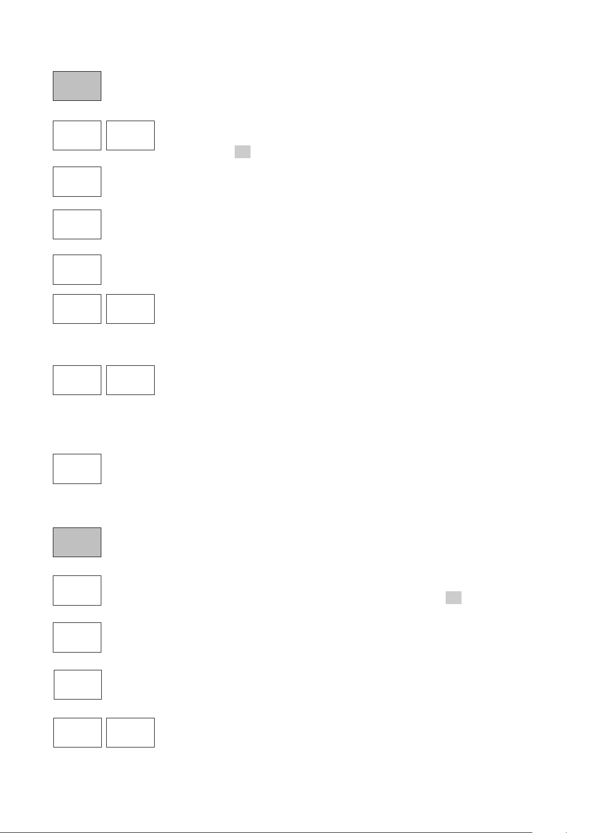
controls the start and stop frequencies for the sweep. Also sets the annotation to
Start/Stop if it was previously Centre/Span. Creates a set of bottom-row function
keys as follows:
enables the start or stop frequency to be set to a specific value. The
method for setting these is similar to that for setting the Centre frequency
- see section 7.2 for an illustrated description of frequency setting.
sets the start frequency to the frequency of the M1 marker and the stop frequency to
the frequency of the M2 marker. M1 and M2 must both be active and M2 must be at
a higher frequency than M1.
reverts to the start and stop frequencies that existed directly before the
Start=M1/Stop=M2 key was pressed.
opens a second set of actions keys: Fix Start/Fix Stop and Step Down/Step Up.
changes the action of the Step Up/Down keys so that only the stop
frequency or start frequency respectively is changed by the step value.
The fixed start or stop frequency is preceded by the word Fix. Pressing
the key again, or leaving this function-set (by pressing -more- 2 of 2 or any group or sub-group
key) will cancel the fixed start or stop frequency.
changes the start and/or stop frequencies by the value of the step size
(see next section). The action of the Fix Start/Fix Stop keys determines
whether both are stepped or only one is stepped.
Note that, if the start or stop frequency is “fixed” and the step size is set to Auto, the step size
will change on each press of step up/down so that it is always equal to one graticule division.
returns to the alternative set of action keys for Start-Stop. Cancels the fixed start or
stop frequency if set.
4.1.4 Step Size
sets the size of frequency stepping using the Step Up/Down keys. When relevant,
the current step size is displayed within a green box above the keys. Creates a set
of bottom-row function keys as follows:
enables the step size to be set to a specific value. The method for setting the step
size is similar to that for setting the Centre frequency - see section 7.1 for an
illustrated description of frequency setting.
causes the step size to be automatically linked to the width of the span. Thus
Step/Up down will cause the centre frequency to change in steps of one graticule
division. Auto step size is indicated by the word Auto above the step size value.
sets the step size equal to the frequency difference between the M1 and M2
markers (if active).
sets the step size equal to either the centre frequency or to the frequency
of the M1 marker (if active). This can be useful for observing the
harmonics of a fundamental frequency.
Page 14
Page 16
4.1.5 Frequency Presets
Freq
Presets
Full
Span
Recall
Preset
Toggle
Last
Exit
Z-Span
Demod
Volume
-
Volume
+
Store
Preset
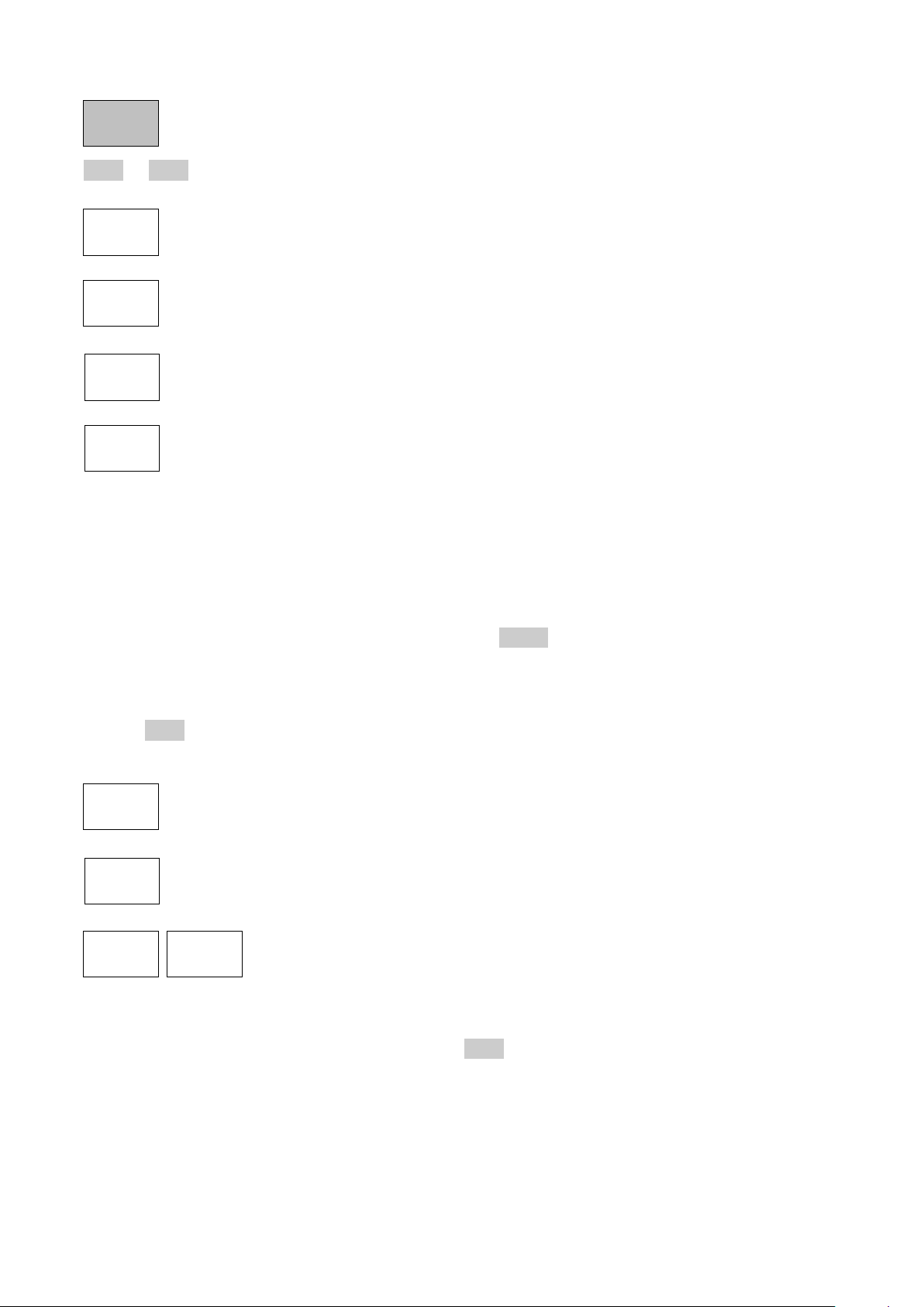
enables up to six frequency ranges to be quickly stored and recalled. Only the
centre and span (or equivalent start and stop frequencies) are stored. This differs
from a Trace State or Set-up file for which more parameters are stored (see sections
5.7.1 or 5.7.3 respectively). Frequency presets are retained when the instrument is off.
Creates a set of bottom-row function keys as follows:
sets the sweep to the full range of the instrument (1MHz to 2.7GHz or 1.3GHz).
brings up a menu of six preset numbers (1 to 6) into which the current value of the
sweep frequency range can be stored. Existing values are over-written.
brings up a menu of six preset numbers (1 to 6) which recall previously stored
frequency ranges. Empty positions are ignored.
switches between the current sweep frequency range and the last range to be
recalled from a preset (or from Full Span).
4.2 Sweep Time
The sweep time and update rate is automatically set from the Span and the RBW and is
displayed within the lower annotation area. There is no independent adjustment of sweep time.
Narrower RBW settings create longer sweep times. For each RBW, the sweep time in broadly
proportional to the frequency span. The approximate formula for calculating sweep update
times is given within the specifications – see section 12.1.4.
4.3 Zero Span Mode
Zero span is a special case of frequency range setting. It is set from the Span sub-menu - see
section 4.1.2. Pressing Zero Span changes the trace display to be a horizontal line at the
centre frequency amplitude level, and brings up an alternative set of function keys as follows:
exits zero span mode and returns to a normal swept trace and the normal Span submenu key functions.
brings up a menu which enables the demodulation mode to be set to AM or FM (or
Off) and the Audio Filter to be set to On or Off.
adjusts the demodulated audio volume (0 to15). The value shown on a
grey bar graph.
The demodulated audio is routed to a built-in loudspeaker. Alternatively, the audio can be
outputted via a 3.5mm jack socket - see section 3.1.3.
Page 15
Page 17
4.4 Setting the Sweep Mode and Sweep Bandwidth (RBW)
RBW
Video
Filter
Sweep
Sweep/
BW
RBW
Auto
15kHz
280kHz
1MHz
Video
Filter
On
Off
Sweep
Repeat
Single
Sweep
Trigger
This menu group controls the sweep and the resolution bandwidth.
This enables the sweep to be controlled in terms of the type of sweep (repeat or single) and the
resolution bandwidth of the sweep filter and the subsequent video filtering. If option U01 is
fitted, sweep triggering can also be controlled.
4.4.1 RBW
controls the resolution bandwidth of the sweep filter. A narrower RBW provides
greater frequency resolution and lower noise, but increases the sweep time.
Creates a set of bottom-row function keys as follows:
causes the RBW to be automatically changed to suit the frequency span. The RBW
value is displayed at the top of the screen and is preceded by the word Auto.
4.4.2 Video Filter
controls the video filter. With the video filter On, displayed noise levels are lower,
but signals may be slightly attenuated at narrower RBW settings. Creates a set of
bottom-row function keys as follows:
4.4.3 Sweep
controls how and when the sweep runs. Creates a set of bottom-row function keys
as follows:
causes the sweep to be automatically restarted after the completion of the previous
sweep unless halted by the Sweep Control key (or the Sweep Trigger settings).
enables single sweeps that are commenced by the Sweep Control key (or the
Sweep Trigger settings).
manually selects a specific RBW value which is displayed at
the top of the screen
The status of the video filter is shown at the top of the screen preceded
by the word VidF .
Note that, whenever the sweep is stopped, whether in repeat or single mode, changing the
frequency span or the reference level will re-run the sweep once.
Sweep Trigger is only available with the upgrade option U01 is fitted. It provides a
choice of how the sweep is started or stopped. The trigger source can be manual,
external, or internal from limit lines or patterns. See section 4.4.3.3 for an
explanation of trigger functions.
Page 16
Page 18
provides a choice of automatic or manual re-arming of the trigger when triggering is
Single
ReArm
Stopped
(Run)
Running
(Stop)
Stopped
(Single)
enabled and the sweep mode is set to Single.
When the menu system is set to Sweep/BW > Sweep the sweep status is displayed in the lower
annotation area directly above the keys.
4.4.3.1 Sweep Rate and the Sweep Progress Indicator Line
The sweep time and resultant update rate is a function of the span and the RBW and is shown
within the lower annotation area. It can be calculated from the formulae within section 12.1.4.
For sweep times slower than about 1 second, a yellow indicator line below the graticule
indicates the progress of the sweep – see section 4.6.2.
4.4.3.2 Manually Controlling the Sweep
The sweep can be started or stopped using the touch screen Sweep Control key
directly under the graticule on the right hand side. This key changes colour to
indicate the current state of the sweep. The action of the key is duplicated by the
hard key marked Run/Stop.
When the sweep is running, the key is green and is marked Running (Stop). The word in
brackets indicates the action that will be performed by pressing the key.
When the sweep is stopped, and the sweep mode is Repeat, the key is blue and is
marked Stopped (Run). Stopping the sweep freezes the current sweep trace on the
display so that it can be observed.
When the sweep is stopped, and the sweep mode is Single, the key is blue and is
marked Stopped (Single).
At other times, when the sweep is temporarily halted by the system, the key
becomes red and is marked Paused. When sweep triggering is enabled (see next section) the
key can provide triggering and arming functions which are indicated by other colours and
markings.
4.4.3.3 Triggered Sweep (when fitted)
When upgrade option U01 is fitted, it is possible to trigger the sweep using an external or
internal trigger signal. Triggered sweep has a different action dependent upon the sweep mode
(Single or Repeat).
If the sweep mode is set to Single, the effect of the trigger is to start the sweep. When a trigger
event occurs a single sweep will be initiated. The trigger options are None, Ext +ve (trigger
from a positive going edge on the external trigger input) or Ext -ve.
If Single ReArm is set to Auto, a sweep will be initiated every time a trigger event occurs. If
Single ReArm is set to Manual, further trigger inputs are ignored after the first sweep. The
Sweep Control key turns yellow and is labelled Stopped (Arm). Pressing the key changes the
labelling to Run on Trigger, and a further sweep will be initiated as soon as a trigger event
occurs.
If the sweep mode is set to Repeat, the effect of the trigger is to stop the sweep. The options
are Free Run (no triggering), Ext +ve (trigger from a positive going edge on the external trigger
input), Ext -ve, and Limits (trigger from the Limits comparator - see section 7.6.2). The key
marking becomes Stop on Trigger.
When a trigger occurs the current sweep will be completed after which the sweep control key
will become blue and the sweep will remain stopped until it is restarted with the sweep control
key. There is no separate Arming function for repeat mode sweeps.
Sweep triggering is turned off whenever the sweep mode is changed between Single and
Repeat or vice versa.
Note that, when a Logging file is initiated, triggered sweep is automatically cancelled and set to
Repeat mode and Free Run.
Page 17
Page 19
4.5 Setting the Level Attenuator, Amplitude Scale, and Limits
Units/
Graticule
Ref
Level
Scale/
Shift
Offset/
Tables
Limits
Level/
Limits
Ref
Level
0dBm
-20dBm
Scale/
Shift
Scale
Shift
Down
Shift
Down
Units/
Graticule
dBm
dBuV
Graticule
This menu group controls the input attenuator, thus changing the reference level, and controls
the measurement units and scaling of the amplitude display. When option U01 is fitted, it also
enables the sweep amplitude to be compared with limit lines or patterns and the use of level
offset and compensation tables.
4.5.1 Measurement Units and Graticule
sets the measurement units and controls the graticule display. Creates a set of
bottom-row function keys as follows:
provides measurement in dBm (dB milliwatts into 50 Ohms, where 0dBm = 1mW)
and sets the graticule and graticule markings accordingly.
provides measurement in dBuV (dB micro volts across 50 Ohms, where 0dBuV =
1uV) and sets the graticule and graticule markings accordingly.
creates a pop-up menu enabling the Graticule to be dimmed, set to show levels
only, or turned off completely.
4.5.2 Reference Level
the reference level for amplitude measurement is changed by switching the
attenuator On or Off. Creates a set of bottom-row function keys as follows:
sets the reference level to 0dBm (or 107dBuV) by setting the attenuator to On. The
setting is shown within the upper area of the screen.
sets the reference level to -20dBm (or 87dBuV) by setting the attenuator to Off. The
setting is shown within the upper area of the screen.
4.5.3 Vertical Scaling
enables the vertical amplitude scaling to be changed. Creates a set of bottom-row
function keys as follows:
creates a pop-up menu enabling the vertical scaling to be set to 10dB/div (the
default) through to 1dB/div.
For scales below 10dB/div only a portion of the sweep amplitude will be
visible and the Shift Up/Shift down keys can be used to pan the trace
through the amplitude range of the graticule. These keys auto-repeat.
Page 18
Page 20
4.5.4 Amplitude Offset and Compensation Tables (when fitted)
Offset/
Tables
Clear
All
Set
Limits
Limit
Conditio
Limit
Action
Set
Limits
Limit
Condition
Limit
Action
Limit
Offset
Limit
Fix/Unfix
enables the amplitude scaling to be offset to match external attenuation or gain, or
to add frequency dependent amplitude compensation tables to match transducers or
antennae. These functions are only available when the upgrade option U01 is fitted
- see section 6. Creates a set of bottom-row function keys as follows:
cancels any offset or compensations that have been set and returns the amplitude
scaling to normal.
opens a control menu that enables compensation for a 75 Ohm source impedance,
a fixed attenuation or gain, or a frequency dependent compensation table to be
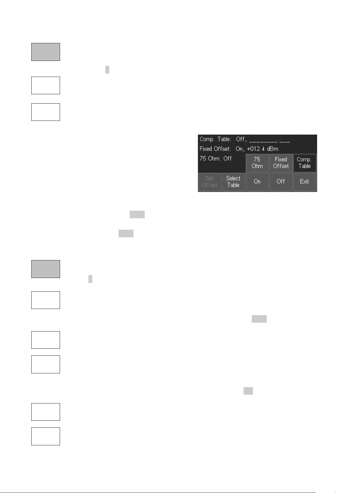
used. The functions can be used individually or together.
The three keys on the upper line select which function
is to be controlled.
For 75 Ohm source, the options are only on or off.
For Fixed Offset, the Set Offset key creates a
dialogue box by which an offset can be set between
-50.0dB and +50.0dB. The set figure is added to the
displayed reference level and to the graticule values
and marker readout.
For Compensation Table, the Select Table key opens a file list of stored compensation tables
that can be loaded. See section 7.5.2 for a full explanation.
Whenever offsets or compensations are active, a warning message is displayed at the top right
of the graticule. See section 7.5.1 for safety warnings on the use of these function.
4.5.5 Amplitude Limits (when fitted)
sets one or two horizontal lines or a complex patterns that can be compared with the
sweep. This function is only available when the upgrade option U01 is fitted - see
section 6. Creates a set of bottom-row function keys as follows:
creates a control screen that enables the selection of lines and patterns, or allows
existing ones to be turned on or off. When Set Line is pressed, the value can be
entered numerically in dBm or dBuV. When Select Pattern is pressed, a Recall File
screen is opened enabling a pattern to be loaded from a file. See section 7.6.1.
creates a pop-up menu that selects the criteria upon which a limit condition is
created. The options are None, Above, Below, Outside or Inside.
creates a pop-up menu that selects an action that will be performed when the limit
condition occurs. The options are None, Beep, Pulse Out, Beep + Pulse Out or
Message (Pass/Fail).
Note that other actions (sweep triggering or log file entry) can also be created from the limits
condition. Further information on the Limits function is given in section 7.6.
creates a control screen from which a limit can be offset from its initial values. This
is particularly useful for limit patterns which would otherwise have to be recreated.
allows a limit pattern, once loaded, to be fixed relative to the screen enabling it to be
used for any centre frequency rather than just the one for which it was created.
Page 19
Page 21
4.6 Controlling and Storing Traces and Images
Traces
Control
Trace
Mode
Traces
Stores
Marker
Setup
Marker
Control
Traces/
Markers
Traces
Control
Show
Traces
View
Swap
View
Off/On
This menu group controls the traces that appear on the screen (as well as the markers that are
used for measurement).
There are three traces: Live (green), View (white) and Reference (purple). Only the Live trace
is updated from the sweep. The View trace is a temporary copy of the live trace created
whenever the View key is pressed. The reference trace is recalled from a trace file stored
within the instrument. Trace files can be saved from either the live trace or the view trace.
Complete images of the screen can also be saved.
4.6.1 Displaying Traces; Controlling the View Trace
enables each of the three trace types to be turned on or off, controls the View trace,
and enables traces and screen images to be stored and recalled. Creates a set of
bottom-row function keys as follows:
enables each of the three trace types to be turned on or off via a pop-up menu.
copies the current Live trace to the View trace, and turns the View trace on if it was
off. The View trace sits behind the live trace and can therefore be partly obscured
by it .
toggles the View trace off, or back on without creating a new View (this is a shortcut
to the function provided by the pop-up menu on the Show Traces key).
halts the live trace and swaps the order of the traces on the screen. Thus the View
trace (white) sits in front of the halted live trace enabling it to be observed and
analyzed using the markers. When the sweep is restarted with the Sweep Control
key, the traces are swapped back so that the Live trace sits in front again.
4.6.1.1 Understanding the Live, View and Reference Traces
The instrument can display three traces - Live, View and Reference which can be turned on or
off individually using the Show key. Only the Live trace is updated from the sweep.
The Live trace is green and is normally on-top of the other traces. The Live trace can be
“frozen” at any time by pressing the Sweep Control key directly under the graticule (see section
3.4) or the hard key marked Run/Stop. This also stops the sweep.
The Live trace can be duplicated to the View trace by pressing View. This enables an
“instance” of the sweep to be captured without stopping the sweep. The View trace is white
and is normally located behind the Live trace. The View trace is retained when the instrument
is turned off.
The measurement markers normally operate on the Live trace. However, the Live and View
traces can be “swapped” by pressing the Swap key. This stops the sweep and causes the View
trace to be placed in front of the Live trace. When the traces are swapped, the measurement
markers operate on the View trace.
Page 20
Page 22
When the sweep is re-started (or the Swap key pressed again), the View and Live traces are
Trace
Mode
Normal
Average
Number
Reset
Traces
Stores
Store
Recall
Peak
Hold
Average
swapped back.
Either the Live trace or the View trace can be saved to a trace file (see section 5.1).
The Reference trace is purple and is always underneath the other traces if they are on. The
reference trace is created by recalling a trace file from the memory. Measurement markers
cannot be used on a Reference trace.
Note that the View and Reference traces relate to the frequency span, RBW and level settings
that existed when they were stored. Changing these parameters will result in the graticule
values and annotations no longer being correct for these traces.
However, it is possible to recall a Reference trace along with its State. This restores the
frequency span, RBW and level settings that existed when it was stored (see section 5.1).
4.6.2 Sweep Progress Indicator Line
There are two modes by which the live trace is updated from the sweep. For sweep times
below approximately 1 second, the trace is updated at the end of the sweep. For longer sweep
times, the trace is updated continuously while the sweep is taking place.
In this latter mode a yellow line appears at the bottom of the graticule indicating the progress of
the sweep through its span.
4.6.3 Setting the Trace Writing Mode
provides control of the way in which the sweep is written to the Live trace. Creates
a set of bottom-row function keys as follows:
each frequency point of the trace is written with the amplitude obtained from the
current sweep.
the trace is written with the highest amplitude value found for each frequency point
since sweeping was commenced.
the trace is written with the average amplitude value over a number of sweeps..
creates a pop-up menu that enables the number of sweeps averaged to be set
between 2 and 48 .
operates in both Average and Peak hold modes and re-starts the averaging or peak
hold process from zero.
4.6.4 Storing and Recalling Traces and Screen Images
Traces or complete Screen Images can be stored as files under automatically
incrementing names or user assigned names. Creates a set of bottom-row function
keys as follows:
enables the Live trace, the View trace, or a complete screen image, to be saved as
a file. See section 5.1 for a full description of the Store function.
enables a stored trace to be recalled to the Reference trace on the screen. The Ref
trace is purple and is always behind both the Live trace and the View trace. Recall
also enables stored screen images to be viewed. See section 5.2 for a full
description of the Recall function.
Page 21
Page 23
4.7 Using Measurement Markers
Marker
Setup
Function
Fix /
Unfix M1
Move M2
to M1
Units
Select
Traces/
Markers
Traces
Control
Trace
Mode
Trace
Stores
Marker
Setup
Marker
Control
This menu group controls the markers that are used for measurement (as well as the traces
that appear on the screen).
There are two markers M1 and M2 which provide a readout of amplitude at any frequency point
on the trace. M2 can only be on if M1 is on, and the frequency difference between the two is
also shown. Markers can be set to automatically find peaks, or track the largest peak.
4.7.1 Setting-up Markers
controls the visibility of the markers, their function, and their measurement units.
Creates a set of bottom-row function keys as follows:
creates a pop-up menu that enables the markers, M1 and M2, the be turned on or
off. Note that M2 can only be on if M1 is also on.
creates a pop-up menu that enables the marker measurement units to be set.
Graticule Units provides logarithmic measurements in dBm or dBuV (as set within
the Level/Limits > Units/Graticule menu). uW (micro watts) or mV (millivolts)
changes the marker measurement to the appropriate linear scaling.
creates a pop-up menu with a choice of Scroll, Peak Find, or Peak Track modes. In
Scroll mode a single press of the Move Left/Right keys cause the selected marker to
move in one pixel steps (i.e. a frequency step of span/270), whilst holding a key
down auto-repeats in larger steps.
In Peak Find mode the Move Left/Right keys cause the selected marker to jump to the next
peak of the trace in that direction. In Peak Track mode, the marker will attempt to maintain its
position on the highest peak of the trace even when the peak frequency is changing (see
section 4.7.2.2 for a fuller explanation of Peak Find/Track modes).
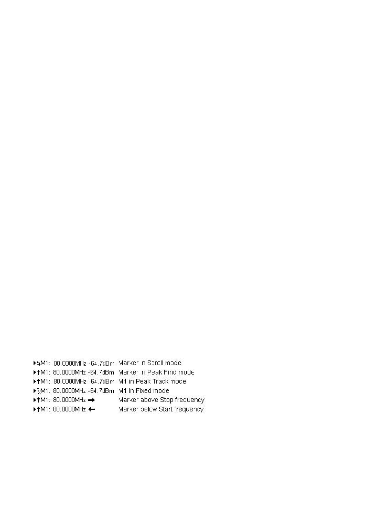
The current mode of a marker is shown on the left hand side of the marker read out. Two
horizontal arrows indicate scroll mode whereas an upwards vertical arrow indicates peak-find
mode. An upward arrow followed by a small T indicates peak-track mode.
fixes the amplitude reading of the M1 marker so that it no longer follows level
changes from the sweep. The marker readout is preceded with the word “Fix”.
Pressing the key again, or pressing either of the marker “move” keys, returns M1 to
normal operation.
moves the M2 marker to the frequency position of the M1 marker (also turns M2 on
if it was off). This is intended for use with the Fix M1 function to enable amplitude
changes at a specific frequency to be monitored.
Page 22
Page 24
4.7.2 Controlling Markers
Marker
Control
Move
Left
M1/M2
Active
Move
Right
Marker
>Centre
Manual
Set
controls the frequency position of the markers. Creates a set of bottom-row function
keys as follows:
selects which marker is controlled by the marker movement keys. The active
marker is indicated by an arrow (>) in front of its readout.
enables the frequency position of the active marker to be set numerically using
similar frequency entry screens as for Set Centre (see section 4.1.1). Note that the
marker position can be set outside of the current span and therefore off the screen.
moves the active marker to the sweep centre frequency (i.e. the centre of the trace).
This is particularly useful if the active marker is off the screen.
moves the active marker left or right either in frequency steps or from
peak to peak of the trace depending on the Marker Mode (Scroll or Peak
Find). In Scroll mode, a single press moves one pixel on the display and
holding the key down causes it to move continuously in steps of about ten pixels.
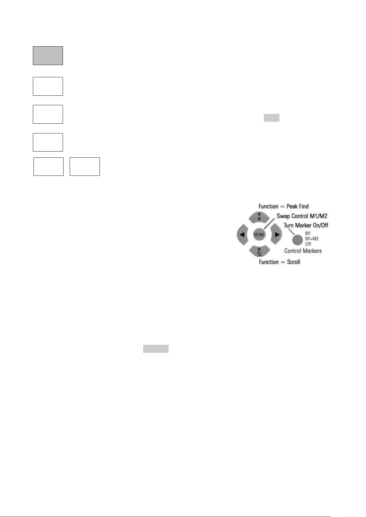
4.7.2.1 Controlling Markers with the Hard Keys
The normal function of the five “navigator” hard keys in the
centre of the instrument is to control the markers. This allows
control at all times without the need to select the Marker Setup
or Marker Control sub-group menus.
When the navigator keys are in this mode, the round key
marked Control Markers is illuminated. If not, pressing the
key will restore this mode. Pressing the key repeatedly cycles
through selection of the visible markers (Both Off > M1 Only >
M1 and M2 > Both Off).
Pressing the centre button on the navigator toggles the active marker between M1 and M2, or
turns M2 on if it is off. Pressing the Up key selects Peak Find function, while pressing the Down
key select Scroll function. Whenever the Up key is pressed, the selected marker will jump to
the highest peak.
The Left and Right keys move the active marker left or right either in screen resolution steps or
from peak to peak of the trace depending on the function.
Whenever the navigator mode is changed, an information box appears. This alert can be
turned off if preferred - see section 4.10.3.3.
4.7.2.2 Further Notes on the Use of Markers
Function = Peak Find
Peak Find mode is selected from Marker Setup > Function or from the Navigate Up hard key,
and is indicated by an upwards arrow on the left hand side of the marker readout. The mode is
selected for the marker that is currently active.
Pressing the Navigate Up hard key places the currently selected marker on the largest peak of
the trace.
Pressing the Move Left/Right keys will cause the instrument to attempt to position the marker
on the next peak of the trace in that direction. The peak-find algorithm may sometimes place
the marker on the rising or falling edge of a peak and its performance will depend upon signal
and noise levels.
Page 23
Page 25
Function = Scroll
Scroll mode is selected from Marker Setup > Function or from the Navigate Down hard key, and
is indicated by two horizontal arrows on the left hand side of the marker readout. The mode is
selected for the marker that is currently active.
Function = Peak Track
Peak Track mode can only be selected for M1. It is selected from Marker Setup > Function, and
is indicated by an upwards arrow followed by a capital T on the left hand side of the marker
readout.
When selected the marker will attempt to track the highest peak of the live trace.
Marker Frequency Precision
The frequency position of a marker is always shown to a resolution of 0.001MHz (1kHz).
However, the actual position of the marker is a function of the span. If, for example, the span is
set to 50MHz, each frequency point on the trace represents a “bucket” of frequencies 185kHz
wide (span/270).
If the marker is set using the Move Left/Right keys, it will give a frequency readout equal to the
upper frequency of the bucket. If the marker is set numerically to a specific frequency using
Manual Set, the marker position on screen will jump to the upper frequency of the bucket that
contains that numerical value.
If the span is reduced, the accuracy of the marker frequency readout improves. However, it is
only when the span is reduced to 270kHz that the marker frequency position becomes accurate
to 1kHz.
“Off Screen” Markers
Markers are positioned by absolute frequency. Consequently, when the frequency span of the
sweep is changed, the marker may no longer appear within the trace area. This is indicated by
an arrow within the marker readout replacing the amplitude value.
The frequency position of the marker is retained, but no amplitude information is available. If
the frequency span is subsequently changed to include the marker frequency, it will reappear in
the correct position.
Pressing the Navigate Up hard key (Peak Find mode) will bring the marker on screen at the
highest level in the trace.
Re-positioning a marker using the Move Left/Right keys will cause it to reappear immediately
from the appropriate side of the graticule. Alternatively pressing Marker>Centre in the Marker
Control sub-group menu will cause it to appear in the centre of the screen.
Marker Mode Symbols
Marker Difference Readout
If both markers are turned on, the difference in frequency and level is shown in grey underneath
as Mdelta. The readout represents the M2 values minus the M1 values (M2 - M1).
Page 24
Page 26
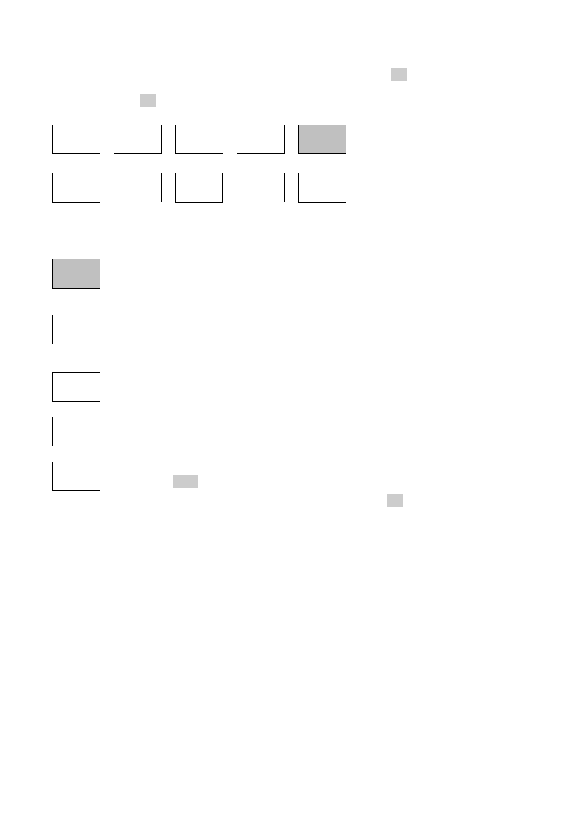
4.8 Data Logging Functions (when fitted)
Logging
Setups
System/
File Ops
Setup/
Functions
Logging
Timer
Setup
Log
Type
Log
Trigger
Logging
Control
This menu group controls logging functions when fitted (see section 6.1). It also controls
store/recall of instrument set-ups and access to system functions, which are covered in the next
section - section 4.9.
4.8.1 Setting-up the Logging Function
Logging is only available when the upgrade option U01 is fitted. Logging enables
files containing multiple traces, screen images or peak values to be created in
response to trigger events or a timer. Creates a set of bottom-row function keys as
follows:
creates a pop-up menu that enables the type of log file to be selected. Centre
Amplitude logs only the amplitude at the centre frequency. Peak Value logs the
frequency and amplitude of the highest peak in every sweep. Trace logs the whole
trace. Screen Image logs the whole screen as a bit-map image.
creates a pop-up menu that enables selection of the trigger event that will cause
each logging entry. The options are Manual, Timer, Ext +ve, Ext -ve, Limits and
Continuous.
enables the time interval between logging events to be set. The timer value is only
used when the log trigger is set to Timer.
opens a new control menu from which the logging function to be controlled
(see section 7.7.1).
For a more detailed description of the Logging function see section 7.7 .
Page 25
Page 27
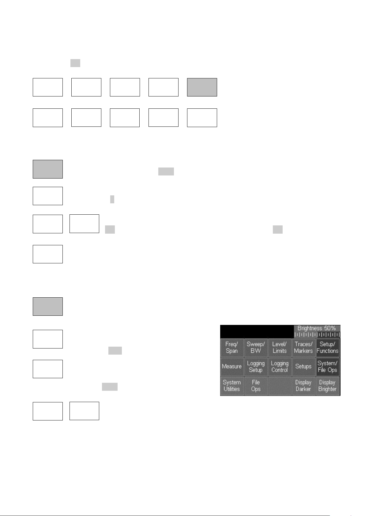
4.9 Storing and Recalling Set-ups | System Settings
Logging
Setups
System/
File Ops
Setup/
Functions
Setups
Store
Setup
Recall
Setup
Load
Defaults
System/
File Ops
Display
Darker
Display
Brighter
System
Utilities
File Ops
Presets
This menu group controls storing and recalling complete instrument set-ups, and access to
system functions such as screen brightness and file operations (as well logging when fitted see section 4.8).
4.9.1 Storing and Recalling Instrument Setups
enables the complete setup of the instrument to be stored and recalled via user
nameable files. See section 5.7.3 for an explanation of setup files. Creates a set of
bottom-row function keys as follows:
opens the Presets menu, duplicating the action of the PRESET hard key
(see section 0).
opens the store and recall control screens for setup files. See sections
5.3 for a description of the store screens, and section 5.4 for a
description of the recall screen.
loads the factory default setup, thus restoring the instrument status to its original ex-
factory settings. Note that no user-created files are modified or deleted.
4.9.2 System Settings, Screen Brightness, Filing System and USB Operations
provides access to some system and file management options, including screen
brightness and file transfer via USB. Creates a set of bottom-row function keys as
follows:
opens the System Utilities special menu, which
is also available via the Status/Help hard key
(see section 4.10)
enables file management in terms of
renaming, deleting and copying of files to or
from a Flash Memory Drive or a PC using the
USB link (see section 5.6.2).
changes the screen brightness and provides a bar graph showing the
current brightness level.
Page 26
Page 28
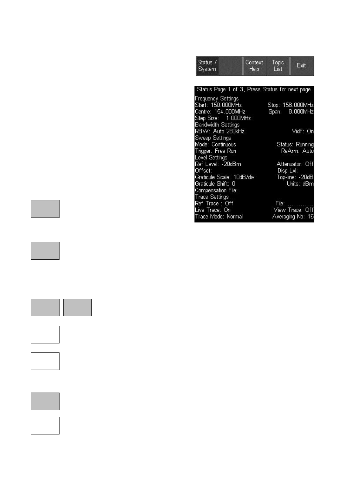
4.10 Status Information | On-screen Help | System Utilities
Context
Help
System
Utilities
Calibrate
Screen
Screen
Topics
List
Status/
System
Navig.
Help
System
Help
This menu group is accessed using the hard key marked STATUS/Help or by the soft key
Setup/Functions > System/File-Ops > System Utilities. When the key is pressed, the normal
key menu is replaced by a special menu as shown
opposite.
4.10.1 Status Display
When the Status/System key is selected, the top part
of the screen is replaced by a detailed listing of the
current instrument setup conditions.
The status information is split over three pages.
Press Status again to access the next page or press
Exit to return to normal operation and restore the
menu group and sub-group that were in place when
the Status hard key was pressed.
4.10.2 Help Screens
Help information is available from the same menu
system as is status, by pressing the Context Help or
Topic List keys.
brings up a help screen relevant to the
menu sub-group that was in use prior to
the Status/Help key being pressed.
Context Help may cover several pages, these are
selected with the Next/Prev Page keys.
brings up a topics list from which all of the individual help screens can be selected.
Select the required menu sub-group using Move Up/Down and confirm with Select
Topic.
Pressing Exit when displaying a Help screen returns the analyzer to normal operation.
4.10.3 System Utilities
Pressing Setup/Functions > System/File-Ops > System Utilities, or the
Status hard key followed by Status/System brings up a sub-group menu
as shown below:
opens an information window that shows the current settings of the five-way
navigator and explains how to turn navigator mode messages on or off.
opens a special Help screen relevant to the System Utilities functions. These are
not covered within the normal help topics.
4.10.3.1 Screen Utilities
enables aspects of the TFT color screen to be adjusted. Creates a set of bottom-
row function keys as follows:
opens a calibration screen for the touch screen. (The touch screen is a resistive
layer which overlays the TFT screen. From time to time it may be necessary to re-
calibrate the positional accuracy of the system).
Page 27
Page 29
Calibration must be done using a stylus, and the centre of the “bulls eye” must be touched
Pwr-On
State
Auto
Off
Power/
Clock
Set Date
& Time
Alerts
System
Update
Update
Firmware
Navig.
Prompt
Calibrate
Hardware
Install
Options
Beep
View
On PC
Bright
Level**
Navig.
Help
accurately in each of three positions. To abort the calibration, press the Exit hard key.
opens an information box explaining where the screen brightness controls are
located (Setup/Functions > System/File Ops). This is because screen brightness
should be adjusted with the trace and graticule displayed rather than the status
screen.
View on PC is only available with the upgrade option U01 is fitted. It places the
instrument into a special mode in which the graphics of the display are sent to a PC
via USB. See section 13 (Appendix A).
4.10.3.2 Power Options, Power-on State, Clock Setting
enables aspects of the power on-off system to be set, along with the real-time clock.
Creates a set of bottom-row function keys as follows:
opens a dialogue box from which the date and time can be set for the real-time
clock. Times are in 24 hour format and dates are day-month-year.
creates a pop-up menu that enables the instrument to be automatically turned off
after a period of inactivity. Options are Never and 5 mins to 60 mins. Auto Off
ceases to operate when the instrument is externally powered.
creates a pop-up menu that enables the condition of the instrument at switch-on to
be set. Options are Last Used (restore the settings that existed at switch off), or
User Preset (over-ride previous settings with those defined in the User Preset - see
section 4.11.1).
4.10.3.3 Alerts
enables certain elements of the user interface to be turned on or off. Creates a set
of bottom-row function keys as follows:
creates a pop-up menu that enables the warning beep to be turned on or off. Beeps
are created in response to illegal operations such as setting an out-of-range value.
creates a pop-up menu that enables the information boxes that confirm and explain
the current mode of the navigator keys (control markers or navigate touch screen) to
be turned on or off. .
creates a pop-up menu that enables the information boxes that confirm and explain
the current mode of the navigator keys (control markers or navigate touch screen) to
be turned on or off. This key is also present for Screen, Power/Clock, and System
Update sub menus.
4.10.3.4 System Updating and Calibration
enables updating of the instrument firmware or recalibration of the instrument.
Creates a set of bottom-row function keys as follows:
opens a dialogue box which enables the instrument to be recalibrated.
Recalibration should only be performed by skilled personnel with access to precision
equipment and in conjunction with the Service Guide.
enables firmware-based options to be installed. See section 9.1.
enables firmware updates to be installed. See section 9.1 .
Page 28
Page 30
4.11 Using Instrument Presets | Automatic Setting
Standard
Preset
User
Preset
Auto
Find
Recall
Setup
Restore
Previous
Standard
Preset
Auto
Find
Recall
Setup
Restore
Previous
Execute
User
Preset
Exit
Presets
Help
Custom
Presets
This special menu is accessed using the hard key marked PRESET (Presets/Auto). Its function
is to enable the overall setup of the instrument to be changed quickly to suit specific
requirements.
sets the frequency, level and sweep parameters back to known state (see section
8.1). It differs from the Factory Default setup in that it does not override user
preferences such as screen brightness, auto-off timer etc.
sets the frequency, level and sweep parameters back to defined state as set by the
user. It is initially identical to the Standard Preset, but can be modified by the user
to match their specific preferences - see section 4.11.1.
performs a maximum-span sweep at the widest RBW and then sets the centre
frequency, span, RBW and Level to create a useful display of the highest amplitude
point found within the initial sweep. The Auto Find function takes several seconds to
complete.
goes directly to the Recall Setup control screen from which any setup file can be
recalled.
restores the setup to its condition at the point that the Presets hard key was
pressed.
executes the operation selected by any of the above keys.
this is only available when the upgrade option U01 is fitted. Custom Presets
enables multiple presets to be saved/recalled just by entering a number.
creates a Help screen specific to the Presets function.
restores the menu and sub-group menu that were in place when the Presets hard
key was pressed.
4.11.1 The User Preset
The User Preset is a user-modified version of the Standard Preset. To change the action of the
user preset, set up the spectrum analyzer as required and select Save Current from the User
Preset function keys. The parameters as described in section 8.1 will be overwritten by their
current values.
If preferred, the User Preset can be loaded whenever the instrument is switched back on from
off - see section 4.10.3.2.
4.11.2 Custom Presets (when fitted)
Custom Presets is only available when Option U01 is fitted. It enables multiple presets to be
saved/recalled just by entering a number. See section 7.2.5.
Page 29
Page 31
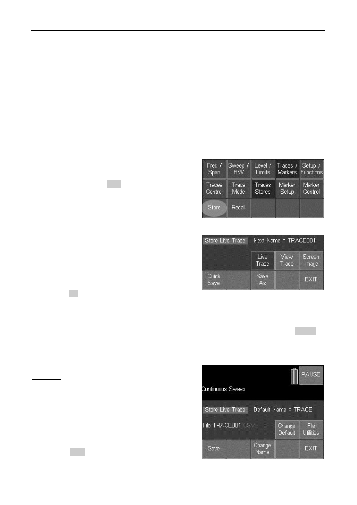
5 File Storage, File Types and USB Connections
Quick
Save
Save
As
The instrument incorporates a large Flash based disk drive for the storage of a variety of
different file types including Traces, Screen Images and Instrument Set-ups. When the
upgrade pack (U01) is fitted it may also include Logging Files, Limit Pattern Tables and
Amplitude Compensation Tables.
The instrument filing system provides a consistent method for storing, recalling, renaming,
deleting and copying files. Files can be transferred to and from a personal computer for
backup, analysis, printing and documentation purposes.
Whenever files are being accessed, the front panel LED marked Disk flashes. Depending upon
the file operation in progress, there may be a significant delay before further key operations are
possible.
5.1 Storing Traces or Screens
Storing of Traces or Screen Images is controlled from
the menu function:
Traces/Markers > Traces/Stores > Store.
(as described in section 4.6.4)
This function enables a trace or screen image to be
stored as a file within the internal memory. (N.B.
external memory cannot be used to store files
directly, although files can be copied to external
memory later).
The menu keys are replaced by a control screen as
shown.
The top row of keys sets what will be stored: the Live
Trace, the View Trace, or a Screen Image. The
currently selected file type is shown in the green box
above the keys.
See section 5.7 for an explanation of Trace files and
Screen Image files.
There are two methods for saving to a file: Quick Save and Save As.
stores the trace or screen under an automatically incrementing name (e.g.
TRACE001 etc.) as set by the Default name as described below in section 5.1.1.1.
The key can be pressed repeatedly to store traces/images as they appear. The next
name that will be used is shown in yellow within the area above the keys.
halts the trace update (causing the sweep
status key to go to Pause) and enters the
next screen as shown.
The auto-allocated file name is shown (based upon
the current default file name), and pressing Save will
store the file under that name. However, the option
also exist to change the name before saving.
Pressing Change Name brings up an alpha-numeric
keypad which can be used to enter any name of up to
eight characters that the user may choose.
See section 5.6.1.
Page 30
Page 32
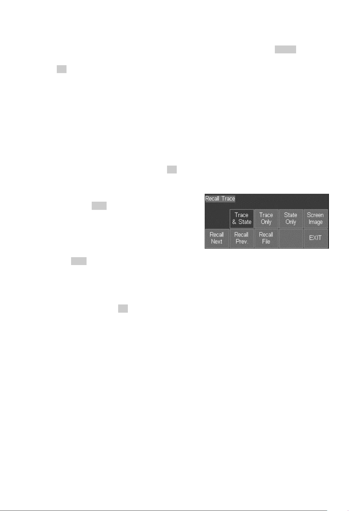
Pressing Save completes the storing of the file under the chosen name.
The default name can also be changed by pressing
Change Default. Any name of up to five characters can be used - see section 5.1.1.1 below.
It is also possible to delete or rename files from this screen by pressing File Utilities - see
section 5.5.
5.1.1.1 Default File Name Rules
Default names are always five characters long, but the user can choose to enter less than
five characters and the system will add the appropriate number of underscores at the end.
The five characters are followed by a three digit number that starts at 001 and autoincrements up to 999.
Deleting files will have no effect on the increment system so that, if the user had created
fifteen files and then deleted them all, the next file saved would still have the number 016.
Should the number reach 999, the auto increment will start again at 001. If this file already
exists, the user will be prompted to delete or rename files or to change the default name.
If the user needs to check the list of existing stored files, or to rename or delete files, this can be
done by pressing File Utilities - see section 5.5.
5.2 Recalling Traces and Images
The Recall function from the Traces/Stores sub-group
menu (see section 4.6.4) creates a control screen as
shown.
The top line of keys enable the selection of the type
of file to be recalled.
Trace files can be recalled in three different ways,
Trace & State, Trace Only, or State Only
See section 5.7.1 for an explanation.
Screen images can also be recalled from this screen. A recalled screen image overwrites the
existing graticule and annotation area. Recalling an image takes around three seconds, with
the image building from the bottom upwards.
Pressing Recall File opens a file list which can show any of the currently stored files of the
selected type. See section 5.4 for an explanation of the File Recall screen.
Pressing Recall Next or Recall Prev. recalls the next or previous file in the list without the need
to re-enter the File Recall screen. This is particularly useful when searching through stored
screen images.
5.2.1 Traces and States
A trace file represents the swept trace as appears upon the screen along with information that
defines the frequency span, RBW, VBW and reference level at the time that it was stored. The
latter information is referred to as the State.
When a trace file is recalled, the user can choose to recall the whole file (Recall Trace & State),
the trace amplitude values only (Recall Trace) or the State values only (Recall State).
Whenever the State is recalled, the spectrum analyser set-up is changed to match the
parameters within the recalled file.
Page 31
Page 33
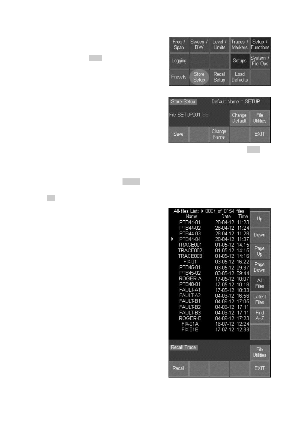
5.3 Storing Instrument Set-up Files
Storing of Instrument Set-ups is controlled from the
menu function:
Setup/Functions > Setups > Store Setup.
(as described in section 4.9.1)
This function enables a complete instrument set-up to
be stored as a file within the internal memory. (N.B.
external memory cannot be used to store files
directly, although files can be copied to external
memory later).
The menu keys are replaced by a control screen as
shown.
The auto-allocated file name is shown (based upon
the current default file name), and pressing Save will
store the file under that name. However, the option
also exist to change the name before saving.
Pressing Change Name brings up an alpha-numeric keypad (see illustration in section 5.6.1)
which can be used to enter any name of up to eight characters that the user may choose.
In the event that a file with that name already exists, a warning message will be displayed.
The default name can also be changed by pressing Change Default. Any name of up to five
characters can be used - see section 5.1.1.1
It is also possible to delete or rename files from this screen by pressing File Utilities - see
section 5.5.
5.4 File Recall Screen
The recall screen for any file type uses the whole of
the display area in order to include a file list. The list
consists of the file name (without its extension) the
date of storage (in format dd/mm/yy) and the time of
storage (in 24 hour format hh:mm). A moveable
pointer operated by the Up and Down keys shows
which file is to be executed.
The keys that control the file selection are in a vertical
list on the right hand side.
One screen can show 20 files simultaneously.
Pressing Page Up or Page Down scrolls through the
files in blocks of twenty.
By default, files appear within the list in date/time
order with the oldest files at the top.
Pressing All Files returns to this listing type at any
time.
Pressing Latest Files will show a screen of up to 20
files that represent the most recently stored or
recalled files.
Files can also be found from their starting character
using File A-Z.
Page 32
Page 34
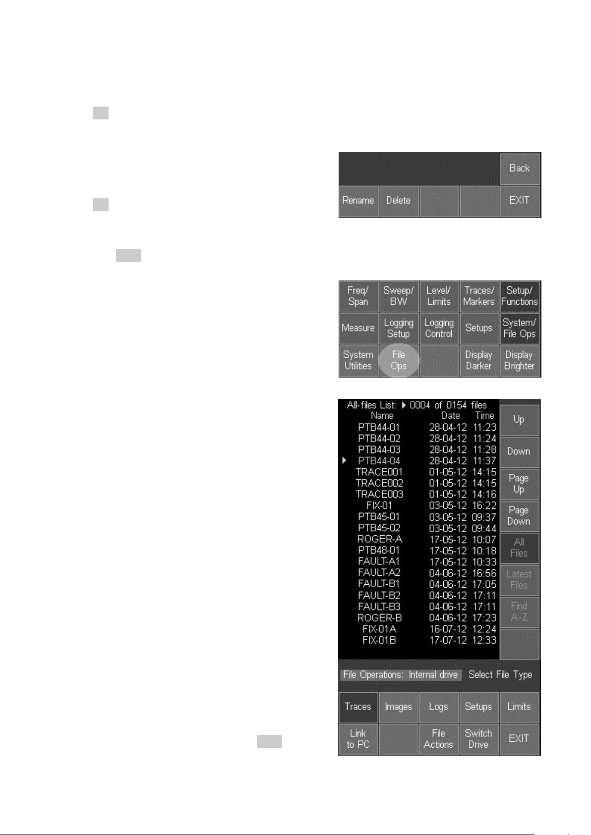
Pressing Find A-Z brings up an alpha numeric keyboard. When a character is pressed the
keypad disappears and the listing then shows only files that start with that character.
Pressing Recall executes the file operation.
It is also possible to delete or rename files from this screen by pressing File Utilities - see
section 5.5.
5.5 File Utilities Screen
Store and Recall screens include a File Utilities key
which enables files to be renamed or deleted.
The layout is similar to a File Recall screen - see
section 5.4 .
Pressing Rename brings up the alpha-numeric keypad
from which the file name can be changed.
See section 5.6.1 for an explanation of file renaming.
Pressing Delete asks for confirmation before
permanently deleting the selected file.
5.6 File Operations Screen
The File Operations screen is an extended version of
the File Utilities screen provided for Store and Recall.
It can be used for all types of file, supports external
Flash memory drives, and also provides access for the
“Link to PC” USB connection.
File Operations is selected from the Setup/Functions
menu:
Setup/Functions > System/FileOps > File Ops.
The upper row of keys enables the file type to be
selected (Traces, Images, Setups etc.).
The upper section of the screen shows a file list for the
selected file type, and is similar to the File Utilities
screen except that the options of Latest Files and Find
A-Z are not available.
The lower row of keys provides further options and
actions.
Pressing Switch Drive enables the files present on an
external USB Flash drive to be listed in place of the
internal drive. If no external drive is connected, the
key will have no effect.
Pressing the key repeatedly alternates between the
two drives. The currently selected drive is displayed
within the green box.
On the first occasion that the external drive is
accessed there will be a delay and a warning
message will be displayed - see section 5.6.4.
Page 33
Page 35
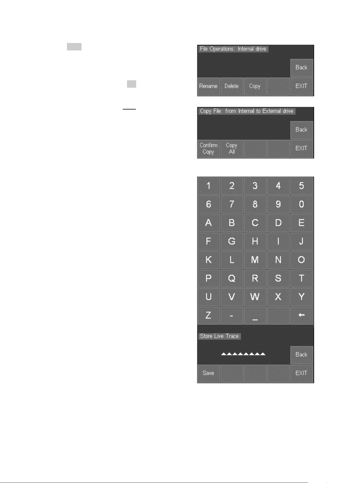
Pressing Link to PC causes all spectrum analyzer operation to be suspended and enables a
connection to be made to a personal computer.
See section 5.6.5 for a detailed explanation.
Pressing File Actions changes the screen to provide
options of Rename, Delete or Copy.
Rename and Delete operate in a similar way as for the
File Utilities screen - see section 5.5.
The Copy function copies a file from the currently
selected drive. Files can therefore be copied from the
internal drive to the external drive or vice versa by
using Switch Drive on the previous screen.
It is also possible to copy all files of the selected file
type by using Copy All.
5.6.1 Editing File Names
Editing a file name (Store File screen) or renaming a
file (File Utilities or File Ops screens) uses an alpha
numeric key matrix. The matrix replaces the upper
screen area.
The whole of the required name must be entered. It is
not possible to edit an existing name character by
character.
The new name appears at the bottom of the screen
replacing the eight triangles shown in the illustration.
Names can be from one to eight characters long and
can include upper case letters, numbers, dash (-), and
underscore ( _ ).
Corrections can be made during entry using the backspace key.
In the event that a file with that name already exists, a
warning message will be displayed.
Pressing Save applies the new name and returns to
the previous screen.
Pressing Back returns to the previous screen without
applying the new name.
Pressing Exit leaves the selected filing system function
immediately.
Page 34
Page 36

5.6.1.1 File Names Created or Renamed Externally
Files may be created externally or created within the instrument and renamed externally (e.g.
using Link to PC mode). Such files may have long file names and/or include lower case
characters and additional characters such as ?.
The instrument will correctly list all such files that conform with an 8.3 naming system and which
have the correct extension for the relevant folder. Where the file name exceeds eight
characters, it will truncate the file name using a ~1 convention.
Files with the wrong extension, or which have been placed in the wrong folder will not be visible
to the instrument filing system. See section 5.7 for a description of file types and their file
extensions.
5.6.2 Internal Filing System Organisation
The organisation of the instrument filing system is not visible to the user from within the
instrument. Although a folder system exists, files are automatically placed into, or retrieved
from, the correct folder whenever a particular type of file is being used.
Similarly, when an external flash drive is connected, the instrument will automatically select the
correct external folder for the current file type.
The folder structure of the internal drive is only visible when linked to a PC - see section 5.6.5.
5.6.3 Understanding USB Connections
The instrument has two USB ports only one of which may be used at a time. The required port
is accessed by a sliding shutter which ensures that only the exposed port can be used.
The Type A port presents a USB host interface which will accept flash drives conforming to the
USB Mass Storage Class (MSC). Drives with capacities from 32MB to 32GB are supported.
This port is not compatible with any other class of device including the HUB class. If an
unsupported device type is connected a message will be displayed to alert the user.
NOTE: Certain small capacity USB flash drives have been seen that try to connect as a hub
before exposing the MSC device. This type of flash drive is not compatible and cannot be used
with this instrument.
When a compatible flash drive is connected to the instrument there will be no activity until the
Setup/Functions > System/File Ops > File Ops control screen is called up, then the Disk light
will flash and the Switch Drive key will become active. This key will allow access to the files
stored on the flash drive. The Copy key in the File Actions control screen will also become
available. See section 5.6.4 “Using an External Flash Drive” for more information on reading
and writing the flash drive.
The Mini B port is for connection to a PC and has two possible uses, each will cause the
instrument to expose a different device type to the PC. When the instrument is powered on the
Mini B port is inoperative and the PC, if connected, will not be able to 'see' the instrument. The
correct device type will be exposed when the user performs an appropriate action. The two
types of device that the instrument can expose are Mass Storage Class (MSC) and
Communications Device Class (CDC). These classes and their uses are discussed in the
following paragraphs.
The PSA will expose the MSC when the user executes Setup/Functions > System/File Ops >
File Ops and then chooses the Link to PC option from the File Ops control screen. See section
5.6.5 “Linking to a PC via USB” for more information.
The instrument will expose the CDC when the user executes Setup/Functions > System/File
Ops > System Utilities followed by Status/System > Screen > View on PC. This function is only
available with Option U01 enabled. For more information see 13 Appendix A “View on PC”.
Page 35
Page 37

It should be noted that CDC is used only for screen data exchange when View on PC is
selected. It is not possible to transfer file data while in this mode. To exchange files between
instrument and PC requires MSC and in this mode View on PC is not available.
The user can, however, switch freely between these modes by executing the key sequences
above but connection to the View on PC application will be lost when Link to PC is selected.
5.6.4 Using an External Flash Drive
The USB Type A connector on the left hand side of the instrument is arranged as USB Host
and is intended exclusively for the connection of a USB Flash Drive.
This enables files to be copied to and from the internal memory of the instrument. Note that
files cannot be loaded from or saved to external memory directly.
Copy operations are performed using the File Ops (File Operations) function - see section 5.6.
The instrument pre-defines a folder system for the USB Flash Drive whereby different file types
are placed in specific folders. These folders are automatically created when the File Ops
function is selected with a Flash Drive plugged in.
A master folder is created called PSA within which are sub-folders named TRACES, IMAGES,
SETUPS, LOGS, and TABLES. Files copied from the instrument onto the external drive are
automatically placed into the correct folder. However, where files are being placed onto the
external drive from a personal computer, they must be put into the correct folder or it will not be
possible to copy them onto the instrument.
Note that, whenever the File Ops function is first used after a USB Flash Drive has been
plugged in or the instrument has been switched off, the files on the Flash Drive will be
interrogated and an information message will appear asking the user to wait for this to take
place.
If the Flash Drive is of large capacity and/or contains a large number of files, the interrogation
could take a long time. If the user wishes to abort this procedure, they may do so by simply
unplugging the Flash Drive. To avoid long delays, it is recommended that Flash Drives
containing large numbers of un-related files are not used.
Note that it is not possible to connect a USB Flash Drive if the USB Link to PC connection is in
place.
5.6.5 Linking to a PC via USB
The USB Type Mini B connector on the left hand side of the instrument is arranged as USB
“device” and is intended exclusively for connection to the USB port of a personal computer for
the transfer of files to or from the internal memory of the instrument.
The connection should be made using the cable supplied, which is a standard USB Mini B plug
to USB Standard A plug. Note that it is not possible to use the USB Link to PC when a USB
Flash Drive is connected.
“Link to PC” mode is selected via Setup/Functions > System/FileOps > File Ops > Link to PC
see section 5.6. When the key is pressed all spectrum analyzer activity is suspended and the
instrument waits for the PC to recognise its Flash based disc drive and “log it on”.
When the link is enabled, the internal drive of the instrument appears on the PC as a removable
disc drive. When in this condition, the PC is in control of the link and file operations are
performed on the PC using Windows Explorer or a similar file system manager.
When in this mode, all of the user area of the internal drive becomes accessible. It is
therefore possible to rename files and directories, delete directories or to add invalid
files. Care must be taken NOT to do this.
The internal drive contains a master folder named PSA within which are five folders: TRACES,
IMAGES, SETUPS, LOGS, and TABLES. Only the correct file types must be placed into these
folders, no files should be placed in the Root folder and no additional folders created.
Page 36
Page 38

Note that it is possible to place files with long filenames into the folders provided that the
extension is correct and the files themselves are valid - see section 5.6.1.1.
The link can be closed by pressing the EXIT hard key. When this happens, the instrument rechecks its filing system in order to ensure that changes have not been made that would cause
system problems. This may take several seconds.
When this has been completed, normal spectrum analyzer operation resumes.
5.7 File Types
The basic instrument uses three file types: Traces, Images and Setups. If option U01 is
installed, several further file types become available.
5.7.1 Trace Files
A trace file represents the swept trace as appears upon the screen. A trace file can be recalled
to the screen as a reference trace (purple).
The file consists of a set of 271 values representing the trace amplitude from left to right across
the screen in CSV (comma separated variable) format, plus additional information that defines
the frequency span, RBW, VBW and reference level.
The latter information is referred to as the State. When a trace file is recalled, the user can
choose to recall the whole file (Recall Trace & State), the trace amplitude values only (Recall
Trace) or the State values only (Recall State). Whenever the State is recalled, the spectrum
analyser set-up is changed to match the parameters within the recalled file.
Trace files are small being a few kilobytes each. Within the instrument they use an 8.3 naming
format with the extension .CSV. A maximum of 999 files can be stored within the internal
memory of the instrument. Trace files can be copied to a PC and imported into graphing
programs such as Excel, MathCad etc.
Trace files can also be displayed using PSA-Manager software which is supplied with
Option U01.
5.7.2 Screen Image Files
A screen image file represents a "snapshot" of the whole of the screen excluding the key area.
A screen file can be recalled in a similar way to an image on a digital camera, whilst sweeping
of the spectrum analyser is suspended (Paused). It can also be exported to a PC and printed
for documentation purposes.
Screen files are indexed colour bitmaps of about 50 kilobytes in size. Within the instrument
they use an 8.3 naming format with the extension .BMP A maximum of 999 files can be stored
within the internal memory of the instrument. Screen files can be copied to a PC and imported
into photo viewing and editing programs such as Windows Picture and Fax Viewer, Paint,
Photoshop etc.
Image files can also be displayed using PSA-Manager software which is supplied with
Option U01.
5.7.3 Setup Files
A setup file records the complete state of the instrument at the point that it was saved, including
marker positions, the view trace and the reference trace.
Setup files are small being a few kilobytes each. Within the instrument they use an 8.3 naming
format with the extension .SET. A maximum of 999 files can be stored within the internal
memory of the instrument. Setup files can be copied to a memory stick or onto a PC for backup
purposes, but have no function outside of the instrument.
Page 37
Page 39

5.7.4 Other File Types
When Option U01 is fitted (see section 6) three other file types can exist. These are
Compensation Table files, Limit Pattern files, and Logging files. Details of the functions are
provided within section 6 of the manual.
5.7.4.1 Compensation Tables
Compensation tables are normalised files of amplitude versus frequency which must be created
outside of the instrument using PSA-Manager software. They are a few kilobytes in size.
They files have the extension .CMP and are located in the folder named TABLES. Files can be
transferred using either a USB Flash drive, or by direct connection to the USB port of a PC.
5.7.4.2 Limit Pattern Tables
Limit pattern tables are normalised files of amplitude versus frequency which must be created
outside of the instrument using PSA-Manager software. They are a few kilobytes in size.
They have the extension .CSV and are located in the folder named TABLES. Files can be
transferred using either a USB Flash drive, or by direct connection to the USB port of a PC.
5.7.4.3 Logging Files
Logging Files record multiple entries of sweep data in response to a variety of trigger signals.
They can contain several types of data and are variable in size up to tens of megabytes. They
have the extension .LOG and are located in the folder named LOGS.
The files are created within the instrument and must be transferred to a PC for analysis using
PSA-Manager software. Files can be transferred using either a USB Flash drive, or by direct
connection to the USB port of a PC.
6 Upgrade Option U01
The capabilities of the instrument can be enhanced by installing the upgrade option U01 which
adds additional firmware to the instrument.
Option U01 can be downloaded from the Aim-TTi website and can be installed by the user
without any requirement to return the instrument to its supplier. Activation of the upgrade is
achieved via an activation code which can be purchased from Aim-TTi, or from our distributors
and agents across the world.
6.1 Additional Functions from Option U01
The following facilities will be incorporated. Additional facilities may also have been added see the Aim-TTi website for up to date information.
6.1.1 Logging of Values, Traces or Screens
The Logging function enables results to be saved into log files in response to a timer or to a
trigger event. Individual amplitude values, complete traces, or full screen images can be saved.
See section 4.8.1 for more information.
6.1.2 Triggering
The triggering function enables sweeps or logging to be triggered in response to an internal or
external trigger event. The internal trigger event can be generated by the Limits function.
See section 7.4 for more information.
Page 38
Page 40

6.1.3 Limit Lines and Patterns
Limit lines and patterns can be shown on the display, and compared with the trace. They can
be used to trigger a logging event, generate an audible warnings or output a trigger pulse.
Limit lines are simple straight lines whereas limit patterns are frequency dependent amplitude
limits that are stored as files. Two limits can be used simultaneously.
See section 7.6 for more information.
6.1.4 Level Offsets
The level offset function enables the level values for the graticule and markers to be corrected
for external attenuation or gain. Compensation can also be made for signals coming from a
75 source.
6.1.5 Compensation Tables
Compensation tables are lists of amplitude versus frequency which enable frequency related
amplitude variations from antennae or transducers to be compensated for within the spectrum
analyzer. Compensation tables are stored as files. See section 7.5.2 for more information.
6.1.6 View on PC
View on PC places the instrument into a special mode in which the graphics of the display are
sent to a PC via USB. The screen can then be viewed at any size using PSA-View PC
software. See section 13 (Appendix A) for more information.
6.1.7 Custom Presets
Custom Presets enables multiple presets (set-ups) to be saved/recalled just by entering a
number. See section 7.2.5.
6.1.8 PSA-Manager Software
PSA-Manager is a Windows based software application which is used in conjunction with the
instrument. It provides the capability for displaying and printing Traces and Screen Images,
display and analysis of Log files, and creation of Limit Patterns and Compensation Tables.
See section 13 (Appendix A) for more information.
Page 39
Page 41
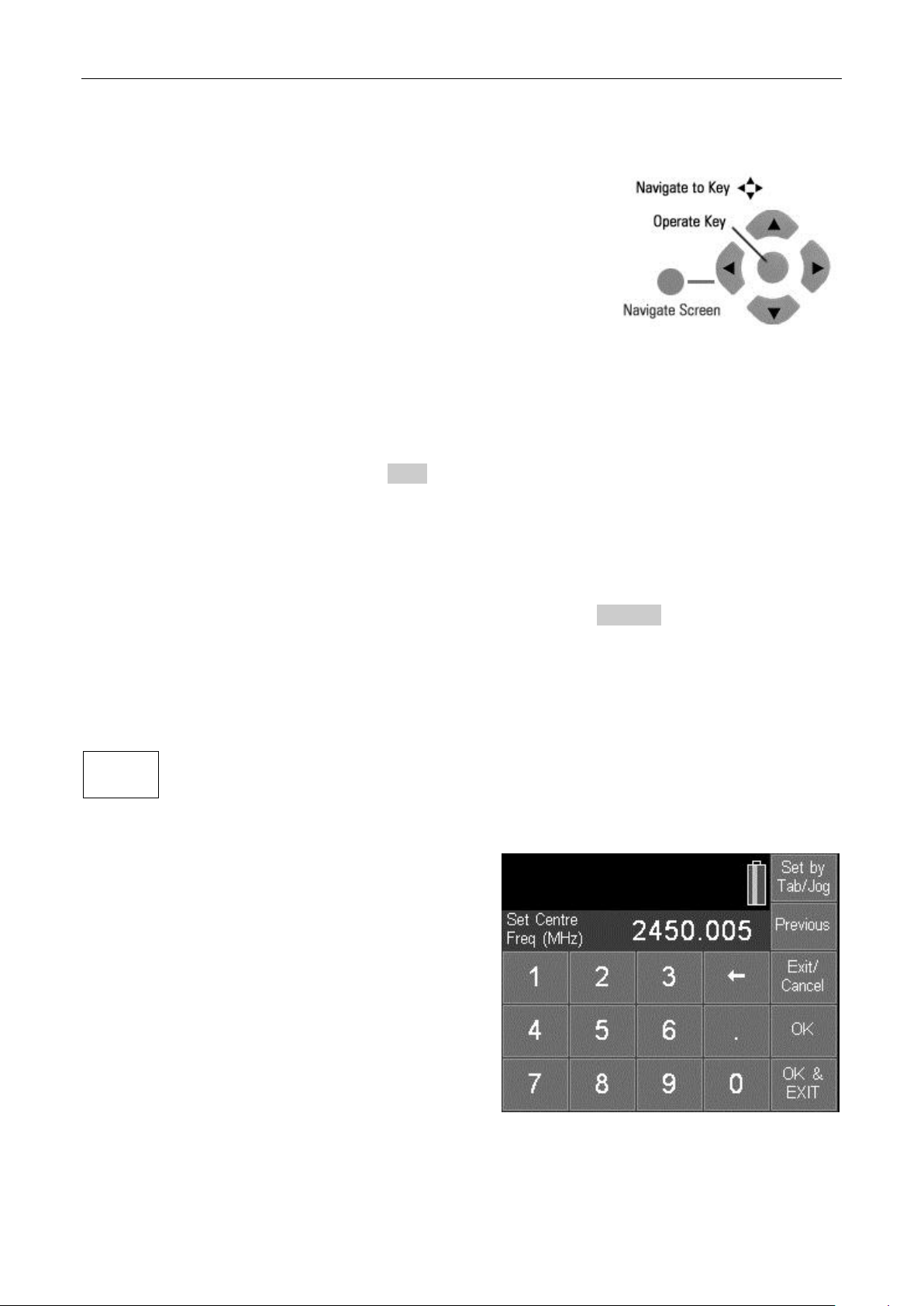
7 Further Notes on Operation
Set
Centre
7.1 Operation using the Hard Keys Only
Although the instrument is designed to be operated via the touch
screen, it is also possible to operate it using only the hard keys.
This may be appropriate in particular circumstances such as
when the user is wearing gloves.
Hard-key-only operation is activated by pressing the circular
button marked Navigate Screen which then illuminates. This
changes the function of the five Navigator keys from controlling
the Markers to controlling the position of the on-screen key
highlight.
The highlight position is shown by a change in the key color to purple. Pressing the centre
button operates the key.
Almost all menu functions can be operated in this way. Pop-up menus and other special
function screens can be exited by pressing the EXIT hard key. An exception is the Set by
Tab/Jog function, described in section 7.2.2 , where the horizontal and vertical navigator keys
operate the tab and jog functions respectively.
Note that, if a touch-screen key is pressed directly, the "hard-key only" mode is cancelled and
the Navigate Screen button ceases to be illuminated. To re-enable the mode, the button must
be pressed again.
Whenever the navigator mode is changed, an information box appears similar to that shown
above. If preferred, this reminder can be turned off - see section 4.10.3.3.
7.2 Setting Frequencies
The control screens used for setting frequencies are common to Set Centre, Set Span, Set
Start, Set Stop, Set Step and Marker Manual Set. The following illustrated example is for Set
Centre but is similar for all other frequency setting functions.
pressing this key will bring up either the Set by Keybd (set by keyboard) screen or
the Set by Tab/Jog screen depending upon which one was last used for setting that
frequency parameter.
7.2.1 Set by Keyboard
This control screen replaces the menu with a 0 to 9
keyboard. The frequency is entered in MHz using
the decimal point if required (maximum resolution
0.001MHz). Frequencies can be entered in whole
MHz when kHz resolution is not needed.
Entry errors can be corrected with the back-space
key ().
Pressing OK sets the entered frequency without
leaving the control screen. The frequency value is
cleared ready for entering a new value.
Pressing OK & Exit sets the entered frequency and
returns to the menu.
Pressing Exit/Cancel returns to the menu without setting the entered frequency.
Pressing Previous returns the frequency to the value directly prior to the last frequency entry.
Pressing Tab/Jog changes to the alternate control screen as detailed below.
Page 40
Page 42
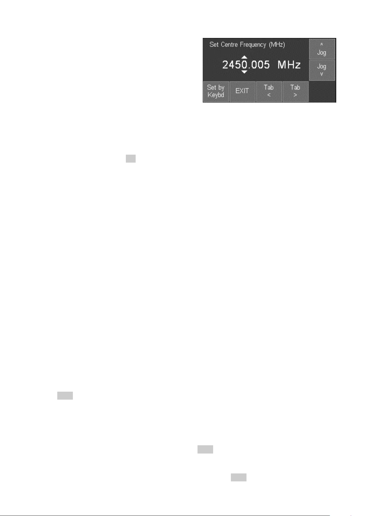
7.2.2 Set by Tab/Jog
This control screen replaces the menu with a display
of the existing frequency and enables it to be
changed.
Pressing either of the Tab keys moves the arrows
left or right along the digits.
Pressing either of the Jog keys increments or
decrements the value of that digit.
The Jog keys auto-repeat, and the new frequency is accepted and executed after a delay of
around two seconds.
Pressing Exit returns to the menu. Pressing Set by Keybd changes to the alternate control
screen as detailed above.
Note that when Navigate Screen mode is selected, the navigator keys perform the tab/jog
function directly - see section 7.1.
7.2.3 Shortcuts to setting a Specific Frequency Span
Narrower Span
Having set a frequency span in which the signals of interest are visible, the user may wish to
examine a specific part of the span at greater resolution.
If the point of interest is the highest level within the current sweep, it can be moved to the centre
of the screen from the Centre sub-group menu (Freq/Span > Centre > Set C=Pk).
Alternatively, marker M1 can be placed at the point of interest and moved to the centre of the
screen from the Centre sub-group menu (Freq/Span > Centre > Set C=M1).
Once the point of interest is in the centre of the screen, the resolution can be increased using
the Zoom In function from the Span sub-group menu (Freq/Span > Span > Zoom In/Out).
An alternative method which enables a more precise span to be set is to place marker M1 at
the start of the area of interest and marker M2 at its end. The new span is then set from the
Start/Stop sub-group menu (Freq/Span > Start/Stop > Start=M1,Stop=M2).
Wider Span
Having set a frequency span in which the signals of interest are visible, the user may wish to
examine a wider span in order to see further signals not currently visible.
One method of doing this is to zoom out from the Span sub-group menu (Freq/Span > Span >
Zoom) which shows frequencies both above and below the current span.
Alternatively, the user may wish to look only at frequencies above (or below) the current span.
This can be done from the Start/Stop sub-group menu (Freq/Span > Start/Stop > Fix Start or
Stop). Once the start or stop frequency is fixed, the word Fix is displayed next to its frequency
at the top of the screen. The Step Up and Step down keys can then be used to increase or
decrease the opposite frequency only. Pressing the key again will cancel the condition. See
section 4.1.3.
7.2.4 Repetitive Operations
A common requirement for a spectrum analyzer user is to change repetitively between two or
more frequency ranges. The PSAxx02 provides several methods for doing this.
1. When setting the centre frequency using the keyboard, the Previous key can be used to
toggle between two centre frequencies - see section 7.2.1. The same facility is provided for Set
Span, Set Start and Set Stop.
2. Frequency Presets, selected via the Frequency/Span menu group, enable up to six
frequency spans to be stored and rapidly recalled - see section 4.1.5. Only Centre/Span or the
Page 41
Page 43
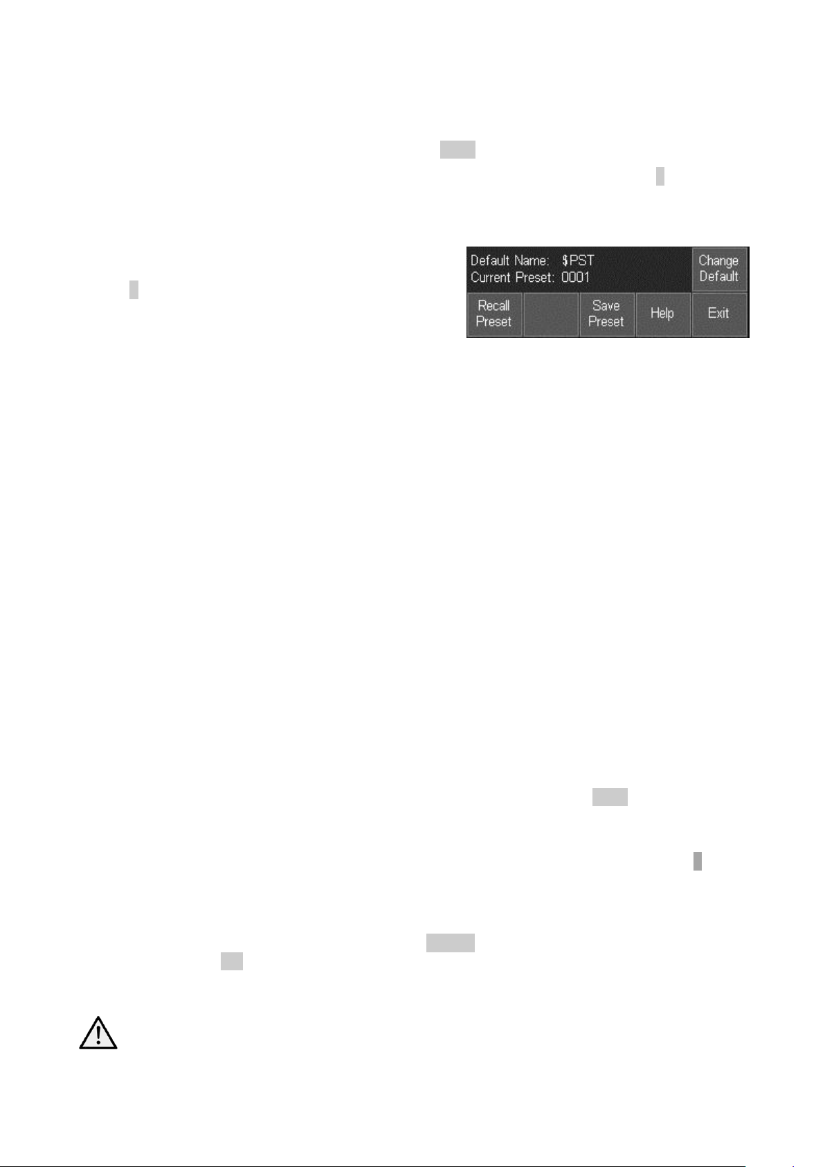
equivalent Start/Stop frequencies are stored. Other parameters such as RBW are not affected
(unless set to Auto).
3. Trace States are files which contain not only the frequency span, but the RBW, the Level
setting and the graticule scale and units. Up to 999 trace files can be stored and are recalled
from the Traces/Stores control screen - see section 4.6.1.
4. The hard key marked “Presets” brings up a menu of set-up states - see section 0. Note,
however, that these change many parameters of the instrument simultaneously.
7.2.5 Using Custom Presets (when available)
Custom Presets is only available when Option U01 is
fitted. It is accessed using the Presets hard key - see
section 0.
Pressing the Custom Presets key brings up a menu
as shown.
Custom Presets is an extended version of the User Preset from which multiple presets can be
saved or recalled by entering just a number. To save a new preset, set up the instrument as
required and press the Save Preset key followed by a number.
Each Preset is a special type of Setup file stored in the SETUPS directory with a file name of
the form $PST0001 where the $ is fixed and the next three characters (default PST) can be
changed to create multiple groups of presets. The last four characters represent the number by
which the preset is saved or recalled. Any number in the range 1 to 9999 can be used, although
the number of presets simultaneously available is set by the directory limit of 999 files.
Applications for which Custom Presets might be used include frequency selection via channel
numbers, or repetitive steps within a test environment.
7.3 Measuring Relative Amplitude
When both measurement markers are turned on, a readout is provided of the difference
between them in terms of both frequency and level.
A common requirement is to measure the signal amplitude at a specific frequency under
different conditions. The PSAxx02 provides a convenient method of doing this.
Having measured the amplitude in the initial condition using marker M1, the value can be fixed
from the Marker Setup sub-group menu (Traces/Markers > Marker Setup > Fix/Unfix M1). The
M1 readout shows Fx at the left hand side. With the new condition applied, the measurement
can be made again by moving M2 to the same frequency using the key Move M2 to M1. The
difference in amplitude level can then be read directly.
To return M1 to normal operation, press Fix/Unfix M1 again. See section 4.7.1.
7.4 Triggered Operation
Triggered operation is only available when the upgrade option U01 is fitted (see section 6).
Triggering is used either to start or stop the sweep, or to initiate logging of sweeps or screen
images. The trigger can be generated manually (by a key press), externally (from the trigger
input) or internally from the sweep in combination with a limit line or limit pattern.
For a description of Triggered Sweep see section 4.4.3.3. For a description of Triggered
Logging see section 7.7.
7.4.1 External Trigger Input
The external trigger input is provided via the 3.5mm jack socket at the top of the
instrument. This can be converted to a standard BNC socket using the adaptor
provided. The selection between positive or negative transition triggering is made from
the Sweep Trigger or Logging Trigger functions. It has a TTL threshold and a high input
Page 42
Page 44

impedance. Maximum input voltage is limited to +/-20V. Voltages above this level could
damage the instrument.
7.4.2 Trigger Output
A trigger output pulse can be generated using the same socket as trigger input (see above).
The signal is generated by the Limits comparator function (see section 7.6.3) and is a positive
going TTL level pulse of approximately 10ms duration from a 1k source impedance.
The trigger output is not available if either sweep trigger or log trigger is set to external
triggering.
7.5 Level Offset and Compensation Tables
These functions are only available when the upgrade option U01 is fitted - see section 6. They
enable the amplitude scaling to be offset to match external attenuation or gain, or to add
frequency dependent amplitude compensation tables to match transducers or antennae. A
description of the menu keys used to control the function is given in section 4.5.4.
7.5.1 Dynamic Range and Maximum Signal
Adding offset or compensation can create confusion as to the maximum and minimum
signal levels that can be viewed.
This could result in the instrument being in amplitude overload even when the displayed
amplitude value is apparently within the instrument range. Where an offset is set to a large
negative value (to compensate for an external gain element) there is a danger that the absolute
maximum signal level could be exceeded resulting in damage to the instrument - see section
3.1.2.
Offset levels and compensation tables should therefore be used with care !
7.5.2 Creating and using Compensation Tables
Compensation tables are normalised files of amplitude versus frequency that are used to
compensate for frequency related non-linearity in antennae or transducers.
The files contain lists of up to 40 frequency/amplitude points. When a file is used by the
instrument, linear interpolation is employed between the points.
Every point on the trace is then changed by the amount calculated from the interpolated
compensation table. Note that this could result in parts of the trace being outside of the
graticule area.
Compensation Tables must be created outside of the instrument using PSA-Manager software see section 6.1.8.
Compensation Table files have the extension .CMP and are located in the folder named
TABLES. Files can be transferred using either a USB Flash drive, or by direct connection to the
USB port of a PC. See section 5 for an explanation of copying and transferring files.
A compensation table file is loaded in a similar way to other types of file using a File Recall
screen - see section 5.4 .
Note that compensation tables and limit patterns are both placed in a folder called Tables and
can therefore appear within the same File Utilities screen. It is possible to toggle between the
two file types by pressing the key marked Tables (toggle).
7.6 Limit Lines & the Limits Comparator | Creating Limit Patterns
These functions are only available when the upgrade option U01 is fitted - see section 6. A
description of the menu keys used to control the function is given in section 4.5.5 .
Two types of limits are available, Lines and Patterns. Up to two limits can be displayed, Limit 1
in red and Limit 2 in blue.
Page 43
Page 45
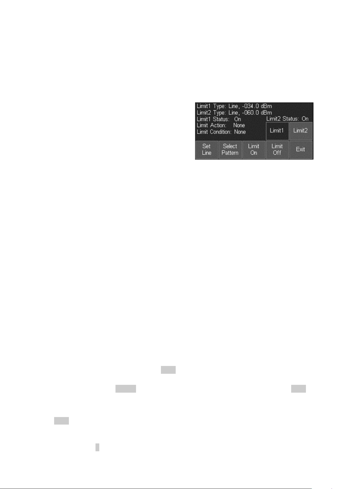
A Line is a simple horizontal line (single amplitude level) that can be set to any value.
A Pattern can have multiple levels and can include vertical steps and angled lines. Patterns are
contained within files that are lists of up to 40 frequency/amplitude points. When a file is used
by the instrument, linear interpolation is employed between the points.
Lines or patterns may be used as simple visual aids to determine whether a signal is within a
specific level range, or they may be used in conjunction with the Limits Comparator to create an
automatic action.
7.6.1 Setting Limits
Pressing the Set Limits key (Level/Limits > Limits >
Set Limits) brings up a control screen as shown.
The keys on the top line select which limit is to be
controlled by the bottom row keys. Where a limit line
or pattern has already been set, it can be turned on or
off using Limit On/Limit Off.
The status of the two limits is displayed within the
area directly above the keys.
Pressing Set Line defines the currently selected limit as a line (if it was previously a pattern)
and brings up a numeric entry keypad or tab/jog system by which the level of the line can be set
numerically in graticule units.
Pressing Select Pattern brings up a list of files from which a limit pattern can be loaded. Limit
pattern files have the default prefix PTN and are placed in the Tables folder. Pressing Recall
from the Recall Limits files screen will load the pattern as the selected limit.
7.6.2 The Limit Comparator
The limits comparator enables automated actions to be selected in response to specified limit
conditions. The actions include audible warning, pulse output from the trigger socket, stopping
of the sweep, or entry into a logging file.
The limit condition is created from the trace being either above or below the limit line/pattern. If
the measurement markers are turned off, or if only M1 is turned on, any part of the swept trace
being above or below the line will create the condition. If both M1 and M2 are turned on, the
limits comparison takes place only on the part of the trace between the markers.
The Limit Condition options are None, Above, Below, Outside or Inside. Where two limits are
being displayed, the limit conditions of Inside or Outside can be used. Note that there is no
concept of an upper or lower limit line. Above means above the higher point of the two limit
lines, Below means below the lower point of the two limit lines, Outside means either above the
higher point or below the lower point of the two limit lines, while Inside means between the
higher and lower points.
The Limit Action can be set to None, Beep, Pulse Out, Beep and Pulse Out together, or
Message. The action only takes places when the sweep has completed. The Pulse Out is
provided at the Trigger socket - see section 7.4.2.
Regardless of the setting of the Trigger Action, it is also possible to use the limit condition to
stop the sweep (see section 4.4.3.3) or to create an entry into a logging file (see section 7.7.5).
7.6.3 Creating and Loading Limit Patterns
Limit Patterns must be created outside of the instrument using PSA-Manager software - see
section 6.1.8.
Limit Patterns files have the extension .CSV and are located in the folder named TABLES.
Files can be transferred using either a USB Flash drive, or by direct connection to the USB port
of a PC. See section 5 for an explanation of copying and transferring files.
Page 44
Page 46
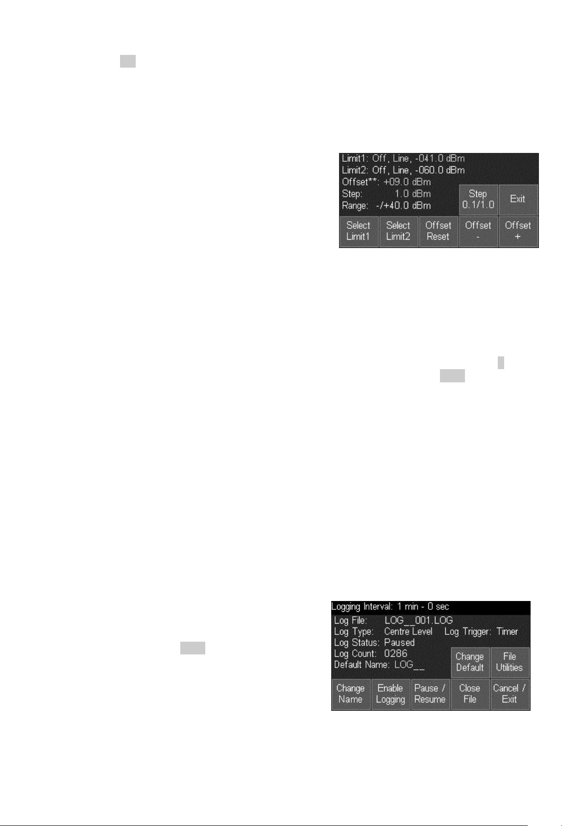
A limit pattern table file is loaded in a similar way to other types of file using a File Recall screen
- see section 5.4. Up to 999 pattern files can be held within the memory of the instrument.
Note that limit patterns and compensation tables are both placed in a folder called Tables and
can therefore appear within the same File Utilities screen. It is possible to toggle between the
two file types by pressing the key marked Tables (toggle).
7.6.4 Limit Offset
The Limit Offset function enables a limit to be offset
from its initial value. It is intended primarily for limit
patterns (which would otherwise have to be
regenerated) but can also be used with limit lines.
The Limit Offset control screen enables a limit to be
“nudged” up or down in steps of 1dB or 0.1dB.
Where a limit has had an offset applied to it, a **
symbol is displayed within the Set Limits control
screen.
7.6.5 Limit Fix/Unfix
This allows a limit pattern, once loaded, to be fixed relative to the screen enabling it to be used
for any centre frequency rather than just the one for which it was created.
7.7 The Logging Function
The Logging function is only available when the upgrade option U01 is fitted (see section 6).
A description of the menu keys used to control the function is given in section 4.8.1.
The logging function saves results into log files within the memory of the instrument. The type
of result saved can be selected as Centre Level (logs only the amplitude at the centre
frequency), Peak Level (logs the frequency and amplitude of the highest peak in every sweep),
Full Trace (logs the whole trace) or Screen Image (logs the whole screen as a bit-map image).
The saving of an entry into the file can be after every sweep (continuous) or in response to a
Timer, a key press (manual trigger), the external trigger input, or the Limits function.
Each entry within the file includes the time of the entry as read from the instrument’s real time
clock. Up to 25,000 entries can be saved within a single file with the exception of Screen Image
logging where the entries are limited to 2,500. The saving of an entry takes a finite length of
time varying from 0.1 seconds (centre amplitude or peak value) up to 1.5 seconds (screen
image). Entries are only saved after the sweep has been completed, and the sweep cannot restart until the entry has been saved.
Note that, when a logging file is “enabled”, the sweep mode is automatically set to Repeat and
the sweep trigger is set to Free Run. No changes can be made to the set-up of the analyser
while logging is in progress.
7.7.1 The Logging Control Menu
Selecting Logging Control from the Logging subgroup menu (see section 4.8.1) opens a new control
screen as shown opposite.
The type of data to be logged, the trigger type, and
the timer interval (if used) must be set prior to
entering Logging Control. This information is shown
within the area above the keys.
Similarly the spectrum analyzer state (frequency span, level etc). must also have been set-up in
advance.
Page 45
Page 47

Once logging has commenced it is not possible to make any changes to the instrument’s set-up
without closing the logging file. It is also not possible to turn the instrument power to Off without
closing the file first.
Change Name: the name of the logging file that will be created is displayed at the top of the
menu area. The file name is an auto-incrementing numeric of the default file name (shown in
green). Pressing Change Name opens an alpha-numeric keypad from which a user-chosen
name of up to 8 characters can be entered.
Change Default: enables the default file name that will be automatically allocated to the next
logging file to be changed. Standard default file name rules apply - see section 5.1.1.1
Enable Logging: commences the opening of a logging file under the currently displayed name.
An information message is displayed and logging is actually enabled after confirming with the
Status hard key.
Pause/Enable: causes new entries into the current logging file to be suspended and re-started.
However it is not possible to exit from the logging control menu without closing the current file.
Close File: closes and saves the current logging file. Once closed the file cannot be re-opened
(although it can be renamed or deleted). The Log File name changes to the next default name
ready for the next logging file to be enabled.
Cancel/Exit: exits the logging control menu provided that a logging file is not currently enabled
or paused, in which case a warning message is displayed telling the user that exiting will
disable logging and close and save the current file.
File Utilities: displays a list of logging files currently within the instrument. Operates similarly to
other file utilities screens – see section 5.5.
7.7.2 Manual Logging
The logging function can be set via the Log Trigger key to save entries in response to a manual
key press. Both the Run/Stop hard key and the sweep control touch-screen key act as the
manual trigger.
The data that is logged will relate to the sweep that was in progress when the key was pressed.
7.7.2.1 The Run/Stop key and Sweep Control key
When logging, the Run/Stop hard key and sweep control touch-screen key have no function
unless the Log Trigger has been set to Manual, in which case both act as a manual trigger key.
In all other trigger modes (timer, external, limits or continuous) the keys are inactive. However,
the touch-screen key does provide visual feedback of the stages of the logging process. When
no trigger event has yet occurred the key is green and marked Awaiting Trigger. When a
trigger has occurred but the sweep has yet to complete it becomes yellow and is marked
Triggered. When the sweep is completed and the log file entry is being made it becomes red
and is marked Writing File.
7.7.3 Logging from the Timer
The logging function can be set via the Log Trigger key to save entries triggered at a fixed time
interval.
The Timer Setup key enables a time between trigger events to be set between 5 seconds and
100 minutes. However, if the timer interval is set to a short period, the actual time between
logging entries may be considerably longer than the trigger interval. This is because, for each
entry, a sweep must be completed and the data must be saved. If the sweep is set to a wide
span and/or narrow RBW, the sweep time could be several tens of seconds.
The timer is asynchronous with respect to the sweep. Consequently the time between logging
entries will be longer than the timer interval by a variable amount which is a function of the
sweep time. The log entry time stamp represents the time at the end of the logged sweep.
Page 46
Page 48

To achieve the fastest possible logging use Continuous trigger - see section 7.7.6.
7.7.4 Logging from External Trigger
The logging function can be set via the Log Trigger key to save entries on either a positive or
negative going edge applied to the Trigger socket - see section 7.4.1.
The data that is logged will relate to the sweep that was in progress when the trigger signal
occurred.
7.7.5 Logging from Amplitude Limits
The logging function can be set via the Log Trigger key to save entries when a signal is
generated by the Amplitude Limits Comparator. The data that is logged will relate to the sweep
that was in progress when the limit condition occurred.
The Limits function must be set to have a potentially valid condition. See section 7.6 for an
explanation of the Limits function.
7.7.6 Logging Every Sweep (Continuous)
The logging function can be set via the Log Trigger key to save entries continuously, i.e. after
every sweep. The actual speed will depend upon the sweep rate and the type of data being
logged. The fastest possible logging rate is about two per second.
7.7.7 File Sizes and Maximum Logging Times
Logging files can vary in size from a few kB to more than 100MB depending upon the number
of entries and the type of data being logged.
Although the filing system allows up to 999 .LOG files to be stored, the practical number may be
limited by the internal memory size (approximately 1.8GB). Where large files are being created,
care must be taken not to overflow the memory. Memory space can be restored by copying
files to a Flash drive or directly to a PC, and then deleting them on the instrument.
The instrument has the potential to log over very long periods. Where it is required to log for a
period close to or exceeding the battery life, the instrument must be operated from external AC
power.
In the event of the memory becoming full or the power being lost, the current logging file will be
automatically closed.
7.7.8 Viewing and Analyzing Logging Files
The instrument has no capability for viewing the contents of a logging file. Instead, the file must
be copied to a Windows based PC where the file can be viewed and analyzed using the PSA
Manager software - see section 6.1.8.
Log files have the extension .LOG and are located in the folder named LOGS. Up to 999
logging files can be stored within the memory of the instrument. Files can be transferred using
either a USB Flash drive, or by direct connection to the USB port of a PC.
See section 5 for an explanation of copying and transferring files.
Page 47
Page 49

8 Default Settings | Power On State |Hard Reset
8.1 Standard Preset
The standard preset is accessed by pressing the hard key marked Preset. The standard preset
returns the instrument to a set of known conditions as follows (values apply to PSA2702):
Parameters in {brackets} are relevant only if option pack U01 is installed.
Centre Frequency: 1350.5MHz Span: 2699.0MHz
Start Frequency: 1.0MHz Stop Frequency: 2700.0MHz
Step Value: 1.0MHz
RBW: Auto Video Filter: On
Sweep: Repeat, {Sweep Trigger: Free Run}
Reference Level: 0dBm (Atten. On) Units: dBm
Scale: 10dB/div
{Offset: None} {Compensation Table: None}
{Limit 1 & 2 Off}
Live Trace: On Trace Mode Normal
View Trace: Off Reference Trace: Off
Markers: M1 on, position = centre, mode = peak find, M2 off
{Logging: Disabled}
Parameters for the PSA1302 are identical apart from Centre Frequency (650.5Mz), Span
(1299MHz) and Stop Frequency (1300MHz).
The User Preset is a customisable version of the Standard Preset – see section 4.11.1.
8.2 Factory Default Set-up
When shipped from the factory, the set-up of the instrument is as per the Standard Preset (see
above) with the following additions:
Brightness: 40% Auto-sleep: Never
Navigator function: Marker Control Frequency Setting: By Keyboard
Audio Demod. Off (volume = 10) Power-On State: Last Used
Graticule: Normal Trace Avg. No. 16
8.2.1 Restoring to Factory Defaults
The instrument can be returned to its factory defaults condition, as described above, from
Setup/Functions > Setups > Load Defaults (see section 4.9.1).
8.3 Power-On State
The set-up of the instrument each time that it is turned on (from off) is normally set to “Last
Used”. This results in no change occurring when the instrument is powered off and then back
on.
Alternatively, the user can choose to load the User Preset which overwrites the major settings
with ones chosen by the user (see section 4.11.1). This choice is made from:
STATUS >System Utils > Power/Clock > Pwr-On State - see section 4.10.3.2.
Page 48
Page 50
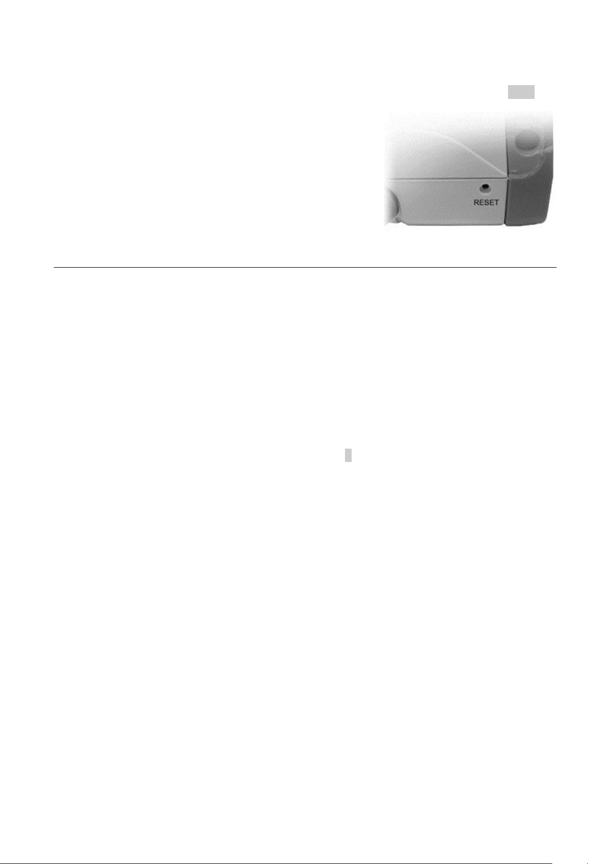
8.4 Unrecoverable Fault Condition - Hard Reset
If the spectrum analyzer gets into a condition in which normal operation is not possible, it can
be returned to normal operation by reloading the Factory Default settings - see section 4.9.1.
However, if it “locks up” (i.e. will not respond to key presses)
or cannot be recovered by using Load Defaults, it can be put
through a Hard Reset.
The reset button is accessed through a small hole at the top
right hand side of the case. It can be operated using the
stylus (or other thin rigid object). Press and hold for longer
than 1 second.
Hard Reset will re-load the operating system, return all
parameters to their factory defaults, and clear all of the nonvolatile buffers. User data and settings that have been saved as files will not be affected.
9 Firmware Updates | Upgrades | Maintenance
9.1 Updating the Firmware
From time to time TTi may make updated versions of the instrument firmware available in order
to add new features or to correct “bugs”. These will be downloadable from the Aim-TTi website
without charge. The current version is displayed within the Status display screens.
The method of updating requires the use of a USB Flash drive. Full information on how to
perform the update will be provided with the firmware file.
9.2 Upgrading the Firmware (Option U01)
Installing option U01 is done in a similar way to a firmware update, but an additional step of
entering an activation code will be needed (see section 6). Full details are provided with the
option.
9.3 Maintenance, Re-calibration & Cleaning
To ensure that the accuracy of the instrument remains within specification, the calibration
should be checked (and if necessary adjusted) annually. Aim-TTi or their agents overseas will
provide a calibration service for any PSA1302/2702 and will repair any PSA developing a fault.
Where owners wish to undertake their own recalibration, this should only be done by skilled
personnel in conjunction with the Service Guide which may be obtained directly from Aim-TTi or
their agents overseas. Recalibration requires the use of a precision signal generator as
specified in the Service Guide
Cleaning: If the unit requires cleaning, use a cloth that is only lightly dampened with water or a
mild detergent. Take particular care in cleaning the touch screen area.
Page 49
Page 51

10 EMC
Spectrum Analyzer – powered by internal battery or Adaptor/Charger
This instrument has been designed to meet the requirements of the EMC Directive 89/336/EEC.
Compliance was demonstrated by meeting the test limits of the following standards:
Emissions
EN61326-1 (2006) EMC product standard for Electrical Equipment for Measurement, Control and
Laboratory Use. Test limits used were:
a) Radiated: Class B
Note: Limits were met without a test object connected; emissions which exceed the levels required
by this standard may occur when the instrument is connected to a test object.
Immunity
EN61326-1 (2006) EMC product standard for Electrical Equipment for Measurement, Control and
Laboratory Use.
Test methods, limits and performance achieved were:
a) EN61000-4-2 (2009) Electrostatic Discharge : 4kV air, 4kV contact, Performance A (A).
b) EN61000-4-3 (2006) Electromagnetic Field, 3V/m, 80% AM at 1kHz, Performance B (A).
Note: The PSA1302 & PSA2702 are sensitive measuring instruments and, if
subjected to a sufficiently large RF field, the interfering signal may show a few dB
above the noise floor even with the SMA input capped (Performance B). In all other
respects the instrument will operate correctly (Performance A) in fields up to 3V/m.
Adaptor/Charger
This AC adaptor/charger has been designed to meet the requirements of the EMC Directive
89/336/EEC. Compliance was demonstrated by meeting the test limits of the following standards:
Emissions
EN55022, radiated and conducted Class B.
Immunity
EN55024:1998 + A2:2003. Test methods, limits and performance achieved were:
a) EN61000-4-2 (2001) Electrostatic Discharge : 4kV air, 4kV contact, Performance A (B).
b) EN61000-4-3 (2002) Electromagnetic Field: 3V/m, 80% AM at 1kHz, Performance A (A).
c) EN61000-4-11 (2004) Voltage Interrupt: ½ cycle 0%: Performance A (B); 1 cycle 0%
Performance B (B); 25 cycles, 70% and 250 cycles, 0%: Performance B (C).
d) EN61000-4-4 (2004) Fast Transient: 1kV peak (AC line), Performance A (B)
e) EN61000-4-5 (2001) Surge: 1kV (line to line), 2kV (line to ground), Performance A (B).
f) EN61000-4-6 (2003) Conducted RF: 3V, 80% AM at 1kHz (AC line & DC Output)
Performance A (A).
Performance Definitions
The definitions of performance criteria are:
Performance criterion A: ‘During test normal performance within the specification limits.’
Performance criterion B: ‘During test, temporary degradation, or loss of function or performance
which is self-recovering’.
Performance criterion C: ‘During test, temporary degradation, or loss of function or performance
which requires operator intervention or system reset occurs.’
Page 50
Page 52

11 Declaration of Conformity
Emissions:
a) EN61326-1 (2006) Radiated, Class B
Immunity:
EN61326-1 (2006) Immunity Table 1, Performance B, referring to:
a) EN61000-4-2 (2009) Electrostatic Discharge
b) EN61000-4-3 (2006) Electromagnetic Field
EC Declaration of Conformity
We Thurlby Thandar Instruments Ltd
Glebe Road
Huntingdon
Cambridgeshire PE29 7DR
England
declare that the
PSA1302 and PSA2702 Portable RF Spectrum Analyzers
meet the intent of the EMC Directive 2004/108/EC and the Low Voltage Directive 2006/95/EC.
Compliance was demonstrated by conformance to the following specifications which have been
listed in the Official Journal of the European Communities.
EMC
Safety – PSA1302/PSA2702
EN61010-1 Pollution Degree 2.
Safety – AC Adaptor/Charger
EN60950-1
CHRIS WILDING
TECHNICAL DIRECTOR
1st October 2012
Page 51
Page 53

12 Specification
Frequency Range:
1 MHz to 2700 MHz in one range - PSA2702
1 MHz to 1300 MHz in one range - PSA1302
Setting Modes:
Centre frequency plus Span, or Start frequency plus Stop frequency
Maximum Span:
2699 MHz (1 MHz to 2700 MHz) - PSA2702
1299 MHz (1 MHz to 1300 MHz) - PSA1302
Minimum Span:
270 kHz, or Zero Span with demodulation
Setting Resolution:
1 kHz at any frequency
Setting Accuracy:
Reference Frequency Accuracy for Start, Stop & Centre (Zero-Span)
frequencies
Initial Accuracy:
Better than ± 10 ppm at 20oC
Stability:
Better than ± 10 ppm over 10oC to 30oC
Ageing:
Better than ± 3 ppm per year
Phase Noise:
Typically -90dBc/Hz at 100kHz offset at 500MHz
RBW:
Selectable as 1 MHz, 280 kHz or 15 kHz
Video Filtering:
Selectable On or Off
Number of Markers:
One, Two, or None
Marker Resolution:
0.1 kHz at all frequencies
Marker Accuracy:
1/270th of Frequency Span ± 0.1kHz + Reference Frequency Accuracy
Frequency Readout:
Display of absolute and difference frequencies for both markers
Display Range:
85 dB
Measurement Units
dBm or dBµV (dB milliwatts or dB micro volts)
Reference Level:
Selectable as -20 dBm or 0dBm (87 dBµV or 107 dBµV)
Ref. Level Accuracy:
Better than ± 1 dB at 50MHz at 10dB below ref. level (20oC ± 5oC)
Level Flatness:
Better than ± 1.5 dB relative to 50MHz over 1MHz to 2700MHz
Amplitude Linearity:
Better than ± 1 dB over 50dB range down from reference level
Noise Floor:
Better than -95 dBm average displayed noise floor for F > 3MHz
(reference level = –20 dBm, RBW = 15 kHz, video filter On)
3rd Order Intermod.:
< –60dBc for two signals(500MHz and 502MHz) at 10dB below
reference level
Harmonic:
< –60dBc at 10dB below reference level (100MHz)
1st & 2nd Image:
<– 55dBc, typically <– 60dBc
Residual Spurii:
<3dB above noise floor
12.1.1 Frequency Measurement
Frequency Span
Reference Frequency Accuracy
Phase Noise
Resolution Bandwidth
Frequency Markers
12.1.2 Amplitude Measurement (Level)
Amplitude Range
Amplitude Accuracy
Noise Floor
Distortion and Spurii
Page 52
Page 54

Amplitude Markers
Number of Markers:
One, Two, or None
Marker Resolution:
0.1 dB
Amplitude Readout:
Display of absolute and difference amplitudes for both markers in
graticule units (dBm or dBuV) or linear units (mV or uW).
Limit Types:
Limit Lines from numeric values, or Limit Patterns from Files. Pattern
files are created using PSA-Manager software.
Number of Limits:
One or two limits on screen. Up to 999 patterns can be stored
Limits Comparator:
Conditions of Above, Below, Inside or Outside creating actions of
beep, stop sweep, log sweep and pulse out
Offset:
Amplitude can be offset by up to +/-50dB to compensate for external
attenuation or gain.
75 Compensation
Compensation can be made for inputs from a 75 source impedance.
Compensation
Tables:
Linearly interpolated tables of up to 40 frequency/amplitude points can
be used. Up to 999 tables can be stored. Table files are created using
PSA-Manager software.
Graticule:
8.5 x 10 divisions light grey graticule. Selectable as normal, dim, or off.
Displayed Points:
271 points per sweep (peak detected).
Live Trace:
Dot-joined trace from current or held sweep. Selectable on or off.
View Trace
Additional trace created from the live trace. Selectable on or off.
Reference Trace:
Trace recalled from a file. Selectable on or off.
Trace Modes:
Normal, Peak Hold, or Average (2 to 48 sweeps)
Sweep Method:
Peak detection for 270 points per sweep. The amplitude of the peak
level found within each sub-span is stored (sub-span = span/270).
Sweep Time:
Set automatically by Span and RBW.
Typically 150ms + 2.3ms/MHz of span for RBW = 1MHz
Typically 150ms + 7ms/MHz of span for RBW = 280kHz
Typically 180ms + 77ms/MHz of span for RBW = 15kHz
Sweep Modes:
Normal (repeat) or Single
Sweep Trigger
(Only with Option U01), External or Limits Comparator
Log Files
Files of up to 25,000 data entries can be created. Up to 999 files can
be stored. Files are read using PSA-Manager Software.
Logged Data:
Log files can be created from Peak Value, Centre Frequency Level,
Complete Sweep, or Screen Image
Log Trigger:
Log entry can be triggered by Key Press, Continuous (every sweep),
External Input, Internal Timer, or Limits Comparator
Timer Interval
Adjustable between 2 seconds and 100 minutes per entry
Time Stamp
Each entry is time stamped from the real-time clock
Amplitude Limits (only with Option U01)
Amplitude Compensation (only with Option U01)
12.1.3 Traces
12.1.4 Sweep
12.1.5 Data Logging (only with Option U01)
Page 53
Page 55

12.1.6 Demodulation (Zero Span mode)
Demod. Modes:
AM or FM
Display:
Carrier amplitude only (horizontal line).
Audio Out:
30 mW into 32 Ohms mono or stereo headphones, adjustable volume,
3.5mm jack socket
Audio Filter
Selectable low-pass filter to attenuate high frequency interference.
2 pole filter with turnover point at approximately 3 kHz.
Display Type:
4.3 inch (10.9 cm) transflective backlit TFT LCD, 480 x 272 pixels total,
16 colours, touch screen.
Graticule:
8.5 x 10 divisions light grey graticule. Selectable as normal, dim, or off.
Memory Type:
Internal non volatile Flash memory (1.8GB nominal).
Store Trace:
Up to 999 traces can be stored under either default file names or user
entered file names. Traces are stored as tables of amplitude versus
frequency and can be imported into other programs, as well as being
recalled to the screen. Traces can be stored from either the live trace
or the view trace and include State information.
Recall Trace:
Recalls any stored trace to the reference trace of the display. The State
can be recalled independently from the Trace
Store Screen:
This function copies the whole screen area (excluding key area) to
memory as a bit-map image. Up to 999 screens can be stored under
either default file names or user entered file names..
Recall Screen:
Recalls any stored screen image to the display.
Store Set-up:
Up to 999 instrument set-ups can be stored under either default file
names or user entered file names. All settings of the instrument are
saved.
Recall Set-up:
Recalls any stored set-up, overwriting the existing settings of the
instrument.
Recall Limits Pattern:
Only with Option U01. Up to 999 limit pattern files produced within
PSA-Manager software can be stored within the instrument.
Recall Compensation
Table:
Only with Option U01. Up to 999 compensation tables produced within
PSA-Manager software can be stored within the instrument.
Store Logging File:
Only with Option U01. Up to 999 logging files can be stored for
download and analysis by PSA-Manager software.
RF Input Connector:
Standard SMA connector (female).
Power Connector:
1.3mm dc power socket for AC power adaptor/charger as supplied by
Aim-TTi.
USB link to PC
interface:
Mini USB connector (5 pin mini B) which acts as a USB “device” for
connection to a personal computer.
USB Flash Drive
interface:
USB standard A connector (USB Host) for connection of USB Flash
memory drive
Audio Connector:
3.5 mm jack socket for demodulated audio out (accepts mono or stereo
plugs).
Trigger connector:
3.5mm mono jack socket for connection of BNC adaptor (supplied).
12.1.7 Display
12.1.8 Memory Storage
12.1.9 Connectors
Page 54
Page 56

Signal Input
Input Connector:
SMA connector, 50 Ohms
VSWR:
1.5:1 typical
Absolute
Maximum
Input Level:
+ 20 dBm or +127 dBµV (2.2V rms) or 50V dc
The PSAxx02 can be operated continuously from mains power using the
AC power adaptor provided by Aim-TTi. This also recharges the
internal battery.
Input Voltage Range:
100V to 240V nominal 50Hz/60Hz. Interchangeable plus for UK, Euro,
USA and Australia are supplied.
The PSAxx02 operates from internal rechargeable batteries. The
batteries are recharged using the AC power adaptor supplied.
Battery Type:
Li-ion 3.7V, 3Ahr nominal
Battery Life:
> 8 hours continuous operation
Recharge Time:
< 3 hours from fully discharged
Auto-Sleep Mode:
To conserve battery life, the system can be set to automatically switch
into sleep mode after a defined time from the last key press. This can
be set between 5 mins and 60 mins (or never).
Size:
192 x 92 x 49mm (7.5 x 3.6 x 1.9”) plus 3mm projection of SMA
connector
Weight:
560 grms (1lb 4oz).
Tilt Stand:
Built-in tilt stand for bench use which angles the unit at approximately
40 degrees to the horizontal.
Screen Protector
For portable use, the tilt stand can be moved from the rear of the
instrument to the front where it acts as a screen protector and sun
shield.
Operating Range:
+5oC to + 40oC, 20% to 80% RH.
Storage Range:
-10oC to +50oC
Environmental:
Indoor use at altitudes to 2000m, Pollution Degree 2.
Electrical Safety:
Complies with EN61010-1.
EMC:
Complies with EN61326.
12.1.10 AC Line Operation
12.1.11 Battery Operation
12.1.12 Mechanical
12.1.13 Environmental and Safety
Page 55
Page 57

13 Appendix A: PSA-Manager and PSA-View Software
PSA-Manager is a Windows* PC application for the creation, editing, analysis and management
of PSAxx02 files. It is compatible with versions of Windows from XP onwards (including 32 and
64 bit versions).
PSA-Manager may be supplied on the CD accompanying the instrument, or may be freely
downloaded from the web site. A secondary application called PSA-View is similarly available.
PSA-Manager Functions
Trace File Display
Trace files downloaded from the instrument can be viewed on the PC.
Limit Patterns Creation
Limit pattern files can be used within the Limits function of the instrument when option U01 is
installed. Limit patterns are tables of amplitude against frequency that are created within PSAManager and uploaded to the instrument.
Limit pattern table files can be created from scratch or imported and edited from CSV files.
Editing tools include both numeric entry and graphical editing.
Compensation Tables Creation
Compensation tables files can be used within the Offset/Tables function of the instrument when
option U01 is installed. Compensation tables are normalised tables of amplitude against
frequency that are created within PSA-Manager and uploaded to the instrument.
Compensation table files can be created from scratch or imported and edited from CSV files.
Editing tools include both numeric entry and graphical editing.
Log File Analysis
Logging files downloaded from the instrument can be viewed and analysed. (The logging
function requires Option U01)
An explanation of how to use PSA-Manager is provided within the program’s own Help function.
PSA-View
PSA-View is an additional PC application which can be used with the View-on-PC function of
the instrument when option U01 is installed. It enables the screen of the instrument to be
duplicated on the PC at any desired size.
The View on PC function places the instrument into a special mode in which the graphics of the
display are sent to a PC via USB. The screen can then be viewed at any size using the
PSA-View application which may be supplied on the CD accompanying the instrument or is
freely available from Aim-TTi website.
To communicate with PSA-View, the USB interface functions as a virtual COM port which can
be controlled by a PC as if it was an RS232 device. The instrument is supplied with a CD
containing a .inf file for the standard Microsoft drivers available in Windows 2000, XP, Vista and
Windows 7; the installation wizard will install the driver (32-bit or 64-bit) appropriate to the PC’s
operating system. Any updates are available via the Aim-TTi website.
Installation of the interface driver is achieved by connecting the instrument to a PC via the USB
cable supplied and selecting Setup/Functions > System/file Ops > System Utilities followed by
Status/System > Screen > View on PC. The Windows’ plug and play functions should
automatically recognise the addition of new hardware attached to the USB interface and, if this
is the first time the connection has been made, prompt for the location of a suitable driver. (If
this does not happen, it will be necessary to open Device Manager on the PC and force a
manual installation of the driver).
Page 56
Page 58

On installing the driver, Windows will establish a virtual COM port within the PC. The number of
the new COM port will depend upon the number of co-existing COM ports. The driver will
remain installed on the PC so that the establishment of a virtual COM port is done automatically
each time the instrument is connected to the PC via USB in the future. The instrument is
assigned a new virtual COM port when it is first connected and the same COM port will be
assigned each time that instrument is subsequently connected.
Once the driver is loaded, and with the instrument still connected to the PC, open the PSA-View
application on the PC. PSA-View will load with two windows open, the graphics window which
will initially contain the message "No Communication Link" and a control window. On the control
window COM Port dropdown select the COM port which is connected to the instrument.
To discover which COM port this is the user can look in Device Manager where the virtual COM
ports are displayed with the name of the device that they are connected to. e.g PSAxx02
Spectrum Analyser (COM8). Once the COM port is selected click on the Connect button and,
after a short delay, the instrument screen data should appear in the graphics window.
Thereafter changes on the instrument screen will also be seen in the graphics window.
Operation of the instrument will slow down a little due to the large volume of data now flowing to
the PC.
To stop viewing on the PC do any of the following:
Close the PSA-View application and disconnect the USB cable
Disconnect the USB cable
Select View on PC again and press Status in response to the information box
Power off the instrument
Set the instrument into Link to PC mode.
Before using PSA-View and the View on PC function, it is advisable to read section 5.6.3 which
explains USB connections in more detail.
* Windows is a trademark of Microsoft, inc.
14 Appendix B: Optional Accessories
At the time of going to print, the following options and accessories were available:
Firmware Upgrade (PSA-U01) – see section 6 .
Fitted Soft Case (PSA2-SC) – protective carrying case with space for accessories
Telescopic Antenna (WB-ANT) – wideband telescopic antenna with SMA connector
Vehicle Charger (PSA-VC) – charger operating from 12V or 24V.
NOTE: All of the above are included within the PSA1302USC and PSA2702USC products.
Page 57
Page 59
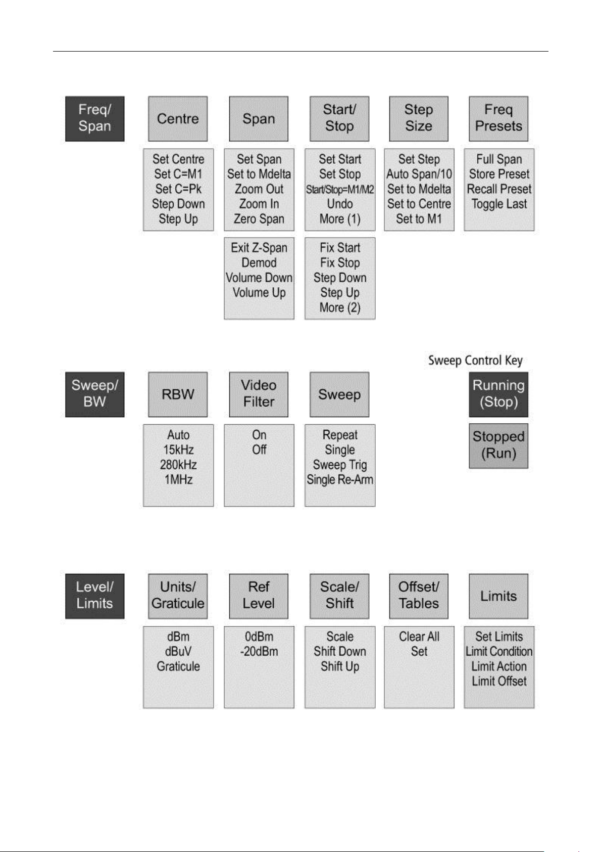
15 Appendix C: Menu Tree Diagram
Page 58
Page 60
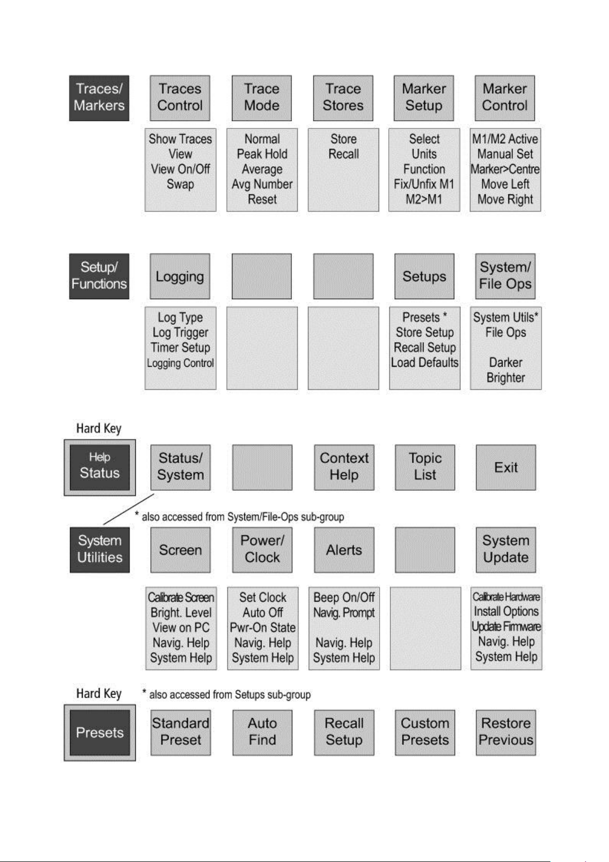
Page 59
Page 61

Book Part No. 48511-1580 Issue 5
 Loading...