THORLABS PAX1000 Operation Manual

Download

Compact Polarimeter

PAX1000 Operation Manual

2019

Version: Date:

1.2 26-Feb-2019

Contents

Foreword 1 General Information 1

2 Getting Started 5

142.6 First Steps

3 Graphical User Interface (GUI) 15

153.1 General

163.2 GUI Overview

173.3 Menu File

11.1 Safety

31.2 Ordering Codes and Accessories

41.3 Requirements

52.1 Parts List

62.2 Operating Principle

72.3 Operating Elements

82.4 Mounting

92.5 Installing Software

203.4 Menu Device

223.5 Menu View

223.6 Menu Tools

223.7 Menu Help

233.8 Status Bar

4 PAX1000 Settings 24 5 Operating Instruction 25

255.1 Alignment Assistance

265.2 PAX1000 Measurements

275.2.1 Measurement Value Table

295.2.2 Polarization Ellipse

295.2.3 Poincaré Sphere

315.2.4 Scope Mode

345.2.5 Long Term Measurement

345.2.5.1 Settings

355.2.5.2 Measurement

365.2.6 Extinction Ratio Measurement

385.2.6.1 ER Measurement Wizard

415.2.6.2 ER Measurement Tool

435.2.7 Virtual Device

435.2.8 Multiple Devices

6 Write Your Own Application 45

466.1 32 Bit Operating Systems

486.2 64 Bit Operating Systems

7 Maintenance and Service 50

507.1 Version Information

517.2 Troubleshooting

8 Tutorial 53

538.1 Polarization of Light

538.1.1 The Nature of Polarization

548.1.2 Handedness of Polarization

588.1.3 Mathematical Representation of an Electromagnetic Wave

608.1.4 Polarization Ellipse

628.1.5 Poincaré Sphere

638.1.6 Polarization in Fibers

658.1.7 Polarization Parameters - Definitions

678.2 Polarization Measurement Technique

678.2.1 Rotating Waveplate Technique

718.3 Polarization Control and Transformation

718.3.1 Bulk Optics

718.3.2 Fiber Polarization Controllers

728.3.3 Fiber Polarization Scrambler

738.4 Extinction Ratio Measurement on PM Fibers

738.4.1 Definition

738.4.2 Measurement

758.4.3 Correction of the Polarimeter ER Measurements

9 Appendix 79

799.1 Technical Data

809.2 Dimensions

829.3 Certifications and Compliances

839.4 Warranty

849.5 Copyright and Exclusion of Reliability

859.6 Thorlabs 'End of Life' Policy

869.7 List of Acronyms

879.8 Literature

889.9 Thorlabs Worldwide Contacts

We aim to develop and produce the best solution for your application in the field of optical measurement. To help us to live up to your expectations and constantly improve our products we need your ideas and suggestions. Therefore, please let us know about possible criticism or ideas. We and our international partners are looking forward to hearing from you.

Thorlabs GmbH

Warning

Sections marked by this symbol explain dangers that might result in personal injury or death. Always read the associated information carefully, before performing the indicated procedure.

Attention

Paragraphs preceded by this symbol explain hazards that could damage the instrument and the connected equipment or may cause loss of data.

Note

This manual also contains "NOTES" and "HINTS" written in this form.

Please read this advice carefully!

PAX1000

1 General Information

Thorlabs polarimeters are terminating, wave-plate-based modules for free-space and - with installed fiber collimator - fiber-based measurements of the state of polarization (SOP). Their high dynamic range of 70 dB, three models covering the visible to near-infrared range, and accuracy of ±0.25° on the Poincaré sphere opens a wide spectrum of application possibilities.

Each measurement sensor is calibrated at different wavelength points. These base points are interpolated.

The PAX1000 is basically powered via the USB port. For a measurement speed higher that 50 samples per second, an additional power supply is required - please connect the DS15 power supply to your mains outlet and to the PAX1000.

Note

Polarization measurements with the PAX1000 are possible only for monochromatic coherent light (e.g., laser emission)!

1.1 Safety

Attention

The safety of any system incorporating the equipment is the responsibility of the assembler of the system.

All statements regarding safety of operation and technical data in this instruction manual will only apply when the unit is operated correctly as it was designed for.

Use for external power supply of the PAX1000 only the supplied by Thorlabs GmbH power adapter.

The PAX1000 must not be operated in explosion endangered environments! Do not open the cabinet, there are no parts serviceable by the operator inside! Refer servicing to qualified personnel!

Only with written consent from Thorlabs GmbH may changes to single components be made or components not supplied by Thorlabs GmbH be used.

This precision device is only serviceable if properly packed into the complete original packaging. If necessary, ask for a replacement package prior to return.

Attention

The following statement applies to the products covered in this manual, unless otherwise specified herein. The statement for other products will appear in the accompanying documentation.

This equipment has been tested and found to comply with the limits for a Class A digital device, pursuant to part 15 of the FCC Rules and meets all requirements of the Canadian Interference-Causing Equipment Standard ICES-003 for digital apparatus. These limits are designed to provide reasonable protection against harmful interference when the equipment is operated in a commercial environment. This equipment generates, uses, and can radiate radio frequency energy and, if not installed and used in accordance with the instruction manual, may cause harmful interference to radio communications. Operation of this equipment in a residential area is likely to cause harmful interference in which case the user will be required to correct the interference at his own expense.

Thorlabs GmbH is not responsible for any radio television interference caused by modifications of this equipment or the substitution or attachment of connecting cables and

1 General Information

equipment other than those specified by Thorlabs GmbH. The correction of interference caused by such unauthorized modification, substitution or attachment will be the responsibility of the user.

The use of shielded I/O cables is required when connecting this equipment to any and all optional peripheral or host devices. Failure to do so may violate FCC and ICES rules.

Attention

Mobile telephones, cellular phones or other radio transmitters are not to be used within the range of three meters of this unit since the electromagnetic field intensity may then exceed the maximum allowed disturbance values according to IEC 61326-1.

This product has been tested and found to comply with the limits according to IEC 61326-1 for using connection cables shorter than 3 meters (9.8 feet).

PAX1000

PAX1000VIS

Polarimeter, Wavelength Range 400 to 700 nm Included Accessories:

· F240FC-A Fiber Collimator

· KAD12F SM1 Threaded Adapter for the Fiber Collimator

· SM1M10 SM1 Lens Tube

· End Cap (Laser-Engraved Cross-Hair)

PAX1000VIS/M

Same as PAX1000VIS, but with metric mounting threads

PAX1000IR1

Polarimeter, Wavelength Range 600 to 1080 nm Included Accessories:

· F240FC-B Fiber Collimator

· KAD12F SM1 Threaded Adapter for the Fiber Collimator

· SM1M10 SM1 Lens Tube

· VRC2SM1 alignment disk with mounting adapter

PAX1000IR1/M

Same as PAX1000IR1, but with metric mounting threads

PAX1000IR2

Polarimeter, Wavelength Range 900 to 1700 nm Included Accessories:

· F240FC-C Fiber Collimator

· KAD12F SM1 Threaded Adapter for the Fiber Collimator

· SM1M10 SM1 Lens Tube

· VRC2SM1 alignment disk with mounting adapter

PAX1000IR2/M

Same as PAX1000IR2, but with metric mounting threads

1.2 Ordering Codes and Accessories

1 General Information

1.3 Requirements

These are the requirements for the PC intended to be used for remote operation of the PAX1000.

Hardware Requirements

CPU: 2.4 GHz or faster RAM: min. 2 GB Graphic card Min. 1024x768 pixel graphic resolution Hard disc Min. 1 GB of available free space (32 bit operating system)

Min. 2.3 GB of available free space (64 bit operating system) Interface free USB2.0 port, USB cable according the USB 2.0 specification Mouse A mouse is required for access to graphic options in the GUI

Software Requirements

The PAX1000 software is compatible with the following operating systems:

· Windows® 7 (32-bit, 64-bit)

· Windows® 8.1 (32-bit, 64-bit)

· Windows® 10 (32-bit, 64-bit)

For operation of the PAX1000, the following software is required as well:

· NI-VISA® Runtime (Version 5.4 or later)

· Microsoft® .Net (Version 4.6.1 or later)

· DirectX9® or higher

Above mentioned software is included with the Thorlabs GmbH PAX1000 installation package, and will be installed automatically, if the required minimum versions are not recognized.

PAX1000

2 Getting Started

2.1 Parts List

Inspect the shipping container for damage. If the shipping container seems to be damaged, keep it until you have inspected the contents

and you have inspected the PAX1000 mechanically and electrically. Verify that you have received the following items within the package, depending on the ordered

item:

1. PAX1000VIS (PAX1000VIS/M) Polarimeter, Wavelength Range 400 – 700 nm

2. F240FC-A Fiber Collimator

3. KAD12F SM1 Threaded Adapter for the Fiber Collimator

4. SM1M10 SM1 Lens Tube

5. SM1CP1 End Cap (Modified: Laser-Engraved Cross-Hair)

6. Cable USB 2.0, A to Mini-B, 1.5 m length

7. Power Supply DS15

8. Quick Reference Manual

1. PAX1000IR1 (PAX1000IR1/M) Polarimeter, Wavelength Range 600 to 1080 nm

2. F240FC-B Fiber Collimator

3. KAD12F SM1 Threaded Adapter for the Fiber Collimator

4. SM1M10 SM1 Lens Tube

5. VRC2SM1 with mounting adapter

6. Cable USB 2.0, A to Mini-B, 1.5 m length

7. Power Supply DS15

8. Quick Reference Manual

1. PAX1000IR2 (PAX1000IR2/M) Polarimeter, Wavelength Range 900 to 1700 nm

2. F240FC-C Fiber Collimator

3. KAD12F SM1 Threaded Adapter for the Fiber Collimator

4. SM1M10 SM1 Lens Tube

5. VRC2SM1 with mounting adapter

6. Cable USB 2.0, A to Mini-B, 1.5 m length

7. Power Supply DS15

8. Quick Reference Manual

2 Getting Started

2.2 Operating Principle

The PAX1000 is based on the rotating quarter waveplate technique.

The l/4 true zero order waveplate is mounted to a hollow shaft that is driven by a low vibration DC motor. By this rotation, the waveplate modulates the input polarization. This polarization modulation is converted by the fixed polarizer into an amplitude modulation of the light intensity incident to the photo diode. This way, the photo current is modulated as well. A Fast Fourier Transformation (FFT) analysis allows then to calculate the 3 normalized Stokes vectors s1, s2 and s3, the polarized power and degree of polarization DOP. These parameters are sufficient to completely describe the polarization state of the light incident on the PAX1000 polarization.

Please see section Rotating Waveplate Technique for detailed explanation.

PAX1000

Operating Elements Front

Mounting hole for Thorlabs 30 mm cage system (4-40, depth 5.5 mm), 4 places

Input aperture with Thorlabs SM1 (1.035"-40) external thread

Input aperture with Thorlabs SM05 (0.535"-40) internal thread

PAX1000 Operating Elements (Rear)

Operating Elements Rear

External power supply connector

LED "Ready"

USB Mini B connector

2.3 Operating Elements

2 Getting Started

2.4 Mounting

Mounting the PAX1000 for Open Beam Applications

The PAX1000 can be mounted in two different ways to your optical setup:

1. On the bottom there are three mounting holes:

· One M6 x 1 (metric version) or 1/4-40 (imperial version) threaded mounting hole

· Two M4 x 0.7 (8-32) threaded holes

Use these holes for post mounting.

2. On the front are four threaded mounting holes 4-40 for mounting into the standard Thorlabs

30 mm cage system.

For details, please see the dimension drawings in the Appendix.

Note

It is important to align the incident beam perpendicularly to the front surface of the PAX1000 and centered to its input aperture.

The centering can be easily aligned by using the delivered protection cap - the PAX1000VIS comes with an cross-hair engraved end cap (in the picture left), the PAX1000IR1 and PAX1000IR2 come with a mounted viewing target.

The right-angled alignment of the beam with respect to the front surface is important as well. The PAX1000 software offers a tool, the Alignment Assistance .

Setting Up the PAX1000 for Fiber-Coupled Applications

To enable the PAX1000 to accept fiber-based input, screw the SM1M10 lens tube onto the external SM1 threads on the front of the housing. Insert the F240FC series fiber collimator into the KAD12F adapter, and tighten the set screws to hold the fiber collimator securely. Screw this assembly into the open end of the SM1M10 lens tube. With the assistance of the Alignment Tool in the software, optimize the alignment of the fiber collimator using a 5/64" [2.0 mm] hex key (not included) to rotate the pitch and yaw adjustment screws on the adapter.

PAX1000

2.5 Installing Software

Note

Do not connect the PAX1000 to the PC prior to software installation! For software installation, you need administrator privileges on your computer!

Attention

Exit all running applications on your PC as the installer may require a reboot of your PC during installation!

Thorlabs is breaking new ground in saving our environment. We decided to refrain from shipping an installation CD ROM and to offer a download of the software from our website instead. As an additional advantage to this distribution method, the most recent version of the software will always be available online.

The PAX1000 software package contains beside the PAX1000 software a NI VISA Runtime and the Thorlabs DFU Wizard. The latter is required to enable the user to install future firmware updates to the PAX1000. The software package can be downloaded from the website

https://www.thorlabs.com/software_pages/ViewSoftwarePage.cfm?Code=PAX1000x

Note to Windows 8.1 and Windows 10 users

The NI VISA installer might require disabling the Windows Fast Startup feature. This feature was introduced with Windows 8 and is enabled by default. The Fast Startup may interfere with correct hardware recognition by NI VISA, so it is strongly recommended to disable the Fast Startup as the installer requests.

In the following, an installation to an Windows 7 64 bit operating system is described, including the installation of NI VISA Runtime 5.4.0 and Microsoft.NET Framework 4.5.1.

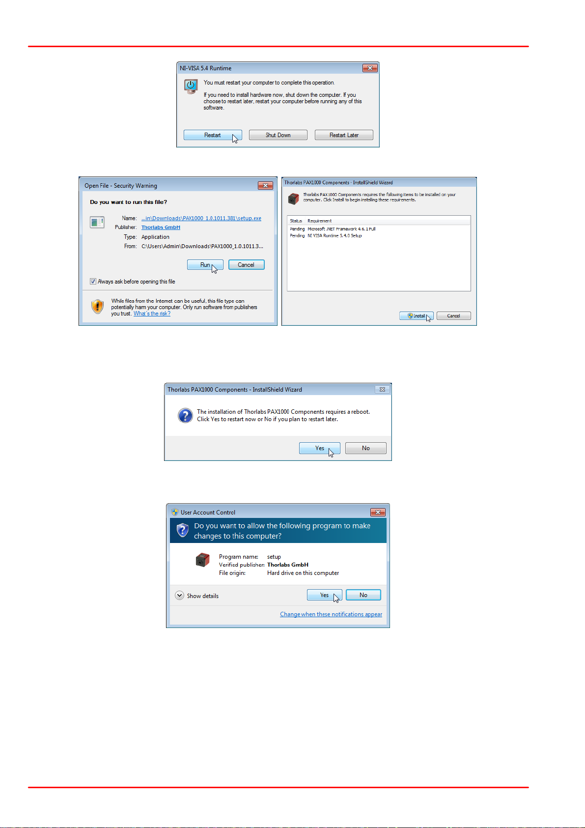
Download the software package to your computer, unzip it and execute the setup.exe:

2 Getting Started

Click 'Install' to proceed. Windows Security might require your confirmation to install the software, depending on the security level settings - please hit the appropriate button:

The installer starts the NI-VISA 5.4.0 installation. This will take some minutes and usually require a reboot.

Click 'Next' to continue. In the subsequent dialog windows, follow the instructions. Accepting the proposed settings is recommended..

If you are prompted to restart your computer, please do so to avoid installation issues.

PAX1000

After restarting the computer, the installer automatically resumes the installation process:

As a next step, the Microsoft .NET Framework will be installed. This installation procedure may take several minutes, please do not interrupt the installation process. When you are prompted again to restart your computer, please do so to avoid installation issues.

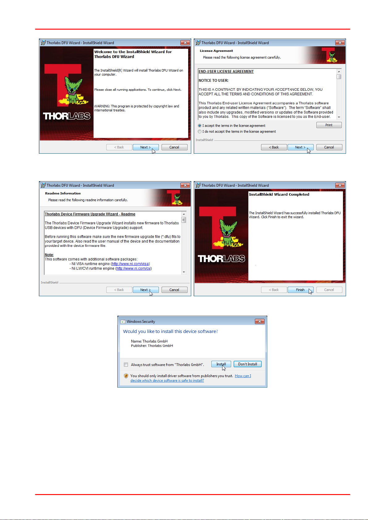
After restarting the computer, the installer automatically resumes the installation process and installs the Thorlabs DFU Wizard:

2 Getting Started

Click 'Next' to continue. In the subsequent dialog windows, follow the instructions. Accepting the proposed settings is recommended.

As a next step, the installer continues with installation of the PAX1000 software:

PAX1000

Click 'Next' to continue. In the subsequent dialog windows, follow the instructions. Accepting the proposed settings is recommended.

The Readme screen contains important information, please read it carefully. Then click 'Next'.

Click 'Finish' to finalize the installation of the software package.

2 Getting Started

2.6 First Steps

Mount your PAX1000 to the optical setup.

Note

Do not connect the PAX1000 to the PC prior to software installation! Please make sure that the installation was carried out completely, including the reboot requests. This is essential for a proper operation.

Power supplied via the USB2.0 port (max. 500 mA) is sufficient for waveplate rotation speeds up to 100 Hz. For faster measurements, please use in addition the supplied DS15 wall plug adapter.

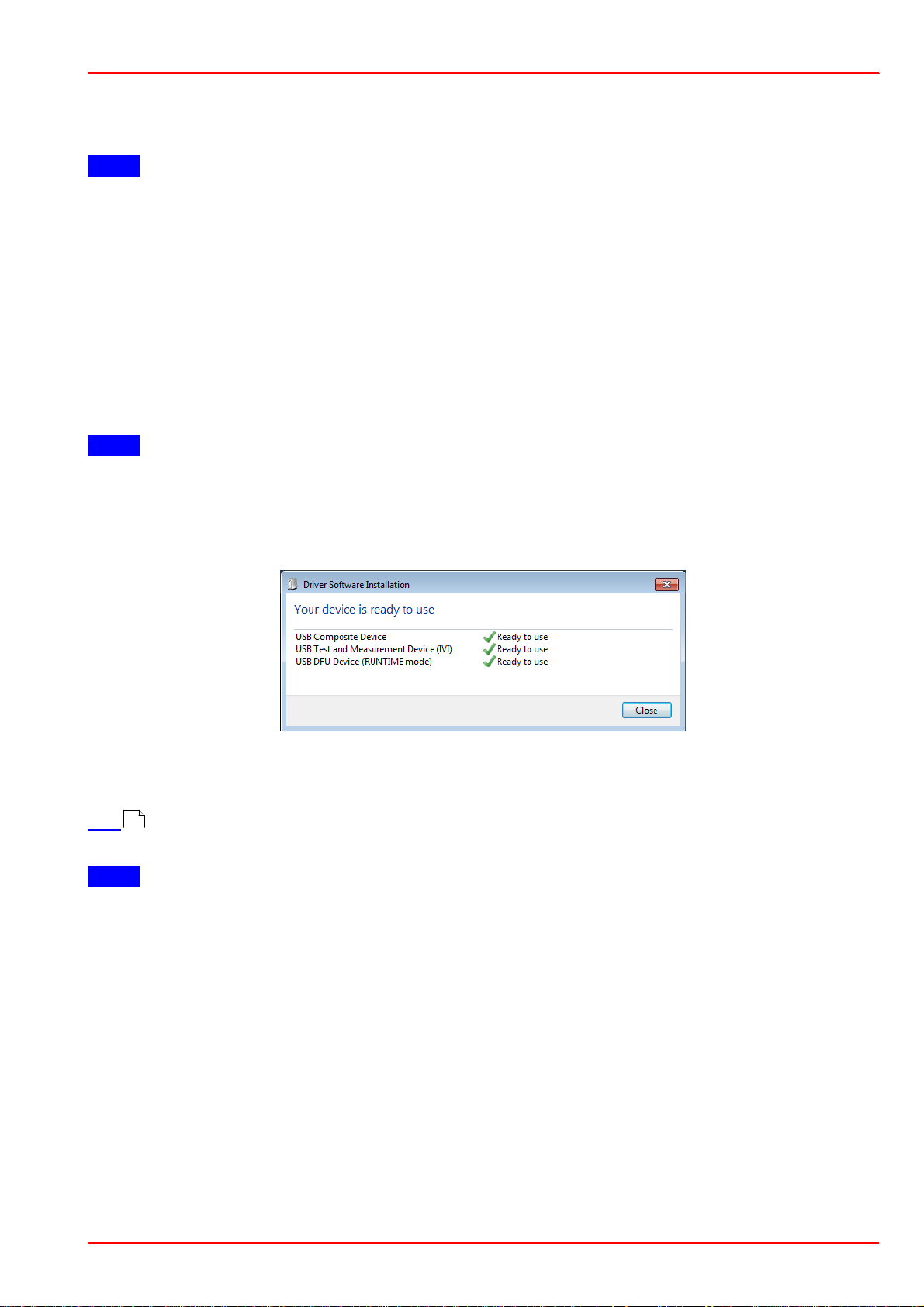
Connect the PAX1000 using the supplied USB2.0 cable to your computer. After connection of PAX1000xxx to your PC, the green LED on the back of the PAX1000xxx

lights up green and blinks during the booting phase of the device. Please take into account an initial warm up time of the PAX1000xxx.

Note

The supplied USB cable is certified for use with the PAX1000. The use of other and / or longer cables may lead to degradation of performance, data loss or even malfunction of the PAX1000.

A pop-up window confirms the PAX1000 is recognized by the computer, and it shows the installation status of the appropriate driver software.

It is recommended to skip the search for driver software in Windows Update, because no drivers will be found there and the installation process will consume longer time.

After the driver software was installed successfully, click to PAX1000 icon on your desktop. The

GUI (Graphic User Interface) comes up, scans the USB for installed devices and connects

automatically the recognized PAX1000.

Note

Up to five PAX1000 instruments can be connected at a time and displayed in a single software instance. If more that one PAX1000 is connected and recognized, the software will connect to the first recognized device any time the software is started.

PAX1000

3 Graphical User Interface (GUI)

3.1 General

Prior to explaining the GUI in detail, there are some general comments to make about the interactions between the PAX1000 hardware and the control software. Please read these comments carefully as this information is important to understanding the functionality.

The PAX1000 calculates the polarization parameters (power, degree of polarization and the three normalized Stokes vectors) in its firmware. These 5 parameters are transferred as a data set to the GUI via the USB connection.

Note

It is important to establish the USB connection prior to starting the software. Only this way the correct drivers can be installed and the PAX1000 can be recognized.

When the GUI starts for the first time, factory default settings for the GUI and default settings for the recognized PAX1000 are applied.

Upon exit, the software automatically saves the most recent workspace to an XML-type file that is located at

C:\Users\[user name]\AppData\Local\Thorlabs\PAX1000

This file contains

· the recent GUI appearance

· all measurement settings

· all PAX1000 devices that ever were connected, with their individual settings

This file is automatically updated any time the GUI is closed by the user. Please see section

Menu File for detailed information about the workspace.

Note

When powered via USB, a 50 to 100 Hz sample rate can be set. With connected external power supply, it can be set between 50 and 400 Hz.

3 Graphical User Interface (GUI)

3.2 GUI Overview

The GUI consists of a Tool Bar , several Ribbons , selectable Views (e.g. and ) and the Status Bar ( ). The ribbons can be minimized and restored using the small icon

to the right of the Thorlabs logo. Click to an area of the screenshot below to be directed to the appropriate section for detailed information.

Functions in View panels

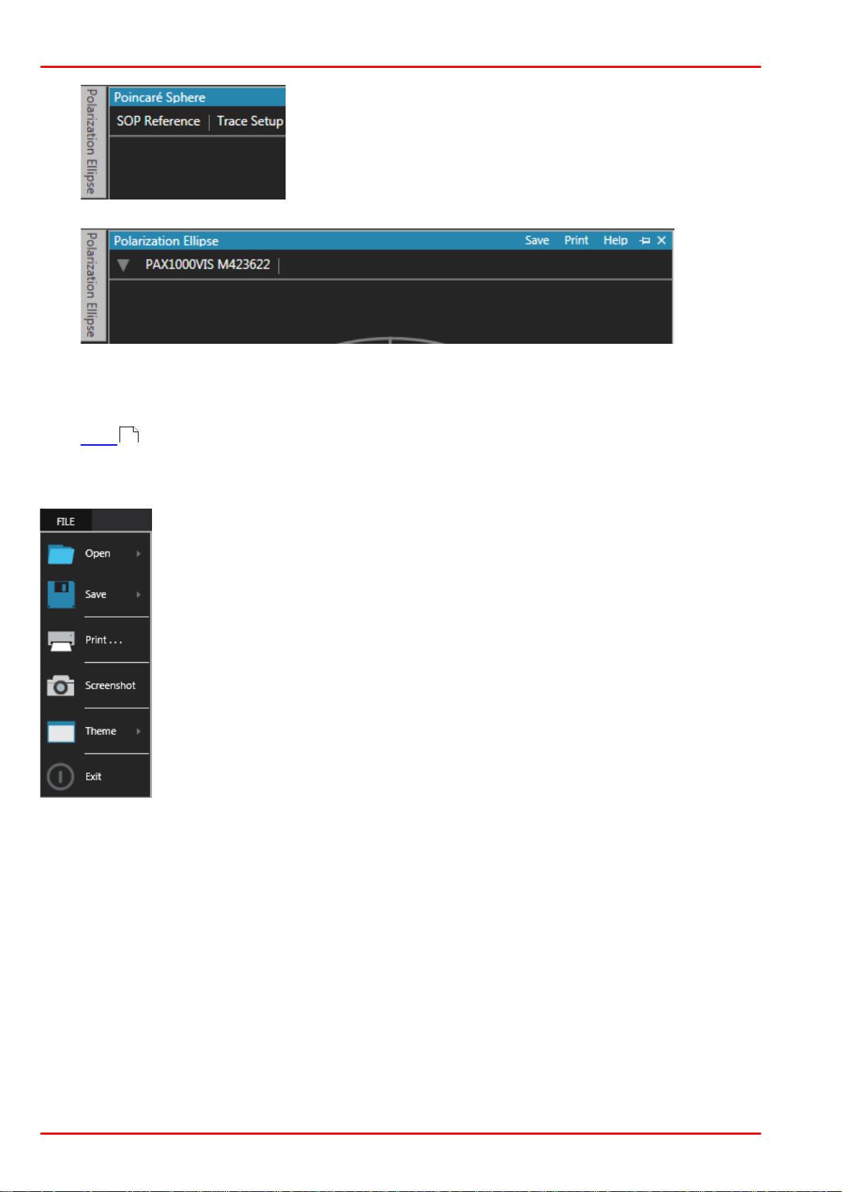
Each View panel has a header with five options:

· Save opens a dialog to save the content of the appropriate panel as a JPG, PNG or BMP image file.

· Print creates a screenshot of the appropriate panel in order to print it out to any installed system printer.

· Help opens the appropriate section in the PAX1000 software online help.

· The Pin allows to temporarily unpin the appropriate view from the GUI. Click the pin

and the Polarization Ellipse view collapses and appears like a bookmark on the left, while the other active view (here: Poincaré Sphere) is expanded over the entire GUI:

PAX1000

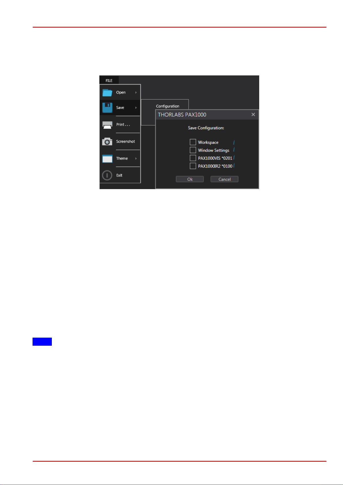
Open / Save Here you can open or save either a configuration or a measurement results file. For a detailed explanation, please see below.

Print... opens a new window with a screenshot of the actual GUI. This screenshot can be sent to any of your system printers, including PDF driver.

Screenshot creates a screenshot of the actual GUI and opens a dialog for saving this screenshot as JPG, PNG or BMP file.

Theme allows to toggle between a light or dark design of the GUI.

Exit closes the application. You can use the X icon in the upper right corner of

the GUI as well.

To recover the collapsed view, click to the bookmark and then the pin:

The collapsed view is recovered. As all active views share the GUI area, the pin/unpin function is helpful to keep the GUI clearly arranged and ensure a quick access to desired or often used view panels.

· The X in upper right corner allows to close the active view. They can be recalled in the

View menu by clicking the appropriate icon.

3.3 Menu File

3 Graphical User Interface (GUI)

Save Configuration

This option allows the setup of the GUI and/or the connected PAX1000 polarimeters to be saved. The saved configuration can be loaded later for use in future experiments, or with a different optical setup, or copied to and loaded into the software running on a different computer.

A configuration is an XML file, that may contain a selectable set of information and that is saved by default to ["My Documents"]\Thorlabs\PAX1000.

From the list in the Save Configuration dialog you can select:

· Workspace saves the configuration of the GUI view, i.e., which sub-panels are displayed, how they are located and sized. Example: If the GUI displays only the Scope, with a single diagram expanded, selecting Workspace will save this view.

· Window Settings saves the size, position and color theme of the GUI main window. Example: You are using two monitors in extended mode, and you the GUI was placed to the extension monitor with a certain size. Using the Window Settings, this arrangement will be saved.

· PAX1000xxx saves:

- Device settings and device information of the connected PAX1000.

- All actual settings of the Measurement Value Table, Polarization Ellipse, Poincaré

Sphere, Scope Mode and ER Measurement.

After selecting any of above options, a dialog opens to save the configuration file.

Note

Please assign an appropriate file name that tells you about the file content, because you can load afterwards just the entire configuration file, without any option to select workspace, window setting or device setting!

PAX1000

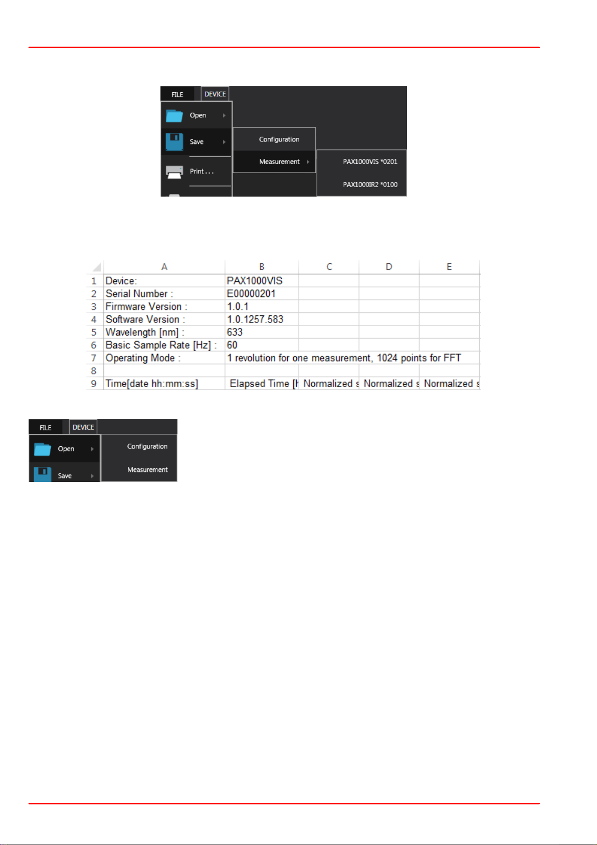
Save Measurement

The Measurement file is an CSV file that contains:

· Device settings and device information of the PAX1000 that was used for measurement.

· The most recent 1000 measurement results with time stamp.

Open

Here you can open a previously save configuration or a measurement results file.

3 Graphical User Interface (GUI)

3.4 Menu Device

Scan USB

Use this button to rescan all USB Ports in the case the connection was interrupted or an additional PAX1000 was connected during the session.

Note The PAX1000 software is able to connect up to five PAX1000 device per session, see

also Multiple Devices .

Add Virtual Device

Virtual devices can be used to test the software features without a PAX1000 hardware

connected, for example for evaluation purposes.

Devices & Measurements

A dialog opens that shows presently connected PAX1000 instruments and opened long-term measurement files. This way, an instrument can be disconnected and/or a measurement can be closed - just click on the entry.

Device Settings (Polarimeter)

This dialog lists the PAX1000 device information (read-only) and adjustable settings (within framed boxes). The icon in the header shows information about connected devices and loaded measurements and allows a selection.

Device Information

Model version, serial number, firmware version and external power supply status.

Settings

The Basic Sample rate is based on the rotation speed of the waveplate, while the Operating Mode defines measurement averaging and resolution. Please see section PAX1000 Set-

tings for detailed explanations of the parameters Basic

Sample, Sample Rate and Operating Mode.

Wavelength: Enter the operating wavelength to the best known accuracy. This is mandatory for correct measurements. The allowed value range is shown when hovering the mouse over the icon.

Power Range: The PAX1000 has a large input power dynamic range of 70 dB. To achieve a high measurement accuracy, a switchable gain amplifier is used. Each gain value corresponds

PAX1000

to a certain maximum input power. By default, the gain is switched automatically (box "Auto Power Range" is checked). In particular cases it might be useful to fix the power range - uncheck the box and set the power range then manually.

Device Color: Select a color for the selected PAX1000 instrument. This color will be used for Polarization Ellipse and Poincaré Sphere display of the measurement data. For each connected and active PAX1000 a different color is assigned that can be changed individually.

Button Default

This button resets the device settings of the selected PAX1000 to default:

· Operating wavelength depending on the device type: PAX1000VIS: 633 nm PAX1000IR1: 980 nm PAX1000IR2: 1550 nm

· Basic Sample Rate to 60 Hz

· Operating Mode to 1 (1024 pts FFT)

· Power Ranging to Auto

· Device Color to Blue

· Power Unit to dBm.

Device Settings (Measurement)

This dialog lists the settings of the PAX1000 device when the loaded measurement was executed. Only the settings within the framed boxes can be changed, these are Device Color and Power Unit.

Reset All

Resets both the GUI and the active PAX1000 settings to default: The GUI shows the ribbon device with the Polarization Ellipse and the Poincaré Sphere

pane, while the PAX1000 device settings are reset to factory defaults .

Pause / Run

This toggle icon allows to pause and resume the current data acquisition from the PAX1000 with the displayed below serial number.

3 Graphical User Interface (GUI)

3.5 Menu View

Click to an icon in the above shown screenshot to view the appropriate manual section. Reset Layout

This button resets only the GUI layout:

· Polarization ellipse with numerical values for azimuth and ellipticity

· Poincaré sphere in default view (H (horizontal SOP) in front); clears all traces, clears

marker circle

There is no impact on device settings (e.g., wavelength) and measurement settings (e.g., SOP references remain).

3.6 Menu Tools

Click to an icon in the above shown screenshot to view the appropriate manual section.

3.7 Menu Help

Troubleshooting

Contact Technical Support opens Thorlabs' web site

with the list of world-wide contacts. Save Logfile: This file logs the most recent 5 software

sessions. It might be helpful to attach this file to a Tech Support request.

System Info: Displays the Windows System Information about the used PC.

PAX1000 Help

Click this button to open the online help. When pressing the F1 key, the online help opens with the section of the currently active view (context sensitive help).

PAX1000

Product License

Opens the License.rtf file.

About Thorlabs PAX1000

Displays information about the current PAX1000 software.

3.8 Status Bar

By default, the status bar displays only the actual date and time:

It is used to indicate common errors as well as information about long-term measurement (LtM) progress and errors that were observed during the current LtM session:

Please see section Error Messages for detailed explanations.

4 PAX1000 Settings

Prior to explain PAX1000 Setting, lets shortly recapitulate the measurement procedure that is discussed in detail in section

Rotating Waveplate Technique :

The PAX1000 uses a rotating quarter waveplate for polarization analysis. A half turn of the waveplate is sufficient to uniquely determine the state of polarization. The parameter Basic Sample rate is always related to this half-turn. The photo current measured during this half turn is analyzed by a Fast Fourier Transformation (FFT). By default, the FFT "splits" the data into 512 measurement points (ADC values). In order to increase the measurement accuracy:

· the number of FFT points can be set to 1024 or 2048;

· the FFT can be carried out over a full turn or over 2 full turns

of the waveplate. The parameter Operating Mode reflects that:

For example, the operating mode "1/2 (512 pts FFT)" means, that the data for calculation are collected per 1/2 revolution of the waveplate (number of basic periods = 1/2), and the FFT is

carried out on 512 points (number of AD converter values) within this half turn. So, the resulting sample rate or measurement speed can be written

Mathematically, the number of points used for FFT does not impact the measurement speed. The more FFT points are used, the higher the measurement accuracy, but the higher is also the workload of the microcontroller. Particularly, at high measurement speed and high FFT resolution, measurement data might be not captured because the microcontroller is busy with FFT calculation.

Recommendations

For fast measurements use a high basic sample rate, a small operating mode value and fewer FFT calculation points. At this setting, measurement accuracy might be impacted.

When measuring an optical signal at low power power or with significant noise, decrease the basic sample rate, increase the operating mode and use more FFT points.

Note

When the PAX1000 is powered via USB only, the Basic Sample Rate can be set between 50 and 100 Hz. With external power supply, the maximum Basic Sample Rate is 400 Hz.

PAX1000

5 Operating Instruction

5.1 Alignment Assistance

For accurate measurements, it is essential to align the incident beam so that it is centered in the input aperture and is normally incident on the rotating l/4 waveplate.

The beam centering is particularly important in the case of large incident beam diameters, close to the aperture diameter ( Ø 3.0 mm). In such cases the correct centering is essential to avoid beam cutting and reflections from the inner surface of the hollow shaft that holds the waveplate. The beam centering can be achieved by using the protection cap with engraved cross-hair (PAX1000VIS) or with a viewing target (PAX1000IR1 and ~IR2).

The angular alignment is critical for another reason: As explained in the section Rotating Wave-

plate Technique , the photo current is analyzed by a Fast Fourier Transformation and ideally

consists only of even-numbered components (harmonics). If the beam hits the waveplate not exactly perpendicular, unwanted odd-numbered harmonics will appear in the photo current. The same happens, if the incident beam consists reflected from the inner surface of the hollow shaft light components. These unwanted components have a significant impact on the measurement accuracy. The Alignment Assistance tool can be used to align the beam, which will minimize the contribution from unwanted components.

Click the icon in the Tools ribbon. A new screen comes up.

The Alignment graph shows the fraction of wanted components in the photo current. The green portion of the scale defines the range of acceptable alignment values. Click the Start Alignment button.

Adjust the alignment of the beam with respect the PAX1000 beam. When the best alignment is achieved, click Stop Alignment and close the window.

5.2 PAX1000 Measurements

Note

5 Operating Instruction

Prior to starting a measurement, please make sure that the device settings are entered prop-

erly. Particularly, the correct wavelength and power ranging (preferred setting: Auto Range) are essential for accurate measurement results.

The PAX1000 software provides several polarization measurement views that can be called from the View ribbon. If this ribbon is hidden, please click the small arrow next to the Thorlabs logo (marked yellow):

These views are described in detail in the subsequent sections:

· Measurement Value Table

· Polarization Ellipse

· Poincaré Sphere

· Scope Mode

· Long Term Measurement

· Extinction Ratio Measurement

The Reset Layout button resets the GUI layout to:

· Polarization ellipse with numerical values for azimuth and ellipticity

· Poincaré sphere in default view H (horizontal SOP) in front; clears all traces, clears

marker circle

There is no impact on device settings (e.g., wavelength) and measurement settings (e.g., SOP references remain).

PAX1000

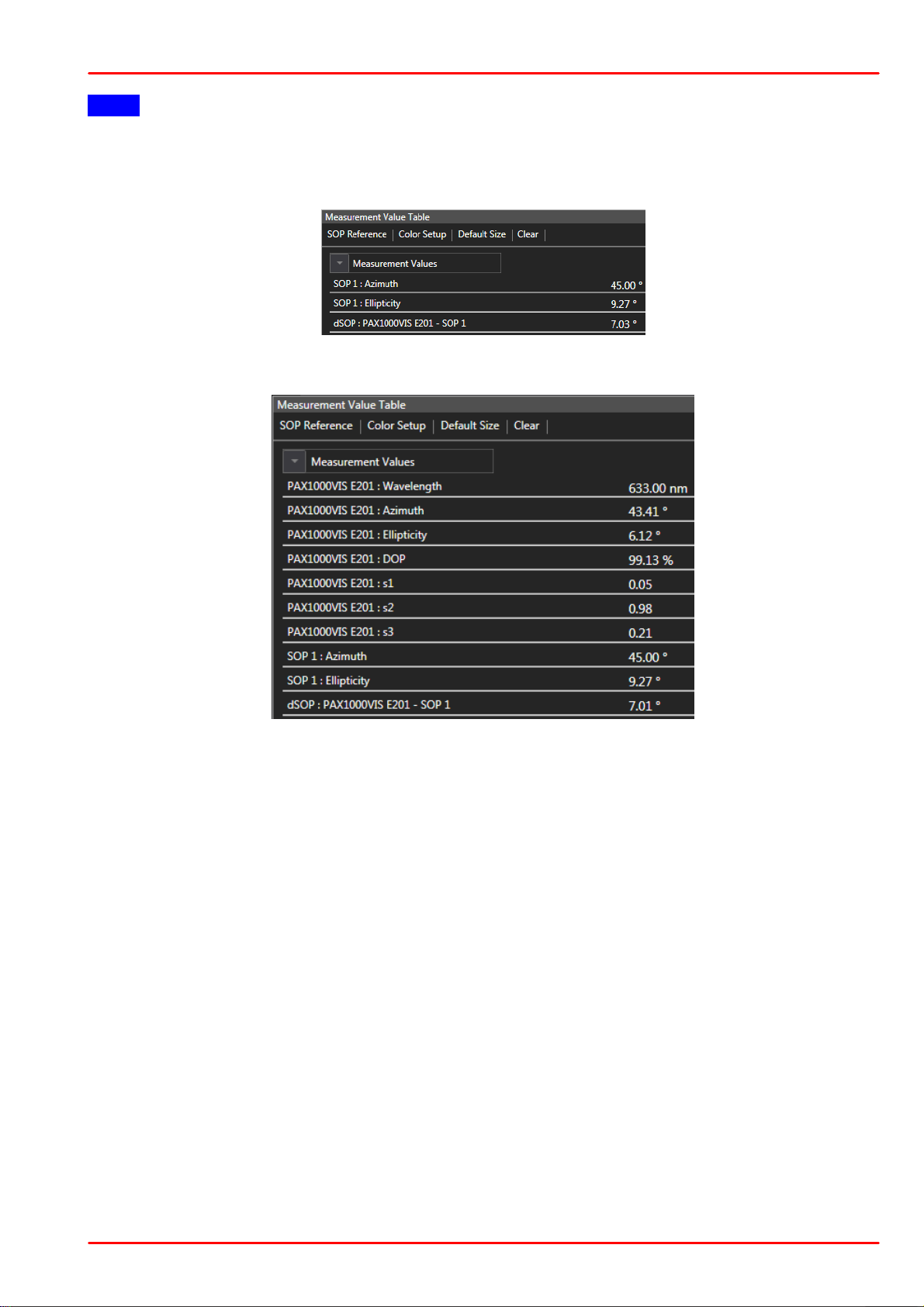
5.2.1 Measurement Value Table

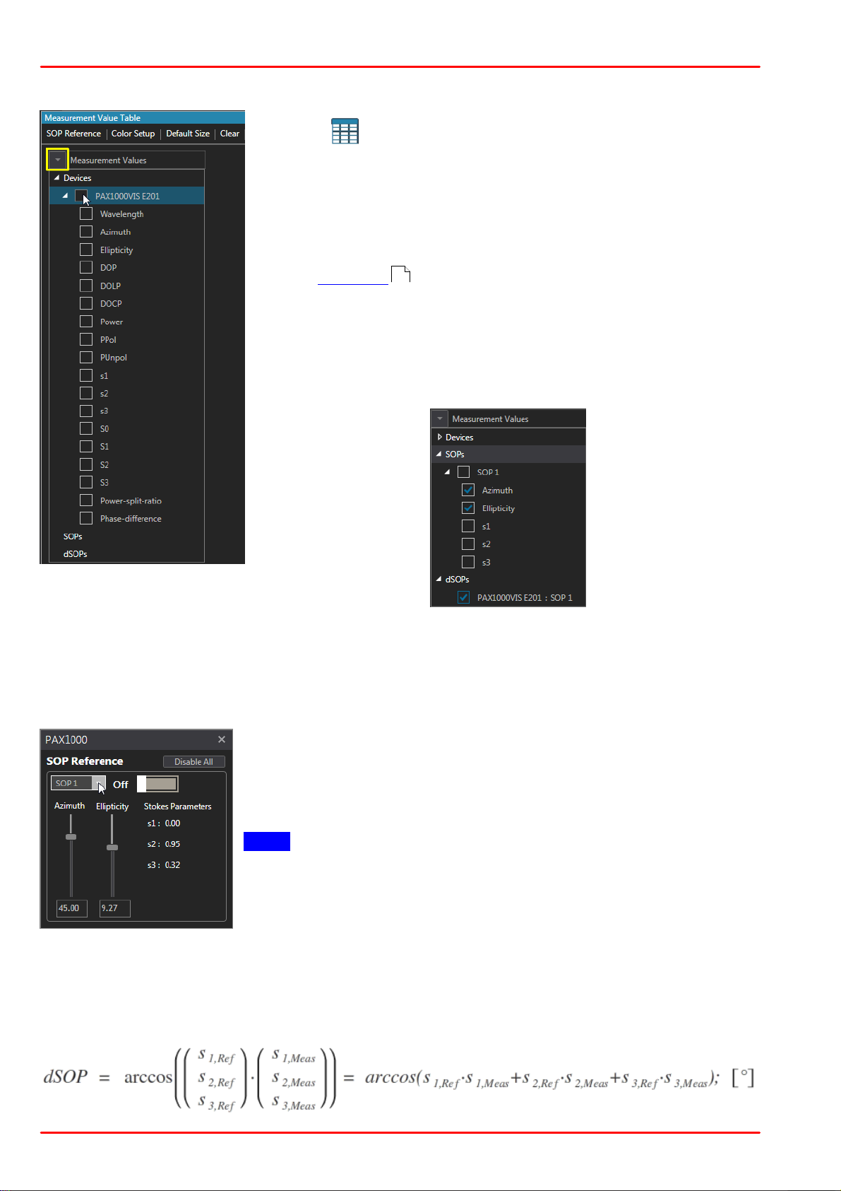
Click the icon to show the Measurement Value Table. It displays a selectable number of polarization parameters numerically in a list. Click the drop-down arrow (marked yellow) to expand the list and select the desired parameters. When checking the box of the active PAX1000, all parameters will be enabled, with the possibility to disable any of them.

For detailed explanation of the polarization parameters, please see the Appendix .

If more than one PAX1000 is connected and active, this selection can be made for each of these devices.

If at least one SOP Reference is enabled, you can select the polarization parameters of the reference that shall be displayed numerically, as well as the dSOP:

A SOP reference is a certain, user-configurable state of polarization that can be used as a reference point. In combination with the dSOP parameter, this allows to measure the polarization shift of the actual state of polarization from the reference point.

Up to 20 reference SOPs can be defined. Click to the menu item SOP Reference. A dialog opens:

Select from the drop-down menu one of SOP 1 to SOP 20. Define the azimuth and ellipticity for this reference point, either by

using the slider or by entering the desired value numerically. The software automatically calculates the appropriate normalized Stokes vectors.

Note The Stokes vectors cannot be entered by the user.

Set the switch from Off to On to enable the actual SOP reference. The Disable All button disables all SOP references at once.

dSOP

dSOP is the difference between the actual measured SOP and a SOP reference, in degree. This is the angle between the two polarization vectors on the Poincaré sphere. Using the normalized Stokes vectors, this can be written mathematically as:

5 Operating Instruction

Note

Above formula takes into account that the normalized Stokes vectors with an absolute value =1 are used for calculation.

The dSOPs will be displayed in Measurement Value Table this way:

By clicking to the area outside the parameter selection window, the parameter selection panel

closes and in the GUI will be displayed the table with measurement results:

PAX1000

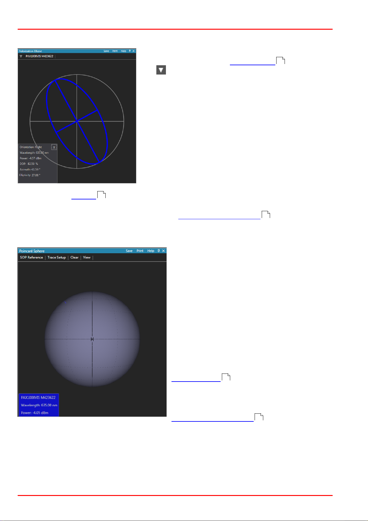
5.2.2 Polarization Ellipse

In this view, the polarization ellipse is displayed. The ellipse color depends on the device setting .

The icon in the left upper corner allows to select one of the connected polarimeters for display.

Below the ellipse, a box with numerical parameters is shown. The first four parameters

- orientation (handedness)

- wavelength

- total power

- DOP (degree of polarization) are shown at any time.

By clicking to the grey area, the display of the additional parameters can be changed:

- azimuth and ellipticity, or

- power split ratio and phase difference, or

- the 3 normalized Stokes vectors s1, s2 and s3.

Please see the Tutorial for detailed information on these parameters. The numerical para-

meters can be hidden (X); then the small i icon will restore them. For functions in the blue header line, please see Functions in View panels .

5.2.3 Poincaré Sphere

The default view of the Poincaré sphere is shown in the screenshot.

Viewing options

· Click the colored box to show the current SOP in front. If you have more than one PAX1000 connected, the click shows the current SOP of the selected device.

· Hold the left mouse button and drag to rotate the sphere.

· Scroll the mouse wheel or press + (-) to zoom the view.

· To move the sphere, press A (left), D (right), W (up) or S (down).

· Press Ctrl and left mouse button to create a

SOP reference .

· Press Ctrl, hold down right mouse button and drag to create a circular marker on the sphere.

For functions in the blue header line, please see

Functions in View panels .

Menu SOP References

Up to 20 reference SOPs can be defined.

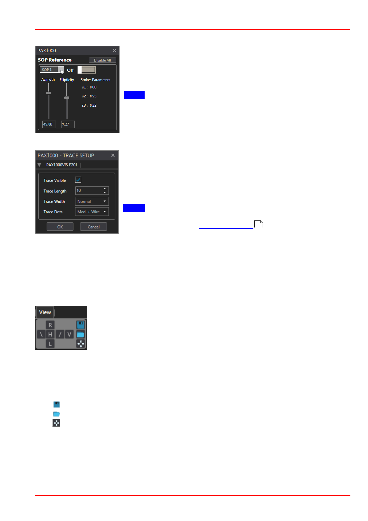
Click to the menu item SOP Reference. A dialog opens:

Select from the drop-down menu one of SOP 1 to SOP 20. Define the azimuth and ellipticity for this reference point, either by

using the slider or by entering the desired value numerically. The software automatically calculates the appropriate normalized Stokes vectors.

Note The Stokes vectors cannot be entered by the user.

Set the switch from Off to On to enable the actual SOP reference. The Disable All button disables all SOP references at once.

Menu Trace Setup

In this menu you setup the SOP trace on the Poincaré sphere. When enabled, each SOP measurement point is added to the trace until the selected trace length is reached. The dwell time of a trace this way depends on the trace length and the measurement speed.

Trace Visible enables/disables the trace display. Trace Length Values between 1 and 50,000 can be entered.

Note : The maximum trace length is limited for memory load reas-

ons and it is available only in case of a single device is connected. Please refer to section Multiple Devices .

Trace Width can be selected to thin, normal and bold.

Trace Dots Select the shape of the trace:

- small, medium or large dots only

- small, medium or large wired dots, or - wire only.

5 Operating Instruction

Click OK to apply settings and close the panel.

Menu Clear Clears the trace. SOP references remain. Menu View

Adjust, how you want to look at the Poincaré sphere. H and V rotate the sphere to bring the equatorial points corresponding to the

linear horizontal and vertical polarizations, respectively, to the front.brings the horizontal resp. vertical point (linear horizontal/vertical polarization) on the

sphere's equator to the front. R and L rotate the sphere to bring the polar points corresponding to the right or left handed circular polarizations, respectively, to the front. Finally, \ and / rotate the sphere to bring the points corresponding to an azimuth of -45° and +45°, respectively, to the front.

The 3 buttons to the right provide the following functions:

· Saves the current Poincaré sphere orientation and zoom factor as user view..

· Recalls the saved user view.

· Resets the zoom to default, all other view settings are not impacted.

PAX1000

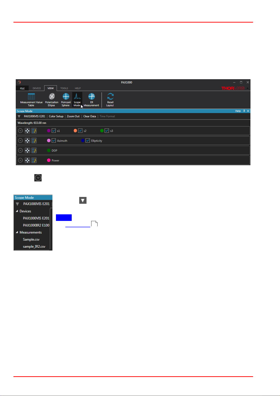
5.2.4 Scope Mode

In Scope Mode, the 1000 most recently measured polarization parameters are shown plotted to a graph. The graph can be continuously updated as values are acquired. The data logging

· starts with the connection of a PAX1000 device

· restarts after pressing the Clear Data button.

Select from the View ribbon the item Scope Mode.

In the initial view shows four parameter groups, with the display of the scope graphs collapsed. Use the icon to show the desired diagram.

Select Data Source

Click the icon and expand Devices and/or Measurements to select a data source.

Note In order to select a saved measurement, it must be opened first from

the File menu !

Color Setup This menu assigns the color to the individual graphs. Select your preferred color. Clear Data deletes the accumulated measurement value and restarts the display. The time axis

is then zoomed until the maximum of 1000 measurement values is reached. After reaching 1000 samples, the diagram shows the most recent 1000 samples, i.e., with each new sample, the oldest is discarded, and the times axis shifts.

Time Format: If a measurement is loaded and selected for display, the time format can be toggled between time stamp and elapsed time. For running measurements (a PAX1000 is selected), only the time stamp is used.

5 Operating Instruction

Hover the mouse pointer over the diagram area ...

... and scroll the mouse wheel

Diagram Options

Each of the four diagrams can be modified for the best view. Additionally, for the first two diagrams (normalized Stokes vectors; ellipticity/azimuth) you can select the parameters to be displayed. The diagram options are explained below using the example of the Stokes vectors diagram with a saved measurement loaded from a file.

Toggle the diagram view between expanded and collapsed. Expand the diagram over the entire GUI window by hiding the other 3 charts. Set the upper and lower limits of the Y scale:

Set the desired limits either by entering numerically or using the up/down arrows.

Click OK to apply changes. Click Reset to restore the scale limit to the maximum in accordance with the actual parameter.

Zoom and Pan

Place the mouse pointer to the point in the diagram that you want to zoom in. A yellow marker appears. Scroll the mouse wheel and the diagram will be zoomed in around the moose pointer in both the Y and time scale directions:

Note

The yellow marker appears instantly when hovering the mouse over the diagram only if a loaded measurement is displayed. In live mode, when the measurement of a PAX1000 is displayed, the yellow marker appears only after the mouse wheel was rotated. Then the display of the current measurement is paused and the diagram can be zoomed.

PAX1000

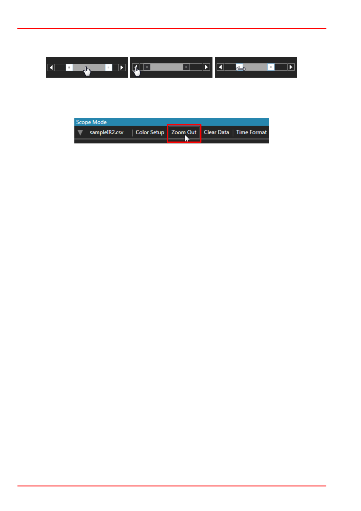
Pan Diagram

Zoom Diagram

Another way to zoom and pan the diagram is the use of the zoom-pan-sliders to the left and below the chart:

Using the Zoom Out button in the diagram header, you can instantly return to the full diagram view:

5.2.5 Long Term Measurement

The LTM buttons can be found in the Tools ribbon.

The long-term measurement tool records the following parameters:

· Stokes vectors S0, S1, S2 and S3 [mW]

· Normalized Stokes vectors s1, s2 and s3

· Azimuth [ ° ]

· Ellipticity [ ° ]

· Degree of polarization [ % ]

· Degree of linear polarization [ % ]

· Degree of circular polarization [ % ]

· Total power [ mW / dBm ]

· Polarized power [ mW / dBm ]

· Unpolarized power [ mW / dBm ]

· Power split ratio

· Phase difference

5 Operating Instruction

Each set of above listed parameters is provided with the exact time stamp (dd.mm.yyy hh:mm:ss) and the elapsed time with millisecond resolution (d.hh:mm:ss:msec). The recorded file format is *.csv and can be easily imported to Microsoft Excel. Alternatively, the data can be saved as a *.txt file.

5.2.5.1 Settings

Prior to starting a long-term measurement, open the LTM Settings panel and enter the measurement conditions.

1. Select a folder, the file name and file format.

2. Select the sampling frequency. Options:

· Set the sample acquisition time interval to a value from 50 ms to 60 s in increments of 1 ms.

· Specify which measurements to record to file, with a value of 1 recording every measurement and a maximum value of 10000 recording every 10000th measurement.

3. Select the Stop criteria:

· after reaching a file size between 0.1 and 1000 MB

· after reaching a record time 10 sec and 365 days

23:59:59 hours

· after recording 1 to 10000 measurement data sets

PAX1000

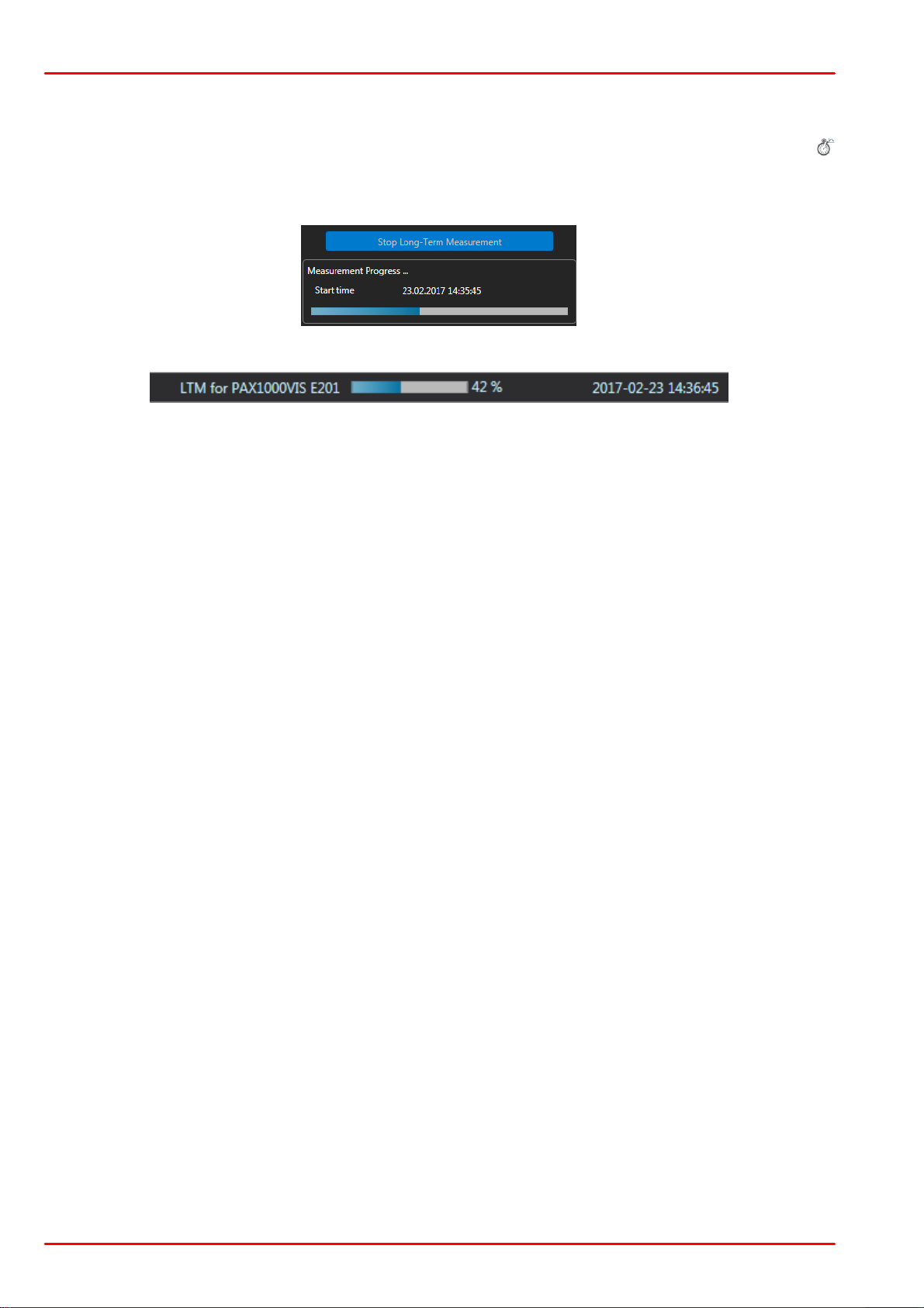
5.2.5.2 Measurement

After completing the desired settings for your long-term measurement, the recording can be started by pressing the Start Long-Term Measurement button in the settings panel or the

button in the ribbon Tools.

The measurement progress is shown in the settings panel

and in the status bar on the bottom of the GUI:

5 Operating Instruction

5.2.6 Extinction Ratio Measurement

The PAX1000 allows the measurement of the Extinction Ratio (ER) of polarization maintaining fibers (PMF). Please see the section Extinction Ratio Measurement on PM Fibers for theory and basics.

Measurement Setup

For correct ER measurements, a linearly polarized light source is mandatory. This can be a pigtailed laser diode with a PMF output fiber, or a free space laser combined with a fiber coupler and a Thorlabs Fiber-To-Fiber U-Bench or a manual fiber polarization controller.

The DOP (degree of polarization) of the light source should be as close to 100% as possible. Also, the operating wavelength must be well known, and the optical power must not exceed the specification of the PAX1000.

It is important to couple the linearly polarized light parallel to the slow axis of the fiber under test.

The output of the fiber under test is connected to the PAX1000 using the supplied fiber collimator with the SM1 adapter.

Note

The F240FC-x collimator is designed for FC/PC connectors. If your fiber under test has an angled connector (FC/APC), please purchase a Thorlabs F240APC-x collimator. "x" stands for the operating wavelength range of the anti-reflective coating and must match with your PAX1000 and the operating wavelength of your setup.

The fiber under test must be dynamically stressed while the ER measurement is performed. Below, an example of an ER Measurement Setup is shown:

The optical test signal is generated by a DFB laser diode. Its output is connected to a Thorlabs GmbH PL100S deterministic polarization controller. The PMF under test (fiber with blue jacket)

PAX1000

is connected to the output of the polarization controller and the input of the polarimeter (the discontinued polarimeter model PAX5720 is shown).

The fiber is heated when the filament bulb in the center of the looped fiber is turned on, which stresses the fiber. However, the stress can also be applied mechanically, e.g. by pulling the fiber manually.

Note

The mentioned above stress methods are applicable only to PMF without tubing! During measurement, i.e., when the fiber is stressed, the PMF output SOP (State of Polariza-

tion) describes a circle on the Poincaré Sphere. For reliable ER Measurement results, at least a full circle must be drawn (i.e. the stress must vary enough during the test to result in this minimum change in polarization state).

5 Operating Instruction

5.2.6.1 ER Measurement Wizard

The ER Measurement Wizard guides you through the preparation and measurement step by step.

Note

If you are already familiar with this measurement, you may use the ER Measurement tool

directly. Open the ER Measurement Wizard from the Tools menu.

The Start Window summarizes how to set up the measurement. Additional details are given in the previous section .

If necessary, select the PAX1000 for measurement, then click .

PAX1000

Enter the operating wavelength of your light source and select the desired measurement time. Select the option Stop on Circle Completed, which will terminate the measurement as soon

as the SOP change reached a full circle. When done, click .

The current SOP is displayed on the Poincaré Sphere. Click to proceed.

5 Operating Instruction

Save the numeric test results and the Poincaré Sphere screenshot to a PDF file.

Return to the previous window.

Close the ER Measurement Wizard and return to the PAX1000 GUI.

After finishing the measurement, above final screen appears.

Please see the Tutorial in the appendix for detailed explanation of the options Compensate El-

lipticity and Compensate DOP .

Please see next section for detailed explanations of the numerical results. If a warning or an error message appears, please see section Troubleshooting for possible

75 76

reasons and solution proposals.

PAX1000

5.2.6.2 ER Measurement Tool

The tool ER Measurement allows the easy measurement the Extinction Ratio of PM fibers. During the measurement, the fiber must change enough to cause at least a change of polarization that describes a circle on the Poincaré Sphere: The smaller the circle diameter, the higher the ER value.

1. Prepare your setup . Ensure a correct coupling of the light signal into the fiber - the dot on

the Poincaré Sphere representing the SOP out of the fiber should lay as close as possible to the H mark. Azimuthal deviations from the Horizontal polarization are not critical, whereas a position towards the poles indicates an ellipticity that is caused by miscoupling of the light into the fiber under test.

2. Start the ER Measurement tool from the appropriate button in the view ribbon:

3. Enter the operating wavelength of your light source.

Note : An exact wavelength value is essential for minimum measurement errors.

4. Select the measurement time between 3 and 10 s. During measurement, the fiber stress must cause at least a full circle on the Poincaré Sphere. The higher the stress applied to the fiber, the shorter the time to achieve this. You may select for a first try the maximum time of 10 s and check the box Stop on Circle Completed.

5. Start the fiber stress and the ER measurement.

5 Operating Instruction

Total Points

This is the total number of measured points (SOPs).

Used Points

The software has an internal algorithm that excludes points located too close to each other from the total number of measured points. The remaining points are used for circle approximation and subsequently for ER calculation.

Extinction Ratio

Measurement result is displayed with respect to the state of the check boxes Compensate Ellipticity and Compensate DOP. For detailed explanations and examples of these compensations, please see section Cor-

rection of the Polarimeter ER Measurements in the Tutorial.

Center Azimuth

Azimuth angle of the center of the calculated circle.

Center Ellipticity

Ellipticity angle of the center of the calculated circle.

Radius

Radius of the calculated circle in ° on the Poincaré Sphere.

Deviation

Standard deviation of the Used Points from the approximated circle.

6. After finishing the measurement, the GUI will display the measurement results:

7. The yellow circle represents the measured states of polarization, while the black circle is the approximation that is used for calculation of the ER.

Measurement Results

The box Measurement displays the parameters that were measured at the end of the ER Measurement.

The box ER Measurement Results displays several parameters:

If a warning or an error message appears, please see section Troubleshooting for possible reasons and solution proposals.

PAX1000

5.2.7 Virtual Device

A virtual PAX1000 can be connected. This is an easy way to evaluate the PAX1000 software without the hardware. This device is based on a PAX1000IR1 with its default settings . These

settings cannot be changed. The virtual device delivers random measurement values that can be used to test all measure-

ment functionality, except the ER measurement on PM fibers.

5.2.8 Multiple Devices

The PAX1000 software allows up to five PAX1000 devices, including live devices and measurement files, to be simultaneously connected. Connect the PAX1000. Open menu Devices & Measurements in the DEVICE ribbon - all connected and recognized PAX1000 devices are listed here, along with loaded measurement files.

Note

If you do not see the device that your want to connect, please make sure that the USB connection is made properly. Click Scan USB force recognition.

Each view of the GUI allows a selection of the device to be displayed from a drop-down menu:

In the Poincaré sphere view all connected devices are displayed at the same time:

5 Operating Instruction

Note

A total of 50,000 measurement values can be displayed on the Poincaré sphere. This limitation was set in order to save system resources. This limitation affects the maximum trace length. If more than one PAX1000 is connected, the maximum number of points that can be displayed on the Poincaré sphere, equal to the maximum trace length, will be shared:

1 PAX1000: max. 50,000 points 2 PAX1000: max. 25,000 points 3 PAX1000: max. 15,000 points 4 PAX1000: max. 12,500 points 5 PAX1000: max. 10,000 points

For any loaded measurement file, a maximum of 1000 most recent points will be displayed on the Poincaré sphere. However, in the Scope Mode, all measurement data of a loaded file will be displayed.

Please note also, that in the case of large trace lengths and multiple device operation, the software performance may degrade significantly, depending on the computer's resources.

PAX1000

Programming environment

Necessary files

C, C++, CVI

*.fp (function panel file; CVI IDE only) *.h (header file) *.lib (static library) *.dll (dynamic linked library)

.net wrapper dll

Visual Studio

*.h (header file) *.lib (static library) or .net wrapper dll

LabView

*.fp (function panel) and NI VISA instrument driver Beside that, LabVIEW driver vi's are provided with the *.llb con-

tainer file

6 Write Your Own Application

In order to write your own application, you need a specific instrument driver and some tools for use in different programming environments. The driver and tools are included in the installer package and cannot be found as separate files on the installation CD.

In this section the location of drivers and files, required for programming in different environments, are given for installation under Windows 7, Windows 8.1 and Windows 10 (32 and 64 bit)

Note

PAX1000 software and drivers contains 32 bit and 64 bit applications. In 32 bit systems, only the 32 bit components are installed to

C:\Program Files\…

In 64 bit systems the 64 bit components are being installed to

C:\Program Files\…

while 32 bit components can be found at

C:\Program Files (x86)\…

In the table below you will find a summary of what files you need for particular programming environments.

Note

All above environments require also the NI VISA instrument driver dll ! During NI-VISA Runtime installation, a system environment variable VXIPNPPATH for including

files is created. It contains the information where the drivers are installed to, usually to

C:\Program Files\IVI Foundation\VISA\WinNT\.

This is the reason, why after installation of a NI-VISA Runtime a system reboot is required: This environment variable is necessary for installation of the instrument driver software components.

In the next sections the location of above files is described in detail.

6 Write Your Own Application

6.1 32 Bit Operating Systems

Note

According to the VPP6 (Rev6.1) Standard the installation of the 32 bit VXIpnp driver includes both the WINNT and GWINNT frameworks.

VXIpnp Instrument driver:

C:\Program Files\IVI Foundation\VISA\WinNT\Bin\TLPAX_32.dll

Note

This instrument driver is required for all development environments!

Header file

C:\Program Files\IVI Foundation\VISA\WinNT\include\TLPAX.h

Static Library

C:\Program Files\IVI Foundation\VISA\WinNT\lib\msc\TLPAX_32.lib

Function Panel

C:\Program Files\IVI Foundation\VISA\WinNT\TLPAX\TLPAX.fp

Online Help for VXIpnp Instrument driver:

C:\Program Files\IVI Foundation\VISA\WinNT\TLPAX\Manual\TLPAX.html

NI LabVIEW driver (including an example VI)

The LabVIEW Driver is a 32 bit driver and compatible with 32bit NI-LabVIEW versions 8.5 and higher only.

C:\Program Files\National Instruments\LabVIEW xxxx\instr.lib\TLPAX… …\TLPAX.llb

(LabVIEW container file with driver vi's and an example. "LabVIEW xxxx" stands for actual LabVIEW installation folder.)

.net wrapper dll

C:\Program Files\Microsoft.NET\Primary Interop Assemblies… …\Thorlabs.PAX1000.Interop.dll

C:\Program Files\IVI Foundation\VISA\VisaCom\Primary Interop… …Assemblies\Thorlabs.PAX1000.Interop.dll

Example for C

Source file:

C:\Program Files\IVI Foundation\VISA\WinNT\TLPAX\Examples\CSample\… …sample.c

(C program how to communicate with a PAX1000 Series polarimeter)

Example for C#

Solution file:

C:\Program Files\IVI Foundation\VISA\WinNT\TLPAX\Examples… …\CSharp\Thorlabs.PAX_CSharp_Demo.sln

PAX1000

Project file:

C:\Program Files\IVI Foundation\VISA\WinNT\TLPAX\Examples… …\CSharp\Thorlabs.PAX_CSharp_Demo\Thorlabs.PAX_CSharp_Demo.csproj

Executable sample demo:

C:\Program Files\IVI Foundation\VISA\WinNT\TLPAX\Examples… …\CSharp\Thorlabs.PAX_CSharp_Demo\bin\Thorlabs.PAX_CSharp_Demo.exe

Example for LabView

Included in LabVIEW llb container.

6 Write Your Own Application

6.2 64 Bit Operating Systems

Note

According to the VPP6 (Rev6.1) Standard the installation of the 64 bit VXIpnp driver includes the WINNT, WIN64, GWINNT and GWIN64 frameworks. That means, that the 64 bit driver includes the 32 bit driver as well.

In case of a 64 bit operating system, 64bit drivers and applications are installed to

“C:\Program Files”

while the 32 bit files - to

“C:\Program Files (x86)”

Below are listed both installation locations, so far applicable.

VXIpnp Instrument driver:

C:\Program Files (x86)\IVI Foundation\VISA\WinNT\Bin\TLPAX_32.dll C:\Program Files\IVI Foundation\VISA\Win64\Bin\TLPAX_64.dll

Note

This instrument driver is required for all development environments!

Header file

C:\Program Files (x86)\IVI Foundation\VISA\WinNT\include\TLPAX.h C:\Program Files\IVI Foundation\VISA\Win64\include\TLPAX.h

Static Library

C:\Program Files (x86)\IVI Foundation\VISA\WinNT\lib\msc… …\TLPAX_32.lib

C:\Program Files\IVI Foundation\VISA\Win64\Lib_x64\msc\TLPAX_64.lib

Function Panel

C:\Program Files (x86)\IVI Foundation\VISA\WinNT\TLPAX\TLPAX.fp

Online Help for VXIpnp Instrument driver:

C:\Program Files (x86)\IVI Foundation\VISA\WinNT\TLPAX\Manual… …\TLPAX.html

NI LabVIEW driver (including an example VI)

The LabVIEW Driver supports 32bit and 64bit NI-LabVIEW2009 and higher. 32 bit NI-Labview version

C:\Program Files (x86)\National Instruments\LabVIEW xxxx\instr.lib… …\TLPAX\TLPAX.llb

64 bit NI-Labview version

C:\Program Files\National Instruments\LabVIEW xxxx\instr.lib… …\TLPAX\TLPAX.llb

(LabVIEW container file with driver vi's and an example. "LabVIEW xxxx" stands for actual LabVIEW installation folder.)

PAX1000

.net wrapper dll

C:\Program Files (x86)\Microsoft.NET\Primary Interop Assemblies… …\Thorlabs.PAX1000.interop.dll

C:\Program Files (x86)\IVI Foundation\VISA\VisaCom\… …Primary InteropAssemblies\Thorlabs.PAX1000.Interop.dll

C:\Program Files\IVI Foundation\VISA\VisaCom64\… …\Primary Interop Assemblies\Thorlabs.PAX1000_64.Interop.dll

Example for C

Source file:

C:\Program Files (x86)\IVI Foundation\VISA\WinNT\TLPAX\Examples\… …CSample\sample.c

(C program how to communicate with a PAX1000 Series polarimeter)

Example for C#

Solution file:

C:\Program Files (x86)\IVI Foundation\VISA\WinNT\TLPAX\Examples… …\CSharp\Thorlabs.PAX_CSharp_Demo.sln

Project file:

C:\Program Files (x86)\IVI Foundation\VISA\WinNT\TLPAX\Examples… …\CSharp\Thorlabs.PAX_CSharp_Demo\Thorlabs.PAX_CSharp_Demo.csproj

Executable sample demo:

C:\Program Files (x86)\IVI Foundation\VISA\WinNT\TLPAX\Examples… …\CSharp\Thorlabs.PAX_CSharp_Demo\bin\Thorlabs.PAX_CSharp_Demo.exe

Example for LabView

Included in LabVIEW llb container.

7 Maintenance and Service

Protect the PAX1000 from adverse weather conditions. The PAX1000 is not water resistant.

Attention

To avoid damage to the instrument, do not expose it to spray, liquids or solvents!

The unit does not need regular maintenance by the user. It does not contain any user-repairable modules or components. If a malfunction occurs, please contact Thorlabs GmbH for return instructions.

Do not remove covers!

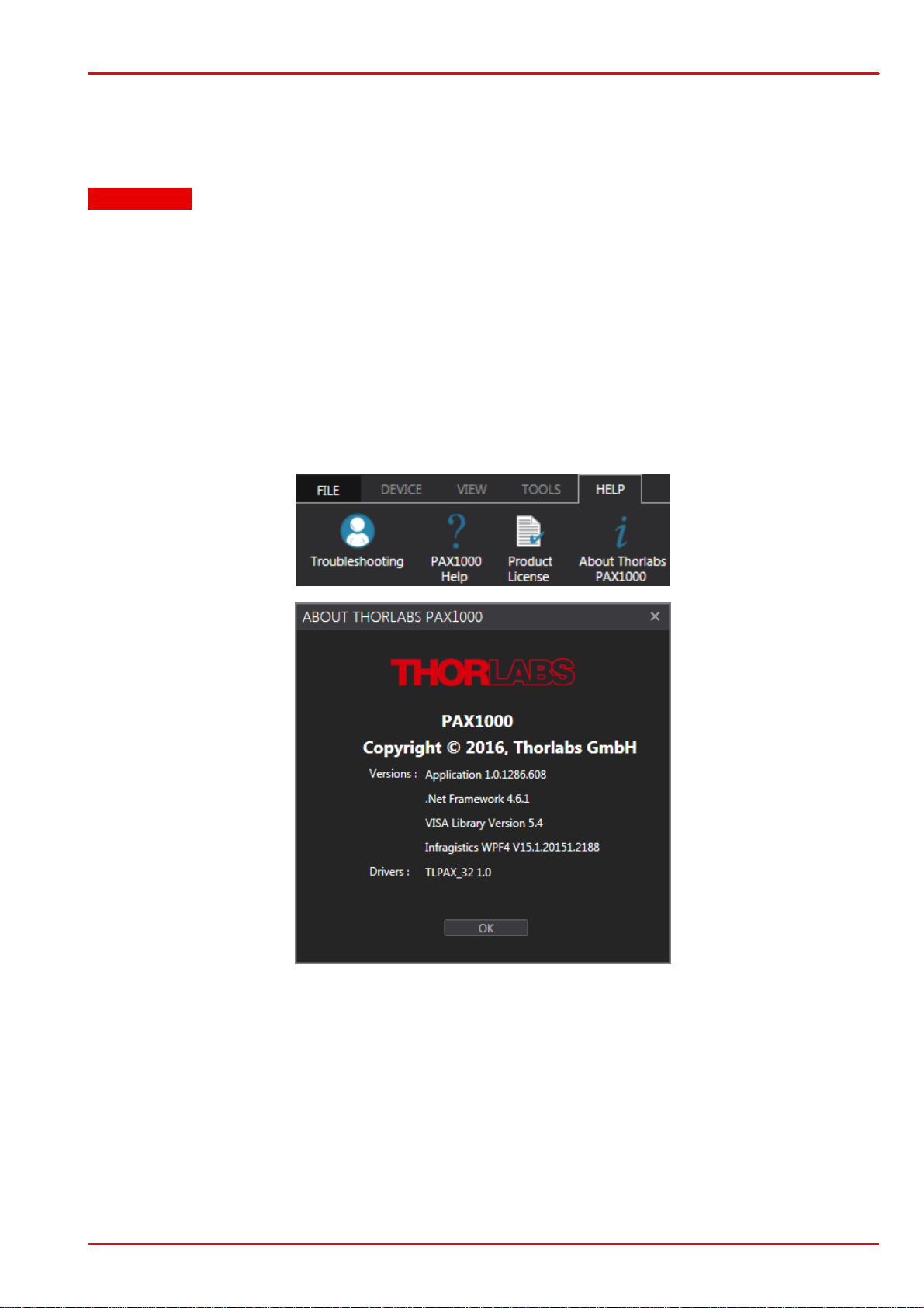
7.1 Version Information

The software version information can be found in the About dialog (ribbon HELP):

PAX1000

ADC underrun during last measurement.

ADC overflow during last measurement.

TIA gain switching is in progress.

An one-time TIA auto ranging is in progress.

An out-of-sync condition occurred during the last measurement.

Motor speed too low (too high).

PAX operating temperature is below (above) limit.

USB power supply voltage is too low.

7.2 Troubleshooting

Common Error Messages

The incident optical power was too low.

ð The PAX1000 is set to a fixed gain. ð Set the instrument to Auto Power Range or select an appropriate power range man-

ually.

The incident optical power was too high.

ð The PAX1000 is set to a fixed gain. ð Set the instrument to Auto Power Range or select an appropriate power range man-

ually.

ð This is a status message during the automatic adjustment of power range. ð No action required.

ð If this message appears, the measurement results are not reliable. The PAX1000

should resolve this error automatically.

ð If the error message persists, please contact Thorlabs.

ð This is a status message when the measurement speed was changed. ð If this message appears frequently or permanently, please contact Thorlabs.

ð This error message may appear in the case of too low (too high) environmental temper-

ature.

ð If this message appears at normal operating temperature, please contact Thorlabs.

ð The PAX1000 requires a higher operating current than the standard USB2.0 port can

deliver, e.g. at hing measurement speed.

ð Connect the external power supply.

7 Maintenance and Service

Incomplete circle due to insufficient number of measurement values. Increase fiber stress or extend measurement time.

Circle completed, but the distance between adjacent measurement points is too large for accurate measurement. Decrease fiber stress and increase measurement time.

Eigenmodes of the fiber under test are not strictly linear or measurement is noisy. ER cannot be calculated.

The circle on the Poincare sphere is too small. The calculated ER is above the theoretical maximum accuracy. Please check if stress was applied to the fiber during the measurement.

The ellipticity of some points is bigger than |25°|. Eventually there is a problem on the coupling into the fiber or there is constantly stress on the fiber.

Extinction Ratio Warnings Error Messages

The change of polarization during the measurement was insufficient to draw a full circle on the Poincaré Sphere.

ð Increase the fiber stress during measurement. ð Alternatively, increase the measurement time.

The change of polarization during the measurement was sufficient to draw a full circle on the Poincaré Sphere, but the number of measurement points was insufficient to approximate a circle with the necessary accuracy.

ð Decrease the fiber stress during measurement and increase the measurement time.

The change of polarization led to a non-circular trace on the Poincaré Sphere. ð The optical power is too low, so that noise interfered the measurement.

Check your setup for possible power loss, or increase the optical power of your laser source.

ð The fiber under test behaved not like a PM fiber.

Check if the fiber as specified as a PMF. If so, check if the operating wavelength of your PM fiber matches with the measurement wavelength.

The measured ellipticity change is close to or less than the PAX1000 measurement accuracy.

ð Was the fiber Increase the fiber stress during measurement?

The output SOP was of a too high ellipticity. ð Check your setup for proper coupling of the light source into the fiber under test. The

light must be coupled in parallel to the slow axis of the fiber.

ð Check your light source for strictly linear polarization. ð Check if your fiber under test is exposed to a permanent stress due to extreme bending

or squeezing. Also, the connectorization of the fiber might be not stress-less.

PAX1000

Linear Polarization

Elliptical Polarization

Circular Polarization

8 Tutorial

8.1 Polarization of Light

8.1.1 The Nature of Polarization

When talking about polarization, light is considered as an electromagnetic wave. It oscillates perpendicular (transverse) to the direction of the propagation of the light beam. Such a transverse electromagnetic wave can be divided into an unpolarized and polarized part. The plane of polarization of unpolarized light, also called natural light, fluctuates arbitrarily around the direction of propagation, so that in average no direction is favored.

All field components of polarized light have a fixed phase difference to each other. Each state of polarization (SOP) can be split into any two orthogonal states. The following pictures illustrate different states of polarization:

The first example is linear polarized light. The phase difference between the two orthogonal states is 0° or 180°, and superposition results in a total electric field that is always oriented in the same direction when viewed in the transverse plane.

The second diagram shows an elliptical polarization state. The phase difference between the orthogonal states is >0° and <=90°. The projection results in an ellipse with a right or left direction of rotation.

A special case of elliptical polarization is circular polarization (3rd example), where the phase difference between the orthogonal states is 90°. Then the amplitude of the rotating vector is constant over the entire 360° rotation.

Common light sources except lasers emit natural light. Helium Neon lasers or DFB laser diodes normally feature linear polarization. However, if this laser light is launched into a single mode standard fiber (SMF), the linear polarization is transformed into an arbitrary polarization.

Even if a polarization maintaining fiber is used, the linear polarization has to be coupled into one of the main axes to prevent the loss of linearity.

A multimode fiber allows a propagation of numerous modes. The state of polarization of each mode at the end of the fiber is arbitrary. The superposition of the polarization of all modes results in unpolarized light.

The spectral width of the emitted light needs to be considered as well. If the spectral line width of the emission is narrow enough, then the light is polarized. An example is a DFB laser diode with a linewidth of about 3MHz.

Light sources with a broad spectrum like LEDs are generally unpolarized. A polarizer can be used to polarize light with a large spectral width.

8 Tutorial

Right-Circularly Polarized Light

Left-Circularly Polarized Light

8.1.2 Handedness of Polarization

Convention

When light is elliptically polarized, the electric field (E field) vector rotates with respect to a Cartesian coordinate system as it propagates. The software of the PAX1000 and the predecessor, the PAX57xx Polarimeter System, plot the E field vector with respect to a right-handed coordinate system with x, y, and z axes. The light wave propagates in the +z direction, and the (virtual) observer looks along the -z direction towards the light source. The handedness of the elliptically polarized light describes the direction of rotation of the E field vector as seen by this observer. This convention is common in the technical literature.

Each state of polarization can be split into two linearly polarized orthogonal components, in which one is oriented in the x direction and one in the y direction. If both components have

equal magnitudes and the phase shift of the y component relative to the x component is +p/2 or

-p/2, the light is circularly polarized. The sign of the phase difference determines the handedness of the rotation. A clockwise rotation corresponds to a right-hand circular polarization state

and a phase shift of -p/2, while a counterclockwise rotation refers to left-hand circular polarization state and a phase shift of +p/2.

In above figures, the projection of the rotating E field vector on a virtual screen generates a circle over time as the E field vector rotates clockwise (counterclockwise) representing right (left) circular polarization.

Generation of Circularly Polarized Light

A circular polarization state can be generated using linearly polarized light and a quarter waveplate. When the E field vector of the incident linearly polarized light is oriented at a 45° angle to the slow and fast axes of the quarter waveplate, the output light is circularly polarized. It is convenient to mathematically describe this transformation using matrix algebra, with Jones vectors representing the polarized light and a Jones matrix representing the quarter waveplate. The Jones matrix, describing a quarter waveplate with its slow axis oriented along the x (horizontal) axis is:

The phase factor e

ip/4

can be omitted in almost all cases.

PAX1000 The Jones vector of a linear polarization state oriented at + 45° is written as:

When this linearly polarized light travels through a quarter waveplate, the Jones vector of the output light can be calculated as follows:

The output polarization is right-hand circular. The figure below illustrates this case:

The slow axis of the quarter waveplate are aligned with the x axis, and the fast axis of the QWP is aligned with the y axis of the coordinate system. The input polarization is +45° linear and it is transformed into a right-hand circular polarization. The purple vector at the origin indicates the orientation of the incident +45° linearly polarized light, while the red and blue vectors represent this E field decomposed into its orthogonal components. These two components are in phase. The x axis component, which is represented by the blue vector, is aligned with the slow axis of the waveplate and travels at a slower velocity through the waveplate than the y axis component, which is aligned with the fast axis and represented by the red vector. Propagating through the waveplate, the phase of the x axis component is retarded with respect to the phase of the y axis component. The amount of the retardation is determined by the thickness of the waveplate. A quarter waveplate is designed to into-

duce a phase shift of -p/2. This retardation results in a right-hand circularly polarized output light, and its E field vector rotates clockwise when it propagates along the z axis.

When the incident beam has a -45° linear polarization, its Jones vector is:

The output polarization state is then expressed:

The output light is left-hand circularly polarized.

8 Tutorial

Above illustrates this case.

Again, the slow axis of the quarter waveplate are aligned with the x axis, and the fast axis of the QWP is aligned with the y axis of the coordinate system. The input polarization is -45° linear and it is transformed into a left-hand circular polarization.

The purple vector at the origin again represents the orientation of the incident linearly polarized light. As for this, there is no phase difference between the x and y axis components of the E field. The -45° orientation of the polarization vector means that it is azimuthally rotated. Propagating through the quarter waveplate causes the component aligned along the slow axis

to add a phase shift of +p/2 with respect to the component aligned along the fast axis. The output light is left-hand circularly polarized and has an E field vector that rotates counterclockwise when it propagates along the z axis.

PAX1000

State of Polarization

Jones Vector

Horizontal Linear Polarization

Vertical Linear Polarization

Linear Polarization at +45°

Linear Polarization at -45°

Right Circular Polarization

Left Circular Polarization

Linear optical Element

Jones Matrix

Horizontal Linear Polarizer

Vertical Linear Polarizer

Linear Polarizer at +45°

Linear Polarizer at -45°

Quarter Wave Plate, Slow Axis Horizontal

Quarter Wave Plate, Slow Axis Vertical

Jones Vectors and Matrices

The following tables contain the Jones vectors for selected polarizations of light and the Jones matrices of standard optical elements, respectively.

8.1.3 Mathematical Representation of an Electromagnetic Wave

An electromagnetic wave of frequency w traveling in Z direction has its polarization vector in the X-Y plane. The E-field direction is always perpendicular to the direction of propagation. Any loc- ation of the polarization vector at different times t can be written by superposition of the X- and Y- vector components:

with:

ÊX, Ê EX, E

δX, δY Phase of the electric field intensity in X or Y direction, -p

Amplitudes of the electric field intensity in X or Y direction

Instantaneous electrical field intensity in X or Y direction

, δY p

w Angular frequency k Wavenumber

The wavenumber k can be calculated by the frequency or wavelength:

with:

n Refraction index c Speed of light

l Wavelength in vacuum

Jones Vector Formalism

In optics, polarized light can be described using the Jones calculus, developed by R. C. Jones in 1941 [1] . Polarized light is represented by a Jones vector, and linear optical elements are

represented by Jones matrices. The Jones vector describes the polarization of light in free space or another homogeneous isotropic non-attenuating medium, where the light can be prop-

erly described as transverse waves. Omitting the time dependency e

jwt

, the electromagnetic

wave can be fully characterized by the complex envelopes:

of the X and Y components of the electric field. The Jones vector is then

The Jones vector is not a vector in real space, but a mathematical abstraction in complex space. The following figure shows the spatial curves of the X and Y components of the electric field intensities as a function of time:

PAX1000

Origin of a Circular Polarized Wave

The vector of the electric field intensity E(t) is determined by the superposition of the X and Y components. At a fixed time it points to a defined direction and has a defined magnitude.

The following figure is used to illustrate a case of circular polarization, in which Êx=Êy, dx=180° and dy=90°.

When these values and the times noted beneath each of the following figures are inserted into equation [1] , Ex and Ey values for each case can be calculated.

The vector sum of Ex and Ey is the total electric field intensity E. In this example, the head of the vector moves anti-clockwise around the circumference of a circle as the wave propagates

toward the observer. When Êx¹Êy, the electric field vector traces out an ellipse.

When the phase difference between the Ex and Ey components is 0°, instead of 90°, the circle becomes a line, which corresponds to linearly polarized light.

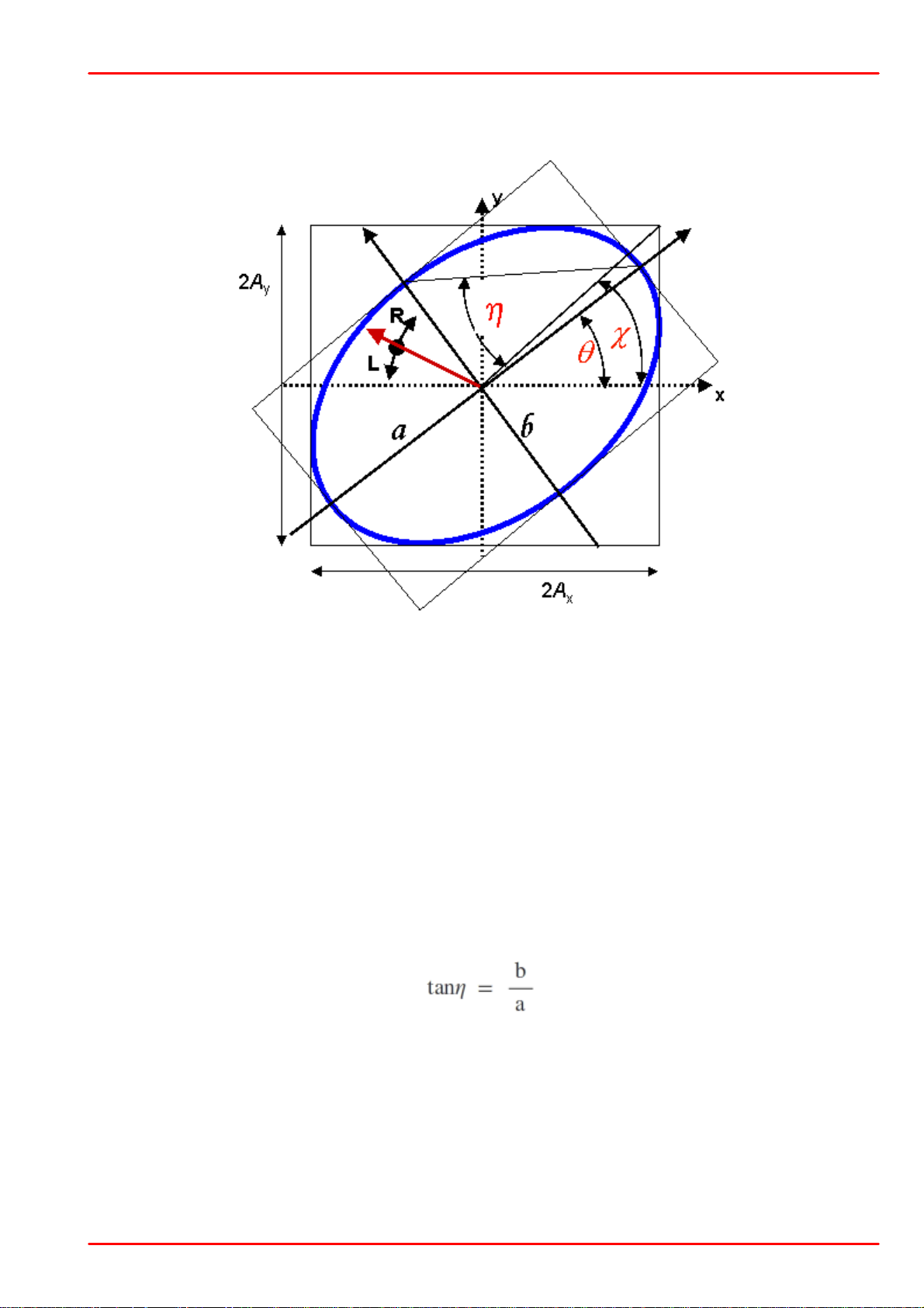
8.1.4 Polarization Ellipse

The state of polarization can be represented by an ellipse:

8 Tutorial

The (virtual) spectator looks towards the light source. Definition of right and left handed polarization: The right hand rule is used to describe the handedness of the polarization state. The right hand

rule is used in a Cartesian coordinate system with X, Y, and Z axes, and the name of the rule comes from the ability to use the right hand to apply the rule. The handedness of the polarization state can be determined from propagation direction, or vice versa. When determining the handedness of the polarization state, point the thumb of the right hand along the direction of light propagation. The fingers curl in the direction of the rotation of right hand polarized light around the ellipse. Left hand polarized light propagates in the opposite direction.

The parameters ellipticity (h) and azimuth (q) as well as the handedness (right and left which corresponds to the sign of h) are necessary to uniquely describe the polarization. The azimuth angle q is the angular deviation of the major axis of the ellipse from the X axis. The angle h is

calculated from the ratio of the semi-minor (b) to the semi-major (a) axis dimensions according to the following equation:

h > 0: The light is right-handed polarized. h = 0: The light is linear polarized. h < 0: The light is left-handed polarized.

An ellipse can also be described by the parameters angle c and phase j. The handedness is defined by the sign of j.

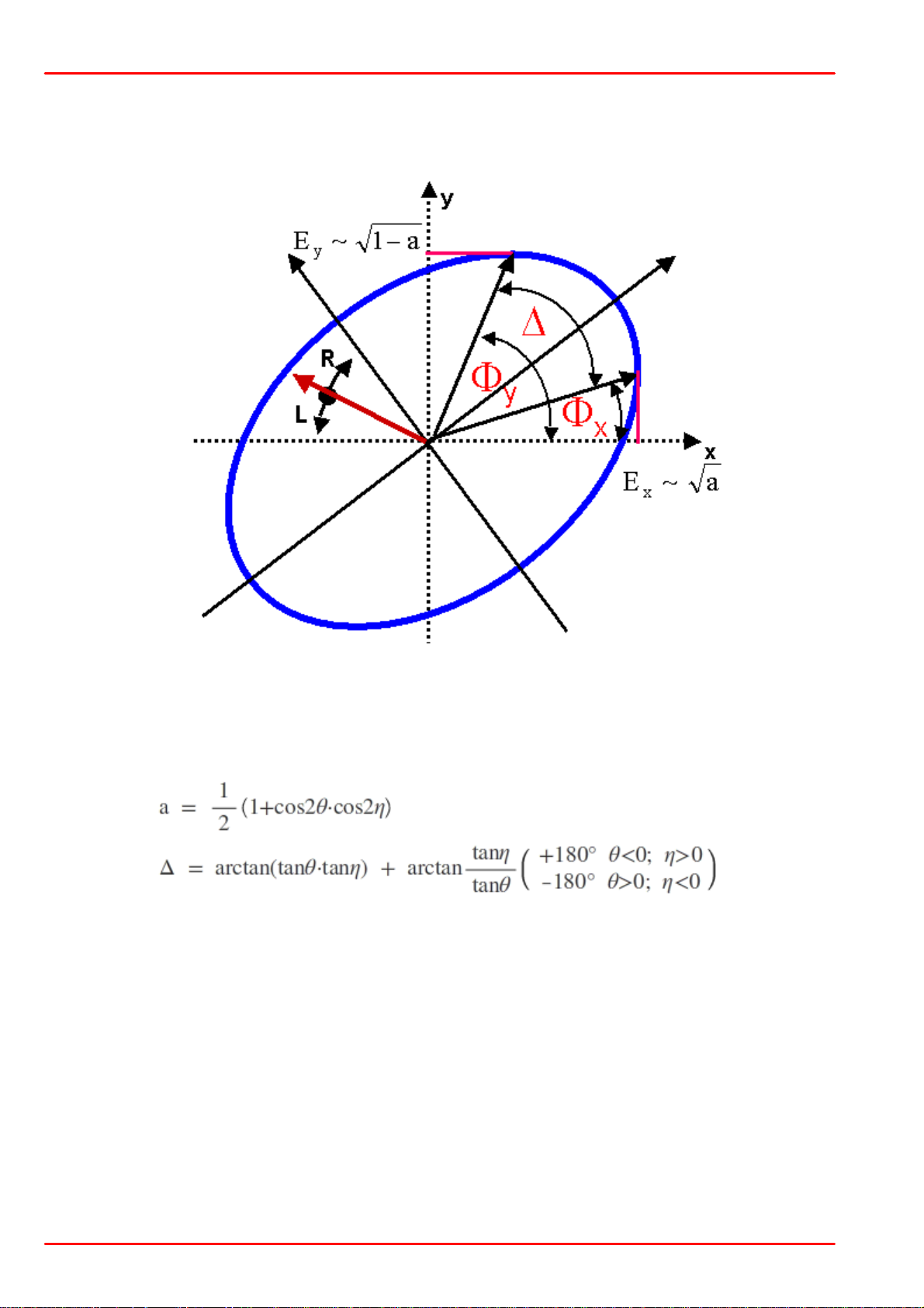
PAX1000

Another way to determine an ellipse is to use the power split ratio a and the phase difference D. The power split ratio is defined between 0 £ a £ 1 and the phase difference can obtain values between -180° £ D £ 180°.

The power split ratio and the phase difference can be calculated from azimuth and ellipticity by the following formulas:

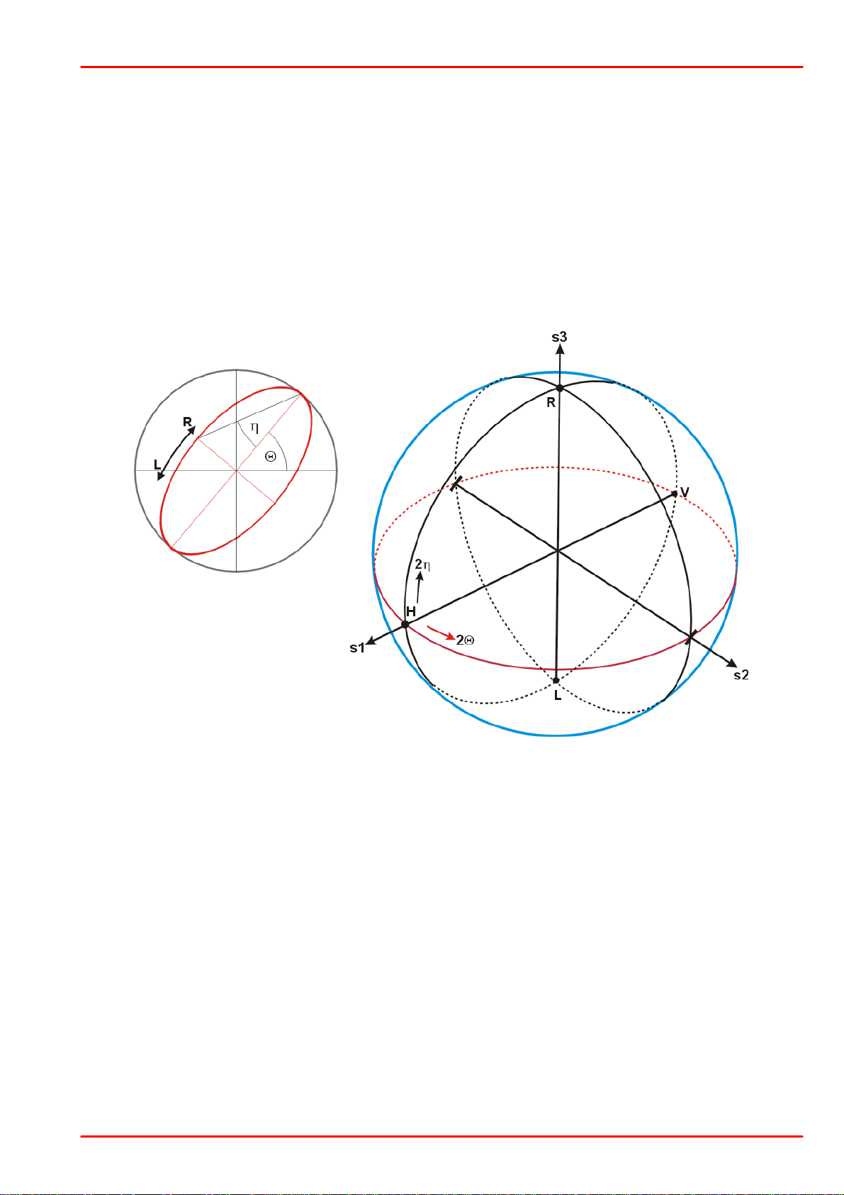
8 Tutorial

Polarization State

Azimuth q

Ellipticity h

H linear, horizontal

0°

/ linear +45°

45°

0°

V linear, vertical

±90°

0°

\ linear -45°

-45°

0°

R right circular

+45°

L left circular

-45°

8.1.5 Poincaré Sphere

An appropriate way to display the state of polarization is the Poincaré sphere representation. The center of the Poincaré sphere is located in the origin of a Cartesian coordinate system.

Any point on the surface of the Poincaré sphere is uniquely represented by its Cartesian coordinates, also known as the 3 normalized Stokes Parameters s1, s2 and s3 - these are the projections of this point onto the three coordinate axes.

The polarization ellipse parameter azimuth (Θ) angle is represented on the Poincare sphere as the longitude = 2Θ, the ellipticity (h) angle appears as the latitude = 2h. Please note the factor

of 2 involved in the mapping - the figure below illustrates that. The handedness defines the position on the northern (right handed rotation) or southern (left handed rotation) hemisphere.

The equatorial plane (shown in red) represents all linear states of polarization. The north pole represents right-turning circular polarization, the south pole - left-turning circular polarization. All other points on the northern and southern hemisphere correspond to elliptical states of polarization with correspondingly right and left handed rotation. Below are given some typical states of polarization, and their azimuth and ellipticity values:

Changes of the state of polarization as a function of time can be displayed as a trace on the Poincaré sphere.

PAX1000

Bow-Tie fiber

PANDA fiber

8.1.6 Polarization in Fibers

Different types of optical fiber affect the polarization state of the propagating light differently. The most common types of optical fibers are multimode, single mode, and polarization maintaining.

There are many different types of multimode fibers (MMFs), but all support more than one guided optical mode. In most cases, MMFs support hundreds or thousands of optical modes. The exact modes excited by the input light, and the power distribution among them, depend on input coupling conditions. Each mode travels at a different velocity, and mode mixing occurs at bends and other points of inhomogeneity within the fiber. The SOP of light that has propagated through a MMF is totally arbitrary, which makes MMFs incompatible for use with applications that require preserving polarization states.

Single mode fibers (SMFs) support only one guided mode, but this mode consists of two components with orthogonal polarizations. An ideal fiber has a perfectly cylindrical geometry, as well as an index of refraction profile that is radially symmetric and unchanging down the length of the fiber. The orthogonal polarization components in an ideal SMF propagate at the same velocity, as well as independently of one another without mixing. Under these perfect conditions, the input and output SOPs are identical.

In actuality, an optical fiber cannot be fabricated with a perfectly cylindrical geometry. The small geometrical deviations combined with mechanical stresses, such as those occurring at fiber bends, cause the effective refractive index of the two orthogonal components to differ by a small amount (i.e. SMF exhibits low levels of birefringence). Under these conditions, the two orthogonal polarization mode components travel at slightly different velocities as they propagate down the fiber. As this delays one polarization component with respect to the other, propagating through the SMF transforms the input SOP to an arbitrary output SOP. The effect on polarization is more pronounced for longer transmission distances.

In addition, microscopic inhomogeneities in the refractive index that occur naturally during fiber fabrication, as well as microbends, can scatter (couple) light from one polarization component into the other polarization component. The similarity of the effective refractive indices of the two polarization components facilitates this scatter-induced mixing, which acts to further randomize the output SOP.

If it is of interest to preserve the polarization state of light as it propagates through an optical fiber, one approach is to design a single mode fiber that decouples the two orthogonal polarization components and keeps them from mixing with one another. Such a fiber would be designed so that the effective refractive index for light polarized in one direction differs significantly from that for light polarized in the orthogonal direction. These types of fibers, which are designed to have significant levels of birefringence, are called polarization maintaining fibers (PMF). They typically use mechanical stress or anisotropic geometries to create the difference in refractive index. In any PMF fiber, light polarized along one axis of the fiber, the “slow” axis, travels at a lower velocity than light polarized along the orthogonal, “fast” axis. An example of a PMF is one with elliptically shaped core, instead of the circularly shaped cores in SMF. Examples of stress-birefringent PMF fibers are PANDA and Bow-Tie.

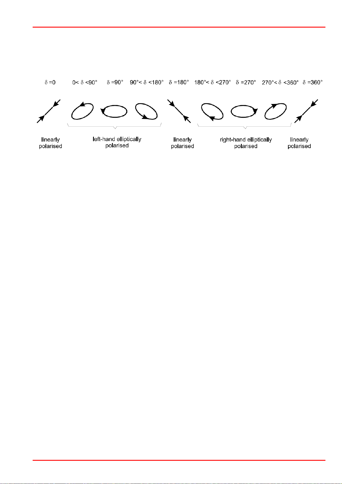
8 Tutorial

If linearly polarized light is launched into a PMF fiber such that light is coupled into both the fast and slow axes, propagation through the PMF will delay one polarization component with respect to the other. The delay creates a phase difference, d, between them. The magnitude of the phase difference, and the proportion of light carried by each fiber polarization component, determines whether the output SOP is linear, elliptical, or circular.

Due to the cyclical relationship between the phase difference and the polarization state, the two polarization states will evolve to be periodically in and out of phase as the light propagates down the fiber. The polarization components are in phase with the same direction of linear polarization when d=0° and 360°. The shortest length of fiber that results in a change in phase of

360° is called the polarization beat length. When the wavelength of the light is l, and the difference in refractive indices is dn, the polarization beat length is:

L = l / dn

If the light has propagated one beat length through the fiber, the light polarized along the slow axis lags the light in the fast axis by a distance equal to the wavelength of the light in the fiber.

While polarization beating is more easily identified in PMF, it also occurs in SMF. However, as SMF has low and variable levels of birefringence, the beat length also varies along the length of the fiber.

To ensure a linear polarization state coupled into the PMF is preserved at the output, the launch conditions must be carefully controlled. It is essential that either the fast or slow axis of the PMF is aligned with the polarization direction of the input light. Stated another way, the azimuthal orientation of the light signal must be aligned to either the slow or fast axis of the PMF. If this is not done, light will be coupled into both the slow and fast axes of the fiber and the large difference in refractive index between them will induce a short beat length of a few millimeters. The result will be frequent changes in the state of polarization along the length of the fiber, instead of the desired maintenance of the polarization state.

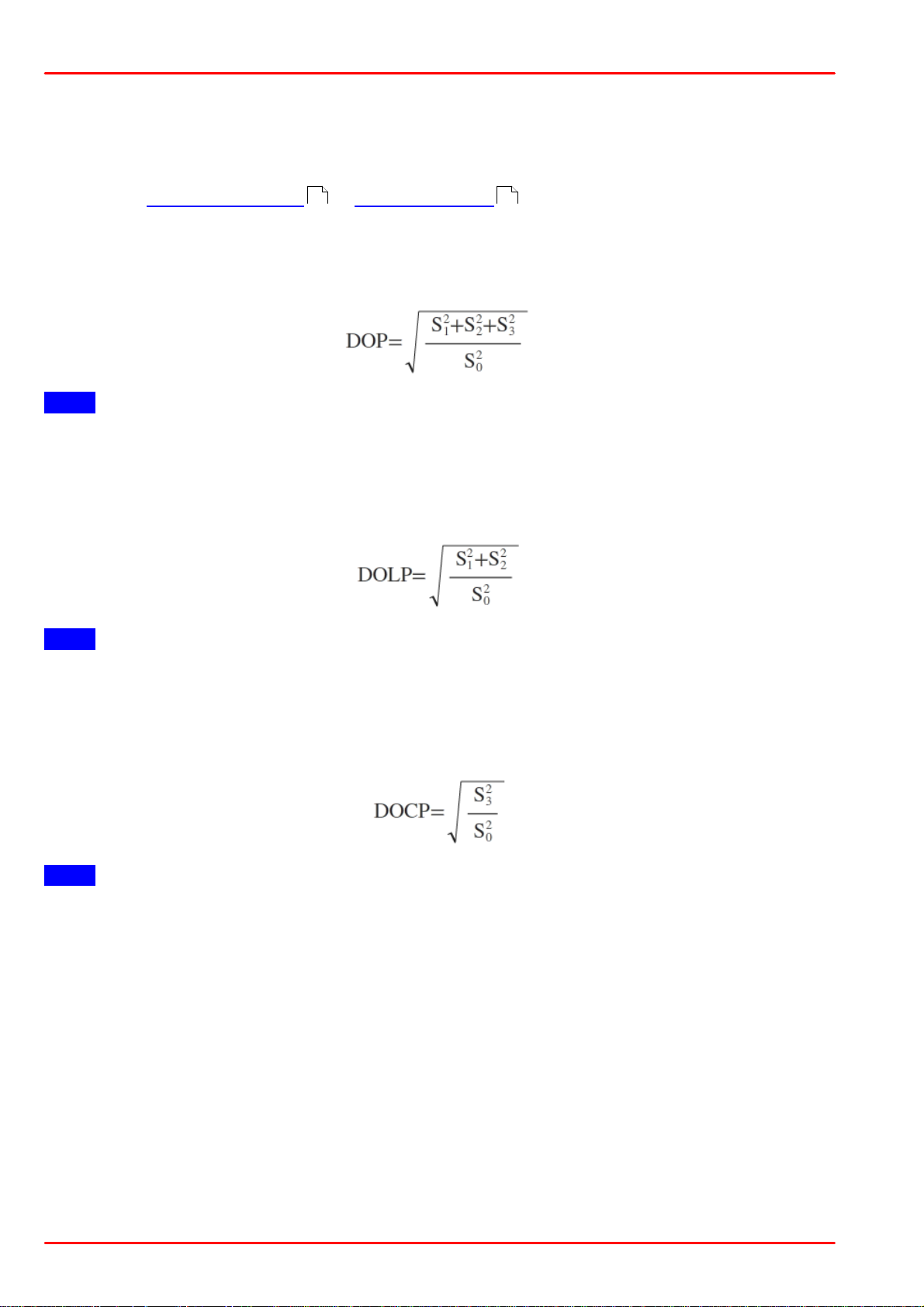
PAX1000

8.1.7 Polarization Parameters - Definitions

In this section all used in the PAX1000 software polarization parameters are explained.

Azimuth / Ellipticity

See section Polarization Ellipse or Poincaré Sphere .

60 62

DOP

Degree of polarization; it is the ratio of the polarized power to the total power of the measured light signal. It is calculated as follows,

Note

S1, S2, S3 and S0 are the non-normalized Stokes Vectors!

DOLP

Degree of linear polarization, it is the ratio of the linearly polarized share of polarized power to the total power. Its calculated as follows,

Note

S1, S2 and S0 are the non-normalized Stokes Vectors!

DOCP

Degree of circular polarization, it is the ratio of the circularly polarized share of polarized power to the total power. Its calculated as follows,

Note

S3 and S0 are the non-normalized Stokes Vectors!

Power

is the total optical power, incident on the PAX1000.

Pol

is the polarized share of the total optical power.

Unpol

is the unpolarized share of the total optical power.

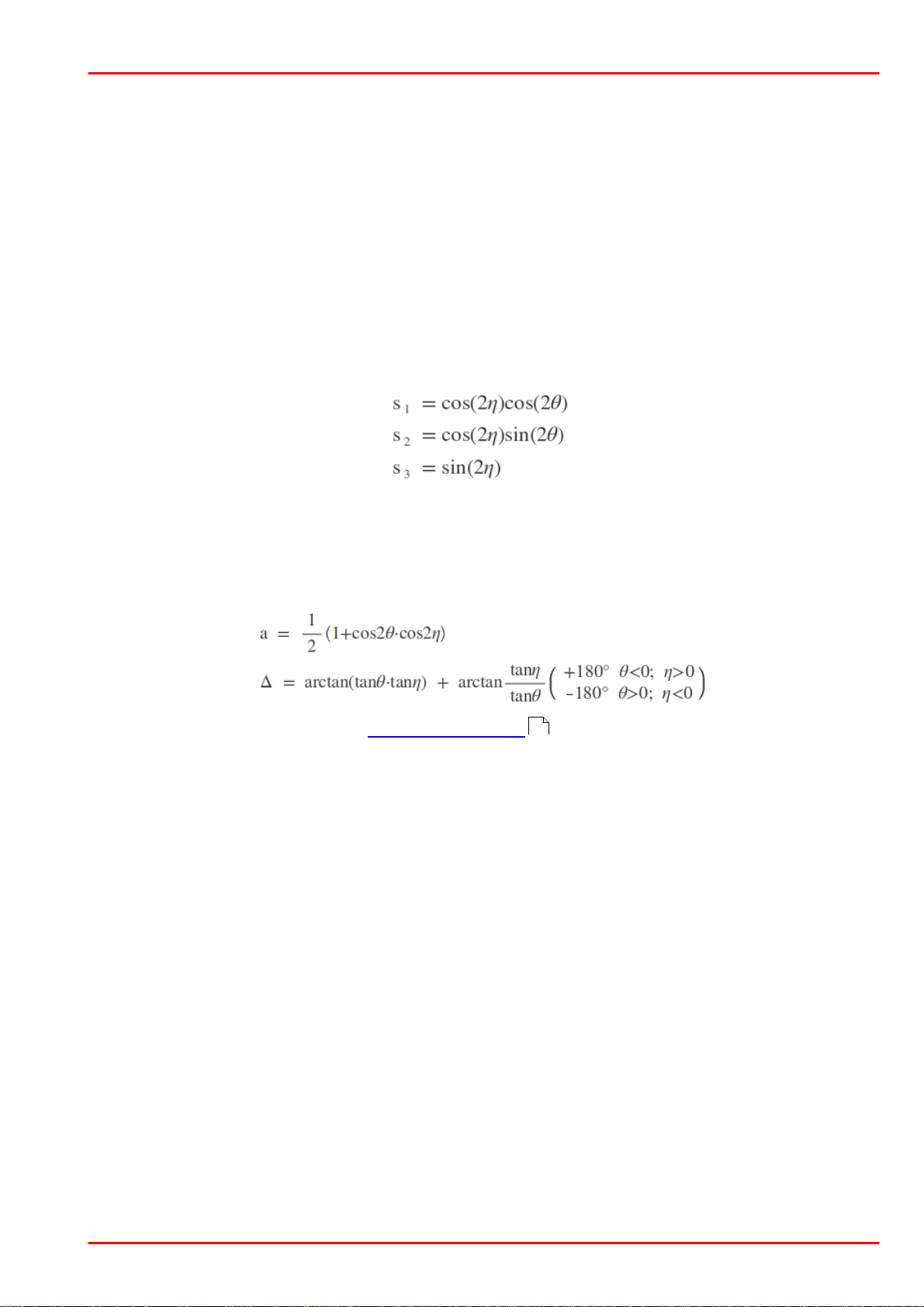
8 Tutorial

S1, S2, S3 and S0

are the non-normalized Stokes vectors. The Stokes vector represents the state of polarization (SOP) and is a four element vector (S0, S1, S2, S3), where:

· S0 is the total power

· S1 is a measure of vertical and horizontal linear polarization,

· S2 is a measure of linear polarization at 45° and –45°, and

· S3 is a measure of left and right circular polarization.

s1, s2 and s3

These are the Stokes vectors that are normalized with the total power S0 as reference. There is the following relation between the azimuth θ and ellipticity h and the normalized Stokes para-

meters:

Power Split Ratio and Phase Difference

These parameters can be alternatively used to represent the polarization state based on an ellipse. This representation has the advantage that the retardation of the Ex vector to the Ey vec-

tor is simply defined by the phase difference ∆ :

For more information, please see Polarization Ellipse section.

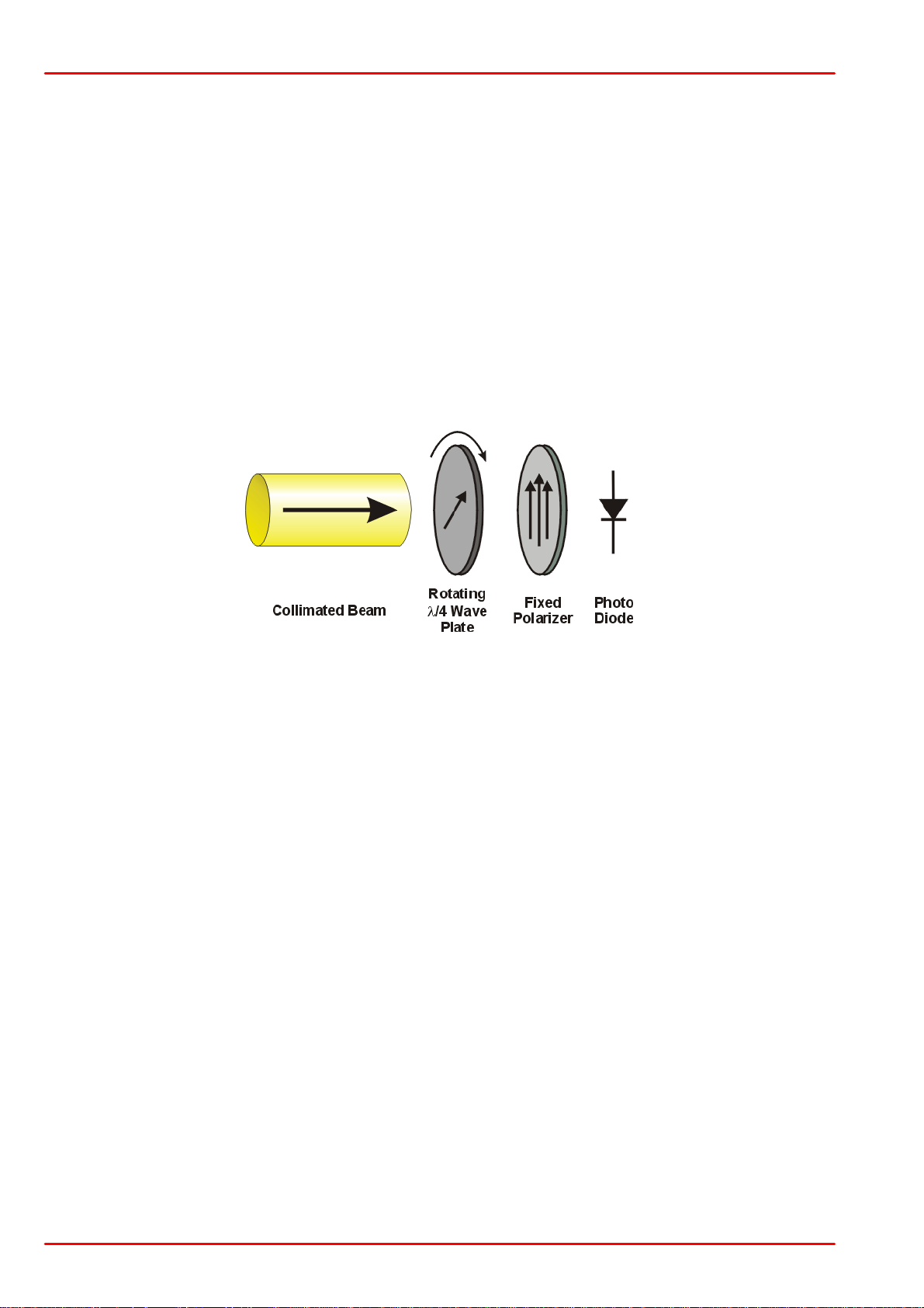
PAX1000

8.2 Polarization Measurement Technique

There are different methods to measure the state of polarization. Among them, the four detector method is a well known technique. A similar technique can be used to measure the polarization in fibers. Pairs of special Fiber Bragg grating (FBG) couple out a portion of light. The polarization can be calculated from the power ratios.

Different methods are used to measure the polarization state. Among them, the rotating l/4 waveplate technique is well known. It is described in the following section.

8.2.1 Rotating Waveplate Technique

The optical unit of the PAX1000 polarization measurement sensor consists of a rotating true zero order quarter waveplate (QWP), a fixed linear polarizer and a photodiode. The waveplate transforms the input polarization. The polarizer transmits only the portion of light that is orientated in parallel to its transmission axis. The photodiode acts as a power meter.

The incident polarization is transformed (modulated) by the rotating QWP and the polarization state that enters the linear polarizer depends on the actual rotation angle of the waveplate.

The linear polarizer transforms the polarization modulation into an amplitude modulation of the light power that enters the photodiode.

The photodiode delivers a current proportional to the optical power and to the square of the electric field intensity. It is easy to see that unpolarized light will generate a constant optical power at the input of the photodiode, as it has no defined polarization state. In general, there are only three spectral components in the photo current:

· a DC component, arising from the unpolarized optical power,

· a component with double the rotation frequency of the QWP and

· a phase-shifted component with quadruple the rotation frequency of the QWP.

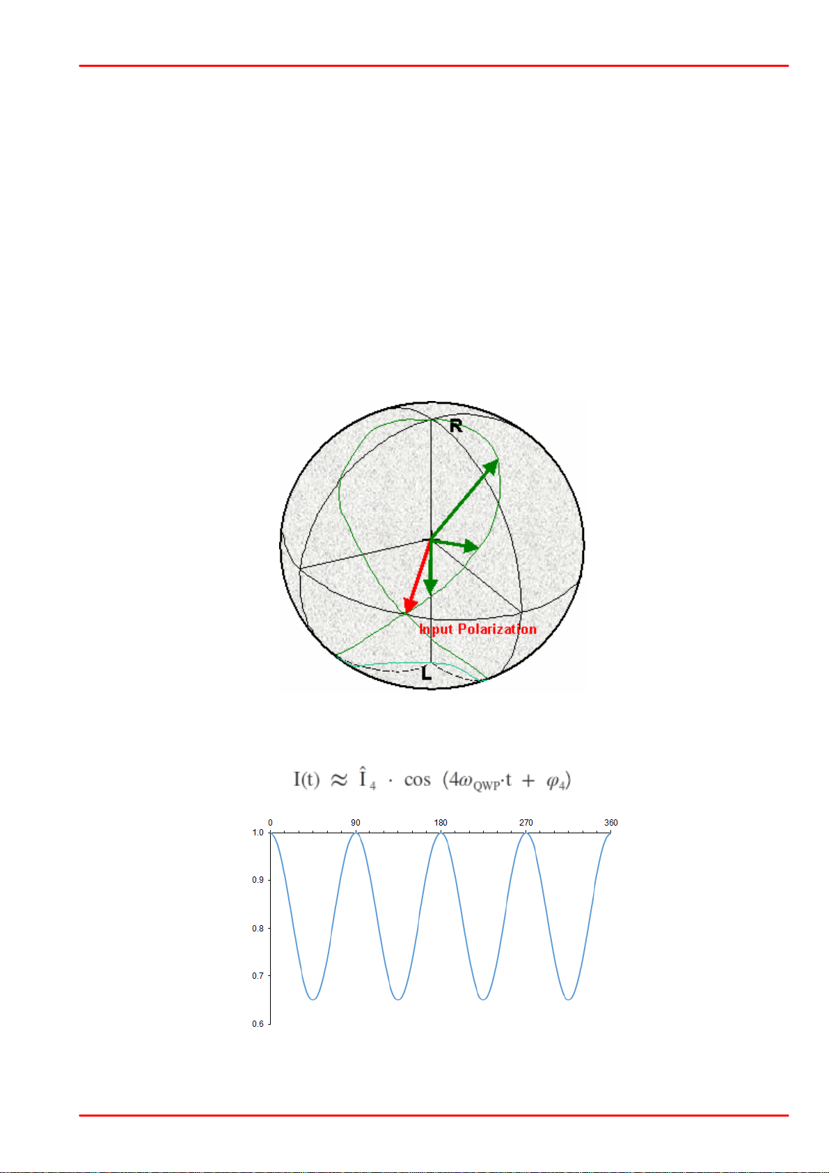
8 Tutorial

Linear Polarization

This section considers input light with a linear state of polarization (SOP). Assume that for a rotation angle of 0° the fast axis of the quarter waveplate is aligned with the polarization direction of the input light. The linear polarized light travels along the fast axis and is not changed. When the waveplate is rotated 45°, the SOP is transformed to right circular. Another 45° rotation, which gives in total 90°, aligns the slow axis of the waveplate with polarization direction of the incoming light. The SOP is not changed by the waveplate. A rotation of 135° yields left circular polarization.

A half turn, corresponding to 180°, again aligns the fast axis of the waveplate with the polarization of the light. The waveplate does not change the SOP.

The following picture demonstrates the change of the polarization on the Poincaré Sphere. The dark-green trace represents points laying in the foreground of the sphere, the light-green - in the background ("dark side"). As can be seen, after a half revolution of the QWP, a trace with the shape of an "8" is drawn onto the sphere:

In the case of linearly polarized incident light, the photo diode current I(t) is proportional to the quadruple rotation frequency, w

, while the phase shift, j4, reflects the azimuth angle:

QWP

PAX1000

Circular Polarization

This section considers the case of right circularly polarized light incident on the QWP . Circular polarization will be transformed into linear polarization by a quarter waveplate. Rotating the waveplate rotates the azimuth angle of the generated linear polarization. When plotted on the Poincaré sphere, the polarization state moves around the equator as the QWP rotates. A full revolution of the waveplate results in two turns around the equator (green trace on the figure below):

After passing the linear polarizer, the frequency of the resulting amplitude modulation is proportional to twice the rotation frequency of the QWP, and the phase of this component is constant and in this example zero:

8 Tutorial

General case

Linear and circular polarizations are special cases of polarization. Elliptical polarization generates a photodiode current with a DC term, a term that varies with twice the rotation frequency of the waveplate, and a term that varies with four times the rotation frequency of the QWP.

The Fourier transformation of the resulting photodiode current obtains the amplitudes and phases of the DC, the 2w and the 4w QWP components.

The DC component has an amplitudes of A0, the 2w component has an amplitude of A2 and a phase of j2, and the 4w QWP component has an amplitude of A4 and a phase of j4. Other fre-

quency components are assumed to have zero amplitude, in accordance with theory.

The polarization parameters azimuth, ellipticity, degree of polarization (DOP) and the Stokes parameters can be calculated from the amplitudes A0, A

and A4 and the phases j2 and j

, ac-

cordingly.

A typical photo current for elliptical polarization for one waveplate revolution is displayed in the following figure:

Note

In the PAX1000 a true zero order l/4 waveplate is used. For this type of waveplate, the exact l/4 retardation is given only at its reference wavelength. In order to enable a broad operating

wavelength range of the polarimeter, the wavelength-dependent retardation must be compensated in order to achieve accurate measurements. For this reason, the operating wavelength must be entered into the device settings.

PAX1000

8.3 Polarization Control and Transformation

The polarization of light can be manipulated by retarders, polarizers and other polarization optics. Even single mode fibers operate on the polarization state of the guided mode, so that the input and output states of polarization differ. Polarization control is important since many optical components require a well defined polarization state. In many applications, a polarization controller is a key component. In the following sections a short summary of polarization controllers is given.

8.3.1 Bulk Optics

Polarizers transmit only those light waves with a specific polarization, which makes them useful as optical filters when analyzing the light's SOP. Linear polarizers pass one of the two orthogonal components of light. They generate linearly polarized light aligned with the transmission axis of the polarizer. Circular polarizers can have a clockwise or counterclockwise orientation, and they pass clockwise or counterclockwise generated light, respectively. If two polarizers are used in an optical setup, the second is called an analyzer.

Retardation Plates (Retarders) can be used to control the polarization of a light wave. In general, a retarder is a birefringent optical element, in which orthogonally polarized components of light have different indices of refraction. Light incident on a waveplate is divided into one component polarized along the fast axis, which has a lower index of refraction, and one polarized along the slow axis, which has a higher index of refraction. Traveling through the waveplate delays the light polarized along the slow axis relative to the light polarized along the fast axis, so that a there is phase difference between them. After passing through a QWP, the slow axis

lags the fast axis by l/4 and the phase difference is 90°. Quarter waveplates convert elliptically polarized light to linearly polarized light, and vice versa. After passing through a half waveplate,

the slow axis lags the fast axis by l/2 and the phase difference is 180°. A half waveplate flips the polarization direction of linear light with respect to the fast axis and inverts the handedness of elliptically polarized light.

Polarization Controller consisting of one half waveplate placed between a pair of quarter waveplates can be used to produce light with any SOP from arbitrarily polarized input light.

The first QWP is adjusted so that linearly polarized light is incident on the half waveplate. The half waveplate is rotated to adjust the azimuth angle of the light incident on the second QWP. The second QWP transforms the incident linearly polarized light into elliptically polarized light. For QWPs and half waveplates, if the incident light is linearly polarized and its direction of polarization is aligned to the fast or slow axis, the light passes unmodified through the optical element. If a QWP is aligned so that the azimuth of the input light is at 45° to the fast and slow axes, a circular state of polarization is generated.

8.3.2 Fiber Polarization Controllers

A fiber optic polarization controller (aka Lefèvre loops) is used to accurately set the state of polarization of light in a single mode fiber. These polarization controllers apply bend-induced

mechanical stress to the fiber to induce birefringence, so that the orthogonally polarized components of the guided fundamental mode travel at different velocities. By controlling the length of fiber over which the stress-induced birefringence is applied, the function of bulk QWPs and half waveplates, which are described in the Bulk Optics section, can be duplicated in optical fiber. As the stress-induced birefringence in the fiber is low compared with the birefringence of the bulk optic crystals, relatively long lengths of fiber (typically on the order of 1 m) are needed to induce the desired phase shift. The mechanical stress is induced by wrapping the fiber around a spool, and the number of turns determines the total phase shift induced between the two polarization components.

8 Tutorial

A fiber polarization controller features two l/4-paddles and one l/2-paddle. These three paddles can be twisted relative to one another. The diameters of the paddles are chosen in such a way that all states of polarization can be set. Therefore, 1/2/1 or 2/4/2 turns are necessary, depending on the wavelength range. A rotation of a paddle causes a rotation of the fast and slow axes in the fiber spool with respect to the incoming electric field.

Another way to cause birefringence in a SMF is to "squeeze" the fiber. Applying pressure to the fiber results in stress birefringence. By setting up three independent fiber squeezers in series with a 45° shift each to the other, any desired transformation of polarization can be achieved. The disadvantage of a fiber squeezer is the strong mechanical stress imposed upon the fiber that may lead to destruction.

8.3.3 Fiber Polarization Scrambler

Polarization scramblers convert highly polarized light into light with a random polarization. Piezoelectric components, also known as fiber squeezers, are used to quickly modulate the state of polarization by inducing a time-dependent birefringence in the optical fiber. Thus it is

possible to reduce polarization dependent effects in optical transmission systems, for example, polarization dependent losses or gain. Polarization scramblers should have a low insertion loss and operate in a wide wavelength range.

PAX1000

8.4 Extinction Ratio Measurement on PM Fibers

8.4.1 Definition

A Polarization Maintaining Fiber (PMF) is only effective if linearly polarized light is launched parallel to the fast or slow axis. The ratio of the power in the fast and slow axis (in dB), the so-called Extinction Ratio (ER), is a measure of the quality of this coupling.

The extinction ratio is measured at the output of the PMF. First the polarization state is described using the polarization ellipse, which is the 2D curve traced out by the rotating polarization vector. The length of the major and minor axes of the ellipse are proportional to the amount of optical power coupled into the two axes of the PMF. For example, if all power is coupled into one axis, the ellipse will be a line, and if the power is evenly split between the two axes the ellipse will be a circle. As the instantaneous position of the polarization vector on the ellipse is a function of the distance from the output of the PMF, the measurement plane should be translated back and forth to determine the maximum and minimum values of optical power, P

and P

MainAxis2

, respectively.

MainAxis1

Given a linear polarization state launched optimally into either the fast or slow axis, the ER expresses the ability of the PMF to maintain that state by suppressing cross-coupling that would transfer power to the orthogonal polarization state. The ER is therefor a crosstalk specification. If the ER is poor then either the PMF has a poor polarization preserving capability (or enhanced mode coupling) or the alignment into the PMF is not optimal.

A PMF preserves the linear polarization state of the input only if the polarization state at the input is linearly polarized and perfectly aligned with one of the principal PM axes (polarization eigenstates).

If linearly polarized light is coupled into both the fast and the slow axes of the PMF, the two components will propagate independently of one another through the fiber. For this discussion it can be assumed that there is no cross-coupling between them. Due to the PMF's birefringence, the phase shift between the two components increases continuously with propagation distance through the fiber. Consequently, the polarization ellipse also depends on propagation distance. The accumulated phase shift at the fiber exit point depends on the wavelength of the light source, the length of the PMF, and the fiber birefringence. The polarization ellipse will be affected by a change in any of these parameters. This phenomenon is the reason it is critical to optimally align linearly polarized optical input with one axis of the PMF, whether the optical input is from a laser or from another PMF.

8.4.2 Measurement

For ER measurement the fiber must be dynamically "stressed" during data acquisition by

· either mechanically "pulling" the fiber

· or heating or cooling the fiber

· or changing the wavelength.

There are two different main techniques for Extinction Ratio (ER) Measurement of PM fibers. One is based on a polarimeter while the other utilizes a rotating analyzer (polarizer) and a photodiode based power meter.

The two techniques cannot be compared directly since the polarimeter technique does not take into account the depolarized part of the light and is focused only on the relative change of the polarization and not on the absolute ellipticity.

8 Tutorial

An ER meter based on the rotating analyzer considers the Degree of Polarization (DOP) as well as the absolute ellipticity.

Polarimeter Technique

The polarimeter records the polarization at the exit of the fiber during stress application. If there is a non-optimal launch condition (misalignment) or a poor fiber, the output polarization will result in a circle being traced on the Poincaré sphere, in which the diameter of the circle is a measure for the extinction ratio. The smaller the circle the higher is the ER:

ER Meter Technique

Thorlabs' ERM100 is based on a rotating polarizer.

The polarizer transmits only the polarized part of the light parallel to its transmission axis. The transmitted power depends not only on the input polarization but also on the degree of polarization (DOP). A photodiode after the spinning polarizer detects the power.

If the input light is linearly polarized and the DOP is 100%, the measured photo current is sinusoidal with its minimum at zero.

An elliptical input polarization or a DOP less than 100% causes a minimum > 0 of the photodiode current. However, there are more factors that can influence the measurement data like dark current and noise of the photodiode, but these are neglected for our considerations.

If the input light is circularly polarized with a DOP of 100% a constant (DC) photocurrent would be the result. A purely unpolarized input light would also generate a DC photo current.

Both the ellipticity as well as the DOP will affect the measurement result. This should be considered when measurements with the ERM100 are performed.

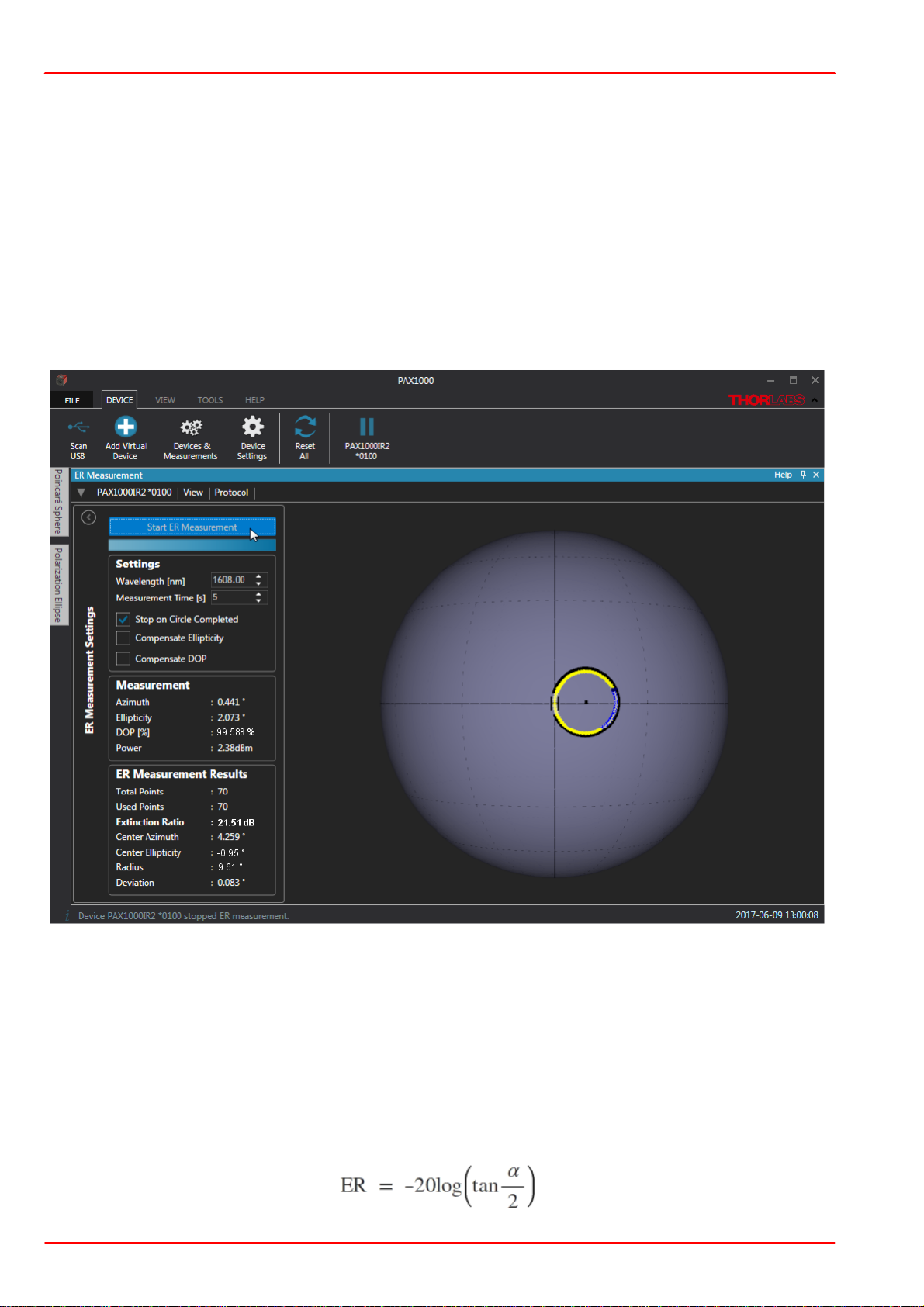
PAX1000

ER Measurement Screen of a Thorlabs PAX1000

8.4.3 Correction of the Polarimeter ER Measurements

When performing ER measurements on PM fibers with a polarimeter, the DOP will not affect the measurement results and only the relative polarization changes (circle on the Poincaré Sphere) are taken into account.

Correction for absolute ellipticity

Ideally, optimally coupling linearly polarized light into either the slow or fast axis of the PM fiber ensures that linearly polarized light will be output from the fiber. However, externally applied mechanical stress, such as from fiber connectors, can cause the propagating light to undesirably couple into the orthogonal polarization. This cross-coupling will transform the linearly polarized light into elliptically polarized light. A polarimeter measurement can determine the ER of the output light, as shown in the figure below.

The center of the circle represents the center Azimuth and Ellipticity. It should be positioned on the equator. As the light is predominantly linearly polarized, the center of the circle should be positioned on the equator. Each measurement point can be expressed as an Azimuth / Ellipticity pair. Plotting all measurement points will describe a circle. The measurement value which is most distant from the equator has the maximum ellipticity.

In above example, the measurement of the ER was 21.51dB. This measurement is based only on the relative polarization changes (circle on the Poincaré Sphere) during the measurement. The radius is 9.61°. The formula to calculate the ER is as follows:

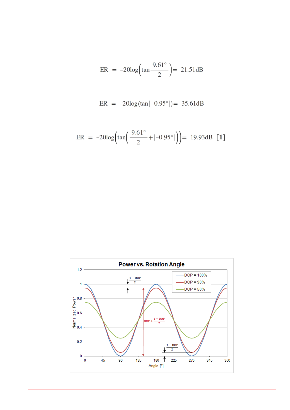
8 Tutorial

Impact of the DOP on the ER Result (Spinning Analyzer Method)

α is the radius in degrees. The factor ½ is due to the fact that azimuth and ellipticity are

mapped with a factor ½. The domain for azimuth is -90° to 90° (180° area). A circle has a range of 360°.

In our measurement example this yields:

The center ellipticity is -0.95°. That means even if the circle would have a radius = 0, an ellipticity remains. This center ellipticity corresponds to

Both the radius and the center ellipticity have to be considered. The maximum ellipticity corres-

ponds to α/2 + | center ellipticity |:

This is the corrected for center ellipticity ER.

Correction for DOP (Degree of Polarization)

A polarimeter's ER measurement must also be corrected for DOP, as the unpolarized part of the light is not considered. In other words, while the DOP does not affect the ER measurement made by a polarimeter, the DOP may actually have a strong impact on the ER. This is especially true of the ER for linearly polarized light.

The spinning analyzer method, which is used by Thorlabs' ERM100, takes DOP into account and accurately measures ER. As an example of how the DOP affects the ER, consider the following plot.

If the input light is linearly polarized, the measured photocurrent which is equivalent to the optical power, shows two maxima and two minima per revolution of the polarizer.

If the light is 100% polarized, the maximum normalized power will be 1, and the minimum will be 0. If the light is only partially polarized the maximum will shrink and an offset will be added. The following diagram illustrates that:

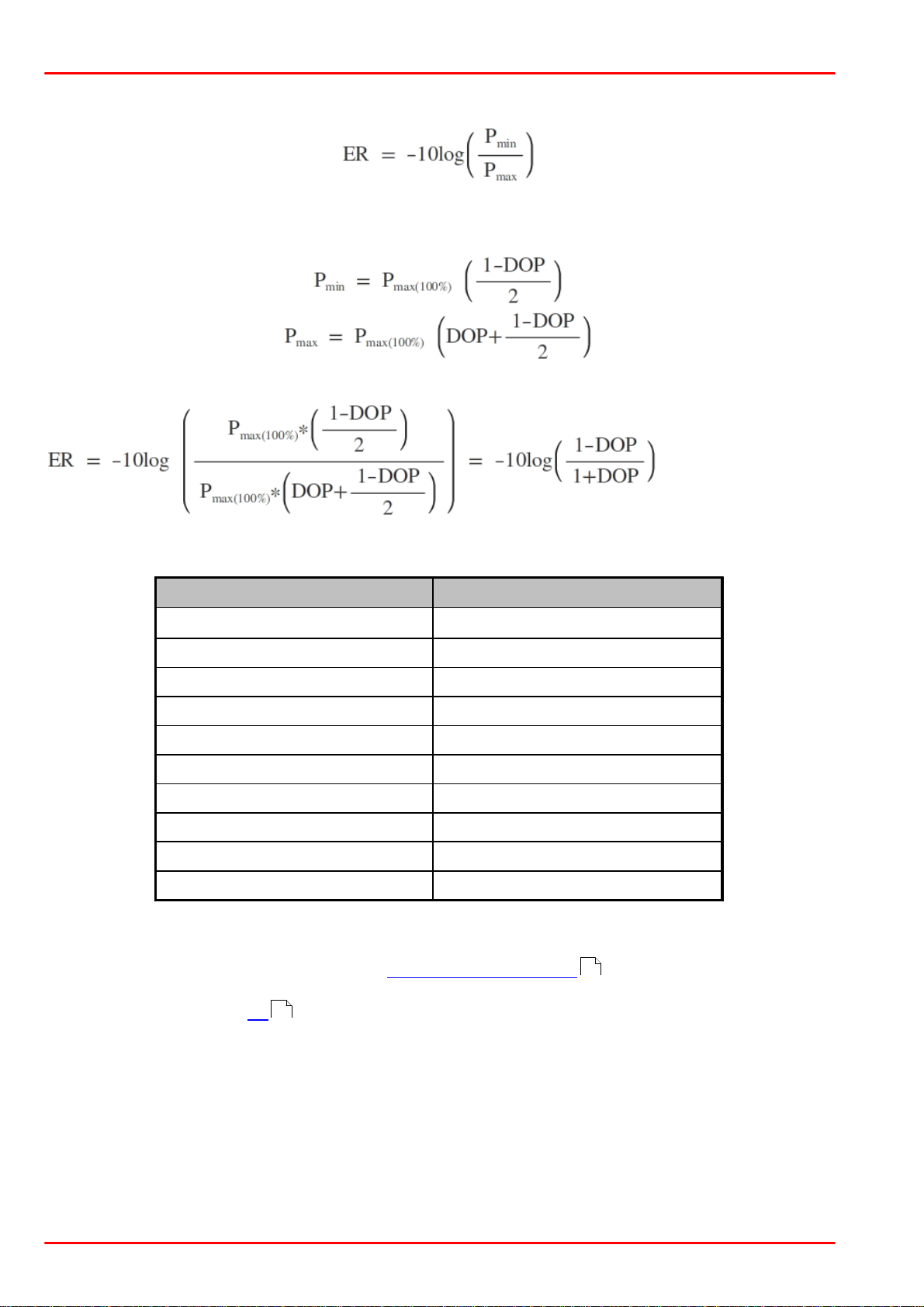
PAX1000

Degree of Polarization [%]

Extinction Ratio [dB]

100

99.998

50.00

99.99

43.01

99.98

40.00

99.95

36.02

99.90

33.01

99.5

26.01

99.0

22.99

98.0

19.96

90.0

12.79

The ER at 100% polarized light (DOP=100%) can be expressed as

For a lower degree of polarization DOP, the maximum and minimum normalized power will change:

The extinction ratio of strongly polarized light with a DOP < 100% can be written then:

The following table lists ERs calculated for different DOPs between 90% and 100%. This demonstrates that the impact of the DOP on the ER of linearly polarized light can be significant.

This illustrates the importance of correcting the ER measurements made by the polarimeter to take into account DOP. Working with the measurement example , the correction for DOP can

be made to the value of ER that was previously corrected for ellipticity. That corrected value was 19.93 dB (Equation [1] ).

Assuming a DOP < 100%, an equation to correct for DOP can be derived as follows.

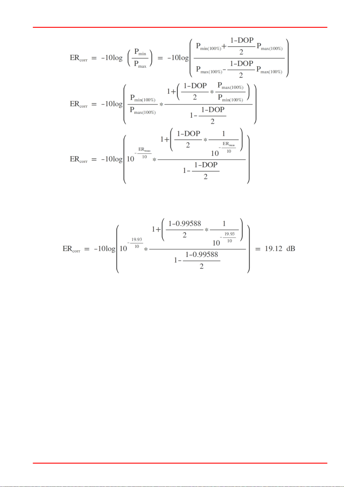
8 Tutorial

The degree of polarization was determined to be 99.588%, and this value was used to correct the ER value for DOP. Using the numbers given in this measurement example, the corrected value of ER is:

Summarize

· Using the polarimeter, an ER of 21.51 dB was measured.

· The ER value corrected for ellipticity (the center ellipticity was measured to be -0.95°) was

19.93 dB.

· Taking into account the measured DOP of 99.588 %, the corrected for center ellipticity

and DOP extinction ratio is 19.12 dB. Note: This is the ER that would have been measured by an instrument, such as the Thorlabs GmbH ERM100, that uses the spinning analyzer technique.

The difference between the uncorrected and the fully corrected ER measurement is more than 2 dB. When comparing ER measurements made by polarimeters and instruments using the spinning analyzer technique, it is necessary to correct the polarimeter's ER measurements for both ellipticity and DOP.

The PAX1000 ER measurement software allows the user to correct the ER measurement result for center ellipticity or DOP or both.

PAX1000

Optical Parameters 1)

Wavelength Range

PAX1000VIS PAX1000IR1 PAX1000IR2

400 nm to 700 nm 600 nm to 1080 nm 900 nm to 1700 nm

Dynamic Range

-60 dBm to +10 dBm

Sampling Rate

Maximum 2) Default

400 Samples / s

30 Samples / s

Measurable SOP States

full Poincaré Sphere

Azimuth Accuracy 3)

±0.25 °

Ellipticity Accuracy

±0.25 °

DOP Accuracy

±1.0 %

Input Fiber Connector

FC/PC

Free Space Aperture

Ø 3mm

Maximum Input Beam Divergence

2 °

General

Interface

USB 2.0

Power Supply

Via USB interface

External Power Supply 15.0 V / 1.2 A DC 4)

Operating Temperature Range 5)

+5 to +40 °C

Storage Temperature Range

-40 to +70 °C

Dimensions (W x H x D)

51.0 mm x 55.0 mm x 56.3 mm (2.01 in x 2.17 in x 2.22 in)

Weight

0.28 kg

Warm-up time for rated accuracy

15 min

9 Appendix

9.1 Technical Data

) All polarization specifications are valid for power range from -40 dBm to +3 dBm.

) One sample per half turn and 200 Hz motor drive speed; with connected external power supply.

) For any SOP with -30° < ellipticity < 30°.

) Required for high-speed measurements; included with the PAX1000

) non-condensing

All technical data are valid at 23 ± 5°C and 45 ± 15% rel. humidity (non condensing).

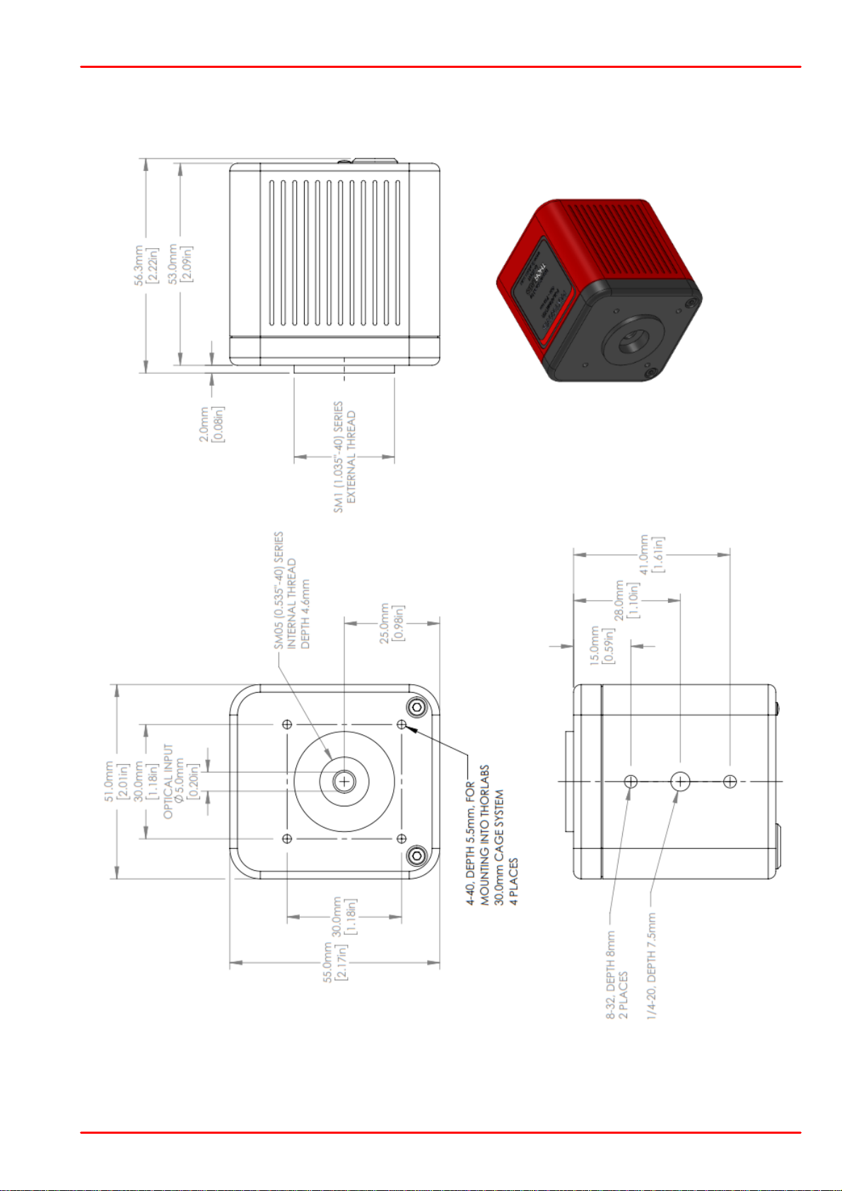
9.2 Dimensions

Dimensions PAX1000xxx (Imperial Version)

9 Appendix

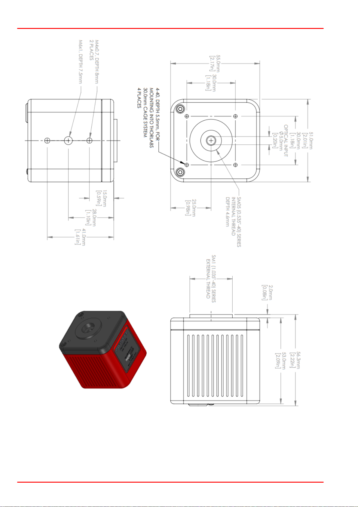
PAX1000

Dimensions PAX1000xxx/M (Metric Version)

9.3 Certifications and Compliances

9 Appendix

PAX1000

9.4 Warranty

Thorlabs GmbH warrants material and production of the PAX1000 for a period of 24 months starting with the date of shipment. During this warranty period Thorlabs GmbH will see to defaults by repair or by exchange if these are entitled to warranty.

For warranty repairs or service the unit must be sent back to Thorlabs GmbH. The customer will carry the shipping costs to Thorlabs GmbH, in case of warranty repairs Thorlabs GmbH will carry the shipping costs back to the customer.

If no warranty repair is applicable the customer also has to carry the costs for back shipment. In case of shipment from outside EU duties, taxes etc. which should arise have to be carried by

the customer. Thorlabs GmbH warrants the hard- and/or software determined by Thorlabs GmbH for this unit

to operate fault-free provided that they are handled according to our requirements. However, Thorlabs GmbH does not warrant a fault free and uninterrupted operation of the unit, of the software or firmware for special applications nor this instruction manual to be error free. Thorlabs GmbH is not liable for consequential damages.

Restriction of Warranty

The warranty mentioned before does not cover errors and defects being the result of improper treatment, software or interface not supplied by us, modification, misuse or operation outside the defined ambient stated by us or unauthorized maintenance.

Further claims will not be consented to and will not be acknowledged. Thorlabs GmbH does explicitly not warrant the usability or the economical use for certain cases of application.

Thorlabs GmbH reserves the right to change this instruction manual or the technical data of the described unit at any time.

9 Appendix

9.5 Copyright and Exclusion of Reliability

Thorlabs GmbH has taken every possible care in preparing this document. We however assume no liability for the content, completeness or quality of the information contained therein. The content of this document is regularly updated and adapted to reflect the current status of the hardware and/or software. We furthermore do not guarantee that this product will function without errors, even if the stated specifications are adhered to.

Under no circumstances can we guarantee that a particular objective can be achieved with the purchase of this product.

Insofar as permitted under statutory regulations, we assume no liability for direct damage, indirect damage or damages suffered by third parties resulting from the purchase of this product. In no event shall any liability exceed the purchase price of the product.

Please note that the content of this document is neither part of any previous or existing agreement, promise, representation or legal relationship, nor an alteration or amendment thereof. All obligations of Thorlabs GmbH result from the respective contract of sale, which also includes the complete and exclusively applicable warranty regulations. These contractual warranty regulations are neither extended nor limited by the information contained in this document. Should you require further information on this product, or encounter specific problems that are not discussed in sufficient detail in the document, please contact your local Thorlabs GmbH dealer or system installer.

PAX1000

Crossed out

"Wheelie Bin" symbol

9.6 Thorlabs 'End of Life' Policy

As required by the WEEE (Waste Electrical and Electronic Equipment Directive) of the European Community and the corresponding national laws, Thorlabs GmbH offers all end users in the EC the possibility to return “end of life” units without incurring disposal charges.

This offer is valid for Thorlabs GmbH electrical and electronic equipment

· sold after August 13th 2005

· marked correspondingly with the crossed out “wheelie bin” logo (see figure below)

· sold to a company or institute within the EC

· currently owned by a company or institute within the EC

· still complete, not disassembled and not contaminated

As the WEEE directive applies to self contained operational electrical and electronic products, this “end of life” take back service does not refer to other Thorlabs GmbH products, such as

· pure OEM products, that means assemblies to be built into a unit by the user (e. g. OEM laser driver cards)

· components

· mechanics and optics

· left over parts of units disassembled by the user (PCB’s, housings etc.).

Waste treatment on your own responsibility

If you do not return an “end of life” unit to Thorlabs GmbH, you must hand it to a company specialized in waste recovery. Do not dispose of the unit in a litter bin or at a public waste disposal site.

WEEE Number (Germany) : DE97581288

Ecological background

It is well known that waste treatment pollutes the environment by releasing toxic products during decomposition. The aim of the European RoHS Directive is to reduce the content of toxic substances in electronic products in the future.

The intent of the WEEE Directive is to enforce the recycling of WEEE. A controlled recycling of end-of-life products will thereby avoid negative impacts on the environment.

9.7 List of Acronyms

ADC Analog-to-Digital Converter DC Direct Current DFB Distributed Feedback (laser) DOP Degree of Polarization ER Extinction Ratio FBG Fiber Bragg Grating FFT Fast Fourier Transformation GUI Graphical User Interface LED Light Emitting Diode LTM Long Term Measurement MMF Multi-mode Fiber PC Personal Computer PMD Polarization Mode Dispersion PMF Polarization-maintaining Fiber

9 Appendix

QWP Quarter Waveplate SMF Single-mode Fiber SOP State of Polarization USB Universal Serial Bus WP Waveplate

PAX1000

9.8 Literature

[1]Jones Calculus (https://en.wikipedia.org/wiki/Jones_calculus ; WP:CC BY-SA ) [2]Solid Angle (https://en.wikipedia.org/wiki/Solid_angle; WP:CC BY-SA) [3]Serge Huard, Polarization of Light, Wiley, New York, 1997. [4]Eugene Hecht, Optics, Addison Wesley, New York, 2016. [5]Christian Brosseau, Fundamentals of Polarized Light: A Statistical Optics Approach, Wiley,

New York, 1998.

9.9 Thorlabs Worldwide Contacts

USA, Canada, and South America

Thorlabs, Inc. 56 Sparta Avenue Newton, NJ 07860 USA Tel: 973-300-3000 Fax: 973-300-3600

www.thorlabs.com www.thorlabs.us (West Coast)

Email: sales@thorlabs.com Support: techsupport@thorlabs.com

UK and Ireland

Thorlabs Ltd. 1 Saint Thomas Place, Ely Cambridgeshire CB7 4EX United Kingdom Tel: +44-1353-654440 Fax: +44-1353-654444

www.thorlabs.com

Email: sales.uk@thorlabs.com Support: techsupport.uk@thorlabs.com

Europe

Thorlabs GmbH Hans-Böckler-Str. 6 85221 Dachau Germany Tel: +49-8131-5956-0 Fax: +49-8131-5956-99

www.thorlabs.de

Email: europe@thorlabs.com

Scandinavia

Thorlabs Sweden AB Bergfotsgatan 7 431 35 Mölndal Sweden Tel: +46-31-733-30-00 Fax: +46-31-703-40-45

www.thorlabs.com

Email: scandinavia@thorlabs.com

France

Thorlabs SAS 109, rue des Côtes 78600 Maisons-Laffitte France Tel: +33-970 444 844 Fax: +33-825 744 800

www.thorlabs.com

Email: sales.fr@thorlabs.com

Brazil

Thorlabs Vendas de Fotônicos Ltda. Rua Riachuelo, 171 São Carlos, SP 13560-110 Brazil Tel: +55-16-3413 7062 Fax: +55-16-3413 7064

www.thorlabs.com

Email: brasil@thorlabs.com

Japan

Thorlabs Japan, Inc. 3-6-3 Kitamachi Nerima-ku, Tokyo 179-0081

Japan

Tel: +81-3-6915-7701 Fax: +81-3-6915-7716

www.thorlabs.co.jp

Email: sales@thorlabs.jp

China

Thorlabs China Room A101, No. 100 Lane 2891, South Qilianshan Road Putuo District Shanghai 200331 China Tel: +86-21-60561122 Fax: +86-21-32513480

www.thorlabs.com

Email: chinasales@thorlabs.com

9 Appendix

PAX1000

Index

About Add Virtual Device Alignment Assistance

Basic Sample rate Bulk Optics Button Default

Clear Data Color Setup Correction ER Measurement

Default Device Color Device Information Device Settings

(measurement) Device Settings

(Polarimeter) Devices & Measurements Diagram Options

Ellipse ER Measurement Setup ER Measurement Tool ER Measurement Wizard Error Messages Exit Extinction Ratio

Extinction Ratio Measurement

Fiber Fiber Optics First Steps

22 20 25

24 71 20

31 31 75

20 20 20 20

20 20

60 36 41 38 51 17

36, 38, 41,

63, 73, 75

63 71 14

GUI

Help

Installing Software

Long Term Measurement LTM Settings

Measurement Technique Measurement Value Table Menu View Microsoft .Net Mounting Multiple Devices

NI-VISA Runtime

Open Open / Save Operating Elements Operating Mode Operating Principle

Pan Pause / Run Pin Poincaré Sphere Polarization Controller Polarization Ellipse Polarization in Fibers Polarization Measurement Polarization of Light

Polarization Parameters Polarization Scrambler

15, 22

34 34

67 27 22

4 8

17 17

31 20 15

29, 62

29, 60

63 67

53, 58, 60,

62, 63, 65

65 72

9 Appendix

Polarization Transformation Power Range Print Product License

Requirements Reset All Reset Layout Ribbons Rotating Waveplate Rotating Waveplate

Technique

Sample rate Save Save Configuration Save Measurement Scan USB Scope Mode Screenshot Settings SOP Reference Status Bar

71 20

15, 17

4 20, 21 22, 26

15 67 67

24 15 17 17 20 31

17 20, 24 27, 29 15, 23

Theme Tool Bar Trace Setup Troubleshooting

Version Views Virtual Device

Wavelength Window Settings Workspace

Zoom and Pan

www.thorlabs.com

THORLABS PAX1000 Operation Manual

Specifications and Main Features

Frequently Asked Questions

User Manual

1 General Information

1.1 Safety

1.2 Ordering Codes and Accessories

1.3 Requirements

2 Getting Started

2.1 Parts List

2.2 Operating Principle

2.3 Operating Elements

2.4 Mounting

2.5 Installing Software

2.6 First Steps

3 Graphical User Interface (GUI)

3.1 General

3.2 GUI Overview

3.3 Menu File

3.4 Menu Device

3.5 Menu View

3.6 Menu Tools

3.7 Menu Help

3.8 Status Bar

4 PAX1000 Settings

5 Operating Instruction

5.1 Alignment Assistance

5.2 PAX1000 Measurements

5.2.1 Measurement Value Table

5.2.2 Polarization Ellipse

5.2.3 Poincaré Sphere

5.2.4 Scope Mode

5.2.5 Long Term Measurement

5.2.5.1 Settings

5.2.5.2 Measurement

5.2.6 Extinction Ratio Measurement

5.2.6.1 ER Measurement Wizard

5.2.6.2 ER Measurement Tool

5.2.7 Virtual Device

5.2.8 Multiple Devices

6 Write Your Own Application

6.1 32 Bit Operating Systems

6.2 64 Bit Operating Systems

7 Maintenance and Service

7.1 Version Information

7.2 Troubleshooting

8 Tutorial

8.1 Polarization of Light

8.1.1 The Nature of Polarization

8.1.2 Handedness of Polarization

8.1.3 Mathematical Representation of an Electromagnetic Wave

8.1.4 Polarization Ellipse

8.1.5 Poincaré Sphere

8.1.6 Polarization in Fibers

8.1.7 Polarization Parameters - Definitions

8.2 Polarization Measurement Technique

8.2.1 Rotating Waveplate Technique

8.3 Polarization Control and Transformation

8.3.1 Bulk Optics

8.3.2 Fiber Polarization Controllers

8.3.3 Fiber Polarization Scrambler

8.4 Extinction Ratio Measurement on PM Fibers

8.4.1 Definition

8.4.2 Measurement

8.4.3 Correction of the Polarimeter ER Measurements

9 Appendix

9.1 Technical Data

9.2 Dimensions

9.3 Certifications and Compliances

9.4 Warranty

9.5 Copyright and Exclusion of Reliability

9.6 Thorlabs 'End of Life' Policy

9.7 List of Acronyms

9.8 Literature

9.9 Thorlabs Worldwide Contacts