THORLABS CCS Series, CCS100/M, CCS175/M, CCS200, CCS100 Operation Manual

...

Download

Spectrometer

CCS Series Spectrometer Operation Manual

2018

Version: Date:

2.1 09-Jul-2018

Contents

Foreword

1 General Information 4

2 Installation 7

3 Getting Started 13 4 Operating Instruction 15

164.1 Main Menu

164.1.1 File

194.1.2 Sweep

224.1.3 Display

254.1.4 Level

264.1.5 Marker

41.1 Safety

61.2 Ordering Codes and Accessories

61.3 Requirements

72.1 Parts List

82.2 Installing Software

264.1.5.1 Movable Markers

284.1.5.2 Fixed Markers

304.1.6 Analysis

304.1.6.1 Peak Track Analysis

324.1.6.2 Color Analysis

334.1.6.3 Statistics

344.1.6.4 Long Term Analysis

374.1.7 Math

434.1.8 Setup

434.1.8.1 Tab Active Device

484.1.8.2 Tab Display

494.1.8.3 Tab Peak Track

504.1.8.4 Tab Reset

504.1.9 Help

514.2 Settings Bar

524.3 Trace Controls

5 Write Your Own Application 55

565.1 NI VISA Instrument driver 32bit on 32bit systems

585.2 NI VISA Instrument driver 32bit on 64bit systems

605.3 NI VISA Instrument driver 64bit on 64bit systems

6 Maintenance and Service 62

626.1 Version Information

636.2 Troubleshooting

7 Appendix 64

647.1 Technical Data

657.2 Dimensions

667.3 Tutorial

707.4 Shortcuts Used in OSA Software

717.5 Certifications and Compliances

727.6 Warranty

737.7 Copyright and Exclusion of Reliability

747.8 Thorlabs 'End of Life' Policy (WEEE)

757.9 List of Acronyms

767.10 Thorlabs Worldwide Contacts

We aim to develop and produce the best solution for your application in the field of optical measurement technique. To help us to live up to your expectations and improve our products permanently we need your ideas and suggestions. Therefore, please let us know about possible criticism or ideas. We and our international partners are looking forward to hearing from you.

Thorlabs GmbH

Warning

Sections marked by this symbol explain dangers that might result in personal injury or death. Always read the associated information carefully, before performing the indicated procedure.

Attention

Paragraphs preceded by this symbol explain hazards that could damage the instrument and the connected equipment or may cause loss of data.

Note

This manual also contains "NOTES" and "HINTS" written in this form.

Please read these advices carefully!

CCS Series Spectrometer

1 General Information

The CCS Series Spectrometer is designed for general laboratory use. Integrated routines allow averaging, smoothing, peak indexing, as well as saving and recalling data sets.

Attention

Do not connect the CCS Series Spectrometer to a PC prior to installingh the OSA-SW Application! The installation package includes CCS Series Spectrometer specific drivers and software that must be installed before the CCS Series Spectrometer is connected to the PC for the first time.

A troubleshooting section and detailed specifications of the various components are provided in this manual. The description of the instrument driver commands can be found in the VXIpnp VISA instrument driver package.

Application software OSA-SW OSA-SW is an acronym for "Optical Spectrum Analyzer Software". This software can be used for

acquiring direct, transmittance and absorbance measurements in conjunction with Thorlabs' optical spectrum analyzers and CCD spectrometers.

After the installation, the software is able to communicate with all Thorlabs CCD based CCS Series Spectrometers and OSA20x Optical Spectrum Analyzers. Additionally, a number of virtual devices are included to demonstrate the functionality of OSA-SW: five for OSA20x Analyzers and one for CCS spectrometers.

1.1 Safety

Attention

The safety of any system incorporating the equipment is the responsibility of the assembler of the system.

All statements regarding safety of operation and technical data in this instruction manual will only apply when the unit is operated correctly as it was designed for.

The CCS Series Spectrometer must not be operated in explosion endangered environments!

Do not obstruct the air ventilation slots in the housing! Do not remove covers! Do not open the cabinet. There are no parts serviceable by the operator inside! This precision device is only serviceable if properly packed into the complete original

packaging including the plastic foam sleeves. If necessary, ask for replacement packaging.

Refer servicing to qualified personnel! Only with written consent from Thorlabs may changes to single components be made or

components not supplied by Thorlabs be used.

Attention

The following statement applies to the products covered in this manual, unless otherwise specified herein. The statement for other products will appear in the accompanying documentation.

1 General Information

Note This equipment has been tested and found to comply with the limits for a Class A

digital device, pursuant to part 15 of the FCC Rules. These limits are designed to provide reasonable protection against harmful interference when the equipment is operated in a commercial environment. This equipment generates, uses, and can radiate radio frequency energy and, if not installed and used in accordance with the instruction manual, may cause harmful interference to radio communications. Operation of this equipment in a residential area is likely to cause harmful interference in which case the user will be required to correct the interference at his own expense.

Users that change or modify the product described in this manual in a way not expressly approved by Thorlabs (party responsible for compliance) could void the user’s authority to operate the equipment.

Thorlabs is not responsible for any radio television interference caused by modifications of this equipment or the substitution or attachment of connecting cables and equipment other than those specified by Thorlabs. The correction of interference caused by such unauthorized modification, substitution or attachment will be the responsibility of the user.

The use of shielded I/O cables is required when connecting this equipment to any and all optional peripheral or host devices. Failure to do so may violate FCC and ICES rules.

Attention

Mobile telephones, cellular phones or other radio transmitters are not to be used within the range of three meters of this unit since the electromagnetic field intensity may then exceed the maximum allowed disturbance values according to IEC61326-1.

This product has been tested and found to comply with the limits according to IEC613261 for using connection cables shorter than 3 meters (9.8 feet).

CCS Series Spectrometer

Ordering code

Short description CCS100(/M) 1)

CCS spectrometer, 350 - 700 nm

CCS175(/M) 1)

CCS spectrometer, 500 - 1000 nm

CCS200(/M) 1)

CCS spectrometer, 200 - 1000nm

M14L01

1 m SMA MMF Patch Cable, 50µm / 0.22 NA (to CCS100 and CCS175)

FG200UCC

1 m SMA MMF Patch cable, 200µm / 0.22 NA, High OH (to CCS200)

CVH100; CVH100/M

Cuvette holder (imperial and metric versions)

1.2 Ordering Codes and Accessories

) CCSxxx = imperial version, mounting holes 1/4-20;

CCSxxx/M = metric version, mounting holes M6x1

Attention

Make sure to use your CCS spectrometer only with the included fiber (see above table). If using a different fiber, the Amplitude Correction Calibration will be affected!

1.3 Requirements

These are the requirements to the PC intended to be used for remote operation of the CCS Series Spectrometer.

Minimum Hardware and Software Requirements

• Operating System: Windows Vista or Windows 7 (32 or 64 bit)

• Free USB 2.0 high speed port (Notice that a USB 1.1 port cannot be used)

• Processor: Intel Pentium 4 or AMD Athlon 64 3000+

• 2.0 GB RAM

• .NET framework 4.0 or higher

Recommended Hardware and Software Requirement

• Operating System: Windows 7, 64 bit

• Free USB 2.0 high speed port (Notice that a USB 1.1 port cannot be used)

• Processor: Intel Core i5 or AMD Athlon II

• 6.0 GB RAM

• .NET framework 4.0 or higher

Note

Please be aware that the OSA software requires a number of third party software installed on your system. The installer checks for these software components and, if necessary, will install them automatically. You will be notified accordingly.

2 Installation

CCS Series Spectrometer

This CCS Series Spectrometer Quick Reference

CD-ROM with application software OSA-SW, drivers and PDF User Manual

USB 2.0 A-B mini cable, 1.5 meters

Optical Fiber, SMA to SMA, 50µm / 0.22 NA, 1 meter (CCS100, CCS175) Quartz Fiber, SMA to SMA, 200µm / 0.22 NA, 1 meter (CCS200)

Trigger Input cable SMB to BNC

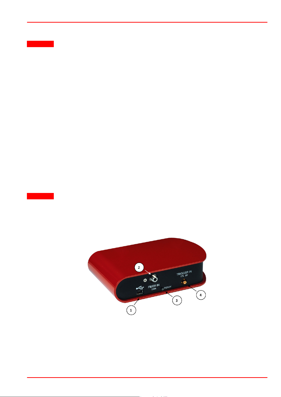
(1)

USB port

(2)

Fiber input (SMA connector)

(3)

Status LED

(4)

Trigger Input (SMB connector)

2 Installation

Attention

Do not connect the CCS Series Spectrometer to a PC prior to install the OSA-SW Application! The installation package includes CCS Series Spectrometer specific drivers and software that must be installed before the CCS Series Spectrometer is connected to the PC for the first time.

2.1 Parts List

Inspect the shipping container for damage. If the shipping container seems to be damaged, keep it until you have inspected the contents and you have inspected the CCS Series Spectrometer mechanically and electrically.

Verify that you have received the following items within the package:

Attention

Make sure to use your CCS spectrometer only with the included fiber (see above table). If using a different fiber, the Amplitude Correction Calibration will be affected.

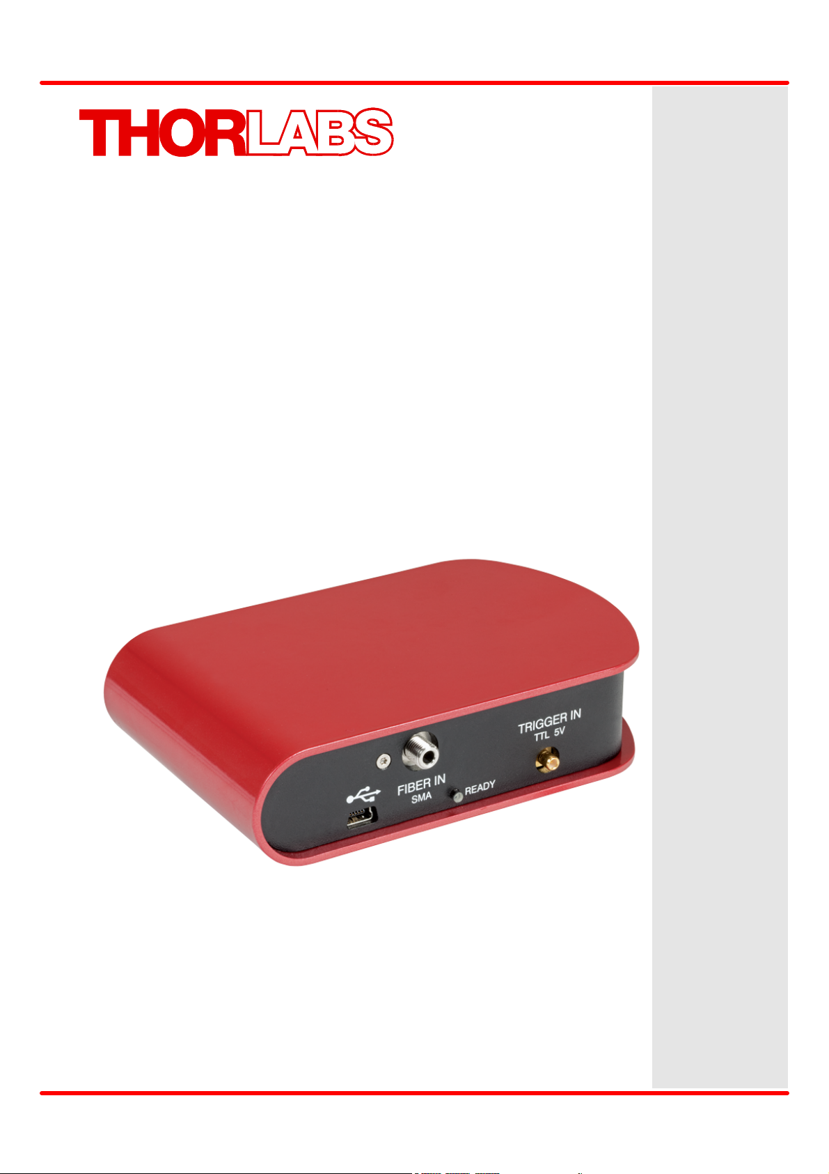
CCS Spectrometer - Ports and Signal LEDs

CCS Series Spectrometer

2.2 Installing Software

Before installing OSA Software, please make sure that no CCS Series Spectrometer is connected. After you insert the OSA Software installation CD an autorun menu will appear (see figure below). If autorun is disabled on your system, you will have to browse the installation CD and run

"[CD-Drive]:\Autorun\Autorun.exe":

Click to "Install Software":

Note

Administrator privileges are required for installation. Please contact your system administrator if you get an error message.

Installation steps are shown below in detail for an installation on a Windows 7© operating system. After selecting "Install Software", the installer checks your system and determines the software components that need to be installed.

2 Installation

Click "Install" to continue. The necessary software components are being installed, followed by installation of device driver software. The installation of all components is described below.

NI VISA installation

Click "I accept...", then "Next>>" to continue:

CCS Series Spectrometer

After NI-VISA Installation, the computer must be restarted. After reboot, the setup wizard restarts automatically and continues to install further software components:

2 Installation

Click "I accept...", then "Next>>" to continue:

CCS Series Spectrometer

Depending on the set up security level, the Installation Wizard might ask to allow to install the driver software:

To finalize the OSA Software installation, the computer must be restarted. Click "Finish" to restart and complete installation.

3 Getting Started

Attention

Do not connect the CCS Series Spectrometer to a PC prior to installing the OSA-SW Application! The installation package includes CCS Series Spectrometer specific drivers and software that must be installed before the CCS Series Spectrometer is connected the first time to the PC.

The initial setup is simple to complete. Following installation of the software, connect the CCS Series Spectrometer to a USB 2.0 port. The operating system recognizes the new hardware and installs the firmware loader and the driver:

Then run the application software OSA-SW either from the desktop icon

1. Click to trace A and make sure that the topics below are checked.

Show

CCS Series Spectrometer

Set as Active

Write

2. Check that the connected spectrometer is recognized. If not, click to "Scan USB"

3. Apply an optical input signal to the fiber input. Increase the integration time until the spectrum is

displayed. A right click into the data display area zooms in the intensity axis to it's best fit to the spectrum.

Note

If you are using a CCS200 broadband spectrometer and a continuous spectrum (e.g. of a white light lamp) shall be measured, please note the following recommendation:

Due to the eccentricity between the fiber core and the ferrule of the delivered FG200UCC MMF and the geometry of the input slit of the spectrometer, the displayed spectral intensity may vary when the SMA connector of the fiber is rotated within the input receptacle of the CCS200. Please find the maximum intensity by rotation and then fix the fiber connector with the lock bush. This ensures best measurement results.

The remainder of this manual is devoted to the setup procedure and features of the CCS Series Spectrometer.

4 Operating Instruction

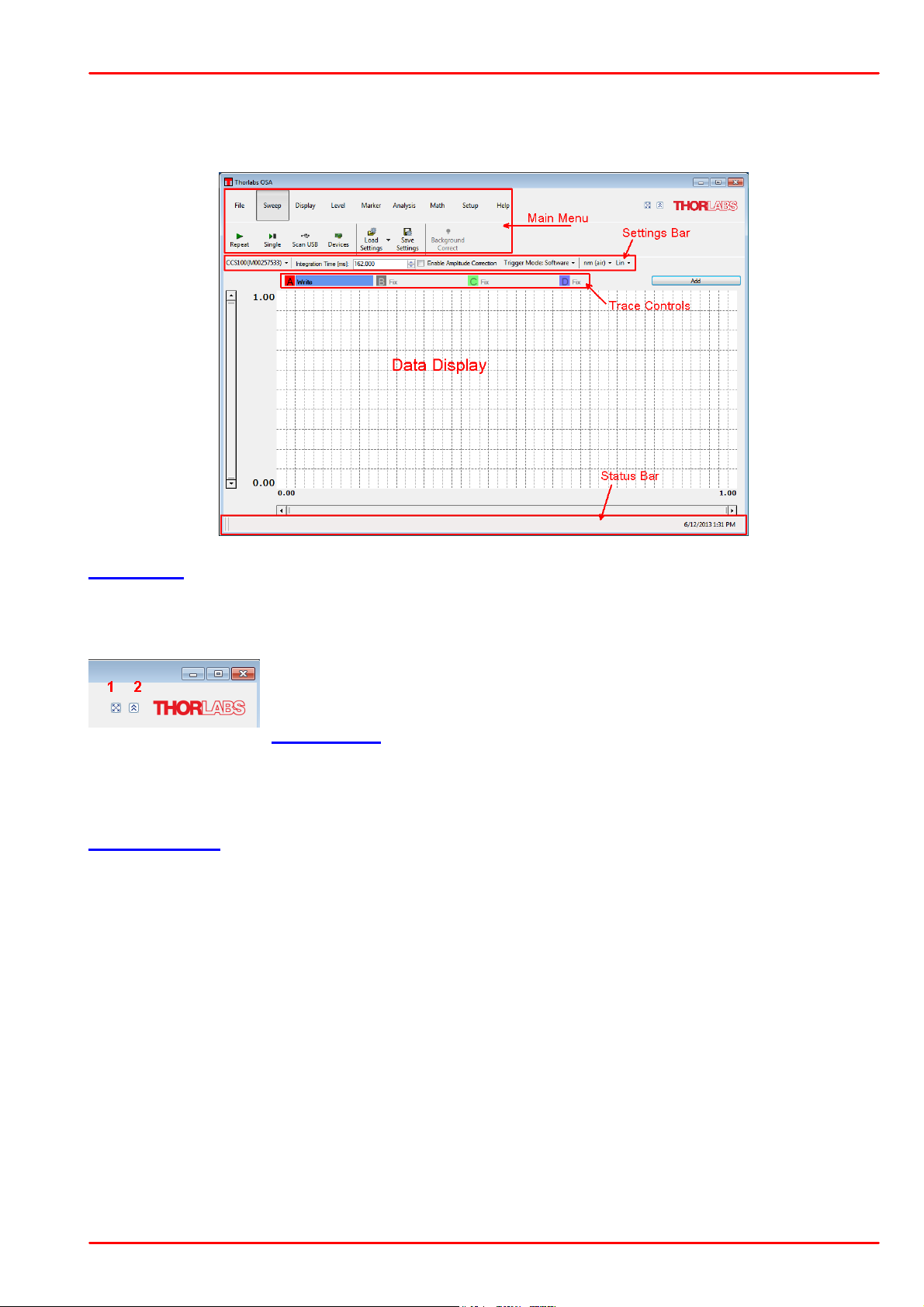
The OSA Software GUI is divided into 5 functional areas:

4 Operating Instruction

Main Menu

Depending on the selected main topic in the upper part of the bar, the lower bar will show particular sub-topics. These topics are explained with references to the section explaining their functionality in detail.

The GUI can be expanded to full size using button 1, button 2 minimizes the main menu.

Settings Bar

The Settings Bar offers quick access to important control features: The active spectrometer can be selected; the integration time, amplitude correction, trigger mode and display properties can be set.

Trace Controls

The OSA software GUI displays spectra using multiple "Traces". For each trace, both the settings of the GUI and the used spectrometer are saved. The trace can be used for numerous functions and calculations, hence traces are a powerful tool for measurement and data handling. Up to 26 traces, marked with A to Z, can be enabled. To the right of the trace letter (“A”, “B”, etc.) the update option for the trace is displayed. This option determines what will happen with the trace during the next data acquisition. Only one trace can be active, as shown above in the screenshot of trace A. The active trace's update option is shown with a blue background.

Data Display

Here the acquired spectral data are displayed in graphic view. The intensity and the wavelength axes can be zoomed and panned numerically via a dialog or using the graphic zoom bars. Additionally, the intensity axis can be displayed in linear or logarithmic scale.

Status Bar

The status bar displays information about the measurement status and the current date and time.

CCS Series Spectrometer

4.1 Main Menu

In the next sections the main menu items are explained in detail:

File Menu

Display Menu

Sweep Menu

Level Menu

Marker Menu

Analysis Menu

Math Menu

Setup Menu

Help Menu

There are a number of keyboard shortcuts listed in the Appendix.

4.1.1 File

The File Menu allows to save, load, print and delete spectra from the GUI.

Clear All

clears all traces in the display. Save Trace (shortcut: Ctrl + S) Saves only the currently active trace, all other traces are ignored.

Possible file formats: Thorlabs OSA spectrum files (*.spf2); Comma Separated Values (*.csv)

Note

For details on the supported spectrum file formats, see Tutorial. Save All (shortcut: Ctrl + Shift + S) Saves all shown traces.

Possible file formats: Thorlabs OSA spectrum files (*.spf2) only.

Export Trace

Exports the currently active trace for use in other software environment. Possible export formats: Galactic (*.spc), JCAMP-DX (*.jdx), Matlab level 5 (*.mat). Additionally,

the trace can be exported to a text file (*.txt) and to ZIP archives (*.txt.zip; *.csv.zip). Load (shortcut: Ctrl +O) Loads previously saved spectrum file(s) to the graphic diagram into free traces. The trace (traces)

is (are) loaded in the next free trace (traces).

Note

Numbers in the file to be loaded, must have the standard format - decimal point, not a decimal comma.

4 Operating Instruction

Save Image

Saves the current view of the data display as an image. This allows you to quickly save a measurement result for documentation purposes.

Print (shortcut: Ctrl +P) Prints the current view of the data display to a Windows printer.

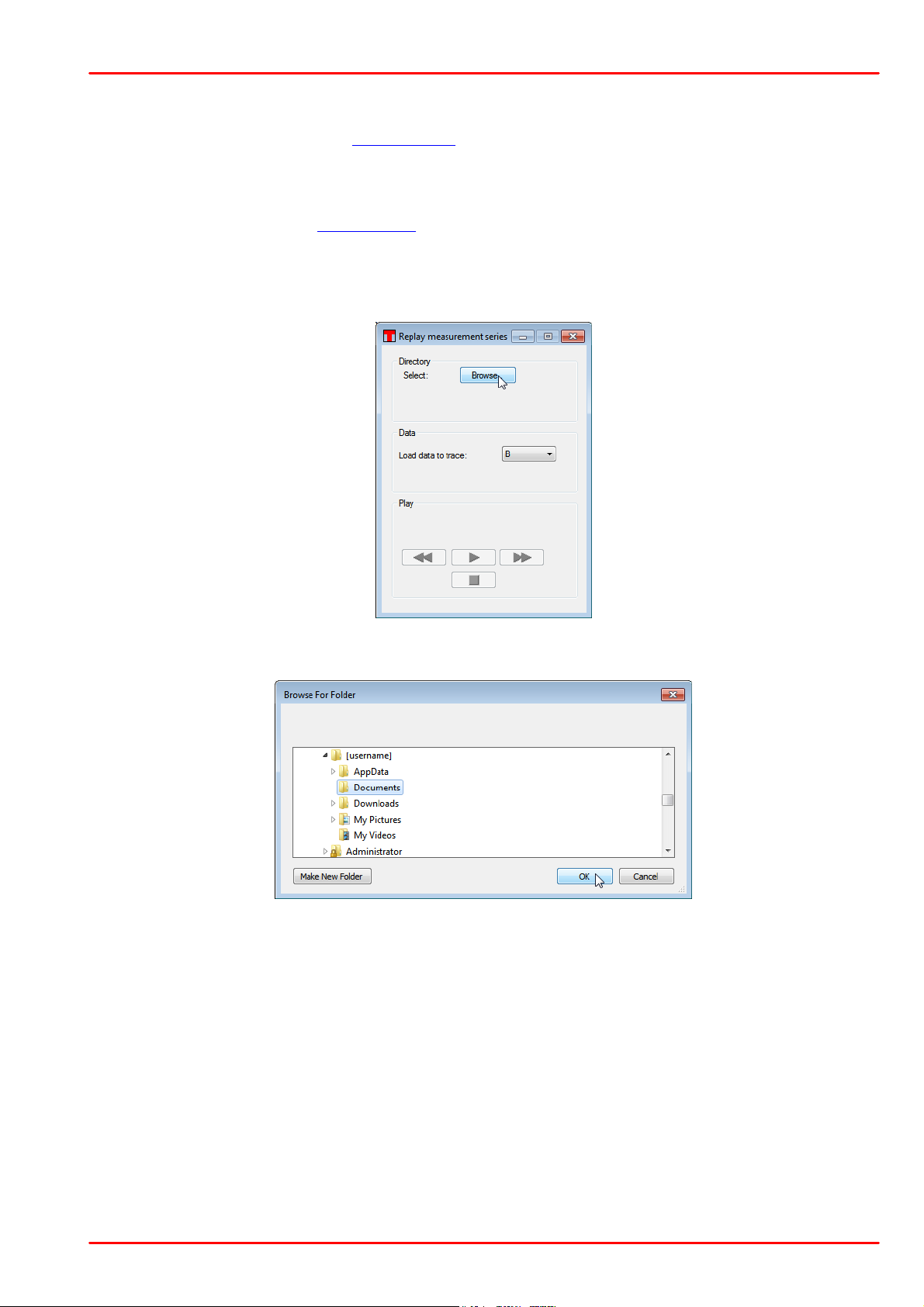
Replay

Replays a series of saved single traces. This button opens a dialog window.

Click Browse

Select the folder with the saved *.spf2 files, then click OK.

CCS Series Spectrometer

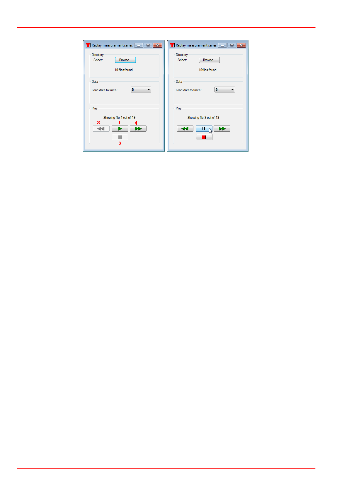
You may change the trace to load the data to. The "Play" button (1) loads the located files sequentially like a slide show. The replay can be stopped (button 2) or paused. Buttons 3 and 4 allow you to manually load the spectrum files.

4 Operating Instruction

4.1.2 Sweep

The Sweep menu controls start, stop and the type of spectrum sweep. Settings that were made for the sweep can be saved and loaded. Additional features of the Sweep menu are enabling a background correction, scanning the USB interface for new devices and selecting them for a sweep.

Repeat (shortcut Ctrl + R) Starts repeated spectrum measurements. The sweep is executed and a status bar message

informs about the started continuous acquisition and the integration time of the recent spectrum. The repeated sweep is terminated by pressing the Stop button.

Single (shortcut Ctrl + N) Starts a single spectrum acquisition with the given integration time.

Scan USB

Scans the USB interface for connected devices.

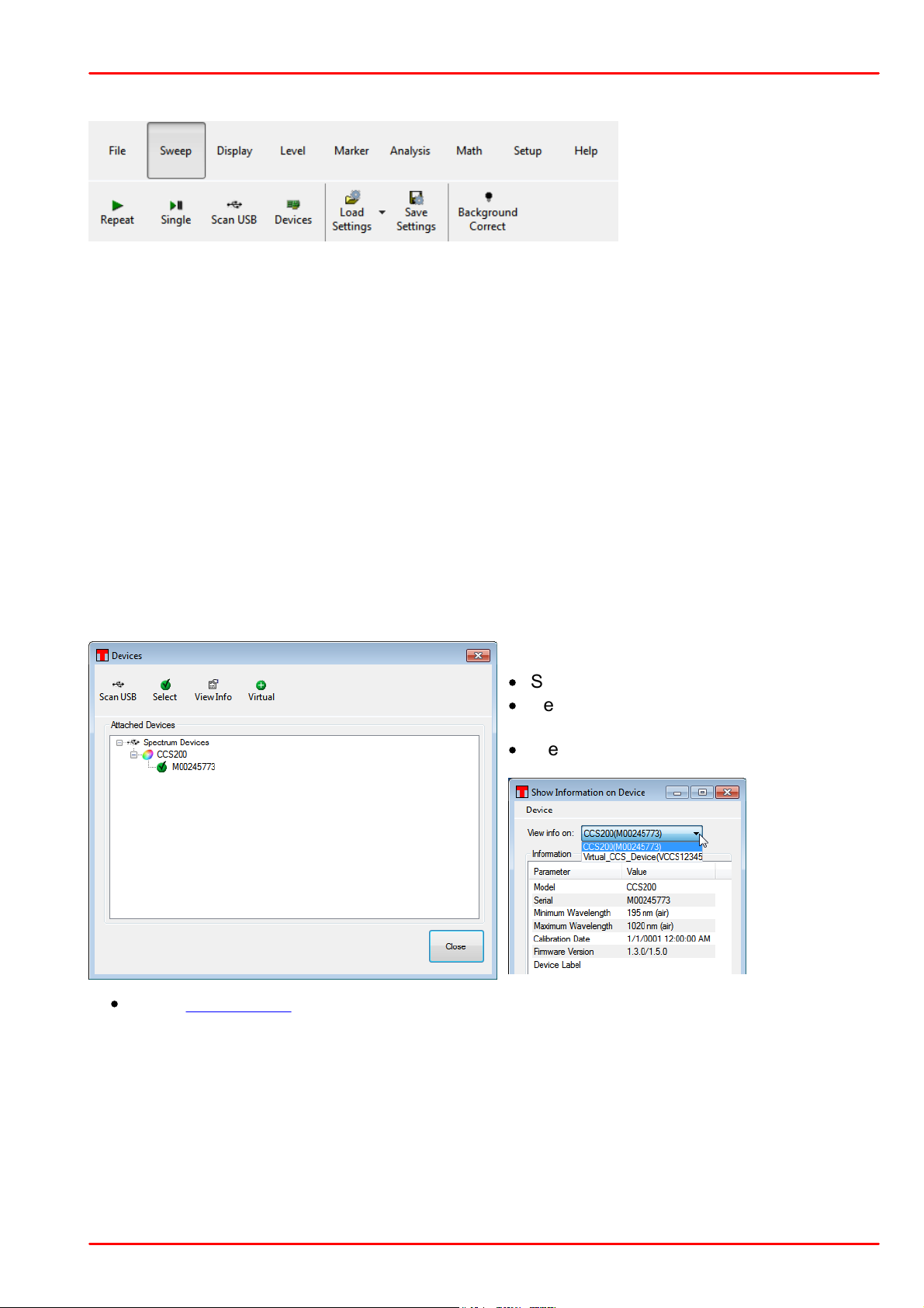
Devices

Opens the device dialog:

Functions:

Scan USB for connected devices

Select from the list a device to be the active

one

View Info about the selected device

Add a virtual device.

CCS Series Spectrometer

Switch between connected instruments

If more than one spectrum device is connected and recognized, you can switch between them by using the Select button in Device menu or by using the the quick select drop down menu in the

Settings bar:

Note

Prior to switching the active instrument, please make sure that the spectrum acquisition is stopped!

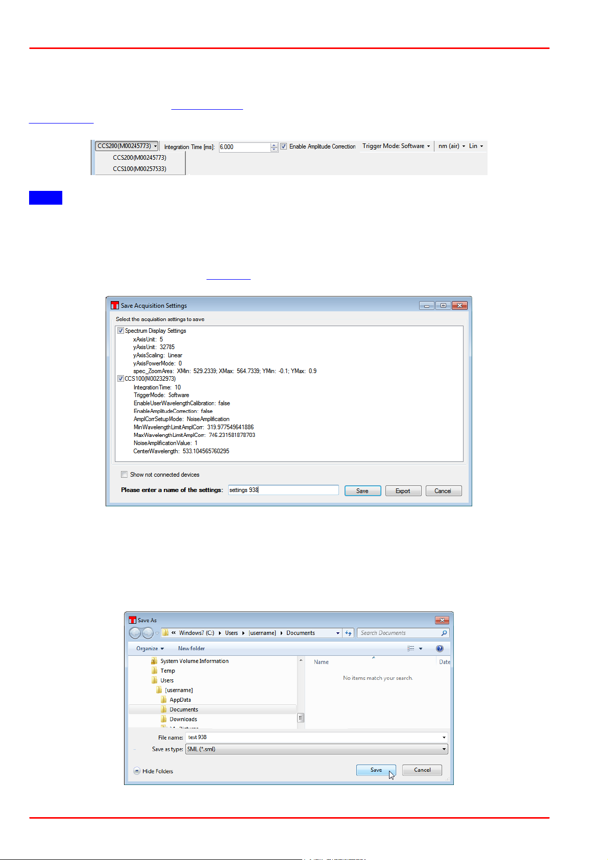
Save Settings

The actual application configuration - the settings of the spectrum display and / or of the active spectrometer - can be saved to a SML file. Click the Save Settings button to open the dialog:

Enter a name and click the Save button. The configuration is saved to

C:\Users\[username] \AppData\Local\Thorlabs\OSA\Settings_YYYY_MM_DD_hh_mm_ss.sml

The above entered name of the settings is written to the XML code. Alternatively, the current application configuration can be saved to any other required location by pressing the Export button:

Select the desired file location, enter a valid file name and press Save.

4 Operating Instruction

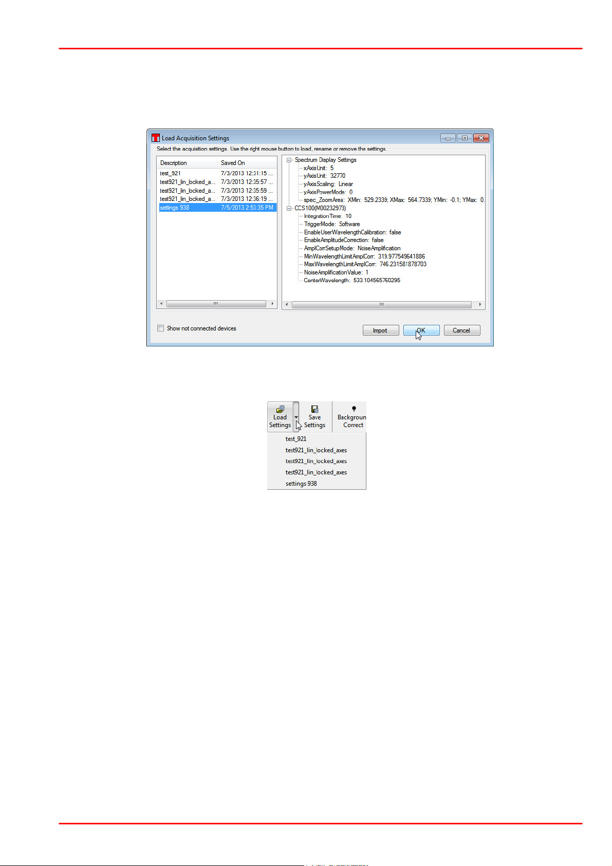
Load Settings

Previously saved configurations can be loaded (from C:\Users\[username] \AppData\Local\Thorlabs\OSA\) or imported (from any other folder):

Using the drop down arrow, a list of saved (not exported) settings is displayed and can be quickly selected:

Background Correct

When pressing this button, the actual spectrum is saved as background spectrum. Starting from the next spectrum acquisition, the difference between the actual and the background data will be displayed. This feature is useful to eliminate environmental stray light or noise.

CCS Series Spectrometer

4.1.3 Display

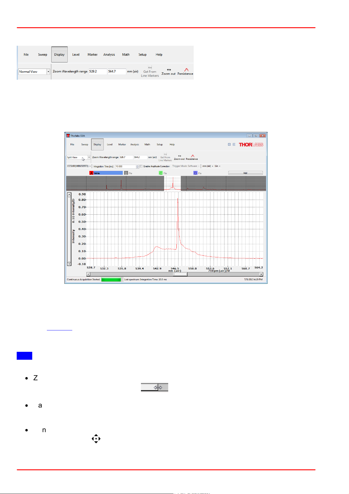
In the Display menu, the wavelength axis display can be configured.

Normal / Split View

The Normal View shows the spectrum display only. The Split View adds an overview that marks the actual zoom window within the entire operating wavelength range of the connected spectrometer:

Zoom Wavelength Range

The zoom wavelength range can be set numerically in the appropriate boxes. As soon as a valid number has been recognized, the display is updated.

If vertical markers are enabled (markers 1 and 2), the display can be zoomed in on the range between the 2 markers ("Get from Line Markers"). "Zoom out" returns the display to the entire operating wavelength of the connected device.

Note

There are several additional methods to zoom and pan wavelength axis of the spectrum display:

Zooming using the X axis scroll bar: Place the mouse pointer over one of the two edges of the scroll bar, the pointer will change to

, click left and drag&drop this edge to achieve

the desired zoom.

Panning using the scroll bar: Place the mouse pointer over the scroll bar, then click and drag&drop the display to the desired position. The wavelength zoom does not change in this case.

Panning using the mouse: Place the mouse pointer into the diagram area and click left, the pointer changes to . Hold the mouse button pressed and move the entire display to the

desired position .

4 Operating Instruction

Zooming using the scroll wheel of the mouse: Place the mouse pointer into the diagram area and click once left mouse button (the pointer changes for the time of pressing left mouse

button to ). Now, using the scroll wheel the zoom factor can be set visually.

Zooming using the X axis properties dialog.

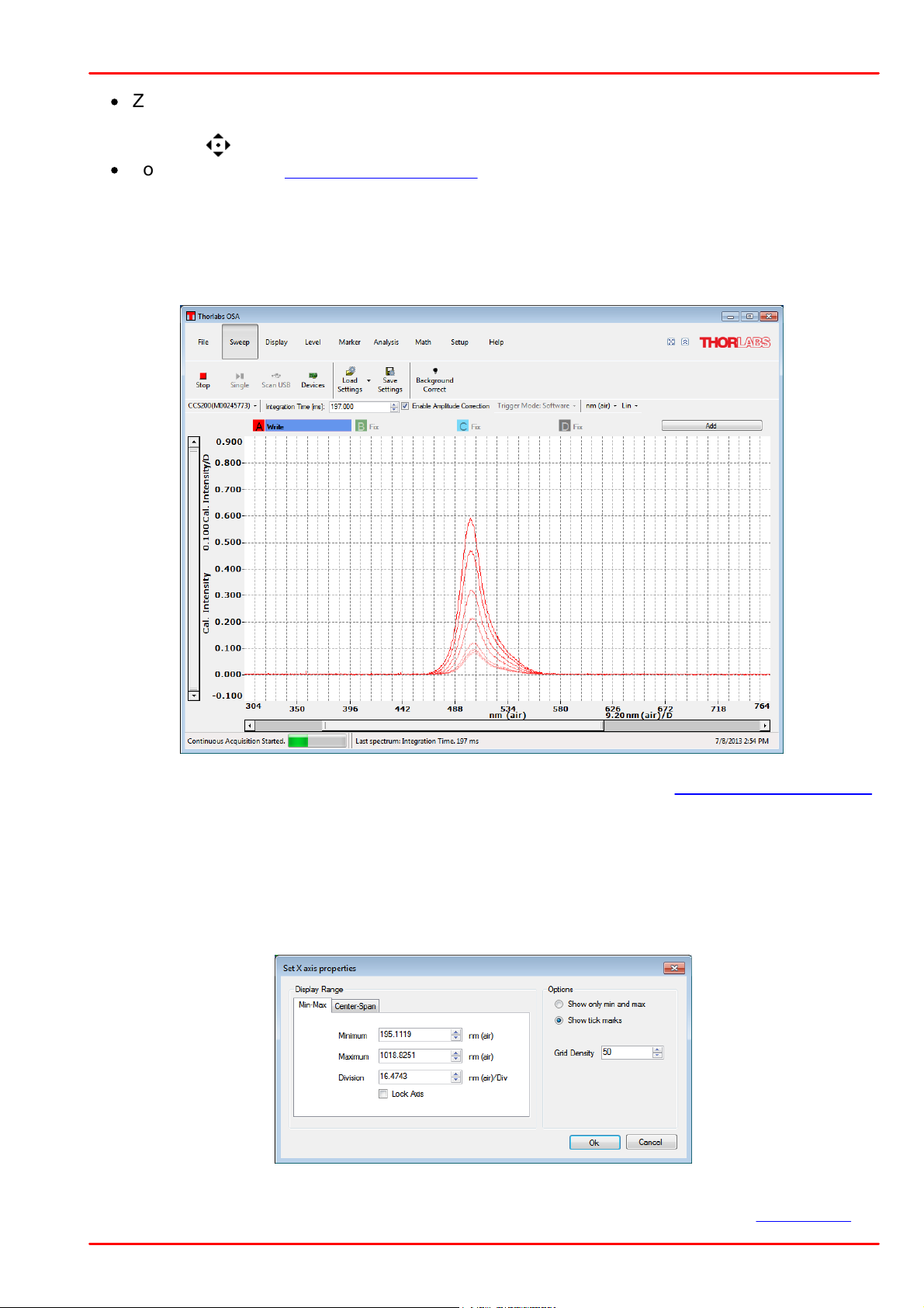
Persistence

Enabling persistence in repeat sweep mode, a finished scan won't be overwritten with the next spectrum acquisition, but it will remain decreasing in brightness:

The persistence speed, i.e. how fast previous scans cease, can be set in Setup menu, tab Display.

X Axis Properties Dialog

The settings of the wavelength axis can be set in an extended way. Left click to the numbers' area of the wavelength axis and the "Set X Axis Properties" dialog

comes up. It has two tabs - one for setting the axis' minimum and maximum, the 2nd to set the center wavelength and the wavelength span.

Display range: Here can be entered two values, the 3rd value is being calculated from the two entered and the grid density. The units are corresponding to the choice made in the settings bar.

CCS Series Spectrometer

In the Center - Span tab the central wavelength and the entire span can be defined. Common controls:

Lock axis: When this box is checked, the wavelength range cannot be zoomed using the scroll wheel, only numerical entries are accepted.

Options: Here the selection can be made to display only min and max wavelength or min, max and intermediate wavelength numbers.

Grid density: Select, how many grid are distributed over the wavelength display range.

4 Operating Instruction

4.1.4 Level

In the Level menu the intensity axis display can be configured. From the drop down menu a quick selection of the display preferences can be made - either set the min and max intensity, or set a min intensity and the display division. Further, if level markers are enabled (markers 3 and 4), the display can be zoomed in on the range between the 2 markers ("Get from Level Markers").

Y Axis Properties Dialog

The settings of the intensity axis can be set in detail. Left click to the numbers' area of the intensity axis. The "Set Primary Y Axis Properties" dialog

comes up. It has two tabs - one for setting the axis' minimum and maximum and another to set the center wavelength and the wavelength span.

Display range: Two values can be entered here. The 3rd value is calculated from the grid density and the two entered values. The units are intensity or calibrated intensity values (if amplitude correction is disabled or enabled, accordingly).

In the Center - Span tab, the central intensity and a span around this central intensity can be defined.

Common controls:

Lock axis: When this box is checked, the intensity auto zoom function (right click into the display area) is disabled; only numerical entries are accepted.

Options: Here the selection can be made to display only min. and max. intensities or min., max. and intermediate intensity values.

Grid density: Select how many grids are distributed over the intensity display range.

CCS Series Spectrometer

Movable Markers

4.1.5 Marker

The OSA software offers two types of markers - movable and fixed.

4.1.5.1 Movable Markers

Movable Markers

The movable markers can be used to inspect the value of the data at different positions, to change the displayed area of the graph (see zooming the

vertical axis and zooming the horizontal axis), or

to place fixed markers. There are four movable markers: two line

markers - Markers 1 and 2 - and two level markers - Markers 3 and 4. Enable and disable them by pressing the respective buttons in the “Marker” menu. The markers can also be enabled and disabled by pressing Ctrl and their respective number on the keyboard.

As soon as at least one movable marker is enabled, the marker panel appears to the right of the spectrum display. It contains detailed information:

for line markers: wavelength and corresponding intensity value of the active trace for each marker and (selectable) the difference or quotient of their wavelengths

for level markers: intensity value level and

(selectable) the difference or quotient of their intensity levels on the primary axis.

difference / quotient are displayed only if both appropriate markers are enabled.

Moving

Place the mouse cursor over the marker, the mouse pointer changes to . Press and hold the left mouse button down to drag the movable marker to the desired position.The position of the movable markers can also be changed by clicking on the number of a marker to move in the cursor panel. This brings up a dialog to set the position of the marker numerically:

For the actual marker, either it's absolute position or it's position relative to the the paired marker can be entered numerically.

4 Operating Instruction

Marker Options

Clicking to Marker Options, some additional marker features can be configured:

Both the line and level markers can be locked / unlocked. When locking a marker pair, their distance will remain constant when moving one of them. By clicking the pad lock icon, the lock status can be toggled.

The relation between the 2 markers can be displayed as their quotient (ratio) or difference.

"Decimals Displayed" allows to select 1 to 11 decimals or "auto".

Automated Peak Search functions The Peak Search and Search Left (Right) buttons allow to quickly set line marker #1 to a peak.

Note : Prior to using this button, the peak search criteria, such as search wavelength range,

threshold and minimum peak height, must be set in the menu Setup -> Peak Track! Press Peak Search to find the highest peak within the selected wavelength range. When pressing

Peak Search repeatedly, the line marker #1 will jump to the next lower peak, after finding the last peak, it jumps back to highest. Search Left and Search Right buttons move the cursor to the next adjacent peak in the stated direction.

For each peak position, the wavelength and correlated intensity will be shown numerically as shown in the figure Movable Markers.

CCS Series Spectrometer

4.1.5.2 Fixed Markers

The Thorlabs OSA software can handle up to 2048 fixed markers. A fixed marker has a fixed position, is connected to a single trace (not necessarily the active trace) and will track the intensity value at the given wavelength. The fixed markers are identified by a number, starting with 0 for the first fixed marker added. The levels of the fixed markers can be tracked in a time series analysis.

Each fixed marker added is shown in the spectrum display as a triangle with its identifying number above it. The location of the triangle is determined by the position of the fixed marker and the value of the connected trace at the given position.

The values of the fixed markers and their positions can be stored to file or copied to clip board for processing in other software.

Adding

In the currently active trace, a fixed marker can be derived from line marker 1 - just press the button “Add Fixed”. The fixed marker is added to the trace, and below the trace a table comes up with detailed numerical characteristics of the fixed markers:

Table Columns:

Marker number - the number displayed in the diagram above the appropriate fixed marker. The first marker (number 0) is the reference marker.

Trace - the correlated trace character is displayed (not necessarily the active trace!)

Position - X axis position, at which the marker is located. The header states the unit, as set up in the settings bar.

Level - the level of the trace at the marker's position. The header shows the unit, depending on the current trace function.

Δ Position - the distance to the position of the previous marker, in the same unit as column Position

Offset - the distance to the reference marker (# 0), in the same unit as column Position.

Δ Level - level difference between the actual and the reference marker, in the same unit as column Level

4 Operating Instruction

Remove Fixed

Any fixed marker can be removed individually by moving line marker 1 to the position of the fixed marker and pressing the button “Remove Fixed”. Alternatively, right click in the table to the line of the fixed marker that shall be removed and select "Remove Marker" from the table options.

Clear Fixed

This button removes all fixed markers from the trace.

Mark Peaks

Pressing the button “Mark Peaks” will add one fixed marker to each automatically detected peak that corresponds to the peak finding settings in the currently active trace. The first marker will be added to the highest peak in the spectrum, the second marker to the second highest peak, etc.

Note: This will add fixed markers to the found peaks in the currently active spectrum; the positions

of these markers will not change until they are removed.

Table Options Menues

The menu "Save Table to File" opens a dialog to store the fixed marker table in CSV format. This can be done also by right clicking to the table and selecting “Save Table to File”.

A previously saved table can be opened using the "Load Table from File" button.

The very right button copies the table to the clipboard, this way the table can

be quickly pasted to other software (e.g. EXCEL). This can be done also by right clicking to the table and selecting "Copy Table".

The columns of the table to be displayed can be selected from the Select

Columns button:

Quick access to marker table

Click to a marker table element, the marked line will be highlighted and an ► appears to the left of the marked line. Right click to the table and an options menu comes up:

Set As First Marker moves the marked line up to position #0, this

way making this marker to reference.

Remove Marker deletes the current marker from the list and from

the display.

Order by intensity rearranges the table by increasing / decreasing intensity

Order by Position rearranges the table by the markers' positions on the X axis (increasing / decreasing)

Copy Table copies the entire table to the clipboard

Save Table To File opens a dialog to store the table in CSV format

Increase (Decrease) font size can be used to improve the visibility of the table's content.

CCS Series Spectrometer

4.1.6 Analysis

Note

The grayed-out features are available only for if the active device is an OSA20x spectrometer. Color Analysis button is shown only with amplitude correction enabled.

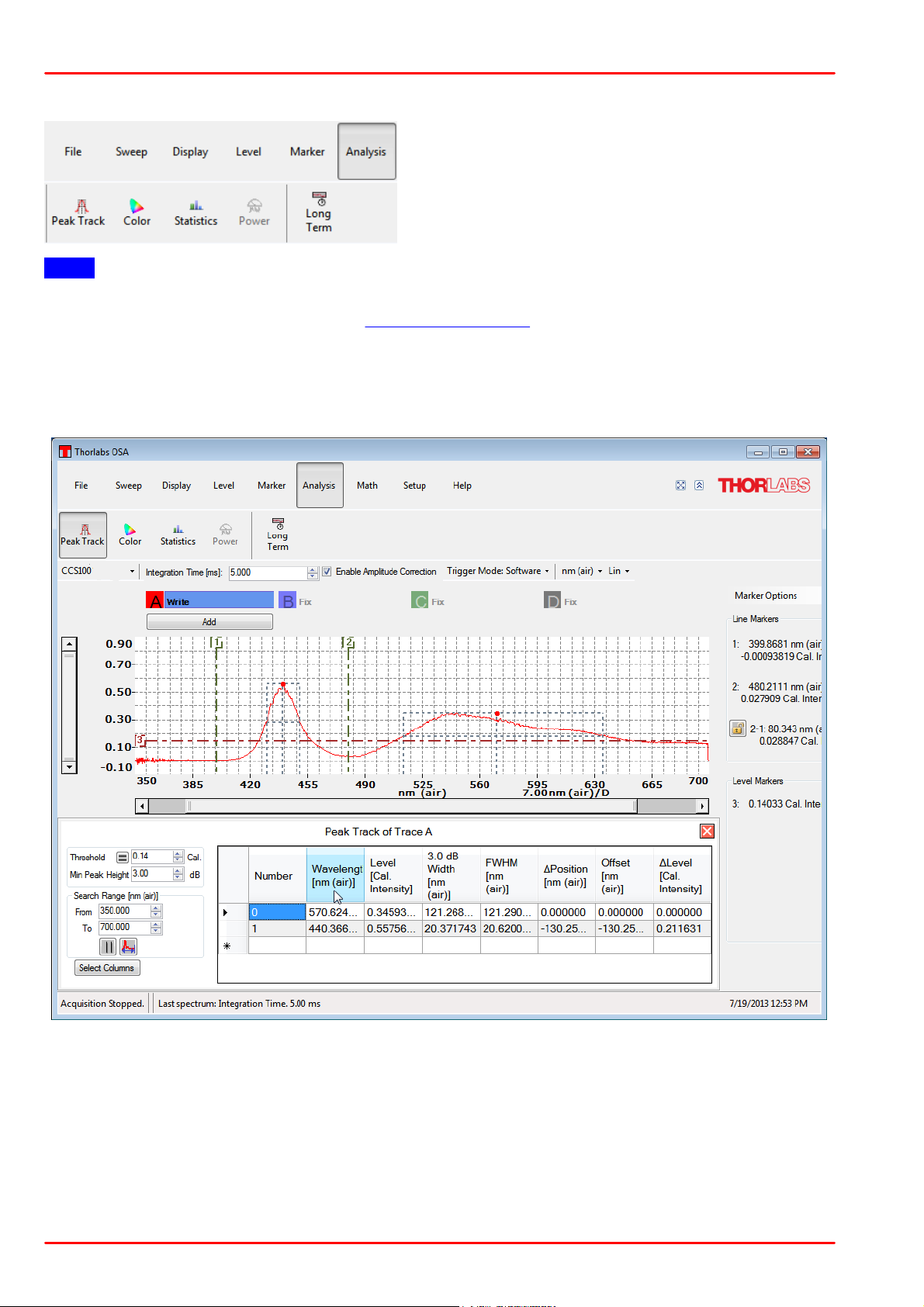
4.1.6.1 Peak Track Analysis

In Peak Track analysis mode, the position, amplitude, and width of peaks in the spectrum can be tracked over time.

As long as the Track Peak mode is active, the Track Peak analysis area will be displayed below the data display. Here, a data table shows information about the peaks and as well as a small toolbox with the settings that used to find the peaks. It is also possible to select which columns can be displayed in the data table by clicking on the button “Select Columns”.

4 Operating Instruction

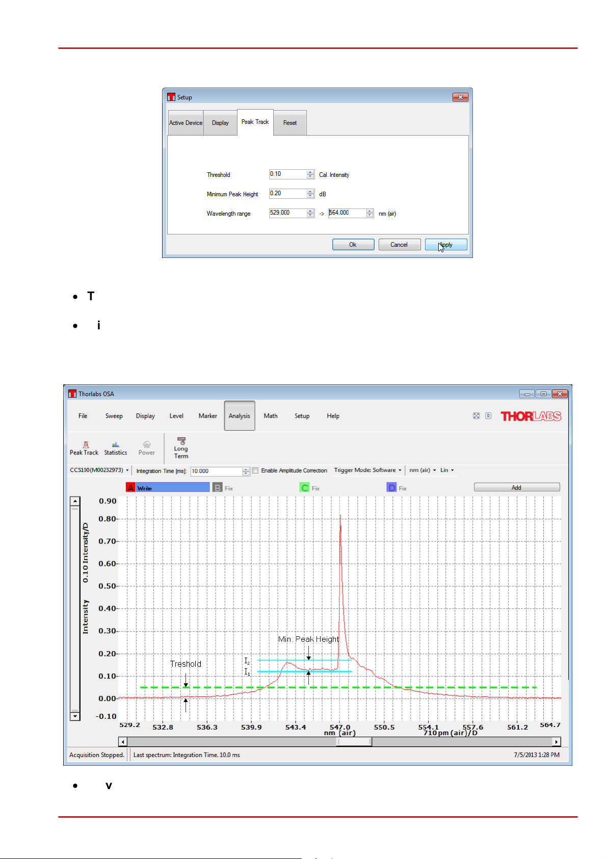
The parameters used to find the peaks are:

Threshold: Only data points with intensity above this level will be used when searching for peaks. Threshold can be entered manually or retrieved from a level marker (click to )

Min Peak Height: Only peaks that have a peak-to-base ratio of at least this value will be found.

Note The Minimum Peak Height affects the reported width of the peaks - it's the width of the

peak at this level from the maximum value. For example, a value of 3 dB here will give the FWHM of the peak and a value of 6 dB here will give the width of the peak and a quarter of the maximum value.

Search Range: (Wavelength / Wave number / Frequency): Limits the x-axis range in which the search for peaks is performed. It can be entered numerically, retrieved from line markers (

) or from the currently displayed range ( ).

In Track Peak mode, the currently active spectrum is checked for peaks upon the collection of a new spectrum from the instrument. The peaks are by default sorted in order of decreasing intensity. The sorting can be changed by left clicking to the parameter. In above screenshot the peaks can be sorted by increasing / decreasing wavelength (toggling).

Right clicking in the data table brings up a dialog to:

add a fixed marker at the highlighted peak;

Move movable markers to this peak:

Line marker 1 will be set to the peak wavelength Line marker 2 displaced from peak wavelength for + half the FWHM Level marker 3 to the peak level Level marker 4 to the FWHM level

increase / decrease font size in the table

copy the table - it can be pasted then directly to other applications like Microsoft EXCEL

save the table to file (CSV file with selectable separator)

The peaks found in Track Peak mode can be tracked over time in a time series analysis (see the Long Term Tests) if the Track Peak analysis mode is started before the time series analysis is

CCS Series Spectrometer

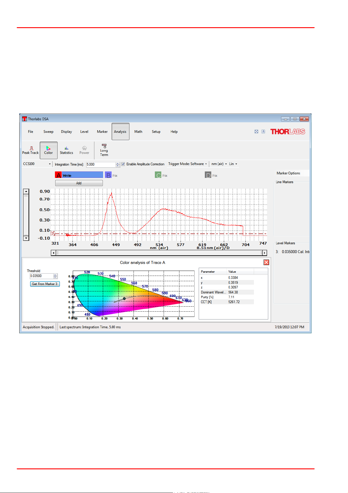
Color Analysis of a Thorlabs MCWHL4 cold-white LED

started. Notice that since the peaks are ordered by decreasing intensity, they can be rearranged if the relative intensity of the peaks in the spectrum is changed.

If no peaks are found in the Track Peak mode, check the settings for the threshold and min-peak height to make sure that the expected peaks in the spectrum are higher than this. The settings can be changed either in the Setup Dialog or directly in the Options Control box found to the right of the data table in the Peak Track Analysis area.

4.1.6.2 Color Analysis

The Color Analysis performs a color analysis of the currently active trace. The analysis calculates the chromaticity coordinates (x, y, and z) and the main wavelength in the spectrum.

The Thorlabs OSA software calculates the correlation between the collected spectrum and the three color matching functions x(λ), y(λ), and z(λ) defined from the CIE 1931 2° standard observer to obtain the tri-stimulus values X, Y, and Z. These are then normalized to obtain the chromaticity coordinates x, y, and z.

The calculated chromaticity coordinates x and y are displayed in the CIE 1931 color space chromaticity diagram as a dark circle as well as displayed numerically next to the diagram.

The dominant wavelength is calculated as the interception between the straight line from the white point (1/3, 1/3) through the calculated chromaticity point (x, y) and the edge of the chromaticity diagram.

4 Operating Instruction

The purity is calculated as the portion of the distance from the white point (1/3, 1/3) to the edge of the chromaticity diagram that the distance from the white point (1/3, 1/3) to the calculated chromaticity represents. A purity of 100% represents a point on the edge of the chromaticity diagram, i.e. a pure color, and a purity of 0% represents a mix of all colors, i.e. the white point itself.

The Correlated Color Temperature (CCT) can be calculated for a light source that is close enough to the Planckian locus in the 1960 UCS. The CCT is calculated by converting the calculated chromaticity point (x, y) into a point in the CIE 1960 color space (u, v) and finding the closest Planckian locus. If the distance to the closest Planckian locus (Δu,v) is larger than 0.05 then a temperature of -1 Kelvin is returned as an error code.

The threshold option makes it possible to ignore data points in the spectrum with low intensity; this can be useful e.g. if the spectrum is very noisy. For easy handling, the threshold can be defined by a level marker.

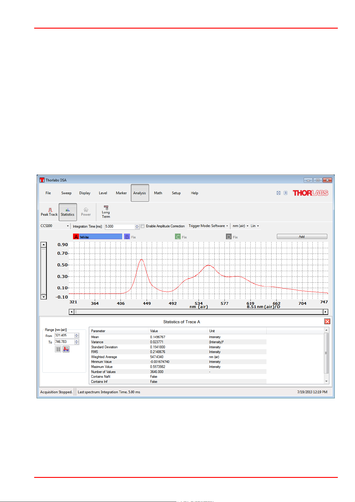
4.1.6.3 Statistics

The Statistics function displays statistical values of the acquired spectral intensities over the specified wavelength range.

CCS Series Spectrometer

4.1.6.4 Long Term Analysis

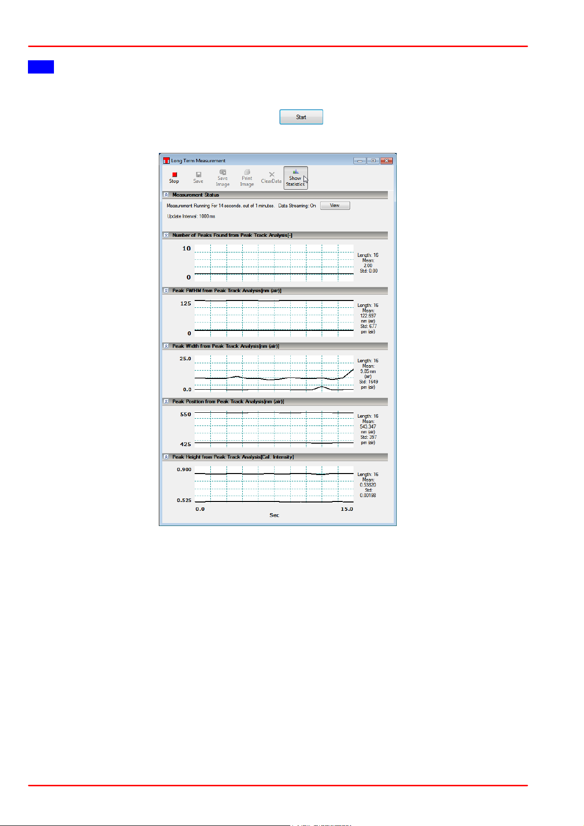
Long Term Analysis allows to record selectable spectral data over a selectable period of time.

Note

Make sure that prior to starting the Long Term Analysis the OSA software executes repeated sweeps, otherwise the active trace won't be updated!

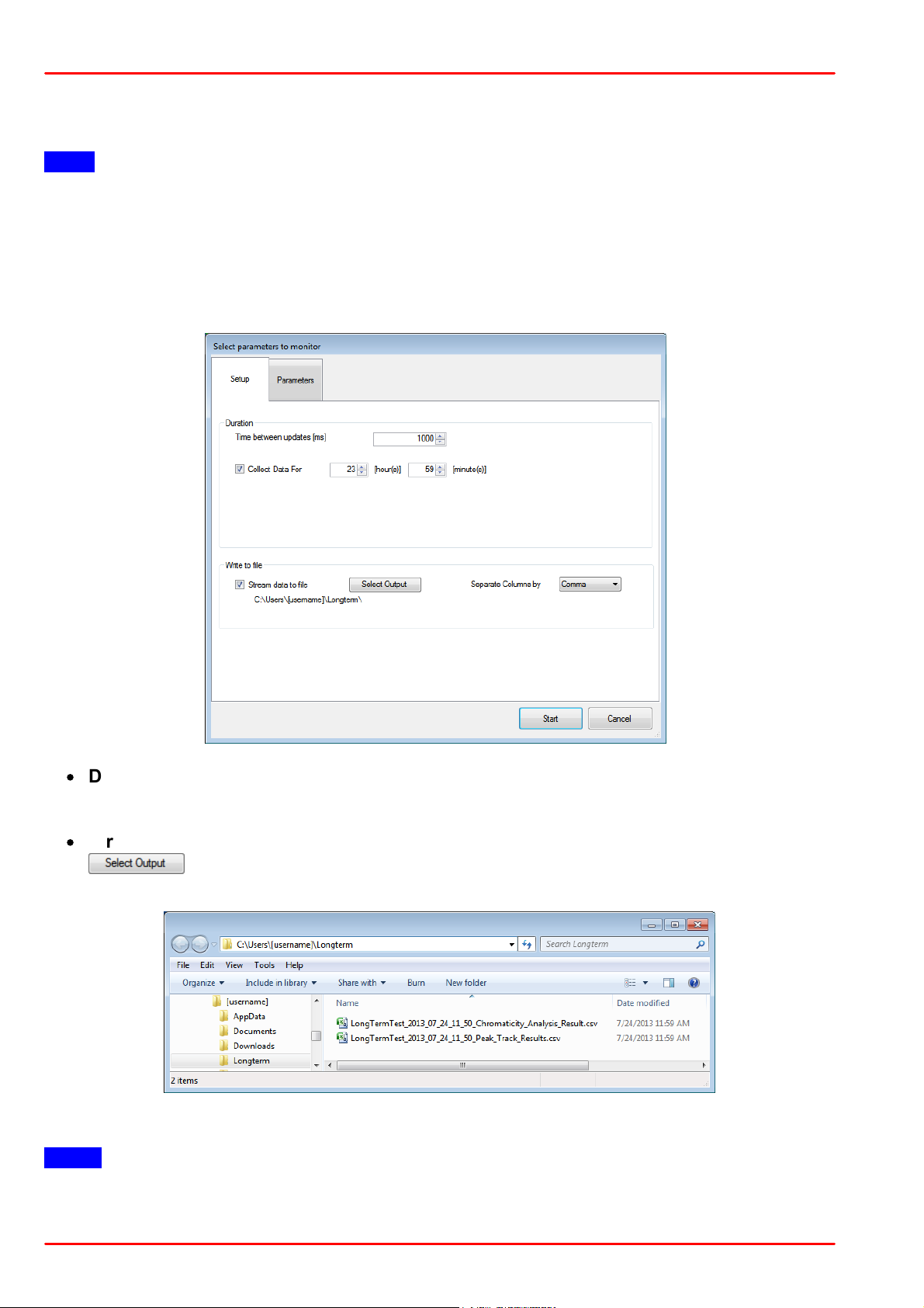
Click the button "Long Term" to enter the dialog on duration, output file and parameters to be observed.

Tab Setup

Duration: Select the time between two updates, the possible interval is 1 ms to 1,048.576 s. "0 ms" disables update. The data collection can be limited - check the box "Collect Data for" and enter the desired analysis time

Write to file: The collected data are streamed to a CSV file. Select the output folder (

) and the separator. The data will be saved to individual for each parameter files,

for example:

Tab Parameters

Note: Only parameters from the active trace can be logged!

In order to enable a parameter to be logged, check the box "Active trace". For each parameter some additional settings can be made.

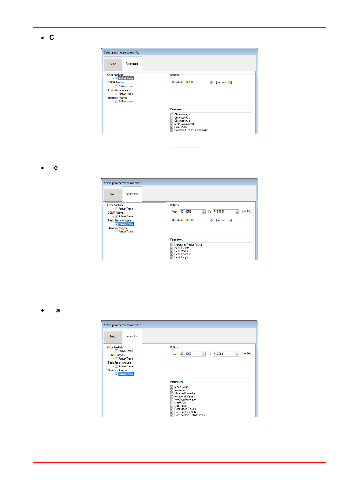
Color Analysis:

Options: Enter the desired intensity threshold Parameters: Select the Color Analysis parameters that should be logged.

Peak Track Analysis:

4 Operating Instruction

Options: Select the wavelength range. By default, the entire operating wavelength range

of the recognized CCS spectrometer is stated. Select the desired intensity threshold.

Parameters: Select the Peak Track Analysis parameters to be logged

Statistics Analysis:

Options: Select the wavelength range. By default, the entire operating wavelength range

of the recognized CCS spectrometer is stated.

Parameters: Select the Statistics parameters to be logged.

CCS Series Spectrometer

Note

The more parameters are logged, the higher the CPU load caused by Long Term Analysis. This can lead to delays in graphic display updates and reaction time to controls of the OSA software!

After all selections were made, start the logging ( ). The Long Term Measurement window opens showing the progress:

Stop (Continue) The current data collection can be interrupted and continued. Save Saves the measurement results as a CSV file Save Image Saves the measurement results as an image. Available formats: PNG,

JPG, BMP

Print Image Prints the measurement results to any installed printer. Clear Data Deletes the collected in the display data Show Statistics Current statistic values for each parameter can be displayed by clicking to

the appropriate button in the header:

- Length: Expired time

- Mean value

- Standard deviation of the mean value

4 Operating Instruction

4.1.7 Math

The buttons on the math menu all work on the currently active trace and are disabled while collecting spectra. The math operations can be undone by pressing the “Undo” button.

Spectrum Math

This brings up a dialog making it possible to perform mathematical operations on one or several spectra, e.g. multiplying a spectrum with a scalar, adding together two spectra or dividing one spectrum by another. The expression to be calculated is typed into the text box of the dialog that is opened with the following rules for formatting

Traces are identified by capital letters A through Z. Only the traces which can be seen in the trace controls area can be used.

Scalars with decimal fractions are entered using a decimal point to separate the integers from the decimals.

Allowed operators are, + (indicating addition), - (indicating subtraction), * (multiplication) and / (division).

Operations can be grouped using round parentheses.

The calculation will be performed when the button ‘Calculate’ is pressed. Pressing the button ‘Close’ will close the window without doing anything more.

Cut Spectrum

This function is available only if the two movable line markers are enabled and will cut the currently active trace to the region between the two line markers, removing all data outside the selected range.

Invert

Calculates and displays the reciprocal of the currently active trace.

CCS Series Spectrometer

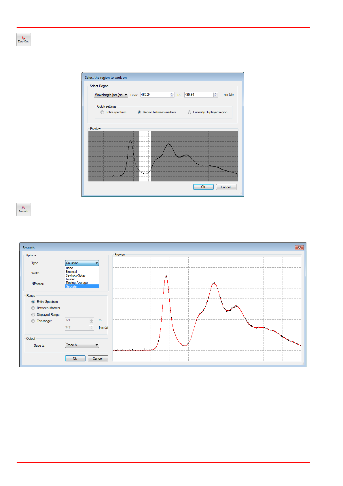
Zero Out

Sets all values between in a specified region of the spectrum/interferogram to zero. This brings up a dialog where the region can be specified.

Smooth

Performs a smoothing operation on the currently active trace and brings out a dialog in which it is possible to select a smoothing algorithm to use and to set the parameters for the smoothing.

The trace to operate on is displayed in black in this dialog and the smoothed spectrum is displayed in red. Beside the displayed by default Gaussian smoothing, there are available a number of alternative smoothing methods.

Further, the wavelength range to be smoothed and the output trace for the smoothed spectrum can be selected

4 Operating Instruction

Curve Fit

This function allows to fit a mathematical curve to the currently active trace or a portion of it.

In the "Curve Fit Dialog" you can select:

The mathematical fit function (Gaussian, Lorentzian and Polynomial)

The data range to be used for fitting:

- Entire trace: Every data point in the currently active trace will be used to fit the function.

- Trace Between Markers: (only available if both Line Marker 1 and 2 are shown). Every

data point between the two line markers will be used in the fit.

- Displayed Range of Trace: Every data point which is currently visible in the main window data display will be used in the fit (NOTE: this is not the region currently displayed in the curve fit dialog).

- Fixed Markers: (only available if at least one fixed marker is shown). Only the data points at the currently set fixed markers will be used in the fit. Use this option to e.g. fit a curve to a set of peaks in the spectrum.

- This Range: Makes it possible to specify a given x-axis range that will be used in the fit.

The output trace where the fit result shall be stored.

Pressing the ‘Ok’ button will start the fit. If the fit failed then the status bar will display the error message ‘Fit Failed’.

Note

The fitted function will be applied only for the x-axis (data) range that was used to create the function.

CCS Series Spectrometer

Derivative

Calculates the derivative of the current trace. Derivatives are available up to the fifth order.

Add Noise

White noise with a selectable SNR can be added to the spectrum.

Convert Unit

Calculator to convert units used by the software each into the other.

Resample Data

Change the sample points in the current trace. Brings up a dialog to select the resampling factor. The resampling factor is the desired length of the trace divided by the current length of the trace.

Example:

- Selecting a resampling factor of 0.5 reduces the length of the trace by a factor of two

- A resampling factor of 4.0 increases the length of the trace by a factor of four.

The resampling is performed using a quintic spline interpolation to make the resampled trace as similar to the original trace as possible.

4 Operating Instruction

Input traces (A and B)

Output trace C

Option - "Keep Original Data Points"

Output trace C

Option - "Average Traces"

Stitch Traces

Two traces, originated from different spectrum acquisitions, can be stitched. The settings dialog

lets you select the data sources (input traces), the output trace and the option for overlapping. To illustrate that, please see the following screen shots:

CCS Series Spectrometer

Synthetic Spectrum

A synthetic Black Body Spectrum can be created with a number of individual settings.

4.1.8 Setup

Click to Setup button in main menu. A dialog window with 4 tabs comes up:

Active Device

Display

Peak Track

Reset

4.1.8.1 Tab Active Device

4 Operating Instruction

The active device tab shows information on the active instrument and has 3 sub-tabs. Common: Set integration time and trigger mode. The integration time can be set between 10µs

and 60 s. The trigger source can be internal (software trigger) or external via the SMB connector.

Amplitude correction:

Note

The amplitude correction will work properly only if the CCS spectrometer was factory calibrated for amplitude correction!

The factory amplitude correction can be carried out only for wavelengths > 380 nm. With enabled amplitude correction, the intensity is displayed "calibrated", i.e., taking into account

the wavelength dependent responsivity of the CCS spectrometer. This leads to an increase of the noise at wavelengths with lower responsivity, as not only the wanted signal is amplified, but also the noise. In the setup panels this increase of noise is stated as "Noise amplification", which is in fact the ratio of the max. and min. responsivity (in dB) within the given wavelength range. The amplitude correction can be configured in two setup modes: Wavelength Range (recommended for accurate intensity results in a give wavelength range) and Noise amplification (recommended if weak intensities are measured and a minimum noise interference is required). The two examples below explain both modes in detail.

CCS Series Spectrometer

Spectrum with Amplitude Correction disabled

Spectrum with Amplitude Correction enabled

Example 1: A spectrum of a cold-white LED shall be displayed with calibrated intensities between 470 and 660 nm.

Open in the Setup Menu the tab "Active Device" and then the sub-tab "Amplitude correction", select Setup Mode "Wavelength Range":

Enter the desired wavelength range; the OSA software calculates the "Noise amplification" and displays it. The screenshots below illustrate how enabling the amplitude correction affects the spectrum display of a.m. cold white LED with above settings. For better visualization, line markers are inserted at the lower and upper limit of the corrected wavelength range:

4 Operating Instruction

Spectrum with Amplitude Correction disabled

Spectrum with Amplitude Correction enabled

Example 2: A spectrum of the same cold-white LED shall be displayed with calibrated intensities around the peak wavelength of 400 nm with a max. noise increase of 1.6 dB:

Open in the Setup Menu the tab "Active Device" and then the sub-tab "Amplitude correction", select Setup Mode "Noise Amplification":

Enter the desired center wavelength and the allowed noise amplification; the OSA software calculates the resulting min. and max. wavelengths. The screenshots below illustrate how enabling the amplitude correction affects the spectrum display of a.m. cold white LED with above settings. For better visualization, a line marker is inserted at the center wavelength range:

CCS Series Spectrometer

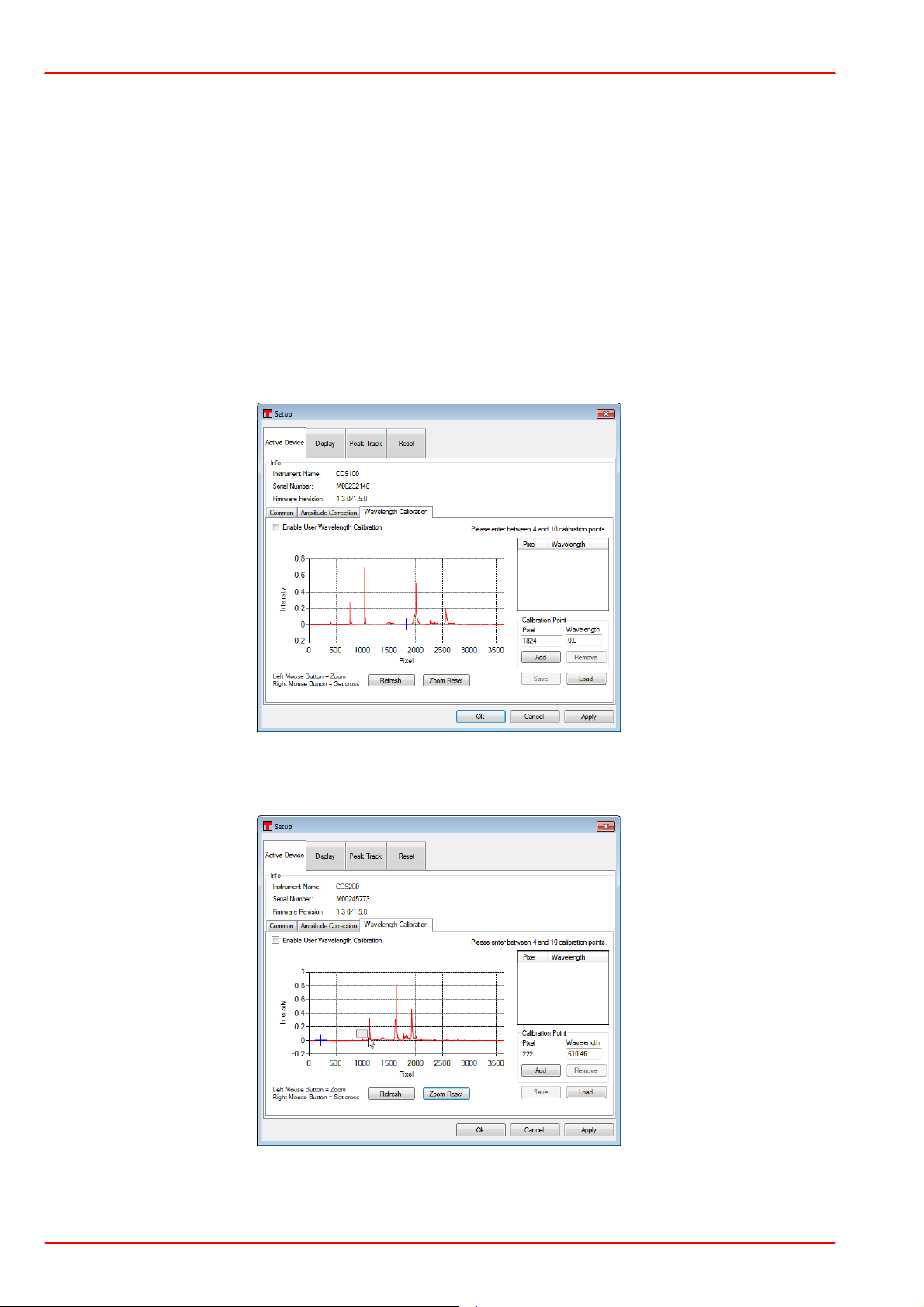
Wavelength Calibration

The sensor of a CCS spectrometer is CCD line. Depending on the wavelength, the incident to the spectrometer light is directed to a certain pixel of the CCD line. Each CCS spectrometer is factory calibrated, using a calibration source with well-known spectral lines. The factory calibration is saved to the internal non-volatile memory and defines the exact wavelength for a number of pixels. Between these calibration points, the wavelength is interpolated.

In certain cases a more detailed user calibration, based on an available calibrated spectral source, might be desired. The user can then replace the factory calibration with a user calibration, consisting of a min. of 4 and a max. of 10 individual calibration points.

First of all, apply the individual spectral source to the CCS spectrometer input and adjust the integration time in such way that maximum intensities are displayed without entering saturation.

Then Setup -> tab Active Device -> subtab Wavelength Calibration:

The small display can be easily zoomed by dragging the desired zoom area with left mouse button hold pressed.

When release the left mouse button, the display appears zoomed. Move the mouse to the peak and press right mouse button. The peak will be marked now by a blue cross and the related pixel number will be displayed in the Calibration Point box:

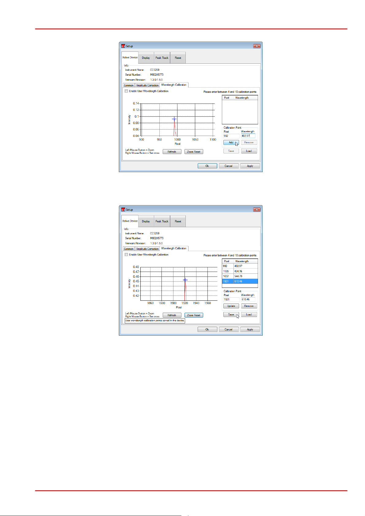
4 Operating Instruction

Enter the corresponding wavelength and press Add button - the calibration point will be added to the table. Repeat these operations until at least 4 calibrations points are entered.

Any calibration point in the table can be edited by following the steps below:

- mark it in the table

- the data will appear in the input box.

- correct the wavelength

- press Update - the table will be updated.

After the calibration table is complete, press Save. The user calibration points will be stored to the CCS spectrometer. From now on, the wavelength calibration can be switched between Factory and User Calibration by checking the box "Enable User Wavelength Calibration"

CCS Series Spectrometer

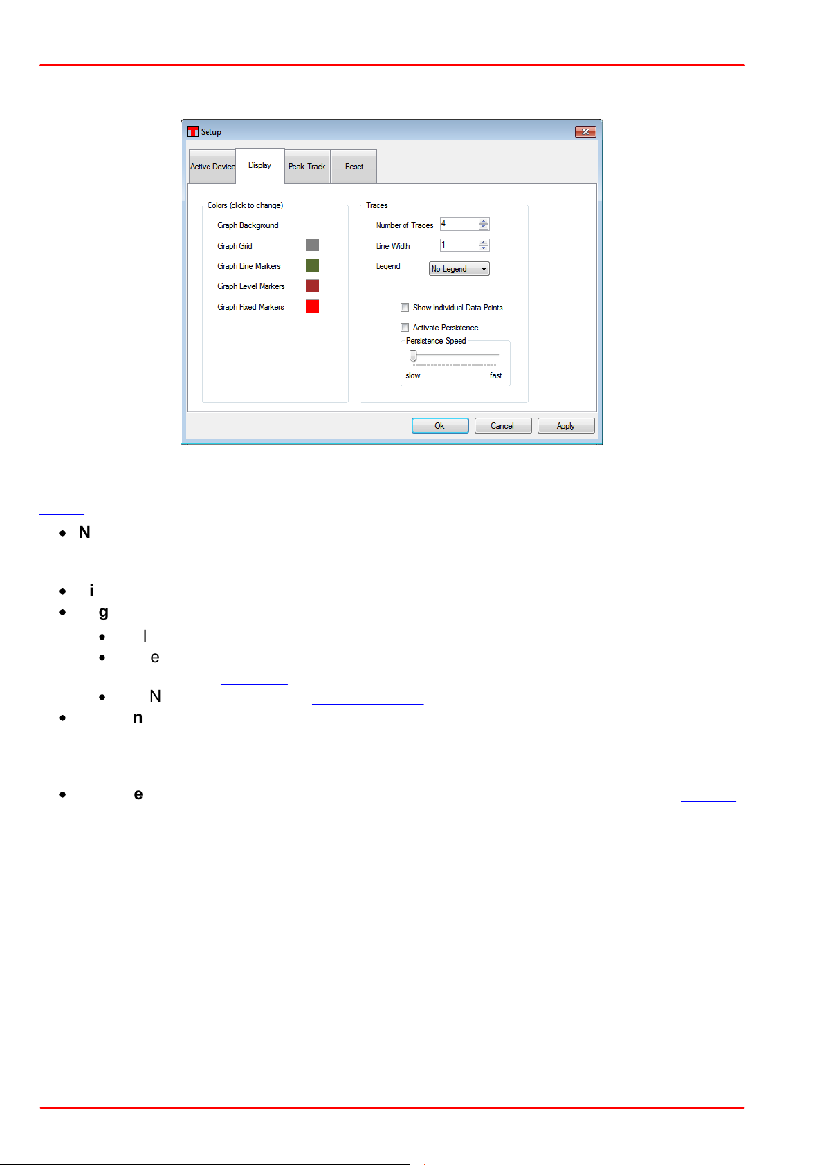
4.1.8.2 Tab Display

The left part is dedicated to the color setup of the graphic elements in the spectrum display. Click to a color to open the Windows color setup dialog. In the right part, the common settings of the

traces can be configured:

Number of traces defines the default number of traces, that are displayed with OSA software start. Traces can be added during a software session, but with a software restart, it returns to this default.

Line width of the spectrum can be set between 1 and 10.

Legend is a drop down menu to select the content of the legend displayed with each trace:

No legend

Trace Name; Trace Comment: The legend box displays the appropriate information, entered to the trace info.

File Name: If the trace was loaded from file, the appropriate file name is displayed.

Show individual data points displays all data points (X;Y) as a "+". Each CCD pixel generates a single data point, so the individual data points can be seen only if sufficiently zoom in the X axis. For example, the distance between two adjacent data points of a CCS100 is abt. 110 pm.

Persistence Speed adjusts the ceasing speed of previous scans. See also section Display.

4 Operating Instruction

4.1.8.3 Tab Peak Track

Set in the Peak Track tab the criteria for detecting a peak:

Threshold is the minimum intensity of a track given in absolute intensity (calibrated intensity) value.

Minimum Peak Height is the min ratio in dB of a detectable peak intensity (I2) to the surrounding baseline intensity (I1). These two parameters are illustrated below:

Wavelength Range limits the peak finding range.

CCS Series Spectrometer

4.1.8.4 Tab Reset

The button "Restore Factory Defaults" in the Reset tab returns the GUI to an initial state. The factory default settings of the GUI are:

X axis units: nm (air)

Y axis units: Intensity

Y axis display: linear

Int. time: 1.0 ms

Amplitude Correction set to "Wavelength Range", not enabled

Trigger mode: Software

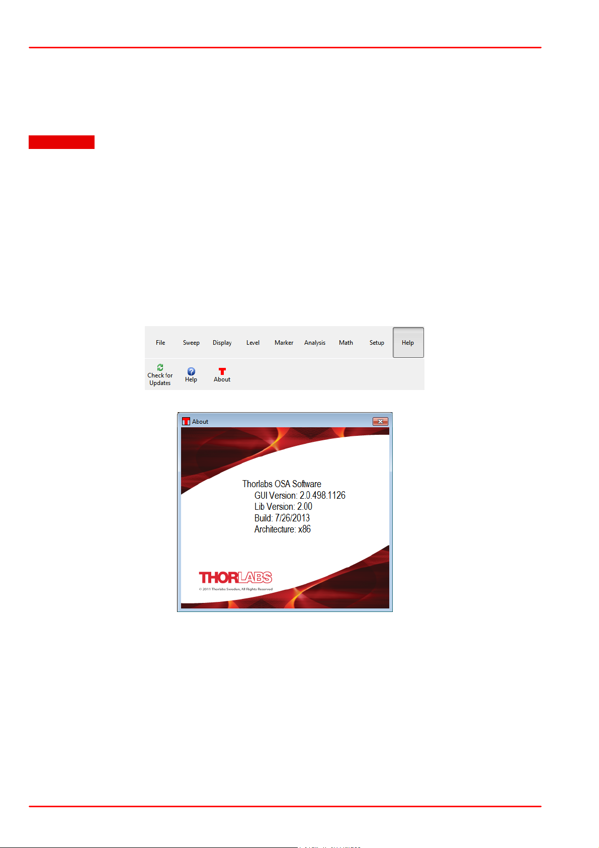
4.1.9 Help

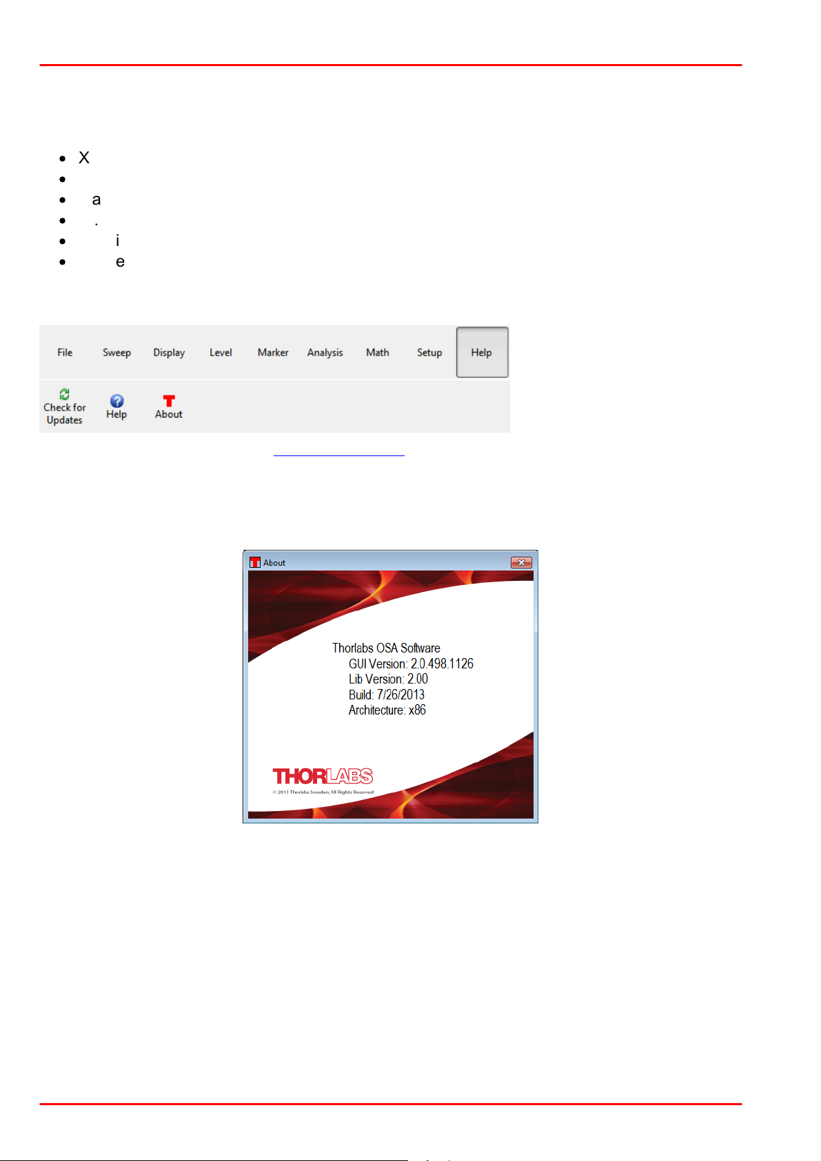
Check for updates connects to www.thorlabs.com and verifies if a software update is available. Help opens the OSA software online help. About displays detailed information about the OSA Software. Please have these details available

when contacting our Tech Support with technical questions:

4 Operating Instruction

4.2 Settings Bar

Via the settings bar, some important parameters can be accessed quickly and independently of the currently used main menu item:

Switch Instrument

This drop-down menu allows you to quickly switch between connected and recognized spectrometers.

Note After switching to a different instrument, at least a single spectrum acquisition is necessary

to update the spectrum display axes.

Set Integration Time

Change integration time by entering numerical values, scrolling the mouse wheel or using up-down arrows.

Enable / disable Amplitude Correction

With enabled amplitude correction, the intensity is displayed "calibrated", i.e., taking into account the wavelength dependent responsivity of the CCS spectrometer. The amplitude correction can be optimized for a wavelength range of interest or for a certain required SNR (signal-to-noise ratio). For details please see in section Setup.

Note This will work properly only if the CCS spectrometer was factory calibrated for amplitude

correction! The factory amplitude correction can be carried out only for wavelengths > 380 nm.

Switch Trigger Mode

The trigger mode can be selected between internal ("Software") and external via the SMB

connector.

Switch X Axis Units

The X axis can be displayed using different units:

wave number [cm-1]

wavelength in air [nm (air)]

wavelength in vacuum [nm (vac)]

frequency [THz]

photon energy [eV]

For detailed information, please see the tutorial.

Switch between linear and logarithmic Y axis

Switch the Y axis scaling between linear and logarithmic.

CCS Series Spectrometer

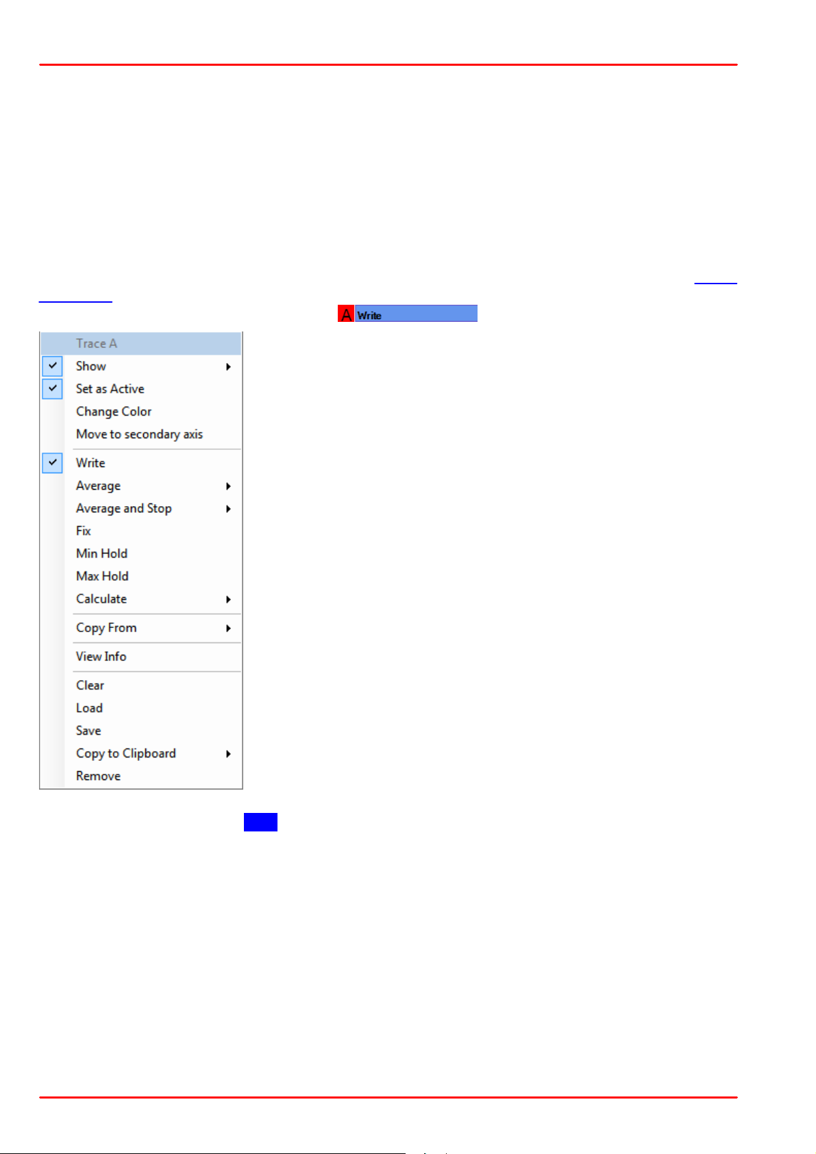
4.3 Trace Controls

The acquired spectra are displayed in “traces.” The Thorlabs OSA software can handle up to 26 traces labeled from “A” to “Z”; the most left trace is always A followed by B, etc. The controls for the traces are located below the settings bar. The color of each trace is shown as background of the trace letter; traces which are not displayed in the data display area are shown in a faded out color. To the right of the trace letter (“A”, “B”, etc.) the update option for the trace is displayed, determining what will happen with the trace during the next data acquisition.

Additionally, a legend can be displayed showing for all not hidden traces their color and a selectable text. The legend can be placed to any location within the spectrum display. The initial trace settings (number of traces and their appearance) at program start are configured in the Setup

-> Display menu. After program start, trace A is set as active and will be updated with each new

data acquisition. Click to the trace header to open the Trace properties menu:

Show Toggle to show / hide the trace. Additionally, all other traces can be shown or hidden at one click. The trace header remains when a trace is hidden.

Set as Active Setting a trace active enables further operations (saving, loading, etc.).

Change Color Change the trace color

Move to Secondary Axis By default, all traces have a common Y

axis. This may become inconvenient, particularly, if one trace displays e.g. intensity (max =1.0), and another trace a ratio that may reach thousands of units. In such case, the software automatically zooms the Y axis to the trace with the widest range, as a consequence the intensity trace becomes almost a flat line. In such case, a trace can be moved to secondary axis, that appears to the right of the spectrum display area. The primary and the secondary Y axes can be zoomed independently.

Write Set a trace to Write in order to update it with the next acquired spectrum.

Average / Average and Stop The number of acquisitions to be average can be set. The averaging method is rolling average (over the last "n" acquisitions). There are several presets from 5 to 200 averages, other values can be entered by pressing the Custom

button. The "Average and Stop" terminates the spectrum display update after finishing the given number of averages. Please note that the spectrum acquisition however continues. To display recent acquisitions, uncheck the "Average and Stop" option.

Fix Fixes the content of the current trace, i.e., it will not be overwritten with next acquisition.

Min (Max) Hold If the spectrum intensity changes with a new data acquisition, this function holds

the minimum (maximum) intensity value.

4 Operating Instruction

Calculate The calculation capabilities depend on the trace letter. Trace A: Only user defined calculations are possible

Trace B: User defined or derivative of A Trace C and up:

User defined: A formula for calculation can be entered, allowed operators and functions are stated.

Difference: The actual trace is calculated as the difference between two selectable traces.

Quotient: The actual trace is calculated as the ratio of two selectable traces.

Transmission: The actual trace is calculated as the transmission ratio in [%] of two selectable traces.

Absorbance: The actual trace is calculated as absorbance (optical density) between two traces.

Derivative: The actual trace is the 1st derivative of any other trace.

Copy From

Copies another trace. Useful to create a reference trace, e.g. for transmittance or absorbance calculation.

View Info

The Trace Info window shows details on the used instrument, the acquisition and settings. Also, a trace name and a comment can be entered here.

Clear

Clears the content of the actual trace. All traces can be cleared at once using the Clear All

command.

CCS Series Spectrometer

Load

Loads a file to the current trace

Save

Saves the data of the current trace to file.

Note The Save/Load functions in File menu can handle only the currently active trace.

Copy to Clipboard

Copies all (X, Y) data sets of the current trace to the clipboard. The separator can be selected (tab or semicolon)

Remove

Removes the current trace from spectrum display.

Add button

This button adds a trace rightmost.

5 Write Your Own Application

Programming environment

Necessary files

C, C++, CVI

*.h (header file) *.lib (static library)

.net wrapper dll

Visual Studio

*.h (header file) *.lib (static library) or .net wrapper dll

LabView

*.fp (function panel) and NI VISA instrument driver Beside that, LabVIEW driver vi's are provided with the *.llb container file

5 Write Your Own Application

In order to write your own application, you need a specific instrument driver and some tools for use in different programming environments. The driver and tools are being installed to your computer during software installation and cannot be found on the installation CD.

In this section the location of drivers and files, required for programming in different environments, are given for installation under Windows XP (32 bit) and Windows 7 (32 and 64 bit)

Note

OSA software and drivers are available as 32 bit and 64 bit applications. As for this reason, in 32 bit systems only the 32 bit versions are installed, they are installed to

C:\Program Files\... (executables) C:\Windows\System32\... (libraries/DLLs)

while in 64 bit systems – both the 32 bit and the 64 bit versions are installed to:

C:\Program Files\... (64bit executables) C:\Windows\System32\... (64bit libraries/DLLs) C:\Program Files (x86)\... (32bit executables) C:\Windows\SysWOW64\... (32bit libraries/DLLs)

In the table below you will find a summary of what files you need for particular programming environments.

Note

All above environments require also the NI VISA instrument driver dll ! In the next sections the location of above files for all hardware, supported by OSA CCS drivers, is

described in detail.

CCS Series Spectrometer

5.1 NI VISA Instrument driver 32bit on 32bit systems

C:\Program Files\IVI Foundation\VISA\WinNT\Bin\TLCCS_32.dll

Note

This instrument driver is required for all development environments! The source code of this driver can be found in

C:\Program Files\IVI Foundation\VISA\WinNT\Thorlabs CCSseries\TLCCS.c

Online Help for NI VISA Instrument driver:

C:\Program Files\IVI Foundation\VISA\WinNT\Thorlabs CCSseries\... ...Manual\TLCCS.html

NI LabVIEW driver (including an example VI)

C:\Program Files\National Instruments\LabVIEW xxxx\Instr.lib\...

...TLCCS\TLCCS.llb

(LabVIEW container file with driver vi's - "LabVIEW xxxx" stands for actual LabVIEW installation folder.)

Header file

C:\Program Files\IVI Foundation\VISA\WinNT\include\TLCCS.h

Static Library

C:\Program Files\IVIFoundation\VISA\WinNT\lib\msc\TLCCS_32.lib

Function Panel

C:\Program Files\IVI Foundation\VISA\WinNT\Thorlabs CCSseries\...

...TLCCS.fp

.net wrapper dll

C:\Program Files\Microsoft.NET\Primary Interop Assemblies\... ...Thorlabs.ccs.interop.dll

Example for C

C:\Program Files\IVI Foundation\VISA\WinNT\Thorlabs CCSseries\... ...Examples\C

sample.c - C program how to communicate with a CCS series spectrometer sample.exe - same, but executable

Example for C#

Solution file:

5 Write Your Own Application

C:\Program Files\IVI Foundation\VISA\WinNT\Thorlabs CCSseries\... ...Examples\CSharp\CCS100_CSharpDemo.sln

Project file

C:\Program Files\IVI Foundation\VISA\WinNT\Thorlabs CCSseries\... ...Examples\CSharp\CCS100_CSharpDemo\CCS100_CSharpDemo.csproj

Executable sample demo

C:\Program Files\IVI Foundation\VISA\WinNT\Thorlabs CCSseries\... ...Examples\CSharp\CCS100_CSharpDemo\bin\Release\CCS100_CSharpDemo. exe

Example for LabView

Included in driver llb container

CCS Series Spectrometer

5.2 NI VISA Instrument driver 32bit on 64bit systems

C:\Program Files (x86)\IVI Foundation\VISA\WinNT\Bin\TLCCS_32.dll

Note

This instrument driver is required for all development environments! The source code of this driver can be found in

C:\Program Files (x86)\IVI Foundation\VISA\WinNT\... ...Thorlabs CCSseries\TLCCS.c

Online Help for NI VISA Instrument driver:

C:\Program Files (x86)\IVI Foundation\VISA\WinNT\... ...Thorlabs CCSseries\Manual\TLCCS.html

NI LabVIEW driver (including an example VI)

C:\Program Files (x86)\National Instruments\LabVIEW xxxx\... ...Instr.lib\TLCCS\TLCCS.llb

(LabVIEW container file with driver vi's - "LabVIEW xxxx" stands for actual LabVIEW installation folder.)

Header file

C:\Program Files (x86)\IVI Foundation\VISA\WinNT\include\TLCCS.h

Static Library

C:\Program Files (x86) \IVIFoundation\VISA\WinNT\lib\msc\TLCCS_32.lib

Function Panel

C:\Program Files (x86)\IVI Foundation\VISA\WinNT\... ...Thorlabs CCSseries\TLCCS.fp

.net wrapper dll

C:\Program Files (x86)\Microsoft.NET\Primary Interop Assemblies\... ...Thorlabs.ccs.interop.dll

Example for C

C:\Program Files (x86)\IVI Foundation\VISA\WinNT\Thorlabs CCSseries\... ...Examples\C

sample.c - C program how to communicate with a CCS series spectrometer sample.exe - same, but executable

Example for C#

Solution file:

5 Write Your Own Application

C:\Program Files (x86)\IVI Foundation\VISA\WinNT\Thorlabs CCSseries\... ...Examples\CSharp\CCS100_CSharpDemo.sln

Project file

C:\Program Files (x86)\IVI Foundation\VISA\WinNT\Thorlabs CCSseries\... ...Examples\CSharp\CCS100_CSharpDemo\CCS100_CSharpDemo.csproj

Executable sample demo

C:\Program Files (x86)\IVI Foundation\VISA\WinNT\Thorlabs CCSseries\... ...Examples\CSharp\CCS100_CSharpDemo\bin\Release\CCS100_CSharpDemo. exe

Example for LabView

Included in driver llb container.

CCS Series Spectrometer

5.3 NI VISA Instrument driver 64bit on 64bit systems

C:\Program Files\IVI Foundation\VISA\Win64\Bin\TLCCS_64.dll

Note

This instrument driver is required for all development environments! The source code of this driver can be found in

C:\Program Files (x86)\IVI Foundation\VISA\WinNT\... ...Thorlabs CCSseries\TLCCS.c

Online Help for NI VISA Instrument driver:

C:\Program Files (x86)\IVI Foundation\VISA\WinNT\... ...Thorlabs CCSseries\Manual\TLCCS.html

NI LabVIEW driver (including an example VI)

C:\Program Files\National Instruments\LabVIEW xxxx\... ...Instr.lib\TLCCS\TLCCS.llb

(LabVIEW container file with driver vi's - "LabVIEW xxxx" stands for actual LabVIEW installation folder.)

Header file

C:\Program Files (x86)\IVI Foundation\VISA\WinNT\...

...include\TLCCS.h

Static Library

C:\Program Files\IVIFoundation\VISA\Win64\lib_x64\...

...msc\TLCCS_64.lib

Function Panel

C:\Program Files (x86)\IVI Foundation\VISA\WinNT\... ...Thorlabs CCSseries\TLCCS.fp

.net wrapper dll

C:\Program Files (x86)\Microsoft.NET\Primary Interop Assemblies\... ...Thorlabs.ccs.interop64.dll

Example for C

C:\Program Files (x86)\IVI Foundation\VISA\WinNT\... ...Thorlabs CCSseries\Examples\C

sample.c - C program how to communicate with a CCS series spectrometer sample64.exe - same, but 64bit executable

5 Write Your Own Application

Example for C#

Solution file (same as 32bit on 64bit systems):

C:\Program Files (x86)\IVI Foundation\VISA\WinNT\...

...Thorlabs CCSseries\Examples\CSharp\CCS100_CSharpDemo.sln

Project file (same as 32bit on 64bit systems):

C:\Program Files (x86)\IVI Foundation\VISA\WinNT\...

...Thorlabs CCSseries\Examples\CSharp\CCS100_CSharpDemo\...

...CCS100_CSharpDemo.csproj

Executable sample demo (same as 32bit on 64bit systems):

C:\Program Files (x86)\IVI Foundation\VISA\WinNT\...

...Thorlabs CCSseries\Examples\CSharp\CCS100_CSharpDemo\...

...bin\Release\CCS100_CSharpDemo.exe

Note

To get a 64bit executable you can set your project options to compile for 64bit targets. You have to set the references for the executable to the 64bit DLLs (see above, Thorlabs.ccs.interop64.dll).

Example for LabView

Included in driver llb container.

CCS Series Spectrometer

6 Maintenance and Service

Protect the CCS Series Spectrometer from adverse weather conditions. The CCS Series Spectrometer is not water resistant.

Attention

To avoid damage to the instrument, do not expose it to spray, liquids or solvents!

The unit does not need a regular maintenance by the user. It does not contain any modules and/or components that could be repaired by the user himself. If a malfunction occurs, please contact Thorlabs for return instructions.

Do not remove covers!

6.1 Version Information

The software version information can be retrieved via the menu Help -> About:

6 Maintenance and Service

6.2 Troubleshooting

OSA software terminates with error message "Software cannot be installed"

Check if you have administrator privileges on your computer

Make sure that the operating system is min. Windows Vista or up. See also Requirements.

OSA software cannot find any devices but the virtual devices :

Check if VISA runtime 5.1 or higher is installed.

Make sure that the connected device is made by Thorlabs.

Try to connect the device to another USB port.

"Found New Hardware Wizard" finishes with the error "the wizard cannot find the necessary software":

This error occurs when the installer cannot find OSA software installed on your system.

Install OSA software.

Be sure that your device is configured as a VISA device.

Check if VISA runtime 5.1 or higher is installed on your system.

The Intensity of the measured signal does not increase linearly with the integration time:

The CCD array applies an electronic shutter function, if integration times below 4 ms are used. In that case the pixels are sequentially recharged, until the time to the next CCD readout matches the wanted integration time. Unfortunately the manufacturer of the CCD does not guarantee this recharging/resetting of the array to be 100% effective. Therefore it cannot be guaranteed that all photons are ignored, before the actual integration time starts. This might cause peak heights to in- or decrease to a higher degree than the integration time was changed.

If you want to make relative comparisons of signal heights or areas beneath the curve, try using integration times above 4 ms and use the dark current correction

CCS Series Spectrometer

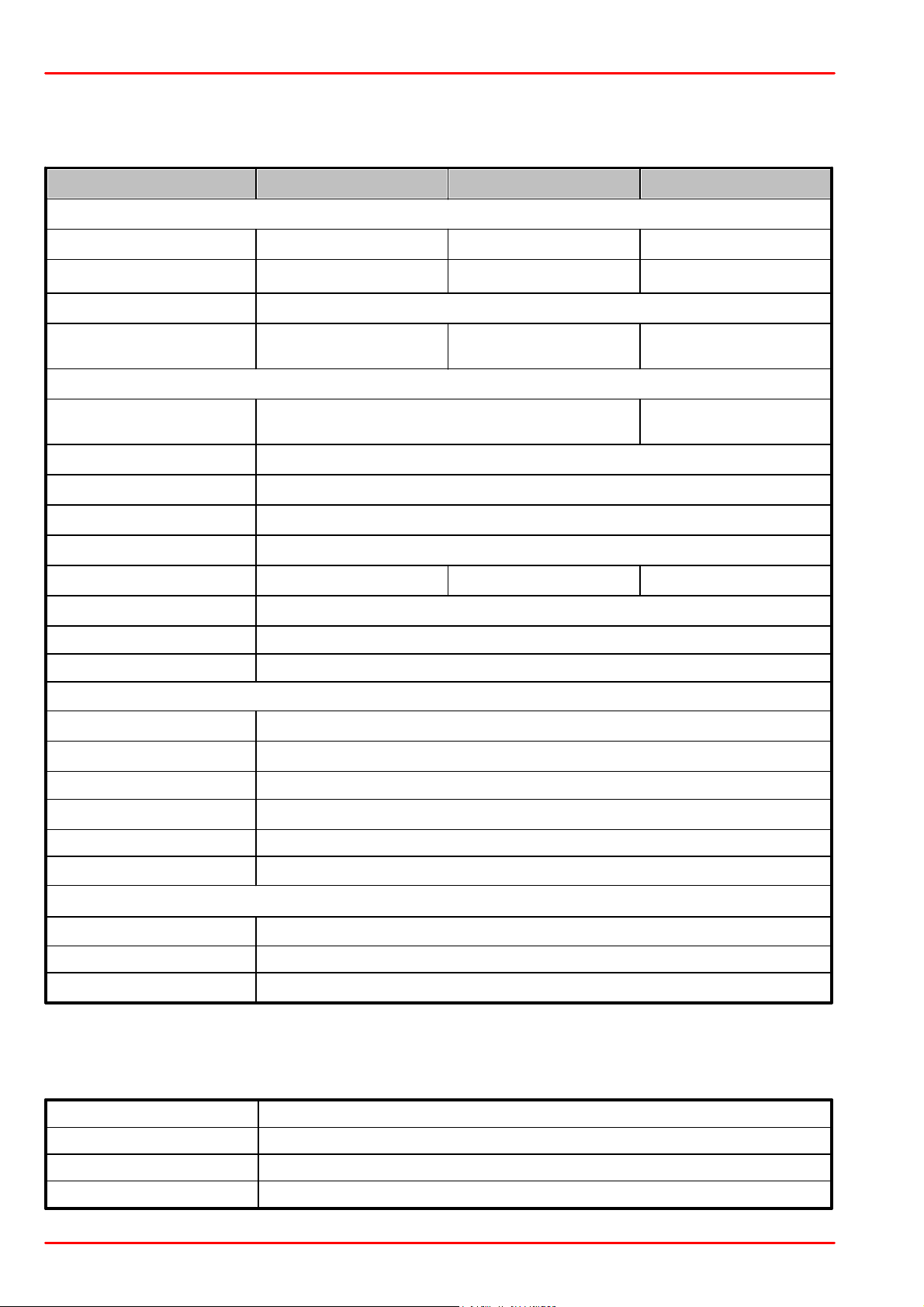
Item #

CCS100

CCS175

CCS200

Optical Specs

Wavelength Range

350 − 700 nm

500 − 1000 nm

200 − 1000 nm

Spectral Accuracy

<0.5 nm FWHM @ 435 nm

<0.6 nm FWHM @ 633 nm

<2 nm FWHM @ 633 nm

Slit (W x H)

20 µm x 2 mm

Grating

1200 Lines/mm,

500 nm Blaze

830 Lines/mm,

800 nm Blaze

600 Lines/mm,

800 nm Blaze

Sensor Specs

Detector Range (CCD

Chip)

350 - 1100 nm

200 - 1100 nm

CCD Pixel Size

8 µm x 200 µm ( 8 µm pitch )

CCD Sensitivity

160 V / ( lx · s )

CCD Dynamic Range

300

CCD Pixel number

3648

Resolution

10 px/nm

6 px/nm

4 px/nm

Integration Time

10 µs − 10 s 3)

Scan Rate Max.

200 Scans/s 2)

S/N ratio

≤ 2000 : 1

External Trigger

Fiber Connector

SMA 905

Trigger Input

SMB

Trigger Signal

TTL

Trigger Frequency Max.

100 Hz

Trigger Pulse Length Min.

0.5 µs

Trigger Delay

8.125 µs ± 125 ns

General Specs

Interface

Hi-Speed USB2.0 (480 Mbit/s)

Dimensions (L x W x H)

122 x 80 x 30 mm

Weight

< 0.4 kg

Operating Temperature

0 to +40 °C

Storage Temperature

-40 to +70 °C

Relative Humidity

Max. 80% up to 31 °C; decreasing to 50% at 40 °C

Operation Altitude

< 3000 m

7 Appendix

7.1 Technical Data

All technical data are valid at 23 ± 5°C and 45 ± 15% rel. humidity (non condensing)

) 220 - 440 nm version available

) integration time 5 ms

) softw are allow s to set up to 60 s. Hot pixels and noise may increase drastically.

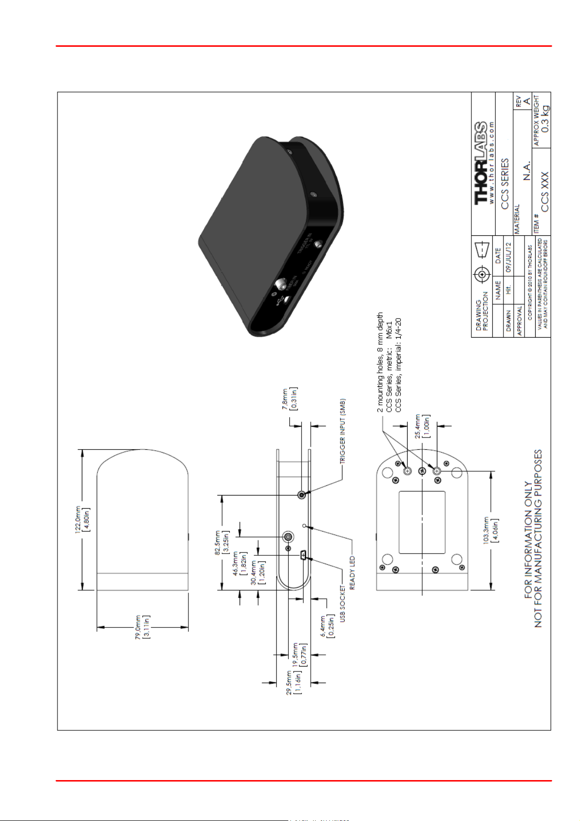
7.2 Dimensions

7 Appendix

CCS Series Spectrometer

7.3 Tutorial

In this section some complementary information is given.

Spectrum File Formats

The Thorlabs OSA software uses a variety of file formats in order to record measurement results.

*.spf2: This is the internal file format to save and load spectrum files from one or more traces. The file header consists of information about the used spectrometer, it's s/n, acquisition settings and trace properties.

*.spc: This file format is a 2D graphic file format, invented by Galactic Industries in 1986 for storage of a variety of different types of data taken from laboratory analytical instrumentation, primarily spectral and chromatographic (trace) data. The SPC format is capable of storing single or multiple arrays and is designed to be general enough to contain most types and styles of data storage such as even X spaced, non-even X spaced, variable record sizes, and 16 or 32 bit data representation. It is also capable of storing arbitrarily large descriptor blocks.

*.jdx: The JCAMP-DX is a commonly used file format for infrared, NMR (nuclear magnetic resonance), and mass spectrometry data introduced by the Joint Committee on Atomic and Molecular Physical Data (JCAMP). More information can be found at http://www.jcamp-dx.org/.

*.csv: The standard comma separated variables file type. It is used to save a single trace. When saving, the separator can be selected to semicolon, comma or tab. Thorlabs OSA software CSV export file has a header of 34 lines with information on the used spectrometer, it's settings, data on the graph and 2 lines for entered manually individual comments. The header is followed by 3648 lines (equal to the 3648 pixels of the CCS spectrometer CCD line) of 2 columns: The first column states the wavelength in [nm], the second the relative intensity.

*.txt: When exporting the active trace, the text file format can be used. A separator (semicolon, comma or tab) must be selected. The exported file contains only the data of the spectra: The first column states the wavelength in [nm], the second the relative intensity.

*.mat: A trace can be saved as a Matlab v.5 file. Level 5 MAT-Files include additional support for multidimensional numeric arrays, character arrays, cell arrays, sparse arrays, objects, and structures.

Image File Formats

A trace can be saved from Thorlabs OSA software in *.bmp, *.png, and *.jpg formats.

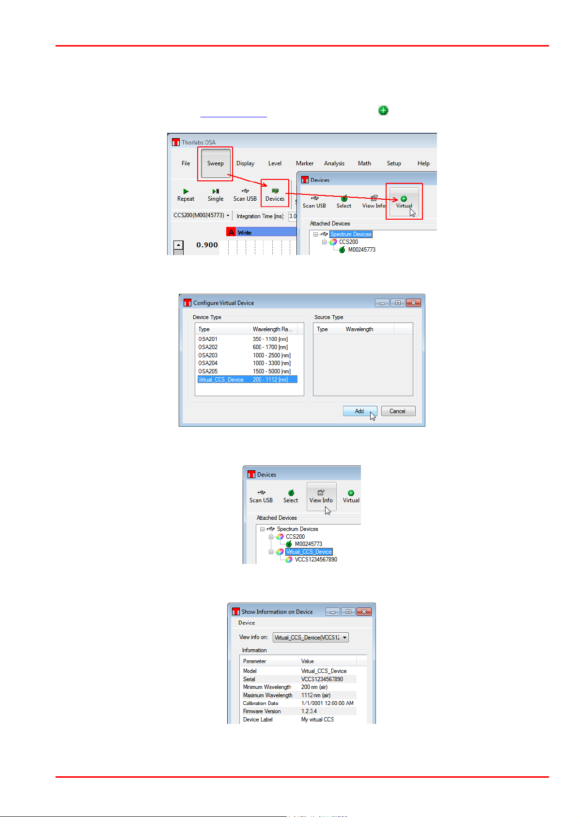
7 Appendix

Virtual Devices

In order to demonstrate the OSA software functionality even without a spectrometer connected, a Virtual Device can be activated. Virtual devices just simulate a spectrometer. Add a virtual device by selecting "Devices" in the Sweep menu, then click the button " Virtual":

A list of available devices comes up:

Select one, the click "Add". The virtual device is listed now:

Select it, then click "View Info" to display it's properties:

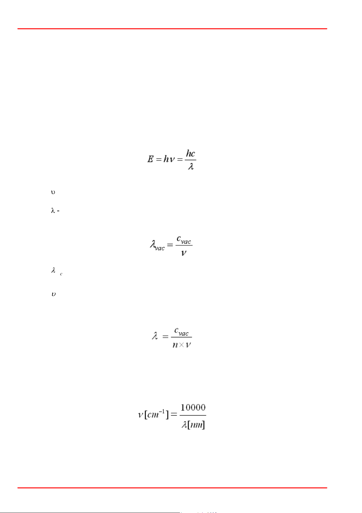
CCS Series Spectrometer

"Settings" file format

The settings of the current spectrum acquisition, that include the spectrum display settings and the settings of the active spectrometer, can be saved as a *.sml file. The file format is XML V 1.0, and the extension was chosen to sml for easy identification.

The file extension is not associated with the SMILE software tool by Simulistic, nor with Single

Markup Language.

Wavelength, Frequency, photon energy and wave number

Photons can be characterized by their frequency, energy, wavelength and wave number, where the wavelength and the wave number depend on the propagation speed in the given medium.

Energy and frequency are related by the equation

with h - Planck constant = 4.13566733 x 10

- frequency

-15

eVs

c - light propagation speed in vacuum = 2.99792458 x 10 8 m/s

- wavelength in vacuum

Wavelength and frequency are correlated by the formula

with

- wavelength in vacuum

vac

- light propagation speed in vacuum = 2.99792458 x 10 8 m/s

vac

- frequency

If the light propagates in a different medium than vacuum, it's propagation speed decreases for a factor called the refraction index. In such case, the wavelength is calculated to

where n is the refraction index. In air, the refraction index is 1.000293, in water - 1.333 The wave number is the spatial frequency of a wave, either in cycles per distance or radians per

unit distance. It can be described as the number of waves that exist over a specified distance. In spectroscopy usually the wave number is given per centimeter (cm -1) and calculated by the formula

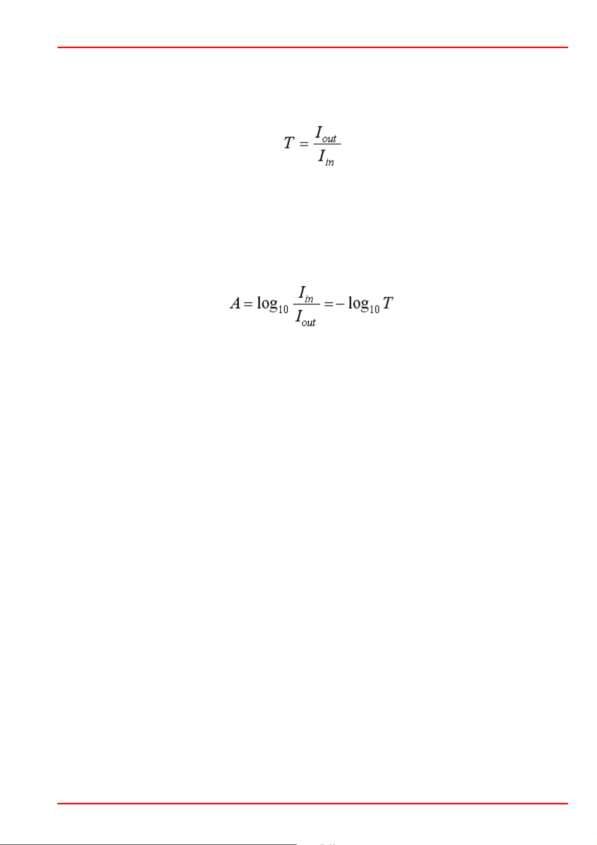
7 Appendix

Transmission and Absorbance

Transmission T (aka transmittance) is the fraction of incident light that passes through a sample, it is calculated as

with I

- intensity at the output of the sample

out

- incident to the sample intensity

Transmittance is stated in %. Absorbance A (aka Optical Density OD) is the logarithmic ratio of the intensity, incident to a

sample, to the intensity, passing through the sample:

with I

- intensity at the output of the sample

out

- incident to the sample intensity

T - transmittance

Absorbance is stated in "absorption units", abbreviated "A.U." or "AU".

CCS Series Spectrometer

7.4 Shortcuts Used in OSA Software

Ctrl+O: Load a spectrum from file to an available trace

Ctrl+S: Save a trace to file

Ctrl+Shift+S: Save all traces to file

Ctrl+P: Print a screen shot

Ctrl+Z: Undo the last math operation performed (if any)

Ctrl+Y: Redo the last math operation undone (if any)

Ctrl+I: Show information about the currently active trace

Ctrl+N: Collect a new single spectrum

Ctrl+R: Start/ Stop repeated measurements

Ctrl+L: Toggle between linear and logarithmic scaling

Ctrl+1: Enable/ disable movable marker number 1 (line marker)

Ctrl+2: Enable/ disable movable marker number 2 (line marker)

Ctrl+3: Enable/ disable movable marker number 3 (level marker)

Ctrl+4: Enable/ disable movable marker number 4 (level marker)

Ctrl+ “+”: Zoom in to the graph

Ctrl+ “-”: Zoom out of the graph

Ctrl+Left Arrow: Move the graph one step to the left

Ctrl+RightArrow: Move the graph one step to the right

Ctrl+PageDown: Set the active trace to the trace after the currently active trace

Ctrl+PageUp: Set the active trace to the trace before the currently active trace

Ctrl+W: Toggle between “Write” and “Fix” on the currently active trace

Delete: Clear the currently active trace

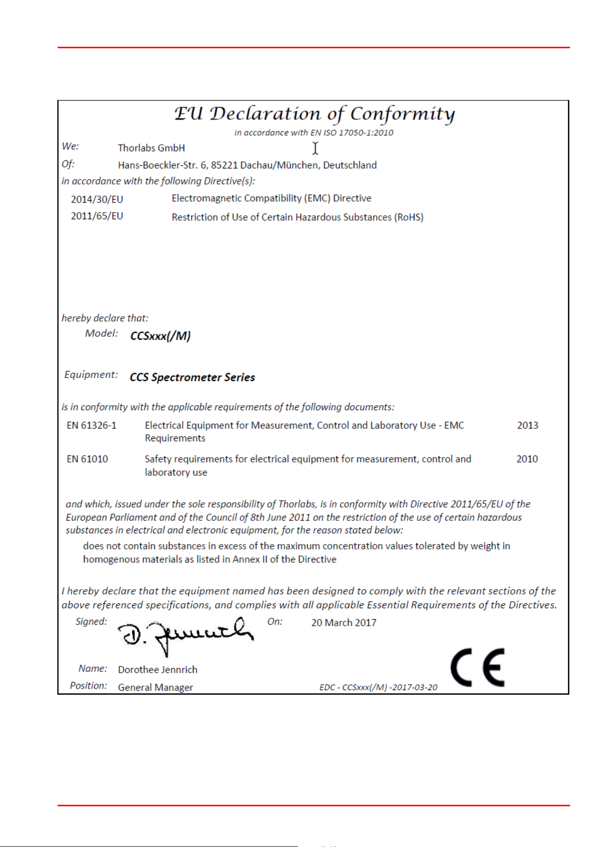
7.5 Certifications and Compliances

7 Appendix

CCS Series Spectrometer

7.6 Warranty

Thorlabs warrants material and production of the CCS Series Spectrometer for a period of 24 months starting with the date of shipment. During this warranty period Thorlabs will see to defaults by repair or by exchange if these are entitled to warranty.

For warranty repairs or service the unit must be sent back to Thorlabs. The customer will carry the shipping costs to Thorlabs, in case of warranty repairs Thorlabs will carry the shipping costs back to the customer.

If no warranty repair is applicable the customer also has to carry the costs for back shipment. In case of shipment from outside EU duties, taxes etc. which should arise have to be carried by the

customer.

Thorlabs warrants the hard- and/or software determined by Thorlabs for this unit to operate faultfree provided that they are handled according to our requirements. However, Thorlabs does not warrant a fault free and uninterrupted operation of the unit, of the software or firmware for special applications nor this instruction manual to be error free. Thorlabs is not liable for consequential damages.

Restriction of Warranty

The warranty mentioned before does not cover errors and defects being the result of improper treatment, software or interface not supplied by us, modification, misuse or operation outside the defined ambient stated by us or unauthorized maintenance.

Further claims will not be consented to and will not be acknowledged. Thorlabs does explicitly not warrant the usability or the economical use for certain cases of application.

Thorlabs reserves the right to change this instruction manual or the technical data of the described unit at any time.

7 Appendix

7.7 Copyright and Exclusion of Reliability

Thorlabs has taken every possible care in preparing this document. We however assume no liability for the content, completeness or quality of the information contained therein. The content of this document is regularly updated and adapted to reflect the current status of the hardware and/or software. We furthermore do not guarantee that this product will function without errors, even if the stated specifications are adhered to.

Under no circumstances can we guarantee that a particular objective can be achieved with the purchase of this product.

Insofar as permitted under statutory regulations, we assume no liability for direct damage, indirect damage or damages suffered by third parties resulting from the purchase of this product. In no event shall any liability exceed the purchase price of the product.

Please note that the content of this document is neither part of any previous or existing agreement, promise, representation or legal relationship, nor an alteration or amendment thereof. All obligations of Thorlabs result from the respective contract of sale, which also includes the complete and exclusively applicable warranty regulations. These contractual warranty regulations are neither extended nor limited by the information contained in this document. Should you require further information on this product, or encounter specific problems that are not discussed in sufficient detail in the document, please contact your local Thorlabs dealer or system installer.

CCS Series Spectrometer

Crossed out

"Wheelie Bin" symbol

7.8 Thorlabs 'End of Life' Policy (WEEE)

As required by the WEEE (Waste Electrical and Electronic Equipment Directive) of the European Community and the corresponding national laws, Thorlabs offers all end users in the EC the possibility to return “end of life” units without incurring disposal charges.

This offer is valid for Thorlabs electrical and electronic equipment

sold after August 13th 2005

marked correspondingly with the crossed out “wheelie bin” logo (see figure below)

sold to a company or institute within the EC

currently owned by a company or institute within the EC

still complete, not disassembled and not contaminated

As the WEEE directive applies to self contained operational electrical and electronic products, this “end of life” take back service does not refer to other Thorlabs products, such as

pure OEM products, that means assemblies to be built into a unit by the user (e. g. OEM laser driver cards)

components

mechanics and optics

left over parts of units disassembled by the user (PCB’s, housings etc.).

Waste treatment on your own responsibility

If you do not return an “end of life” unit to Thorlabs, you must hand it to a company specialized in waste recovery. Do not dispose of the unit in a litter bin or at a public waste disposal site.

WEEE Number (Germany) : DE97581288

Ecological background

It is well known that waste treatment pollutes the environment by releasing toxic products during decomposition. The aim of the European RoHS Directive is to reduce the content of toxic substances in electronic products in the future.

The intent of the WEEE Directive is to enforce the recycling of WEEE. A controlled recycling of end-of-life products will thereby avoid negative impacts on the environment.

7 Appendix

7.9 List of Acronyms

The following acronyms and abbreviations are used in this manual:

CCD Charge-coupled Device CSV Comma Separated Values DLL Dynamic Link Library FCC Federal Communications Commission GUI Graphical User Interface IEC International Electrotechical Commission LL TTL Low Level TTL NA Numerical Aperture OEM Orginal Equipment Manufacturer OSA Optical Spectrum Analyzer OSNR Optical Signal-to-Noise Ratio PC Personal Computer PCB Printed Circuit Board RoHS Restriction of the use of certain hazardous substances in electrical and electronic

equipment SW Software USB Universal Serial Bus VISA Virtual Instrument Software Architecture VME Virtual-8086 Mode Enhancement VXI VMEbus eXtensions for Instrumentation VXIPNP VMEbus eXtensions for Instrumentation Plug aNd Play WEEE Waste Electrical and Electronic Equipment Directive XML eXtensible Markup Language

CCS Series Spectrometer

USA, Canada, and South America

Thorlabs, Inc. 56 Sparta Avenue Newton, NJ 07860 USA Tel: 973-300-3000 Fax: 973-300-3600

www.thorlabs.com www.thorlabs.us (West Coast)

Email: sales@thorlabs.com Support: techsupport@thorlabs.com

UK and Ireland

Thorlabs Ltd. 1 Saint Thomas Place, Ely Cambridgeshire CB7 4EX United Kingdom Tel: +44-1353-654440 Fax: +44-1353-654444

www.thorlabs.com

Email: sales.uk@thorlabs.com Support: techsupport.uk@thorlabs.com

Europe

Thorlabs GmbH Hans-Böckler-Str. 6 85221 Dachau Germany Tel: +49-8131-5956-0 Fax: +49-8131-5956-99

www.thorlabs.de

Email: europe@thorlabs.com

Scandinavia

Thorlabs Sweden AB Bergfotsgatan 7 431 35 Mölndal Sweden Tel: +46-31-733-30-00 Fax: +46-31-703-40-45

www.thorlabs.com

Email: scandinavia@thorlabs.com

France

Thorlabs SAS 109, rue des Côtes 78600 Maisons-Laffitte France Tel: +33-970 444 844 Fax: +33-825 744 800

www.thorlabs.com

Email: sales.fr@thorlabs.com

Brazil

Thorlabs Vendas de Fotônicos Ltda. Rua Riachuelo, 171 São Carlos, SP 13560-110 Brazil Tel: +55-16-3413 7062 Fax: +55-16-3413 7064

www.thorlabs.com

Email: brasil@thorlabs.com

Japan

Thorlabs Japan, Inc. 3-6-3 Kitamachi Nerima-ku, Tokyo 179-0081 Japan Tel: +81-3-6915-7701 Fax: +81-3-6915-7716

www.thorlabs.co.jp

Email: sales@thorlabs.jp

China

Thorlabs China Room A101, No. 100 Lane 2891, South Qilianshan Road Putuo District Shanghai 200331 China Tel: +86-21-60561122 Fax: +86-21-32513480

www.thorlabs.com

Email: chinasales@thorlabs.com

7.10 Thorlabs Worldwide Contacts

7 Appendix

Index

*.bmp

*.mat

*.txt

Analysis

Cut Spectrum

Derivative

66 66*.csv 55*.dll 66*.jdx 66*.jpg 66 66*.png 66*.sml 66*.spc 66*.spf2 66

58, 60.net wrapper dll

4, 66Absorbance

28Add Fixed Marker 37Add Noise

6, 43, 51Amplitude Correction

30 26Automated Peak Search 52Average 52Average and Stop

Duration

Error Handling

Grid density

Help

37 19Devices 16Display Menu 32dominant wa 55Drivers 34

63 19Export Settings 16Export Trace

16File Menu 52Fix 28Fixed Markers

37Gaussian

22, 25

bmp

Calculate

Collect Data

csv

19Background Correct 37Black Body 66

22, 25Center - Span

32chromaticity 16Clear All 28Clear Fixed Marker 34

32, 34Color Analysis

32Color Temperature 37Convert Unit 52Copy From 66 37Curve Fit

Image

Getting Started 13 Parts List 7 Software Installation 8

instrument driver

LabVIEW driver

16, 66

19Import Settings

7Installation

55 37Invert

66jdx 66jpg

55, 56, 58,

60 55LabVIEW samples

CCS Series Spectrometer

Legend

Load

Lorentzian

Main Menu

Math

Noise amplification

Peak Track

Polynomial

56, 58, 60NI VISA Instrument driver

48, 52

25Level 26level marker 25Level Markers 26line marker 16 19Load Settings

22, 25Lock axis

51logarithmic Y axis 34Long term analysis 37

16 28Mark Peaks 26Marker 28Marker Table 66mat 37 52Min (Max) Hold

30, 49Min Peak Height

26movable marker 26movable markers

43 22Normal View

15Operation 37operators 66Optical Density

22Panning 26Peak Search

49 30, 34Peak Track Analysis 22, 48Persistence

66photon energy

66png

16Print

55Programming examples

32purity

Repeat

Restore Factory Defaults

Save All

Search Left

Set Integration Time

Smooth

spf2

Sweep

instruments

Synthetic Spectrum

Threshold

28Remove Fixed Marker 19 19repeated sweep 16Replay

6Requirements 37Resample Data 50

16 16Save Image 19Save Settings 16Save Trace

13, 19Scan USB

26 30Search Range 26Search Right 52Secondary Axis 52Set as Active 51

15, 19, 51Settings Bar

43Setup 70Shortcuts 19Single 37 66spc 64Specifications 66Spectrum File Formats 37Spectrum Math 66 22Split View

33, 34Statistics

15Status Bar 37Stitch Traces 19 16Sweep Menu 19Switch between connected

51Switch Instrument 19switch the active instrument 37

30, 49

7 Appendix

tiff

Transmission

66 16, 52Trace 15, 52Trace Controls

52Trace properties

15Traces

4transmittance 51Trigger Mode 66txt

43User Wavelength Calibration

19, 52, 66View Info

66Virtual Devices

Wavelength Calibration

zoom wavelength range

66wave number 43 43wavelength range 52Write 34Write to file

22X Axis Properties 51X Axis Units

25Y Axis Properties

37Zero Out 22 22Zooming 28Δ Level 28Δ Position

www.thorlabs.com

THORLABS CCS Series, CCS100/M, CCS175/M, CCS200, CCS100 Operation Manual

Specifications and Main Features

Frequently Asked Questions

User Manual

1 General Information

1.1 Safety

1.2 Ordering Codes and Accessories

1.3 Requirements

2 Installation

2.1 Parts List

2.2 Installing Software

3 Getting Started

4 Operating Instruction

4.1 Main Menu

4.1.1 File

4.1.2 Sweep

4.1.3 Display

4.1.4 Level

4.1.5 Marker

4.1.5.1 Movable Markers

4.1.5.2 Fixed Markers

4.1.6 Analysis

4.1.6.1 Peak Track Analysis

4.1.6.2 Color Analysis

4.1.6.3 Statistics

4.1.6.4 Long Term Analysis

4.1.7 Math

4.1.8 Setup

4.1.8.1 Tab Active Device

4.1.8.2 Tab Display

4.1.8.3 Tab Peak Track

4.1.8.4 Tab Reset

4.1.9 Help

4.2 Settings Bar

4.3 Trace Controls

5 Write Your Own Application

5.1 NI VISA Instrument driver 32bit on 32bit systems

5.2 NI VISA Instrument driver 32bit on 64bit systems

5.3 NI VISA Instrument driver 64bit on 64bit systems

6 Maintenance and Service

6.1 Version Information

6.2 Troubleshooting

7 Appendix

7.1 Technical Data

7.2 Dimensions

7.3 Tutorial

7.4 Shortcuts Used in OSA Software

7.5 Certifications and Compliances

7.6 Warranty

7.7 Copyright and Exclusion of Reliability

7.8 Thorlabs 'End of Life' Policy (WEEE)

7.9 List of Acronyms

7.10 Thorlabs Worldwide Contacts