Texas Instruments CBR 2 User Manual

Getting Started with the CBR 2
Sonic Motion Detector

™

Important notice regarding book materials

Texas Instruments and any third party contributors make no
warranty, either express or implied, including but not limited to
any implied warranties of merchantability and fitness for a

particular purpose, regarding any programs or book materials and
makes such materials available solely on an “as-is” basis.

In no event shall Texas Instruments or any third party contributor
be liable to anyone for special, collateral, incidental, or
consequential damages in connection with or arising out of the

purchase or use of these materials, and the sole and exclusive
liability of Texas Instruments, regardless of the form of action, shall
not exceed the purchase price of this product. Moreover, Texas
Instruments shall not be liable for any claim of any kind
whatsoever against the use of these materials by any other party.

 1997, 2004, 2006 Texas Instruments Incorporated. All rights
reserved.

Activity 1 (Graphing Your Motion) and Activity 3 (A Speedy Slide) are used with permission from Vernier Software and Technology. These
activities were adapted from Middle School Science with Calculators by Don Volz and Sandy Sapatka.

Permission is hereby granted to teachers to reprint or photocopy in
classroom, workshop, or seminar quantities the pages in this work
that carry a copyright notice. These pages are designed to be
reproduced by teachers for use in their classes, workshops, or
seminars, provided each copy made shows the copyright notice.
Such copies may not be sold, and further distribution is expressly
prohibited. Except as authorized above, prior written permission
must be obtained from Texas Instruments Incorporated to
reproduce or transmit this work or portions thereof in any other
form or by any other electronic or mechanical means, including
any information storage or retrieval system, unless expressly
permitted by federal copyright law. Send inquiries to this address:
Texas Instruments Incorporated; 7800 Banner Drive, M/S 3918;
Dallas, TX 75251; Attention: Manager, Business Services

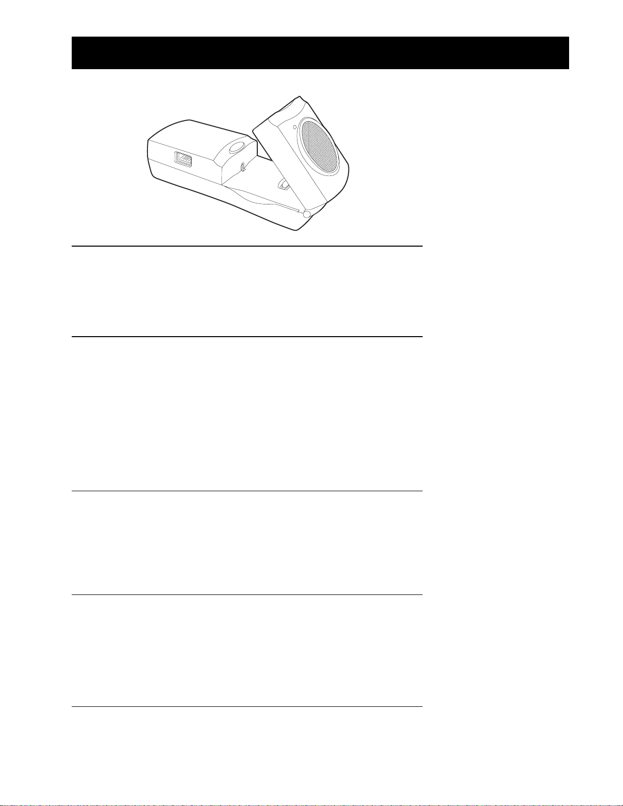
Table of Contents

Introduction

What is the CBR 2™ Sonic Motion Detector? 2

Getting started with the CBR 2™ Sonic Motion Detector 4

Hints for effective data collection 6

Activities with teacher notes and student activity sheets

³ Activity 1 — Graphing your motion linear 10

³ Activity 2 — Match the graph linear 14

³ Activity 3 — A Speedy slide parabolic 18

³ Activity 4 — Bouncing ball parabolic 24

³ Activity 5 — Rolling ball parabolic 28

Teacher information 32

Technical information

Sonic motion detector data is stored in lists 36

EasyData settings 37

Using a CBR 2™ Sonic Motion Detector with a CBL 2™ System
or with CBL 2™ System programs 38

Service information

Batteries 40

In case of difficulty 41

EasyData menu map 42

TI service and warranty 43

© 1997, 2004, 2006 TEXAS INSTRUMENTS INCORPORATED GETTING STARTED WITH THE CBR 2™ SONIC MOTION DETECTOR 1

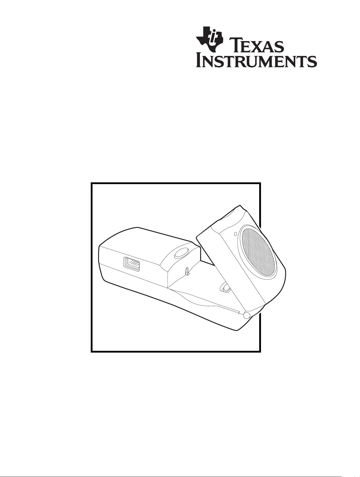
What is the CBR 2™ Sonic Motion Detector?

CBR 2™ (Calculator-Based Ranger™)

sonic motion detector

use with TI-83 Plus, TI-83 Plus Silver Edition,TI-84 Plus, TI-84 Plus Silver Edition

TI-92 Plus, TI-89, TI-89 Titanium, and Voyage™ 200

bring real-world data collection and analysis into the classroom

easy-to-use

What does the CBR 2™ sonic motion detector do?

With the CBR 2™ motion detector and a TI graphing calculator, students can collect, view,
and analyze motion data without tedious measurements and manual plotting.

The

CBR 2™ motion detector lets students explore the mathematical and scientific

relationships between distance, velocity, acceleration, and time using data collected from
activities they perform. Students can explore math and science concepts such as:

0 motion: distance, velocity, acceleration
0 graphing: coordinate axes, slope, intercepts
0 functions: linear, quadratic, exponential, sinusoidal
0 calculus: derivatives, integrals
0 statistics and data analysis: data collection methods, statistical analysis
0 Physics: motion, use with dynamics tracks, pendulum analysis, position, velocity,

acceleration

0 Physical Science: motion experiments

What’s in this guide?

Getting Started with the CBR 2™ Sonic Motion Detector is designed to be a guide for
teachers who do not have extensive calculator experience. It includes quick-start instructions
for using the
activities to explore basic functions and properties of motion. The activities (see pages 10–

31) include many of the following:

0 teacher notes for each activity, plus general teacher information
0 step-by-step instructions
0 a basic data collection activity appropriate for all levels
0 explorations that examine the data more closely, including what-if scenarios
0 suggestions for advanced topics appropriate for precalculus and calculus students
0 a reproducible student activity sheet with open-ended questions appropriate for a wide

range of grade levels

CBR 2™ motion detector, hints on effective data collection, and five classroom

2 GETTING STARTED WITH THE CBR 2™ SONIC MOTION DETECTOR © 1997, 2004, 2006 TEXAS INSTRUMENTS INCORPORATED

What is the CBR 2™ Sonic Motion Detector?

s

¤

s

(cont.)

battery door
(on bottom)

BT (British Telecom) port
to connect to a CBL™,
CBL 2™, or LabPro® unit

to attach a tripod or the
included mounting clamp
(on back)

button

to initiate sampling

tandard threaded socket

USB and I/O ports to connect
to TI graphing calculators using
the included cables

Sensitivity switch to set sensitivity
between Normal and Track
modes (see page 6).

onic sensor to record up
to 200 samples per second
with a range between 15
centimeters and 6 meters
(5.9 inches and 19.7 feet)

pivoting head to aim
sensor accurately

The

CBR 2™ motion detector includes everything you need to begin classroom activities easily and

quickly — just add TI graphing calculators (and readily available props for some activities).

0 sonic motion detector 0 4 AA batteries 0 I/O unit-to-unit cable
0 5 fun classroom activities 0 Standard-B to Mini-A USB cable

(unit-to-

CBR 2™)

©1997, 2004, 2006 TEXAS INSTRUMENTS INCORPORATED GETTING STARTED WITH THE CBR 2™ SONIC MOTION DETECTOR 3

Getting started with the CBR 2™ Sonic Motion Detector

With the CBR 2™ motion detector, you’re just two or three simple steps from the first data
sample!

1111

2222

Download

For TI-83 and TI-84 family calculator users:
Your graphing calculator may have been preloaded with a number of Apps

(software applications), including the EasyData App. Press Πto see the
Apps installed on your calculator. If EasyData is not installed, you may find
the latest version of this App at education.ti.com. If necessary, download the
EasyData App now.

For TI-89, TI-92 Plus, TI-89 Titanium and Voyage™ 200 users:
Obtain the latest RANGER program and install it on your calculator. RANGER

cannot be installed from the
from www.vernier.com or education.ti.com.

CBR 2™ motion detector. RANGER is available

Connect

For TI-83 and TI-84 family calculator users:
Connect the

the Standard-B to Mini-A USB cable (unit-to­cable, and push in firmly at both ends to make a secure connection.

CBR 2™ motion detector to your TI graphing calculator using

CBR 2™) or I/O unit-to-unit

Set the Sensitivity switch to
etc., or to Track mode for use with dynamics tracks and carts.

About the unit-to-

0 Can only be used with the EasyData App.
0 Provides for an auto-launch capability of the EasyData App when

connecting a

0 Provides for an improved physical and more reliable connection than the

I/O unit-to-unit cable.

0 Cannot be used with RANGER, DataMate, or other similar applications.

For TI-89, TI-92 Plus, TI-89 Titanium and Voyage™ 200 users:
Connect the

the I/O unit-to-unit cable and push in firmly at both ends to make a secure
connection.

Set the Sensitivity switch to
etc., or to Track mode for use with dynamics tracks and carts.

CBR 2™ cable:

CBR 2™ motion detector to a TI-84 Plus-family calculator.

CBR 2™ motion detector to your TI graphing calculator using

Normal mode for walking, ball toss, pendulum,

Normal mode for walking, ball toss, pendulum,

4 GETTING STARTED WITH THE CBR 2™ SONIC MOTION DETECTOR © 1997, 2004, 2006 TEXAS INSTRUMENTS INCORPORATED

1111 3333

Run

For TI-83 and TI-84 family calculator users:

For quick results, try
one of the classroom­ready activities in this
guide!

Run the EasyData App on the graphing calculator connected to the
motion detector.

Proceed to step 1, if using a TI-83 Plus-family calculator. For the TI-84 Plus
connected with a unit-to-

1. Turn on the calculator and have it on the home screen.

2. Press Πto display the list of Apps on your graphing calculator.

3. Choose EasyData and press Í.
The opening screen is displayed for about 2–3 seconds, and then the

main screen is displayed.

4. Select

For TI-89, TI-92 Plus, TI-89 Titanium and Voyage™ 200 users:
Run RANGER on the graphing calculator connected to the

detector.

1. Turn on the calculator and have it on the home screen.

2. Press 2 ° to display the list of AppVars on your graphing
calculator.

3. Scroll until you find RANGER. Highlight it and press Í. Type the
closing parenthesis ) and press Í to start the program.

Start (press q) in the main screen to start collecting data.

CBR 2™ cable, perform steps 1 and 4.

CBR 2™ motion

CBR 2™

Important information

0 This guide applies to all TI graphing calculators that can be used with the

CBR 2™ motion detector (see page 2); therefore, you may find that some

of the menu names do not match exactly those on your calculator.

0 When setting up activities, ensure that the CBR 2™ motion detector is

securely anchored and that the cord cannot be tripped over.

0 Always disconnect the CBR 2™ motion detector from the calculator

before storing it.

For TI-83 and TI-84 family calculator users:

0 Always exit the EasyData App using the Quit option. The EasyData App

performs a proper shutdown of the
choose
initialized for the next time you use it.

0 EasyData is launched automatically when the unit-to-CBR 2™ cable is

connected from a TI-84 Plus or TI-84 Plus Silver Edition graphing
calculator to a

For TI-89, TI-92 Plus, TI-89 Titanium and Voyage™ 200 users:

0 EasyData will not run on your calculator. RANGER is the only program

available to simplify the data collection process from the CBR 2.

© 1997, 2004, 2006 TEXAS INSTRUMENTS INCORPORATED GETTING STARTED WITH THE CBR 2™ SONIC MOTION DETECTOR 5

Quit. This ensures that the CBR 2™ motion detector is properly

CBR 2™ motion detector.

CBR 2™ motion detector when you

Hints for effective data collection

Getting better samples

How does the CBR 2™ sonic motion detector work?

Understanding how a sonic motion detector works can help you get better data plots. The
motion detector sends out an ultrasonic pulse and then measures how long it takes for that
pulse to return after bouncing off the closest object.

The

CBR 2™ motion detector, like any sonic motion detector, measures the time interval

between transmitting the ultrasonic pulse and the first returned echo, but the
motion detector has a built-in microprocessor that does much more. When the data is
collected, the
motion detector using a speed-of-sound calculation. Then it computes the first and second
derivatives of the distance data with respect to time to obtain velocity and acceleration data.
It stores these measurements in lists.

Object size

Using a small object at a far distance from the CBR 2™ motion detector decreases the
chances of an accurate reading. For example, at 5 meters, you are much more likely to
detect a soccer ball than a ping-pong ball.

CBR 2™ motion detector calculates the distance of the object from the CBR 2™

CBR 2™

Minimum range

When the CBR 2™ motion detector sends out a pulse, the pulse hits the object, bounces
back, and is received by the

CBR 2™ motion detector. If an object is closer than 15

centimeters (about six inches), consecutive pulses may overlap and be misidentified by the

CBR 2™ motion detector. The plot would be inaccurate, so position the CBR 2™ motion

detector at least 15 centimeters away from the object.

Maximum range

As the pulse travels through the air, it loses its strength. After about 12 meters (6 meters on
the trip to the object and 6 meters on the trip back to the
return echo may be too weak to be reliably detected by the
limits the typical reliably effective distance from the

CBR 2™ motion detector to the object to

CBR 2™ motion detector), the

CBR 2™ motion detector. This

less than 6 meters (about 20 feet).

Sensitivity switch

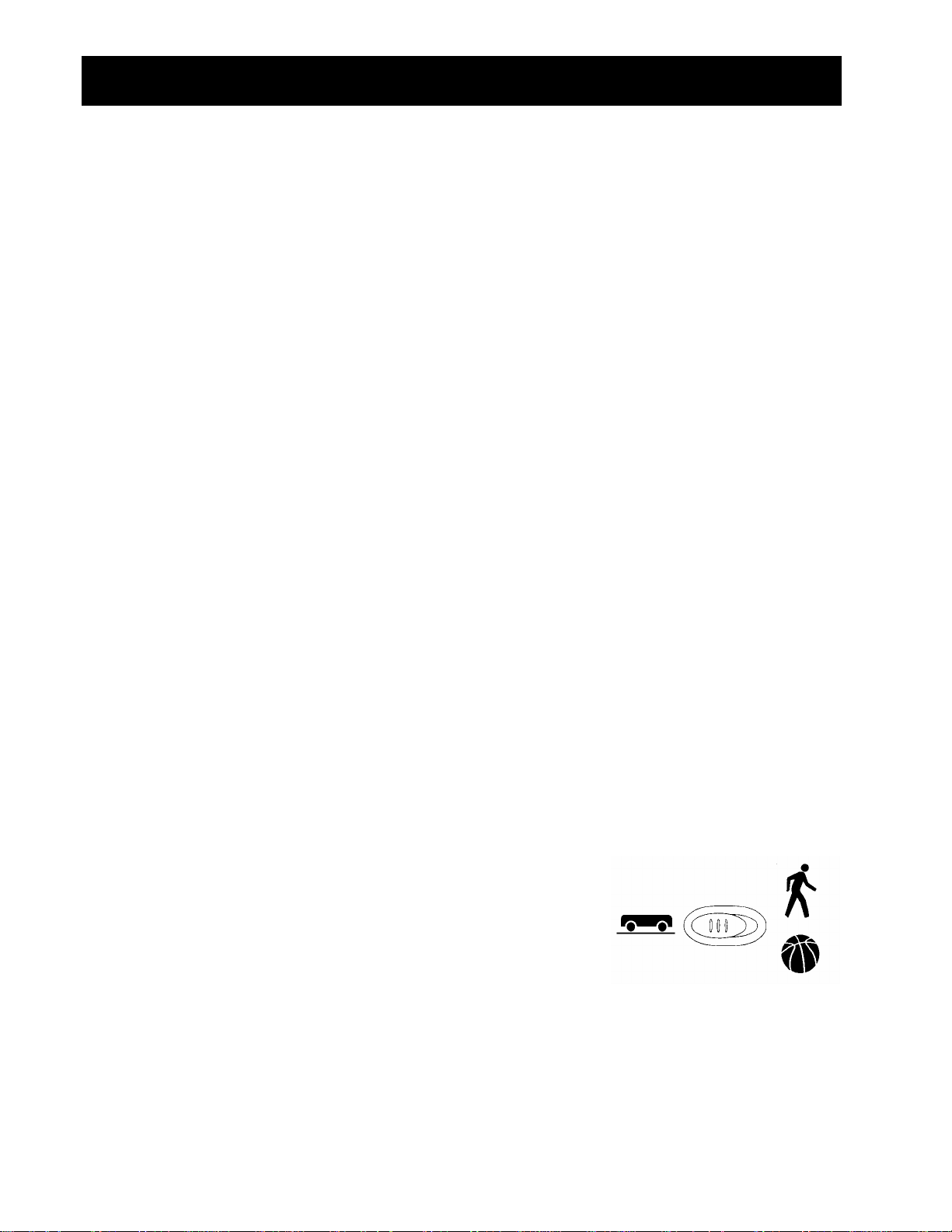
The sensitivity switch has two modes—Track and Normal.
The Track mode is intended for activities using dynamics
tracks and carts; the Normal mode is intended for all other

Track Normal

% &

activities, such as, walking, ball toss, bouncing ball,
pendulum, etc.

If you are getting lots of extra noise in your data, the sensitivity switch may be in the Normal
mode. Moving the sensitivity switch to the Track position, will reduce the sensitivity of the
sensor and may produce better data.

6 GETTING STARTED WITH THE CBR 2™ SONIC MOTION DETECTOR © 1997, 2004, 2006 TEXAS INSTRUMENTS INCORPORATED

Hints for effective data collection

s

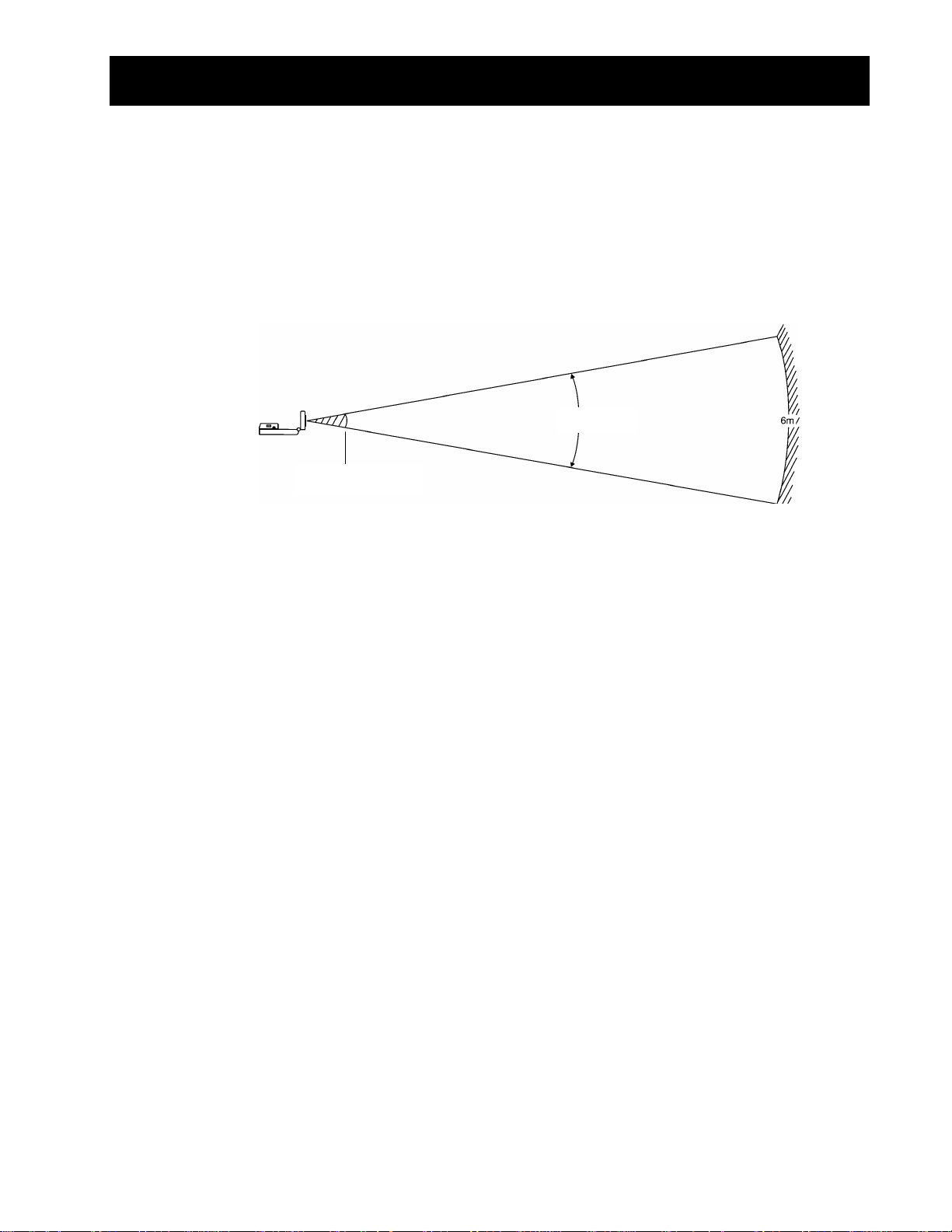
The clear zone

The path of the CBR 2™ motion detector beam is not a narrow, pencil-like beam, but fans
out in all directions up to 15° from center in a 30° cone-shaped beam.

To avoid interference from other objects in the vicinity, try to establish a clear zone in the
path of the
target do not get recorded by the
records the closest object in the clear zone.

Reflective surfaces

CBR 2™ motion detector beam. This helps ensure that objects other than the

CBR 2™ motion detector. The CBR 2™ motion detector

15 centimeter

(cont.)

30°

Some surfaces reflect pulses better than others. For example, you might see better results
with a relatively hard, smooth surfaced ball than with a tennis ball. Conversely, samples
taken in a room filled with hard, reflective surfaces are more likely to show stray data points.
Measurements of irregular surfaces (such as a toy car or a student holding a calculator while
walking) may appear uneven.

A Distance-Time plot of a nonmoving object may have small differences in the calculated
distance values. If any of these values map to a different pixel, the expected flat line may
show occasional blips. The Velocity-Time plot may appear even more jagged, because the
change in distance between any two points over time is, by definition, velocity.

© 1997, 2004, 2006 TEXAS INSTRUMENTS INCORPORATED GETTING STARTED WITH THE CBR 2™ SONIC MOTION DETECTOR 7

Hints for effective data collection

(cont.)

EasyData settings (for TI-83, TI-83 Plus, TI-84, and TI-84 Plus users only)

Setup data collection for Time Graph

Experiment length is the total time in seconds to complete all sampling. It’s determined by
the number of samples multiplied by the sample interval.

Enter a number between 0.05 (for very fast moving objects) and 0.5 seconds (for very slow
moving objects).

Note: See “To set up the calculator for data collection” on page 12 for detailed information
about how to change settings.

Menu name Description Default setting

Sample Interval Measures time between samples in seconds. 0.05
Number of Samples Total number of samples to collect. 100
Experiment Length Length of the experiment in seconds. 5

Starting and stopping

To start sampling, select Start (press q). Sampling will automatically stop when the
number of samples set in the
detector will then display a graph of the sampled data on the graphing calculator.

Time Graph Settings menu is reached. The CBR 2™ motion

To stop sampling before it automatically stops, select

Stop (press and hold q) at any time

during the sampling process. When sampling stops, a graph of the sampled data is
displayed.

Noise—what is it and how do you get rid of it?

When the CBR 2™ motion detector receives signals reflected from objects other than the
primary target, the plot shows erratic data points (noise spikes) that do not conform to the
general pattern of the plot. To minimize noise:

0 Make sure the CBR 2™ motion detector is pointed directly at the target. Try adjusting the

sensor head while viewing live data on the home-screen meter. Make sure the reading
you receive is appropriate before starting an activity or experiment.

0 Try to sample in a clutter-free space (see the clear zone drawing on page 7).
0 Choose a larger, more reflective object or move the object closer to the CBR 2™ (but

farther than 15 centimeters).

0 When using more than one CBR 2™ motion detector in a room, one group should

complete a sample before the next group begins their sample.

0 Try moving the sensitivity switch to the Track position to reduce the sensitivity of the

sensor.

8 GETTING STARTED WITH THE CBR 2™ SONIC MOTION DETECTOR © 1997, 2004, 2006 TEXAS INSTRUMENTS INCORPORATED

Hints for effective data collection

Speed of sound

The approximate distance to the object is calculated by assuming a nominal speed of sound.
However, actual speed of sound varies with several factors, most notably the air
temperature.

The

CBR 2™ motion detector has a built-in temperature sensor to automatically compensate

for changes in the speed of sound due to the temperature of the surrounding air. The
temperature conversion from 0° to 40° Celsius, at standard pressure, is fairly linear at about
+0.6 meters/second per degree Celsius. The speed of sound increases from about 331
meters/second at 0° Celsius to about 355 meters/second at 40° Celsius. These speeds
assume a relative humidity of 35% (dry air).

(cont.)

When using the EasyData App with the
compensation will take place when collecting motion data. The sensor is located underneath
the holes on the back of the
not cover these holes with something that is of a different temperature from the
surrounding ambient temperature.

CBR 2™ motion detector; therefore, when collecting data, do

CBR 2™ motion detector, this temperature

Using the CBR 2™ sonic motion detector without the EasyData application

You can use the CBR 2™ unit as a sonic motion detector with a CBL 2™ system or with
programs other than EasyData.

Using the I/O unit-to-unit cable, the
calculators that do not have the EasyData App installed but do have the
the RANGER program. The

CBR™ motion detector when sample data is collected using the CBL/CBR App and/or the

RANGER program.

CBL/CBR App can be used on most older TI-83 Plus calculators. The CBL/CBR App is

The
available for downloading at education.ti.com and allows you to collect motion data using
the I/O unit-to-unit cable on the

The RANGER program, which is part of the
allows you to collect motion data using the I/O unit-to-unit cable. Many TI Explorations
workbooks use the RANGER program. (The RANGER program is the only program available
for use with the TI-89, TI-92 Plus, TI-89 Titanium, and Voyage™ 200 to perform activities
like Ball Bounce and Graph Match.)

CBR 2™ motion detector will provide the same functionality as a

CBR 2™ motion detector can be used with graphing

CBL/CBR App and/or

CBR 2™ motion detector.

CBL/CBR App and available for other calculators,

You can also use
Use the DataMate App that comes with the
detector
For more information about this cable visit the TI webstore at education.ti.com.

© 1997, 2004, 2006 TEXAS INSTRUMENTS INCORPORATED GETTING STARTED WITH THE CBR 2™ SONIC MOTION DETECTOR 9

through a CBL 2™ system. A special CBL-to-CBR cable is required to use this system.

CBR 2™ unit as a motion sensor with your CBL 2™ data collection device.

CBL 2™ system to operate the CBR 2™ motion

Activity 1—Graphing Your Motion Notes for Teachers

Concepts

Function explored: linear

Materials

Ÿ calculator (see page 2 for available models)
Ÿ CBR 2™ motion detector
Ÿ unit-to-CBR 2™ or I/O unit-to-unit cable
Ÿ EasyData application or RANGER program
Ÿ Masking tape
Ÿ Meter stick

Hints

This experiment may be the first time your students
use the CBR 2™ motion detector. A little coaching on
its use now will save time later in the year as the
CBR 2™ motion detector is used in many experiments.
The following are hints for effective use of the
CBR 2™ motion detector:

0 In using the CBR 2™ motion detector, it is

important to realize that the ultra sound is emitted
in a cone about 30° wide. Anything within the
cone of ultrasound can cause a reflection and
possibly an accidental measurement. A common
problem in using motion detectors is getting
unintentional reflections from a desk or chair in
the room.

0 Often unintended reflections can be minimized by

tilting the CBR 2™ motion detector slightly.

0 If you begin with a velocity or acceleration graph

and obtain a confusing display, switch back to a
distance graph to see if it makes sense. If not, the
CBR 2™ motion detector may not be properly
targeting the target.

0 The CBR 2™ motion detector does not properly

detect objects closer than 15 cm. The maximum
range is about 6 m, but stray objects in the wide
detection cone can be problematic at this distance.

0 Sometimes a target may not supply a strong

reflection of the ultrasound. For example, if the
target is a person wearing a bulky sweater, the
resulting graph may be inconsistent.

0 If the velocity and acceleration graphs are noisy, try

to increase the strength of the ultrasonic reflection
from the target by increasing the target’s area.

You may want to have your students hold a large
book in front of them as they walk in front of the
CBR 2™ motion detector. This will produce better
graphs because it smoothes out the motion.

Typical plots

Distance vs. Time

Matching Distance vs. Time

Answers to questions

9. The slope of the portion of the graph
corresponding to movement is greater for the
faster trial.

Results will probably vary between groups as they

may walk at different rates.

Walking towards the motion detector will produce

a negative slope. While walking away from the
motion detector will produce a positive slope.

12. Note that the slope is close to zero (if not zero)
when standing still. The slope should be zero, but
expect small variation due to the variation in
collected data.

10 GETTING STARTED WITH THE CBR 2™ SONIC MOTION DETECTOR © 2000 VERNIER SOFTWARE & TECHNOLOGY

Activity 1—Graphing Your Motion Linear

Graphs made using a CBR 2™ motion detector can be used to study motion. In this experiment, you
will use a

Objectives

Data collection: Distance vs. Time Graphs

CBR 2™ motion detector to make graphs of your own motion.

In this experiment, you will:

0 use a motion detector to measure distance and velocity
0 produce graphs of your motion
0 analyze the graphs you produce

Ê Place a CBR 2™ motion detector to a tabletop facing an area free of furniture and other

objects. The
above your waist level.

CBR 2™ motion detector should be at a height of about 15 centimeters

walk back and forth in

front of the CBR 2™

motion detector

Ë Use short strips of masking tape on the floor to mark the 1-m, 2-m, 3-m, and 4-m

distances from the

CBR 2™ motion detector.

Ì Connect the CBR 2™ motion detector to the calculator using an appropriate cable (see

below) and firmly press in the cable ends.

0 If TI-83 Plus, TI-89, TI-92 Plus, TI-89 Titanium, Voyage™ 200, use an I/O unit-to-unit

cable

0 If TI-84 Plus, use a Standard-B to Mini-A USB cable (unit-to-CBR 2™)

Í On the calculator, press Œ and select EasyData to launch the EasyData App or press

2 ° and select RANGER if you are using a calculator that does not operate
with EasyData.

Note: EasyData will launch automatically if the

a TI-84 Plus using a unit-to-

© 2000 VERNIER SOFTWARE & TECHNOLOGY GETTING STARTED WITH THE CBR 2™ SONIC MOTION DETECTOR 11

CBR 2™ cable.

CBR 2™ motion detector is connected to

Activity 1—Graphing Your Motion

Î To set up the calculator for data collection using EasyData:

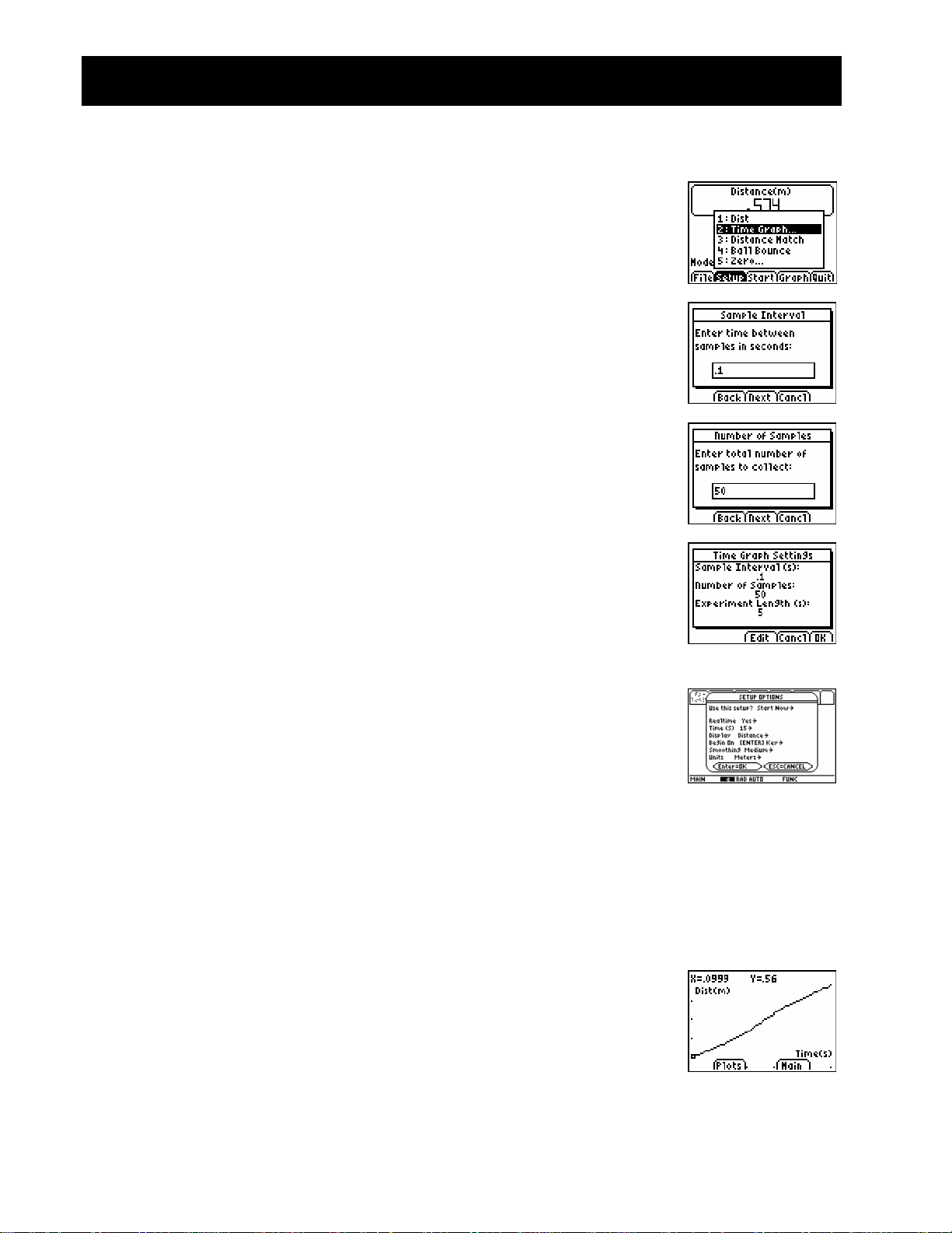
a. Select Setup (press p) to open the Setup menu.

(cont.)

Linear

TI-83/84 Family users

b. Press 2 to select

Settings

c. Select Edit (press q) to open the

window.

d. Enter 0.1 to set the time between samples to 1/10 second.

e. Select

Samples

f. Enter 50 to set the number of samples to collect.

The experiment length will be 5 seconds (number of

samples multiplied by the sample interval).

g. Select

settings.

h. Select

screen.

Next (press q) to advance to the Number of

dialog window.

Next (press q) to display a summary of the new

OK (press s) to return to the main screen.

2: Time Graph to open the Time Graph

Sample Interval dialog

To set up the calculator for data collection using RANGER:

TI-89/Titanium/92+/V200

a. Choose 1:Setup/Sample… from the Main Menu.

b. Use C D to move to each parameter line. Use B to view

the options for each parameter. To change a parameter,
highlight the options and press ¸.

Ï Explore making distance vs. time graphs.

a. Stand at the 1.0-m mark, facing away from the

motion detector.

b. Signal your partner to select

c. Slowly walk to the 2.5-m mark and stop.

d. When data collection ends, a graph plot is displayed.

Start (press p).

CBR 2™

12 GETTING STARTED WITH THE CBR 2™ SONIC MOTION DETECTOR © 2000 VERNIER SOFTWARE & TECHNOLOGY

Activity 1—Graphing Your Motion

e. Sketch your graph on the empty graph provided.

f. Pick two points on the graph and determine the slope from

the x and y-coordinates.

Point 1:________ Point 2: ________ Slope:___________

g. Select

Ð Repeat Step 6, this time standing on the 2.5m-mark and walk

towards the 1.0m-mark. One time walking slowly, and again
walking more quickly.

Point 1:________ Point 2: ________ Slope:___________

Ñ Sketch your new plots on the empty graph provided.

Ò Describe the differences between your graphs (step 6e and step 8)

___________________________________________________________________________

___________________________________________________________________________

Main (press r) to return to the main screen.

(cont.)

Linear

___________________________________________________________________________

Ó Repeat Step 6, while standing still on the 2.5m-mark.

Ô Sketch your new plot on the empty graph provided.

Õ Calculate an approximate slope for all your graphs.

© 2000 VERNIER SOFTWARE & TECHNOLOGY GETTING STARTED WITH THE CBR 2™ SONIC MOTION DETECTOR 13

Activity 2—Match the Graph Notes for Teachers

Concepts

Function explored: linear
Distance Match introduces the real-world concepts of

distance and time—or more precisely, the concept of
distance versus time.

In Explorations, students are asked to convert their
rate of walking in meters per second to kilometers per
hours.

Once they have mastered the Distance-Time match,
challenge your students to a Velocity-Time match.

Materials

Ÿ calculator (see page 2 for available models)
Ÿ CBR 2™ motion detector
Ÿ unit-to-CBR 2™ or I/O unit-to-unit cable
Ÿ EasyData application or RANGER program

A TI ViewScreené panel allows other students to
watch—and provides much of the fun of this activity.

Hints

Students really enjoy this activity. Plan adequate time
because everybody will want to try it!

This activity works best when the student who is
walking (and the entire class) can view his or her
motion projected on a wall or screen using the TI
ViewScreené panel.

Guide the students to walk in-line with the CBR 2™
motion detector; they sometimes try to walk sideways
(perpendicular to the line to the CBR 2™ motion
detector) or even to jump up!

Instructions suggest that the activity be done in
meters, which matches the questions on the student
activity sheet.

See pages 6–9 for hints on effective data collection.

Typical plot

Typical answers

1. time (from start of sample); seconds; 1 second;
distance (from the CBR 2™ motion detector to the
object); meters; 1 meter

2. the y-intercept represents the starting distance

3. varies by student

4. backward (increase the distance between the
CBR 2™ motion detector and the object)

5. forward (decrease the distance between the
CBR 2™ motion detector and the object)

6. stand still; zero slope requires no change in y
(distance)

7. varies by graph; @yà3.3

8. varies by graph; @yà1

9. the segment with the greatest slope (positive or
negative)

10. this is a trick question—the flat segment, because
you don’t move at all!

11. walking speed; when to change direction and/or
speed

12. speed (or velocity)

13. varies by graph (example: 1.5 meters in 3 seconds)

14. varies by graph; example: 0.5 metersà1 second

example: (0.5 meters à 1 second) Q (60 seconds à

1 minute) = 30 meters à minute

example: (30 meters à 1 minute) Q (60 minutes à 1

hour) = 1800 meters à hour

example: (1800 meters à 1 hour) Q (1 kilometer à

1000 meters) = 1.8 kilometers à hour.

Have students compare this last number to the

velocity of a vehicle, say 96 kilometers à hour
(60 miles per hour).

15. varies by graph; sum of the @y for each line
segment.

Distance vs. Time

Matching Distance vs. Time

14 GETTING STARTED WITH THE CBR 2™ SONIC MOTION DETECTOR © 2004 TEXAS INSTRUMENTS INCORPORATED

Activity 2—Match the Graph Linear

Data collection

Ê Hold the CBR 2™ motion detector in one hand, and the calculator in the other. Aim the

sensor directly at a wall.

Hints: The maximum distance of any graph is 6 meters (about 20 feet) from the

CBR 2™ motion detector. The minimum range is 15 centimeters (about 6 inches). Make

sure that there is nothing in the clear zone (see page 7).

Ë Run the EasyData application or RANGER program.

Ì EasyData Users: From the Setup menu choose 3:Distance Match. Distance Match

automatically takes care of the settings.

RANGER Users: From the Main Menu, choose 3:Applications. Choose the distance units,

then choose 1:Distance Match, and follow the directions on the screen.

Í Select Start (press q) and follow the instructions on the

screen.

Î Select Next (press q) to display the graph to match. Take a

moment to study the graph. Answer questions 1 and 2 on the
activity sheet.

Note: The graph to match will be different each time step 4 and

step 5 are performed.

© 1997, 2004, 2006 TEXAS INSTRUMENTS INCORPORATED GETTING STARTED WITH THE CBR 2™ SONIC MOTION DETECTOR 15

Activity 2—Match the Graph

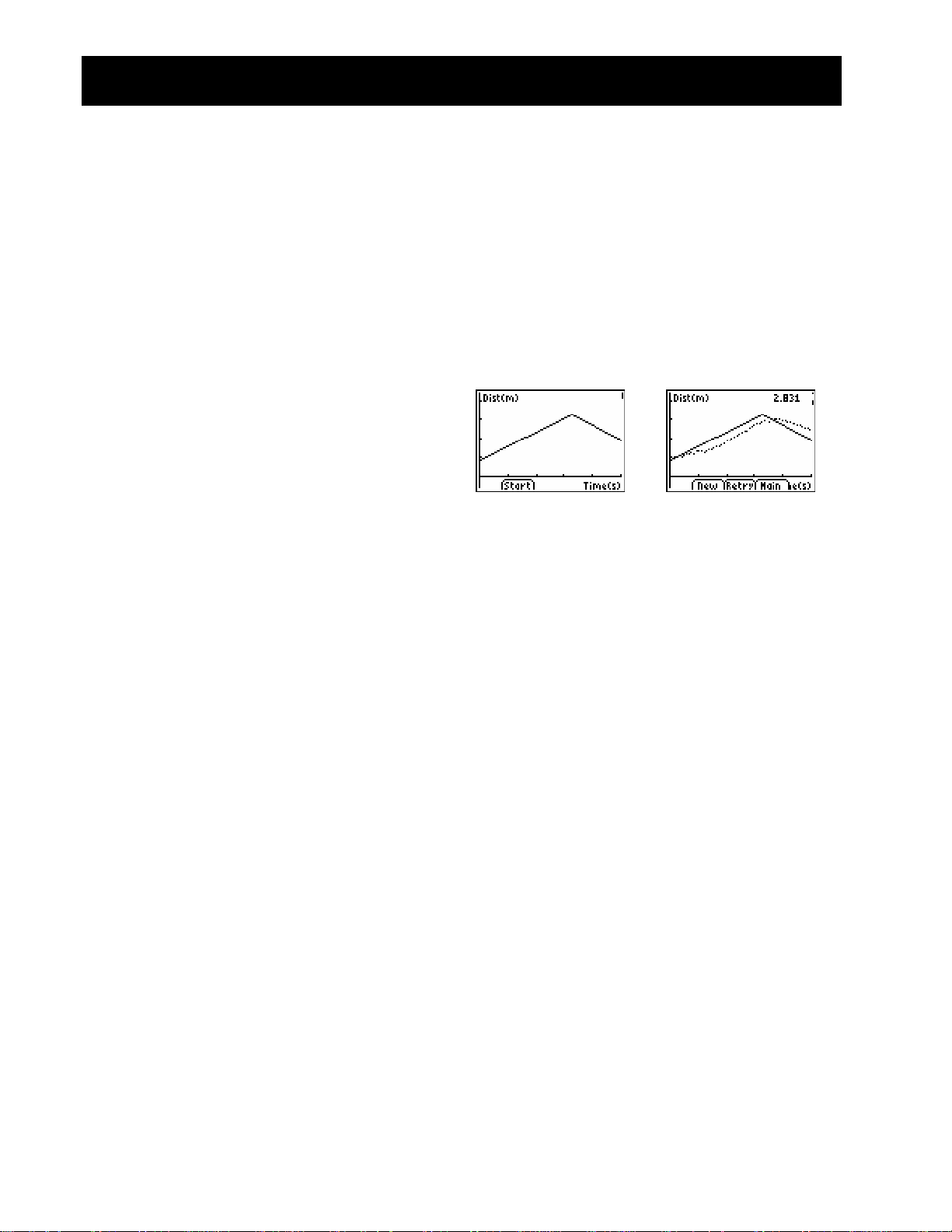
Ï Position yourself where you think the graph begins. Select Start (press p) to begin

data collection. You can hear a clicking sound and see the green light as the data is
collected.

Ð Walk backward and forward, and try to match the graph. Your position is plotted on the

screen.

Ñ When the sample is finished, examine how well your “walk” matched the graph, and

then answer question 3.

Ò Select Retry (press q) to redisplay the same graph to match. Try to improve your

walking technique, and then answer questions 4, 5, and 6.

Explorations

In Distance Match, all graphs are comprised of three straight-line segments.

Ê Select New (press p) to display a new graph to match. Study the first segment

and answer questions 7 and 8.

Ë Study the entire graph and answer questions 9 and 10.

(cont.)

Linear

Ì Position yourself where you think the graph begins, select Start (press p) to begin

data collection, and try to match the graph.

Í When the sampling stops, answer questions 11 and 12.

Î Select New (press p) to display another new graph to match.

Ï Study the graph and answer questions 13, 14, and 15.

Ð Select New (press p) and repeat the activity, if desired, or select Main (press

r) to return to the main screen

Ñ Select Quit (press s) and OK (press s) to exit the EasyData App.

16 GETTING STARTED WITH THE CBR 2™ SONIC MOTION DETECTOR © 1997, 2004, 2006 TEXAS INSTRUMENTS INCORPORATED

Activity 2—Match the Graph

Name ___________________________________

Data collection

1. What physical property is represented along the x-axis? _____________________________________

What are the units?

What physical property is represented along the y-axis? _____________________________________

What are the units?

2. How far from the CBR 2™ motion detector do you think you should stand to begin? ____________

3. Did you begin too close, too far, or just right? _____________________________________________

4. Should you walk forward or backward for a segment that slopes up? _________________________

Why? _______________________________________________________________________________

5. Should you walk forward or backward for a segment that slopes down? _______________________

Why? _______________________________________________________________________________

6. What should you do for a segment that is flat? ____________________________________________

How far apart are the tick marks? ________________

How far apart are the tick marks? ________________

Why? _______________________________________________________________________________

Explorations

7. If you take one step every second, how long should that step be? ____________________________

8. If, instead, you take steps of 1 meter (or 1 foot) in length, how many steps must you take? _______

9. For which segment will you have to move the fastest? ______________________________________

Why? _______________________________________________________________________________

10. For which segment will you have to move the slowest? _____________________________________

Why? _______________________________________________________________________________

11. In addition to choosing whether to move forward or backward, what other factors entered into

matching the graph exactly? ____________________________________________________________

____________________________________________________________________________________

12. What physical property does the slope, or steepness of the line segment, represent? ____________

13. For the first line segment, how many meters must you walk in how many seconds? _____________

14. Convert the value in question 13 (the velocity) to metersà1 second: ___________________________

Convert to metersàminute: _____________________________________________________________

Convert to metersàhour: _______________________________________________________________

Convert to kilometersàhour: ____________________________________________________________

15. How far did you actually walk? _________________________________________________________

© 1997, 2004, 2006 TEXAS INSTRUMENTS INCORPORATED GETTING STARTED WITH THE CBR 2™ SONIC MOTION DETECTOR 17

Activity 3—A Speedy Slide Notes for Teachers

Concepts

Function explored: parabolic
The motion of sliding down a playground slide is used

to illustrate the real-world concept of changing
velocity due to friction.

Materials

Ÿ calculator (see page 2 for available models)
Ÿ CBR 2™ motion detector
Ÿ unit-to-CBR 2™ or I/O unit-to-unit cable
Ÿ EasyData application or RANGER program
Ÿ Playground slide

Hints

The use of a playground area with several slides is
preferable for this experiment. The slides should be
straight. Slides with other shapes could be used in an
extension. For safety reasons, remind your students
not to attempt to pass each other while on the slide
steps.

You may wish to carry the interfaces, calculators, and
motion detectors to the playground area in a box or
boxes, and distribute the equipment to your students
there. Remind your students that the Motion Detector
does not properly detect objects closer than 15cm.

Depending on the type of slides that are available, you
may wish to change the way your students position
themselves for data collection. Some slides have large
platforms where the student with the Motion
Detector and the student with the calculator and
interface can be located.

Students can use wax paper, slippery cloth, sand, and
other materials to increase their speed. To enable your
students to be prepared, be sure to alert them to Part
II in advance.

Typical plots

A Speedy Slide

Typical answers

1. See the Sample Results.

2. In the Sample Results, the Part 2 speed was 0.90
m/sec greater than the Part 1 speed. Wax paper
was used to decrease friction and increase speed.

3. Answers will vary. Speeds will differ because of
differences such as contact area, weight,
streamlining, and the use of low-friction materials.

4. Answers will vary.

5. Increasing the height of the slide should increase
speed.

6. The stone dropped from the top of the slide
should hit the ground first because friction and the
incline of the slide slow the rolling stone more.

7. The level part at the bottom of a slide slows sliders
and prevents injuries.

Extensions

Design and carry out a plan to measure speed or
velocity on a different piece of playground equipment.

Have a contest to see who in the class or group can
obtain the greatest speed going down a slide.

Sample results

Speed (m/sec)

Trial 1 Trial 2 Trial 3 Average

Part 1

Part 2

18 GETTING STARTED WITH THE CBR 2™ SONIC MOTION DETECTOR © 2000 VERNIER SOFTWARE & TECHNOLOGY

1.97 2.02 2.00 2.00

2.80 3.07 2.82 2.90

Activity 3—A Speedy Slide Parabolic

You have been familiar with playgrounds and slides since you were a small child. The force of gravity pulls
you down a slide. The force of friction slows you down. In the first part of this experiment, you will use a

CBR 2™ motion detector to determine your speed or velocity going down a playground slide. In the

second part, you will experiment with different ways to increase your speed going down the slide.

Objectives

In this experiment, you will:

0 use a CBR 2™ motion detector to determine your speed going down a slide
0 experiment with ways to increase your speed going down the slide
0 explain your results

Data collection, Part 1, Sliding Speed

Ê Connect the CBR 2™ motion detector to the calculator using an appropriate cable (see

below) and firmly press in the cable ends.

0 If TI-83 Plus, TI-89, TI-92 Plus, TI-89 Titanium, Voyage™ 200, use an I/O unit-to-

unit cable

0 If TI-84 Plus, use a Standard-B to Mini-A USB cable (unit-to-CBR 2™)

Ë On the calculator, press Œ and select EasyData to launch the EasyData App or press

2 ° and select RANGER if you are using a calculator that does not operate
with EasyData.

Note: EasyData will launch automatically if the

a TI-84 Plus using a unit-to-

CBR 2™ cable.

Î To set up the calculator for data collection:

CBR 2™ motion detector is connected to

a. Select

b. Press 2 to select

Settings

© 2000 VERNIER SOFTWARE & TECHNOLOGY GETTING STARTED WITH THE CBR 2™ SONIC MOTION DETECTOR 19

Setup (press p) to open the Setup menu.

2: Time Graph to open the Time Graph

screen.

Activity 3—A Speedy Slide

c. Select Edit (press q) to open the Sample Interval dialog

window.

d. Enter 0.2 to set the time between samples in seconds.

e. Select

Samples

f. Enter 25 to set the number of samples. Data collection will

last for 5 seconds.

g. Select

settings.

h. Select

Next (press q) to advance to the Number of

dialog window.

Next (press q) to display a summary of the new

OK (press s) to return to the main screen.

(cont.)

Í Take your preliminary data-collection positions.

Parabolic

a. One member of the group should first go up the slide steps and sit at the top of

the slide.

b. A second person, while holding the

enough on the slide steps to hold the
who will slide.

c. The third person should stand on the ground next to the slide, while holding the

calculator and interface.

CBR 2™ motion detector, should go high

CBR 2™ motion detector behind the person

Î Take your final data-collection positions.

a. The slider, while holding on, should move forward enough to allow a 15-cm

distance between his or her back and the

b. The person holding the

detector steady and aim it at the slider’s backside.

c. The person holding the calculator and interface should move to a comfortable

position that does not cause a pull on the

CBR 2™ motion detector should hold the CBR 2™ motion

CBR 2™ motion detector.

CBR 2™ motion detector cable.

Ï Collect data.

a. Select
b. The slider should begin to slide as soon as a clicking is heard.
c. When data collection is done for this trial, the person with the

detector should come down to the ground.

Start (press q) to begin data collection.

CBR 2™ motion

Caution: No student should attempt to pass another person while he or she is on
the steps.

20 GETTING STARTED WITH THE CBR 2™ SONIC MOTION DETECTOR © 2000 VERNIER SOFTWARE & TECHNOLOGY

Activity 3—A Speedy Slide

(cont.)

Ð Determine the slider’s speed.

a. After data collection stops and a graph of distance versus

time is displayed, select

b. Press 2 to select

c. Use ~ to examine data points along the graph. As you move the cursor right and

left, the time (X) and velocity (Y) values of each data point are displayed above the
graph. The highest point on the graph corresponds to the highest speed of the
slider. Record this highest speed in the Data table. Round to the nearest 0.01 m/s.
(In the example to the right, the highest speed is 2.00 m/s.)

d. Select

Ñ

Repeat Steps 4–7 two more times.

Main (press r) to return to the main screen.

2: Vel vs Time to display velocity versus time.

Plots (press p).

Parabolic

© 2000 VERNIER SOFTWARE & TECHNOLOGY GETTING STARTED WITH THE CBR 2™ SONIC MOTION DETECTOR 21

Activity 3—A Speedy Slide

Name __________________________________

Data collection, Part 2, A Speedier Slide

1. Design a plan to increase the slider’s speed.

a. Try out some ideas for increasing the slider’s speed. You may not coat the slide

with anything that must be washed off.

b. Decide on a plan to best increase the slider’s speed.

c. Describe your plan in the Speedier Slide Plan section below.

2. Test your plan using Part 1, Steps 4–8.

Speedier Slide Plan

Data

Speed (m/sec)

Trial 1 Trial 2 Trial 3 Average

Part 1

Part 2

Data processing

1. Calculate the average speed for your three trials in Part 1. Record the average in the

space provided in the Data table. Calculate and record the average speed for Part 2.

2. Subtract your Part 1 average speed from your Part 2 average speed to determine how

much your team improved its speed.

3. What methods did other groups use to improve their speeds?

22 GETTING STARTED WITH THE CBR 2™ SONIC MOTION DETECTOR © 2000 VERNIER SOFTWARE & TECHNOLOGY

Activity 3—A Speedy Slide

4. Which of the methods worked best? Explain why it worked best.

5. If you could increase the height of the slide, how would the slider’s speed be affected?

6. If a stone was dropped from the top of the slide at the same time a similar stone was

rolled down the slide, which stone would reach the ground first? Explain.

7. What is the purpose of the level portion at the bottom of many slides?

(cont.)

© 2000 VERNIER SOFTWARE & TECHNOLOGY GETTING STARTED WITH THE CBR 2™ SONIC MOTION DETECTOR 23

Activity 4—Bouncing Ball Notes for Teachers

Concepts

Function explored: parabolic
Real-world concepts such as free-falling and bouncing

objects, gravity, and constant acceleration are
examples of parabolic functions. This activity
investigates the values of height, time, and the
coefficient A in the quadratic equation,

Y = A(X – H)

2

+ K, which describes the behavior of a

bouncing ball.

Materials

Ÿ calculator (see page 2 for available models)
Ÿ CBR 2™ motion detector
Ÿ unit-to-CBR 2™ or I/O unit-to-unit cable
Ÿ EasyData application or RANGER program
Ÿ large (9-inch) playground ball
Ÿ TI ViewScreené panel (optional)

Hints

This activity is best performed with two students, one
to hold the ball and the other to select

Start on the

calculator.
See pages 6–9 for hints on effective data collection.
The plot should look like a bouncing ball. If it does

not, repeat the sample, ensuring that the

CBR 2™

motion detector is aimed squarely at the ball. A large
ball is recommended.

Typical plot

TI-83/84 Family TI-89/Titanium/92+/V200

Explorations

After an object is released, it is acted upon only by
gravity (neglecting air resistance). So A depends on
the acceleration due to gravity, N9.8 metersàsecond
(N32 feetàsecond

2

). The negative sign indicates that

2

the acceleration is downward.
The value for A is approximately one-half the

acceleration due to gravity, or N4.9 metersàsecond
(N16 feetàsecond

2

).

2

Typical answers

1. time (from start of sample); seconds; height à
distance of the ball above the floor; meters or feet

2. initial height of the ball above the floor (the peaks
represent the maximum height of each bounce);
the floor is represented by y = 0.

3. The Distance-Time plot for this activity does not
represent the distance from the
detector to the ball.

Ball Bounce flips the distance

CBR 2™ motion

data so the plot better matches students’
perceptions of the ball’s behavior. y = 0 on the
plot is actually the point at which the ball is
farthest from the

CBR 2™ motion detector, when

the ball hits the floor.

4. Students should realize that the x-axis represents
time, not horizontal distance.

7. The graph for A = 1 is both inverted and broader
than the plot.

8. A < L1

9. parabola concave up; concave down; linear

12. same; mathematically, the coefficient A represents
the extent of curvature of the parabola; physically,
A depends upon the acceleration due to gravity,
which remains constant through all the bounces.

Advanced explorations

The rebound height of the ball (maximum height for a
given bounce) is approximated by:

y = hp

0 y is the rebound height
0 h is the height from which the ball is released
0 p is a constant that depends on physical

x

, where

characteristics of the ball and the floor surface

0 x is the bounce number

For a given ball and initial height, the rebound height
decreases exponentially for each successive bounce.
When x = 0, y = h, so the y-intercept represents the
initial release height.

Ambitious students can find the coefficients in this
equation using the collected data. Repeat the activity
for different initial heights or with a different ball or
floor surface.

After manually fitting the curve, students can use
regression analysis to find the function that best
models the data. Follow the calculator operating
procedures to perform a quadratic regression on lists

L1 and L2.

Extensions

Integrate under Velocity-Time plot, giving the
displacement (net distance traveled) for any chosen
time interval. Note the displacement is zero for any
full bounce (ball starts and finishes on floor).

24 GETTING STARTED WITH THE CBR 2™ SONIC MOTION DETECTOR © 2004 TEXAS INSTRUMENTS INCORPORATED

Activity 4—Bouncing Ball Parabolic

Data collection

Ê Begin with a test bounce. Drop the ball (do not throw it).

Hints: Position the

the height of the highest bounce. Hold the sensor directly over the ball and make sure
that there is nothing in the clear zone (see page 7).

CBR 2™ motion detector at least 0.5 meters (about 1.5 feet) above

Ë Run the EasyData application or RANGER program.

Ì EasyData Users: From the Setup menu, choose 4:Ball Bounce, and then select Start (press

q). General instructions are displayed. Ball Bounce automatically takes care of the
settings.

RANGER Users: From the Main Menu, choose 3: Applications. Choose the distance

units, then choose 3:Ball Bounce.

Í Have one person hold the calculator and CBR 2™ motion detector, while another

person holds the ball beneath the sensor.

Î Select Start (press q). When the CBR 2™ motion detector begins clicking, release the

ball, and then step back. (If the ball bounces to the side, move to keep the
motion detector directly above the ball, but be careful not to change the height of the

CBR 2™ motion detector.)

CBR 2™

Ï When the clicking stops, the collected data is transferred to the calculator and a plot of

distance vs. time is displayed.

Ð If the plot doesn’t look good, select Main, Start, Start to repeat the sample. Study the

plot. Answer questions 1 and 2 on the activity sheet.

Ñ Observe that Ball Bounce automatically flipped the distance data. Answer questions 3

and 4.

© 1997, 2004, 2006 TEXAS INSTRUMENTS INCORPORATED GETTING STARTED WITH THE CBR 2™ SONIC MOTION DETECTOR 25

Activity 4—Bouncing Ball

(cont.)

Explorations

The Distance-Time plot of the bounce forms a parabola.

Ê The plot is in Trace mode. Press ~ to determine the vertex of the first good bounce—a

nice shape without lots of extra noise. Answer question 5 on the activity sheet.

Ë Select Main to return to the main screen. Choose Quit, and then select OK to quit

EasyData.

Ì The vertex form of the quadratic equation, Y = A(X – H)

appropriate for this analysis. Press
any functions that are selected. Enter the vertex form of the
quadratic equation: Yn=A…(X–H)^2+K.

Note: If you have the Transformation Graphing application

installed on your calculator, this is accomplished much easier by
changing coefficient values directly on the graph screen. (There
is no Transformation Graphing application for the TI-89,
TI-89 Titanium, TI-92 Plus, or Voyageé 200.)

TI-89, TI-89 Titanium, TI-92 Plus and Voyageé 200 users enter

yn(x) = a* (x+h)^2 + k.

Parabolic

2

+ K, is

œ. In the Y= editor, turn off

TI83/84 Family

TI89/Titanium/92+/V200

Í On the Home screen, store the value you recorded in question 5 for the height in

variable K; store the corresponding time in variable H; store 1 in variable A.

For example (TI-83 & TI-84 Family users): Press 4 v t K Í, 2.5 v t

H Í, 1 v t A Í to set K=4, H=2.5, and A=1.

Tip (all users): At the beginning, you may want to increase the y max value of the

window settings in order to see the function being drawn and keep the collected data
on the same graph.

Î Press  to display the graph. Answer questions 6 and 7.

Ï Try A = 2, 0, –1. Complete the first part of the chart in question 8 and answer

question 9.

Ð Choose values of your own for A until you have a good match for the plot. Record

your choices for A in the chart in question 8.

Ñ Repeat the activity, but this time choose the last (right-most) full bounce. Answer

questions 10, 11, and 12.

Advanced explorations

Ê Repeat the data collection, but do not choose a single parabola.

Ë Record the time and height for each successive bounce.

Ì Determine the ratio between the heights for each successive bounce.

Í Explain the significance, if any, of this ratio.

26 GETTING STARTED WITH THE CBR 2™ SONIC MOTION DETECTOR © 1997, 2004, 2006 TEXAS INSTRUMENTS INCORPORATED

Activity 4—Bouncing Ball

Name ___________________________________

Data collection

1. What physical property is represented along the x-axis? _____________________________________

What are the units? ___________________________________________________________________

What physical property is represented along the y-axis? _____________________________________

What are the units? ___________________________________________________________________

2. What does the highest point on the plot represent? ________________________________________

The lowest point? ____________________________________________________________________

3. Why did the Ball Bounce App flip the plot? _______________________________________________

4. Why does the plot look like the ball bounced across the floor? _______________________________

Explorations

5. Record the maximum height and corresponding time for the first full bounce. __________________

6. Did the graph for A = 1 match your plot of the data from the first complete bounce? ____________

7. Why or why not? _____________________________________________________________________

8. Complete the chart below.

A How do the data plot and the Yn graph compare?

1
2
0

-1

9. What does a positive value for A imply? __________________________________________________

What does a negative value for A imply? _________________________________________________

What does a zero value for A imply? _____________________________________________________

10. Record the maximum height and corresponding time for the last full bounce. __________________

11. Do you think A will be bigger or smaller for the last bounce? ________________________________

12. How did A compare? __________________________________________________________________

What do you think A might represent? ___________________________________________________

© 1997, 2004, 2006 TEXAS INSTRUMENTS INCORPORATED GETTING STARTED WITH THE CBR 2™ SONIC MOTION DETECTOR 27

Activity 5—Rolling Ball Notes for Teachers

Concepts

Function explored: parabolic
Plotting a ball rolling down a ramp of varying

inclines creates a family of curves, which can be
modeled by a series of quadratic equations. This
activity investigates the values of the coefficients in
the quadratic equation, y = ax

2

+ bx + c.

Materials

Ÿ calculator (see page 2 for available models)
Ÿ CBR 2™ motion detector
Ÿ unit-to-CBR 2™ or I/O unit-to-unit cable
Ÿ EasyData application or RANGER program
Ÿ large (9 inch) playground ball
Ÿ long ramp (at least 2 meters or 6 feet—a

lightweight board works well)

Ÿ protractor to measure angles
Ÿ books to prop up ramp
Ÿ TI ViewScreené panel (optional)

Hints

Discuss how to measure the angle of the ramp. Let
students get creative here in measuring the initial
angle. For example, they might use a trigonometric
calculation or folded paper.

For steeper angles (greater than 60º), you may
want to use a CBR 2™ motion detector clamp (sold
separately).

See pages 6–9 for hints on effective data collection.

Typical plots

7. 0¡ is flat (ball can’t roll); 90¡ is the same as a
free-falling (dropping) ball

Explorations

The motion of a body acted upon only by gravity is
a popular topic in a study of physical sciences. Such
motion is typically expressed by a particular form of
the quadratic equation,

s = ½at

0 s is the position of an object at time t
0 a is its acceleration
0 v
0 s

In the quadratic equation y = ax
y represents the distance from the

2

+ vit + si where

is its initial velocity

i

is its initial position

i

2

+ bx + c,

CBR 2™ motion

detector to the ball at time x if the ball’s initial
position was c, initial velocity was b, and
acceleration is 2a.

Advanced explorations:

Since the ball is at rest when released, b should
approach zero for each trial. c should approach the
initial distance, 0.5 meters (1.5 feet). a increases as
the angle of inclination increases.

If students model the equation y = ax
manually, you may need to provide hints for the
values of b and c. You may also direct them to
perform a quadratic regression on lists
their calculators. The ball’s acceleration is due to
the earth’s gravity. So the more the ramp points
down (the greater the angle of inclination), the
greater the value of a. Maximum a occurs for
q = 90¡, minimum for q = 0¡. In fact, a is
proportional to the sine of q.

2

+ bx + c

L1, L2 using

15¡ 30¡

Typical answers

1. the third plot

2. time; seconds; distance of object from CBR 2™
motion detector; feet or meters

3. varies (should be half of a parabola, concave
up)

4. a parabola (quadratic)

5. varies

6. varies (should be parabolic with increasing
curvature)

28 GETTING STARTED WITH THE CBR 2™ SONIC MOTION DETECTOR © 1997, 2004, 2006 TEXAS INSTRUMENTS INCORPORATED

Activity 5—Rolling Ball Parabolic

Data collection

Ê Answer question 1 on the activity sheet. Use the protractor to set the ramp at a 15°

incline. Lay the
perpendicular to the ramp.

CBR 2™ motion detector on the ramp and flip the sensor head so it is

Mark a spot on the ramp 15 centimeters (about six inches) from the

CBR 2™ motion

detector. Have one student hold the ball at this mark, while a second student holds the
calculator and

CBR 2™ motion detector.

Hints: Aim the sensor directly at the ball and make sure that there is nothing in the

clear zone (see page 7).

Ë Run the EasyData app or RANGER program.

Note: RANGER users should follow set up instructions on the screen.

Ì To set up the calculator for data collection using EasyData:

a. Select Setup (press p) to open the Setup menu.

b. Press 2 to select 2: Time Graph to open the

Settings

screen.

c. Select Edit (press q) to open the Sample Interval dialog

window.

d. Enter 0.1 to set the time between samples in seconds.

e. Select Next (press q) to advance to the Number of

Samples dialog window.

f. Enter 30 to set the number of samples. Data collection will

last for 3 seconds.

Time Graph

© 1997, 2004, 2006 TEXAS INSTRUMENTS INCORPORATED GETTING STARTED WITH THE CBR 2™ SONIC MOTION DETECTOR 29

Activity 5—Rolling Ball

g. Select Next (press q) to display a summary of the new

settings.

h. Select OK (press s) to return to the main screen.

(cont.)

Í When the settings are correct, choose Start (press q) to begin sampling.

Î When the clicking begins, release the ball immediately (don’t push) and step back.

Ï When the clicking stops, the collected data is transferred to the calculator and a plot of

distance vs. time is displayed. Answer questions 2, 3, 4, and 5.

Explorations

Examine what happens for differing inclines.

Ê Predict what will happen if the incline increases. Answer question 6.

Ë Adjust the incline to 30¡. Repeat steps 2 through 6. Add this plot to the drawing in

question 6, labeled 30¡.

Parabolic

Ì Repeat steps 2 through 6 for inclines of 45¡ and 60¡ and add to the drawing.

Í Answer question 7.

Advanced explorations

Adjust the time values so that x = 0 for the initial height (the time at which the ball was
released. You can do this manually by subtracting the x value for the first point from all the
points on your plot, or you can enter

Ê Calculate the values for a, b, and c for the family of curves in the form y = ax

at 0¡, 15¡, 30¡, 45¡, 60¡, 90¡.

Ë What are the minimum and maximum values for a? Why?

Ì Write an expression describing the mathematical relationship between a and the angle

of inclination.

L1(1)"A:L1NA"L1.

2

+ bx + c

30 GETTING STARTED WITH THE CBR 2™ SONIC MOTION DETECTOR © 1997, 2004, 2006 TEXAS INSTRUMENTS INCORPORATED

Activity 5—Rolling Ball

Name ___________________________________

Data collection

1. Which of these plots do you think best matches the Distance-Time plot of a ball rolling down a

ramp?

2. What physical property is represented along the x-axis? _____________________________________

What are the units? ___________________________________________________________________

What physical property is represented along the y-axis? _____________________________________

What are the units? ___________________________________________________________________

3. Sketch what the plot really looks like. Label the axis. Label the plot at the points when the ball was

released and when it reached the end of the ramp.

4. What type of function does this plot, between the two points you identified, represent?__________

5. Discuss your change in understanding between the graph you chose in question 1 and the curve

you sketched in question 3. ____________________________________________________________

____________________________________________________________________________________

Explorations

6. Sketch what you think the plot will look like with a greater incline. (Label it prediction.)

7. Sketch and label the plots for 0¡ and 90¡:

© 1997, 2004, 2006 TEXAS INSTRUMENTS INCORPORATED GETTING STARTED WITH THE CBR 2™ SONIC MOTION DETECTOR 31

Teacher Information

How might your classes change with a CBR 2™ sonic motion detector?

The CBR 2™ motion detector is an easy-to-use system with features that help you integrate it
into your lesson plans quickly and easily.

CBR 2™ motion detector offers significant improvements over other data-collection

The
methods you may have used in the past. This, in turn, may lead to a restructuring of how
you use class time, as your students become more enthusiastic about using real-world data.

0 You’ll find that your students feel a greater sense of ownership of the data because they

actually participate in the data-collection process rather than using data from textbooks,
periodicals, or statistical abstracts. This impresses upon them that the concepts you
explore in class are connected to the real world and aren’t just abstract ideas. But it also
means that each student will want to take his or her turn at collecting the data.

0 Data collection with CBR 2™ motion detector is considerably more effective than

creating scenarios and manually taking measurements with a ruler and stopwatch. Since
more sampling points give greater resolution and since a sonic motion detector is highly
accurate, the shape of curves is more readily apparent. You will need less time for data
collection and have more time for analysis and exploration.

0 With CBR 2™ motion detector students can explore the repeatability of observations and

variations in what-if scenarios. Such questions as “Is it the same parabola if we drop the
ball from a greater height?” and “Is the parabola the same for the first bounce as the
last bounce?” become natural and valuable extensions.

0 The power of visualization lets students quickly associate the plotted list data with the

physical properties and mathematical functions the data describes.

Other changes occur once the data from real-world events is collected.

CBR 2™ motion

detector lets your students explore underlying relationships both numerically and graphically.

Explore data graphically

Use automatically generated plots of distance, velocity, and acceleration with respect to time
for explorations such as:

0 What is the physical significance of the y-intercept? the x-intercept? the slope? the

maximum? the minimum? the derivatives? the integrals?

0 How do we recognize the function (linear, parabolic, etc.) represented by the plot?
0 How would we model the data with a representative function? What is the significance

of the various coefficients in the function (e.g., AX

Explore data numerically

2

+ BX + C)?

Your students can employ statistical methods (mean, median, mode, standard deviation,
etc.) appropriate for their level to explore the numeric data. When you exit the EasyData
application or RANGER program, a prompt reminds you of the lists in which time (L1),
distance (L2), velocity L3), and acceleration (L4) are stored.

32 GETTING STARTED WITH THE CBR 2™ SONIC MOTION DETECTOR © 1997, 2004, 2006 TEXAS INSTRUMENTS INCORPORATED

Teacher Information

(cont.)

CBR 2™ motion detector plots—connecting the physical world and mathematics

The plots created from the data collected by EasyData or RANGER are a visual representation
of the relationships between the physical and mathematical descriptions of motion. Students
should be encouraged to recognize, analyze, and discuss the shape of the plot in both
physical and mathematical terms. Additional dialog and discoveries are possible when
functions are entered in the Y= editor and displayed with the data plots.

Performing the same calculations as
activity.

1. Collect sample data. Exit the EasyData application or RANGER program.

2. Use the sample times in

L1 in conjunction with the distance data in L2 to calculate the

velocity of the object at each sample time. Then compare the results to the velocity data
in

L3.

(

L3

=

n

L2

n+1

3. Use the velocity data in
sample times in

L1 to calculate the acceleration of the object at each sample time. Then

L3 (or the student-calculated values) in conjunction with the

compare the results to the acceleration data in

0 A Distance-Time plot represents the approximate position of an object (distance from the

CBR 2™ motion detector) at each instant in time when a sample is collected. y-axis units

are meters or feet; x-axis units are seconds.

CBR 2™ motion detector is an interesting classroom

+ L2n)à2 N (L2n + L2

n-1

)à2

L1

N L1n

n+1

L4.

0 A Velocity-Time plot represents the approximate speed of an object (relative to, and in

the direction of, the

CBR 2™ motion detector) at each sample time. y-axis units are

metersàsecond or feetàsecond; x-axis units are seconds.

0 An Acceleration-Time plot represents the approximate rate of change in speed of an

object (relative to, and in the direction of, the
time. y-axis units are metersàsecond

0 The first derivative (instantaneous slope) at any point on the Distance-Time plot is the

2

or feetàsecond2; x-axis units are seconds.

CBR 2™ motion detector) at each sample

speed at that instant.

0 The first derivative (instantaneous slope) at any point on the Velocity-Time plot is the

acceleration at that instant. This is also the second derivative at any point on the
Distance-Time plot.

0 A definite integral (area between the plot and the x-axis between any two points) on the

Velocity-Time plot equals the displacement (net distance traveled) by the object during
that time interval.

0 Speed and velocity are often used interchangeably. They are different, though related,

properties. Speed is a scalar quantity; it has magnitude but no specified direction, as in
“6 feet per second.” Velocity is a vector quantity; it has a specified direction as well as
magnitude, as in “6 feet per second due North.”

© 1997, 2004, 2006 TEXAS INSTRUMENTS INCORPORATED GETTING STARTED WITH THE CBR 2™ SONIC MOTION DETECTOR 33

Teacher Information

(cont.)

A typical CBR 2™ motion detector Velocity-Time plot actually represents speed, not
velocity. Only the magnitude (which can be positive, negative, or zero) is given. Direction
is only implied. A positive velocity value indicates movement away from the
motion detector; a negative value indicates movement toward the
detector.

The

CBR 2™ motion detector measures distance only along a line from the detector. Thus,

if an object is moving at an angle to the line, it only computes the component of velocity
parallel to this line. For example, an object moving perpendicular to the line from the

CBR 2™ motion detector shows zero velocity.

The mathematics of distance, velocity, and acceleration

d

2

V

average

d1

=

t

1 t2

d

@

@

N d

d

2

t2 N t

1

= slope of Distance-Time plot

1

=

t

Distance-Time plot

CBR 2™

CBR 2™ motion

@

d

V

instantaneous

v

1

v2

A

A

=

average

instantaneous

@v

@t

lim

=

(

@t"

0

@

t2

t

1

v

N v

2

=

t2 N t

lim

=

(

@t"0

d(s)

) =

t

where s = distance

dt

Velocity-Time plot

1

= slope of Velocity-Time plot

1

@v

@t

) =

dv

dt

34 GETTING STARTED WITH THE CBR 2™ SONIC MOTION DETECTOR © 1997, 2004, 2006 TEXAS INSTRUMENTS INCORPORATED

Teacher Information

The area under the Velocity-Time plot from t1 to t2 = @d = (d2Nd1) = displacement from
t

to t2 (net distance traveled).

1

t=2

So, @d = (

Web-site resources

At TI’s Web Site, education.ti.com, you will find:

0 a listing of supplemental material for use with the CBR 2™ motion detector and TI

graphing calculators

0 an activities page with applications developed and shared by teachers like you
0 CBR 2™ motion detector programs that access additional CBR 2™ motion detector

features

0 more detailed information about the CBR 2™ motion detector settings and programming

commands

v(@t)) or @d =

∑

t=1

@t

t

1 t2

(cont.)

t=2

t=1

Acceleration-Time plot

v(dt)

⌠

⌡

At Vernier’s Web Site, www.vernier.com, you will find the the RANGER program.

Additional resources

Texas Instruments’ Explorations books provide supplemental material related to TI graphing
calculators, including books with classroom activities for the
appropriate for middle-school and high-school math and science classes.

CBR 2™ motion detector

© 1997, 2004, 2006 TEXAS INSTRUMENTS INCORPORATED GETTING STARTED WITH THE CBR 2™ SONIC MOTION DETECTOR 35

Sonic motion detector data is stored in lists

Collected data is stored in lists L1, L6, L7, and L8 in EasyData

When the CBR 2™ motion detector collects data, it automatically transfers it to the calculator
and stores the data in lists. Each time you exit the EasyData App, you are reminded of where
the data is stored.

0 L1 contains time data.
0 L6 contains distance data.
0 L7 contains velocity data.
0 L8 contains acceleration data.

For example, the 5th element in list
collected, and the 5th element in list

L1 represents the time when the 5th data point was

L6 represents the distance of the 5th data point.

Collected data is stored in lists L1, L2, L3, L4 in RANGER

RANGER also stores collected data in lists. These are:

0 L1 contains time data.
0 L2 contains distance data.
0 L3 contains velocity data.
0 L4 contains acceleration data.

Using the data lists

The lists are not deleted when you exit the EasyData application or RANGER program. Thus,
they are available for additional graphical, statistical, and numerical explorations and
analyses.

You can plot the lists against each other, display them in the list editor, use regression
analysis, and perform other analytical activities. For example, you could collect data from a
student walking away from the
calculator manual-fit linear regression, you could have students find a line of best fit.

CBR 2™ motion detector. Then using the TI-84 Plus

36 GETTING STARTED WITH THE CBR 2™ SONIC MOTION DETECTOR © 1997, 2004, 2006 TEXAS INSTRUMENTS INCORPORATED

EasyData Settings (TI-83 and TI-84 Family Calculators)

Changing EasyData settings

EasyData displays the most commonly used settings before data collection begins.

Ê From the main screen in the EasyData App, choose Setup > 1: Dist or 2: Time Graph.

The current settings are displayed on the calculator.

Note: Settings for

3: Distance Match and 4: Ball Bounce in the Setup menu are preset

and cannot be changed.

Ë Select Next (press q) to move to the setting you want to change. Press u to

clear a setting.

Ì Repeat to cycle through the available options. When the option is correct, select Next to

move to the next option.

Í To change a setting, enter 1 or 2 digits, and then select Next.

Î When all the settings are correct, select OK (press s) to return to the main screen.

The new settings remain in effect unless you choose to set EasyData to its default settings,
run an application, or run another activity that changes the settings. If you manipulate
outside the EasyData App or delete

L5, the default settings may be restored the next time

you run EasyData.

Restoring EasyData settings to the defaults

The default settings are appropriate for a wide variety of sampling situations. If you are
unsure of the best settings, begin with the default settings, and then adjust the settings for
your specific activity.

0 To restore the default settings in EasyData while the CBR 2™ motion detector is

connected to the calculator, choose

File > 1:New.

L5

0 To change settings, follow the steps previously described above.
0 Select Start (press q) to begin collecting data.

© 1997, 2004, 2006 TEXAS INSTRUMENTS INCORPORATED GETTING STARTED WITH THE CBR 2™ SONIC MOTION DETECTOR 37

Using a CBR 2™ Sonic Motion Detector with a CBL 2™
System or with CBL 2™ System Programs

Using a CBR 2™ sonic motion detector as a conventional motion detector with a
CBL 2™ System

The CBR™ motion detector can be used as a conventional motion detector with the Texas
Instruments

CBL 2é (Calculator-Based Laboratoryé) system.

A special cable is required to connect
the CBR 2™ motion detector to a

CBL 2™ system.

You may order the cable by calling
1-800-TI-CARES.

Do not connect a

CBR 2™ motion detector is connected to a calculator. The calculator must be connected to

the

CBL 2™ system.

You may need to change the

CBR 2™ motion detector to a CBL 2™ system at the same time that the

CBL 2™ system program as noted below.

Collecting Motion Data Using the CBR 2™ sonic motion detector with a CBL 2™ System

Ê Insert batteries into the CBL 2™.

Ë Connect the CBL 2™ motion detector to a TI graphing calculator using the I/O unit-to-

unit link cable.

Ì Plug your CBR 2™ motion detector into the DIG/SONIC port of

the

CBL 2™ system using a CBL-to-CBR cable (sold separately).

Í Run DataMate from the Apps menu on the TI-83 Plus or

TI-84 Plus family of products, the TI-89, TI-89 Titanium,
TI-92 Plus, or Voyageé 200.

TI83/84 Family

TI89/Titanium/92+/V200

38 GETTING STARTED WITH THE CBR 2™ SONIC MOTION DETECTOR © 1997, 2004, 2006 TEXAS INSTRUMENTS INCORPORATED

Using a CBR 2™ Sonic Motion Detector with a CBL 2™
System or with CBL 2™ System Programs

Î DataMate automatically identifies the CBL 2™ sensors, loads its calibration factors, and

displays the name of the sensor (Motion in this case), as well as the current distance
reading in meters. It also loads a default motion experiment of 5 seconds.

Ï Start collecting data with the default experiment.

Hold the motion sensor in your hand and choose 2: START to

begin data collection.

Ð Walk towards a wall while holding the CBR 2™ motion

detector pointed towards the wall.

When finished, your graph will be similar to the one shown

here.

(cont.)

© 1997, 2004, 2006 TEXAS INSTRUMENTS INCORPORATED GETTING STARTED WITH THE CBR 2™ SONIC MOTION DETECTOR 39

Batteries

Battery type

CBR 2™

detector can run without batteries only if attached to a

Battery installation

motion detector is designed to operate with 4 AA alkaline batteries. CBR 2™ motion

CBL 2™.

Exit the EasyData application or RANGER program before
changing batteries.

1. Holding the

CBR 2™ motion detector upside down, use

your thumb to slide the battery compartment cover
toward the back of the

CBR 2™ motion detector.

2. Position batteries according to the diagram on the inside
of the

3. Two batteries fit positive side up in the side marked +.

CBR 2™ motion detector battery compartment.

Two batteries fit negative side up in the side marked -.

4. Slide the cover back on. CBR 2™ motion detector is ready
to begin sampling.

CBR 2™ sonic motion detector low battery warnings

The CBR 2™ motion detector has two mechanisms to alert you that the batteries are low:

0 The EasyData App displays a warning message on calculator screen while trying to

collect data.

0 The red light flashes intermittently while the CBR 2™ motion detector is collecting

sample data.

You can check battery status using the RANGER program. From the Main Menu, select
5:Tools, then select 3:CBR Status. The battery status is checked and displayed on the first
line of the screen.

Battery precautions

0 DO NOT use rechargeable batteries.
0 Replace all four batteries at the same time. Do not mix brands of batteries. Do not mix

types within a battery brand.

0 Install batteries according to the diagrams inside the battery compartment.
0 Properly dispose of used batteries immediately. Do not leave them within the reach of

children.

0 Do not heat, burn, or puncture batteries. Batteries contain hazardous chemicals and may

explode or leak.

0 Do not mix rechargeable and nonrechargeable batteries.
0 Do not place nonrechargeable batteries in a battery recharger.

40 GETTING STARTED WITH THE CBR 2™ SONIC MOTION DETECTOR © 1997, 2004, 2006 TEXAS INSTRUMENTS INCORPORATED

In case of difficulty

If you have this problem: Try this:

Difficulty collecting data Check for a poor calculator-to-CBR 2™ motion detector connection. Always push

in firmly on both ends of the cable.
Check for low batteries (see page 40).

The CBR 2™ motion detector

begins collecting data by itself

The CBR 2™ motion detector

doesn’t quit collecting data

Communication Error

Insufficient memory You must have sufficient memory for the EasyData App and the data lists.

Calculator doesn’t match activity
instructions

Data doesn’t look right:

0 points not on the curve
0 jagged plots
0 flat plots
0 broken plot

Lost unit-to-CBR 2™ cable You can use the I/O unit-to-unit cable that came with the calculator. (The unit-to-

Frequently low batteries Before storing the CBR 2™ motion detector, properly exit the EasyData App (using

If you set down the CBR 2™ motion detector with the ¤ button face down,
the ¤ button may depress and activate sampling. Press ¤ again to
stop sampling.

Before storing the

) or any other CBR 2™ motion detector or CBL 2™ system App.

Quit

CBR 2™ motion detector, properly exit the EasyData App (using

Press ¤ to stop sampling. Repeat sample. If problem continues, remove
one battery and put it back in. Note: Any data stored in the

CBR 2™ motion

detector will be lost.
Attach the CBR 2™ motion detector to the calculator with the Standard-B to Mini-

A USB cable (unit-to­Check for a poor calculator-to-

CBR 2™).

CBR 2™ motion detector connection. Always push

in firmly on both ends of the cable.
If you do not want to (or cannot) attach the

CBR ™ motion detector to the

calculator, quit the EasyData App.

EasyData needs 5000 bytes to run effectively. You need to delete items from the
calculator memory.

On the TI calculator, press y L

2:Mem Mgmt./Del. Choose items to delete

and press DEL to delete the selected items.
This guide applies to all the TI calculators that can load the EasyData App. You

may find that some of the menu names, screens, or keys in this guide do not
match exactly those on your calculator. If using Ranger, or other programs, choose
the closest match. For example, if the instructions say “Choose
on the TI-83 you would choose

DIST MATCH.

DISTANCE MATCH,”

Repeat the sample, ensuring that the CBR 2™ motion detector is aimed directly at
the object.

Read pages 6–9 on getting good data samples.
Check that the clear zone does not contain students, tables, or other objects.
Check the position of the Sensitivity switch.
When using two

CBR 2™ units at the same time in the same room, one group

should complete a sample before the next group begins their sample.
Check for a poor calculator-to-

CBR 2™ motion detector connection. Always push

in firmly on both ends of the cable.
Check for low batteries (see page 40).

CBR 2™ cable allows auto-launching of EasyData and a more reliable connection,

so you may wish to order a replacement cable.)

) or any other CBR 2™ motion detector or CBL 2™ program, and disconnect

Quit

CBR 2™ motion detector from the calculator.

the

© 1997, 2004, 2006 TEXAS INSTRUMENTS INCORPORATED GETTING STARTED WITH THE CBR 2™ SONIC MOTION DETECTOR 41

EasyData Menu Map (TI-83 and TI-84 Family Calculators)

Each screen displays one or more options
along the bottom of the screen. To select an
option, press the graphing key directly below
the option.

For example,
press s
to select Quit.

To navigate the menus as indicated below,
select the menu options indicated by .

o p q r s

indicates data is being collected.

Main Menu File Menu Setup Menu Quit Menu

1: Dist Units

2: Time Graph Set sample interval Set # of samples Time Graph Mode Sample plot

3: Distance Match Instructions Graph to Match Sample Match

4 :Ball Bounce Instructions Sample Plot

42 GETTING STARTED WITH THE CBR 2™ SONIC MOTION DETECTOR © 1997, 2004, 2006 TEXAS INSTRUMENTS INCORPORATED

TI Service and Warranty

For US Customers Only

For general information

Home Page: education.ti.com

KnowledgeBase and
E-mail Inquiries:

Phone: (800) TI-CARES; (800) 842- 2737

International Information: education.ti.com/international

For technical support

KnowledgeBase and
Support by E-mail:

Phone (not toll-free): [phone]

For product (hardware) service

Customers in the U.S., Canada, Mexico, Puerto Rico and Virgin Islands:

Customer Support before returning a product for service.

education.ti.com/support

For U.S., Canada, Mexico, Puerto Rico, and Virgin
Islands only

education.ti.com/support

Always contact TI

All other customers: Refer to the leaflet enclosed with this product (hardware) or

contact your local TI retailer/distributor.

Texas Instruments (TI) Warranty Information

Customers in the U.S. and Canada Only

One-Year Limited Warranty for Commercial Electronic Product

This Texas Instruments (“TI”) electronic product warranty extends only to the original purchaser and user of the product.
Warranty Duration. This TI electronic product is warranted to the original purchaser for a period of one (1) year from the

original purchase date.

Warranty Coverage. This TI electronic product is warranted against defective materials and construction. THIS WARRANTY IS
VOID IF THE PRODUCT HAS BEEN DAMAGED BY ACCIDENT OR UNREASONABLE USE, NEGLECT, IMPROPER SERVICE,
OR OTHER CAUSES NOT ARISING OUT OF DEFECTS IN MATERIALS OR CONSTRUCTION.

Warranty Disclaimers. ANY IMPLIED WARRANTIES ARISING OUT OF THIS SALE, INCLUDING BUT NOT LIMITED TO
THE IMPLIED WARRANTIES OF MERCHANTABILITY AND FITNESS FOR A PARTICULAR PURPOSE, ARE LIMITED IN
DURATION TO THE ABOVE ONE-YEAR PERIOD. TEXAS INSTRUMENTS SHALL NOT BE LIABLE FOR LOSS OF USE OF
THE PRODUCT OR OTHER INCIDENTAL OR CONSEQUENTIAL COSTS, EXPENSES, OR DAMAGES INCURRED BY THE
CONSUMER OR ANY OTHER USER.

Some states/provinces do not allow the exclusion or limitation of implied warranties or consequential damages, so the above
limitations or exclusions may not apply to you.

Legal Remedies. This warranty gives you specific legal rights, and you may also have other rights that vary from state to state
or province to province.

© 1997, 2004, 2006 TEXAS INSTRUMENTS INCORPORATED GETTING STARTED WITH THE CBR 2™ SONIC MOTION DETECTOR 43

Warranty Performance. During the above one (1) year warranty period, your defective product will be either repaired or

replaced with a reconditioned model of an equivalent quality (at TI’s option) when the product is returned, postage prepaid, to
Texas Instruments Service Facility. The warranty of the repaired or replacement unit will continue for the warranty of the original
unit or six (6) months, whichever is longer. Other than the postage requirement, no charge will be made for such repair and/or
replacement. TI strongly recommends that you insure the product for value prior to mailing.

Software. Software is licensed, not sold. TI and its licensors do not warrant that the software will be free from errors or meet
your specific requirements. All software is provided “AS IS.”

Copyright. The software and any documentation supplied with this product are protected by copyright.

Australia & New Zealand Customers only

One-Year Limited Warranty for Commercial Electronic Product

This Texas Instruments electronic product warranty extends only to the original purchaser and user of the product.
Warranty Duration. This Texas Instruments electronic product is warranted to the original purchaser for a period of one (1)

year from the original purchase date.
Warranty Coverage. This Texas Instruments electronic product is warranted against defective materials and construction. This

warranty is void if the product has been damaged by accident or unreasonable use, neglect, improper service, or other causes
not arising out of defects in materials or construction.

Warranty Disclaimers. Any implied warranties arising out of this sale, including but not limited to the implied warranties of
merchantability and fitness for a particular purpose, are limited in duration to the above one-year period. Texas Instruments
shall not be liable for loss of use of the product or other incidental or consequential costs, expenses, or damages incurred by the
consumer or any other user.

Except as expressly provided in the One-Year Limited Warranty for this product, Texas Instruments does not promise that
facilities for the repair of this product or parts for the repair of this product will be available.

Some jurisdictions do not allow the exclusion or limitation of implied warranties or consequential damages, so the above
limitations or exclusions may not apply to you.

Legal Remedies. This warranty gives you specific legal rights, and you may also have other rights that vary from jurisdiction to
jurisdiction.

Warranty Performance. During the above one (1) year warranty period, your defective product will be either repaired or
replaced with a new or reconditioned model of an equivalent quality (at TI’s option) when the product is returned to the
original point of purchase. The repaired or replacement unit will continue for the warranty of the original unit or six (6) months,
whichever is longer. Other than your cost to return the product, no charge will be made for such repair and/or replacement. TI
strongly recommends that you insure the product for value if you mail it.

Software. Software is licensed, not sold. TI and its licensors do not warrant that the software will be free from errors or meet
your specific requirements. All software is provided “AS IS.”

Copyright. The software and any documentation supplied with this product are protected by copyright.

All Other Customers

For information about the length and terms of the warranty, refer to your package and/or to the warranty statement enclosed
with this product, or contact your local Texas Instruments retailer/distributor.

FCC information concerning radio frequency interference

This equipment has been tested and found to comply with the limits for a Class B digital device, pursuant to Part 15 of the FCC
rules. These limits are designed to provide reasonable protection against harmful interference in a residential installation. This
equipment generates, uses, and can radiate radio frequency energy and, if not installed and used in accordance with the
instructions, may cause harmful interference with radio communications. However, there is no guarantee that interference will
not occur in a particular installation.

If this equipment does cause harmful interference to radio or television reception, which can be determined by turning the
equipment off and on, you can try to correct the interference by one or more of the following measures:

0 Reorient or relocate the receiving antenna.
0 Increase the separation between the equipment and receiver.
0 Connect the equipment into an outlet on a circuit different from that to which the receiver is connected.
0 Consult the dealer or an experienced radio/television technician for help.

Caution: Any changes or modifications to this equipment not expressly approved by Texas Instruments may void your authority
to operate the equipment.

44 GETTING STARTED WITH THE CBR 2™ SONIC MOTION DETECTOR © 1997, 2004, 2006 TEXAS INSTRUMENTS INCORPORATED