Texas instruments CBR GETTING STARTED

Download

ETTING ETTING

5 5

TARTED WITH TARTED WITH

INCLUDINGINCLUDING

STUDENT ACTIVITIESSTUDENT ACTIVITIES

CBR™CBR™

CBR

)

TRIGGER

85-86

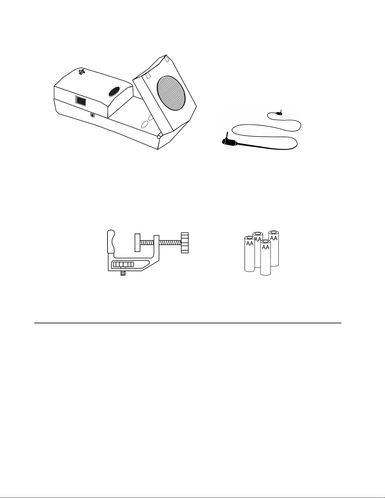
Calculator-Based Rangeré (CBRé) calculator-to-CBR cable

clamp 4 AA batteries

Important notice regarding book materials

Texas Instruments makes no warranty, either expressed or implied, including but not limited to any implied warranties of merchantability and fitness for a particular purpose, regarding any programs or book materials and makes such materials available solely on an “as-is” basis.

In no event shall Texas Instruments be liable to anyone for special, collateral, incidental, or consequential damages in connection with or arising out of the purchase or use of these materials, and the sole and exclusive liability of Texas Instruments, regardless of the form of action, shall not exceed the purchase price of this book. Moreover, Texas Instruments shall not be liable for any claim of any kind whatsoever against the use of these materials by any other party.

Permission is hereby granted to teachers to reprint or photocopy in classroom, workshop, or seminar quantities the pages or sheets in this work that carry a Texas Instruments copyright notice. These pages are designed to be reproduced by teachers for use in their classes, workshops, or seminars, provided each copy made shows the copyright notice. Such copies may not be sold and further distribution is expressly prohibited. Except as authorized above, prior written permission must be obtained from Texas Instruments Incorporated to reproduce or transmit this work or portions thereof in any other form or by any other electronic or mechanical means, including any information storage or retrieval system, unless expressly permitted by federal copyright law. Address inquiries to Texas Instruments Incorporated, PO Box 149149, Austin, TX, 78714-9149, M/S 2151, Attention: Contracts Manager.

Table of contents

CBR

)

NTRODUCTION

What is CBR? 2

Getting started with CBR — It’s as easy as 1, 2, 3 4

Hints for effective data collection 6

Activities with teacher notes and student activity sheets

TRIGGER

85-86

Activity 1 — Match the graph linear 13

Activity 2 — Toy car linear 17

Activity 3 — Pendulum sinusoidal 21

Activity 4 — Bouncing ball parabolic 25

Activity 5 — Rolling ball parabolic 29

Teacher information 33

Technical information

CBR data is stored in lists 37

RANGER settings 38 Using CBR with CBL or with CBL programs 39 Programming commands 40

Service information

Batteries 42

In case of difficulty 43

TI service and warranty 44

RANGER menu map inside back cover

OPYING PERMITTED PROVIDED

EXAS INSTRUMENTS INCORPORATED

ETTING STARTED WITH

CBR

What is CBR?

bring real-world data collection and analysis into the classroom

MATCH and BOUNCING BALL programs are built into RANGER

What does CBR do?

With

CBR

without tedious measurements and manual plotting.

lets students explore the mathematical and scientific relationships between distance,

CBR

velocity, acceleration, and time using data collected from activities they perform. Students can explore math and science concepts such as:

CBRCBRé ((Calculator-Based RangerCalculator-Based Rangeré

))

sonic motion detector

use with TI-82, TI-83, TI-85/

CBL

, TI-86, and TI-92

easy-to-use, self-contained

no programming required

Includes the RANGER programIncludes the RANGER program

the versatile RANGER program is one button away

primary sampling parameters are easy to set

and a TI graphing calculator, students can collect, view, and analyze motion data

motion: distance, velocity, acceleration

graphing: coordinate axes, slope, intercepts

functions: linear, quadratic, exponential, sinusoidal

calculus: derivatives, integrals

statistics and data analysis: data collection methods, statistical analysis

What’s in this guide?

Getting Started with CBR

calculator or programming experience. It includes quick-start instructions for using on effective data collection, and five classroom activities to explore basic functions and properties of motion. The activities (see pages 13–32) include:

teacher notes for each activity, plus general teacher information

step-by-step instructions

a basic data collection activity appropriate for all levels

explorations that examine the data more closely, including what-if scenarios

suggestions for advanced topics appropriate for precalculus and calculus students

a reproducible student activity sheet with open-ended questions appropriate for a wide

range of grade levels

is designed to be a guide for teachers who don’t have extensive

CBR

, hints

ETTING STARTED WITH

CBR

OPYING PERMITTED PROVIDED

EXAS INSTRUMENTS INCORPORATED

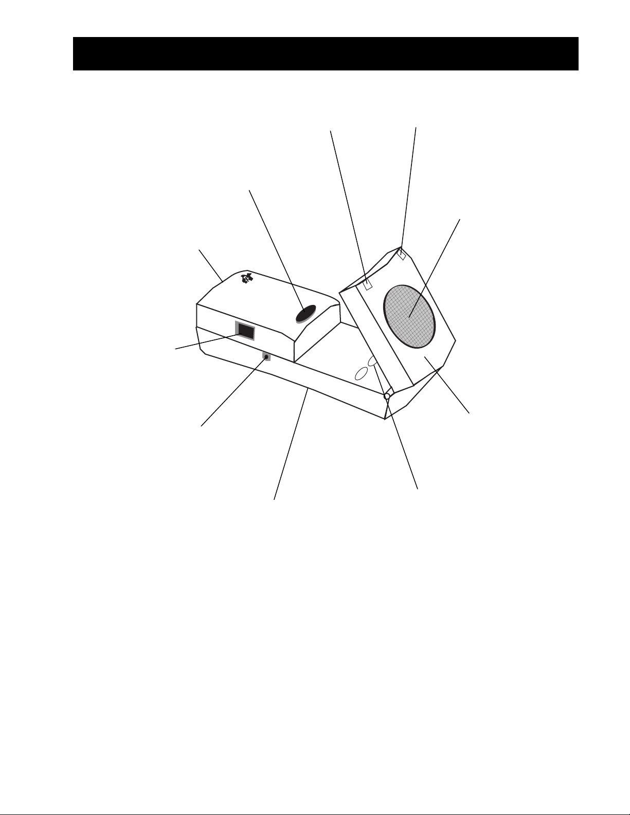
What is CBR?

(cont.)

to initiate sampling

battery door (on bottom)

port to connect to CBL (if desired)

port to connect to TI graphing calculators using the included

2.25-meter (7.5-foot) cable

reen light to indicate when data collection is occurring (sound also available)

button

CBR

)

red light to indicate

pecial conditions

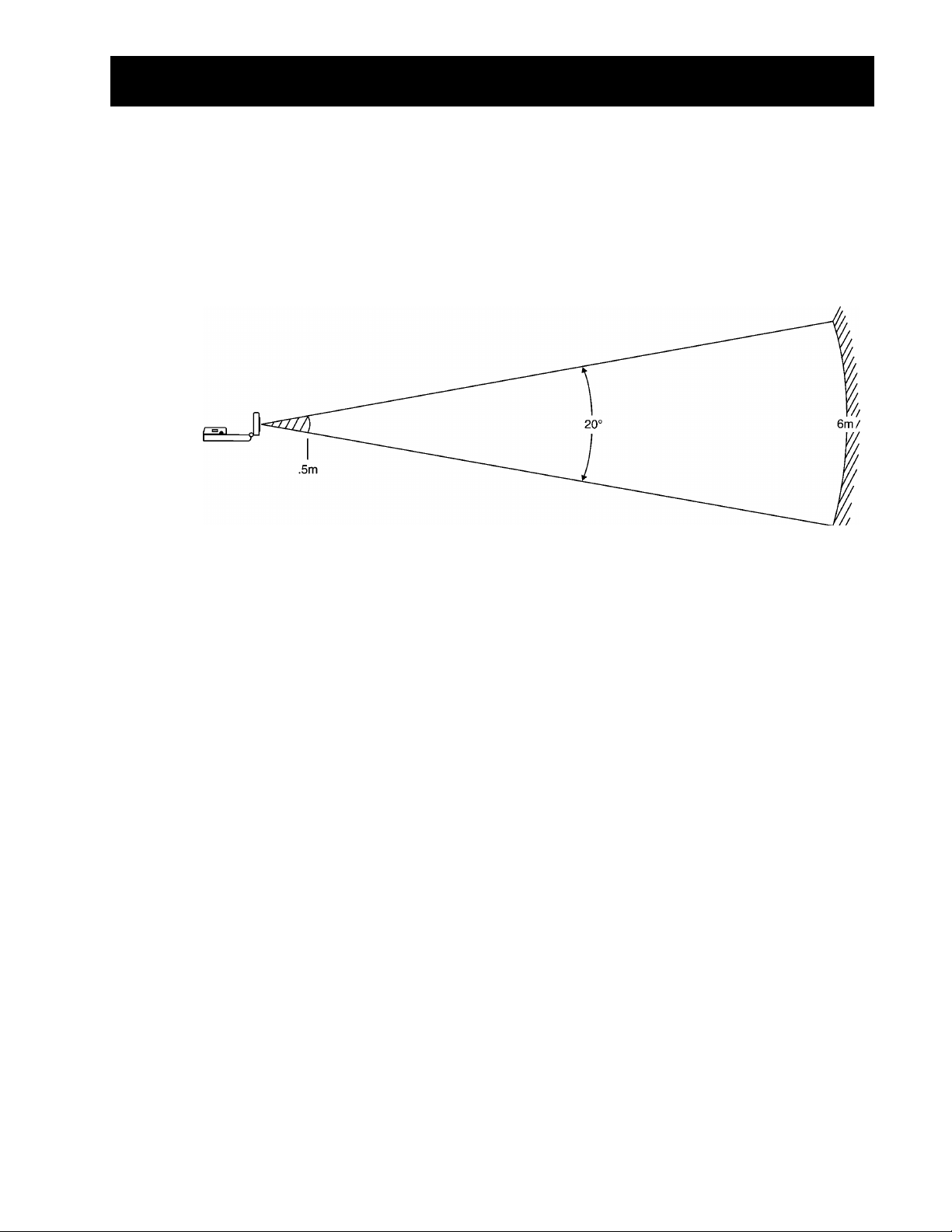
onic sensor to record up to 200 samples per second with a range between

0.5 meters and 6 meters (1.5 feet and 18 feet)

TRIGGER

85-86

pivoting head to aim

ensor accurately

tandard threaded socket to attach a tripod or the included mounting clamp

buttons to transfer RANGER program to calculators

(on back)

includes everything you need to begin classroom activities easily and quickly — just add

CBR

TI graphing calculators (and readily available props for some activities).

sonic motion detector

RANGER

OPYING PERMITTED PROVIDED

program in the

EXAS INSTRUMENTS INCORPORATED

CBR

calculator-to-

4 AA batteries

CBR

cable

mounting clamp

5 fun classroom activities

ETTING STARTED WITH

CBR

Getting started with CBR—It’s as easy as 1, 2, 3

With

, you’re just three simple steps from the first data sample!

CBR

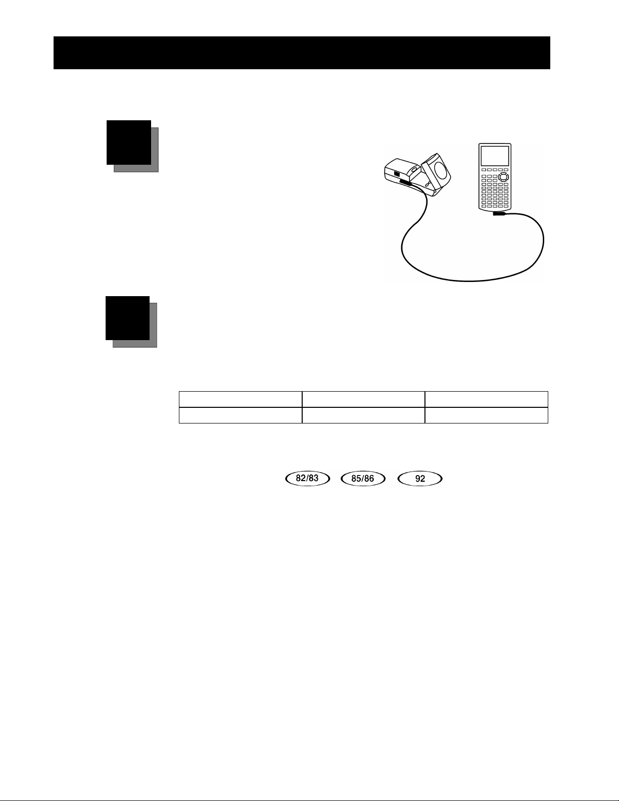
Connect

Connect using the calculator-to-

Push in connection.

The short calculator-to-calculator

Note:

cable that comes with the calculator also works.

to a TI graphing calculator

CBR

cable.

CBR

firmly

at both ends to make the

Transfer

RANGER

transfer the appropriate program from the

First, prepare the calculator to receive the program (see keystrokes below).

, a customized program for each calculator, is in the

to a calculator.

CBR

. It’s easy to

CBR

TI-82 or TI-83 TI-85/CBL or TI-86 TI-92

LINK

[

Next, open the pivoting head on the program-transfer button on the

During transfer, the calculator displays transfer is complete, the green light on and the calculator screen displays on

Once you’ve transferred the won’t need to transfer it to that calculator again unless you delete it from the calculator’s memory.

Note:

You may need to delete programs and data from the calculator. You can save the programs and data first by transferring them to a computer using TI-Graph Linké or to another calculator using a calculator-to-calculator cable or the calculator-to-

flashes twice and

CBR

The program and data require approximately 17,500 bytes of memory.

›

]

beeps twice.

CBR

RANGER

cable (see calculator guidebook).

CBR

LINK

CBR

DONE

[

]

, and then press the appropriate

CBR

RECEIVING

CBR

. If there is a problem, the red light

program from

Go to the Home screen.

(except TI-92). When the

flashes once,

CBR

beeps once,

CBR

to a calculator, you

ETTING STARTED WITH

CBR

OPYING PERMITTED PROVIDED

EXAS INSTRUMENTS INCORPORATED

Getting started with CBR—It’s as easy as 1, 2, 3

(cont.)

Run

Run the

RANGER

program (see keystrokes below).

For quick results, try one of the classroomready activities in this guide!

TI-82 or TI-83 TI-85/

Press Choose Press

RANGER

›

^ A

Press Choose

›

Press

or TI-86 TI-92

CBL

RANGER

Press L [ Choose Press ¨

VAR-LINK

RANGER

›

The opening screen is displayed.

Press

›. The

MAIN MENU

SETUPàSAMPLE SET DEFAULTS APPLICATIONS PLOT MENU TOOLS QUIT

From the Press

MAIN MENU

› to choose

MAIN MENU

& & & & &

choose

is displayed.

view/change the settings before sampling change the settings to the default settings

DISTANCE MATCH, VELOCITY MATCH, BALL BOUNCE

plot options

GET CBR DATA, GET CALC DATA, STATUS, STOPàCLEAR

SET DEFAULTS

START NOW

. The

. Set up the activity, and then press › to

screen is displayed.

SETUP

begin data collection. It’s that easy!

Important information

This guide applies to all TI graphing calculators that can be used with so you may find that some of the menu names do not match exactly those on your calculator.

When setting up activities, ensure that the

is securely anchored and

CBR

that the cord cannot be tripped over.

Always exit the

RANGER

program performs a proper shutdown of ensures that

Always disconnect

is properly initialized for the next time you use it.

CBR

program using the

CBR

from the calculator before storing it.

CBR

option. The

QUIT

when you choose

RANGER

QUIT

]

CBR

. This

OPYING PERMITTED PROVIDED

EXAS INSTRUMENTS INCORPORATED

ETTING STARTED WITH

CBR

Hints for effective data collection

Getting better samples

How does CBR work?

Understanding how a sonic motion detector works can help you get better data plots. The motion detector sends out an ultrasonic pulse and then measures how long it takes for that pulse to return after bouncing off the closest object.

, like any sonic motion detector, measures the time interval between transmitting the

CBR

ultrasonic pulse and the first returned echo, but

much more. When the data is collected,

using a speed-of-sound calculation. Then it computes the first and second derivatives of

CBR

the distance data with respect to time to obtain velocity and acceleration data. It stores these measurements in lists

L1, L2, L3

, and L4.

calculates the distance of the object from the

CBR

has a built-in microprocessor that does

CBR

Performing the same calculations as

Collect sample data in

➊

Use the sample times in

➋

REALTIME=NO

in conjunction with the distance data in L2 to calculate the

is an interesting classroom activity.

CBR

mode. Exit the

RANGER

program.

velocity of the object at each sample time. Then compare the results to the velocity data in

(

Use the velocity data in L3 (or the student-calculated values) in conjunction with the

➌

sample times in

n+1

to calculate the acceleration of the object at each sample time. Then

)à2 N (

n+1

compare the results to the acceleration data in

Object size

Using a small object at a far distance from the

decreases the chances of an accurate

CBR

n-1

)à2

reading. For example, at 5 meters, you are much more likely to detect a soccer ball than a ping-pong ball.

Minimum range

When the

the

CBR.

be misidentified by

sends out a pulse, the pulse hits the object, bounces back, and is received by

CBR

If an object is closer than 0.5 meters (1.5 feet), consecutive pulses may overlap and

. The plot would be inaccurate, so position

CBR

at least 0.5 meters

CBR

away from the object.

Maximum range

As the pulse travels through the air, it loses its strength. After about 12 meters (6 meters on the trip to the object and 6 meters on the trip back to the weak to be reliably detected by the the

ETTING STARTED WITH

. This limits the typical reliably effective distance from

CBR

to the object to less than 6 meters (19 feet).

CBR

), the return echo may be too

CBR

OPYING PERMITTED PROVIDED

EXAS INSTRUMENTS INCORPORATED

Hints for effective data collection

The clear zone

(cont.)

The path of the

beam is not a narrow, pencil-like beam, but fans out in all directions up

CBR

to 10° in a cone-shaped beam.

To avoid interference from other objects in the vicinity, try to establish a clear zone in the path of the recorded by

Reflective surfaces

beam. This helps ensure that objects other than the target do not get

CBR

CBR. CBR

records the closest object in the clear zone.

Some surfaces reflect pulses better than others. For example, you might see better results with a relatively hard, smooth surfaced ball than with a tennis ball. Conversely, samples taken in a room filled with hard, reflective surfaces are more likely to show stray data points. Measurements of irregular surfaces (such as a toy car or a student holding a calculator while walking) may appear uneven.

A Distance-Time plot of a nonmoving object may have small differences in the calculated distance values. If any of these values map to a different pixel, the expected flat line may show occasional blips. The Velocity-Time plot may appear even more jagged, because the change in distance between any two points over time is, by definition, velocity. You may wish to apply an appropriate degree of smoothing to the data.

OPYING PERMITTED PROVIDED

EXAS INSTRUMENTS INCORPORATED

ETTING STARTED WITH

CBR

Hints for effective data collection

RANGER settings

Sample times

is the total time in seconds to complete all sampling. Enter an integer between 1

TIME

second (for fast moving objects) and 99 seconds (for slow moving objects). For

REALTIME=YES, TIME

is always 15 seconds.

(cont.)

When

TIME=1 SECOND

Starting and stopping

The

SETUP

is a lower number, the object must be closer to the

TIME

, the object can be no more than 1.75 meters (5.5 feet) from the

screen in the

RANGER

program provides several options for starting and stopping

. For example, when

CBR

sampling.

BEGIN ON: [ENTER]

. Starts sampling with the calculator’s

key when the person

›

initiating the sampling is closest to the calculator.

BEGIN ON: [TRIGGER]

. Starts and stops sampling with the

person initiating the sampling is closest to the In this option, you also can choose to detach the

disconnect the cord from the sample, reattach the

, and press

CBR

, take the

CBR

to transfer the data. Use

›

CBR

. This lets you set up the sample,

CBR

where the action is, press

CBR

button when the

BEGIN ON: [TRIGGER]

when the cord is not long enough or would interfere with data collection. This is not available in

BEGIN ON: DELAY

REALTIME=YES

. Starts sampling after a 10-second delay from the time you press

mode (such as the

MATCH

application).

It is especially useful when only one person is doing an activity.

Trigger button

The effect of

varies depending on the settings.

CBR

›

ETTING STARTED WITH

starts sampling, even if

BEGIN ON: [ENTER]

BEGIN ON: DELAY

is selected. It also

stops sampling, but usually you will want to let a sample complete. In

REALTIME=NO

, after sampling has stopped,

automatically repeats the most recent sample, but does not transfer the data to the calculator. To transfer this data, from the

MAIN MENU

sample by choosing

choose

TOOLS

REPEAT SAMPLE

, and then choose

from the

PLOT MENU

GET CBR DATA

START NOW

. (You also can repeat a

from the

SETUP

screen.)

CBR

OPYING PERMITTED PROVIDED

EXAS INSTRUMENTS INCORPORATED

Hints for effective data collection

Smoothing

(cont.)

Smoothing capabilities built into the

RANGER

program can reduce the effect of stray signals or variations in the distance measurements. Avoid excessive smoothing. Begin with no smoothing or

smoothing. Increase the degree of smoothing until you obtain

LIGHT

satisfactory results.

For an activity with a higher-than-average likelihood of stray signals, you may wish to

increase the smoothing on the For already-collected

REALTIME=NO

calculator must be connected to the choose

Noise—what is it and how do you get rid of it?

When the

SMOOTH DATA

receives signals reflected from objects other than the primary target, the plot

CBR

, and then choose the degree of smoothing.

screen before sampling (see page 38).

SETUP

data, you can apply smoothing to the data. The

. Choose

CBR

PLOT TOOLS

from the

PLOT MENU

shows erratic data points (noise spikes) that do not conform to the general pattern of the plot. To minimize noise:

Make sure the

viewing a

REALTIME=NO

Try to sample in a clutter-free space (see the clear zone drawing on page 7).

Choose a larger, more reflective object or move the object closer to the

REALTIME=YES

is pointed directly at the target. Try adjusting the sensor head while

CBR

sample until you get good results before collecting a

sample.

CBR

(but farther

than 0.5 meters). When using more than one

in a room, one group should complete a sample before

CBR

the next group begins their sample. For a noisy

REALTIME=YES

obtain satisfactory results. (You cannot change the smoothing in the

VELOCITY MATCH

For a noisy

, or

REALTIME=NO

sample, repeat using a higher degree of smoothing until you

DISTANCE MATCH

BALL BOUNCE

applications.)

sample, you can apply a higher degree of smoothing to the

original data.

Speed of sound

The approximate distance to the object is calculated by assuming a nominal speed of sound. However, actual speed of sound varies with several factors, most notably the air temperature. For relative-motion activities, this factor is not important. For activities requiring highly accurate measurements, a programming command can be used to specify the ambient temperature (see pages 40–41).

OPYING PERMITTED PROVIDED

EXAS INSTRUMENTS INCORPORATED

ETTING STARTED WITH

CBR

Hints for effective data collection

REALTIME=YES

(cont.)

Use

REALTIME=YES

for slower objects

to see the results as they are collected

when you need to collect or plot only one type of data (distance, velocity, or acceleration)

mode:

for a sample

REALTIME=YES

mode, the

processes the requested plot data (distance, velocity, or

CBR

acceleration), which is transferred to the calculator following each individual distance measurement. Then

RANGER

plots a single pixel for that pulse.

Because all of these operations must be completed before the next sample can be requested, the maximum rate at which data can be sampled in

REALTIME=YES

mode is

limited.

It takes approximately 0.080 seconds just to sample, process, and transfer the data for a single data point. Additional time is required for operations such as plotting the point, which slows the effective sample rate to approximately 0.125 seconds in

REALTIME=NO

Use

REALTIME=NO

for faster objects

when smoothing is required (see page 9)

to operate the

when you need to collect or plot all types of data (distance, velocity, and acceleration) for

mode:

in detached mode (see page 11)

CBR

RANGER

a sample

In after all sampling is completed. The sample rate can be as fast as once every 0.005 seconds for close objects. Data for time, distance, velocity, and acceleration is transferred to the calculator.

Because the data is stored in the

and again.

ETTING STARTED WITH

REALTIME=NO

mode, data is stored in the

, you can transfer it from the

CBR

Each time you change smoothing, the

CBR

and not transferred to the calculator until

CBR

to a calculator again

CBR

applies the new smoothing factor, transfers

the adjusted data to the calculator, and stores the smoothed values in the lists. Choosing a domain changes the lists stored in the calculator. If you need to, you can

recover the original data from the choose

TOOLS

. From the

menu, choose

TOOLS

. From the

CBR

MAIN MENU

GET CBR DATA

in the

RANGER

program,

You also can share the same data with many students, even if they are using different types of TI graphing calculators. This allows all students to participate in data analysis activities using the same data (see page 11).

CBR

OPYING PERMITTED PROVIDED

EXAS INSTRUMENTS INCORPORATED

Hints for effective data collection

Using CBR in detached mode

(cont.)

Because the settings are required. On the

The special procedures are required.

Sharing data

What if you want the entire class to analyze the same data at the same time? With can disseminate

➊ ➋ ➌

➍

➎

cannot send data to the calculator immediately in detached mode, certain

CBR

screen:

SETUP

Set

REALTIME=NO

Set

BEGIN ON=[TRIGGER]

RANGER

program prompts you when to detach the

Transfer the

Collect the data with the

REALTIME=NO

RANGER

program to all students’ calculators prior to data collection.

data quickly within a classroom.

CBR

REALTIME=NO

mode.

Have the first student attach his or her calculator to the to-

From the choose

Press › to return to the

cable or the calculator-to-calculator cable.

CBR

MAIN MENU

GET CBR DATA. TRANSFERRING...

in the

RANGER

PLOT MENU

program, choose

is displayed and the plot appears.

, and then choose

and when to reattach it. No

CBR

using either the calculator-

CBR

. From the

TOOLS

QUIT

. Detach the cable.

TOOLS

you

CBR

menu,

Connect another calculator (of the same type) to the calculator with the data. On the

➏

receiving calculator, from the the

menu, choose

TOOLS

MAIN MENU

GET CALC DATA

set the sending calculator. When it is ready, press

in the

RANGER

program, choose

. Instructions are displayed telling you how to

›, and lists

L1, L2, L3, L4

are transferred automatically.

Transfer the data to another student’s calculator from

➐

while other students

CBR

continue the calculator-to-calculator transfers.

Once all students have the same data, they can analyze the data in

or outside

RANGER

To share data on the TI-85, use the

using the calculator’s list and graphing features.

feature outside of

LINK

RANGER

to transfer the lists.

using the

TOOLS

, and

. From

PLOT

OPYING PERMITTED PROVIDED

EXAS INSTRUMENTS INCORPORATED

ETTING STARTED WITH

CBR

Hints for effective data collection

Beyond simple data collection

(cont.)

Once you’ve collected and plotted data in

RANGER

, you can explore the data in relationship to a function. Because the data is collected as lists and displayed as a statistical plot, you can use

, , and œ to explore this relationship.

Inside RANGER

Explore plots using

, which is set automatically. (On the TI-85, use the free-moving

TRACE

cursor.) Manipulate the data set, including smoothing the data or selecting the domain of

interest.

Outside RANGER

Explore data using the calculator’s list editor.

Manually model a function to the data using the calculator’s Y= editor.

Automatically determine the equation that best fits the data using the calculator’s

regression capabilities.

Other relationships can be explored beyond those represented by the plot options in

RANGER

as statistical plots. From the

Plot1

. For instance, simultaneous plots of Distance-Time and Velocity-Time can be viewed

as L1 versus L2 and

MAIN MENU

as L1 versus L3. (You may also need to adjust the Window.)

Plot2

in the

RANGER

program, choose

, and then set

QUIT

Data and plots can be sent to a computer using TI-Graph Link. This is especially useful when students generate more involved reports of their activity findings.

Using CBR without the RANGER program

You can use

For information on using

For information on obtaining programs and activities, see page 36.

For information on programming commands to write your own programs, see pages

as a sonic motion detector with

CBR

with

CBR

40–41.

, see page 39.

CBL

or with programs other than

CBL

RANGER

ETTING STARTED WITH

CBR

OPYING PERMITTED PROVIDED

EXAS INSTRUMENTS INCORPORATED

Activity 1—Match the graph notes for teachers

Concepts

Function explored: linear. MATCH introduces the real-world concepts of distance

and time—or more precisely, the concept of distance versus time. As students attempt to duplicate graphs by walking while seeing their motion plotted, the concept of position can be explored.

In Explorations, students are asked to convert their rate of walking in meters per second to kilometers per hours.

Once they have mastered the Distance-Time match, challenge your students to a Velocity-Time match.

Materials

Ÿ calculator Ÿ CBR Ÿ calculator-to-calculator cable

A TI ViewScreené allows other students to watch— and provides much of the fun of this activity.

Hints

Students really enjoy this activity. Plan adequate time because everybody will want to try it!

This activity works best when the student who is walking (and the entire class) can view his or her motion projected on a wall or screen using the TI ViewScreen.

Typical answers

1. time (from start of sample); seconds; 1 second; distance (from the CBR to the object); meters; 1 meter

2. the y-intercept represents the starting distance

3. varies by student

4. backward (increase the distance between the CBR and the object)

5. forward (decrease the distance between the CBR and the object)

6. stand still; zero slope requires no change in y (distance)

7. varies by graph; @yà3.3

8. varies by graph; @yà1

9. the segment with the greatest slope (positive or negative)

10. this is a trick question—the flat segment, because you don’t move at all!

11. walking speed; when to change direction and/or speed

12. speed (or velocity)

13. varies by graph (example: 1.5 meters in 3 seconds)

14. varies by graph; example: 0.5 metersà1 second

Guide the students to walk in-line with the CBR; they sometimes try to walk sideways (perpendicular to the line to the CBR) or even to jump up!

Instructions suggest that the activity be done in meters, which matches the questions on the student activity sheet.

See pages 6–12 for hints on effective data collection.

Typical plots

example: (0.5 meters à 1 second) Q (60 seconds à 1 minute) = 30 meters à minute

example: (30 meters à 1 minute) Q (60 minutes à 1 hour) = 1800 meters à hour

example: (1800 meters à 1 hour) Q (1 kilometer à 1000 meter) = .18 kilometers à hour.

Have students compare this last number to the velocity of a vehicle, say 96 kilometers à hour (60 miles per hour).

15. varies by graph; sum of the @y for each line segment.

OPYING PERMITTED PROVIDED

EXAS INSTRUMENTS INCORPORATED

ETTING STARTED WITH

CBR

Activity 1—Match the graph linear

Data collection

➊

Hold the

in one hand, and the calculator in the other. Aim the sensor directly at a

CBR

wall.

Hints:

The maximum distance of any graph is 4 meters (12 feet) from the minimum range is 0.5 meters (1.5 feet). Make sure that there is nothing in the clear zone (see page 7).

CBR

. The

Run the

➋ ➌ ➍

From the

RANGER

MAIN MENU

APPLICATIONS

displayed.

Press › to display the graph to match. Take a moment to study the graph. Answer

➎

program (see page 5 for keystrokes for each calculator).

choose

menu choose

DISTANCE MATCH

APPLICATIONS

automatically takes care of the settings.

. Choose

DISTANCE MATCH

METERS

. General instructions are

questions 1 and 2 on the activity sheet.

Position yourself where you think the graph begins. Press › to begin data collection.

➏

You can hear a clicking sound and see the green light as the data is collected.

Walk backward and forward, and try to match the graph. Your position is plotted on

➐

the screen.

When the sample is finished, examine how well your “walk” matched the graph, and

➑

then answer question 3.

Press › to display the

➒

OPTIONS

menu and choose

SAME MATCH

. Try to improve your

walking technique, and then answer questions 4, 5, and 6.

ETTING STARTED WITH

CBR

OPYING PERMITTED PROVIDED

EXAS INSTRUMENTS INCORPORATED

Activity 1—Match the graph

Explorations

(cont.)

linear

DISTANCE MATCH

Press › to display the

➊

segment and answer questions 7 and 8.

Study the entire graph and answer questions 9 and 10.

➋

Position yourself where you think the graph begins, press › to begin data collection,

➌

and try to match the graph.

When the sampling stops, answer questions 11 and 12.

➍

Press › to display the

➎

Study the graph and answer questions 13, 14, and 15.

➏

Press › to display the

➐

MAIN MENU

Advanced explorations

The graphs generated by in which you must match a Velocity-Time plot. This one’s tough!

MATCH

is a very popular program. Additional versions that explore more complicated graphs

may be available (see page 36).

, all graphs are comprised of three straight-line segments.

OPTIONS

, and then choose

DISTANCE MATCH

menu and choose

NEW MATCH

menu. Repeat the activity if desired, or return to the

to exit the

QUIT

RANGER

program.

were all straight lines. Now try

. Study the first

VELOCITY MATCH

OPYING PERMITTED PROVIDED

EXAS INSTRUMENTS INCORPORATED

ETTING STARTED WITH

CBR

Activity 1—Match the graph

Name ___________________________________

Data collection

What physical property is represented along the x-axis? _____________________________________

What are the units? How far apart are the tick marks? ________________

What physical property is represented along the y-axis? _____________________________________

What are the units? How far apart are the tick marks? ________________

How far from the

Did you begin too close, too far, or just right? _____________________________________________

Should you walk forward or backward for a segment that slopes up? _________________________

do you think you should stand to begin? ______________________________

CBR

Why? _______________________________________________________________________________

Should you walk forward or backward for a segment that slopes down? ______________________

Why? _______________________________________________________________________________

What should you do for a segment that is flat? ____________________________________________

Why? _______________________________________________________________________________

Explorations

If you take one step every second, how long should that step be? ____________________________

If, instead, you take steps of 1 meter (or 1 foot) in length, how many steps must you take? _______

For which segment will you have to move the fastest? ______________________________________

Why? _______________________________________________________________________________

For which segment will you have to move the slowest? _____________________________________

10.

Why? _______________________________________________________________________________

In addition to choosing whether to move forward or backward, what other factors entered into

11.

matching the graph exactly? ____________________________________________________________

____________________________________________________________________________________

What physical property does the slope, or steepness of the line segment, represent? ____________

12.

For the first line segment, how many meters must you walk in how many seconds? _____________

13.

Convert the value in question 13 (the velocity) to metersà1 second: ___________________________

14.

Convert to metersàminute: _____________________________________________________________

Convert to metersàhour: _______________________________________________________________

Convert to kilometersàhour: ____________________________________________________________

How far did you actually walk? _________________________________________________________

15.

ETTING STARTED WITH

CBR

OPYING PERMITTED PROVIDED

EXAS INSTRUMENTS INCORPORATED

Activity 2—Toy car notes for teachers

Concepts

Function explored: linear. The motion of a motorized toy car is used to illustrate

the real-world concept of constant velocity.

Materials

Ÿ calculator Ÿ CBR Ÿ calculator-to-CBR cable Ÿ battery-operated toy car Ÿ TI ViewScreen (optional)

Hints

Toy cars vary greatly in size, shape, and angle of reflection of the incident ultrasonic sound. Therefore, the resulting plots may vary in quality. Some vehicles may require an additional reflective surface in order to obtain good plots. Try mounting an index card to the vehicle to assure a good target for the sensor.

You may wish to try a variety of vehicles so the students can explore these effects.

Toy cars that are slower (such as those designed for younger children) are better for this activity. Look for a car that appears to keep a constant velocity.

See pages 6–12 for hints on effective data collection.

Explorations

The slope of an object’s Distance-Time plot at any time gives the object’s speed at that time. Thus, for an object traveling at constant velocity, the slope of its Distance-Time plot is constant. This is why the Distance-Time plot exhibits a linear relationship.

If you start collecting data before the car begins moving, you will notice the Distance-Time plot is not linear at the beginning of the plot. Why? The car begins at rest (v = 0). It cannot instantaneously attain its constant velocity. Acceleration is given by:

∆

In order for the object to go instantaneously from rest to its constant velocity, ∆t = 0. But this implies infinite acceleration, which is not physically possible. (In fact, by Newton’s Second Law, F = ma, an infinite acceleration could only result from an infinite force, which is equally impossible.) Thus we must observe the object accelerating (increasing its speed) to its constant velocity over a finite time period.

Typical plots

Answers to questions

1. the first or last plot; distance increases at constant rate

2. students enter values from TRACE

3. distance values increase by a constant amount

4. velocity is rate of change for distance over time; the values are the same for each equal time increment

5. student should get a value similar to the values calculated for m

similar to m m represents velocity or speed of car

6. b is the y-intercept; example: y = 2x + 0

7. varies; for example, if m = 2, distance (y) = 20 meters after 10 seconds (y = 2 Q 10 + 0); for 1 minute, y = 120 meters

Advanced Explorations

The slope of a Velocity-Time plot for constant velocity is zero. Therefore, the Acceleration-Time plot shows a = 0 (in the ideal case) over the time period where velocity is constant.

The resulting area is the object’s displacement (net distance traveled) during the time interval t

For calculus students, the displacement can be found from:

svdt

∫

where s is the object’s displacement in the interval t to t2.

to t2.

OPYING PERMITTED PROVIDED

EXAS INSTRUMENTS INCORPORATED

ETTING STARTED WITH

CBR

Activity 2—Toy car linear

Data collection

Position the car at least 0.5 meters (1.5 feet) from the

➊

, facing away from the

CBR

a straight line.

Hints:

Aim the sensor directly at the car and make sure that there is nothing in the

clear zone (see page 7).

Before starting data collection, answer question 1 on the activity sheet.

➋ ➌ ➍

Run the

From the

RANGER

MAIN MENU

program (see page 5 for keystrokes for each calculator).

choose

SETUPàSAMPLE

. For this activity, the settings should be:

CBR

REALTIME: NO

TIME (S): 5 SECONDS

DISPLAY: DISTANCE

BEGIN ON: [ENTER]

SMOOTHING: LIGHT

UNITS: METERS

Instructions for changing a setting are on page 38.

Choose

➎

Press › when you are ready to begin. Start the car and quickly move out of the clear

➏

START NOW

zone. You can hear a clicking sound as the data is collected and the message

TRANSFERRING...

When the data collection is concluded, the calculator automatically displays a Distance-

➐

is displayed on the calculator.

Time plot of the collected data points.

Compare the plot of the data results to your prediction in answer 1 for similarities and

➑

differences.

ETTING STARTED WITH

CBR

OPYING PERMITTED PROVIDED

EXAS INSTRUMENTS INCORPORATED

Activity 2—Toy car

Explorations

The values for x (time) in half-second intervals are in the first column in question 2.

➊

Trace the plot and enter the corresponding y (distance) values in the second column.

disregard inconsistent data at the beginning of the data collection. Also, you may need to approximate the distance (the calculator may give you distance for 0.957 and 1.01 seconds instead of exactly 1 second). Pick the closest one or take your best guess.

➋

Answer questions 3 and 4.

Calculate the changes in distance and time between each data point to complete the

➌

third and fourth columns. For example, to calculate @Distance (meters) for 1.5 seconds, subtract Distance at 1 second from Distance at 1.5 seconds.

The function illustrated by this activity is y = mx + b. m is the slope of a line. It is

➍

calculated by:

Include results only from the linear part of the plot. You may need to

Note:

(cont.) linear

The y-intercept represents b.

Calculate m for every point. Enter the values in the table in question 2.

➎

Answer questions 5, 6, and 7.

Advanced Explorations

Calculating the slope of a Distance-Time plot at any time gives the object’s approximate velocity at that time. Calculating the slope of a Velocity-Time plot gives the object’s approximate acceleration at that time. If velocity is constant, what does acceleration equal?

Predict what the Acceleration-Time plot for this Distance-Time plot looks like.

Find the area between the Velocity-Time plot and the x-axis between any two convenient times, t

and t2. This can be done by summing the areas of one or more rectangles, each

with an area given by:

What is the physical significance of the resulting area?

@distance

@time

distance

time

area = v∆t = v(t

N distance

N time

2Nt1

)

N y

x2 N x

OPYING PERMITTED PROVIDED

EXAS INSTRUMENTS INCORPORATED

ETTING STARTED WITH

CBR

Activity 2—Toy car

Name ___________________________________

Data collection

Which of these do you think will match the Distance-Time plot of the toy car?

Why?________________________________________________________________________________

Time Distance

1 xxx xxx xxx

1.5 2

2.5 3

3.5 4

4.5 5

What do you notice about the Distance values? ____________________________________________

How do these results show that the toy car had constant velocity? ____________________________

Calculate @

distanceà@time

Distance

Time

between Time = 2 and Time = 4. ________________________________

What did you notice about this result? ___________________________________________________

What do you think m represents? _______________________________________________________

For the linear equation y = mx + b, what is the value for b? _________________________________

Write the equation for the line in the y = mx + b form, using values for m and b. _______________

How far would the toy car travel in 10 seconds? ___________________________________________

In 1 minute? _________________________________________________________________________

ETTING STARTED WITH

CBR

OPYING PERMITTED PROVIDED

EXAS INSTRUMENTS INCORPORATED

Activity 3—Pendulum notes for teachers

Concepts

Function explored: sinusoidal. Explore simple harmonic motion by observing a free-

swinging pendulum.

Materials

Ÿ calculator Ÿ CBR Ÿ calculator-to-CBR cable Ÿ mounting clamp Ÿ stopwatch Ÿ pendulum Ÿ meter stick Ÿ TI ViewScreen (optional)

Ideas for weights:

balls of different sizes (≥ 2" diameter)

soda cans (empty and filled)

bean bags

Hints

See pages 6–12 for hints on effective data collection.

Physical connections

An object that undergoes periodic motion resulting from a restoring force proportional to its displacement from its equilibrium (rest) position is said to exhibit simple harmonic motion (SHM). SHM can be described by two quantities.

The period T is the time for one complete cycle.

The amplitude A is the maximum displacement of the object from its equilibrium position (the position of the weight when at rest).

For a simple pendulum, the period T is given by:

= 2p

where L is the string length and g is the magnitude of the acceleration due to gravity. T does not depend on the mass of the object or the amplitude of its motion (for small angles).

The frequency f (number of complete cycles per second) can be found from:

f =

, where f is in hertz (Hz) when T is in seconds.

The derivatives of a sinusoidal plot are also sinusoidal. Note particularly the phase relationship between the weight’s position and velocity.

Typical plots

Typical answers

1. varies (in meters)

2. varies (in meters)

3. varies (in seconds); T (one period) = total time of 10 periodsà10; averaging over a larger sample tends to minimize inherent measurement errors

4. the total arc length, which should be approximately 4 times the answer to question 2; because an arc is longer than a straight line

5. sinusoidal, repetitive, periodic; distance from the xaxis to the equilibrium position

6. each cycle is spread out horizontally; a plot spanning 10 seconds must fit more cycles in same amount of screen space, therefore cycles appear closer together

7. (total # of cycles)à(5 seconds) = cyclesàsecond; easier to view full cycles, and fewer measurement errors

8. f = 1àT, where T is time for 1 period

9. decreased period; increased period (Pendulum length is directly related to period time;

the longer the string, the longer the period. Students can explore this relationship using the calculator’s list editor, where they can calculate the period for various values of L.)

10. A (amplitude) = ¼ total distance that the pendulum travels in 1 period

11. both sinusoidal; differences are in amplitude and phase

12. equilibrium position

13. when position = maximum or minimum value (when the weight is at greatest distance from equilibrium).

14. It doesn’t. T depends only on L and g, not mass.

Advanced explorations

Data collection: the plot of L2 versus L3 forms an ellipse.

OPYING PERMITTED PROVIDED

EXAS INSTRUMENTS INCORPORATED

ETTING STARTED WITH

CBR

Activity 3—Pendulum sinusoidal

Data collection

Set up the pendulum. Align the pendulum so it swings in a direct line with the

➊

Hints:

Position the

at least 0.5 meters (1.5 feet) from the closest approach of the

CBR

weight. Make sure that there is nothing in the clear zone (see page 7).

amplitude

equilibrium position

Using a meter stick, measure the distance from the

➋

to the equilibrium position.

CBR

Answer question 1 on the activity sheet.

CBR

Measure how far you will you pull the weight away from the equilibrium position.

Answer question 2.

A pendulum cycle (a period) consists of one complete swing back and forth. Using a

➌

stopwatch, time ten full periods. Answer questions 3 and 4.

➍

Run the

RANGER

program (see page 5 for keystrokes for each calculator). An efficient

method is for one person start the pendulum while another operates the calculator and

. From the

CBR

Press › to display the settings. For this activity, they should be:

➎

REALTIME: NO

TIME (S): 10 SECONDS

DISPLAY: DISTANCE

BEGIN ON: [ENTER]

SMOOTHING: LIGHT

UNITS: METERS

Instructions for changing a setting are on page 38. When they are correct, choose

➏

START NOW

Press › when you are ready to begin. You can hear a clicking sound as the data is

➐

MAIN MENU

collected, and the message

choose

TRANSFERRING...

SETUPàSAMPLE

is displayed on the calculator.

➑

ETTING STARTED WITH

When the data collection is complete, the calculator automatically displays a DistanceTime plot of the collected data points. Answer question 5.

CBR

OPYING PERMITTED PROVIDED

EXAS INSTRUMENTS INCORPORATED

Activity 3—Pendulum

Explorations

Data collection 2

(cont.)

sinusoidal

From the

MAIN MENU

to 5 seconds. Repeat the data collection. Observe the plot. Answer questions 6 and 7.

The quantity you determined (cycles per second) is called the frequency. Although you calculated frequency in question 7 using the plot, you can find it mathematically from:

where T is the period in seconds, and f is the frequency in hertz (Hz).

f =

Answer question 8.

Data collections 3 and 4

Repeat the 5-second data collection two more times. First, shorten the string. Second, lengthen the string. After observing those plots, answer question 9.

Another important distance measurement affecting the motion of the pendulum is the

amplitude. The answer to question 2 was the amplitude of that pendulum swing. Answer question 10.

Advanced explorations

Data collection 5

From the

PLOT MENU

choose

SETUPàSAMPLE

VELOCITY-TIME

. On the

screen, change the time from 10

SETUP

. Answer questions 11, 12 and 13.

Data collection 6

Repeat the data collection with a significantly lighter or heavier weight, and then answer question 14.

Model the distance-time behavior of the pendulum using the form for a sinusoidal function,

S = A sin (wt +

frequency,

T, by w = 2

), where S is the instantaneous position, A is the amplitude, w is the

is the phase angle, and t is the time. The frequency, w, is related to the period,

pà

Enter this equation in the Y= editor using the calculated values of A and w. Simultaneously graph this function and the statistical plot of of A, w, and

until a good fit is obtained. On the TI-83 or TI-86, use the sine regression to

(time) versus L2 (distance). Adjust the values

determine the values.

Explore the relationship between position and velocity by plotting

(distance) versus

(velocity). What do you predict for the appearance of the resulting plot? Compare the actual result to your prediction.

OPYING PERMITTED PROVIDED

EXAS INSTRUMENTS INCORPORATED

ETTING STARTED WITH

CBR

Activity 3—Pendulum

Data collection

Name ___________________________________

What is the distance from

How far will you pull the pendulum away from the equilibrium position? ______________________

What was the time for ten periods? _____________________________________________________

to the equilibrium position? __________________________________

CBR

Calculate how long (in seconds) it took to complete one period. _____________________________

What is the benefit of timing ten complete periods instead of just one? _______________________

Use the answer to question 2, and approximate the total distance traveled in one cycle. _________

Why is this value shorter than the actual distance traveled in one cycle? _______________________

What do you notice about the shape of the plot? __________________________________________

How is the value from question 1 represented on the plot? __________________________________

Explorations

How does the appearance of the plot change? Why ? ______________________________________

____________________________________________________________________________________

Using data collected from your plot, calculate the number of complete cycles per second. ________

Why is it easier to determine this using the second plot (spanning 5 seconds) rather than the first one (spanning 10 seconds)?_____________________________________________________________

Calculate the frequency for one period using the equation. __________________________________

How does shortening the string length affect the period of the pendulum?_____________________

How does lengthening the string affect the period of the pendulum?

. What is the relationship between the amplitude of the pendulum swing and the total distance that

__________________________

the pendulum travels in one period? _____________________________________________________

____________________________________________________________________________________

Advanced explorations

Compare the Distance-Time plot with the Velocity-Time plot. List similarities and differences.______

11.

____________________________________________________________________________________

In what position is the weight’s velocity maximum? _________________________________________

12.

In what position is the weight’s velocity minimum? _________________________________________

13.

How does changing the weight affect the plot? Why? ______________________________________

14.

____________________________________________________________________________________

ETTING STARTED WITH

CBR

OPYING PERMITTED PROVIDED

EXAS INSTRUMENTS INCORPORATED

Activity 4—Bouncing ball notes for teachers

Concepts

Function explored: parabolic. Real-world concepts such as free-falling and bouncing

objects, gravity, and constant acceleration are examples of parabolic functions. This activity investigates the values of height, time, and the coefficient A in the quadratic equation,

Y = A(X – H)

+ K, which describes the behavior of a

bouncing ball.

Materials

Ÿ calculator Ÿ CBR Ÿ calculator-to-CBR cable Ÿ large (9-inch) playground ball Ÿ TI ViewScreen (optional)

Hints

This activity is best performed with two students, one to hold the ball and the other to push ¤.

See pages 6–12 for hints on effective data collection. The plot should look like a bouncing ball. If it does

CBR

not, repeat the sample, ensuring that the

is aimed

squarely at the ball. A large ball is recommended.

Typical plots

3. The Distance-Time plot for this activity does not

CBR

represent the distance from the

BALL BOUNCE

flips the distance data so the plot

to the ball.

better matches students’ perceptions of the ball’s behavior. y = 0 on the plot is actually the point at which the ball is farthest from the

CBR

, when the

ball hits the floor.

4. Students should realize that the x-axis represents time, not horizontal distance.

7. The graph for A = 1 is both inverted and broader than the plot.

8. A < L1

9. parabola concave up; concave down; linear

12. same; mathematically, the coefficient A represents the extent of curvature of the parabola; physically, A depends upon the acceleration due to gravity, which remains constant through all the bounces.

Advanced explorations

The rebound height of the ball (maximum height for a given bounce) is approximated by:

y = hp

y is the rebound height

h is the height from which the ball is released

p is a constant that depends on physical characteristics of the ball and the floor surface

x is the bounce number

, where

Explorations

After an object is released, it is acted upon only by gravity (neglecting air resistance). So A depends on the acceleration due to gravity, N9.8 metersàsecond

(N32 feetàsecond2). The negative sign indicates that the acceleration is downward.

The value for A is approximately one-half the acceleration due to gravity, or N4.9 metersàsecond

(N16 feetàsecond2).

Typical answers

1. time (from start of sample); seconds; height à distance of the ball above the floor; meters or feet

2. initial height of the ball above the floor (the peaks represent the maximum height of each bounce); the floor is represented by y = 0.

For a given ball and initial height, the rebound height decreases exponentially for each successive bounce. When x = 0, y = h, so the y-intercept represents the initial release height.

Ambitious students can find the coefficients in this equation using the collected data. Repeat the activity for different initial heights or with a different ball or floor surface.

After manually fitting the curve, students can use regression analysis to find the function that best models the data. Select a single bounce using

TOOLS

SELECT DOMAIN

. Then

QUIT

from the

PLOT

MAIN MENU

Follow the calculator operating procedures to perform a quadratic regression on lists

and L2.

Extensions

Integrate under Velocity-Time plot, giving the displacement (net distance traveled) for any chosen time interval. Note the displacement is zero for any full bounce (ball starts and finishes on floor).

OPYING PERMITTED PROVIDED

EXAS INSTRUMENTS INCORPORATED

ETTING STARTED WITH

CBR

Activity 4—Bouncing ball parabolic

Data collection

Begin with a test bounce. Drop the ball (do not throw it).

➊

Hints:

Position the

at least 0.5 meters (1.5 feet) above the height of the highest

CBR

bounce. Hold the sensor directly over the ball and make sure that there is nothing in the clear zone (see page 7).

Run the

➋

From the

➌

From the

➍

BALL BOUNCE

RANGER

MAIN MENU

APPLICATIONS

program (see page 5 for keystrokes for each calculator).

choose

APPLICATIONS

menu choose

. Choose

BALL BOUNCE

METERS

FEET

. General instructions are displayed.

automatically takes care of the settings.

➎

➏

➐

➑

ETTING STARTED WITH

Hold the ball with arms extended. Press ›. The mode. At this point, you may detach

from the calculator.

CBR

RANGER

program is now in Trigger

Press ¤. When the green light begins flashing, release the ball, and then step back. (If the ball bounces to the side, move to keep the be careful

to change the height of the

not

CBR

directly above the ball, but

CBR

You can hear a clicking sound as the data is collected. Data is collected for time and distance, and calculated for velocity and acceleration. If you have detached the

CBR

reattach it when data collection is finished.

Press ›. (If the plot doesn’t look good, repeat the sample.) Study the plot. Answer

questions 1 and 2 on the activity sheet.

Observe that

BALL BOUNCE

automatically flipped the distance data. Answer

questions 3 and 4.

CBR

OPYING PERMITTED PROVIDED

EXAS INSTRUMENTS INCORPORATED

Activity 4—Bouncing ball

Explorations

The Distance-Time plot of the bounce forms a parabola.

(cont.)

parabolic

Press ›. From the

➊

want to select the first full bounce. Move the cursor to the base of the beginning of the bounce, and press then press

The plot is in

➋

the activity sheet.

Press › to return to the

➌

The vertex form of the quadratic equation, Y = A(X – H)

➍

analysis. Press vertex form of the quadratic equation: Yn=A…(X–H)^2+K.

On the Home screen, store the value you recorded in question 5 for the height in

➎

variable K; store the corresponding time in variable H; store 1 in variable A.

Press  to display the graph. Answer questions 6 and 7.

➏

Try A = 2, 0, –1. Complete the first part of the chart in question 8 and answer

➐

question 9.

Choose values of your own for A until you have a good match for the plot. Record

➑

your choices for A in the chart in question 8.

›. The plot is redrawn, focusing on a single bounce.

TRACE

œ. In the

PLOT MENU

›. Move the cursor to the base at the end of that bounce, and

mode. Determine the vertex of the bounce. Answer question 5 on

, choose

PLOT MENU

editor, turn off any functions that are selected. Enter the

PLOT TOOLS

. Choose

, and then

MAIN MENU

+ K, is appropriate for this

SELECT DOMAIN

. Choose

QUIT

. We

Repeat the activity, but this time choose the last (right-most) full bounce. Answer

➒

questions 10, 11, and 12.

Advanced explorations

Repeat the data collection, but do not choose a single parabola.

➊

Record the time and height for each successive bounce.

➋

Determine the ratio between the heights for each successive bounce.

➌

Explain the significance, if any, of this ratio.

➍

OPYING PERMITTED PROVIDED

EXAS INSTRUMENTS INCORPORATED

ETTING STARTED WITH

CBR

Activity 4—Bouncing ball

Name ___________________________________

Data collection

What physical property is represented along the x-axis? _____________________________________

What are the units? ___________________________________________________________________

What physical property is represented along the y-axis? _____________________________________

What are the units? ___________________________________________________________________

What does the highest point on the plot represent? ________________________________________

The lowest point? _____________________________________________________________________

Why did the

Why does the plot look like the ball bounced across the floor? _______________________________

BALL BOUNCE

program flip the plot? __________________________________________

Explorations

Record the maximum height and corresponding time for the first full bounce. __________________

Did the graph for A = 1 match your plot? _________________________________________________

Why or why not? _____________________________________________________________________

Complete the chart below.

A How do the data plot and the Yn graph compare?

What does a positive value for A imply? __________________________________________________

What does a negative value for A imply? _________________________________________________

What does a zero value for A imply? _____________________________________________________

Record the maximum height and corresponding time for the last full bounce. __________________

10.

Do you think A will be bigger or smaller for the last bounce? ________________________________

11.

How did A compare? __________________________________________________________________

12.

What do you think A might represent? ___________________________________________________

ETTING STARTED WITH

CBR

OPYING PERMITTED PROVIDED

EXAS INSTRUMENTS INCORPORATED

Activity 5—Rolling ball notes for teachers

Concepts

Function explored: parabolic. Plotting a ball rolling down a ramp of varying

inclines creates a family of curves, which can be modeled by a series of quadratic equations. This activity investigates the values of the coefficients in the quadratic equation, y = ax

+ bx + c.

Materials

Ÿ calculator Ÿ CBR Ÿ calculator-to-CBR cable Ÿ mounting clamp Ÿ large (9 inch) playground ball Ÿ long ramp (at least 2 meters or 6 feet—a

lightweight board works well)

Ÿ protractor to measure angles Ÿ books to prop up ramp Ÿ TI ViewScreen (optional)

Hints

Discuss how to measure the angle of the ramp. Let students get creative here. They might use a trigonometric calculation, folded paper, or a protractor.

See pages 6–12 for hints on effective data collection.

Typical plots

Typical answers

1. the third plot

2. time; seconds; distance of object from CBR; feet or meters

3. varies (should be half of a parabola, concave up)

4. a parabola (quadratic)

5. varies

6. varies (should be parabolic with increasing curvature)

7. 0¡ is flat (ball can’t roll); 90¡ is the same as a free-falling (dropping) ball

Explorations

The motion of a body acted upon only by gravity is a popular topic in a study of physical sciences. Such motion is typically expressed by a particular form of the quadratic equation,

s = ½at

0 0 0 0

In the quadratic equation y = ax y represents the distance from the

+ vit + si where

s is the position of an object at time t a is its acceleration vi is its initial velocity si is its initial position

+ bx + c,

CBR

to the ball at time x if the ball’s initial position was c, initial velocity was b, and acceleration is 2a.

Advanced explorations:

Since the ball is at rest when released, b should approach zero for each trial. c should approach the initial distance, 0.5 meters (1.5 feet). a increases as the angle of inclination increases.

If students model the equation y = ax manually, you may need to provide hints for the values of b and c. You may also direct them to perform a quadratic regression on lists their calculators. The ball’s acceleration is due to the earth’s gravity. So the more the ramp points down (the greater the angle of inclination), the greater the value of a. Maximum a occurs for q = 90¡, minimum for q = 0¡. In fact, a is proportional to the sine of q.

+ bx + c

L1, L2

using

OPYING PERMITTED PROVIDED

EXAS INSTRUMENTS INCORPORATED

ETTING STARTED WITH

CBR

Activity 5—Rolling ball parabolic

Data collection

➊

Answer question 1 on the activity sheet. Set the ramp at a 15° incline. Attach the clamp to the top edge of the ramp. Attach the and position it perpendicular to the ramp. Attach the calculator to the

to the clamp. Open the sensor head

CBR

Mark a spot on the ramp 0.5 meters (1.5 feet) from the ball at this mark, while a second student holds the calculator.

Hints:

Aim the sensor directly at the ball and make sure that there is nothing in the

clear zone (see page 7).

Run the

➋

Press › to display the settings. For this activity, they should be:

➌

SMOOTHING: LIGHT

RANGER

choose

REALTIME: NO

TIME (S): 3 SECONDS

DISPLAY: DISTANCE

BEGIN ON: [ENTER]

UNITS: METERS

program (see page 5 for keystrokes for each calculator). From the

SETUPàSAMPLE

. Have one student hold the

CBR

MAIN

➍ ➎ ➏

➐

ETTING STARTED WITH

Instructions for changing a setting are on page 38.

When the settings are correct, choose

START NOW

. Press › to begin sampling.

When the clicking begins, release the ball immediately (don’t push) and step back.

When the sample is complete, the Distance-Time plot is displayed automatically.

Answer questions 2 and 3.

Press › to display the

DOMAIN

. Move the cursor to where the ball was released, and then press ›. Move

PLOT MENU

the cursor to where the ball reached the end of the ramp, and then press

. Choose

PLOT TOOLS

, and then choose

›. The

SELECT

plot is redrawn, focusing on the portion of the sample that corresponds to the ball rolling down the ramp. Answer questions 4 and 5.

CBR

OPYING PERMITTED PROVIDED

EXAS INSTRUMENTS INCORPORATED

Activity 5—Rolling ball

Explorations

Examine what happens for differing inclines.

Predict what will happen if the incline increases. Answer question 6.

➊

Adjust the incline to 30¡. Repeat steps 2 through 6. Add this plot to the drawing in

➋

question 6, labeled 30¡.

Repeat steps 2 through 6 for inclines of 45¡ and 60¡ and add to the drawing.

➌ ➍

Answer question 7.

Advanced explorations

Adjust the time values so that x = 0 for the initial height (the time at which the ball was released. You can do this manually by subtracting the x value for the first point from all the points on your plot, or you can enter

(cont.)

L1(1)"A:L1NA"L1

parabolic

Calculate the values for a, b, and c for the family of curves in the form y = ax

➊

at 0¡, 15¡, 30¡, 45¡, 60¡, 90¡.

What are the minimum and maximum values for a? Why?

➋

Write an expression describing the mathematical relationship between a and the angle

➌

of inclination.

+ bx + c

OPYING PERMITTED PROVIDED

EXAS INSTRUMENTS INCORPORATED

ETTING STARTED WITH

CBR

Activity 5—Rolling ball

Name ___________________________________

Data collection

Which of these plots do you think best matches the Distance-Time plot of a ball rolling down a

ramp?

What physical property is represented along the x-axis? _____________________________________

What are the units? ___________________________________________________________________

What physical property is represented along the y-axis? _____________________________________

What are the units? ___________________________________________________________________

Sketch what the plot really looks like. Label the axis. Label the plot at the points when the ball was

released and when it reached the end of the ramp.

What type of function does this plot represent? ___________________________________________

Discuss your change in understanding between the graph you chose in question 1 and the curve

you sketched in question 3. ____________________________________________________________

____________________________________________________________________________________

Explorations

Sketch what you think the plot will look like with a greater incline. (Label it prediction.)

Sketch and label the plots for 0¡ and 90¡:

ETTING STARTED WITH

CBR

OPYING PERMITTED PROVIDED

EXAS INSTRUMENTS INCORPORATED

Teacher information

How might your classes change with CBR?

is an easy-to-use system with features that help you integrate it into your lesson plans

CBR

quickly and easily.

offers significant improvements over other data-collection methods you may have used

CBR

in the past. This, in turn, may lead to a restructuring of how you use class time, as your students become more enthusiastic about using real-world data.

You’ll find that your students feel a greater sense of ownership of the data because they

actually participate in the data-collection process rather than using data from textbooks, periodicals, or statistical abstracts. This impresses upon them that the concepts you explore in class are connected to the real world and aren’t just abstract ideas. But it also means that each student will want to take his or her turn at collecting the data.

Data collection with

is considerably more effective than creating scenarios and

CBR

manually taking measurements with a ruler and stopwatch. Since more sampling points give greater resolution and since a sonic motion detector is highly accurate, the shape of curves is more readily apparent. You will need less time for data collection and have more time for analysis and exploration.

With

students can explore the repeatability of observations and variations in what-if

CBR

scenarios. Such questions as “Is it the same parabola if we drop the ball from a greater height?” and “Is the parabola the same for the first bounce as the last bounce?” become natural and valuable extensions.

The power of visualization lets students quickly associate the plotted list data with the

physical properties and mathematical functions the data describes.

Other changes occur once the data from real-world events is collected.

lets your

CBR

students explore underlying relationships both numerically and graphically.

Explore data graphically

Use automatically generated plots of distance, velocity, and acceleration with respect to time for explorations such as:

What is the physical significance of the y-intercept? the x-intercept? the slope? the

maximum? the minimum? the derivatives? the integrals?

How do we recognize the function (linear, parabolic, etc.) represented by the plot?

How would we model the data with a representative function? What is the significance of

the various coefficients in the function (e.g., AX

Explore data numerically

Your students can employ statistical methods (mean, median, mode, standard deviation, etc.) appropriate for their level to explore the numeric data. When you exit the program, a prompt reminds you of the lists in which velocity, and acceleration is stored.

OPYING PERMITTED PROVIDED

EXAS INSTRUMENTS INCORPORATED

+ BX + C)?

RANGER

REALTIME=NO

data for time, distance,

ETTING STARTED WITH

CBR

Teacher information

(cont.)

CBR plots—connecting the physical world and mathematics

The plots created from the data collected by

RANGER

are a visual representation of the relationships between the physical and mathematical descriptions of motion. Students should be encouraged to recognize, analyze, and discuss the shape of the plot in both physical and mathematical terms. Additional dialog and discoveries are possible when functions are entered in the Y= editor and displayed with the data plots.

A Distance-Time plot represents the approximate position of an object (distance from the

) at each instant in time when a sample is collected. y-axis units are meters or feet;

CBR

x-axis units are seconds.

A Velocity-Time plot represents the approximate speed of an object (relative to, and in the

direction of, the

) at each sample time. y-axis units are metersàsecond or feetàsecond;

CBR

x-axis units are seconds.

An Acceleration-Time plot represents the approximate rate of change in speed of an

object (relative to, and in the direction of, the metersàsecond

The first derivative (instantaneous slope) at any point on the Distance-Time plot is the

or feetàsecond2; x-axis units are seconds.

) at each sample time. y-axis units are

CBR

speed at that instant.

The first derivative (instantaneous slope) at any point on the Velocity-Time plot is the

acceleration at that instant. This is also the second derivative at any point on the DistanceTime plot.

A definite integral (area between the plot and the x-axis between any two points) on the

Velocity-Time plot equals the displacement (net distance traveled) by the object during that time interval.

Speed and velocity are often used interchangeably. They are different, though related, properties. Speed is a scalar quantity; it has magnitude but no specified direction, as in “6 feet per second.” Velocity is a vector quantity; it has a specified direction as well as magnitude, as in “6 feet per second due North.”

A typical

Velocity-Time plot actually represents speed, not velocity. Only the

CBR

magnitude (which can be positive, negative, or zero) is given. Direction is only implied. A positive velocity value indicates movement away from the movement toward the

measures distance only along a line from the detector. Thus, if an object is moving at

CBR

; a negative value indicates

CBR

an angle to the line, it only computes the component of velocity parallel to this line. For example, an object moving perpendicular to the line from the

shows zero velocity.

CBR

ETTING STARTED WITH

CBR

OPYING PERMITTED PROVIDED

EXAS INSTRUMENTS INCORPORATED

Teacher information

(cont.)

The mathematics of distance, velocity, and acceleration

average

instantaneous

N d

lim

@t"

= slope of Distance-Time plot

N t

(

d(s)

)

Distance-Time plot

where s = distance

Velocity-Time plot

N v

average

instantaneous

lim

= slope of Velocity-Time plot

N t

(

)

The area under the Velocity-Time plot from t1 to t2 = @d = (d t

to t2 (net distance traveled).

t=2

⌠

⌡

t=1

v(dt)

So, @d =

(

t=2

∑

t=1

v(@t)

or @d =

)

Acceleration-Time plot

) = displacement from

2Nd1

OPYING PERMITTED PROVIDED

EXAS INSTRUMENTS INCORPORATED

ETTING STARTED WITH

CBR

Teacher information

Web-site resources

(cont.)

At our web site,

a listing of supplemental material for use with

a library of programs for use with

an activities page with applications developed and shared by teachers like you

programs that access additional

CBR

more detailed information about

Additional resources

Texas Instruments’ Explorations books provide supplemental material related to TI graphing calculators, including books with classroom activities for and high-school math and science classes.

http:ààwww.ti.comàcalc

CBR, CBL

CBR

settings and programming commands

CBR

, you’ll find:

CBR, CBL

, and TI graphing calculators

features

appropriate for middle-school

CBR

ETTING STARTED WITH

CBR

OPYING PERMITTED PROVIDED

EXAS INSTRUMENTS INCORPORATED

CBR data is stored in lists

Collected data is stored lists L1, L2, L3, and L4

When

collects data, it automatically transfers it to the calculator and stores the data in

CBR

lists. Each time you exit the

contains time data.

contains distance data.

contains velocity data.

contains acceleration data.

For example, the 5th element in list collected, and the 5th element in list

REALTIME=YES

, only the data for the requested plot (distance, velocity, or acceleration) is

calculated and transferred. In

Settings are stored in list L5

The

RANGER SETUP

screen makes it easy to change the most commonly-used

(see page 38).

When you transfer the new list containing the defaults.

See pages 40–41 for information about programming commands that change other settings.

RANGER

program, you are reminded of where the data is stored.

represents the time when the 5th data point was

represents the distance of the 5th data point.

REALTIME=NO

program from the

, all the data is calculated and transferred.

CBR

CBR, L5

is automatically replaced with a

parameters

Using the data lists

The lists are not deleted when you exit the additional graphical, statistical, and numerical explorations and analyses.

You can plot the lists against each other, display them in the list editor, use regression analysis, and perform other analytical activities. For example, you could collect the data from pendulum motion using explore elliptical functions. (You may also need to adjust the Window.)

RANGER

, exit

RANGER

program. Thus, they are available for

, and then plot Velocity-Acceleration to

OPYING PERMITTED PROVIDED

EXAS INSTRUMENTS INCORPORATED

ETTING STARTED WITH

CBR

RANGER settings

Changing RANGER settings

RANGER

➊

displays the most commonly used settings before data collection begins.

From the

MAIN MENU

in the

RANGER

program, choose

SETUPàSAMPLE

settings are shown. 4 indicates the location of the cursor.

MAIN MENU

REALTIME: & YES

TIME (S):

DISPLAY: & DISTANCE, VELOCITY

BEGIN ON:

SMOOTHING:

Press c or b to move to the setting you want to change.

➋

Press

➌

›

to move to the next option. To change

When all the settings are correct, press c or b until the cursor is on

➍

To continue, press

To return to the

The new settings remain unless you choose

program that changes the settings. If you manipulate

delete

, the default settings may be restored the next time you run

START NOW

UNITS:

& TOTAL TIME

= 1–99

& [ENTER], [TRIGGER], & NONE & METERS

LIGHT, MEDIUM

FEET

SECONDS

, or

ACCELERATION

10-SECOND DELAY

, or

HEAVY

(

to cycle through the available options. When the option is correct, press

, enter 1 or 2 digits, and then press c or

TIME

›

MAIN MENU

, press e, and then press

SET DEFAULTS

›

, run an application, or run another

outside the

. The current

REALTIME=NO

START NOW

RANGER

)

only

program or

Restoring RANGER settings to the defaults

The default settings are appropriate for a wide variety of sampling situations. If you are unsure of the best settings, begin with the default settings, and then adjust.

➊

From the

MAIN MENU

in the

RANGER

The settings are changed to the defaults and the

If you wish to change a setting from the default, follow the steps above.

➋

To continue, press

➌

when cursor is on

›

Other RANGER settings

The

RANGER

program accesses the most commonly changed settings. settings. See pages 40–41 for information about programming commands that change these settings.

program, choose

SETUP

START NOW

SET DEFAULTS

screen is displayed.

has additional

CBR

ETTING STARTED WITH

CBR

OPYING PERMITTED PROVIDED

EXAS INSTRUMENTS INCORPORATED

Using CBR with CBL or with CBL programs

Using CBR as a conventional motion detector with CBL

The

can be used as a conventional motion detector with the Texas Instruments

CBR

(Calculator-Based Laboratoryé) system.

Do not connect

CBR

calculator must be connected to

You may need to change the function with

CBL

at the same time that

CBL

Using CBR with programs written for CBL

A special cable is required to connect the

CBR

You may order the cable by calling 1-800-TI-CARES.

is connected to a calculator. The

CBR

program as noted below. The

CBL

RANGER

CBL

program does not

You can use

with most

CBR

programs written for only a motion detector with no

CBL

changes or only minor changes to the program.

To stop sampling:

With some

programs using

CBL

REALTIME=YES

data collection,

CBR

continues to sample indefinitely. To stop data collection at the end of the sample time, you can do either of the following:

Press ¤ on the

Add statements to the existing

CBR

program to send the command {6,0} to the

CBL

CBR

. The

statement must be at a point after the data is transferred and displayed. For example:

{6,0}"L6:SEND L6

To turn sound off or on:

To turn off the sound, add statements to the existing

program to send the command {6,3} to the

. The statement must be at a point before

CBR

CBL

data collection begins. For example:

{6,3}"L6:SEND L6

To turn on the sound, simply run the

In case of difficulty:

locked up, run the

If you run a

RANGER

an updated version of the

program. Check the TI web site (see page 36), which may have

CBL

program.

RANGER

program and

program.

CBR

appears to be unresponsive or

OPYING PERMITTED PROVIDED

EXAS INSTRUMENTS INCORPORATED

ETTING STARTED WITH

CBR

Programming commands

Command 0 Clears and resets system {0}

Clears all. Resets power-on defaults. Channel 11 automatically selected.

Command 1 Clears channels {1,0}

Clears channel settings; does not clear errors

Command 1 Channel {1,11,

operation Results

0 (REALTIME=NO) Clears all. Resets power-on defaults. 1 (REALTIME=NO) Meters 2 (REALTIME=NO) Meters 3 (REALTIME=NO) Feet

operation Results

0 (REALTIME=YES) Clears all. Resets power-on defaults. 1 (REALTIME=YES) Meters 2 (REALTIME=YES) Meters 3 (REALTIME=YES) Feet 4 (REALTIME=YES) Meters 5 (REALTIME=YES) Feet 6 (REALTIME=YES) Meters 7 (REALTIME=YES) Feet

post_processing Results

0 (default) None 1 (REALTIME=NO) dàdt (1st-order derivative) 2 (REALTIME=NO) d

temperature_conversion Results

0 (default) Disables temperature compensation. 1 Enables temperature compensation.

Command 2 Data setup {2,

data_type Results

1 (default) List

Command 3 Sample/Trigger {3,

sample_time Results

0.005–1500 (0.1) Time in seconds between each sample

0.0001–0.005 Rounds to 0.005. 1500<x<16000 Rounds to 1500.

sample# Results

L1 Selects

REALTIME=NO

1–512 (

trigger Results

0 Begins sampling with no trigger. 1 (default) Begins sampling on ¤. 7 Delays 10 seconds, then begins sampling.

record_time Results

0 (default) None

REALTIME=NO

filter (see command 1, operation field) Results

0 (default) No filtering

REALTIME=NO

1 (

REALTIME=NO

2 (

REALTIME=NO

3 (

REALTIME=NO

4 (

REALTIME=NO

5 (

REALTIME=NO

6 (

REALTIME=YES

7 (

REALTIME=YES

8 (

REALTIME=YES

9 (

) Takes from 1 to 512 samples.

) Absolute time (starts at time 0, then adjusts sample time) ) Relative time (starts at time 0, then adjusts sample time)

) 5 point Savitzsky-Golay smoothing ) 9 point Savitzsky-Golay smoothing ) 17 point Savitzsky-Golay smoothing ) 29 point Savitzsky-Golay smoothing ) 3 point median pruning filter ) 5 point median pruning filter

) Light ) Medium ) Heavy

data_type

sample_time,sample#,trigger

operation,post_processing

CBR

returns {distance,@

CBR

returns {distance,@

CBR

returns {distance,@

CBR

returns {distance,velocity,@

CBR

returns {distance,velocity,@time}

CBR

returns {distance,velocity,acceleration,@time}

CBR

returns {distance,velocity,acceleration,@time}

àdt2 (2nd-order derivative)

,0,0,0,0,0,0,0}

REALTIME=YES

data collection mode.

tracking filter

temperature_conversion

,0,

time} time} time}

time}

,0,0,0,0,

record_time,filter

}

ETTING STARTED WITH

CBR

OPYING PERMITTED PROVIDED

EXAS INSTRUMENTS INCORPORATED

Programming commands

(cont.)

Command 4 Temperature compensation {4,

equation# Results

0 (default) Clears all equations. 4 Designates equation 4.

equation_type Results

0 (default) Clears equation. 13 Designates temperature compensation.

temperature Results

floating-point number Sets current temperature.

units Results

0 (default) None (ignored by 1 Sets degrees = Fahrenheit. 2 Sets degrees = Celsius. 3 Sets degrees = Kelvin. 4 Sets degrees = Rankin where R = F + 459.7.

Command 5 (

REALTIME=NO

first_channel Results

0 (default) Selects lowest active channel. 1, 2, 3, 11, 21 Specifies sonic channel. M1 Records time list.

data_select Results

0 Smoothed data {distance} 1 Smoothed dàdt data {velocity} 2 Smoothed d 3 Raw data {distance} 4 Raw dàdt data {velocity} 5 Raw d

data_begin Results

1–512 First data element for GET

data_end Results

0–512 Last data element for GET (0 = last sample)

) Data range setup {5,

Command 6 Systems options {6,

system_command Results

0 Stops sampling (for CBL compatibility). 2 (default) Stops sampling. 3 Turns sound off (sound is on at power on). 4 Turns sound on (sound is on at power on). 5 Sets ID Number (operation required). 6 Applies new filter to previous data (operation required).

operation Results

floating-point number ID_Number of form n.nnnnn (system_command = 5) 0–6 New filter for previously collected data (system_command = 6)

Command 7 Request status {7}

Returns a list containing:

10.rrrr DeviceCode.RomVersion 0–99 Last error code (0 = no error) 0–2 Battery condition (0 = OK; 1 = low during samples; 2 = always low) 11 Sonic-channel identifier sample_time Current sample interval in seconds trigger_condition Current triggering option in use function Current channel function (1–9) post_processing Current post-processing option (0–2) filter Current filtering level (0–9) samples # of samples available; 0–512 recorded_time Recorded time option (0–2) temperature Temperature in use (¡C) piezo_flag 0 = sound off; 1 = sound on system_state 1 = not setup; 2 = armed; 3 = triggered/sampling; 4 = done window_start 0 = no command 5 yet; 1–512 window_end 0 = use # of elements; 1–512 id_number 6 digit ID # (default 0.00000) set by command 6 (system_command = 5)

equation#,equation_type,temperature,units

CBR

). Sets T degrees to Celsius.

}

first_channel,data_select,data_begin,data_end

àdt2 data {acceleration}

system_command[,operation]

}

REALTIME=NO

REALTIME=YES

; M1

}

OPYING PERMITTED PROVIDED

EXAS INSTRUMENTS INCORPORATED

ETTING STARTED WITH

CBR

Batteries

Battery type

is designed to operate with 4 AA alkaline batteries.

CBR

attached to a

Battery installation

Exit the

RANGER

Holding the toward the back of the

battery compartment. Two batteries fit positive side up in the side marked +. Two

CBR

batteries fit negative side up in the side marked -.

CBL

program before changing batteries.

upside down, use your thumb to slide the battery compartment cover

CBR

. Position batteries according to the diagram on the inside of the

CBR

Slide the cover back on.

can run without batteries only if

CBR

begin sampling.

CBR low battery warnings

has two mechanisms to alert you that the batteries are low:

CBR

The

RANGER

program displays a warning message on calculator screen while trying to

collect data. The red light flashes intermittently while the

CBR battery power status

You can check the battery power before you begin sampling. From the

, and then choose

TOOLS

CBR STATUS

. The battery status, OK or

is collecting sample data.

CBR

REPLACE

MAIN MENU

, is shown.

is ready to

choose

Battery precautions

Replace all four batteries at the same time. Do not mix brands of batteries. Do not mix

types within a battery brand. Install batteries according to the diagrams inside the battery compartment.

Properly dispose of used batteries immediately. Do not leave them within the reach of

children. Do not heat, burn, or puncture batteries. Batteries contain hazardous chemicals and may

explode or leak. Do not mix rechargeable and nonrechargeable batteries.

Do not place nonrechargeable batteries in a battery recharger.

ETTING STARTED WITH

CBR

OPYING PERMITTED PROVIDED

EXAS INSTRUMENTS INCORPORATED

In case of difficulty

If you have this problem: Try this:

Difficulty transferring the program or collecting data

RANGER

Check for a poor calculator-toends of the cable.

CBR

connection. Always push in

firmly

Check for low batteries (see page 42).

CBR

begins collecting data by

itself

CBR

doesn’t quit collecting data Press ¤ to stop sampling. Repeat sample. If problem continues, check

If you set down the CBR with the ¤ button face down, the ¤ button may depress and activate sampling. Press ¤ again to stop sampling.

Before storing the

CBR

CBL

other

CBR,

properly exit the

program.

RANGER

program (using

QUIT)

program code.

LINK ERROR

message Attach the

Check for a poor calculator-to-

CBR

to the calculator with the calculator-to-

CBR

connection. Always push in

CBR

cable.

firmly

ends of the cable. If you do not want to (or cannot) attach the

break out of the

program, and then choose

Insufficient memory You must have sufficient memory for the

CBR

to the calculator, press ½

QUIT

RANGER

program and the data lists. The programs and lists require approximately 17,500 bytes. Delete programs and/or data.

Calculator doesn’t match activity instructions

This guide applies to all the TI calculators that can be used with find that some of the menu names, screens, or keys in this guide do not match

CBR

exactly those on your calculator. Choose the closest match. For example, if the

Data doesn’t look right:

points not on the curve

jagged plots

flat plots

broken plot

instructions say “Choose

MATCH

DISTANCE MATCH

Repeat the sample, ensuring that the CBR is aimed directly at the object. Read pages 6–12 on getting good data samples. Check that the clear zone does not contain students, tables, or other objects. When using two

CBR

units at the same time in the same room, one group should

complete a sample before the next group begins their sample. Check for a poor calculator-to-

CBR

connection. Always push in

,” on the TI-83 you would choose

firmly

ends of the cable. Check for low batteries (see page 42). Check that the degree of smoothing is not too much or too little.

CBR

won’t work with a TI-85 Check to see that “

the calculator to indicate compatibility with

CBL

” appears at the end of the serial number on the back of

CBL

and

CBR

The TI-85 does not have statistical plotting capabilities, so some explorations (such as using  on plotted data) are not possible on the TI-85.

Lost calculator-to-

CBR

cable You can use the calculator-to-calculator cable that came with the calculator. (The

calculator-to-calculator cable is much shorter, so you may wish to order a replacement cable.)

Frequently low batteries Before storing the

CBR

CBL

program, and disconnect

When you try to run the

RANGER

program, nothing happens Error message: Variable is locked

other If you edit or view the

to two minutes for the calculator to prepare the program to run. This is normal. You must unlock the variables L1, L2, L3, L4, and L5. See the calculator manual.

CBR,

properly exit the

RANGER

program, the next time you run it, it may take up

RANGER

program (using

CBR

from the calculator.

QUIT)

or protected (TI-92 only)

on both

or any

on both

, so you may

DIST

on both

or any

OPYING PERMITTED PROVIDED

EXAS INSTRUMENTS INCORPORATED

ETTING STARTED WITH

CBR

TI service and warranty

For US Customers Only

For general questions

Call Texas Instruments Customer Support:

1.800.TI.CARES (1.800.842.2737)

For technical questions

Call the Programming Assistance Group of Customer Support:

1.972.917.8324

For service information

Always contact Texas Instruments Customer Support before returning a product for service.

Customer support hours

8:00AM–4:30PM CST on Monday–Thursday and 9:30AM–4:30PM CST on Friday.

For more information about TI products and services, contact TI by e-mail or visit the TI calculator home page on the World Wide Web.

ti-cares@ti.com http://www.ti.com/calc

TI one-year limited warranty

This Texas Instruments electronic product warranty extends only to the original purchaser and user of the product.

Warranty Duration.

original purchase date.

Warranty Coverage. warranty is void if the product has been damaged by accident or unreasonable use, neglect, improper service, or other causes not arising out of defects in materials or construction.

Warranty Disclaimers. Any implied warranties arising out of this sale, including but not limited to the implied warranties of merchantability and fitness for a particular purpose, are limited in duration to the above one-year period. Texas Instruments shall not be liable for loss of use of the product or other incidental or consequential costs, expenses, or damages incurred by the consumer or any other user.

Some states/provinces do not allow the exclusion or limitation of implied warranties or consequential damages, so the above limitations or exclusions may not apply to you.

Legal Remedies.

or province to province.

Warranty Performance.

replaced with a reconditioned model of an equivalent quality (at TI’s option) when the product is returned, postage prepaid, to Texas Instruments Service Facility. The warranty of the repaired or replacement unit will continue for the warranty of the original unit or six (6) months, whichever is longer. Other than the postage requirement, no charge will be made for such repair and/or replacement. TI strongly recommends that you insure the product for value prior to mailing.

This product is warranted to the original consumer purchaser for a period of one (1) year from the

This Texas Instruments electronic product is warranted against defective materials and construction.

This warranty gives you specific legal rights, and you may also have other rights that vary from state to state

During the above one (1) year warranty period, your defective product will be either repaired or

FCC information concerning radio frequency interference

This equipment has been tested and found to comply with the limits for a Class B digital device, pursuant to Part 15 of the FCC rules. These limits are designed to provide reasonable protection against harmful interference in a residential installation. This equipment generates, uses, and can radiate radio frequency energy and, if not installed and used in accordance with the instructions, may cause harmful interference with radio communications. However, there is no guarantee that interference will not occur in a particular installation.

If this equipment does cause harmful interference to radio or television reception, which can be determined by turning the equipment off and on, you can try to correct the interference by one or more of the following measures:

Reorient or relocate the receiving antenna.

Increase the separation between the equipment and receiver.

Connect the equipment into an outlet on a circuit different from that to which the receiver is connected.

Consult the dealer or an experienced radio/television technician for help.

Caution

: Any changes or modifications to this equipment not expressly approved by Texas Instruments may void your authority

to operate the equipment.

This

ETTING STARTED WITH

CBR

OPYING PERMITTED PROVIDED

EXAS INSTRUMENTS INCORPORATED

ATA

[

(REA

)

RANGE

MAIN MENU

SETUP / SAMPLE

SET DEFAULTS

NO YES

-99 LTIME=NO

DISTANCE VELOCITY

CCELERATION

ENTER] TRIGGER]

DEL

NONE LIGHT MEDIUM

METERS FEET

APPLICATIONS

REALTIME=NO

PLOT MENU

REALTIME=YES

TOOLS

QUIT

UNITS METERS FEET

DISTANCE-TIME VELOCITY-TIME

CCELERATION-TIME

PLOT TOOLS

T SAMPLE

REPE

IN MENU

M QUIT

SHOW PLOT SELECT DOM REPE MAIN MENU QUIT

TOOLS GET CBR D GET CALC DATA CBR ST STOP

IN MENU

T SAMPLE

TUS

CLEAR CBR

PPLICATIONS DISTANCE MATCH VELOCITY MATCH

LL BOUNCE

IN MENU

PLOT TOOLS SELECT DOMAIN SMOOTH DATA PLOT MENU

DATA SMOOTHING LIGHT MEDIUM

HE NONE

OPTIONS

ME MATCH

TCH

NEW M

PPLICATIONS MAIN MENU QUIT

OPYING PERMITTED PROVIDED

EXAS INSTRUMENTS INCORPORATED

ETTING STARTED WITH

CBR

Texas instruments CBR GETTING STARTED

Specifications and Main Features

Frequently Asked Questions

User Manual