Teledyne Lecroy HDO6000, HDO6000A, HDO8000, HDO8000A, MDA800A Operator's Manual

...

Operator's Manual

HDO6000 / HDO6000A High Definition Oscilloscopes

HDO6000/HDO6000A High Definition Oscilloscopes Operator's Manual

Unauthorized duplication of Teledyne LeCroy, Inc. documentation materials other than for internal sales and distribution purposes is strictly prohibited. However, clients are encouraged to duplicate and distribute Teledyne LeCroy, Inc. documentation for their own internal educational purposes.

HDO and Teledyne LeCroy, Inc. are trademarks of Teledyne LeCroy, Inc., Inc. Other product or brand names are trademarks or requested trademarks of their respective holders. Information in this publication supersedes all earlier versions. Specifications are subject to change without notice.

922499 Rev D May 2017

Contents

Safety 1

Symbols 1 Precautions 1 Operating Environment 2 Cooling 2 Cleaning 2 Power 3

Oscilloscope Overview 5

Front of Oscilloscope 5 Side of Oscilloscope 6 Back of Oscilloscope 7 Front Panel 8 Signal Interfaces 11

Oscilloscope Set Up 13

Powering On/Off 13 Software Activation 13 Connecting to Other Devices/Systems 14 Language Selection 16

Using MAUI 17

Touch Screen 17 OneTouch Help 24 Working With Traces 31 Zooming 35 Print/Screen Capture 39

Acquisition 41

Auto Setup 41 Viewing Status 42 Vertical 42 Digital (Mixed Signal) 46 Timebase 50 Trigger 58

Display 73

Display Set Up 74 Persistence Display 76

HDO6000/HDO6000A High Definition Oscilloscopes Operator's Manual

Math and Measure 79

Cursors 79 Measure 82 Math 105 Memory 122

Analysis Tools 124

WaveScan 124 Pass/Fail Testing 130 Spectrum Analyzer 134

Saving Data (File Functions) 139

Save 139 Auto Save 144 Recall 145 LabNotebook 147 Report Generator 152 Share 153 Print 154 Email & Report Settings 155 Using the File Browser 156

Utilities 159

Utilities Dialog 159 Status 159 Remote Control 160 Auxiliary Output 162 Date/Time 163 Options 164 Disk Utilities 165 Preferences Settings 166 Calibration 167 Acquisition 168 Color 169 Miscellaneous 170

Maintenance 171

Touch Screen Calibration 171 Restart/Reboot Instrument 171 Firmware Update 172 Technical Support 173

Returning a Product for Service 174

Certifications 175

EMC Compliance 175 Safety Compliance 176 Environmental Compliance 177 ISO Certification 177 Warranty 178 Intellectual Property 178 Windows License Agreement 178

Index 179

iii

HDO6000/HDO6000A High Definition Oscilloscopes Operator's Manual

Welcome

Thank you for purchasing a Teledyne LeCroy High Definition Oscilloscope. We're certain you'll be pleased with the detailed features unique to our instruments.

Take a moment to verify that all items on the packing list or invoice copy have been shipped to you. Contact your nearest Teledyne LeCroy customer service center or national distributor if anything is missing or damaged. We can only be responsible for replacement if you contact usimmediately.

We truly hope you enjoy using Teledyne LeCroy's fine products.

Sincerely,

David C. Graef

Vice President and General Manager, Oscilloscopes

Teledyne LeCroy

About This Manual

This manual covers the operation and maintenance of all instruments in the HDO6000 series. With the introduction of later versions of the 64-bit MAUI software, particularly version 8.3 and later, the graphical user interface on some instruments looked very different from what was offered on earlier instruments and included different touch screen capabilities.

In particular, HDO6000 non-"A" models may look somewhat different than what is shown in this manual (HDO6000A is shown here).

Despite the difference in appearance, however, the functionality is the same unless otherwise stated. Where there are differences or limitations in capabilities, these are explained in the text.

Documentation for using optional packages sold for Teledyne LeCroy instruments can be downloaded from teledynelecroy.com/support/techlib. Our website maintains the most current product specifications and should be checked for frequent updates.

Safety

To maintain the instrument in a correct and safe condition, observe generally accepted safety procedures in addition to the precautions specified in this section. The overall safety of any system incorporating this product is the responsibility of the assembler of the system.

Symbols

These symbols appear on the instrument or in documentation to alert you to important safety concerns:

Caution of potential damage to instrument or Warning of potential bodily injury. Do not proceed until

the information isfully understood and conditions are met.

Caution, high voltage; risk of electric shock or burn.

Caution, contains parts/assemblies susceptible to damage by Electrostatic Discharge (ESD).

Frame or chassisterminal (ground connection).

Alternating current.

Standby power (front of instrument).

Precautions

Caution: Comply with the following to avoid personal injury or damage to your equipment.

Use indoors only within the operational environment listed. Do not use in wet or explosive atmospheres.

Maintain ground. This product is grounded through the power cord grounding conductor. To avoid electric shock, connect only to a grounded mating outlet.

Connect and disconnect properly. Do not connect/disconnect probes, test leads, or cables while they are connected to a live voltage source.

Observe all terminal ratings. Do not apply a voltage to any input that exceeds the maximum rating of that input. Refer to the body of the instrument for maximum input ratings.

Use only power cord shipped with this instrument and certified for the country of use.

Keep product surfaces clean and dry. See Cleaning.

Do not remove the covers or inside parts. Refer all maintenance to qualified service personnel.

Execise care when lifting. Use the built-in carrying handle.

Do not operate with suspected failures. Do not use the product if any part is damaged. Obviously incorrect measurement behaviors (such as failure to calibrate) might indicate hazardouslive electrical quantities. Cease operation immediately and secure the instrument from inadvertent use.

HDO6000/HDO6000A High Definition Oscilloscopes Operator's Manual

Operating Environment

Temperature: 5 to 40° C.

Humidity: Maximum relative humidity 90 % for temperatures up to 31° C, decreasing linearly to 50% relative humidity at 40° C.

Altitude: Up to 3,000 m at or below 30° C.

Cooling

The instrument relies on forced air cooling with internal fans and vents. Take care to avoid restricting the airflow to any part. In a benchtop configuration, leave a minimum of 15 cm (6 inches) around the sides between the instrument and the nearest object. The feet provide adequate bottom clearance. Follow rackmount instructionsfor proper rack spacing.

Caution: Do not block the cooling vents.

The instrument also has internal fan control circuitry that regulates the fan speed based on the ambient temperature. This is performed automatically after start-up.

Cleaning

Clean only the exterior of the instrument using a soft cloth moistened with water or an isopropyl alcohol solution. Do not use harsh chemicals or abrasive elements. Under no circumstances submerge the instrument or allow moisture to penetrate it. Dry the instrument thoroughly before connecting a live voltage source.

Caution: Unplug the power cord from the AC inlet before cleaning to avoid electric shock. Do not attempt to clean internal parts. Refer all maintenance to qualified service personnel.

Safety

Power

AC Power

The instrument operates from a single-phase, 100-240 Vrms (± 10%) AC power source at 50/60 Hz (± 5%) or a 100-120 Vrms (± 10%) AC power source at 400 Hz (± 5%). Manual voltage selection is not required because the instrument automatically adapts to the line voltage.

Power Consumption

Maximum power consumption with all accessories installed (e.g., active probes, USB peripherals, digital leadset) is 320 W (320 VA). Power consumption in Standby mode is 4 W.

Ground

The AC inlet ground is connected directly to the frame of the instrument. For adequate protection again electric shock, connect to a mating outlet with a safety ground contact.

Caution: Use only the power cord provided with your instrument. Interrupting the protective conductor (inside or outside the case), or disconnecting the safety ground terminal, creates a hazardous situation. Intentional interruption is prohibited.

HDO6000/HDO6000A High Definition Oscilloscopes Operator's Manual

Oscilloscope Overview

Front of Oscilloscope

Oscilloscope Overview

A. Touch screen display

B. Front panel

C. Stylusholder

D. Power button

E. Channel inputs (C1-4)

F. Ext input

G. Mixed-Signal interface

H. Ground and Calibration output

terminals

I. USB ports

J. Feet rotated back and tilted

HDO6000/HDO6000A High Definition Oscilloscopes Operator's Manual

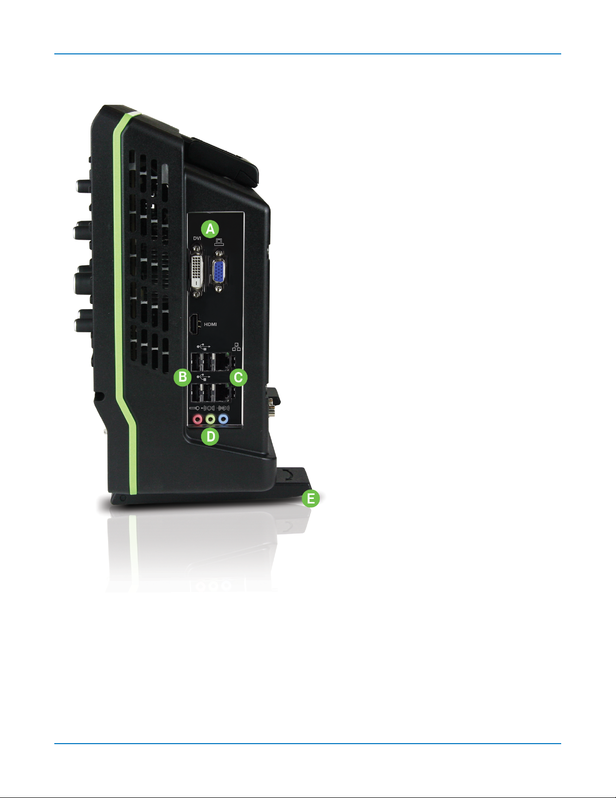
Side of Oscilloscope

A. DVI, VGA, and HDMI ports for external

monitor

B. USB 2.0 ports (4)

C. Ethernet ports (2) for connecting to LAN or

remote control

D. Audio In/Out (mic, speaker, and line-in) for

connecting external audio devices

E. Feet rotated back and flat

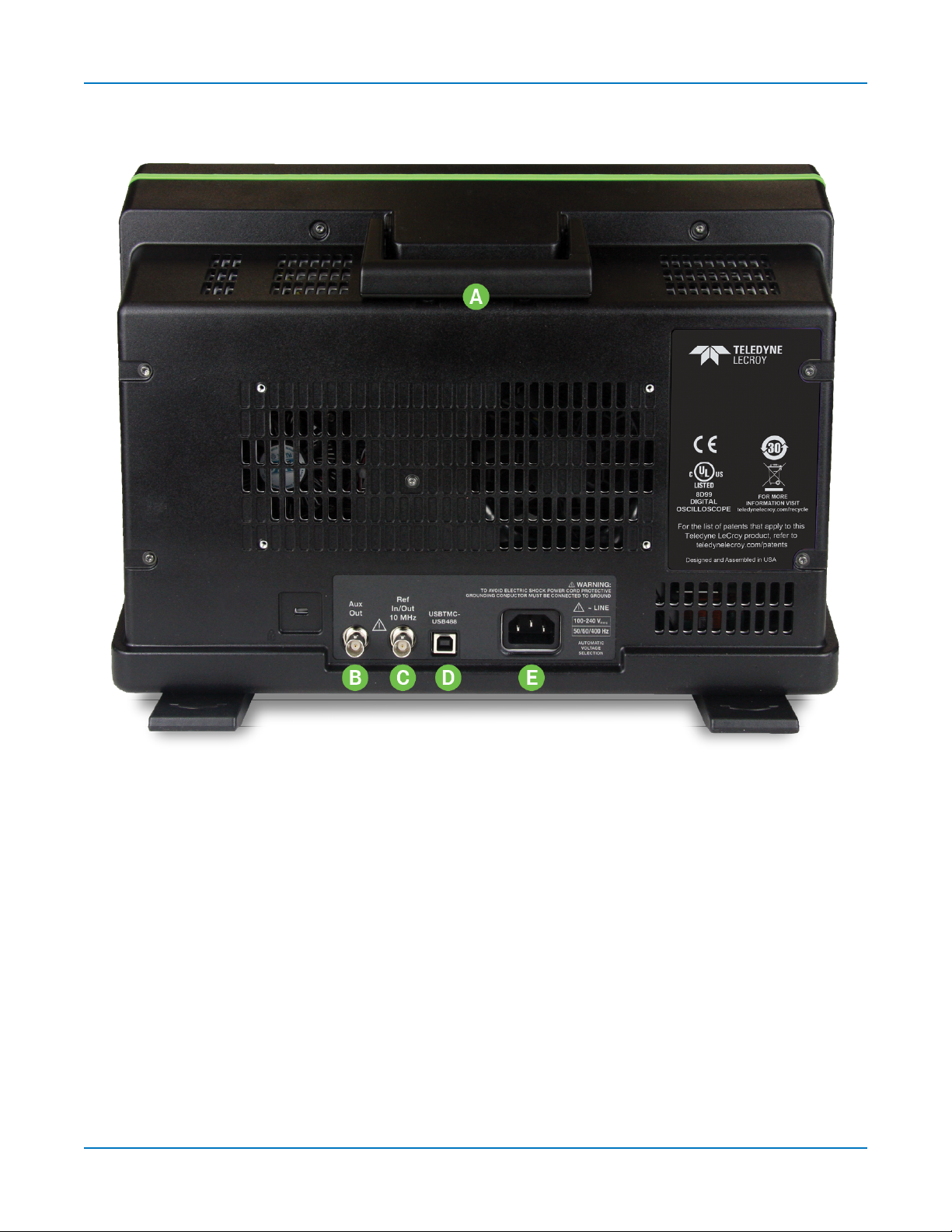
Back of Oscilloscope

Oscilloscope Overview

A. Built-in carrying handle

B. Aux Out

C. Ref In/Out for external reference clock

D. USBTMC port for remote control

E. AC power inlet

HDO6000/HDO6000A High Definition Oscilloscopes Operator's Manual

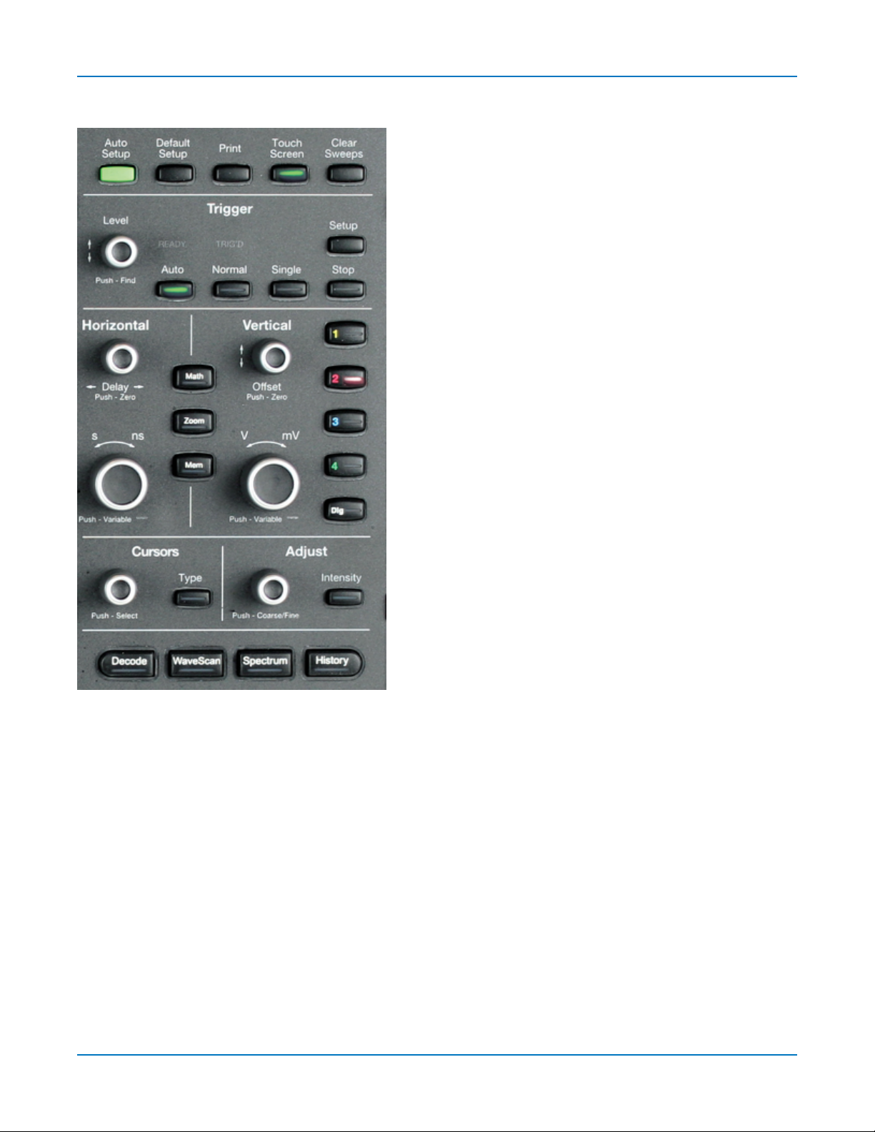
Front Panel

Front panel controlsduplicate functionality available through the touch screen and are described here only briefly.

Knobson the front panel function one way if turned and another if pushed like a button. The first label describes the knob’s “turn”action, the second label its “push” action. Actions performed from the front panel always apply to the active trace.

Many buttonslight to show the active traces and functions.

Trigger Controls

Level knob changes the trigger threshold level (V). The level isshown on the Trigger descriptor box. Pushing the knob sets the trigger level to the 50% point of the input signal.

READY indicator lights when the trigger isarmed. TRIG'D indicator is lit momentarily when a trigger occurs.

Setup opens/closes the Trigger Setup dialog.

Auto sweeps after a preset time, even if the trigger conditions are not met.

Normal sweeps each time the trigger signal meets the trigger conditions.

Single sets Single trigger mode. The first press readies the oscilloscope to trigger. The second pressarms and triggers the oscilloscope once (single-shot acquisition) when the input signal meets the trigger conditions.

Stop pauses acquisition. If you boot up the instrument with the trigger in Stop mode, a "No trace available" message is shown. Press the Auto button to display a trace.

Horizontal Controls

The Delay knob changes the Trigger Delay value (S) when turned. Push the knob to return Delay to zero.

The Horizontal Adjust knob sets the Time/division (S) of the acquisition system when the trace source is an input channel. The Time/div value is shown on the Timebase descriptor box. When using this control, the instrument allocates memory as needed to maintain the highest sample rate possible for the timebase setting. When the trace is a zoom, memory or math function, turn the knob to change the horizontal scale of the trace, effectively "zooming" in or out. By default, values adjust in 1, 2, 5 step increments. Push the knob to change to fine increments; push it again to return to stepped increments.

Oscilloscope Overview

Math, Zoom, and Mem(ory) Buttons

The Zoom button creates a quick zoom for each open channel trace. Touch the zoom trace descriptor box to display the zoom controls.

The Math and Mem(ory) buttons open the corresponding setup dialogs.

If a Zoom, Math or Memory trace isactive, the button illuminates to indicate that the Vertical and Horizontal knobs will now control that trace.

Vertical Controls

Offset knob adjusts the zero level of the trace (making it appear to move up/down relative to the center axis). The voltage value appears on the trace descriptor box. Push the knob to return Offset to zero.

Gain knob sets vertical scale (V/div). The voltage value appears on the trace descriptor box. By default, values adjust in 1, 2, 5 step increments. Push the knob to change to fine increments; push it again to return to stepped increments.

Channel (number) buttons turn on a channel that is off, or activate a channel that is already on. When the channel isactive, pushing its channel button turns it off. A lit button shows the active channel.

Dig button enables digital input through the Digital Leadset on instruments with the Mixed Signal option.

Cursor Controls

Cursors identify specific voltage and time values on a waveform. The white cursor markers help make these points more visible. A readout of the values appears on the trace descriptor box. There are five preset cursor types, each with a unique appearance on the display. These are described in more detail in the Cursors section.

Type selects the cursor type. Continue pressing to cycle through all cursor until the desired type is found. The type "Off" turns off the cursor display.

Cursor knob repositions the selected cursor when turned. Push it to select a different cursor to adjust.

Adjust and Intensity Controls

The front panel Adjust knob changes the value in active (highlighted) data entry fieldsthat do not have dedicated knobs. Pushing the Adjust knob toggles between coarse (large increment) or fine (small increment) adjustments.

When more data is available than can actually be displayed, the Intensity button helps to visualize significant events by applying an algorithm that dims lessfrequently occurring samples. This feature can also be accessed from the Display Setup dialog.

HDO6000/HDO6000A High Definition Oscilloscopes Operator's Manual

Miscellaneous Controls

Auto Setup performs an Auto Setup.

Default Setup restores the factory default configuration.

Print captures the entire screen and outputs it according to your Print settings. It can also be configured to output a LabNotebook entry.

Touch Screen enables/disables touch screen functionalilty.

Clear Sweeps resets the acquisition counter and any cumulative measurements.

Decode opens the Serial Decode dialog if you have serial data decoder options installed.

WaveScan opens the WaveScan dialog.

Spectrum opens the Spectrum Analyzer dialog if you have that option installed.

History opens the History Mode dialog.

Oscilloscope Overview

Signal Interfaces

The instrument offers a variety of interfaces for using probes or other devices to input analog or digital signals. See the product page at teledynelecroy.com for a list of compatible devices.

Analog Inputs

A series of connectors arranged on the front of the instrument are used to input analog signals on channels 1-4. EXT can be used to input an external trigger pulse or sample clock signal. AUX INon the back may also be used to input analog signal.

HDO channel connectors use the ProBus interface. The ProBus interface containsa 6-pin power and communication connection and a BNC signal connection to the probe. It includes sense rings for detecting passive probes and accepts a BNCcable connected directly to it. ProBus offers 50 Ω and 1 MΩ input impedance and control for a wide range of probes.

The channel interfaces power probes and completely integrate the probe with the channel. Upon connection, the probe type is recognized and some setup information, such as input coupling and attenuation, is performed automatically. This information is displayed on the Probe Dialog, behind the Channel (Cx) dialog. System (probe plus instrument) gain settings are automatically calculated and displayed based on the probe attenuation.

Probes

The oscilloscope is compatible with the included passive probes and most Teledyne LeCroy ProBus active probes that are rated for the instrument’s bandwidth. Probe specifications and documentation are available at teledynelecroy.com/probes.

Passive Probes

The passive probes supplied are matched to the input impedance of the instrument but may need further compensation. If using other passive probes, be sure to perform a low frequency calibration using the Cal signal available from the front panel before using them to measure signal. Follow the directionsin the probe instruction manual to compensate the frequency response of the probes.

Active Probes

Most active probes match probe to oscilloscope response automatically using probe response data stored in an on-board EEPROM. This ensures the best possible combined probe plus oscilloscope channel frequency response without the need to perform any de-embedding procedure.

Be aware that many active probes require a minimum oscilloscope firmware version to be fully operational. See the probe documentation.

HDO6000/HDO6000A High Definition Oscilloscopes Operator's Manual

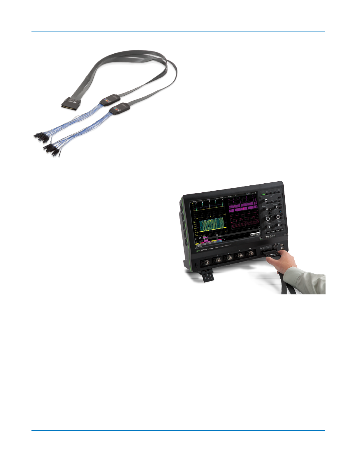
Digital Leadset

The digital leadset provided with -MS model oscilloscopes enables input of up-to-16 lines of digital data. Lines can be organized into four logical groups and renamed appropriately.

The digital leadset features two digital banks with separate Threshold controls, making it possible to simultaneously view data from different logic families.

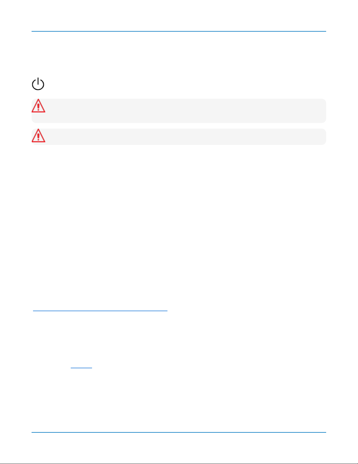
Connecting/Disconnecting the Leadset

The digital leadset connects to the Mixed Signal interface on the front of the instrument.

To connect the leadset to the instrument, push the connector into the Mixed Signal interface below the front panel until you hear a click.

To remove the leadset, press and hold the buttons on each side of the connector, then pull out to release.

Grounding Leads

Each flying lead has a signal and a ground connection. A variety of ground extenders and flying ground leads are available for different probing needs.

To achieve optimal signal integrity, connect the ground at the tip of the flying lead for each input used in your measurements. Use either the provided ground extenders or ground flying leads to make the ground connection.

Oscilloscope Set Up

Powering On/Off

Press the Power button to turn on the instrument. The X-Stream application loadsautomatically when you use the Power button.

Caution: Do not change the instrument’s Windows®Power Options setting from the default Never

to System Standby or System Hibernate. Doing so can cause the system to fail.

Caution: Do not power on or calibrate with a signal attached.

The safest way to power down the oscilloscope isto use the File > Shutdown menu option, which will always execute a proper shut down process and preserve settings. Quickly pressing the power button should also execute a proper shut down, but holding the Power button will execute a “hard” shut down (as on a computer), which we do not recommend doing because it does not allow the Windows operating system to close properly, and setup data may be lost. Never power off by pulling the power cord from the socket or powering off a connected power strip or battery without first shutting down properly.

The Power button does not disconnect the instrument from the AC power supply. The only way to fully power down the instrument is to unplug the AC power cord.

We recommend unplugging the instrument if it will remain unused for a long period of time.

Software Activation

The operating software (firmware and standard applications) isactive upon delivery. At power-up, the instrument loadsthe software automatically.

Firmware

Free firmware updates are available periodically from the Teledyne LeCroy website at:

teledynelecroy.com/support/softwaredownload

Registered users can receive an email notification when a new update is released. Follow the instructions on the website to download and install the software.

Purchased Options

If you decide to purchase an option, you will receive a license key via email that activates the optional features. See Options for instructionson activating optional software packages.

HDO6000/HDO6000A High Definition Oscilloscopes Operator's Manual

Connecting to Other Devices/Systems

Make all desired cable connections. After start up, configure the connections using the menu options listed below. More detailed instructions are provided later in this manual.

LAN

The instrument accepts DHCP network addressing. Connect a cable from an Ethernet port on the side panel to a network access device. Go to Utilities > Utilities Setup > Remote to find the IP address.

To assign a static IP address, choose Net Connections from the Remote dialog. Use the standard Windows networking dialogs to configure the device address.

Choose File > File Sharing and open the Email & Report Settings dialog to configure email settings.

USB Peripherals

Connect the device to a USB port on the front or side of the instrument. These connections are "plug-andplay" and do not require any additional configuration.

Printer

HDO oscilloscopes support USB printers compatible with the instrument's Windows OS. Go to File > Print Setup and select Printer to configure printer settings. Select Properties to open the Windows Print dialog.

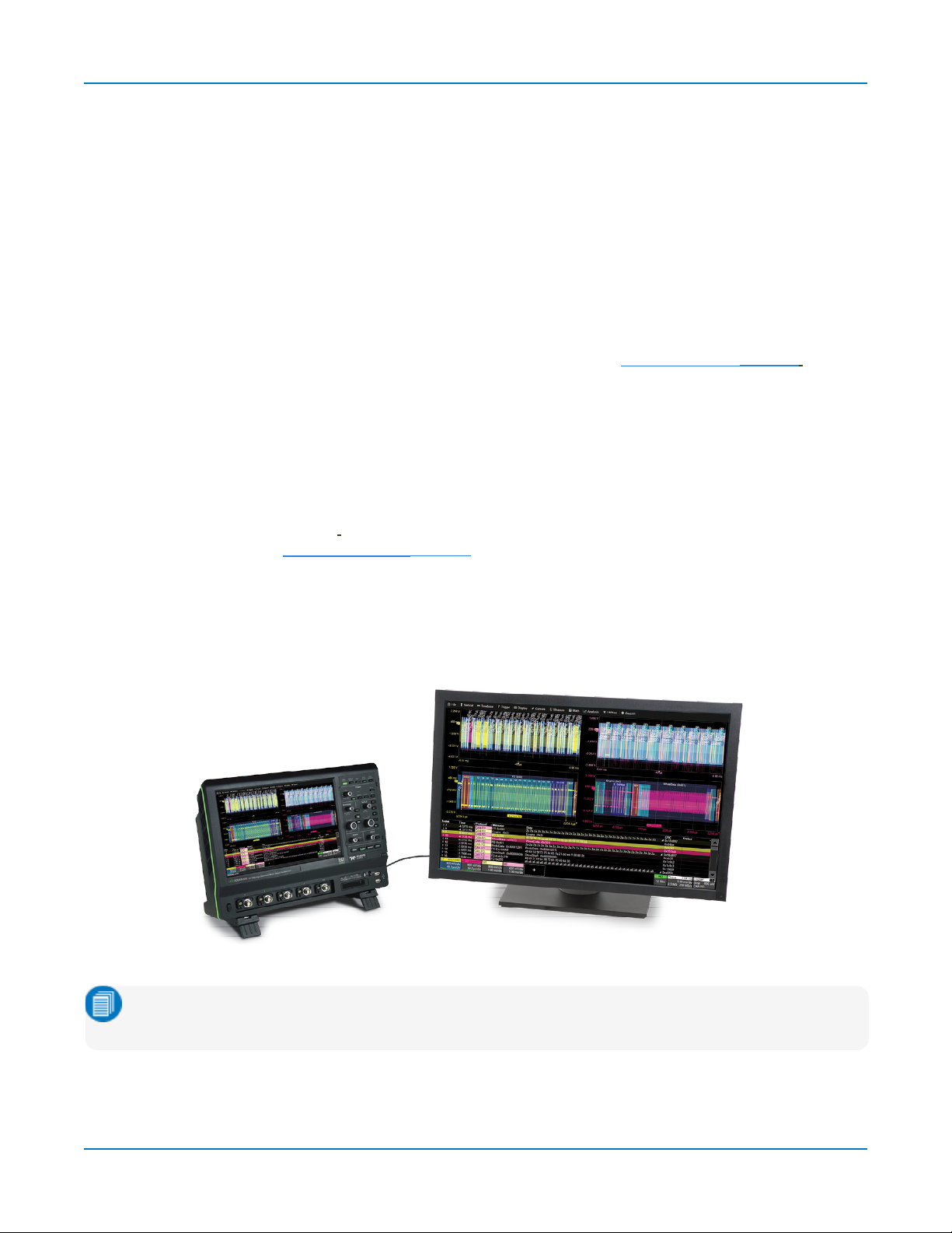
External Monitor

You may operate the instrument using the built-in touch screen or attach an external monitor for extended desktop operation.

Note: The oscilloscope display utilizes Fujitsu touch-screen drivers. Because of conflicts, external

monitorswith Fujitsu drivers can not be used to control the system, only as displays.

Oscilloscope Set Up

Connect the monitor cable to a video outputon the side of the instrument (VGA, DVI-D, and HDMI are all supported. Go to Display > Display Setup > Open Monitor Control Panel to configure the display. Be sure to select the instrument as the primary monitor.

To use the Extend Grids feature, configure the second monitor to extend, not duplicate, the oscilloscope display. If the external monitor is touch screen enabled, the MAUI user interface can be controlled through touch on the external monitor.

Remote Control

Go to Utilities > Preference Setup > Remote to configure remote control. Connect the devices using the cable type required by your selection. TCP/IP over Ethernet is generally supported.

Sample Clock

To input an external sample clock signal, connect a BNC cable from the EXT input to the other device. Go to Timebase > Horizontal Setup > Clock Source to configure the clock.

Reference Clock

To either input or output a reference clock signal, connect a BNC cable from the Ref In or Ref Out connector to the other instrument. Go to Timebase > Horizontal Setup > Clock Source to configure the

clock.

Auxilliary Output

To output signal from the instrument to another device, connect a BNCcable from Aux Out to the other device. Go to Utilities > Utilities Setup > Aux Output to configure the output.

HDO6000/HDO6000A High Definition Oscilloscopes Operator's Manual

Language Selection

To change the language that appears on the touch screen:

1. Go to Utilities > Preference Setup > Preferences and make a Language selection.

2. Follow the prompt to restart the application.

To also change the language of the Windowsoperating system dialogs:

1. Choose File > Minimize to hide X-Stream and show the Windows Desktop.

2. From the Windows task bar, choose Start > Control Panel > Clock, Language and Region.

3. Under Region and Language select Change Display Language.

4. Touch the Install/Uninstall Languages button.

5. Select Install Language and Browse Computer or Network.

6. Touch the Browse button, navigate to D:\Lang Packs\ and select the language you want to install. The available languages are: German, Spanish, French, Italian, and Japanese. Follow the installer prompts.

7. Reboot after changing the language.

Note: Other language packs are available from Microsoft’s website.

Using MAUI

MAUI, the Most Advanced User Interface, is Teledyne LeCroy'sunique oscilloscope user interface. MAUIis designed for touch—all important controls for vertical, horizontal, and trigger are only one touch away.

Touch Screen

The touch screen isthe principal viewing and control center. The entire display area is active: use your finger or a stylusto touch, drag, swipe, or draw a selection box.

Many controlsthat display information also work as “buttons” to access other functions. If you have a mouse installed, you can click anywhere you can touch to activate a control; in fact, you can alternate between clicking and touching, whichever is convenient for you.

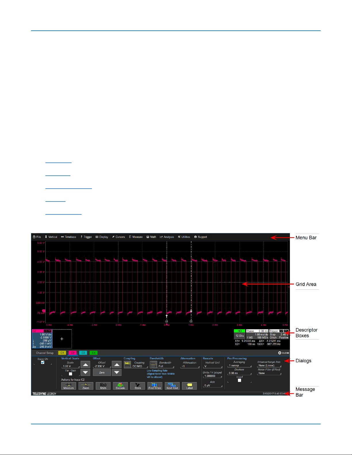
The touch screen isdivided into the following major control groups:

l Menu bar

l Grid area

l Descriptor boxes

l Dialogs

l Message Bar

HDO6000/HDO6000A High Definition Oscilloscopes Operator's Manual

Menu Bar

The top of the window contains a complete menu of functions. Making a selection here changes the dialogs displayed at the bottom of the screen.

While many common operations can also be performed from the front panel or launched via the descriptor boxes, the menu bar is the best way to access dialogs for Save/Recall (File) functions, Display functions, Status, LabNotebook, Pass/Fail setup, and Utilities/Preferences setup.

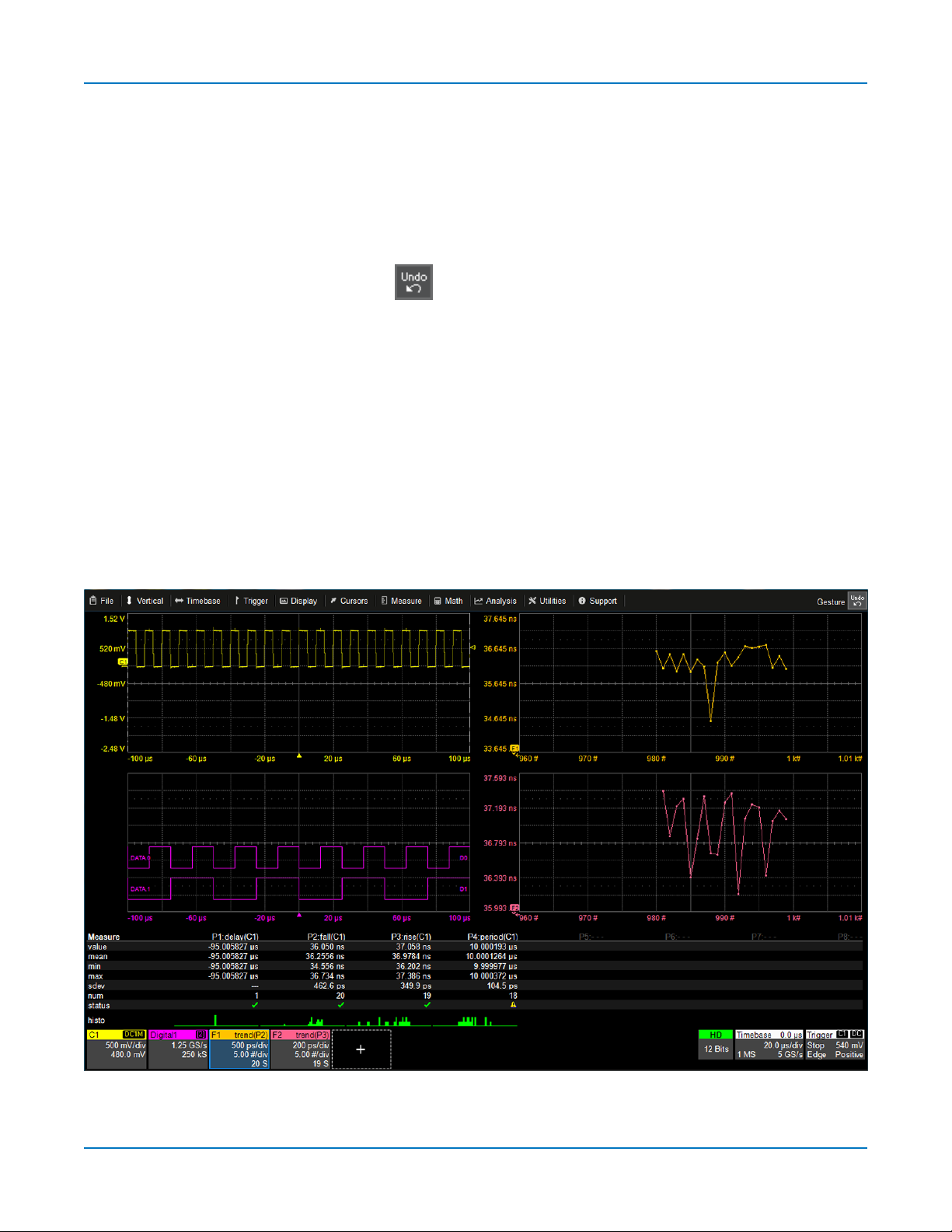
If an action can be “undone”, a small Undo button appears at the far right of the menu bar. Click this to restore the oscilloscope to the state prior to the action.

Grid Area

The grid area displays the waveform traces. Every grid is 8 Vertical divisions representing 4096 Vertical levels and 10 Horizontal divisions each representing acquisition time. The value represented by Vertical and Horizontal divisions depends on the Vertical and Horizontal scale of the traces that appear on the grid.

Multi-Grid Display

The grid area can be divided into multiple gridsshowing different types and numbers of traces (in Auto Grid mode, it will divide automatically as needed). Regardless of the number and orientation of grids, every grid always represents the same number of Vertical levels. Therefore, absolute Vertical measurement precision is maintained.

Different types of traces opening in a multi-grid display.

Using MAUI

Grid Indicators

These indicators appear around or on the grid to mark important points on the display. They are matched to the color of the trace to which they apply. When multiple traces appear on the same grid, indicators refer to the foreground trace—the one that appears on top of the others.

Axis labels

or change the Vertical/Horizontal scale. Originally shown in absolute values, the labels change to show delta from 0 (center) when the number of significant digits grows too large. The number of labels that appear on each grid depends on the total number of grids open. To remove them, go to Display > Display Setup and deselect Axis Labels.

Trigger Time

Unless Horizontal Delay is set, this indicator is at the zero (center) point of the grid. Delay time is shown at the top right of the Timebase descriptor box.

Pre/Post-trigger Delay

Delay has shifted the Trigger Position indicator to a point in time not displayed on the grid. All Delay values are shown on the Timebase Descriptor Box.

Trigger Level

in Stop trigger mode, or in Normal or Single mode without a valid trigger, a hollow triangle of the same color appears at the new trigger level. The trigger level indicator is not shown if the triggering channel is not displayed.

Zero Volts Level

the number and color of the trace.

Cursor markers

and-drop cursor markers to quickly reposition them.

Grid Intensity

mark the times/units represented by a grid division. They update dynamically as you pan the trace

, a small triangle along the bottom (horizontal) edge of the grid, shows the time of the trigger.

, a small arrow to the bottom left or right of the grid, indicates that a pre- or post-trigger

at the right edge of the grid tracks the trigger voltage level. If you change the trigger level when

is located at the left edge of the grid. One appears for each open trace on the grid, sharing

appear over the grid to indicate specific voltage and time values on the waveform. Drag-

You can adjust the brightness of the grid lines by going to Display > Display Setup and entering a new Grid Intensity percentage. The higher the number, the brighter and bolder the grid lines.

HDO6000/HDO6000A High Definition Oscilloscopes Operator's Manual

Descriptor Boxes

Trace descriptor boxes appear just beneath the grid whenever a trace is turned on. They function to:

l Inform—descriptors summarize the current trace settings and its activity status.

l Navigate—touch the descriptor box once to activate the trace, a second time to open the trace

setup dialog.

l Arrange—drag-and-drop descriptor boxes to move traces among grids.

l Configure—drag-and-drop descriptor boxes to change source or copy setups.

Besides trace descriptor boxes, there are also HD, Timebase and Trigger descriptor boxes summarizing the acquisition settings shared by all channels, which also open the corresponding setup dialogs.

Channel Descriptor Box

Channel trace descriptor boxes correspond to analog signal inputs. They show (clockwise from top left): Channel Number, Pre-processing list, Coupling, Vertical Scale (gain) setting, Vertical Offset setting, Sweeps Count (when averaging), Vertical Cursor positions, and Number of Segments (when in Sequence mode).

Codes are used to indicate pre-processing that hasbeen applied to the input. The short form isused when several processes are in effect.

Pre-processing Symbols on Descriptor Boxes

Pre-Processing Type Long Form Short Form

Sin X Interpolation* SINX S

Enhanced Sample Rate ESR E

Averaging AVG A

Inversion INV I

Deskew DSQ DQ

Coupling DC50, DC1M, AC1M or GND D50, D1, A1 or G

Bandwidth Limiting BWL B

Note: * On "A" models, (Sinx)/x interpolation is applied with the Enhanced Sample Rate feature.

The SINX symbol isreplaced by ESR.

Using MAUI

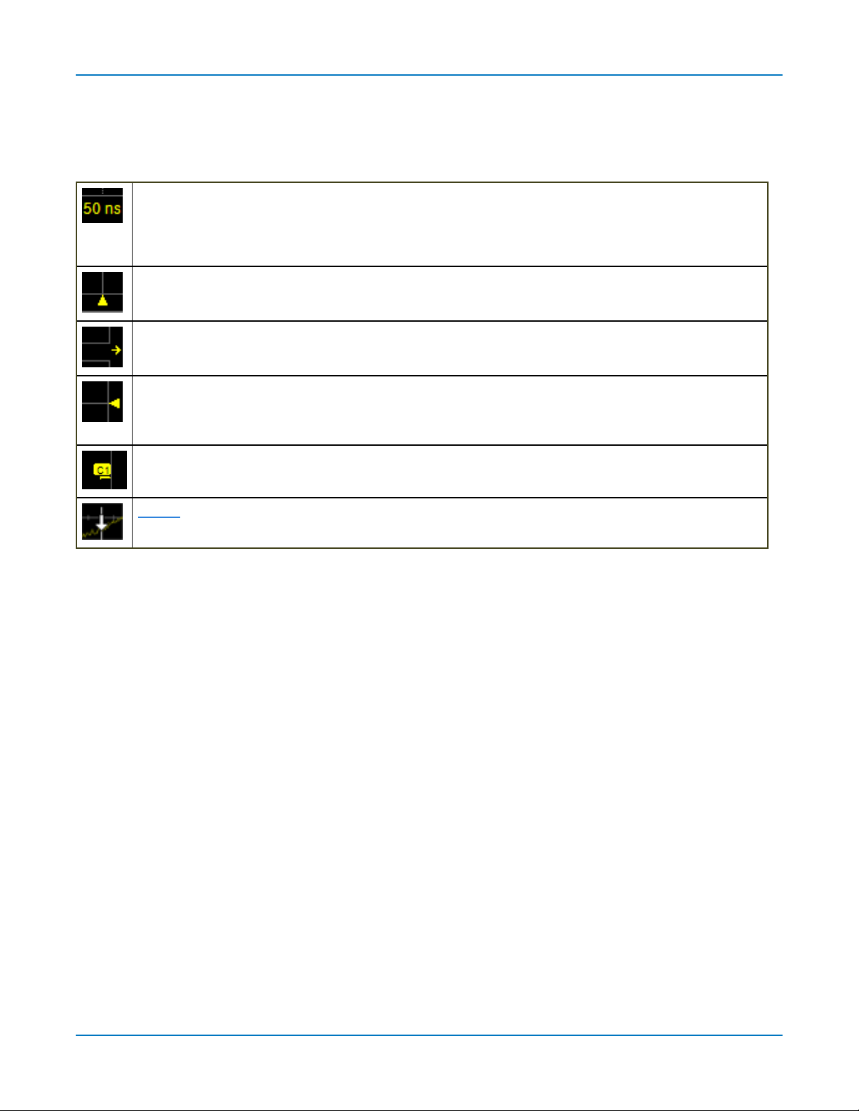
Other Trace Descriptor Boxes

Similar descriptor boxes appear for math (Fx), zoom (Zx), and memory (Mx) traces. These descriptor boxes show any Horizontal scaling that differs from the signal timebase. Units will be automatically adjusted for the type of trace.

Trace Context Menu

Touch and hold ("right-click") on the trace descriptor box until a white circle appears to open the trace context menu, a pop-up menu of actions to apply to the trace such as turn off, move to next grid or label.

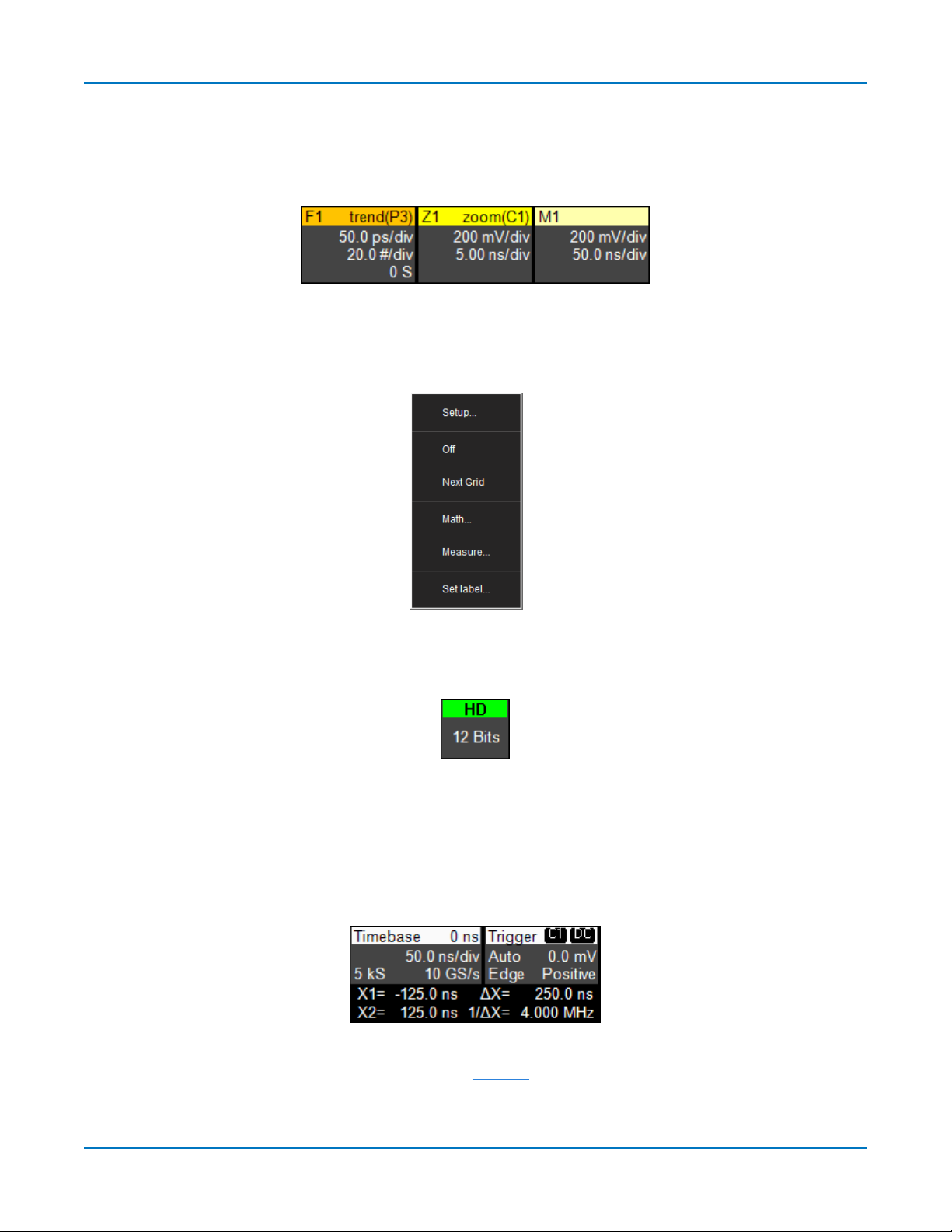
HD Descriptor Box

The HD descriptor box summarizes the ADC resolution at which the instrument is operating.

Timebase and Trigger Descriptor Boxes

The Timebase descriptor box shows: (clockwise from top right) Horizontal Delay, Time/div, Sample Rate, Number of Samples, and Sampling Mode (blank when in real-time mode).

Trigger descriptor box shows: (clockwise from top right) Trigger Source and Coupling, Trigger Level (V), Slope/Polarity, Trigger Type, Trigger Mode.

Horizontal (time) cursor readout, including the time between cursors and the frequency, isshown beneath the TimeBase and Trigger descriptor boxes. See the Cursors section for more information.

HDO6000/HDO6000A High Definition Oscilloscopes Operator's Manual

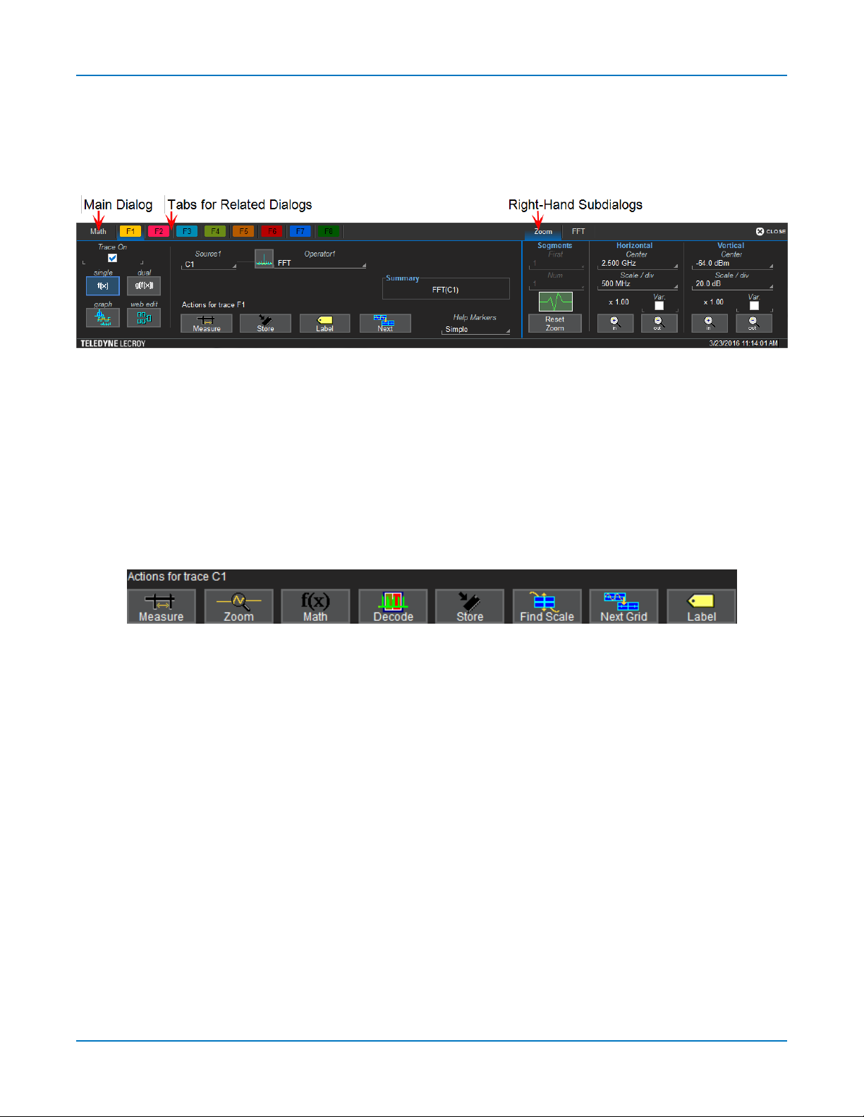
Dialogs

Dialogs appear at the bottom of the display for entering setup data. The top dialog will be the main entry point for the selected functionality. For convenience, related dialogs appear as a series of tabs behind the main dialog. Touch the tab to open the dialog.

Right-Hand Subdialogs

At times, your selections will require more settings than can fit on one dialog, or the task commonly invites further action, such as zooming a new trace. In that case, subdialogs will appear to the right of the dialog. These subdialog settingsalways apply to the object that is being configured on the left-hand dialog.

Action Toolbar

Several setup dialogscontain a toolbar at the bottom of the dialog. These buttons enable you to perform commonplace tasks—such as turning on a measurement—without having to leave the underlying dialog. Toolbar actionsalways apply to the active trace.

Measure opens the Measure pop-up to set measurement parameters on the active trace.

Zoom creates a zoom trace of the active trace.

Math opens the Math pop-up to apply math functions to the active trace and create a new math trace.

Decode opens the main Serial Decode dialog where you configure and apply serial data decoders and triggers. Thisbutton is only active if you have serial data software options installed.

Store loads the active trace into the corresponding memory location (C1, F1 and Z1 to M1; C2, F2 and Z2 to M2, etc.).

Find Scale performs a vertical scaling that fits the waveform into the grid.

Next Grid moves the active trace to the next grid. If you have only one grid displayed, a new grid will be created automatically, and the trace moved.

Label opens the Label pop-up to annotate the active trace.

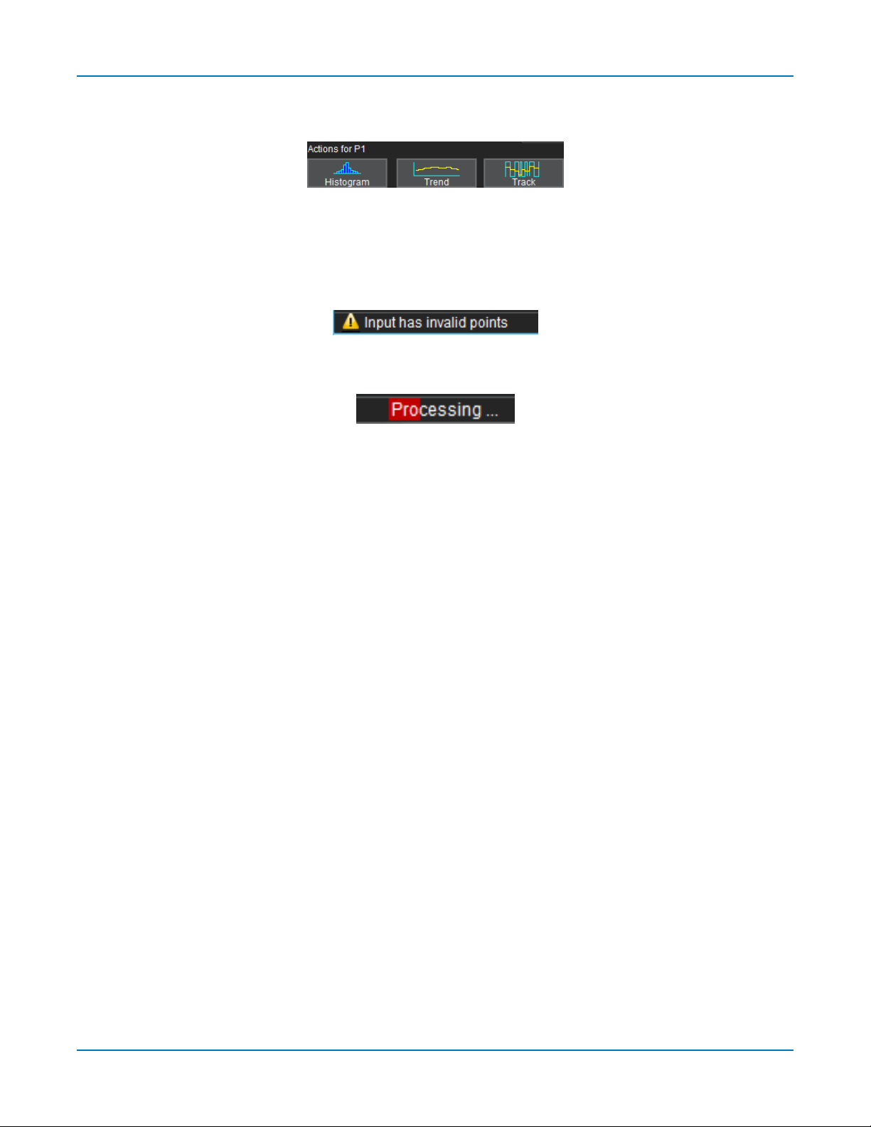
Using MAUI

Histogram, Trend, and Track buttons appear at the bottom of the Parameter (Px) dialogs. They allow you to create a Math function to plot the parameter while remaining on the measurement dialogs.

Message Bar

At the bottom of the oscilloscope display is a narrow message bar. The current date and time are displayed at the far right. Status, error, or other messages are also shown at the far left, where "Teledyne LeCroy" normally appears.

You will see the word "Processing..." highlighted with red at the right of the message bar when the oscilloscope is processing your last acquisition or calculating.

This willbe especially evident when you change an acquisition setting that affects the ADC configuration in Normal or Auto trigger mode, such as changing the Vertical Scale, Offset, or Bandwidth. Traces may briefly disappear from the display while the oscilloscope is processing.

HDO6000/HDO6000A High Definition Oscilloscopes Operator's Manual

OneTouch Help

Touch, drag, swipe, pinch, and flick can be used to create and change setups with one touch. Just as you change the display by using the setup dialogs, you can change the setups by moving different display objects. Use the setup dialogsto refine OneTouch actionsto precise values.

As you drag & drop objects, valid targets are outlined with a white box. When you're moving over invalid targets, you'll see the "Null" symbol ( Ø ) under your finger tip or cursor.

Note: Many actions shown here—such as Activate, Position Cursors, Change Trigger, Move Trace,

Scroll, Pan left/right, and Drag to Create Zoom—can be done on all MAUI instruments, even those without the OneTouch features. Some examples below may show features not available on your oscilloscope.

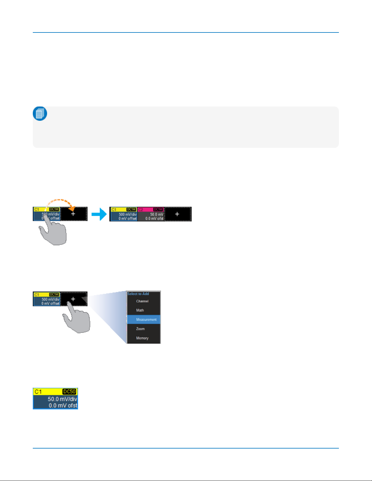
Turn On

To turn on a new channel, math, memory, or zoom trace, drag any descriptor box of the same type to the Add New ("+") box. The next trace in the series will be added to the display at the default settings. It is now the active trace.

If there is no descriptor box of the desired type on the screen to drag, touch the Add New box and choose the trace type from the pop-up menu.

To turn on the Measure table when it is closed, touch the Add New box and choose Measurement.

Activate

Touch a trace or its descriptor box to activate it and bring it to the foreground. When the descriptor box appears highlighted in blue, front panel controlsand touch screen gestures apply to that trace.

Using MAUI

Copy Setups

To copy the setup of one trace to another of the same type (e.g., channel to channel, math to math), drag-and-drop the source descriptor box onto the target descriptor box.

To copy the setup of a measurement (Px), drag-and-drop the source column onto the target column of the Measure table. You can do the same for a qualifier (Qx) on the Pass/Fail readout table.

Change Source

To change the source of a trace, drag-and-drop the descriptor box of the desired source onto the target descriptor box. You can also drop it on the Source field of the target setup dialog.

To change the source of a measurement, drag-and-drop the descriptor box of the desired source onto the parameter (Px) column of the Measure table. You can do the same to a qualifier (Qx) on the Pass/Fail readout table.

HDO6000/HDO6000A High Definition Oscilloscopes Operator's Manual

Position Cursors

To change cursor measurement time/level, drag cursor markers to new positions on the grid. The cursor readout will update immediately.

To place horizontal cursors on zoomsor other calculated traces where the source Horizontal Scale has forced cursors off the grid, drag the cursor readout from below the Timebase descriptor to the grid where you wish to place the cursors. The cursors are set at either the 5 (center) or 2.5 and 7.5 divisions of the grid. Cursors on the source traces adjust position accordingly.

Change Trigger

To change the trigger level, drag the Trigger Level indicator to a new position on the Y axis. The Trigger descriptor box will show the new voltage Level.

To change the trigger source channel, drag-and-drop the desired channel (Cx) descriptor box onto the Trigger descriptor box. The trigger will revert to the coupling and slope/polarity last set on that channel.

Using MAUI

Store to Memory

To store a trace to internal memory, drag-and-drop its trace descriptor box onto the target memory (Mx) descriptor box.

Move Trace

To move a trace to a different grid, drag-and-drop the trace descriptor box onto the target grid.

Scroll

To scroll long lists of values or readout tables, swipe the selection dialog or table in an up or down direction.

HDO6000/HDO6000A High Definition Oscilloscopes Operator's Manual

Pan Trace

To pan a trace, activate it to bring it to the forefront, then drag the waveform trace right/left or up/down. If it is the source of any other trace, that trace will move, as well. For channel traces, the Timebase descriptor box will show the new Horizontal Delay value. For other traces, the zoom factor controls show the new Horizontal Center.

Tip: If you are using the multi-zoom feature, all time-locked traces will pan together.

To pan at an accelerated rate, swipe the trace right/left or up/down.

Using MAUI

Zoom

To create a new zoom trace, touch then drag diagonally to draw a selection box around the portion of the trace you want to zoom. Touch the Zx descriptor box to open the zoom factor controlsand adjust the zoom exactly.

To "zoom in" on any trace, unpinch two fingers over the trace horizontally.

To "zoom out" on any trace, pinch two fingers over the trace horizontally.

Note: Pinch gestures do not create a separate zoom (Zx) trace, they only adjust the Horizontal

Scale. When you pinch a channel (Cx) trace, the Timebase for all channels changes. If the trace is the source of any other, all its dependent traces change, as well.

HDO6000/HDO6000A High Definition Oscilloscopes Operator's Manual

Turn Off

To turn off a trace, flick the trace descriptor box toward the bottom of the screen.

To turn off a measure parameter or Pass/Fail qualifier, flick the Px or Qx cell toward the bottom of the screen. If it's the last active cell of the table, the table will close.

Using MAUI

Working With Traces

Traces are the visible representations of waveforms that appear on the display grid. They may show live inputs(Cx, Digitalx), a math function applied to a waveform (Fx), a stored memory of a waveform (Mx), a zoom of a waveform (Zx), or the processing resultsof special analysissoftware.

Traces are a touch screen object like any other and can be manipulated. They can be panned, moved, labeled, zoomed, and captured in different visual formats for printing/reporting.

Each visible trace will have a descriptor box summarizing its principalconfiguration settings. See

OneTouch Help for more information about how you can use traces and trace descriptor boxes to modify

your configurations.

Active Trace

Although several traces may be open, only one trace is active and can be adjusted using front panel controls and touch screen gestures. A highlighted descriptor box indicates which trace is active. All actions apply to that trace untilyou activate another. Touch a trace descriptor box to make it the active trace (and the foreground trace in that grid).

Active trace descriptor (left), inactive trace descriptor (right).

Whenever you activate a trace, the dialog at the bottom of the screen automatically switches to the appropriate setup dialog.

Active descriptor box matches active dialog tab.

Foreground Trace

Since multiple traces can be opened on the same grid, the trace shown on top of the others is the foreground trace. Grid indicators (matched to the input channel color) represent values for the foreground trace.

Touch a trace or its descriptor box to bring it to the foreground. This also makes it the active trace.

Note that a foreground trace may not be the same as the active trace. A trace in a separate grid may subsequently become the active trace, but the indicators on a given grid will still represent the foreground trace in that group.

HDO6000/HDO6000A High Definition Oscilloscopes Operator's Manual

Turning On/Off Traces

Analog Traces

From the front panel, press the Channel button (1-4) to turn on the trace; press again to turn it off.

To turn on the trace from the touch screen, touch the Add New box and select Channel, or drag another Channel (Cx) descriptor box to the Add New box.

To turn off a channel trace from the touch screen, do any of the following:

l Flick the trace descriptor box toward the bottom of the screen.

l Touch-and-hold (right-click) on the descriptor box until a white circle appears, then from the context

menu select Off.

l Clear the "On" box on the Channel Setup or Cx dialogs.

Note: The default is to display each trace in its own grid. Use the Display menu to change how

traces are displayed.

Digital Traces

From the front panel, turn on the trace by pressing the Dig button, then checking Group on the Digitalx trace dialog.

To turn on the trace from the touch screen, choose Vertical > Digitalx Setup then check Group on the Digitalx dialog.

Clear the Group checkbox to turn off the trace, or flick the trace descriptor box toward the bottom of the screen.

Other Traces

From the touch screen, touch the Add New box and select the trace type, or drag another descriptor box of that type to the Add New box. Turn off the trace the same as you would a channel trace.

Adjusting Traces

To adjust Vertical Scale (gain or sensitivity) and Vertical Offset, just activate the trace and use the front panel Vertical knobs. To make other adjustments—such as channel pre-processing or the math function definition—touch the trace descriptor box twice to open the appropriate setup dialog.

Many entries can be made by selecting from the pop-up menu that appears when you touch a control. When an entry field appears highlighted in blue after touching, it is active and the value can be modified by turning the front panel knobs. Fields that don't have a dedicated knob (as do VerticalLevel and Horizontal Delay) can be modified using the Adjust knob.

If you have a keyboard installed, you can type entries in an active (highlighted) data entry field. Or, you can touch again, then "type" the entry by touching keys on the virtual keypad or keyboard.

Using MAUI

To use the virtual keypad, touch the soft keys exactly as you would a calculator. When you touch OK, the calculated value is entered in the field.

Moving Traces

Use any of these methods to move traces from grid to grid. See OneTouch Help for ways to pan traces within the same grid.

Drag-and-Drop

You can move a trace from one grid to another by dragging its descriptor box to the desired grid. This is a convenient way to quickly re-arrange traces on the display.

Next Grid Button

Touch twice on the descriptor box of the trace you want moved to open the setup dialog, then touch the Next Grid action toolbar button at the bottom of the dialog. You can also touch and hold (right-click) the trace descriptor box and choose Next Grid from the context menu.

Note: If only one grid is open, a second grid opens automatically when you select Next Grid.

HDO6000/HDO6000A High Definition Oscilloscopes Operator's Manual

Labeling Traces

The Label function gives you the ability to add custom annotationsto the trace display. Once placed, labels can be moved to new positions or hidden while remaining associated with the trace.

Create Label

1. Select Label from the context menu, or touch the Label Action toolbar button on the trace setup dialog.

2. On the Trace Annotation pop-up, touch Add Label.

3. Enter the Label Text.

4. Optionally, enter the Horizontal Pos. and Vertical Pos. (in same units as the trace) at which to place the label. The default position is 0 ns horizontal. Use Trace Vertical Position places the label immediately above the trace.

Reposition Label

Drag-and-drop labels to reposition them, or change the position settings on the Trace Annotation pop-up.

Edit/Remove Label

On the Trace Annotation pop-up, select the Label from the list. Change the settingsas desired, or touch Remove Label to delete it.

Clear View labels to hide all labels. They will remain in the list.

Using MAUI

Zooming

Zooms magnify a selected region of a trace by altering the Horizontal Scale relative to the source trace.

Zooms may be created in several ways, using either the front panel or the touch screen. You can adjust

zooms the same as any other trace using the front panel Vertical and Horizontal knobsor the touch screen

zoom factor controls.

The current settings for each zoom trace can be seen on the Zx dialogs, while the Zoom dialog is a convenient panel for turning on/off zoomsor changing the zoom source.

The MultiZoom feature creates time-locked zoom traces for only the waveforms that you choose to include. The zoomsare of the same X-axis section of each waveform. As you scrollthrough a waveform, all included zooms scroll in unison. For more information, refer to MultiZoom.

Zoom Dialog

Zoom controlsappear throughout the X-Stream software wherever it is likely you may wish to change the display scale of a trace, sometimes as a main dialog, sometimes asa subdialog, such as when setting up:

l Math traces on Fx dialogs

l Memory traces on Mx dialogs

To display the zoom controls, choose Math > Zoom Setup from the menu bar, or touch a zoom descriptor box.

The main Zoom dialog contains selection boxes for turning on/off and changing the source of a zoom. There are also optionsto:

l Reset All, return all zooms to x1 magnification.

l Quick Zoom, create a corresponding zoom trace for each open channel trace, same as using the

front panel Zoom button.

l MultiZoom

HDO6000/HDO6000A High Definition Oscilloscopes Operator's Manual

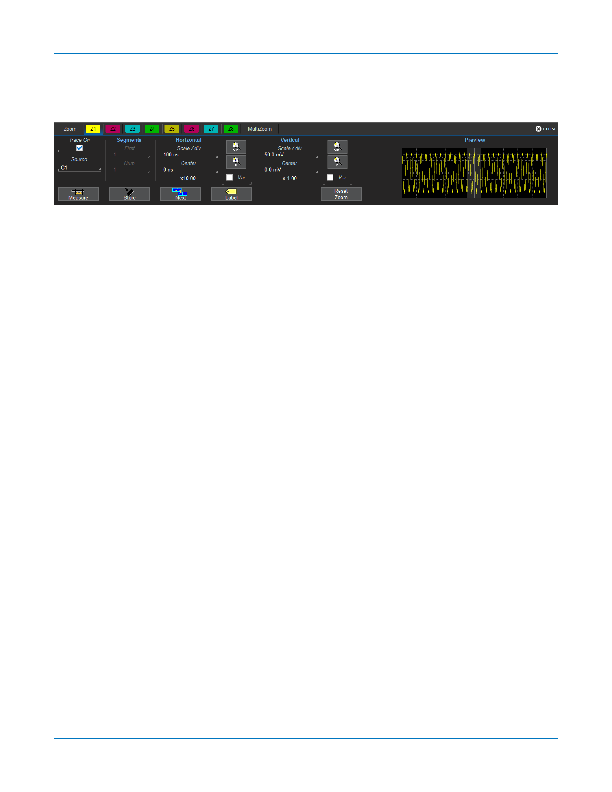
Zx Dialog

Behind the main Zoom dialog is a separate tab for each potential zoom trace (Z1-Zx). Each Zx dialog reflects the center and scale for that zoom. Use it to adjust the zoom magnification.

Trace Controls

Trace On shows/hides the zoom trace. It is selected by default when the zoom is created.

Source lets you change the source for this zoom to any channel, math, or memory trace while maintaining all other settings.

Segment Controls

These controls are used in Sequence Sampling Mode.

Zoom Factor Controls

l Out and In buttons increase/decrease zoom magnification and consequently change the Horizontal

andVertical Scale settings. Touch either button until you've achieved the desired level.

l Var.checkbox enables zooming in single increments.

l Horizontal Scale/div sets the time represented by each horizontal division of the grid. It is the

equivalent of Time/div in channel traces, only unlike that setting, it may differ for each zoom trace.

l Vertical Scale/div sets the voltage level represented by each vertical division of the grid; it's the

equivalent of V/div in channel traces.

l Horizontal/Vertical Center sets the time/voltage at the center of the grid. The horizontal center is

the same for all zoom traces.

l Reset Zoom returns the zoom to x1 magnification.

Using MAUI

Creating Zooms

Any type of trace can be "zoomed" by creating a new zoom trace (Zx) following the procedures here.

Note: On instruments with OneTouch, traces can be "zoomed" by pinching/unpinching two fingers

over the trace, but this method does not create a separate zoom trace. With channel traces, pinching will alter the acquisition timebase and the scale of all traces. Create a separate zoom trace if you do not wish to do this.

All zoom traces open in the next empty grid, with the zoomed portion of the source trace highlighted. If there are no more available grids, zoomswill open in the same grid as the source trace.

Zoomed area of original trace highlighted. Zoom in new grid below.

Quick Zoom

Use the front panel Zoom button to quickly create one zoom trace for each displayed channel trace. Quick zooms are created at the same vertical scale as the source trace and 10:1 horizontal magnification.

To turn off the quick zooms, press the Zoom button again.

Manually Create Zoom

To manually create a zoom, touch-and-drag diagonally to draw a selection box around any part of the source trace.

The zoom will resize the selected area to fit the fullwidth of the grid. The degree of vertical and horizontal magnification, therefore, depends on the size of the rectangle that you draw.

Alternatively, you can drag any Zx descriptor box over the Add New box, or touch the Add New box and choose Zoom from the pop-up menu. The next available zoom trace opens with its Zx dialog displayed for you to modify scale as needed.

Finally, you can touch-and-hold (right-click) on the descriptor box of the trace you

wish to zoom until a white circle appears, then choose Math from the context menu. Select the Zoom operator to create a zoom in the next open math function. Thismethod creates a new Fx trace, rather than a new Zx trace, but it can be rescaled in the same manner. It is a way to create more zoomsthan you have Zx slots available on your instrument.

HDO6000/HDO6000A High Definition Oscilloscopes Operator's Manual

Adjust Zoom Scale

The zoom's Horizontal units willdiffer from the signal timebase because the zoom is showing a calculated scale, not a measured level. Thisallows you to adjust the zoom factor using the front panel knobs or the

zoom factor controls however you like without affecting the timebase (a characteristic shared with math

and memory traces).

Close Zoom

New zooms are turned on and visible by default. If the display becomes too crowded, you can close a particular zoom and the zoom settings are saved in its Zx slot, ready to be turned on again when desired.

To close the zoom, touch-and-hold (right-click) on the zoom descriptor box until the white circle appears, then from the context menu choose Off.

MultiZoom

MultiZoom creates time-locked zoom traces for only the waveforms that you choose to include. The zooms are of the same X-axissection of each waveform. As you scroll through a waveform, allincluded zooms scrollin unison.

Set Up MultiZoom

1. Choose Math > Zoom Setup... to open the Zoom dialog, then touch the MultiZoom tab or MultiZoom Setup... button.

2. On the MultiZoom dialog, check On.

3. Select all the traces that are In the MultiZoom group.

Scroll Waveforms

The Auto-Scroll controls appear at the right of the MultiZoom dialog. They work similarly to A/V controls to allow you to continuously scroll all the selected zoom traces in time-locked steps from the beginning to the end of the acquisition.

Using MAUI

Print/Screen Capture

The front panel Print button captures an image of the display and outputs it according to your Print settings. It can be used to save a LabNotebook, create an image file of waveform traces, or send the display to a networked printer, etc.

The Printer icon at the right of the Print dialog will also execute your print setting.

Print may be used as a screen capture tool by going to File > Print Setup and selecting to print to File, then choosing a graphical format and naming scheme with your Screen Image Preferences. Once configured, just press the Print button or Printer icon, and optionally annotate the image.

You can also use the touch screen to generate a screen capture by choosing File > Save > Screen image and touching Save Now at the right of the dialog. The file issaved using your latest Screen Image Preferences settings.

HDO6000/HDO6000A High Definition Oscilloscopes Operator's Manual

Acquisition

The acquisition settings include everything required to produce a visible trace on screen and an acquisition record that may be saved for later processing and analysis:

l Vertical axis scale at which to show the input signal and probe characteristics that affect the signal,

such as attenuation and deskew time

l Horizontal axis scale at which to represent time, and acquisition sampling mode and sampling rate

l Acquisition trigger mechanism

Optional acquisition settings include bandwidth filters and pre-processing effects, vertical offset, and horizontal trigger delay, all of which affect the appearance and position of the waveform trace.

To avoid aliasing and other waveform distortions, it is advisable (per Nyquist) to acquire at a sample rate at least twice the bandwidth of the input signal. It can be shown that a sample rate 10 times the acquisition bandwidth is preferable in order to over sample fast signal rise times consistent with the oscilloscope bandwidth.

Those with higher speed acquisition systems may need to manually adjust Bandwidth, Time/div, Sample Rate, and the number of Active Channels to achieve the optimal result. Most Teledyne LeCroy oscilloscopes have a Fixed Sample Rate option, which uses whatever memory is required for the acquisition time, until none remains.

Auto Setup

Auto Setup quickly configures the essential acquisition settings based on the first input signal it finds, starting with Channel 1. If nothing is connected to Channel 1, it searches Channel 2 and so forth untilit finds a signal. Vertical Scale (V/div), Offset, Timebase (Time/div), and Trigger are set to an Edge trigger on the first, non-zero-level amplitude, with the entire waveform visible for at least 10 cycles over 10 horizontal divisions.

To run Auto Setup:

1. Either press the front panel Auto Setup button or choose Auto Setup from the Vertical, Timebase, or Trigger menus. All these options perform the same function.

2. Press the Auto Setup button again or use the touch screen display to confirm Auto Setup.

After running Auto Setup, you'll see the words"Auto Setup" next to an Undo button at the far right of the menu bar. Thisallowsyou to restore the settings in place prior to the Auto Setup.

Note: You will undo all new measurements or math function definitions entered since the Auto

Setup when you Undo the Auto Setup. Perform this work when the instrument is not in the Auto Setup mode if you wish for it to persist.

HDO6000/HDO6000A High Definition Oscilloscopes Operator's Manual

Viewing Status

All instrument settingscan be viewed through the various Status dialogs. These show all existing acquisition, trigger, channel, math function, measurement and parameter configurations, as well as which are currently active.

Access the Status dialogsby choosing the Status option from the Vertical, Timebase, Math, or Analysis menus (e.g., Channel Status, Acquisition Status).

Vertical

Vertical, also called Channel, settings usually relate to voltage level and control input channel traces (C1Cx) along the Y axis.

Note: While Digital settings can be accessed through the Vertical menu on -MS model

instruments, they are handled quite differently. See Digital.

The amount of voltage displayed by one vertical division of the grid, or Vertical Scale (V/div), ismost quickly adjusted by using the front panel Vertical knob. The Cx descriptor box always showsthe current Vertical Scale setting.

Detailed configuration for each trace is done on the Cx dialogs. Once configured, channel traces can be quickly turned on/off or modified using the Channel Setup dialog.

Channel Setup Dialog

Use the Channel Setup dialog to quickly make basic Vertical settings for all analog input channels. To access the Channel Setup dialog, choose Vertical > Channel Setup from the menu bar.

To show/hide the channel trace, select/deselect the checkbox next the channel number.

To change the channel trace color, touch the color block next to the channel number, then choose the new color from the pop-up menu.

Acquisition

To change any other Vertical settings, touch the input field and enter the new value.

On instruments with OneTouch, drag-and-drop the source channel descriptor box onto the target channel descriptor box to copy settings from one channel to another

You can also touch Copy Channel Setup, then select the channel to Copy From and all the channels to Copy To.

Cx (Channel) Dialog

Full vertical setup is done on the Cx dialog. To access it, choose Vertical > Channel <#> Setup from the menu bar, or touch the Channel descriptor box.

The Cx dialog contains:

l Vertical settings for scale, offset, coupling, bandwidth, and probe attenuation

l Rescale settings

l Pre-processing settings for pre-acquisition processes such asnoise filtering and interpolation.

If a Teledyne LeCroy probe isconnected, its Probe dialog appears to the right of the Cx dialog.

Vertical Settings

The Trace On checkbox turns on/off the channel trace.

Vertical Scale sets the gain (sensitivity) in the selected Vertical units, Volts by default. Select Variable Gain for fine adjustment or leave the checkbox clear for fixed 1, 2, 5, 10-step adjustments.

Offset adds a defined value of DC offset to the signal as acquired by the input channel. This may be helpful in order to display a signal on the grid while maximizing the vertical height (or gain) of the signal. A negative value of offset will "subtract" a DC voltage value from the acquired signal (and move the trace down on the grid") whereas a positive value willdo the opposite. Touch Zero Offset to return to zero.

A variety of Bandwidth filters are available. To limit bandwidth, select a filter from this field.

Coupling may be set to DC 50 Ω, DC1M, AC1M or GROUND.

Caution: The maximum input voltage depends on the input used. Limits are displayed on the body

of the instrument. Whenever the voltage exceeds this limit, the coupling mode automatically switches to GROUND. You then have to manually reset the coupling to its previous state. While the unit does provide this protection, damage can still occur if extreme voltages are applied.

HDO6000/HDO6000A High Definition Oscilloscopes Operator's Manual

Probe Attenuation and Deskew

Probe Attenuation and Deskew values for third-party probes may be entered manually on the Cx dialog. The instrument will detect it is a third-party probe and display these fields.

When a Teledyne LeCroy probe isconnected to a channel input:

l Passive probe Attenuation is automatically set, and this field is disabled on the Cx dialog.

l For active voltage and current probes, a tab isadded to the right of the Cx tab. The Attenuation field

becomes a button to access the Probe dialog. Enter Attenuation on the Probe dialog.

l Enter Deskew under Pre-Processing settings.

Rescale Settings

The rescale function allows you to apply a multiplication factor, additive constant, and differential vertical unit to the waveform vertical samples.

Vertical Units may be changed from Volts(V) to Amperes (A). This is useful when using a third-party current probe (which is not auto-detected) or when probing across a current sensor/resistor.

Enter the desired values in Units/V and Add. These two selections provide the same capability as the Rescale math function (y=mx+b) but in a more intuitive, user-friendly format.

Pre-Processing Settings

Average performs continuous averaging or the repeated addition, with unequal weight, of successive source waveforms. It is particularly useful for reducing noise on signals drifting very slowly in time or amplitude. The most recently acquired waveform has more weight than all the previously acquired ones: the continuousaverage is dominated by the statistical fluctuationsof the most recently acquired waveform. The weight of old waveforms in the continuous average gradually tends to zero (following an exponential rule) at a rate that decreases asthe weight increases.

On legacy HDO6000 models, Interpolate applies either Linear or (Sinx)/x interpolation to the waveform. Linear inserts a straight line between sample points and is best used to reconstruct straight-edged signals such as square waves. (Sinx)/x interpolation, on the other hand, is suitable for reconstructing curved or irregular wave shapes, especially when the sample rate is3 to 5 times the system bandwidth.

On "A" models, this setting is called Enhanced Sample Rate and appears disabled when using a sample rate greater than 2.5 GS/s, as the system automatically sets the upsample factor according to your sample rate. Only when the sample rate isbelow this can you choose an upsample factor of 2 or 4 points, or use Linear interpolation (None).

Note: 10 point Sinx/x interpolation can be set by sending the command via IEEE488.2 remote

control or COM Automation.

Deskew adjusts the horizontal time offset by the amount entered in order to compensate for propagation delays caused by different probes or cable lengths. The valid range is dependent on the current timebase setting. The Deskew pre-processing setting and the Deskew math function perform the same action.

Acquisition

Noise Filter applies Enhanced Resolution (ERes) filtering to increase vertical resolution, allowing you to distinguish closely spaced voltage levels. The tradeoff isreduced bandwidth. The functioning of the instrument's ERes is similar to smoothing the signal with a simple, moving-average filter. It is best used on single-shot acquisitions, acqusitions where the data record isslowly repetitive (and you cannot use averaging), or to reduce noise when your signal is noticeably noisy but you do not need to perform noise measurements. It also may be used when performing high-precision voltage measurements and zooming with high vertical gain, for example. See Enhanced Resolution.

Invert inverts the trace.

Probe Dialog

The Probe Dialog immediately to the right of the Cx dialog displaysthe probe attributes and (depending on the probe type) allows you to AutoZero or DeGauss probes from the touch screen. Other settings may appear, as well, depending on the probe model.

Caution: Remove probes from the circuit under test before initializing AutoZero or DeGauss.

Auto Zero Probe

Auto Zero corrects for DC offset drifts that naturally occur from thermal effects in the amplifier of active probes. Teledyne LeCroy probes incorporate Auto Zero capability to remove the DC offset from the probe's amplifier output to improve the measurement accuracy.

DeGauss Probe

The Degauss controlisactivated for some types of probes (e.g., current probes). Degaussing eliminates residual magnetization from the probe core caused by external magnetic fieldsor by excessive input. It is recommended to always Degauss probes prior to taking a measurement.

HDO6000/HDO6000A High Definition Oscilloscopes Operator's Manual

Digital (Mixed Signal)

The digital leadset (standard with -MS model oscilloscopes) inputs up-to-16 lines of digital data. Leads are organized into two banks of eight leads each, and you assign each bank a standard Logic Family or a custom Threshold to define the digital logic of the signal.

Digital Traces

When a digital group is enabled, digital Line traces show which lines are high, low, or transitioning relative to the threshold. You can also view a digital Bus trace that collapses all the lines in a group into their Hex values.

Four digital lines displayed with a Vertical Position +4.0 (top of grid) and a Group Height 4.0 (divisions).

Activity Indicators

Activity indicators at the bottom of the Digitalx dialogsshow which lines are High (up arrow), Low (down arrow), or Transitioning (up an down arrows) relative to the Logic Threshold value. They provide a quick view of which lines are active and of interest to display on screen.

Acquisition

Digitalx (Group) Set Up

To set up a digital input:

1. Connect the digital leadset to the test device and the instrument.

2. From the menu bar, choose Vertical > Digital <#> Setup, or pressthe front panel Dig button and select the desired Digitalx tab.

3. On the Digitalx set up dialog, check the boxes for all the lines that comprise the group. Touch the Right and Left Arrow buttons to switch between digital banks as you make line selections.

Alternatively, touch Display Dxx-Dyy to quickly turn on an entire digital bank.

Note: Each group can consist of anywhere from 1 to 16 of the leads from any digital bank

regardless of the Logic set on the bank. It does not matter if the some or allof the lines have been included in other groups.

4. Check View Group to enable the display.

5. When you're finished on the Digitalx dialog, open Logic Setup and choose the Logic Family that applies to each digital bank, or set custom Threshhold and Hysteresis values.

6. Go on to set up the digital display for the group.

HDO6000/HDO6000A High Definition Oscilloscopes Operator's Manual

Digital Display Set Up

Choose the type and position of the digital traces that appear on screen for each digital group.

1. Set up the digital group.

2. Choose a Display Mode:

l Lines (default) shows a time-correlated trace indicating high, low, and transitioning points

(relative to the Threshold) for every digital line in the group. The size and placement of the lines depend on the number of lines, the Vertical Position and GroupHeight settings.

l Bus collapses the lines in a group into their Hex values. It appears immediately below all the

Line traces when both are selected.

l Lines & Bus displays both line and bus traces at once.

3. In Vertical Position, enter the number of divisions (positive or negative) relative to the zero line of the grid where the display begins.The top of the first trace appears at this position.

4. In Group Height, enter the total number of grid divisions the entire display should occupy. All the selected traces (Line and Bus) will appear in thismuch space. Individualtraces are resized to fit the total number of divisions available.

The example above shows a group of four Line traces occupying a Group Height of 4.0 divisions. Each trace takes up one division.

To close digital traces, uncheck the Group box on the Digitalx dialog.

Tip: Because a new grid opens to accommodate each enabled group, you may wish to enable

groupsone or two at a time when they have many lines to maximize the total amount of screen space available for each. Closing the set up dialogswill also increase available screen space.

Acquisition

Renaming Digital Lines

The labels used to name each line can be changed to make the user interface more intuitive. Also, labels can be "swapped" between lines.

Changing Labels

1. Set up the digital group.

2. Touch Label and select from:

l Data - the default, which appends "D." to the front of each line number.

l Address - appends "A." to the front of each line number.

l Custom - lets you create your own labels line by line.

3. If using Custom labels:

l Touch the Line number field below the corresponding checkbox. If necessary, use the

Left/Right Arrow buttons to switch between banks.

l Use the virtual keyboard to enter the name, then press OK.

Any active line traces are renamed accordingly.

Swapping Lines

This procedure helps in cases where the physical lead number is different from the logical line number you would like to assign to that input. It can save time having to re-attach leads or re-configure groups.

Example: A group is set up for lines 0-4, but lead 5 was accidentally attached to the probing point. By "swapping" line 5 with line 4, you do not need to change either the physical or the logical setup.

1. Select a Label of Data or Address.

2. Touch the Line number button below the corresponding checkbox. If necessary, use the Left/Right Arrow buttons to switch between banks.

3. From the pop-up, choose the line with which you want to swap labels.

The button and any active line traces are renumbered accordingly.

HDO6000/HDO6000A High Definition Oscilloscopes Operator's Manual

Timebase

Timebase, also known as Horizontal, settings control the trace along the X axis. The timebase is shared by all channels.

The time represented by each horizontal division of the grid, or Time/Division, ismost easily adjusted using the front panel Horizontal knob. FullTimebase set up, including sampling mode and clock source selection, isdone on the Timebase dialog, which can be accessed by either choosing Timebase > Horizontal Setup from the menu bar or touching the Timebase descriptor box.

Timebase Set Up

Use the Timebase dialog to select the sampling mode, memory /sample rate,. You can also use it instead of the Front Panel to modify the Time/Div and horizontal Delay. There are related dialogs for Clock Source.

Sampling Mode

Choose from Real Time, Sequence, RIS, or Roll mode.

Timebase Mode

Time/Division isthe time represented by one horizontal division of the grid. Touch the Up/Down Arrow buttons on the Timebase dialog or turn the front panel Horizontal knob to adjust this value. The overall length of the acquisition record is equal to 10 times the Time/Division setting.

Delay is the amount of time relative to the trigger event to display on the grid. Raising/lowering the Delay value hasthe effect of shifting the trace to the right/left. This allowsyou to isolate and display a time/event of interest that occurs before or after the trigger event.

l Pre-trigger Delay, entered as a negative value, displaysthe acquisition time prior to the trigger event,

which occurs at time 0 when in Real Time sampling mode. Pre-trigger Delay can be set up to the instrument's maximum sample record length; how much actual time this represents depends on the timebase. At maximum pre-trigger Delay, the trigger position is off the grid (indicated by the arrow at the lower right corner), and everything you see represents 10 divisions of pre-trigger time.

l Post-trigger Delay, entered as a positive value, displays time following the trigger event. Post-trigger

Delay can cover a much greater lapse of acquisition time than pre-trigger Delay, up to the equivalent of 10,000 divisions after the trigger event occurred (it is limited at slower time/div settings and in Roll mode sampling). At maximum post-trigger Delay, the trigger point is off the grid far left of the time displayed.

Set to Zero returns Delay to zero.

Acquisition

Real Time Sampling Rate

These controls specify how the instrument samples when in Real Time mode.

Maximum Sample Points is the number of samples taken per acquisition when you choose to Set Maximum Memory. It changes to show Sampling Rate, the number of samples taken per time division, when using a Fixed Sampling Rate.

Set Maximum Memory, the default setting on MAUI oscilloscopes, automatically adjusts the sampling rate to take the maximum number of samples possible given the amount of pre- or post-trigger Delay and the Time/div, up to the maximum record length. This optimizes the sample rate for fast timebases when in Real Time mode.

Fixed Sampling Rate activates the Sampling Rate field for you to set your own rate. Lowering the rate can extend the acquisition to accommodate slower timebases or longer delays. On "A" models, if you choose a rate greater than 2.5 GS/s, the system will automatically enter Enhanced Sample Rate, applying Sinx/x Interpolation to prevent aliasing at the higher sample rate. An upsample factor of 2 pts. isused for 5 GS/s timebases, or 4 pts. for 10 GS/s and higher timebases. At lower rates, you can set the Enhanced Sample Rate factor yourself on the Cx dialog, or choose to use Linear interpolation.

Sampling Modes

The Sampling Mode determines how the instrument samples the input signal and renders it for display.

Real Time Sampling Mode

Real Time sampling mode is a series of digitized voltage values sampled on the input signal at a uniform rate. These samples are displayed as a series of measured data values associated with a single trigger event. By default (with no Delay), the waveform is positioned so that the trigger event is time 0 on the grid. The relationship between sample rate, memory, and time can be expressed as:

Capture Interval = 1/Sample Rate X Memory Capture Interval/10 = Time Per Division

Usually, on fast timebase settings, the maximum sample rate is used when in Real Time mode. For slower timebase settings, the sample rate is decreased so that the maximum number of data samples is maintained over time.

Roll Sampling Mode

Roll mode displays, in real time, incoming points in single-shot acquisitions that appear to "roll" continuously across the screen from right to left untila trigger event is detected and the acquisition is complete. The parameters or math functions set on each channel are updated every time the rollmode buffer is updated as new data becomes available. This resets statistics on every step of Roll mode that is valid because of new data.

Timebase must be set to 100 ms/div or slower to enable Roll mode selection. Rollmode samples at ≤ 2.5 MS/s. Only Edge trigger issupported.

Note: If the processing time is greater than the acquire time, the data in memory is overwritten. In

this case, the instrument issues the warning, "Channel data isnot continuous in ROLL mode!!!" and rolling starts again.

HDO6000/HDO6000A High Definition Oscilloscopes Operator's Manual

RIS Sampling Mode

RIS (Random Interleaved Sampling) allowseffective sampling rates higher than the maximum single-shot sampling rate. It is available on timebases ≤ 10 ns/div.

The maximum effective RIS sampling rate is achieved by making multiple single-shot acquisitions at maximum real-time sample rate. The bins thus acquired are positioned approximately 8 ps (125 GS/s) apart. The process of acquiring these bins and satisfying the time constraint isa random one. The relative time between ADC sampling instants and the event trigger provides the necessary variation.

Because the instrument requires multiple triggers to complete an acquisition, RIS is best used on repetitive waveforms with a stable trigger. The number depends on the sample rate: the higher the sample rate, the more triggers are required. It then interleaves these segments (as shown in the following illustration) to provide a waveform covering a time interval that is a multiple of the maximum single-shot sampling rate. However, the real-time interval over which the instrument collects the waveform data is much longer, and depends on the trigger rate and the amount of interleaving required.

Sequence Sampling Mode

In Sequence Mode sampling, the completed waveform consists of a number of fixed-size segments. The instrument uses the Timebase Sequence settings to determine the capture duration of each segment. The desired number of segments, maximum segment length, and total available memory are used to determine the actual number of samples or segments, and time or points.

Sequence Mode is ideal when capturing many fast pulses in quick succession or when capturing few events separated by long time periods. The instrument can capture complicated sequences of events over large time intervals in fine detail, while ignoring the uninteresting periods between the events. Measurements can be made on selected segments using the full precision of the timebase.

Sequence Mode Set Up The Sequence dialog appears only when Sequence Mode sampling is selected. Use it to define the

number of fixed-size segments to be acquired in single-shot mode.

1. From the menu bar, choose Timebase > Horizontal Setup..., then Sequence Sampling Mode.

2. On the Sequence tab under Acquisition Settings, enter the Number of Segments to acquire.

Note: The number of segments displayed can be less than the total number acquired.

3. To stop acquisition in case no valid trigger event occurs within a certain timeframe, check the Enable Timeout box and provide a Timeout value.

Note: While optional, Timeout ensures that the acquisition completes in a reasonable

amount of time and control is returned to the operator/controller without having to manually stop the acquisition, making it especially useful for remote control applications.

4. Touch Display mode and select a sequence display mode from the pop-up menu:

Acquisition

Adjacent

Waterfall (cascaded)

Mosaic (tiled)

Overlay

Perspective

5. Touch one of the front panel Trigger buttons to begin acquisition.

Tip: You can interrupt acquisition at any time by pressing the front panel Stop button. In this

case, the segments already acquired will be retained in memory.

View Sequence Segments When in Sequence sampling mode, you can view individual segments easily using the front panel Zoom

button. A new zoom of the channel trace defaults to Segment 1.

You can view other segments by changing the First and total Num(ber) of segments to be shown on the Zx dialog. Touch the Zx descriptor box to display the dialog.

Tip: By setting the Num value to 1, you can use the front panel Adjust knob to scroll through each

segment in order.

Channel descriptor boxes indicate the total number of segments acquired in sequence mode. Zoom descriptor boxes show the first segment displayed and total number of segments displayed ([#] #). As with all other zoom traces, the zoomed segments are highlighted on the source trace.

HDO6000/HDO6000A High Definition Oscilloscopes Operator's Manual

Example: You have acquired 10 segments. You choose to display segments 4 to 6—or, a total of 3 segments beginning with segment 4. The Cx descriptor box reads 10. The Zx descriptor box reads [4]3, meaning you are displaying a total of 3 segments, starting with segment 4.

Besides using the Zoom feature, you can also create a Math (Fx) trace to display individual segments.

1. From the menu bar, choose Math > Math Setup...

2. Touch a Function (Fx) tab to display its corresponding dialog.

3. On the dialog, touch Operator1 and select the Segment button from the pop-up menu.

4. Touch the Select subdialog tab.

5. Touch First Selected and choose the first segment to display.

6. Touch Number of Selected and enter the total number of segments to display.

To view time stamps for each segment:

1. From the Sequence dialog, choose Show Sequence Trigger Times.

From the menu bar, choose Timebase > Acquisition Status, then open Trigger time .

2. Under Show Status For, choose Time.

Acquisition

Clock Source Settings

An external reference clock, applied via the REFIn/Out input, is used to synchronize the instrument's internal timebase to an external frequency source. This allowsmultiple instruments to lock their timebases to a common source.

An external sampling clock, applied via the EXT input, replaces the internal timebase as the sampling clock. This means that the external sampling clock controlswhen the digitizers sample the input waveforms.

Since the external sampling clock uses the EXT input, an external trigger cannot be used when the external sampling clock isin use.

Clock Frequencies

The signal types, frequency ranges, and levels accepted for an external reference clock or sampling clock are model dependent. See the product specifications at teledynelecroy.com.

Reference Clock

The default setting is to use the instrument's Internal 10 MHz clock. To use an external reference clock:

1. Connect a clock source to the Ref In/Out 10 MHz input using a BNCcable.

2. Go to Timebase > Horizontal Setup and choose Real-Time Sampling Mode.

3. On the Clock Source tab under Reference Clock choose External.

Sample Clock

The default setting is to use the instrument's Internal clock. To use an external sample clock:

1. Connect a clock source to the EXT input using a BNC cable.

2. Go to Timebase > Horizontal Setup and choose Real-time Sampling Mode.

3. On the Clock Source tab under Sample Clock choose from 0V, ECL, or TTL pulse types.

4. Choose an External Coupling that matches the clock source input impedance.

HDO6000/HDO6000A High Definition Oscilloscopes Operator's Manual

History Mode

History Mode allowsyou to review any acquisition saved in the history buffer, which automatically stores all acquisition records until full. Not only can individual acquisitions be restored to the grid, you can "scroll" backward and forward through the history at varying speeds to capture individual details or changes in the waveforms over time.

Each record is indexed and time-stamped, and you can choose to view the absolute time of acquisition or the time relative to when you entered History Mode. In the latter case, the last acquisition is time zero, and all others are stamped with a negative time. The maximum number of records stored depends on your acquisition settings and the total available memory.

Press the front panel History Mode button, or choose Timebase > History Mode to access this feature.

Entering History Mode automatically stops new acquisitions. To leave History Mode, press the History Mode button again, or restart acquisition by pressing one of the front panel Trigger Mode buttons.

Note: History Mode does not work with Sequence Mode acquisitions, pre-processor Interpolation

set on the input channel, or channel interleaving.

Oscilloscope in History mode.

Acquisition

Replay Acquisition History

This is a good way to begin using History Mode. Watching a "movie" of the history allows you to see waveform changes that are invisible during real-time acquisition.

Select View History to enable the display, then use the Navigation buttons or the slider bar at the bottom of the dialog to "scroll" the history of acquisitions.

l The top row buttons scroll: Fast Backward, Slow Backward, Slow Forward, Fast Forward.

l The bottom row buttons step: Back to Start, Back One, Go to Index (row #), Forward One, Forward to

End.

Press Pause when you see something of interest, then use the History table to find the exact Index.

Select Single Acquisition

1. Select View History to enable the display, and View Table to show the index of records.

2. Optionally, select to show Relative Times on the table.

3. View individual acquisitions by selecting the row from the table or entering its Index number on the dialog.

HDO6000/HDO6000A High Definition Oscilloscopes Operator's Manual

Trigger

Triggers define the event around which digitized information is displayed on the grid.

Different Trigger Types are used to select different events in the trigger source waveforms: edge voltages, pulse widths, high/low states, etc. These may be a single channel event or a complex pattern of events across several channels. On instruments with Mixed Signal capabilities, many triggers can be set on either analog channels, including the External Trigger input, or digital lines.

In addition to the type, the Trigger Mode determines how the instrument behaves as it encounters trigger events: take a single acquisition and stop, holding on to the display of the last acquisition, or continuously take and display acquisitions.

In both cases, when the previous acquisition has completed processing, the oscilloscope is again ready to acquire and the READY indicator islit. If, while READY, the trigger circuit detects a signal that matches the trigger conditions, the oscilloscope triggers on the next matching event, and the TRIG'D indicator is lit.

Unless modified by a pre- or post-trigger Delay, the trigger event appears at time 0 at the horizontal center of the grid, and a period of time equal to five divisions of the timebase is shown to the left and right of it. Delay shifts the trigger position on screen, displaying a different portion of the pre- or post-trigger waveform.

An additional condition of Holdoff by time or events is available for Edge and Pattern triggers, including those that appear within MultiStage triggers. Holdoff armsthe trigger on the first matching event, inserts the holdoff count, then triggers on a subsequent event. Often, especially with repetitive signals, the initial arming event appears to the left of the trigger in "negative" acquisition time.

Trigger Modes

The Trigger Mode determines how often the instrument acquires. It is equivalent to how analog oscilloscopes "sweep," or refresh, the display. Trigger Mode can be set from the Trigger menu or from the front panel Trigger control group.

In Single mode, when you choose Trigger >Single or press the front panel Single button, the oscilloscope readies, arms, and triggers provided all trigger conditions (including Holdoff) are met. It then stopsand continues to display the last acquisition until a new one is taken. The oscilloscope remains armed unless manually stopped or triggered, and if a valid trigger does not occur, invoking Single a second time will force a trigger and display the acquisition.

In Normal mode, operation is the same as in Single, except that the trigger automatically re-arms after the previous acquisition is complete, and data is continuously refreshed on the touch screen.

Auto operates the same as Normal mode, except that a trigger isforced if the trigger event has not occurred within a preset timeout period.

Stop ceases acquisition processing untilyou select one of the other three modes. The arming and Holdoff counters are cleared, even if there has not yet been a trigger since the previous acquisition.

Acquisition

Trigger Types

The Trigger Type sets the triggering conditions. Special MultiStage types allow one set of conditions for arming and another (same or different) set for triggering.

If a type is part of a subgroup (e.g., Smart), first choose the subgroup to display all the trigger options.

Basic Types

Edge triggers upon a achieving a certain voltage level in the positive or negative slope of the waveform.

Width triggers upon finding a positive- or negative-going pulse width when measured at the specified voltage level.

Pattern triggers upon a user-defined pattern of concurrent high and low voltage levels on selected inputs. In Mixed-Signal oscilloscopes, it may be a digital logic pattern relative to voltage levels on analog channels, or just a digital logic pattern omitting any analog inputs. Likewise, if your oscilloscope does not have MixedSignal capability, the pattern can be set using analog channels alone.

TV triggers on a specified line and field in standard (PAL, SECAM, NTSC, HDTV) or custom composite video signals.

Serial triggers on the occurrence of user-defined serial data events. This type will only appear if you have installed protocol-specific serial data trigger and decode options.

Measurement isnot technically a trigger, per se, but permits the instrument to stop and display acquisition based on a post-processing measurement result, similar to a trigger.

MultiStage Types

MultiStage triggers establish dependencies between two or more distinct events, some that "qualify" or arm, and others that trigger. The individual events are defined exactly as are the basic types (Edge, Width, Pattern, etc.).

Cascaded establishes a succession of criteria in Stages A-D. The trigger occurs when stages B through

D—or whatever is the last defined event—are achieved. In Normal trigger mode, it automatically resets after finding the last defined event. You may apply additional Holdoff by time or number of events between each stage in the cascade.

QualFirst arms the oscilloscope on the A event, then triggers on all subsequent B events, saving each as a

Sequence Mode segment.

Note: This trigger isonly enabled when using Sequence sampling mode.

Qualified arms on the A event, then triggers on the B event. In Normal trigger mode, it automatically resets

after the B event, and re-arms upon the next matching A event.

Note: This functionality is identical to Teledyne LeCroy'sprevious Qualify and State triggers, but

presented through a different user interface.

HDO6000/HDO6000A High Definition Oscilloscopes Operator's Manual

Smart Triggers

Smart triggers allow you to apply Boolean logic conditionsto the basic signal characteristics of level, slope, and polarity to determine when to trigger.

Glitch triggers upon finding a pulse-width that is less than a specified time or within a specified time range.

Window triggers when a signal enters or exits a window defined by voltage thresholds.

Interval triggers upon finding a specific interval, the time (period) between two consecutive edges of the same polarity: positive to positive or negative to negative. Use the interval trigger to capture intervals that fall short of, or exceed, a specified range.

Dropout triggers when a signal loss isdetected. The trigger is generated at the end of the timeout period following the last trigger source transition. It is used primarily in Single acquisitionswith pre-trigger Delay.

Runt triggers when a pulse crosses a first threshold, but fails to crossa second threshold before recrossing the first. Other defining conditionsfor this trigger are the edge (triggers on the slope opposite to that selected) and runt width.

SlewRate triggers when the rising or falling edge of a pulse crosses an upper and a lower level. The pulse edge must cross the thresholds faster or slower than a selected period of time.

Trigger Set Up

To access the Trigger setup dialog, press the front panel Trigger Setup button or touch the Trigger descriptor box.

Different controls will appear depending on the Trigger Type selected (e.g., Slope for Edge triggers). Complete the settings shown after making your selection.

The trigger condition is summarized in a preview window at the far right of the Trigger dialog. Refer to this to confirm your selections are producing the trigger you want.

Source

For most triggers, the Source is the analog channel or digital line to inspect for the trigger conditions.

Tip: When triggering on analog channels, the source can be easily set by dragging the desired

source channel descriptor box onto the Trigger descriptor box. Note that the trigger coupling and slope/polarity will revert to whatever was last set on that channel.

Pattern triggers may utilize multiple sources (such as a mix of analog and digital signals), and likewise MultiStage triggers may use different sources for the arming and triggering events.

Acquisition

Coupling

For analog triggers, specify the type of signal Coupling at the input.

l DC - All the signal’s frequency components are coupled to the trigger circuit for high frequency bursts

or where the use of AC coupling would shift the effective trigger level.

l AC - The signal is capacitively coupled. DC levels are rejected, and frequencies below 50 Hz are

attenuated.

l LFREJ - The signal is coupled through a capacitive high-pass filter network, DC is rejected and signal

frequencies below 50 kHz are attenuated. For stable triggering on medium to high frequency signals.

l HFREJ - Signalsare DC coupled to the trigger circuit, and a low-pass filter network attenuates

frequencies above 50 kHz (used for triggering on low frequencies).

Slope/Polarity

For some triggers, such as Edge, you willbe asked to select the waveform Slope (rising vs. falling) on which the triggering event may occur.

For others, such as Width, the equivalent selection will be Polarity (positive vs. negative).

Level

For analog triggers, enter the voltage Level at which the triggering condition must occur. Use the Find Level button to set the level to the signal mean.

Trigger types that require multiple crossings to define the triggering condition—such as Window, SlewRate and Runt— will have Upper Level and Lower Level fields.

For digital triggers, the level isdetermined by the Logic Family that is set on the digital group. Thiscan also be specified by a custom (User-Defined) crossing Threshold and Hysteresis band. Usually, there will be a separate Logic dialog tab for these triggers.

Hysteresis

For Edge triggers, you may select to Optimize for HF. When this box is unchecked, the trigger circuit's hysteresis isset quite high to eliminate any potential trigger instability from high-frequency noise riding on a low-frequency input signal. Because HFsignal amplitudes tend to be smaller, the Optimize for HF setting reduces the hysteresis value to make the trigger more sensitive. The effect this will have on trigger behavior depends on the signal's spectral and noise content rather than just fundamental frequency, so it's overall effect isdifficult to quantify.

Conditions (Smart Triggers)

Smart triggers all allow you to apply Boolean logic to refine the triggering condition beyond simply Level and Slope/Polarity.

The values that satisfy the operators of Less Than, Less Than or Equal To, Greater Than, etc. can be set by entering an Upper Value and/or Lower Value.

HDO6000/HDO6000A High Definition Oscilloscopes Operator's Manual

In some cases, it is possible to set a range of values that satisfy the condition. The values may be In Range that isbounded by the upper/lower values or Out Range.

The extent of the range can often also be specified by using a Nominal and Delta value, rather than an absolute upper and lower value. In this case, the Nominal value sets the center of the range, and the Delta determines how many units plus/minusthe Nominal value are included in the range.

For Dropout triggers, the default is to Ignore Opposite Edge, setting the trigger to dropout of the Positive or Negative edge within the given timeframe. Deselecting it has the effect of setting the trigger to dropout on Both edges.

Patterns

A triggering pattern of low/high states across multiple inputs is used by the Pattern type and MultiStage types that include Patterns as either the arming or triggering event. Patterns may be set on analog channels, digital lines, or a combination or both when Mixed-Signal capabilities are available.

Digital Pattern The Logic Busmethod simplifies pattern set up by utilizing digital groups and logic you have already

defined on the Digital Setup dialogs. A digital pattern is set on a single bus(group) manually or by applying a hexadecimal value, while the remaining lines are disabled ("Don't Care").

If you have not set up digital groups, you can set a digital pattern line by line using the Logic method. All available lines remain active for selection.

1. On the Trigger dialog, select Pattern trigger type. Open the Digital Pattern dialog.

2. At the far right of the dialog, choose either Logic Bus or Logic.

3. Optionally, deselect Filter Out Unstable Conditions. This default filter ignores short glitches in logic state triggers that last less than 3.5 ns.

4. If using Logic Bus, touch Source and select the digital group. Any lines that are not in this group will now be disabled.

5. To apply a digital logic pattern, either:

l Enter the hexadecimal value of the pattern in Hex or Value. Lines will take a logical 1, 0, or X

("Don't Care") according to the pattern. Disabled lines will remain X.

l Touch the Dx button for each active line, and select whether it must be High or Low compared

to the logic threshold. Depending on your selection, a logical 1 (High) or 0 (Low) now appears on the dialog. Leave X selected for any line you wish to exclude from the pattern. Use the Left and Right Arrow buttonsto display lines in other digital banks.

Acquisition

Note: As an alternative to a pattern, you may set edge conditions on any line. Touch the Dx

button and choose the edge. Edge conditionsalways assume a logical OR in the overall trigger criteria.

As you work, the checkboxes along the bottom of the dialog willchange to show the pattern. You can also use these checkboxes to make selections.

6. If you have not already set a logic threshold, open the Levels dialog and select a Logic Family for each digital bank from which you've selected lines. To set a custom logic threshold, choose Logic Family User Defined, then enter the Threshold voltage and Hysteresis.

Note: Digital lines inherit the Logic Setup made when defining digital groups. However, you

can change the logic threshold on the Levels dialog. The two settings are linked and always reflect whatever was last selected. Logic thresholds can only be set per lead bank, not individual line.

Analog Pattern

Tip: With the Mixed-Signal option, you can also use the Digital Pattern dialog to set an analog state

pattern. Touch Set All To... and select Don't Care. This willeliminate any meaningful digital pattern and activate all the Boolean operators. Use the Left Arrow button to display the C1-EXT group of inputs, and follow the procedure below to set the low/high pattern on each input.

1. On the Trigger dialog, select the Pattern trigger type.

2. Select the Boolean Operator (AND, NAND, OR, or NOR) that describes the relationship among analog inputs (e.g., C1 must be High AND C2 must be Low).

3. For each input to be included in the trigger pattern, select what State it must be in (High, Low, or Don't Care) compared to the threshold Level you will set. Leave "Don't Care" selected for any input you wish to exclude.

4. For each input included in the trigger, enter the voltage threshold Level.

5. If you've included EXTERNAL as an input, open the Ext tab and enter the external trigger Attenuation.

HDO6000/HDO6000A High Definition Oscilloscopes Operator's Manual

MultiStage Triggers

MultiStage types arm on the A event, then trigger on a subsequent event. The options for the triggering event depend on the type of arming event.

See Cascaded, QualFirst and Qualified.

Measurement Trigger

Measurement isnot technically a trigger, but permits the instrument to stop and display acquisition based on a post-processing measurement result, similar to a trigger. The available measurements depend on your model instrument and the options installed, and each will offer a different method for specifying the "trigger" conditions, based on the type of measurement. Generally, you will be able to specify a triggering value or range of values, and for @level parameters, the voltage level at which the measurement is taken.

A measurement can be defined as a standalone trigger condition or as the final condition in a multistage Cascaded trigger.

TV Trigger

TV triggers on a specified line and field in standard (PAL, SECAM, NTSC, HDTV) or custom composite video signals.

1. Choose the Source signal input.

2. Choose the signal TV Standard. To use a custom signal, also enter the Frame Rate , # of Fields per line, # of Lines, and Interlace ratio.

3. Choose the Line and Field upon which to trigger.

Serial Trigger

The Serial trigger type will appear if you have installed serial data trigger and decode options. Select the Serial type then the desired Protocol to open the serial trigger setup dialogs. For setup instructions, see the software instruction manual at teledynelecroy.com/support/techlib under Manuals > Software Options.

Acquisition

Qualified Trigger

A Qualified trigger arms on the A event, then triggers on the B event. In Normal trigger mode, it automatically resets after the B event, and re-arms upon the next matching A event. Unlike a basic Edge or Pattern trigger with Holdoff, the A and B events can occur in different signals, allowing you to use the state of one signal to "qualify" the trigger on another.

On the Trigger dialog, select MultiStage > Qualified trigger type to display the controls.

On the Trigger dialog, select MultiStage trigger type and choose Qualified.

On the Qualified dialog, choose the A and B events.

Besides an Edge or Pattern, two special conditions may be selected as the arming event (A):

l State, an analog or digital High/Low state ocurring on a single input.

l PatState, a pattern of analog or digital High/Low states across multiple inputs.

When B is an Edge or Pattern, a time window may be added to the trigger conditions by using the When B Occurs buttons:

l Any Time triggers if B occurs any time after being qualified by A.

l Less Than triggers only if B occurs before the time set once qualified.

l Greater Than triggers only if B occurs after the time set once qualified.

l Events triggers on the next B event after the specified N Events once qualified.

As with regular Holdoff, the counter may begin from the Acquisition Start or the Last Trigger Time.

Once you've selected the A and B events on the Qualified dialog, set up the conditions on the respective "Event" dialogs exactly as you would a single-stage trigger.

HDO6000/HDO6000A High Definition Oscilloscopes Operator's Manual

QualFirst Trigger

The QualFirst trigger, which is used in Sequence sampling mode, is set up exactly like the Qualified trigger. The only difference is that the "B" event is captured asa series of sequence segments, rather than a single acquisition.

Cascaded Trigger

A Cascaded trigger type establishes a succession of criteria in Stages A-D. The trigger occurs when stages B through D—or whatever is the last defined event—are achieved. In Normal trigger mode, it automatically resets after finding the last defined event. You may apply additional Holdoff by time or number of events between each stage in the cascade.

On the Trigger dialog, select MultiStage trigger type and choose Cascaded.

Then, on the Cascaded dialog choose the A through D events.

You may apply additional Holdoff at each stage by time or number of events:

l Time and Events work exactly as they do in other Holdoff counts.

l Time & Reset sets a Holdoff time between cascaded events, but resets to the beginning of the

cascade if no valid trigger occurs before the reset time expires.

Once you've selected the A through D events on the Cascade dialog, set up the conditionson the respective sub-dialogs exactly as you would a single-stage trigger.

Acquisition

Trigger Holdoff

Holdoff iseither a period of time or an event count that may be set as an additional condition for Edge and Pattern triggers. Holdoff disables the trigger temporarily, even if the other conditions are met. Use Holdoff to obtain a stable trigger for repetitive, composite waveforms. For example, if the number or duration of sub-signals isknown, you can disable them by setting an appropriate Holdoff value.

Note: Qualified operates using time or event conditions similar to Holdoff, but arm and trigger

differently.

Hold Off by Time

This is a period of time to wait after the arming event before triggering on the next event. The maximum allowed time is 20 seconds; the Holdoff time would otherwise be limited only by the input signal, the coupling, and the instrument's bandwidth.

When a Holdoff by time is counted from the start of the acquisition, the oscilloscope readies, arms on the first event, holds for the specified time, then triggers on the next event. After one full acquisition has completed, the oscilloscope again readies, arms, holds, and triggers for the following acquisition.

Positive Edge trigger with Holdoff by time counted from the start of acquisition.

When a Holdoff by time is counted from the last trigger time, the oscilloscope immediately re-arms on the first event following the trigger and begins counting the Holdoff, rather than wait to complete the full acquisition. The Holdoff count continues even during the very brief time between acquisitionswhile the oscilloscope is processing. As soon as the Holdoff issatisfied and the oscilloscope is again ready, it triggers on the next event. The re-arming and Holdoff may occur in one acquisition, and the trigger in the next.

Positive Edge trigger with Holdoff by time counted from the last trigger time.

HDO6000/HDO6000A High Definition Oscilloscopes Operator's Manual

Note: Because there is only one trigger per acquisition, the trigger event will always belongsto the

new acquisition. The processing time shown here is for purposes of illustration only.

Regardless of where in the acquisition record the trigger event was found (first edge or last), the display will show time pre- and post-trigger based on your Time/Div and Delay settings.

Hold Off by Events

Events refers to the number of times the trigger conditions have been met following the arming event.

For example, if the Holdoff istwo edges counted from the start of the acquisition, the oscilloscope readies, arms on the first edge, holds off for the next two, triggers on the fourth edge, then completes the acquisition. Because there must always be a first arming edge, the Holdoff appears to be "Holdoff plus one."

Positive Edge trigger with Holdoff by events counted from start of acquisition.

As with Holdoff by time, when a Holdoff by events iscounted from the last trigger time, the oscilloscope rearms immediately following the trigger and begins the Holdoff count. If the count issatisfied by the time the oscilloscope is again ready, the trigger occurs on the next event at the start of the new acquisition.

Positive Edge trigger with Holdoff by events counted from last trigger time.

Acquisition

Holdoff Set Up

To add Holdoff to an Edge or Pattern trigger, touch the Trigger descriptor box or pressthe front panel Trigger Setup button, then open the Holdoff tab.

Choose to Holdoff by Time (the clock) or Events.

l If using Holdoff by Time, enter the Time in S to wait before triggering.

l If using Holdoff by Events, enter the number of Events to wait before triggering.

Choose to Start Holdoff Counter On:

l Current Acquisition Start time.

l Last Trigger Time from previous acquisition.

HDO6000/HDO6000A High Definition Oscilloscopes Operator's Manual

Software Assisted Trigger

Software Assisted Trigger isused to find the trigger-level crossing point closest to the hardware trigger point. It then adjusts the time offset of the waveform so that it is aligned with the specified trigger level and slope.

In the following figure, the white trace is the waveform at the input to software-assisted trigger processing. The red trace showsit after processing, aligned with the trigger point indicated by the red marker below the grid.

Note: This feature can only be used with an Edge trigger type in Normal trigger mode.

1. From the menu, choose Triggers > Trigger Setup, then touch the Software Assisted Trigger tab.

2. Touch Enable.

3. Create a trigger window by entering a Hysteresis value. This value sets a boundary above and below the main trigger level to exclude noise.

4. Choose Auto or Normal mode; this determines the trigger behavior when trigger crossingsare not found in the trigger source waveform.

l Auto mode allows all waveforms through the channel. l Normal mode allows waveforms only with a trigger crossing within the horizontal gate region

through the channel.

5. Set Start and Stop time values on the Horizontal Gate part of the Software Assisted Trigger tab. These values control where in the waveform the software-assisted trigger processing searches for trigger crossings.

Acquisition

TriggerScan

TriggerScan is a debugging tool that helps you quickly discover waveform anomalies by automating the process of building triggers designed to find rare events in an acquisition. TriggerScan:

l Trains the system by looking at normal acquired waveforms. During the training, TriggerScan

analyzes the waveforms to determine what waveforms normally look like. Using this information, it generates a list of smart triggers to isolate abnormal situations.

l Loads the trigger setups from the Trainer and cycles them. As triggers occur, they are overlaid on the

screen. All acquisition settings are preserved, and you can use other tools to find the root cause of these anomalies such as WaveScan, Histograms, etc.

Training TriggerScan

The TriggerScan Trainer inspects the current acquisition and automatically builds a list of trigger setups that could potentially be used to find events of interest.

Note: Run the Trainer if you want to change the trigger types or if you change the channel or

signal. You must acquire and display at least 3 cycles of a signal before running the Trainer.

1. Touch Trigger > Trigger Setup... from the menu bar, then open the TriggerScan tab.

2. Touch the Trainer button.

3. On the TriggerScan Trainer pop-up, choose the Source channel on which to train and trigger, and select all the trigger types you want to set up.

4. Touch the Start Training button. When training is complete, a list of smart trigger setups is displayed in the Trigger List.

Modifying Trigger List

Follow these steps to change the triggers created by TriggerScan. Once you have finalized the Trigger List, you are ready to start scanning.

1. Choose Trigger > Trigger Setup... from the menu bar, then open the TriggerScan tab.

2. Make any of the following modifications to the Trigger List:

l Add new trigger: touch the Trigger descriptor box and set up the new trigger as desired on the

Trigger dialog. Then, back on the TriggerScan dialog, touch the Add New button to append the new trigger to the Trigger List.

HDO6000/HDO6000A High Definition Oscilloscopes Operator's Manual

l Replace a trigger with one manually set up on the Trigger dialog: highlight the setup in the

Trigger List and touch the Update Selected button.

l Delete a trigger: highlight the setup in the Trigger List and touch the Delete Selected button.

All trigger setups can be deleted in one step by touching the Delete All button.

3. Optionally:

l Enter a Dwell Time the time instrument should wait before loading the next trigger.

l Check the Stop On Trigger checkbox. You can use thisto isolate events as the triggers find

them.

Note: If you have Persistence enabled, all trigger events are recorded on the display.

Saving TriggerScan Setups

You can preserve the Trigger List by saving it to a setup file. The current Trigger List is not preserved after exiting the application unless you manually save it.

1. On the TriggerScan dialog, touch Setup File Name and enter a file name, or touch the Browse button and select a location and file name.

2. Touch the Save Setup... button.

To reload a saved Trigger List, touch the Browse button, locating the file, then touch Load Setup....

Running TriggerScan

When the Trigger List is set, touch the Start Scan button on the Trigger Scan dialog. The instrument automatically cycles through all the triggers in the list.

To run only a single trigger, select it from the Trigger List and touch Load Selected. The trigger settings are copied to the Trigger dialog and will be used when you start acquisition.

Display

Display settings affect the number and style of grids that appear on screen and some of the visual characteristics of traces, such as persistence.

HDO oscilloscopes feature multi-grid display, where each separate grid represents the full number of 4096 vertical levels.

Auto Grid is enabled by default. This feature adds a grid each time a new trace is opened, up to 16 grids, until no more gridsare available. There are display options to show all traces on a Single Grid, or to manually divide the display into different numbers and orientationsof grids. The Grid icon showswhat the result of the selection will be.

Multi-grid display.

HDO6000/HDO6000A High Definition Oscilloscopes Operator's Manual

Display Set Up

To access the Display dialog, choose Display > Display Setup.

Note: The "Extend Grids..." option only appears when a second monitor is connected. Minimize the

oscilloscope window and use the standard Windows Display controls to make the instrument the primary display. It should be extended, not duplicated.

Grid Mode

Select one of the grid modes. The selection icon showsthe number and arrangement of grids.

Grid Mode Number Orientation Notes

Auto (default)

Single 1 landscape All traces share one grid

Dual 2 landscape One top, one bottom

Tandem 2 portrait One left, one right

Quad 4 landscape Stacked top to bottom

Quattro 4 landscape One in each quarter of screen

Octal 8 landscape Two columns of four stacked top to bottom

Twelve 12 landscape Three columns of four stacked top to bottom

Sixteen 16 landscape Four columns of four stacked top to bottom

XY 1 portrait Single XY type grid

XYSingle 2 portrait One VT grid left, one XY grid right

XYDual 3 variable Two VT grids left, one XYgrid right

variable landscape Automatically adds or deletes grids as traces turned on/off, up to the maximum

supported

Note: Additional grid modes may become available with the installation of software options.

Grid Intensity

To dim or brighten the background grid lines, touch Grid Intensity and enter a value from 0 to 100.

Grid on top superimposes the grid over the waveform.

Note: Some waveforms may be hidden from view with the grid on top.

Display

Axis labels display the values represented by each division of the grid, based on your vertical scale and timebase. Turned on by default, they may appear asabsolute values or delta from center (0). Deselect the checkbox to remove them from the display.

Trace Intensity

Choose a line style for traces: solid Line or disconnected sample Points.

When more data is available than can actually be displayed, Trace Intensity helps to visualize significant events by applying an algorithm that dimslessfrequently occurring samples. Touch Intensity and enter a value from 0 to 100.

Intensity 40% (left) dims samples that occur ≤ 40% of the time to highlight the more frequent samples,

vs. intensity 100% (right) which shows all samples the same.

XY Plots

XY plots display the phase shift between otherwise identical signals. They can be used to display either voltage or frequency on both axes, each axis now corresponding to a different signal input, rather than a different parameter. The shape of the resulting pattern reveals information about phase difference and frequency ratio.

Note: The inputs can be any combination of channels, math functions, or memories, but both

sources must have the same X-axis scale.

Choose an XY grid mode and select the sources for Input X and Input Y.

Sequence Display Mode

Use these settings to select the Display Mode used when sampling in Sequence mode.

HDO6000/HDO6000A High Definition Oscilloscopes Operator's Manual

Persistence Display

The Persistence feature retains waveform traces on the display for a set amount of time before allowing them to gradually "decay," similar to the analog-style display of old, phosphor screen oscilloscopes.

The display is generated by repeated sampling of events over time and the accumulation of the sampled data into "persistence maps". Statistical integrity is preserved because the duration (decay) is proportional to the persistence population for each amplitude or time combination in the data.

The different persistence modes show the most frequent signal path in three-dimensional intensities of the same color (Analog), or in a graded spectrum of colors (Color).

The Ptrace math functions compute a vector trace based on a persistence map that can be used for further analysis. The Phistogram math function can be used to statistically represent the frequency of samples within a vertical and/or horizontal slice of a persistence map.

Access the Persistence dialog from the Display dialog or by choosing Display > Persistence Setup.

Apply Persistence

1. Check Persistence On.

2. To set up all traces together, touch All Locked. This constrains all input channels to the same persistence settings.To set up traces individually, touch Per Trace.

3. Use the buttons to select a persistence mode:

Color Mode persistence works on the same principle asAnalog persistence, but instead uses the entire color spectrum to map signal intensity: violet for minimum population, red for maximum population. In this mode, all traces use all colors, which is helpful for comparing amplitudes by seeking like colors among the traces.

In Analog Mode, as a persistence data map develops, different intensities of the same color are assigned to the range between a minimum and a maximum population. The maximum population automatically gets the highest intensity, the minimum population gets the lowest intensity, and

intermediate populations get intensities in between these extremes. The information in the lower populations (for example, down at the noise level) could be of greater interest to you than the rest. The Analog persistence view highlightsthe distribution of data so that you can examine it in detail.

Display

3d Mode persistence creates a topographical view of your waveform from a selection of shadings, textures, and hues. The advantage of the topographical view is that areas of highest and lowest intensity are shown as peaks and valleys, in addition to color or brightness. The shape of the peaks (pointed or flat) can reveal further information about the frequency of occurrences in your waveform. You choose the Quality of the 3D display:

Solid quality can be either color or monochrome. Saturation is set at 50%,

with hotter colors indicating highest intensity.

In the monochrome view of solid, the lightest areas indicate highest

intensity, corresponding to the red areas in the color view.

In shaded (projected light) quality, the shape of the pulses is emphasized.

This quality is monochrome only.

In wire frame quality, lines of equal intensity are used to construct the

persistence map. This display can be either color or Monochrome.

In 3d mode, X Axis Rotation and Y Axis Roation can range 180° from -90° to +90°. In the examples above, the X-axis is rotated 60° an the Y-axis 15°.

Tip: To quickly rotate the graph, grab a corner of the persistence map and drag it in the

desired direction.

4. Select the Saturation level as a percentage of the maximum population. All populationsabove the saturation population are assigned the highest color intensity: that is, they are saturated. At the same time, allpopulations below the saturation level are assigned the remaining intensities. Data populations are dynamically updated as data from new acquisitionsis accumulated. A saturation level of 100% spreads the intensity variation across the entire distribution; at lower saturation levels the intensity will saturate (become brighter) at the percentage value specified. Lowering this percentage causes the pixels to be saturated at a lower population and makes visible those events rarely seen at higher saturation levels.

5. In Persistence Time, enter the duration of time (in seconds) after which persistence data is erased from the display.

6. Choose to superimpose the last waveform over the persistence display by selecting Show Last Trace (not available in 3d mode).

7. To display persistence traces asa continuous line (instead of a series of sample points), select Dot Joined.

Remove Persistence

To turn off persistence and return to the regular trace style, clear Persistence On or select an individual trace's None (left-most) persistence mode button.

HDO6000/HDO6000A High Definition Oscilloscopes Operator's Manual

Math and Measure

Teledyne LeCroy offers a rich set of standard, pre-programmed toolsfor the "quickest time to insight" into the characteristics of acquired waveforms. Most instruments calculate measurements for all samples in an acquisition, enabling you to rapidly and thoroughly calculate thousands or millions of parameter values and apply a variety of mathematical functions to the input waveform trace.

Cursors

Cursors are markers (lines, cross-hairs, or arrows) that identify voltage and time values on the waveform. Use cursorsto make fast, accurate measurements of specific points in the waveform. There are five, standard cursor types available.

Vertical (amplitude) cursor readouts appear the trace descriptor box; Horizontal (time) cursor readouts appear below the Timbebase descriptor box.

Cursors can be placed on math functions whose X-axishas a dimension other than time, such as an FFT. When there is at least one non-time-domain math trace open, the Standard Cursors dialog contains an X- Axis control where you can choose the units measured by the horizontal cursors. The optionswill be appropriate to the types of function traces open; for example, if there isan FFT trace, there is an option for Hz. The cursor lines are placed on the traces that normally display X-axis values in the selected units.

Horizontal Relative cursors.

HDO6000/HDO6000A High Definition Oscilloscopes Operator's Manual

Cursor Types

Horizontal (Time) cursors intersect points on the horizontal axis.

l Horizontal Abs displays a single, dashed, vertical line. The readout shows the absolute value at the

cursor location.

l Horizontal Rel displaystwo, dashed, vertical lines. The readout may be in absolute values or a delta

of the two points, depending on the Show option selected.

Vertical (Amplitude) cursors intersect points on the vertical axis.

l Vertical Abs displays a dashed, horizontal line. The readout showsthe absolute value at the cursor

location.

l Vertical Rel displays two dashed, horizontal lines. As with Horizontal Relative cursors, the readout

may show absolute values or a delta.

The Both Rel(ative) option places both Vertical and Horizontal Relative cursors together.

Apply and Position Cursors

Apply Cursors

To turn on cursors, either:

l From the menu bar, choose Cursors and select the desired cursor type from the drop-down list.

l On the front panel, press the Cursor Type button repeatedly to cycle through all the cursor types.

Stop when the desired type is displayed.

Note: There must be a waveform on the grid for cursorsto execute, although acquisition may be in

process or stopped when you turn them on.

To turn off cursors, choose Cursors > Off, or continue cycling the Cursor Type button until they disappear.

Position Cursors

The easiest way to reposition a cursor is to drag-and-drop the cursor marker to a new position. Indicators outside the grid show to which trace the cursor belongs when you have multiple traces on one grid.

Alternatively, turn the front panel Cursors knob. If both vertical and horizontal cursors are turned on, push the knob until the correct line is selected, then turn to move it. When there are multiple traces each with its own cursors on the same grid, bring the desired trace to the foreground by touching the trace or its descriptor box. The Cursorsknob will only operate on the foreground trace.

If Horizontal cursors are applied to a source trace but do not appear on its dependent traces (e.g., a zoom) because of differences in scale, drag-and-drop the cursor readout from below the Timebase descriptor box onto the target trace or its descriptor box. This applies the same cursorsat the 5 (single cursor) or 2.5 and 7.5 (relative cursors) division mark of the target trace and adjusts source cursors accordingly.

Math and Measure

Note: Horizontal Relative cursors are initially placed one on the negative side of the X-Axis(marked

by ⇓) and one on the positive side (marked by ⇑). If you move the negative cursor to the right of

the positive cursor, or vice versa, the delta is shown in negative increments.

Standard Cursors Dialog

These controls can be used instead of the front panel controls to set cursorsor to refine the cursor position. Access the dialog by choosing Cursors > Cursors Setup from the menu bar.

Cursors On displays or hide cursor lines. When first checked, the last selected cursor type is displayed.

Cursor Type buttons select the type of cursor displayed on the grid.

The Show controls determine which values are shown in the readout, particularly when using relative cursors:

l Absolute shows specific voltages for the two cursor locations.

l Delta shows the difference between the specific voltages at the cursor locations.

l Abs+Delta shows both the absolute and delta readouts.

The Position controls at the right-side of the Standard Cursorsdialog display the current cursor location and can be used to set a new location. The optionsavailable depend on the Cursor Type and Show settings.

l X 1 (negative) and X 2 (positive) sets time from the zero point.

l Y 1 (negative) and Y 2 (positive) sets number of divisions from the zero level. May be a fraction of a

division.

l Track locks cursor lines so they move together, maintaining their same relative distance from each

other.

XY Cursors Dialog

If your Grid Mode selection includes an XY trace display, an XY Cursors dialog appears behind the Standard Cursorsdialog. Use it to exactly position and track the cursors on the XY trace, the same as you use the settings on the Standard Cursors dialog for VT traces. The functionality is the same.

HDO6000/HDO6000A High Definition Oscilloscopes Operator's Manual

Measure

Measurement parameters are toolsthat give you access to a wide range of waveform properties. Use them to analyze many attributes of your waveform such asrise-time, rms voltage, and peak-to-peak voltage. Measurements can also be graphed as a histrogram, track, or trend for statistical analysis.

The instrument offers a quick selection of standard horizontal and vertical measurements, or you can create a custom set of parameters (My Measure) drawn from all available measurements.

Measure Table

Measurement readouts appear in a table below the grid. The value row shows the measurements taken for each parameter on the last cycle of the last acquisition. Other rowsshow optional statistics.

Measurement Status Indicators

Symbolsin the status row of the Measure table indicate the following:

Symbol Description

Problem with the signal or the setup. Touch cell to see explanation in message bar.

Valid value returned.

Unable to determine top and base; however, measurement may still be valid.

Underflow condition.

Overflow condition.

Simultaneous underflow and overflow condition.

Navigating with the Table

Close setup dialogs when the Measure table is displayed to maximize the touch screen area available for viewing waveforms. The table itself can be used to quickly access setup dialogs. To open the Parameter

Setup (Px) dialog, touch the Px cell of the table. Touch the far left Measure column to open the Measure dialog and modify the table contents. The table is static when using the standard measurements, as these

cannot be changed.

Math and Measure

Measure Dialog

The Measure Dialog gives quick access to measurement features. Besides turning on/off parameters, use the Measure dialog to display Statistics, Histicons, or Help Markers for standard and user-defined parameter sets. You can also Gate the standard parameter sets to limit the horizontal scope of the measurement. All standard parameters will share the same gate. (Use the Px dialogs to gate user-defined parameters.)

Select Measurements

1. To open the Measure dialog, touch the Add New box and select Measurement, or choose Measure > Measure Setup from the menu bar.

2. Check Show Table to display the measurement readout on screen.

3. Check the selection box for each measurement you wish to display. Touch the Px button to define a new measurement.

Standard Parameter Sets

Pre-configured standard parameter sets are available for quick display. Choose either:

l Std Vertical: mean, sdev, max., min., ampl, pkpk, top, base.

l Std Horizontal: freq, period, width, rise, fall, delay, duty, num points.

To define your own parameter set, choose My Measure. Open the Px dialogs to define new parameters. Once parameters are configured, select the On checkbox next to each parameter to turn on the measurement.

To quickly begin a new parameter set based on the standard vertical or horizontal sets, touch Quick Setups and choose the set to copy. Refine the settings on the Px dialogs.Touch Clear All to remove all measurement definitions.

Caution: Definitionscannot be restored after clearing, you must repeat measurement set up.

Statistics

Checking Statistics On adds the measures mean, min., max., sdev, and num(ber of measurements computed) to the table.

For any parameter that computes on an entire waveform (like amplitude, mean, minimum, maximum, etc.) the num statistic represents the number of sweeps.

HDO6000/HDO6000A High Definition Oscilloscopes Operator's Manual

For any parameter that computes on every event, the num statistic represents the number of events per acquired waveform. If x waveforms were acquired, num is x times the number of cycles per waveform.

To reset the statistics counter, touch Clear Sweeps on the display or front panel.

Histicons

Histicons are miniature histograms of measurement parameters that appear on the measurement table. These thumbnail histograms let you see at a glance the statistical distribution of each parameter. Select the Histicons checkbox to turn on histicons.

Tip: You can quickly display a full histogram by touching the histicon you want to enlarge.

Help Markers

Help Markers clarify measurements by displaying lines, labels and hysteresis bands to mark the points being measured on the trace. For "@Level" parameters, markers make it easier to see where your waveform intersects the chosen level.

You can choose to use Simple markers, which are only the lines, or Detailed markers, which include the measurement point labels.

You also have the option, by means of the Always On checkbox, to leave the markers displayed over traces after you have closed the Measure dialogs or readout table. If you change the set of parameters displayed, the markers will change, as well.

Note: Unlike regular cursors, which are white and can be moved, help markers are blue and only

augment the display; they cannot be moved, and they do not reset the measurement points. Some optional analysissoftware packages include markers designed specially for that domain of reference, which are documented in the option manual.

Detailed Help Markers on standard horizontal parameters.

Math and Measure

Parameter Set Up

Use the Px dialogsto define a new set of measurement parameters ("My Measure").

You may also define parameters using Math on Parameters or the Web Editor.

1. From the menu bar, choose Measure > Measure Setup. On the Measure dialog, select Show Table to display the readout on screen.

Tip: To quickly reopen the Measure Setup dialog, touch any cell of the Measure readout

table.

2. Choose Measure Mode My Measure.

3. Open the dialog Px of the parameter you wish to use.

4. Check On to enable the parameter and add it to the measurement readout table.

5. Select the Type Measure On Waveforms.

6. Touch Source1 and select the channel, math trace, memory trace, or other waveform to be measured.

7. Touch the Measure field and select the measurement from the pop-up menu.

8. Enter the measurement Level and Type (percent or absolute) when it appears on the parameter subdialogs(e.g., for @Level parameters).

9. For certain time-based measurements, choose to measure on the positive, negative, or both Slope (s). For two-input parameters, such asDtime@level, you can specify the slope for each input, as well asthe level and type.

10. Make any further selections on the subdialogsthat appear after your Measure selection. These are explained on the dialog and are necessary to fully define the selected measurement.

11. Optionally, turn on Help Markers, or use the parameter subdialogs to:

l Gate measurements (limit the horizontal scope of the measurement)

l Qualify measurements (accept only measurements that meet additional conditions)

HDO6000/HDO6000A High Definition Oscilloscopes Operator's Manual

Gating Measurements

By using gates, you can narrow the span of the waveform on which to perform tests and measurements, allowing you to focus on the area of greatest interest. For example, if you "gate" five rising edges of the waveform, rise time calculations are performed only on the five pulses bounded by the gate posts.

The default starting positions of the gate posts are 0 div and 10 div, which coincide with the left and right ends of the grid. Therefore, the gate initially encloses the entire waveform.

The quickest way to set a gate is to drag the gate posts from the far left and right of the grid to the desired positions. You can refine this setting down to hundredths of a division by using the Gate Start and Stop fields on the Gate subdialog.

Touch the Default button to return gates to the width of the trace.

Qualified Measurements

Some measurements can be constrained to a vertically or horizontally limited range of samples, or to samples "gated" by the state of a second waveform. Both constraints can operate together. This capability enables you to exclude unwanted characteristics from your measurements. It is much more restrictive than a measure gate, which is used only to narrow the span of analysis along the horizontal axis.

Note: Since this feature operates on only a subset of the data, possible alerts or status indicators

concerning the measurement (such as "Data range too low") are not displayed.

If the measurement supports this feature, you will see the Accept subdialog next to the Px dialog for you to define your constraints.

Range Limited Parameters

1. From the menu bar, choose Measure > Measure Setup..., then touch the Px tab to open the parameter setup dialog.

2. On the Accept subdialog, select Values In Range and enter the start and stop values, or touch the Find Range button to quickly display the most recently measured range of values.

Math and Measure

Note: The correct units for the measurement (V, s, Hz, dB, etc.) are automatically

displayed. If you select a simple ratio parameter that yieldsa dimensionless number (such as power factor) , unitsare omitted.

Waveform Gated Parameters

1. From the menu bar, choose Measure > Measure Setup, then touch the Px tab to open the parameter setup dialog.

2. On the Accept subdialog, select Values Based on Waveform State.

3. Touch When Wform and select the gating waveform. It can be any waveform active at the same time as the measurement source waveform.

4. Touch State Is and select High or Low from the pop-up menu. Measurements will only be taken when the gating waveform is in the selected state.

5. Touch Level Type and select Absolute (voltage) or Percent (of amplitude) from the pop-up menu.

6. Enter the crossing Level value at which you want measurements to begin.

You can also touch the Find Level button to automatically set the level at 50% of the gating waveform.

Using Custom Scripts

On instruments installed with the Advanced Customization option (XDEV), custom scripts may be used to define a measure parameter, math function, or math on parameters. Several scripting "languages" are supported besides VBScript ( the instrument's "native tongue"), depending on the application. You can find these options in the Custom submenu of the Measure/Math Selector. Scripts may be imported or written in the instrument's Script Editor window and saved for future use. See Using P Script for a description of the process.

HDO6000/HDO6000A High Definition Oscilloscopes Operator's Manual

Math on Parameters

In addition to measuring waveforms, you can set up a parameter that performs mathematical operations on other parameters. Math on parameters differs frommath functionsin that the input and the output are still numerical values that display in the measurement readout table. Math functions, on the other hand, input and output waveform traces that appear on the grid.

The setup for math on parameters is much like that for other parameters. Some parameters can be qualified on the Accept subdialog using value ranges or gating waveforms, as can regular waveform measurements. If you have the Advanced Customization (XDEV) option, there is functionality for applying custom scripts to calculate the results.

Exclusions

l Multiplication and division of parameters that return logarithmic values

l Source parameters that are the result of other parameter math operations

Setting Up Math on Parameters

1. From the menu bar, choose Measure > Measure Setup....

2. Choose Measure Mode My Measure and open a parameter setup (Px) dialog.

3. Touch the Math on Parameters button.

4. Touch Math Operator and choose an operation from the Select Measurement menu.

5. Touch the Source fields and select the parameters that are the inputs to the measurement.

6. Check On to enable the new output parameter and add it to the measurement readout.

Using P Script (Custom Math on Parameters)

On instruments installed with the Advanced Customization option (XDEV), you can write your own VBScript or JavaScript to apply a mathematical operation to one or two input parameters. Choose the Math Operator P Script. Scripting can be done directly on the instrument in the Script Editor window, or you can import an existing script.

Note: Param Script isa VBScript or JavaScript that performs a measurement on one or two

waveforms to output a parameter. P Script, which is Math on Parameters, isa VBScript or JavaScript that inputs one or two parameter values and performs a math operation on them to output another parameter.

Math and Measure

1. Choose Measure > Measure Setup from the menu bar.

2. Touch the Px tab of the output parameter to display the parameter setup dialog.

3. Touch the Math on Parameters button.

4. Touch Math Operator and choose P Script.

5. Enter the Source input parameter(s).

6. On the Script Math subdialog, touch Script Language and choose either VBScript or JScript.

7. Touch the Edit Code button to open the Script Editor window.

8. Enter your code in the window, or Import from File an existing script. Click Apply and OK to finish.

Tip: Scripts created in this window can be exported to a new file for future use.

HDO6000/HDO6000A High Definition Oscilloscopes Operator's Manual

Using Web Editor

Whereas with Math on Parameters you can apply a single math operation to a measurement parameter, the Web Editor enables you to create processes that potentially chain many operations and inputs, including custom math and measurements (with the XDEV option). These processes are integral to the operation of the instrument; there is no need to export data to other programs.

Processes are "programmed" in the X-Stream application simply by dragging and dropping a series of blocks representing different math functions or measurements and connecting them to form a flow chart—a "processing web." The terminal parameters and functions represent the final output of this process.

Create Processing Web

1. From the menu bar, choose Measure > Measure Setup.

2. On the Measure dialog, choose Measure Mode My Measure.

3. Open the Px dialog and select Advanced Web Edit.

4. Touch the Show Processing Web button. You willsee a "peg board" display with potential input sources aligned along the left, and a terminal marked with the parameter number to the far right.

Math and Measure

5. On the Source Filter subdialog, deselect any types (e.g., zooms) that you do not want to use in the process. This simplifes the display and reduces the need to scroll.

6. On the Wed Editor dialog, choose the type of process to add to the flow. You can Add Math, Add Measure, or Add Param Math (Math on Parameters).

7. From the pop-up, choose the operation or measurement that will occur at that node. A new block appears on the display. Drag the block to a location in the flow.

Tip: Touch the location to place a green plus sign before adding the node. Then, the new

block will be created at this spot. Otherwise, blocks may cover one another until moved.

8. The process block will have a input "pin" on the left. If a waveform is required, the pin is blue; if a number is required, the pin is purple. Touch and drag a matching colored pin from the sources on the left of the screen to the block. Choose as many sources asthere are input pins on the block.

Tip: You may need to use the scrollbar to see all the available sources. For convenience,

the Math and Measure dialogsbehind the Web Editor dialog summarize what iscurrently configured for those sources.

When you drop the pin, a line is drawn from the source to the process. If a source is incompatible with a process, you will not be able to pin it.

9. If the process requires additional configuration, a subdialog appears next to the Web Editor dialog. Use it to enter the values to apply to that processing node.

HDO6000/HDO6000A High Definition Oscilloscopes Operator's Manual

10. Continue to add processes asneeded, pinning the output of each block to the input of the next block in the flow. The final process should be the same type as the terminal (in thisexample, a measurement).

Note: The flow does not need to be strictly sequential, as many processes can accept

multiple inputs that may or may not have undergone other processes. The only requirement is that the outputs are pinned to acceptable inputs. The color of the input/output arrows indicates which connections are compatible.

11. Drag the output pin from the final process block to the input pin on the terminal.

Preview Outputs

You can add preview "windows" to see the output of a process at any stage in the flow. These previews apply only to the Web Editor.

Select the output pin of the processing block you wish to preview. It willturn bright green. Then, on the Web Editor dialog choose Add Preview.

Delete Process/Connection

To delete any process from the web, select the block then touch Delete. All the connections to/from it are automatically deleted.

To remove a connection between process blocks, touch the line. A scissor icon appears above it. Confirm whether or not to "cut" the connection.

Add Other Terminals to Processing Web

Other measurements or math functions can share the same processing web. For example, you may wish to create a math function of the waveform that would result from a sub-processing node, while the final output of the full process is a measurement parameter.

To add a terminal:

1. Open the Math or Measure dialog behind the Web Editor dialog.

2. Touch the Web Edit icon following the location (Px or Fx). The summary changes to Web Edit, and a new terminal block appears on the Web Editor peg board.

3. Connect the output pin of the desired process to the input pin of the terminal. You can select outputs that are already pinned to other blocks.

Math and Measure

Graphing Measurements

Measurements can be viewed in graphical formats to facilitate your analysis:

l Histograms display the distribution of measured values for a given parameter as a bar chart.

l Tracks provide a time-correlated view of a measurement parameter compared to other acquired

channels or calculated math traces. A common usage for track is to observe the modulation of a signal, such asamplitude, frequency, or pulse width modulation.

l Trends provide a view of a measurement parameter over an extended period of time and over

multiple acquisitions.

Action buttons at the bottom of the the Parameter (Px) dialogs let you quickly draw these plots for the respective measurement.

Although these graphs plot measurement values, they are generated on the display as math functions (Fx) and can be set up through either the Measure or Math dialogs.

Histogramming

Histograms graphically divide data points into intervals, or bins. These binsare plotted on a bar chart such that the bar height relates to the number of data points within each bin.

Histograms are usually created to visualize the distribution of waveform parameter values over one or more acquisitions. The Phistogram function creates a histogram of values falling within a vertical or horizontal "slice" of a persistence map. Whatever the source, histograms are always created as a math function. The number of sweeps (k#)

used to calculate the histogram is shown on the histogram function descriptor box.

Because the shape of histogram distributionsis particularly interesting, additional histogram measurements (found in the Statistics sub-menu of the Measure Selector) are available for analyzing these distributions. They are generally centered on one of several peak value bins.

Thumbnail versions of parameter histograms are called Histicons. They are available as a checkbox option on the Measure dialog. Histicons appear on the Measure table, rather than as a new math trace.

HDO6000/HDO6000A High Definition Oscilloscopes Operator's Manual

Plot Histogram Conventional histograms are statistical tools that graph the occurrence of measured events in waveform

parameters such as amplitude, frequency, or pulse width. The histogram bar charts are divided into intervals, or bins, where each bin contains a class of similar parameter values.

For a histogram of... Use...

Different interval widths present in a long data stream Histogram of Horizontal Parameter Period@level

Cumulative jitter on a long record of a clock signal Histogram of Jitter Parameter TIE@level

Cycle-to-cycle jitter Histogram of Horizontal Parameter Dperiod@level

To plot a histogram of a measurement:

1. Open the parameter setup (Px) dialog for the measurement you wish to histogram. A quick way to do this is to touch the Measure table cell.

2. Touch the Histogram action button at the bottom of the Px dialog and choose the function (Fx) in which to draw the histogram.

3. Touch the new hist descriptor box to display the Fx dialog, then open the Histogram subdialog.

4. Enter the maximum #Values in one bin of the histogram. This determines the number of samples that are represented by the bar at full height.

5. Touch #Bins and enter the number of bins that comprise the histogram. This determines how many bars appear in the histogram.

6. To let the software determine the range of values represented by each bin/bar, check Enable Auto Find, then touch the Find Center and Width button. To set your own range, enter Center and Width values.

7. Choose a Vertical Scale method:

l Linear allowsthe histogram to build vertically asdata accumulates. When the histogram

reaches the top of the display, it rescales the vertical axisto keep it on screen

l LinConstMax keeps the histogram at near full scale and rescales the vertical axis as data is

accumulated.

Teledyne Lecroy HDO6000, HDO6000A, HDO8000, HDO8000A, MDA800A Operator's Manual

Specifications and Main Features

Frequently Asked Questions

User Manual

Safety

Symbols

Precautions

Operating Environment

Cooling

Cleaning

Power

Oscilloscope Overview

Front of Oscilloscope

Side of Oscilloscope

Back of Oscilloscope

Front Panel

Signal Interfaces

Oscilloscope Set Up

Powering On/Off

Software Activation

Connecting to Other Devices/Systems

Language Selection

Using MAUI

Touch Screen

OneTouch Help

Working With Traces

Zooming

Print/Screen Capture

Acquisition

Auto Setup

Viewing Status

Vertical

Digital (Mixed Signal)

Timebase

Trigger

Display

Display Set Up

Persistence Display

Math and Measure

Cursors

Measure