Teledyne LeCroy HDO4K-1553 TD User manual

Trigger, Decode,
Measure/Graph,
Eye Diagrams

for Avionics Protocols:
MIL-STD-1553
ARINC-429

Find Quality Products Online at: [e-mail]

www.GlobalTestSupply.com

Avionics Protocols TDME Instruction Manual

© 2019 Teledyne LeCroy, Inc. All rights reserved.

Unauthorized duplication of Teledyne LeCroy, Inc. documentation materials is strictly prohibited. Clients are
permitted to duplicate and distribute Teledyne LeCroy, Inc. documentation for internal educational purposes.

Teledyne LeCroy is a trademark of Teledyne LeCroy, Inc., Inc. Other product or brand names are trademarks or
requested trademarks of their respective holders. Information in this publication supersedes all earlier versions.
Specifications are subject to change without notice.

July, 2019
avio-tdme-im_25jun19

Find Quality Products Online at: [e-mail]

www.GlobalTestSupply.com

Contents

About the MIL-STD-1553 Options iii

About the ARINC-429 Options iv

Serial Decode 5

Decoding Workflow 6

Decoder Set Up 6

Failure to Decode 11

Serial Decode Dialog 11

Reading Waveform Annotations 12

Serial Decode Result Table 14

Searching Decoded Waveforms 22

Decoding in Sequence Mode 23

Improving Decoder Performance 24

Automating the Decoder 25

Serial Trigger 27

Linking Trigger and Decoder 27

MIL-STD-1553 Trigger Setup 28

Using the Decoder with the Trigger 35

Saving Trigger Data 36

Measure/Graph 37

Serial Data Measurements 37

Graphing Measurements 38

Measure/Graph Setup Dialog 38

Filtering Measurements 39

Eye Diagram Tests 41

Eye Diagram Setup Dialog 41

Mask Failure Locator Dialog 42

Technical Support 43

i

Find Quality Products Online at: [e-mail]

www.GlobalTestSupply.com

Avionics Protocols TDME Instruction Manual

About This Manual

Teledyne LeCroy offers a wide array of toolsets for decoding and debugging serial data streams. These
toolsets may be purchased as optional software packages, or are provided standard with some
oscilloscopes.

This manual explains the basic procedures for using serial data decoder and trigger software options. There
are also sections pertaining to the measure and graphing capabilities and eye diagram tests.

It is assumed that:

l You have purchased and activated one of the serial data products described in this manual.

l You have a basic understanding of the serial data standard physical and protocol layer specifications,

and know how these standards are used in controllers.

l You have a basic understanding of how to use an oscilloscope, and specifically the Teledyne LeCroy

oscilloscope on which the option is installed. Only features directly related to serial data triggering and
decoding are explained in this manual.

Teledyne LeCroy is constantly expanding coverage of serial data standards and updating software. Some
capabilities described in this documentation may only be available with the latest version of our firmware.
You can download the free firmware update from:

While some of the images in this manual may not exactly match what is on your oscilloscope display—or may
show an example taken from another standard—be assured that the functionality is identical, as much
functionality is shared. Product-specific exceptions will be noted in the text.

ii

Find Quality Products Online at: [e-mail]

www.GlobalTestSupply.com

About the Options

Teledyne LeCroy decoders apply software algorithms to extract serial data information from physical layer
waveforms measured on your oscilloscope. The extracted information is displayed over the actual physical
layer waveforms, color-coded to provide fast, intuitive understanding of the relationship between message
frames and other, time synchronous events.

Trigger

and

decode (-TD) options enable you to trigger the oscilloscope acquisition upon finding specific
message frames, data patterns, or errors in serial data streams. Conditional filtering at different levels
enables you to target the trigger to a single message or a range of matching data.

The installation of any -DME or -TDME option adds a set of measurements designed for serial data analysis
and protocol-specific eye diagram tests to the standard trigger and decoder capabilities. See Measuring for
instructions on using the measure and graphing capabilities. See Eye Diagram Tests for instructions on
using the eye diagram tests.

About the MIL-STD-1553 Options

MIL-STD-1553 is a military standard published by the United States Department of Defense that defines the
mechanical, electrical, and functional characteristics of a serial data bus.

A MIL-STD-1553 multiplex data bus system consists of a Bus Controller (BC) controlling multiple Remote
Terminals (RT) all connected together by a data bus providing a single data path between the bus controller
and all the associated remote terminals. Messages consist of one or more 16-bit words (command, data, or
status). The 16 bits comprising each word are transmitted using Manchester code.

The MIL-1553 TD and TDME options decode MIL-STD-1553 signals and enable trigger on:

l Transfer type

l Word command type, data patterns, or status

l Protocol errors

l Timing characteristics, such as Inter-Message Gap time or Response Time

iii

Find Quality Products Online at: [e-mail]

www.GlobalTestSupply.com

Avionics Protocols TDME Instruction Manual

About the ARINC-429 Options

ARINC-429 is a data transfer standard for aircraft avionics, used as an alternative to MIL-STD-1553. It uses
a self-clocking, self-synchronizing data bus protocol, with Tx and Rx on separate ports. Self-clocking is done
at the receiver end, thus eliminating the need to transmit clocking data. The transmitter constantly transmits
either 32-bit data words or the NULL state. Data words are 32 bits in length, and most messages consist of a
single data word.

The ARINC-429bus D Symbolic and DME Symbolic options feature three Viewing Modes:

l The first two Modes group the bits in a pre-determined way following the basic ARINC-429

specification.

l The third Mode, called “User Defined”, empowers engineers to completely customize the grouping of

the raw bits into meaningful Data Types recommended by the ARINC 429 specification, such as
Binary (signed and unsigned), BCD and Enumerated. The definition of the Data Types is specified for
each Label separately and is conveniently stored in a User Label Definition File (ULDF). Each
instrument emitting information in ARINC 429 can have its own ULDF files. The ULDF file for a given
instrument, or instrument model, can easily be exchanged between parties working on or with the
same instruments, such as the manufacturer, testers, integrators or certification authorities.

iv

Find Quality Products Online at: [e-mail]

www.GlobalTestSupply.com

Serial Decode

Serial Decode

The algorithms described here at a high level are used by all Teledyne LeCroy serial decoders sold for
oscilloscopes. They differ slightly between serial data signals that have a clock embedded in data and those
with separate clock and data signals.

Bit-level Decoding

The first software algorithm examines the embedded clock for each message based on a default or user­specified vertical threshold level. Once the clock signal is extracted or known, the algorithm examines the
corresponding data signal at the predetermined vertical level to determine whether a data bit is high or low.
The default vertical level is set to 50% and is determined from a measurement of peak amplitude of the
signals acquired by the oscilloscope. For most decoders, it can also be set to an absolute voltage level, if
desired. The algorithm intelligently applies a hysteresis to the rising and falling edge of the serial data signal
to minimize the chance of perturbations or ringing on the edge affecting the data bit decoding.

Note: Although the decoding algorithm is based on a clock extraction software algorithm using a
vertical level, the results returned are the same as those from a traditional protocol analyzer using
sampling point-based decode.

Logical Decoding

After determining individual data bit values, another algorithm performs a decoding of the serial data
message after separation of the underlying data bits into logical groups specific to the protocol (Header/ID,
Address Labels, Data Length Codes, Data, CRC, Parity Bits, Start Bits, Stop Bits, Delimiters, Idle
Segments, etc.).

Message Decoding

Finally, another algorithm applies a color overlay with annotations to the decoded waveform to mark the
transitions in the signal. Decoded message data is displayed in tabular form below the grid. Various
compaction schemes are utilized to show the data during a long acquisition (many hundreds or thousands of
serial data messages) or a short acquisition (one serial data message acquisition). In the case of the longest
acquisition, only the most important information is highlighted, whereas in the case of the shortest
acquisition, all information is displayed with additional highlighting of the complete message frame.

User Interaction

Your interaction with the software in many ways mirrors the order of the algorithms. You will:

l Assign a protocol/encoding scheme, an input source, and a clock source (if necessary) to one of the

four decoder panels using the Serial Data and Decode Setup dialogs.

l Complete the remaining dialogs required by the protocol/encoding scheme.

l Work with the decoded waveform, result table, and measurements to analyze the decoding.

5

Find Quality Products Online at: [e-mail]

www.GlobalTestSupply.com

Avionics Protocols TDME Instruction Manual

Decoding Workflow

We recommend the following workflow for effective decoding:

1. Connect your data and strobe/clock lines (if used) to the oscilloscope.

2. Set up the decoder using the lowest level decoding mode available (e.g., Bits).

3. Acquire a sufficient burst of relevant data. The data burst should be reasonably well centered on
screen, in both directions, with generous idle segments on both sides.

Note: See Failure to Decode for more information about the required acquisition settings. A

burst might contain at most 100000 transitions, or 32000 bits/1000 words, whichever occurs
first. This is more a safety limit for software engineering reasons than a limit based on any
protocol. We recommend starting with much smaller bursts.

4. Stop the acquisition, then run the decoder.

5. Use the various decoder tools to verify that transitions are being correctly decoded. Tune the decoder
settings as needed.

6. Once you know you are correctly decoding transitions in one mode, continue making small
acquisitions of five to eight bursts and running the decoder in higher level modes (e.g., Words). The
decoder settings you verify on a few bursts will be reused when handling many packets.

7. Run the decoder on acquisitions of the desired length.

Whenyou aresatisfied thedecoderisworkingproperly,you candisable/enablethedecoderasdesired without
havingtorepeat thissetupand tuningprocess, providedthebasicsignalcharacteristicsdonot change.

Decoder Set Up

Use the Decode Setup dialog and its protocol-related subdialogs to preset decoders for future use. Each
decoder can use different protocols and data sources, or have other variations, giving you maximum
flexibility to compare different signals or view the same signal from multiple perspectives.

1. Touch the Front Panel Serial Decode button (if available on your oscilloscope), or choose Analysis
> Serial Decode from the oscilloscope menu bar. Open the Decode Setup dialog.

2. From the buttons at the left, select the Decode # to set up.

3. Select the data source (Src 1) to be decoded and the Protocol to decode.

4. If required by the protocol, also select the Strobe or Clock source. (These controls will simply not
appear if not relevant.)

5. Define the bit- and protocol-level decoding on the subdialogs next to the Decode Setup dialog.

Tip: After completing setup for one decoder, you can quickly start setup for the other decoders by
using the buttons at the left of the Decode Setup dialog to change the Decode # .

6

Find Quality Products Online at: [e-mail]

www.GlobalTestSupply.com

Serial Decode

MIL-STD-1553 Decoder Settings

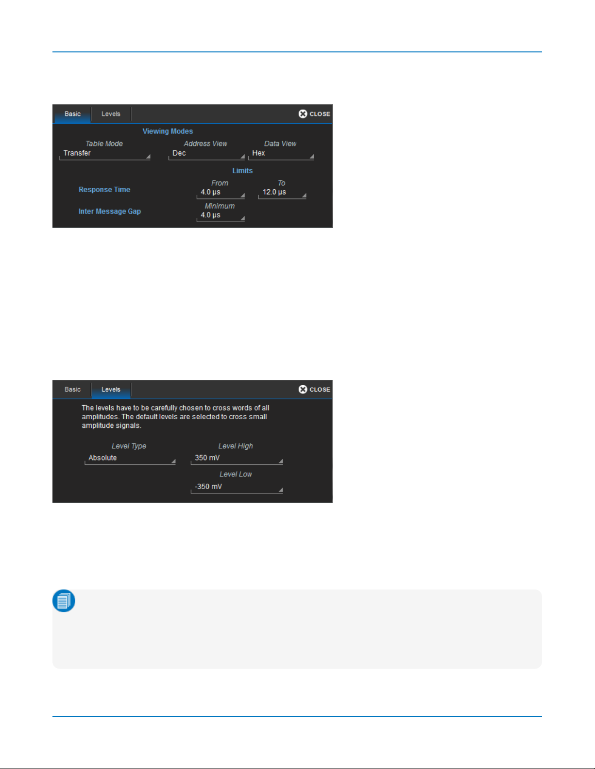
Basic Subdialog

Choose a Table Mode to optimize the result table for decoding Words or Transfers. Transfers adds columns
for Resp(onse), Data, and IMG bits.

Select to view Address bits in Decimal or Hex(adecimal) format.

Select to view Data bits in Decimal, Hex(adecimal), or Binary format.

Enter the Response Time Limits in From and To.

Enter the Inter Message Gap Miminum time.

Levels Subdialog

Enter the vertical Level High and Level Low used to determine the edge crossings of the MIL-STD-1553
signal. This value will be used to determine the bit-level decoding. Level is normally set as a percentage of
amplitude, and defaults to 50%. It can alternatively be set as an absolute voltage by changing the Level
Type to absolute. If your initial decoding indicates that there are a number of error frames, make sure that
the level is set to a reasonable value.

Note: Choose High and Low values carefully, as they are applied across all amplitudes. For
example: a transaction contains 20 V amplitude on the bus controller word and 2 V on the remote
terminal reply words, a ratio of 10:2. The level has to be adjusted to decode the lowest amplitude
words (2 V) with a gain of, say, 1 V/div and the high amplitude words (20 V), which are overflow but
are still decoded.

7

Find Quality Products Online at: [e-mail]

www.GlobalTestSupply.com

Avionics Protocols TDME Instruction Manual

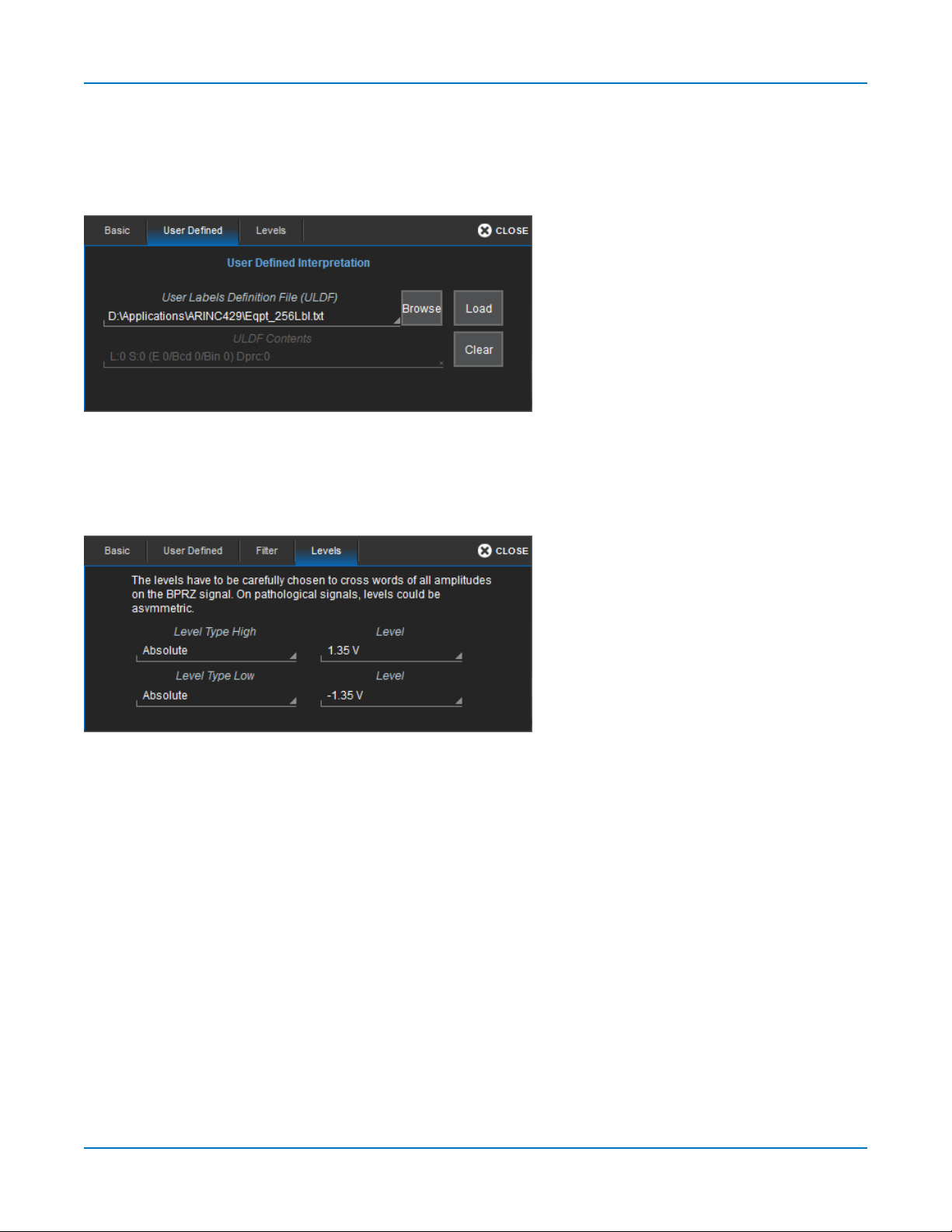
ARINC-429 Decoder Settings

Basic Subdialog

Enter the Bitrate of the bus to which you are connected as precisely as you know it. The value should be
correct within 5%. A mismatched bit rate will cause various confusing side effects on the decoding, so it is
best to take time to correctly adjust this fundamental value.

Under Viewing Control (viewing mode), select the Word format to apply: 8+24, 8+2+19+2+1, or User
Defined in a custom label file. See Label File Format for instructions on preparing the file. Go to the User
Defined tab to load the file.

In Viewing, choose to view/enter bits in Binary, Hex(adecimal), or Decimal format.

Check Details to see a Label's octal digits annotated (in all viewing modes). In 8+24 viewing mode, you will
also see the grouping of bits into digits. BCD digits are marked on the decoded waveform, showing the
correlation between the bit states and the n-bit BCD value.

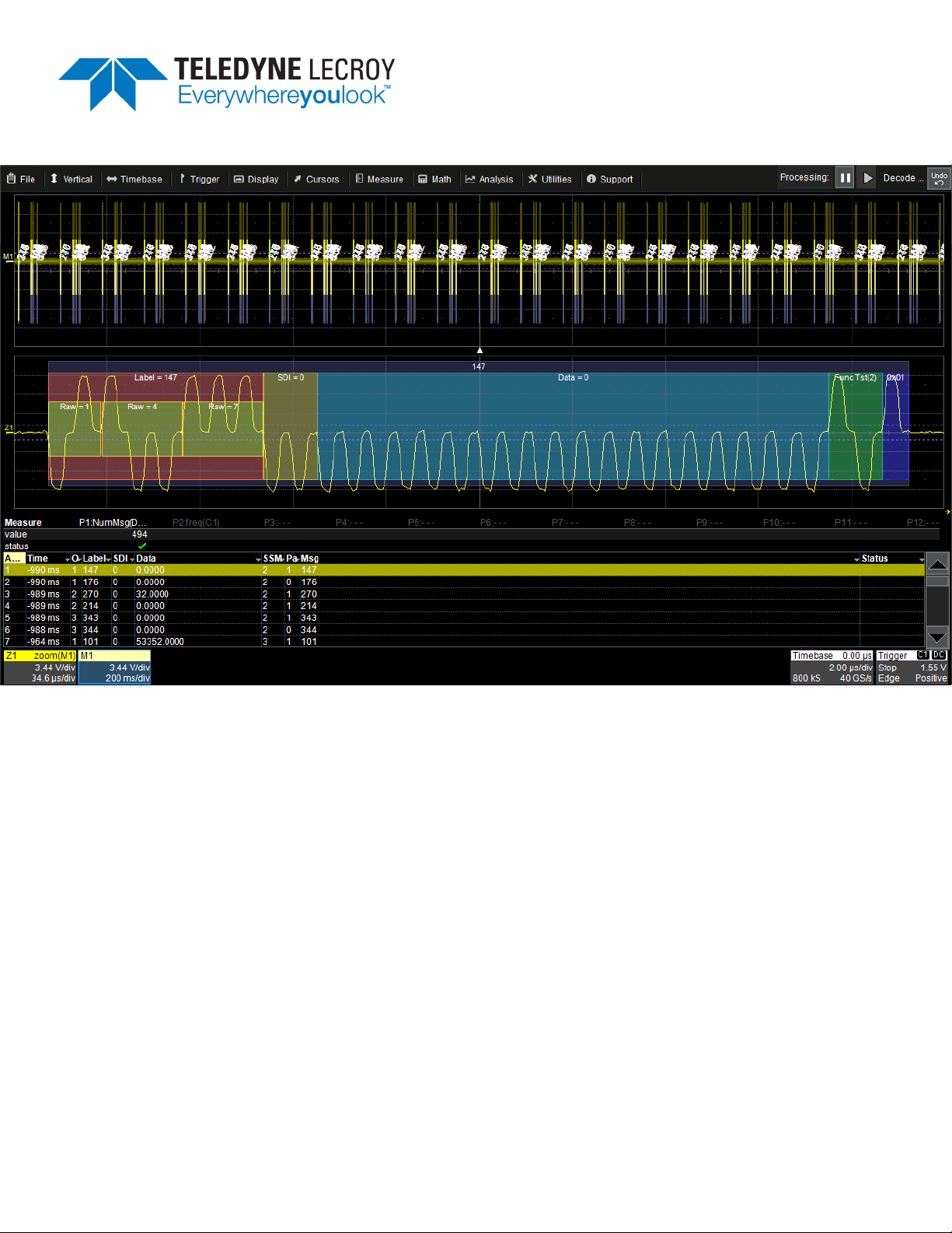
Note: In the example above, the Label digits are interpreted using the most significant bit first,
whereas the Data digits are interpreted least significant bit first.

8

Find Quality Products Online at: [e-mail]

www.GlobalTestSupply.com

Serial Decode

User Defined Subdialog

If you have chosen to use a custom symbolic label file, Browse to the file, then touch Load on the User
Defined subdialog.

Touch Clear to remove labels loaded from the previous file before choosing a new file.

Levels Subdialog

Enter the high and low voltage Level(s) that will cross words of all amplitudes on the BPRZ signal. Level is
usually set as a percentage of amplitude but may alternatively be set as an absolute voltage value by
changing the Level Type setting.

9

Find Quality Products Online at: [e-mail]

www.GlobalTestSupply.com

Avionics Protocols TDME Instruction Manual

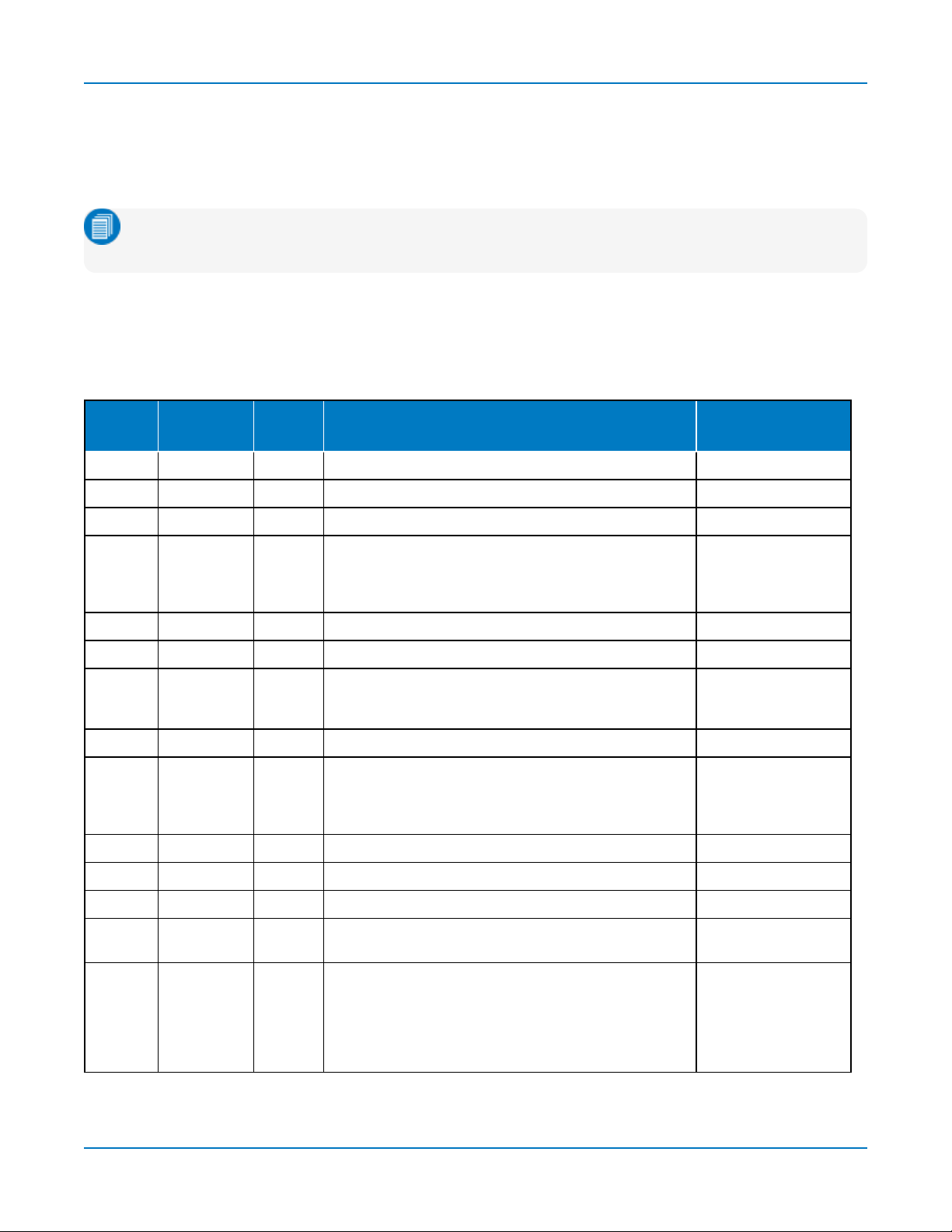
Label File Format

Label files (ULDF files) are Comma Separated Value (CSV) files containing the following tokens in the order
shown. You can use any neutral text editor to create/modify your Label file, as long as it does not add
extraneous characters or remove characters.

Note: All unused tokens must be present to correctly parse the line. However, unused tokens can be
left empty or contain a visual separator, such as "---" or “unused”.

ULDF files support commented lines starting with // as the normal C++ convention. Comments can also be
added at the end of the line, but not in the middle of the token list.

There is no limitation as to how many signals can be defined for a given label. Signals can be defined to be
overlapping, which is an error in most cases that is easily corrected by editing the SigBits and Offset Fields.

Position Field Name

1 Label Decimal 0 to 377, label in which the signal resides Yes

2 EquipmentID Text Free text No

3 Name Text Free text, name of the signal Yes

4 Units Text Free text Yes, for binaries

5 Min Text Free text No

6 Max Text Free text No

7 SigBits Decimal 1-32, number of bits spanned by the signal within the

8 PosSense Text Free text No

9 Resolution Decimal -max double to +max double Yes, for binaries

10 MinTransit Text Free text No

Content
Type

Range

ARINC word. SigBits and Offset define the position and
size of the annotation on the decoder overlay.

Used by Decoder
Algorithm?

(signed and
unsigned) and BCD
signals only

Yes, by all sub-types

(signed and
unsigned) and BCD
signals only

11 MaxTransit Text Free text No

12 LabelType1 Keyword Label_Discrete is the only usable value Yes

13 Offset Decimal 0-31, zero-based offset in bits from bit 0 at the beginning

of the message

14 DetailsList Special

format

SignedBinary, for example:
Enum: On|Off
Enum: Disengaged|Engaged
Enum: Off|Low|Medium|Full
BCD: 3|4
BCD: 2|4|4|4

Yes

Yes, additional inform­ation for BCD and
Enumerated Discretes

10

Find Quality Products Online at: [e-mail]

www.GlobalTestSupply.com

Serial Decode

Failure to Decode

Three conditions in particular may cause a decoder to fail, in which case a failure message will appear in the
first row of the summary result table, instead of in the message bar as usual.

All decoders will test for the condition Too small amplitude. If the signal’s amplitude is too small with respect
to the full ADC range, the message “Decrease V/Div” will appear. The required amplitude to allow decoding
is usually one vertical division.

If the decoder incorporates a user-defined bit rate (usually these are protocols that do not utilize a dedicated
clock/strobe line), the following two conditions are also tested:

l Under sampled. If the sampling rate (SR) is insufficient to resolve the signal adequately based on the

bit rate (BR) setup or clock frequency, the message "Under Sampled" will appear. The minimum
SR:BR ratio required is 4:1. It is suggested that you use a slightly higher SR:BR ratio if possible, and
use significantly higher SR:BR ratios if you want to also view perturbations or other anomalies on your
serial data analog signal.

l Too short acquisition. If the acquisition window is too short to allow any meaningful decoding, the

message “Too Short Acquisition” will appear. The minimum number of bits required varies from one
protocol to another, but is usually between 5 and 50.

In all the above cases, the decoding is turned off to protect you from incorrect data. Adjust your acquisition
settings accordingly, then re-enable the decoder.

Note: It is possible that several conditions are present, but you will only see the first relevant
message in the table. If you continue to experience failures, try adjusting the other settings.

Serial Decode Dialog

To first set up a decoder, go to the Decode Setup dialog. Once decoders have been configured, use the
Serial Decode dialog to quickly turn on/off a decoder or make minor modifications to the settings.

To turn on decoders:

1. On the same row as the Decode #, check On to enable the decoder.

As long as On is checked (and there is a valid acquisition), a result table and decoded waveform
appear. The number of rows of data displayed will depend on the Table #Rows setting (on the
Decode Setup dialog).

2. Optionally, modify the:

l Protocol associated with the decoder.

l Data (Source) to be decoded.

3. Check Link To Trigger On to tie this decoder setup to a serial trigger setup.

To turn off decoders: deselect the On boxes individually, or touch Turn All Off.

11

Find Quality Products Online at: [e-mail]

www.GlobalTestSupply.com

Avionics Protocols TDME Instruction Manual

Reading Waveform Annotations

When a decoder is enabled, an annotated waveform appears on the oscilloscope display, allowing you to
quickly see the relationship between the protocol decoding and the physical layer. A colored overlay marks
significant bit-sequences in the source signal: Header/ID, Address, Labels, Data Length Codes, Data,
CRC, Parity Bits, Start Bits, Stop Bits, Delimiters, Idle segments, etc. Annotations are customized to the
protocol or encoding scheme.

The amount of information shown on an annotation is affected by the width of the rectangles in the overlay,
which is determined by the magnification (scale) of the trace and the length of the acquisition. Zooming a
portion of the decoder trace will reveal the detailed annotations.

MIL-STD-1553 Waveform Annotations

Annotation Overlay Color (1) Text (2)

Message Charcoal (behind words) <transfer type>

Word Navy Blue (behind other fields) <type> Word

Sync Bits Grey Sync = <value>

RT Address and SubAddress Bits Brick Red RT Address = <value>

SubAddMode = <value>

Receive/Transmit Bit Purple < R | T >

Data Count Bits Green DataCount = <value>

Parity Bits Royal Blue <value>

Payload Data Bytes and
Single-bit Condition Codes

Reserved Bits Yellow Res = <value>

Response Time Check and
Inter-Message Gap

Protocol Error Bright Red (behind other fields) Error=<type>

1. Combined overlays affect the appearance of colors.

2. Text in brackets < > is variable. The amount of text shown depends on your zoom factors.

Aqua Blue Data = <value>

Teal # = <value>

** = <value>

Initial decoding. At this resolution, little information appears on the overlay.

Zoom of single index showing annotation details.

12

Find Quality Products Online at: [e-mail]

www.GlobalTestSupply.com

Word and Transfer Level Error Codes

Word and Transfer Level errors are indicated by a 3-character code on the overlay.

Note: Lowercase codes indicate Word errors, while uppercase codes indicate Transfer errors.

Code Error Type

par Parity word

ADD Add mismatch transfer

RTI Response time transfer

WCO Word count transfer

IMG Inter-message gap transfer

CTG Non-contiguous transfer

ARINC-429 Waveform Annotations

Annotation Overlay Color (1) Text (2) (3)

Frame ID Navy Blue (behind other fields) <value>

Serial Decode

Label Brick Red Label = <value>

Raw Bits Yellow (on top of Label) Raw = <value>

Source-Destination ID Olive Green SDI = <value>

Payload Data Aqua Blue Data = <value>

Functional Test and Failure Bright Green FuncTest = <value>

Fail (0)

Parity Bits Royal Blue <value>

Protocol Error Bright Red (behind other fields) Error=<type>

1. Combined overlays affect the appearance of colors.

2. Text in brackets < > is variable. The amount of text shown depends on your zoom factors.

3. Data values are shown in symbolic or hexadecimal depending on your decoder selection.

Initial decoding.

Zoom of single index showing annotation details.

13

Find Quality Products Online at: [e-mail]

www.GlobalTestSupply.com

Avionics Protocols TDME Instruction Manual

Serial Decode Result Table

When View Decode is checked on the Decode Setup Dialog

and

a source signal has been decoded using
that protocol, a table summarizing the decoder results appears below the grids. This result table provides a
view of data as decoded during the most recent acquisition, even when there are too many bursts for the
waveform annotation to be legible.

You can export result table data to a .CSV file. See also Automating the Decoder.

Tip: If any downstream processes such as measurements reference a decoder, the result table
does not have to be visible in order for the decoder to function. Hiding the table can improve
performance when your aim is to export data rather than view the decoding.

Table Rows

Each row of the table represents one index of data found within the acquisition, numbered sequentially.
Exactly what this represents depends on the protocol and how you have chosen to "packetize" the data
stream when configuring the decoder (frame, message, packet, etc.).

Note: For some decoders, it is even possible to turn off packetization, in which case
all the decoded data appears on one row of the table.

When multiple decoders are run at once, the index rows are combined in a summary table, ordered
according to their acquisition time. The Protocol column is colorized to match the input source that resulted
in that index.

You can change the number of rows displayed on the table at one time. The default is five rows.

Swipe the table up/down or use the scrollbar at the far right to navigate the table. See Using the Result

Table for more information about how to interact with the table rows to view the decoding.

Table Columns

When a single decoder is enabled, the result table shows the protocol-specific details of the decoding. This
detailed result table may be customized to show only selected columns.

A summary result table combining results from two decoders always shows these columns.

Column Extracted or Computed Data

Index Number of the line in the table

Time Time elapsed from start of acquisition to start of message

Protocol Protocol being decoded

Message Message identifier bits

Data Data payload

CRC Cyclic Redundancy Check sequence bits

Status Any decoder messages; content may vary by protocol

14

Find Quality Products Online at: [e-mail]

www.GlobalTestSupply.com

Serial Decode

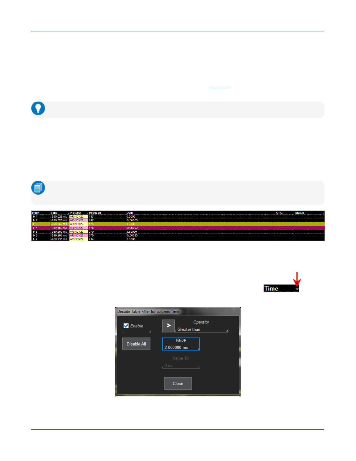
Example summary result table, with results from two decoders combined on one table.

When you select the Index number from the summary result table, the detailed results for that index drop-in
below it.

Example summary result table showing drop-in detailed result table.

ARINC-429 Result Table

Column Extracted or Computed Data

Index
(always shown)

Time Time elapsed from start of acquisition (trigger) to start of message frame

OctalDigits Octal Digits constituting the Label

Label Identifier showing data type and parameter association, typically shown as octal numbers

SDI Source-Destination Identifier

Data Data payload bits 11-29

SSM Sign-Status Matrix

Parity Value of the parity bit for this message

Msg Message Title derived from the ULDF file

Symbols Information contents of the message resulting from symbolic information in the ULDF file

Status Information regarding message errors, etc.

Number of the line in the table

Section of typical ARINC-429 detailed result table.

15

Find Quality Products Online at: [e-mail]

www.GlobalTestSupply.com

Avionics Protocols TDME Instruction Manual

MIL-STD-1553 Result Table

Note: Only a subset of these columns is shown in Word Table Mode.

Column Extracted or Computed Data

Index
(always shown)

Time Time elapsed from start of acquisition (trigger) to start of message

Type Word type (CW, DW, SW) or Transfer Type (see Mil 1553 specification for the list of 10

Summary Summary of the Transfer, with RT address(es) and number of Words or Mode Code,

Sync Sync Pulse Polarity

RTAddress Remote terminal address

t/r Transmit or Receive bit

SubAddress Location of data

Count Data count bit

ModeCode Mode Command code

ResponseTime Response latency of RT for all transfers using a handshake

RTAddressAck Remote terminal acknowledge code

MsgErr Message Error flag

Instr Instrumentation flag

SRQ Service Request flag

Number of the line in the table

Transfer Types), depending on the Table Mode

depending on the Transfer Type

Reserved Reserve bits (3)

BcastRec Broadcast command received

Busy Busy bit

SubSystFlg Sub-system flag

DynBusAcc Dynamic bus control accept

TermFlg Terminal flag

Data Data payload bytes

IMG Inter-Message Gap time

Status Information regarding message errors, etc.

Attributes Attribute flags

Section of typical MIL-STD-1553 detailed result table.

16

Find Quality Products Online at: [e-mail]

www.GlobalTestSupply.com

Serial Decode

Using the Result Table

Besides displaying the decoded serial data, the result table helps you to inspect the acquisition.

Zoom & Search

Touching any cell of the table opens a zoom centered around the part of the waveform corresponding to the
index. The Zndialog opens to allow you to rescale the zoom, or to Search the acquisition. This is a quick way
to navigate to events of interest in the acquisition.

Tip: When in a summary table, touch any data cell

The table rows corresponding to the zoomed area are highlighted, as is the zoomed area of the source
waveform. The highlight color reflects the zoom that it relates to (Z1 yellow, Z2 pink, etc.). As you adjust the
zoom scale, the highlighted area may expand to several rows of the table, or fade to indicate that only a part
of that Index is shown in the zoom.

When there are multiple decoders running, each can have its own zoom of the decoding highlighted on the
summary table at the same time.

Note: The zoom number is no longer tied to the decoder number. The software tries to match the
numbers, but if it cannot it uses the next zoom that is not yet turned on.

Example multi-decoder summary table, both zoomed indexes highlighted.

other than

Index and Protocol to zoom.

Filter Results

Those columns of data that have a drop-down arrow in the header cell can be filtered: Touch
the header cell to open the Decode Table Filter dialog.

Select a filter Operator and enter a Value that satisfies the filter condition.

17

Find Quality Products Online at: [e-mail]

www.GlobalTestSupply.com

Avionics Protocols TDME Instruction Manual

Operators Data Types Returns

=, ≠ Numeric or Text Exact matches only

>, ≥, <, ≤ Numeric All data that satisfies the operator

In Range, Out Range Numeric All data within/without range limits

Equals Any (on List),
Does Not Equal Any (on List)

Contains, Does Not Contain Text All data that contains or does not contain the string

Text All data that is/is not an exact match to any full value on

the list. Enter a comma-delimited list of values, no spaces
before or after the comma, although there may be spaces
within the strings.

Note: Once the Operator is selected, the dialog shows the format that may be entered in Value for
that column of data. Numeric values must be within .01% tolerance of a result to be considered a
match. Text values are case-sensitive, including spaces within the string.

Select Enable to turn on the column filter; deselect it to turn off the filter. Use the Disable All button to
quickly turn off multiple filters. The filter settings remain in place until changed and can be re-enabled on
subsequent decodings.

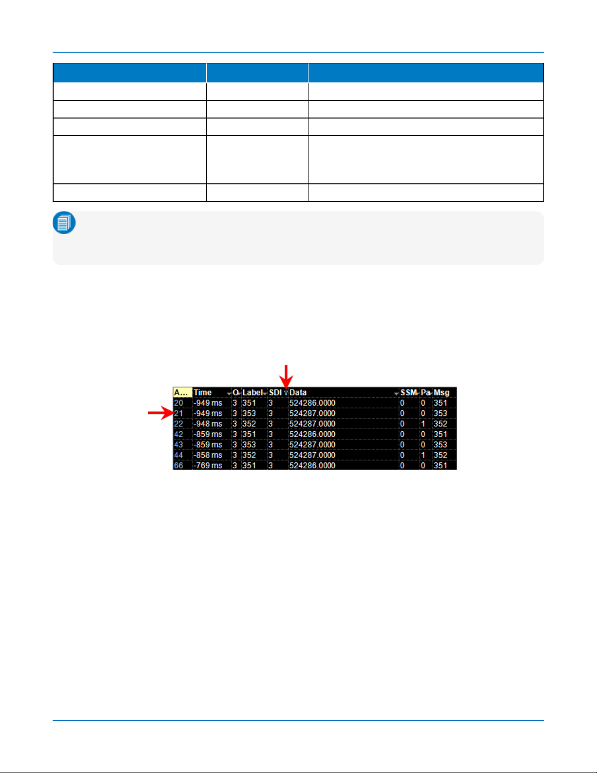
Those columns of data that have been filtered will have a funnel icon (similar to Excel) in the header cell, and
the index numbers will be colorized.

Example filtered decoder table.

On summary tables, only the Time, Protocol, and Status columns can be filtered.

If you apply filters to a single decoder table, the annotation is applied to only that portion of the waveform
corresponding to the filtered results, so you can quickly see where those results occurred. Annotations are
not affected when a summary table is filtered.

Also, eye diagrams are modified to represent only the filtered results, which can help to identify exactly
which indices of data are the cause of signal integrity problems.

View Details

When viewing a summary table, touch the Index number in the first column to drop-in the detailed decoding
of that record. Touch the Index cell again to hide the details.

If there is more data than can be displayed in a cell, the cell is marked with a white triangle in the lower-right
corner. Touch this to open a pop-up showing the full decoding.

18

Find Quality Products Online at: [e-mail]

www.GlobalTestSupply.com

Serial Decode

Navigate

In a single decoder table, touch the Index column header (top, left-most cell of the table) to open the
Decode Setup dialog. This is especially helpful for adjusting the decoder during initial tuning.

When in a summary table, the Index column header cell opens the Serial Decode dialog, where you can
enable/disable all the decoders. Touch the Protocol cell to open the Decode Setup dialog for the decoder
that produced that index of data.

19

Find Quality Products Online at: [e-mail]

www.GlobalTestSupply.com

Avionics Protocols TDME Instruction Manual

Customizing the Result Table

Performance may be enhanced if you reduce the number of columns in the result table to only those you
need to see. It is also especially helpful if you plan to export the data.

1. Press the Front Panel Serial Decode button or choose Analysis > Serial Decode, then open the
Decode Setup tab.

2. Touch the Configure Table button.

3. On the View Columns pop-up dialog, mark the columns you want to appear and clear those you
wish to remove. Only those columns selected will appear on the oscilloscope display.

Note: If a column is not relevant to the decoder as configured, it will not appear.

To return to the preset display, touch Default.

4. Touch the Close button when finished.

On some decoders, you may also use the View Columns pop-up to set a Bit Rate Tolerance percentage.
When implemented, the tolerance is used to flag out-of-tolerance messages (messages outside the user­defined bitrate +- tolerance) by colorizing in red the Bitrate shown in the table.

You may customize the size of the result table by changing the Table # Rows setting on the Decode Setup
dialog. Keep in mind that the deeper the table, the more compressed the waveform display on the grid,
especially if there are also measurements turned on.

Exporting Result Table Data

You can manually export the detailed result table data to a .CSV file:

1. Press the Front Panel Serial Decode button, or choose Analysis > Serial Decode, then open the
Decode Setup tab.

2. Optionally, touch Browse and enter a new File Name and output folder.

3. Touch the Export Table button.

Export files are by default created in the D:\Applications\<protocol> folder, although you can choose any
other folder on the oscilloscope or any external drive connected to a host USB port. The data will overwrite
the last export file saved, unless you enter a new filename.

Note: Only rows and columns displayed are exported. When a summary table is exported, a
combined file is saved in D:\Applications\Serial Decode. Separate files for each decoder are saved
in D:\Applications\<protocol>.

The Save Table feature will automatically create tabular data files with each acquisition trigger. The file
names are automatically incremented so that data is not lost. Choose File > Save Table from the
oscilloscope menu bar and select Decodexas the source.

20

Find Quality Products Online at: [e-mail]

www.GlobalTestSupply.com

Serial Decode

Using MsgToValue

MsgToValue enables you to apply oscilloscope features to a subset of the result table and is aimed at
protocols with addressed packets containing varying types of data, like CAN, LIN, MIL1553 and many
others. With it, you can filter the table by a particular ID to extract and convert decoded data values into a
parameter that can be used for other math or measurement processing.

MsgToValue requires several selections from the parameter set up subdialogs:

l Choose whether or not you wish to Filter by ID or accept Any packets.

l If you are filtering by ID, enter the desired ID on the ID subdialog.

l On the Value subdialog, enter the Data to Extract and any Conversion to be made.

Follow these steps to define the values to extract:

1. SYMBOLIC users: touch Browse DBC. Expand the .dbc file, then click on the desired symbol to filter
on occurrences of that symbol.

Note: This button will not appear if your installation does not support symbolic decoding.

2. Under Data to Extract, begin by entering the Start position and the # Bits to extract.

3. Choose the Encoding type if the signal uses encoding, otherwise leave it Unsigned.

4. Under Conversion, enter the a. Coefficient and b. Term that satisfy the formula:

Value = Coefficient * Raw Value + Term

.

5. Optionally, enter a Unit for the extracted decimal value.

21

Find Quality Products Online at: [e-mail]

www.GlobalTestSupply.com

Avionics Protocols TDME Instruction Manual

Searching Decoded Waveforms

Touching the Action toolbar Search button button on the Decode Setup dialog creates a 10:1 zoom of the
center of the decoder source trace and opens the Search subdialog.

Touching the any cell of the result table similarly creates a zoom and opens Search, but of only that part of
the waveform corresponding to the index (plus any padding).

Tip: In summary table mode, touch any cell

other than

Index and Protocol to create the zoom.

Basic Search

On the Search subdialog, select what type of data element to Search for. These basic criteria vary by
protocol, but generally correspond to the columns of data displayed on the detailed decoder result table.

Optionally:

l Check Use Value and enter the Value to find in that column. If you do not enter a Value, Search goes

to the beginning of the next data element of that type found in the acquisition.

l Enter a Left/Right Pad, the percentage of horizontal division around matching data to display on the

zoom.

l Check Show Frame to mark on the overlay the frame in which the event was found.

After entering the Search criteria, use the Prev and Next buttons to navigate to the matching data in the
table, simultaneously shifting the zoom to the portion of the waveform that corresponds to the match.

The touch screen message bar shows details about the table row and column where the matching data was
found.

Advanced Search

Advanced Search allows you to create complex criteria by using Boolean AND/OR logic to combine up-to­three different searches. On the Advanced dialog, choose the Col(umns) to Search 1 - 3 and the Value to
find just as you would a basic search, then choose the Operator(s) that represent the relationship between
them.

22

Find Quality Products Online at: [e-mail]

www.GlobalTestSupply.com

Serial Decode

Decoding in Sequence Mode

Not supported on WaveSurfer3000 and WaveSurfer 3000z models.

Decoders can be applied to Sequence Mode acquisitions. In this case, the index numbers on the result table
are followed by the segment in which the index was found and the number of the sample within that
segment:

index(segment-sample

Note: For some protocols, the Serial Trigger does not support Sequence Mode acquisitions,
although you could still decode Sequence Mode acquisitions made using a different trigger type.

Example filtered result table for a sequence mode acquisition.

).

In the example above, each segment was triggered on the occurrence of ID 0x400, which occurred only
once per segment, so there is only one sample per segment. The Time shown for each index in a Sequence
acquisition is absolute time from the first segment trigger to the beginning of the sample segment.

Otherwise, the results are the same as for other types of acquisitions and can be zoomed, filtered, searched,
or used to navigate. When a Sequence Mode table is filtered, the waveform annotation appears on only
those segments and samples corresponding to the filtered results.

Note: Waveform annotations can only be shown when the Sequence Display Mode is Adjacent.
Annotations are not adjusted when a Sequence Mode summary table is filtered, only the table data.

Multiple decoders can be run on Sequence Mode acquisitions, but in a summary table, each decoder will
have a first segment, second segment, etc., and there may be any number of samples in each. As in any
summary table, the samples will be interleaved and indexed according to their actual acquisition time. So,
you may find (3-2) of one decoder before (1-1) of another. Filter on the Protocol column to see the
sequential results for only one decoder.

23

Find Quality Products Online at: [e-mail]

www.GlobalTestSupply.com

Avionics Protocols TDME Instruction Manual

Improving Decoder Performance

Digital oscilloscopes repeatedly capture "windows in time". Between captures, the oscilloscope is
processing the previous acquisition.

The following suggestions can improve decoder performance and enable you to better exploit the long
memories of Teledyne LeCroy oscilloscopes.

Where possible, decode Sequence Mode acquisitions. By using Sequence mode, you can take many
shorter acquisitions over a longer period of time, so that memory is targeted on events of interest.

Note: For some protocols, the Serial Trigger does not support Sequence Mode acquisitions,
although you could still decode Sequence Mode acquisitions made using a different trigger type.

Parallel test using multiple oscilloscope channels. Up-to-four decoders can run simultaneously, each
using different data or clock input sources. This approach is statistically interesting because multi-channel
acquisitions occur in parallel. The processing is serialized, but the decoding of each input only requires 20%
additional time, which can lessen overall time for production validation testing, etc.

Avoid oversampling. Too many samples slow the processing chain.

Optimize for analysis, not display. The oscilloscope has a preference setting (Utilities > Preference Setup
> Preferences) to control how CPU time is allocated. If you are primarily concerned with quickly processing
data for export to other systems (such as Automated Test Equipment) rather than viewing it personally, it
can help to switch the Optimize For: setting to Analysis.

Turn off tables, annotations, and waveform traces. As long as downstream processes such as
measurements or Pass/Fail tests reference a decoder, the decoder can function without actually displaying
results. If you do not need to see the results but only need the exported data, you can deselect View
Decode, or minimize the number of lines in a table. Closing input traces also helps.

Decrease the number of columns in tables. Only the result table rows and columns shown are exported. It
is best to reduce tables to only the essential columns if the data is to be exported, as export time is
proportional to the amount of data exchanged.

24

Find Quality Products Online at: [e-mail]

www.GlobalTestSupply.com

Serial Decode

Automating the Decoder

As with all other oscilloscope settings, decoder features such as result table configuration and export can be
configured remotely.

Configuring the Decoder

The object path to the decoder Control Variables (CVARs) is:

app.SerialDecode.Decode

Wherenis the decoder number, 1 to 4. All relevant decoder objects will be nested under this. Use the
XStreamBrowser utility (installed on the oscilloscope desktop) to view the entire object hierarchy.

The CVAR app.SerialDecode.Decoden.Decode.ColumnState contains a pipe-delimited list of all the table
columns that are selected for display. For example:

app.SerialDecode.Decode1.Decode.ColumnState = "Idx=On|Time=On|Data=On|..."

If you wish to hide or display columns, send the full string with the state changed from "on" to "off", or vice
versa, rather than remove any column from the list.

Timebase, Trigger, and input Channel objects are found under app.Acquisition.

n

Accessing the Result Table

The data in the decoder Result Table can be accessed using the Automation object:

app.SerialDecode.Decoden.Out.Result.CellValue(

n

:= 1 to 4

line index

:= 1 to K

line index,column index)(item index,depth index

)

column index

item index

depth index

:= {0, 1, 2} where 0=Value, 1=StartTime, 2=StopTime

:= 1 to L

:= 1 to M

25

Find Quality Products Online at: [e-mail]

www.GlobalTestSupply.com

Serial Trigger

Serial Trigger

TD options provide advanced serial data triggering in addition to decoding. Serial data triggering is
implemented directly within the hardware of the oscilloscope acquisition system. The serial data trigger
scrutinizes the data stream in real time to recognize "on-the-fly" the user-defined serial data conditions.
When the desired pattern is recognized, the oscilloscope takes a real-time acquisition of all input signals as
configured in the instrument's acquisition settings. This allows decode and analysis of the signal being
triggered on, as well as concomitant data streams and analog signals.

The serial trigger supports fairly simple conditions, such as "trigger at the beginning of any packet," but the
conditions can be made more restrictive depending on the protocol and the available filters, such as "trigger
on packets with ID = 0x456". The most complex triggers incorporate a double condition on the ID and data,
for example "trigger on packets with ID = 0x456 and when data in position 27 exceeds 1000".

Note: The trigger and decode systems are independent, although they are seamlessly coordinated
in the user interface and the architecture. It is therefore possible to use the serial trigger without
decoding the acquisition, or to decode acquisitions made without using the serial trigger.

Note: These instructions pertain only to the -TD and -TDME options for those protocols and
encoding schemes where serial trigger is supported: 8b10b, 64b66b, 80-bit NRZ, MIL-1553,
AudioBus (I2S/RJ/LJ), I2C, I3C, SPI, UART-RS232, CAN, CAN FD, LIN, FlexRay, SATA, SPMI,
and USB2.

Requirements

Serial trigger options require the appropriate hardware (please consult support), an installed option key, and
the latest firmware release.

Restrictions

The serial trigger only operates on one protocol at a time. It is therefore impossible to express a condition
such as "trigger on CAN frames with ID = 0x456 followed by LIN packet with Adress 0xEBC."

Linking Trigger and Decoder

A quick way to set up a serial trigger is to link it to a decoder by checking the Link to Trigger ("On") box on
the Serial Decode dialog. Linking trigger and decoder allows you to configure the trigger with the exact same
values that are used for decoding the signal (in particular the bit rate), saving the extra effort needed to re­enter values on the serial trigger set up dialogs.

While the decoder and the trigger have distinct sets of controls, when the link is active, a change to the bit
rate in the decoder will immediately propagate to the trigger and vice-versa.

27

Find Quality Products Online at: [e-mail]

www.GlobalTestSupply.com

Avionics Protocols TDME Instruction Manual

MIL-STD-1553 Trigger Setup

To access the serial trigger dialogs:

l Touch the Trigger descriptor box or choose Trigger > Trigger Setup from the Menu Bar.

l Touch the Serial Type button, and the MIL 1553 Standard button.

Then, working from left to right, make the desired selections from the MIL1553 dialog.

Source Setup

Select the DATA source channel.

Adjust the vertical level Threshold High and Low. MIL-STD-1553 is a tri-level signal and requires two
voltage threshold settings to enable the oscilloscope to distinguish between 1 and 0. If you've linked this
trigger to a MIL-STD-1553 decoder, these values are initially pulled from that setup.

Type

Choose one of the major trigger types of Transfer, Word, Error, or Timing.

The remaining options on the dialog will change to offer different trigger sub-types and condition settings.
Because these options vary significantly, the remainder of this section will describe each trigger type
separately.

Timing Trigger

Timing triggers can be set on the sub-type of either Response Time or Inter-Message Gap time.

On the subdialog, set the timing condition upon which to trigger.

Error Trigger

The oscilloscope can be set to trigger on finding a various types of MIL-STD-1553 protocol errors. Just
check all desired error types on the Errors subdialog.

28

Find Quality Products Online at: [e-mail]

www.GlobalTestSupply.com

Serial Trigger

Word Trigger

Word triggers upon finding a match to the trigger conditions in Command, Data, or Status Word frames.
The All sub-type will trigger upon the start of any Word.

Under Setup Format, choose to enter the Word conditions in either Binary or Hex(adecimal) format.

Note: In all condition statements, "X" may be used as a wild card in place of bit values where you
don't care what value appears.

Command Word Trigger

On the Command subdialog:

l Create condition statements describing the RT Address(es) and/or Sub Address(es) that will be

examined by the trigger. If you don't care about addresses, enter the condition "= XX".

l Create a condition statement describing the Command Mode Code upon which to trigger. For

example, entering "= 0" triggers upon finding Mode Code 0, Dynamic Bus Control, whereas entering
"> 2" triggers upon finding any code number higher than Mode Code 2, Transmit Status Word.

Data Word Trigger

On the Data subdialog, create a condition statement describing the data pattern upon which to trigger. The
data pattern can be further refined by defining a window, with the Start Bit and #Data Bits.

29

Find Quality Products Online at: [e-mail]

www.GlobalTestSupply.com

Avionics Protocols TDME Instruction Manual

Status Word Trigger

On the Status subdialog:

l Create a condition statement describing the RT Address(es) that will be examined by the trigger.

l For each of the Status Word bits, enter the value upon which to trigger. Leave X where you "don't

care" what the value is.

Transfer Triggers

Transfer triggers allow you to set complex conditions upon any combination of Command, Data, or Status
Words that may occur during one of the MIL-STD-1553 Transfer types. (It is assumed here that you are
familiar with the Transfer types specified by MIL-STD-1553B.)

First, choose trigger type Transfer and the Transfer Type. A list of possible combinations (e.g., BC-RT
(Rcv), Mode Command) appear on the Transfer Type pop-up menu.

Transfer Types

The possible trigger conditions are presented on subdialogs according to the structure of the transfer. For
example, if the selected Transfer has only one type of Word, only one corresponding Word subdialog will
appear for entering the trigger condition. Conversely, if the Transfer has a structure with a Command Word
and a Data Word, two subdialogs will appear. The logical binding is an AND condition. The trigger occurs
when both the condition described on dialog 1 AND the condition on dialog 2 are met on the same Transfer.
This logic extends to whatever number of conditions are specified.

Refer to the Command, Data, and Status Word Trigger procedures above for instructions on using each
type of dialog to create a condition statement.

All Triggers on any Transfer Type, without exercising

conditions on the contents.

BC–RT
(Rcv)

RT–BC
(Xmit)

RT–RT

Cmd Mode Command

30

Find Quality Products Online at: [e-mail]

www.GlobalTestSupply.com

Serial Trigger

Cmd
(Xmit)

Cmd
(Rcv)

BC–RT
(S)

RT–RT(S) Mode Command with Data Broadcast

Cmd(S) Mode Command Broadcast

Cmd(S)
(Rcv)

Mode Command with Data from RT

Mode Command with Data to RT

Mode Command with Data Broadcast

Mode Command with Data Broadcast

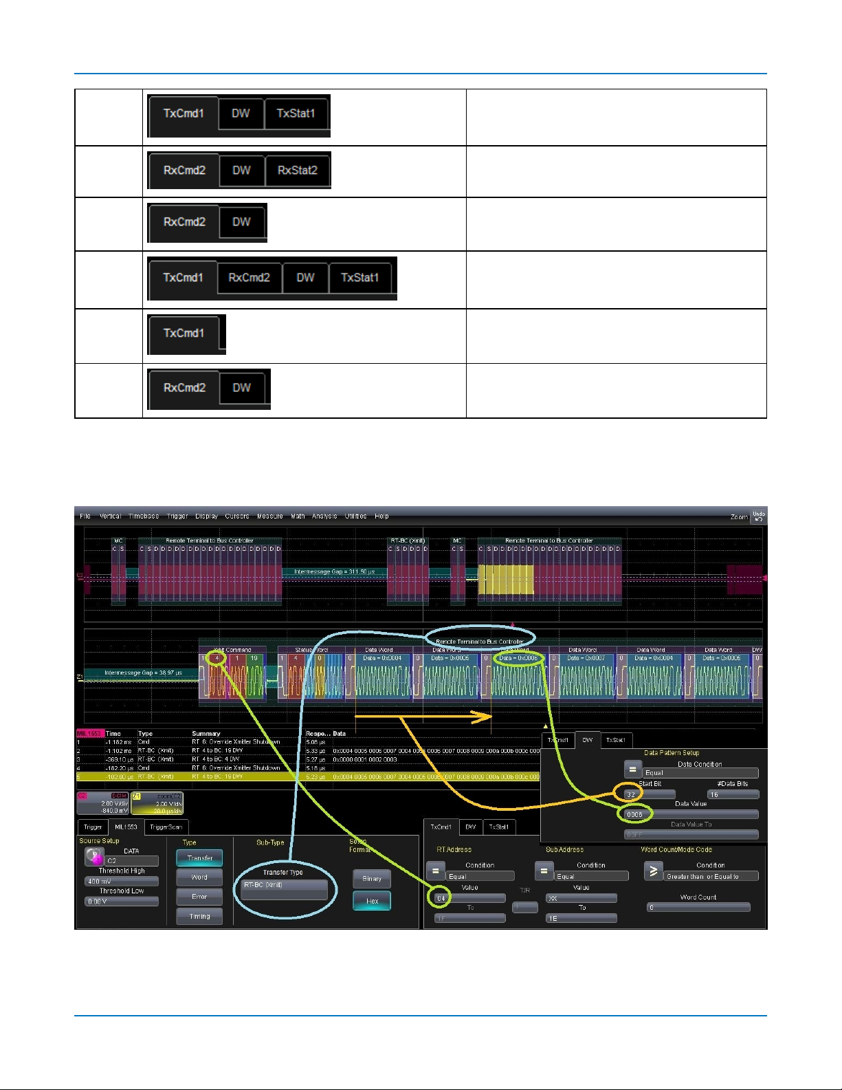
Example 1: Triggering on an RT–BC Transfer

The image below is a composite of trigger setup dialogs. The set of right-hand subdialogs matches the
selected Transfer Type of RT to BC: 1 TxCmd, 1 Data and 1 TxStatus.

The condition specifies that a trigger should occur when RT address=4 AND Data Word is position 32 =

0006. This exact event has been detected where the trigger position indicators (small pink and yellow

31

Find Quality Products Online at: [e-mail]

www.GlobalTestSupply.com

Avionics Protocols TDME Instruction Manual

triangles) appear on the waveform decoding. Note that the trigger position indicator is placed chronologically

after

the occurrence of DW=0006. This reflects the fact that the trigger, if it occurs, can only be emitted after

all the conditions have been met.

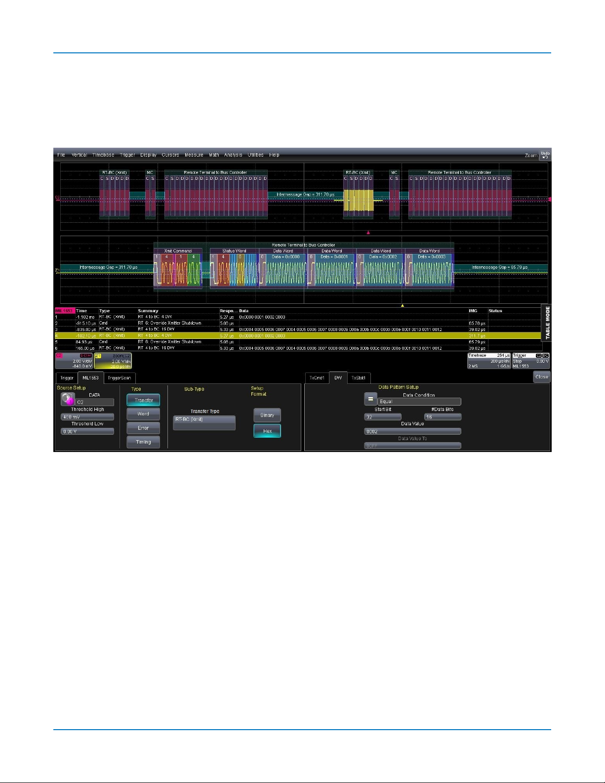
The following image shows the trigger that would occur if the Data Word condition were changed so that the
DW value was 0002 instead of 0006.

This trigger occurs on the same Transfer Type (RT–BC) for the same RT Address (RT=4) at the same Bit
Offset (32), but for a DW Value of 0002. The trigger position indicator is now observed after DW = 0002,
which in fact lies in another Transfer (the zoom Z1 is positioned differently on C2 then it was in the first
image).

32

Find Quality Products Online at: [e-mail]

www.GlobalTestSupply.com

Example 2: Triggering on a Mode Command

These images show a Transfer Type trigger set on a Mode Command transfer.

Serial Trigger

Trigger catches the Mode Command “Override Transmitter Shutdown”. The trigger time indicator and the decoder

overlay show this is the fourth Transfer in the stream captured on C2. The Mode Command translation appears in the

Summary column of the result table.

33

Find Quality Products Online at: [e-mail]

www.GlobalTestSupply.com

Avionics Protocols TDME Instruction Manual

Trigger catches the Mode Command “Dynamic Bus Control”. This is the third Transfer in the stream captured on C2.

34

Find Quality Products Online at: [e-mail]

www.GlobalTestSupply.com

Serial Trigger

Using the Decoder with the Trigger

A key feature of Teledyne LeCroy trigger and decode options is the integration of the decoder functionality
with the trigger. While you may not be interested in the decoded data per se, using the decoded waveform
can help with understanding and tuning the trigger.

Stop and Look

Decoding with repetitive triggers can be very dynamic. Stop the acquisition and use the decoder tools such
as Search, or oscilloscope tools such as TriggerScan, to inspect the waveform for events of interest. Touch
and drag the paused trace to show time pre- or post-trigger.

Optimize the Grid

The initial decoding may be very compressed and impossible to read. Try the following:

l Increase the height of the trace by

decreasing

the gain setting (V/Div) of the decoder source channel.

This causes the trace to occupy more of the available grid.

l Change your Display settings to turn off unnecessary grids. The Auto Grid feature automatically closes

unused grids. On many oscilloscopes, you can manually move traces to consolidate grids.

l Close setup dialogs.

Use Zoom

The default trigger point is at zero (center), marked by a small triangle of the same color as the input channel
at the bottom of the grid. Zoom small areas around the trigger point. The zoom will automatically expand to
fit the width of the screen on a new grid. This will help you to see that your trigger is occurring on the bits you
specified.

If you drag a trace too far left or right of the trigger point, the message decoding may disappear from the grid.
You can prevent "losing" the decode by creating a zoom of whatever portion of the decode interests you.
The zoom trace will not disappear when dragged and will show much more detail.

35

Find Quality Products Online at: [e-mail]

www.GlobalTestSupply.com

Avionics Protocols TDME Instruction Manual

Saving Trigger Data

The message decoding and the result table are dynamic and will continue to change as long as there are
new trigger events. As there may be many trigger events in long acquisitions or repetitive waveforms, it can
be difficult (if not impossible) to actually read the results on screen unless you stop the acquisition. You can
preserve data concurrent with the trigger by using the AutoSave feature.

l AutoSave Waveform creates a .trc file that copies the waveform at each trigger point. These files can

be recalled to the oscilloscope for later viewing. Choose File > Save Waveform and an Auto Save
setting of Wrap (overwrite when drive full) or Fill (stop when drive full). The files are saved in
D:\Waveforms.

l AutoSave Table creates a .csv file of the result table data at each trigger point. Choose File > Save

Table and an Auto Save setting of Wrap or Fill. The files are saved in D:\Tables.

Caution: If you have frequent triggers, it is possible you will eventually run out of hard drive space.
Choose Wrap only if you're not concerned about files persisting on the instrument. If you choose Fill,
plan to periodically delete or move files out of the directory.

36

Find Quality Products Online at: [e-mail]

www.GlobalTestSupply.com

Measure/Graph

Measure/Graph

The installation of the Measure/Graph package (included with any -DME or -TDME option) adds a set of
measurements and plots designed for serial data analysis to the oscilloscope's standard measurement
capabilities. Measurements can be quickly applied without having to leave the waveform or tabular views of
the decoding.

Note: This functionality was formerly offered as part of -TDM options and the ProtoBus MAG
software option. The features described in this section should be present If you have either of these
installed on your oscilloscope.

Serial Data Measurements

These measurements designed for debugging serial data streams can be applied to the decoded waveform.
Measurements appear in a tabular readout below the grid (the same as for any other measurements) and
are in addition to the result table that shows the decoded data. You can set up as many measurements as
your oscilloscope has parameter locations.

Note: Measurements appear in the Serial Decode sub-menu of the Measure Setup menu and may
have slightly different names. For example, the CAN sub-menu has measurements for CANtoValue
instead of MsgToValue, etc. The measurements are the same.

Measurement Filters Description

AnalogToMsg ID, Data, Analog Computes time from crossing threshold on an analog signal to start of first

message that meets conditions. If the message condition precedes the ana­log condition, no measurement is performed.

BusLoad ID, Data Computes the load of selected messages on the bus (as a percent).

DeltaMsg ID, Data Computes time difference between two messages on a single decoded line.

MsgBitrate ID, Data Computes the bitrate of selected messages within the decoded stream.

MsgToAnalog ID, Data, Analog Computes time from start of first message that meets conditions to crossing

threshold on an analog signal. If the analog condition precedes the mes­sage condition, no measurement is performed.

MsgToMsg ID, Data Computes time from start of first message that meets conditions to start of

the next message that meets conditions.

MsgToValue ID, Value Extracts a selected portion of the data to a measurement parameter loc-

ation, with optional conversion of value. Data may be selected by ID and/or
data field position.

NumMessages ID, Data Computes the total number of messages in the decoding that meet con-

ditions.

Time@Msg ID, Data Computes time from trigger to start of each message that meets conditions.

37

Find Quality Products Online at: [e-mail]

www.GlobalTestSupply.com

Avionics Protocols TDME Instruction Manual

Graphing Measurements

The Measure/Graph package include simplified methods for plotting measurement values as:

l Histogram - a bar chart of the number of data points that fall into statistically significant intervals or

bins. Bar height relates to the frequency at which data points fall into each interval/bin. Histogram is
helpful to understand the modality of a parameter and to debug excessive variation.

l Trend - a plot of the evolution of a parameter over time. The graph's vertical axis is the value of the

parameter; its horizontal axis is the order in which the values were acquired. Trending data can be
accumulated over many acquisitions. It is analogous to a chart recorder.

l Track - a time-correlated accumulation of values for a single acquisition. Tracks are time synchronous

and clear with each new acquisition. Track can be used to plot data values and compare them to a
corresponding analog signal, or to observe changes in timing. A parameter tracked over a long
acquisition could provide information about the modulation of the parameter.

These plots effectively perform a digital-to-analog conversion that can be viewed right next to the decoded
waveform.

To graph a measurement, just select the plot type from the Measure/Graph dialog when setting up the
measurement. All plots are created as Math functions that open along side the deocoding in a separate grid.

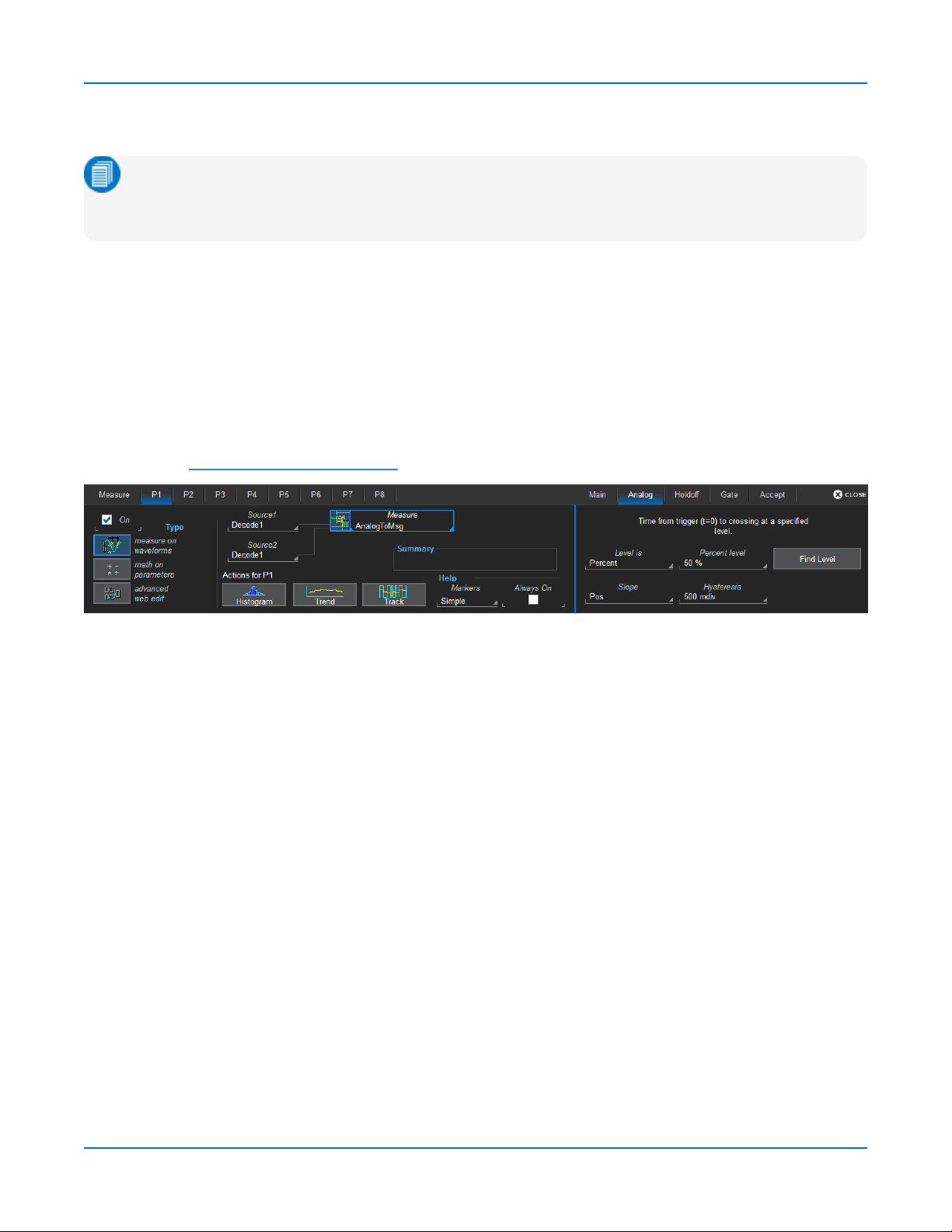
Measure/Graph Setup Dialog

Use the Measure/Graph Setup dialog to apply serial data measurement parameters to the decoded
waveform and simultaneously graph the results. This dialog appears behind the Decode Setup dialog and is
active when measurements are supported.

1. Select the Measurement to apply and the Destination parameter (Pn) to which to assign it.

2. The active decoder is preselected in Source 1, indicating the measurement will be applied to the
decoder results; change it if necessary. If the measurement requires it, also select an appropriate
Source 2 (such as an analog waveform for comparison).

3. Optionally:

l Touch Graph to select a plot type. Also select a Destination function (F

l Touch Apply & Configure to set a filter, gate or other qualifiers on the measurement.

n

) for the plot.

38

Find Quality Products Online at: [e-mail]

www.GlobalTestSupply.com

Measure/Graph

Filtering Measurements

Certain serial decode measurements can be filtered to include only the results from specified IDs or specific
data patterns. As with all measurements, you can set a gate to restrict measurements to a horizontal range
of the grid corresponding to a specific time segment of the acquisition.

After creating a measurement on the Measure/Graph Setup dialog, touch Apply&Configure. The touch
screen display will switch to the standard Measure setup dialogs for the parameter you selected. Set filter
conditions on the right-hand subdialogs that appear next to the Pndialogs.

ID Filter

This filter restricts the measurement to only frames/packets with a specific ID value. Settings on this dialog
may change depending on the protocol.

1. On the Main subdialog, choose to Filter by ID or ID + Data.

2. On the ID subdialog, choose to enter the ID in Binary or Hex(adecimal) format.

3. If the field appears, select the # Bits used to define the frame ID. (This will change the ID Value field
length.)

4. Using the ID Condition and ID Value controls, create a condition statement that describes the IDs
you want included in the measurement. To set a range of values, also enter the ID Value To.

Tip: On the value entry pop-up: use the arrow keys to position the cursor; use Back to clear
the previous character (like Backspace); use Clear to clear all characters.

Data Filter

This restricts measurements to only frames containing extracted data that matches the filter condition. It can
be combined with a Frame ID filter by choosing ID+Data on the Main subdialog.

Use the same procedure as above to create a condition describing the Data Value(s) to include in the
measurement. Use "X" as a wild card ("Don't Care") in any position where the value doesn't matter.

39

Find Quality Products Online at: [e-mail]

www.GlobalTestSupply.com

Avionics Protocols TDME Instruction Manual

Optionally, enter a Start Position within the data field byte to begin seeking the pattern, and the # Bits in the
data pattern. The remaining data fields positions will autofill with "X".

Note: For MsgtoMsg measurements, the data condition is entered twice: first for the Start Message
and then for the End Message. The measurement computes the time to find a match to each set of
conditions.

Analog Settings

The measurements AnalogToMsg and MsgToAnalog allow you to use crossing level and slope to define the
event in the Analog waveform that is to be used as the reference for the measurement.

As with the decoder, Level may be set as a percentage of amplitude (default), or as an absolute voltage level
by changing Level Is to Absolute. You can also use Find Level to allow the oscilloscope to set the level to
the mean Top-Base amplitude.

A Slope and Hysteresis selection is also offered. The width of the Hysteresis band is specified in milli­divisions. See Setting Level and Hysteresis for more information on using these controls.

40

Find Quality Products Online at: [e-mail]

www.GlobalTestSupply.com

Eye Diagram Tests

Eye Diagram Tests

The -DME and -TDME options provide easy eye diagram setup and eye mask testing.

Eye diagrams are a key component of serial data analysis. They are used both quantitatively and
qualitatively to understand the quality of the signal communications path. Signal integrity effects such as
intersymbol interference, loss, crosstalk and EMIcan be identified by viewing eye diagrams, such that the
eye is typically viewed prior to performing any further analysis.

Each pixel in the eye takes on a color that indicates how frequently a signal has passed through the time and
voltage specified for that pixel. The eye diagram shows all values a digital signal takes on during a bit period.
A bit period (also referred to as unit interval, or UI) is defined by the data clock, whether explicit or
extrapolated depending on the protocol.

Eye diagrams show the acquired signal that is currently being shown on the decoder result table. They are
not persistent, as are eye diagrams generated in some other serial data analysis software; the eye will
change from one acquisition to the next and when the result table is filtered. Our recommended approach for
using the eye diagrams is to:

l Make single shot acquisitions with decoder and eye diagram enabled to check that both are working

correctly.

l Run a normal acquisition with Mask Testing and Stop On Failure enabled in the Mask Failure Locator,

or with a Pass/Fail test set on one of the eye parameters.

Eye Diagram Setup Dialog

Create Eye Diagram

Open the Eye Diagram Setup dialog and select the Decode for which to create an eye diagram.

Under Eye, check Enable to display the eye diagram.

The Bitrate is automatically read from the decoder setup. This value is linked to the decoder bit rate setting,
and changing it in either place will update both settings.

The Upsample factor increases the number of sample points used to compose the eye diagram. Increase
from 1 to a higher number (e.g. 5) to fill in gaps. Gaps can occur when the bitrate is extremely close to a
submultiple of the sampling rate, such that the sampling of the waveform does not move throughout the
entire unit interval. Gaps can also occur when using a record length that does not sample a sufficiently large
number of unit intervals.

The Eye Style may utilize color-graded or analog persistence:

41

Find Quality Products Online at: [e-mail]

www.GlobalTestSupply.com

Avionics Protocols TDME Instruction Manual

l

With color-graded persistence , pixels are given a color based on the pixel's relative population
and the selected Eye Saturation. The color palette ranges from violet to red.

l

With analog persistence , the color used mimicks the relative intensity that would be seen on an
analog oscilloscope.

Use the Eye Saturation slider to adjust the color grading or intensity. Slide to the left to reduce the threshold
required to reach saturation.

Choose to display the Eye Height, Eye Width, or Mask Hit(s) measurement parameters. These are added
to the Measure table in the first open parameter slots.

Eye Mask Test

Under Mask, check Enable to turn on eye mask testing.

Select to use either a Standard or Custom mask, then either select the Standard Mask or Browse to and
select your custom Mask File.

Tip: Masks previously created on the instrument are stored in D:\Masks. For ease of selection, copy
other .msk files to this location.

Check Mask Failure On to mark the parts of the eye diagram that fail the mask test. Mask violations appear
as red failure indicators where the eye diagram intersects the mask.

Check Failure Location to display the Mask Failure Locator dialog.

Mask Failure Locator Dialog

Use this dialog to quickly search the acquisition for eye diagram mask test failures.

In Trace Width, enter the number of UIs surrounding the mask violation to display as "padding."

Check Stop On Failure to stop acquisition whenever an eye mask failure occurs.

Enter the Max Failures to retain in the Eye Mask Failure list.

Select from the Eye Mask Failure list to mark and zoom to the location of that failure. Yellow circles appear
over the red failure indicators to show the location of the failure.

42

Find Quality Products Online at: [e-mail]

www.GlobalTestSupply.com