Teledyne LeCroy HDO4054A-MS, HDO4034A-MS, HDO4024A-MS User manual

Operator's Manual

HDO4000 / HDO4000A
High Definition
Oscilloscopes

Find Quality Products Online at: [e-mail]

www.GlobalTestSupply.com

HDO4000/HDO4000A High Definition Oscilloscopes Operator's Manual

© 2021 Teledyne LeCroy, Inc. All rights reserved.

Users are permitted to duplicate and distribute Teledyne LeCroy, Inc. documentation for internal educational
purposes only. Resale or unauthorized duplication of Teledyne LeCroy publicationsis strictly prohibited.

Teledyne LeCroy is a trademark of Teledyne LeCroy, Inc., Inc. Other product or brand names are trademarks or
requested trademarks of their respective holders. Information in this publication supersedes all earlier versions.
Specificationsare subject to change without notice.

May, 2021
hdo4000a-om-eng_17may21.pdf

Find Quality Products Online at: [e-mail]

www.GlobalTestSupply.com

Contents

About This Manual iii

Oscilloscope Overview and Set Up 1

Safety 1
Overview 4
Powering On/Off 10
Software Activation 11
Language Selection 11
Connecting to Other Devices/Systems 11
Oscilloscope Application 12

Using MAUI 15

Touch Screen 15
MAUI with OneTouch 21
Controlling Traces 27
Zooming 32
Print/Screen Capture 34

Acquisition 35

Auto Setup 35
Vertical 36
Digital (Mixed Signal) 42
Timebase 46
Trigger 53

Display 63

Display Set Up 63
Persistence Display 65

Cursors 67

Cursor Types 67
Apply and Position Cursors 69
Standard CursorsDialog 70

Measure 71

Parameter Set Up 71
List of Standard Measurements 74
Measure Table 78
Using Trends 79

Math 81

Math Function Set Up 81
List of Standard Math Operators 83
Average Function 85
ERes Function 87
FFT Function 89
Rescale Function 91
Math Dialog 96

i

Find Quality Products Online at: [e-mail]

www.GlobalTestSupply.com

HDO4000/HDO4000A High Definition Oscilloscopes Operator's Manual

Memory 97

Saving Memories 97
Restoring Memories 98

Analysis Tools 99

WaveScan 99
PASS/FAIL Testing 103

Saving Data (File Functions) 105

Save 105
Trace File Format 111
Recall 114
LabNotebook 116
Report Generator 121
Share 122
Print 123
Email & Report Settings 124
Using the File Browser 125

Utilities 127

Utilities Dialog 127
Disk Utilities 132
Preferences Dialogs 133

Maintenance 139

Restart/Reboot Instrument 139
Restore Default Setup 139
Changing Screen Settings 139
Touch Screen Calibration 140
Windows 10 External Display Setup 140
Software and File Management 141
MAUI Firmware Update 142
Switching Windows Users 143
Technical Support 144
Returning a Product for Service 145

Index 147

ii

Find Quality Products Online at: [e-mail]

www.GlobalTestSupply.com

About This Manual

About This Manual

Thank you for purchasing a Teledyne LeCroy oscilloscope. We're certain you'll be pleased with the detailed
features unique to our instruments.

This manual shows the HDO4000A, although much of it could be applied to earlier instruments in the
series. With the introduction of later versionsof the 64-bit MAUI®software, particularly version 8.3 and
later, the graphical user interface on some instruments looked very different from what was offered on
earlier instruments and included different touch screen capabilities. Despite the difference in appearance,
however, the functionality is the same unlessotherwise stated. Where there are differences or limitations
in capabilities, these are explained in the text.

Our website maintainsthe most current product specifications and should be checked for updates.
Detailed specificationsare listed on the product datasheet.

Note: Specifications are subject to change without notice.

iii

Find Quality Products Online at: [e-mail]

www.GlobalTestSupply.com

HDO4000/HDO4000A High Definition Oscilloscopes Operator's Manual

iv

Find Quality Products Online at: [e-mail]

www.GlobalTestSupply.com

Oscilloscope Overview and Set Up

Oscilloscope Overview and Set Up

Safety

Symbols

These symbols appear on the instrument or in documentation to alert you to important safety concerns:

Caution of potential damage to instrument or Warning of potential bodily injury. Refer to
manual. Do not proceed untilthe information is fully understood and conditions are met.

Caution, high voltage; risk of electric shock or burn.

Caution

Frame or chassis terminal (ground connection).

Alternating current.

Standby power (front of instrument).

, contains parts/assemblies susceptible to damage by Electrostatic Discharge (ESD).

Precautions

Observe generally accepted safety procedures in addition to the precautions listed here. The overall
safety of any system incorporating this product isthe responsibility of the assembler of the system.

Use indoors only .

Use only within the operational environment listed. Do not use in wet or explosive atmospheres.

Maintain ground. The ACinlet ground is connected directly to the chassis of the . To avoid electric shock,
connect only to a mating outlet with a safety ground contact.

Caution: Interrupting the protective conductor inside or outside the oscilloscope, or disconnecting
the safety ground terminal, creates a hazardous situation. Intentional interruption is prohibited.

Connect and disconnect properly. Do not connect/disconnect probes, test leads, or cables while they are
connected to a live voltage source.

Observe all terminal ratings. Do not apply a voltage to any input that exceeds the maximum rating of that
input. Refer to the body of the instrument for maximum input ratings.

Use only the power cord shipped with and certified for the country of use.

Keep product surfaces clean and dry. See Cleaning.

Do not remove the covers or inside parts. Refer all maintenance to qualified service personnel.

Exercise care when lifting.

Do not operate with suspected failures. Do not use the product if any part is damaged. Cease operation
immediately and secure the from inadvertent use.

1

Find Quality Products Online at: [e-mail]

www.GlobalTestSupply.com

HDO4000/HDO4000A High Definition Oscilloscopes Operator's Manual

Operating Environment

Temperature

Humidity

Altitude

: Maximum relative humidity

: Up to 10,000 ft (3,048 m) at or below30°C

:

5 °C to 40 °C

90%

up to 31 °C,

decreasing linearly to 50% relative humidity at 40 °C

Measuring Terminal Ratings (C1-C4 and Ext)

Maximum Input Voltage:50 Ω coupling ≤ 5 Vrms

1 MΩ coupling ≤ 400 Vpk max. (Peak AC≤ 10 kHz + DC)
derating at 15 dB/decade from 10 kHz to 1.6 MHz,
10 Vpk max.above 1.6 MHz

Caution: Measuring terminals have no rated measurement category per IEC/EN61010-1:2010.
Measuring terminalsare not intended to be connected directly to supply mains.

Cooling

The relies on forced air cooling with internal fans and vents. The internal fan control circuitry regulates the
fan speed based on the ambient temperature. This is performed automatically after start-up.

Caution: Do not block the cooling vents.

Take care to avoid restricting the airflow to any part. In a benchtop configuration, leave a minimum of 15
cm (6 inches) around the sides between and the nearest object. The feet provide adequate bottom
clearance. Follow rackmount instructions for proper rack spacing.

Cleaning

Clean only the exterior of the instrumentusing a soft cloth moistened with water or an isopropylalcohol
solution. Do not use harsh chemicals or abrasive elements. Under no circumstances submerge the or
allow moisture to penetrate . Dry thoroughly before connecting a live voltage source.

Caution: Unplug the power cord before cleaning. Do not attempt to clean internal parts.

2

Find Quality Products Online at: [e-mail]

www.GlobalTestSupply.com

Power

Oscilloscope Overview and Set Up

AC Power Source

Maximum Consumption

Nominal Consumption

Standby Consumption

* All PC peripherals and active probes installed on four channels.

The provided power cords mate to a compatible power inlet on the instrument for making line voltage and
safety ground connections. The AC inlet ground is connected directly to the chassisof the instrument. For
adequate protection again electric shock, connect to a mating outlet with a safety ground contact.

:

:*

:

:

100-240 VAC (±10%) at 50/60 Hz (±10%) or
100-120 VAC (±10%) at 400 Hz (±5%)

Automatic ACvoltage selection

320 W (320 VA)

200 W (200 VA)

10 W

3

Find Quality Products Online at: [e-mail]

www.GlobalTestSupply.com

HDO4000/HDO4000A High Definition Oscilloscopes Operator's Manual

Overview

Front of Oscilloscope

A. Touch screen display

B. Front panel

C. Stylus holder

D. Power button

E. Channel inputs (C1-4)

F. External trigger input

4

Find Quality Products Online at: [e-mail]

www.GlobalTestSupply.com

G. Mixed-Signal interface

H. Ground and Calibration output

terminals

I. USB ports

J. Feet rotated back and tilted

Side of Oscilloscope

Oscilloscope Overview and Set Up

A. HDMI and DisplayPort portsfor connecting

external monitors

B. USB 3.1 Gen 1 ports (4)

C. Ethernet ports (2) for LAN connection or

remote control

D. Mic and Speaker connection

5

Find Quality Products Online at: [e-mail]

www.GlobalTestSupply.com

HDO4000/HDO4000A High Definition Oscilloscopes Operator's Manual

Back of Oscilloscope

A. Built-in carrying handle

B. Auxiliary output

C. Ref In/Out for external reference clock

D. USBTMC port for remote control

E. AC power inlet

6

Find Quality Products Online at: [e-mail]

www.GlobalTestSupply.com

Front Panel

Oscilloscope Overview and Set Up

Front panel controls duplicate functionality available
through the touch screen and are described here only
briefly.

Knobson the front panel function one way if turned and
another if pushed like a button. The first label describes
the knob’s “turn” action, the second label its “push” action.
Actions performed from the front panel always apply to
the active trace.

Many buttonslight to show the active traces and
functions.

Trigger Controls

Level knob changes the trigger threshold level (V). The
level isshown on the Trigger descriptor box. Pushing the
knob sets the trigger level to the 50% point of the input
signal.

READY indicator lights when the trigger is armed. TRIG'D
indicator is lit momentarily when a trigger occurs.

Setup opens/closes the Trigger Setup dialog.

Auto sweeps after a preset time, even if the trigger
conditions are not met.

Normal sweeps each time the trigger signal meets the
trigger conditions.

Single sets Single trigger mode. The first press readies the
oscilloscope to trigger. The second pressarms and
triggers the oscilloscope once (single-shot acquisition)
when the input signal meets the trigger conditions.

Stop pauses acquisition. If you boot up the instrument with the trigger in Stop mode, a "No trace available"
message is shown. Pressthe Auto button to display a trace.

HorizontalControls

The Delay knob changes the Trigger Delay value (S) when turned. Push the knob to return Delay to zero.

The Horizontal Adjust knob sets the Time/division (S) of the acquisition system when the trace source is
an input channel. The Time/div value isshown on the Timebase descriptor box. When using this control,
the instrument allocates memory as needed to maintain the highest sample rate possible for the timebase
setting. When the trace is a zoom, memory or math function, turn the knob to change the horizontal scale
of the trace, effectively "zooming" in or out. By default, values adjust in 1, 2, 5 step increments. Push the
knob to change to fine increments; push it again to return to stepped increments.

7

Find Quality Products Online at: [e-mail]

www.GlobalTestSupply.com

HDO4000/HDO4000A High Definition Oscilloscopes Operator's Manual

Math, Zoom, and Mem(ory) Buttons

The Zoom button creates a quick zoom for each open channel trace. Touch the zoom trace descriptor
box to display the zoom controls.

The Math and Mem(ory) buttons open the corresponding setup dialogs.

If a Zoom, Math or Memory trace is active, the button illuminates to indicate that the Vertical and
Horizontal knobs will now control that trace.

VerticalControls

Offset knob adjuststhe zero level of the trace (making it appear to move up/down relative to the center
axis). The voltage value appears on the trace descriptor box. Push the knob to return Offset to zero.

Gain knob sets vertical scale (V/div). The voltage value appears on the trace descriptor box. By default,
values adjust in 1, 2, 5 step increments. Push the knob to change to fine increments; push it again to return
to stepped increments.

Channel (number) buttons turn on a channel that is off, or activate a channel that is already on. When the
channel isactive, pushing its channel button turnsit off. A lit button shows the active channel.

Dig button enables digital input through the Digital Leadset on instruments with the Mixed Signal option.

Cursor Controls

Cursors identify specific voltage and time values on a waveform. The white cursor markers help make
these points more visible. A readout of the values appears on the trace descriptor box. There are five
preset cursor types, each with a unique appearance on the display. These are described in more detail in
the Cursors section.

Type selects the cursor type. Continue pressing to cycle through all cursor until the desired type is found.
The type "Off" turns off the cursor display.

Cursor knob repositionsthe selected cursor when turned. Push it to select a different cursor to adjust.

Adjust and Intensity Controls

The front panel Adjust knob changes the value in active (highlighted) data entry fields that do not have
dedicated knobs. Pushing the Adjust knob toggles between coarse (large increment) or fine (small
increment) adjustments.

When more data is available than can actually be displayed, the Intensity button helps to visualize
significant events by applying an algorithm that dims less frequently occurring samples. Thisfeature can
also be accessed from the Display Setup dialog.

Miscellaneous Controls

Auto Setup performs an Auto Setup.

Default Setup restores the factory default configuration.

Print captures the entire screen and outputs it according to your Print settings. It can also be configured to
output a LabNotebook entry.

8

Find Quality Products Online at: [e-mail]

www.GlobalTestSupply.com

Oscilloscope Overview and Set Up

Touch Screen enables/disables touch screen functionalilty.

Clear Sweeps resets the acquisition counter and any cumulative measurements.

Decode opens the Serial Decode dialog if you have serial data decoder options installed.

WaveScan opens the WaveScan dialog.

Spectrum opens the Spectrum Analyzer dialog if you have that option installed.

History opens the History Mode dialog.

ProBus Interface

Channel inputs C1-C4 utilize the ProBusinterface.

The ProBus interface contains a 6-pin power and communication connection and a BNC signal connection
to the probe, with sense rings for detecting passive probes. It offers both 50 Ω and 1 MΩ input impedance
and provides probe power and control for a wide range of probes such as high impedance passive probes,
high impedance active probes, current probes, high voltage probes, and differential probes.

The ProBus interface completely integrates the probe with the channel. Upon connecting a Teledyne
LeCroy probe, the probe type is recognized and some setup information, such as input coupling and
attenuation, is performed automatically. This information is displayed on the Probe Dialog, behind the
Channel (Cn) dialog. System (probe plus instrument) gain settings are automatically calculated and
displayed based on the probe attenuation.

The ProBus interface may have a BNC-terminated cable connected directly to it. Depending on the BNC
connector used on the cable, the interface israted for up to 4 GHz with 50 Ω coupling or 1 GHz with 1 MΩ
coupling.

Note: Operational bandwidth is equal to the maximum input frequency of your oscilloscope model.
See the product datasheet.

Other Analog Inputs

EXT In can be used to input an external trigger pulse.

REF In can be used to input an external reference clock signal.

These inputshave a simple BNC interface with no power supply. See your product datasheet for voltage
and frequency ratings.

Mixed Signal Inputs

The digital leadset shipped with the -MS model oscilloscopes connects to the Mixed Signal Input on the
front of the oscilloscope to input of up-to-16 lines of digital data. Physical lines can be preconfigured into
different logical groups, Digitaln, corresponding to a busand renamed appropriately depending on the
group. The transitionsfor each line may be viewed through different displays.

See Digital Setup Using theDigital Leadset for detailed instructions.

9

Find Quality Products Online at: [e-mail]

www.GlobalTestSupply.com

HDO4000/HDO4000A High Definition Oscilloscopes Operator's Manual

Probes

The oscilloscope is compatible with the included passive probes and most Teledyne LeCroy active probes
that are rated for the instrument’s bandwidth. Probe specificationsand documentation are available at

Passive Probes

The passive probes supplied are matched to the input impedance of the instrument but may need further
compensation. Follow the directions in the probe instruction manual to compensate the frequency
response of the probes.

If using other passive probes than those supplied, be sure to perform a low frequency calibration before
using them to measure signal.

Active Probes

Teledyne LeCroy offers a variety of active probes for use with your oscilloscope. Most active probes
match probe to oscilloscope response automatically using probe response data stored in an on-board
EEPROM. This ensures the best possible combined probe plus oscilloscope channel frequency response
without the need to perform any de-embedding procedure.

Be aware that many active probes require a minimum oscilloscope firmware version to be fully
operational. See the probe documentation.

Powering On/Off

Press the Power button to turn on the instrument.

To power down, you can quickly press the Power button again, but the safest way to power down is to use
the File > Shutdown menu option, which will always execute a proper shut down process and preserve
settings. Holding the Power button will execute a “hard” shut down (as on a computer), which we do not
recommend doing because it does not allow the operating system to close properly, and setup data may
be lost. Never power off by pulling the power cord from the socket, or by powering off a connected power
strip or battery without first shutting down properly.

The Power button does not disconnect the instrument from the AC power supply. The only way to fully
power down the instrument is to unplug the AC power cord.

We recommend unplugging the instrument if it will remain unused for a long period of time.

Caution: Do not power on or calibrate with a signal attached.

10

Find Quality Products Online at: [e-mail]

www.GlobalTestSupply.com

Oscilloscope Overview and Set Up

.

Language Selection

To change the language of the oscilloscope application:

1. Go to Utilities > Preference Setup > Preferences and make a Language selection.

2. Follow the prompt to restart the application.

You can also select by touching the Language icon when it appears to the far right of the
menu bar upon start up.

Connecting to Other Devices/Systems

Use the menu options listed below to configure connections to other devices.

LAN

The instrument is preset to accept a DHCP network addressover a TCP/IP connection. Connect a cable
from an Ethernet port on the side panel to a network access device. Go to Utilities > Utilities Setup >
Remote to find the IP address.

To assign a static IP address, choose Net Connections from the Remote dialog. Use the standard
Windows networking dialogsto configure the device address.

Choose File > File Sharing and open the Email & Report Settings dialog to configure email settings.

Audio/USB Peripherals

Connect the device to the appropriate port on the front or side of the instrument. These connections are
"plug-and-play" and do not require any additional configuration.

Printer

MAUI oscilloscopes support USB printers compatible with the instrument'sWindows OS. Go to File > Print
Setup to configure printer settings. Select Properties to open the WindowsPrint dialog.

11

Find Quality Products Online at: [e-mail]

www.GlobalTestSupply.com

HDO4000/HDO4000A High Definition Oscilloscopes Operator's Manual

External Monitor

You may operate the instrument using the built-in touch screen or attach an external monitor for extended
desktop operation. See your product datasheet for the supported monitor resolution.

Connect the monitor cable to a video output on the instrument. You can use an adaptor if the monitor
cable has a different interface. Go to Display > Display Setup > Open Monitor Control Panel to configure
the display. Be sure to select the instrument as the primary display.

To use the Extend Gridsfeature, configure the second monitor to extend, not duplicate, the oscilloscope
display. If the external monitor is touch screen enabled, the MAUI user interface can be controlled through
touch on the external monitor as well as the oscilloscope. See Windows 10 External Display Setup for
additional instructions on setting up external monitors with Windows 10 oscilloscopes.

Remote Control

Go to Utilities > Utilities Setup > Remote to configure remote control. Connect the oscilloscope to the
network/controller using the cable type required by your selection.

l VICP( TCP/IP) and VXI-11(LXI) over Ethernet are supported standard, as is USBTMC.

l GPIB is supported with the use of the optional USB-GPIB adapter.

Note: Choose TCP/IP for remote control using MAUI Studio Pro. You can make the Ethernet
connection over a LAN or connect directly to the MAUI Studio host PC.

Reference Clock

To input/output a reference clock signal, connect a BNC cable from the Ref In/Out connector to the other
instrument. Go to Timebase > Horizontal Setup > Reference Clock to configure the clock.

Auxiliary Output

To output signal to another instrument, connect a BNC cable from Aux Out to the other device. Go to
Utilities > Utilities Setup > Aux Output to configure the output.

Oscilloscope Application

MAUI, the Most Advanced User Interface, forms the front-end of Teledyne LeCroy oscilloscopes, providing

a single interface for all standard and optional oscilloscope applications. MAUI runson the Microsoft
Windows 10 platform.

The oscilloscope firmware and standard applications are active upon delivery. At power-up, the instrument
loads the software automatically.

If you decide to purchase an option, you will receive a license key via email that activates the optional
features. See Options for instructions on activating optional software packages.

12

Find Quality Products Online at: [e-mail]

www.GlobalTestSupply.com

Oscilloscope Overview and Set Up

Automation

The MAUI application is a COM Automation server. All the configurable application objects that are
presented through MAUI can be controlled using COM Automation stringsembedded in remote control
scripts. See the MAUI Oscilloscopes Remote Control and Automation Manual for instructions.

Besides reading waveform and measurement data from the oscilloscope, a common use of Automation is
the creation of remote setup files. In fact, MAUI provides a simple way to save any oscilloscope

configuration to a LeCroy System Setup (.LSS) file, which isnothing more than a COM Automation

program written in VB Script, ready to restore the entire saved configuration when executed.

Our proprietary LabNotebook feature goes even further to save not only the setups but also the waveform
data to a file that can restore the full oscilloscope display to the exact state in which it was saved.

Volatile vs. Non-Volatile Settings

Most of the oscilloscope settingsare volatile, meaning they will automatically revert to the factory default
whenever the oscilloscope is rebooted, or when you choose to recall the default setup using the front
panel Default Setup button or the Recall dialog.

Those settings that are the exception to thisrule are called non-volatile. These settings will be retained
session to session until you manually change them. Non-volatile settings include:

l All preferences settings (including acquisition, calibration, color and miscellaneous)

l All networking, remote control and email settings

l All printer settings and screen image (file) preferences

l All report settings, including logo selections

l All file paths and names, including auto-naming selections

13

Find Quality Products Online at: [e-mail]

www.GlobalTestSupply.com

HDO4000/HDO4000A High Definition Oscilloscopes Operator's Manual

14

Find Quality Products Online at: [e-mail]

www.GlobalTestSupply.com

Using MAUI

Using MAUI

MAUI (Most Advanced User Interface) is Teledyne LeCroy's unique oscilloscope user interface. MAUI
provides an extensible front-end to the MAUI oscilloscope application, integrating software options into a
single application that can be controlled using the latest Windowstouch screen features.

Touch Screen

With MAUI, the touch screen is the principal control center of the oscilloscope. The entire display is active:
use your finger or a stylus to touch, drag, swipe, and draw selection boxes.

Many controlsthat display information also work as “buttons” to access other functions, and even the
waveform traces can be manipulated. If you have a mouse installed, you can click anywhere you can
touch to activate a control; in fact, you can alternate between clicking and touching, whichever is
convenient for you.

The touch screen isdivided into the following major control groups:

Menu bar

Grid

Descriptor boxes

Dialogs

Message bar

Menu Bar

The top of the window contains a complete menu of functions. Making a selection here changes the
dialogs displayed at the bottom of the screen. While many operations can also be performed from the
front panel or launched via the descriptor boxes, the menu bar isthe best way to access dialogs for
Save/Recall (File) functions, Display functions, Status, LabNotebook, Pass/Failsetup, optional Analysis
packages, and Utilities/Preferences setup.

Grid

The grid displays the waveform traces. Every grid is 8 Vertical divisions representing the full number of
Vertical levels and 10 Horizontal divisionsthat represent the total acquisition time. The value represented
by each Vertical and Horizontal division depends on the Vertical and Horizontal scale of the traces that
appear on that grid.

15

Find Quality Products Online at: [e-mail]

www.GlobalTestSupply.com

HDO4000/HDO4000A High Definition Oscilloscopes Operator's Manual

Multi-Grid Display

The screen can be divided into multiple grid configurations, each grid showing different types and
numbers of traces (in Auto Grid mode, it will divide automatically as needed). Regardless of the number
and orientation of grids, every grid always represents the same number of Vertical levels. Therefore,
absolute Vertical measurement precision is maintained.See Display.

Different types of traces opening in a multi-grid display.

16

Find Quality Products Online at: [e-mail]

www.GlobalTestSupply.com

Using MAUI

GridIndicators

These indicators appear around or on the grid to mark important points on the display. They are matched
to the color of the trace to which they apply. When multiple traces appear on the same grid, indicators
refer to the foreground trace—the one that appears on top of the others.

Axislabels
as you pan the trace or change the Vertical/Horizontal scale. Originally shown in absolute

values, the labels change to show delta from 0 (center) when the number of significant
digits grows too large. The number of labels that appear on each grid depends on the total
number of grids open. To remove axis labels, go to Display > Display Setup and deselect
AxisLabels.

Trigger Time
time of the trigger. Unless Horizontal Delay is set, this indicator is at the zero (center) point

of the grid. Delay time is shown at the top right of the Timebase descriptor box.

Pre/Post-trigger Delay
pre- or post-trigger Delay has shifted the Trigger Position indicator to a point in time not dis-

played on the grid. All Delay values are shown on the Timebase Descriptor Box.

Trigger Level
indicates the last triggered level. If you change the trigger level prior to acquisition (e.g.,

while in Stop mode), a hollow triangle of the same color appears at the new trigger level.
The trigger level indicator is not shown if the triggering channel is not displayed.

Zero Volts Level
the grid, sharing the number and color of the trace.

mark the times/units represented by a grid division. They update dynamically

, a small triangle along the bottom (horizontal) edge of the grid, shows the

, a small arrow to the bottom left or right of the grid, indicates that a

at the right edge of the grid tracks the trigger voltage level. A solid triangle

is located at the left edge of the grid. One appears for each open trace on

Cursor markers

the waveform. Drag-and-drop cursor markers to quickly reposition them.

appear over the grid to indicate the voltage and time being measured on

GridIntensity

You can adjust the brightness of the grid lines by going to Display > Display Setup and entering a new Grid
Intensity percentage. The higher the number, the brighter and bolder the grid lines.

17

Find Quality Products Online at: [e-mail]

www.GlobalTestSupply.com

HDO4000/HDO4000A High Definition Oscilloscopes Operator's Manual

Descriptor Boxes

Trace descriptor boxes appear just beneath the grid whenever a trace is turned on. They function to:

l Inform—descriptors summarize the current trace settings and its activity status.

l Navigate—touch the descriptor box once to activate the trace, again to open the setup dialog.

l Configure—drag-and-drop descriptor boxes to change source or copy setups.

Trace Descriptor Box

Channel trace descriptor boxes correspond to analog signal inputs. They show
(clockwise from top left): Channel Number, Pre-processing list, Coupling, Vertical Scale
(gain) setting, Vertical Offset setting, Sweeps Count (when averaging), Vertical Cursor
positions, and Number of Segments acquired (when in Sequence mode).

If you are interleaving channels (i.e., reduced active channel count), channel descriptor
boxes will show the channel's overall acquisition status: trigger only, active, or not active.

Codes are used to indicate coupling and other processes affecting the channel. The short form is used
when several processes are in effect.

Symbolson Descriptor Boxes

Processing Type Long Form Short Form

Coupling DC50 or GND D50, D1, A1 or G

Bandwidth Limiting BWL B

Averaging AVG A

(Sinx)/x Interpolation SINX S

Deskew DSQ DQ

Noise Filter (ERes) FLT F

Inversion INV I

Similar descriptor boxes appear for math (Fn), zoom (Zn), and memory (Mn) traces.
These descriptor boxes show any Horizontal scaling that differs from the signal
timebase. Units will be automatically adjusted for the type of trace. These descriptors
can be used same aschannel descriptors to re-activate the trace for Front Panel

controls, move the trace or open the trace context menu.

18

Find Quality Products Online at: [e-mail]

www.GlobalTestSupply.com

Trace Context Menu

The trace context menu is a pop-up menu of actions to apply to a trace, such as turn off,
measure, label or rename.

Right-click on the descriptor box to open the trace context menu.

Timebase and Trigger Descriptor Boxes

The Timebase descriptor box shows: (clockwise from top right)
Horizontal Delay, Time/div, Sample Rate, Number of Samples and
Sampling Mode (blank when in real-time mode).

Using MAUI

The Trigger descriptor box shows: (clockwise from top right) Source
and Coupling, Level (V), Slope/Polarity, Type and Mode.

Horizontal (time) cursor readout, including the time between cursorsand the frequency, is shown beneath
the TimeBase and Trigger descriptor boxes. See the Cursors section for more information.

Dialogs

Dialogs appear at the bottom of the display for entering setup data. The top dialog will be the main entry
point for the selected functionality. For convenience, related dialogs appear as a series of tabs behind the
main dialog. Touch the tab to open the dialog.

Right-hand Subdialogs

At times, your selectionswill require more settings than can fit on one dialog, or the task invites further
action, such as zooming a new trace. In that case, subdialogs will appear to the right of the dialog. These
subdialog settings always apply to the object that is being configured on the tab to the left.

Action Toolbar

Several setup dialogs contain a toolbar at the bottom of the dialog. These buttons enable you to perform
commonplace tasks—such as turning on a measurement—without having to leave the underlying dialog.
Toolbar actions always apply to the active trace.

Measure opens the Measure pop-up to set measurement parameters on the active trace.

Zoom creates a zoom trace of the active trace.

Math opens the Math pop-up to apply math functions to the active trace and create a new math trace.

Decode opens the main Serial Decode dialog where you configure and apply serial data decoders and
triggers. Thisbutton is only active if you have serial data software options installed.

19

Find Quality Products Online at: [e-mail]

www.GlobalTestSupply.com

HDO4000/HDO4000A High Definition Oscilloscopes Operator's Manual

Store loads the active trace into the corresponding memory location (C1, F1 and Z1 to M1; C2, F2 and Z2
to M2, etc.).

Find Scale performs a vertical scaling that fits the waveform into the grid.

Add/Edit Name opens the virtual keypad for you to alias the trace.

Label opens the Label pop-up to annotate the active trace.

Message Bar

At the bottom of the oscilloscope display is a narrow message bar. The current date and time are shown
at the far right. Status, error, or other messages are shown at the far left, where "Teledyne LeCroy"
normally appears.

You will see the word "Processing..." highlighted with red at the right of the message bar when the
oscilloscope is processing your last acquisition or calculating.

This will be especially evident when you change an acquisition setting that affects the ADC configuration
while in Normal or Auto trigger mode, such as changing the Vertical Scale, Offset, or Bandwidth. Traces
may briefly disappear from the display while the oscilloscope isprocessing.

20

Find Quality Products Online at: [e-mail]

www.GlobalTestSupply.com

Using MAUI

MAUI with OneTouch

Gestures like touch, drag, swipe, pinch and flick can be used to create and change setups with one touch.
Just as you change the display by using the setup dialogs, you can change the setups by moving different
display objects. Use the setup dialogs to refine OneTouch actions to precise values.

As you drag & drop objects, valid targets are outlined with a white box. When you're moving over invalid
targets, you'll see the "Null" symbol( Ø ) under your finger tip or cursor.

Turn On

To turn on a new channel, math, memory, or zoom trace, drag any descriptor box of the same type to the
Add New ("+") box. The next trace in the series will be added to the display at the default settings. It is now
the active trace.

If there is no descriptor box of the desired type on the screen to drag, touch the Add New box and choose
the trace type from the pop-up menu.

To turn on the Measure table when it is closed, touch the Add New box and choose Measurement.

Activate

Touch a trace or its descriptor box to activate it and bring it to the foreground. When the descriptor box
appears highlighted in blue, front panel controlsand touch screen gestures apply to that trace.

21

Find Quality Products Online at: [e-mail]

www.GlobalTestSupply.com

HDO4000/HDO4000A High Definition Oscilloscopes Operator's Manual

Copy Setups

To copy the setup of one trace to another of the same type (e.g., channel to channel, math to math), drag­and-drop the source descriptor box onto the target descriptor box.

To copy the setup of a measurement (Pn), drag-and-drop the source column onto the target column of the
Measure table.

Change Source

To change the source of a trace, drag-and-drop the descriptor box of the desired source onto the target
descriptor box. You can also drop it on the Source field of the target setup dialog.

To change the source of a measurement, drag-and-drop the descriptor box of the desired source onto the
parameter (Pn) column of the Measure table.

22

Find Quality Products Online at: [e-mail]

www.GlobalTestSupply.com

Using MAUI

Position Cursors

To change cursor measurement time/level, drag cursor markers to new positions on the grid. The cursor
readout will update immediately.

To place horizontal cursors on zooms or other calculated traces where the source Horizontal Scale has
forced cursors off the grid, drag the cursor readout from below the Timebase descriptor to the grid where
you wish to place the cursors. The cursorsare set at the 2.5 and 7.5 divisions of the grid. Cursors on the
source traces adjust position accordingly.

Change Trigger

To change the trigger level, drag the Trigger Level indicator to a new position on the Y axis. The Trigger
descriptor box will show the new voltage Level.

To change the trigger source channel, drag-and-drop the desired channel (Cn) descriptor box onto the
Trigger descriptor box. The trigger will revert to the coupling and slope/polarity last set on that channel.

23

Find Quality Products Online at: [e-mail]

www.GlobalTestSupply.com

HDO4000/HDO4000A High Definition Oscilloscopes Operator's Manual

Store to Memory

To store a trace to internal memory, drag-and-drop its trace descriptor box onto the target memory (Mn)
descriptor box.

Move Trace

To move a trace to a different grid, drag-and-drop the trace descriptor box onto the target grid.

Scroll

To scroll long listsof values or readout tables, swipe the selection dialog or table in an up or down direction.

Pan/Swipe Trace

To pan a trace, activate it to bring it to the forefront, then drag the waveform trace right/left or up/down. If
it is the source of any other trace, that trace will move, as well.

For channel traces, the Timebase descriptor box will show the new Horizontal Delay value. For other
traces, the zoom factor controlsshow the new Horizontal Center.

24

Find Quality Products Online at: [e-mail]

www.GlobalTestSupply.com

Turn Off

To turn off a trace, flick the trace descriptor box toward the bottom of the screen.

Using MAUI

To turn off a measure parameter or Pass/Fail query, flick the Pn or Qn cell toward the bottom of the
screen. If it's the last active cell of the table, the table will close.

25

Find Quality Products Online at: [e-mail]

www.GlobalTestSupply.com

HDO4000/HDO4000A High Definition Oscilloscopes Operator's Manual

Zoom

To create a new channel zoom trace, touch then drag diagonally to draw a rectangle around the portion of
the trace you want to zoom. Touch the Zn descriptor box to open the zoom factor controls and adjust the
zoom exactly.

To "zoom in" on any trace, unpinch two fingers over the trace horizontally.

To "zoom out" on any trace, pinch two fingers over the trace horizontally.

Note: Pinch gestures do not create a separate zoom (Zn) trace, they only adjust the Horizontal
Scale. When you pinch a channel (Cn) trace, the Timebase for all channels changes. If the trace is
the source of any other, all its dependent traces change, as well.

26

Find Quality Products Online at: [e-mail]

www.GlobalTestSupply.com

Using MAUI

Controlling Traces

Traces are the visible representations of waveforms that appear on the display grid. They may show live
inputs(Cn, Digitaln), a math function applied to a waveform (Fn), a stored memory of a waveform (Mn), a
zoom of a waveform (Zn), or the processing results of special analysissoftware.

Traces are a touch screen object like any other and can be manipulated. They can be panned, moved,
labeled, zoomed and captured in different visual formats for printing.

Each visible trace willhave a descriptor box summarizing its principal configuration settings. See

OneTouch Help for more information about how you can use traces and trace descriptor boxes to modify

your configurations.

Active Trace

Although several traces may be open, only one trace is active and can be adjusted using front panel
controls and touch screen gestures. A highlighted descriptor box indicates which trace is active. All
actions apply to that trace until you activate another. Touch the trace descriptor box to make it the active
trace (and the foreground trace in that grid).

Active trace descriptor (left), inactivetrace descriptor (right).

Whenever you activate a trace, the dialog at the bottom of the screen automatically switches to the
appropriate setup dialog.

Active descriptor box matches active dialog tab.

Foreground Trace

Since multiple traces can be opened on the same grid, the trace shown on top of the others is the
foreground trace. Grid indicators (matched to the input channel color) represent the foreground trace.

Touch a trace or its descriptor box to bring it to the foreground. Thisalso makes it the active trace.

Note that a foreground trace may not be the same as the active trace. A trace in a separate grid may
subsequently become the active trace, but the indicators on a given grid will stillrepresent the foreground
trace in that group.

27

Find Quality Products Online at: [e-mail]

www.GlobalTestSupply.com

HDO4000/HDO4000A High Definition Oscilloscopes Operator's Manual

Turning On/Off Traces

Turn On/Off Analog Trace

To turn on a channel trace, do any of the following:

l From the front panel, press the Channel button.

l From the touch screen, choose Vertical > Channel n Setup.

l Touch the Add New box and select Channel, or drag another Cn descriptor box to Add New.

To turn off a trace, press the front panel Channel button a second time, or from the touch screen, either:

l Right-click on the descriptor box and choose Off.

l Touch the descriptor box and clear the Trace On checkbox on the setup dialog.

Turn On/Off DigitalTrace

To turn on digital traces, from the touch screen, choose Vertical > Digitaln Setup, then check Group on the
Digitaln dialog.

To turn off the traces, clear the Group checkbox.

Turn On/Off Zoom Trace

See Creating Zooms.

Turn On/Off Other Trace

To turn on/off math or memory traces, check or clear the Trace On box on the respective setup dialogs.

You can also touch the Add New box and select the trace type, or drag another descriptor box of that
same type to the Add New box (e.g., drag M1 to Add New to turn on a the next available memory trace).

28

Find Quality Products Online at: [e-mail]

www.GlobalTestSupply.com

Adjusting Traces

To adjust Vertical Scale and Offset, or Horizontal Scale and Delay, just activate the trace
and use the front panel knobs. To make other adjustments—such asunits—touch the
trace descriptor box twice to open the appropriate setup dialog.

Many settings are adjusted by selecting from the pop-up
that appears when you touch a control. When an entry field appears
highlighted in blue after touching, it is active and can be adjusted by turning
the front panel knobs. Fieldsthat don't have a dedicated knob (as do
VerticalLevel and Horizontal Delay) can be modified using the Adjust knob.

If you have a keyboard installed, you can type entries in an active
(highlighted) data entry field. Or, you can touch it again, then "type" the entry
by touching keys on the virtual keypad or keyboard.

To use the virtual keypad, touch the soft keys exactly as you would a
calculator. When you touch OK, the calculated value isentered in the field.

Using MAUI

29

Find Quality Products Online at: [e-mail]

www.GlobalTestSupply.com

HDO4000/HDO4000A High Definition Oscilloscopes Operator's Manual

Labeling Traces

The Label function gives you the ability to add custom annotations to the trace display.
Once placed, labels can be moved to new positionsor hidden while remaining
associated with the trace.

Create Label

1. Select Label from the context menu, or touch the Label Action toolbar button on the trace setup
dialog.

2. On the Trace Annotation pop-up, touch Add Label.

3. Enter the Label Text.

4. Optionally, enter the Horizontal Pos. and Vertical Pos. (in same units asthe trace) at which to place
the label. The default position is 0 ns horizontal. Use Trace Vertical Position places the label
immediately above the trace.

Reposition Label

Drag-and-drop labels to reposition them, or change the position settings on the Trace Annotation pop-up.

Edit/Remove Label

On the Trace Annotation pop-up, select the Label from the list. Change the settings as desired, or touch
Remove Label to delete it.

Clear View labels to hide alllabels. They will remain in the list.

30

Find Quality Products Online at: [e-mail]

www.GlobalTestSupply.com

Using MAUI

Naming Traces (Aliases)

A custom name can be added to the mnemonic associated with a trace on its descriptor box, making the
oscilloscope user interface more intuitive. This custom name will appear in reports.

Note: Although there is a 250 character logical limit, we recommend keeping names to 10
characters or less, as characters over this number will be truncated on the display. Custom aliases
apply only to the oscilloscope display; use the original trace mnemonic (C1-Cn, F1-Fn, etc.) to refer
to traces in remote control programs.

Adding Name

1. Select Add/Edit Name from the Action toolbar on the trace setup dialog.

2. On the virtual keyboard, enter the new name (alias) and click OK.

The alias will appear wherever this trace is referenced on the user interface. On trace
descriptor boxes, the original trace label will appear above the alias.

Removing Name

To remove an alias from the trace, click Add/Edit Name again and choose Remove Name.

31

Find Quality Products Online at: [e-mail]

www.GlobalTestSupply.com

HDO4000/HDO4000A High Definition Oscilloscopes Operator's Manual

Zooming

Zooms magnify a selected region of a trace by altering the horizontal and/or vertical scale relative to the
source trace. Zooms may be created in several ways, using either the front panel or the touch screen. You
can adjust zooms the same as any other trace by using the front panel Vertical and Horizontal knobs or the
touch screen zoom factor controls.

The current settings for each zoom trace can be seen on the Zn dialogs.

Zn Dialog

Each Zn dialog reflects the center and scale for that zoom. Use it to adjust each zoom independently.

Trace Controls

Trace On shows/hides the zoom trace. It is selected by default when the zoom is created.

Source lets you change the source of the zoom to any digital, math or memory trace while maintaining all
other settings.

Segment Controls

These controls are used only in Sequence Sampling Mode.

Zoom Factor Controls

l Out and In buttons increase/decrease zoom magnification and consequently change the Horizontal

andVertical Scale settings. Touch either button until you've achieved the desired level.

l Var.checkbox enables zooming in single increments.

l Horizontal Scale/div sets the time represented by each horizontal division of the grid. It is the

equivalent of Time/div in channel traces.

l Vertical Scale/div sets the voltage level represented by each vertical division of the grid; it'sthe

equivalent of V/div in channel traces.

l Horizontal/Vertical Center sets the time/voltage at the center of the grid.

l Reset Zoom returns the zoom to x1 magnification.

32

Find Quality Products Online at: [e-mail]

www.GlobalTestSupply.com

Using MAUI

Creating Zooms

Any type of trace can be zoomed by creating a new zoom trace (Zn) following the procedures here. Zoom
traces open in the same grid, with the zoomed portion of the source trace highlighted.

Note: On most instruments with OneTouch, traces can be "zoomed" by pinching/unpinching two
fingers over the trace, but this method does not create a separate zoom trace. With channel
traces, pinching will alter the acquisition timebase and the scale of all traces. Create a separate
zoom trace if you do not wish to do this.

Zoomed area of original trace highlighted. Zoom in new grid below.

Quick Zoom

Use the front panel Zoom button to quickly create one zoom trace for each displayed channel trace. Quick
zooms are created at the same vertical scale as the source trace and 10:1 horizontal magnification.

To turn off the quick zooms, pressthe Zoom button again.

ManualZoom

To "rectangle zoom", touch-and-drag diagonally to draw a rectangle around the
part of the source trace you wish to magnify. . If the source isa channel trace, a
new zoom is created; if it is any other kind, that trace is rescaled.

A new zoom will expand the horizontal area selected, while the vertical area will be
rescaled proportionally. The degree of vertical and horizontal magnification,
therefore, depends on the size of the rectangle that you draw.

Alternatively, with OneTouch you can drag any Zn descriptor box over the Add
New box, or touch the Add New box and choose Zoom from the pop-up menu. The
next available zoom trace opens with itsZn dialog displayed for you to modify
scale as needed.

Finally, you can create a Zoom math function. This method creates a new Fn trace, rather than a new Zn
trace, but it can be rescaled in the same manner. It is a way to create more zooms than you have Zn slots
available on your instrument.

33

Find Quality Products Online at: [e-mail]

www.GlobalTestSupply.com

HDO4000/HDO4000A High Definition Oscilloscopes Operator's Manual

Adjust Zoom Scale

The zoom's horizontal units will often differ from the signal timebase, because the zoom is only showing a
portion of the total acquisition spread across 10 divisions. You can adjust the zoom factor using the front
panel knobs or the zoom factor controlshowever you like without affecting the timebase (a characteristic
shared with math and memory traces).

Close Zoom

New zooms are turned on and visible by default. If the display becomes too crowded, you can close a
particular zoom and the zoom settings are saved in its Zn slot, ready to be turned on again when desired.

To close the zoom, right-click (touch-and-hold until the white box appears) on the zoom descriptor box,
then from the context menu choose Off.

Print/Screen Capture

The Print function captures an image of the touch screen. What it does with the image next depends on
your Print setting:

l Send to a networked printer

l Copy to clipboard to paste into another program

l "Print" to an image file using your Screen Image Preferences

l Email the image file to a preset address

Go to File > Print Setup to make the selection on the Print dialog.

Either choosing File > Print or touching the Print Now button at the right of the Print dialog will
execute your print setting.

You can also generate an image by choosing File > Save > Screen image and touching Save Now at the
right of the dialog. The file is saved using your latest Screen Image Preferences settings.

34

Find Quality Products Online at: [e-mail]

www.GlobalTestSupply.com

Acquisition

Acquisition

The acquisition settings include everything required to produce a visible trace on screen and an acquisition
record that may be saved for later processing and analysis:

l Vertical axis scale at which to show the input signal, and probe characteristics that affect the signal

l Horizontal axis scale at which to represent time, sampling mode and sampling rate

l Acquisition trigger mechanism

Optional acquisition settings include bandwidth filters and pre-processing effects, vertical offset, and
horizontal trigger delay, all of which affect the appearance and position of the waveform trace.

All current acquisition settings can be viewed through the various Status dialogs. Access them by
choosing the Status option from the Vertical, Timebase or Trigger menus.

Auto Setup

Auto Setup configures the essential acquisition settings based on the first input signal it finds, starting with
C1. If nothing is connected to C1, it searches C2 and so forth untilit finds a signal. Vertical Scale
(Volts/div), Offset, Timebase (Time/div), and Trigger are set to an Edge trigger on the first, non-zero-level
amplitude, with the entire waveform visible for at least 10 cycles over 10 horizontal divisions.

To run Auto Setup:

1. Press the front panel Auto Setup button, or choose Auto Setup from the Vertical, Timebase, or
Trigger menus (these allperform the same function).

2. To confirm, pressthe Auto Setup button again, or use the touch screen display.

35

Find Quality Products Online at: [e-mail]

www.GlobalTestSupply.com

HDO4000/HDO4000A High Definition Oscilloscopes Operator's Manual

Vertical

Vertical, also called Channel, settingsusually relate to voltage level and control traces along the Y axis.

Note: While Digital settings can be accessed through the Vertical menu on Mixed Signal
oscilloscopes, they are handled quite differently. See Digital.

The amount of voltage displayed by one vertical division of the grid, or Vertical Scale (V/div), is most
quickly adjusted by using the front panel Vertical knob. The Cn descriptor box always shows the current
Vertical Scale setting.

Detailed configuration for each trace is done on the Cn dialogs. Once configured, channel traces can be
quickly turned on/off or modified using the Channel Setup dialog.

Channel Setup Dialog

Use the Channel Setup dialog to quickly make basic Vertical settingsfor all analog input channels. To
access the Channel Setup dialog, choose Vertical > Channel Setup from the menu bar.

To turn on/off the channel trace, select/deselect the checkbox.

To change the trace color on HDO4000 models, touch the color block, then choose the new color from the
pop-up.

To change any other Vertical settings, touch the input field and enter the new value.

You can also touch Copy Channel Setup and select the channels to Copy From and Copy To.

Tip: On instruments with OneTouch, you can copy settings from one channel to another just by
dragging the source channel descriptor box onto the target channel descriptor box.

36

Find Quality Products Online at: [e-mail]

www.GlobalTestSupply.com

Acquisition

Cn (Channel) Dialog

Full vertical setup is done on the Cn dialog. To access it, choose Vertical > Channeln Setup from the menu
bar, or touch the Channel descriptor box.

If a Teledyne LeCroy probe is connected, its Probe dialog appears to the right of the Cn dialog.

Note: In case of a waveform processing error (e.g., overflow), a small letter "i" inside a bubble will
appear on the Cn descriptor box to indicate there is information regarding the waveform status.
See Finding Waveform Status for instructionson finding the error.

VerticalSettings

The Trace On checkbox turnson/off the channel trace.

Vertical Scale sets the gain (sensitivity) in the selected Vertical units, Volts by default. Select Variable Gain
for fine adjustment or leave the checkbox clear for fixed 1, 2, 5, 10-step adjustments.

Offset adds a defined value of DC offset to the signal as acquired by the input channel. Thismay be helpful
in order to display a signal on the grid while maximizing the vertical height (gain) of the signal. A negative
value of offset will "subtract" a DC voltage value from the acquired signal (and move the trace down on the
grid) whereas a positive value will do the opposite. Touch Zero Offset to return to zero.

A variety of Bandwidth filters are available. To limit bandwidth, select a filter from this field.

Coupling may be set to DC 50 Ω or GROUND.

Caution: The maximum input voltage depends on the input used. Limits are displayed on the body
of the instrument. Whenever the voltage exceeds this limit, the coupling mode automatically
switches to GROUND. You then have to manually reset the coupling to its previousstate. While the
unit does provide this protection, damage can still occur if extreme voltages are applied.

Probe Attenuation

Probe Attenuation values for third-party probes may be entered manually on the Cn dialog. The instrument
will detect it isa third-party probe and display these fields.

When a Teledyne LeCroy probe isconnected to a channel input, the Attenuation field becomes a button to
access the Probe dialog, a tab added to the right of the Cn tab. Enter Attenuation on the Probe dialog.

Rescale Settings

The rescale settings provide the same capability as the oscilloscope Rescale math function
(y=ax + b, where the original value is x, Units/V is a, and Add is b), only applied directly to the input trace

37

Find Quality Products Online at: [e-mail]

www.GlobalTestSupply.com

HDO4000/HDO4000A High Definition Oscilloscopes Operator's Manual

rather than to a separate math function trace. To rescale, enter the number of units equal to 1 Volt in
Units/V and any additive constant in Add.

The Vertical Units setting may be changed from Volts (V) to Amperes (A) or Others. This is useful when
using a third-party current probe (which is not auto-detected) or when probing acrossa current
sensor/resistor. Unitsassigned directly to an input will carry to other traces calculated using that input,
such as math or spectrum traces. When using a unit other than volts or amperes, first choose a unit
subcategory from the pop-up dialog that appears, then the unit.

Pre-Processing Settings

Pre-processing functions modify the acquired signal prior to display, math and measurement processing.

Average performs continuous averaging—the repeated addition, with unequal weight, of successive
source waveforms. It is particularly useful for reducing noise on signalsdrifting very slowly in time or
amplitude. The most recently acquired waveform has more weight than all the previously acquired ones:
the continuousaverage isdominated by the statistical fluctuations of the most recently acquired
waveform. The weight of old waveforms in the continuous average gradually tends to zero (following an
exponential rule) at a rate that decreases as the weight increases.

Interpolate applies (Sinx)/x interpolation to the waveform. The selection of None or Linear applies Linear
interpolation, which inserts a straight line between sample points and isbest used to reconstruct straight­edged signals such as square waves. (Sinx)/x interpolation, on the other hand, issuitable for
reconstructing curved or irregular wave shapes, especially when the sample rate is3 to 5 times the
system bandwidth. Choose an upsample factor of 2 or more points. The Interpolation setting is disabled .

On HDO models, this setting iscalled Enhanced Sample Rate and appears disabled when using a sample
rate greater than 2.5 GS/s, as the system automatically sets the upsample factor according to your
sample rate. Only when the sample rate is below this can you choose an upsample factor or use Linear
interpolation (None).

Deskew adjusts the horizontal time offset by the amount entered in order to compensate for propagation
delays caused by different probes or cable lengths. The valid range is dependent on the current timebase
setting. The Deskew pre-processing setting and the Deskew math function perform the same action.

Noise Filter applies Enhanced Resolution (ERes) filtering to increase vertical resolution, allowing you to
distinguish closely spaced voltage levels. The tradeoff is reduced bandwidth. ERes functions similarly to
smoothing the signal with a simple, moving-average filter. It isbest used on single-shot acquisitions,
acqusitions where the data record is slowly repetitive (and you cannot use averaging), or to reduce noise
when your signal is noticeably noisy but you do not need to perform noise measurements. It also may be
used when performing high-precision voltage measurements and zooming with high vertical gain, for
example. ERes isdisabled.

Invert changes the apparent polarity of the signal, substituting an equivalent negative value for a positive
one, and vice versa, so that the waveform appears to be "flipped" on screen.

38

Find Quality Products Online at: [e-mail]

www.GlobalTestSupply.com

Acquisition

Probe Dialog

The Probe Dialog immediately to the right of the Cn dialog displays the attributes of the probe connected
to that channel and (depending on the probe type) allows you to control the probe from the touch screen.

Caution: Remove probes from the circuit under test before initializing AutoZero or DeGauss.

Depending on the type of probe you have connected to the channel, you may see any of the following
controls:

Power On initiates power to active probes via the oscilloscope interface.

LED Active turnson AutoColor ID if the probe has this feature. The LED on the probe body will light in the
color of the channel to which the probe is connected.

Auto Zero corrects for DC offset drifts that naturally occur from thermal effects in the amplifier of active
probes. Teledyne LeCroy probes incorporate Auto Zero capability to remove the DC offset from the
probe's amplifier output to improve the measurement accuracy.

The Degauss controlis activated for some types of probes (e.g., current probes). Degaussing eliminates
residual magnetization from the probe core caused by external magnetic fieldsor by excessive input. It is
recommended to always Degauss probes prior to taking a measurement.

On oscilloscopes running MAUI version 8.5.1.1 or later, HVD3000 probes set attenuation relative to the
oscilloscope’s V/div setting and the Voltage Range selection:

l Auto automatically raises attenuation when V/div is >7.9 or lowers attenuation when V/div is <7.9,

allowing you to properly view the input waveform.

l Lock to High locks attenuation to the highest setting, regardless of the V/div setting. Maintaining a

high attenuation will allow small signals on larger voltage waveforms to be accurately measured.

39

Find Quality Products Online at: [e-mail]

www.GlobalTestSupply.com

HDO4000/HDO4000A High Definition Oscilloscopes Operator's Manual

Sensor Setup

If your system includes a SAM40 Sensor Acquisition Module (available for High Definition oscilloscopes),
the Vertical menu will offer an option for PMUSensor Menu. Choose this to open the Sensor Setup dialog.

Similar to the Channel Setup dialog, Sensor Setup is a collection of all the available sensor inputs, allowing
you to quickly enable/disable an input. Behind it are the individual Sensor (SEn) configuration dialogs.

SEn (Sensor) Dialog

The Sensor dialogscontain many of the same settings as the Channel (Cn) configuration dialogs, and
many function in a similar manner. However, sensor configuration differs from analog channel
configuration in the following respects.

As with channel traces, the Vertical Scale sets the amount of voltage represented by one Vertical division
of the grid.

If using an IEPE/ICP compatible sensor (IEPE mode), always make the selection IEPE Sensor in the
Coupling field. Other types of coupling may be selected if using a BNC cable for other voltage input to the
SAM40 (Voltage mode).

When the IEPE Enable checkbox is selected, the SAM40 applies an excitation voltage to ICP/IEPE­compatible sensors.

The available Bandwidth settings are changed when inputting a sensor signal, generally to lower values
than are available for oscilloscope channels. Unlike the hardware bandwidth filters on the oscilloscope
channel inputs, SAM40 inputs utilize a digital FIR filter to limit bandwidth.

Most sensors output only voltage values. The SAM40 Rescale settings allow you to change the units in
which sensor output values are displayed to a much wider selection than Volts or Amperes. They can also
be used to apply intelligent rescaling of output values, equivalent to using the Rescale math function
(y=ax+b), where a is the multiplication factor (Units/V) and b is the additive constant (Add).

Note: Channel inputs can be rescaled on the Cn dialog, while the output unit of measurement
parameters and math functions can be changed using the Units subdialog that appears next to
the respective Pn or Fn dialog. The same units of measure are supported.

40

Find Quality Products Online at: [e-mail]

www.GlobalTestSupply.com

Acquisition

As with channel rescaling, measurements performed on this sensor are converted and displayed in the
selected unit. However, math functions will be displayed in the unit that is logically appropriate for the
result, including complex resultsthat must be derived from a table of core SI units.

Example: Multiplying one sensor trace in Volts per meter by another sensor trace in meters yields a
result in Volts.

Units are automatically rescaled up or down within the list of standard, SI prefixes (micro, milli, centi, kilo,
etc.) based on the relative size of the sensor signal.

Example: A 1000 V reading is shown as 1 kV, while a .1 V reading is shown as 100 mV. When the
multiplication factor is1 V = Pascals (Pa), a 1 mV reading is displayed as 1 mPa rather than .001 Pa
or 100e-3 Pa.

To rescale a sensor trace to units other than Volts or Amperes, choose Vertical Unit Others, then select
the Sensor Setup button. This will display the following pop-up:

Rescaling from the Sensor dialog.

Unit Category isthe unit type, for example, Length or Velocity.

Units reflect the Category selection, for example, a Length unit of meters (m) versus a Velocity unit of
meters per second (m/s).

Units/V (slope) is the multiplication factor (a) to use to scale the acquired sensor Voltage. Enter the
number of the new unit that will equal 1 Volt.

Add is the amount of additive constant (b) to add to the rescaled value. This value isalwaysgiven in the
new unit.

41

Find Quality Products Online at: [e-mail]

www.GlobalTestSupply.com

HDO4000/HDO4000A High Definition Oscilloscopes Operator's Manual

Digital (Mixed Signal)

When a Mixed Signal device is connected to the oscilloscope, digital input options are added to the Vertical
menu. There are set up dialogsfor each possible digital group, Digital1 to Digitaln, which correspond to
digital buses. You choose which lines make up each digital group, what they are named, and how they
appear on the display.

Digital Traces

When a digital group is enabled, digital Line traces show which lines are high, low, or transitioning relative
to the threshold. You can also view a digital Bus trace that collapses all the lines in a group into their Hex
values.

Four digital lines displayed with a Vertical Position +4.0 (top of grid) and a Group Height 4.0 divisions.

Depending on your input method, Height may be defined by the entire group or by the individual line.

Activity Indicators

Activity indicators appear at the bottom of the Digitaln dialogs. They show which lines are High (up arrow),
Low (down arrow), or Transitioning (up and down arrows) relative to the Logic Threshold value, providing a
quick view of which lines are of interest to display on screen.

42

Find Quality Products Online at: [e-mail]

www.GlobalTestSupply.com

Acquisition

Digital Setup Using Digital Leadset

The digital leadset enables input of up-to-16 lines of digital
data. Physical lines can be preconfigured into different
logical groups, Digitaln, corresponding to a bus. The
transitions for each line may be viewed through different
displays.

The digital leadset features two digital banks with
separate Threshold controls, making it possible to
simultaneously view data from different logic families.

Initially, logical lines are named and numbered the same
as the physical lead they represent, although any line can
be renamed appropriately or re-assigned to any lead.

Connecting/Disconnectingthe Leadset

To connect the leadset to the instrument, push the connector into the Mixed Signal interface below the
front panel until you hear a click.

To remove the leadset, press and hold the buttons on each side of the connector, then pull out to release.

Each flying lead has a signal and a ground connection. A variety of ground extenders and flying ground
leads are available for different probing needs.

To achieve optimal signal integrity, connect the ground at the tip of the flying lead for each input used in
your measurements. Use either the provided ground extenders or ground flying leads to make the ground
connection.

Digital Group Setup

To set up a digital group:

1. From the menu bar, choose Vertical > Digitaln Setup.

2. On the Digitaln set up dialog, check the boxes for all the lines that comprise the group. Touch the
Right and Left Arrow buttons to switch between digital banks as you make line selections.

Note: Groups can include from one to all of the leads from any digital bank.

3. Check View Group to start the display.

43

Find Quality Products Online at: [e-mail]

www.GlobalTestSupply.com

HDO4000/HDO4000A High Definition Oscilloscopes Operator's Manual

4. When you're finished on the Digitaln dialog, open Logic Setup and choose the Logic Family that
applies to each digital bank, or set custom Threshhold and Hysteresis values.

Digital DisplaySetup

Choose the type and position of the digital traces that appear on screen for each digital group.

1. Choose a Display Mode:

l Lines (default) shows a time-correlated trace indicating high, low, and transitioning points

(relative to the Threshold) for every digital line in the group. The size and placement of the
lines depend on the number of lines, the Vertical Position and Group Height settings.

l Bus collapses the lines in a group into their Hex values. It appears immediately below all the

Line traces when both are selected.

l Line & Bus displays both types of digital trace.

2. In Vertical Position, enter the number of divisions (positive or negative) relative to the zero line of
the grid where the display begins.The top of the first trace appears at this position.

3. In Group Height, enter the total number of grid divisions the entire display should occupy. All the
selected traces (Line and Bus) will appear in this much space. Individual traces are resized to fit the
total number of divisions available.

To close digital traces, uncheck the Group box on the Digitaln dialog.

Renaming DigitalLines

The labels used to name each line can be changed to make the user interface more intuitive.

Touch Label and select the type:

l Data (default) appends "D." to the front of each line number.

l Address appends "A." to the front of each line number.

l Custom lets you create your own labels line by line. If using Custom labels:

Touch the Line number field below the corresponding checkbox. If necessary, use the Left/Right
Arrow buttons to switch between banks.

Use the virtual keyboard to enter the name, then press OK.

44

Find Quality Products Online at: [e-mail]

www.GlobalTestSupply.com

Acquisition

RenumberingDigitalLines

Labels can also be "swapped" between lines. This procedure helpsin cases where the physical lead
number is different from the logical line number you would like to assign to that input. It can save time
having to reattach leads or reconfigure groups.

Example: A group is set up for lines 0-4, but lead 5 was accidentally attached to the probing point. By
"swapping" line 5 with line 4, you do not need to change either the physical or the logical setup.

1. Select a Label of Data or Address.

2. Touch the Line number field below the corresponding checkbox. If necessary, use the Left/Right
Arrow buttons to switch between banks.

3. From the pop-up, choose the line with which you want to swap labels.

45

Find Quality Products Online at: [e-mail]

www.GlobalTestSupply.com

HDO4000/HDO4000A High Definition Oscilloscopes Operator's Manual

Timebase

Timebase (Horizontal) settingscontrol traces along the X axis. The timebase is shared by all channels.

The time represented by each horizontal division of the grid, or Time/Division, is most easily adjusted using
the front panel Horizontal knob. Full Timebase set up is done on the Timebase dialog, accessed either by
choosing Timebase > Horizontal Setup from the menu bar or by touching the Timebase descriptor box.

Timebase Set Up

Use the Timebase dialog to select the Sampling Mode, and Memory /Sample Rate. You can also use it
instead of the Front Panel to modify the Time/Div and horizontal Delay.

Sampling Mode

The Sampling Mode determines how the instrument samples the input signal and renders it for display.
See Sampling Modes for a description of each type.

Timebase Mode

Time/Division is the time represented by one horizontal division of the grid. Touch the Up/Down Arrow
buttons on the Timebase dialog or turn the front panel Horizontal knob to adjust this value. The overall
length of the acquisition record is equal to 10 times the Time/Division setting.

Delay is the amount of time relative to the trigger event to display on the grid. Raising/lowering the Delay
value hasthe effect of shifting the trace to the right/left. This allows you to isolate and display a
time/event of interest that occurs before or after the trigger event.

l Pre-trigger Delay, entered as a positive value, displays the acquisition time prior to the trigger event,

which occurs at time 0 when in Real Time sampling mode. Pre-trigger Delay can be set up to the
instrument's maximum sample record length; how much actual time this represents depends on the
timebase. At maximum pre-trigger Delay, the trigger point is off the grid (indicated by the arrow at the
lower right corner), and everything you see represents 10 divisionsof pre-trigger time.

l Post-trigger Delay, entered as a negative value, displays time following the trigger event. Post-trigger

Delay can cover a much greater lapse of acquisition time than pre-trigger Delay, up to the equivalent
of 10,000 divisions after the trigger event (it is limited at slower time/div settings and in Roll mode).
At maximum post-trigger Delay, the trigger point is off the grid far left of the time displayed.

Set to Zero returns Delay to zero.

46

Find Quality Products Online at: [e-mail]

www.GlobalTestSupply.com

Acquisition

Memory

Max. Sample Pointsis the maximum number of samples taken per acquisition. By default, the instrument
allocates memory as needed to maintain the highest sample rate possible for the timebase. The actual
number of samples acquired can be lower due to the current Max. Sample Points setting.

To avoid aliasing and other waveform distortions, it isadvisable (per Nyquist) to acquire at a sample rate at
least twice the bandwidth of the input signal. Use Max. Sample Points in relation to Time/Division to adjust
the overall Sample Rate (shown on the Timebase descriptor). The formula for sample rate is: Sample Rate
= Memory Samples/Acquisition Time, with the maximum sample rate being limited by the instrument's
analog-to-digital converter (ADC).

On instruments with Enhanced Sample Rate, if the sample rate is greater than 2.5 GS/s, the system will
automatically set Sinx/x interpolation to prevent aliasing at the higher sample rate. An upsample factor of
2 pts. is used for 5 GS/s timebases, or 4 pts. for 10 GS/s and higher timebases.The code E/ESR willappear
on the descriptor boxes of the active channels. At lower rates, you can set the Enhanced Sample Rate
factor yourself on the Cn dialog, or choose to use Linear interpolation.

47

Find Quality Products Online at: [e-mail]

www.GlobalTestSupply.com

HDO4000/HDO4000A High Definition Oscilloscopes Operator's Manual

Sampling Modes

The Sampling Mode determines how the instrument samples the input signal and renders it for display.

Real Time Sampling Mode

Real Time sampling mode is a series of digitized voltage values sampled on the input signal at a uniform
rate. These samples are displayed as a series of measured data values associated with a single trigger
event. By default (with no Delay), the waveform ispositioned so that the trigger event is time 0 on the grid.
The relationship between sample rate, memory, and time can be expressed as:

Capture Interval = 1/(Sample Rate X Memory)

Capture Interval/10 = Time Per Division

Usually, on fast timebase settings, the maximum sample rate is used when in Real Time mode. For slower
timebase settings, the sample rate is decreased so that the maximum number of data samples is
maintained over time.

RIS Sampling Mode

RIS (Random Interleaved Sampling) allows effective sampling rates higher than the maximum single-shot
sampling rate. It isavailable on timebases ≤ 10 ns/div.

The maximum effective RIS sampling rate isachieved by making multiple single-shot acquisitions at
maximum real-time sample rate. The bins thus acquired are positioned approximately 8 ps (125 GS/s)
apart. The process of acquiring these bins and satisfying the time constraint is a random one. The relative
time between ADC sampling instants and the event trigger provides the necessary variation. The system
then interleaves these acquisitions to provide a waveform covering a time interval that is a multiple of the
maximum single-shot sampling rate. However, the real-time interval over which the instrument collects
the waveform data is much longer, and depends on the trigger rate and the amount of interleaving
required.

Because the instrument requires multiple triggers to complete an acquisition, RIS is best used on
repetitive waveforms with a stable trigger. The number depends on the sample rate: the higher the sample
rate, the more triggers are required.

Note: RIS is not available when the oscilloscope isusing another form of digital interleaving.

RollSampling Mode

Roll mode displays incoming points of slow timebase acquisitions so that the trace appears to "roll"
continuously across the screen from right to left. The acquisition is complete when a trigger event is
detected, at which point the next acquisition begins immediately. Parameters or math functions are
updated every time the roll mode buffer isupdated asnew data becomes available. This resets statistics
on every step of Roll mode that is valid because of new data.

Timebase must be set sufficiently slow to enable Roll mode selection; increase Time/div to 50 ms/div or
more to activate the Rollmode option on the Timebase dialog. Only Edge trigger is supported for Roll
mode acquisitions.

48

Find Quality Products Online at: [e-mail]

www.GlobalTestSupply.com

Acquisition

Note: Rollmode sampling is not available when using any form of digital interleaving. If processing
time isgreater than acquisition time, the roll mode buffer is overwritten. The instrument warns,
"Channel data is not continuous in ROLL mode!!!" and rolling starts again.

Sequence Sampling Mode

In Sequence Mode sampling, the completed acquisition consists of a number of fixed-size segments each
containing the trigger event. The instrument calculates the capture duration and number of sample points
in each segment from the user-defined number of segments and total available memory. Acquired
segments are arranged adjacent to one another, forming the waveform display of a typical acquisition.

Sequence Mode isideal for capturing specific events that may be separated by long time intervals. The
instrument can acquire over long periods waiting for the trigger event, recording only the desired
segments while ignoring the uninteresting periods between events. Measurements can be made on
selected segments or on the entire acquisition sequence.

Sequence Mode Set Up

The Sequence dialog appears only when Sequence Mode sampling is selected. Use it to define the
number of fixed-size segments to be acquired.

1. From the menu bar, choose Timebase > Horizontal Setup..., then Sequence Sampling Mode.

2. On the Sequence tab under Acquisition Settings, enter the Number of Segments to acquire.

3. To stop acquisition in case no valid trigger event occurs within a certain timeframe, check the
Enable Timeout box and provide a Timeout value.

Note: While optional, Timeout ensures that the acquisition completes in a reasonable

amount of time and control is returned to the operator/controller without having to
manually stop the acquisition, making it especially useful for remote control applications.

4. To see the trigger times of those segments acquired, stop acquisition and touch Show Sequence
Trigger Times. Thiswill launch the Trigger Time tab of the Acquisition Status dialogs.

49

Find Quality Products Online at: [e-mail]

www.GlobalTestSupply.com

HDO4000/HDO4000A High Definition Oscilloscopes Operator's Manual

ViewingSequence Segments

When in Sequence sampling mode, you can view individualsegments easily using the front panel Zoom
button. A new zoom of the channel trace defaults to Segment 1.

You can view other segments by changing the First and total Num(ber) of segments to be shown on the
Zn dialog. Touch the Zn descriptor box to display the dialog.

Tip: By setting the Num to 1, you can use the front panel Adjust knob to scroll through each
segment in order.

Channel descriptor boxes indicate the total number of segments acquired in sequence mode. Zoom
descriptor boxes show . As with allother zoom traces, the zoomed segments are highlighted on the source
trace.

Example: You have acquired 10 segments. You choose to display segments 4 to 6—or, a total of 3
segments beginning with segment 4. The Cn descriptor box reads 10. The Zn descriptor box reads
[4]3 Seg, meaning you are displaying a total of 3 segments, starting with segment 4.

View Segment Time Stamps

To view time stamps for each segment:

1. From the Sequence dialog, choose Show Sequence Trigger Times.

Or

From the menu bar, choose Timebase > Acquisition Status, then open Trigger time .

2. Under Show Status For, choose Time.

Set Reference Clock

By default, the oscilloscope is set to use its internal clock of 10 MHz as the Timebase reference to
synchronize acquisition across all channels.

You can opt to use an external reference clock for this purpose. Connect the clock source to the REFIN
input on the back I/O panel of the oscilloscope using a BNCcable. Then, go to Timebase > Timebase
Setup > Reference Clock tab and choose External.

50

Find Quality Products Online at: [e-mail]

www.GlobalTestSupply.com

Acquisition

History Mode

History Mode allows you to review any acquisition saved in the history buffer, which automatically stores
all acquisition records until full. Not only can individual acquisitions be restored to the grid, you can "scroll"
backward and forward through the history at varying speeds to capture changes in the waveforms over
time. To access this feature, choose Timebase > History Mode, or pressthe front panel History Mode
button.

Each record is indexed and time-stamped, and you can choose to view the absolute time of acquisition or
the time relative to when you entered History Mode. In the latter case, the last acquisition is time zero, and
all others are stamped with a negative time. The maximum number of records stored depends on your
acquisition settings and the total available memory.

Entering History Mode automatically stops new acquisitions. To leave History Mode, pressthe History
Mode button again, or restart acquisition by pressing one of the front panel Trigger Mode buttons.

Note: History Mode does not work with Sequence Mode acquisitions, Interpolation set on the input
channel, or any type of channel interleaving, including RIS sampling mode.

Oscilloscope in History mode.

51

Find Quality Products Online at: [e-mail]

www.GlobalTestSupply.com

HDO4000/HDO4000A High Definition Oscilloscopes Operator's Manual

Replay Acquisition History

This is a good way to begin using History Mode. Watching a "movie" of the history allows you to see
waveform changes that are invisible during real-time acquisition. Select View History to enable the display,
then use the buttons to navigate the history of acquisitions.

l Top row buttonsscroll: Fast Backward, Slow Backward, Slow Forward, Fast Forward.

l Bottom row buttons step: Back to Start, Back One, Go to Index (row #), Forward One, Forward to End.

Press Pause when you see something of interest, then use the History table to find the exact Index.

Select Single Acquisition

1. Select View History to enable the display, and View Table to show the index of records.

2. Optionally, select to show Relative Times on the table.

3. To view individual acquisitions, select the row from the table or enter its Index number on the
dialog.

52

Find Quality Products Online at: [e-mail]

www.GlobalTestSupply.com

Acquisition

Trigger

Triggers define the event around which digitized information is displayed on the grid.

Different Trigger Types are used to select different events in the trigger source waveforms: edge voltages,
pulse widths, high/low states, etc. These may be a single channel event or a complex pattern of events
across several channels. On instruments with Mixed Signal capabilities, pattern triggers can be set on
analog channels (including the External Trigger input), digital lines or a mix of both.

In addition to the type, the Trigger Mode determines how the instrument behaves asit encounters trigger
events: take a single acquisition and stop, holding on to the display of the last acquisition, or continuously
take and display acquisitions.

In both cases, when the previous acquisition has completed processing, the oscilloscope isagain ready to
acquire and the READY indicator is lit. If, while READY, the trigger circuit detects a signal that matches the
trigger conditions, the oscilloscope triggers on the next matching event, and the TRIG'D indicator is lit.

Unless modified by a pre- or post-trigger Delay, the trigger event appears at time 0 at the horizontal center
of the grid, and a period of time equal to five divisionsof the timebase isshown to the left and right of it.
Delay shifts the acquisition "window" on screen, displaying a different portion of the waveform.

An additional condition of Holdoff by time or events is available for Edge and Pattern triggers, including
those that appear within Qualified triggers. Holdoff arms the trigger on the first matching event, inserts the
holdoff count, then triggers on a subsequent event. Often, especially with repetitive signals, the initial
arming event appears to the left of the trigger in "negative" acquisition time.

Trigger Modes

The Trigger Mode determines how often the instrument acquires. It is equivalent to how analog
oscilloscopes "sweep," or refresh, the display. Trigger Mode can be set from the Trigger menu or from the
front panel Trigger control group.

In Single mode, when you choose Trigger >Single or press the front panel Single button, the oscilloscope
readies, arms, and triggers provided all trigger conditions (including Holdoff) are met. It then stops and
continues to display the last acquisition until a new one istaken. The oscilloscope remains armed unless
manually stopped or triggered, and if a valid trigger does not occur, invoking Single a second time will force
a trigger and display the acquisition.

In Normal mode, operation isthe same as in Single, except that the trigger automatically re-arms after the
previous acquisition is complete, and data is continuously refreshed on the touch screen.

Auto operates the same as Normal mode, except that a trigger is forced if the trigger event has not
occurred within a preset timeout period.

Stop ceases acquisition processing until you select one of the other three modes. The arming and Holdoff
counters are cleared, even if there has not yet been a trigger since the previousacquisition.

53

Find Quality Products Online at: [e-mail]

www.GlobalTestSupply.com

HDO4000/HDO4000A High Definition Oscilloscopes Operator's Manual

Trigger Types

The Trigger Type sets the triggering conditions.

Edge triggers upon a achieving a certain voltage level in the positive or negative slope of the waveform.

Width triggers upon finding a positive- or negative-going pulse width when measured at the specified
voltage level.

Pattern triggers upon a user-defined pattern of concurrent high and low voltage levels on selected inputs.
In Mixed-Signal oscilloscopes, it may be a digital logic pattern relative to voltage levels on analog channels,
or just a digital logic pattern omitting any analog inputs. Likewise, if your oscilloscope does not have Mixed­Signal capability, the pattern can be set using analog channels alone.

TV triggers on a specified line and field in standard (PAL, SECAM, NTSC, HDTV) or custom composite
video signals.

Serial triggers on the occurrence of user-defined serial data events. This type willonly appear if you have
installed protocol-specific serial data trigger and decode options.

Qualified

A Qualified trigger arms on the A event, then triggers on the B event. In Normal trigger mode, it
automatically resets after the B event, and re-arms upon the next matching A event.

Smart Triggers

Smart triggers allow you to apply Boolean logic conditions to the basic signal characteristics of level, slope,
and polarity to determine when to trigger. First select Smart to show all the triggers in the group.

Glitch triggers upon finding a pulse-width that is less than a specified time or within a specified time range.

Interval triggers upon finding a specific time between two consecutive edges of the same polarity. Use it
to capture intervalsthat fall short of, or exceed, a specified range.

Dropout triggers when a signal lossis detected. The trigger is generated at the end of the timeout period
following the last trigger source transition. It is used primarily in Single acquisitions with pre-trigger Delay.

Runt triggers when a pulse crosses a first threshold, but failsto cross a second threshold before re­crossing the first. Other defining conditionsfor this trigger are the edge (triggers on the slope opposite to
that selected) and runt width.

Slew Rate triggers when the rising or falling edge of a pulse crosses an upper and a lower level. The pulse
edge must cross the thresholds faster or slower than a selected period of time.

54

Find Quality Products Online at: [e-mail]

www.GlobalTestSupply.com

Acquisition

Trigger Set Up

To open the Trigger dialog, pressthe front panel Trigger Setup button or touch the Trigger descriptor box.

Different controlswill appear depending on the Trigger Type selected (e.g., Slope for Edge triggers).
Complete the settings shown after making your selection.

The trigger condition is summarized in a preview window at the far right of the Trigger dialog. Refer to this
to confirm your selectionsare producing the trigger you want.

Source

For most triggers, the Source is the analog channel or digital line to inspect for the trigger conditions.
Pattern triggers may utilize multiple sources (such as a mix of analog and digital signals).

Tip: On instruments with OneTouch, the trigger source can be easily set by dragging the desired
channel descriptor box onto the Trigger descriptor box. Note that the trigger coupling and
slope/polarity will revert to whatever was last set on that channel.

Coupling

For analog triggers, specify the type of signal Coupling at the input:

l DC - Frequency components are coupled to the trigger circuit for high frequency bursts, or where the

use of AC coupling would shift the effective trigger level.

l AC- Capacitively coupled. DC levels are rejected, and frequencies below 50 Hz are attenuated.

l LFREJ - Coupled through a capacitive high-pass filter network, DC is rejected and signal frequencies

below 50 kHz are attenuated. For stable triggering on medium to high frequency signals.

l HFREJ - DC coupled to the trigger circuit, and a low-pass filter network attenuates frequencies above

50 kHz (used for triggering on low frequencies).

Slope/Polarity

For some triggers, such as Edge, you will be asked to select the waveform Slope (rising vs. falling) on which
the triggering event may occur. For others, such as Width, the equivalent selection will be Polarity (positive
vs. negative).

55

Find Quality Products Online at: [e-mail]

www.GlobalTestSupply.com

HDO4000/HDO4000A High Definition Oscilloscopes Operator's Manual

Level

For analog triggers, enter the voltage Level at which the triggering condition must occur. Use the Find
Level button to set the level to the signal mean.

Trigger types that require multiple crossings to define the triggering condition—such as Window, SlewRate
and Runt— will have Upper Level and Lower Level fields.

For digital pattern triggers, the level is determined by the Logic Family that is set on the digital group. This
can also be specified by a custom (User-Defined) crossing Threshold and Hysteresis. Usually, there will be
a separate Logic tab for these settings.

Conditions (Smart Triggers)

Smart triggers all allow you to apply Boolean logic to extend the possible triggering conditionsbeyond an
absolute Level and Slope/Polarity.

Triggering events can be Less Than, Less Than or Equal To, Greater Than, etc. an Upper Value and/or
Lower Value.

In some cases, it ispossible to set a discrete range of values that satisfy the condition. Depending on the
trigger, the values may be In Range that is bounded by the upper/lower values, or Out Range.

The extent of the range can often also be specified by using a Nominal and Delta value, rather than an
absolute upper and lower value. In thiscase, the Nominal value sets the center of the range, and the Delta
determines how many units plus/minus the Nominal value are included in the range.

For Dropout triggers, the default is to Ignore Opposite Edge, setting the trigger to dropout of the Positive or
Negative edge within the given timeframe. Deselecting it has the effect of setting the trigger to dropout on
Both edges.

56

Find Quality Products Online at: [e-mail]

www.GlobalTestSupply.com

Acquisition

Patterns

A triggering logic pattern may be set on digital lines, analog channels, or a combination of both.

Digital Pattern
A digital pattern is set on a single bus(group) manually or by applying a hexadecimal value, while the

remaining lines are disabled ("Don't Care").

The Logic Busmethod simplifies pattern set up by utilizing digital groups you have already defined on the
Digital Setup dialogs. The size of Hex values will be limited to only those appropriate for the group.

1. On the Trigger dialog, select Pattern trigger type. Open the Digital Pattern dialog.

2. At the far right of the dialog, choose either Logic Bus or Logic.

3. Optionally, deselect Filter Out Unstable Conditions. This default filter ignores short glitches in logic
state triggers that last less than 3.5 ns.

4. If using Logic Bus, touch Source and select the digital group. Any lines that are not in this group will
now be disabled.

5. To apply a digital logic pattern, either:

l Enter the hexadecimal value of the pattern in Hex or Value. Lines will take a logical 1, 0, or X

("Don't Care") according to the pattern. Disabled lines will remain X.

l For each active line, touch Dn and select whether it must be High or Low compared to the

logic threshold. A logical 1 (High) or 0 (Low) now appears on the dialog. Leave X for any line
you wish to exclude from the pattern. Use the Left/Right Arrow buttons to display lines in
other digital banks.

Note: Asan alternative to 1 or 0, you may set edge conditions on any line. Touch Dn and

choose the edge. Edge conditions always assume a logical OR in the overall trigger criteria.

6. If you have not already set a logic threshold, open the Levels dialog and select a Logic Family for
each digital bank from which you've selected lines. To set a custom logic threshold, choose Logic
Family User Defined, then enter the Threshold voltage and Hysteresis.

Note: Digital lines inherit the Logic Setup made when defining digital groups. However, you

can change the logic threshold on the Levels dialog. Logic thresholds can only be set per
lead bank, not individual line.

57

Find Quality Products Online at: [e-mail]

www.GlobalTestSupply.com

HDO4000/HDO4000A High Definition Oscilloscopes Operator's Manual

Analog Pattern

1. On the Trigger dialog, select the Pattern trigger type.

2. Select the Boolean Operator that describes the relationship among analog inputs (e.g., C1 must be
High AND C2 must be Low).

3. For each input in the trigger pattern, select what State it must be in compared to the threshold
Level. Leave "Don't Care" for any input you wish to exclude.

4. For each input included in the trigger, enter the voltage threshold Level.

TV Trigger

TV triggers on a specified line and field in standard or custom composite video signals.

1. Choose the Source signal input.

2. Choose the signal TV Standard. To use a custom signal, also enter the Frame Rate , # of Fields per
line, # of Lines, and Interlace ratio.

3. Choose the Line and Field upon which to trigger.

Serial Trigger

The Serial trigger type will appear if you have installed serial data trigger and decode options.

Qualified Trigger

A Qualified trigger arms on the A event, then triggers on the B event. In Normal trigger mode, it
automatically resets after the B event, and re-arms upon the next matching A event. Unlike a basic Edge or
Pattern trigger with Holdoff, the A and B events can occur in different signals, allowing you to use the state
of one signal to "qualify" the trigger on another.

On the Trigger dialog, select Qualified trigger type to display the controls.

Besides an Edge or Pattern, two special conditions may be selected as the arming event (A):

58

Find Quality Products Online at: [e-mail]

www.GlobalTestSupply.com

Acquisition

l State, an analog or digital High/Low state ocurring on a single input.

l PatState, a pattern of analog or digital High/Low states across multiple inputs.

When B is an Edge or Pattern, use the When B Occurs buttons to add a time window to the conditions:

l Any Time triggers if B occurs any time after being qualified by A.

l Less Than triggers only if B occurs before the time limit once qualified by A.

l Greater Than triggers only if B occurs after the time limit once qualified by A.

l Events triggers on the next B event after the specified NEvents once qualified by A.

As with regular Holdoff, the counter may begin from the Acquisition Start or the Last Trigger Time.

Once you've selected the A and B events on the Qualified dialog, set up the conditionson the respective
"Event" dialogsexactly as you would a single-stage trigger.

QualFirst Trigger

The QualFirst trigger, which is only used in Sequence sampling mode, is set up exactly like the Qualified
trigger. QualFirst arms the oscilloscope when the A event occurs in the first segment, then triggers on all
subsequent B events, saving each as a Sequence Mode segment.

Trigger Holdoff

Holdoff iseither a period of time or an event count that may be set as an additional condition for Edge and
Pattern triggers. Holdoff disables the trigger temporarily, even if the other conditionsare met. Use Holdoff
to obtain a stable trigger for repetitive, composite waveforms. For example, if the number or duration of
sub-signals is known, you can disable them by setting an appropriate Holdoff value.

Note: Qualified triggers operate using time or event conditionssimilar to Holdoff, but arm and
trigger differently.

Hold Off by Time
This is a period of time to wait after the arming event before triggering on the next event. The maximum

allowed time is 20 seconds; the Holdoff time would otherwise be limited only by the input signal, the
coupling, and the instrument'sbandwidth.

When a Holdoff by time is counted from the start of the acquisition, the oscilloscope readies, arms on the
first event, holds for the specified time, then triggers on the next event. After one full acquisition has
completed, the oscilloscope again readies, arms, holds, and triggers for the following acquisition.

Positive Edge trigger with Holdoff by time counted from the start of acquisition.

59

Find Quality Products Online at: [e-mail]

www.GlobalTestSupply.com

HDO4000/HDO4000A High Definition Oscilloscopes Operator's Manual

When a Holdoff by time is counted from the last trigger time, the oscilloscope immediately re-arms on the
first event following the trigger and begins counting the Holdoff, rather than wait to complete the full
acquisition. The Holdoff count continues even during the very brief time between acquisitions while the
oscilloscope is processing. As soon as the Holdoff is satisfied and the oscilloscope isagain ready, it triggers
on the next event. The re-arming and Holdoff may occur in one acquisition, and the trigger in the next.

Positive Edge trigger with Holdoff by time counted from the last trigger time.

Note: Because there is only one trigger per acquisition, the trigger event will always belongs to the
new acquisition. The processing time shown here is for purposes of illustration only.

Regardless of where in the acquisition record the trigger event was found (first edge or last), the display
will show time pre- and post-trigger based on your Time/Div and Delay settings.

Hold Off by Events
Events refers to the number of times the trigger conditions have been met following the arming event.

For example, if the Holdoff is two edges counted from the start of the acquisition, the oscilloscope readies,
arms on the first edge, holds off for the next two, triggers on the fourth edge, then completes the
acquisition. Because there must always be a first arming edge, it appears to be "Holdoff plus one."

Positive Edge trigger with Holdoff by events counted from start of acquisition.

As with Holdoff by time, when a Holdoff by events is counted from the last trigger time, the oscilloscope re­arms immediately following the trigger and begins the Holdoff count. If the count is satisfied by the time
the oscilloscope is again ready, the trigger occurs on the next event at the start of the new acquisition.

60

Find Quality Products Online at: [e-mail]

www.GlobalTestSupply.com

Acquisition

Positive Edge trigger with Holdoff by events counted from last trigger time.

Holdoff Set Up
To add Holdoff to an Edge or Pattern trigger, touch the Trigger descriptor box or pressthe front panel

Trigger Setup button, then open the Holdoff tab.

Choose to Holdoff by Time (the clock) or Events.

l If using Holdoff by Time, enter the Time in S to wait before triggering.

l If using Holdoff by Events, enter the number of Events to wait before triggering.

Choose to Start Holdoff Counter On:

l Current Acquisition Start time.

l Last Trigger Time—time of trigger from previous acquisition.

61

Find Quality Products Online at: [e-mail]

www.GlobalTestSupply.com

HDO4000/HDO4000A High Definition Oscilloscopes Operator's Manual

62

Find Quality Products Online at: [e-mail]

www.GlobalTestSupply.com

Display

Display

Display settings affect the number and style of grids that appear on screen and some of the visual
characteristics of traces, such as persistence.

Auto Grid isenabled by default. This feature divides the screen as needed when new traces open.
WaveSurfer and legacy HDO4000 oscilloscopes may be divided into a maximum of three grids—one each
for channels/memories, math functions, and zooms—that each represent the full number of vertical
levels. All traces of the same type appear on the same grid. HDO4000A oscilloscopes feature multi-grid
display, where each trace may be placed on its own grid.

To display all types of traces on a single grid, choose Single Grid from the Display dialog.

Display Set Up

To access the Display dialog, choose Display > Display Setup.

Grid Mode

The Grid Mode setting determines the number and layout of display grids, each of which represents the
full number of vertical levels. The selection icon shows the number and arrangement of grids.

The following grid modes are available on HDO4000A oscilloscopes.

Grid
Mode

Auto
(default)

Single 1 landscape All traces share one grid

Dual 2 landscape One top, one bottom

Tandem 2 portrait One left, one right

Quad 4 landscape Stacked top to bottom

Quattro 4 landscape One in each quarter of screen

Octal 8 landscape Two columns of four stacked top to bottom

XY 1 portrait Single XY type grid

XYSingle 2 portrait One VT grid left, one XY grid right

Number Orientation Notes

variable landscape Automatically adds or deletes grids as traces turned on/off, up to the max-

imum supported

Note: Additional grid modes may become available with the installation of software options.

63

Find Quality Products Online at: [e-mail]

www.GlobalTestSupply.com

HDO4000/HDO4000A High Definition Oscilloscopes Operator's Manual

Grid Intensity

To dim or brighten the background grid lines, touch Grid Intensity and enter a value from 0 to 100.

Grid on top superimposes the grid over the waveform.

Note: Some waveforms may be hidden from view with the grid on top.

On HDO4000A models, Axis labels display the values represented by each division of the grid, based on
your vertical scale and timebase. Turned on by default, they may appear as absolute values or delta from
center (0). Deselect the checkbox to remove them from the display.

Trace

Choose a line style for traces: solid Line or disconnected sample Points.

When more data is available than can actually be displayed given the number of vertical levels, Trace
Intensity helps to visualize significant events by applying an algorithm that dims less frequently occurring
samples. Touch Intensity and enter a value from 0 to 100.

Intensity 40% (left) dims samples that occur ≤ 40% of the time to highlight the more frequent samples,

vs. intensity 100% (right) which shows all samples the same.

XY Plots

XY plots display the phase shift between otherwise identical signals. They can be used to display either
voltage or frequency on both axes, each axis now corresponding to a different signal input, rather than a
different parameter. The shape of the resulting pattern reveals information about phase difference and
frequency ratio.

Note: The inputs can be any combination of channels, math functions or memories, but both
sources must have the same X-axis scale.

Choose an XY grid mode and select the sources for Input X and Input Y.

Sequence Display Mode

These settings are used to select the Display Mode used when sampling in Sequence mode.

64

Find Quality Products Online at: [e-mail]

www.GlobalTestSupply.com

Display

Persistence Display

The Persistence feature retains waveform traces on the display for a set amount of time before allowing
them to gradually "decay," similar to the analog-style display of old, phosphor screen oscilloscopes. The
display is generated by repeated sampling of events over time and the accumulation of the sampled data
into "persistence maps". Statistical integrity is preserved because the duration (decay) is proportional to
the persistence population for each amplitude or time combination in the data.

The different persistence modes show the most frequent signal path in three-dimensional intensities of
the same color (Analog), or in a graded spectrum of colors (Color).

Access the Persistence dialog from the Display dialog or by choosing Display > Persistence Setup.

Apply Persistence

1. Check Persistence On.

2. Use the buttonsto select a persistence mode:

In Analog Mode, as a persistence data map develops, different intensities
of the same color are assigned to the range between a minimum and a
maximum population. The maximum population automatically gets the
highest intensity, the minimum population gets the lowest intensity, and
intermediate populations get intensities in between these extremes.

Color Mode persistence works on the same principle as Analog
persistence, but instead uses the entire color spectrum rather than
intensities of a single hue: violet for minimum population, red for
maximum population. In this mode, all traces use allcolors, which is
helpful for comparing amplitudes by seeking like colors among the traces.

3. Select the Saturation level as a percentage of the total population. All populations above the
saturation level are assigned the highest color intensity. At the same time, all populations below the
saturation level are assigned the remaining intensities. Data populationsare dynamically updated
as data from new acquisitions is accumulated. A saturation level of 100% spreads the intensity
variation across the entire distribution; at lower saturation levels, the intensity will saturate (become
brighter) at a lower population, making visible those events rarely seen at higher saturation levels.

4. In Persistence Time, enter the duration of time (in seconds) after which persistence data is erased
from the display.

5. You can superimpose the last waveform over the persistence map by selecting Show Last Trace.

6. To display persistence traces as a continuous line (instead of a series of sample points), select Dot
Joined.

65

Find Quality Products Online at: [e-mail]

www.GlobalTestSupply.com

HDO4000/HDO4000A High Definition Oscilloscopes Operator's Manual

Remove Persistence

To turn off persistence and return to the regular trace style, clear the Persistence On checkbox.

66

Find Quality Products Online at: [e-mail]

www.GlobalTestSupply.com

Cursors

Cursors

Cursors are markers (lines, cross-hairs, and arrows) that identify horizontal and vertical values where they
intersect the X or Y axis. Use cursors to make fast, accurate measurements of points on the waveform.

Cursor Types

Horizontal Cursors

Horizontal cursors are positioned at points on the x-axisand will measure the source trace horizontal and
vertical values at that point. Usually, these are in units of time and Volts, but on HDO4000A may be
whatever units are currently configured for the trace. On instruments withOneTouch, they will
automatically adjust position to reflect differences in the scale of zooms and source traces when you drag
the cursor readout from below the Timebase descriptor box onto the zoom trace grid or descriptor box.

Horizontal Cursors.

The Horizontal (Time) cursor displays two lines: X1 with the down-pointing arrow, and X2 with the up­pointing arrow. The readout below the Timebase and Trigger descriptors always shows:

l The time where each cursor intersects the x-axis (X1 and X2)

l The difference of X2 – X1 ((∆x)
l The frequency in Hz calculated from the delta time (1/(∆x).

When horizontal cursors are not tracking, they can be moved to any position along the x-axis individually.
The horizontal delta represents X2 – X1, which will be a positive number so long asX2 remains to the right
of X1. If X2 is moved to the left of X1, this will now be a negative number.

67

Find Quality Products Online at: [e-mail]

www.GlobalTestSupply.com

HDO4000/HDO4000A High Definition Oscilloscopes Operator's Manual

The readout on the source trace descriptor box shows the difference in vertical value where each cursor
intersects the source trace (shown by the arrows), calculated as:

y@X2 – y@X1 = ∆y

When the X1 arrow ishigher than the X2 arrow, this will be a negative number, as it represents a drop (e.g.,
in voltage), even when X2 is positioned above the zero level. When the X1 arrow islower than the X2 arrow,
this will be a positive number, as it represents a rise.

Two other Horizontal cursors are offered only in cases where the x-axisrepresents units other than time:

The Horizontal (Frequency) cursor works the same as the Horizontal (Time) cursor, except that it is placed
on waveforms that have frequency (Hz) on the x-axis, such as FFTs.

The Horizontal (Event) cursor also works the same as the Horizontal (Time) cursor, but isplaced only on
Trend waveforms, where the x-axis represents the number of the measurement event.

Vertical Cursors

Vertical cursors intersect the y-axisand show the vertical value at that point (e.g., a voltage). These
cursors can go "off trace" to show vertical scale values that are not represented in the acquisition. Vertical
cursors have no horizontal readout below the Timebase descriptor, as they do not have an x-axis element.
As they are set by divisions, they remain in the same position and do not "readjust" with changes in the
scale of the underlying traces.

The Vertical (Amplitude) cursor displays two lines: the dashed-dotted line is Y1, and the dashed line isY2.
The readout on the source trace descriptor box shows the vertical values where Y1 and Y2 intersect the y-

axis, and the difference of Y1 – Y2 (∆y). As long as Y2 remainsbelow Y1, this is a negative number, even if

Y2 is positioned above the zero level. If Y2 is moved above Y1, it will become a positive number.

Combination Cursors

The Horizontal + Vertical option places both Vertical (Amplitude) and Horizontal (Time) cursorstogether.
The vertical readout on the source trace descriptor will be the same asfor the Vertical (Amplitude) cursor,
while the horizontal readout below the Timebase descriptor will be the same as for the Horizontal (Time)
cursor.

68

Find Quality Products Online at: [e-mail]

www.GlobalTestSupply.com

Apply and Position Cursors

To turn on cursors, either:

l From the menu bar, choose Cursorsand select the desired cursor type from the drop-down list.

l On the front panel, press the Cursor button to turn on cursors, then continue pressing to cycle

through all the cursor types. Stop when the desired type isdisplayed.

Note: There must be a trace on the grid for cursors to execute, although acquisition may be in
process or stopped when you turn them on.

To turn off cursors, either:

l From the menu bar, choose Cursors> Off.

l Continue cycling the Cursor button until you reach "Off" (the cursor lines disappear).

To reposition a cursor:

l Drag-and-drop the cursor marker to a new position. Indicators outside the grid show to which trace

the cursor belongs when you have multiple traces on one grid.

Cursors

Use the Position data entry controlson the Standard Cursors dialog to place cursorsprecisely.

l Alternatively, use the Front Panel Cursor knob. Push the knob until the correct cursor is selected, then

turn the knob to move it. The third press of the Cursor knob selects both cursors so they will track
together when the knob is turned.

When there are multiple traces on the same grid, first bring the desired trace to the foreground by
touching the trace or its descriptor box. The Cursor knob will only operate on the foreground trace.

On oscilloscopes with OneTouch, if Horizontal cursors are applied to a source trace but do not appear on
its dependent traces (e.g., a zoom) because of differences in scale, drag-and-drop the cursor readout
from below the Timebase descriptor box onto the target trace descriptor box. This will apply the cursor at
the 2.5 and 7.5 division marksof the target trace and adjust the source trace cursor accordingly.

To track cursors, moving both lines together at a consistent distance, check Track on the Standard
Cursors dialog. Drag the X1 or Y1 cursor marker, or select the set using the font panel controlsand turn the
Cursor knob. The delta readouts should show little or no change when tracking, although absolute
readouts will change depending on the new position of the cursors. Moving the X2 or Y2 cursor will reset
the relative distance and the delta, after which you can again track by moving the X1 or Y1 markers.

69

Find Quality Products Online at: [e-mail]

www.GlobalTestSupply.com

HDO4000/HDO4000A High Definition Oscilloscopes Operator's Manual

Standard Cursors Dialog

These controls can be used instead of the front panel controlsto turn on cursors or to refine the cursor
position. Access the dialog by choosing Cursors > Cursors Setup from the menu bar.

Cursor Type buttons select the type of cursor displayed on the grid. Off disables the cursor display.

Refer to Cursor Types for a detailed explanation of what is shown with each option.

The Position controls at the right-side of the Standard Cursors dialog display the current cursor location
and can be used to set a new location.

l X 1 and X 2 sets the position of Horizontal cursors. They may be entered as time or a fraction of a

division.

l Y 1 and Y 2 sets the position of Vertical cursors, entered asa fraction of a division.

Track locks cursor lines so they move together, maintaining the same distance from each other. Only
move X1 or Y1 to reposition the cursors. Moving X2 or Y2 will change the relative distance.

Find places the cursors2.5 divisions(negative and positive) from the trigger point on the first touch. On the
second touch, it returns the cursor to its previous position.

70

Find Quality Products Online at: [e-mail]

www.GlobalTestSupply.com

Measure

Measure

Parameters are tools that give you access to a wide range of waveform properties, such as Rise Time,
RMS voltage and Peak-Peak voltage.

Parameter readouts are shown in a dynamic Measure table that appears below the waveform grids. All
active measurements can be used as inputs to other processes, such as math functions, even when the
Measure table is hidden from view. The history of a parameter can also be graphed as a trend for
statistical analysis.

Parameter Set Up

The Measure Dialog gives quick accessto measurement features. Besides configuring parameters, use
the Measure dialog to show statistics and histicons, or to gate measurements.

1. To open the Measure dialog, touch the Add New box and select Measurement, or choose Measure
> Measure Setup from the menu bar.

2. Check Show Table to display the readout. This is not required to take the measurement.

3. For each parameter (Pn):

l Touch the Measure field and choose a measurement from the list.

l Touch the Source field and choose the source trace to measure. This can be any type of input

available to your instrument; all will appear on the Source pop-up selector.

4. Enter any other measurement settings that appear.

Note: All @Level parameters are measured at the same level. Level can only be set as a

percentage when an @Level parameter has been selected.

5. Optionally:

l Show Help Markers.

l Gate parameters to limit measurements to only edges inside the gates.

l Add Statistics and Histicons to the Measure Table.

Touch Clear Sweeps to reset all measurement counters and restart all statistics.

Touch Clear All Definitions to reset all parameters to "None".

Caution: Definitions cannot be restored after clearing, you must repeat parameter set up.

71

Find Quality Products Online at: [e-mail]

www.GlobalTestSupply.com

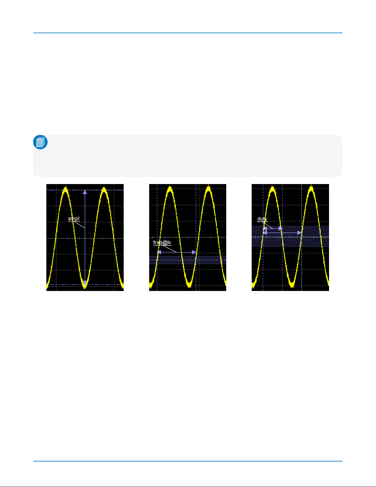
HDO4000/HDO4000A High Definition Oscilloscopes Operator's Manual

Help Markers

Help Markers clarify measurements by displaying lines, labels and hysteresis bands to mark the points
being measured on the trace. For "@Level" parameters, markers make it easier to see where your
waveform intersects the chosen level. If you change the set of parameters displayed, the markers will
change, as well.

You can choose to use Simple markers, which are only the lines, or Detailed markers, which include the
measurement point labels.

You also have the option, by means of the AlwaysOn checkbox, to leave the markers displayed over traces
after you have closed the Measure dialogsor readout table.

Note: Unlike regular cursors, which are white and can be moved, help markers are blue and only
augment the display; they cannot be moved, and they do not reset the measurement points. Some
optional analysis software packages include markers designed specially for that domain of
reference, which are documented in the option manual.

72

Detailed Help Markers.

Find Quality Products Online at: [e-mail]

www.GlobalTestSupply.com

Measure

Gating Measurements

All measurements are calculated on only that portion of the waveform trace that is visible on the grid and
within the measurement gates. Any setting that moves the trace outside the observation window or
makes it appear "clipped" will affect measurements.

The default starting positionsof the measurement gate posts are 0 div and 10 div, which coincide with the
left and right edges of the grid, and the First and Last points. Therefore, the measurement gates initially
enclose the entire visible acquisition. By moving the measurement gates, you can focus the measurement
on the section of the acquisition of greatest interest. For example, if you "gate" six rising edges of a
waveform, calculations are performed only on the six pulses bounded by the gate posts.

The quickest way to set a gate is to drag the gate posts from the far left and right of the grid to the desired
positions. You can refine this position to hundredths of a division by using the Gate Start and Stop fields on
the Measure dialog. All parameters share the same gates, and all measurements will change when you
drag either gate post to reposition the gate.

Touch Default to return the gates to the width of the grid.

Statistics and Histicons

Checking Statistics On on the Measure dialog adds the mean, min, max and sdev of each parameter to the
measured value shown on the Measure table.

Statistics for each parameter are calculated once per acquisition and accumulate until you either Clear
Sweeps or the measurement buffer isfull. The Num row of the Measure table showsthe total number of
measurements included in the Statistics calculation. If the measurement is gated, the statistics are
calculated for only the data points between the gates, just as the parameter value itself will reflect the
limits imposed by the gate.

Mean The weighted mean of the parameter calculated over the number of times shown.

Min The minimum value of the parameter measured over the number of times shown.

Max The maximum value of the parameter measured over the number of times shown.

Sdev The population standard deviation of the parameter calculated over the number of times

shown.

Num For any parameter that computes once on an entire acquisition, Num represents the number

of sweeps over which the statistics are computed.

For any parameter that computes on every event withinan acquisition, such as a full period,
Num represents the number of events per sweep times the number of sweeps computed.
Thus, for a Single acquisitionof five periods, the Num shown for any per period meas­urements will be 5, as five measurements were made and the statistics reflect those five
measurements. After another Single acquisition, Num will be 10, or five measurements
times two sweeps. The statistics now reflect all 10 measurements.

Histicons are miniature histogramsof parameters that may be added to
the Measure table readout. These thumbnailhistograms let you see at a

glance the statistical distribution of each parameter. Check Histicons on the Measure dialog.

73

Find Quality Products Online at: [e-mail]

www.GlobalTestSupply.com

HDO4000/HDO4000A High Definition Oscilloscopes Operator's Manual

List of Standard Measurements

Note: Unless otherwise stated, measurements are calculated according to IEEE standards.
Additional measurements may be available depending on the software options installed.

Amplitude

Difference between the upper and lower levels in two-level (bi-modal) signals. Differs from Peak-to-Peak
(pkpk) in that noise, overshoot, undershoot, and ringing do not affect the measurement. Amplitude is
calculated using the formula for Top-Base. On signals that cannot be identified as bi-modal, such as
triangle or saw-tooth waves, Amplitude returns the same value asMaximum – Minimum. Amplitude may
be calculated once per period, rather than once per acquisition, by selecting "Show one value per period"
on the Amplitude subdialog.

Area

Integral of data. Computes the area of the waveform relative to the zero level. Values greater than zero
contribute positively to the area; values less than zero contribute negatively. If Cyclic ischecked on the
Area subdialog, the area iscalculated over only the full cycles, rather than the entire acquisition.

Base

Lower level in two-level (bi-modal) signals(the higher is Top), or lower of two most probable waveform
states on waveforms that are not bi-modal. Base differs from Minimum in that noise, overshoot,
undershoot and ringing do not affect the measurement. On signals that are not bi-modal (such as triangle
waveforms), Base returns the same value as Minimum. Base may be calculated once per period, rather
than once per acquisition, by selecting "Show one value per period" on the Base subdialog.

Delay

Time from the acquisition trigger to the first 50% level crossing visible in the observation window. On
acquisitions without a Timebase Delay setting, this is usually a negative number.

Dperiod@level

Cycle-to-cycle deviation of the period measurement, measured from rising edges (Pos Slope), falling
edges (Neg Slope), or next crossing (Both Slope) at the specified Level. By default, it measures the
adjacent cycle deviation (cycle-to-cycle jitter) for each cycle in a waveform, but it may be configured to
compare cycles at set intervals or the mean value of groups of cycles by using an N-Cycle Setup.

Dtime@level

Time between transitions on two, different input signals, measured on rising edges (Pos Slope), falling
edges (Neg Slope), or next crossing (Both Slope) at the specified Level. This measurement may yield a
negative result in cases where the Source2 crossing occurs before the Source1 crossing. See Gating

Measurements .

74

Find Quality Products Online at: [e-mail]

www.GlobalTestSupply.com

Measure

Duty Cycle

Percent of period for which data are above or below the 50% level of the signal, using a hysteresisband of
22% of amplitude.

Duty@level

Percent of period for which data are above or below a specified level, measured on rising edges (Pos
Slope) or falling edges (Neg Slope).

Edge@level

Number of edges in waveform that crossthe specified threshold Level, measured on rising edges (Pos
Slope), falling edges (Neg Slope), or next crossing (Both Slope).

Fall 80-20%

Duration of a pulse waveform's falling transition from 80% to 20% of the amplitude, averaged for all falling
transitions between the measurement gates. On signals that do not have two major levels (such as
triangle waveforms), the Top-Base measurement used to calculate the amplitude can default to
maximum and minimum, giving less predictable results.

Fall Time

Duration of a pulse waveform's falling transition from 90% to 10% of the Amplitude, averaged for all falling
transitions between the measurement gates. On signals that do not have two major levels (such as
triangle waveforms), the Top-Base measurement used to calculate the amplitude can default to
maximum and minimum, giving less predictable results.

Frequency

Reciprocal of each Period of a cyclic signal. Period is measured as time between every pair of 50%
crossings on the rising edge, starting with the first rising transition after the left measurement gate.

Freq@level

Reciprocal of each Period of a cyclic signal. Period is measured as the time between every pair of
crossings at the specified level and edge, starting with first matching transition after left measurement
gate.

Maximum

Largest vertical value in a waveform. Unlike Top, does not assume the waveform has two levels.

Mean

Average of vertical values in a waveform. Computed as centroid of distribution for a histogram of the data
values.

Minimum

Smallest vertical value in a waveform. Unlike Base, does not assume the waveform has two levels.

Overshoot-

75

Find Quality Products Online at: [e-mail]

www.GlobalTestSupply.com

HDO4000/HDO4000A High Definition Oscilloscopes Operator's Manual

Amount of overshoot following falling edges, represented as percentage of amplitude. Overshoot- is
calculated using the formula (Base - Minimum)/Amplitude x 100. On signals that do not have two major
levels (such as triangle waveforms), thismeasurement may not give predictable results.

Overshoot+

Amount of overshoot following rising edges, represented asa percentage of amplitude. Overshoot+ is
calculated using the formula (Maximum - Top)/Amplitude x 100. On signals that do not have two major
levels (such as triangle or saw-tooth waveforms), this measurement may not give predictable results.

Peak to Peak

The difference between the maximum and minimum vertical values within the measurement gates.
Unlike Amplitude, does not assume a waveform has two levels.

Period

The time between 50% crossings on the rising edge, starting with the first transition after the left
measurement gate. Period is measured for each adjacent pair, with values averaged to give the final
result.

Period@level

The time between crossingsat a user-specified slope and level, starting with first transition after the left
measurement gate. By default, Period is measured for each adjacent pair, with values averaged to give
the final result, but it can be configured to compare cycles at set intervals by using an N-Period Setup.

Phase

Phase difference between analyzed and reference signals, measured from the 50% level of their rising
edges.

Rise 20-80%

Duration of a pulse waveform's rising transition from 20% to 80% of amplitude, averaged for all rising
transitions between the measurement gates. On signals that do not have two major levels (such as
triangle waves), the Top-Base measurement used to calculate rise can default to maximum and
minimum, giving less predictable results.

Rise Time

Duration of a pulse waveform's rising transition from 10% to 90% of amplitude, averaged for all rising
transitions between the measurement gates. On signals that do not have two major levels (such as
triangle waves), the Top-Base measurement used to calculate rise can default to maximum and
minimum, giving less predictable results.

RMS

Root Mean Square of the vertical values (between the measurement gates), calculated using the formula:

Where: Vi= measured vertical values, and N = number of data points.

76

Find Quality Products Online at: [e-mail]

www.GlobalTestSupply.com

Measure

If Cyclic ischecked on the RMS subdialog, the RMS iscalculated over only full cycles, rather than the
entire acquisition.

Skew

Time of Clock2 edge (Source2) minus the time of previous Clock1 edge (Source1).

Std Dev

Standard deviation of the vertical values between the measurement gates, using the formula:

Where: Vi= measured vertical values, and N = number of data points. Thisis equivalent to the RMS for a
zero-mean waveform. Also referred to as AC RMS.

If Cyclic ischecked on the Std Dev subdialog, the standard deviation is calculated over only full cycles,
rather than the entire acquisition.

Time@level

Time from trigger (t=0) to crossing at a specified slope and level.

Top

Higher vertical value in two-level (bi-modal) signals(the lower is Base), or higher of two most probable
waveform states in waveforms that are not bi-modal. Top differs from Maximum in that noise, overshoot,
undershoot and ringing do not affect the measurement. On signals that are not bi-modal (e.g., triangle
waves), Top returns the same value as Maximum. Top may be calculated once per period, rather than
once per acquisition, by selecting "Show one value per period" on the Top subdialog.

Width

Width of cyclic signal measured at 50% level and positive slope, using a hysteresis of 22% of amplitude.
Widthsof all waveform pulses are averaged for the final result.

WidthN

Width of cyclic signal measured at 50% level and negative slope, using a hysteresis of 22% of amplitude.
Widthsof all waveform pulses are averaged for the final result.

77

Find Quality Products Online at: [e-mail]

www.GlobalTestSupply.com

HDO4000/HDO4000A High Definition Oscilloscopes Operator's Manual

Measure Table

The value row of the Measure table showsthe measurements taken for each parameter on the last
acquisition. You may optionally calculate and display the statistical mean, min, max and sdev of all
parameters. Statistics are calculated once per acquisition and accumulate over multiple acquisitions, up
to the two billion value limit of the measurement buffer.

Close setup dialogs when the Measure table is displayed to maximize the area available for viewing
waveforms. To return to the Measure dialog when closed, touch anywhere in the table.

Symbolsin the statusrow of the Measure table indicate the following:

OK: valid value returned.

Warning: there is a problem with the signal or the setup that prevents measuring. Touch the
parameter cell to see an explanation in the message bar.

No Pulse/Insufficient Data: The software is unable to determine top and base. This may indicate

that there is insufficient difference between the maximum and minimum for the software to
detect a pulse, or there may be an insufficient number of points in the visible top or base of a pulse, such
as when closely examining a step response.

Underflow Condition: The bottom most (negative) sample point of the waveform falls below the

ADC range. Probably, the bottom of the pulses appear to be cut off.

Overflow Condition: The top most (positive) sample point of the waveform is above the ADC

range. Probably, the top of the pulses appear to be cut off.

Simultaneous Underflow and Overflow Condition: Both conditions are present at once.

78

Find Quality Products Online at: [e-mail]

www.GlobalTestSupply.com

Measure

Using Trends

The Trend math function plots a waveform composed of parameter measurements arranged in the order
the measurements were made. The vertical units are the source parameter values, and the horizontal unit
is the measurement number. The Trend containsa single value for each unique measurement, and
therefore may not be time synchronous with the source waveform, where the same measured value may
occur successively over time.

Uses of Trends

Trends are especially useful for visualizing the history of a parameter over an extended period of time or
over multiple acquisitions. Think of Trend as a strip chart recorder for your instrument. Example
applicationsof Trend include:

l Data logging multiple circuit parameters

l Power line monitoring

l Measuring output regulation and ripple

Plotting Trends

Although a Trend plots parameter values, it is created asa Math function on the Function (Fn) dialogs.

1. Select the Trend Operator on the Fn setup dialog.

Tip: On HDO4000 oscilloscopes, you can also touch the Trend button next to the parameter
on the Measure dialog.

2. Choose a computation Mode of All(measurements per acquisition) or Average (one measurement
per acquisition).

3. Enter the number of measured Values to Trend.

79

Find Quality Products Online at: [e-mail]

www.GlobalTestSupply.com

HDO4000/HDO4000A High Definition Oscilloscopes Operator's Manual

80

Find Quality Products Online at: [e-mail]

www.GlobalTestSupply.com

Math

Math

Math function traces (Fn) display the result of applying a mathematical operation to a source trace. The
output of a math function is always another trace, whereas the output of a measurement parameter isa
tabular readout of the measurement.

Math can be applied to any channel (Cn), zoom (Zn), or memory (Mn) trace. It can even be applied to
another math trace, allowing you to chain operations(for example, trace F1 can show the average of C1,
while trace F2 provides the integral of F1).

In addition to the extensive math capabilities that are standard with every instrument, enhanced math
analysis tools customized for various industries and applications are offered through optional software
packages. To learn about math tools available in each optional package, see the product datasheets at

If you have installed software options, the new capabilities are usually accessed through the Analysis
menu, rather than the Math menu, although special math functionswill be available when using the
standard Math dialogs.

Note: If there is a processing error (e.g., overflow) when calculating a math function, a small letter
"i" inside a bubble will appear on the Fn descriptor box to indicate there is more information
regarding the waveform status. See Finding Waveform Status for instructionson finding the error.

Math Function Set Up

Use the Function dialog to set up math function traces. Math functionstake as input one or more channel,
zoom, memory or math traces and output a new math trace (Fn). Any additional settings required for the
operator will appear on a subdialog at the right of the screen.

Single functionsperform one operation on one or two input sources.

Dual functionschain two operations to arrive at a single result. Thissaves you the effort of having to chain
two separate math functions. As with single functions, the number of sources required will vary based on
the operation. You may need only one source for Operator1, but two for Operator2 (the result of the first
operation counts asone source).

Setting Up New Functions

1. From the menu bar choose Math > Math Setup, then open one of the Fn tabs.

Tip: You can select Fn Setup right from the Math menu.

2. Choose a single f(x) or dual g(f(x) operator function.

81

Find Quality Products Online at: [e-mail]

www.GlobalTestSupply.com

HDO4000/HDO4000A High Definition Oscilloscopes Operator's Manual

3. In Operator1, choose the math operation to perform.

4. The choice of operator drives the number of Source fields you will see displayed. Make a selection
in each field, or drag the source channel descriptor box to the field.

A Summary of the function you are building appears on the dialog. Refer to this to be sure your
sources are in the proper order to yield the function you want (e.g., C1-C2 vs. C2-C1).

5. If the operator you've selected has any other configurable settings, you'll see a subdialog of the
same name as the operator. Touch the tab to open the dialog and make any further settings. These
are explained on the dialog.

6. If you're creating a dual function, repeat the procedure for the second operator.

Adjusting Memory or Math Traces

Unlike channel traces, the scale of memory (Mn) or math function (Fn) traces can be adjusted directly
without having to create a separate zoom trace. The same set of zoom factor controlsused for zoom
traces appear on the Zoom subdialog, but in this context they only rescale the active math or memory
trace rather than create a new zoom. This applies to any trace that iscreated asa math function (Fn)
trace, including traces generated through analysisoptions and graphs.

You can, if you wish, create a separate zoom trace from a memory or function trace the same as you
would normally create a zoom (draw a selection box, etc.). In this case, you choose one of the zoom
locations (Zn) in which to draw the trace, but the source trace remains at the original scale.

82

Find Quality Products Online at: [e-mail]

www.GlobalTestSupply.com

Math

List of Standard Math Operators

Note: The installation of software options on the oscilloscope may add math operators to thislist.

Absolute

Calculates distance away from zero for every point in the waveform. For values greater than zero, this is
the same as the value. For values less than zero, the magnitude without regard to its sign is used.

Average

Calculates either a summed or continuous average of a selected number of sweeps. See Averaging

Waveforms. The maximum number of sweeps is determined by the oscilloscope model and memory.

Derivative

Calculates the derivative of adjacent samples using the formula:

(next sample value – current sample value) / (horizontal sample interval)

Difference

For every point in the waveform, subtracts the value of Source2 from the value of Source1. Source1 and
Source2 must have the same horizontal and vertical units and scale.

Envelope

Calculates highest and lowest vertical values of a waveform at each horizontal value for a specified
number of sweeps.

ERes

Applies a noise reduction and smoothing filter by adding a specified number of bits. See Enhanced

Resolution.

FFT

Computes a frequency spectrum with optional Rectangular, Von Hann, Flat Topp, Hamming, Blackman­Harris, and Hanning windows. Calculates up to 128 Mpts. Also allows FFT Averaging through use of a
second math operator. See FFT.

Floor

Calculates the lowest vertical values of a waveform at each horizontal value for a specified number of
sweeps.

Integral

Calculates the linearly rescaled integral (with multiplier and adder) of a waveform input starting from the
left edge of the screen using the formula:

(current sample value + next sample value) * (horizontal sample interval)

83

Find Quality Products Online at: [e-mail]

www.GlobalTestSupply.com

HDO4000/HDO4000A High Definition Oscilloscopes Operator's Manual

Each calculated area issummed with the previous sum of areas. The multiplier and adder are applied
before the integration function.

Invert

For every point in the waveform, the inverse of that point is calculated.

Product

For every point in the waveform, the value of Source1 is multiplied by the value of Source 2. Source1 and
Source2 must have the same horizontal units and scale.

Ratio

For every point in the waveform, divides the value of Source1 by the value of Source2. Source1 and
Source2 must have the same horizontal units and scale.

Reciprocal

For every point in the waveform, calculates the inverse using the formula: 1 / (sample value).

Rescale

For every point in the waveform, multiplies the sample value by the specified Multiplier, then addsthe
specified Additive Constant value. See Rescaling and Assigning Units.

Roof

Calculates the highest vertical value at each sample point for a specified number of sweeps.

Square

For every point in the waveform, calculates the square of the sample value.

Square Root

For every point in the waveform, calculates the square root of the sample value.

Sum

For every point in the waveform, addsthe value of Source1 to the value of Source 2. Source1 and Source2
must have the same horizontal and vertical units and scale.

Trend

Produces a waveform composed of a series of measurement parameter values in the order the
measurements were taken. The vertical units are those of the source parameter; the horizontal unit is
measurement number. The trend contains a single value for each unique measurement.

Zoom

Produces a magnified trace of a selected portion of the input waveform. See Zooming Traces.

84

Find Quality Products Online at: [e-mail]

www.GlobalTestSupply.com

Math

Average Function

The summed or continuous average of all data samples from multiple acquisitions can be displayed as a
new waveform trace using the Average function.

Setting Up Averaging

To apply Continuous or Summed Averaging asa Math function:

1. Follow the usual steps to set up a math fuction, selecting Average from the Basic Math submenu.

2. On the Average subdialog, choose Summed or Continuous.

3. Touch Sweeps and provide a value.

Tip: To quickly set up Continuous Averaging (only), access the channel setup dialog (Cn) and enter
the number of sweeps to average in Averaging.

Summed Averaging

Summed Averaging is the repeated addition, with equal weight, of successive source waveform records. If
a stable trigger is available, the resulting average has a random noise component lower than that of a
single-shot record. Whenever the maximum number of sweeps isreached, the averaging process stops. In
Summed averaging, you specify the number of acquisitionsto be averaged. The averaged data is updated
at regular intervals.

An even larger number of records can be accumulated simply by changing the number in the dialog.
However, the other parameters must be left unchanged or a new averaging calculation will be started. You
can pause the averaging by changing the trigger mode from Normal/Autoto Stop. The instrument
resumes averaging when you change the trigger mode back to Normal/Auto.

You can reset the accumulated average by pushing the Clear Sweeps button or by changing an acquisition
parameter such as input gain, offset, coupling, trigger condition, timebase, or bandwidth limit. The number
of current averaged waveforms of the function, or itszoom, is shown in the acquisition status dialog. When
summed averaging is performed, the display is updated at a reduced rate to increase the averaging speed
(points and events per second).

Continuous Averaging

Continuous Averaging, the default setting, is the repeated addition, with unequal weight, of successive
source waveforms. It is particularly useful for reducing noise on signalsthat drift very slowly in time or
amplitude. The most recently acquired waveform has more weight than all the previously acquired ones:
the continuousaverage isdominated by the statistical fluctuations of the most recently acquired
waveform. The weight of ‘old'waveforms in the continuous average tends to zero (following an
exponential rule) at a rate that decreases as the weight increases.

You determine the importance of new data vs. old data by assigning a weighting factor. The formula for
continuousaveraging is:

new average = (new data + weight * old average)/(weight + 1)

85

Find Quality Products Online at: [e-mail]

www.GlobalTestSupply.com

HDO4000/HDO4000A High Definition Oscilloscopes Operator's Manual

By setting a Sweeps value, you establish a fixed weight that is assigned to the old average once the
number of sweeps isreached. For example, for a sweeps (weight) value of 4:

Sweep New Average =

1 (no old average yet) (new data +0 * old average)/(0 + 1) = new data only

2 (new data + 1*old average)/(1 + 1) = 1/2 new data +1/2 old average

3 (new data + 2 * old average)/(2 + 1) = 1/3 new data + 2/3 old average

4 (new data + 3 * old average)/(3 + 1) = 1/4 new data + 3/4 old average

5 (new data + 4 * old average)/(4 + 1) = 1/5 new data + 4/5 old average

6 (new data + 4 * old average)/(4 + 1) = 1/5 new data + 4/5 old average

7 (new data + 4 * old average)/(4 + 1) = 1/5 new data + 4/5 old average

Note: The number of sweeps used to compute the average is displayed at the bottom of the trace
descriptor box.

86

Find Quality Products Online at: [e-mail]

www.GlobalTestSupply.com

ERes Function

ERes (Enhanced Resolution) filtering increases vertical resolution, allowing you to distinguish closely
spaced voltage levels. The instrument's ERes function is similar to smoothing the signal with a simple,
moving-average filter, but is more efficient concerning bandwidth and pass-band filtering. Use ERes:

l On single acquisitionsor where the data isslowly repetitive (and you cannot use averaging).

l To reduce noise on noticeably noisy signals when you do not need to perform noise measurements.

l Asa low-pass filter. The ERes filter rejects high-frequency components from the signal. The higher

the bit enhancement, the lower the resulting bandwidth.

l When performing high-precision voltage measurements (e.g., zooming with high vertical gain).

Setting Up ERes

To apply ERes as a Math function:

1. Follow the usual steps to set up a math function, selecting Eres from the Filter submenu.

2. Touch the Trace On checkbox.

Math

3. On the Eres subdialog, select the number of bits of improvement from the pop-up menu.

How ERes Is Applied

The instrument's ERes feature improves vertical resolution by a fixed amount for each filter. This real
increase in resolution occurs whether or not the signal is noisy, or whether it is single-shot or repetitive.
The signal-to-noise ratio (SNR) improvement depends on the form of the noise in the original signal. ERes
filtering decreases the bandwidth of the signal, filtering out some of the noise.

The instrument's constant phase finite impulse response (FIR) filters provide fast computation, excellent
step response in 0.5 bit steps, and minimum bandwidth reduction for resolution improvements of between

0.5 and 3 bits. Each step corresponds to a bandwidth reduction factor of two, allowing easy control of the
bandwidth resolution trade-off.

Resolution Increase

0.5 0.5 2

1.0 0.241 5

1.5 0.121 10

2.0 0.058 24

2.5 0.029 51

3.0 0.016 117

-3 dB Bandwidth (x Nyquist) Filter Length (Samples)

With low-passfilters, the actual SNR increase obtained in any particular situation depends on the power
spectral density of the noise on the signal.

87

Find Quality Products Online at: [e-mail]

www.GlobalTestSupply.com

HDO4000/HDO4000A High Definition Oscilloscopes Operator's Manual

The improvement in SNR correspondsto the improvement in resolution if the noise in the signal is white
(evenly distributed across the frequency spectrum). If the noise power is biased towardshigh frequencies,
the SNR improvement willbe better than the resolution improvement.

The opposite may be true if the noise is mostly at lower frequencies. SNR improvement due to the
removal of coherent noise signals—feed-through of clock signals, for example—is determined by the fall of
the dominant frequency components of the signal in the passband. This is easily ascertained using
spectral analysis. The filters have a precisely constant zero-phase response. This has two benefits. First,
the filters do not distort the relative position of different events in the waveform, even if the events'
frequency content is different. Second, because the waveforms are stored, the delay normally associated
with filtering (between the input and output waveforms) can be exactly compensated during the
computation of the filtered waveform.

The filters have been given exact unity gain at low frequency. ERes should therefore not cause overflow if
the source data is not overflowed. If part of the source trace were to overflow, filtering would be allowed,
but the results in the vicinity of the overflowed data—the filter impulse response length—would be
incorrect. This is because in some circumstances an overflow may be a spike of only one or two samples,
and the energy in this spike may not be enough to significantly affect the results. It would then be
undesirable to disallow the whole trace.

Note: While ERes improves the resolution of a trace, it cannot improve the accuracy or linearity of
the original quantization. The pass-band causes signal attenuation for signalsnear the cut-off
frequency. The highest frequencies passed may be slightly attenuated. Perform the filtering on
finite record lengths. Data is lost at the start and end of the waveform and the trace ends up
slightly shorter after filtering. The number of samples lost is exactly equal to the length of the
impulse response of the filter used: between 2 and 117 samples. Normally this loss(just 0.2 % of a
50,000 point trace) is not noticed. However, you might filter a record so short that no data is
output. In that case, however, the instrument would not allow you to use the ERes feature.

88

Find Quality Products Online at: [e-mail]

www.GlobalTestSupply.com

Math

FFT Function

For a large classof signals, you can gain greater insight by looking at spectral representation rather than
time description. Signalsencountered in the frequency response of amplifiers, oscillator phase noise and
those in mechanical vibration analysis, for example, are easier to observe in the frequency domain.

If sampling is done at a rate fast enough to faithfully approximate the original waveform (usually five times
the highest frequency component in the signal), the resulting discrete data series will uniquely describe
the analog signal. This is of particular value when dealing with transient signals, which conventional swept
spectrum analyzers cannot handle.

While FFT has become a popular analysis tool, some care must be taken with it. In most instances,
incorrect positioning of the signal within the display grid will significantly alter the spectrum, producing
effects such as leakage and aliasing that distort the spectrum.

An effective way to reduce these effects is to maximize the acquisition record length. Record length
directly conditions the effective sampling rate and therefore determines the frequency resolution and
span at which spectral analysis can be carried out.

Setting Up FFT

1. Follow the usual steps to set up a math function, selecting FFT from the Frequency Analysis
submenu.

2. Open the FFT subdialog.

3. Choose an Output type.

4. If your Output Type isPower Spectrum, also enter Line Impedence. By default, the FFT function
assumes a termination of 50 Ohms. If an external terminator is being used, this setting can be
changed to properly calculate the FFT based on the new termination value.

5. Optionally, choose a weighting Window (see below).

6. Check the SuppressDC box to make the DC bin go to zero. Otherwise, leave it unchecked.

Choosing a Window

If you think of an FFT as synthesizing a bank of parallel band-passfilters, weighting functions control the
filter response shape and affect noise bandwidth as well as side lobe levels. Ideally, the main lobe should
be as narrow and flat as possible to effectively discriminate all spectral components, while all side lobes
should be infinitely attenuated. The window type defines the bandwidth and shape of the equivalent filter
to be used in the FFT processing.

The choice of a spectral window is dictated by the signal's characteristics. Rectangular windows provide
the highest frequency resolution and are useful for estimating the type of harmonics present in the signal.
Because the rectangular window decays as a (SinX)/X function in the spectral domain, slight attenuation
will be induced. Functions with less attenuation (Flat Top and Blackman-Harris) provide maximum
amplitude at the expense of frequency resolution, whereas Hamming and Von Hann are good for general
purpose use with continuous waveforms.

89

Find Quality Products Online at: [e-mail]

www.GlobalTestSupply.com

HDO4000/HDO4000A High Definition Oscilloscopes Operator's Manual

Window Type Applications and Limitations

Rectangular Normally used when the signal is transient (completely contained in the time-domain window)

or known to have a fundamental frequency component that is an integer multiple of the fun­damental frequency of the window. Signals other than these types will show varying amounts of
spectral leakage and scallop loss, which can be corrected by selecting another type of window.

Hanning (Von Hann)
& Hamming

Flat Top Provides excellent amplitude accuracy with moderate reduction of leakage, but with reduced

Blackman-Harris Reduces leakage to a minimum, but with reduced frequency resolution.

Reduces leakage and improves amplitude accuracy. However, frequency resolution is also
reduced.

frequency resolution.

FFT Window Filter Parameters

Window Type

Rectangular

Von Hann

Hamming

Flat Top

Blackman-Harris

Highest Side Lobe
(dB)

-13 3.92 1.0 0.0

-32 1.42 1.5 -6.02

-43 1.78 1.37 -5.35

-44 0.01 3.43 -11.05

-67 1.13 1.71 -7.53

Scallop Loss (dB) ENBW (bins) Coherent Gain (dB)

90

Find Quality Products Online at: [e-mail]

www.GlobalTestSupply.com

Math

Rescale Function

The Rescale function allowsyou to create a new function trace that rescales another trace by applying a
multiplication factor (a) and additive constant (b). You can also use it as a way to view the function source
in a different unit of measure.

Setting Up Rescaling

1. Follow the usual steps to set up a math function, selecting Rescale from the Functions submenu.

2. Touch the Rescale subdialog tab.

3. To modify the scale of output:

l Check the First multiply by: box and enter the number of units equal to 1 V (a, the multiplication

factor).

l Touch then add: and enter b, the additive constant.

4. To change the output unit of measure from that of the source waveform:

l Check Override units.

l In Output enter the code for the new unit of measure.

You can combine units following these rules:

l For the quotient of two units, use the character "/"

l For the product of two units, use the character "."

l For exponents, append the digit to the unit without a space (e.g., "S2" for secondssquared)

Note: Some complex units are automatically converted to simple units. For example, V.A

becomes W).

Units of Measure

Units are automatically rescaled up or down within the list of standard, SI prefixes based on the relative
size of the signal. For example a 1000 V reading is shown as 1 kV, while .1 V is shown as 100 mV. When
the multiplication factor is 1 V = 1 Pascal, a 10 millivolt (mV) reading is displayed as 10 mPa rather than
.001 Pa or 100e-3 Pa.

Following are the supported SI units of measure and the mnemonics used to represent them on the
Rescale dialog.

Note: These same mnemonics can be used in remote control programs and customization
scripts. Specify only the base unit in code, do not add prefixes.

91

Find Quality Products Online at: [e-mail]

www.GlobalTestSupply.com

HDO4000/HDO4000A High Definition Oscilloscopes Operator's Manual

Note: Time and dimensionlessunits are available only for certain measurements and for use in
code where relevant.

Category Unit Mnemonic

Mass gram G

slug SLUG

Volume liter L

cubic meter M3

cubic inch IN3

cubic foot FT3

cubic yard YARD3

Angle radian RAD

arcdegree DEG

arcminute MNT

arcsecond SEC

cycle CYCLE

revolution REV

turn TURN

Force/Weight Newton N

grain GR

ounce OZ

pound LB

Velocity meters/second M/S

inches/second IN/S

feet/second FT/S

yards/second YARD/S

miles/second MILE/S

Acceleration meters/second

inches/second

feet/second

standard gravity GN

2

2

2

M/S2

IN/S2

FT/S2

92

Find Quality Products Online at: [e-mail]

www.GlobalTestSupply.com

Category Unit Mnemonic

Pressure Pascal PAL

bar BAR

atmosphere, technical AT

atmosphere, standard ATM

Torr TORR

pounds/square inch PSI

Temperature degrees Kelvin K

degrees Celsius CEL

degrees Fahrenheit FAR

Energy Joule J

British Thermal Unit BTU

calorie CAL

Rotating Machine radians/second RADPS

frequency (Hertz) HZ

Math

revolutions/second RPS

revolutions/minute RPM

torque N•m NM

torque in•oz INOZ

torque in•lb INLB

torque ft•lb FTLB

power, mechanical (Watt) W

horsepower HP

Magnetic Weber WB

Tesla T

inductance (Henry) H

magnetic field strength A/M

permeability HENRYPM

93

Find Quality Products Online at: [e-mail]

www.GlobalTestSupply.com

HDO4000/HDO4000A High Definition Oscilloscopes Operator's Manual

Category Unit Mnemonic

Electrical Ampere A

Volt V

Watt W

power, apparent VA

power, reactive VAR

power factor PF

capacitance (Farad) F

Coulomb C

Ohm OHM

Siemen SIE

electrical field strength V/M

electrical displacement field CPM2

permittivity FARADPM

conductivity SIEPM

Time second S

minute MIN

hour HOUR

day DAY

week WEEK

94

Find Quality Products Online at: [e-mail]

www.GlobalTestSupply.com