Teledyne JTA2 User Manual

JTA2

Jitter & Timing Analysis

Operator’s Guide

December 2003

LeCroy Corporation

700 Chestnut Ridge Road
Chestnut Ridge, NY 10977–6499
Tel: [phone], Fax: [phone]

Internet: www.lecroy.com

© 2003 by LeCroy Corporation. All rights reserved.

LeCroy, ActiveDSO, ProBus, SMART Trigger, JitterTrack, WavePro, WaveMaster, and
Waverunner are registered trademarks of LeCroy Corporation. Information in this publication
supersedes all earlier versions. Specifications subject to change without notice.

JTA2-OM-E Rev A
902145

ACCESSING JTA2...............................................................................................3

TIMING FUNCTIONS............................................................................................3

TIMING PARAMETERS........................................................................................4

Statistical Tools.................................................................................................................................4

HOW JITTERTRACK WORKS.............................................................................5

Using “Clock” or “Data” ....................................................................................................................5

WHEN TO USE JITTERTRACK...........................................................................7

JitterTrack or Trend? ................................................................................................................7

CLOCK OR DATA?..............................................................................................9

SETTING UP JITTER MEASUREMENTS..........................................................11

Jitter Math Setup............................................................................................................................11

JitterTrack...............................................................................................................................12

Jitter Parameters Setup .................................................................................................................12

WHEN TO USE PERSISTENCE HISTOGRAMS................................................14

SETTING UP PERSISTENCE HISTOGRAMS ...................................................15

Selecting the Math Function...........................................................................................................15

Setting Up the Histogram...............................................................................................................16

Selecting the Cut.....................................................................................................................16

HOW TO TRACE PERSISTENCE...................................................................... 17

An Innovative Visual and Processing Tool.....................................................................................17

To Set Up Trace Persistence..........................................................................................................18

CHOOSING A TIMING PARAMETER................................................................20

HOW TO USE THE TREND TOOL.....................................................................21

The Basic Idea ...............................................................................................................................21

To Set Up and Configure Trend .....................................................................................................22

Parameter Setup.....................................................................................................................22

Math Setup..............................................................................................................................24

HISTOGRAM AND TREND CALCULATION .....................................................25

Acquisition Sequence.....................................................................................................................25

Parameter Buffer............................................................................................................................25

Parameter Events Capture.............................................................................................................26

Zoom Traces and Segmented Waveforms.....................................................................................26

Histogram Peaks.....................................................................................................................26

Example..................................................................................................................................27

Binning and Measurement Accuracy......................................................................................27

JTA2-OM-E Rev A ISSUED: December 2003 1

JTA2 Option

BLANK PAGE

2 ISSUED: December 2003 JTA2-OM-E Rev A

ACCESSING JTA2

To access JTA2's special features, you must first purchase and install the option. Once installed,
JTA2's math and parameter selections will app ear in the Math and Measure menus.

TIMING FUNCTIONS

JitterTrack, PersistenceHistogram and PersistenceTrace are timing functions in LeCroy’s JitterPro
and JTA jitter and timing analysis packages. The JitterTrack feature is key to identifying the
source of excessive jitter or non-normal jitter characteristics. A timel ine of signal jitter that is
synchronous with the signal under test allows you to view patterns that would remain invisible
using other systems, zoom to areas containing maximum jitter, and troubleshoot the problem.
PersistenceHistogram is the ideal quantitative "companion" to persisten ce display. It histograms a
horizontal or vertical slice of the persistence waveform. Utilizing average, si gma, and range
settings, PersistenceTrace comp utes a vector trace from a bit map to give insight into edge
details down to a few picoseconds.

• JitterTrack graphically plots as a function of time the amplitude of the waveform
attributes Cycle-to-Cycle variation, Duty Cycle, Interval Error, Period, Width, and
Frequency. Interval Error, for example, calculates the timing error of a signal compared
with an ideal, expected interval defined by a user-specified reference frequency, the most
common estimator of jitter. "The sho rt-te rm variations of a digital signal’s significant
instants, from their ideal positions in time," are plotted. This is the perfect tool for
characterizing clocks in synchronized telecom networks such as SONET and SDH. A
special data function, available for most of these attributes, enables work on random data
streams.

• Persistence Histogram analyzes a vertical or horizontal slice of a persistence map of
multiple waveforms. The resultant bar chart shows a numerical measurement of the
timing variations of a signal, which are observed qualitatively in the persistence display of
the signal. A typical application is characterizing the jitter in a communications signal eye
diagram.

• Persistence Trace is a method for displaying the data acquired from multiple sweeps of
a waveform. A vector trace is computed, based on the bit map of the underlying multiple
signal acquisitions. Detail is then represented in a choice of three graphic forms, each
representing a different characteristic of the waveform. Insight into edge details is given
down to a few picoseconds — valuable in applications such as the examination of fast
signal transitions.

JTA2-OM-E Rev A ISSUED: December 2003 3

JTA2 Option

TIMING PARAMETERS

Timing parameters can also be used to measure cycle-to-cycle jitter , the width of positive and
negative pulses, the duty cycle of either polarity, and an infinite number of cycles on long records.
Pulses or cycles can be counted using one of these parameters.

As interpolation filtering is applied to signal edges in the vicinity of measurement points, timing
parameters operate on acquired waveform levels that may be selected in either volts or
percentage of signal amplitude. Each parameter calculation is performed over all cycles or edges
present in the input signal, without limitations.

Statistical Tools

The information obtained from applying timing parame ters can then be analyzed using the
statistical tools, histograms and trends:

• Histograms characterize and present as a bar chart the statistical distribution of a timing
parameter’s set of values. In addition, there are 18 statistical histogram parameters,
which operate directly on the histogram.

• Trends represent the evolution of timing parameters in line graphs whose vertical axes
are the value of the parameter, and horizontal axes the order in which the values were
acquired.

4 ISSUED: December 2003 JTA2-OM-E Rev A

HOW JITTERTRACK WORKS

Using “Clock” or “Data”

Use this function to plot as a bar chart the evolution over time of this and five other waveform
attributes in simple steps.

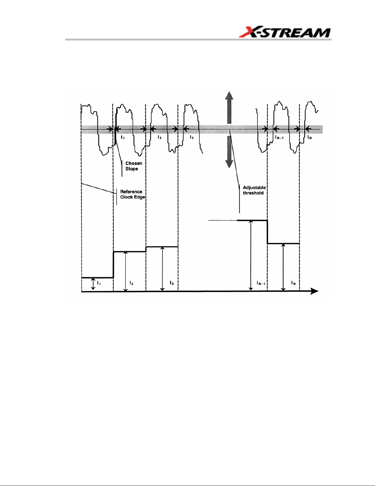
How JitterTrack’s Interval Error works when “Clock” Mode is selected

JTA2-OM-E Rev A ISSUED: December 2003 5

JTA2 Option

When “Data” Mode is selected.

1. Set the desired reference clock frequency for an ideal position against which the signal is
to be compared, or use “Find Frequency.”

2. Specify the level at which the jitter measurement is to be made, as well as the rising or
falling edge on which the measurement is to start.

3. Timing errors are graphically revealed.

6 ISSUED: December 2003 JTA2-OM-E Rev A

WHEN TO USE JITTERTRACK

The JitterTrack Function chart s the evolu t ion in time of these waveform attributes :

• Cycle-to-Cycle deviation

• Duty Cycle

• Interval Error

• Period

• Pulse Width

• Frequency

Each is time-correlated to its source trace and contains the same number of points as the
waveform.

JitterTrack or Trend?

Whether it is more appropriate to use JitterTrack or the statistical tool, Trend will largely depend
on the application, as well as the other factors set out in the tables below. While JitterTrack
sample points are evenly spaced in time, those of Trend are not. Trend plots any parameter
available in the instrument against its event count, as in a scatter or an XY diagram.

Characteristic Trend JitterTrack
Representation parameter Value vs. Events attribute value vs. time
Attributes or

Parameters Supported

Behavior cumulative over several

JTA2-OM-E Rev A ISSUED: December 2003 7

all parameters Cycle-Cycle

Period
Duty Cycle
Width
Interval Error
Frequency

non-cumulative
acquisitions
up to 1 million events

(resets after every acquisiti on)

unlimited number of events

JTA2 Option

When you need to Use…

monitor the evolution of a waveform parameter
or attribute over several acquisitions...

time-correlate an event and a parameter value...
monitor an evolution in the frequency domain... JitterTrack - Trend points are not evenly

monitor JT A parameters...

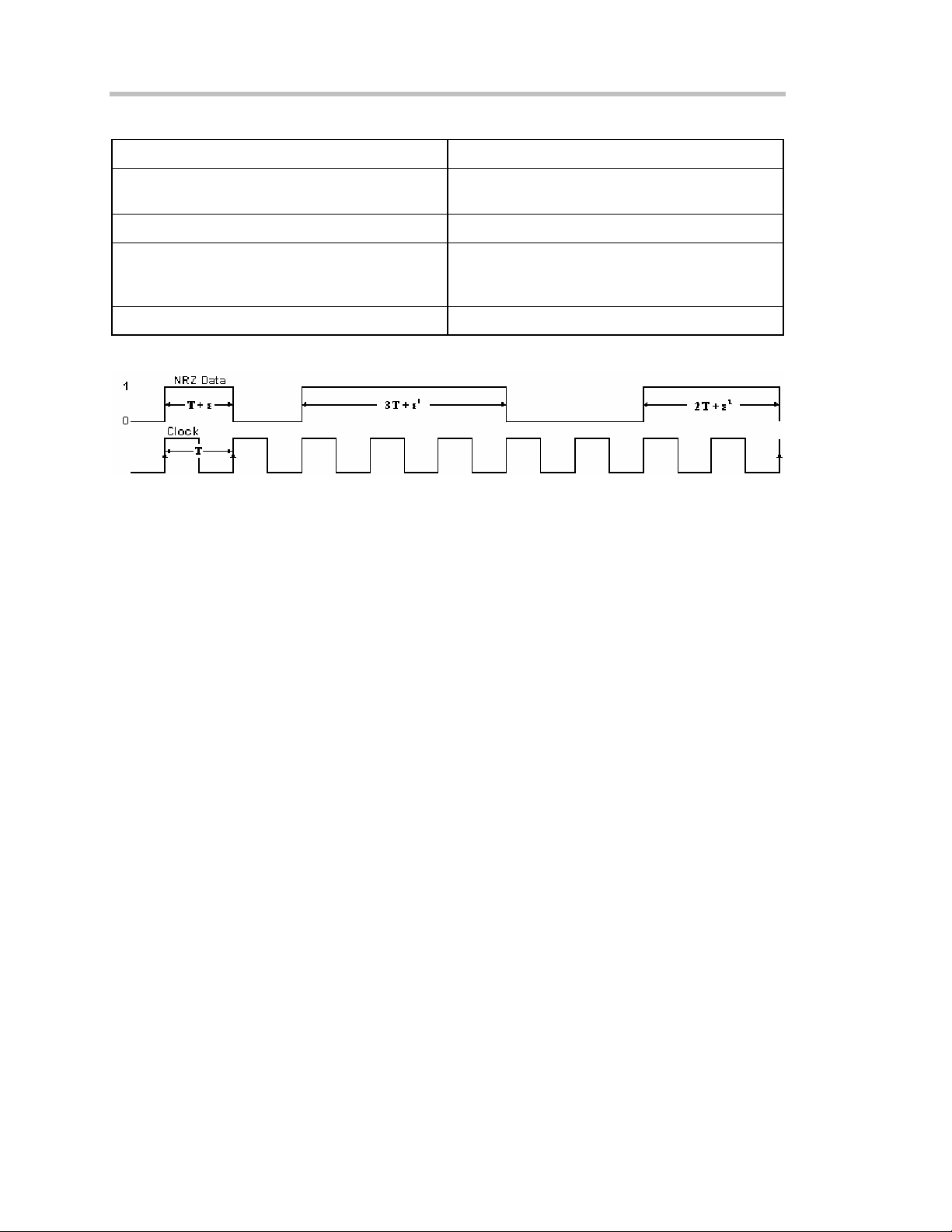
Random NRZ (Non-Return to Zero) data stream and its corresponding clock signal.

Trend - Jitter works only on one acquisition at a

time
JitterTrack

spaced in time and therefore cannot be used
for FFT (Fast Fourier Transform).

Trend

8 ISSUED: December 2003 JTA2-OM-E Rev A

CLOCK OR DATA?

For most waveform attributes, JitterTrack offers the choice of Clock or Data modes for measuring
clock signals or data streams. "Data" should be used (where available) when the pulse widths,
intervals, periods or other significant instants being measured are randomly distributed and
contain multiples of the clock period.

On the one hand, apart from jitter, clock signals ought to be regular. On the other hand, data
streams by their very nature have irregular pulse widths.

A clock signal is normally required to characterize jitter . But such a signal will not be available if
the waveform being measured is a data stream, whose very randomness hides the clock signal.
To overcome this, JitterTrack provides both Clock and Data modes. Selecting Data from the
VClock dialog gives the superior timing resolution through normalization (see tab le) required for
correctly measuring jitter in data signals.

The diagram on the previous page shows a data stream in relation to its clock signal. It illustrates
how data pulses contain, within themselves, multiples of their clock-signal pulse widths. Analyzing
the positive pulses in the data stream, we observe a great variance between each sample in, for
instance, the range Τ to 3Τ . In fact, it is the small variations (the jitter) that are important. And
they could be normalized if clock frequency, and clock frequency over pulse width, were known.
This normalization, provided by JitterTrack, reduces pulse variations and increases timing
resolution so that errors (ε ) can be clearly observed. It does this by reducing the jitter range,
dividing each measurement equal to n × Τ by n.

JTA2-OM-E Rev A ISSUED: December 2003 9

JTA2 Option

Comparing a Random Data Stream Analyzed Using Clock and Data Modes.

Modes CLOCK DATA

Jitter Range
Resolution

3Τ + ε ε << 3Τ

coarse fine

10 ISSUED: December 2003 JTA2-OM-E Rev A

SETTING UP JITTER MEASUREMENTS

Jitter Math Setup

1. Touch Math in the menu bar, then Math Setup... in the drop-down menu.

2. In the "Math" dialog, touch an unused Fx button to simply make a selection from the

Select Math Operator menu. Or , touch an Fx tab

for more setup

options.

Note: By default, unused Fx positions are designated as zooms of C1. However, the traces are disabled, as indicated by
an unchecked On box alongside the Fx button:

3. Touch the Jitter Functions button in the Select Math Opera tor menu for a list of
persistence functions.

JTA2-OM-E Rev A ISSUED: December 2003 11

JTA2 Option

4. Touch a persistence function. The Select Math Operator menu closes, and the trace is
automatically enabled.

JitterTrack

If you want to enable JitterTrack in addition to (or instead of) a persistence function trace, touch
the Jitter button in the Select Math Operator menu, then the Track button. The Select Math

Operator menu closes, and the JitterTra ck is automatically enabled.

Jitter Parameters Setup

1. Touch Measure in the menu bar, then Measure Setup... in the drop-down menu.

2. Touch the My Measure button

3. In the "Measure" dialog, touch an unused Px button to simply select a jitter parameter
from the Select Measurement menu. Or, touch a Px tab for more setup options.

4. Touch the Jitter button in the Select Measurement menu; a list of persisten ce functions

12 ISSUED: December 2003 JTA2-OM-E Rev A

.

appears.

5. Touch a parameter. The setup dialog for the Px position you selected opens
automatically. A mini-dialog also opens to the right of the main dialog, giving you more
setup options for the selected parameter.

JTA2-OM-E Rev A ISSUED: December 2003 13

JTA2 Option

WHEN TO USE PERSISTENCE HISTOGRAMS

The Persistence Histogram function builds a histogram from a persistence map to reveal the
features that are only visible when several acquisitions have been superimposed on one anot her.
In contrast to this, the histogram as statistical tool simply graphs waveform parameters such as
amplitude, frequency, or pulse width on an acquisition or series of acquisitions.

Both Histogram and Persistence Histogram bar charts are divided into intervals, or bins. While
each bin in the histogram bar chart contains a class of similar pa rameter values, the Persistence
Histogram analyzes both vertical and horizontal "slices" of the persistence map. Vertically, each
bin contains a class of similar amplitude levels; horizontally, each bin contains a class of similar
time values.

For a Histogram of Use
a crossover point in time or in amplitude on an

eye diagram
cumulative jitter on an eye diagram Persistence Histogram (Horiz. Slice)
signal-to-noise ratio on an eye diagram Persistence Histogram (Vert. Slice)
the different interval widths present in a long

data stream
cumulative jitter on a long record of a clock

signal
cycle-to-cycle jitter

Persistence Histogram (Vert. and Horiz. Slices)

Histogram (of Timing Parameter p@lv)

Histogram (of Timing Parameter tie@lv)

Histogram (of

∆

p@lv)

14 ISSUED: December 2003 JTA2-OM-E Rev A

SETTING UP PERSISTENCE HISTOGRAMS

Selecting the Math Function

1. Touch Math in the menu bar, then Math Setup... in the drop-down menu.

2. In the "Math" dialog, touch an unused Fx button to simply make a selection from the

Select Math Operator menu. Or , touch an Fx tab

for more setup

options.

Note: By default, unused Fx positions are designated as zooms of C1. However, the traces are disabled, as indicated by
an unchecked On box alongside the Fx button:

3. Touch the Jitter Functions button in the Select Math Opera tor menu,

then touch the Phistogram button

. A setup mini-dialog opens to the right of the

main dialog.

JTA2-OM-E Rev A ISSUED: December 2003 15

JTA2 Option

Setting Up the Histogram

The mini-dialog contains setup fields for your histogram.

Selecting the Cut

Touch inside the Cut Direction field
Horizontal. If you choose to cut a vertical slice, the units of the center and width of the slice are

given in nanoseconds. If you choose a horizontal cut , the units of the center and width of the slice
are given in millivolts.

16 ISSUED: December 2003 JTA2-OM-E Rev A

and select either Vertical or

HOW TO TRACE PERSISTENCE

A persistence waveform created by turning on persistence is show here. From this waveform, you
can create three types of shapes on which waveform processing can be performed.

From left to right are shown Average, Range, and Sigma

An Innovative Visual and Processing Tool

With this timing function, not only can waveform noise and jitter be displayed but further
processing can also be done.

Persistence T race gen erates special graphic representations of the persistence waveform on
which further processing, such as the application of parameters an d even Pass/Fail testing, can
be performed.

JTA2-OM-E Rev A ISSUED: December 2003 17

JTA2 Option

Displaying data acquired from multiple sweeps of the waveform, Persistence Trace computes a
vector trace based on the bit map of the underlying signal acquisitions. Detail is then shown in a
choice of three shapes: average, range, and sigma. These are created without destroying the
underlying data, allowing the display of analytical results from raw data.

Typical appli cations of Persistence Trace are given in this table:

If you want to Use
see edge detail in a fast signal average
eliminate noise on a persistence trace average
assess typical noise on a persistence trace sigma
assess worst case noise on a persistence trace

range

and use it to create a tolerance mask

To Set Up Trace Persistence

1. Touch Math in the menu bar, then Math Setup... in the drop-d own menu.

2. In the "Math" dialog, touch an unused Fx button to simply make a selection from the

Select Math Operator menu. Or , touch an Fx tab

for more setup

options.

Note: By default, unused Fx positions are designated as zooms of C1. However, the traces are disabled, as indicated by
an unchecked On box alongside the Fx button:

3. Touch the Jitter Functions button in the Select Math Opera tor menu, then touch one of
the Persistence Trace buttons:

Ptrace Mean

Ptrace Range

Ptrace Sigma

18 ISSUED: December 2003 JTA2-OM-E Rev A

A setup mini-dialog o pens to the right of the main dialog, offering the following additional setup
options:

Function Options How It Works

Ptrace Mean Clear Sweeps For each vertical time slice on

the persistence map, Ptrace
Mean calculates and plots a
trace corresponding to the
map’s mean value. Single-shot
signals sampled at or above 2
GS/s and accumulated in the
persistence map can be traced
at a resolution of 10 ps (100
GS/s equivalent sampling). The
persistence trace average can
be further analyzed using the
instrument’s standard
parameters, such as rise time.

Ptrace Range Clear Sweeps, % population

range. A percentage of the
population of the persistence
map can be chosen from which
the envelope will be formed,
enabling exclusion of infrequent
events (artifacts).

Ptrace Sigma Clear Sweeps, Scale to

standard deviations. This allows
you to select a sigma from 0.5
to 10.0, which expands those
parts of the sigma envelope
representing waveform regions
with the most jitter. This is
useful for making a tolerance
mask.

For each vertical time slice on
the persistence map, Ptrace
Range calculates and plots an
envelope corresponding to the
map’s range. The range can
then be used in further
processing: for example, as a
source for Pass/Fail masks.

For each vertical time slice on
the persistence map, Ptrace
Sigma calculates and plots an
envelope corresponding to the
map’s standard deviation.
Multiples of sigma can also be
done using sigma.

The sigma can be used in
further processing; for example,
as a source for Pass/Fail
masks.

JTA2-OM-E Rev A ISSUED: December 2003 19

JTA2 Option

CHOOSING A TIMING PARAMETER

This table lists the Jitter and Timing Analysis (JTA) parameters and the tasks that they can
perform. Additional analysis and processing of the waveform can be carried out by activating
Statistics and using histogram parameters. For some parameters, one of the variant s of
JitterTrack can perform the same task.

If Y ou W ant To Use This Timing

Parameter

measure accuracy of
clock, period or
frequency

measure pulse width
accuracy

measure adjacent cycle
deviation

count number of edges
in a waveform

measure duty cycle duty@lv Statistics On or use

measure time interval
error

measure n-cycle n-cycle@lv --- N-Cycle Jitter
measure skew skew --- Clock Skew
measure setup setup --- Setup
measure hold hold --- Hold

p@lv

freq@lv

wid@lv Statistics On or use

Dp@lv Statistics On or use

edge@lv --- ---

tie@lv Statistics On or use

For Further
Processing

Statistics On or use
Histogram

Histogram

Histogram

Histogram

Histogram

Or JitterTrack

Period Jitter

Frequency Jitter

Width Jitter

Cycle-to-Cycle Jitter

Duty Cycle Jitter

Interval Error Jitter

20 ISSUED: December 2003 JTA2-OM-E Rev A

HOW TO USE THE TREND TOOL

The Basic Idea

The Trend statistical tool displays the evolution of a timing parameter over time, in the form of a
line graph. The graph’s vertical axis is the value of the p arameter; its horizontal axis is the order in
which values are acquired.

• Display the waveform to be analyzed.

• Apply a timing parameter: period at lev el (p@lv), for example.

• Plot the trend of the parameter.

JTA2-OM-E Rev A ISSUED: December 2003 21

JTA2 Option

To Set Up and Configure Trend

Parameter Setup

Before a Trend can b e plotted, the timing parameter must be selected, as follows:

1. Touch Measure in the menu bar, then Measure Setup... in the drop-down menu.

2. In the "Measure" dialog, touch the My Measure button

3. Touch an unused "Px" button:
opens.

4. Touch the Jitter button
Jitter parameter. The setup dialogs for the Px position open.

5. Touch the Measure On Waveforms button
measurement on the source waveform. Or touch the Math On Parameters button

if you want to make a measurement on the result of two other parameters that
have been added, subtracted, multiplied, or divided. If you want to use this feature, you
must have first set up those other two parameters.

6. Touch inside the Source1 field and select a channel or memory waveform on which to
make the parameter measurement. If you are performing Math On Parameters, Touch
inside each of the Source1 and Source2 fields and select the source parameters.

on the Select Measurement menu and select a

. The Select Measurement menu

if you want to make a direct

.

7. Touch the Trend button

Trend pop-up menu opens from which you must select a math trace to display the trend.

22 ISSUED: December 2003 JTA2-OM-E Rev A

at the bottom of the dialog. A Math Selection for

8. A second setup dialog opens to the right of the main with more setup options. The
options offered depend on the parameter you chose, but all include Level is, Percent

Level, Slope, and Hysteresis. A Find Level button is also provided in this mini-dialog.

Option Field Settings

Level Is Percent Absolute
Percent Level 0 to 100%
Slope Positive Negative
Hysteresis 0 div to 10 div

Note: The Hysteresis selection imposes a limit above and below the Level, which precludes measurements of noise or
other perturbations within this band. The width of the band is specified in milli-divisions.

Guidelines for Use

1. Hysteresis must be larger than the maximum noise spike you want to ignore.

2. The largest value of hysteresis usable is less than the distance from the level to the closest extreme value of the
waveform.

3. Unless you know the largest noise and closest extreme level that will ever occur on any cycle, leave some margin on
both sides of the level.

JTA2-OM-E Rev A ISSUED: December 2003 23

JTA2 Option

Math Setup

Now that the parameter setups are done, you have to set up the Trend math function.

1. Touch Math in the menu bar, then Math Setup... in the drop-d own menu.

2. In the "Math" dialog, touch the Fx tab
the trend.

3. Touch the "Trend" tab
setup dialog. Touch inside the Values to Trend data entry field and enter a value from 20
to 20,000, using the pop-up numeric keypad.

4. You can touch the Find Center and Height button to automatically locate the center of
the Trend waveform and to scale it to fit within the grid, without affecting zoom and
position settings. Or you can enter specific values by touching inside the Center and
Height data entry fields and typing in values, using the pop-up numeric keypad.

5. You can also touch the Enable Auto Find checkbox
instrument to continuously self-adjust Center and Height.

for the math trace you chose to display

in the setup dialog to the right of the main

if you want the

24 ISSUED: December 2003 JTA2-OM-E Rev A

HISTOGRAM AND TREND CALCULATION

With the instrument configured for Histograms or Trends, the timing parameter values are
calculated and the chosen function performed on each following acquisition. The Histogram or
Trend values themselves are calculated immediately after each acquisition.

The result is a waveform of data points that can be used the same way as a ny other waveform.
Other parameters can be calculated on it, it can be zoomed, serve as the x or y trace in an XY
plot, or used in cursor measurements.

Acquisition Sequence

The sequence of events for acquiring Histogram or Trend data is:

1. Trigger

2. Waveform Acquisition

3. Parameter Calculations

4. Histogram Update

5. Trigger Re-arm

If the timebase is set in non-segmented mode, a single acquisition occurs prior to parameter
calculations.

However, in segment mode an acquisition for each segment occurs prior to parameter
calculations. If the source of the Histogram or Trend data is a memory, storing new data to
memory effectively acts as a trigger and acquisition. Because updating the screen can take
significant processing time, it occurs only once a second, minimizing trigger dead-time. (Under
remote control, the display can be turned off to maximize measurement speed.)

Parameter Buffer

The instrument maintains a circular parameter buffer of the last 20,000 measurements, including
values that fall outside the set histogram range. If the maximum number of events to be used in a
histogram or trend is a number N less than 20,000, the histogram will be continuously updated
with the last N events as new acquisitions occur. If the maximum number is greater than 20,000,
the histogram or trend will be updated until the number of events equals N. Then, if the number of
bins or the histogram or trend range is modified, the instrument will use the parameter buf fer
values to redraw the histogram with either the last N or 20,000 values acquired, whichever is the
lesser. The parameter buffer thereby allows histograms or trends to be redisplayed using an
acquired set of values and settings that produce a distribution shape with the most useful
information.

In many cases the optimal range is not readily apparent, so the instrument has a powerful range
finding function. If required, it will examine the values in the parameter buffer to calculate an
optimal range and redisplay the histogram or trend using it. The instrument will also give a
running count of the number of parameter values that fall within, below, and above the range. If
any fall below or above the range, the range finder can then recalculate using these p arameter
values, while they are still within the buffer.

JTA2-OM-E Rev A ISSUED: December 2003 25

JTA2 Option

Parameter Events Capture

The number of events captured per waveform acquisition or display sweep depends on the type
of parameter. Acquisitions are initiated by the occurrence of a trigger event. Sweeps are
equivalent to the waveform captured and displayed on an input channel.

For non-segmented waveforms, an acquisition is identical to a sweep, but for segmented
waveforms an acquisition occurs for each segment and a sweep is equivalent to acquisitions for
all segments. Only the section of a waveform between the parameter cursors is used in the
calculation of parameter values and corresponding histogram events.

The following table provides a summary of the number of Histogram or Trend event s captured per
acquisition or sweep for each parameter and for a waveform section between the parameter
cursors.

Parameter Number of Events Captured

Timing Parameters: p@lv, freq@lv, wid@lv,
∆ p@lv, edge@lv , duty@lv, tie@lv, skew@lv,
setup@lv, hold@lv

data All data values in the region analyzed
duty, freq, period, width Up to 49 events per acquisition
ampl, area, base, cmean, cmedian, crms,

csdev, cycles, delay, dur, first, last, maximum,
mean, median, minimum, nbph, nbpw, over+,
over-, phase, pkpk, points, rms, sdev, ∆ dly,
∆ t@lv

Unlimited number of events per acquisition

One event per acquisition

f@level, f80-20%, fall, r@level, r20-80%, rise Up to 49 events per acquisition

Zoom Traces and Segmented Waveforms

Histograms and Trends of zoom traces display all events for the displayed portion of a waveform
between the parameter cursors. When dealing with segmented waveforms, and when a single
segment is selected, the histogram or trend will be recalculated for all events in the displayed
portion of this segment between the parameter cursors.

Histogram Peaks

Because the shape of histogram distributions is particularly interesting, additional parameter
measurements are available for analyzing these distribution s. They are generally centered on one
of several peak value bins, known (with its associated bins) as a histogram peak.

26 ISSUED: December 2003 JTA2-OM-E Rev A

Example

A histogram of the voltage value of a five-volt amplitude square wave is centered on two peak
value bins: 0 V and 5 V (see figure). The adjacent bins signify variation due to noise. The graph of
the centered bins shows both as peaks.

Determining such peaks is very useful because they indicate dominant values of a signal.
However, signal noise and the use of a high number of bins relative to the number of paramet er
values acquired can give a jagged and spiky histogram, making meaningful peaks hard to
distinguish. The instrument analyzes histogram data to identify peaks from background noise and
histogram definition artifacts such as small gaps, which are due to very narrow bins.

Binning and Measurement Ac curacy

Histogram bins represent a sub-range of waveform parameter values, or events. The events
represented by a bin may have a value anywhere within its sub-range. However, parameter
measurements of the histogram itself, such as average, assume that all events in a bin have a
single value. The instrument uses the center value of each bin’s sub-range in all its calculations.
The greater the number of bins used to subdivide a histogram’s range, the less the potential
deviation between actual event values and those values assumed in histogram p arameter
calculations.

Nevertheless, using more bins may require a greater number of waveform parameter
measurements to populate the bins sufficiently for the identification of a characte ristic histogram
distribution.

The next figure shows a histogram display of 17,999 parameter measurem ents divided or
classified into 2000 bins. The standard deviation of the histogram sigma is 6.750 ps.

JTA2-OM-E Rev A ISSUED: December 2003 27

JTA2 Option

The instrument’s parameter buffer is very effective for determining the optimal number of bins to
be used. An optimal bin number is one where the change in parameter values is insignificant, and
the histogram distribution does not have a jagged appearance. With this buffer, a histogram can
be dynamically redisplayed as the number of bins is modified by the user. In addition, depending
on the number of bins selected, the change in waveform parameter values ca n be seen.

In the next figure, the histogram shown in the previous figure has been recalculated with 100
bins. Note how it has become far less jagged, while the real peaks are more apparent. Also, the
change in sigma is minimal (6.750 ps compared with 6.8 ps).

28 ISSUED: December 2003 JTA2-OM-E Rev A

§ § §

JTA2-OM-E Rev A ISSUED: December 2003 29