

Page 1
SignalVu-PC
ector Signal Analysis Software
V
Help
*P077072018*
077-0720-18
Page 2

Page 3

SignalVu-PC
ector Signal Analysis Software
V
Help
Register now!
Click the following link to protect your product.
www.tek.com/register
*P077072018*
077-0720-18
Page 4

Copyright © Tektronix. All rights reserved. Licensed software products are owned by Tektronix or its subsidiaries or suppliers, and are
protected by national copyright laws and international treaty provisions. T
and pending. Information in this publication supersedes that in all previously published material. Specifications and price change privileges
reserved.
TEKTRONIX and TEK are registered trademarks of Tektronix, Inc.
ektronix products are covered by U.S. and foreign patents, issued
Contacting Tektronix
Tektronix, Inc.
14150 SW Karl Braun Drive
P.O. Box 500
Beaverton, OR 97077
USA
For product information, sales, service, and technical support:
• In North America, call 1-800-833-9200.
• Worldwide, visit to www.tek.com find contacts in your area.
Page 5

Table of Contents
Table of Contents
Get Started..................................................................................................................................................................................20
Welcome..............................................................................................................................................................................20
Software and Documentation...............................................................................................................................................20
How to install product software............................................................................................................................................20
How to activate and purchase new application licenses (options).......................................................................................21
How to manage the 5GNR analysis license.........................................................................................................................24
How to activate legacy options (application licenses)..........................................................................................................27
How to activate options in free trial (evaluation) mode........................................................................................................ 29
How to manage legacy option licenses................................................................................................................................29
Available application options................................................................................................................................................30
Features by product.............................................................................................................................................................33
Available product documentation.........................................................................................................................................34
Available demonstration guides...........................................................................................................................................35
Video tutorials...................................................................................................................................................................... 35
Orientation........................................................................................................................................................................... 36
Selecting Files for Analysis..................................................................................................................................................36
Right-Click Action Menu ......................................................................................................................................................36
Elements of the Display....................................................................................................................................................... 39
Restoring Default Settings................................................................................................................................................... 42
Presets.................................................................................................................................................................................42
Setting Options.................................................................................................................................................................... 50
Connectivity......................................................................................................................................................................... 53
Measurements............................................................................................................................................................................ 57
Multi-channel Analysis......................................................................................................................................................... 57
Selecting Displays................................................................................................................................................................57
Available Measurements......................................................................................................................................................59
General Signal Viewing...............................................................................................................................................................71
...........................................................................................................................................................................................0
Overview..............................................................................................................................................................................71
DPX primer.......................................................................................................................................................................... 71
DPX display overview.......................................................................................................................................................... 88
DPX display......................................................................................................................................................................... 88
DPX settings........................................................................................................................................................................ 93
Traces tab............................................................................................................................................................................94
Horiz & Vert Scale Tab.........................................................................................................................................................97
Bitmap Scale Tab.................................................................................................................................................................97
Time & Freq Tab...................................................................................................................................................................98
Density Tab.......................................................................................................................................................................... 99
Time Overview Display...................................................................................................................................................... 100
Time Overview Settings.....................................................................................................................................................102
Navigator View...................................................................................................................................................................103
Trace Tab...........................................................................................................................................................................103
Spectrum Display...............................................................................................................................................................105
Spectrum Settings..............................................................................................................................................................108
SignalVu-PC Vector Signal Analysis Software Help 5
Page 6

Table of Contents
Scale Tab........................................................................................................................................................................... 108
Spectrogram Display
..........................................................................................................................................................109
Spectrogram Settings.........................................................................................................................................................113
Trace Tab........................................................................................................................................................................... 114
Amplitude Scale Tab...........................................................................................................................................................114
Time & Freq Scale Tab.......................................................................................................................................................115
Amplitude Vs Time Display................................................................................................................................................ 116
Amplitude Vs Time Settings............................................................................................................................................... 118
Freq & BW Tab...................................................................................................................................................................118
Frequency Vs Time Display............................................................................................................................................... 119
Frequency Vs Time Settings..............................................................................................................................................120
Phase Vs Time Display......................................................................................................................................................121
Phase Vs Time Settings.....................................................................................................................................................122
RF I & Q vs Time Display...................................................................................................................................................123
RF I & Q vs Time Settings..................................................................................................................................................124
Common Controls General Signal Viewing Shared Measurement Settings...................................................................... 125
Freq & BW Tab — Freq vsTime, Phase vs Time, RF I & Q vs Time Display..................................................................... 127
Freq & Span Tab................................................................................................................................................................128
Traces Tab......................................................................................................................................................................... 129
Traces tab - Math Trace.....................................................................................................................................................131
BW Tab.............................................................................................................................................................................. 132
Scale Tab........................................................................................................................................................................... 133
Prefs Tab............................................................................................................................................................................134
Analog Modulation.................................................................................................................................................................... 139
Overview............................................................................................................................................................................139
AM Display.........................................................................................................................................................................139
AM Settings........................................................................................................................................................................140
Parameters Tab..................................................................................................................................................................141
Trace Tab...........................................................................................................................................................................142
Scale Tab........................................................................................................................................................................... 144
Prefs Tab............................................................................................................................................................................144
FM Display.........................................................................................................................................................................145
FM Settings........................................................................................................................................................................146
Parameters Tab..................................................................................................................................................................147
Trace Tab...........................................................................................................................................................................148
Scale Tab........................................................................................................................................................................... 149
Prefs Tab............................................................................................................................................................................150
PM Display.........................................................................................................................................................................150
PM Settings........................................................................................................................................................................152
Parameters Tab..................................................................................................................................................................152
Trace Tab...........................................................................................................................................................................153
Scale Tab........................................................................................................................................................................... 155
Prefs Tab............................................................................................................................................................................156
RF Measurements.....................................................................................................................................................................157
Overview............................................................................................................................................................................157
Channel Power and ACPR (Adjacent Channel Power Ratio) Display............................................................................... 157
RF Channel Power Measurement......................................................................................................................................159
Channel Power.................................................................................................................................................................. 159
Average Channel Power....................................................................................................................................................159
6
Page 7

Table of Contents
Adjacent Channel Leakage Power Ratio........................................................................................................................... 159
Adjacent Channel Power
................................................................................................................................................... 160
Channel Power and ACPR Settings.................................................................................................................................. 160
Channels Tab for ACPR.....................................................................................................................................................160
Signal Strength Display......................................................................................................................................................161
Signal Strength Settings.................................................................................................................................................... 163
Freq & RBW Tab for Signal Strength display.....................................................................................................................163
Measurement Params Tab for Signal Strength display......................................................................................................164
Channels Tab for Signal Strength display..........................................................................................................................165
Scale Tab for Signal Strength display................................................................................................................................ 165
Prefs Tab............................................................................................................................................................................166
MCPR (Multiple Carrier Power Ratio) Display................................................................................................................... 166
Multiple Carrier Power Ratio.............................................................................................................................................. 170
MCPR Settings.................................................................................................................................................................. 170
Freq & RBW Tab for ACPR and MCPR Displays...............................................................................................................171
Measurement Params for ACPR and MCPR Displays...................................................................................................... 171
Channels Tab for MCPR.................................................................................................................................................... 173
Occupied BW & x dB BW Display......................................................................................................................................175
Occupied Bandwidth..........................................................................................................................................................177
Occupied BW & x dB BW Settings.....................................................................................................................................177
Parameters Tab..................................................................................................................................................................177
Spurious display.................................................................................................................................................................178
Spurious display settings................................................................................................................................................... 182
Parameters Tab..................................................................................................................................................................183
Reference Tab....................................................................................................................................................................183
Ranges and Limits Tab...................................................................................................................................................... 185
CCDF Display.................................................................................................................................................................... 188
CCDF Settings...................................................................................................................................................................189
Scale Tab........................................................................................................................................................................... 190
Parameters Tab..................................................................................................................................................................190
Phase Noise Display..........................................................................................................................................................191
Phase Noise Settings.........................................................................................................................................................194
Frequency Tab................................................................................................................................................................... 195
Parameters Tab..................................................................................................................................................................196
Settling Time Measurement Overview............................................................................................................................... 196
Settling Time Displays........................................................................................................................................................200
Settling Time Settings........................................................................................................................................................206
Common Controls Settling Time Displays Shared Measurement Settings........................................................................207
Define Tab for Settling Time Displays................................................................................................................................207
Time Params Tab for Settling Time Displays.....................................................................................................................208
Mask Tab for Settling Time Displays..................................................................................................................................209
Trace Tab for Settling Time Displays..................................................................................................................................210
Scale Tab for Settling Time Displays..................................................................................................................................211
Prefs Tab for Settling Time Displays..................................................................................................................................212
SEM Display...................................................................................................................................................................... 212
Spectrum Emission Mask Settings.................................................................................................................................... 215
Parameters Tab - SEM.......................................................................................................................................................216
Processing Tab - SEM....................................................................................................................................................... 218
Ref Channel Tab................................................................................................................................................................ 218
SignalVu-PC Vector Signal Analysis Software Help 7
Page 8

Table of Contents
Offsets & Limits Table Tab - SEM.......................................................................................................................................219
Scale T
ab - SEM................................................................................................................................................................ 221
Prefs Tab - SEM.................................................................................................................................................................221
Common Controls RF Measurements Shared Measurement Settings..............................................................................222
Freq & RBW Tab................................................................................................................................................................222
Traces Tab......................................................................................................................................................................... 223
Scale Tab........................................................................................................................................................................... 226
Prefs Tab............................................................................................................................................................................226
Tracking Generator................................................................................................................................................................... 228
Overview............................................................................................................................................................................228
Transmission Gain Display Settings.................................................................................................................................. 231
Freq Setup - Tracking generator........................................................................................................................................231
Track Gen tab - Tracking generator...................................................................................................................................232
Prefs tab - Tracking generator........................................................................................................................................... 232
Scale tab - Tracking generator...........................................................................................................................................232
Traces tab - Tracking generator.........................................................................................................................................233
Calibration for Cable Loss, Return Loss, and DTF measurements...........................................................................................235
Overview............................................................................................................................................................................235
Calibration types................................................................................................................................................................ 235
How to perform a new calibration...................................................................................................................................... 235
How to load a User calibration...........................................................................................................................................239
How to load a Factory calibration.......................................................................................................................................239
How to save a calibration...................................................................................................................................................240
Calibration status messages..............................................................................................................................................243
Return Loss Measurements......................................................................................................................................................245
Return Loss measurements overview................................................................................................................................245
How to make a Cable Loss measurement......................................................................................................................... 245
How to make a Return Loss measurement........................................................................................................................248
How to make a Distance to Fault measurement................................................................................................................ 250
How to change the vertical scale units...............................................................................................................................252
How to select the appropriate settings for DTF Setup....................................................................................................... 253
How to improve the display of distance to fault measurements.........................................................................................253
How to improve the resolution of distance to fault measurements.....................................................................................254
RL/DTF display overview...................................................................................................................................................254
Cable Loss and RL DTF Display Settings.................................................................................................................................257
Cable Loss Display Settings.............................................................................................................................................. 257
Setup - Cable Loss............................................................................................................................................................ 257
Parameters tab - Cable Loss............................................................................................................................................. 257
Cable Type.........................................................................................................................................................................258
Traces tab - Cable Loss.....................................................................................................................................................259
Scale tab - Cable Loss.......................................................................................................................................................260
Prefs tab - Cable Loss....................................................................................................................................................... 261
RL/DTF Display Settings....................................................................................................................................................261
DTF Setup button – RL/DTF..............................................................................................................................................261
Setup - RL/DTF..................................................................................................................................................................262
Parameters tab - RL/DTF...................................................................................................................................................263
Cable Type.........................................................................................................................................................................263
Displays tab - RL/DTF........................................................................................................................................................265
Traces tab - RL/DTF.......................................................................................................................................................... 265
8
Page 9

Table of Contents
Scale tab - RL/DTF............................................................................................................................................................ 266
Prefs tab - RL/DTF.............................................................................................................................................................
267
WLAN Measurements...............................................................................................................................................................269
WLAN Measurements Overview........................................................................................................................................269
WLAN Channel Response Display.................................................................................................................................... 271
WLAN Channel Response Settings...................................................................................................................................272
WLAN Constellation Display..............................................................................................................................................273
WLAN Constellation Settings.............................................................................................................................................274
WLAN EVM Display...........................................................................................................................................................274
WLAN EVM Settings..........................................................................................................................................................275
WLAN Magnitude Error Display......................................................................................................................................... 276
WLAN Magnitude Error Settings........................................................................................................................................277
WLAN Phase Error Display................................................................................................................................................278
WLAN Phase Error Settings.............................................................................................................................................. 279
WLAN Power vs Time Display........................................................................................................................................... 280
WLAN Power vs Time Settings..........................................................................................................................................281
WLAN Spectral Flatness Display....................................................................................................................................... 282
WLAN Spectral Flatness Settings......................................................................................................................................283
WLAN Summary Display................................................................................................................................................... 284
WLAN Summary Settings.................................................................................................................................................. 287
WLAN Symbol Table Display............................................................................................................................................. 288
WLAN Symbol Table Settings............................................................................................................................................290
WLAN Analysis Shared Measurement Settings.................................................................................................................290
Modulation Params Tab - WLAN........................................................................................................................................291
Analysis Params Tab - WLAN............................................................................................................................................292
Data Range Tab - WLAN................................................................................................................................................... 293
Analysis Time Tab - WLAN................................................................................................................................................ 294
Trace Tab - WLAN..............................................................................................................................................................295
Traces Tab - WLAN Channel Response............................................................................................................................295
Scale Tab - WLAN..............................................................................................................................................................296
EVM Tab - WLAN...............................................................................................................................................................297
Prefs Tab - WLAN.............................................................................................................................................................. 298
802.11ad and 802.11ay Analysis...............................................................................................................................................299
Overview of 802.11ad and 802.11ay..................................................................................................................................299
802.11ad/11ay Constellation Display.................................................................................................................................304
802.11ad/11ay EVM vs Time............................................................................................................................................. 307
802.11ad/11ay Symbol Table Display................................................................................................................................ 309
802.11ad/11ay Summary Display.......................................................................................................................................311
802.11ad/11ay Control Panel Settings...............................................................................................................................314
Modulation Params tab – 802.11ad/11ay...........................................................................................................................315
Analysis Params tab – 802.11ad/11ay...............................................................................................................................315
Advanced Params tab – 802.11ad/11ay............................................................................................................................ 316
Analysis Time tab – 802.11ad/11ay................................................................................................................................... 317
EVM tab – 802.11ad/11ay..................................................................................................................................................318
Scale tab – 802.11ad/11ay.................................................................................................................................................320
Prefs tab – 802.11ad/11ay................................................................................................................................................. 321
Traces tab – 802.11ad/11ay...............................................................................................................................................322
Limits tab – 802.11ad/11ay................................................................................................................................................ 322
OFDM Analysis......................................................................................................................................................................... 324
SignalVu-PC Vector Signal Analysis Software Help 9
Page 10

Table of Contents
OFDM Analysis Overview.................................................................................................................................................. 324
OFDM Channel Response Display
....................................................................................................................................324
OFDM Channel Response Settings...................................................................................................................................326
OFDM Constellation Display..............................................................................................................................................326
OFDM Constellation Settings.............................................................................................................................................327
OFDM EVM Display...........................................................................................................................................................328
OFDM EVM Settings..........................................................................................................................................................329
OFDM Spectral Flatness Display.......................................................................................................................................329
OFDM Spectral Flatness Settings......................................................................................................................................330
OFDM Magnitude Error Display.........................................................................................................................................331
OFDM Magnitude Error Settings........................................................................................................................................331
OFDM Phase Error Display............................................................................................................................................... 332
OFDM Phase Error Settings.............................................................................................................................................. 333
OFDM Power Display........................................................................................................................................................ 334
OFDM Power Settings....................................................................................................................................................... 335
OFDM Summary Display................................................................................................................................................... 335
OFDM Summary Settings..................................................................................................................................................336
OFDM Symbol Table Display.............................................................................................................................................337
OFDM Symbol Table Settings............................................................................................................................................337
OFDM Analysis Shared Measurement Settings.................................................................................................................338
Modulation Params Tab - OFDM....................................................................................................................................... 338
Advanced Params Tab - OFDM.........................................................................................................................................339
Data Range Tab - OFDM................................................................................................................................................... 340
Analysis Time Tab - OFDM................................................................................................................................................341
Trace Tab - OFDM............................................................................................................................................................. 342
Scale Tab - OFDM............................................................................................................................................................. 342
Prefs Tab - OFDM..............................................................................................................................................................343
Pulsed RF................................................................................................................................................................................. 345
Pulsed RF Overview.......................................................................................................................................................... 345
Cumulative Histogram Display...........................................................................................................................................347
Cumulative Histogram display settings.............................................................................................................................. 349
Cumulative Statistics Table display....................................................................................................................................351
Cumulative Statistics Table display settings...................................................................................................................... 353
Pulse-Ogram display..........................................................................................................................................................353
Pulse-Ogram display settings............................................................................................................................................ 355
Pulse Table display............................................................................................................................................................ 356
Pulse Table display settings...............................................................................................................................................357
Pulse Trace display............................................................................................................................................................358
Pulse Trace display settings.............................................................................................................................................. 360
Pulse Statistics display...................................................................................................................................................... 360
Pulse Statistics settings..................................................................................................................................................... 365
Pulsed RF Measurement Settings..................................................................................................................................... 366
Measurements Tab............................................................................................................................................................ 368
Params Tab........................................................................................................................................................................369
Define Tab..........................................................................................................................................................................370
Levels Tab..........................................................................................................................................................................374
Freq Estimation Tab...........................................................................................................................................................375
Analysis Tab.......................................................................................................................................................................376
Traces Tab......................................................................................................................................................................... 377
10
Page 11

Table of Contents
Scale Tab........................................................................................................................................................................... 377
Prefs T
ab............................................................................................................................................................................379
EMC Accessories......................................................................................................................................................................383
Overview............................................................................................................................................................................383
Radiated tests introduction................................................................................................................................................ 383
EMI-BICON-ANT (ABF-900A biconical antenna)...............................................................................................................385
EMI-TRIPOD (AT-812 antenna tripod)...............................................................................................................................387
EMI-CLP-ANT (ALC-100 Log Periodic Dipole Array (antenna)..........................................................................................388
EMI-PREAMP (PAM-103 preamplifier).............................................................................................................................. 388
Radiated pre-compliance test setup (30 MHz to 300 MHz)............................................................................................... 389
Radiated pre-compliance test setup (300 MHz to 1 GHz)..................................................................................................392
Conducted tests introduction............................................................................................................................................. 394
EMI-LISN50UH (TBLC08 Line Impedance Stabilization Network).....................................................................................395
CABLE (coaxial Type N to Type N)....................................................................................................................................396
EMI-LISN5UH (TBOH01 Line Impedance Stabilization Network)......................................................................................396
EMI-TRANS-LIMIT (LIT-153A transient limiter)..................................................................................................................396
EMI-NF-AMP (TBWA2 amplifier)....................................................................................................................................... 397
EMI-NF-PROBE (TBPS01 near field probe set)................................................................................................................ 398
Accounting for accessories contributions in EMCVu software...........................................................................................398
EMC Analysis............................................................................................................................................................................399
Introduction to EMC Analysis.............................................................................................................................................399
Pre-compliance..................................................................................................................................................................402
How to perform an EMC pre-compliance test.................................................................................................................... 403
EMC Project Setup Wizard................................................................................................................................................ 406
Accessories tab..................................................................................................................................................................407
Ranges and Limits tab........................................................................................................................................................411
Reports.............................................................................................................................................................................. 416
Measure ambient............................................................................................................................................................... 417
Re-measure spot............................................................................................................................................................... 418
Generating and saving reports...........................................................................................................................................419
EMC Troubleshooting........................................................................................................................................................ 423
Harmonic Markers..............................................................................................................................................................424
Inspect............................................................................................................................................................................... 424
Level Target....................................................................................................................................................................... 427
Compare Traces................................................................................................................................................................ 428
Persistence Display........................................................................................................................................................... 430
EMC-EMI display............................................................................................................................................................... 431
EMC-EMI settings..............................................................................................................................................................436
Parameters tab - EMC....................................................................................................................................................... 436
Emission Type tab - EMC.................................................................................................................................................. 437
Accessories tab - EMC...................................................................................................................................................... 438
Accessories setup..............................................................................................................................................................438
Available accessories in the drop-down lists......................................................................................................................439
Edit accessory contributions.............................................................................................................................................. 440
Changing accessory details...............................................................................................................................................441
Loading accessories from a file......................................................................................................................................... 442
Two types of mismatch issues when recalling the .csv file................................................................................................ 442
Sorting the Freq column in the Loss Table.........................................................................................................................443
Combined impact of gains/losses...................................................................................................................................... 444
SignalVu-PC Vector Signal Analysis Software Help 11
Page 12

Table of Contents
Calculation of combined impact of accessories gains/losses............................................................................................ 446
W
arning when frequency range of scan does not match...................................................................................................449
External correction in DPX.................................................................................................................................................449
Ranges & Limits tab - EMC................................................................................................................................................449
Change range Start and Stop frequencies.........................................................................................................................451
Specify Spot requirements.................................................................................................................................................452
Set limits............................................................................................................................................................................ 452
Perform Pass/Fail testing...................................................................................................................................................452
Measurement Type tab - EMC...........................................................................................................................................453
Traces tab — EMC.............................................................................................................................................................456
Ambient tab - EMC.............................................................................................................................................................460
Scale tab — EMC.............................................................................................................................................................. 461
Prefs tab — EMC...............................................................................................................................................................462
APCO P25 Analysis.................................................................................................................................................................. 464
P25 Overview.....................................................................................................................................................................464
P25 Constellation Display..................................................................................................................................................475
P25 Constellation Settings.................................................................................................................................................476
P25 Eye Diagram Display..................................................................................................................................................477
P25 Eye Diagram Settings.................................................................................................................................................479
P25 Power vs Time Display...............................................................................................................................................479
P25 Power vs Time Settings..............................................................................................................................................481
P25 Summary Display....................................................................................................................................................... 481
P25 Summary Settings...................................................................................................................................................... 484
P25 Symbol Table Display................................................................................................................................................. 484
P25 Symbol Table Settings................................................................................................................................................486
P25 Frequency Dev vs Time Display.................................................................................................................................487
P25 Frequency Dev Vs Time Settings...............................................................................................................................489
P25 Analysis Shared Measurement Settings.....................................................................................................................489
Modulation Params Tab - P25............................................................................................................................................490
Analysis Params Tab - P25................................................................................................................................................492
Analysis Time Tab - P25.................................................................................................................................................... 492
Test Patterns Tab - P25......................................................................................................................................................493
Trace Tab - P25..................................................................................................................................................................494
Scale Tab - P25..................................................................................................................................................................495
Trig MeasTab - P25............................................................................................................................................................496
Prefs Tab - P25.................................................................................................................................................................. 496
Limits Tab - P25................................................................................................................................................................. 497
LTE Analysis..............................................................................................................................................................................499
LTE Overview.....................................................................................................................................................................499
LTE ACLR display..............................................................................................................................................................511
LTE ACLR Settings............................................................................................................................................................513
LTE Channel Spectrum display..........................................................................................................................................514
LTE Channel Spectrum Settings........................................................................................................................................516
LTE Constellation display...................................................................................................................................................516
LTE Constellation Settings.................................................................................................................................................517
LTE Power vs Time display................................................................................................................................................518
LTE Power vs Time Settings..............................................................................................................................................519
LTE Analysis Measurement Settings.................................................................................................................................520
Channels tab - LTE............................................................................................................................................................521
12
Page 13

Table of Contents
Parameters tab - LTE.........................................................................................................................................................522
Processing tab - L
TE..........................................................................................................................................................523
Offsets and Limits Table tab - LTE..................................................................................................................................... 524
Scale tab - LTE...................................................................................................................................................................526
Prefs tab - LTE...................................................................................................................................................................528
Freq and RBW tab - LTE....................................................................................................................................................529
Measurement Params tab - LTE........................................................................................................................................530
Modulation Params tab - LTE.............................................................................................................................................530
Analysis Params tab - LTE.................................................................................................................................................531
Analysis Time tab - LTE..................................................................................................................................................... 532
Trace tab - LTE.................................................................................................................................................................. 533
Limit tab - LTE....................................................................................................................................................................533
5GNR Analysis..........................................................................................................................................................................535
Overview............................................................................................................................................................................535
Supported 5GNR Measurements.......................................................................................................................................536
5GNR Standards Preset Test Setups................................................................................................................................ 536
5GNR Displays.................................................................................................................................................................. 544
5GNR Status Messages.................................................................................................................................................... 544
NR Adjacent Channel Power Display................................................................................................................................ 545
NR Adjacent Channel Power Display Settings...................................................................................................................547
NR Channel Power Display............................................................................................................................................... 547
NR Channel Power Display Settings................................................................................................................................. 548
NR Constellation Display................................................................................................................................................... 549
NR Constellation Display Settings..................................................................................................................................... 550
NR Spectral Emission Mask display.................................................................................................................................. 550
NR Spectral Emission Mask Display Settings....................................................................................................................552
NR Occupied Bandwidth Display ......................................................................................................................................552
NR Occupied Bandwidth Display Settings ........................................................................................................................ 553
NR EVM Display ............................................................................................................................................................... 554
NR EVM Settings ..............................................................................................................................................................556
NR Power vs Time Display ............................................................................................................................................... 556
NR Power vs Time Settings ..............................................................................................................................................557
NR Summary Display.........................................................................................................................................................558
NR Summary Display Settings...........................................................................................................................................562
NR Analysis Measurement Settings.................................................................................................................................. 563
ACP Tab ............................................................................................................................................................................564
Signal Configuration Tab....................................................................................................................................................564
Subblock Configuration Tab...............................................................................................................................................565
Carrier Configuration Tab...................................................................................................................................................567
Physical Uplink Shared Channel for Component Carrier 1 Window...........................................................................569
Physical Downlink Shared Channel for Component Carrier 1 Window...................................................................... 573
Averaging Tab....................................................................................................................................................................576
Prefs Tab............................................................................................................................................................................577
OBW Tab............................................................................................................................................................................578
PVT Tab............................................................................................................................................................................. 579
CHP Tab.............................................................................................................................................................................580
SEM Tab............................................................................................................................................................................ 581
Modulation Accuracy Tab...................................................................................................................................................582
Estimation Tab................................................................................................................................................................... 584
SignalVu-PC Vector Signal Analysis Software Help 13
Page 14

Table of Contents
Traces Tab......................................................................................................................................................................... 584
Bluetooth Analysis
.....................................................................................................................................................................586
Overview............................................................................................................................................................................586
Bluetooth Constellation display..........................................................................................................................................595
BT Constellation Settings...................................................................................................................................................597
Bluetooth Eye Diagram display..........................................................................................................................................597
BT Eye Diagram Settings...................................................................................................................................................599
Bluetooth Carrier Frequency Offset and Drift display.........................................................................................................600
BT CF Offset and Drift Settings..........................................................................................................................................602
Bluetooth Summary display............................................................................................................................................... 602
BT Summary Settings........................................................................................................................................................606
Bluetooth Symbol Table display.........................................................................................................................................607
BT Symbol Table Settings..................................................................................................................................................610
Bluetooth Frequency Dev vs Time display.........................................................................................................................611
BT Frequency Dev Vs Time Settings.................................................................................................................................613
Bluetooth 20dB Bandwidth display.................................................................................................................................... 614
BT 20dB BW settings.........................................................................................................................................................616
Bluetooth InBand Emission display....................................................................................................................................616
Bluetooth Analysis Measurement Settings........................................................................................................................ 618
Standard Params tab - BT................................................................................................................................................. 619
Analysis Params tab - Bluetooth........................................................................................................................................621
Analysis Time tab - Bluetooth............................................................................................................................................ 621
Limits tab - Bluetooth......................................................................................................................................................... 622
Scale tab - Bluetooth..........................................................................................................................................................623
Traces tab - Bluetooth........................................................................................................................................................625
Prefs tab - Bluetooth.......................................................................................................................................................... 626
Parameters tab - Bluetooth................................................................................................................................................627
Freq & RBW tab - Bluetooth.............................................................................................................................................. 629
Measurement Params tab - Bluetooth............................................................................................................................... 629
Audio Analysis and Demodulation............................................................................................................................................ 630
Overview............................................................................................................................................................................630
Audio Spectrum Display.....................................................................................................................................................630
Audio Spectrum Settings................................................................................................................................................... 631
Audio Summary Display.....................................................................................................................................................632
Audio Summary Settings................................................................................................................................................... 633
Audio Analysis Measurement Settings.............................................................................................................................. 633
Params1 Tab......................................................................................................................................................................634
Params2 Tab......................................................................................................................................................................635
Audio Filters Tab................................................................................................................................................................ 636
Scale Tab........................................................................................................................................................................... 639
Hum & Noise Tab...............................................................................................................................................................639
Prefs Tab............................................................................................................................................................................640
Audio Demodulation...........................................................................................................................................................641
GP Digital Modulation............................................................................................................................................................... 642
Overview............................................................................................................................................................................642
Constellation Display......................................................................................................................................................... 643
Constellation Settings........................................................................................................................................................ 644
Demod I & Q vs Time Display............................................................................................................................................644
Demod I & Q vs Time Settings...........................................................................................................................................646
14
Page 15

Table of Contents
EVM vs Time Display.........................................................................................................................................................647
EVM vs T
ime Settings........................................................................................................................................................648
Eye Diagram Display......................................................................................................................................................... 648
Eye Diagram Settings........................................................................................................................................................ 650
Frequency Deviation vs Time Display................................................................................................................................650
Frequency Deviation vs Time Settings...............................................................................................................................652
Magnitude Error vs Time Display.......................................................................................................................................652
Magnitude Error vs Time Settings......................................................................................................................................654
Phase Error vs Time Display..............................................................................................................................................654
Phase Error vs. Time Settings........................................................................................................................................... 655
Signal Quality Display........................................................................................................................................................656
Signal Quality Settings.......................................................................................................................................................660
Symbol Table Display.........................................................................................................................................................661
Symbol Table Settings....................................................................................................................................................... 661
Trellis Diagram Display...................................................................................................................................................... 662
Trellis Diagram Settings.....................................................................................................................................................664
GP Digital Modulation Shared Measurement Settings.......................................................................................................664
Standard Settings Button...................................................................................................................................................665
Modulation Params Tab..................................................................................................................................................... 666
Freq & BW Tab...................................................................................................................................................................670
Equalizer Tab..................................................................................................................................................................... 671
Advanced Params Tab.......................................................................................................................................................673
Find Tab............................................................................................................................................................................. 676
Analysis Time Tab..............................................................................................................................................................677
Trace Tab...........................................................................................................................................................................678
Scale Tab........................................................................................................................................................................... 680
Prefs Tab............................................................................................................................................................................681
Symbol Maps..................................................................................................................................................................... 681
Overview: User Defined Measurement and Reference Filters...........................................................................................687
User Filter File Format....................................................................................................................................................... 687
Marker Measurements.............................................................................................................................................................. 690
Using Markers....................................................................................................................................................................690
Controlling Markers with the Right-Click Actions Menu..................................................................................................... 690
Measuring Frequency and Power in the Spectrum Display............................................................................................... 692
Marker Action Controls...................................................................................................................................................... 693
Peak...................................................................................................................................................................................693
Next Peak.......................................................................................................................................................................... 693
Marker to Center Frequency..............................................................................................................................................693
Enabling Markers and Setting Marker Properties.............................................................................................................. 693
Using the Markers Toolbar.................................................................................................................................................695
Measuring Noise Using Delta Markers in the Spectrum Display........................................................................................696
Mask Testing............................................................................................................................................................................. 698
The Mask Test Tool............................................................................................................................................................698
Mask Test Settings.............................................................................................................................................................698
Define Tab (Mask Test)...................................................................................................................................................... 698
Actions Tab........................................................................................................................................................................ 703
Analyzing Data..........................................................................................................................................................................705
Analysis Settings................................................................................................................................................................705
Analysis Time Tab..............................................................................................................................................................705
SignalVu-PC Vector Signal Analysis Software Help 15
Page 16

Table of Contents
Spectrum Time Tab............................................................................................................................................................707
Frequency T
ab................................................................................................................................................................... 710
Units Tab............................................................................................................................................................................712
Replay Overview................................................................................................................................................................712
Replay Menu......................................................................................................................................................................714
Acq Data............................................................................................................................................................................ 715
DPX Spectra...................................................................................................................................................................... 715
Replay All Selected Records............................................................................................................................................. 715
Replay Current Record...................................................................................................................................................... 715
Replay from Selected.........................................................................................................................................................715
Pause.................................................................................................................................................................................715
Stop....................................................................................................................................................................................716
Select All............................................................................................................................................................................716
Select Records from History.............................................................................................................................................. 716
Replay Toolbar...................................................................................................................................................................716
Amplitude Corrections...............................................................................................................................................................718
Amplitude Settings.............................................................................................................................................................718
Internal Settings Tab.......................................................................................................................................................... 718
External Gain/Loss Correction Tab.................................................................................................................................... 719
Controlling the Acquisition of Data............................................................................................................................................722
Run Menu: Continuous Versus Single Sequence..............................................................................................................722
Run.................................................................................................................................................................................... 722
Resume..............................................................................................................................................................................722
Abort.................................................................................................................................................................................. 722
Acquire...............................................................................................................................................................................723
IQ Sampling Parameters....................................................................................................................................................725
Acquisition Data.................................................................................................................................................................726
Source Configuration......................................................................................................................................................... 726
MSO Settings.....................................................................................................................................................................728
Advanced...........................................................................................................................................................................728
Frequency Reference ....................................................................................................................................................... 730
Timing Reference...............................................................................................................................................................731
The Recording Control Panel.............................................................................................................................................733
Record Setup.....................................................................................................................................................................734
Record............................................................................................................................................................................... 737
Playback............................................................................................................................................................................ 739
Triggering..................................................................................................................................................................................742
Trigger Configuration......................................................................................................................................................... 742
Trigger source....................................................................................................................................................................742
Trigger type........................................................................................................................................................................745
Power trigger......................................................................................................................................................................746
Frequency Mask trigger..................................................................................................................................................... 747
Mask Editor (Frequency Mask Trigger)..............................................................................................................................749
DPX Density trigger........................................................................................................................................................... 751
Event Tab...........................................................................................................................................................................752
Time Qualified Tab.............................................................................................................................................................752
Advanced Tab (Triggering).................................................................................................................................................754
Actions Tab (Triggering).....................................................................................................................................................755
Trigger save and status......................................................................................................................................................756
16
Page 17

Table of Contents
GNSS and Antenna Features................................................................................................................................................... 757
How to set up GNSS..........................................................................................................................................................
757
How to use the Antenna feature........................................................................................................................................ 759
How to use Map It..............................................................................................................................................................764
Configure In/Out and IQ Streaming...........................................................................................................................................767
IQ Streaming overview.......................................................................................................................................................767
IQ Streaming API...............................................................................................................................................................768
40 GbE IQ Streaming Ethernet..........................................................................................................................................769
IQ Streaming LVDS............................................................................................................................................................770
Signal Database and Channel Navigation................................................................................................................................ 773
How to use the Signal Database........................................................................................................................................773
Channel Navigation toolbar................................................................................................................................................776
Signal Classification..................................................................................................................................................................778
Overview............................................................................................................................................................................778
Signal Survey toolbar.........................................................................................................................................................785
Managing Data, Settings, and Pictures.....................................................................................................................................790
Saving and Recalling Data, Settings, and Pictures............................................................................................................790
Data, Settings, and Picture File Formats........................................................................................................................... 798
Printing Screen Shots........................................................................................................................................................ 802
Reference..................................................................................................................................................................................803
Application Help.................................................................................................................................................................803
About the Vector Signal Analysis Software........................................................................................................................803
Mapping Measurements.................................................................................................................................................... 804
Main menu overview..........................................................................................................................................................804
File Menu........................................................................................................................................................................... 805
Recall.................................................................................................................................................................................806
Save / Save As.................................................................................................................................................................. 806
Measurement Data Info..................................................................................................................................................... 808
Acquisition Data.................................................................................................................................................................808
Print....................................................................................................................................................................................809
Print Preview......................................................................................................................................................................809
View Menu......................................................................................................................................................................... 809
Full Screen......................................................................................................................................................................... 811
Status Bar...........................................................................................................................................................................811
Run Menu.......................................................................................................................................................................... 813
Replay Menu......................................................................................................................................................................813
Markers Menu....................................................................................................................................................................813
Setup Menu........................................................................................................................................................................814
Presets Menu.....................................................................................................................................................................814
Tools Menu.........................................................................................................................................................................815
Alignments......................................................................................................................................................................... 815
Battery Status tab.............................................................................................................................................................. 816
Connect menu....................................................................................................................................................................817
Window menu.................................................................................................................................................................... 818
Help Menu..........................................................................................................................................................................818
PI Command Search tool...................................................................................................................................................819
Favorites bar menus.......................................................................................................................................................... 819
Error and Information Messages........................................................................................................................................821
Displaying the Windows Event Viewer...............................................................................................................................826
SignalVu-PC Vector Signal Analysis Software Help 17
Page 18

Table of Contents
How to Find Out if Software Upgrades are Available.........................................................................................................827
Settings
..............................................................................................................................................................................827
Glossary....................................................................................................................................................................................831
Accuracy............................................................................................................................................................................ 831
ACLR................................................................................................................................................................................. 831
ACPR Measurement..........................................................................................................................................................831
Acquisition..........................................................................................................................................................................831
Analysis Length..................................................................................................................................................................831
Analysis Time.....................................................................................................................................................................831
ASK....................................................................................................................................................................................831
Block.................................................................................................................................................................................. 831
Calibrator........................................................................................................................................................................... 831
Carrier................................................................................................................................................................................831
Carrier Frequency..............................................................................................................................................................831
Carrier Signal.....................................................................................................................................................................832
Carrier-to-Noise Ratio (C/N)...............................................................................................................................................832
CCDF - Complimentary Cumulative Distribution Function.................................................................................................832
CDMA................................................................................................................................................................................ 832
Center Frequency.............................................................................................................................................................. 832
Check Mark Indicator.........................................................................................................................................................832
CISPR................................................................................................................................................................................832
CW.....................................................................................................................................................................................832
CW Signal..........................................................................................................................................................................832
DANL................................................................................................................................................................................. 832
dBfs....................................................................................................................................................................................833
dBm....................................................................................................................................................................................833
dBmV................................................................................................................................................................................. 833
dBuV.................................................................................................................................................................................. 833
Decibel...............................................................................................................................................................................833
Detection............................................................................................................................................................................833
Display Reference Level....................................................................................................................................................833
Distortion............................................................................................................................................................................833
Dynamic Range................................................................................................................................................................. 833
EVM................................................................................................................................................................................... 833
Export.................................................................................................................................................................................833
FastFrame..........................................................................................................................................................................833
FFT.................................................................................................................................................................................... 834
Filter...................................................................................................................................................................................834
FM......................................................................................................................................................................................834
Frame.................................................................................................................................................................................834
Frequency..........................................................................................................................................................................834
Frequency Band.................................................................................................................................................................834
Frequency Domain View....................................................................................................................................................834
Frequency Drift.................................................................................................................................................................. 834
Frequency Range.............................................................................................................................................................. 834
Frequency Span.................................................................................................................................................................834
Frequency Settling Time....................................................................................................................................................834
GPIB.................................................................................................................................................................................. 834
Graticule.............................................................................................................................................................................835
18
Page 19

Table of Contents
Grayed Out........................................................................................................................................................................ 835
I/Q
...................................................................................................................................................................................... 835
IF........................................................................................................................................................................................835
Import.................................................................................................................................................................................835
Impulse Response............................................................................................................................................................. 835
Input Impedance................................................................................................................................................................ 835
LISN...................................................................................................................................................................................835
Local Oscillator (LO).......................................................................................................................................................... 835
Marker................................................................................................................................................................................835
Max Hold............................................................................................................................................................................835
MCPR (Multiple Carrier Power Ratio)................................................................................................................................ 835
Min Hold.............................................................................................................................................................................836
Modulate............................................................................................................................................................................ 836
Modulating Signal.............................................................................................................................................................. 836
Modulation......................................................................................................................................................................... 836
Noise..................................................................................................................................................................................836
Noise Bandwidth (NBW).................................................................................................................................................... 836
Noise Floor.........................................................................................................................................................................836
Open (Recall).....................................................................................................................................................................836
OQPSK.............................................................................................................................................................................. 836
Phase Settling Time...........................................................................................................................................................836
PM......................................................................................................................................................................................836
Primary Marker.................................................................................................................................................................. 836
PSK....................................................................................................................................................................................837
QAM...................................................................................................................................................................................837
Real-Time Analysis............................................................................................................................................................837
Real-Time Bandwidth.........................................................................................................................................................837
Real-Time Seamless Capture............................................................................................................................................837
Reference Level.................................................................................................................................................................837
Residual FM (Incidental FM)..............................................................................................................................................837
Residual Response............................................................................................................................................................837
RBW...................................................................................................................................................................................837
Ripple.................................................................................................................................................................................837
Secondary Marker..............................................................................................................................................................838
Sensitivity...........................................................................................................................................................................838
Shape Factor (Skirt Selectivity)..........................................................................................................................................838
Signal.................................................................................................................................................................................838
Signal Strength.................................................................................................................................................................. 838
Span...................................................................................................................................................................................838
Span Per Division (Span/Div)............................................................................................................................................ 838
Spectrogram...................................................................................................................................................................... 838
Spectrum............................................................................................................................................................................839
Spectrum Analysis............................................................................................................................................................. 839
Spectrum Analyzer.............................................................................................................................................................839
Spectrum Time...................................................................................................................................................................839
Spur/Spot...........................................................................................................................................................................839
Index......................................................................................................................................................................................... 840
SignalVu-PC Vector Signal Analysis Software Help 19
Page 20

Get Started
Get Started
Welcome
This Help provides in-depth information on how to use the SignalVu-PC Vector Signal Analysis Software.
Using the signal analysis engine of the RSA5100 and RSA6100 Series real-time signal analyzer, this vector signal analysis software helps
you move your analysis of acquisitions off the instrument.
SignalVu-PC allows you to connect to the RSA306B, RSA500A series, RSA600A series, RSA7100 spectrum analyzers, and 5 Series/6
Series/6 Series B/5 Series B MSO or LPD oscilloscope. Here after, this will be referred to as MSO/LPD. With Option CON installed,
you can also connect to a MDO4000B/C series oscilloscope to acquire live data. Several features and settings become available in
SignalVU-PC once connected to one of these instruments. These are noted where appropriate throughout this Help document.
Note: Some of the screen illustrations in this document are taken from the vector signal analysis software version that runs on the
RSA5100 Series Real-time Signal Analyzers. These instruments support additional hardware-based functionality and buttons that
are not present in the SignalV
Software and Documentation
This section contains information about software installation and licensing, product documentation, and options.
u™ or SignalVu-PC application.
How to install product software
A
vailable software upgrades can be downloaded from the Tektronix Web site. To see if a software upgrade is available for your product,
use your browser to go to www.tek.com/software. Search by the product model number.
Applications and licenses
The SignalVu-PC product software is made up of the base software and any additionally purchased applications software (licensed
optional software). The base software provides access to the standard SignalVu-PC applications. It is available for download, free of
charge, from the Tektronix Web site at www.Tek.com\downloads. Once you have the base version, you can purchase licenses for optional
SignalVu-PC applications or choose to activate 30-day free trials of those applications.
SignalVu-PC optional applications (purchased after December 4, 2015) are controlled via license files, rather than the previous method of
installing license keys.
SignalVu-PC licenses can be associated with and stored on either your PC or any RSA300 series, RSA500 series, RSA600 series,
RSA7100 spectrum analyzers, 5 Series/6 Series/6 Series B MSO and LPD. Two types of licenses (Node-locked and Floating) are
available, and there are three methods to purchase them, (1) as an option to your hardware, or separately as a (2) Node-locked or (3)
Floating license. Licenses are managed using the Tektronix Asset Management System (AMS) on Tek.com. If your licenses are purchased
as an option to your instrument, use of the Tektronix AMS is not required for you to use them. Just connect the instrument to your PC with
SignalVu-PC, and the licenses will be recognized automatically.
Tektronix is working to make it easier for you to manage the options you purchase for SignalVu-PC. If you purchase an optional license
after December 4, 2015, you will set up a product license account that allows you to manage your product licenses. However, you can still
activate or reactivate any options you have already purchased using the same option keys in the same way.
Note: Options purchased prior to December 4, 2015 are referred to as legacy options.
You will find the information you need to activate currently held legacy option licenses, newly purchased option licenses, and free trial
licenses in the Help topics below:
• How to activate and purchase new application licenses (options) on page 21
• How to activate legacy options (application licenses) on page 27
20
Page 21
Get Started
• How to activate options in free trial (evaluation) mode on page 29
• How to manage legacy option licenses on page
• Available application options on page 30
29
How to activate and purchase new application licenses (options)
A variety of optional, licensed applications are available for purchase for SignalVu-PC. These licenses can be associated with and stored
on either your PC or any RSA300 series, RSA500 series, RSA600 series, RSA7100 spectrum analyzers, 5 Series/6 Series/6 Series B
MSO and LPD. Licenses can be purchased as an option to your hardware, or separately as a Node-locked or a Floating license.
Contact your local Tektronix Account Manager to purchase a license. If your purchased license is not ordered as an option to your
instrument, you will receive an email with a list of the applications purchased and the URL to the Tektronix Product License Web
page, where you will create an account and can then manage your licenses using the Tektronix Asset Management System (AMS):
www.tek.com/products/product-license.
AMS provides an inventory of the license(s) in your account. It enables you to check out or check in a license and view the history of
licenses.
Note: If you purchased licenses as options to the RSA7100, these licenses are pre-installed on the instrument. No activation or
installation is required.
Optional applications are enabled by one of the following license types.
License type Description
Node locked license (NL) purchased as an option
to your instrument
Node locked license (NL) purchased separately This license is initially assigned to a specific host id, which can be either a PC or an
Floating license (FL) purchased separately This license can be moved between different host ids, which can be either PCs
This license is initially assigned to a specific host id, which can be either a PC or an
instrument. It can be reassociated to either a PC or another spectrum analyzer two
times using T
When associated with an instrument, this license is factory-installed on that
instrument at the time of manufacture. It will be recognized by any PC operating with
SignalVu-PC when the instrument is connected. However, the licensed application is
deactivated from the PC if the licensed instrument is disconnected.
This is the most common form of licensing, as it simplifies management of your
applications.
instrument. It can be reassociated to either a PC or instrument two times using Tek
AMS.
This license is delivered via email and is associated with either your PC or with an
instrument when you install the license.
This license should be purchased when you want your license to stay on your PC, or
if you have an existing USB instrument on which you would like to install a license.
or instruments. It can be reassociated to different PCs or instruments an unlimited
number of times using Tek AMS.
ek AMS.
This license is delivered via email and is associated with either your PC or with an
instrument when you install the license.
This is the most flexible license and is recommended in applications where the
license needs to be moved frequently.
SignalVu-PC Vector Signal Analysis Software Help 21
Page 22
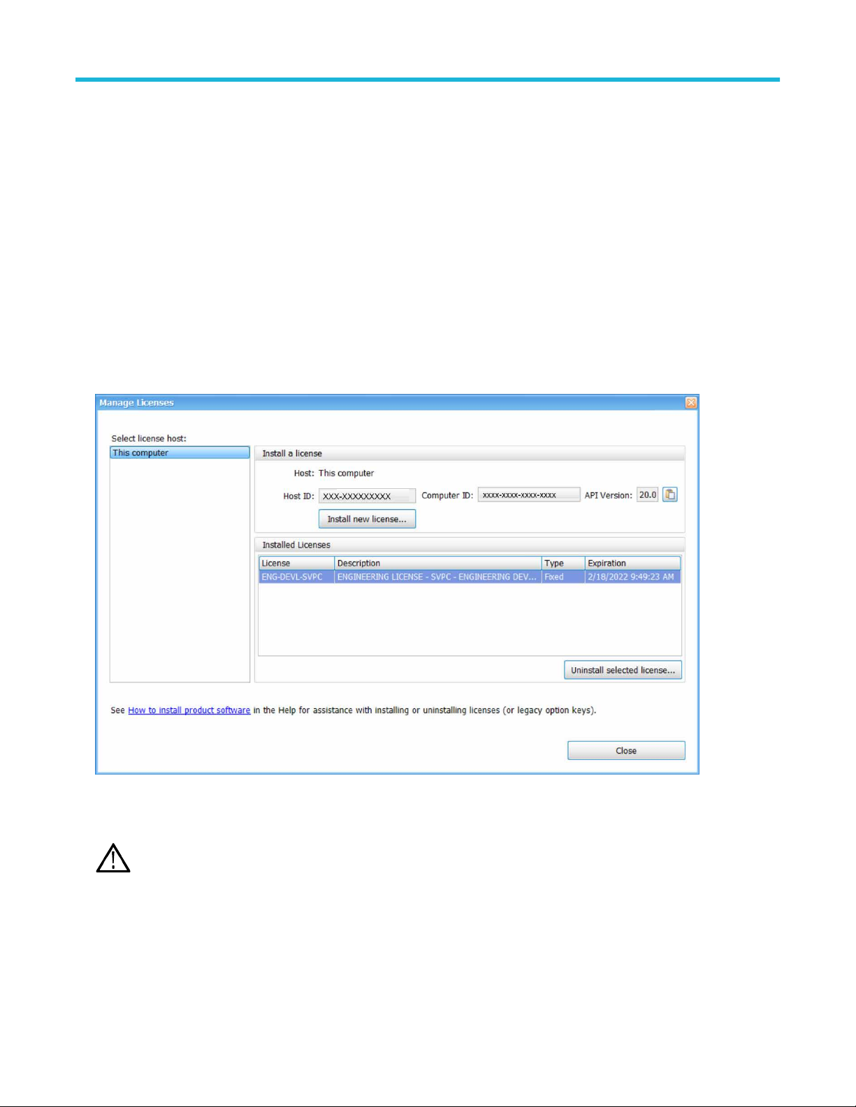
Get Started
You can view a list of the currently installed application licenses and options in your product as follows:
Select Tools > Licenses > Manage from the application’s main toolbar.
•
• Select Help > About Tektronix Real Time Signal Analyzer to view a list of the installed options.
How to install a license
Before installing an application license, you must first have purchased one and downloaded the license to your product or a portable
memory device. The following instructions include information about how to download and purchase licenses.
See Available application options on page 30
(Visit www.tek.com/products/product-license.)
1. Select Tools> Licenses > Manage to open the Manage Licenses window.
2. Select This computer or other license host from the list on the left side of the window
the ID for the selected host. Currently installed licenses associated with that host will also appear in the bottom right panel of the
window under Installed Licenses.
Note: Host ID, Computer ID, and API V
analysis plugins only Host ID is required.
3. If you already have a license file (*.lic) downloaded, click the Install new license button and navigate to the license you want to install,
and then click Open. The license will install and appear in the Installed Licenses list. This task is now complete.
4. If the license you want to install is in your T
a. Select the host on which you want to install the license from the Select license host list. For example, if you want to install the
license on the computer, select This computer. Notice that the Host ID field on the right will populate with the ID for the selected
host.
22
ersion fields are required for installing the 5GNR analysis plugin. To install other
ekAMS system account, do the following:
. Notice that the Host ID field will populate with
Page 23
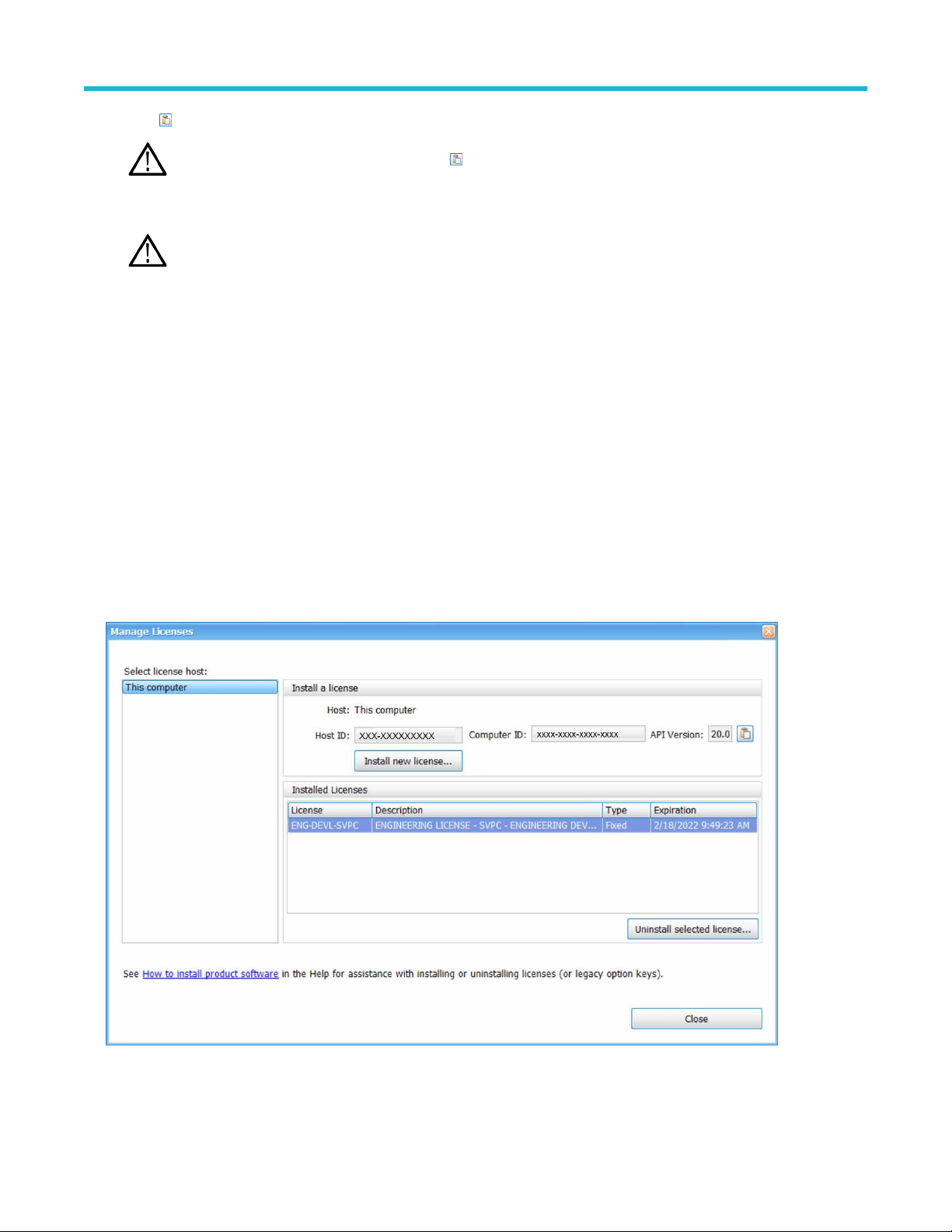
b. Click to copy the host ID.
Get Started
Note: T
o Install the 5GNR analysis plugin, Click
c. Navigate to the T
a link on this page www.tek.com/products/product-license.
Note: For the 5GNR analysis plugin, enter the Host ID and Computer ID.
d. Follow the instructions online to download the desired license file (*.lic).
e. Once the license is downloaded, perform step 3 on page 22 above.
5. If you do not have a license yet, do the following:
a. Using an Ethernet connection, navigate to www
b. Click on the Additional Options tab. This tab lists all available software license options.
c. Find the option you want, then click on the related link to download a free trail version.
d. Click on the related link to request a quote.
e. After your purchase is complete, you will receive instructions for creating a TekAMS account to access and manage your licenses.
Once your account is set up, perform step 4 on page 22 above.
ekAMS system, log in, and enter the host ID in the appropriate field. The Tek AMS system can be accessed from
.Tek.com/products and find your product.
to copy the Host ID, Computer ID, and API Version.
How to return a license
You can return (uninstall) a license from a particular product as follows:
1. Select Tools > Licenses > Manage to open the Manage Licenses window.
2. In the Manage Licenses window, select the license you want to return.
3. Click Uninstall selected license. The following window will appear
SignalVu-PC Vector Signal Analysis Software Help 23
.
Page 24
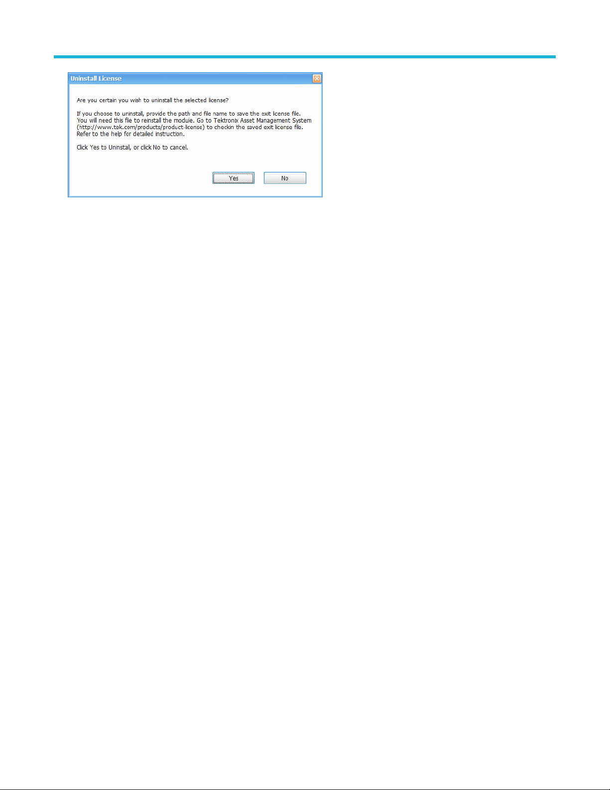
Get Started
4. Click Y
5. Save the exit license file to the desired location.
6. Click Close.
7. Navigate to your TekAMS account and check in the saved exit license file.
es to uninstall the license. You will then be prompted to save an exit license file. This is the file you will check into (return to)
your TekAMS account.
How to move a license to a different host
You can return a purchased license and then reassign it to a different host, as indicated below. See the Available application
options on page 30 topic for a list of available application licenses.
• Node locked license (NL): This license type can be reassigned no more than two times. This allows you to reassign the license in the
case of an upgrade to a new Windows platform, for example.
• Floating license (FL): This license type can be reassigned an unlimited number of times. When assigning a floating license, you need
to specify the host id and the duration the feature is to be enabled on the host. After the license expires, the feature is automatically
disabled on that host and the license in then available to be assigned to a different host.
• Free trial license (FT): This license type expires after 30 days.
See also:
www.tek.com/products/product-license
How to install a license on page 22
How to return a license on page 23
How to manage the 5GNR analysis license
After installing the SignalVu-PC 5GNR Analysis plugin, it needs to be activated on that instrument/PC/laptop. The activation requires an
activation code which is 20 digit alphanumeric characters separated by a hyphen between every four characters. The following topics give
procedure to activate or deactivate the 5GNR Analysis.
5GNR Analysis activation
1. Start the SignalVu-PC application.
2. On the Tools menu, click Manage 5GNR Analysis Activation…. The Manage 5GNR Analysis Activation dialog box appears.
24
Page 25
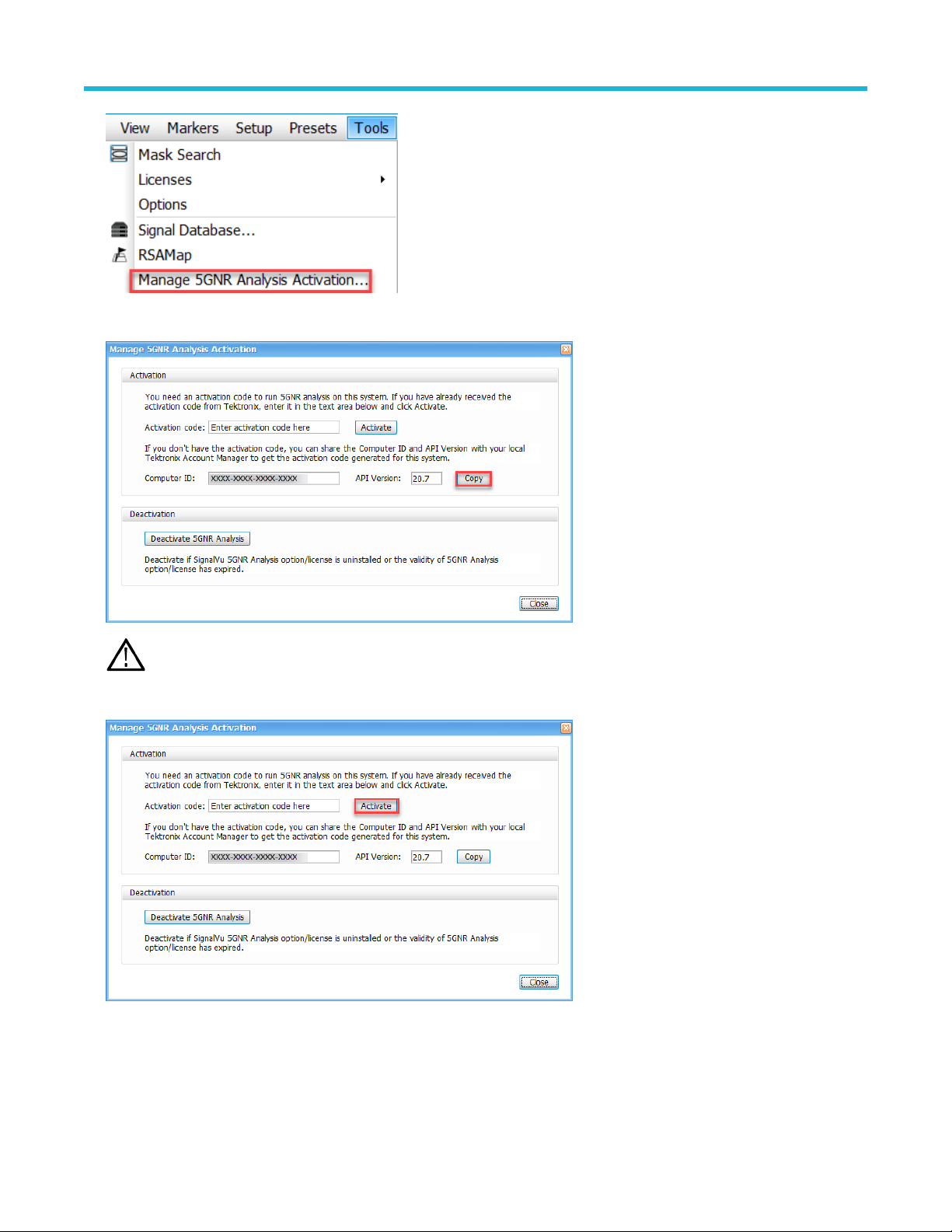
Get Started
3. If you do not have the activation code, under Activation, click Copy, and then close the Manage 5GNR Analysis Activation dialog
box.
Note: Share the Computer ID and API V
activation code generated for this system.
4. If you have the activation code, under Activation, in the Activation code box, enter the activation code that you received from
T
ektronix, and then click the Activate.
5. If you receive the “5GNR Analysis activation failed. Please enter a valid activation code.” message, click OK, and then contact your
local T
ektronix support or Account Manager to get the correct activation code.
ersion that you have copied with your local Tektronix account manager to get the
SignalVu-PC Vector Signal Analysis Software Help 25
Page 26
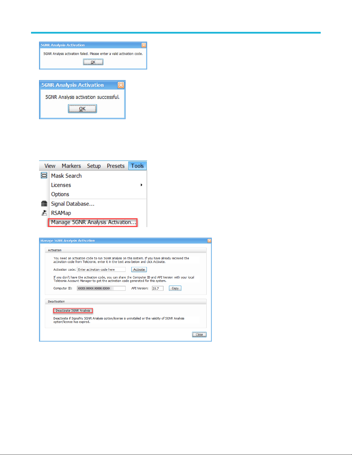
Get Started
6. If you receive the “5GNR Analysis activation successful” message, click OK.
7. Close the Manage 5GNR Analysis Activation dialog box and restart the
SignalVu-PC application.
5GNR Analysis de-activation
1. Start the SignalVu-PC application.
2. On the Tools menu, click Manage 5GNR Analysis Activation…. The Manage 5GNR Analysis Activation dialog box appears.
3. Under Deactivation, click Deactivate 5GNR Analysis.
4. Click OK and continue with 5GNR Analysis de-activation.
26
Page 27
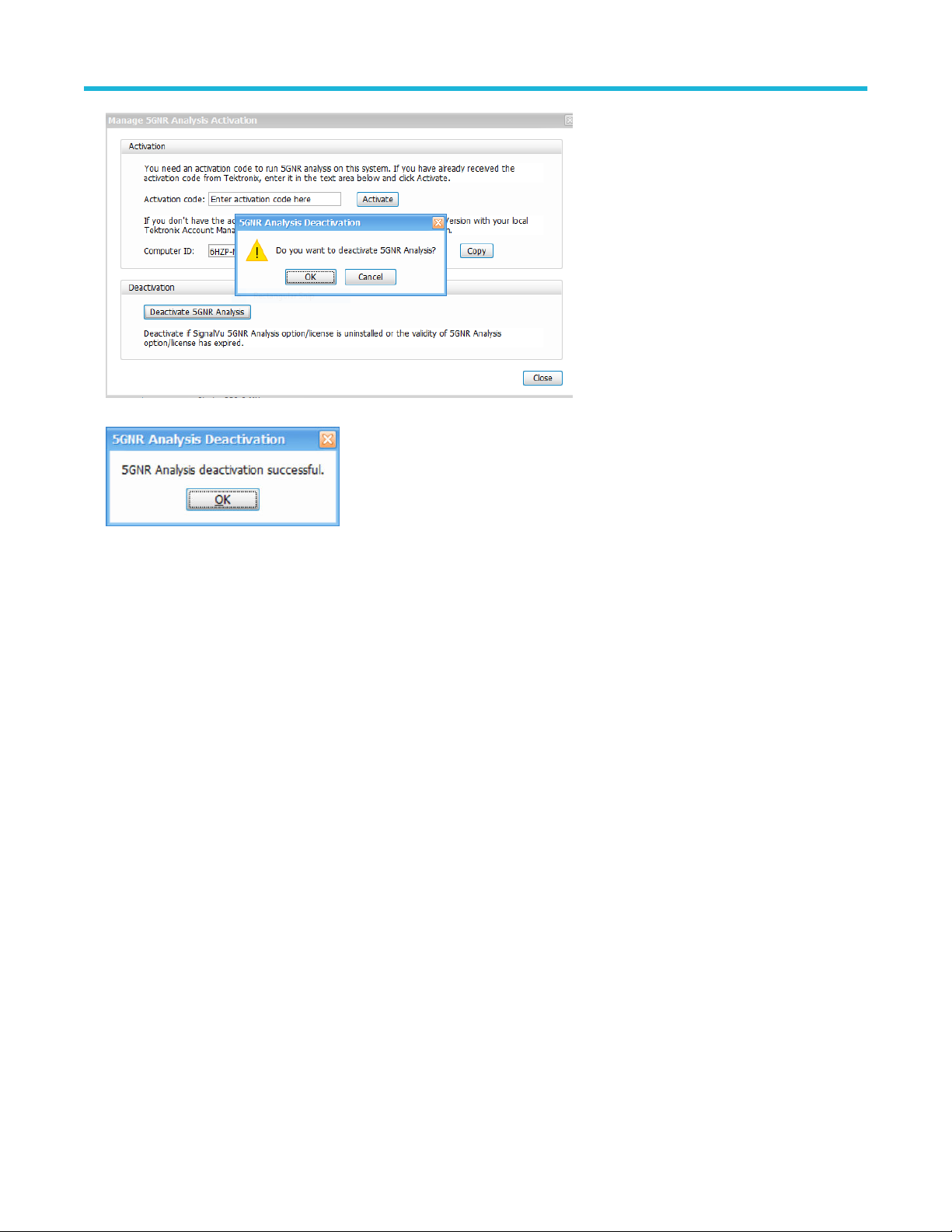
Get Started
5. If you receive the “5GNR Analysis deactivation successful” message, click OK, and then restart the
SignalVu-PC application.
How to activate legacy options (application licenses)
Activating options requires internet access. However, you can activate options on a PC that does not have internet access by using a
second PC that does have internet access to contact the license server and use it to download a license file. The license file can then be
transferred to the PC on which the option is to be activated. In order to use any options you have purchased for SignalVu-PC, you must
activate each option individually one of the following two ways:
To activate an option with Internet access
1. Launch the SignalVu-PC application.
2. Select Tools > Licenses > Legacy > Activate... to view the Activate Legacy License dialog.
3. In the dialog, select Auto.
SignalVu-PC Vector Signal Analysis Software Help 27
Page 28
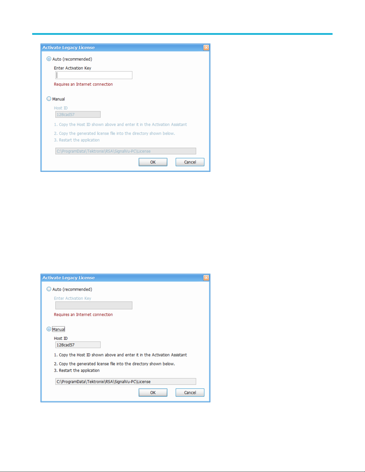
Get Started
4. In the Enter Activation Key text box, enter the option activation key provided when you purchased the option.
5. Click OK. SignalV
6. Repeat the steps above to activate each option, using the activation key specific to each option.
u-PC will contact the license server and install a license file provided by the license server.
To activate an option without Internet access
To activate options on a PC without internet access, you need use the Offline Activation Tool. The tool is provided with SignalVu-PC as a
separate installation file.
1. Launch the SignalVu-PC application.
2. Select Tools > Licenses > Legacy > Activate... to view the Activate Legacy License dialog.
3. In the dialog, select Manual.
rite down the Host ID shown in your Activate Legacy License dialog, and then click Cancel to close the window.
4. W
5. Install the Activation Assistant software on a PC that has internet access.
28
Page 29

Get Started
The Activation Assistant software is located at:
If you installed SignalVu-PC from a DVD or USB flash drive, navigate to the device, open the Offline Activation Tool folder, and run
•
the Setup file located there.
• If you downloaded SignalVu-PC from the Web, navigate to the location you extracted the installation files. Open the Offline
Activation Tool folder and run the Setup file located there.
6. Launch the Activation Assistant application and follow the instructions to generate a license file. Repeat this step for each option that
you have purchased. You will also need the option activation key you received.
Activation keys are specific to each option, therefore you must acquire a license file for each option purchased.
7. Copy the license file (or files) to the following location the PC on which SignalVu-PC is to be activated:
C:\ProgramData\Tektronix\RSA\SignalVu-PC\License
8. Restart the SignalVu-PC application.
How to activate options in free trial (evaluation) mode
If you don’t have a license for one (or any) SignalVu-PC options, you can activate each option in evaluation mode for 30 days. Trial
licenses are available at https://www.tek.com/product-software-series/signalvu-pc.
Note: Each option has its own evaluation period.
To activate an option in evaluation mode:
1. Launch SignalV
2. Launch SignalVu.
3. Select Tools > Licenses > Legacy > Manage... to view the Manage Legacy License dialog.
4. Select the option you want to evaluate, and then click the Start 30-day evaluation button.
The Current Status box will change to display the number of days remaining for evaluation. Repeat this procedure for each of the
options you wish to evaluate.
u-PC.
How to manage legacy option licenses
Options are licensed for use on a single PC. However, you can move SignalVu-PC and its options from one PC to another PC by
deactivating each option on the current installation and reactivating them on another PC. Each activated option needs to be deactivated as
follows:
1. Launch the application.
2. Select Tools > Licenses > Legacy > Manage... to view the Manage Legacy License dialog.
3. Use to the drop-down list under Option to select one of the options that is activated.
For example: OFDM Measurements (SignalVu-PC SVO).
4. Starting with each installed option, click Deactivate License. Continue selecting options and clicking Deactivate License until all the
options have been deactivated.
The SignalVu-PC options are now deactivated. You can now install the software on another PC and activate the options in the new
installation.
SignalVu-PC Vector Signal Analysis Software Help 29
Page 30
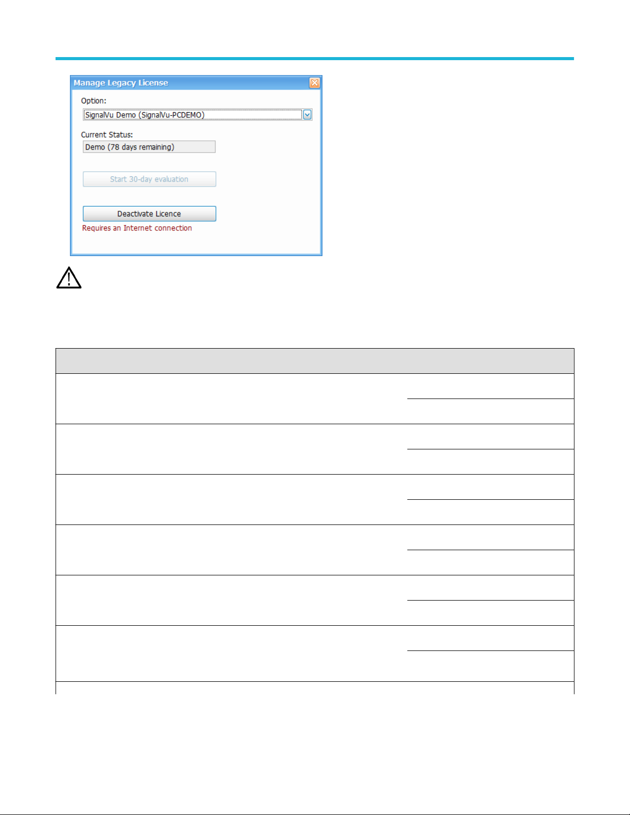
Get Started
ou can view already installed and activated options from the Tools > Licenses > Legacy > Manage... window.
Note: Y
Available application options
The following table shows available optional applications for SignalV
Application description Application (option) License type
AM/FM/PM/Direct Audio Analysis SVANL-SVPC Node Locked
Settling Time (frequency and phase) measurements SVTNL-SVPC Node Locked
General Purpose Modulation Analysis to work with analyzer of acquisition bandwidth ≤
40 MHz and MDO
General Purpose Modulation Analysis to work with analyzer of any acquisition bandwidth SVMHNL-SVPC Node Locked
800 MHz acquisition bandwidth (for frequencies > 3.6 GHz
(RSA7100 only)
u-PC.
SVAFL-SVPC Floating
SVTFL-SVPC Floating
SVMNL-SVPC Node Locked
SVMFL-SVPC Floating
SVMHFL-SVPC Floating
B800NL-SVPC Node Locked
B800FL-SVPC Floating
Pulse Analysis to work with analyzer of acquisition bandwidth ≤ 40 MHz and MDO
Pulse Analysis to work with analyzer of acquisition bandwidth less than or equal to 40MHz
and multi-channel analysis with 5/6 Series MSO; electronically downloaded canned software
Table continued…
30
SVPNL-SVPC Node Locked
SVPFL-SVPC Floating
Page 31

Application description Application (option) License type
Get Started
Pulse Analysis to work with analyzer of any acquisition bandwidth
Pulse Analysis to work with analyzer of any acquisition bandwidth and multi-channel analysis
with 5/6 Series MSO; electronically downloaded canned software
Phase Noise measurements
(RSA7100 only)
Advanced triggers (Frequency Mask, Density)
(RSA7100 only)
EMI Pre-compliance and Troubleshooting
(Includes CISPR detector support on RSA306B, RSA500 series, RSA600 series, and
RSA5000 series only)
SVPHNL-SVPC Node Locked
SVPHFL-SVPC Floating
PHASNL-SVPC Node Locked
PHASFL-SVPC Floating
TRIGHNL-SVPC Node Locked
TRIGHFL-SVPC Floating
EMCVUNL-SVPC Node Locked
EMCVUFL-SVPC Floating
Flexible OFDM Analysis SVONL-SVPC Node Locked
SVOFL-SVPC Floating
WLAN 802.11a/b/g/j/p measurements SV23NL-SVPC Node Locked
SV23FL-SVPC Floating
WLAN 802.11n measurements
(Requires SV23NL-SVPC or SV23FL-SVPC)
WLAN 802.11ac measurement to work with analyzer of acquisition bandwidth ≤ 40 MHz and
SV24NL-SVPC Node Locked
SV24FL-SVPC Floating
SV25NL-SVPC Node Locked
MDO
(Requires SV23NL-SVPC or SV23FL-SVPC and SV24NL-SVPC or SV24FL-SVPC)
WLAN 802.11ac measurement to work with analyzer of any acquisition bandwidth and MDO
(Requires SV23NL-SVPC or SV23FL-SVPC and SV24NL-SVPC or SV24FL-SVPC)
SV25FL-SVPC Floating
SV25HNL-SVPC Node Locked
SV25HFL-SVPC Floating
APCO P25 measurements SV26NL-SVPC Node Locked
SV26FL-SVPC Floating
Bluetooth measurements
1
SV27NL-SVPC Node Locked
SV27FL-SVPC Floating
Table continued…
1
Bluetooth is a registered trademark of Bluetooth SIG, Inc.
SignalVu-PC Vector Signal Analysis Software Help 31
Page 32

Get Started
Application description Application (option) License type
Bluetooth 5 measurements
1
(Requires SV27NL-SVPC or SV27FL-SVPC)
SV31NL-SVPC Node Locked
SV31FL-SVPC Floating
Mapping MAPNL-SVPC Node Locked
MAPFL-SVPC Floating
SignalVu-PC connection to the MDO4000B/C series oscilloscopes
Live connection and base SignalV
u-PC VSA measurements using the 5 or 6 Series MSO
Oscilloscope (with opt. SV-RFVT); electronically downloaded canned software
WLAN 802.11a/b/g/j/p/n/ac and option to connect to MDO4000B/C. Works with analyzer of
CONNL-SVPC Node Locked
CONFL-SVPC Floating
SV2CNL-SVPC Node Locked
analyzer of acquisition bandwidth ≤ 40 MHz and MDO.
(This option bundles the following: SV23NL-SVPC or SV23FL-SVPC, SV24NL-SVPC or
SV2CFL-SVPC Floating
SV24FL-SVPC, SV25NL-SVPC or SV25FL-SVPC, and CONNL-SVPC or CONFL-SVPC)
WLAN 802.11a/b/g/j/p/n/ac and Connect to 5/6 Series MSO (with opt. SV-RFVT) to work with
analyzer of acquisition bandwidth ≤ 40 MHz; electronically downloaded canned software
WLAN 802.11a/b/g/j/p/n/ac and option to connect to MDO4000B/C. Works with analyzer of
SV2CHNL-SVPC Node Locked
any acquisition bandwidth.
(This option bundles the following: SV23NL-SVPC or SV23FL-SVPC, SV24NL-SVPC or
SV2CHFL-SVPC Floating
SV24FL-SVPC, SV25HNL-SVPC or SV25HFL-SVPC, and CONNL-SVPC or CONFL-SVPC)
LTE Downlink RF measurements
2
SV28NL-SVPC Node Locked
SV28FL-SVPC Floating
5G NR Uplink/Downlink RF Power, Bandwidth, Demodulation, and Error Vector Magnitude
measurements
5GNRNL-SVPC Node Locked
5GNRFL-SVPC Floating
WiGig 802.11ad and 802.11ay measurements (only for offline analysis) SV30NL-SVPC Node Locked
SV30FL-SVPC Floating
EMI CISPR detectors SVQPNL-SVPC Node Locked
SVQPFL-SVPC Floating
Signal survey and classification SV54NL-SVPC Node Locked
SV54FL-SVPC Floating
Table continued…
2
TE is a trademark of ETSI.
L
32
Page 33

Application description Application (option) License type
Get Started
Playback of recorded files
(RSA500A series and RSA600A series only)
Streaming data to RAID and 40 GbE
(RSA7100 only)
Streaming IQ data to a custom API application
(RSA7100 only)
Return loss, VSWR, cable loss, and distance to fault
(RSA500A series and RSA600A series only)
Education-only version of all modules for SignalVu-PC EDUFL-SVPC Floating
Tip: See the Features by product on page 33 topic for more information.
SV56NL-SVPC Node Locked
SV56FL-SVPC Floating
STREAMNL-SVPC Node Locked
STREAMFL-SVPC Floating
CUSTOM-APINL-
SVPC
SV60NL-SVPC Node Locked
SV60FL-SVPC Floating
Node Locked
Features by product
The following table lists a subset of features that may or may not be available for your analyzer when connected to SignalV
means the feature is available with the specified product.A n X means the feature is planned for a future release. Some of these features
require specific options be installed. You can view a list of options for SignalVu-PC. Available application options on page 30
u-PC. A “√”
Feature RSA300 Series RSA500 Series RSA600 Series RSA7100 Series
Audio demodulation
(listening)
DPX Spectrogram
(DPXogram)
Fast Frame √
Frequency Mask Trigger √
Phase Noise (Option
PHAS-SVPC)
(RSA7100 only)
DPX Density Trigger √
Time Qualified Trigger √
Internal GPS √ √ √
Playback of recorded files
(Option SV56-SVPC)
Playback of recorded files
(external application)
Table continued…
√ √ √
√ √ √ √
√
√ √ √
√ √ √ √
SignalVu-PC Vector Signal Analysis Software Help 33
Page 34

Get Started
Feature RSA300 Series RSA500 Series RSA600 Series RSA7100 Series
Tracking generator and
return loss, VSWR, cable
loss, and distance to fault
(Option 04 with SV60SVPC)
√ √
Available product documentation
In addition to this Help, the following documents are available. For the most up to date documentation, visit the T
www.tektronix.com/manuals.
ektronix Web site
Product documents
• SignalVu-PC Quick Start User Manual (Tektronix part number 077-1024-XX). This PDF document explains how to install and activate
the SignalVu-PC software. The instructions also provide a brief overview of the SignalVu-PC interface to get you started. It is available
for download at www.Tek.com/manuals and can also be accessed from the Help menu in the application.
• SignalVu-PC Programmer Manual (077-0721-XX). This PDF document provides detailed descriptions of the remote commands for
the SignalVu-PC software and explains how to use the programming interface for SignalVu-PC.
• SignalVu-PC Printable Help Document (PDF) (077-0720-XX). A PDF file version of this Help that can be printed.
• RSA500 Series Installation and Safety Manual (Tektronix part number 071-3452-XX). This document explains how to install the
instrument and battery, connect, and prepare the RSA500 Series instruments for use. It is available for download at www.Tek.com/
manuals and is shipped as a printed manual with your instrument.
• WFM200BA Rechargeable Battery Pack Instructions (Tektronix part number 075-1041-XX). This document contains information for
handling, storing, maintaining, recycling, and transporting the WFM200BA Li-Ion rechargeable battery pack. For use with the RSA500
Series instruments.
• WFM200BC External Battery Charger Instructions (Tektronix part number 071-1042-XX). This document describes how to use the
WFM200BC external battery charger to recharge the WFM200BA Li-Ion battery pack. For use with the RSA500 Series instruments.
• RSA600 Series Installation and Safety Manual (Tektronix part number 071-3460-XX). This document explains how to install,
connect, and prepare the RSA600 Series instruments for use. It is available for download at www.Tek.com/manuals and is shipped as
a printed manual with your instrument.
• RSA306B Installation and Safety Manual (Tektronix part number 071-3483-XX). This document explains how to install, connect, and
prepare the RSA306B instrument for use. It is available for download at www.Tek.com/manuals and is shipped as a printed manual
with your instrument.
• RSA7100 Quick Start User Manual (Tektronix part number 071-3504-XX). This document explains how to install, connect, and
prepare the RSA7100 instrument for use. It also contains some basic operation procedures to get you started. It is available for
download at www.Tek.com/manuals and is shipped as a printed manual with your instrument.
• If you are using an RSA306B, RSA500 Series, RSA600 Series, RSA7100, or MDO4000/B or C Series instrument with SignalVu-PC,
you can find more product related documents than those listed above online at www.Tek.com/manuals.
The most recent versions of the product documentation, in PDF format, can be downloaded from www.Tek.com/manuals. You can find the
manuals by searching on the product name and selecting the Manuals filter.
Available demonstration guide and handbook
Available for download on www.Tek.com.
• 5GNR
There are two documents, 5G New Radio Demonstration Guide and 5GNR AWG Handbook.
In the 5G New Radio Demonstration guide, you will learn how to analyze Uplink and Downlink frames of 5G signal using the 5GNR
analysis plugin installed on SignalVu analysis software.
34
Page 35

Get Started
In the 5GNR AWG handbook, you will learn how to create 5GNR waveforms in uplink or downlink directions, single or multiple carriers
at the desired center frequency
.
Available demonstration guides
Available for download on www.Tek.com.
• Interference Hunting
This demonstration guide shows how spectrum management operators can discover and capture signals of interest, using Swept DPX,
with as short as 100 us duration and 100% Probability of Intercept (POI) that would be easily hidden with traditional instruments. DPX
can now be used to sweep across the entire instrument’s frequency range. With traditional swept spectrum analyzers and vector signal
analyzers, only 1 spectrum trace is displayed. With Swept DPX, the instrument dwells at each step to build the entire spectrum with
thousands of spectrums displayed in a way that is usable for the engineers or spectrum managers.
• EMC Precompliance and EMC testing
With this demonstration guide, you will explore what you can do with the Tektronix USB spectrum analyzer with EMCVu. Applications
range from simple frequency / amplitude measurements of RF signals to real-time and modulation analysis that provide you with a
complete system view of your device under test.
• Signal Locating
RSA Map tool in the Tektronix RSA/SignalVu-PC/SPECMON lets you use an on-screen map to record the location and value of
RSA/SignalVu-PC/SPECMON measurements. With RSA Map you can use a GPS receiver to automatically position measurements at
your current location on maps with geophysical reference information. The example in this Demo guide uses a free online mapping
source OpenStreetMap to capture maps. OpenStreetMap is a collaborative project to create a free editable map of the world. It can
capture a map anywhere in the world and can export it in its native format, bitmap image, and embeddable HTML.
• LTE
In this demonstration guide, you will learn how to make LTE downlink measurements either using RSA demo board for base station
transmitter tests, or using an antenna for the over-the-air signal analysis.
• 5GNR
There are two documents, 5G New Radio Demonstration Guide and 5GNR AWG Handbook.
In the 5G New Radio Demonstration guide, you will learn how to analyze Uplink and Downlink frames of 5G signal using the 5GNR
analysis plugin installed on SignalVu-PC analysis software.
In the 5GNR AWG handbook, you will learn how to create 5GNR waveforms in uplink or downlink directions, single or multiple carriers
at the desired center frequency.
• Internet of Things (IoT)
In this demonstration guide, you will learn how to use Tektronix USB RSA to make the standard certification tests on IoT devices.
Wireless technology standards are needed to ensure that products can interoperate within the ecosystem where they will be deployed.
There are a number of technologies to choose from, including Wi-Fi®, Bluetooth®, ZigBee®, and LoRa®. However, to adhere to the
standard, new products will need to meet qualification as defined per the standard selected. Failing qualification can mean design turns
that will delay the final product release and draw additional significant development cost.
• SignalVu-PC
This demonstration guide is designed to help you understand the benefits of SignalVu PC for analysis of waveforms captured
by Tektronix DPO/DSA/MSO Series digital oscilloscopes, MDO4000 Multi-Domain Oscilloscopes and Tektronix Real Time Signal
Analyzers. Applications include: CW Tone, Wideband Radar, Hopping Waveforms, Wideband Monudaltion, Multi-domain oscilloscope
acquisitions, AM/FM/PM/Audio Analysis, Signal Monitoring with RTSA waveforms, and WLAN 802.11ac Signal Analysis.
Video tutorials
You can browse the Tektronix YouTube channel (www.youtube.com/user/tektronix) to find video tutorials about various topics related to
your product. You can also subscribe to the Tektronix YouTube channel to keep up with new postings.
SignalVu-PC Vector Signal Analysis Software Help 35
Page 36

Get Started
Searching for topics
For example, you can watch a video tutorial about performing basic EMI testing with a spectrum analyzer
and connect to an MDO4000C oscilloscope. To find a video on a topic, do the following. The following image shows you what the Tektronix
YouTube Channel looks like.
1. Click on the search icon located just above the video you see when the page first loads.
Note: This icon allows you to search the T
page allows you to search all of YouTube.
2. T
ype in the key phrase you are looking for in the search field. For example, “WLAN”.
3. Click the search icon to start the search.
4. Videos related to the topic will appear. Click a video to view it.
ektronix YouTube channel specifically. The search icon located at the top of the
, or how to use WLAN presets
Orientation
This section contains information about the SignalVu-PC software user interface.
Selecting Files for Analysis
The SignalVu-PC software can analyze waveform files saved by Tektronix oscilloscopes and real-time signal analyzers. SignalVu-PC can
open several file types, including .wfm, .tiq, .iqt and .mat files. For more detailed information on opening the supported file types, see.
Recalling waveforms with SignalVu-PC on page 791
Right-Click Action Menu
You can change marker settings and how waveforms are displayed by using the right-click Actions menu.
36
Page 37

To use the right-click Actions menu, right-click in the graph area.
Icon Menu Description
Select Selects markers and adjusts their position.
Span Zoom Zooms the graph area about the selected point. Right-click in the graph display
at a point of interest and drag to increase or decrease the span about the point
of interest. Span Zoom adjusts the span control.
Get Started
CF Pan Adjusts the Center Frequency according to horizontal movement.
Zoom Adjusts horizontal and vertical scale of the graph. The first direction with
enough movement becomes the primary scale of adjustment. Adjustment
in the secondary direction does not occur until a threshold of 30 pixels of
movement is crossed.
Dragging to the left or down zooms out and displays a smaller waveform
(increases the scale value). Dragging to the right or up zooms in and displays
a larger waveform (decreases the scale value).
Pan Adjusts horizontal and vertical position of the waveform. The first direction with
enough movement becomes the primary direction of movement. Movement
in the secondary direction does not occur until a threshold of 30 pixels of
movement is crossed.
- Reset Scale Returns the horizontal and vertical scale and position settings to their default
values.
- Marker to peak Moves the selected marker to the highest peak. If no marker is turned on, this
control automatically adds a marker.
- Add marker Defines a new marker located at the horizontal center of the graph.
- All markers off Removes all markers.
SignalVu-PC Vector Signal Analysis Software Help 37
Page 38

Get Started
SignalVu-PC Markers Menu
The SignalV
marker to a different trace and pan the trace to place the marker at the measurement frequency.
Icon Menu Description
- Pan to marker Adjusts horizontal position of the waveform to locate the selected marker at
- Assign to trace Assigns the selected marker to Trace 1, Trace 2, Trace 3 or the Math trace. A
u-PC Markers menu appears when you right-click on a marker. The SignalVu-PC Markers menu enables you to assign a
the measurement frequency
trace must be enabled to assign a marker to it.
.
38
Page 39

Elements of the Display
General application window areas. The main areas of the application window are shown in the following figure.
Get Started
Note: If values or buttons on the application UI become truncated or displaced, you may need to adjust the Microsoft Windows
display settings or custom DPI percentage setting.
Specific elements of the application display window. Specific elements of the display are shown in the following figure. More detailed
information is available in the Main menu overview on page
804 section.
SignalVu-PC Vector Signal Analysis Software Help 39
Page 40

Get Started
Ref number Setting Description
1 Recall Displays the Open window in order to recall setup files, acquisition data files, or trace files.
2 Save Opens the Save As dialog in order to save setup files, pictures (screen captures),
acquisition data files, or export measurement settings.
3 Undo/Redo Undoes or redoes the previous edit to a display or measurement settings, a preset, or a
measurement change.
4 Displays Opens the Select Displays dialog box so that you can select measurement displays.
5 Settings Opens the Settings control panel for the selected display. Each display has its own control
panel.
6 Trigger
(Only available when
connected to an RSA306,
RSA306B, RSA500A series,
and RSA600A series,
RSA7100 series, or
MDO4000B/C.)
Table continued…
Opens the Trigger control panel so that you can define the instrument trigger settings.
40
Page 41

Get Started
Ref number Setting Description
7 Acquire Opens the Acquire control panel, which displays the Sample Rate and Record length of the
recalled waveform file.
8 Analysis Opens the Analysis control panel so that you can define the analysis settings such as
frequency
9 Amplitude Opens the Amplitude control panel so that you can define the Reference Level, configure
internal attenuation, and specify external gain/loss corrections.
10 GNSS/Antenna Opens the GNSS/Antenna control panel so that you can configure and activate an internal
or external GNSS receiver and antenna.
11 Audio Demodulation Opens the Audio control panel so that you can define the audio demodulation settings for
the RSA306, RSA306B, RSA500A series, RSA600A series, and RSA7100.
12 Recording Opens the Recording control panel so that you can record and configure recording of
signals. For detailed information, see the Setup Menu on page 814 topic.
13 Favorite User Presets Click to select from a list of custom favorite User presets and load the selected preset. For
more detailed information, see the Make a User preset on page 46 topic.
, analysis time, and units.
14 Main menu bar Contains access to menus. For detailed information, see the Main menu
overview on page 804 topic.
15 Preset Recalls the Presets on page 42 preset.
16 Replay Runs a new measurement cycle on the existing acquisition data record using any new
settings. See the Replay Menu on page 714 topic for more details.
17 Run
and
Run/Stop toolbar
(Only available when
connected to an RSA306,
RSA306B, RSA500A series,
and RSA600A series,
RSA7100 series, or
MDO4000B/C.)
Table continued…
• Run menu and Run/Stop toolbar
Starts and stops data acquisitions and specifies the run conditions. For example, if
you select Single in the Run/Stop toolbar (or Run Single in the Run menu), a single
measurement cycle is run. If you select Continuous in the Run/Stop toolbar (or Run
Continuous in the Run menu), the data acquisition runs until stopped.
• Run menu
The Run menu also includes Resume and Abort.
Resume restarts data acquisition, but does not reset accumulated results, such as Average
or MaxHold. This allows you to stop acquisitions temporarily, then continue.
Abort immediately halts the current acquisition/measurement cycle. In-process
measurements and acquisitions are not allowed to complete.
See the Run Menu on page 813 topic for more details.
SignalVu-PC Vector Signal Analysis Software Help 41
Page 42

Get Started
Ref number Setting Description
18 The Edit Favorites icon allows you access the below menu, which allows you to
edit the contents of the Favorites bar
menus on page 819 topic.
. For more information, see the Favorites bar
Restoring Default Settings
T
o restore the software to its factory default settings:
1. Select Presets > Preset Options.
2. In the Presets tab of the Options control panel, click to the view the Preset type drop down menu and select Main.
3. Click to the view the Presets drop down menu and select Original.
4. Click the red X icon in the top right corner of the Options control panel to close the panel.
5. Select Presets > Main from the menu bar to return the software to its original factory default settings.
Note: Y
ou can also click the Preset button on the right-hand side of the menu bar to load the Main preset.
Presets
Main menu bar: Presets
u-PC includes a set of standard configurations that are tailored to specific applications or types of analysis. These configurations,
SignalV
referred to as Presets, open selected displays and load settings that are optimized to address specific application requirements. You can
also make your own User presets to fit your application. Any User preset can be added to the Favorites bar, enabling one-button access to
your most used setups.
42
Page 43

Get Started
Preset Options
Select the Presets > Preset Options menu to open the Options control panel. Once you have chosen these settings, you can access any
preset or list of presets from Presets on the menu bar
• Preset type: Select the Preset type.
• Presets: Select the specific preset you want to display for the selected preset type.
• Preset action: Selecting a preset from the Preset drop down menu results in one of two actions depending on which item you choose
in the Preset action list: Recall selected preset will immediately execute a preset when it is selected from the Presets menu. Show
list will display a list of presets subtypes from which you can then select the preset you want to recall.
.
Available Presets
Select Presets from the menu bar to access the presets shown in the following table. Preset subtypes are managed in the Presets >
Preset Options on page 43 menu.
Preset Description
Main
Current This Preset sets the analyzer to display a Spectrum display with
settings appropriate for typical spectrum analysis tasks.
Restoring Default Settings on page 42 This Preset is the original factory preset used with your original
u-PC software. This version of the factory preset is included
SignalV
to allow you to maintain compatibility with existing remote control
software.
DPX primer on page 71
(Only available when an RSA306, RSA306B, RSA500A series, RSA600A series, or RSA7100 series is connected.)
Open the DPX display The Open the DPX display opens the DPX display without closing
existing displays.
Swept The DPX Swept Preset displays the DPX Spectrum display with the
span set to maximum and the center frequency set to 1/2 the span.
Real Time The DPX Real Time Preset displays the DPX Spectrum display
with the center frequency set to 1.5 GHz and the span set to the
maximum available real-time bandwidth.
Standards
WLAN Measurements Overview on page 269 This preset sets the analyzer to display the WLAN Summary, WLAN
Constellation, and SEM displays. After you select the standards
and bandwidth, the software configures these displays to apply the
parameters appropriate for typical WLAN analysis tasks.
Table continued…
SignalVu-PC Vector Signal Analysis Software Help 43
Page 44

Get Started
P25 Overview
Overview on page 586 This preset loads a set of Bluetooth displays and test setup to
LTE Overview on page 499 This preset loads a set of LTE displays and a test setup,
5GNR Analysis This preset loads a set of 5GNR displays and a test setup,
Overview of 802.11ad and 802.11ay on page 299 This preset loads a set of standards (Control PHY and Single carrier
Application
on page 464 This preset sets the analyzer to display the P25 MCPR, Summary,
P25 Constellation, and Time Overview displays. After you select
the standard and modulation type, the software configures these
displays to apply the parameters appropriate for typical P25
analysis tasks.
perform Bluetooth SIG RF tests. The software configures these
displays to apply the parameters appropriate for Bluetooth analysis
tasks.
frame structure, and channel bandwidth to perform LTE tests.
The software configures these displays to apply the parameters
appropriate for LTE analysis tasks.
frame structure, and channel bandwidth to perform 5GNR tests.
The software configures these displays to apply the parameters
appropriate for 5GNR analysis tasks.
PHY) for 802.11ad and 802.11ay for offline analysis.
Application Preset: Modulation Analysis on page 48 The Modulation Analysis setup application preset provides you with
the most common displays used during modulation analysis. Only
present when Option 21 is installed.
Application Preset: Pulse Analysis on page 48 The Pulse Analysis application preset provides you with the most
common displays used during pulse analysis, and makes changes
to the default parameters to settings better optimized for pulsed
signal analysis.
Application Preset: Phase Noise on page 48 The Phase Noise application preset opens the Phase Noise display,
and makes changes to the default parameters to settings better
optimized for phase noise analysis. Only present when a RSA7100
connected with Option PHAS-SVPC installed.
Application Preset: Time-Frequency Analysis on page 49 The Time-Frequency preset configures the analyzer with settings
suited to analyzing signal behavior over time.
Application Preset: Spectrum Analysis on page 49 The Spectrum Analysis application preset provide you with the
settings commonly used for general purpose spectrum analysis.
Application Preset: Spur Search Multi Zone 9k-1GHz on page 50 The Spur Search application preset sets the analyzer to display all
spurs that exceed the Threshold and Excursion values for the entire
9 kHz through 1 GHz range.
User (Favorites)
Table continued…
44
Page 45

Get Started
User Preset 1
User Preset 2 This preset sets the analyzer to show the Spurious display. Settings
Interference Hunting This preset sets the analyzer to show the DPX and Signal Strength
Other user presets User presets you create and save will appear in the Preset drop
This preset sets the analyzer to show these displays: Frequency
ime, Time Overview, Spectrogram, and Spectrum. Settings
vs T
commonly used for general purpose analysis are loaded.
commonly used for spur analysis are loaded.
displays.
down menu of the User Presets window. Any User preset that you
have designated as a Favorite will be marked with an *.
Recalling a Preset
o recall a preset, select Presets and then the desired preset type.
T
ou can set which presets to recall from the Presets > Preset Options on page 43 control panel.
Note: Y
Note: Y
ou can also click the Preset button on the top right side of the menu bar to load the Main preset.
User (Favorites) Presets
Select the Presets > User (Favorites) menu to open the User Presets window
presets provided with the software.
. The Presets drop-down list shows the three default user
• User Preset 1: Sets up the Spectrum, T
• User Preset 2: Sets up the Spurious display.
• Interference Hunting: Sets up the DPX and Signal Strength displays.
SignalVu-PC Vector Signal Analysis Software Help 45
ime Overview, Spectrogram, and Frequency vs Time displays.
Page 46

Get Started
Make a User preset
ou can add your own User presets to the list that appears in the User Presets dialog box as follows:
Y
1. Select Save As from the File menu to open the Save As dialog box.
2. Select to save to C:\SignalVu-PC Files\User Presets.
3. Enter a file name. The name you give the file will appear in the User Presets dialog box list.
4. Select the .Setup file type file from the Save as type drop-down list.
5. Click Save.
Make a User preset a Favorite preset. You can place one or more User presets on the Favorites bar as a Favorite preset for quick
access. Do this as follows:
1. Select Presets > User to open the User Presets window.
2. Select the desired preset from the Presets drop-down list.
3. Click the Add Favorite button. The preset will now have an * next to it. You can do this for more than one preset.
4. If desired, add a note for this preset in the Notes field and then click the Save button. Whenever you recall this preset, this note will
appear in a separate window
5. Click the OK button in the User Presets window
6. Click on the
7. When you are ready to recall a Favorite preset, click and select the preset from the list that appears.
8. T
o remove a Favorite preset, select it from the User Presets window and click the Remove Favorite button. The * should disappear
from the list.
46
icon on the Favorites bar and you will see the recently added Favorite preset listed.
, as shown below.
.
Page 47

Standards Presets
Get Started
The Standards presets allow you to recall preconfigured displays for the standards that you select. Y
standards groups.
• WLAN: The IEEE wireless LAN (WLAN) standards specify the wireless interface between two wireless clients or a wireless client and a
base station. The WLAN presets allow you to access displays preconfigured for the WLAN standards and bandwidths you select.
Note: More information is available about WLAN standards WLAN Measurements Overview on page
watch a video tutorial about WLAN Presets at www.youtube.com/user/tektronix. Click here for information about searching the
Tektronix YouTube channel for videos.
• P25: The Project 25 (P25) TIA-102 standards specify the design of interoperable digital two-way wireless communications products.
The P25 presets allow you to access displays preconfigured for the P25 standards you select. You can choose either the Phase 1
(FDMA) standard or the Phase 2 (TDMA) standard.
Note: More information is available about P25 standards #unique_29/unique_29_Connect_42_B-Overview on page 464.
• Bluetooth: The Bluetooth standards specify short range RF signals. The Bluetooth presets allow you to access displays preconfigured
for the specific Bluetooth standards you select: Basic Rate, Low Energy
Note: More information is available about Bluetooth standards Bluetooth Analysis.
• L
TE: The LTE standards ensure that the RF signals meet 3GPP measurements specifications. The LTE presets test setups load
pre-configured displays and control setting as suggested by the selected standard to accelerate the test setup of the analyzer.
Note: More information is available about LTE standards and test setups on page 499.
, and Enhanced Data Rate (EDR).
ou can select from the following
269. You can also
• 5GNR: The 5GNR standards ensure that the RF signals meet 3GPP measurements specifications. The 5GNR presets test setups load
pre-configured displays and control setting as suggested by the selected standard to accelerate the test setup of the analyzer
Note: More information is available about 5GNR standards and test setups 5GNR Overview .
• 802.1
SignalVu-PC Vector Signal Analysis Software Help 47
1ad and 802.11ay: Supports the set of standards for 802.11ad (Control PHY and Single carrier PHY) and for 802.11ay (single
carrier PHY at RF up to 70 GHz in DPO70000 DX series oscilloscopes, the DPO70000SX (with ATI) series oscilloscopes, and on
.
Page 48

Get Started
personal computers running SignalVu-PC for offline analysis. The ATI oscilloscope supports real time data analysis at RF, without any
downconverters.
Note: More information is available about 802.1
1ad and 802.11ay standards 802.11ad and 801.11ay Overview.
Application Preset: Modulation Analysis
The Modulation Analysis application preset opens the following displays:
•
DPX display: Shows you a continuous spectrum monitoring of the specified carrier frequency.
• Signal Quality: Shows a summary of modulation quality measurements (EVM, rho, Magnitude Error, Phase Error, and others).
• Constellation: Shows the I and Q information of the signal analyzed in an I vs Q format.
• Symbol Table: Shows the demodulated symbols of the signal.
To use the Modulation Analysis preset (assuming the Preset action is set to Show list in the Presets tab of the Options control panel):
1. Select Presets > Application. Select Modulation Analysis and then click OK.
2. Set the measurement frequency. Your signal should appear in the DPX display.
3. Set the reference level so that the peak of your signal is about 10 dB below the top of the DPX display.
4. Set the modulation parameters for your signal. This includes the Modulation Type, Symbol Rate, Measurement Filter, Reference Filter,
and Filter Parameter. All of these settings are accessed by selecting Tools > Settings.
For most modulated signals, the Modulation Analysis application preset should present a stable display of modulation quality. Additional
displays can be added by selecting Setup > Displays, and other settings can be modified to better align with your signal requirements.
Application Preset: Phase Noise
The Phase Noise application preset opens the Phase Noise display. (Only available on the RSA7100 with Option PHAS-SVPC installed.)
To use the Phase Noise preset (assuming the Preset action is set to Show list in the Presets tab of the Options control panel):
1. Select Presets > Application. Select Phase Noise and then click OK.
2. Set the center frequency. Your signal should appear in the Phase Noise display.
3. Set the reference level so that the peak of your signal is about 10 dB below the top of the DPX display.
4. Set the modulation parameters for your signal. This includes the Modulation Type, Symbol Rate, Measurement Filter, Reference Filter,
and Filter Parameter. All of these settings are accessed by selecting Tools > Settings.
Application Preset: Pulse Analysis
The Pulse Analysis application preset opens the following displays:
• DPX: The DPX display is opened with the maximum available span.
• Time Overview: Shows amplitude vs. time over the analysis period.
• Pulse Table: This shows a full report for the user-selected pulse measurements. If you want to clear the Pulse Table results for a new
acquisition, open the Time Overview window and select Autoscale. This causes the pulse table to refresh.
• Pulse Trace: Shows the trace of the selected pulse and a readout of the selected measurement from the pulse table.
• Pulse Cumulative Histogram: Shows a histogram that support statistics over multiple acquisitions. It shows basic pulse measurements
and has user definable bins for the cumulated pulses. It provides detailed information about the bins and its content.
48
Page 49

Get Started
• Pulse Cumulative Statistics Table: Shows a statistics table that provides information on Standard Deviation, Average, Max, and Min
ferent acquisitions.
over dif
• Pulse-Ogram: Shows a correlated Amplitude Time vs Time and frequency vs time display, where Y is pulse parameter, X is pulse
duration, and Z is number of pulses. It shows you a definable number of stacked pulses in amplitude versus time (reference being
the trigger time), as well as in amplitude versus frequency. This display will also show the information as an 'ogram, where the pulse
number is being scanned over time.
You can make a selected pulse and measurement appear in the Pulse Trace display by highlighting it in the Pulse Measurement Table.
Key pulse-related parameters that are set by the Pulse Analysis application preset are:
• Measurement Filter: No Filter-Max BW
• Measurement Bandwidth: This is set to the maximum real-time bandwidth of the instrument.
Note: The label on the “Measurement Bandwidth” setting is just “Bandwidth”. Like the main instrument Preset command and
the other application presets, the Pulse Analysis application preset also sets most other instrument controls to default values.
• Analysis Period: This is set to 2 ms to ensure a good probability of catching several pulses for typical signals.
•
Power threshold to detect pulses: This is set to –10 dBc.
• Minimum OFF time between pulses: This is set to 400.000 ns to ensure a good probability of catching several pulses for typical
signals.
• Max number of pulses: Check this box to limit the number of pulses to measure.
To use the Pulse Analysis preset (assuming the Preset action is set to Show list in the Presets tab of the Options control panel):
1. Select Presets > Application. Select Pulse Analysis and then click OK.
2. Set the Center Frequency control to the carrier frequency of your pulsed signal.
3. Set the Reference Level to place the peak of the pulse signal approximately 0-10 dB down from the top of the Time Overview display.
You may need to trigger on the signal to get a more stable display. This is set up in the Trigger control panel. (“Trig” button). Using the
Power trigger type with the RF Input source works well for many pulsed signals.
4. Set the Analysis Period to cover the number of pulses in your signal that you want to analyze. To do this, click in the data entry field of
the Time Overview window and set the analysis length as needed.
Application Preset: Spectrum Analysis
The Spectrum Analysis application preset opens a Spectrum display and sets several parameters. The Spectrum Analysis preset sets the
analyzer as follows.
• Spectrum Analysis : Sets the frequency range to maximum for the analyzer, and sets the RF/IF optimization to Minimize Sweep
Time.
To use the Spectrum Analysis preset (assuming the Preset action is set to Show list in the Presets tab of the Options control panel):
1. Select Presets > Application. Select Spectrum Analysis and then click OK.
2. Set the measurement frequency using the front-panel knob or keypad.
3. Adjust the span to show the necessary detail.
Application Preset: Time-Frequency Analysis
The Time-Frequency Analysis application preset opens the following displays:
• Time Overview: Shows a time-domain view of the analysis time ‘window’.
SignalVu-PC Vector Signal Analysis Software Help 49
Page 50

Get Started
• Spectrogram: Shows a three-dimensional view of the signal where the X-axis represents frequency, the Y-axis represents time, and
color represents amplitude.
Frequency vs. Time: This display's graph plots changes in frequency over time and allows you to make marker measurements of
•
settling times, frequency hops, and other frequency transients.
• Spectrum: Shows a spectrum view of the signal. The only trace showing in the Spectrum graph after selecting the Time-Frequency
Analysis preset is the Spectrogram trace. This is the trace from the Spectrogram display that is selected by the active marker. Stop
acquisitions with the Run button because its easier to work with stable results. In the Spectrogram display, move a marker up or down
to see the spectrum trace at various points in time.
The analysis period (scale) is set to 5 ms.
To use the Time-Frequency Analysis preset (assuming that Time-Frequency Analysis is the selected preset on the list of Application
Presets and Preset action is set to Recall selected preset):
1. Select Presets > Application. Select Time-Frequency Analysis and then click OK.
2. When the preset's displays and settings have all been recalled and acquisitions are running, adjust the center frequency and span to
capture the signal of interest.
3. Set the Reference Level to place the peak of the signal approximately 0-10 dB down from the top of the Spectrum graph.
4. If the signal is transient in nature, you might need to set a trigger to capture it. Connect to an MDO oscilloscope or an RSA306,
RSA306B, RSA500A series, RSA600A series, or RSA7100 series spectrum analyzer and use its triggering functions to capture the
signal. (Option CON is required to connect to an MDO.)
When the signal has been captured, the spectrogram shows an overview of frequency and amplitude changes over time. To see frequency
transients in greater detail, use the Frequency vs. Time display.
The Time-Frequency Analysis preset sets the analysis period to 5 ms. The Spectrum Span is 40 MHz. The RBW automatically selected for
this Span is 300 kHz. For a 300 kHz RBW, the amount of data needed for a single spectrum transform is 7.46 μs. A 5 ms Analysis Length
yields 671 individual spectrum transforms, each one forming one trace for the Spectrogram to display as horizontal colored lines. This
preset scales the Spectrogram time axis (vertical axis) to -2, which means that the Spectrogram has done two levels of time compression,
resulting in one visible line for each four transforms. This results in 167 lines in the Spectrogram for each acquisition, each covering 29.84
μs.
Application Preset: Spur Search Multi Zone 9k-1GHz
The Spur Search Multi Zone 9k-1GHz application preset opens the Spurious display, which is set to display all spurs that exceed the
Threshold and Excursion values for the entire 9 k through 1 GHz range.
To use the Spur Search Multi Zone 9k-1GHz preset (assuming that Preset action is set to Recall selected preset):
1. Select Presets > Application. Select Spur Search Multi Zone 9k-1GHz and then click OK.
2. Click Setup > Settings when the preset's display and settings have all been recalled and acquisitions are running.
3. Select the Ranges and Limits tab in the Spurious Settings control panel to view the spur information. You can click the Expand button
to view the table in a separate window.
ou can read more about the Spurious display on page 178 and its various parameters and settings in the RF
Note: Y
Measurements section.
Setting Options
Main menu bar: T
There are several settings you can change that are not related to measurement functions. The Option settings control panel is used to
change these settings.
50
ools > Options
Page 51

Get Started
Settings tab Description
Presets Use this tab to configure Presets. You can select Presets and
specify the action to take when a preset is recalled.
Analysis Time Use this tab to specify the method used to automatically
set the analysis and spectrum of
Reference on page 707 is set to Trigger.
Save and Export Use this tab to specify whether or not save files are named
automatically and what information is saved in acquisition data files.
Security Selecting the Hide Sensitive readouts check box causes the
instrument to replace measurement readouts with a string of
asterisks.
fsets when the Time Zero
Prefs Use this tab to select different color schemes for the measurement
graphs and specify how markers should react when dragged.
Presets
The Presets tab in the Options control panel allows you to specify actions taken when you press the Preset button. Y
about this tab here.
ou can read more
Analysis Time
The Analysis Time tab in the Options control panel is used to specify the method used to automatically set the analysis and spectrum
offsets when the Time Zero Reference on page 707 is set to Trigger. The available settings are:
• Include trigger point – Selects an algorithm that uses the measurements to determine how far in advance of the trigger to set the
analysis offset. The analyzer tries to ensure that data about the trigger point is included in the analyses.
• Start at trigger point (legacy) – The method used by the instrument in prior versions, which sets the Analysis Offset to zero when
possible. The analyzer tries to ensure that data following the trigger point is included in the analyses. Use this method if your
measurements or procedures depend on past behavior of the Auto Analysis Offset function.
Save and Export
The Save and Export tab allows you to specify whether or not files are saved with an automatically generated name, and how much data is
saved in an acquisition data file.
SignalVu-PC Vector Signal Analysis Software Help 51
Page 52

Get Started
All files. The Automatically increment filename/number function can automatically name saved files by appending a number to a
base file name. Use this tab to enable/disable automatic naming of files. For example, if Automatically Increment Filename Number is
disabled, when you select Save from the File menu, you will have to enter a name for the file.
Acquisition data files. This setting specifies whether saved data files include the entire acquisition record or only the data for the analysis
length (a subset of the acquisition record).
TIQ acquisition data files. Specifies which data records to save. Y
• Current acquisition: Saves the current acquisition.
• Current frame: If Fast Frame is enabled, saves only the current frame. The current frame is the one most recently analyzed.
• Selected frames: If Fast Frame is enabled, saves the specified frames.
• All in history: Saves all acquisition records in the history.
• Save TIQ file now: Invokes the Save As dialog box with the Save as type drop-down list set to TIQ.
Setup and data in MAT. Specifies which MATLAB data type to save. You can choose from the following:
• MAT v6 (Level 5)
• MAT v7.3 (Level 7.3)
MATLAB Level 5 file size is limited to 2 GB. If you try to save more than 2 GB in MATLAB Level 5 (v6 format), the following warning shows
and prompts you to select Level 7.3 format.
ou can choose from the following:
Security
The Security tab enables you to hide sensitive readouts in displays with readouts, such as the OFDM Summary display
.
Prefs
The Prefs tab enables you to set properties that apply to all displays.
Color scheme. The Color scheme setting provides three color schemes for the measurement graphs. The color scheme setting does not
change the overall instrument application or Windows color scheme.
Thunderstorm – This scheme displays graphs in shades of blue. This provides a less vibrant color scheme than the default setting.
•
• Blizzard – This scheme displays graphs with a white background to save ink when printing.
52
Page 53

Get Started
• Classic – The default setting. This scheme displays the graph area with a black background.
Markers snap to peaks when dragged. When selected, this setting causes makers to automatically jump to the next peak when you drag
them. When this setting is deselected, you can drag a marker to any point on the trace.
Show “Data from warm-up period” message. When selected, this setting allows the data warm-up message to show in the status area
of the display
Show “External Connections enabled for traces” message. When selected, this setting allows the external connections message to
show.
Show “Decimal separator warning” message. When unchecked, the message that warns users that the application only supports point
decimal separators is disabled. Check the box to allow the message to pop up when users enter non-point decimal separators.
.
Connectivity
The Connect menu allows you to connect your PC (with SignalVu-PC installed) to the following instruments:
• RSA306, RSA306B, RSA500A series, and RSA600A series spectrum analyzers via USB 3.0
• RSA7100 spectrum analyzer to the CTRL7100 via PCIe port
• MDO4000B/C Series instrument via USB, wireless, or LAN (Option CON required)
• 5 Series/6 Series/6 Series B/5 Series B MSO or LPD oscilloscope.
• The 5GNR analysis plug-in is supported on Windows 10 (SignalVu-PC), 5 Series/6 Series/6 Series B MSO oscilloscope models.
Note: Multiple instruments may be connected to the PC that runs SignalVu-PC, but only one instrument at a time can be
connected to SignalVu-PC.
Tip: See the Features by product on page 33 topic for more information about which features are available with which connected
analyzers.
Connecting to a Spectrum Analyzer
USB3 connection. Establishing a connection to an RSA306, RSA306B, RSA500A series, and RSA600A series is as simple as connecting
the USB cable from the PC to the RSA, either before or after starting the SignalV
SignalVu-PC indicates that it is finding and connecting to the instrument. Please wait for the connection process to complete before using
the software.
u-PC application. During the connection process,
SignalVu-PC Vector Signal Analysis Software Help 53
Page 54

Get Started
our PC may notify you that it has found a new USB device and has loaded the device drivers. If you see these
Note: Y
notifications, wait until the drivers are loaded before continuing.
PCIe connection. Establishing a connection to an RSA7100 is as simple as connecting the PCIe cable from the CTRL7100 to the RSA
and then powering on the controller
The SignalVu-PC application always monitors the ports. Anytime an RSA is discovered, a connection is immediately established causing
. The controller automatically turns on the RSA and launches the SignalVu-PC application.
the Connect status indicator to turn green (
causing the Connect status indicator to turn red ( ).
If the SignalV
take place. In this situation, do the following:
1. Select Disconnect From Instrument to end the existing connection.
2. Select Connect To Instrument. You should see the USB connected RSA in the instrument list.
3. Select the instrument.
4. A Connect Status dialog box will appear to confirm the instrument is connected and SignalV
instrument.
5. When you want to connect to a dif
u-PC application is already connected to another instrument (either USB, PCIe, or network), an automated connection will not
Note: RSA306 devices require SignalV
3.7.01xx or higher. The latest version of software is available from the Tektronix web site www.Tek.com/downloads.
Note: Y
ou can quickly verify connection status by looking at the Connected indicator icon. It is green (
instrument is connected. It is red ( ) when it is not. You can also view the name of the instrument that is connected by
hovering the pointer over the connection icon.
ferent instrument, select Disconnect From Instrument to end the current connection.
). Disconnecting the RSA from the PC also disconnects the SignalVu-PC application,
u-PC version 3.4.0253 or higher. RSA306B devices require SignalVu-PC version
u-PC can receive live data from the
Connecting to an MDO4000B/C Series instrument
Note: You can watch a video tutorial about using Connect (Option CON) to connect to an MDO4000B/C Series instrument and
about WLAN Presets at www.youtube.com/user/tektronix. Learn more about the Tektronix YouTube channel here.
) when an
USB connection. T
1. Check that the MDO4000B/C is on.
2. Connect a USB cable to the MDO.
3. Connect the other end of that USB cable to the PC.
4. Double click the SignalV
5. Click Connect on the menu bar to view the drop down menu.
6. Select Connect T
o establish a connection using USB, perform the following procedures in the order given.
our PC may notify you that it has found a new USB device and has loaded the device drivers. If you see these
Note: Y
notifications, wait until the drivers are loaded before continuing.
u-PC icon on the Desktop to start the application.
Note: See Elements of the Display on page 39
o Instrument. You should see the USB connected MDO in the Connect To Instrument list.
Note: If the PC is currently connected by LAN or USB to another instrument, that connection will also show in the Connect
T
o Instrument list. You must select Disconnect From Instrument to end that connection before connecting to the newly
found instrument.
for information about menus and toolbars.
54
Page 55

Get Started
7. If you do not see the USB MDO, click Search for Instrument. T
appear stating that the instrument was found. Check that the newly found instrument now appears in the Connect To Instrument
list.
8. Select the instrument.
9. A Connect Status dialog box will appear to confirm the instrument is connected and SignalVu-PC can receive live data from the
instrument.
ou can quickly verify connection status by looking at the Connected indicator square at the bottom of the screen. It
Note: Y
is green (
that is connected by hovering the pointer over the .
10. Use SignalVu-PC to configure the MDO. Frequency, Amplitude, Span, Bandwidth, and Time Scaling parameters for the RF channels
can only be changed using SignalVu-PC.
Note: Press F1 on your keyboard to open the SignalV
You can also click on Help > User Manual in the SignalVu-PC menu bar to open the help.
11. When you are ready to connect to a dif
Note: For more search options using T
LAN or wireless connection. T
given.
1. Check that the PC has a working LAN or wireless network connection.
2. Use an Ethernet cable to connect the MDO to the network.
3. Check that the MDO is on and wait for the IP Address to display on the screen. Write down the IP address to help you identify the
MDO in the SignalVu-PC application.
4. Double click the SignalVu-PC icon on the Desktop to start the application.
5. Click Connect on the menu bar to view the drop down menu.
) when an instrument is connected. It is red ( ) when it is not. You can also view the name of the instrument
ferent instrument, select Disconnect From Instrument to first end the current connection.
ekVISA, go to the Visa Resource Manager (double click in the applications tray).
o establish a connection using a LAN or wireless connection, perform the following procedures in the order
ekVISA is now searching for instruments. A notification will briefly
u-PC help for information about configuring and using the application.
Note: See Elements of the Display on page 39
6. Select Search For Instrument. T
7. A notification will briefly appear stating that the instrument was found. Check that the newly found instrument now appears in the
Connect To Instrument list and then click on the instrument name to connect.
Note: If the PC is currently connected by LAN/wireless or USB to another MDO4000B/C, that connection will also show in
the Connect T
the newly found instrument.
8. If you do not see the LAN address of the MDO, click Manually Search for LAN Instrument. You will then need to enter the IP
address of the MDO into the IP Address dialog box and click Connect.
9. A Connect Status dialog box will appear to confirm the instrument is connected and SignalVu-PC can receive live data from the
instrument.
Note: Y
is green (
that is connected by hovering the pointer over the .
10. Use SignalV
can only be changed using SignalVu-PC.
u-PC to configure the MDO. Frequency, Amplitude, Span, Bandwidth, and Time Scaling parameters for the RF channels
o Instrument list. You must select Disconnect From Instrument to end that connection before connecting to
ou can quickly verify connection status by looking at the Connected indicator square at the bottom of the screen. It
) when an instrument is connected. It is red ( ) when it is not. You can also view the name of the instrument
ekVISA is now searching for instruments.
for information about menus and toolbars.
SignalVu-PC Vector Signal Analysis Software Help 55
Page 56

Get Started
Note: Press F1 on your keyboard to open the SignalV
You can also click on Help > User Manual in the SignalVu-PC menu bar to open the help.
11. When you are ready to connect to a dif
Note: For more search options using T
u-PC help for information about configuring and using the application.
ferent instrument, select Disconnect From Instrument to first end the current connection.
ekVISA, go to the Visa Resource Manager (double click in the Windows applications tray).
56
Page 57

Measurements
Multi-channel Analysis
Measurements
The Multi-channel analysis feature is available when the SignalV
measurement for different sources. This number of sources depends on the number of channels connected to MSO/LPD. Multiple
incoming signals from different sources (RF / IQ / Differential IQ) can be acquired, analyzed and results can be viewed at same time in
multiple displays
Note: SignalV
except for DPX measurement. The number of Sources depends upon the sources available in instrument.
u-PC supports multichannel analysis for the Pulsed RF plugin measurements and General Signal Viewing Plugin
u-PC is connected to MSO/LPD. The feature allows to add same
Selecting Displays
Main menu bar: Setup > Displays
Favorites toolbar:
Use the Select displays dialog and select the Source to choose the displays that appear on the screen.
User can add multiple displays for dif
ferent sources
SignalVu-PC Vector Signal Analysis Software Help 57
Page 58

Measurements
To select displays:
1. Select Setup > Displays or click the icon.
2. Select Source(s) from the drop-down list.
3. Select one of the choices under Measurements for the selected source. The measurement chosen determines the choices available in
A
vailable displays for the selected source.
racking Generator appears under Measurements. Transmission/Gain is the related display.This display is not available
Note: T
for use with an RSA7100 or RSA306.
58
Page 59

Measurements
4. Double-click the desired display in the A
5. Click OK.
Note: Display shows Instance number
• Display title (Spectrum Measurement added to Source n for first time) - “Spectrum 1 (Source n)”.
•
Display title (Spectrum Measurement added to Source n for second time) - “Spectrum 2 (Source n)”.
Interactions between Displays
Different displays require different settings to achieve optimum results. The application automatically adjusts settings to optimize them for
the selected display. Depending on application settings, displays stop displaying results if not selected.
vailable displays box or select the desired display and click Add.
, Measurement Type and Source, when Measurement is added.
Available Measurements
Available automatic measurements include RF power measurements, OFDM analysis, WLAN analysis, APCO P25 analysis, Bluetooth
analysis, LTE analysis, 5GNR analysis, 802.11ad and 802.11ay (for offline analysis only), audio analysis, analog modulation
measurements, digital modulation measurements, return loss, distance to fault, and pulsed RF measurements.
Tip: See the Features by product on page 33 topic for more information about which features are available with which connected
analyzers.
Power measurements
Measurement Description
Channel Power The total RF power in the selected channel (located in the Chan Pwr and ACPR display).
Adjacent Channel Power Ratio
(ACPR)
Signal Strength Measure of signal strength (channel power and peak channel power).
Multi-Carrier Power Ratio (MCPR) The ratio of the signal power in the reference channel or group of channels to the power in adjacent
Peak/Avg Ratio Ratio of the peak power in the transmitted signal to the average power in the transmitted signal
CCDF The Complementary Cumulative Distribution Function (CCDF) shows how much time a signal spends
Measure of the signal power leaking from the main channel into adjacent channels.
channels.
(located in the CCDF display).
at or above a given power level relative to the average power of a measured signal.
OFDM analysis
Measurement view Description
Channel Response Plots the channel response (magnitude or phase) versus the subcarrier or frequency. Here, the
channel refers to all sources of signal frequency response impairment up to the analyzer input,
including the transmitter itself, as well as any transmission medium through which the signal travels
between the transmitter and the analyzer
.
Table continued…
SignalVu-PC Vector Signal Analysis Software Help 59
Page 60

Measurements
Measurement view Description
Constellation Shows the WLAN signal modulation amplitude and phase in I (horizontal) versus Q (vertical) form.
For multicarrier WLAN OFDM signals, the points show all data symbol subcarriers' modulation. For
single-carrier 802.1
EVM The normalized RMS value of the error vector between the measured signal and the ideal reference
signal over the analysis length. The EVM is generally measured on symbol or chip instants and is
reported in units of percent and dB. EVM is usually measured after best-fit estimates of the frequency
error and a fixed phase offset have been removed. These estimates are made over the analysis
length. Displays RMS and Peak values with location of Peak value.
Flatness Ratio of the peak power in the transmitted signal to the average power in the transmitted signal
Mag Error The RMS magnitude difference between the measured signal and the reference signal magnitude.
Displays RMS and Peak values with location of Peak value.
Phase Error The RMS phase difference between the measured signal and the ideal reference signal. Displays
RMS and Peak values with location of Peak value.
Power shows the data symbols' individual subcarrier Power values versus symbol interval (time) and
subcarrier (frequency).
1b, each point corresponds to a single modulated chip.
Tracking generator measurement
Measurement Description
Transmission Gain
(Requires Option 04)
Measure the gain/loss and response of filters, amplifiers, attenuators, and other such devices.
Return loss measurements
Measurement Description
Cable loss Measure cable attenuation.
Return loss / VSWR Measure return loss and VSWR on filters and antennas.
Distance to fault (DTF) Measure distance to fault to find the fault.
60
Page 61

Measurements
WLAN measurements
Measurement view Description
Channel Response Plots the channel response (magnitude or phase) versus the subcarrier or frequency. Here, the
channel refers to all sources of signal frequency response impairment up to the analyzer input,
including the transmitter itself, as well as any transmission medium through which the signal travels
between the transmitter and the analyzer
Constellation Shows the WLAN signal modulation amplitude and phase in I (horizontal) versus Q (vertical) form.
For multicarrier WLAN OFDM signals, the points show all data symbol subcarriers' modulation. For
single-carrier 802.11b, each point corresponds to a single modulated chip.
EVM The normalized RMS value of the error vector between the measured signal and the ideal reference
signal over the analysis length. The EVM is generally measured on symbol or chip instants and is
reported in units of percent and dB. EVM is usually measured after best-fit estimates of the frequency
error and a fixed phase offset have been removed. These estimates are made over the analysis
length. Displays RMS and Peak values with location of Peak value.
Flatness Ratio of the peak power in the transmitted signal to the average power in the transmitted signal
.
Mag Error The RMS magnitude difference between the measured signal and the reference signal magnitude.
Displays RMS and Peak values with location of Peak value.
Phase Error The RMS phase difference between the measured signal and the ideal reference signal. Displays
RMS and Peak values with location of Peak value.
Power vs Time The signal power amplitude versus time. For 802.11b signals, the packet Power-On and Power-Down
ramp times are also measured.
Summary Shows several measurements of WLAN signal quality.
Symbol Table Shows decoded data values for each data symbol in the analyzed signal packet. For OFDM
(non-802.11b) signals, results are presented with subcarrier (frequency) indices in the horizontal
dimension and symbol (time) intervals in the vertical dimension. For 802.11b signals, the Preamble,
Header, and Data (PSDU) symbol values are presented sequentially, with symbol indices in the left
column.
802.11ad and 802.11ay measurements
Measurement view Description
Constellation Shows the 802.11ad/ay signal modulation amplitude and phase in I (horizontal) versus Q (vertical)
form.
EVM vs Time Shows the EVM plotted against time in seconds or symbols. The analysis region in which the
measurement is done is indicated by a purple line in the T
of analysis.
Symbol Table Shows decoded data values for each data symbol in the analyzed signal packet.
Table continued…
SignalVu-PC Vector Signal Analysis Software Help 61
ime Overview display to indicate the region
Page 62

Measurements
Measurement view Description
Summary Shows several measurements of 802.11ad/ay signal quality.
Digital Modulation measurements
Table 1: Measurements for all modulation types except nFSK, C4FM, OQPSK and SOQPSK
Measurement Description
EVM The normalized RMS value of the error vector between the measured signal and the ideal reference
signal over the analysis length. The EVM is generally measured on symbol or chip instants and is
reported in units of percent and dB. EVM is usually measured after best-fit estimates of the frequency
error and a fixed phase of
length. Displays RMS and Peak values with location of Peak value.
Phase Error The RMS phase difference between the measured signal and the ideal reference signal. Displays
RMS and Peak values with location of Peak value.
fset have been removed. These estimates are made over the analysis
Mag Error The RMS magnitude difference between the measured signal and the reference signal magnitude.
Displays RMS and Peak values with location of Peak value.
MER (RMS) The MER is defined as the ratio of I/Q signal power to I/Q noise power; the result is indicated in dB.
IQ Origin Offset The magnitude of the DC offset of the signal measured at the symbol times. It indicates the magnitude
of the carrier feed-through signal.
Frequency Error The frequency difference between the measured carrier frequency of the signal and the user-selected
center frequency of the instrument.
Gain Imbalance The gain difference between the I and Q channels in the signal generation path. Constellations with
gain imbalance show a pattern with a width that is different form height.
Quadrature Error The orthogonal error between the I and Q channels. The error shows the phase difference between I
and Q channels away from the ideal 90 degrees expected from the perfect I/Q modulation. Not valid
for BPSK modulation type.
Rho The normalized correlated power of the measured signal and the ideal reference signal. Like EVM,
Rho is a measure of modulation quality. The value of Rho is less than 1 in all practical cases and is
equal to 1 for a perfect signal measured in a perfect receiver.
62
Page 63

Measurements
Table 2: Measurements for OQPSK and SOQPSK modulation types
Measurement Description
EVM The normalized RMS value of the error vector between the measured signal and the ideal reference
signal over the analysis length. The EVM is generally measured on symbol or chip instants and is
reported in units of percent and dB. EVM is usually measured after best-fit estimates of the frequency
error and a fixed phase of
length. Displays RMS and Peak values with location of Peak value.
Offset EVM Offset EVM is like EVM except for a difference in the time alignment of the I and Q samples. For EVM,
I and Q samples are collected at the same time, for every symbol decision point (twice the symbol
rate for offset modulations). For Offset EVM, the I and Q symbol decision points are time-aligned
before collecting the I and Q samples. In this case, one I and one Q sample is collected for each
symbol (half as many samples as the same number of symbols for (non-offset) EVM.
Phase Error The RMS phase difference between the measured signal and the ideal reference signal. Displays
RMS and Peak values with location of Peak value.
Mag Error The RMS magnitude difference between the measured signal and the reference signal magnitude.
Displays RMS and Peak values with location of Peak value.
fset have been removed. These estimates are made over the analysis
MER (RMS) The MER is defined as the ratio of I/Q signal power to I/Q noise power; the result is indicated in dB.
IQ Origin Offset The magnitude of the DC offset of the signal measured at the symbol times. It indicates the magnitude
of the carrier feed-through signal.
Frequency Error The frequency difference between the measured carrier frequency of the signal and the user-selected
center frequency of the instrument.
Gain Imbalance The gain difference between the I and Q channels in the signal generation path. Constellations with
gain imbalance show a pattern with a width that is different form height.
Quadrature Error The orthogonal error between the I and Q channels. The error shows the phase difference between I
and Q channels away from the ideal 90 degrees expected from the perfect I/Q modulation. Not valid
for BPSK modulation type.
Rho The normalized correlated power of the measured signal and the ideal reference signal. Like EVM,
Rho is a measure of modulation quality. The value of Rho is less than 1 in all practical cases and is
equal to 1 for a perfect signal measured in a perfect receiver.
Table 3: Measurements for nFSK modulation types
Measurement Description
Peak FSK err Peak value of the frequency deviation error at the symbol point.
RMS FSK Err RMS value of the frequency deviation error at the symbol point.
Table continued…
SignalVu-PC Vector Signal Analysis Software Help 63
Page 64

Measurements
Measurement Description
Peak Mag Err The Peak magnitude difference between the measured signal and the reference signal magnitude.
RMS Mag Err The RMS magnitude difference between the measured signal and the reference signal magnitude.
Freq Error The frequency difference between the measured carrier frequency of the signal and the user-selected
center frequency of the instrument.
Freq Deviation Frequency distance from the center frequency at the symbol point.
Symbol Rate Error This compares the user-entered symbol rate to the instrument calculated symbol rate of the analyzed
signal.
Symbol Rate When in Auto-symbol rate, the instrument calculates the symbol rate of the signal and the instrument
calculates the error between the user entered value and the instrument calculated value.
Table 4: Measurements for C4FM modulation type
Measurement Description
RMS Error Magnitude RMS value of the frequency deviation error at the symbol point.
Carrier Frequency Error Frequency difference between averaged signal frequency and the center frequency.
Deviation Frequency distance from the center frequency at the symbol point.
Length Number of symbols in the analysis area.
Analog Modulation measurements
Table 5: Measurements for AM modulation
Measurement Description
+AM Positive peak AM value.
-AM Negative peak AM value.
Total AM Total AM value, which is equal to the peak-peak AM value divided by 2.
64
Page 65

Table 6: Measurements for FM modulation
Measurement Description
+Pk Positive peak frequency deviation.
–Pk Negative peak frequency deviation.
RMS RMS value of the frequency deviation.
Pk-Pk/2 Peak-to-peak frequency deviation divided by 2.
Pk-Pk Peak-to-peak frequency deviation.
Table 7: Measurements for PM modulation
Measurement Description
+Pk Positive peak phase deviation.
Measurements
–Pk Negative peak phase deviation.
RMS RMS value of the phase deviation.
Pk-Pk Peak-to-peak phase deviation.
APCO P25 measurements
Measurement Description
RF output power Measure of RF output power when the transmitter is connected to the standard load during defined
duty cycle.
Operating frequency accuracy Measure of the ability of the transmitter to operate on its assigned frequency.
Unwanted emissions (ACPR) Ratio of the total power of a transmitter under prescribed conditions and modulation to that of the
output power that falls within a prescribed bandwidth centered on the nominal frequency of adjacent
channels.
Frequency deviation Measurement of the amount of frequency deviation that results for a Low Deviation and High
Deviation test pattern.
Modulation fidelity Measures the degree of closeness to which the modulation follows the ideal theoretical modulation
determined by the rms dif
transmitted symbols.
Table continued…
SignalVu-PC Vector Signal Analysis Software Help 65
ference between the actual deviation and the expected deviation for the
Page 66

Measurements
Measurement Description
Symbol rate accuracy Measures the ability of the transmitter to operate at the assigned symbol rate (4.8 kHz for Phase 1, 6
kHz for Phase 2).
Transmitter power and encoder
attack time
Transmitter power and encoder
attack time with busy/idle
operations
Transmitter throughput delay Measures the time it requires for audio changes in the microphone to be encoded and transmitted
Transient frequency behavior Measures the difference of the actual transmitter frequency and assigned transmitter frequency as a
HCPM transmitter logical channel
time alignment
Measures the time required for a transmitter to prepare and transmit information on the radio channel
after changing state from standby to transmit (applies to conventional mode).
Measures the time required for a transmitter to prepare and transmit information on the radio channel
after the receiving channel changes state from busy to idle.
over the air
function of time when the RF output power is switched on or off.
Measures the ratio of total transmitter power under prescribed conditions and modulation to the peak
power that falls in a prescribed bandwidth centered on the nominal frequency of the adjacent channel
during the transmitter power ramping interval.
.
Bluetooth measurements
Measurement Description
Modulation characteristics Verifies that the modulation characteristics of the transmitted signal are correct. This measurement
can only be done if the payload has the bit pattern 10101010 or 1
1110000.
Carrier frequency offset and drift Verifies that the carrier frequency offset and carrier drift of the transmitted signal is within the specified
limits for the Basic Rate and Low Energy standards. This test can be done only if the payload contains
10101010 bit pattern.
Output power Verifies the maximum peak and average power emitted from the EUT. The standard recommends this
test be done for a PRBS payload pattern.
In-band emission / ACPR Verifies that the in-band spectral emission is within limits. The standard document recommends
that this measurement be done with Hopping off, finding the integrated power in 1 MHz band (with
RBW 100 kHz) in 80 channels starting from 2401 MHz to 2481 MHz. The integrated power values
calculated in the adjacent channels are compared against recommended limits (except the three
channels around transmitted frequency). This measurement is referred to as ACPR in the Basic Rate
standards document.
20 dB bandwidth Verifies if the emissions inside the operating frequency range are within limits. This measurement is
done with Hopping off. The difference between frequency points at which the power level drops to 20
dB below the peak power of the emission is found as 20 dB bandwidth.
Frequency range These measurements verify if the emissions inside the operating frequency range are within the limits.
Table continued…
66
Page 67

Measurements
Measurement Description
Power density This measurement verifies the maximum RF output power density.
Out-of-band spurious emission This measurement can be done for FCC or ETSI masks using the Spurious display.
Relative power Verifies the relative power in the GFSK and PSK part of the Enhanced Data Rate signal. This
measurement is supported only when an Enhanced Data Rate signal is detected.
LTE measurements
Measurement Description
Cell ID detection The Cell ID is detected from the input LTE signal.
For TDD and FDD.
Adjacent Channel Leakage Ratio
(ACLR)
Channel Power The channel power is calculated in the channel bandwidth.
Occupied Bandwidth The Occupied bandwidth is calculated as bandwidth containing 99% of the total integrated power in
Operating Band Unwanted
Emission
T
The power in off-slot region is computed and compared against selected limits.
OFF
The Adjacent Channel integrated power is calculated and shown. The relative power compared to the
reference signal is also computed. The computed power is compared against limits suggested by the
selected standard and pass/fail is reported.
For TDD and FDD.
For TDD and FDD.
the selected span around the selected center frequency
For TDD and FDD.
The power in the offset regions is calculated and presented and compared against limits set in the
offset and limits table and pass/fail is reported.
For TDD and FDD.
For TDD only.
.
5GNR measurements
SignalVu-PC Vector Signal Analysis Software Help 67
Page 68

Measurements
Measurement Description
Modulation Accuracy (ModACC) It measures the deviation of the received symbol relative to the ideal transmitted symbol. The IQ data
is processed to identify the OFDM Symbol boundaries and FFT is performed using the various settings
under the Modulation Accuracy tab. The subcarrier data is equalized and then data and DMRS are
extracted to perform various EVM measurements as per the 3GPP Spec and then used for display in
Constellation Display
Frequency Offset estimation and corrections.
Channel Power (CHP) The measurement is used to verify the maximum carrier output power across the frequency range. It
includes the measurement of individual carrier power under carrier aggregation mode. The Integrated
Bandwidth type can be chosen between Channel and Signal Bandwidth to include or remove the
Guard Bands between carriers respectively.
Adjacent Channel Power (ACP) It measures the power leakage from the carrier channels into the neighboring frequency channels,
commonly referred to as offset channels. The RBW, sweep time, and Spectral Window can be selected
from the measurement options tab. By default, 2 offset channels are enabled for measurement.
Spectral Emission Mask (SEM) It measures the spurious emissions of a transmitter in the immediate frequency bands and compares
against the limit chosen in the settings. The RBW settings and the width of the bands can be selected
from the measurement options tab. Predefined band settings as per 3GPP are also provided in the
options.
Occupied Bandwidth (OBW) The OBW is the bandwidth containing 99% of the total integrated power of the transmitted spectrum,
centered on the assigned channel frequency.
Error Vector Magnitude (EVM) The EVM vs Symbol or EVM vs Time will give the EVM of OFDM symbols present in the number of
symbols considered or the time within a slot.
Power vs Time (PVT) The PVT measurement measures the time domain power dynamics of the NR signal.
. The Estimation tab provides advanced settings related to IQ Impairments and
Pulse measurements
Measurement Description
Average ON Power The average power transmitted during pulse on.
Peak Power Maximum power during pulse on.
Average Transmitted Power The average power transmitted, including both the time the pulse is on and the time it is off, and all
transition times.
Pulse Width The time from the rising edge to the falling edge at the –3 dB / –6 dB level (50%) of the user selected
100% level. Level is user selectable for V
Rise Time The time required for a signal to rise from 10% to 90% (or 20% to 80%) of the user selected 100%
level.
Fall Time The time required for a signal to fall from 90% to 10% (or 80% to 20%) of the user selected 100%
level.
Repetition Interval The time from a pulse rising edge to the next pulse rising edge.
Repetition Rate The inverse of repetition interval.
olts or Watts.
Table continued…
68
Page 69

Measurements
Measurement Description
Duty Factor (%) The ratio of the width to the pulse period, expressed as a percentage.
Duty Factor (Ratio) The ratio of the pulse width to the pulse period.
Ripple Ripple is the peak-to-peak ripple on the pulse top. It does not include any preshoot, overshoot,
or undershoot. By default, the first 25% and the last 25% of the pulse top is excluded from this
measurement to eliminate distortions caused by these portions of the pulse.
If the Amplitude units selected in the Amplitude panel (af
analyzer) are linear, the Ripple results will be in %Volts. For log units, the Ripple results will be in
%Watts. The default for the general Units control is dBm, so the Ripple results default is %Watts.
See also Ripple on page 837.
Ripple dB The Ripple measurement expressed in dB.
Droop Droop is the power difference between the beginning and the end of the pulse On time. A straight-line
best fit is used to represent the top of the pulse. The result is a percentage referenced to the Average
ON Power.
Droop dB The Droop measurement expressed in dB.
Overshoot The amount by which the signal exceeds the 100% level on the pulse rising edge. Units are %Watts
or %Volts.
Overshoot dB The Overshoot measurement expressed in dB.
Pulse-ref-Phase Difference The phase difference between the current pulse and the first pulse in the analysis window. The
instantaneous phase is measured at a user-adjustable time following the rising edge of each pulse.
Pulse-ref Freq Difference The difference between the frequency of the current pulse and frequency of the previous pulse. The
instantaneous frequency is measured at a user-adjustable time following the rising edge of each
pulse.
fects all amplitude measurements for the
RMS Freq Error The RMS Frequency Error measurement is the RMS average of the Freq Error vs. Time trace,
computed over the Measurement Time.
Max Freq Error The maximum frequency error is the difference between the measured carrier frequency of the signal
and the user-selected center frequency of the analyzer.
RMS Phase Error The RMS Phase Error measurement is the RMS average of the Phase vs Time trace, computed over
the Measurement Time.
Max Phase Error The phase is measured at each point during the pulse's ON time. The phase error for each point
is the difference between the measured phase value and the calculated ideal phase value. After
the phase error is calculated for all points in the acquisition record, the largest error in the positive
direction and the largest in the negative direction are determined. Whichever of these two values has
the greater absolute value is designated the Max Phase Error.
Table continued…
SignalVu-PC Vector Signal Analysis Software Help 69
Page 70

Measurements
Measurement Description
Freq Deviation The Frequency Deviation measurement is the difference between the maximum and minimum
measured values of the signal frequency during the Measurement T
Phase Deviation The Phase Deviation is the difference between the maximum and minimum Phase values measured
during the ON time of a pulse.
Impulse Response Amplitude The difference in dB between the levels of the main lobe and highest side lobe.
Impulse Response Time The difference in time between the main lobe and highest side lobe.
Absolute Frequency The absolute pulse frequency measured at a point specified by the user. The measurement includes
carrier frequency as well. The measurement point should be within the pulse width, starting from the
50% point.
Pulse-Pulse Frequency Difference The difference between the frequency of the current pulse and frequency of the previous pulse. The
instantaneous frequency is measured at a user-adjustable time following the rising edge of each
pulse.
Pulse-Pulse Phase Difference The phase difference between the selected pulse and the first pulse in the analysis window. The
instantaneous phase is measured at a user-adjustable time following the rising edge of each pulse.
ime.
70
Page 71

General Signal Viewing
General Signal Viewing
Multiple incoming signals from different sources (RF / IQ / Differential IQ) can be acquired when Connected to MSO/LPD. The results can
be viewed at same time in multiple displays.
Overview
The displays in General Signal Viewing (Displays > Source > Measurements > General Signal Viewing) are:
• Amplitude vs Time
• Frequency vs Time
• Phase vs Time
• RF I & Q vs Time
• Spectrogram
• Spectrum
• Time Overview
• DPX ( currently not supported for MSO/LPD )
These displays provide extensive time-correlated multi-domain views that connect problems in time, frequency, phase and amplitude for
enabling you to more quickly understand cause and effect when troubleshooting.
Tip: See the Features by product on page 33 topic for more information about which features are available with which connected
analyzers.
DPX primer
The information in this section is from the T
www.tek.com. The DPX display can detect extremely brief signals and processes many thousands of spectrums per second. It then
displays all these spectrums as a color-graded bitmap that reveals low-amplitude signals beneath stronger signals sharing the same
frequency at different times.
The strong signal in the DPX spectrum graph, shown in the Figure 1 on page 71 below, is a repeating pulse at a fixed frequency. There
is also a lower-power CW signal that steps very quickly through the same span. During the pulse's on time, the power of the two signals is
additive, resulting in nearly undetectable differences in the pulse envelope shape. But during the time the pulse is off, the sweeping signal
is detected and shown in its true form. Both signals are visible in the bitmap because at least one full cycle of their activities occurs within a
single DPX display update.
ektronix DPX Primer, available separately as an application note and for download from
Figure 1: DPX spectrum graph
Compare the Figure 2 on page 72display of a traditional swept spectrum analyzer figure and that of a Figure 3 on page
captured is a typical WLAN interchange between a nearby PC and a more-distant network access point (AP). The laptop signal is nearly
30 dB stronger than the AP's signal because it is closer to the measuring antenna.
SignalVu-PC Vector Signal Analysis Software Help 71
72. The signal
Page 72

General Signal Viewing
Figure 2: Display of a traditional swept spectrum analyzer
Figure 3: Real-time signal analyzer with a DPX display
The Figure 2 on page 72
, uses line traces that can show only one level for each frequency point, representing the largest, the smallest or
the average power. After many sweeps, the Max Hold trace shows a rough envelope of the stronger laptop signal. +Peak detection was
selected for the other trace in an attempt to capture the weaker but more frequent AP signal, but the bursts are very brief, so the likelihood
of seeing one in any particular sweep is small. It will also take a long time to statistically capture the entire spectrum of a bursted signal due
to the architecture of the swept spectrum analysis.
The Figure 3 on page 72, reveals much more insight on the same signal. Since it is a bitmap image instead of a line trace, you can
distinguish many different signals occurring within each update period and/or different version of the same signal varying over time. The
heavy band running straight across the lower third of the graph is the noise background when neither the laptop nor the AP is transmitting.
The red lump of energy in the middle is the ON shape of the AP signal. Finally, the more delicate spectrum above the others is the laptop
transmissions. In the color scheme used for this demonstration (“Temperature”), the hot red color indicates a signal that is much more
frequent than signals shown in cooler colors. The laptop signal, in yellow, green and blue, has higher amplitude but doesn't occur nearly as
often as the AP transmissions because the laptop was downloading a file when this screen capture was taken.
How DPX works
This section explains how DPX displays are created. The input RF signal is conditioned and down-converted as usual for a signal analyzer,
then digitized. The digitized data is processed in SignalVu-PC, creating very fast spectral transforms. The resulting frequency-domain
waveforms are rasterized to create the bitmaps.
The DPX bitmap that you see on screen is composed of pixels representing x, y, and z values for frequency, amplitude, and Density. A
multi-stage process, shown in the following four figures, creates this bitmap, starting with analog-to-digital conversion of the input signal.
Simplified Flow of Multi-stage Processing from RF Input Through to Spectrum Processing:
72
Page 73

Figure 4: RF signals are downconverted and sampled into a continuous data stream.
Figure 5: Samples are segmented into data records for FFT processing based on the selected resolution bandwidth.
Figure 6: Data records are processed in the DPX transform engine
Figure 7: Overlapping the FFTs shortens the minimum event duration required for 100% probability of intercept.
General Signal Viewing
Collecting spectral data. Sampling and digitization is continuous. The digitized data stream is chopped into data records whose length is
based on the desired resolution bandwidth (RBW). An additional requirement is placed on FFT length by the desired number of points in a
trace. The DPX transform engine performs a discrete Fourier transform on each record, continually producing spectral waveforms.
As long as spectral transforms are performed faster than the acquisition data records arrive, the transforms can overlap each other in
time, so no events are missed in between. Minimum event length for guaranteed capture depends on the length of the data records being
transformed. An event must last through two consecutive data records in order for its amplitude to be accurately measured. Shorter events
are detected and visible on screen, but may be attenuated. The DPX Spectrum RBW setting determines the data record length; narrow
RBW filters have a longer time constant than wide RBW filters. This longer time constant requires longer FFT
s, reducing the transform rate.
The spectral waveforms are plotted onto a grid of counting cells called the “bitmap database”. The number held by each database cell is
the z-axis count. For simplicity, the small example grid used in the following grids is 11x10, so our spectral waveforms will each contain 11
points. A waveform contains one (y) amplitude value for each (x) frequency. As waveforms are plotted to the grid, the cells increment their
values each time they receive a waveform point.
Figure 8: Example 3-D Bitmap Database after 1 (left) and 9 (right) updates. Note that each column contains the same total number of “hits”.
The grid on the left shows what the database cells might contain after a single spectrum is plotted into it. Blank cells contain the value zero,
meaning that no points from a spectrum have fallen into them yet.
The grid on the right shows values that our simplified database might contain after an additional eight spectral transforms have been
performed and their results stored in the cells. One of the nine spectrums happened to be computed as a time during which the signal was
absent, as you can see by the string of “1” occurrence counts at the noise floor
.
SignalVu-PC Vector Signal Analysis Software Help 73
Page 74

General Signal Viewing
Frame updates. The maximum rate for performing the variable-length frequency transforms that produce those waveforms can be greater
than 292,000 per second. Measurement settings that slow this transform rate include narrowing the RBW and increasing the number of
points for the line traces available in the DPX display along with the bitmap. Even at their slowest, spectral transforms are performed
orders of magnitude faster than a physical display can respond, and also too fast for humans to see, so there's no need to update the
screen or measurements at this rate. Instead, the grid collects thousands of waveforms into “frames”, each covering about 50 milliseconds
(ms). A 50 ms frame contains the counts from up to 14,600 waveforms. After each frame's waveforms have been mapped into the grid, the
cell occurrence counts are converted to colors and written to the DPX bitmap, resulting in a bitmap update rate of around 20 per second.
The maximum rate for performing the variable-length frequency transforms that produce those waveforms varies with the PC you use and
the length of the transform. Rates greater than 1 million transforms per second are performed with the RSA7100. Measurement settings
that slow this transform rate include narrowing the RBW and increasing the number of points for the line traces available in the DPX
display along with the bitmap. Even at their slowest, spectral transforms are performed orders of magnitude faster than a physical display
can respond, and also too fast for humans to see, so there's no need to update the screen or measurements at this rate. Instead, the
grid collects thousands of waveforms into “frames”, each covering about 50 milliseconds (ms). The actual frame rate varies with resolution
bandwidth and the processor used in your PC. After each frame's waveforms have been mapped into the grid, the cell occurrence counts
are converted to colors and written to the DPX bitmap, resulting in a bitmap update rate of around 20 per second.
Frame length sets the time resolution for DPX measurements. If the bitmap shows that a -10 dBm signal at 72.3 MHz was present for 10%
of one frame's duration (5 ms out of 50 ms), it isn't possible to determine just from the DPX display whether the actual signal contained
a single 5 ms pulse, one hundred 50 microsecond (
spectral details of the signal or use another display with finer time resolution, such as Frequency vs. Time or Amplitude vs. Time.
Converting occurrence counts to color. About 20 times per second, the grid values are transferred to the next process step, in which
the z-axis values are mapped to pixel colors in the visible bitmap, turning data into information. In this example, warmer colors (red,
orange, yellow) indicate more occurrences. The color palette is user-selectable, but for now we will assume the default “temperature”
palette.
μs) pulses, or something in between. For this information, you need to examine the
Number of Occurrences Color
0 black
1 blue
2 light blue
3 cyan
4 green blue
5 green
6 yellow
7 orange
8 red orange
9 red
The result of coloring the database cells according to the number of times they were written into by the nine spectrums, one per pixel on
the screen, creates the DPX displays.
74
Page 75

General Signal Viewing
Figure 9: Color-coded low-resolution example (left) and a real DPX display (right).
In addition to the choice of palette, there are z-axis scaling adjustments for Maximum, Minimum, and Curve. Maximum sets the occurrence
value that will be mapped to the highest color in the palette. Minimum sets the occurrence value for the lowest color
. In the “temperature”
palette, the highest color is deep red and the lowest is dark blue. Occurrence values less than the selected Minimum are represented with
black pixels, while pixels that exceed the selected Maximum are red in hue but somewhat transparent. Values between Maximum and
Minimum are represented by the other colors of the palette.
Adjusting the Minimum above the black default allows you to concentrate most of your color resolution over a small range of medium or
higher occurrence rates to visually discriminate between different signals that have nearly equal probability values.
To see why adjustable color scaling is useful compare the following figures. On the Scale tab, the Max control is set to 100% in the first
figure. The range of colors now covers the full z-axis range of densities from 0 to 100%. The signals used to create this bitmap are fairly
diffused in both frequency and amplitude, so most pixels have low occurrence counts or density values and the upper half of the color
palette is unused.
Figure 10: DPX spectrum bitmap with default color scale settings.
When the Auto Color button is selected, the Maximum control's value is set to the highest pixel value in the current bitmap, shown below
.
Now none of the available colors remain unused. The entire palette is mapped to the occurrence values present at the time the button is
selected, providing better visual resolution for low densities. Selecting the Autoscale button in the DPX display scales all three axes based
on current results.
SignalVu-PC Vector Signal Analysis Software Help 75
Page 76

General Signal Viewing
Figure 11: The Auto Color function optimizes the color scale settings
Color mapping curves
The mapping between z-axis values and color does not have to be linear
. The Curve control lets you choose the shape of the mapping
equation. A Curve setting of 1 selects the straight-line relationship. Higher Curve numbers pull the curve upwards and to the left,
concentrating color resolution on lower densities. Settings less than 1 invert the curve, moving the focus of the color range towards higher
density values. The following Figure 12 on page 76 shows the mapping curves.
Figure 12: Representative color mapping curves for the “Temperature” palette.
Using the same signal shown in the Figure 10 on page 75
and Figure 11 on page 76, the impact of the Curve control can be observed.
With the Curve control set to 1 in the Scale tab, shown in the below Figure 13 on page 76 , the mapping between color and density is
linear, so the colors spread evenly across the full density range. The color distribution is visible in the colored palette illustration to the left
of the Curve control in the Settings panel.
Figure 13: Over a narrow Signal Density range, the color curve is set to 1.
When the Curve control is set to 0.5, as shown in the below Figure 14 on page 77, the best color resolution is in the upper half of the
density range, and only the dark blues are assigned to densities below 50%. Note the dif
ference in the palette illustration.
76
Page 77

General Signal Viewing
Figure 14: Adjusting to values less than 1, increases the contrast for viewing events in the top half of the selected density range.
In the below Figure 15 on page 77, the Curve control is increased to 3. The majority of colors shifts to the lower half of the density scale,
but various shades of orange and red are still available for densities above 50%.
Figure 15: For color curve settings greater than 1, better contrast is provided for events near the low end of the density range.
Swept DPX
DPX Spectrum is not limited in span by its real-time bandwidth. Like the regular Spectrum display
real-time frequency segments, building a wide-span display with line traces and the bitmap. See the below Figure 16 on page 77.
Figure 16: Off-air ambient signals over a 1 GHz span in the swept DPX display.
The analyzer “dwells” in each frequency segment for one or more DPX frames, each containing the results of up to 14,600 spectral
transforms. Dwell time is adjustable, so you can monitor each segment of the sweep for up to 100 seconds before moving to the next step.
While dwelling in a segment, the probability of intercept for signals within that frequency band is the same as in normal, real-time spans.
A full pixel bitmap is created for every segment and compressed horizontally to the number of columns needed for displaying the frequency
segment. Compression is done by averaging pixel densities of the points being combined together
representation of the same pixel bitmap resolution, just like the non-swept bitmaps. Line traces are also created in full for each segment,
and then horizontally compressed to the user-selected number of trace points for the full span.
, DPX Spectrum steps through multiple
. The final swept bitmap contains a
A complex algorithm for determining the number and width of each frequency segment has been implemented. The variables in the
equation include user-adjustable control settings like Span, RBW, and number of trace points, RF and IF optimization, and Acquisition BW.
Installed hardware options also can affect the span segmentation.
A helpful piece of information for operators is the actual Acquisition Bandwidth used for capturing each segment. “Acq BW” is shown in
the Acquire control panel on the Sampling Parameters tab. Acq BW is typically set automatically by the instrument, based on the needs
of all the open displays, but can also be set manually. In either case, the displayed bandwidth is used for every frequency segment in
SignalVu-PC Vector Signal Analysis Software Help 77
Page 78

General Signal Viewing
the swept DPX display, though in practice, the displayed portion of the segment is somewhat narrower than the actual Acquisition BW, for
performance reasons.
The entire instrument frequency range of many GHz can be covered in a DPX sweep. The Dwell T
spends in each segment. This control, shown below, can be set between 50 ms and 100 seconds.
Figure 17: During swept DPX operation, the Dwell time control adjusts the observation time of each frequency segment used to construct the composite DPX display.
ime control sets the amount of time DPX
Guaranteed capture in DPX real-time spans
ektronix real time spectrum analyzers are specified for the minimum signal duration for 100% probability of capture and display. This
All T
number can vary based on the processor used for SignalVu-PC. In the case of the RSA7100, the processor is from Tektronix, and we
provide published performance in the datasheet and RSA7100 Specifications and Performance Verification Technical Reference (available
for download from www.tek.com). In the case of USB RF spectrum analyzers, minimum signal duration can be as brief as 16 μs. See the
datasheet for your instrument to determine its performance.
You can also, at any time, have the instrument report its minimum signal duration by displaying it on the DPX spectrum screen as follows.
1. Check that the DPX spectrum display is active.
2. Click
3. Select the Prefs tab.
4. Check the Show parameter readouts box. The minimum signal duration for 100 % POI will appear on the right side of the display
to view the DPX settings control panel.
.
The following table shows the specified minimum signal duration (MSD) for 100% probability of intercept under various combinations of
Span and RBW in DPX for a representative signal analyzer. As you can see, MSD is affected by multiple factors.
Table 8: Minimum signal duration specifications
Minimum Event Duration 100% POI (μs)
Span(MHz) RBW(kHz) FFTLength Spectrum/sec Base unit Opt. 09
110 MHz 10000 1024 292,969 17.3 3.7
1000 1024 292,969 19.5 5.8
300 2048 146,484 28.5 14.8
100 4096 73,242 37.6 37.6
30 16384 18,311 134.6 134.6
20 32768 18,311 229.2 229.2
Table continued…
78
Page 79

General Signal Viewing
Minimum Event Duration 100% POI (μs)
Span(MHz) RBW(kHz) FFTLength Spectrum/sec Base unit Opt. 09
40 MHz 5000 1024 292,969 17.5 3.9
1000 1024 292,969 19.4 5.8
300 1024 146,484 25 11.4
100 2048 73,242 37.6 30.8
30 4096 36,621 93.6 93.6
20 8192 18,311 147.3 147.3
10 16384 18,311 194.5 294.5
20 4096 73,242 133.9 133.9
10 8192 36,621 267.8 267.8
To demonstrate the POI in action, a challenging bi-stable signal is used. A CW sinusoid sits at 2.4453 GHz most of the time, but every
1.28 seconds, its frequency changes for about 100
μs before returning to normal. The duty factor of this transient is less than 0.01%.
Below Figure 18 on page 79 shows a swept analyzer set up for a 5-second sweep of its MaxHold trace. It shows that there is something
occurring around the signal. This sweep rate was empirically determined to be the optimum rate for reliable capture of this signal in the
shortest time. Faster sweep times can reduce the probability of intercept and result in fewer intersections of the sweep with the signal
transient.
Figure 18: Swept spectrum display of the infrequent transient.
SignalVu-PC Vector Signal Analysis Software Help 79
Page 80

General Signal Viewing
The DPX display shown in the below Figure 19 on page
lot more information can be discovered about the transient. It is obvious at first glance that the signal is hopping by about 3 MHz, with
1.2 MHz of frequency overshoot on transitions
Figure 19: The DPX spectrum display after 5 seconds. The MaxHold trace is cyan.
80 shows the exact same event, also captured over a 5 second period. A
Guaranteed capture in DPX swept spans
Probability of intercept (POI) for signals within a single segment, while DPX is dwelling in that segment, is the same as for non-swept
DPX operation. But just as in traditional swept analyzers, during the time the acquisition is tuned to any one segment, the analyzer is
not monitoring signals in any of the other segments, so probability of capture in segments other than the current one is zero. Because of
the wide real-time bandwidth, the number of segments needed to cover the span is much less than for swept analyzers, so the overall
probability of intercept is significantly better for DPX sweeps.
Another factor af
for number of points. 801 is the default and the other choices are 2401, 4001, and 10401. Frequency transforms for traces containing
more than 801 points take longer, and this lower waveform update rate increases the minimum signal duration proportionally. This caution
applies for swept and non-swept operation. The trace length control is on the Prefs tab in the DPX control panel.
fecting POI is number of trace points. The bitmap is always 801 points wide, but the line traces allow user selection
DPX Density measurements
Note: DPX Density measurements are only available when an RSA7100 is connected.
Density is a measure of the amount of time during a defined measurement period during which signals are present within a particular area
of the DPX Spectrum bitmap. A clean CW tone gives a 100% reading, while a pulse that is on for one microsecond out of every millisecond
reads 0.1%. This section describes how density is computed from hit counts.
If we plot 41 more waveforms into the example grid we used previously (in addition to the nine we already plotted), each column ends with
a total of 50 hits (see the below Figure 20 on page 81). The density for any one cell in a column is its own count value divided by 50,
expressed in percent as shown in the Figure 21 on page
instead of batches of 50 waveforms, we collect a frame of thousands of waveforms before each update to the density bitmap.
81. The math is very simple: a cell with 24 counts has a 48% density. In practice,
80
Page 81

Figure 20: Grid showing cell counts after 50 waveforms. For each column, the sum of z-axis values is 50.
General Signal Viewing
Figure 21: Grid after converting occurrence counts to percent density values. The sums of the cell density measurements within each column are all 100%.
Measuring density with markers
Hit counts are cleared after every frame update, as long as Persistence is not turned on. The density value for any pixel is simply the
percent of time it was occupied during the most recent 50 ms frame. Markers can be used to see the Density value for one or more
individual points on the screen, enabling measurements of the signal density at any interesting point in the DPX display
In the below Figure 22 on page 82, Wireless LAN signals are analyzed in the presence of a Bluetooth radio signal in the 2.4 GHz ISM
band.
.
SignalVu-PC Vector Signal Analysis Software Help 81
Page 82

General Signal Viewing
Figure 22: DPX display of WLAN and Bluetooth signals, with a marker on the highest signal.
The “Marker to Peak” function was used to find the peak signal recorded in the display
above Figure 22 on page 82 shows the Density, Amplitude, and Frequency for the pixel you selected with the marker. By adding additional
markers, you can measure the signal density differences between multiple signals of interest.
. The marker readout in the upper left corner of the
Marker peak search in the DPX bitmap
Markers on the DPX bitmap can search for peaks, similar to marker peak searching on spectrum line traces. For a human, it is pretty
easy to discern “signals” in the bitmap picture. Your brain intuitively identifies strings of contiguous bright pixels. This isn't so easy for a
computer. The first thing the RSA must do for any peak search is analyze pixel density values to identify apparent signals. Then it can sift
through these density peaks for the amplitude peaks you want to find.
Z-axis density values for the pixels in each column of the bitmap are internally converted into histograms to find density peaks indicating
the presence of signals. Table 2 shows the five middle columns from the example grid we used to illustrate density measurements in a
previous section (See Figure 21 on page 81). The density values for each pixel in the middle, highlighted column are plotted on the y axis
in the bar chart in the Figure 23 on page 83. The bar chart x axis is bitmap row number, numbering from the top of the table.
Table 9: Bitmap section showing density values.
0% 0% 0% 0% 0%
0% 0% 8% 0% 0%
0% 0% 12% 0% 0%
0% 0% 26% 0% 0%
0% 0% 36% 0% 0%
0% 2% 6% 2% 0%
4% 8% 0% 8% 0%
86% 82% 4% 76% 12%
10% 8% 6% 14% 86%
0% 0% 2% 0% 2%
82
Page 83

General Signal Viewing
Figure 23: Bar chart of the density values in the bold column of Table 2.
Assume that Density Threshold is set to 5% and Density Excursion to 5% also. Starting with x=1 in the bar chart, test each bar against
the threshold. The threshold criteria is met at x=2. Keep testing until you find a bar that is shorter than the previous bar by at least the
Excursion setting. In this case it is x=6. This tells us that a “signal” covers rows 2 through 5. Its density peak is at row 5.
Now you can look for another peak. Continue looking at bars to the right and you will find a density value at row 9 that meets the threshold
criteria, but since there are no bars to the right of it that meet the excursion criteria, we can't declare row 9 a signal because it fails to meet
the excursion criteria. If row 1 had 1% density
, then row 9 would be a density peak.
Once density peaks are found for all columns in the bitmap, we can start looking for the amplitude peaks. When the Peak button is
selected, the analyzer checks the histograms of every column in the bitmap and finds the density peak with the highest amplitude. The
amplitude search has its own versions of Threshold and Excursion settings, but in dBm and dB units. When Next Peak Down command is
given, the search will scan inside the current column for the next density peak. Next Peak Right examines each column to the right of the
current marker location to locate density peaks that also meet the amplitude peak criteria.
To demonstrate the value of marker peak search in the DPX bitmap, we will use the time-multiplexed signals showing multiple amplitude
levels from an example earlier in this manual. The Peak button and its menu equivalent place the active marker on the peak signal in the
below Figure 24 on page 83. The peak signal is the density peak of highest amplitude in the bitmap.
Figure 24: The marker was positioned by selecting the Peak button. Density, frequency, and amplitude measurements at the marker are displayed in the upper left corner of
the graph.
The Marker T
oolbar, at the bottom of the above Figure, allows easy navigation of peak signals (Peak Left, Peak Right, Next Peak Up, or
Next Peak Down). Selecting the arrow keys enables the marker to search for amplitude/density peaks at other frequencies, while the Next
Peak Up and Next Peak Down arrows enable the marker to search for other high-density points at the same frequency.
In the Define Peaks tab of the Define Markers control panel (see the below Figure 25 on page 84), you can adjust the density threshold
and excursion controls to modify search behavior. The amplitude threshold and excursion controls also apply to DPX marker searches.
SignalVu-PC Vector Signal Analysis Software Help 83
Page 84

General Signal Viewing
Smoothing keeps the marker from finding multiple peaks within the same apparent signal by averaging an adjustable number of pixel
densities together
Figure 25: Amplitude and Signal Density controls can be adjusted to define Peak search behavior.
, but it does not affect the single-pixel measurement readout displayed by the marker.
Density measurements over an adjustable area (The Box)
The density for a single pixel is its ratio of actual hits versus possible hits over a defined time period, and markers display these density
values. For measuring density over an area larger than one pixel, the DPX display includes a measurement box you can resize and drag
around in the DPX display
If you could make the box so narrow that it contained only points within a single column of pixels, the density of this area would be the sum
of the included pixels' density values. For example, if the box was three pixels tall and the density values for these pixels were 4, 2, and 7%
respectively, the overall density for the three-pixel area would be 13%. Imagine a box one pixel wide and as tall as the graph. Assume that
the input signal's amplitude was such that all hits fell at or near the vertical center of the screen. Since 100% of the waveforms written to
the bitmap passed through the box, the density for the box is 100%.
.
When you widen the box to cover a broader range of frequencies, software computes the density sum for the included pixels in each
column inside the box. The aggregate density value for this box is the average density
, calculated by adding the column density sums then
dividing by the number of columns. For a 100% result, there must not be any hits above the top edge of the box or below its bottom edge.
In other words, every waveform drawn across the graph entered the box through its left side and exited the box through its right side, with
no excursions out the top or bottom. The below Figure 26 on page 84 demonstrates this principle on a CW signal. As you can see on
the left-hand side, no amplitudes exist above or below the box; the density of the signal is 100%. On the right hand side, there are signals
below the box, therefore the density is less than 100%.
Figure 26: Density of signals defined within an area. Left: Correct measurement of a CW signal. All columns in the box include the signal. Right: Incorrect measurement area.
The measurement is accurate, but probably not what you expected. Some columns in the box contain no hits, so they contribute zeros to the calculation of average density
The density measurement box’s vertical size and location are always set in dB and dBm, no matter what units you have selected for
measurements. The box is not draggable when the selected units are linear (such as Amps, Volts, Watts…), though you can still adjust its
size and location using the Frequency and Amplitude controls. Since the vertical scale is non-linear, a box of constant amplitude changes
visual height as it changes vertical position, a disconcerting effect if you are trying to drag it.
.
84
Page 85

Figure 27: DPX Density control panel is used to define the area of interest for DPX density measurements.
General Signal Viewing
A readout will appear somewhere in the graph. If the box is of
f-screen, the readout will be accompanied by an arrow pointing towards the
invisible box. Drag the density readout to the area you want to measure.
Persistence
Previous sections of this topic have assumed that persistence was not applied to the DPX bitmap. Without persistence, hit counts in the
grid are cleared after each frame update. Now we will describe how persistence modifies this behavior, starting with infinite persistence
because it is simpler than variable persistence.
Hit counts are not cleared between frames if infinite persistence is enabled. When the instrument is set up for continuous acquisitions,
hits keep collecting until you stop acquisitions or click the Clear button above the DPX display. Software keeps track of the total number
of waveforms computed during the entire collection period. Density equals the total number of hits to a cell divided by the total number of
waveforms.
Variable persistence is trickier. A single-occurrence signal shown in the bitmap does not disappear suddenly upon the next frame update,
nor does it linger forever. It fades gradually away. The user sets a time constant for the Dot Persistence control which determines how long
it takes for signals to fade. Fading is accomplished by reducing the hit count in every cell, after each frame update, by a factor based on
the persistence time constant. The longer the time constant, the less the hit counts are reduced.
Figure 28: Example of fast transient discovery with and without variable persistence turned on. In the display on the left, with variable persistence of 10 seconds, the
occasional sub-second transient that spikes up above the normal signals is held in the display rather than disappearing as soon as the signal goes away
right, with persistence turned off, requires watching the display continually to see the brief signal.
. The display on the
Not only are single-occurrence signals allowed to remain in the display for awhile by variable persistence, additional hits keep piling on.
The result is that cell values are no longer pure hit counts; they include counts due to new hits from waveforms plus proportionally reduced
counts from prior frames. As part of translating hit counts into density values, a new software algorithm uses a finite-series equation
to discriminate between the effects of persistence and the arrival of new hits. The inflationary effects of persistence on cell counts are
removed, so density readings represent the true ratio of actual hits to possible hits over the persistence interval.
The density computation for variable persistence is a very good estimate of true signal density, with errors of less than 0.01%. For exact
density measurements, use either no persistence or infinite persistence.
Another subtlety of persistence is its smoothing effect on the density measurement of intermittent signals. Consider a pulse that is on
for 10 ms and off for 90 ms of each 100 ms cycle. We will make the simplifying assumption that the pulse ON time always falls entirely
within a single DPX frame update (50 ms). If persistence is not applied, the density measurement is computed on each individual frame.
The results will be 20% for each frame containing the ON time and 0% for the other frames. If infinite persistence is enabled, however,
SignalVu-PC Vector Signal Analysis Software Help 85
Page 86

General Signal Viewing
the density measurement will settle to 10% after the second frame, and remain at this value for as long as the pulsing continues. With
persistence, the density is ef
fectively computed over many frames.
Persistence effects on density
Persistence does not alter colors in a density-based bitmap. Its effect is to extend the amount of time over which densities are calculated,
leaving signal events visible for the persistence duration.
Before the introduction of density measurements and extra-long hit counters, persistence caused colors to “bloom”, becoming more and
more intense over time as the hit counts increased. Longer persistence intervals caused increased blooming, turning crisp signals into fat
red stripes. When hit counts are converted to density values, the display is not subject to this effect. As long as the input signals maintain
reasonably stable repetition rates and duty ratios, their density values will also remain stable despite ever-increasing hit counts in the
underlying grid cells.
If you are accustomed to the original hit-count-based persistence displays, it may seem counter-intuitive that repeating signals in a
density-based bitmap will not get brighter and redder over time with infinite persistence. A quick review of the density algorithm explains
why: the hit count is divided by the total number of waveforms over the persistence interval. For example, if a signal occupies a pixel 50%
of the time over a period of 15 minutes, the density reading will be 50% throughout the entire 15 minutes, though the underlying hit count is
steadily increasing.
Z-axis resolution
Another factor that can cause color bloom is overflow of the hit counters. If a pixel could only count up to 1000 hits, its density and color
values would clip at 100% after just 1000 hits, even if waveform points continue to arrive in the same pixel location. counts add up really
fast for highly-repetitive signals. Deeper counters permit higher hit counts, so overflow happens much later, as shown in Table 4.
Table 10: Comparison of DPX z-axis resolution and its effect on saturation.
Hit Count 36-bit custom float (equivalent to 33-bit integer)
Maximum Hit Count
Minimum Time until Overflow (for pixels with 100% density) 8.1 hours
Clipping due to overflow of the counters in one or more cells will not occur until hours have passed, or even days.
One more benefit to having deeper hit counters is better visual resolution of density
installed use floating-point numbers to count hits, allowing us to count billions of waveforms while retaining one-hit resolution, providing
better than 99 dB of dynamic range for density measurements. Density measurements in μ%, n%, and even f% ranges are quite possible
for extremely rare signals captured with infinite persistence.
With straight-line mapping between density and color (Curve setting of 1), resolution is fixed by the number of colors in the palette. For
non-linear mappings (Curve settings higher or lower than 1), most of the colors are concentrated at either the low or high end of the density
scale, so you can visually discriminate finer differences between density values in that range.
33
2
. RSAs with the highest-performance DPX hardware
Persistence adjustments
Dot Persistence can be enabled for the “Bitmap” trace using the Settings control panel. The Persistence can be displayed as Infinite or
Variable. For Variable Persistence, you can select the time constant for fading in seconds as shown in the below Figure 29 on page 86.
Figure 29: The trace settings control panel allows user control of persistence parameters.
86
Page 87

General Signal Viewing
the below Figure 30 on page 87 demonstrates the observed behavior of variable persistence when a CW signal, represented in the first
frame, is turned of
f. Even if the event was instantaneous and was confined within a single frame, you will observe the color changing to
indicate lower and lower density values, until the signal finally disappears entirely.
Figure 30: With variable persistence, a brief CW signal captured by DPX remains in the display for an adjustable period of time before fading away.
DPX density trigger
(Applies only to the RSA7100 with option TRIGH.)
The standard DPX display shows you a clear picture of transients and other hard-to-find signals and goes well beyond helping you
discover these dif
analysis. If you can see it in the DPX bitmap, you can trigger on it.
Other trigger methods can detect signals that exceed an amplitude threshold, or even a sophisticated amplitude vs. frequency mask, but
they cannot find a signal at a particular frequency if another signal of higher amplitude is sometimes present at that same frequency. As
shown in the following Figure 31 on page 87, the DPX Density trigger can discriminate signals within a precise amplitude-frequency range
without the operator having to know any characteristics of the target signal besides where it might show up in the DPX Spectrum graph.
ficult to find signals by actually triggering on their appearance to capture them into acquisition memory for in-depth
Figure 31: Example of Density Trigger. Left: A free-run DPX display showing pulses with varying frequency. Occasionally, a short pulse in the middle appears for a split
instant, but it is hard to capture it with just a Run/Stop button. Right: The triggered DPX displays shows the low-amplitude pulse that was not apparent in the untriggered
display. The analyzer was set to trigger whenever the average density in the user-drawn box measured 50% or higher.
The DPX Density trigger uses the same screen-based measurement box as the DPX Density measurement. While the target signal is
absent, the density measurement characterizes the “normal” signals within the box. When the target signal finally appears, the density
value increases. The trigger system monitors the density measurement and activates a trigger whenever the density value exceeds
the adjustable density threshold. The only thinking you have to do is to set this threshold to a level somewhere between the normal
density readings and the density due to the trouble-making signal. However, the instrument software can compute the threshold value
automatically.
Trigger On This™
The Trigger On This™ function allows you to point and click to set up the DPX density trigger. By right-clicking on a spot within the DPX
display, or pressing and holding your finger on the touchscreen display for about a second, a menu selection will appear. Selecting Trigger
On This causes a DPX Density box to appear and automatically adjusts the threshold. The DPX display will now only update whenever the
automatic threshold is exceeded. Subsequently, if needed for your signal, open the Trigger control panel to adjust the density threshold or
the size of the measurement box until the event is reliably captured.
DPX density trigger timing
The time resolution for DPX density measurements is the frame length, around 50 ms. A basic implementation of the DPX density trigger
concept is also frame-based, so a trigger event that occurs anywhere within a frame will not be recognized until the end of the frame.
Therefore, the worst case trigger uncertainty is 50 ms.
SignalVu-PC Vector Signal Analysis Software Help 87
Page 88

General Signal Viewing
DPX density trigger doesn't always have to wait until the end of a frame before firing. For the common configuration of triggering when the
measured density is higher than the threshold, the density measurement in the trigger can be computed many times within each frame and
it can fire the trigger as soon as the threshold is exceeded.
Consider the case where the threshold is zero. As soon as a single waveform causes a hit within the measurement box, we know that the
density is greater than zero. It takes a little longer to test for a 5 or 10% density
The DPX density trigger can also be set to fire when the measured density is below the threshold value. This is useful when you suspect
that your signal is missing some of the time. For a signal that is supposed to be CW, you can set the trigger controls to acquire when
the density measurement of the signal peak drops below 100%. When using the “lower than” form of the DPX density trigger, the time
resolution is one frame because of the following logic: We can't be sure the actual density is less than, say, 15% until at least 85% of the
full test time has elapsed. In order to keep things simple and fast in the trigger module, the RSA just waits until the end of each 50 ms
frame to do the “lower than” comparisons.
, and even more time for thresholds at or near 100%.
Persistence and DPX density trigger
The smoothing effect of persistence on density measurements can help in determining a good threshold value. With persistence turned
off, an infrequent signal's density reading jumps between higher and lower values as it turns on and off, and it can be hard to read these
flashing numbers. By turning persistence on, you instruct the instrument to average the density over a longer time period. This density
result is somewhere between the ON and OFF density values - the very definition of a good trigger threshold.
Like the DPX density measurement, the DPX density trigger is affected by persistence. The trigger decision is made on the persisted
measured value in the box.
DPX display overview
The DPX display enables you to see how traces change over time and thus displays signal events that cannot be seen on a swept
spectrum analyzer. A DPX Spectrum indicates how traces change in two ways. First, it uses color shading to show how consistent the
shape of a trace is. Second, it uses persistence to hold signals on the screen so you can see them longer.
Read more about the DPX display in the following topics:
DPX display on page 88
DPX settings on page 93
DPX display
The DPX display works by using a two-dimensional array to represent points on the display. Each time a trace writes to a point on the
display, a counter in the array is incremented. A color is assigned to each point in the display based on the value of its counter. Thus, as
acquisitions occur over time, a colored waveform, the Bitmap, develops on the display that shows how frequently each display point has
been written to.
An important feature of the DPX display is dot persistence. Dot persistence sets how long a point on the display will be visible. You can set
the Dot Persistence to be Variable or Infinite. In variable persistence mode, you specify a decay period that limits how long a point will be
displayed. In infinite persistence mode, once a point in the display has been written to, it will remain visible indefinitely.
Tip: See the Features by product on page 33 topic for more information about which features are available with which connected
analyzers.
The DPX display can plot the trace in the following views:
•
Spectrum – This view plots power on the vertical axis versus frequency on the horizontal axis. This display is similar to a standard
Spectrum display. In the spectrum display, you can view any of three traces, a math trace, and the selected DPX-ogram trace.
• DPXogram (available when an RSA306, RSA306B, RSA500A series, RSA600A series, or RSA7100 instrument is connected). This
view is a spectrogram version (time plotted along the vertical axis versus frequency on the horizontal axis) of the DPX Spectrum trace.
DPX spectrogram (on the instrument that created the DPX acquisition data) creates the spectrogram in real time, and does not require
an acquisition to be transferred into memory and analyzed. Because of this real time processing, there are no gaps in the spectral
lines, even for monitoring periods that can last for several days.
88
Page 89

General Signal Viewing
• Split - This view consists of two DPX views. A DPXogram view appears on the top half of the display and a DPX Spectrum view
appears on the bottom half of the display
.
To display a DPX view:
1. Recall a DPX waveform acquisition data file.
2. Select Frequency and set the measurement frequency.
3. Select the Displays icon or Setup > Displays. This displays the Select Displays dialog box.
4. From the Measurements box, select General Signal Viewing.
5. Select DPX from the Available displays box.
6. Click the Add button. This will add the DPX icon to the Selected Displays box (and remove it from the Available displays box).
7. Click the OK button. This displays the DPX Spectrum view.
8. Select the desired view from the drop-down list on the left side of the graph.
Figure 32: Example of the DPX Split view
SignalVu-PC Vector Signal Analysis Software Help 89
Page 90

General Signal Viewing
Elements of the DPX display
Item Display element Description
1 Vert Position Sets the top of graph value. This is only a visual control for panning the graph. The
Reference Level is adjusted in the T
Position = Ref Level.
2 Units Sets the global Amplitude units for all the views in the analysis window. This will change the
Amplitude selection in the Units tab of Analysis control panel.
3 dB/div Sets the vertical scale value. The maximum value is 20.00 dB/division.
4 RBW Sets the resolution bandwidth. Note that when the RBW is set to Auto, its value is italicized.
5 DPX view Selects the DPX view. Choices are Spectrum, DPXogram, and Split.
6 Autoscale Adjusts the Vertical and Horizontal scaling to display the entire trace on screen.
7 CF Adjusts the analyzer center frequency.
8 CF indicator Indicates the center frequency.
9 Span/Scale Span - Adjusts frequency range of the measurement. Scale - If Horizontal scale has been
manually adjusted in Settings > Scale, then this control adjusts the visual graph scaling
without affecting the Span.
oolbar and the Ampl control panel. By default, Vert
10 Clear Erases the bitmap and traces in the graph and restarts multi-trace functions (Avg, Hold).
Table continued…
90
Page 91

General Signal Viewing
Item Display element Description
11 Function Readout of the Detection and Function selections for the selected trace.
12 Show Controls whether the selected Trace is visible or not. When trace is Off, the box is not
checked.
13 Trace Selects a trace. Touching here pops up a context menu listing the available traces, whether
they are enabled or not. If you select a trace that is not currently enabled, it will be made
enabled.
Additional elements of the DPXogram split display
This display is only available when a compatible real time spectrum analyzer is connected.
Item Display element Description
1 Spectrums/line Appears only when the display is stopped. Readout of the number of spectrum lines
represented by each line of the DPXOgram display
or Time resolution settings are changed.
Line time depends on RBW and FFT processing.
2 DPXogram trace The selected line in the DPXogram graph can be shown in the DPX Spectrum graph of the
Split view. The most recent DPXogram line, usually at the bottom of the graph, is selected
by default. If any markers are on, the selected marker determines the selected line.
Table continued…
SignalVu-PC Vector Signal Analysis Software Help 91
. This value changes when the Time/div
Page 92

General Signal Viewing
Item Display element Description
3 Color scale Legend at the right side of the DPX Spectrum display. This element illustrates the
relationship between the colors in the DPXogram plot and the amplitude axis of the DPX
Spectrum plot. This scale changes with Color (DPXogram) palette selection and Max and
Min settings on the Ampl Scale tab.
Time resolution of DPXogram display
Due to the large amount of data produced by the DPX hardware during acquisitions, a compressed version of the plot is shown while
running. This plot is limited to 500 lines, with each line having 267 points. However
is being collected. As soon as the instrument is stopped, this underlying data is shown, replacing the temporary version. There are 50 lines
in each vertical division of the 2-D DPXogram plot, so the time resolution of the graph is Time/div divided by 50. However, you can set the
instrument to collect multiple spectra per line, allowing you to zoom in later on this high-time-resolution data.
, a much longer record, with higher frequency resolution
When the DPXogram display is stopped, the analyzer can display the full resolution of the captured data. The Time Resolution readout
applies only when the DPXogram is running.
Effects of changing time resolution. The T
if you change the Time Resolution value while the instrument is stopped, the new value applies to the NEXT acquisition, and might not
represent the results currently shown in the display.
Time resolution can be changed either directly, by manually adjusting the Time Resolution control, or automatically, by changing the
Time/div control. Auto is the default, yielding one spectrum per line in the display. When the Time Resolution is decreased below its auto
value, multiple spectra are collected to create each line in the DPXogram graph. Once you stop the instrument, you can decrease the
Time/div value or use Zoom to see increased time resolution.
If the time resolution is set to a very small number while the Time/div is set to a large value, you might notice that there is a limit to the
number of spectra that can be collected. This limit depends on the number of trace points selected. The number of lines available for
the USB-RF instruments and the RSA7100 are different. The RSA7100 has a much deeper memory for this application and can display
over 1 million lines, depending up the selected trace length. See individual datasheets for more information. The time capacity for any
combination of settings is displayed in the Time and Frequency panel of the DPX settings display.
ime Resolution control affects acquisition parameters for the DPX hardware. This means that
Screen actions on markers in the graph area
Action Description
Mouse click within 1/2 div. of a
marker
Click on a marker to select and
then use the arrow keys to move
the marker
Selects the marker and updates the marker display to show the selected marker's values.
Adjust the setting associated with the Marker.
Click and drag a marker Changes marker position to the "drop point". You can use Tools > Options > Prefs to change whether
markers jump from one peak to the next while dragging or move smoothly along the trace.
92
Page 93

Available traces for display
General Signal Viewing
The DPX display can be viewed as a DPX Spectrum display or as a Split display
top half and a DPX Spectrum display on the bottom half.
For the DPXogram display, only one trace is available: the DPXogram trace.
For the Split display, you can display the Bitmap trace, Trace 1, Trace 2, Trace 3, Math trace, and Ogram Line (the selected line from the
DPXogram display) on the DPX Spectrum portion of the display.
Note: The DPXogram display is only available when a compatible real time spectrum analyzer is connected.
See also. Changing the DPX Display Settings
. The Split display consists of a DPXogram display on the
DPX settings
Main menu bar: Setup > Settings
The measurement settings for the DPX display are shown in the following table.
Settings tab Description
Freq & Span Tab Sets frequency and span parameters for the DPX display. This tab appears for the Spectrum and
DPXogram displays.
BW Sets Resolution Bandwidth.
Traces Allows you to select the number and types of traces to display and their functions.
Horiz & Vert Scale Sets the vertical and horizontal scale parameters for all the DPX views.
vailable only when Spectrum view is active.)
(A
Bitmap Scale Sets the DPX Bitmap display parameters.
(Available only when Spectrum view or Split view is active.)
Amplitude Scale The Amplitude Scale tab allows you to change the vertical scale and offset, enable the 3-D Waterfall
display, and set the color scheme used for the DPXogram trace.
(Available only when DPXogram view or Split view is active.)
Time & Freq The Time and Freq Scale tab allows you to change the vertical and horizontal scale settings, number
of points in the trace, and Time resolution.
(Available only when DPXogram view or Split view is active.)
Prefs Specifies whether certain display elements are visible.
Density Specifies location and size for the DPX Density measurement box.
(Available only when Spectrum view or Split view is active.)
SignalVu-PC Vector Signal Analysis Software Help 93
Page 94

General Signal Viewing
Tip: See the Features by product on page 33 topic for more information about which features are available with which connected
analyzers.
Traces tab
races tab allows you to set the display characteristics of displayed traces in the DPX display. The Traces tab settings vary depending
The T
on the DPX display view enabled (Spectrum, DPXogram, or Split).
Figure 33: Traces tab with Trace1 and average selected
Figure 34: Traces tab with DPXOgram selected
Figure 35: Traces tab with Bitmap selected
Figure 36: Traces tab with Math Trace selected
94
Note: The DPXogram display is available only when a compatible real time spectrum analyzer is connected.
Page 95

General Signal Viewing
Setting Description
Trace drop-down list Selects which trace to configure. The available traces are Bitmap, Trace 1, Trace 2, Trace 3, and
Math.
A DPXogram trace selection is also available when an RSA306, RSA306B, RSA500A series,
RSA600A series, or RSA7100 instrument is connected.
Show Specifies whether or not the trace shown in the Trace setting is displayed.
Freeze Halts updates to the selected trace.
Detection Sets the Detection method used for the trace. Available detection methods are +Peak, -Peak, and
vg (VRMS).
A
Function Selects the trace processing method. Available settings are: Normal, Average, and Hold.
Count Sets the number of traces averaged to generate the displayed trace. (Present only when Function is
set to Average.)
Intensity
(Available only when Bitmap is
selected)
Dot Persistence
(Available only when Bitmap is
selected)
Variable The Variable dot persistence setting controls how long a point in the display is visible before fading.
Infinite The Infinite dot persistence setting prevents a point in the display from fading (not available for the
Trace minus Trace
(Available only when Math Trace
is selected)
Save Trace As Saves the selected trace to a file for later recall and analysis.
Show Recalled Trace Displays a saved trace instead of a live trace.
Use Intensity to control the visibility of events. An increased intensity level allows a single, short event
to be seen. This also makes such an event subject to the persistence controls. This allows you to see
the effect of the Persistence controls on infrequent events. Range is 1-100%. Resolution: 1.
Allows a dot to remain visible if it is not updated with new data. Choices for this setting are Variable
and Infinite.
Range: 100 ms – 60 s. Resolution 0.1.
DPXogram trace).
The Math trace is a mathematically-derived trace defined as Trace A minus Trace B. You can select
Trace 1, 2, or 3 to serve as either Trace A or Trace B.
Detection
race Detection occurs when the trace is being decimated by the measurement. For example, if the maximum number of trace points is
T
100,000, and the selected analysis region is 200,000 samples, the measurement must decimate the 200,000 resulting trace points by 2 to
prevent exceeding the 100,000 trace point limit. Since only one value can be selected for each trace point, an algorithm must be used to
select (detect) the appropriate value to use.
SignalVu-PC Vector Signal Analysis Software Help 95
Page 96

General Signal Viewing
The available detection methods are:
• +Peak – Each point on the trace is the result of detecting the positive peak value present in the set of IQ samples available to that
trace point.
• -Peak – Each point on the trace is the result of detecting the negative peak value present in the set of IQ samples available to that
trace point.
vg (VRMS) [Average V
• A
available to the trace point. When displayed in either linear (Volts, Watts) or Log (dB, dBm), the correct RMS value results. When the
averaging function is applied to a trace, the averaging is performed on the linear (Voltage) values, resulting in the correct average for
RMS values.
] – Each point on the trace is the result of determining the RMS Voltage value for all of the IQ samples
RMS
Note: The Detection setting does not af
fect the trace until the spectrum length is longer than the Auto setting.
Dot Persistence
Dot Persistence is the characteristic of the DPX display that determines how long a pixel in the display remains visible.
T
o set the Persistence:
1. Select Setup > Settings.
2. Select the Traces tab.
3. Select the Bitmap trace.
4. Select Dot Persistence.
5. Select either Infinite or Variable.
6. If you select Variable, enter a value in the text box. The Variable persistence value can be set from 0.05 to 100 seconds.
DPX Trace Processing
The +Peak, -Peak, and Average traces can be processed to display in different ways. The Function setting controls trace processing.
• Hold - Displays the value in the trace record for each display point. Each new trace display point is compared to the previous
maximum value and the greater value is retained for display and subsequent comparisons. Available for traces using +Peak or -Peak
detection.
• Normal - Displays the trace record for each display point without additional processing. Available for all detection selections.
• Average - Default setting for the Average. Multiple traces are averaged together to generate the displayed trace. There is one vertical
value for each underlying frequency data point. Once the specified number of traces have been acquired and averaged to generate the
displayed trace, each new trace takes the place of the oldest trace in the calculation. The Count setting specifies how many traces are
averaged. Available for traces using Average detection.
Trace averaging uses the exponential method. If Count = 10, the newest trace's contribution to the averaged trace is 10%. When Count
is not checked, the algorithm assumes the maximum number of traces contributing to the average is 232 .
Saving Traces
To save a trace for later analysis:
1. Select the Save Trace As button. This displays the Save As dialog box.
2. Type a name for the saved trace and click Save.
Recalling Traces
You can recall a previously saved trace for comparison to a live trace. First, specify a trace for recall and second, enable Show Recalled
Trace.
To select a trace for recall:
1. Click the ... button to display the Open dialog box.
96
Page 97

General Signal Viewing
2. Navigate to the desired file and click Open.
3. Check the Show Recalled T
4. Verify that the trace's Show check box is selected (either on this tab or next to the drop-down list located at the top-left corner of the
graph).
race check box.
Horiz & Vert Scale Tab
The Horiz & Vert Scale tab allows you to change the vertical scale settings used for the Bitmap trace. Changing the scale settings changes
how the trace appears on the display but does not change control settings such as Measurement Frequency.
Setting Description
Vertical Controls the vertical position and scale of the trace display.
Scale Changes the vertical scale.
Offset Adjusts the Reference Level away from the top of the trace display.
Reset Scale Sets Scale to its default value and Offset to zero. Disabled when Units (Setup > Analysis > Units) is
set to Watts or Volts.
Autoscale Resets the scale of the vertical axis to contain the complete trace. Disabled when Units (Setup >
Analysis > Units) is set to Watts or Volts.
Horizontal Controls the horizontal position and scale of the trace display.
Scale Changes the horizontal scale.
Position Adjusts the horizontal position of the signal. This does not change the center frequency.
Autoscale Resets the scale of the horizontal axis to contain the complete trace.
Bitmap Scale Tab
The Bitmap Scale tab allows you to set the color scheme used for the Bitmap trace. Changing the DPX bitmap Color
settings changes how the trace appears on the display but does not change control settings such as Measurement Frequency.
SignalVu-PC Vector Signal Analysis Software Help 97
, Max and Min scale
Page 98

General Signal Viewing
Setting Description
DPX Bitmap (Signal Density) Controls the appearance and scale of the DPX Bitmap trace.
Color Allows you to select the color palette used for the DPX Bitmap trace.
Max Sets the hit density represented by the top of the color scale. "Clipping" occurs for densities greater
than this value.
Range: 1p% - 100%; Default: 100%.
Min Sets the hit density represented by the bottom of the color range. Range: 0 - 80%; Default: 0.
Curve Adjusts how colors are mapped to the signal density. The mapping can be linear (Curve = 1), or it can
be set to concentrate the resolution on the lower level of the range (Curve > 1) or the mapping can be
set to show the best resolution on the upper range of density or hit count (Curve < 1).
Auto Color Adjusts the Max and Min settings to display the broadest range of colors.
Time & Freq Tab
ime and Freq tab allows you to change the vertical and horizontal scale settings, and set the time resolution and number of trace
The T
points of the DPXogram display.
Setting Description
Vertical (time)
Time/div For most Spectrogram applications. Primary time scale control is Time/div. Time scale can be
zoomed in or out when acquisitions are stopped.
Position The position of the DPXOgram record at the bottom of the display. Position cannot be changed
while acquisitions are active, and is reset to zero when acquisitions are started again.
Table continued…
98
Page 99

General Signal Viewing
Setting Description
Time at position Displays the time of the DPXogram line shown at the bottom of the graph. This time is relative to
ime Zero Reference of the current acquisition. If Position is set to a negative value, the Time
the T
at position readout will be blanked.
Reset Scale Sets the Time/div and Position settings to their default values.
Trace Points Sets the number of trace points computed for each DPXogram line. These are the points used for
marker measurements and for results export.
Time resolution Specifies the length of time represented by each line in the graph.
'Line time depends on RBW and FFT processing.
Auto Sets the time represented by each line in the graph to be adjusted by the analyzer checked) or
manually (when unchecked). When Auto is enabled, Time Resolution change based on Time/div.
Capacity Readout of the total length of time that can be captured. This readout is provided so that you can
see how changing the Trace Points and Time resolution affects the amount of data that can be
captured. Capacity is represented in the format dd:hh:mm:ss.
Horizontal (frequency)
Scale Sets the displayed frequency range of the graph. This control affects only visual scaling, and
does not change the acquisition or analysis parameters.
Position Sets the frequency displayed at the center of the graph. Changing this value does not change the
Frequency setting.
Autoscale Sets the frequency scale to the Spectrogram Span value.
Density Tab
The Density tab specifies the parameters of the measurement box used for measuring average signal density of an area in the bitmap. The
measurement box is also used by DPX Density triggering.
To measure the average signal density over a rectangular portion of the DPX bitmap, you can adjust the size and location of the
measurement area using these controls, or by dragging the measurement box in the graph. Y
You adjust the size of the box by dragging the corners or edges.
SignalVu-PC Vector Signal Analysis Software Help 99
ou move the box by dragging the readout.
Page 100

General Signal Viewing
Setting Description
Show Measurement Shows or hides the measurement box in the graph when Triggering is not set to DPX Density. If
Triggering is set to DPX Density, the measurement box is always visible.
Frequency Specifies the frequency at the center of the measurement box. The +/- value specifies the width of the
measurement box.
Amplitude Specifies the amplitude of the center of the measurement box. The +/- value specifies the height of
the measurement box.
Time Overview Display
The T
ime Overview display shows the entire acquisition record and shows you how the spectrum time and analysis time fit within the
acquisition record. This enables you to see how you can adjust the spectrum time and analysis time to measure portions of the data.
You can specify the maximum number of trace points in the Time Overview display. You can set the maximum number of trace points to
1K, 10K, 100K, 1M points or to Never decimate. If the Acquisition Length includes more than 10,000 sample points (and Max trace points
is not set to Never decimate), the trace is decimated (using the +Peak method, similar to +Peak detection in a Spectrum display) to 10,000
points. This decimated trace is what is used for marker measurements.
The Time Overview window displays the Spectrum Length and Analysis Length. The Spectrum Length is the period of time within the
acquisition record over which the spectrum is calculated. The Analysis Length is the period of time within the acquisition record over which
all other measurements (such as Amplitude vs. Time) are made. The Spectrum Length and Analysis Length can be locked together so that
the data used to produce the Spectrum display is also used for measurement displays; however, they do not have to be tied together. They
are by default specified separately and used to analyze different parts of the acquisition record.
When connected to MSO/LPD, time overview display for given source will have its own analysis, spectrum time and offset. We can analyze
different portions of acquisition record for different sources independently by configuring in time overview display or in analysis control
panel that is each Source can be configured to its own Time Mode (Analysis, Spectrum and Linked), Offset and Length
100
 Loading...