Tektronix SignalVu-PC User manual

Download

SignalVu-PC

ZZZ

Vector Signal Analysis Software

Printable Help

*P077072012*

077-0720-12

SignalVu-PC Vector Signal Analysis Software

ZZZ

Printable Help

w.tek.com

077-0720-12

Copyright © Tektronix. All rights reserved. Licensed software products are owned by Tektronix or its subsidiaries or suppliers, and are protected by national copyright laws and international treaty provisions.

Tektronix p roducts are covered by U.S. and foreign patents, issued and pending. Information in this publication supersedes that in all previously published material. Speciﬁcations and price change privileges reserved.

TEKTRONIX and TEK are registered trademarks of Tektronix, Inc.

Application help version: 076-0281-12

Contactin

Tektronix, Inc. 14150 SW Karl Braun Drive P. O . B ox 50 0 Beaverton, OR 97077 USA

For product information, sales, service, and technical support:

g Tektronix

In North America, call 1-800-833-9200. Worldwide, visit www.tek.com to ﬁnd contacts in your area.

Table of Contents

Welcome

Welcome............................................................................................................. 1

Software and documentation

How to install product software................................................................................... 3

How to activate and purchase new application licenses (options) . ................................ ........... 3

How to install a license........................................................................................ 5

How to return a license........................................................................................ 6

How to move a license to a different host................................................................... 7

How to activate legacy options (application licenses).......................................................... 8

How to activate options in free trial (evaluation) mode....................................................... 10

How to manage legacy option licenses.......................................................................... 11

Available application options..................................................................................... 11

Features by product...................................... ................................ .......................... 14

Documentation and support

Available product documentation ................. ................................ .......................... 14

Available demonstration guides ................. ................................ ............................ 15

Video tutorials................................................................................................. 17

Table of Contents

Orientation

Selecting Files for Analysis ........................ .................................. ............................ 19

Right-Click Action Menu ........................................................................................ 19

Elements of the Display........................................................................................... 21

ng SignalVu-PC

Usi

Restoring Default Settings........................................ ................................ ................ 25

Presets... ................................ .................................. ................................ .......... 25

Settings Options . . . . . . . . . . . . . . . . . . . . . . . . . . . . . . . . . . . . . . . . . . . . . . . . . . . . . . . . . . . . . . . . . . . . . . . . . . . . . . . . . . . . . . . . . . . . . . . . . . . 33

Connectivity.................... ................................ .................................. .................. 35

Using the Measurement Displays

Selecting Displays............... ................................ .................................. ................ 41

Available Measurements

Measurements

Available Measurements........... .................................. ................................ ........ 43

SignalVu-PC Printable Help i

Table of Contents

GeneralSignalViewing

Overview ........................................................................................................... 53

DPX

DPX primer.................................................................................................... 53

DPX display overview ....................................................................................... 74

DPX display ................................................................................................... 74

DPX settings . . . . . . . . . . . . . . . . .. . . . . . . . . . . . . . . .. . . . . . . . . . . . . . . . . .. . . . . . . . . . . . . . . . . .. . . . . . . . . . . . . . . .. . . . . . . . . . . . . 80

Time Overview

Time Overview Display...................................................................................... 89

Time Overview Settings ..................................................................................... 90

Navigator View ....... .................................. ................................ ...................... 92

Spectrum

Spectrum Display ................... .................................. ................................ ........ 95

Spectrum Settings............................................................................................. 97

Spectrogram

Spectrogram Display ....................... ................................ ................................ .. 99

Spectrogram Settings .. . . . . . . . . . . . . . . . . . . . . . . . . . .. . . . . . . . . . . . . . . . . . . . . . . . . . . . . . . . . . . . . . . . . . . . . .. . . . . . . . . . . . . 101

Amplitude Vs Time

Amplitude Vs Time Display................... ................................ ............................ 105

Amplitude Vs Time Settings .................. ................................ ............................ 106

Frequency Vs Time

Frequency Vs Time Display ............................................................................... 107

Frequency Vs Time Settings......................... .. . . . . . . . . . . . . . . . . . . . . . . . . . . . . .. . . . . . . . . . . . . . . . . . . . . . . 108

Phase Vs Time

Phase Vs Time Display..................................................................................... 109

Phase Vs Time Settings . . . . . . . . . . . . . . . . . . . . . . . . . . . . . . . . . . . . . . . . . . . . . . .. . . . . . . . . . . . . . . . . . . . . . . . . . . . . . . . . . . . . 110

RF I & Q Vs Time

RF I & Q vs Time Display................................................................................. 111

RF I & Q vs Time Settings....... . . . . . . . . . . . . . . . . . . . . . . . . . . .. . . . . . . . . . . . . . . . . . . . . .. . . . . . . . . . . . . . . . . . . . . . . .. 112

Common Controls for General Signal Viewing Displays

General Signal Viewing Shared Measurement Settings ................................................ 113

Analog Modulation

Overview ......................................................................................................... 127

AM Display ......................... ................................ ................................ ........ 127

AM Settings ................................................................................................. 128

FM Display.................................................................................................. 133

FM Settings.................................................................. .. .. . . . . . . . . . . . . . . . . . . . . . . . . . . . . 135

PM Display.................................................................................................. 141

ii SignalVu-PC Printable Help

PM Settings.................................................................................................. 143

RF Measurements

Overview ......................................................................................................... 151

Channel Power and ACPR

Channel Power and ACPR (Adjacent Channel Power Ratio) Display............ .................... 151

Channel Power and ACPR Settings ........................ ................................ .............. 154

Signal Strength Display

Signal Strength Display ...... ................................ ................................ .............. 157

Signal Strength Settings.................... ................................ ................................ 158

MCPR

MCPR (Multiple Carrier Power Ratio) Display .. . . . . . . . . . . . . . . . . . . . . . . . . . . . . . . . . . . . . . . . . . . . . . . . . . . . . . . . 164

MCPR Settings............................................ ................................ .................. 168

Occupied BW & x dB BW

Occupied BW & x dB BW Display..................... ................................ .................. 175

Occupied BW & x dB BW Settings .. ................................ .................................. .. 178

Spurious

Spurious display ............................................................................................ 179

Spurious display settings......................................... .. . . . . . . . . . . . . . . . . . . . . . . . . . . . . . . . . . . . . . . . . 184

CCDF

CCDF Display............................................................................................... 191

CCDF Settings .............................................................................................. 192

Settling Time Measurements

Settling Time Measurement Overview ............................................. .. .. .. . . . . . . . . . . . . . . . . 195

Settling Time Displays

Settling Time Displays . . . . . . . . . . . . . . . . . . . . . . . . . . . . . . . . . . . . . . . . . .. . . . . . . . . . . . . . . . . . . . . . . . . . . . . . . . . . . . . . . . . . . 199

Settling Time Settings .............................................. .. . . . . . . . . . . . . . . . . . . . . . . . . . . . . . . . . . . . . .. 207

Common Controls for Settling Time Displays

Settling Time Displays Shared Measurement Settings . . . . . . . . . . . . . . . . . . . . . . . . . . . . . . . . . . . . . . . . . . . . . . . . . 207

SEM (Spectrum Emission Mask)

SEM Display ................................................................................................ 215

Spectrum Emission Mask Settings . . . . . . . . . . . . . . . . . . . . . . . . . . . . . . . . . . . . .. . . . . . . . . . . . . . . . . . . . . . . . . . . . . . . . . . . 219

Common C ontrols for RF Measurements Displays

RF Measurements Shared Measurement Settings . . . . . . . . . .. . . . . . . . . . . . . . . . . . . . . . . . . . . . . . . . . . . . . . . . . . . . . 226

Table of Contents

Tracking Generator

Tracking Generator.............................................................................................. 233

How to use the Transmission Gain display .............. ................................ ................ 233

Transmission Gain Settings

Transmission Gain Display Settings . . . . . . . . . . . . . . . . . . . . . . . . . . . . . . . . . . . . . . . . . . . . . . . . . . . . . . . . . . . . . . . . . . . . . . 237

SignalVu-PC Printable Help iii

Table of Contents

Calibration for Cable Loss, Return Loss, and D TF measurements

Calibration for Cable Loss, Return Loss, and DTF measurements ........................................ 243

Calibration types................... ................................ .................................. ............ 243

How to perform a new calibration ............. ................................ ................................ 244

How to load a User calibration. .................................. ................................ .............. 249

How to load a Factory calibration ....................... .................................. .................... 249

How to save a calibration ............................. ................................ .......................... 251

Calibration status messages ...................................... ................................ .............. 255

Return Loss Measurements

Return Loss measurements overview ......................... .................................. .............. 257

How to make a Cable Loss measurement..................................................................... 257

How to make a Return Loss measurement.......................... ................................ .......... 261

How to make a Distance to Fault measurement................................ .............................. 264

How to change the vertical scale units .............. ................................ .......................... 267

How to select the appropriate settings for DTF Setup . . . . . . . . . . . . . . . .. . . . . . . . . . . . . . . . . . . . . . . . . . . . . . . . . . . . . . . 268

How to improve the display of distance to fault measurements ............................................ 269

How to improve the resolution of distance to fault measurements......................................... 270

RL/DTF display overview...................................................................................... 270

Cable Loss Display Settings

RL/DTF Display Settings

WLAN Measurements

WLAN Overview.......... ................................ .................................. .................... 293

WLAN Chan Response

WLAN Channel Response Display......... .................................. ............................ 295

WLAN Channel Response Settings................................................................... .. .. 297

WLAN Constellation

WLAN Constellation Display ............................................................................. 298

WLAN Constellation Settings............................................................................. 299

WLAN EVM

WLAN EVM Display ............ ................................ ................................ .......... 300

WLAN EVM Settings . . . . . . . . . . . . . . . . . . . . . . . . . . . . . . . . . . . . . . . . . . .. . . . . . . . . . . . . . . . . . . . . . . . . . . . . . . . . . . . . .. . . . . 301

WLAN Mag Error

WLAN Magnitude Error Display ......................................................................... 302

WLAN Magnitude Error Settings . . . . . . . . . . . . . . . . . . . . . . . . . . . . . . . . . . . . . . . .. . . . . . . . . . . . . . . . . . . . . . . . . . . . . . . . . 303

WLAN Phase Error

WLAN Phase Error Display............................................................................... 304

WLAN Phase Error Settings........................................... . . . . . . . . . . . . . . . . . . . . . . . . . . . . . . . . . . . . 305

WLAN Power vs Time

iv SignalVu-PC Printable Help

WLAN Power vs Time Display ........................................................................... 306

WLAN Power vs Time Settings........................................................................... 308

WLAN Spectral Flatness

WLAN Spectral Flatness Display............... ................................ .......................... 309

WLAN Spectral Flatness Settings .......................................... .. .. . . . . . . . . . . . . . . . . . . . . . . . . . . 310

WLAN Summary

WLAN Summary Display

WLAN Summary Settings................................................................................. 315

WLAN Symb Table

WLAN Symbol Table Display .. .................................. ................................ ........ 316

WLAN Symbol Table Settings ............................................................................ 318

Common Controls for WLAN Analysis Displays

WLAN Analysis Shared Measurement Settings ........................................................ 318

802.11 ad Analysis

Overview of 802.11ad........................................................................................... 329

802.11ad measurements.............................. ................................ ...................... 332

802.11ad displays........................................................................................... 333

802.11ad Constellation Display

802.11ad Constellation Display ........................................................................... 333

802.11ad EVM vs Time

802.11ad EVM vs Time .................................................................................... 337

802.11ad Symbol Table

802.11ad Symbol Table Display ............ ................................ .............................. 339

802.11ad Summary

802.11ad Summary Display ............................................................................... 341

802.11ad Control Panel Settings

802.11ad Control Panel Settings .... .. .. . . . . . . . . . . . . . . . . . . . . . . . . . . . . . . . . . . . . . . . . . . . . . . . . . . . . . . . . . . . . . . . . . . 344

Table of Contents

................................................................................. 311

OFDM Analysis

Overview ......................................................................................................... 355

OFDM Chan Response

OFDM Channel Response Display ....................................................................... 355

OFDM Channel Response Settings ............................................... .. . . . . . . . . . . . . . . . . . . . . . . 357

OFDM Constellation

OFDM Constellation Display ............................................................................. 358

OFDM Constellation Settings ..................................... .. . . . . . . . . . . . . . . . . . . . . . . . . . . . . . . .. . . . . . . 359

OFDM EVM

OFDM EVM Display ................ ................................ .................................. .... 359

OFDM EVM Settings .......................................... .. .. .. .. . . . . . . . . . . . . . . . . . . . . . . . . . . . . . . . . . . . . 361

OFDM Flatness

OFDM Spectral Flatness Display ......... ................................ ................................ 361

SignalVu-PC Printable Help v

Table of Contents

OFDM Spectral Flatness Settings . . . . . . . . . . . . . . . . . . . . . . . . . . . . . . . . . . . . . . . . . . . .. . . . . . . . . . . . . . . . . . . . . . . . . . . . . 363

OFDM Mag Error

OFDM Magnitude Error Display ......................................................................... 363

OFDM Magnitude Erro

OFDM Phase Error

OFDM Phase Error Display ............................................................................... 365

OFDM Phase Error Settings .. . . . . . . . . . .. . . . . . . . . . . . . . . . . . . . . . . . . . . . . . . . . . . . . . . . . . . . . . . . . . . . . . . . . . . . . . . . . .. 367

OFDM Power

OFDM Power Display ..................................................................................... 367

OFDM Power Settings ....... .. .. . . . . . . . . . . . . . . . . . . . . . . . . . . . . . . . . . . . . . . . . . . . . . . . . . . . . . . . . . . . . .. . . . . . . . . . . . . 369

OFDM Summary

OFDM Summary Display............................ .................................. .................... 369

OFDM Summary Settings ................................................................................. 371

OFDM Symb Table

OFDM Symbol Table Display............................................................................. 372

OFDM Symbol Table Settings . . . . . . . . . . . . . . . . . . . . . . . . . . . . . . . . . . . . . . . . . . . . . . . . . . . . . . . . . . . . . . . . . . . . . . . . . . . . 373

Common Controls for OFDM Analysis Displays

OFDM Analysis Shared Measurement Settings . . . . . . . . . . . . . . . . . . . . . . . . . . . . . . . . . . . . . . . . . . . . . . . . . .. . . . . . . 373

r Settings......................................................................... 365

Pulsed RF

Overview ......................................................................................................... 381

Cumulative Histogram Display

Cumulative Histogram Display ....................................... .................................. .. 383

Cumulative Histogram display settings .......................................... ........................ 385

Cumulative Statistics Table

Cumulative Statistics Table display......................... ................................ .............. 387

Cumulative Statistics Table display settings .. . . . . . . . . . . . . . . . . . . . . . .. . . . . . . . . . . . . . . . . . . . . . . . . . . . . . . . . . . . . 390

Pulse-Ogram

Pulse-Ogram display ....................................................................................... 390

Pulse-Ogram display settings.................... ................................ .......................... 392

Pulse Table Display

Pulse Table display ................... .................................. ................................ .... 392

Pulse Table display settings................................................................................ 394

Pulse Trace Display

Pulse Trace display ............................. .................................. .......................... 394

Pulse Trace display settings ........................... .. . . . . . . . . . . . . . . . . . . . . . . . . . . . . . . . . . . . . . . . . . . . . .. . . . . 396

Pulse Statistics

Pulse Statistics display ..................................................................................... 396

Pulse Statistics settings. .. . . . . . . . . . . . . . . . . . . . . . . . . . . . . . . . . . . . . . . . . . . . . . . . . . . . . . . . . . . . . .. . . . . . . . . . . . . . . . . . . . . 399

Common Controls for Pulsed RF Displays

Pulsed RF Measurement Settings ................... .. .. . . . . . . . . . . . . . . . . . . . . . . . . . . . . . . . . . . . . . . . . . . . . . . . . . . 400

vi SignalVu-PC Printable Help

EMC Accessories

EMC accessories................................................................................................. 419

Radiated tests introduction ....................... ................................ .............................. 420

EMI-BICON-ANT (ABF-900A biconical antenna) ............................. ............................ 422

EMI-TRIPOD (AT-812 antenna tripod)....................................................................... 424

EMI-CLP-ANT (ALC-100 Log Periodic Dipole Array (antenna)......................................... 425

EMI-PREAMP (PAM-103 preampliﬁer)...................................................................... 427

Radiated pre-compliance test setup (30 MHz to 300 MHz) ................................................ 428

Radiated pre-compliance test setup (300 MHz to 1 GHz) .. ................................ ................ 431

Conducted tests introduction ........... ................................ ................................ ........ 433

EMI-LISN50UH (TBLC08 Line Impedance Stabilization Network) ... ................................ .. 436

CABLE (coaxial Type N to Type N) ............ ................................ .............................. 437

EMI-LISN5UH (TBOH01 Line Impedance Stabilization Network) .. .. . . . . . . . . . . . . . . . . . . . . .. . . . . . . . . . . . . 437

EMI-TRANS-LIMIT (LIT-153A transient limiter)............................ .............................. 438

EMI-NF-AMP (TBWA2 ampliﬁer)............................................................................ 439

EMI-NF-PROBE (TBPS01 near ﬁ eld probe set)............................................................. 440

Accounting for accessories contributions in EMCVu software..................... ........................ 441

Table of Contents

EMC Analysis

Introduction ...................................................................................................... 443

EMC standards.............................................................................................. 443

Key features ........................... ................................ ................................ ...... 444

How to open EMCVu .............................. .................................. ...................... 445

Pre-compliance

Pre-compliance.............................................................................................. 447

How to perform an EMC pre-complia

EMC Project Setup Wizard ................................................................................ 452

Measure ambient.... .................................. ................................ ...................... 467

Re-measure spot ........................ .................................. ................................ .. 469

Generating and saving reports............................................................................. 470

Troubleshooting

EMC Troubleshooting...................................................................................... 474

Harmonic Markers.......................................................................................... 475

Inspect........................................................................................................ 476

Level Target . .................................. ................................ .............................. 480

Compare Traces........................... ................................ ................................ .. 480

Persistence Display ......................................................................................... 484

EMC-EMI-display

EMC-EMI display .................................... ................................ ...................... 484

EMC-EMI settings

EMC-EMI settings.......................... ................................ ................................ 489

Accessories setup

nce test........................................... ................ 448

SignalVu-PC Printable Help vii

Table of Contents

EMC Ranges & Limits tab

APCO P25 Analysis

APCO P25 Analysis................................... ................................ .......................... 523

Overview ...................... .................................. ................................ ............ 523

P25 Standards Presets ........................ ................................ .............................. 524

P25 Displays ................................................................................................ 525

P25 Measurements.......................................................................................... 526

P25 Test Patterns............................................................................................ 534

P25 Constellation

P25 Constellation Display ....................... .................................. ........................ 537

P25 Constellation Settings . .. . . . . . . . . . . . . . . . . . . . . . . . . . . . . . . . . . . .. . . . . . . . . . . . . . . . . . . . . . . . . . . . . . . . . . . . . . . .. . . 539

P25 Eye Diagram

P25 Eye Diagram Display ................................................................................. 540

P25 Eye Diagram Settings................................................................................. 542

P25 Power vs Time

P25 Power vs Time Display ............... ................................ ................................ 543

P25 Power vs Time Settings . . . . . . . . . .. . . . . . . . . . . . . . . . . . . .. . . . . . . . . . . . . . . . . . . . . .. . . . . . . . . . . . . . . . . . . .. . . . . . . 544

P25 Summary

P25 Summary Display ....................... ................................ .............................. 545

P25 Summary Settings . . . . . . . . . . . . . . . . . . . . . .. . . . . . . . . . . . . . . . . . . . . .. . . . . . . . . . . . . . . . . . . . . . . .. . . . . . . . . . . . . . . . . 548

P25 Symbol Table

P25 Symbol Table Display............................... ................................ .................. 548

P25 Symbol Table Settings . . . . . . . . . . . . . . . . . . . . . . . . . . . . . . . . .. . . . . . . . . . . . . . . . . . . . . . . . . . . .. . . . . . . . . . . . . . . . . . . 551

P25 Frequency Deviation Vs Time

P25 Frequency Dev vs Time Display................... ................................ .................. 552

P25 Frequency Dev Vs Time Settings...................... ................................ .............. 554

Common Controls for P25 Analysis Displays

P25 Analysis Shared Measurement Settings............................................................. 555

LTE Analysis

LTE Analysis................... ................................ ................................ .................. 567

Overview ...................... .................................. ................................ ............ 567

LTE Standards preset test setups ........ ................................ ................................ .. 568

LTE displays..... ................................ .................................. .......................... 573

LTE measurements ......................................................................................... 573

LTE Status Messages....................... ................................ ................................ 580

LTE A C L R

LTE ACLR display ......................................................................................... 580

LTE ACLR Settings ............ .. . . . . . . . . . . . . . . . . . . . . . . . . . . . . . . . . . . . . . . . . . . . . . . . . . . . . .. . . . . . . . . . . . . . . . . . . . . 583

LTE Channel Spectrum

LTE Channel Spectrum display ........................................................................... 583

viii SignalVu-PC Printable Help

LTE Channel Spectrum Settings .......................................................................... 585

LTE Constellation

LTE Constellation display ................................................................................. 585

LTE Constellation Settings ........................ .. .. .. . . . . . . . . . . . . . . . . . . . . . . . . . . . . . . . . . . . . . . . . . . . . . . . . . . 587

LTE Power vs Time

LTE Power vs Time display . ................................ ................................ .............. 587

LTE Power vs Time Settings . . . . . . . . .. . . . . . . . . . . . . . . . . . . . . . . . . . . . . . . . . . . . . . . .. . . . . . . . . . . . . . . . . . . . . . . . . . . . . 589

Common Controls for LTE Analysis Displays

LTE Analysis Measurement Settings ..................................................................... 589

Bluetooth Analysis

Bluetooth Analysis .............................................................................................. 607

Overview ...................... .................................. ................................ ............ 607

Bluetooth Standards presets ..................... ................................ .......................... 609

Bluetooth displays .......................................................................................... 611

Bluetooth measurements and test setups................................................................. 612

Bluetooth Status Messages ............................ ................................ .................... 617

Bluetooth (BT) Constellation

Bluetooth Constellation display........................................................................... 618

BT Constellation Settings.................................................................... .. .. .. . . . . . . . . 620

Bluetooth (BT) Eye Diagram

Bluetooth Eye Diagram display ........................................................................... 621

BT Eye Diagram Settings.............................. ................................ .................... 623

Bluetooth (BT) CF Offset and Drift

Bluetooth Carrier Frequency Offset and Drift display................ .................................. 624

BT CF Offset and Drift Settings .......................... .. . . . . . . . . . . . . . . . . . . . . . . . . . . . . . . . . . . . . . . . . .. . . . . 626

Bluetooth (BT) Summary

Bluetooth Summary display ..................................... .................................. ........ 627

BT Summary Settings .. . . . . .. . . . . . . . . . . . . . . . . . . . . . . . . . . . . . . .. . . . . . . . . . . . . . . . . . . . . . . . . . . . . . . .. . . . . . . . . . . . . . . 631

Bluetooth (BT) Symbol Table

Bluetooth Symbol Table display .......................................................................... 631

BT Symbol Table Settings .. . . . .. . . . . . . . . . . . . . . . . . . . . . . .. . . . . . . . . . . . . . . . . . . . . .. . . . . . . . . . . . . . . . . . . . . .. . . . . . . 635

Bluetooth (BT) Frequency Deviation Vs Time

Bluetooth Frequency Dev vs Time display ................ ................................ .............. 635

BT Frequency Dev Vs Time Settings. . . . . .. . . . . . . . . . . . . . . . . . . . . . . . . . . .. . . . . . . . . . . . . . . . . . . . . . . . . . . .. . . . . . . 639

Bluetooth (BT) 20dB Bandwidth

Bluetooth 20dB Bandwidth display....................................................................... 639

BT 20dB BW settings . . . . . . . . . . . . . . . . . . . . . . . . . . . . . . . . . . . . . . . . . . . . . . . . . . . . . . . . . . . . . . . . . . . . .. . . . . . . . . . . . . . . . . 641

Bluetooth (BT) InBand Emission

Bluetooth InBand Emission display .......................................... ............................ 642

Common C ontrols for Bluetooth Analysis Displays

Bluetooth Analysis Measurement Settings............................................................... 644

Table of Contents

SignalVu-PC Printable Help ix

Table of Contents

Audio Analysis

Overview ......................................................................................................... 659

Audio Spectrum

Audio Spectrum Display................................................................................... 659

Audio Spectrum Settings... .. .. .. . . . . . . . . . . . . . . . . . . . . . . . . . . . . . . . . . . . . . . . . . . . . . . . . . . . . . . . . . . . . . . . . . . . . . . . . . . 660

Audio Summary

Audio Summary Display........................................... ................................ ........ 661

Audio Summary Settings . . . . . . . . . . . . . . . . . . . . . . . . . . . . . . . . . . . . . . . . . . . . . . .. . . . . . . . . . . . . . . . . . . . . . . . . . . . . . . . . . . 662

Common Controls for Audio Analysis Displays

Audio Analysis Measurement Settings................................................................... 663

Audio Demodulation

Audio Demodulation............................................................................................ 673

GP Digital Modulation

Overview ......................................................................................................... 675

Constellation

Constellation Display....................................................................................... 676

Constellation Settings .................................................................................. .. .. 677

Demod I & Q vs Time

Demod I & Q vs Time Display............................................................................ 678

Demod I & Q vs Time Settings . . . . . . . . . . . . . . . . . . . .. . . . . . . . . . . . . . . . . . . . . . . . . . . . . . . . . . . . . . . . . . . . . . . . . . . . . .. 680

EVM vs Time

EVM vs Time Display...................... ................................ ................................ 680

EVM vs Time Settings . . . . . . . . . . . . . . . . . . . . . . . . . .. . . . . . . . . . . . . . . . . . . . . . . . . . . . . . . . . . . .. . . . . . . . . . . . . . . . . . . . . . . 681

Eye Diagram

Eye Diagram Display......................... .................................. ............................ 682

Eye Diagram Settings ................ ................................ ................................ ...... 684

Frequency Deviation vs Time

Frequency Deviation vs Time Display ................................................................... 684

Frequency Deviation vs Time Settings ..... .. . . . . . . . . . . . . . . . . . . . . . . . . . . . . . . . . . . . . . . . . . . . . . . .. . . . . . . . . . . . . 686

Magnitude Error vs Time

Magnitude Error vs Time Display .............. ................................ .......................... 687

Magnitude Error vs Time Settings ................ ................................ ........................ 688

Phase Error vs Time

Phase Error vs Time Display ........................ ................................ ...................... 689

Phase Error vs. Time Settings .. . . . . . . . . . .. . . . . . . . . . . . . . . . . . . . . . . .. . . . . . . . . . . . . . . . . . . . . . . .. . . . . . . . . . . . . . . . . 690

Signal Quality

Signal Quality Display ............. .. .. .. . . . . . . . . . . . . . . . . . . . . . . . . . . . . . . . . . . . . . . . . . . . . . . . . . . . . . . . . . . . . . . . . . . 691

Signal Quality Settings . . . . . . . . . . . . . . . . . . . . . . . . . . . . . . . . . . . . . . . . . . . . . . . . . . . . . . . . . .. . . . . . . . . . . . . . . . . . . . . . . . . . . 696

Symbol Table

Symbol Table Display............................ ................................ .......................... 697

x SignalVu-PC Printable Help

Symbol Table Settings. . . . . . . . . . . . . . . . . . . . . . .. . . . . . . . . . . . . . . . . . . . . . . .. . . . . . . . . . . . . . . . . . . . . .. . . . . . . . . . . . . . . . . 698

Trellis Diagram

Trellis Diagram Display.......................................................................... .. .. .. . . . . 699

Trellis Diagram Settings ................................................................................... 7 01

Common Controls for GP Digital Modulation Displays

GP Digital Modulation Shared Measurement Settings ................................................. 701

Standard Settings Button........................................... ................................ ........ 702

Symbol Maps

Symbol Maps.................... ................................ .................................. .......... 719

User Filters

Overview: User Deﬁned Measurement and Reference Filters......................................... 725

User Filter File Format ..................................................................................... 726

Marker Measurements

Using Markers

Using Markers............................................................................................... 729

Controlling Markers with the Right-Click Actions Menu...................................... .. .. .. . . 729

Measuring Frequency and Power in the Spectrum Display ...... ................................ ...... 731

Common Marker Actions

Marker Action Controls ............................................................................... 732

Peak.................................. .................................. ................................ .. 732

Next Peak ............................................................................................... 732

Marker to Center F

Deﬁne Markers Control Panel

Enabling Markers and Setting Marker Properties .......................................... .. . . . . . . 732

Markers Toolbar

Using the Markers Toolbar...... ................................ ................................ ...... 734

Noise Markers in the Spectrum Display

Measuring Noise Using Delta Markers in the Spectrum Display................................. 735

Table of Contents

requency ........................ ................................ .................. 732

Mask Testing

The Mask Test Tool . ................................ ................................ ............................ 739

Mask Test Settings. . . . . . . . . . . . . . . . . . . . . . . . . . . . . . . . . . . . . . . . . . . . . . . . . .. . . . . . . . . . . . . . . . . . . . . . . . . . . . . . . . . . . . . . . . . . . . . 739

Deﬁne Tab (Mask Test) ....................... .................................. ................................ 739

Actions Tab........................... .................................. ................................ .......... 744

Analyzing Data

Analysis Settings

Analysis Settings.. ................................ ................................ .......................... 745

Analysis Time Tab.......................................................................................... 745

Spectrum Time Tab................. ................................ .................................. ...... 747

Frequency Tab............................................................................................... 747

SignalVu-PC Printable Help xi

Table of Contents

Units Tab................................. ................................ .................................. .. 750

Analyzing Data Using Replay

Replay Overview ........................................................................................... 751

Replay Menu .................. ................................ ................................ .............. 753

Acq Data........................... ................................ .................................. ........ 754

DPX Spectra................................................................................................. 754

Replay All Selected R

Replay Current Record..................................................................................... 755

Replay from Selected....................................................................................... 755

Pause ............... .................................. ................................ ........................ 755

Stop........................................................................................................... 755

Select All .................................................................................................... 755

Select Records from History............................................................................... 755

Replay Toolbar .............................................................................................. 756

Amplitude Corrections

Amplitude Settings . . . . . . . . . . . . . . . . . . . . . . . . . . . . . . . . .. . . . . . . . . . . . . . . . . . . . . . . . . . . . . . . . . . . . . . . . . . . . . . . . . . . .. . . . . . . . . 759

Internal Settings Tab .............................. .. . . . . . . . . . . . . . . . . . . . . . . . . . . . . . . . . . . . . .. . . . . . . . . . . . . . . . . . . . . . . 759

External Gain/Loss Correction Tab.............................. ................................ .............. 760

External Gain Value ........................................................................................ 760

Apply External Corrections To........ .................................. ................................ .. 760

External Loss Tables ....................................................................................... 761

ecords ........................ .................................. .................... 754

Controlling the Acquisition of Data

Acquisition Controls in the Run Menu

Continuous Versus Single Sequence.......... ................................ ............................ 765

Run ................... ................................ ................................ ........................ 765

Resume....................................................................................................... 765

Abort ............... .................................. ................................ ........................ 766

Acquisition Controls in the Acquire Control Panel

Acquire................................... ................................ ................................ .... 766

IQ Sampling Parameters ................... ................................ ................................ 767

Acquisition Data . . . . . . . . . . . . . . . . . . . . . . . . . . . . . . . . .. . . . . . . . . . . . . . . . . . . . . . . . . . . . . . . .. . . . . . . . . . . . . . . . . . . . . . . . . . . 768

Advanced ...................................... .................................. ............................ 769

Frequency Reference ............................ ................................ .......................... 770

Timing Reference ............................. ................................ .............................. 772

Acquisition Controls in the Recording Control Panel

The Recording Control Panel............................ ................................ .................. 773

Record Setup ................................................................................................ 774

Record................................ ................................ ................................ ........ 777

Playback ..................................................................................................... 780

UsingTriggerstoCaptureJustWhatYouWant

xii SignalVu-PC Printable Help

Triggering

Triggering............................................................................................... 781

Frequency Mask Trigger .................... ................................ .......................... 784

Mask Editor (Frequency Mask Trigger) ....................... .................................. .... 784

Trigger Settings ............................................ ................................ ............ 787

Event Tab ............................................................................................... 788

Advanced Tab (Triggering). ................................ ................................ .......... 793

Actions Tab (Triggering).............................................................................. 794

GNSS and Antenna Features

How to set up GNSS .................... ................................ ................................ ........ 795

How to use the Antenna feature................................................................................ 797

How to use Map It........................... .................................. ................................ .. 803

Conﬁgure In/Out and IQ Streaming

IQ Streaming overview ... .................................. ................................ .................... 807

IQ Streaming API.................................. .................................. ............................ 808

40 GbE IQ Streaming Ethernet................................................................................. 809

IQ Streaming LVDS ............................................................................................. 810

Table of Contents

Signal Database and Channel Navigation

How to use the Signal Database ............................................................................... 813

Channel Navigation toolbar ................ ................................ ................................ .... 816

Signal Classiﬁcation

Signal Classiﬁcation............................... ................................ .............................. 819

How to classify a signal............................ .................................. ...................... 819

Signal Survey toolbar ........................................................................................... 827

The Signal Survey Editor .................................................................................. 828

The Deﬁne Survey control panel.................................... ................................ ...... 829

The Declare Region window (classify)......................... ................................ .......... 831

Managing Data, Settings, and Pictures

Saving and Recalling Data, Settings, and Pictures........................................................... 833

Data, Settings, and Picture File Formats .......................... .. .. .. .. .. .. .. . . . . . . . . . . . . . . . . . . . . . . . . . . . . . . 840

Printing Screen Shots ................... ................................ .................................. ...... 844

Reference

Application Help................................. ................................ ................................ 845

About the Vector Signal Analysis Software .......... ................................ ........................ 845

Mapping Measurements

Mapping Measurements.................................................................................... 846

SignalVu-PC Printable Help xiii

Table of Contents

Menus

Main menu overview....................................................................................... 846

File Menu

View Menu

Run Menu

Replay

Markers Menu

Setup Menu

Presets Menu

Tools Menu

Battery Status

Connect menu

Window menu

Help Menu

PI Command Search

Favorites bar

Troubleshooting

Error and Information Messages ........ ................................ ................................ .. 864

Displaying the Windows Event Viewer .................................................................. 871

Upgrading the Product Software

How to Find Out if Software Upgrades are Available .................................................. 872

Changing Settings

Settings. . . . . . . . . . . . . . . . . .. . . . . . . . . . . . . . . . . .. . . . . . . . . . . . . . . . . .. . . . . . . . . . . . . . . . . .. . . . . . . . . . . . . . . . . .. . . . . . . . . . . . . 872

File Menu ............................................................................................... 848

View Menu ............................................................................................. 852

Run Menu........................................... ................................ .................... 856

Replay Menu ........................................................................................... 857

Markers Menu.......................................................................................... 857

Setup Menu................... ................................ .................................. ........ 857

Presets Menu ..................................... ................................ ...................... 858

Tools Menu ........................... ................................ ................................ .. 858

Battery Status tab ...................................................................................... 860

Connect menu .......................................................................................... 862

Window menu.......... ................................ ................................ ................ 862

Help Menu ................ ................................ ................................ .............. 863

PI Command Search tool.................................. ................................ ............ 863

Favorites bar menus ................................................................................... 864

Glossary

Index

xiv SignalVu-PC Printable Help

Welc o me Welcom e

Welcome

This Help provides in-depth information on how to use the SignalVu-PC Vector Signal Analysis Software.

Using the signal analysis engine of the RSA5100 and RSA6100 Series real-time signal analyzer, this vector signal analysis software helps you move your analysis of acquisitions off the instrument.

SignalVu-PC allows you to connect to the RSA306B, RSA500A series, RSA600A series, and RSA7100A spectrum analyzers. With Option CON installed, you can also connect to a MDO4000B/C series oscilloscope to acquire live data. Several features and settings become available in SignalVU-PC once connected

NOTE. Some of the screen illustrations in this document are taken from the vector signal analysis software version that runs on the RSA5100 Series R eal-time Signal Analyzers. These instruments support additional hardware-based functionality and buttons that are not present in the SignalVu™ or SignalVu-PC application.

to one of these instruments. These are noted where appropriate throughout this Help document.

SignalVu-PC Printable Help 1

Welc o me Welc o me

2 SignalVu-PC Printable Help

Software and documentation How to install product software

How to install product software

The SignalVu-PC product software is made up of the base software and any additionally purchased applications software (licensed optional software). The base software provides access to the standard SignalVu-PC at www.Tek.com\downloads. Once you have the base version, you can purchase licenses for optional SignalVu-PC applications or choose to activate 30-day free trials of those applications.

SignalVu-PC optional applications (purchased after December 4, 2015) are controlled via license ﬁles, rather than the previous method of installing license keys.

SignalVu-PC licenses can be associated with and stored on either your PC or any RSA300 series, RSA500 series, RSA600 series, and RSA7100A spectrum analyzers. Two types of licenses (Node-locked and Floating) are available, and there are three methods to purchase them, (1) as a n option to your hardware, or separately as a (2) Node-locked or (3) Floating license. Licenses are managed using the Tektronix Asset Management System (AMS) on Tek.com. If your licenses are purchased as an option to your instrument, use o f th with SignalVu-PC, and the licenses will be recognized automatically.

nix is working to make it easier for you to manage the options you purchase for SignalVu-PC. If

Tektro you purchase an optional license after December 4, 2015, you will set up a product license account that allows you to m anage your product licenses. However, you can still activate or reactivate any options you have already purchased using the same option keys in the same way.

applications. It is available for download, free of c harge, from the Tektronix Web site

e Tektronix AMS is not required for you to use them. Just connect the instrument to your PC

NOTE. Options purchased prior to December 4, 2015 are referred to as legacy options.

You will ﬁnd the information y ou need to activate currently held legacy option licenses, newly purchased option licenses, and free trial licenses in the Help topics below:

How to activate and purchase new application licenses (options) (see page 3)

How to activate legacy options (application licenses) (see page 8)

How to activate options in free trial evaluation mode (see page 10)

ow to manage legacy option licenses

List of available application options (see page 11)

(see page 11)

How to activate and purchase new application licenses (options)

A v ariety of optional, licensed applications are available for purchase for SignalVu-PC. These licenses can be associated with and stored on either your PC or any RSA300 series, RSA500 series, RSA600 series, and RSA7100A spectrum analyzers. Licenses can be purchased as an option to your hardware, or separately as a Node-locked or a Floating license.

SignalVu-PC Printable Help 3

Software and documentation How to activate and purchase new application licenses (options)

Contact your local Tektronix Account Manager to purchase a license. If your purchased license is not ordered as an option to your instrument, you will receive an email with a list of the applications purchased and

the URL to the Tektronix Product License Web page, where you will create an account and can then manage your licenses using the Tektronix Asset Management System (AMS):

http://www.tek.com/products/product-license

AMS provides an inventory of the license(s) in your account. It enables you to check out or check in a license and view the history of licenses.

NOTE. If you purchased licenses as options to the RSA7100A, these licenses are pre-installed on the instrument. No activation or installation is required.

Optional applications are enabled by one of the following license types.

License type Description

Node locked license (NL) purchased as an option to your instrument

Node locked license (NL) purchased separately

Floating license (FL) purchased separately This license can be moved between different host ids, which can be either

xxx

ou can view a list o f the currently installed application licenses and options in your product as follows:

This license is initially assigned to a speciﬁc host id, which can be either a PC or an instrument. It can be reassociated to either a PC or another

m analyzer two times using Tek AMS.

spectru

When associated with an instrument, this license is factory-installed on that instrument at the time of manufacture. It w ill be recognized by any PC

ing with SignalVu-PC when the instrument is connected. However,

operat the licensed application is deactivated from the PC if the licensed instrument is disconnected.

the most common form of licensing, as it simpliﬁes management

This is of your applications.

This license is initially assigned to a speciﬁc host id, which can be either a PC or an instrument. It can be reassociated to either a PC or instrument

mesusingTekAMS.

two ti

This license is delivered via email and is associated with either your PC or with an instrument when you install the license.

license should be purchased when you want your license to stay on

This your PC, or if you have an existing USB instrument on which you would like to install a license.

or instruments. It can be reassociated to different PCs or instruments

PCs an unlimited number of times using Tek AMS.

This license is delivered via email and is associated with either your PC or

th an instrument when you install the license.

This is the most ﬂexible license and is recommended in applications where the license needs to be moved frequently.

Select Tools > Licenses > Manage from the application’s main toolbar.

Select Help > About Tektronix Real Time Signal Analyzer to view a list of the installed options.

4 SignalVu-PC Printable Help

Software and documentation How to activate and purchase new application licenses (options)

How to install a license

Before installing an application license, you must ﬁrst have purchased one and downloaded the license to your product or a portable memory device. The following instructions include information about how to download and purchase licenses.

(See List of available application options

(Visit http://www.Tek.com/products/product-license

1. Select To o l

2. Select This computer or other license host from the list on the left side of the window. Notice that the

Host ID ﬁeld will populate with the ID for the selected host. Currently installed licenses associated with that host will also appear in the bottom right panel of the window under Installed Licenses.

s > Licenses > Manage to open the Manage Licenses window.

3. If you already have a license ﬁle (*.lic) downloaded, click the Install new license button and navigate to the license you want to install, and then click Open. The license will install and appear in the

alled Licenses list. This task is now complete.

Inst

SignalVu-PC Printable Help 5

Software and documentation How to activate and purchase new application licenses (options)

4. If the license you want to install is in your TekAMS system account, do the following:

a. Select the host on which you want to install the license from the Select license host list. For

example, if you want to install the license on the computer, select This computer. Notice that the Host ID ﬁeld on the right will populate with the ID for the selected host.

b. Click

c. Navigate to the TekAMS system, log in, and enter the host ID in the appropriate ﬁeld. The Tek AMS

system can be a ccessed from a link on this page http://www.Tek.com/products/product-license

d. Follow the instructions online to download the desired license ﬁle (*.lic).

e. Once the license is downloaded, perform step 3 above.

5. If you do not have a license yet, do the following:

a. Using an Ethernet connection, navigate to www.Tek.com/products and ﬁnd your product.

b. Click on the Additional Options tab. This tab lists all available software license options.

c. Find the option you want, then click on the related link to download a free trail version.

d. Click on the related link to request a quote.

e. After your purchase is complete, you will receive instructions for c reating a TekAMS account to

access and manage your licenses. Once your account is set up, perform step 4 above.

to copy the host ID.

Howtoreturnalicense

You can return (uninstall) a license from a particular product as follows:

1. Select Tools > Licenses > Manage to open the Manage Licenses window.

2. In the Manage Licenses window, select the license you want to return.

3. Click Uninstall selected license. The following window will appear.

6 SignalVu-PC Printable Help

Software and documentation How to activate and purchase new application licenses (options)

4. Click Ye s to uninstall the license. You will then be prompted to save an exit license ﬁle.Thisistheﬁle you will check into (return to) your TekAMS account.

5. Save the exit license ﬁle to the desired location.

6. Click Close.

7. Navigate

to your TekAMS account and check in the saved exit license ﬁle.

How to move a license to a different host

You can return a purchased license and t hen reassign it to a different host, as indicate d below. See the

Available application options

Node locked license (NL): This license type can be reassigned no more than two times. This allows you to reassign the license in the case of an upgrade to a new Windows platform, for example.

Floating license (FL): This license type can be reassigned an unlimited number of times.

When a be enabled on the host. Afte r the license expires, the feature is automatically disabled on that host and the license in then available to be assigned to a different host.

Free trial license (FT): This license type expires after 30 days.

ssigning a ﬂoating license, you need to specify the host id and the duration the feature is to

See also:

http://www.tek.com/products/product-license How to install a license. How to return a lic ense.

topic for a list of available application licenses.

SignalVu-PC Printable Help 7

Software and documentation How to activate legacy options (application licenses)

How to activate legacy options (application licenses)

Activating options requires internet access. However, you can activate options on a PC that does not have internet access by using a second PC that does have internet access to contact the license server and use it to download a be activated. In order to use any options you have purchased for SignalVu-PC, you must activate each option individually one of the following two ways:

To activate an option with Internet access

1. Launch the SignalVu-PC application.

2. Select Tools > Licenses > Legacy > Activate... to view the Activate Legacy License dialog.

3. In the dialog, select Auto .

license ﬁle. The license ﬁle can then be transferred to the PC on which the option is to

4. In the Enter Activation Key text box, enter the option activation key provided when you purchased the option.

5. Click OK. SignalVu-PC will contact the license server and install a license ﬁle provided by the license server.

6. Repeat the steps above to activate each option, using the activation key speciﬁc to each option.

To activate an option without Internet access

To activate options on a PC without internet access, you need use the Ofﬂine Activation Tool. The tool is provided with SignalVu-PC as a separate installation ﬁle.

8 SignalVu-PC Printable Help

Software and documentation How to activate legacy options (application licenses)

1. Launch the SignalVu-PC application.

2. Select To o l s > Licenses > Legacy > Activate... to view the Activate Legacy License dialog.

In the dialog, select Manual.

3. Write down the Host ID shown in your Activate Legacy License dialog, and then click Cancel to

close the window.

4. Install the Activation Assistant software on a PC that has internet access.

The Activation Assistant software is located at:

If you

installed SignalVu-PC from a DVD or USB ﬂash drive, navigate to the device, open the

Ofﬂine Activation Tool folder, and run the Setup ﬁle located there.

u downloaded SignalVu-PC from the Web, navigate to the location you extracted the

If yo installation ﬁles. Open the Ofﬂine Activation Tool folder and run the Setup ﬁle located there.

5. Lau

nch the Activation Assistant application and follow the instructions to generate a license ﬁle. Repeat this step for each option that you have purchased. You will also need the option activation key you received.

Activation keys are speciﬁc to each option, therefore you must acquire a license ﬁle for each option purchased.

6. Copy the license ﬁle (or ﬁles) to the following location the PC on which SignalVu-PC is to be activated:

:\ProgramData\Tektronix\RSA\SignalVu-PC\License

7. Restart the SignalVu-PC application.

SignalVu-PC Printable Help 9

Software and documentation How to activate options in free trial (evaluation) mode

How to activate options in free trial (evaluation) mode

If you don’t have a license for one (or any) SignalVu-PC options, you can activate each option in evaluation mode for 30 days. Trial licenses are available at https://www.tek.com/product-software-series/signalvu-pc

NOTE. Each op

To activate an option in evaluation mode:

1. Launch SignalVu-PC.

2. Select Tools > Licenses > Legacy > Manage... to view the Manage Legacy License dialog.

3. Select the option you want to evaluate, and then click the Start 30-day evaluation button.

The Curre this procedure for each of the options you wish to evaluate.

tion has its own e valuation period.

nt Status box will change to display the number of days remaining for evaluation. Repeat

10 SignalVu-PC Printable Help

Software and documentation How to manage legacy option licenses

How to manage legacy option licenses

Options are licensed for use on a single PC. However, you can move SignalVu-PC and its options from one PC to another PC by deactivating each option on the current installation and reactivating them on another PC. E

1. Launch the application.

ach activated option needs to be deactivated as follows:

2. Select Tool

3. Use to the drop-down list under Option to select one of the options that is activated.

For exampl

4. Starting with each installed option, click Deactivate License. Continue selecting options and clicking Deactivate License until all the options have been deactivated.

The SignalVu-PC options are now deactivated. You can now install the software on another PC and activate the options in the new installation.

s > Licenses > Legacy > Manage... to view the Manage Legacy License dialog.

e: OFDM Measurements (SignalVu-PC SVO).

NOTE. You can view already installed and activated options from the Tools > Licenses > Legacy > Manage... window.

Available application options

The following table shows available optional applications for SignalVu-PC.

pplication

Application description

AM/FM/PM/Direct Audio Analysis

SignalVu-PC Printable Help 11

(option) License type

ode Locked

SVANL-SVPC

SVAFL-SVPC

loating

Software and documentation Available application options

Application

Application de

Settling Time

General Purp

scription

(frequency and phase) measurements

ose Modulation Analysis to work with analyzer of acquisition

bandwidth ≤ 40 MHz and MDO

General Pur

pose Modulation Analysis to work with analyzer of any acquisition

bandwidth

800 MHz ac

quisition bandwidth (for frequencies > 3.6 GHz

(RSA7100A only)

Pulse An

alysis to work with analyzer of acquisition bandwidth ≤ 40 MHz and

MDO

nalysis to work with analyzer of any acquisition bandwidth

Pulse A

ced triggers (Frequency Mask, Density) for the RSA7100A

Advan

(RSA7100A only)

EMI Pre-compliance and Troubleshooting

Flexible OFDM Analysis

WLAN 802.11a/b/g/j/p measurements

WLAN 802.11n measurements

(Requires SV23NL-SVPC or SV23FL-SVPC)

WLAN 802.11ac measurement to work with analyzer of acquisition bandwidth ≤ 40 MHz and MDO

(Requires SV23NL-SVPC or SV23FL-SVPC and SV24NL-SVPC or SV24FL-SVPC)

WLAN 802.11ac measurement to work with analyzer of any acquisition bandwidth and MDO

(Requires SV23NL-SVPC or SV23FL-SVPC and SV24NL-SVPC or SV24FL-SVPC)

APCO P25 measurements

Bluetooth measurements

Bluetooth 5 measurements

(Requires SV27NL-SVPC or SV27FL-SVPC)

Mapping

(option) License type

Node Locked

Floating

Node Locked

Floating

Node Locked

Floating

Node Locked

Floating

Node Locked

Floating

Node Locked

Floating

Node Locked

Floating

Node Locked

SVTNL-SVPC

SVTFL-SVPC

SVMNL-SVPC

SVMFL-SVPC

SVMHNL-SVP

SVMHFL-SV

B800NL-S

B800FL-S

SVPNL-S

SVPFL-S

SVPHNL

SVPHF

TRIGH

TRIG

EMCV

VPC

-SVPC

L-SVPC

NL-SVPC

HFL-SVPC

UNL-

SVPC

ating

EMCVUFL-

Flo

SVPC

SVONL-SVPC

SVOFL-SVPC

SV23NL-SVPC

SV23FL-SVPC

SV24NL-SVPC

SV24FL-SVPC

SV25NL-SVPC

SV25FL-SVPC

SV25HNL-SVPC

SV25HFL-SVPC

SV26NL-SVPC

SV26FL-SVPC

SV27NL-SVPC

SV27FL-SVPC

SV31NL-SVPC

SV31FL-SVPC

MAPNL-SVPC

MAPFL-SVPC

Node Locked

Floating

Node Locked

Floating

Node Locked

Floating

Node Locked

Floating

Node Locked

Floating

Node Locked

Floating

Node Locked

Floating

Node Locked

Floating

Node Locked

Floating

12 SignalVu-PC Printable Help

Software and documentation Available application options

Application

Application de

SignalVu-PC c

WLAN 802.11a

scription

onnection to the MDO4000B/C series oscilloscopes

/b/g/j/p/n/ac and option to connect to MDO4000B/C. Works with

analyzer of analyzer of acquisition bandwidth ≤ 40 MHz and MDO.

(This option bundles the following: SV23NL-SVPC or SV23FL-SVPC, SV24NL-SVP

C or SV24FL-SVPC, SV25NL-SVPC or SV25FL-SVPC, and

CONNL-SVPC or CONFL-SVPC)

WLAN 802.11a/b/g/j/p/n/ac and option to connect to MDO4000B/C. Works with analyzer of any acquisition bandwidth.

(This opti

on bundles the following: SV23NL-SVPC or SV23FL-SVPC, SV24NL-SVPC or SV24FL-SVPC, SV25HNL-SVPC or SV25HFL-SVP C, and CONNL-SVPC or CONFL-SVPC)

LTE Downlink RF measurements

WiGig 802.11ad measurements (only for ofﬂine analysis)

EMI CISPR detectors

Signal survey and classiﬁcation

Playback of recorded ﬁles

A500A series and RSA600A series only)

(RS

Streaming data to RAID and 40 GbE

SA7100A only)

Streaming IQ data to a custom API application

(RSA7100A only)

Return loss, VSWR, cable loss, and distance to fault

(RSA500A series and RSA600A series only)

Education-only version of all modules for SignalVu-PC EDUFL-SVPC

xxx

Bluetooth is a registered trademark of Bluetooth SIG, Inc.

LTE is a trademark of ETSI.

(option) License type

CONNL-SVPC

CONFL-SVPC

SV2CNL-SVPC

SV2CFL-SVP

SV2CHNL-

Node Locked

Floating

Node Locked

Floating

Node Locked

SVPC

SV2CHFL-SVPC

SV28NL-SVPC

SV28FL-SVPC

SV30NL-SVPC

SV30FL-SVPC

SVQPNL-SVPC

SVQPFL-SVPC

SV54NL-SVPC

SV54FL-SVPC

SV56NL-SVPC

SV56FL-SVPC

STREAMNL-

TREAMFL-

Floating

Node Locked

Floating

Node Locked

Floating

Node Locked

Floating

Node Locked

Floating

Node Locked

Floating

Node Locked

Floating

SVPC

ode Locked

CUSTOM-

APINL-SVPC

CUSTOM-

Floating

APIFL-SVPC

SV60NL-SVPC

SV60FL-SVPC

Node Locked

Floating

TIP. See the Features by product (see page 14) topic for more information.

SignalVu-PC Printable Help 13

Software and documentation Features by product

Features by product

The following table lists a subset of features that may or may not be available for your analyzer when connected to SignalVu-PC. A “√”meansthefeatureisavailablewiththespeciﬁed product. Some of these featur

(see page 11).

es require speciﬁc options be installed. You can view a list of options for SignalVu-PC here

Avai

Feature

Audio demodulation (listening)

DPX Spectrogram (DPXogram)

Fast Frame

Frequency Mask Trigger

DPX Density Trigger

Internal GPS

Playback of recorded ﬁles (Option SV56-SVPC)

Playback of recorded ﬁles (external application)

Tracking generator and return loss, VSWR, cable loss, and distance to fault (Option 04 with SV60-SVPC)

xxx

RSA300 Series

√√√ √√√√

RSA500 Series

√√√

√√

RSA600 Series RSA7100A

lable product documentation

ddition to this Help, the following documents are available. For the most up to date documentation,

In a visit the Tektronix Web site www.tektronix.com/manuals

√ √ √

Product documents

SignalVu-PC Quick Start User Manual (Tektronix part number 077-1024-XX). This PDF document explains how to install and activate the SignalVu-PC software. The instructions also provide a brief overview of the SignalVu-PC interface to get you started. It is available for download at www.Tek.com/manuals and can also be accessed from the Help menu in the application.

SignalVu-PC Programmer Manual (077-0721-XX). This PDF document provides detailed descriptions of the remote commands for the SignalVu-PC software and explains how to use the programming interface for SignalVu-PC.

SignalVu-PC Printable Help Document (PDF) (077-0720-XX). A PDF ﬁle version of this Help that can be printed.

RSA500 Series Installation and Safety Manual (Tektronix part number 071-3452-XX). This document explains how to install the instrument and battery, connect, and prepare the RSA500 Series

14 SignalVu-PC Printable Help

Software and documentation Available demonstration guides

instruments for use. It is available for download at www.Tek.com/manuals and is shipped as a printed manual with your instrument.

WFM200BA Rechargeable Battery Pack Instructions (Tektronix part number 075-1041-XX). This document contains information for handling, storing, maintaining, recycling, and transporting the WFM200BA Li-Ion rechargeable battery pack. For use with the RSA500 Series instruments.

WFM200BC External Battery Charger Instructions (Tektronix part number 071-1042-XX). This document describes how to use the WFM200BC external battery charger to recharge the WFM200BA Li-Ion battery pack. For use with the RSA500 Series instruments.

RSA600 Series Installation and Safety Manual (Tektronix part number 071-3460-XX). This document explains how to install, connect, and prepare the RSA600 Series instruments for use. It is available for download at www.Tek.com/manuals and is shipped as a printed manual with your instrument.

RSA306B Installation a nd Safety Manual (Tektronix part number 071-3483-XX). This document explains how to install, connect, and prepare the RSA306B instrument for use. It is available for download at www.Tek.com/manuals and is shipped as a printed manual with your instrument.

RSA7100 Quick Start User Manual (Tektronix part number 071-3504-XX). This document explains how to install, connect, and prepare the RSA7100 instrument for use. It also contains some basic operation procedures to get you started. It is available for download at www.Tek.com/manuals and is shipped as a printed manual with your instrument.

If you are using an RSA306B, RSA500 Series, RSA600 Series, RSA7100, or MDO4000/B or C Series instrument with SignalVu-PC, you can ﬁnd more product related documents than those listed above online at www.Tek.com/manuals.

The most recent versions of the product documentation, in PDF format, can be downloaded from

www.Tek.com/manuals

Manuals ﬁlter.

.Youcanﬁnd the manuals by searching on the product name and selecting the

Available demonstration guides

Available for download on www.Tek.com.

Interference Hunting

This demonstration guide shows how spectrum management operators can discover and capture signals of interest, using Swept DPX, with as short as 100 us duration and 100% Probability of Intercept (POI) that would be easily hidden with traditional instruments. DPX can now be used to sweep across the entire instrument’s frequency range. With traditional swept spectrum analyzers and vector sign each step to build the entire spectrum with thousands of spectrums displayed in a way that is usable for the engineers or spectrum managers.

EMC Precompliance and EMC testing

al analyzers, only 1 spectrum trace is displayed. With Swept DPX, the instrument dwells at

With this demonstration guide, you will explore what you can do with the Tektronix USB spectrum analyzer with EMCVu. Applications range from simple frequency / amplitude measurements of RF

SignalVu-PC Printable Help 15

Software and documentation Available demonstration guides

signals to real-time and modulation analysis that provide you with a complete system view of your device under test.

Signal Locating

RSA Map tool in the Tektronix RSA/SignalVu-PC/SPECMON lets you use an on-screen map to record the location and value of RSA/SignalVu-PC/SPECMON measurements. With RSA Map you can use a GPS receiver to automatically position measurements at your current location on maps with geophysica OpenStreetMap to capture maps. OpenStreetMap is a collaborative project to create a free editable map of the world. It can capture a map anywhere in the world and can export it in its native format, bitmap image, and embeddable HTML.

LTE

In this demonstration guide, you will learn how to make LTE downlink measurements either using RSA demo board for base station transmitter tests, or using an antenna for the over-the-air signal analysis.

Internet of Things (IoT)

l reference information. The example in this Demoguideusesafreeonlinemappingsource

In this certiﬁcation tests on IoT devices. Wireless technology standards are needed to ensure that products can interoperate within the ecosystem where they will be deployed. There are a number of technologies to choose from, including Wi-Fi®, Bluetooth®, ZigBee®, and LoRa®. However, to adhere to the standard, new products will need to meet qualiﬁcation as deﬁned per the standard selected. Failing qualiﬁcation can mean design turns that will delay the ﬁnal product release and draw additional sign

SignalVu-PC

This demonstration guide is designed to help you understand the beneﬁts of SignalVu PC for analysis of waveforms captured by Tektronix DPO/DSA/MSO Series digital oscilloscopes, MDO4000 Mu Tone, Wideband Radar, Hopping Waveforms, Wideband Monudaltion, Multi-domain oscilloscope acquisitions, AM/FM/PM/Audio Analysis, Signal Monitoring with RTSA waveforms, and WLAN

802.11ac Signal Analysis.

demonstration guide, you will learn how to use Tektronix USB RSA to make the standard

iﬁcant development cost.

lti-Domain Oscilloscopes and Tektronix Real Time Signal Analyzers. Applications include: CW

16 SignalVu-PC Printable Help

Software and documentation Video tutorials

Video tutorials

You can browse the Tektronix YouTube channel (www.youtube.com/user/tektronix )toﬁnd video tutorials about various topics related to your product. You can also subscribe to the Tektronix YouTube channel to keep up with n

Searching for topics

For example, you can watch a video tutorial about performing basic EMI testing with a spectrum analyzer, or how to use WLAN presets and connect to an MDO4000B oscilloscope. To ﬁnd a video on a topic, do the following. The following image shows you what the Tektronix YouTube Channel looks like.

1. Click on the search icon located just above the video you see when the page ﬁrst loads.

NOTE. This icon allows you to search the Tektronix YouTube channel speciﬁcally. The search icon located at the top of the page allows you to search all of YouTube .

ew postings.

2. Type in the key phrase you are looking for in the search ﬁeld. For example, “WLAN”.

3. Click the search icon to start the search.

4. Videos related to the topic will appear. Click a video to view it.

SignalVu-PC Printable Help 17

Software and documentation Video tutorials

18 SignalVu-PC Printable Help

Orientation Selecting Files for Analysis

Selecting Files for Analysis

The SignalVu-PC software can analyze waveform ﬁles saved by Tektronix oscilloscopes and real-time signal analyzers. SignalVu-PC can open several ﬁle types, including .wfm, .tiq, .iqt and .mat ﬁles. For more detaile

(see page 834).

d information on opening the supported ﬁle types, see Recalling waveforms with SignalVu-PC

Right-Cli

You can cha

To u se

ck Action Menu

nge marker settings and how waveforms are displayed by using the right-click Actions menu.

the right-click Actions menu, right-click in the graph area.

SignalVu-PC Printable Help 19

Orientation Right-Click Action Menu

Icon Menu Description

Select Selects markers and adjusts their position.

Span Zoom

CF Pan Adjusts the Center Frequency according to horizontal movement.

Zoom

Pan

xxx

Reset Scale

Marker to peak

Add marker

All markers off

SignalVu-PC Markers Menu

Zooms the graph area about the selected point. Right-click in the graph display at a point of interest and drag to increase or decrease the span about the point of interest. Span Zoom adjusts the span control.

Adjusts horizontal and vertical scale of the graph. The ﬁrst direction with enough movement becomes the primary scale of adjustment. Adjustment in the secondary direction does not occur until a threshold of 30 pixels of movement is crossed.

Dragging to the left o r down zooms out and displays a smaller waveform (increases the scale value). Dragging to the right or up zooms in and displays a larger waveform (decreases the scale value).

Adjusts horizontal and vertical position of the waveform. The ﬁrst direction with enough movement becomes the primary direction of movement. Movement in the secondary direction does not occur until a threshold of 30 pixels of movement is crossed.

Returns the horizontal and vertical scale and position settings to their default values.

Moves the selected marker to the highest peak. If no m arker is turned on, this control automatically adds a marker.

Deﬁnes a new marker located at the horizontal center of the graph.

Removes all markers.

The SignalVu-PC Markers menu appears when you right-click on a marker. The SignalVu-PC Markers menu enables you to assign a marker to a different trace and pan the trace to place the marker at the measurement frequency.

xxx

Pan to marker

ssign to trace

scription

djusts horizontal position of the waveform to locate the selected

A marker at the measurement frequency.

ssigns the selected marker to Trace 1, Trace 2, Trace 3 or the

A Math trace. A trace must be enabled to assign a marker to it.

20 SignalVu-PC Printable Help

Orientation Elements of the Display

Elements of the Display

General application window areas. The main areas of the application window are shown in the following

ﬁgure.

NOTE. If values or buttons on the application UI become truncated or displaced, you may need to adjust the Microsoft Windows display settings or custom DPI percentage setting.

Speciﬁc elements of the application display window. Speciﬁcelementsofthedisplayareshowninthe

following ﬁgure. More detailed information is available in the Menus

SignalVu-PC Printable Help 21

section.

Orientation Elements of the Display

Ref number

1 Recall

4 Displays

6 Trigger

Setting

Save Opens the Save As dialog in order to save setup ﬁles, pictures (screen

Undo/Redo

Settings Opens the Settings control panel for the selected display. Each display has

(Only available w hen connected to an R SA306, RSA306B, RSA500A series, and RSA600A series, RSA7100A, or MDO4000B/C.)

Description

Displays the Open window in order to recall setup ﬁles, acquisition data ﬁles, or trace ﬁles.

captures), acquisition data ﬁles, or export measurement settings.

Undoes or redoes the previous edit to a display or measurement settings, a preset, or a measurement change.

Opens the Select D isplays dialog box so that you can select measurement displays.

its own control panel.

Opens the Trigger control panel so that you can deﬁne the instrument trigger settings.

22 SignalVu-PC Printable Help

Orientation Elements of the Display

Ref number

8 Analysis

9 Amplitude

11 Audio Demodulation

12 Recordin

13 Favorite User Presets

14 Main menu bar

15 Preset Recalls the Main preset.

16 Replay Runs a new measurement cycle on the existing acquisition data record using

Setting

Acquire

GNSS/Antenna Opens the GNSS/Antenna control panel so that you can conﬁgure and activate

Description

Opens the Acquire control panel, which displays the Sample Rate and Record length of the recalled waveform ﬁle.

Opens the Analysis control panel so that you can deﬁne the analysis settings such as frequ

Opens the Am conﬁgure internal attenuation, and specify external gain/loss corrections.

an internal or external GNSS receiver and antenna.

Opens the Audio control panel so that you can deﬁne the audio demodulation settings RSA7100A.

Opens the Recording control panel so that you can record and conﬁgure recording of signals. For detailed information, see the Setup Menu

page 857) to

Click to preset. For more detailed information, see the Make a User preset a Favorite

preset (see page 28) topic.

Contains access to menus. For detailed information, see the Main Menu

page 846)

any new settings. See the Replay menu

ency, analysis time, and units.

plitude control panel so that you can deﬁne the Reference Level,

for the RSA306, RSA306B, RSA500A series, RSA600A series, and

(see

pic.

select from a list of custom favorite User presets and load the selected

(see

topic.

topic for more details.

SignalVu-PC Printable Help 23

Orientation Elements of the Display

Ref

Setting

Description

number

17 Run

and

Run/Stop toolbar

(Only availa connected to an R SA306, RSA306B, RSA500A series, and R series, RSA7100A, or MDO4000B/C.)

ble when

SA600A

Run menu and Run/Stop toolbar

Starts and stops data acquisitions and speciﬁes the run conditions. For example, if yo Run menu), a single measurement cycle is run. If you select Continuous in the Run/Stop toolbar (or Run Continuous in the Run menu), the data acquisition

Run menu

The Run menu also includes Resume and Abort.

Resume restarts data acquisition, but does not reset accumulated results, such as Aver temporarily, then continue.

Abort immediately halts the current acquisition/measurement cycle. In-proces

See the Run menu

18 The Edit F

edit the contents of the Favorites bar. For more information, see the Favorites

bar (see page 864) topic.

u select Single in the Run/Stop toolbar (or Run Single in the

runs until stopped.

age or MaxHold. This allows you to stop acquisitions

s measurements and acquisitions are not allowed to complete.

topic for more details.

avorites icon allows you access the below menu, which allows you to

xxx

24 SignalVu-PC Printable Help

Using SignalVu-PC Restoring Default Settings

Restoring Default Settings

To restore the software to its factory default settings:

1. Select Presets > Preset Options.

2. In the Presets tab of the Options control panel, click to the view the Preset type drop down menu

and select Main.

3. Click to the view the Presets drop down menu and select Original.

4. Click the red X icon in the top right corner of the Options control panel to close the panel.

5. Select Pre

NOTE. You can also click the Preset button on the right-hand side of the menu bar to load the Main preset.

Presets

Main me

SignalVu-PC includes a set of standard conﬁgurations that are tailored to speciﬁc applications or types of analy optimized to address speciﬁc application requirements. You can also make your own User presets to ﬁt your application. Any User preset can be added to the Favorites bar, enabling one-button access to your most used setups.

Preset Options

Select the Presets > Preset Options menu to open the Options control panel. Once you have chosen these settings, you can access any preset or list of presets from Presets on the menu bar.

sets > Main from the menu bar to return the software to its original factory default settings.

nu bar: Presets

sis. These conﬁgurations, referred to as Presets, open selected displays and load settings that are

Preset type: S elect the Preset type.

Presets: Select the speciﬁc preset you want to display for the selected preset type.

Preset action: Selecting a preset from the Preset drop down menu results in one of two actions

depending on which item you choose in the Preset action list: Recall selected preset will immediately execute a preset when it is selected from the Presets menu. Show list will display a list of presets subtypes from which you can then select the preset you want to recall.

Available Presets

Select Presets from the menu bar to access the presets shown in the following table. Preset subtypes are managed in the Presets > Preset Options

SignalVu-PC Printable Help 25

menu.

Using SignalVu-PC Presets

Preset Description

Main

Current This Preset sets the analyzer to display a Spectrum display with s ettings appropriate for

typical spectrum analysis tasks.

Original This Preset is the original factory preset used with your original SignalVu-PC software.

This version existing remote control software.

DPX

(Only available when an RSA306, RSA306B, RSA500A series, RSA600A series, or RSA7100A is connected.)

Open the DPX display The Open the DPX display opens the DPX display without closing existing displays.

Swept The DPX Swept Preset displays the DPX Spectrum display with the span set to maximum

and the center frequency set to 1/2 the span.

Real Time

Standar

User (Favorites)

WLAN

APCO P25 This preset sets the analyzer to display the P25 MCPR, Summary, P25 Constellation,

Bluetooth

LTE

802.11ad

plication

Modulation Analysis The Modulation Analysis setup application preset provides you with the most common

Pulse Analysis The Pulse Analysis application preset provides you w ith the most common displays

ime-Frequency Analysis

Spectrum Analysis The Spectrum Analysis application preset provide you with the settings commonly used

Spur Search Multi Zone 9k-1GHz

The DPX Real Time Preset displays the DPX Spectrum display with the center frequency set to 1.5

This pre SEM displays. After you select the standards and bandwidth, the software conﬁgures these displays to apply the parameters appropriate for typical WLAN analysis tasks.

and Ti software conﬁgures these displays to apply the parameters appropriate for typical P25 analysis tasks.

This preset loads a set of Bluetooth displays and test setup to perform Bluetooth SIG RF

s. The software conﬁgures these displays to apply the parameters appropriate for

test Bluetooth analysis tasks.

This preset loads a set of LTE displays and a test setup, frame structure, and channel bandwidth to perform LTE tests. The software conﬁgures these displays to apply the

ameters appropriate for LTE analysis tasks.

par

s preset loads a set of standards (Control PHY and Single carrier PHY) for 802.11ad

Thi for ofﬂine analysis.

splays used during modulation analysis. Only present when Option 21 is installed.

sed during pulse analysis, and makes changes to the default parameters to settings

u better optimized for pulsed signal analysis.

The Time-Frequency preset conﬁgures the analyzer with settings suited to analyzing signal behavior over time.

for general purpose spectrum analysis.

The Spur Search application preset sets the analyzer to display all spurs that exceed the Threshold and Excursion values for the entire 9 kHz through 1 GHz range.

of the factory preset is included to allow you to maintain compatibility with

GHz and the span set to the maximum available real-time bandwidth.

set sets the analyzer to display the WLAN Summary, WLAN Constellation, and

me Overview displays. After you select the standard and modulation type, the

26 SignalVu-PC Printable Help

Using SignalVu-PC Presets

User Preset 1 This preset sets the analyzer to show these displays: Frequency vs Time, Time

Overview, Spe analysis are loaded.

User Preset 2

Interference Hunting This preset sets the analyzer to show the DPX and Signal Strength displays.

Otheruserpresets User presets you create and save will appear in the Preset drop down menu of the

xxx

This preset sets the analyzer to show the Spurious display. Settings commonly used for spur analysis are loaded.

User Preset marked with an *.

ctrogram, and Spectrum. Settings commonly used for general purpose

s window. Any User preset that you have designated as a Favorite will be

Recalling a Preset

To r ecall

NOTE. You can set which presets to recall from the Presets > Preset Options

NOTE. Yo

a preset, select Presets and then the desired preset type.

control panel.

u can also click the Preset button on the top right side of the menu bar to load the Main preset.

User (Favorites) Presets

Select the Presets > User (Favorites) menu to open the User Presets window. The Presets drop-down list shows the three default user presets provided with the software.

User Preset 1: Sets up the Spectrum, Time Overview, Spectrogram, and Frequency vs Time displays.

User Preset 2: Sets up the Spurious display.

Interference Hunting: Sets up the DPX and Signal Strength displays.

SignalVu-PC Printable Help 27

Using SignalVu-PC Presets

Make a User preset

You can add your own User presets to the list that appears in the User Presets dialog box as follows:

1. Select Save As from the File menu to open the Save As dialog box.

2. Select to save to C:\SignalVu-PC Files\User Presets.

3. Enter a ﬁle name. The name you give the ﬁle will appear in the User Presets dialog box list.

4. Select Setup ﬁle to save from the Save as type drop-down list.

5. Click Save.

Make a User preset a Favorite preset. You can place one or more User presets on the Favorites bar as a

Favorite preset for quick access. Do this as follows:

1. Select Presets > User to open the User Presets window.

2. Select the desired preset from the Presets drop-down list.

3. Click the Add Favorite button. The preset will now have an * next to it. You

than one preset.

4. If desired, add a note for this preset in the Notes ﬁeld and then click the Save button. Whenever you recall this preset, this note will appear in a separate window, as shown below.

candothisformore

28 SignalVu-PC Printable Help

Using SignalVu-PC Presets

5. Click the OK button in the User Presets window.

6. Click on the

7. When you are ready to recall a Favorite preset, click

8. To remove a Favorite preset, select it from the User Presets window and click the Remove Favorite

button. The * should disappear from the list.

on on the Favorites bar and you will see the recently added Favorite preset listed.

and select the preset from the list that appears.

Standards Presets

The Standards presets allow you to recall preconﬁgured displays for the standards that you select. You can select from the following standards groups.

WLAN: The IEEE wireless LAN (WLAN) standards specify the wireless interface between two wireless clients or a wireless client and a base station. The WLAN presets allow you to access displa ys preconﬁgured for the WLAN standards and bandwidths you select.

E. More information is available about WLAN standards here

NOT

about WLAN Presets at www.youtube.com/user/tektronix. Click here Tektronix YouTube channel for videos.

P25: The Project 25 (P25) TIA-102 standards specify the design of interoperable digital two-way wireless communications products. The P25 presets allow you to access displays preconﬁgured for the P25 standards you select. You can choose either the Phase 1 (FDMA) standard or the Phase 2 (TDMA) standard.

.Youcanalsowatchavideotutorial

for information about searching the

SignalVu-PC Printable Help 29

Using SignalVu-PC Presets

NOTE. More information is available about P25 standards here (see page 523).

Bluetooth: The Bluetooth standards specify short range RF signals. The Bluetooth presets allow you to access displays preconﬁgured for the speciﬁc Bluetooth standards you select: Basic Rate, Low Energy, and Enhanced Data Rate (EDR).

NOTE. More i

LTE: The LTE standards ensure that the RF signals meet 3GPP measurements speciﬁcations. The LTE preset standard to accelerate the test setup of the analyzer.

NOTE. More information is available about LTE standards and test setups here

nformation is available about Bluetooth standards here

s test setups load pre-conﬁgured displays and control setting as suggested by the selected

Application Preset: M odulation Analysis

The Modulation Analysis application preset opens the following displays:

DPX display: Shows you a continuous spectrum monitoring of the speciﬁed carrier frequency.

Signal Quality: Shows a summary of modulation quality measurements (EVM, rho, Magnitude Error, Phase Error, and others).

Constellation: Shows the I and Q information of the signal analyzed in an I vs Q format.

Symbol Table: Shows the demodulated symbols of the signal.

To use the Modulation Analysis preset (assuming the Preset action is set to Show list in the Presets tab of the Options control panel):

1. Select Presets > Application.SelectModulation Analysis andthenclickOK.

2. Set the reference level so that the peak of your signal is about 10 dB below the top of the DPX display.

3. Set the modulation parameters for your signal. This includes the Modulation Type, Symbol Rate,

Measurement Filter, Reference Filter, and Filter Parameter. All of these settings are accessed by selecting Tools > Settings.

For most modulated signals, the Modulation Analysis application preset should present a stable display of modulation quality. Additional displays can be added by selecting Setup > Displays, and other settings can be modiﬁed to better align with your signal requirements.

Application Preset: Pulse Analysis

The Pulse Analysis application preset opens the following displays:

DPX: The DPX display is opened with the maximum available span.

Time Overview: Shows amplitude vs. time over the analysis period.

30 SignalVu-PC Printable Help

Using SignalVu-PC Presets

Pulse Table: This shows a full report for the user-selected pulse measurements. If you want to clear the Pulse Table results for a new acquisition, open the Time Overview window and select Autoscale. This causes th

Pulse Trace: Shows the trace o f the selected pulse and a readout of the selected measurement from the pulse table.

e pulse table to refresh.

You can make a selected pulse and measurement appear in the Pulse Trace dis Pulse M easurement Table. Key pulse-related parameters that are set by the Pulse Analysis application preset are:

Measurement Filter: No Filter-Max BW

Measurement Bandwidth: This is set to the maximum real-time bandwidth of the instrument.

NOTE. The label on the “Measurement Bandwidth” setting is just “Bandwidth”. Like the main instrument Preset command and the other application presets, the Pulse Analysis application preset a lso sets most other instrument controls to default values.

Power threshold to detect pulses: This is set to –10 dBc.

Minimum OFF time between pulses: This is set to 400.000 ns o ensure a good probability of catching

veral pulses for typical signals.

Max number of pulses: Check this box to limit the number of pulses to measure.

To use the Pulse Analysis preset (assuming the Preset action is set to Show list in the Presets tab of the Options control panel):

1. Select Presets > Application. Select Pulse Analysis and then click OK.

2. Set the Center Frequency control to the carrier frequency of your pulsed signal.

play by highlighting it in the

3. Set the Reference Level to place the peak of the pulse signal approximately 0-10 dB down from the top of the Time Overview display.

You may need to trigger on the signal to get a more stable display. This is set up in the Trigger control panel. (“Trig” button). Using the Power trigger type with the RF Input source works well for many pulsed signals.

4. Set the Analysis Period to cover the number of pulses in your signal that you want to analyze. To do this, click in the data entry ﬁeld of the Time Overview window and set the analysis length as needed.

Application Preset: Spectrum Analysis

The Spectrum Analysis application preset opens a Spectrum display and sets several parameters. The Spectrum Analysis preset sets the analyzer as follows.

Spectrum Analysis : Sets the frequency range to maximum for the analyzer, and sets the RF/IF optimization to Minimize Sweep Time.

To use the Spectrum Analysis preset (assuming the Preset action is set to Show list in the Presets tab of the Options control panel):

SignalVu-PC Printable Help 31

Using SignalVu-PC Presets

1. Select Presets > Application.SelectSpectrum Analysis andthenclickOK.

2. Set the measurement frequency using the front-panel knob or keypad.

3. Adjust the span to show the necessary detail.

Application Preset: Time-Frequency Analysis

The Time-Frequency Analysis application preset opens the following displays:

Time Overview: Shows a time-domain view of the analysis time ‘window’.

Spectrogram: Shows a three-dimensional view of the signal where the X-axis represents frequency, the Y-axis represents time, and color represents amplitude.

Frequency vs. Time: This display's graph plots changes in frequency over time and allows you to make marker measurements of settling times, frequency hops, and other frequency transients.

Spectrum: Shows a spectrum view of the signal. The only trace showing in the Spectrum graph after selecting the Time-Frequency Analysis preset is the Spectrogram trace. This is the trace from the Spectrogram display that is selected by the active marker. Stop acquisitions with the Run button because its easier to work with stable results. In the Spectrogram display, move a marker up or down to see the spectrum trace at various points in time.

The analysis period (scale) is set to 5 ms.

To use the Time-Frequency Analysis preset (assuming that Time-Frequency Analysis is the selected preset on the list of Application Presets and Preset action is set to Recall selected preset):

1. Select Presets > Application.SelectTime-Frequency Analysis and then click OK.

2. When the preset's displays and settings have all been recalled and acquisitions are running, adjust the

center frequency and span to capture the signal of interest.

3. Set the Reference Level to place the peak of the signal approximately 0-10 dB down from the top of the Spectrum graph.

4. If the signal is transient in nature, you might need to set a trigger to c apture it. Connect to an MDO4000B/C series oscilloscope or and RSA306, RSA306B, RSA500A s eries, RSA600A series, or RSA7100A spectrum analyzer and use its triggering functions to capture the signal. (Option CON is required to connect to an MDO4000B/C.)

When the signal has been captured, the spectrogram shows an overview of frequency and amplitude changes over time. To see frequency transients in greater detail, use the Frequency vs. Time display.

The Time-Frequency Analysis preset sets the analysis period to 5 ms. The Spectrum Span is 40 MHz. The RBW automatically selected for this Span is 300 kHz. For a 300 kHz RBW, the amount of data needed for a single spectrum transform is 7.46 μs. A 5 ms Analysis Length yields 671 individual spectrum transforms, each one forming one trace for the Spectrogram to display as horizontal colored lines. This preset scales the Spectrogram time axis (vertical axis) to -2, which means that the Spectrogram has done two levels of time compression, resulting in one visible line for each four transforms. This results in 167 lines in the Spectrogram for each acquisition, each covering 29.84 μs.

32 SignalVu-PC Printable Help

Using SignalVu-PC Settings Options

Application Preset: Spur Search Multi Zone 9k-1GHz

The Spur Search Multi Zone 9k-1GHz application preset opens the Spurious display, which is set to display all spurs that exceed the Threshold a nd Excursion values for the entire 9 k through 1 GHz range.

To use the Spur Search Multi Zone 9k-1GHz preset (assuming t preset):

1. Select Presets > Application.SelectSpur Search Multi Zone 9k-1GHz and then click OK.

2. Click Setup > Settings when the preset's display and settings have all been recalled and acquisitions

are running.

3. Select the Ranges and Limits tab in the Spurious Settings control panel to view the spur information. YoucanclicktheExpand button to view the table in a separate window.

NOTE. You can read more about the Spurious display settings in the RF Measurements section.

Settings Options

Main menu bar: Tools > Options

There are several settings you can change that are not related to measurement functions. The Option settings control panel is used to change these settings.

hat Preset action is set to Recall selected

(see page 179) and its various parameters and

Settings tab

Presets

Analysis Time

Save and Export Use this tab to specify whether or not save ﬁles are named automatically and what

Security Selecting the Hide Sensitive readouts check box causes the instrument to replace

Prefs Use this tab to select different col

xxx

Description

Use this tab to conﬁgure Presets. You can select Presets and specify the action to take when a preset is recalled.

Use this tab to specify the method used t offsets when the Time Zero Reference

information is saved in acquisition data ﬁles.

measurement readouts with a string

how markers should react when dragged.

o automatically set the analysis and spectrum

(see page 745) is set to Trigger.

of asterisks.

or schemes for the measurement graphs and specify

SignalVu-PC Printable Help 33

Using SignalVu-PC Settings Options

Presets

The Presets tab in the Options control panel allows you to specify actions taken when you press the Preset button. You can read more about this tab here

(see page 25).

Analysis Time

The Analysis Time tab in the O ptions control panel is used to specify the method used to automatically set the analysis and spectrum offsets when the Time Zero Reference available settings are:

Include trigger point – Selects an algorithm that uses the measurements to determine how far in advance of the trigger to set the analysis offset. The analy point is included in the analyses.

Startattriggerpoint(legacy)–Themethodusedby the instrument in prior versions, which sets the Analysis Offset to zero when possible. The analyzer tries to ensure t hat data following the trigger point is included in the analyses. Use this method if your measurements or procedures depend on past behavior of the Auto Analysis Offset function.

(see page 745) is set to Trigger. The

zer tries to ensure that data about the trigger

Save and Export

The Save and Export tab a llows you to specify whether or not ﬁles are saved with an automatically generated name, and how much data is saved in an acquisition data ﬁle.

All ﬁles. The Automatically increment ﬁlename/number function can automatically name saved ﬁles by

appending a number to a base ﬁle name. Use this tab to enable/disable automatic naming of ﬁles. For example, if Automatically Increment Filename Number is disabled, when you select Save from the File menu, you will have to enter a name for the ﬁle.

Acquisition data ﬁles. This setting speciﬁes whether saved data ﬁles include the entire acquisition record

or only the data for the analysis length (a subset of the acquisition record).

TIQ acquisition data ﬁles. Speciﬁes which data records to save. You can choose from the following:

Current acquisition: Saves the current acquisition.

Current frame: If Fast Frame is enabled, saves only the current frame. The current frame is the one most recently analyzed.

Selected frames: If Fast Frame is enabled, saves the speciﬁed frames.

All in history: Saves all acquisition records in the history.

Save TIQ ﬁle now: Invokes the Save As dialog box with the Save as type drop-down list set to TIQ.

Security

The Security tab enables you to hide sensitive readouts in displays with readouts, such as the OFDM Summary display.

34 SignalVu-PC Printable Help

Using SignalVu-PC Connectivity

Prefs

The Prefs tab enables you to set properties that apply to all displays.

Connectivity

The Connect menu allows you to connect your PC (with SignalVu-PC installed) to the following instruments:

RSA306, RSA306B, RSA500A series, a nd RSA600A series spectrum analyzers via USB 3.0

RSA7100A spectrum analyzer to the CTRL7100A via PCIe port

MDO4000B

NOTE. Multiple instruments may be connected to the PC that runs SignalVu-PC, but only one instrument at a time can be connected to SignalVu-PC.

TIP. See the Features by product (see page 14) topic for more information about which features are available with which connected analyzers.

/C Series instrument via USB, wireless, or LAN (Option CON required)

Connecting to a Spectrum Analyzer

connection. Establishing a connection to an RSA306, RSA306B, RSA500A series, and RSA600A

USB3

series is as simple as connecting the USB cable from the PC to the RSA, either before or after starting the SignalVu-PC application. During the connection process, SignalVu-PC indicates that it is ﬁnding and connecting to the instrument. Please wait for the connection process to complete before using the software.

NOTE. Your PC may notify you that it has found a new USB device and has loaded the device drivers. If you see these notiﬁcations, wait until the drivers are loaded before continuing.

PCIe connection. Establishing a connection to an RSA7100A is as simple as connecting the PCIe cable

from the CTRL7100A to the RSA and then powering on the controller. The controller automatically turns

n the RSA and launches the SignalVu-PC application.

The SignalVu-PC application always monitors the ports. Anytime an RSA is discovered, a connection

is immediately established causing the Connect status indicator to turn green ( RSA from the PC also disconnects the SignalVu-PC a pplication, causing the Connect status indicator

to turn red (

If the SignalVu-PC application is already connected to another instrument (either USB, PCIe, or network), an automated connection will not take place. In this situation, do the following:

SignalVu-PC Printable Help 35

). Disconnecting the

Using SignalVu-PC Connectivity

1. Select Disconnect From Instrument to end the existing connection.

2. Select Connect To Instrument. You should see the USB connected RSA in the instrument list.

3. Select the instrument.

NOTE. RSA306 devices require SignalVu-PC version 3.4.0253 or higher. RSA306B devices require SignalVu-PC version 3.7.01xx or higher. The latest version of software is available from the Tektronix web site www.Tek.com/downloads

4. A Connect Status dialog box will appear to conﬁrm the instrument is connected and SignalVu-PC can receive live data from the instrument.

NOTE. You can quickly verify connection status by looking at the Connected indicator icon. It is green

) when an instrument is connected. It is red ( ) when it is not. You can also view the name of the

( instrument that is connected by hovering the pointer over the connection icon.

5. When you want to connect to a different instrument, select Disconnect From Instrument to end the current connection.

Connecting to an MDO4000B/C Series instrument

NOTE.

Series instrument and about WLAN Presets at www.youtube.com/user/tektronix. Learn more about the Tektronix YouTube channel here

USB connection. To establish a connection using USB, perform the following procedures in the order

given.

1. Check that the MDO4000B/C is on.

2. Co

3. Connect the other end of that USB cable to the PC.

you see these notiﬁcations, wait until the d rivers are loaded before continuing.

4. Double click the SignalVu-PC icon on the Desktop to start the application.

5. Click Connect on the menu bar to view the drop down menu.

You can watch a video tutorial about using Connect (Option CON) to connect to an MDO4000B/C

(see page 17).

nnect a USB cable to the MDO.

OTE. Your PC may notify you that it has found a new USB device and has loaded the device drivers. If

NOTE. See Elements of the Display

36 SignalVu-PC Printable Help

(see page 21) for information about menus and toolbars.

Using SignalVu-PC Connectivity

6. Select Connect To Instrument. You should see the USB connected MDO in the Connect To Instrument list.

NOTE. If the PC also show in the Connect To Instrument list. You must select Disconnect From Instrument to end that connection before connecting to the newly found instrument.

7. If you do not see the USB MDO, click Search for Instrument. TekVISA is now searching for instruments. A notiﬁcation will brieﬂy appear stating that the instrument was found. Check that the newly found instrument now appears in the Connect To Instrument list.

8. Select the instrument.

9. A Connect Status dialog box will appear to conﬁrm the instrument is connected and SignalVu-PC can

receive live data from the instrument.

NOTE. You can quickly verify connection status by looking at the Connected indicator square at the bottom

of the screen. It is green (

view th

10. Use SignalVu-PC to conﬁgure the MDO. Frequency, Amplitude, Span, Bandwidth, and Time Scaling

NOTE. Press F1 on your keyboard to open the SignalVu-PC help for information about conﬁguring and using the application. You can also click on Help > User Manual in the SignalVu-PC menu bar to open the help.

e name of the instrument that is connected by hovering the pointer over the

eters for the RF channels can only be changed using SignalVu-PC.

param

is currently connected by LAN or USB to another instrument, that connection will

) when an instrument is connected. It is red ( ) when it is not. You can also

11. When you are ready to connect to a different instrument, s elect Disconnect From Instrument to ﬁrst end the current connection.

NOTE. For more search options using TekVISA, go to the Visa Resource Manager (double click in the applications tray).

SignalVu-PC Printable Help 37

Using SignalVu-PC Connectivity

LAN or wireless connection. To establish a connection using a LAN or wireless connection, perform the

following procedures in the order given.

1. Check that the PC has a working LAN or wireless network connection.

2. Use an Ethernet cable to connect the MDO to the network.

3. Check that the MDO is on and wait for the IP Address to display on the screen. Write down the IP

address to help you identify the MDO in the SignalVu-PC application.

4. Double click the SignalVu-PC icon on the Desktop to start the application.

5. Click Connect on the menu bar to view the drop down menu.

NOTE. See Elements of the Display

6. Select Search For Instrument. TekVISA is now searching for instruments.

7. A notiﬁcation will brieﬂy appear stating that the instrument was found. Check that the newly found

instrument now appears in the Connect To Instrument list and then click on the instrument name to connect.

NOTE. If the PC is currently connected by LAN/wireless or USB to another MDO4000B/C, that connection will also show in the Connect To Instrument list. You must select Disconnect From Instrument to end that connection before connecting to the newly found instrument.

8. If you do not see the LAN address of the MDO, click Manually Search for LAN Instrument.You will then need to enter the IP address of the MDO into the IP Address dialog box and click Connect.

9. A Connect Status dialog box will appear to conﬁrm the instrument is connected and SignalVu-PC can receive live data from the instrument.

NOTE. You can quickly verify connection status by looking at the Connected indicator square at the bottom

of the screen. It is green (

view the name of the instrument that is connected by hovering the pointer over the

) when an instrument is connected. It is red ( ) when it is not. You can also

(see page 21) for information about menus and toolbars.

10. Use SignalVu-PC to conﬁgure the MDO. Frequency, Amplitude, Span, Bandwidth, and Time Scaling parameters for the RF channels can only be changed using SignalVu-PC.

NOTE. Press F1 on your keyboard to open the S ignalVu-PC help for information about conﬁguring and using the application. You can also click on Help > User Manual in the SignalVu-PC menu bar to open the help.

11. When you are ready to connect to a different instrument, select Disconnect From Instrument to ﬁrst end the current connection.

38 SignalVu-PC Printable Help

Using SignalVu-PC Connectivity

NOTE. For more search options using TekVISA, go to the Visa Resource Manager (double click in the Windows applications tray).

SignalVu-PC Printable Help 39

Using SignalVu-PC Connectivity

40 SignalVu-PC Printable Help

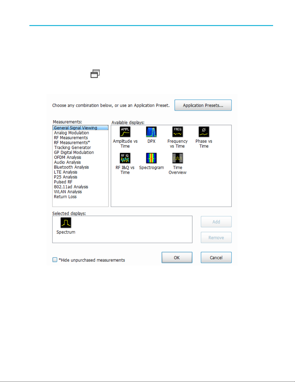
Using the Measurement Displays Selecting Displays

Selecting Displays

Main menu bar: Setup > Displays

Favorites toolbar:

Use the Select displays dialog to choose the displays that appear on the screen.

To select displays:

1. Select Setup > Displays or click the icon.

2. Select one of the choices under Measurements. The measurement chosen determines the c hoices available in Available displays.

3. Double-click the desired display in the Available displays box or select the desired display and click Add.

4. Click OK.

SignalVu-PC Printable Help 41

Using the Measurement Displays Selecting Displays

TIP. See the Features by product (see page 14) topic for more information about which features are available with which connected analyzers.

42 SignalVu-PC Printable Help

Available Measurements Available Measurements

Available Measurements

Available automatic measurements include RF power measurements, OFDM analysis, WLAN analysis, APCO P25 analysis, Bluetooth analysis, LTE analysis, 802.11ad (for ofﬂine analysis only), audio analysis, analog modulation measurements, digital modulation measurements, return loss, distance to fault, and pulsed RF measurements.

See the speciﬁc measurement topic in this document for information about how to take a measurement.

TIP. See the Features by product available

with which connected analyzers.

(see page 14) topic for more information about which features are

Power measurements

Measurem

Channel

Adjacen (ACPR)

Multi-Carrier Power Ratio (MCPR)

Peak/Avg Ratio Ratio of the peak power in the transmitted signal to the average power in the transmitted

CCDF The C

xxx

ent

Power

t Channel Power Ratio

Descript

The tota

Measure

The ratio of the signal power in the reference channel or group of channels to the power in adjacent channels.

signa

time a signal spends at or above a given power level relative to the average power of a measured signal.

ion

l RF power in the selected channel (located in the Chan Pwr and ACPR display).

of the signal power leaking from the main channel into adjacent channels.

l (located in the CCDF display).

omplementary Cumulative Distribution Function (CCDF). CCDF shows how much

SignalVu-PC Printable Help 43

Available Measurements Available Measurements

OFDM analysis

Measurement view Description

Channel Response Plots the channel response (magnitude or phase) versus the subcarrier or frequency.

Here, the channel refers to all sources of signal frequency response impairment up to the analyzer i

nput, including the transmitter itself, as well as any transmission medium

through which the signal travels between the transmitter and the analyzer.

Constellation Shows the WLAN signal modulation amplitude and phase in I (horizontal) versus Q

(vertical) form. For multicarrier WLAN OFDM signals, the points show all data symbol subcarrier

s' modulation. For single-carrier 802.11b, each point corresponds to a single

modulated chip.

EVM

The normalized RMS value of the error vector between the measured signal and the ideal reference signal over the analysis length. The EVM is generally measured on symbol or chip insta

nts and is reported in units of percent and dB. EV M is usually measured after best-ﬁt estimates of the frequency error and a ﬁxed phase offset have been removed. These estimates are made over the analysis length. Displays RMS and Peak values with

of Peak value.

he peak power in the transmitted signal to the average power in the transmitted

Flatness

location

Ratio of t signal

Mag Erro

The RMS magnitude difference between the measured signal and the reference signal magnitude. Displays RMS and Peak values with location of Peak value.

Phase Error

Power

The RMS phase difference between the measured signal and the ideal reference signal.

ys RMS and Peak values with location of Peak value.

Displa

the data symbols' individual subcarrier Power values versus symbol interval (time)

shows and subcarrier (frequency).

xxx

Tracking generator measurement

Measurement Description

Transmission Gain

(Requires Option 04)

xxx

urn loss measurements

Ret

Measure the gain/loss and response of ﬁlters, ampliﬁers, attenuators, and other such devices.

Measurement Description

Cable loss

Measure cable attenuation.

Return loss / VSWR Measure return loss and VSWR on ﬁlters and antennas.

Distance to fault (DTF) Measure distance to fault to ﬁnd the fault.

xxx

44 SignalVu-PC Printable Help

Available Measurements Available Measurements

WLAN measurements

Measurement view Description

Channel Response Plots the channel response (magnitude or phase) versus the subcarr

ier or frequency. Here, the channel refers to all sources of signal frequency response impairment up to the analyzer input, including the transmitter itself, as well as any transmission medium through which the signal travels between the transmitter and the

Constellation Shows the WLAN signal modulation amplitude and phase in I (horizo

analyzer.

ntal) versus Q (vertical) form. For multicarrier WLAN OFDM signals, the points show all data symbol subcarriers' modulation. For single-carrier 802.11b, each point corresponds to a single modulated chip.

EVM

The normalized RMS value of the error vector between the m easure

d signal and the ideal reference signal over the analysis length. The EVM is generally measured on symbol or chip instants and is reported in units of percent and dB. EVM is usually measured after best-ﬁt estimates of the frequency error and a ﬁxed phase offs

et have been removed. These estimates are made over the analysis length. Displays RMS and Peak values with location of Peak value.

Flatness

Ratio of the peak power in the transmitted signal to the average power in the transmitted signal

Mag Error

The RMS magnitude difference between the measured signal

and the reference signal

magnitude. Displays RMS and Peak values with location of Peak value.

Phase Error

The RMS phase difference between the measured signal and the ideal reference signal. Displays RMS and Peak values with location of Peak value.

Power vs Time

The signal power amplitude versus time. For 802.11b signals, the packet Power-On and Power-Down ramp times are also measured.

Summary Shows several measurements of WLAN signal quality.

Symbol Table Shows decoded data values for each data symbol in the a

nalyzed signal packet. For OFDM (non-802.11b) signals, results are presented with subcarrier (frequency) indices in the horizontal dimension and symbol (time) intervals in the vertical dimension. For

802.11b signals, the Preamble, Header, and Data (PSD

U) symbol values are presented

sequentially, with symbol indices in the left column.

xxx

802.11ad measurements

This option is available for ofﬂine analysis only

Measurement view Description

Constellation Shows the 802.11ad signal modulation amplitude and phase in I (horizontal) versus Q

(vertical) form.

EVM vs Time

Shows the EVM plotted against time in seconds or symbols. The analysis region in which the measurement is done is indicated by a purple line in the Time Overview display to indicate the region of analysis.

Symbol Table Shows decoded data values for each data symbol in the analyzed signal packet.

Summary Shows several measurements of 802.11ad signal quality.

xxx

SignalVu-PC Printable Help 45

Available Measurements Available Measurements

Digital Modulation measurements

Measurements for all modulation types except nFSK, C4FM, OQPSK and SOQPSK

Measurement Description

EVM

Phase Error

Mag Error

MER (RMS) The MER is deﬁned as the ratio of I/Q signal power to I/Q noise power; the result is

IQ Origin Offset The magnitude of the DC offset of the signal measured at the symbol times. It indicates

Frequency Error

Gain Imbalance The gain difference between the I and Q channels in the signal generation path.

Quadrature Error The orthogonal error between the I and Q channels. The error shows the phase

Rho

xxx

The normalized RMS value of the error vector between the measured signal and the ideal reference signal over the analysis length. The EVM is generally measured on symbol or chip instants and is reported in units of per cent and dB. EVM is usually measured after best-ﬁt estimates of the frequency error and a ﬁxed phase offset have been removed. These estimates are made over the analysis length. Displays RMS and Peak values with location of Peak value.

The RMS phase difference between the measured signal and the ideal reference signal. Displays RMS and Peak values with location of Peak value.

The RMS magnitude difference between the measured signal and the reference signal magnitude. Displays RMS and Peak values with location of Peak value.

indicated in dB.

the magnitude of the carrier feed-through signal.

The frequency difference between the measured carrier frequency of the signal and the user-selected center frequency of the instrument.

Constellations with gain imbalance show a pattern with a width that is different form height.

difference between I and Q channels away from the ideal 90 degrees expected from the perfect I/Q modulation. Not valid for BPSK modulation type.

The normalized correlated power of the measured signal and the ideal reference signal. Like EVM, Rho is a measure of modulation quality. The value of Rho is less than 1 in all practical cases and is equal to 1 for a perfect signal measured in a perfect receiver.

46 SignalVu-PC Printable Help

Available Measurements Available Measurements

Measurements for OQPSK and SOQPSK modulation types

Measurement Description

EVM

Offset EVM Offset EVM is like EVM except for a difference in the time alignment of the I and Q

Phase Error

Mag Error

MER (RMS) The MER is deﬁned as the ratio of I/Q signal power to I/Q noise power; the result is

in Offset

IQ Orig

ncy Error

Freque

Gain Imbalance The gain difference between the I and Q channels in the signal generation path.

Quadrature Error The orthogonal error between the I and Q channels. The error shows the phase

Rho

xxx

The normalized RMS value of the error vector between the m easured signal and the ideal reference sig

nal over the analysis length. The EVM is generally measured on symbol or chip instants and is reported in units of percent and dB. EVM is usually measured after best-ﬁt estimates of the frequency error and a ﬁxed phase offset have been removed. These estima

tes are made over the analysis length. Displays RMS and Peak values with

location of Peak value.

samples. For EVM, I and Q samples are collected at the same time, for every symbol decision po

int (twice the symbol rate for offset modulations). For Offset EVM, the I and Q symbol decision points are time-aligned before collecting the I and Q samples. In this case, one I and one Q sample is collected for each symbol (half as many samples as the same numbe

The RMS pha

r of symbols for (non-offset) EVM.

se difference between the measured signal and the ideal reference signal.

Displays RMS and Peak values with location of Peak value.

The RMS magnitude difference between the measured signal and the reference signal magnitude. Displays RMS and Peak values with location of Peak value.

ed in dB.

indicat

The mag

nitude of the DC offset of the signal measured at the symbol times. It indicates

the magnitude of the carrier feed-through signal.

The frequency difference between the measured carrier frequency of the signal and the user-selected center frequency of the instrument.

ellations with gain imbalance show a pattern with a width that is different form

Const height.

difference between I and Q channels away from the ideal 90 degrees expected from the

fect I/Q modulation. Not valid for BPSK modulation type.

per

normalized correlated power of the measured signal and the ideal reference signal.

The Like EVM, Rho is a measure of modulation quality. The value of Rho is less than 1 in all practical cases and is equal to 1 for a perfect signal measured in a perfect receiver.

SignalVu-PC Printable Help 47

Available Measurements Available Measurements

Measurements for nFSK modulation types

Measurement Description

Peak FSK err Peak value of the frequency deviation error at the symbol point.

RMS FSK Err RMS value of the frequency deviation error at the symbol point.

Peak Mag Err

The Peak magnitude difference between the measured signal and the reference signal magnitude.

RMS Mag Err The RMS magn

itude difference between the measured signal and the reference signal

magnitude.

Freq Error

The frequency difference between the measured carrier frequency of the signal and the user-selected center frequency of the instrument.

Freq Deviation

Frequency distance from the center frequency at the symbol point.

Symbol Rate Error This compares the user-entered symbol rate to the instrument calculated symbol rate of

yzed signal.

the anal

Symbol R

ate

When in A

uto-symbol rate, the instrument calculates the symbol rate of the signal and the instrument calculates the error between the user entered value and the instrument calculated value.

xxx

Measurements for C4FM modulation type

Measurement Description

RMS Error Magnitude RMS value of the frequency deviation error at the symbol point.

Carrier Frequency Error Frequency difference between averaged signal frequency and the center frequency.

Deviation

Length

xxx

Frequency distance from the center frequency at the symbol point.

Number of symbols in the analysis area.

Analog Modulation measurements

asurements for AM modulation

asurement

+AM Positive peak A M value.

-AM Negative peak AM value.

otal AM

xxx

Measurements for FM modulation

Measurement Description

+Pk

–Pk

RMS RMS value of the frequency deviation.

Pk-Pk/2 Peak-to-peak frequency deviation divided by 2.

Pk-Pk

xxx

scription

otal AM value, which is equal to the peak-peak AM value divided by 2.

Positive peak frequency deviation.

Negative peak frequency deviation.

Peak-to-peak frequency deviation.

48 SignalVu-PC Printable Help

Available Measurements Available Measurements

Measurements for PM modulation

Measurement Description

+Pk Positive peak phase deviation.

–Pk Negative peak

RMS RMS value of t

phase deviation.

he phase deviation.

Pk-Pk Peak-to-peak phase deviation.

xxx

APCO P25 measurements

Measurement Description

RF output power

Measure of RF output power when the transmitter is connected to the standard load during deﬁned duty cycle.

Operating frequency accuracy Measure of the ability of the transmitter to operate on its assigned frequency.

Unwanted emissions (ACPR) Ratio of the total power of a transmitter under prescribed conditions and modulation to

that of the output power that falls within a prescribed bandwidth centered on the nominal frequency of adjacent channels.

Frequency deviation

Measurement of the amount of frequency deviation that results for a Low Deviation and High Deviation test pattern.

Modulation ﬁdelity Measures the degree of closeness to which the modulation follows the ideal theoretical

modulation determined by the rms difference between the actual deviation and the expected deviation for the transmitted symbols.

Symbol rate accuracy Measures the ability of the transmitter to operate at the assigned symbol rate (4.8 kHz

for Phase 1, 6 kHz for Phase 2).

Transmitter power and encoder attack time

Measures the time required for a transmitter to prepare and transmit information on the radio channel after changing state from standby to transmit (applies to conventional mode).

Transmitter power and encoder attack time with

Measures the time required for a transmitter to prepare and transmit information on the radio channel after the receiving channel changes state from busy to idle.

busy/idle operations

Transmitter throughput delay

Measures the time it requires for audio changes in the microphone to be encoded and transmitted over the air.

Transient frequency behavior Measures the difference of the actual transmitter frequency and assigned transmitter

frequency as a function of time when the RF output power is switched on or off.

HCPM transmitter logical channel time alignment

Measures the ratio of total transmitter power under prescribed conditions and modulation to the peak power that falls in a prescribed bandwidth centered on the nominal frequency of the adjacent channel during the transmitter power ramping interval.

xxx

Bluetooth measurements

Measurement Description

Modulation characteristics

Veriﬁes that the modulation characteristics of the transmitted signal are correct. This measurement can only be done if the payload has the bit pattern 10101010 or 11110000.

Carrier frequency offset and drift

Veriﬁes that the carrier frequency offset and carrier drift of the transmitted signal is within the speciﬁed limits for the Basic Rate and Low Energy standards. This test can be done only if the payload contains 10101010 bit pattern.

SignalVu-PC Printable Help 49

Available Measurements Available Measurements

Measurement Description

Output power Veriﬁes the maximum peak and average power emitted from the EUT. The standard

is test be done for a PRBS payload pattern.

he in-band spectral emission is within limits. The standard document

In-band emiss

ion / ACPR

recommends th

Veriﬁes that t recommends that this measurement be done with Hopping off, ﬁnding the integrated power in 1 MHz band (with RBW 100 kHz) in 80 channels starting from 2401 MHz to 2481 MHz. The inte

grated power values calculated in the adjacent channels are compared against recommended limits (except the three channels around transmitted frequency). This measurement is referred to as ACPR in the Basic Rate standards document.

20 dB bandwidth

Veriﬁes if the emissions inside the operating frequency r ange are within limits. This measuremen

t is done with Hopping off. The difference between frequency points at which the power level drops to 20 dB below the peak power of the emission is found as 20 dB bandwidth.

Frequency range

Power density

band spurious emission

Out-of-

Relative power

These measurements verify if the emissions inside the operating frequency range are within th

This meas

This mea

Veriﬁes

e limits.

urement veriﬁes the maximum RF output power density.

surement can be done for FCC or ETSI masks using the Spurious display.

the relative power in the GFSK and PSK part of the Enhanced Data Rate signal.

This measurement is supported only when an Enhanced Data Rate signal is detected.

xxx

LTE measurements

Measurement Description

Cell ID detection The Cell ID is detected from the input LTE signal.

For TDD and FDD.

Adjacent Channel Leakage Ratio (ACLR)

The Adjacent Channel integrated power is calculated and shown. The relative power compared to the reference signal is also computed. The computed power is compared against limits suggested by the selected standard and pass/fail is reported.

For TDD and FDD.

Channel Power

The channel power is calculated in the channel bandwidth.

For TDD and FDD.

Occupied Bandwidth The Occupied bandwidth is calculated as bandwidth containing 99% of the total

integrated power in the selected span around the selected center frequency.

For TDD and FDD.

Operating Band Unwanted Emission

The power in the offset regions is calculated and presented and compared against limits set in the offset and limits table and pass/fail is reported.

For TDD and FDD.

OFF

The power in off-slot region is computed and compared against selected limits.

For TDD only.

xxx

Pulse measurements

Measurement Description

Average ON Power

Peak Power Maximum power during pulse on.

The average power transmitted during pulse on.

50 SignalVu-PC Printable Help

Available Measurements Available Measurements

Measurement Description

Average Transmitted Power The average power transmitted, including both the time the pulse is on and the time

it is off, and all transition times.

Pulse Width

Rise Time

Fall Time

Repetition Interval

Repetition Rate

Duty Factor (%) The ratio of the width to the pulse period, expressed as a percentage.

Duty Factor (Ratio) The ratio of the pulse width to the pulse period.

Ripple Ripple is the peak-to-peak ripple on the pulse top. It does not include any preshoot,

Ripple dB The Ripple measurement expressed in dB.

Droop

pdB

Droo

rshoot

Ove

Overshoot dB The Overshoot measurement expressed in dB.

Pulse-ref-Phase Difference The phase difference between the current pulse and the ﬁrst pulse in the analysis

ulse-ref Freq Difference

RMS Freq Error The RMS Frequency Error measurement is the RMS average of the Freq Error vs. Time

Max Freq Error

RMS Phase Error The RMS Phase Error measurement is the RMS average of the Phase vs Time trace,

The time from the rising edge to the falling edge at the –3 dB / –6 dB level (50%) of the user selected

Thetimerequ selected 100% level.

The time required for a signal to fall from 90% to 10% (or 80% to 20%) of the user selected 100% level.

The time from a pulse rising edge to the next pulse rising edge.

The inverse of repetition interval.

overshoot, or undershoot. By default, the ﬁrst 25% and the last 25% of the pulse top is exclude the pulse.

If the Amplitude units selected in the Amplitude panel (affects all amplitude measurements for the results will be in %Watts. T he default for the general Units control is dBm, so the Ripple results default is %Watts.

See al

Droop is the power difference between the beginning and the end of the pulse On time. A

ight-line best ﬁt is used to represent the top of the pulse. The result is a percentage

stra referenced to the Average ON Power.

The D

amount by which the signal exceeds the 100% level on the pulse rising edge. Units

The are %Watts or %Volts.

window. The instantaneous phase is measured at a user-adjustable time following the

sing edge of each pulse.

he difference between the frequency of the current pulse and frequency of the previous

T pulse. The instantaneous frequency is measured at a user-adjustable time following the rising edge of each pulse.

trace, computed over the Measurement Time.

The maximum frequency error is the difference between the measured carrier frequency of the signal and the user-selected center frequency of the analyzer.

computed over the Measurement Time.

100% level. Level is user selectable for Volts or Watts.

ired for a signal to rise from 10% to 90% (or 20% to 80%) of the user

d from this measurement to eliminate distortions caused by these portions of

analyzer) are linear, the Ripple results will be in %Volts. For log units, the Ripple

so Ripple

roop measurement expressed in dB.

(see page 886).

SignalVu-PC Printable Help 51

Available Measurements Available Measurements

Measurement Description

Max Phase Error

Freq Deviati

Phase Deviation

Impulse Response Amplitude

Impulse Response Time

Absolute Frequency

Pulse-Pulse Frequency Difference

Pulse-Pulse Phase Difference The phase difference between the selected pulse and the ﬁrst pulse in the analysis

xxx

The phase is measured at each point during the pulse's ON time. The phase error for each point is t

he difference between the measured phase value and the calculated ideal phase value. After the phase error is calculated for all points in the acquisition record, the largest error in the positive direction and the largest in the negative direction are determined. W

hichever of these two values has the greater absolute value is designated

the Max Phase Error.

The Frequency Deviation measurement is the difference between the maximum and minimum measured values of the signal frequency during the Measurement Time.

The Phase Deviation is the difference between the maximum and minimum Phase values measured du

The differ

The diffe

The absol

ring the ON time of a pulse.

ence in dB between the levels of the main lobe and highest side lobe.

rence in time between the main lobe and highest side lobe.

ute pulse frequency m easured at a point speciﬁed by the user. The measurement includes carrier frequency as well. The measurement point should be within the pulse width, starting from the 50% point.

The difference between the frequency of the current pulse and frequency of the previous

he instantaneous frequency is measured at a user-adjustable time following the

pulse. T rising edge of each pulse.

window. T he instantaneous phase is measured at a user-adjustable time following the

g edge of each pulse.

risin

52 SignalVu-PC Printable Help

General Signal Viewing Overview

Overview

The displays in General Signal Viewing (Displays > Measurements > General Signal Viewing) are:

Amplitude vs Time

DPX Spectrum

Frequency vs Time

Phase vs Tim

RF I & Q vs Time

Spectrogram

Spectrum

Time Overview

These displays p rovide extensive time-correlated multi-domain views that connect problems in time, frequency, phase and amplitude for enabling you to more quickly understand cause and effect when troubleshooting.

TIP. See the Features by product available with which connected analyzers.

DPX primer

The information in this section is from the Tektronix DPX Primer, available separately as an application note and for download from www.tek.com. The DPX display can detect extremely brief signals and processes many thousands of spectrums per second. It then displays all these spectrums as a color-graded bitmap that reveals low-amplitude signals beneath stronger signals sharing the same frequency at different times.

(see page 14) topic for more information about which features are

The strong signal in the DPX spectrum graph, showninFigure1,isarepeatingpulseataﬁxed frequency. There is also a lower-power CW signal that steps very quickly through the same span. During the pulse's

n time, the power of the two signals is additive, resulting in nearly undetectable differences in the pulse

o envelope shape. But during the time the pulse is off, the sweeping signal is detected and shown in its true form. Both signals are visible in the bitmap because at least one full cycle of their activities occurs within a single DPX display update.

SignalVu-PC Printable Help 53

General Signal Viewing DPX primer

Figure 1

Compare the display of a traditional swept spectrum analyzer (Figure 2) and that of a real-time signal analyzer with a DPX display (Figure 3). The signal captured is a typical WLAN interchange between a nearby PC and a more-distant network access point (AP). The laptop signal is nearly 30 dB stronger than the AP's signal because it is closer to the measuring antenna.

Figure 2

Figure 3

The traditional swept spectrum analyzer display, Figure 2, uses line traces that can show only one l evel for each frequency point, representing the largest, the smallest or the average power. After many sweeps, the

54 SignalVu-PC Printable Help

General Signal Viewing DPX primer

Max Hold trace shows a rough envelope of the stronger laptop signal. +Peak detection was selected for the other trace in an atte mpt to capture the weaker but more frequent AP signal, but the bursts are very brief, so the likelih capture the entire spectrum of a bursted signal due to the architecture of the swept spectrum analysis.

ood of seeing one in any particular sweep is small. It will also take a long time to statistically

The DPX displ instead of a line trace, you can distinguish many different signals occurring within each update period and/or different version of the same signal varying over time. The heavy band running straight across the lower third of the graph is the noise background when neither the laptop nor the AP is transmitting. The red lump of energy in the middle is the ON shape of the AP signal. Finally, the more delicate spectrum above the others is the laptop transmissions. In the color scheme used for this demonstration (“Temperature”), the hot red laptop signal, in yellow, green and blue, has higher amplitude but doesn't occur nearly as often as the AP transmissions because the laptop was downloading a ﬁle when this screen capture was taken.

ay, Figure 3, reveals much more insight on the same signal. Since it is a bitmap image

color indicates a signal that is much more frequent than signals shown in cooler colors. The

How DPX works

This section explains how DPX displays are created. The input RF signal is conditioned and down-converted as usual for a signal analyzer, then digitized. The digitized data is processed in SignalVu-PC, creating very fast spectral transforms. The resulting frequency-domain waveforms are

rized to create the bitmaps.

raste

The DPX bitmap that you see on screen is composed of pixels representing x, y, and z values for frequency,

itude, and Density. A multi-stage process, shown in the following four ﬁgures, creates this bitmap,

ampl starting with analog-to-digital conversion of the input signal.

Simpliﬁed Flow of Multi-stage Processing from RF Input Through to Spectrum Processing:

Figure 4a. RF signals are downconverted and sampled into a continuous data stream.

Figure 4b. Samples are segmented into data records for FFT processing based on the selected resolution bandwidth.

Figure 4c. Data records are processed in the DPX transform engine

SignalVu-PC Printable Help 55

General Signal Viewing DPX primer

Figure 4d. Overlapping the FFTs shortens the minimum event duration required for 100% probability of intercept.

Collecting spectral data. Sampling and digitization is continuous. The digitized data stream is chopped

into data records whose length is based on the desired res requirement is placed on FFT length by the desired number of points in a trace. The DPX transform engine performs a discrete Fourier transform on each record, continually producing spectral waveforms.

As long as spectral transforms are performed faster than the acquisition data records arrive, the transforms can overlap each other in time, so no events are missed in between. Minimum event length for guaranteed capture depends on the length of the data records being transformed. An event must last through two consecutive data records in order for its amplitude to be accurately measured. Shorter events are detected and visible on screen, but may be attenuated. The DPX Spectrum RBW setting determines the data record length; narrow RBW ﬁlters have a longer time constant than wide RBW ﬁlters. Thi requires longer FFTs, reducing the transform rate.

olution bandwidth (RBW). An additional

s longer time constant

The spectral waveforms are plotted onto a grid of counting cells called the “bitmap database”. The num held by each database cell is the z-axis count. For simplicity, the small example grid used in the following grids is 11x10, so our spectral waveforms will each contain 11 points. A waveform contains one (y) amplitude value for each (x) frequency. As waveforms are plotted to the grid, the cells increment their values each time they receive a waveform point.

Figure 5. Example 3-D Bitmap Database after 1 (left) and 9 (right) updates. Note that each column contains the same total number of “hits”.

The grid on the left shows what the database cells might contain after a single spectrum is plotted into it. Blank cells contain the value zero, meaning that no points from a spectrum have fallen into them yet.

The grid on the right shows values that our simpliﬁed database might contain after an additional eight spectral transforms have been performed and their results stored in the cells. O ne of the nine s pectrums happened to be computed as a time during which the signal was absent, as you can see by the string of “1” occurrence counts at the noise ﬂoor.

ber

Frame updates. The maximum rate for performing the variable-length frequency transforms that produce

those waveforms varies with the PC you use and the length of the transform. Rates greater than 1 million transforms per second are performed with the RSA7100A. Measurement settings that slow this transform

56 SignalVu-PC Printable Help

General Signal Viewing DPX primer

rate include narrowing the RBW and increasing the number of points for the line traces available in the DPX display along with the bitmap. Even at their slowest, spectral transforms are performed orders of magnitude fas

ter than a physical display can respond, and also too fast for humans to see, so there's no need to update the screen or measurements at this rate. Instead, the grid collects thousands of waveforms into “frames”, each covering about 50 milliseconds (ms). The actual frame rate varies with resolution bandwidth and the processor used in your PC. After each frame's waveforms have been mapped into the grid, the cell occurrence counts are converted to colors and written to the DPX bitmap, resulting in a bitmap update rate of around 20 per second.

Frame length sets the time resolution for DPX measurements. If the bitmap shows that a -10 dBm signal at 72.3 MHz was present for 10% of one frame's duration (5 ms out of 50 ms), it isn't possible to determine

just from the DPX display whether the actual signal contained a single 5 ms pulse, one hundred

50 microsecond (μs) pulses, or something in between. For this information, you need to examine the spectral details of the signal or use another display with ﬁner time resolution, such as Frequency vs. Time or Amplitude vs. Time.

Converting occurrence counts to color. About 20 times per second, the grid values are transferred to the

next pr

ocess step, in which the z-axis values are mapped to pixel colors in the v isible bitmap, turning data into information. In this example, warmer colors (red, orange, yellow) indicate more occurrences. The color palette is user-selectable, but for now we will assume the default “temperature” palette.

Number of Occurrences Color

0black

1blue

2 light blue

4 green blue

6yellow

8 red orange

9red

xxx

cya

green

orange

The result of coloring the database cells according to the number of times they were written into by the nine spectrums, one per pixel on the screen, creates the DPX displays.

SignalVu-PC Printable Help 57

General Signal Viewing DPX primer

Figure 7. Color-coded low-resolution example (left) and a real DPX display (right).

In addition to the choice of palette, there are z-axis scaling adjustments for Maximum, Minimum, and Curve. Maximum sets the occurrence value that will be mapped to the highest color in the palette. Minimum sets the occurrence value for the lowest color. In the “temperature” palette, the highest color is deep red and the lowest i s dark blue. Occ urrence values less than the selected Minimum are represented with black pixels, while pixels that exceed the selected Maximum are red in hue but somewhat transparent. Values between Maximum and Minimum are represented by the other colors of the palette.

Adjusting the Minimum above the black default allows you to concentrate most of your color resolution over a small range of medium or higher occurrence rates to visually discriminate between different signals that have nearly equal probability values.

To see why adjustable color scaling is useful compare the following ﬁgures. On the Scale tab, the Max control is set to 100% in the ﬁrst ﬁgure. The range of colors now covers the full z-axis range of densities from 0 to 100%. The signals used to create this bitmap are fairly diffused in both frequency and amplitude, so most pixels have low occurrence counts or dens palette is unused.

Figure 8. DPX spectrum bitmap with default color scale settings.

When the Auto Color button is selected, the Maximum control's value is set to the highest pixel value in the current bitmap, shown below. Now none of the available colors remain unused. The entire palette is mapped to the occurrence values present at the time the button is selected, providing better visual

ity values and the upper half of the color

58 SignalVu-PC Printable Help

General Signal Viewing DPX primer

resolution for low densities. Selecting the Autoscale button in the DPX display scales all three axes based on current results.

Figure 9. The Auto Color function optimizes the color scale settings.

Color mapping curves

The mappi choose the shape of the mapping equation. A Curve setting of 1 selects the straight-line relationship. Higher Curve numbers pull the curve upwards and to the left, concentrating color resolution on lower densities. Settings less than 1 invert the curve, moving the focus of the color range towards higher density values. The following ﬁgure shows the mapping curves.

gure 10. Representative color mapping curves for the “Temperature” palette.

ng between z-axis values and color does not have to be linear. The Curve control lets you

ing the same signal shown in Figures 8 and 9, the impact of the Curve control can be observed. With

Us the Curve control set to 1 in the Scale tab, shown in Figure 11, the mapping between color and density is linear, so the colors spread evenly across the full density range. The color distribution is visible in the colored palette illustration to the left of the Curve control in the Settings panel.

SignalVu-PC Printable Help 59

General Signal Viewing DPX primer

Figure 11. Ov

When the Cur the density range, and only the dark blues are assigned to densities below 50%. Note the difference in the palette illustration.

Figure 12. Adjusting to values less than 1, increases the contrast for viewing events in the top half of the selected density range.

In Figure 13, the Curve control is increased to 3. The majority of colors shifts to the lower half of the density scale, but various shades of orange and red are still available for densities above 50%.

er a narrow Signal Density range, the color curve is set to 1.

ve control is set to 0.5, as shown in Figure 12, the best color resolution is in the upper half of

Figure 13. For color curve settings greater than 1, better contrast is provided for events near the low end of the density range.

Swept DPX

DPX Spectrum is not limited in span by its real-time bandwidth. Like the regular Spectrum display, DPX Spectrum steps through multiple real-time frequency segments, building a wide-span display with line traces and the bitmap. See Figure 14.

60 SignalVu-PC Printable Help

General Signal Viewing DPX primer

Figure 14. Off-air ambient signals over a 1 GHz span in the swept DPX display.

The analyzer “dwells” in e ach frequency segment for one or more DPX frames, each containing the results of up to 14, sweep for up to 100 seconds before moving to the next step. While dwelling in a segment, the probability of intercept for signals within that frequency band is the same as in normal, real-time spans.

A full pixel bitmap is created for every segment and compressed horizontally to the number of columns needed for displaying the frequency segment. Compression is done by averaging pixel densities of the points being combined together. The ﬁnal swept bitmap contains a representation of the same pixel bitmap resolution, just like the non-swept bitmaps. Line traces are also created in full for each segment, and then horizontally compressed to the user-selected number of trace points for the full span.

600 spec tral transforms. Dwell time is adjustable, so you can monitor each segment of the

A complex algorithm for determining the number and width of each frequency segment has been implemented. The variables in the equation include user-adjustable control settings like Span, RBW, and

r of trace points, RF and IF optimization, and Acquisition BW. Installed hardware options also can

numbe affect the span segmentation.

pful piece of information for operators is the actual Acquisition Bandwidth used for capturing each

Ahel segment. “Acq BW” is shown in the Acquire control panel on the Sampling Parameters tab. Acq BW is typically set automatically by the instrument, basedontheneedsofalltheopendisplays,butcanalsobe set manually. In either case, the displayed bandwidth is used for every frequency se gment in the swept DPX d isplay, though in practice, the displayed portion of the segment is somewhat narrower than the actual Acquisition BW, for performance reasons.

The entire instrument frequency range of many GHz can be covered in a DPX sweep. The Dwell Time control sets the amount of time DPX spends in each segment. This control, shown b elow, can be set

etween 50 ms and 100 seconds.

Figure 15. During swept DPX operation, the Dwell time control adjusts the observation time of each frequency segment used to construct the composite DPX display.

SignalVu-PC Printable Help 61

General Signal Viewing DPX primer

Guaranteed capture in DPX real-time spans

All Tektronix real time spectrum analyzers are speciﬁed for the minimum signal duration for 100% probability of capture and display. This number can vary based on the processor used for SignalVu-PC. In the case of the RSA7100A, the processor is from Tektronix, and we provide published performance in the datasheet an download from www.tek.com). In the case of USB RF spectrum analyzers, minimum signal duration can be as brief as 16 μs. See the datasheet for your instrument to determine its performance.

You can also, at any time, have the instrument report its minimum signal duration by displaying it on the DPX spectrum screen as follows.

1. Check that the DPX spectrum display is active.

d RSA7100A Speciﬁcations and Performance Veriﬁcation Technical Reference (available for

2. Click

3. Select the Prefs tab.

4. Check th

on the right side of the display.

The fol under various combinations of Span and RBW in DPX for a representative signal analyzer. As you can see, MSD is affected by multiple factors.

To demonstrate the POI in action, a challenging bi-stable signal is used. A CW sinusoid sits at 2.4453 GHz most of the time, but every 1.28 seconds, its frequency changes for about 100 μs before returning to normal. The duty factor of this transient is less than 0.01%.

Figure 16 shows a swept analyzer set up for a 5-second sweep of its MaxHold trace. It shows that there is something occurring around the signal. This sweep rate was empirically dete rmined to be the optimum rate for reliable capture of this signal in the shortest time. Faster sweep times can reduce the probability of intercept and result in fewer intersections of the sweep with the signal transient.

lowing table shows the speciﬁed minimum signal duration (MSD) for 100% probability of intercept

to view the DPX settings control panel.

e Show parameter readouts box. The minimum signal duration for 100 % POI will appear

62 SignalVu-PC Printable Help

General Signal Viewing DPX primer

Figure 16. Swept spectrum display of the infrequent transient.

The DPX display shown in F lot more information can be discovered about the transient. It is obvious at ﬁrstglancethatthesignalis hopping by about 3 MHz, with 1.2 MHz of frequency overshoot on transitions

Figure 17. The DPX spectrum display after 5 seconds. The MaxHold trace is cyan.

igure 17 shows the exact same event, also captured over a 5 second period. A

Guaranteed capture in DPX swept spans

Probability of intercept (POI) for signals within a single segment, while DPX is dwelling in that segment, is the same as for non-swept DPX operation. But just as in traditional swept analyzers, during the time the acquisition is tuned to any one segment, the a nalyzer is not monitoring signals in any of the other segments, so probability of capture in segments other than the current one is zero. Because of the wide real-time

SignalVu-PC Printable Help 63

General Signal Viewing DPX primer

bandwidth, the number of segments n eeded to cover the span is much less than for swept analyzers, so the overall probability of intercept is signiﬁcantly better for DPX sweeps.

Another factor affecting POI is number of trace points. The bitmap is always 801 points wide, but the line traces allow user selection for number of points. 801 is the default and the other choices are 2401, 4001, and 104 lower waveform update rate increases the minimum signal duration proportionally. This caution a pplies for swept and non-swept operation. The trace length control is on the Prefs tab in the DPX control panel.

01. Frequency transforms for traces containing more than 801 points take longer, and this

DPX Density measurements

NOTE. DPX Density measurements are only available when an RSA7100A is connected.

Density is a measure of the amount of time during a deﬁned measurement period during which signals are present within a particular area of the DPX Spectrum bitmap. A clean CW tone gives a 100% reading, while a p how density is computed from hit counts.

ulse that is on for one microsecond out of every millisecond reads 0.1%. This section describes

If we pl we already plotted), each column ends with a total of 50 hits (Figure 18). The density for any one cell in a column is its own count value divided by 50, expressed in percent as shown in Figure 19. The math is very simple: a cell with 24 counts has a 48% density. In practice, instead of batches of 50 waveforms, we collect a frame of thousands of waveforms before each update to the density bitmap.

Figure 18. Grid showing cell counts after 50 waveforms. For each column, the sum of z-axis values is 50.

ot 41 more waveforms into the example grid we used previously in Figure 6 (in addition to the nine

64 SignalVu-PC Printable Help

General Signal Viewing DPX primer

Figure 19. Grid after converting occurrence counts to percent density values. The sums of the cell density measurements within each column are all 100%.

Measuri

Hit counts are cleared after every frame update, as long as Persistence is not turned on. The density value fo Markers can be used to see the Density value for one or more individual points on the screen, enabling measurements of the signal density at any interesting point in the DPX display.

In Figure 20, Wireless LAN signals are analyzed in the presence of a Bluetooth radio signal in the 2.4 GHz ISM band.

Figure 20. DPX display of WLAN and Bluetooth signals, with a marker on the highest signal.

ng density with markers

r any pixel is simply the percent of time it was occupied during the most recent 50 ms frame.

The “Marker to Peak” function was used to ﬁnd the peak signal recorded in the display. The marker readout in the upper left corner of Figure 20 shows the Density, Amplitude, and Frequency for the pixel you selected with the marker. By adding additional markers, you can measure the signal density differences between multiple signals of interest.

SignalVu-PC Printable Help 65

General Signal Viewing DPX primer

Marker peak search in the DPX bitmap

Markers on the DPX bitmap can search for peaks, similar to marker pea k sea rching on spectrum line traces. For a human, it is pretty easy to discern “signals” in the bitmap picture. Your brain intuitively identiﬁes strings of contiguous bright pixels. This isn't so easy for a computer. The ﬁrst thing the RSA must do for an through these density peaks for the amplitude peaks you want to ﬁnd.

ypeaksearchisanalyzepixeldensityvaluesto identify apparent signals. Then it can sift

Z-axis dens

ity values for the pixels in each column of the bitmap are internally converted into histograms to ﬁnd density peaks indicating the presence of signals. Table 2 shows the ﬁve middle columns from the example grid we used to illustrate density measurements in a previous section (Figure 19). The density values for each pixel in the middle, highlighted column are plotted on the y axis in the bar chart in Figure 21. The bar chart x axis is bitmap row number, numbering from the top of the table.

Table 1: Bitmap section showing density values.

0% 0% 0% 0% 0%

0% 0% 8% 0% 0%

0% 0% 12% 0% 0%

0% 0% 26% 0% 0%

0% 0% 36% 0% 0%

0% 2% 6% 2% 0%

4% 8% 0% 8% 0%

86% 82% 4% 76% 12%

10% 8% 6% 14% 86%

0% 0% 2% 0% 2%

xxx

Figure 21. Bar chart of the density values in the bolded column of Table 2.

Assume that Density Threshold is set to 5% and Density Excursion to 5% also. Starting with x=1 in the bar chart, test each bar against the threshold. The threshold criteria is met at x=2. Keep testing until you

66 SignalVu-PC Printable Help

General Signal Viewing DPX primer

ﬁnd a bar that is shorter than the previous bar by at least the Excursion setting. In this case it is x=6. This tells us that a “signal” covers rows 2 through 5. Its density peak is at row 5.

Now you can look for another peak. Continue looking at bars to the right and you will ﬁnd a density value at row 9 that meets the threshold criteria, but since there are no bars to the right of it that meet the excursion cr had 1% density, then row 9 would be a density peak.

iteria, we can't declare row 9 a signal because it fails to meet the excursion criteria. If row 1

Once densit When the Peak button is selected, the analyzer checks the histograms of every column in the bitmap and ﬁnds the density peak with the highest amplitude. The amplitude search has its own versions of Threshold and Excursion settings, but in dBm and dB units. When Next Peak Down command is given, the search will scan inside the current column for the next density peak. Next Peak Right examines each column to the right of the current marker location to locate density peaks that also meet the amplitude peak criteria.

To demonstrate the value of marker peak search in the DPX bitmap, we will use the time-multiplexed signals showing multiple amplitude levels from an example earlier in this manual. The Peak button and its m density peak of highest amplitude in the bitmap.

Figure 22. The marker was positioned by selecting the Peak button. Density, frequency, and amplitude measurements at the marker are displayed in the upper left corner of the graph.

y peaks are found for all columns in the bitmap, we can start looking for the amplitude peaks.

enu equivalent place the active marker on the peak signal in Figure 22. The peak signal is the

The Marker Toolbar, at the bottom of Figure 22, allows easy navigation of peak signals (Peak Left, Peak Right, Next Peak Up,orNext Peak Down). Selecting the arrow keys enables the marker to search for amplitude/density peaks at other frequencies, while the Next Peak Up and Next Peak Down arrows

nable the marker to search for other high-density points at the same frequency.

In the Deﬁne Peaks tab of the Deﬁne Markers c ontrol panel, Figure 24, you can adjust the density threshold

nd excursion controls to modify search behavior. The amplitude threshold and excursion controls also

a apply to DPX marker searches. Smoothing keeps the marker from ﬁnding multiple peaks within the same apparent signal by averaging an adjustable number of pixel densities together, but it does not affect the single-pixel measurement readout displayed by the marker.

SignalVu-PC Printable Help 67

General Signal Viewing DPX primer

Figure 24. Amplitude and Signal Density controls can be adjusted to deﬁne Peak search behavior.

Density measurements over an adjustable area (The Box)

The density for a single pixel is its ratio of actual hits versus possible hits over a deﬁned time period, and markers display these density values. For measuring density over an area larger than one pixel, the DPX display i

If you could make the box so narrow that it contained only points within a single column of pixels, the density three pixels tall and the density values for these pixels were 4, 2, and 7% respectively, the overall density for the three-pixel area would be 13%. Imagine a box one pixel wide and as tall as the graph. Assume that the input signal's amplitude was such that all hits fell at or near the vertical center of the screen. Since 100% of the waveforms written to the bitmap passed through the box, the density for the box is 100%.

ncludes a measurement box you can resize and drag around in the DPX display.

of this area would be the sum of the included pixels' density values. For example, if the box was

When you widen the box to cover a broader range of frequencies, software computes the d ensity sum for the included pixels in each column inside the box. The aggregate density value for this box is the average density, calculated by adding the column density sums then dividing by the number of columns. For a 100%

ult, there must not be any hits above the top edge of the box or below its bottom edge. In other words,

res every waveform drawn across the graph entered the box through its left side and exited the box through its right side, with no excursions out the top or bottom. Figure 24 demonstrates this principle on a CW signal. As you can see on the left-hand side, no amplitudes exist above or below the box; the density of the signal is 100%. On the right hand side, there are signals below the box, therefore the density is less than 100%.

68 SignalVu-PC Printable Help

General Signal Viewing DPX primer

Figure 24. Density of signals deﬁned within an area. Left: Correct measurement of a CW signal. All columns in the box include the signal. Right: Incorrect measurement area. The measurement is accurate, but probably not what you expected.

Some columns in the box contain no hits, so they contribute zeros to the calculation of average density.

The densi units you have selected for measurements. The box is not draggable when the selected units are linear (such as Amps, Volts, Watts…), though you can still ad just its size and location using the Frequency and Amplitude controls. Since the vertical scale is non-linear, a box of constant amplitude changes visual height as it changes vertical position, a disconcerting e ffect if you are trying to drag it.

Figure 25. DPX Density control panel is used to deﬁne the area of interest for DPX density measurements.

A readout will appear somewhere in the graph. If the box is off-screen, the readout will be accompanied by an arrow pointing towards the invisible box. Drag the density readout to the area you want to measure.

ty measurement box’s vertical size and location are always set in dB and dBm, no matter what

Persistence

Previous sections of this topic have assumed that persistence was not applied to the DPX bitmap. Without persistence, hit counts in the grid are cleared after eac h frame update. Now we will describe how persistence modiﬁes this behavior, starting with inﬁnite persistence because it is simpler than variable persistence.

Hit counts are not cleared between frames if inﬁnite persistence is enabled. When the instrument is set up for continuous acquisitions, hits keep collecting until you stop acquisitions or click the Clear button above the DPX display. Software keeps track of the total number of waveforms computed during the entire collection period. Density equals the total number of hits to a cell divided by the total number of waveforms.

SignalVu-PC Printable Help 69

General Signal Viewing DPX primer

Variable persistence is trickier. A single-occurrence signal shown in the bitmap does not disappear suddenly upon the next frame update, nor does it linger forever. It fades gradually aw ay. The user sets atimeconstan Fading is accomplished by reducing the hit count in every cell, after each frame update, by a factor based on the persistence time constant. The longer the time constant, the less the hit counts are reduced.

Figure 26. Example of fast transient discovery with and without variable persistence turned on. In the display on the left, with variable persistence of 10 seconds, the occasional sub-second transient that spikes up above the normal signals is held in the display rather than disappearing as soon as the signal goes away. The display on the right, with persistence turned off, requires watching the display continually to see the brief signal.

t for the Dot Persistence control which determines how long it takes for signals to fade.

Not only are single-occurrence signals allowed to remain in the display for awhile by variable persistence, additional hits keep piling on. The result is that cell values are no longer pure hit counts; they include counts due to new hits from waveforms plus proportionally reduced counts from prior frames. As part of translating hit counts into density values, a new software algorit discriminate between the effects of persistence and the arrival of new hits. The inﬂationary effects of persistence on cell counts are removed, so density readings represent the true ratio of actual hits to possible hits over the persistence interval.

The density computation for variable persistence is a very good estimate of true signal density, with errors of less than 0.01%. For exact density measurements, use either no persistence or inﬁnite persistence.

Another subtlety of persistence is its smoothing effect on the density measurement of intermittent signals. Consider a pulse that is on for 10 ms and off for 90 ms of each 100 ms cycle. We will make the simplifying assumption that the pulse ON time always falls entirely within a single DPX frame update (50 ms). If persistence is not applied, the density measurement is computed on each individual frame. The results will be 20% for each frame containing the ON time and 0% for the other frames. If inﬁnite persistence is enabled, however, the density measurement will settle to 10% after the second frame, and remain at this value for as long as the pulsing continues. With persistence, the density is effectively computed over many frames.

hm uses a ﬁnite-series equation to

Persistence effects on density

Persistence does not alter colors in a density-based bitmap. Its effect is to extend the amount of time over which densities are calculated, leaving signal events visible for the persistence duration.

Before the introduction of density measurements and extra-long hit counters, persistence caused colors to “bloom”, becoming more and more intense over time as the hit counts increased. Longer persistence intervals caused increased blooming, turning crisp signals into fat red stripes. When hit counts are

70 SignalVu-PC Printable Help

General Signal Viewing DPX primer

converted to density values, the display is not subject to this effect. As long as the input signals maintain reasonably stable repetition rates and duty ratios, their density values will also remain stable despite ever-increas

ing hit counts in the underlying grid cells.

If you are accustomed to the original hit-count-based persistence displays, it may seem counter-intuitive that repeati

ng signals in a density-based bitmap will not get brighter and redder over time with inﬁnite persistence. A quick review of the density algorithm explains why: the hit count is divided by the total number of waveforms over the persistence interval. For example, if a signal occupies a pixel 50% of the time over a period of 15 minutes, the d ensity reading will be 50% throughout the entire 15 minutes, though the underlying hit count is steadily increasing.

Z-axis res

olution

Another factor that can cause color bloom is overﬂow of the hit counters. If a pixel could only count up to 1000 hits

, its density and color values would clip at 100% after just 1000 hits, even if waveform points continue to arrive in the same pixel location. counts add up really fast for highly-repetitive signals. Deeper counters permit higher hit counts, so overﬂow happens much later, as shown in Table 4.

Table 2: Comparison of DPX z-axis resolution and its effect on saturation.

Hit Count 36-bit custom ﬂoat (equivalent to 33-bit integer)

Maximum Hit Count

Minimum Time until Overﬂow (for pixels with 100% density)

xxx

8.1 hours

Clipping due to overﬂow of the counters in one or more cells will not occur until hours have passed, or even days.

One more beneﬁt to having deeper hit counters is better visual resolution of density. RSAs with the highest-performance DPX hardware installed use ﬂoating-point numbers to count hits, allowing us to count billions of waveforms while retaining one-hit resolution, providing better than 99 dB of dynamic range

density measur ements. Density measurements in μ%, n%, and even f% ranges are quite possible for

for extremely rare signals captured with inﬁnite persistence.

th straight-line mapping between density and color (Curve setting of 1), resolution is ﬁxed by the

Wi number of colors in the palette. For non-linear mappings (Curve settings higher or lower than 1), most of the colors are concentrated at either the low or high end of the density scale, so you can visually discriminate ﬁner differences between density values in that range.

Persistence adjustments

Dot Persistence can be enabled for the “Bitmap” trace using the Settings control panel. The Persistence can be displayed as Inﬁnite or Variable. For Variable Persistence, you can select the time constant for fading in seconds as shown in Figure 27.

SignalVu-PC Printable Help 71

General Signal Viewing DPX primer

Figure 27. The trace settings control panel allows user control of persistence parameters.

Figure 28 demonstrates the observed behavior of variable persistence when a CW signal, represented in the ﬁrst frame, is turned off. Even if the event was instantaneous and was conﬁned within a single frame, you will observe the color changing to indicate lower and lower density values, until the s ignal ﬁnally disappears entirely.

Figure 28. With variable persistence, a brief CW signal captured by DPX remains in the display for an adjustable

of time before fading away.

period

DPX density trigger

(Applies only to the RSA7100A with option TRIGH.)

The standard DPX display shows you a clear picture of transients and other hard-to-ﬁnd signals and goes well beyond helping you discover these difﬁcult to ﬁnd signals by actually triggering on their appearance to capture them into acquisition memory for in-depth analysis. If you can see it in the DPX bitmap, you can trigger on it.

Other trigger methods can detect signals that exceed an amplitude threshold, or even a sophisticated amplitude vs. frequency mask, but they cannot ﬁnd a signal at a particular frequency if another signal of higher amplitude is sometimes present at that same frequency. As shown in the following ﬁgure, the

X Density trigger can discriminate signals within a precise amplitude-frequency range without the

DP operator having to know any characteristics of the target signal besides where it might show up in the DPX Spectrum graph.

72 SignalVu-PC Printable Help

General Signal Viewing DPX primer

Figure 29. Example of Density Trigger. Left: A free-run DPX display showing pulses with varying frequency. Occasionally, a short pulse in the middle appears for a split instant, but it is hard to capture it with just a Run/Stop button. Right: The triggered DPX displays shows the low-amplitude pulse that was not apparent in the untriggered display. The analyzer was set to trigger whenever the average density in the user-drawn box measured 50% or higher.

The DPX Density trigger uses the same screen-based measurement box as the DPX Density measurement. While the box. When the target signal ﬁnally appears, the density value increases. The trigger system monitors the density measurement and activates a trigger whenever the density value exceeds the adjustable density threshold. The only thinking you have to do is to set this threshold to a level somewhere between the normal density readings and the density due to the trouble-making signal. However, the instrument software can compute the threshold value automatically.

target signal is absent, the density measurement characterizes the “normal” signals within the

Trigger On This™

igger On This™ function allows you to point and click to set up the DPX density trigger. By

The Tr right-clicking on a spot within the DPX display, or pressing and holding your ﬁnger on the touchscreen display for about a second, a menu selection will appear. Selecting Trig ger On This causes a DPX Density box to appear and automatically adjusts the threshold. The DPX display will now only update whenever the automatic threshold is exceeded. Subsequently, if needed for your signal, open the Trigger control panel to adjust the density threshold or the size of the measurement box until the event is reliably captured.

DPX density trigger timing

e time resolution for DPX density measurements is the frame length, around 50 ms. A basic

Th implementation of the DPX density trigger concept is also frame-based, so a trigger event that occurs anywhere within a frame will not be recognized until the end of the frame. Therefore, the worst case trigger uncertainty is 50 ms.

DPX density trigger doesn't always have to wait until the end of a frame before ﬁring. For the common conﬁguration of triggering when the measured density is higher than the threshold, the density measurement in the trigger can be computed many times within each frame and it can ﬁre the trigger as soon as the threshold is exceeded.

Consider the case where the threshold is zero. As soon as a single waveform causes a hit within the measurement box, we know that the density is greater than zero. It takes a little longer to test for a 5 or 10% density, and even more time for thresholds at or near 100%.

SignalVu-PC Printable Help 73

General Signal Viewing DPX display overview

The DPX density trigger can also be set to ﬁre when the measured density is below the threshold value. This is useful when you suspect that your signal is missing some of the time. For a signal that is s upposed to be CW, you ca drops below 100%. When using the “lower than” form of the DPX density trigger, the time resolution is one frame because of the following logic: We can't be sure the actual density is less than, say, 15% until at least 85% of the full test time has elapsed. In order to keep things simple and fast in the trigger module, the RSA just waits until the end of each 50 ms frame to do the “lower than” comparisons.

n set the trigger controls to acquire when the density measurement of the signal peak

Persisten

The smoothing effect of persistence on density measurements can help in determining a good threshold value. Wit values as it turns on and off, and it can be hard to read these ﬂashing numbers. By turning persistence on, you instruct the instrument to average the density over a longer time period. This density result is somewhere between the ON and OFF d ensity values - the very deﬁnition of a good trigger threshold.

Like the DPX density measurement, the DPX density trigger is affected by persistence. The trigger decision is made on the persisted measured value in the box.

ce and DPX density trigger

h persistence turned off, an infrequent signal's density reading jumps between higher and lower

DPX display overview

The DPX display enables you to see how traces change over time and thus displays signal events that cannot be seen on a swept spectrum analyzer. First, it uses color shading to show how consistent the shape of a trace is. Second, it uses persistence to hold signals on the screen so you can see them longer.

Read more about the DPX display in the following topics:

DPX display

(see page 74)

A DPX Spectrum indicates how traces change in two ways.

DPX settings (see page 80)

DPX display

The DPX display works by using a two-dimensional array to represen t points on the display. Each time a trace writes to a point on the display, a counter in the array is incremented. A color is assigned to each point in the display based on the value of its counter. Thus, as acquisitions occur over time, a colored waveform, the Bitmap, develops on the display that shows how frequently each display point has been written to.

An important feature of the DPX display is dot persistence. Dot persistence sets how long a point on the display will be visible. You can set the Dot Persistence to be Variable or Inﬁnite. In variable persistence mode, you specify a decay p eriod that limits how long a point will be displayed. In inﬁnite persistence mode, once a point in the display has been written to, it will remain visi

74 SignalVu-PC Printable Help

ble indeﬁnitely.

General Signal Viewing DPX display

TIP. See the Features by product (see page 14) topic for more information about which features are available with which connected analyzers.

The DPX display can plot the trace in the following views:

Spectrum – This view p lots power on the vertical axis versus frequency on the horizontal axis. This display is similar to a standard Spectrum display. In the spectrum display, you can view any of three traces, a math trace, and the selected DPX-ogram trace.

DPXogram (available when an RSA306, RSA306B, RSA500A series, RSA600A series, or RSA7100A instrument is connected). This view is a spectrogram version (time plotted along the vertical axis versus frequency that created the DPX acquisition data) creates the spectrogram in real time, and does not require an acquisition to be transferred into memory and analyzed. Because of this real time processing, there are no gaps in the spectral lines, even for monitoring periods that can last for several days.

Split - This view c onsists of two DPX views. A DPXogram view appears on the top half of the display and a DPX Spectrum view appears on the bottom half of the display.

To display a DPX view:

1. Recall a DPX waveform acquisition data ﬁle.

on the horizontal axis) of the DPX Spectrum trace. DPX spectrogram (on the instrument

2. Selec

3. Select the Displays icon or Setup > Displays. This displays the Select Displays dialog box.

4. From the Measurements box, select General Signal Viewing.

5. Select DPX from the Available displays box.

6. Click the Add button. This will add the DPX icon to the Selected Displays box (and remove it from

7. Click the OK button. This displays the DPX Spectrum view.

8. Select the desired view from the drop-down list on the left side of the graph.

t Frequency and set the measurement frequency.

the Available displays box).

SignalVu-PC Printable Help 75

General Signal Viewing DPX display

Example

of the DPX Split view

Elements of the DPX display

76 SignalVu-PC Printable Help

General Signal Viewing DPX display

Item Display element Description

1 Vert Position

2Units

dB/div Sets the vertical scale value. The maximum value is 20.00 dB/division.

4RBW

DPX view

6 Autoscale Adjusts the Vertical and Horizontal scaling to display the entire trace on screen.

11 Funct

CF Adjusts the analyzer center frequency.

CF indicator Indicates the center frequency.

Span/Scale Span - Adjusts frequency range of the measurement. Scale - If Horizontal scale

Clear Erase

ion

Show Controls whether the selected Trace is visible or not. When trace is Off, the box is

13 Trace

xxx

Sets the top of graph value. This is only a visual control for panning the graph. The Reference Level is adjusted in the Toolbar and the Ampl control panel. By default, Vert

Sets the glob

Position = Ref Level.

al Amplitude units for all the views in the analysis window. This will

change the Amplitude selection in the Units tab of Analysis control panel.

Sets the resolution bandwidth. Note that when the RBW is set to Auto, its value is italicized.

Selects the DPX view. Choices are Spectrum, DPXogram, and Split.

has been manually adjusted in Settings > Scale, then this control adjusts the visual

caling without affecting the Span.

graph s

s the bitmap and traces in the graph and restarts multi-trace functions

(Avg, Hold).

Readout of the Detection and Function selections for the selected trace.

not checked.

Selects a trace. Touching here pops up a context menu listing the available traces,

ther they are enabled or not. If you select a trace that is not currently enabled,

whe it will be made enabled.

SignalVu-PC Printable Help 77

General Signal Viewing DPX display

Additional elements of the DPXogram split d isplay

This display is only available when a compatible real time spectrum analyzer is connected.

Item Display element Description

2 DPXogram trace

xxx

Spectrums/line Appears only when the display is stopped. Readout of the number of spectrum

lines represented by each line of the DPXOgram display. This value changes when the Time/div or Time resolution settings are changed.

Line time depends on RBW and FFT processing.

The selected line in the DPXogram graph can be shown in the DPX Spectrum graph of the Split view. The most recent DPXogram line, usually at the bottom of the graph, is selected by default. If any markers are on, the selected marker determines the selected line.

Color scale Legend at the right side of the DPX Spectrum display. This element illustrates the

relationship between the colors in the DPXogram plot and the amplitude axis of the DPX Spectrum plot. This scale changes with Color (DPXogram) palette selection and Max and Min settings on the Ampl Scale tab.

Time resolution of DPXogram display

Due to the large amount of data produced by the DPX hardware during acquisitions, a compressed version of the plot is shown while running. This plot is limited to 500 lines, with each line having 267 points. However, a much longer record, with higher frequency resolution is being collected. As soon as the instrument is stopped, this underlying data is shown, replacing the temporary version. There are 50 lines in each vertical division of the 2-D DPXogram plot, so the time resolution of the

graph is Time/div

78 SignalVu-PC Printable Help

General Signal Viewing DPX display

divided by 50. However, you can set the instrument to collect multiple spectra per line, allowing you to zoom in later on this high-time-resolution data.

When the DPXogram display is stopped, the analyzer can display the full resolution of the captured data. The Time Resolution readout applies only when the DPXogram is running.

Effects of c hanging time resolution. The Time Resolution control affects acquisition parameters for the

DPX hardware. This means that if you change the Time Resolution value while the instrument is stopped, the n ew value applies to the NEXT acquisition, and might not represent the results currently shown in the display.

Time resolution can be changed either directly, by manually adjusting the Time Resolution control, or automatically, by changing the Time/div control. Auto is the default, yielding one spectrum per line in the display. When the Time Resolution is decreased below its auto value, multiple spectra are collected to create each line in the DPXogram graph. Once you stop the instrument, you can decrease the Time/div value or use Zoom to see increased time resolution.

If the time resolution is set to a very small number while the Time/div is set to a large value, you might notice that there is a limit to the number of spectra that can be collected. This limit depends on the number of trace points selected. The number of lines available for the USB-RF instruments and the RSA7100A are different. The RSA7100A has a much deeper memory for this application and can display over 1 million lines, depending up the selected trace length. See individual datasheets for more information. The time capacity for any combination of settings is displayed in the Time and Frequency panel of the DPX settings display.

Screen actions on markers in the graph area

Action Description

Mouse click within 1/2 div. of amarker

Click on a marker to select and then use the arrow keys to move the marker

Click and drag a marker Changes marker position to the "drop point". You can use Tools > Options > Prefs to

xxx

Selects the marker and updates the marker display to show the selected marker's values.

Adjust the setting associated with the Marker.

change whether markers jump from one peak to the next while dragging or move smoothly along the trace.

Available traces for display

The DPX display can be viewed as a DPX Spectrum display or as a Split display. The Split display consists of a DPXogram display on the top half and a DPX Spectrum display on the bottom half.

For the DPXogram display, only one trace is available: the DPXogram trace.

For the Split display, you can display the Bitmap trace, Trace 1, Trace 2, Trace 3, Math trace, and Ogram Line (the selected line from the DPXogram display) on the DPX Spectrum portion of the display.

SignalVu-PC Printable Help 79

General Signal Viewing DPX settings

NOTE. The DPXogram display is only available when a compatible real time spectrum analyzer is connected.

See also. Changing the DPX Display Settings (see page 80)

DPX setting

Main menu ba

Favorites toolbar:

The measu

Settings

Freq & Sp

BW (see page 119) Sets Resolution Bandwidth.

Traces (see page 81) Allows you to select the number and types of traces to display and their functions.

Horiz & Vert Scale (see page 85)

Bitmap Scale (see page 86) Sets the DP X Bitmap display parameters.

Ampl

Time & Freq (see page 103) The Time and Freq Scale tab allows you to change the vertical and horizontal scale

Prefs (see page 122) Speciﬁes whether certain display elements are visible.

Density (see page 88) Speciﬁes location and size for the DPX Density measurement box.

xxx

tab

itude Scale

r: Setup > Settings

rement settings for the DPX display are shown in the following table.

Description

(see page 114 )

quency and span parameters for the DPX display. This tab appears for the

Sets fre Spectrum and DPXogram displays.

Sets the vertical and horizontal scale parameters for all the DPX views.

(Available only when Spectrum view is active.)

ilable only when Spectrum view or Split view is active.)

(Ava

mplitude Scale tab allows you to change the vertical scale and offset, enable the

The A 3-D Waterfall display, and set the color scheme used for the DPXogram trace.

(Available only when DPXogram view or Split view is active.)

tings, number of points in the trace, and Time resolution.

set

(Available only when DPXogram view or Split view is active.)

(Available only when Spectrum view or Split view is active.)

TIP. See the Features by product (see page 14) topic for more information about which features are available with which connected analyzers.

80 SignalVu-PC Printable Help

General Signal Viewing Traces tab

Traces tab

The Traces tab allows you to set the display characteristics o f displayed traces in the DPX display. The Traces tab settings vary depending on the DPX display view enabled (Spectrum, DPXogram, or Split).

Traces tab with Trace1 and average selected

tab with DPXOgram selected

Traces

Traces tab with Bitmap selected

SignalVu-PC Printable Help 81

General Signal Viewing Traces tab

TracestabwithMathTraceselected

NOTE. The DPXogram display is only available when a compatible real time spectrum analyzer is connected.

Setting

Trace drop-down list

Description

Selects which trace to conﬁgure. The available traces are B itmap, Trace 1, Trace 2, Trace 3, and

Math.

A DPXogram trace selection is also available when an RSA306, RSA306B, RSA500A series, RSA600A series, or RSA7100A instrument is connected.

Show Speciﬁes whether or not the trace shown in the Trace setting is displayed.

Freeze Halts updates to the selected trace.

Detectio

Sets the Detection method used for the trace. Available detection methods are +Peak,

-Peak, and Avg (VRMS).

Function

Selects the trace processing method. Available settings are: Normal, Average, and Hold.

Count Sets the number of traces averaged to generate the displayed trace. ( Present only

ction is set to Average.)

ensity to control the visibility of events. An increased intensity level allows a

. Range is 1-100%. Resolution: 1.

s a dot to remain visible if it is not updated with new data. Choices for this setting

Intensity

able only when Bitmap is

(Avail selected)

Dot Persistence

lable only when Bitmap is

(Avai

when Fun

Use Int single, short event to be seen. This also makes such an event subject to the persistence controls. This allows you to see the effect of the Persistence controls on infrequent events

Allow are Variable and Inﬁnite.

selected)

Varia

ble

riable dot persistence setting controls how long a point in the display is visible

The Va before fading.

Range: 100 ms – 60 s. Resolution 0.1.

Inﬁnite The Inﬁnite dot persistence setting prevents a point in the display from fading (not

ilable for the DPXogram trace).

ava

Trace minus Trace

ailable only when Math

(Av

Math trace is a mathematically-derived trace deﬁned as Trace A minus Trace B. You

The

can select Trace 1, 2, or 3 to serve as either Trace A or Trace B. Trace is selected)

Save Trace As Saves the selected trace to a ﬁle for later recall and analysis.

Show Recalled Trace Displays a saved trace instead of a live trace.

xxx

82 SignalVu-PC Printable Help

Tektronix SignalVu-PC User manual

Specifications and Main Features

Frequently Asked Questions

User Manual