


x
RSA6100A Series Real-Time Spectrum Analyzers
RSA5100A Series Real-Time Signal Analyzers
Application Examples
ZZZ
Reference
*P071283400*
071-2834-00


xx
RSA6100A Series Real-Time Spectrum Analyzers
RSA5100A Series Real-Time Signal Analyzers
Application Examples
ZZZ
Reference
www.tektronix.com
071-2834-00

Copyright © Tektronix. All rights reserved. Licensed software products are owned by Tektronix or its subsidiaries or suppliers, and are
protected by na
tional copyright laws and international treaty provisions.
Tektronix pro
previously published material. Specifications and price change privileges reserved.
TEKTRONIX and TEK are registered trademarks of Tektronix, Inc.
For safety information on your spectrum analyzer, refer to its user manual.
ducts are covered by U.S. and foreign patents, issued and pending. Information in this publication supersedes that in all
Contacting Tektronix
Tektronix, Inc.
14150 SW Karl Braun Drive
P.O. Box 500
Beaverton, OR 97077
USA
For product information, sales, service, and technical support:
In North America, call 1-800-833-9200.
Worldwide, visit www.tektronix.com to find contacts in your area.

Table of Contents
Preface ................................................................................................................................. ii
Application
Application 2: Measuring Channel Power and Adjacent Channel Power . . ... . ... . ... . ... . ... . ... . ... . . ... . ... . ... . ... . ... . ... . ... . 5
Application 3: Performing M odulation A nalysis . ... . ... . .. . . .. . ... . ... . ... . .. . . .. . ... . ... . ... . .. . ... . ... . ... . ... . .. . . .. . ... . ... . .. . . . 8
Applicatio
Application 5: Capturing Transient Signals . ... . ... . ... . ... . ... . ... . ... . ... . ... . ... . ... . ... . ... . ... . ... . ... . .. . . ... . .. . . .. . . .. . . .. . ..22
Application 6: Taking Pulse Measurements ......................................................................................... 31
1: Making a Basic Spectrum Measurement ... . . .. . . .. . . ... . ... . ... . ... . ... . ... . ... . ... . . .. . . .. . . .. . . ... . ... . ... . ... . ... 1
n 4: Performing Time and Frequency Analysis . . .. . . .. . . .. . . .. . . .. . . .. . ... . . .. . . .. . ... . . .. . ... . ... . . .. . ... . ... . ... . ... . .. 15
Table of Content
s
RSA6100A S eries & RSA5100A Series Application Examples Reference i

Preface
Preface
This manual provides tutorial examples of how to use the RSA6100A Series Real-Time Spectrum Analyzers and RSA5100A
Series Real-Time Signal Analyzers to take measurements in different application areas. To work through these examples on
your instrument, you can use either the sample data files provided on your hard drive or a live signal of your choice. If you
use your own signal, you need to reset the instrument to match your signal’s parameters.
NOTE. You can use the mouse, keyboard, and touch screen to perform all of the tasks in this manual. Additionally, you can
use the knob and buttons on the analyzer front panel as shortcuts to perform some of the tasks.
ii RSA6100A Series & RSA5100A Series Application Examples Reference

Application 1: M
aking a Basic Spectrum Measurement
Application 1
You can operate y our analyzer like a conventional spectrum analyzer. The following example leads you through basic
functions of frequency, span, and shows y ou how to make amplitude and frequency measurements with markers.
NOTE. The following examples use the RSA6100A Series analyzers for examples. The RSA5100A Series operates
identically except for a few differences on the front panel. Where these differences affect these procedures, they are
called out.
1. Push the front-panel Preset button to set
the instrument to the default settings.
The following steps set up the appropriate
measurement parameters for the sample
signal.
2. Click Freq in the application menu bar
and type in 2GHz.
2 GHz is the frequency of the saved
signal that you will recall in a later step.
Enter the value with the front-panel
keypad or an external keyboard attached
through the USB port.
: Making a Basic Spectrum M easurement
3. Click Settings in the application menu
bar.
4. Set the span to 1MHzin the resulting
Spectrum Settings lower screen pane.
To locate the Span screen item, be sure
the Freq & Span tab is selected.
5. Select File > Recall.
The file that you will recall is a saved
data file. It mimics a live signal for the
purpose of this example application.
RSA6100A S eries & RSA5100A Series Application Examples Reference 1

Application 1: M
6. Go to: C:/RSA6100A Files/SampleDataRecords or C:/RSA5100A
Files/Sample
Select Acquisition data in the Files of
type field.
Select FMDem
field.
Click Open.
NOTE. You can use a live signal of your own
choice ins
reset the instrument to match your signal’s
parameters.
7. Select Data only in the Recall
Acquisition Data dialog box and click
OK.
If you had previously stored both
instrument setups and your data, you
could re
Data and setup.
aking a Basic Spectrum Measurement
DataRecords.
o.tiq in the File name
tead of the sample data file and
call both items now by selecting
You should see the sample waveform on
the screen.
NOTE. Markers can help you measure
values like time, frequency, and power.
2 RSA6100A Series & RSA5100A Series Application Examples Reference

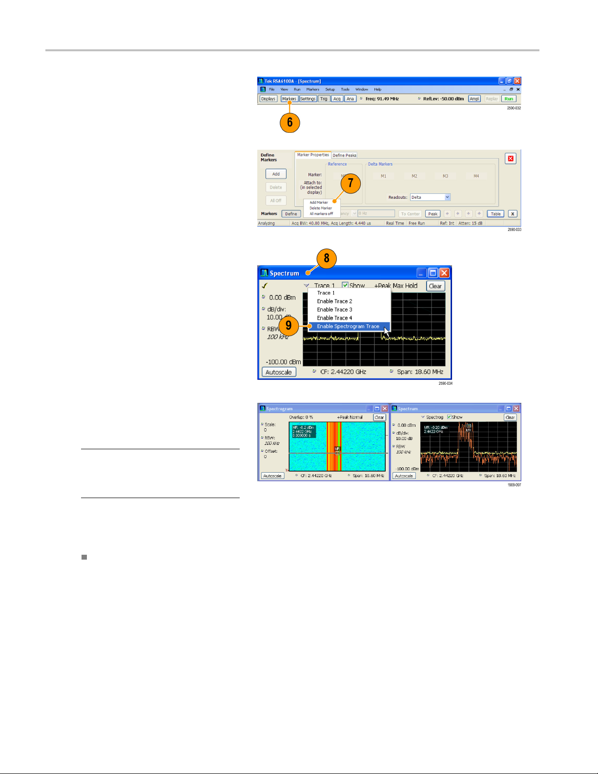
8. Click Markers in the application bar
to bring up the marker tool bar at the
bottom of the s
Do this with a mouse, by pressing
the screen with a finger, or push the
front-panel
9. Click Peak in the resulting marker toolbar
at the bottom
creen.
Markers P eak button.
of the display.
Application 1: M
aking a Basic Spectrum Measurement
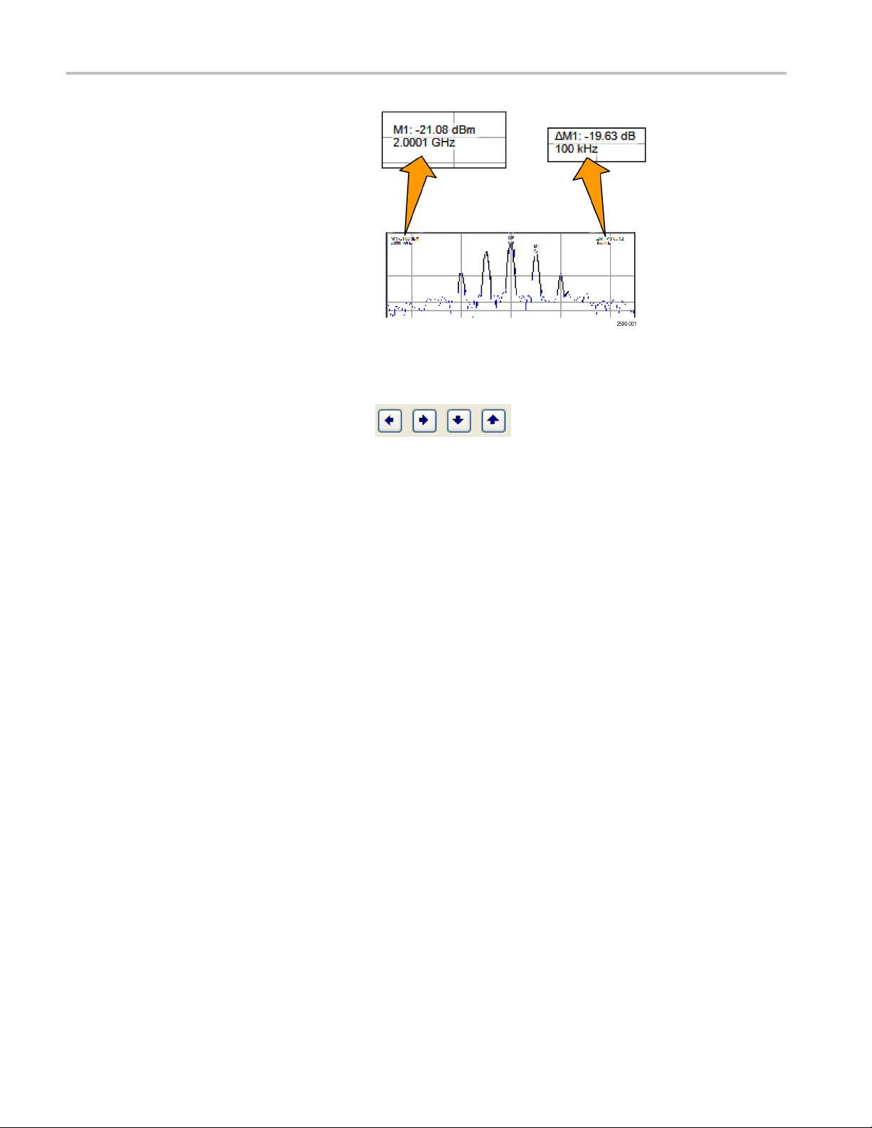
The instrum
highest level peak of the spectrum. It
displays the marker measurement in the
upper left
The first marker is labeled MR to indicate
that it is the reference marker.
10. Click M arkers Define in the bottom left
of the dis
This brings up the Define Markers
control panel.
11. Click Add.
A diamond shape labeled M1 appears o n
top of the MR marker and at the center
frequency. This is a delta marker.
The four delta markers, M1, M2, M3, and
M4, measure amplitude and frequency
referenced to MR.
You can also assign markers to specific
traces and adjust peak threshold.
12. Use your finger or the mouse to slide the
marker over to the next signal.
Alternatively, you can do the same task
with the knob or arrow key on the front
panel. Do this by assigning the control
to the marker by touching the marker
toolbar at the bottom of the screen.
ent places a marker on the
of the display.
play.
RSA6100A S eries & RSA5100A Series Application Examples Reference 3
Application 1: M
aking a Basic Spectrum Measurement
The marker read
shows the frequency and amplitude
differences between the reference
marker MR and t
The readout to the upper left shows the
absolute value of the M1 marker.
So far, you used m arkers to measure two
points of the same trace.
You can also use markers to measure further
differences between points. You can do this
by using the up, down, left, and right arrow
keys. You can also drag markers with the
mouse.
Alternatively, you can move markers by
rotating the front-panel knob or pressing the
front-panel arrow keys.
out at the upper right
he M1 delta marker.
4 RSA6100A Series & RSA5100A Series Application Examples Reference
Application 2: M
easuring Channel Power and Adjacent Channel Power
Application 2
: Measuring Channel Power and Adjacent
Channel Power
The RSA6100A and RSA5100A analyzers can take channel power, adjacent channel power, and multi-carrier channel
power measurements. This application demonstrates the settings used for taking channel power and adjacent channel
power measurements.
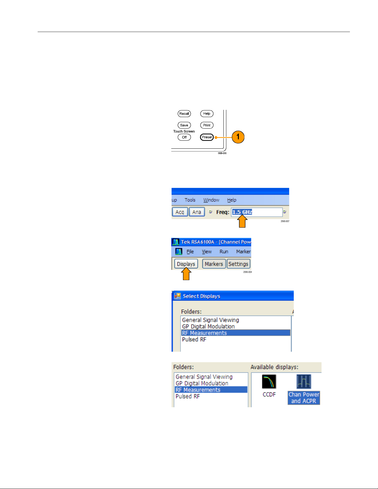
1. Push the front-panel Preset button to set
the instrument to the default settings.
Set up the appropriate measurement
parameters for the sample signal.
2. Ensure that Freq is set to 1.5 GHz.
3. Click Displays in the application bar.
Doing this will let you open the Channel
Power and ACPR display.
Alternatively, push the front-panel
Displays button.
4. Select the RF Measurements folder.
ble click or, alternatively, drag and
5. Dou
drop, the Channel Power and ACPR
icon in the Available displays area to
eittotheSelected displays area.
mov
RSA6100A S eries & RSA5100A Series Application Examples Reference 5
Application 2: M
easuring Channel Power and Adjacent Channel Power
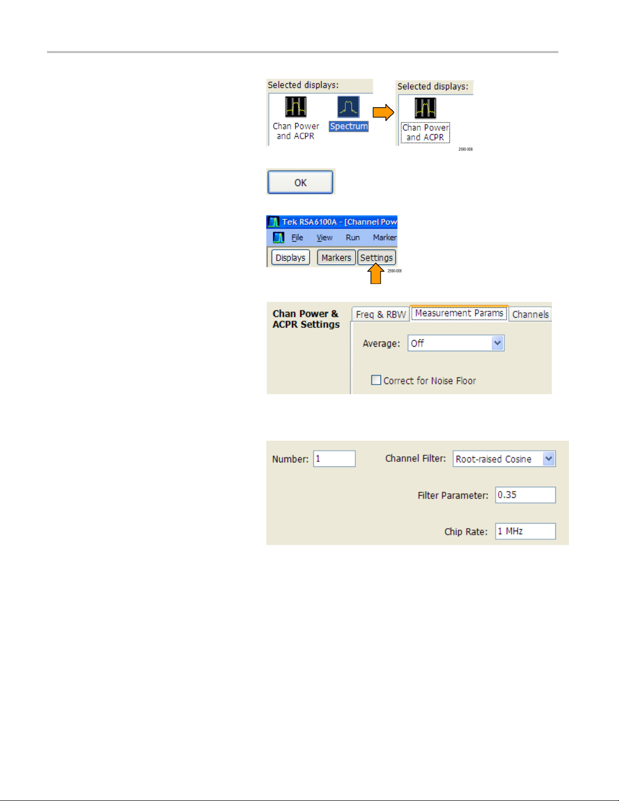
6. Double click, o
Spectrum icon to remove it from the
Selected displays area.
7. Click OK.
8. Click Settings in the application bar.
9. Click the Measurement Params tab.
For the pu
example, with its recalled signal, you can
leave the Average field as Off.
If you we
to use averaging, you want to select
Frequency Domain in the Average
field. Th
Leave Correct for Noise Floor
unchecked.
r drag and drop, the
rpose of this application
re using a live signal and wanted
at is a common setting.
10. Set Filter P arameter to 0.35.
11. Set Chip Rate to 1MHz.
ate is signal bandwidth.
Chip r
6 RSA6100A Series & RSA5100A Series Application Examples Reference
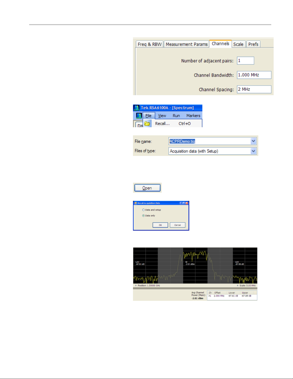
12. Click the Channels Tab. Use this to
define the channels to measure.
13. Ensure that the Number of adjacent
pairs is alrea
instrument to measure the main channel
and the one adjacent channel on each
side of it.
dy set to 1. This will set the
Application 2: M
easuring Channel Power and Adjacent Channel Power
14. Set Channel B
15. Set Channel
16. Select File
Do this to load the saved acquisition file.
17. Go to: C:/RSA6100A Files/Sam-
pleDataRecords or C:/RSA5100A
Files/SampleDataRecords.
Select Acquisition data asthetypeof
file to look for.
Select ACPRDemo.tiq as the file to
recall.
Click Open.
18. Select Data only and click OK.
Do not select Data and setup because
that would load control values that
were saved along with the acquisition
data. That would overwrite the settings
you made in the previous steps of this
application example.
andwidth to 1MHz.
Spacing to 2MHz.
> Recall
19. View the results.
The absolute channel power value
appears in the middle of the graph. The
upper adjacent power ratio appears to
the right, and the lower adjacent power
ratio appears to the left.
The gray-shaded bands illustrate the
space between channels. The analyzer
makes ACPR power measurements
within the defined channels, represented
by the unshaded black areas.
RSA6100A S eries & RSA5100A Series Application Examples Reference 7

Application 3: P
erforming Modulation Analysis
Application 3
The following example shows how to use your analyzer, with Option 21 installed, to demodulate a QPSK signal and to
analyze the signal in multiple domains. You will use the instrument to do the following:
Demodulate a QPSK signal to show its constellation diagram.
Measure the EVM (Error Vector Magnitude) and other key indicators using the Signal Quality display.
: Performing Modulation Analysis
8 RSA6100A Series & RSA5100A Series Application Examples Reference

Application 3: P
View the phase of the signal changing over time.
Use markers to see how the results correlate between the Symbol Table display, Constellation display, and the Phase vs
Time display.
NOTE. The following examples are based on the QPSK sample data file. If desired, you can load the QPSK sample data file
(QPSKDemo.tiq) to recreate the steps used in this application. The signal settings in the following examples are based on
the signal in
the sample file. If you use a live signal, your settings may differ.
erforming Modulation Analysis
Demodulate the Signal
1. Push the Pre
panel to set the instrument to the default
settings.
2. Tune the i
the span to 20 MHz. T hese settings are
appropriate for the signal that is analyzed
in this ex
3. Click Di
Displays dialog box.
4. Select the General Signal Viewing folder.
5. Select the Time Overview icon.
6. Click Add to add the Time Overview icon
to the Selected Displays list.
set button on the front
nstrument to 2.13 GHz and set
ample.
splays to open the Select
RSA6100A S eries & RSA5100A Series Application Examples Reference 9

Application 3: P
7. Select the GP Digital Modulation folder.
8. Select the EVM vs Time icon.
9. Click Add to add the icon to the Selected
Displays list.
10. Repeat steps 8 and 9 for the
Constellati
dialog box.
11. Select File > Recall.
erforming Modulation Analysis
on icon, and then close the
12. Go to: C:/RSA6100A Files/Sam-
pleDataRecords or C:/RSA5100A
Files/SampleDataRecords.
Select Acquisition data in the Files of
type field.
Select QPSKDemo.tiq in the File name
field.
Click Open. Select Data only in the
Recall Acquisition Data dialog and click
OK.
You might see a message on the display that
states Data acquired from data simulator .
This means that the sample data file
was generated, not captured from a live
acquisition.
Alternatively, you can use a live signal of
your own choice and reset the instrument
to match your signal’s parameters.
The General Purpose Digital Demodulation displays share the same modulation and advanced parameter controls. These
controls are available in the Settings control panel for each display.
10 RSA6100A Series & RSA5100A Series Application Examples Reference

13. Select the EVM vs Time display, and then
click Settings.
14. Select the Modulation tab.
15. Set the Modulation Type to QPSK.
16. Set the Symbol Rate to 3.84 MHz.
17. Set the Measurement Filter to
RootRaised
Cosine.
Application 3: P
erforming Modulation Analysis
18. Set the Ref
19. Set the Fil
20. Close the c
erence Filter to RaisedCosine.
ter Parameter to 0.220.
ontrol panel.
Analyze the Signal
You can analyze the signal using both qualitative and quantitative methods.
The Cons
to the illustration. You might need to click the
Autoscale button on the EVM vs Time display
to prop
QPSK signal, the points should be located in
four tight clusters. If they are not, check your
setti
Symbol Rate, and Filters.
Look at the trace in the EVM vs. Time
displ
percent at each trace point in time. The RMS
value for EVM during the entire analysis
peri
window, along with the peak EVM value and
the time (or symbol) at which it was detected.
tellation display should look similar
erly scale the graph display. For a
ngs for Frequency, Modulation Type,
ay. The graph shows the EVM value in
od is shown at the bottom of the display
RSA6100A S eries & RSA5100A Series Application Examples Reference 11

Application 3: P
Manually Adjust the Analysis Length
The Time Overview display shows the entire acquisition record, illustrating the length and offset for Spectrum Time and
Analysis Time. The spectrum length is the period of time within the acquisition record for which the spectrum is calculated.
The analysis length is the period of time within the acquisition record where other measurements are made. The analysis
length can be automatically determined by measurement parameters such as symbol rate, or you can manually adjust
the analysis length.
NOTE. The Spectrum Length and Spectrum Offset cannot be set independently unless the Spectrum Time Mode is set
to Independent. You can change the Spectrum Time Mode on the Analysis > Spectrum Time control panel tab. The red
line that represents the Spectrum Time settings in the Time Overview display is only shown when the Spectrum Time
Mode is set to Independent.
1. In the Time Overview display, select the
Analysis Length button.
The analysis length is indicated by the
blue bar above the graph.
2. Increase the analysis length to 500 us.
You can do this two ways: by changing
the value in the number entry box or by
dragging the right edge of the unshaded
area. Click Replay to rerun the analysis
using this new Analysis Length s etting.
Changing the Analysis Length setting
changes the amount of data used for
computing the measurements in the
displays. The shading in the display
shows the extent of the analysis period.
The increased analysis length causes
the instrument to automatically increase
the acquisition length setting to collect
enough samples to satisfy the new
analysis settings. By default, the
automatically determined acquisition
length is equal to or slightly greater than
the analysis length.
erforming Modulation Analysis
12 RSA6100A Series & RSA5100A Series Application Examples Reference

3. Select the Analysis Offset button.
4. Increase the Analysis Offset setting to
600 μs.
If the analysis offset is increased such
that the analysis period extends past
the end of the acquisition record, the
instrument will increase the acquisition
length to provide the additional data.
For a recalled signal, if you increase the
Analysis Length or Analysis Offset beyond
the end of the available data, the instrument
will analyze only the data that exists within
the set analysis period. To let you know
about the discrepancy, the instrument adds a
text readout to the right of the numeric value
readout stating actual: xx.x. usec.
Application 3: P
erforming Modulation Analysis
RSA6100A S eries & RSA5100A Series Application Examples Reference 13

Application 3: P
5. Change the Analysis Offset setting to
20μs.
6. Click Replay to update the measurement
results (you n
you m ake a change in Analysis O ffset or
Length when viewing recalled data).
erforming Modulation Analysis
eed to do this each time
7. Increase t
Because the instrument is stopped, it
cannot run a new acquisition to capture a
longer dat
analysis period extends past the end
of the data record, the actual analysis
length is
he analysis offset again.
a record. When the requested
reduced.
14 RSA6100A Series & RSA5100A Series Application Examples Reference

Application 4: P
erforming Time and Frequency Analysis
Application 4
The following example shows how to use your analyzer to measure frequency hops. You will use the instrument to do
the following:
Measure the transition time.
Measure the hop to hop frequency difference.
Measure the frequency overshoot.
View the spectrogram to see more detail in the frequency transitions versus time.
NOTE. The following examples were based on the TimeFrequency.tiq demonstration data file. If desired, you can load this
file to recreate the steps used in this application. The signal settings in the following examples were based on the signal in
the demonstration file. If you use a live signal, your settings may differ.
1. Click Displays.
This opens the Select Displays window.
: Performing Time and Frequency Analysis
2. Click Application Presets...
3. Click T
4. Click File and, from the resulting
ime-Frequency Analysis and
OK from the resulting window.
By using an application preset, you direct
strument to automatically do much
the in
of the setup work for you.
pull-down menu, click Recall....
alling a data fi le stops the instrument
Rec
from running new acquisitions so that
you can analyze the recalled data.
RSA6100A S eries & RSA5100A Series Application Examples Reference 15

Application 4: P
5. In the Open window, use the pull-down
Files of type control to select
Acquisition d
erforming Time and Frequency Analysis
ata (with Setup).
6. In the Look in
the path named C:/RSA6100A
Files/SampleDataRecords.or
C:/RSA5100
and click the file named
TimeFrequency.tiq.
7. Click Open.
8. Click Data only in the Recall Acquisition
Data dialo
This app
Frequency vs. Time, Time Overview,
Spectrogram, and Spectrum.
These di
both time- and frequency- domain
representations of hopping signals. They
e a reference marker (MR) and a
includ
delta marker (M1) to help measure the
hops.
field, navigate to
A Files/SampleDataRecords
g and click OK.
lication opens four displays titled
splays allow you to see
The Frequency vs Time display s hows
the deviation from the center frequency
on the vertical axis and time on the
value
horizontal axis.
pectrum display shows log power
The S
on the v ertical axis and frequency on the
horizontal axis.
16 RSA6100A Series & RSA5100A Series Application Examples Reference

The Spectrogram display shows time on
the vertical axis and frequency on the
horizontal ax
represents the amplitude at a particular
frequency at a particular time.
The Time Overview display shows log
power on the
the horizontal axis.
9. MovethemousetotheSpectrogram
display.
is. The color at each point
vertical axis and time on
Application 4: P
erforming Time and Frequency Analysis
10. Right click the mouse and select Zoom
from the resulting menu. Pull the mouse
lly and horizontally to zoom in
vertica
on one or two hops of the spectrogram
signal.
One way
graph is to think of it as a stack of
spectrum traces turned on edge.
to understand the spectrogram
RSA6100A S eries & RSA5100A Series Application Examples Reference 17

Application 4: P
erforming Time and Frequency Analysis
11. Use the mouse to
in the Spectrogram display to a point of
interest. As you move the marker up
and down, look
changes in the marker in the Spectrum
display. The Time-Frequency Analysis
application
Spectrum display to show the selected
spectrogram line.
As you contin
observe that the power remains constant
over time in the Time Overview display
even though
change over time in the Frequency vs
Time display.
The marker
between the Spectrum and Spectrogram
displays. The marker time is correlated
across the
Time,andTime Overview displays.
12. Show the full screen view of the
Frequency vs Time display. This will help
you more
carefully analyze the signal.
move the MR marker
at the corresponding
preset configured the
ue to move the marker,
you can see the frequency
frequency is correlated
Spectrogram, Frequency vs.
13. Click th
14. Cli
e right mouse button and select
Zoom from the mouse menu. Click and
hold the left mouse button and move the
o pull the displayed waveform
mouse t
out horizontally and vertically until you
have isolated one or two hops on the
n.
scree
Zooming in will help you see a more
detailed view of the signal and thus more
ately measure the overshoot. Now
accur
that you can see the signal and the
overshoot better, you c an also see that
ignal contains a lot of noise, which
the s
will impair your ability to measure the
overshoot. So the next step is to clear
e noise in the signal. One way to
up th
do that is to minimize the span setting
as far as you can.
ck Settings in the m enu bar.
18 RSA6100A Series & RSA5100A Series Application Examples Reference

15. Click Span in the resulting Frequency vs
Time Settings pane.
The span is the
control for all the measurements in the
General Signal Viewing folder, including
Frequency vs
of these displays will also change it in
the other displays.
16. Click the down arrow and see the setting
change to 20
Reducing the span decreases the
measurement bandwidth. Reducing
the measur
the amount of noise present on the
frequency vs. time waveform, allowing
for bette
transitions.
17. Click Replay.
Continue clicking Span, pushing the
down arr
up the signal more and more until the
waveform breaks down.
measurement bandwidth
. Time. Changing it in any
MHz.
ement bandwidth reduces
r resolution of the frequency
ow and clicking Replay to clean
Application 4: P
erforming Time and Frequency Analysis
Change the span settings to 10, 5, and
2MHz.A
breaks down and looks w rong, as shown
at the right. It no longer includes the hop
that y
When you set span too s mall, you
reduced the measurement bandwidth too
far.
result because you not only eliminated
unwanted noise but also eliminated
much
measure.
t 2 MHz, the waveform clearly
ou want to measure.
You invalidated the measurement
of the signal that you wanted to
RSA6100A S eries & RSA5100A Series Application Examples Reference 19

Application 4: P
erforming Time and Frequency Analysis
18. Push the up arro
span setting back to 10 MHz.
19. Click Replay to restore the good
waveform. You can see your desired
signal once ag
cleaner than it did at the original 40 MHz
setting.
Notice in the
now that you have cleaned up the signal,
you can clearly see a transient in it.
NOTE. To optimize the measurement
even further, you can go back to step 9
and use the right-button, mouse-controlled
Span Zoom and CF Pan features of the
Spectrogram display instead of the Zoom
and Pan features. Then use Replay and
Autoscale. Such an approach might yield a
further reduction of the span setting and thus
an even cleaner signal on which to make
your measurement.
w key twice to get the
ain, and it appears much
screen shot to the right that
20. Close th
pane.
21. Place the MR and M1 markers in the
Freque
one hop and measure hop frequency.
In the example to the right, the
hop-t
Marker MR is in the bottom plateau of the
waveform, and M1 is in the top plateau
of the
e Frequency vs Time Settings
ncyvsTimepane to enclose just
o-hop frequency is 2.094 MHz.
waveform.
20 RSA6100A Series & RSA5100A Series Application Examples Reference

Application 4: P
erforming Time and Frequency Analysis
22. Move the marker
The M1 marker is at the peak of the
overshoot, the MR marker is at the
middle of the h
overshoot is 370.240 kHz. The overshoot
occurs 151.600 μs before reference
marker MR.
23. Move the markers to measure transition
time. If yo
location of the markers, try using the
general purpose knob.
The trans
the signal is about to make a hop
and ends at about the settled time of
the new fr
measurements for your own application
might use other methods, such as
g when some other signal occurs
startin
or ending when the frequency has settled
to within some tolerance of a specified
cy.
frequen
The readout shows a 22.320 μs transition
time for a 1.919 MHz hop.
s to measure overshoot.
op frequency, and the
u have trouble fine-tuning the
itiontimeshownstartsas
equency. Transition time
RSA6100A S eries & RSA5100A Series Application Examples Reference 21

Application 5: C
apturing Transient Signals
Application 5
With the DPX Spectrum display, your analyzer can identify infrequently occurring transient signals and low-power signals that
may be obscured by stronger signals. After you find that these signals exist, you can use some of the following tools to
capture and examine the signal details to determine their cause:
Use the Max Hold function to verify the presence of signals other than the CW signal.
Use the DPX Spectrum display to view transient signals.
Create a frequency m ask and the use the Frequency Mask tri gger to capture any signal that violates the mask.
Use the Spectrogram with Frequency Mask Trigger to view the mask violations in the Time and Frequency domains.
Detecting Transient Signals Using the DPX Spectrum Display
The D PX Spe
signals so that you can see low-level and higher power signals that occur at the same frequency, but at different times.
1. Push the Preset button on the front
panel to s
default settings.
ctrum display uses a bitmap image in addition to line traces to view signals. Bitmaps can represent multi-value
et the instrument to the
: Capturing Transient Signals
2. Click Displays.
22 RSA6100A Series & RSA5100A Series Application Examples Reference

3. Select the General Signal Viewing
folder.
4. Select the DPX Spectrum icon.
5. Click Add to add the application to the
Selected Dis
plays list.
6. Select the Spectrum icon in the
d Displays list.
Selecte
Application 5: C
apturing Transient Signals
7. Click Re
move to clear the icon from
the list.
8. Close the dialog box.
RSA6100A S eries & RSA5100A Series Application Examples Reference 23

Application 5: C
apturing Transient Signals
9. Tune the instru
10. Adjust the spa
11. Select +Peak T
down menu. This new trace detects
the highest peaks in each DPX frame.
12. Click Settings to open the DPX
Spectrum Set
13. Click the Traces tab.
14. Select Hold from the Function list to
hold the peaks from all acquisitions.
15. Close the control panel.
ment to the signal.
n.
race from the drop
tings control panel.
Quick Tip
Click Clear located just above the graph to clear the display and start collecting points again.
The Hold function shows the highest points collected over continuing updates. Although the Hold trace shows the highest
it doesn’t show signals that are below the maximum value at any frequency. However, this is possible with the
points,
DPX bitmap trace.
24 RSA6100A Series & RSA5100A Series Application Examples Reference

16. Select Bitmap from the drop-down list.
17. Click Settings to open the DPX
Spectrum Settings control panel.
18. Enable Dot Persistence by checking its
box.
19. Increase the Variable Persistence
setting.
The more you increase the Persistence
setting, the more quickly you will see
infrequent signal events. In this example,
the more frequent signals appear in red;
infrequent signals will appear in blue.
Thesesettingscanalsobeusedtodisplay
signals below the maximum signal level. For
example, a low-level signal in the presence
of a pulsed signal might require a lower
Persistence and Intensity setting.
Application 5: C
apturing Transient Signals
RSA6100A S eries & RSA5100A Series Application Examples Reference 25

Application 5: C
Frequency Mask Triggering
If your instrument has Option 02/52 installed, you can use the Mask Editor to create a frequency mask for triggering on
transient signals. Complete the following steps to get a good visual reference that you can use to build the frequency mask.
1. Push the Preset button on the front
panel to set the instrument to the default
settings.
2. Tune the instrument to the frequency of
your signal.
3. Adjust the span.
4. Click Settings to open the Settings
control panel.
apturing Transient Signals
5. Select the Traces tab.
6. Select Trace 1 (make sure the Show
check box is checked).
7. Set the Detection to +Peak.
8. Set the Function to Max Hold.
9. Close the control panel.
26 RSA6100A Series & RSA5100A Series Application Examples Reference

10. Click Trig to open the Trigger control
panel.
11. SettheTypetoFrequency Mask.
12. Click Mask Editor to open the Mask
Editor.
13. Use the Mask Editor to create a mask
for your si
draw function and adjust if necessary.
Traces that you selected in the Spectrum
Analyzer
in the Mask Editor. All trace detections
and functions are available.
gnal. Start by using the Auto
display are used as references
Application 5: C
apturing Transient Signals
14. Close the Mask Editor.
15. Select the condition that you are
interested in.
For example, if you want the instrument
to trigger when it detects the first violati on
after seeing at least one acquisition with
no violations, select the F > T violation.
(A violation is when any point is within
the shaded mask area.)
16. Click Triggered.
The instrument should trigger when
a violation occurs. If you believe that
the instrument might have triggered
prematurely (on noise instead of a real
violation), then you might need to adjust
your mask to leave a wider margin
between the mask and your signal.
RSA6100A S eries & RSA5100A Series Application Examples Reference 27

Application 5: C
Viewing Transient Signals in Time and Frequency Domains
Spectrograms allow you to see how signals change over time. You can use the Spectrogram display to examine the transient
signals that violated the mask. Combining the Spectrogram display with the Frequency Mask Trigger allows you to see
how often the violations occur and to troubleshoot the cause of the problem.
1. Click Displays to open the Select
Displays dialog box.
2. Add the Spectrogram and Time Overview
displays.
3. Close the dialog box.
apturing Transient Signals
28 RSA6100A Series & RSA5100A Series Application Examples Reference

4. Select the Time Overview display.
5. Increase the Analysis Length setting until
the Time Overview display covers the
transient sig
nal.
Application 5: C
apturing Transient Signals
The Spec
of a transient signal. As you increase the
Analysis Length setting, the number of
spectro
also increases.
The marks along the right side of the
Spectr
each acquisition record.
trogram display shows an example
gram lines within each acquisition
ogram display show the beginning of
The Spectrogram display shows both time and frequency domains in a single display. The vertical axis is time, with newer
a at the bottom. The horizontal axis is frequency, covering the same span as the Spectrum display.
dat
RSA6100A S eries & RSA5100A Series Application Examples Reference 29
Application 5: C
6. Click Markers to open the M arker
toolbar.
7. Select Add M arker to add one marker
to the display.
8. Select the Spectrum display by clicking
the title b
apturing Transient Signals
ar.
9. Make sure t
Trace in the Spectrum display is checked.
The Spectrogram trace in the Spectrum
display
in the Spectrogram display by the active
marker.
NOTE. I
Spectrogram trace in the Spectrum display
shows first line from the analysis period in
rrent acquisition data record.
the cu
kTip
Quic
Spectrum traces 1, 2, 3, and 4 show the spectrum for the Spectrum Time selected in the Time Overview display or in the
Spectrum Time tab of the Analysis control panel. The Spectrogram, by comparison, covers the Analysis Time selected in
the Time Overview display or in the Analysis Time tab of the Analysis control panel.
he check box for Spectrogram
corresponds to the line selected
f there is no active marker, the
30 RSA6100A Series & RSA5100A Series Application Examples Reference

Application 6: Taking Pulse Measurements
Pulsed RF measurements have historically been difficult to perform. Some measurements required custom-built and
dedicated test tools, plus trained experts to properly use the tools to achieve accuracy and repeatability. Tektronix
real-time spectrum analyzers have revolutionized pulse measurements through automation. An RSA6100A Series or
RSA5100A Series Analyzer, with Option 20 installed, can replace specialized test equipment formerly required for pulsed
RF measurements.
This application shows how to accomplish the following pulsed RF measurement tasks:
Capture a series of RF pulses in a single acquisition record.
Select measurements to display in the Pulse Table.
Examine the pulse shape and measure reference points with the Pulse Trace display.
View Trend and FFT analysis on the measurement results with the Pulse Statistics display.
NOTE. To complete the following example, you will need a pulsed signal or an appropriate saved data record. This example
uses the PulseDemo.tiq file, which is located in the folder C:\RSA6100A Files\Sample Data Records or C:/RSA5100A
Files/SampleDataRecords.
Application 6: T
aking Pulse Measurements
Capture the Pulses
1. Push the Preset button on the front
panel to set the instrument to the default
settings.
2. Click Displays to open the Select
Displays dialog box.
RSA6100A S e ries & RSA5100A Series Application Examples Reference 31

Application 6: T
3. Select the General Signal Viewing folder.
4. Select the Time Overview icon and add
5. Select the Pulsed RF folder.
aking Pulse Measurements
the application to the Selected Displays
list.
6. Add the P ulse Table and Pulse Trace
s to the Selected Displays list.
display
7. Click OK
8. Set the F
9. Sele
Settings.
10. Set the Bandwidth valueto10MHz.
Close the Settings control panel.
to close the dialog box.
requency to 2.7 GHz.
ct the Pulse Trace display and click
32 RSA6100A Series & RSA5100A Series Application Examples Reference

11. Select File > Recall.
12. Go to: C:/RSA6100A Files/Sam-
pleDataRecords or C:/RSA5100A
Files/SampleDataRecords.
Select Acquisition data in the Files of
type field.
Select PulseDemo.tiq in the File name
field.
Click Open.
13. When the Recall Acquisition Data
window appears, select Data Only and
click OK.
Application 6: T
aking Pulse Measurements
atively, you can use a live signal of
Altern
your own choice and reset the instrument
to match your signal’s parameters.
14. In the Time Overview display, set the
sis Length to include several
Analy
pulses. Decrease the horizontal scale
to about 10 ms so you can see the first
e in detail. Adjust the Spectrum
puls
Offset so the Spectrum Time covers the
on time of this pulse.
15. Click Replay to run the measurements
r these new analysis and spectrum
ove
time periods.
16. Select the Pulse Table display and then
select Settings.
RSA6100A S eries & RSA5100A Series Application Examples Reference 33

Application 6: T
17. Select the Measurements tab.
18. Select the measurements that you are
19. Close the control panel.
20. When you see the data in the Pulse
Quick Tip
Measure the Parameters of the Captured Pulses
After you have captured the pulses, you can use the Pulse Trace display to view the details of specific measurements.
aking Pulse Measurements
interested in. (For this example, select
Average ON Pow
Rise Time).
Table display, click Replay to recalculate
the Pulse Ta
You can take measurements while the instrument is running or while it is stopped. Stopping the instrument may make it
easier to read the measurements from c aptured data.
er, Pulse Width, and
ble measurements.
1. Select o
ne of the measurement results
in the Pulse Table display. For example,
click the cell for the Width measurement
e1.
of Puls
The Pulse Trace display shows an
itude versus time trace for the
ampl
selected result on the selected pulse.
Blue lines and arrows show how the
urement was made.
meas
The green arrow in the display shows the
power threshold used to detect pulses. If
s threshold is set too high or too low,
thi
no pulses will be detected. You can set
the power threshold on the Settings >
ams tab.
Par
34 RSA6100A Series & RSA5100A Series Application Examples Reference

2. Click the Pulse control in the Pulse
Trace display and enter a different pulse
number.
The new pulse appears in the Pulse
Trace display and is selected in the
Pulse Table d
Pulse Trace display and the Pulse Table
display together to view and analyze
pulse measur
You can select a different result in the
Pulse Trace display and it will also be
selected in
isplay. You can use the
ements.
the Pulse Table display.
Application 6: T
aking Pulse Measurements
3. Use the Sca
zoom in on details of the selected pulse.
For example, you can adjust the controls
to get a cl
Rise Time measurement as shown.
le and Offset controls to
ose look at the details of the
Quick Tip
Click Autoscale to optimize the vertical and horizontal offset and scale settings.
When using scale or offset, adjust the offset control to move the area of interest to the far left side of the screen, and then
adjust the scale to expand the area of interest. Another way to change scaling is to right-click in the graph and select
Pan or Zoom, then use the mouse or the touchscreen to drag in the graph.
Review Measurement Statistics Across All Measured Pulses
an use the Pulse Statistics display to s how the trend or an FFT across all measured pulses. To get the best frequency
You c
resolution and dynamic range in the display, you need to include many pulses in the analysis period.
RSA6100A S e ries & RSA5100A Series Application Examples Reference 35

Application 6: T
1. Set the Analysis Length in the Time
2. Click Displays to open the Select
3. Select the Pulsed RF folder.
aking Pulse Measurements
Overview display to 19 ms.
Displays dialog box.
4. Remove the Spectrum icon and the
Time Overview icon from the Selected
Displays
5. Add the P
list.
ulse Statistics icon to the
Selected Displays list.
6. Close the dialog box.
36 RSA6100A Series & RSA5100A Series Application Examples Reference

Application 6: T
aking Pulse Measurements
When Trend is th
Pulse Statistics display plots the results
of the selected measurement for every
measured puls
7. Select the Φ Di
Pulse-to-pulse phase measurements are
good examples to show the trend and
FFT statisti
8. Change the St
FFT shows a spectrum-like trace of the
amplitude (in dB relative to the highest
result in t
can be useful for identifying interference
in the pulsed s ignal. For example, if a
spike appe
indicate coupling from the AC power
supply.
he set) versus frequency. This
e selected plot, the
e.
ff measurement.
cs.
atistics trace to FFT.
ars around 60 Hz, it might
RSA6100A S eries & RSA5100A Series Application Examples Reference 37
 Loading...