Tektronix RSA6106A, RSA6114A, RSA6120A, RSA5103A Online Help

Download

RSA6000 Series Real-Time Spectrum Analyzers

ZZZ

RSA5000 Series Real-Time Signal Analyzers

Printable Online Help

*P077051902*

077-0519-02

RSA6000 Series Real-Time Spectrum Analyzers RSA5000 Series Real-Time Signal Analyzers

ZZZ

PrintableOnlineHelp

www.tektronix.com

077-0519-02

Copyright © Tektronix. All rights reserved. Licensed software products are owned by Tektronix or its subsidiaries or suppliers, and are protected by national copyright laws and international treaty provisions.

Tektronix products are covered by U.S. and foreign patents, issued and pending. Information in this publication supersedes that in all previously published material. Speciﬁcations and price change privileges reserved.

TEKTRONIX and TEK are registered trademarks of Tektronix, Inc.

Online help version: 2.6

Contactin

Tektronix, Inc. 14150 SW Karl Braun Drive P. O . B o x 5 0 0 Beaverton, OR 97077 USA

For p roduct information, sales, service, and technical support:

g Tektronix

In North America, call 1-800-833-9200. Worldwide, visit www.tektronix.com to ﬁnd contacts in your area.

Table of Contents

Welcome

Welcome............................................................................................................. 1

About Tektronix Analyzers

Your Tektronix Analyzer........................................................................................... 3

Product Software ...................... ................................ .................................. ........... 4

Accessories

Standard Accessories.......................................................................................... 5

Recommended Accessories................................................................................... 6

Options

Options.......................................................................................................... 8

Documentation and Support

Documentation................................................................................................. 8

Table of Contents

Orientation

Front Panel Connectors ... ................................ .................................. ....................... 9

Front-Panel Controls .................................. ................................ ............................. 9

Touch Screen............................. .................................. ................................ ........ 13

Touch-Screen Actions............................................................................................. 13

Elements of the Display........................................................................................... 15

Rear-Panel Connectors............................................ .................................. .............. 19

Setting Up Network Connections . .... . .... . .... ..... .... . .... . .... ..... .... . .... . .... . .... .... . .... . .... ..... ... 19

Operating Your Instrument

Restoring Default Settings.............................. ................................ .......................... 21

Running Alignments .......... .................................. ................................ .................. 21

Presets. ................................ ................................ .................................. ............ 22

Setting Options. ..... ..... .... . .... . .... ..... ..... .... . .... . .... ..... ..... .... . .... . .... ..... ..... .... . .... . .... .... 27

Using the Measurement Displays

Selecting Displays ............. .................................. ................................ .................. 31

Taking Measurements

Measurements

Available Measurements ........... ................................ .................................. ........ 33

General Signal Viewing

Overview ........................................................................................................... 39

RSA6000 Series & RSA5000 Series Printable Online Help i

Table of Contents

DPX

DPX Primer ................................. .................................. ................................ 39

DPX Display Overview .......... ................................ .................................. .......... 62

DPX Display ...................... ................................ .................................. .......... 62

DPX Settings ... . .... . .... . .... ..... ... . . .... . .... . .... ..... ..... .... . .... . .... . .... . .... ..... ... . . .... . .... . .. 71

Time Overview

Time Overview Display...................................................................................... 86

Time Overview Settings ..................................................................................... 88

Spectrum

Spectrum Display ................. ................................ ................................ ............ 92

Spectrum Settings.. ..... .... . .... . .... .... . .... . .... .... . .... . .... .... . .... . .... .... . .... . .... .... . .... . .... .. 93

Spectrogram

Spectrogram Display ................. ................................ ................................ ........ 95

Spectrogram Settings . .... . .... . .... . .... ... . . .... . .... . .... .... . .... . .... ... . . .... . .... ..... ... . . .... . .... ... 98

Amplitude Vs Time

Amplitude Vs Time Display. ................................ .................................. ............ 102

Amplitude Vs Time Settings ............................ ................................ .................. 103

Frequency Vs Time

Frequency Vs Time Display ............................................................................... 104

Frequency Vs Time Settings.. . .... . .... . .... . .... . .... ..... ..... ..... ..... .... . ... . . .... . .... . .... . .... . .. 105

Phase Vs Time

Phase Vs Time Display..................................................................................... 106

Phase Vs Time Settings . .... . .... ..... ... . . .... . .... . .... .... . .... . .... . .... . .... .... . .... . .... ..... ..... .. 107

RF I & Q Vs Time

RF I & Q vs Time Display................................................................................. 108

RF I & Q vs Time Settings.. . .... . .... . .... ..... . .... ..... ..... ..... ..... ..... ..... .... . ..... .... . .... . .... 109

Common Controls for General Signal Viewing Displays

General Signal Viewing Shared Measurement Settings ... . .... . .... ... . . .... . .... .... . .... . .... ... . . .. 110

Analog Modulation

Overview ......................................................................................................... 121

AM Display ....................... ................................ .................................. ........ 121

AM Settings ................................................................................................. 122

FM Display .................................................................................................. 128

FM Settings.. . .... . .... .... . .... . .... . .... . .... .... . .... . .... . .... ..... .... . .... . .... ..... .... . .... . .... . .... 130

PM Display .................................................................................................. 136

PM Settings.. . .... . .... .... . .... . .... . .... . .... .... . .... . .... . .... ..... .... . .... . .... ..... .... . .... . .... . .... 138

ii RSA6000 Series & RSA5000 Series Printable Online Help

RF Measurements

Overview ......................................................................................................... 145

Channel Power and ACPR

Channel Power and ACPR (Adjacent Channel Power Ratio) Displ

Channel Power and ACPR Settings .. ................................ ................................ .... 148

MCPR

MCPR (Multiple Carrier Power Ratio) Display . . .... ..... .... . .... . .... .... . .... . .... .... . .... . .... .... 151

MCPR Settings.............. ................................ ................................ ................ 154

Occupied BW & x dB BW

Occupied BW & x dB BW Display................. ................................ ...................... 160

Occupied BW & x dB BW Settings ........ ................................ .............................. 163

Spurious

Spurious Display............................................................................................ 164

Spurious Display Settings. .... . .... . .... . .... ..... ..... .... . .... . .... . .... . .... . .... . .... ..... ..... .... . ... 168

CCDF

CCDF Display............................................................................................... 175

CCDF Settings . . .... ... . . .... . .... ... . . .... . .... ... . . .... . .... ..... .... . .... . .... ... . . .... . .... ... . . .... . ... 176

Phase Noise

Phase Noise Display........................................................................................ 178

Phase Noise Settings . . .... . .... ..... ..... .... . .... . .... . .... . .... . .... . .... ..... ..... .... . .... . .... . .... . .. 181

Settling Time Measurements

Settling Time Measurement Overview .. . . .... . .... . .... ..... .... . .... . .... ... . . .... . .... . .... ..... .... . . 184

Settling Time Displays

Settling Time Displays . .... ..... ... . . .... . .... . .... ..... .... . .... . .... . .... ... . . .... . .... . .... . .... .... . ... 188

Settling Time Settings .. . .... . .... . .... . .... . .... . .... ..... ..... .... . .... . .... . .... . .... ..... ..... .... . .... . 195

Common Controls for Settling Time Displays

Settling Time Displays Shared Measurement Settings ..... .... . .... . .... . .... ..... .... . .... . .... . .... . 195

SEM (Spectrum Emission Mask)

SEM Display ................................................................................................ 203

Spectrum Emission Mask Settings .... . .... ..... .... . .... . .... . .... . .... .... . .... . .... . .... . .... ..... ... . . 206

Common Controls for RF Measurements Displays

RF Measurements Shared Measurement Settings . .... ... . . .... . .... . .... ..... .... . .... . .... ..... ... . . .. 213

Table of Contents

ay................................ 145

OFDM Analysis

Overview ......................................................................................................... 221

OFDM Chan Response

OFDM Channel Response Display ....................................................................... 221

OFDM Channel Response Settings ... .... . .... . .... . .... . .... ..... ..... .... . .... . .... . .... . .... . .... ..... 223

OFDM Constellation

OFDM Constellation Display ............................................................................. 224

OFDM Constellation Settings ... ..... ..... .... . .... . .... . .... . .... . .... . .... . .... . .... ..... ..... ..... ..... 225

OFDM EVM

RSA6000 Series & RSA5000 Series Printable Online Help iii

Table of Contents

OFDM EVM Display .. .................................. ................................ .................. 225

OFDM EVM Settings .... ..... .... . .... . .... ..... .... . .... . .... ... . . .... . .... ..... ... . . .... . .... ..... .... . . 226

OFDM Mag Error

OFDM Magnitude Error Display ......................................................................... 227

OFDM Magnitude Error Settings......................................................................... 228

OFDM Phase Error

OFDM Phase Error Disp

OFDM Phase Error Settings . . .... . .... ... . . .... . .... . .... ..... .... . .... . .... ..... ..... .... . .... . .... ... . . . 230

OFDM Power

OFDM Power Display ..................................................................................... 231

OFDM Power Settings .... . .... . .... . .... .... . .... . .... . .... . .... .... . .... . .... . .... . .... .... . .... . .... . ... 232

OFDM Summary

OFDM Summary Display.................... ................................ .............................. 233

OFDM Summary Settings ................................................................................. 235

OFDM Symb Table

OFDM Symbol Table Display............................................................................. 236

OFDM Symbol Table Settings . .... . .... . .... ... . . .... . .... ..... .... . .... . .... .... . .... . .... ... . . .... . .... 237

Common Controls for OFDM Analysis Displays

OFDM Analysis Shared Measurement Settings .... ..... .... . .... . .... . .... ..... .... . .... . .... . .... ..... 237

lay ......... ................................ .................................. .... 229

Pulsed RF

Overview ......................................................................................................... 245

Pulse Table Display

Pulse Table Display......................... ................................ ................................ 245

Pulse Table Settings .... .... . .... . .... ..... .... . .... . .... . .... .... . .... . .... . .... ..... .... . .... . .... ..... ... 246

Pulse Trace Display

Pulse Trace Display........................................... .................................. ............ 247

Pulse Trace Settings .... .... . .... . .... ..... ..... .... . .... . .... ..... ..... .... . .... . .... ..... ..... .... . .... . .. 249

Pulse Statistics

Pulse Statistics Display..................................................................................... 249

Pulse Statistics Settings .................................. .................................. ................ 251

Common Controls for Pulsed RF Displays

Pulsed RF Shared Measurement Settings .... . .... . .... . .... . .... .... . .... . .... . .... . .... .... . .... . .... . . 251

Audio Analysis

Overview ......................................................................................................... 263

Audio Spectrum

Audio Spectrum Display ................................................................................... 263

Audio Spectrum Settings..... .... . .... . .... .... . .... . .... . .... ..... .... . .... . .... ... . . .... . .... . .... ..... .. 264

Audio Summary

Audio Summary Display................... ................................ ................................ 265

Audio Summary Settings . .... . .... ..... .... . .... . .... . .... ..... .... . .... . .... . .... ... . . .... . .... . .... . .... 266

iv RSA6000 Series & RSA5000 Series Printable Online Help

Common Controls for Audio Analysis Displays

Audio Analysis Measurement Settings ................................................................... 267

GP Digital Modulation

Overview ......................................................................................................... 277

Constellation

Constellation Display....................................................................................... 278

Constellation Settings .... .... . .... . .... .... . .... . .... ..... ... . . .... . .... ..... .... . .... . .... ... . . .... . .... .. 279

Demod I & Q vs Time

Demod I & Q vs Time Display............................................................................ 280

Demod I & Q vs Time Settings ........................................................................... 282

EVM vs Time

EVM vs Time Display........ ................................ .................................. ............ 282

EVM vs Time Settings ..... .... . .... . .... ..... ..... .... . .... . .... ..... .... . .... . .... . .... .... . .... . .... . ... 283

Eye Diagram

Eye Diagram Display............................. ................................ .......................... 284

Eye Diagram Settings .... . .... . .... . .... . .... . .... . .... . .... . .... ..... . .... ..... ..... ... . . ..... .... . .... . .. 285

Frequency Deviation vs Time

Frequency Deviation vs Time Display ................................................................... 286

Frequency Deviation vs Time Settings .... . .... . .... . .... . .... . .... ..... ..... .... . .... . .... . .... . .... . ... 288

Magnitude Error vs Time

Magnitude Error vs Time Display .. ................................ .................................. .... 288

Magnitude Error vs Time Settings .... ................................ .................................. .. 290

Phase Error vs Time

Phase Error vs Time Display ...................... .................................. ...................... 290

Phase Error vs. Time Settings ... .... . .... . .... . .... . .... . .... . .... ..... ..... .... . .... . .... . .... . .... . .... . 292

Signal Quality

Signal Quality Display ................... ................................ ................................ .. 292

Signal Quality Settings .... . .... ..... ..... .... . .... . .... . .... . .... ..... ..... .... . .... . .... . .... . .... ..... ... 297

Symbol Table

Symbol Table Display ............................ ................................ .......................... 298

Symbol Table Settings. .... . .... ..... . .... ..... ..... ..... ..... ... . . ..... .... . .... . .... . .... . .... . .... . .... . . 299

Trellis Diagram

Trellis Diagram Display.. . .... . .... .... . .... . .... . .... ..... .... . .... . .... ... . . .... . .... . .... ..... .... . .... . 299

Trellis Diagram Settings .... . .... ..... .... . .... . .... .... . .... . .... ... . . .... . .... .... . .... . .... ... . . .... .... 301

Common Controls for GP Digita l Modulation Displays

GP Digital Modulation Shared Measurement Settings ................................................. 301

Standard Settings Button......... ................................ .................................. ........ 302

Symbol Maps

Symbol Maps................ ................................ .................................. .............. 317

User Filters

Overview: User Deﬁned Measurement and Reference Filters. .... . .... . .... .... . .... . .... . .... ..... .. 323

Table of Contents

RSA6000 Series & RSA5000 Series Printable Online Help v

Table of Contents

User Filter File Format .. . .... . .... . .... ... . . .... . .... . .... . .... .... . .... . .... . .... . .... .... . .... . .... . .... . 324

Marker Measurements

Using Markers

Using Markers............................................................................................... 327

Controlling Markers with the Touchscreen Actions Menu .... ..... .... . .... . .... ..... ... . . .... . .... . .. 327

Measuring Signal Density, Frequency and Power on a DPX Bitmap Trace.......................... 328

Measuring Frequency and Power in the Spectrum Display .......... ................................ .. 330

Common Marker Actions

Marker Action Controls... ................................ .................................. .......... 331

Peak................................ ................................ .................................. .... 331

Next Peak ............................................................................................... 331

Marker to Center Frequency.......................................................................... 331

Deﬁne Markers Control Panel

Enabling Markers and Setting Marker Properties . . .... ..... ..... .... . .... . .... . .... ..... .... . .... . 331

Markers Toolbar

Using the Markers Toolbar.............................. ................................ .............. 333

Noise Markers in the Spectrum Display

Using Noise Markers in the Spectrum Display............. ................................ ........ 334

Search (Limits Testing)

The Search Tool (Limits Testing).............. .................................. .............................. 337

Search (Limits Te

Deﬁne Tab (Search) ....... ................................ ................................ ...................... 337

Actions Tab......................... .................................. ................................ ............ 342

sting) Settings .... ..... .... . .... . .... . .... . .... . .... . .... ... . . .... . .... . .... . .... . .... . .... .. 337

Analyzing Data

Analysis Settings

Analysis Settings.. .... . .... . .... ... . . .... . .... ..... ... . . .... . .... ..... .... . .... . .... .... . .... . .... . .... ... . . 343

Analysis Time Tab.......................................................................................... 343

Spectrum Time Tab............... ................................ .................................. ........ 345

Frequency Tab............................................................................................... 345

Units Tab............................. ................................ .................................. ...... 349

Analyzing Data Using Replay

Replay Overview ........................................................................................... 349

Replay Menu ................................ .................................. .............................. 352

Acq Data......................... ................................ ................................ ............ 352

DPX Spectra................................................................................................. 352

Replay All Selected Records .......................... .................................. .................. 353

Replay Current Record..................................................................................... 353

Replay from Selected....................................................................................... 353

Pause ............. ................................ .................................. .......................... 353

vi RSA6000 Series & RSA5000 Series Printable Online Help

Stop........................................................................................................... 353

Select All .................................................................................................... 353

Select Records from History............................................................................... 354

Replay Toolbar .............................................................................................. 354

Amplitude Corrections

Amplitude Settings . ..... .... . .... . .... . .... . .... ..... ..... .... . .... . .... . .... . .... ..... ..... .... . .... . .... . .... . 357

Internal Settings Tab . . .... ..... .... . .... . .... ... . . .... . .... ... . . .... . .... ... . . .... . .... ... . . .... . .... ... . . .... . . 357

External Gain/Loss Correction Tab.......................................... ................................ .. 360

External Gain Value ........................................................................................ 361

Apply External Corrections To.................... ................................ ........................ 361

External Loss Tables ....................................................................................... 362

ernal Probe Correction Tab................................................................................. 364

Ext

Controlling the Acquisition of Data

Acquisition Controls in the Run Menu

Continuous Versus Single Sequence............................ .................................. ........ 365

Run ................. ................................ ................................ .......................... 365

Resume....................................................................................................... 365

Abort ............. ................................ .................................. .......................... 365

Acquisition Controls in the Acquire Control Panel

The Acquire Control Panel .................................... .................................. .......... 366

Sampling Parameters Tab.................... ................................ .............................. 366

Advanced Tab (Acquire)................................................................................... 368

FastSave ..................................................................................................... 369

FastSave Tab ................................................................................................ 371

UsingTriggerstoCaptureJustWhatYouWant

Triggering

Triggering............................................................................................... 371

Frequency Mask Trigger .................. ................................ ............................ 375

Mask Editor (Frequency Mask Trigger) ....................... .................................. .... 375

Trigger Settings .............. ................................ .................................. ........ 379

Event Tab ............................................................................................... 379

Time Qualiﬁed Tab .................................................................................... 388

Advanced Tab (Triggering) ........................... ................................ ................ 389

Actions Tab (Triggering) .............................................................................. 391

Table of Contents

Managing Data, Settings, and Pictures

Saving and Recalling Data, Settings, and Pictures.. . .... ..... .... . .... . .... ..... .... . .... . .... .... . .... . .... 3 93

Data, Settings, and Picture File Formats .... ..... .... . .... . .... ..... .... . .... . .... .... . .... . .... ... . . .... . .... 396

Printing Screen Shots ....................... ................................ ................................ .... 400

RSA6000 Series & RSA5000 Series Printable Online Help vii

Table of Contents

Reference

Online Help ...................................................................................................... 401

About the Tektronix RTSA..................................................................................... 401

Connecting Signals

Conﬁgure In/Out Settings.. . .... .... . .... ..... .... . .... ..... .... . .... ..... .... . .... ... . . .... . .... .... . .... . 402

Connecting an RF Signal .................................................................................. 402

Connecting a Signal Using a TekConnect Probe .............. .................................. ........ 404

Connecting External Trigger Signals ..................................................................... 405

Digital I/Q Output .......... ................................ .................................. .............. 405

IQ Outputs ..................... ................................ ................................ .............. 405

Analog IF Output ........................................................................................... 406

Other Outputs ............................................................................................... 407

Menus

Menu Overview............................................................................................. 407

File Menu

View Menu

Run Menu

Replay

Markers Menu

Setup Menu

Tools Menu

Window Menu

Help Menu

Troubleshooting

Error and Information Messages .......... .................................. .............................. 419

Displaying the Windows Event Viewer .................................................................. 428

Dealing with Sluggish Instrument Operation............................................................ 429

On/Standby Switch

On/Standby Switch ....................... ................................ .................................. 429

Upgrading the Instrument Software

How to Find Out If Instrument Software Upgrades Are Available.................................... 430

Changing Settings

File Menu ............................................................................................... 408

More Presets............................................................................................ 412

View Menu ............................................................................................. 412

Run Menu......................................... ................................ ...................... 414

Replay Menu ........................................................................................... 415

Markers Menu.......................................................................................... 415

Setup Menu................. ................................ ................................ ............ 415

Tools Menu ....................... ................................ ................................ ...... 416

Arranging Displays .................................................................................... 418

Help Menu .......... .................................. ................................ .................. 419

viii RSA6000 Series & RSA5000 Series Printable Online Help

Glossary

Index

Table of Contents

Settings. .... . .... . .... . .... . .... . ..... .... . ..... ... . . ..... ..... ..... ..... ..... ..... ..... ..... . .... ..... . .... .. 430

RSA6000 Series & RSA5000 Series Printable Online Help ix

Table of Contents

x RSA6000 Series & RSA5000 Series Printable Online Help

Welc ome Welc ome

Welcome

This help provides in-depth information on how to use the RSA6000 Series Real-Time Spectrum Analyzers and RSA5000 S eries Real-Time Signal Analyzers. This online help contains the most complete description the RSA6000 Series Real Time Spectrum Analyzer and RSA5000 Series Real-Time Signal Analyzer Quick Start User Manual. To see tutorial examples of how to use your analyzer to take measurements in different application areas, refer to the RSA6000 Series Real Time Spectrum Analyzer and RSA5000 Series Real-Time Signal Analyzer Application Examples Reference.

s of how to use the analyzer. For a shorter introduction to the spectrum analyzer, refer to

RSA6000 Series & RSA5000 Series Printable Online Help 1

Welc ome Welcome

2 RSA6000 Series & RSA5000 Series Printable Online Help

About Tektronix Analyzers Your Tektronix Analyzer

Your Tektronix Analyzer

The RSA6000 Series and RSA5000 Series Analyzers will help you to easily discover design issues that other signal analyzers may miss. The revolutionary DPX display offers an intuitive live color view of signal transients c your design, or instantly displaying a fault when it occurs. This live display of transients is impossible with other signal analyzers. Once a problem is discovered with DPX, the Tektronix Analyzers can be set to trigger on the event, capture a continuous time record of changing RF events and perform time-correlated analysis in all domains. You get the functionality of a wideband vector signal analyzer, a spectrum analyzer and the unique trigger-capture-analyze capability of a Real-Time Analyzer – all in a single package.

Discover

hanging over time in the frequency domain, giving you immediate conﬁdence in the stability of

RSA6000 S (option 110 + option 200), 24 μs (option 200).

RSA5000 (standard); 10.3 μs (option 85 + option 200), 24 μs (option 200).

eries: DPX Minimum Event Time Capture: 24 μs (option 110), 31 μs (standard); 10.3 μs

Series: DPX Minimum Event Time Capture: 24 μs (option 85), 31 μs (option 40), 31 μs

Trigger

RSA6000 Series: Tektronix exclusive 40 MHz and 110 MHz DPX Density and Frequency Mask triggers offer easy event-based capture of transient RF signals by triggering on any change in the frequency domain.

RSA5000 Series: Tektronix exclusive 25 MHz, 40 MHz, and 85 MHz DPX Density and Frequency Mask triggers offer easy event-based capture of transient RF signals by triggering on any change in the frequency domain.

Capture

A6000 Series: All signals within a 110 MHz bandwidth span are captured into memory (Option

RS 110 only, 40 MHz acquisition bandwidth standard).

SA5000 Series: All signals within a 85 MHz bandwidth span are captured into memory (Option 85

R only, 40 MHz acquisition bandwidth with Option 40, and 25 MHz standard).

RSA6000 Series: Up to 1.7 seconds acquisition length at 110 MHz bandwidth provides complete analysis over time w ithout making multiple acquisitions.

RSA5000 Series: Up to 7 seconds acquisition length at 85 MHz bandwidth provides complete analysis over time without making multiple acquisitions.

RSA6000 Series & RSA5000 Series Printable Online Help 3

About Tektronix Analyzers Product Software

Analyze

Extensive time-correlated m ulti-domain displays connect problems in time, frequency, phase and amplitude for quicker understanding of cause and effect when troubleshooting.

Power measurements and signal statistics help you characterize components and systems: ACLR, Multi-Carrier ACLR, Power vs. Time, CCDF, Phase Noise, and Spurious.

Advanced Measurement Suite (Opt. 20): Pulse measurements including rise time, pulse width, duty, ripple, power, frequency and phase provide deep insight into pulse train behavior.

General Purpose Digital Modulation Analysis (Opt. 21): Provides vector signal analyzer functionality.

Product Software

The instrument includes the following software:

RSA6000 Series System Software: The RSA6000 Series product software runs on a specially conﬁgured version of Windows XP. As with standard Windows XP installations, you can install other compatible applications, but the installation and use of non-Tektronix software is not supported by Tektronix. If you need to reinstall the operating system, follow the procedure in the Restoring the Operating System chapter in the RSA6000 Series Real-Time Spectrum Analyzers Service manual

ronix p art number 077-0250-XX). You can download a PDF version of the Service manual

(Tekt at www.tektronix.com/manuals provided by Tektronix for use with your instrument.

. Do not substitute any version of Windows that is not speciﬁcally

RSA5000 System Software: The RSA5000 Series product software runs on Windows 7. As with standard Windows 7 installations, you can install other compatible applications, but the installation and use of non-Tektronix software is not supported by Tektronix. If you need to reinstall the operating system, follow the procedure in the Restoring the Operating System chapter in the RSA5000 Series Real-Time Signal Analyzers Service manual (Tektronix part number 077-0522-XX). You can

wnload a PDF version of the Service manual at www.tektronix.com/manuals

do version of Windows that is not speciﬁcally provided by Tektronix for use with your instrument.

roduct Software: The product software is the instrument application. It provides the user interface

P (UI) and all other instrument control functions. You can minimize or even exit/restart the instrument application as your needs dictate.

Occasionally new versions of software for your instrument may become available at our Web site. Visit

www.tektronix.com/software

for information.

. D o not substitute any

Software and Hardware Upgrades

Tektronix may offer software or hardware upgrade kits for this instrument. Contact your local Tektronix distributor or sales ofﬁce for more information.

4 RSA6000 Series & RSA5000 Series Printable Online Help

About Tektronix Analyzers Standard Accessories

Standard Accessories

The standard accessories for the RSA6000 Series and RSA5000 Series instruments are shown below. For the latest information on available accessories, see the Tektronix Web site

Quick Start User Manual

English - Op

Japanese - Option L5, Tektronix part number 071-2840-XX

Russian, Option L10, Tektronix part number 071-2841-XX

Simpliﬁed Chinese - Option L7, Tektronix part number 071-2839-XX

tion L0, Tektronix part number 071-2838-XX

Applications Instructions

English – Tektronix part number 071-2834-XX

Simpliﬁed Chinese - Option L7, Tektronix part number 071-2835-XX

Japanese - Option L5, Tektronix part number 071-2836-XX

Russian, Option L10, Tektronix part number 071-2837-XX

Product Documentation CD-ROM

The Product Documentation CD-ROM contains PDF versions of all printed manuals. The Product Documentation CD-ROM also contains the following manuals, some of which are available only in PDF format:

RSA6000 Series Declassiﬁcation and Security Instructions manual PDF, Tektronix part number 077-0170-XX

RSA5000 Series Declassiﬁcation and Security Instructions manual PDF, Tektronix part number 077-0521-XX

RSA6000 Series Service Manual PDF, Tektronix part number 077-0250-XX

RSA5000 Series Service Manual PDF, Tektronix part number 077-0522-XX

RSA6000 Series and RSA5000 Series Programmer Manual PDF, Tektronix part number 077-0523-XX

RSA6000 Series Speciﬁcations and Performance Veriﬁcation PDF, Tektronix part number 077-0251-XX

RSA5000 Series Speciﬁcations and Performance Veriﬁcation PDF, Tektronix part number 077-0520-XX

Other related materials

RSA6000 Series & RSA5000 Series Printable Online Help 5

About Tektronix Analyzers Recommended Accessories

NOTE. To check for updates to the instrument documentation, browse to www.tektronix.com/manuals and search by your instrument's model number.

Important Documents Folder

Certiﬁcate o

f Calibration documenting NIST traceability, 2540-1 compliance, and ISO9001 registration

Power Cords

North America - Option A0, Tektronix part number 161-0104-00)

Universal

United Kingdom - Option A2, Tektronix part number 161-0104-07

Australia - Option A3, Tektronix part number 161-0104-05

240V North America - Option A4, Tektronix part number 161-0104-08

Switzerland - Option A5, Tektronix part number 161-0167-00

Japan - Option A6, Tektronix part number 161-A005-00

China -

India - Option A11, Tektronix part number 161-0324-00

No power cord or AC adapter - Option A99

cal Wheel Mouse

Opti

Euro - Option A1, Tektronix part number 161-0104-06

Option A10, Tektronix part number 161-0306-00

Product Software CD

Recommended Accessories

The recommended accessories for the RSA6000 Series and RSA5000 Series instruments are shown in the following table. For the latest information on available accessories, see the Tektronix Web site

6 RSA6000 Series & RSA5000 Series Printable Online Help

About Tektronix Analyzers Recommended Accessories

Item

Additional Re

movable Hard Drive for use with RSA6000 Series Option 06 (Windows XP and instrument software installed)

Additional Removable Hard Drive for use with RSA5000 Series Optio

n 56 (Windows 7 and instrument software

installed)

Transit Case

Rackmount I

nstallation Kit

Additional Quick Start User Manual (paper)

Additional Documents CD (all manuals in PDF format)

xxx

Ordering part n

065-0751-XX

065-0852-00

016-2026-X

RSA56KR

071-2838-

063-4314-

umber

RSA6000 Series & RSA5000 Series Printable Online Help 7

About Tektronix Analyzers Options

Options

To view a listing of the software options installed on your instrument, select Help > About Your Tektronix Real-Time Analyzer. There is a label on the rear-panel of the instrument that lists installed

hardware opt

Options can be added to your instrument. For the latest information on available option upgrades, see the Tektron

ions.

ix Web site

Documentation

In addition to the online help, the following documents are available:

Quick Start User Manual (071-2838-XX - English). The Quick Start User Manual has information about installing and operating your instrument. The Quick Start User Manual is also available in Simpliﬁed Chinese (071-2839-XX), Japanese (071-2840-XX), and Russian (071-2841-XX).

Application Examples Reference (071-2834-XX). The Application Examples Reference provides examples of speciﬁc application problems and how to solve those problems using an RSA6000 Series

um analyzer. The Application Examples Reference is also available in Simpliﬁed Chinese

spectr (071-2835-XX), Japanese (071-2836-XX), and Russian (071-2837-XX).

Progra

which is located on the Documents CD. See the Documents CD-ROM for installation information.

Servi

manual is provided as a printable PDF ﬁle, which is located on the Documents CD. See the Documents CD-ROM for installation information. The Service manual includes procedures to service the instrument to the module level and restore the operating system.

Speciﬁcations and Performance Veriﬁcation Technical Reference Manual (RSA6000 Serie s: 077-0251-XX, RSA5000 Series: 077-0520-XX). This is a PDF-only manual that includes both the speciﬁcations and the performance veriﬁcation procedure. It is located on the Documents CD.

Declassiﬁcation and Security Instructions (RSA6000 Series: 077-0170-XX, RSA5000 Series: 077-0521-XX) This document helps customers with data security concerns to sanitize or remove memory devices from the instrument. It is located on the Documents CD.

The most recent versions of the product documentation, in PDF format, can be downloaded from

www.tektronix.com/manuals

mmer Manual (077-0523-XX). The Programmer Manual is provided as a printable PDF ﬁle,

ce Manual (RSA6000 Series: 077-0250-XX, RSA5000 Series: 077-0522-XX). The Service

.Youcanﬁnd the manuals by searching on the product name.

Other Documentation

Your instrument includes supplemental information on CD-ROM:

Documents CD (Tektronix part number 063-4314-XX)

8 RSA6000 Series & RSA5000 Series Printable Online Help

Orientation Front Panel Connectors

Front Panel Connectors

Fron

Item

2TrigIn

xxx

Connector

Trig Out Trigger output connector. 50 Ω, BNC, High > 2.0 V, Low < 0.4 V, (output

USB 1.1 USB 1.1 Mouse connector.

USB 2.0 USB 2.0 connector.

RF Input

t-Panel Controls

Descripti

current 1 mA).

External Trigger input connector, –2.5 V to +2.5 V (user settable).

RF input connector 50 Ω.

Left: RSA6000 Series, Right: RSA5000 Series

RSA6000 Series & RSA5000 Series Printable Online Help 9

Orientation Front-Panel Controls

Reference

Item Function Menu Equivalent

1 Media DVD-RW or removable hard disk

drive.

2 Displays

Opens the Disp

lays dialog box enabling you to select which displays to open.

4 Trigger

Settings Opens/closes the Settings control

panel for th

Opens/clos

e selected display.

es the Trigger control panel. O n the RSA5000 Series, this button lights when the trigger mode is set to Tr

Acquire

Opens/cl

iggered.

oses the Acquire control

panel.

6 Analysis

Opens/closes the Analysis control panel.

Freq Press to adjust the measurement

frequency.

Span (Spectrum)

Press to adjust the span or press and hold to display the Freq & Span

l panel for the General Signal

contro Viewing displays.

9Amplit

ude

Opens/closes the Amplitude control panel.

BW (Spectrum)

Press to adjust the bandwidth or press and hold to display the BW

rol panel for the General Signal

cont Viewing displays.

xxx

Setup > Displa

Setup > Settings

Setup > Trig

Setup > Ac

ger

quire

Setup > Analysis

Setup > Analysis > Frequency

Setup > Amplitude

Left: RSA6000 Series, Right: RSA5000 Series

10 RSA6000 Series & RSA5000 Series Printable Online Help

Orientation Front-Panel Controls

Reference

Item Function Menu Equivalent

11 Tab Moves the cursor to the next entry

in the dialog b

ox or control panel. Same as pressing the Tab key on an external keyboard.

12 Run

Peak (Markers section)

Starts and stops acquisitions. Run > Start Run > Stop

Moves the active marker to the maximum peak of the trace in the selected di

splay. If markers are turned off, the marker reference (MR) will appear at the maximum peak.

Select (Markers section)

Selects the next marker. If markers are turned

off, the MR marker (marker reference) will appear.

Deﬁne (Markers section)

Opens the Markers control panel. If markers are turned off, the MR marker (r

eference) will appear.

16 Esc Exits a dialog box without saving

changes

: the same as Esc on an

external keyboard.

Control knob Changes values in numeric and list

controls. Pressing the knob (clicking

he same as pressing the Enter

it) is t key on a keyboard.

18 Arrow

keys

he Markers. The Up arrow

Move t moves the selected marker to the next highest peak. The down arrow

the selected marker to the

moves next lower peak value. The right and left arrows move the selected marker

e next peak.

to th

Incr ment keys

20 Mar

ement/decre-

kers, Delete

Increments or decrements the

cted value

sele

etes the selected marker

Del

21 Markers, Add Add a marker to the selected trace

22 Replay Replays the current acquisition record

Single Sets the Run mode to Single

Sequence

xxx

Markers > Peak

RSA6000 Series & RSA5000 Series Printable Online Help 11

Orientation Front-Panel Controls

Reference

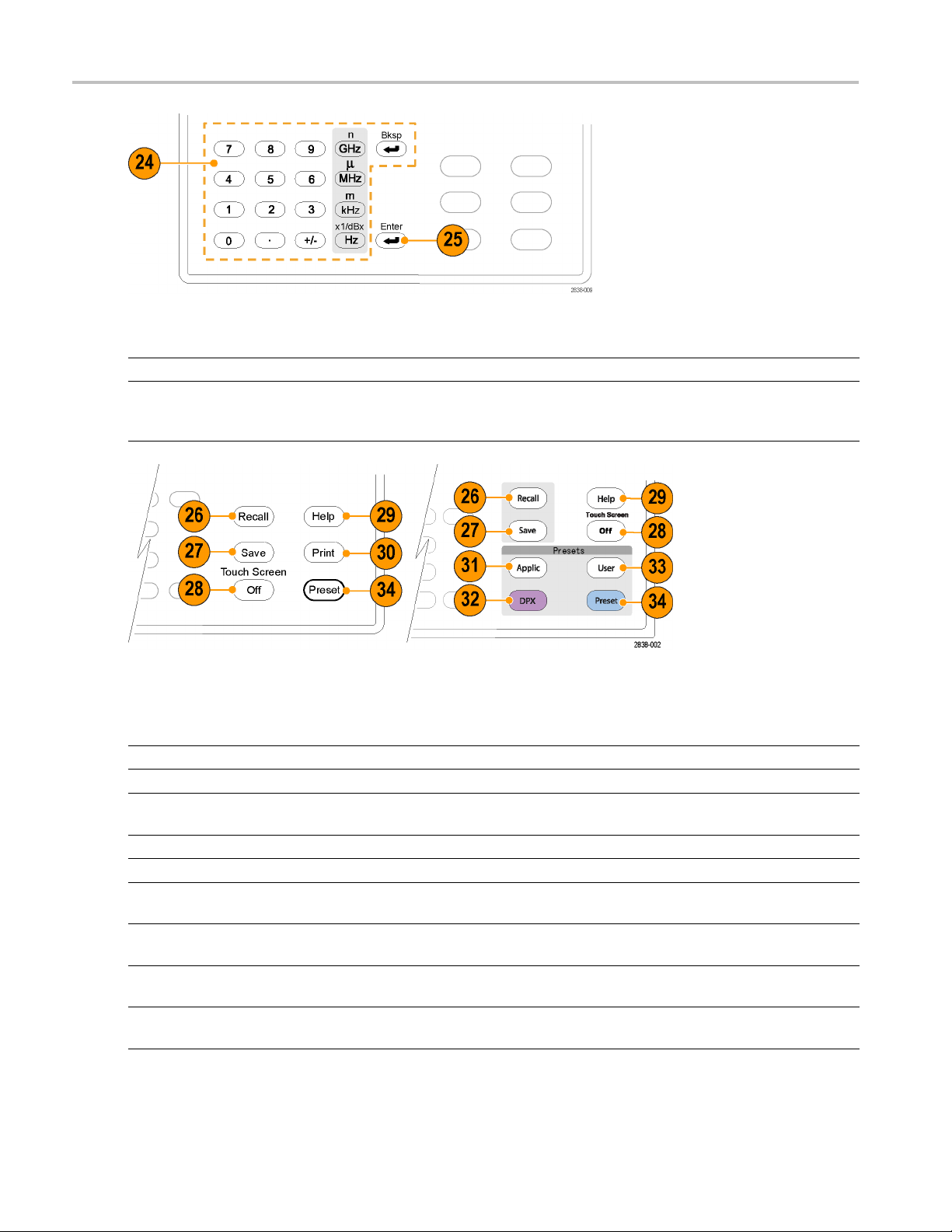
Item Function Menu Equivalent

24 Keypad Enters values in numeric controls.

25 Enter

Completes data entry in controls. Same as pressing the Enter key on an external keyboard.

xxx

Left: RSA6000 Series, Right: RSA5000 Series

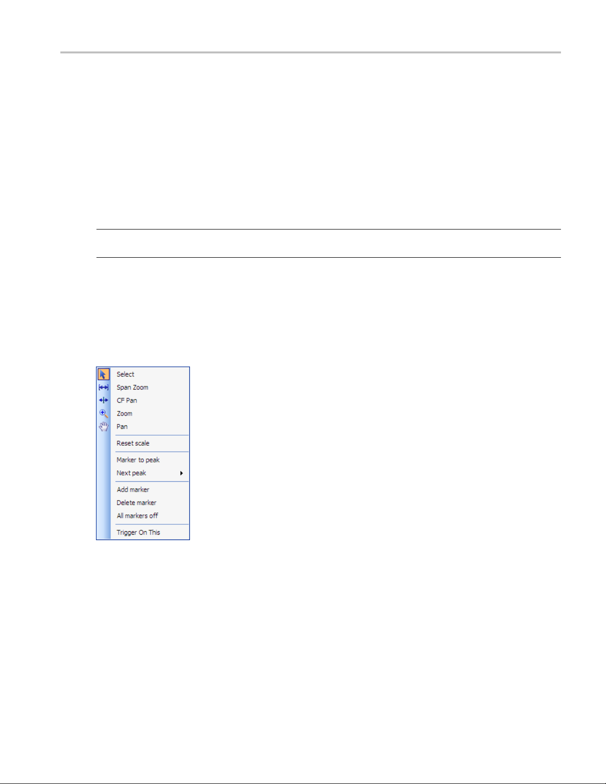
Reference

26 Recall

29 Help Displays the online help.

30 Print Displays the Print dialog box. File > Print

31 Applic

32 DPX

33 User

34 Preset

xxx

Item Function Menu Equivalent

Opens the Recall dialog box.

File > Recall

Save Opens the Save As dialog box. File > Save As

Touch Screen Off Turns the touch screen on and off. It

is off when lighted.

Help > Online Manual

Sets the instrument to the selected

Setup > More Presets > Application

Application Preset values.

Sets the instrument to the selected

Setup > More Presets > DPX

DPX Preset values.

Sets the instrument to the selected

Setup > More Presets > User

User Preset values.

Returns the instrument to the default

Setup > Preset

or preset values.

12 RSA6000 Series & RSA5000 Series Printable Online Help

Orientation Touch Screen

Touch Screen

You can use touch to control the instrument in addition to the front-panel controls, mouse, or extended keyboard. Generally, touch can be used anywhere that click is mentioned in this online help.

To disable the touch screen, push the front-panel TouchScreenOffbutton. When the touch screen is off, the button is lighted. You can still access the on-screen controls with a mouse or keyboard.

You can adjust the touch screen operation to your personal preferences. To adjust the touch screen settings, from Windows, select Start > Control Panel > Touch Screen Calibrator.

NOTE. If th need to use a mouse or keyboard to restore normal operation.

Touch-S

You can u Touch-screen Actions menu.

e instrument is powered on in Windows Safe Mode, the touch screen is inoperative. You will

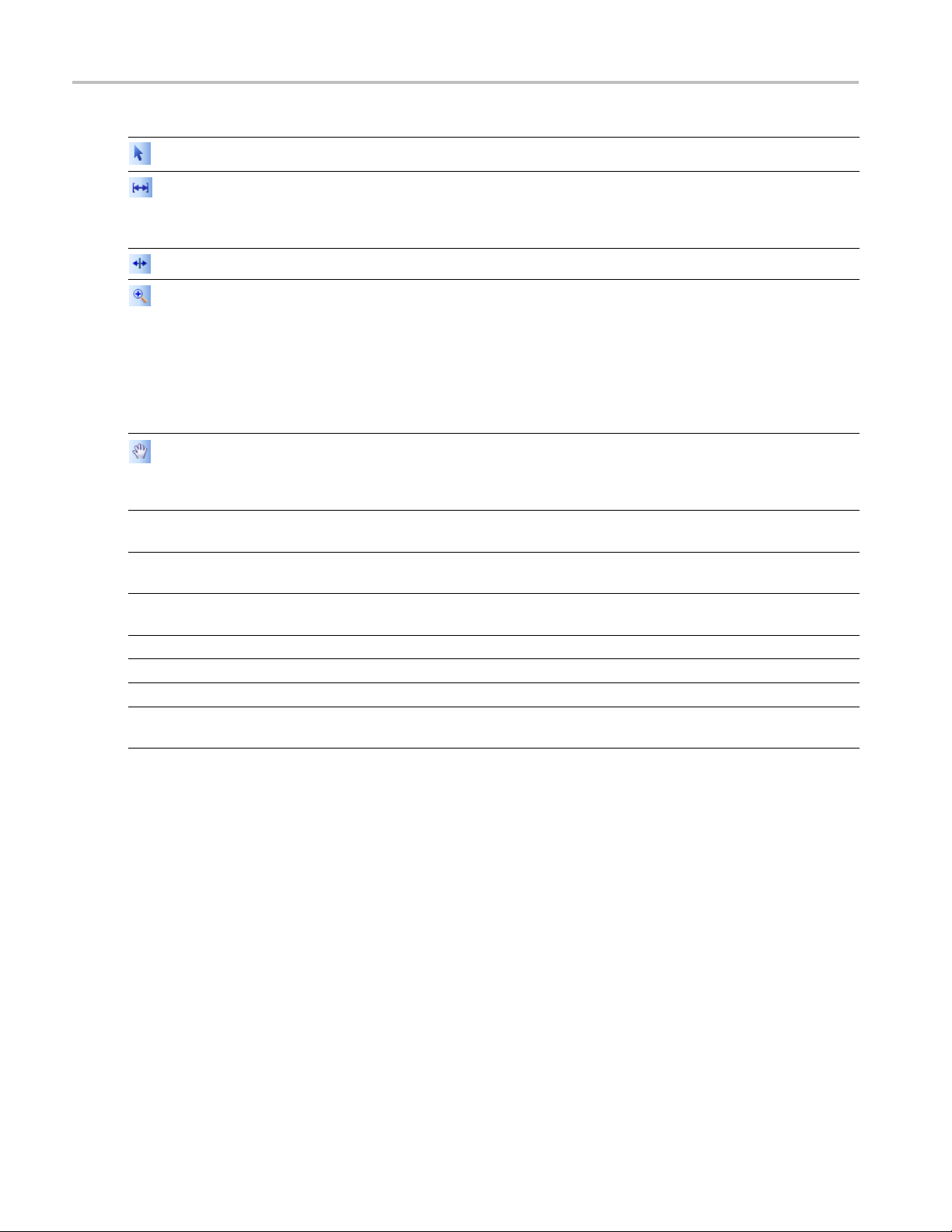
creen Actions

se the touch screen to change marker settings and how waveforms are displayed by using the

To use the Touch-screen Actions menu, touch the display in a graph area and hold for one second, then remove your ﬁnger. You can also use a mouse to display the Touch-screen Action menu by clicking the right mouse button.

RSA6000 Series & RSA5000 Series Printable Online Help 13

Orientation Touch-Screen Actions

Icon Menu Description

Select Selects markers and adjusts their position.

Span Zoom

CF Pan Adjusts the Center Frequency according to horizontal movement.

Zoom

Pan

xxx

ch-Screen Menu for Spurious Display

Tou

Reset Scale

Marker to peak

Next Peak

Add marker

Delete marker Removes the last added marker.

All markers off

Trigger On This Use to visually deﬁne trigger parameters in the DPX display

Zooms the graph area about the selected point. Touch the graph display at a point of interest and drag to increase or decrease the span about the point of interest. Span Zoom adjusts the span control and can affect the acquisition bandwidth.

Adjusts horizontal and vertical scale of the graph. The ﬁrst direction with enough movement becomes the primary scale of adjustment. Adjustment in the secondary direction does not occur until a threshold of 30 pixels of movement is crossed.

Dragging to the left or down zooms out and displays a smaller waveform (increases the scale value). Dragging to the right or up zooms in and displays a larger waveform (decreases the scale value).

Adjusts horizontal and vertical position of the waveform. The ﬁrst direction with enough movement becomes the primary direction of movement. Movement in the secondary direction does not occur until a threshold of 30 pixels of movement is crossed.

Returns the horizontal and vertical scale and position settings to their default values.

Moves the selected marker to the highest peak. If no marker is turned on, this control automatically adds a marker.

Moves the selected marker to the next peak. Choices are Next left, Next right, Next lower (absolute), and Next higher (absolute).

Deﬁnes a new marker located at the horizontal center of the graph.

Removes all markers.

(present only in the DPX Spectrum display).

The Touch-screen actions menu in the Spurious display has some minor changes compared to the standard

rsion used in other displays.

14 RSA6000 Series & RSA5000 Series Printable Online Help

Orientation Elements of the Display

Icon Menu Description

xxx

Single-range Changes the current multi-range display to a single range display.

The displayed range is the range in which you display the touchscreen-actions menu. Selecting Single-range from the menu is equivalent to selecting Single on the Settings > Parameters tab.

Multi-range

Marker -> Sel Spur

Changes the current single-range display to a multi-range display. Selecting Multi-range from the menu is equivalent to selecting Multi on the Settings > Parameters tab.

Moves the selected marker to the selected spur.

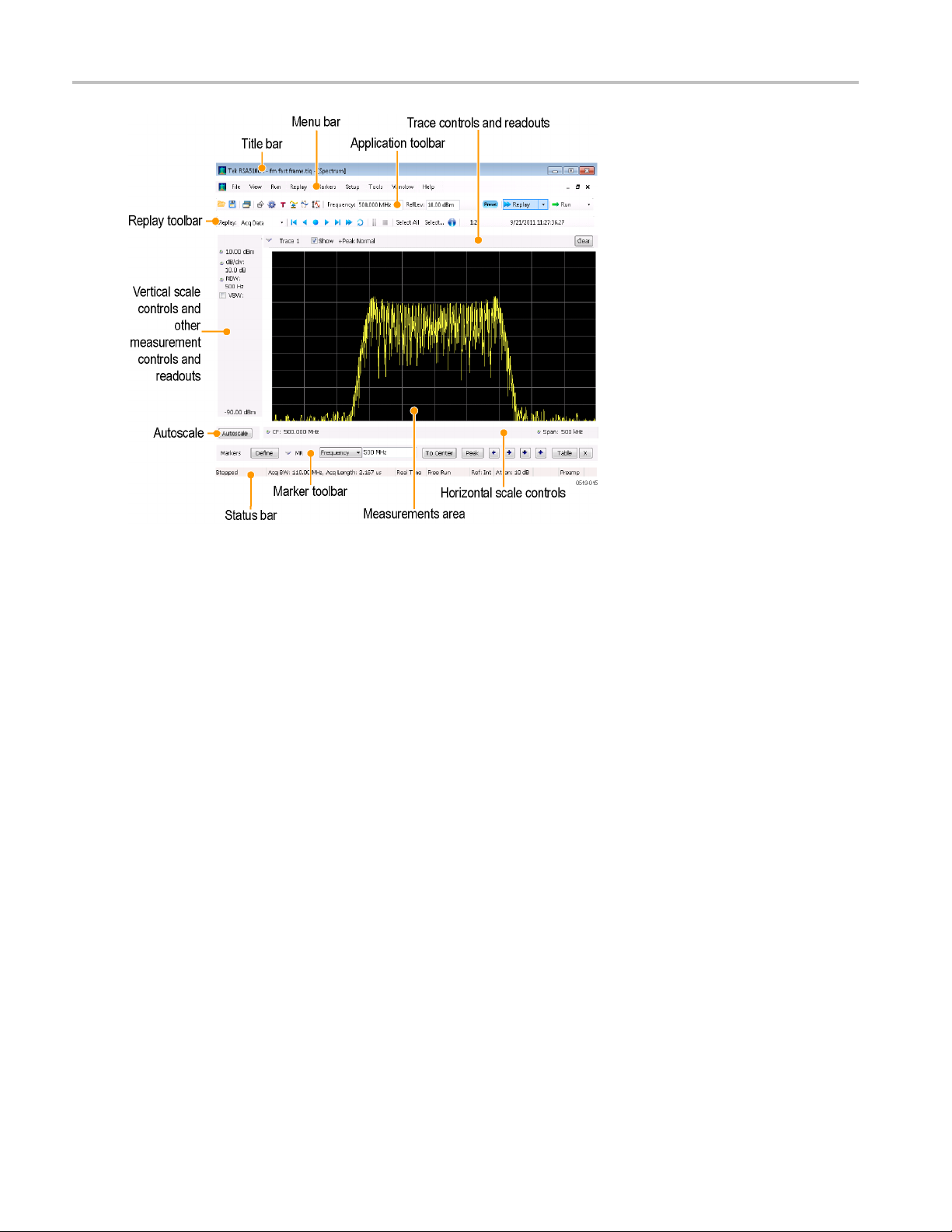
Elements of the Display

The main areas of the application window are shown in the following ﬁgure.

RSA6000 Series & RSA5000 Series Printable Online Help 15

Orientation Elements of the Display

Speciﬁc

elements of the display are shown in the following ﬁgure.

16 RSA6000 Series & RSA5000 Series Printable Online Help

Orientation Elements of the Display

RSA6000 Series & RSA5000 Series Printable Online Help 17

Orientation Elements of the Display

Ref

Setting

number

1 Displays

2Markers

Settings Opens the Settings control panel for the selected display. Each display has

4 Trigger

Acquire

6 Analysis

Frequenc

Reference Level Displays the reference level. To change the value, click the text and enter a

9 Amplitude

10 Repla

11 Ru n

13 Re

xxx

ck mark indicator

Che

call

Save Opens the Save As dialog in order to save setup ﬁles, pictures (screen

reset

Description

Opens the Select Displays dialog box so that you can select measurement displays.

Opens or closes the Marker toolbar at the bottom of the window.

its own cont

Opens the Tr

Opens the A

Opens the

rol panel.

igger control panel so that you can deﬁne the trigger settings.

cquire control panel so that you can deﬁne the acquisition settings.

Analysis control panel so that you can deﬁne the analysis settings

such as frequency, analysis time, and units.

Displays the frequency at which measurements are made. For spectrum displays, this is called “Center Frequency”. To change the value, click the text and

use the front panel knob to dial in a frequency. You can also enter a frequency with the front panel keypad or use the front panel up and down buttons.

number

Opens

from the keypad or use the front panel up and down buttons.

the Amplitude control panel so that you can deﬁne the Reference Level,

conﬁgure internal attenuation, and enable/disable the (optional) Preampliﬁer.

new measurement cycle on the last acquisition data record using any

Runs a new settings.

Starts and stops data acquisitions. When the instrument is acquiring data, the button label has green lettering. When stopped, the label has black lettering.

an specify the run conditions in the Run menu. For example, if you

You c select Single Sequence in the Run menu, when you click the Run button, the instrument will run a single measurement cycle and stop. If you select

tinuous, the instrument will run continuously until you stop the acquisitions.

Con

check mark indicator in the upper, left-hand corner of the display indicates

The the display for which the acquisition hardware is optimized.

Displays the Open window in order to recall setup ﬁles, acquisition data ﬁles, or trace ﬁles.

aptures), acquisition data ﬁles, or export measurement settings or acquisition

c data.

Recalls the Preset (Main)

(see page 416) preset.

18 RSA6000 Series & RSA5000 Series Printable Online Help

Orientation Rear-Panel Connectors

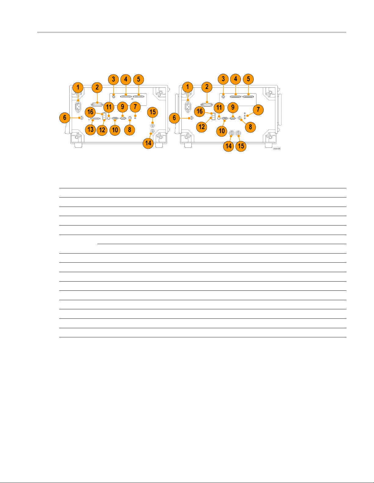
Rear-Panel Connectors

Left: RSA6000 Series, Right: RSA5000 Series

Item Descripti

4,5

8 Trig2 ln

16 Ethernet network connector

xxx

AC Input,

GPIB

IF Outpu

Real Ti

+28 V DC

RSA60

RSA5

COM 2, serial port for connecting peripherals

VGA external monitor output

PS2 keyboard input

USB2.0 ports for mouse and other peripherals (printers, external hard disks)

Unused connector (RSA6000 Series only)

Ref Out, reference frequency output

Ref In, reference frequency input

main power connector

t (optional)

me IQ Output (optional)

Output, switched

00 Series: Headphone, audio output connector

000 Series: Microphone in; Headphone, audio output; and Line In connectors

Setting Up Network Connections

Because the instrument is based on Windows, you conﬁgure network connections for the instrument the samewayyouwouldforanyPCbasedonWindows.SeeHelp and Support in the Windows Start menu to access the Windows Help System for information on setting up network connections.

RSA6000 Series & RSA5000 Series Printable Online Help 19

Orientation Setting U p Network Connections

20 RSA6000 Series & RSA5000 Series Printable Online Help

Operating Your Instrument Restoring Default Settings

Restoring Default Settings

To restore the instrument to its factory default settings:

Select File > Preset (Main) to return the analyzer to its default settings.

Preset resets all settings and clears all acquisition data. Settings and acquisition data that have not been saved will be lost.

Running Alignments

Alignments are adjustment procedures. Alignments are run by the instrument using internal reference signals and measurements and do not require any external equipment or connections.

There are two settings for Alignments:

Automatically align as needed

Run alignments only when the Align Now button is pressed

If Automatically align as needed is selected, alignments run whenever the spectrum analyzer detects asufﬁcient change in ambient conditions to warrant an alignment.

If Run alignments only when "Align N ow" button is pressed is selected, the spectrum analyzer never runs an alignment unless you manually initiate an alignment using the Align Now button.

NOTE. There a re a few critical adjustments that must run occasionally even if Automatically align is not enabled.

Alignment Status

When the spectrum analyzer needs to run an alignment, it displays a message on screen. If no message is displayed, you can assume that the spectrum analyzer is properly aligned.

NOTE. If you must use the instrument before it has completed its 20-minute warm-up period, y ou should perform an alignment to ensure accurate measurements.

Initiating an Alignment

1. Select Setup > Alignments.

2. Select the Align Now button.

The spectrum analyzer will run an alignment procedure. Status messages are displayed while the alignment procedure is running. If the instrument fails the alignment procedure, an error message will be

RSA6000 Series & RSA5000 Series Printable Online Help 21

Operating Your Instrument Presets

displayed. If the instrument fails an alignment, run Diagnostics (Tools > Diagnostics) to see if you can determine why the alignment failed.

NOTE. While an

Alignments during warm-up. During the 20-minute warm-up period, the spectrum analyzer will use the

alignment d (if Auto mode is selected). During the speciﬁed period for warm-up, the instrument performance is not warranted.

Alignments during normal operation. Once the spectrum analyzer reaches operating temperature, a n

alignment will be run. If an alignment becomes necessary during a measurement cycle (if Auto mode is selected completed, the measurement cycle restarts.

NOTE. The ﬁrst time the instrument runs after a software upgrade (or reinstall), the instrument will perform a full alignment after the 20–minute w arm-up period. This alignment cannot be aborted and it occurs even if alignments are set to run only when manually initiated.

Align

Alignments are adjustment procedures run by the instrument using internal reference signals and meas traceable test equipment (signal sources and measuringequipment)toverifytheperformanceofthe instrument.

), the measurement is aborted and an alignment procedure is run. Once an alignment procedure is

ments Are Not Calibrations

urements. Calibrations can only be performed at a Tektronix service center and require the use of

alignment is running, both the IF and IQ outputs are disabled.

ata generated during the previous use of the instrument as it warms to oper ating temperature

Presets

Menu Bar: File > More presets > Preset options

e analyzer includes a set of conﬁgurations or presets that are tailored to speciﬁc applications. These

Th conﬁgurations, referred to as Presets, open selected displays and load settings that are optimized to address speciﬁc application requirements. There are three types of factory Presets: Main, Application, and DPX. In addition to these factory deﬁned Presets, you can create your own Presets, called User Presets, you can recall to conﬁgure your analyzer.

22 RSA6000 Series & RSA5000 Series Printable Online Help

Operating Your Instrument Presets

Application Preset Description

Modulation Analysis The Modulation Analysis setup application preset provides you with the most common

displays used during modulation analysis. On ly present when Option 21 is installed.

Pulse Analysis The Pulse Analysis application preset provides you with the most common displays used

during pulse analysis, and makes changes to the default parameters to settings better optimized for

Spectrum Ana

Spur Search Multi Zone 9k-1GHz

Time-Frequency Analysis

DPX Preset Description

Swept The DPX Swept Preset displays the D PX Spectrum display with the center frequency

Zero Spa

Main Pre

Curren

nal: V1.0 – V2.3

Origi

User Description

Preset 1

User

User Preset 2

xxx

lyzer

n (Option 200 only)

sets

t: V2.4 and later

The Spectrum for general purpose spectrum analysis.

The Spur Search application preset conﬁgures the instrument to show the Spurious display with the frequency range set to 9 kHz to 1 GHz.

The Time-Frequency preset conﬁgures the instrument with settings suited to analyzing signal beh

set to 1.5

The DPX Z frequency set to 1.5 GHz and the sweep set to 1 m s.

Descrip

This Pr to show a Spectrum display with settings appropriate for typical spectrum analysis tasks. This preset was updated from the original factory preset with version 2.4 of the instru

This P This version of the factory preset is included to allow users to maintain compatibility with existing remote control software.

This Preset is provided as a example for you to create your own Presets. This preset displays the Spectrum, Spectrogram, Frequency vs Time, and Time Overview displays.

This Preset is provided as a example for you to create your own Presets. This preset

plays the Spurious display conﬁgured to test for Spurious signals across four ranges.

dis

pulsed signal analysis. Only present when Option 20 is installed.

Analysis application preset provide you with the settings commonly used

aviorovertime.

GHz and the span set to 3 GHz.

ero Span Preset displays the DPX Zero Span display with the center

tion

eset sets the instrument to display a Spectrum display with settings matched

ment software.

reset is the original factory preset used with software versions 1.0 through 2.3.

Modulation Analysis

The Modulation Analysis application preset opens the following displays:

DPX display: Shows you a continuous spectrum monitoring of the speciﬁed carrier frequency.

Signal Quality: Shows a summary of modulation quality measurements (EVM, rho, Magnitude Error, Phase Error, and others).

Constellation: Shows the I and Q information of the signal analyzed in an I vs. Q format.

Symbol Table: Shows the demodulated symbols of the signal.

To use the Modulation Analysis preset (assuming that Modulation Analysis is the selected preset on the list of Application Presets and Preset action is set to Recall selected preset):

RSA6000 Series & RSA5000 Series Printable Online Help 23

Operating Your Instrument Presets

1. Select File > More presets > Application.

2. Set the measurement frequency using the front-panel knob or keypad. Your signal should appear in

the DPX display.

3. Set the reference level so that the peak of your signal is about 10 dB below the top of the DPX display.

4. Set the modulation parameters for your signal. This includes the Modulation Type, Symbol Rate,

Measurement Filter, Reference Filter and Filter Parameter. All of these settings are accessed by pressing the Settings button.

For most modulated signals, the Modulation Analysis application preset should present a stable display of modulation quality. Additional displays can be added by using the Displays button, and other settings can be modiﬁed to better align with your signal requirements.

Phase Noise

The Phas

e Noise application preset opens the Phase Noise display.

Pulse Analysis

The Pulse Analysis application preset opens the following displays:

DPX: T

Time Overview: Shows amplitude vs. time over the analysis period.

Pulse Trace: Shows the trace of the selected pulse and a readout of the selected measurement from the pulse table.

Pulse Measurement Table: This shows a full report for the user-selected pulse measurements.

You can ma ke a selected pulse and measurement appear in the Pulse Trace display by highlighting it in the Pulse Me asurement Table. Key pulse-related parameters that are set by the Pulse Analysis application preset are:

Measurement Filter: No Filter.

Measurement Bandwidth (RSA6000 Series): This is set to the maximum real-time bandwidth of the instrument (40 MHz in a base instrument or 110 MHz with instruments with Option 110). Note: The label on the “Measurement Bandwidth” setting is just “ Bandwidth”. Like the main instrument Preset command and the other application presets, the Pulse Analysis application preset also sets most other instrument controls to default values.

he DPX display is opened with the maximum available span.

Measurement Bandwidth (RSA5000 Series): This is set to the maximum real-time bandwidth of the instrument (25 MHz in a base instrument or 40 MHz in instruments with Option 40, or 85 MHz in instruments with Option 85). Note: The label on the “Measurement Bandwidth” setting is just “Bandwidth”. Like the main instrument Preset command and the other application p resets, the Pulse Analysis application preset also sets most other instrument controls to default values.

Analysis Period: This is set to 2 ms to ensure a good probability of catching several pulses for typical signals.

24 RSA6000 Series & RSA5000 Series Printable Online Help

Operating Your Instrument Presets

To use the Pulse Analysis preset (assuming that Pulse Analysis is the selected preset on the list of Application Presets and Preset action is set to Recall selected preset):

1. Select File > More presets > Application.ClickOK.

2. Set the Center Frequency control to the carrier frequency of your pulsed signal.

3. Set the Reference Level to place the peak of the pulse signal approximately 0-10 dB down from

the top of the Time Overview display.

You may need to trigger on the signal to get a more stable display. This is set up in the Trigger control panel. (“Trig” button). Using the Power trigger type with the RF Input source works well for many pulsed signals.

4. Set the Analysis Period to cover the number of pulses in your signal that you want to analyze. To do this, click in the data entry ﬁeld of the Time Overview window and set the analysis length as needed.

Spectru

The Spectrum Analysis application preset opens a Spectrum display and sets several parameters. The Spectr

To use the Spectrum Analysis preset (assuming that Spectrum Analysis is the selected preset on the lis t of Appl

1. Select File > More Presets > Application.

2. Set the measurement frequency using the front-panel knob or keypad.

3. Adjust the span to show the necessary detail.

m Analysis

um Analysis preset sets the analyzer as follows.

Spectrum Analysis : Sets the frequency range to maximum for the analyzer, and sets the RF/IF

ization to Minimize Sweep Time.

optim

ication Presets and Preset action is set to Recall selected preset):

Time-Frequency Analysis

The Time-Frequency Analysis application preset opens the following displays:

Time Overview: Shows a time-domain view of the analysis time ‘window’.

Spectrogram: Shows a three-dimensional view of the signal where the X-axis represents frequency, the Y-axis represents time, and color represents amplitude.

Frequency vs. Time: This display's graph plots changes in frequency over time and allows you to make marker measurements of settling times, frequency hops, and other frequency transients.

Spectrum: Shows a spectrum view of the signal. The only trace showing in the Spectrum graph after selecting the Time-Frequency Analysis preset is the Spectrogram trace. This is the trace from the Spectrogram display that is selected by the active marker. Stop acquisitions with the Run button because its easier to work with stable results. In the Spectrogram display, move a marker up or down to see the spectrum trace at various points in time.

Theanalysisperiodissetto5ms.

RSA6000 Series & RSA5000 Series Printable Online Help 25

Operating Your Instrument Presets

To use the Time-Frequency Analysis preset (assuming that Time-Frequency Analysis is the selected preset on the list of Application Presets and Preset action is set to Recall selected preset):

1. Select File > More presets > Application.

2. When the preset's displays and settings have all been recalled and acquisitions are running, adjust the

center frequency and span to capture the signal of interest.

3. Set the Reference Level to place the peak of the signal approximately 0-10 dB down from the top of the Spectrum graph.

4. If the signal is transient in nature, you might need to set a trigger to capture it. For more information on triggering in the time and frequency domain, see Triggering

When the signal has been captured, the spectrogram shows an overview of frequency and amplitude changes over time. To see frequency transients in greater detail, use the Frequency vs. Time display.

The Time-Frequency Analysis preset sets the analysis period to 5 ms. The Spectrum Span is 40 MHz. The RBW automatically selected for this Span is 300 kHz. For a 300 kHz RBW, the amount of data needed for a single spectrum transform is 7.46 μs. A 5 ms Analysis Length yields 671 individual spectrum transforms, each on the Spectrogram time axis (vertical axis) to -2, which means that the Spectrogram has done two levels of time compression, resulting in one visible line for each four transforms. This results in 167 lines in the Spectrogram for each acquisition, each covering 29.84 μs.

e forming one trace for the Spectrogram to display as horizontal colored lines. This preset scales

(see page 371)

Creating User Presets

You can add your own presets to the list that appears in the User Presets dialog box. Conﬁgure the analyzer as needed for your application and create a Setup ﬁle in C:\RSA6000 Files\User Presets or C:\RSA5000

es\User Presets. The name you give the ﬁle will be shown in the User Presets list on the Presets tab of

Fil

the Options control panel. For instructions on how to save a Setup ﬁle, see Saving Data

NOTE. Prior versions of the analyzer software on RSA6000 Series instruments saved user-created presets in the C:\RSA6000 Files\Application Presets folder. If you had any user- created setups in the Application Presets folder before upgrading to this release, those ﬁles were automatically moved to the User Presets folder during the upgrade process. There is no longer an Application Presets folder.

(see page 393).

Conﬁguring How Presets Are Recalled

Recalling Presets results in either of two actions. One action is to immediately execute a Preset. The second action displays a list of Presets from which you select the Preset you want to recall. You specify which action occurs when you recall a preset using the Presets tab on the Options control panel.

Conﬁguring how a preset is recalled. To conﬁgure how a preset is recalled:

1. Select File > More presets > Preset options This displays the Presets tab of the Options control panel.

26 RSA6000 Series & RSA5000 Series Printable Online Help

Operating Your Instrument Setting Options

2. Select the P are unique presets that appear in the Presets box.

3. Select the P

4. If you select Recall selected preset from the Preset action list, click in the Presets list box on the

preset yo

The selected preset, indicated by a tan background highlight, is the Preset that is recalled; on an RSA5000 S

5. Set the measurement frequency using the front-panel knob or keypad.

6. Adjust the span to show the necessary detail.

ing a Preset

Recall

To recall the factory defaults Preset:

Press the Preset button on the front panel, select the Preset icon in the menu bar, or select File > Preset (Main).

To recall a named preset (an Application, DPX, or User Preset) from a menu:

Select File > More presets > “Preset type”. The Preset at the top of the Presets list for the selected Preset type will be recalled (if Preset action is set to Recall named preset).

reset type from the drop-down list that you want to conﬁgure. For each type listed there

reset action from the drop-down list.

u wish to recall.

eries analyzer, press one of the Preset buttons on the front panel.

To recall a named preset from the front panel (RSA5000 Series only):

Press the button on the front panel matching the preset type you want to recall. For example, to recall a DPX preset type, press the DPX button.

Setting Options

Menu Bar: Tools > Options

There are several settings you can change that are not related to measurement functions. The Option settings control panel is used to change these settings.

RSA6000 Series & RSA5000 Series Printable Online Help 27

Operating Your Instrument Setting Options

Settings tab

Presets

Analysis Time

Save and Export Use this tab to specify whether or not save ﬁles are named automatically and what

Security Selecting the Hide Sensitive readouts check box causes the i nstrument to replace

Prefs Use this tab to select different color schemes for the measurement graphs and specify

xxx

Description

Use this tab to conﬁgure Presets. You can specify the action to take when a preset is recalled and which preset to recall when the Preset button is selected.

Use this tab to specify the method used to automatically set the analysis and spectrum offsets when the Time Zero Reference

information is saved in acquisition data ﬁles.

measurement readouts with a string of asterisks.

how markers should react when dragged.

(see page 343) is set to Trigger.

Presets

The Presets tab allows you to specify actions taken when you press the Preset button.

Preset type. There are four preset types to choose from:

Main – There are two choice s: Current: 2.4 and later and Original: V1.0-V2.3. Choose Current unless you have existing tests or procedures that depend on values set by the older version of Preset.

Application – There are several application presets, depending on installed options. Each preset selects a group of displays suited to the selected application type.

DPX – There are three DPX preset types: Swept, Real Time, and Zero Span.

User – These are setup ﬁles that have been saved by users in the folder C:\RSA6000 Files\User Presets or C:\RSA5000 Files\User Presets.

Preset action. The Preset action list allows you to specify what the instrument should do when you

request a preset. The choices are:

Recall selected preset – This action sets up the instrument to immediately recall the preset selected in the Preset box without any further input from the user.

Show list – This action sets up the instrument to display a list box from which the user can select a preset to recall.

Presets. This list box displays the available presets for the selected Preset type. The preset highlighted in

the list is the preset that will be recalled when Preset action is set t

o Recall selected preset.

Arrange. Use the Arrange buttons to change the order in which presets appear in the Presets dialog box

when Preset action is set to Show list.

28 RSA6000 Series & RSA5000 Series Printable Online Help

Operating Your Instrument Setting Options

Analysis Time

The Analysis Time tab in the Options control panel is used to specify the method used to automatically set the analysis and spectrum offsets when the Time Zero Reference available settings are:

Include trigger point – Selects an algorithm that uses the measurements to determine how far in advance of the trigger to set the analysis offset. The analyzer tries to ensure that data about the trigger point is inc

Start at trigger point (legacy) – The method used by the instrument in prior versions, which sets the Analysis O point is included in the analyses. Use this method if your measurements or procedures depend on past behavior of the Auto Analysis Offset function.

luded in the analyses.

ffsettozerowhenpossible. Theanalyzertries to ensure that data following the trigger

(see page 343) is set to Trigger. The

Save and Export

The Save and Export tab allows you to specify whether or not ﬁles are saved with an automatically generated name, and how much data is saved in an acquisition data ﬁ le.

s. The Automatically increment ﬁlename/number function can automatically name saved ﬁles by

All ﬁle

appending a number to a base ﬁle name. Use this tab to enable/disable automatic naming of ﬁles. For example, if Automatically Increment Filename Number is disabled, when you select Save from the File menu, you will have to enter a name for the ﬁle.

Acquisition data ﬁles. This setting speciﬁes whether saved data ﬁles include the entire acquisition record

ly the data for the analysis length (a subset of the acquisition record).

or on

TIQ acquisition data ﬁles. Speciﬁes which data records to save. You can choose from the following:

Current acquisition: Saves the current acquisition.

rrent frame: If Fast Frame is enabled, saves only the current frame. The current frame is the

Cu one most recently analyzed.

elected frames: If Fast Frame is enabled, saves the speciﬁed frames.

All in history: Saves all acquisition records in the history.

Save TIQ ﬁle now: Invokes the Save As dialog box with the Save as type drop-down list set to TIQ.

Prefs

The Prefs tab enables you to set properties that apply to all displays.

Color scheme. The Color scheme setting provides three color schemes for the measurement graphs. The

color scheme setting does not change the overall instrument application or Windows color scheme.

RSA6000 Series & RSA5000 Series Printable Online Help 29

Operating Your Instrument Setting Options

Thunderstorm – This scheme displays graphs in shades of blue. This provides a less vibrant color scheme than the default setting.

Blizzard – This scheme displays graphs with a white background to save ink when printing.

Classic – The default setting. This scheme displays the graph area with a black background.

Markers snap to peaks when dragged. When selected, this setting causes makers to automatically jump

eak

to the next p marker to any point on the trace.

(see page 332) when you drag them. When this setting is deselected, you can drag a

30 RSA6000 Series & RSA5000 Series Printable Online Help

Using the Measurement Displays Selecting Displays

Selecting Displays

Menu Bar: Setup > Displays

Application Toolbar: Displays

Use the Select Displays dialog to choose the displays that appear on the sc reen.

To select displays:

1. Press the Displays button or selec t Setup > Displays.

2. Select one of the choices under Folders. The folder chosen determines the choices available in Available displays.

3. Double-click the desired display in the Available displays box or select the desired display and click Add.

4. Click OK.

Interactions Between Displays

Different displays can require different settings, for example acquisition bandwidth, analysis length, or resolution bandwidth, to achieve optimum results. The instrument automatically adjusts some settings to optimize them for the selected display. The check mark indicator in the upper, left-hand corner of the

RSA6000 Series & RSA5000 Series Printable Online Help 31

Using the Measurement Displays Selecting Displays

display indicates the display for which the acquisition hardware is optimized. Depending on instrument settings, some displays might stop displaying results if they are not the selected display.

32 RSA6000 Series & RSA5000 Series Printable Online Help

Taking Measurements Available Measurements

Available Measurements

The automatic measurements available include RF power measurements, analog modulation measurements, digital modulation measurements, and pulse measurements.

Power Measurements

Measurement Description

Channel Power The total RF power in the selected channel (located in the ACPR display).

Adjacent Channel Power Ratio Measure of the signal power leaking from the main channel into adjacent channels.

Multi-Carrier Power Ratio The ratio of the signal power in the reference channel or group of channels to the power

in adjacent channels.

Peak/Avg Ratio Ratio of the peak power in the transmitted signal to the average power in the transmitted

signal (located in the CCDF display).

CCDF The Complementary Cumulative Distribution Function (CCDF). CCDF shows how much

time a signal spends at or above a given power level relative to the average power of a measured signal.

xxx

RSA6000 Series & RSA5000 Series Printable Online Help 33

Taking Measurements Available Measurements

Digital Modulation Measurements

Measurements for all m odulation types except nFSK, C4FM, OQPSK and SOQPSK

Measurement Description

EVM

Phase Error

Mag Error

MER (RMS) The MER is deﬁned as the ratio of I/Q signal power to I/Q noise power; the result is

IQ Origin Offset The magnitude of the DC offset of the signal measured at the symbol times. It indicates

Frequency Error

Gain Imbalance The gain difference between the I and Q channels in the signal generation path.

Quadrature Error The orthogonal error between the I and Q channels. The error shows the phase

Rho

xxx

The normalized RMS value of the error vector between the measured signal and the ideal reference signal over the analysis length. The EVM is generally measured on symbol or chip instants and is reported in units of percent and dB. EVM is usually measured after best-ﬁt estimates of the frequency error and a ﬁxed phase offset have been removed. These estimates are made over the analysis length. Displays RMS and Peak values with location of Peak value.

The RMS phase difference between the measured signal and the ideal reference signal. Displays RMS and Peak values with location of Peak value.

The RMS magnitude difference between the measured signal and the reference signal magnitude. Displays RMS and Peak values with location of Peak value.

indicated in dB.

the magnitude of the carrier feed-through signal.

The frequency difference between the measured carrier frequency of the signal and the user-selected center frequency of the instrument.

Constellations with gain imbalance show a pattern with a width that is different form height.

difference between I and Q channels away from the ideal 90 degrees expected from the perfect I/Q modulation. Not valid for BPSK modulation type.

The normalized correlated power of the measured signal and the ideal reference signal. Like EVM, Rho is a measure of modulation quality. The value of Rho is less than 1 in all practical cases and is equal to 1 for a perfect signal measured in a perfect receiver.

34 RSA6000 Series & RSA5000 Series Printable Online Help

Taking Measurements Available Measurements

Measurements for OQPSK and SOQPSK modulation types

Measurement Description

EVM

Offset EVM Offset EVM is like EVM except for a difference in the time alignment of the I and Q

Phase Error

Mag Error

MER (RMS) The MER is deﬁned as the ratio of I/Q signal power to I/Q noise power; the result is

in Offset

IQ Orig

ncy Error

Freque

Gain Imbalance The gain difference between the I and Q channels in the signal generation path.

Quadrature Error The orthogonal error between the I and Q channels. The error shows the phase

Rho

xxx

The normalized RMS value of the error vector between the measured signal and the ideal reference sig

nal over the analysis length. The EVM is generally measured on symbol or chip instants and is reported in units of percent and dB. EVM is usually measured after best-ﬁt estimates of the frequency error and a ﬁxed phase offset have been removed. These estima

tes are made over the analysis length. Displays RMS and Peak values with

location of Peak value.

samples. For EVM, I and Q samples are collected at the same time, for every symbol decision po

int (twice the symbol rate for offset modulations). For Offset EVM, the I and Q symbol decision points are time-aligned before collecting the I and Q samples. In this case, one I and one Q sample is collected for each symbol (half as many samples as the same numbe

The RMS pha

r of symbols for (non-offset) EVM.

se difference between the measured signal and the ideal reference signal.

Displays RMS and Peak values with location of Peak value.

The RMS magnitude difference between the measured signal and the reference signal magnitude. Displays RMS and Peak values with location of Peak value.

ed in dB.

indicat

The mag

nitude of the DC offset of the signal measured at the symbol times. It indicates

the magnitude of the carrier feed-through signal.

The frequency difference between the measured carrier frequency of the signal and the user-selected center frequency of the instrument.

ellations with gain imbalance show a pattern with a width that is different form

Const height.

difference between I and Q channels away from the ideal 90 degrees expected from the

fect I/Q modulation. Not valid for BPSK modulation type.

per

normalized correlated power of the measured signal and the ideal reference signal.

The Like EVM, Rho is a measure of modulation quality. The value of Rho is less than 1 in all practical cases and is equal to 1 for a perfect signal measured in a perfect receiver.

RSA6000 Series & RSA5000 Series Printable Online Help 35

Taking Measurements Available Measurements

Measurements for nFSK modulation types

Measurement Description

Peak FSK err Peak value of the frequency deviation error at the symbol point.

RMS FSK Err RMS value of the frequency deviation error at the symbol point.

Peak Mag Err

The Peak magnitude difference between the measured signal and the reference signal magnitude.

RMS Mag Err The RMS magn

itude difference between the measured signal and the reference signal

magnitude.

Freq Error

The frequency difference between the measured carrier frequency of the signal and the user-selected center frequency of the instrument.

Freq Deviation

Frequency distance from the center frequency at the symbol point.

Symbol Rate Error This compares the user-entered symbol rate to the instrument calculated symbol rate of

yzed signal.

the anal

Symbol R

ate

When in A

uto-symbol rate, the instrument calculates the symbol rate of the signal and the instrument calculates the error between the user entered value and the instrument calculated value.

xxx

Measurements for C4FM modulation type

Measurement Description

RMS Error Magnitude RMS value of the frequency deviation error at the symbol point.

Carrier Frequency Error Frequency difference between averaged signal frequency and the center frequency.

Deviation

Length

xxx

Frequency distance from the center frequency at the symbol point.

Number of symbols in the analysis area.

Analog Modulation Measurements

asurements for AM modulation

asurement

+AM Positive peak AM value.

-AM Negative peak AM value.

otal AM

xxx

Measurements for FM modulation

Measurement Description

+Pk

–Pk

RMS RMS value of the frequency deviation.

Pk-Pk/2 Peak-to-peak frequency deviation divided by 2.

Pk-Pk

xxx

scription

otal AM value, which is equal to the peak-peak AM value divided by 2.

Positive peak frequency deviation.

Negative peak frequency deviation.

Peak-to-peak frequency deviation.

36 RSA6000 Series & RSA5000 Series Printable Online Help

Taking Measurements Available Measurements

Measurements for PM modulation

Measurement Description

+Pk Positive peak phase deviation.

–Pk Negative peak

RMS RMS value of t

phase deviation.

he phase deviation.

Pk-Pk Peak-to-peak phase deviation.

xxx

Pulse Measurements

Measurement Description

Average ON Power

Peak Power Maximum power during pulse on.

Average Transmitted Power The average power transmitted, including both the time the pulse is on and the time

Pulse Width

Rise Time

Fall Time

Repetition Interval

Repetition Rate

Duty Factor (%) The ratio of the width to the pulse period, expressed as a percentage.

Duty Factor (Ratio) The ratio of the pulse width to the pulse period.

Ripple Ripple is the peak-to-peak ripple on the pulse top. It does not include any preshoot,

Ripple dB The Ripple measurement expressed in dB.

Droop

Droop dB The Droop measurement expressed in dB.

Overshoot The amount by which the signal exceeds the 100% level on the pulse rising edge. Units

Overshoot dB The Overshoot measurement expressed in dB.

Pulse-Pulse Phase Difference The phase difference between the selected pulse and the ﬁrst pulse in the analysis

The average power transmitted during pulse on.

it is off, and all transition times.

The time from the rising edge to the falling edge at the –3 dB / –6 dB level (50%) of the user selected 100% level. Level is user selectable for Volts or Watts.

The time required for a signal to rise from 10% to 90% (or 20% to 80% ) of the user selected 100% level.

The time required for a signal to fall from 90% to 10% (or 80% to 20%) of the user selected 100% level.

The time from a pulse rising edge to the next pulse rising edge.

The inverse of repetition interval.

overshoot, or undershoot. By default, the ﬁrst 25% and the last 25% of the pulse top is excluded from this measurement to eliminate distortions caused by these portions of the pulse.

If the Amplitude units selected in the Amplitude panel (affects all amplitude measurements for the analyzer) are linear, the Ripple results will be in %Volts. For log units, the Ripple results will be in %Watts. The default for the general Units control is dBm, so the Ripple results default is %Watts.

See also Ripple

(see page 445).

Droop is the power difference between the beginning and the end of the pulse On time. A straight-line best ﬁt is used to represent the top of the pulse. The result is a percentage referenced to the Average ON Power.

are %Watts or %Volts.

window. The instantaneous phase is measured at a user-adjustable time following the rising edge of each pulse.

RSA6000 Series & RSA5000 Series Printable Online Help 37

Taking Measurements Available Measurements

Measurement Description

Pulse-Pulse Freq Difference The difference between the frequency of the current pulse and frequency of the previous

pulse. The ins rising edge of each pulse.

RMS Freq Error The RMS Frequency Error measurement is the RMS average of the Freq Error vs. Time

trace, computed over the Measurement Time.

Max Freq Error

The maximum frequency error is the difference between the measured carrier frequency of the signa

RMS Phase Er

ror

The RMS Phas computed over the Measurement Time.

Max Phase E

rror

The phase is measured at each point during the pulse's O N time. The phase error for each point is the difference between the measured phase value and the calculated ideal phase val the largest error in the positive direction and the largest in the negative direction are determined. Whichever of these two values has the greater absolute value is designated the Max Ph

Freq Deviation

The Freq minimum measured values of the signal frequency during the Measurement Time.

Phase De

viation

The Phase Deviation is the difference between the maximum and minimum Phase values measured during the ON time of a pulse.

Impulse Response Amplitude

Impulse Response Time

Time

xxx

The difference in dB between the levels of the main lobe and highest side lobe.

The difference in time between the main lobe and highest side lobe.

This is the time in seconds relative to the time reference point in the ﬁrst acquisition

rd in the data set.

reco

tantaneous frequency is measured at a user-adjustable time following the

l and the user-selected center frequency of the analyzer.

e Error measurement is the RMS average of the Phase vs Time trace,

ue. After the phase error is calculated for all points in the acquisition record,

ase Error.

uency Deviation measurement is the difference between the maximum and

38 RSA6000 Series & RSA5000 Series Printable Online Help

General Signal Viewing Overview

Overview

The displays in the General Signal Viewing folder (Displays > Folders > General Signal Viewing) are:

Amplitude vs Time

DPX Spectrum

These d frequency, phase and amplitude for enabling you to more quickly understand cause and effect when troubleshooting.

DPX Pr

With computes up to 292,000 spectrums per second (with Option 200; up to 48,833 without Option 200) of the digitized input signal. Then it displays all these spectrums as a color-graded bitmap that reveals low-amplitude signals beneath stronger signals sharing the same frequency at different times.

The strong signal in the DPX spectrum graph, showninFigure1,isarepeatingpulseataﬁxed frequency. There is also a lower-power CW signal that steps very quickly through the same span. During the pulse's on time, the power of the two signals is additive, resulting in nearly undetectable differences in the pulse envelope shape. But during the time the pulse is off, the sweeping signal is detected and shown in its true

orm. Both signals are visible in the bitmap because at least one full cycle of their activities occurs

f within a single DPX display update.

Frequency v

Phase vs Time

RF I & Q vs Time

Spectrogram

Spectrum

Time Overview

isplays provide extensive time-correlated multi-domain views that connect problems in time,

sTime

imer

the DPX display you can detect and accurately measure transients as brief as 10.3 µs. The instrument

RSA6000 Series & RSA5000 Series Printable Online Help 39

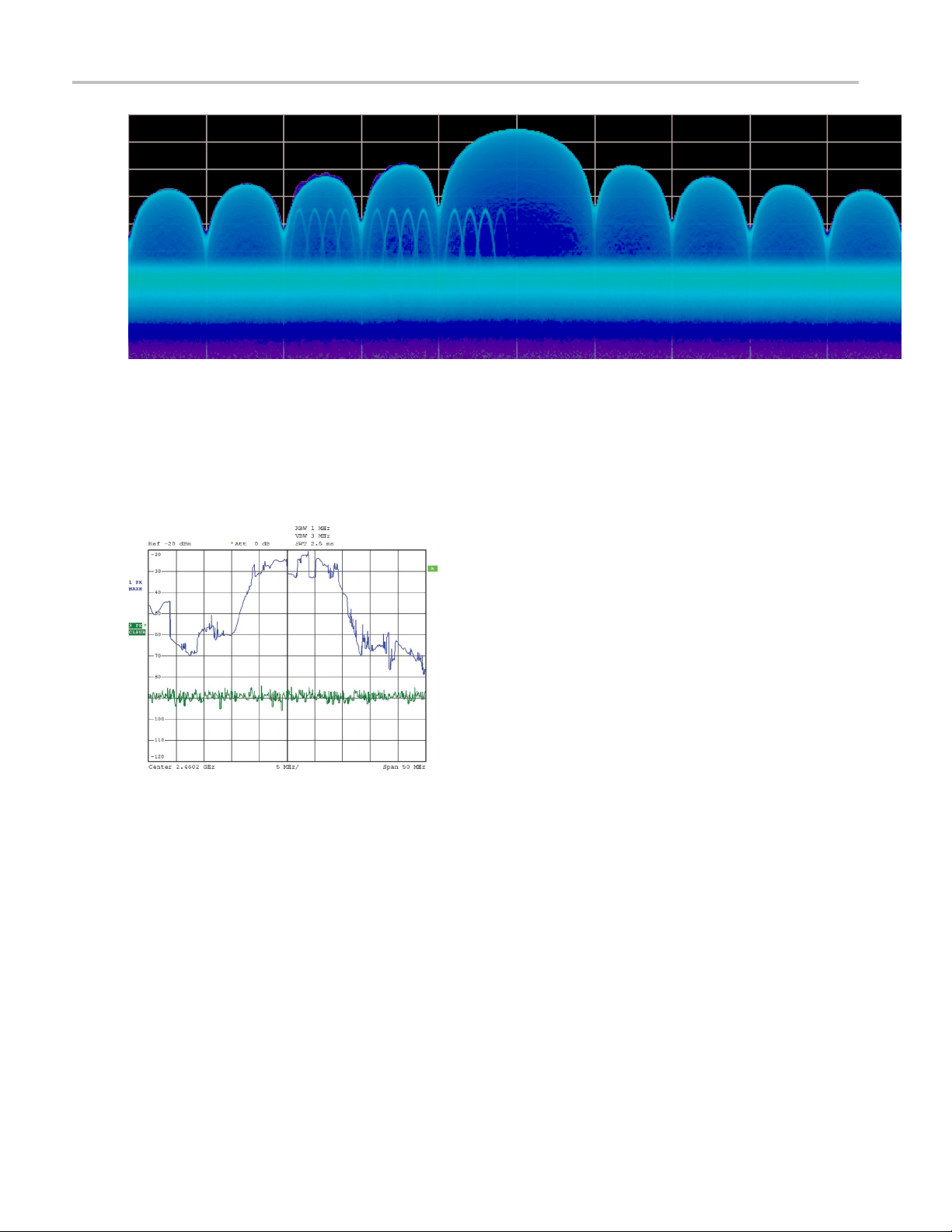
General Signal Viewing DPX Primer

Figure 1

Compare the display of a traditional swept spectrum analyzer (Figure 2) and that of a real-time spectrum analyzer with a DPX display (Figure 3). The signal captured is a typical WLAN interchange between a nearby PC and a more-distant network access point (AP). The laptop signal is nearly 30 dB stronger than the AP's signal because it is closer to the measuring antenna.

Figure 2

40 RSA6000 Series & RSA5000 Series Printable Online Help

General Signal Viewing DPX Primer

Figure 3

The traditional swept spectrum analyzer display, Figure 2, uses line traces that can show only one level for each frequency point, representing the largest, the smallest or the average power. After many sweeps, the Max Hold trace shows a rough envelope of the stronger laptop signal. +Peak detection was selected for the other trace in an attempt to capture the weaker but more frequent AP signal, but the bursts are very brief, so the likelihood of seeing one in any particular sweep is small. It will also take a long time to statistically capture

the entire spectrum of a bursted signal due to the architecture of the swept spectrum analysis.

The D PX display, Figure 3, reveals much more insight on the same signal. Since it is a bitmap image

d of a line trace, you can distinguish many different signals occurring within each update period

instea and/or different version of the same signal varying over time. The heavy band running straight across the lower third of the graph is the noise background when neither the laptop nor the AP is transmitting. The red lump of energy in the middle is the ON shape of the AP signal. Finally, the more delicate spectrum above the others is the laptop transmissions. In the color scheme used for this demonstration (“Temperature”), the hot red color indicates a signal that is much more frequent than signals shown in cooler colors. The

op signal, in yellow, green and blue, has higher amplitude but doesn't occur nearly as often as the AP

lapt transmissions because the laptop was downloading a ﬁle when this screen capture was taken.

How DPX Works

This section explains how DPX displays are created. The input RF signal is conditioned and down-converted as usual for a spectrum analyzer, then digitized. The digitized data is sent through an FPGA that computes very fast spectral transforms, and the resulting frequency-domain waveforms are rasterized to create the bitmaps.

The DPX bitmap that you see on screen is composed of pixels representing x, y, and z values for frequency, amplitude, and hit count (instruments with Option 200 provide Density as the z-axis value in place of hit count). A multi-stage process, shown in Figures 4a - 4d, creates this bitmap, starting with analog-to-digital conversion of the input signal.

RSA6000 Series & RSA5000 Series Printable Online Help 41

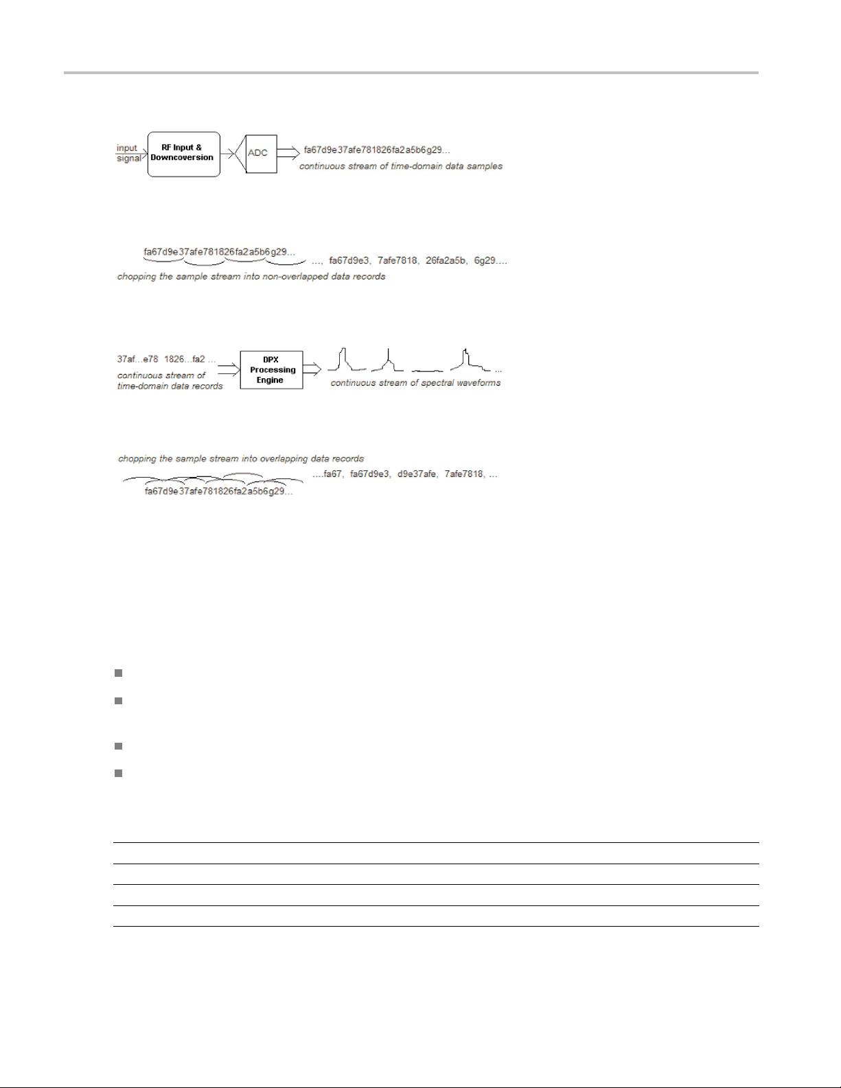
General Signal Viewing DPX Primer

Simpliﬁed Flow of Multi-stage Processing from RF Input Through to Spectrum Processing:

Figure 4a. RF signals are downconverted and sampled into a continuous data stream.

Figure 4b. Samples are segmented into data records for FFT processing based on the selected resolution bandwidth.

Figure 4c. Data records are processed in the DPX transform engine

Figure 4d. Overlapping the FFTs shortens the minimum event duration required for 100% probability of intercept.

Collecting spectral data. Sampling and digitization is continuous. The digitized data stream is chopped into

data records whose length is based on the desired resolution bandwidth (RBW). An additional requirement is placed on FFT length by the desired number of points in a trace (Option 200 only). Table 1 shows thi

s relationship and the FFT length is reported in the display if desired. Then the DPX transform engine performs a discrete Fourier transform on each record, continually producing spectral waveforms.

RF signals are downconverted and sampled into a continuous data stream.

Samples are segmented into data records for FFT processing based on the selected resolution bandwidth.

Data records are processed in the DPX transform engine.

Overlapped processing is used to improve minimum event duration performance.

Table 1: Minimum FFT length versus trace length (independent of span and RBW), Option 200

Trace length (points) Minimum FFT length

801 1,024

2,401 4,096

4,001 8,192

10,401 16,384

xxx

42 RSA6000 Series & RSA5000 Series Printable Online Help

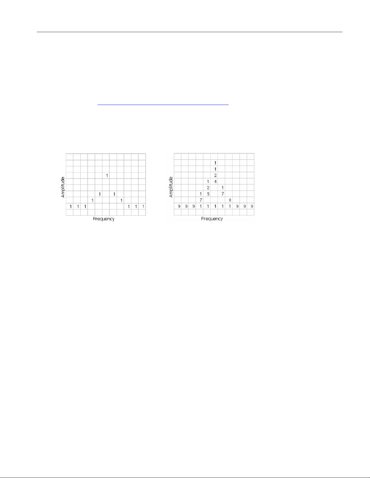
General Signal Viewing DPX Primer

As long as spectral transforms are performed faster than the acquisition data records arrive, the transforms can overlap each other in time, so no events are missed in between. Minimum event length for guaranteed capture depen consecutive data records in order for its amplitude to be accurately measured. Shorter events are detected and visible on screen, but may be attenuated. The DPX S pectrum RBW setting determines the data record length; narrow RBW ﬁlters have a longer time constant than wide RBW ﬁlters. This longer time constant requires longer FFTs, reducing the transform rate. Additional detail on minimum signal duration is provided in Guaranteed Capture of Fast Events

The spectral waveforms are plotted onto a grid of counting cells called the “bitmap database”. The number held by each database cell is the z-axis count. For simplicity, the small example grid used here in Figure 6 is 11x10, so our spectral waveforms will eac value for each (x) frequency. As waveforms are plotted to the grid, the cells increment their values each time they receive a waveform point.

ds on the length of the data records being transformed. An event must last through two

(see page 48).

h contain 11 points. A waveform contains one (y) amplitude

Figure 5. Example 3-D Bitmap Database after 1 (left) and 9 (right) updates. Note that each column contains the same total number of “hits”.

The grid on the left shows what the database cells might contain after a single spectrum is plotted into it. Blank cells contain the value zero, meaning that no points from a spectrum have fallen into them yet.

The grid on the right shows values that our simpliﬁed database might contain after an additional eight spectral transforms have been performed and their results stored in the cells. One of the nine spectrums happened to be computed as a time during which the signal was absent, as you can see by the string of “1” occurrence counts at the noise ﬂoor.

Frame updates. The maximum rate for performing the variable-length frequency tra ns forms that produce

those waveforms can be greater than 292,000 per second. Measurement settings that slow this transform rate include narrowing the RBW and increasing the number of points for the line traces available in the DPX display along with the bitmap. Even at their slowest, spectral transforms are performed orders of magnitude faster than a physical display can respond, and also too fast for humans to see, so there's no need to update the screen or measurements at this rate. Instead, the grid collects thousands of waveforms into “frames”, each covering about 50 milliseconds (ms). A 50 ms frame contains the counts from up to 14,600 waveforms. After each frame's waveforms have been mapped into the grid, the cell occurrence counts are converted to colors and written to the DPX bitmap, resulting in a bitmap update rate of around 20 per second.

Frame length sets the time resolution for DPX measurements. If the bitmap shows that a -10 dBm signal at 72.3 MHz was present for 10% of one frame's duration (5 ms out of 50 ms), it isn't possible to determine just from the DPX display whether the actual signal contained a single 5 ms pulse, one hundred

RSA6000 Series & RSA5000 Series Printable Online Help 43

General Signal Viewing DPX Primer

50 microsecond (μs) pulses, or something in between. For this information, you need to examine the spectral details of the signal or use another display with ﬁner time resolution, such as Frequency vs. Time or Amplit

ude vs. Time.

Converting occurrence counts to color. About 20 times per second, the grid values are transferred to the

next process step, in which the z-axis values are mapped to pixel colors in the visible bitmap, turning data into information (Figure 6). In this example, warmer colors (red, orange, yellow) indicate more occurrences. The color palette is user-selectable, but for now we will assume the def

ault “temperature”

palette.

Number of Occurrences Color

0black

1blue

2 light blue

4 green blue

6 yellow

8 red orange

9red

Figure 6. Example Color-mapping algorithm

xxx

cyan

green

orange

The result of coloring the database cells, Figure 7, according to the number of times they were written into by the nine spectrums, one per pixel on the screen, creates the DPX displays.

Figure 7. Color-coded low-resolution example (left) and a real DPX display (right).

In addition to the choice of palette, there are z-axis scaling adjustments for Maximum, Minimum, and Curve. Maximum sets the occurrence value that will be mapped to the highest color in the palette. Minimum sets the occurrence value for the lowest color. In the “temperature” palette, the highest color is deep red and the lowest is dark blue. Occurrence values less than the selected Minimum are represented

44 RSA6000 Series & RSA5000 Series Printable Online Help

General Signal Viewing DPX Primer

with black pixels, while pixels that exceed the selected Maximum are red in hue but somewhat transparent. Values between Maximum and Minimum are represented by the other colors of the palette.

Adjusting the Minimum above the black default allows you to concentrate most of your color resolution over a small range of medium or higher occurrence rates to visually discriminate between different signals that have nearly equal probability values.

To see why adjustable color scaling is useful compare Figures 8 and 9. On the Scale tab, the Max control is set to 100% in Figure 8. The range of colors now covers the full z-axis range of densities from 0 to 100%. The signals used to create this bitmap are fairly diffused in both frequency and amplitude, so most pixels have low occurrence counts or density values and the upper half of the color palette is unused.

Figure 8. DPX spectrum bitmap with default color scale settings.

When the Auto Color button is selected, the Maximum control's value is set to the highest pixel value in the current bitmap, shown in Figure 9. Now none of the available colors remain unused. The entire palette is mapped to the occurrence values present at the time the button is selected, providing better visual resolution for low densities. Selecting the Autoscale button in the DPX display scales all three axes based on current results.

Figure 9. The Auto Color function optimizes the color scale settings.

Color Mapping Curves

The mapping between z-axis values and color does not have to be linear. The Curve control lets you choose the shape of the mapping equation. A Curve setting of 1 selects the straight-line relationship.

RSA6000 Series & RSA5000 Series Printable Online Help 45

General Signal Viewing DPX Primer

Higher Curve numbers pull the curve upwards and to the left, concentrating color resolution on lower densities. Settings less than 1 invert the curve, moving the focus of the color range towards higher density values. Figur

e 10 shows the mapping curves.

Figure 10. Representative color mapping curves for the “Temperature” palette.

Using the same signal shown in Figures 8 and 9, the impact of the Curve control can be observed. With the Curve control set to 1 in the Scale tab, shown in Figure 11, the mapping between color and density is linear, so the colors spread evenly across the full density range. The color distribution is visible in the colored palette illustration to the left of the Curve control in the Settings panel.

Figure 11. Over a narrow Signal Density range, the color curve is set to 1.

When the Curve control is set to 0.5, as shown in Figure 12, the best color resolution is in the upper half of the density range, and only the dark blues are assigned to densities below 50%. Note the difference in the palette illustration.

46 RSA6000 Series & RSA5000 Series Printable Online Help

General Signal Viewing DPX Primer

Figure 12. Ad density range.

In Figure 13, the Curve control is increased to 3. The majority of colors shifts to the lower half of the density scale, but various shades of orange and red are still available for densities above 50%.

Figure 13. For color curve settings greater than 1, better contrast is provided for events near the low end of the density range.

justing to values less than 1, increases the contrast for viewing events in the top half of the selected

Swept DPX

DPX Spectrum is not limited in span by its real-time bandwidth. Like the regular Spectrum display, DPX Spectrum steps through multiple real-time frequency segments, building a wide-span display with line traces and the bitmap (Option 200 only). See Figure 14.

Figure 14. Off-air ambient signals over a 1 GHz span in the swept DPX display.

The analyzer “dwells” in each frequency segment for one or more DPX frames, each containing the results of up to 14,600 spectral transforms. Dwell time is adjustable, so you can monitor each segment of the sweep for up to 100 seconds before moving to the next step. While dwelling in a segment, the probability

RSA6000 Series & RSA5000 Series Printable Online Help 47

General Signal Viewing DPX Primer

of intercept for signals within that frequency band is the same as in normal, real-time spans: 100% capture of events as short as 10.3 μsec.

A full pixel bitmap is created for every segment and compressed horizontally to the number of columns needed for displaying the frequency segment. Compression is done by averaging pixel densities of the points being combined together. The ﬁnal swept bitmap contains a representation of the same pixel bitmap resolution, just like the non-swept bitmaps. Line traces are also created in full for each segment, and then horizontally compressed to the user-selected number of trace points for the full span.

A complex algorithm f implemented. The variables in the equation include user-adjustable control settings like Span, RBW, and number of trace points, RF and IF optimization, and Acquisition BW. Installed hardware options also can affect the span segmentation. The number of segments ranges from 10 to 50 for each 1 GHz in a sweep.

A helpful piece of information for operators is the actual Acquisition Bandwidth used for capturing each segment. “Acq BW” is shown in the Acquire control panel on the Sampling Parameters tab. Acq BW is typically set automatically by the instrument, based on the needs of all the open displays, but can also be set manually. In either case, the displayed bandwidth is used for every frequency segment in the swept DPX display, though in practice, the displayed portion of the segment is somewhat narrower than the actual Acquisition BW, for performance reasons.

The entire instrument frequency range of many GHz can be covered in a DPX sweep. The Dwell Time control sets the amount o set between 50 ms and 100 seconds.

Figure 15. During swept DPX operation, t segment used to construct the composite DPX display.

or determining the number and width of each frequency segment has been

f time DPX spends in each segment. This control, circled in Figure 15, can be

he Dwell time control adjusts the observation time of each frequency

Guaranteed Capture of Fast Events

The main reason that swept-tuned and step-tuned spectrum analyzers can't provide 100% Probability of Intercept, POI, for a signal that isn't continuously present is that they spend only a short period of time tuned to each segment of their frequency span during each sweep. If something happens in any part of the span other than where it is tuned at that instant, that event will not be detected or displayed. There is also a period of time between sweeps, retrace time, during which the analyzer is not paying attention to the input signal. FFT-based analyzers, including vector signal analyzers, also miss signals during the time between acquisitions. Their POI depends on a combination of factors including span, number of FFT points, acquisition time, memory read/write time, and signal processing speed. Vector analyzers process information sequentially, so when read/write from data and processing is occurring, data is not being acquired.

RSAs, on the other hand, capture data across all frequencies within their real-time span during every acquisition. With Tektronix' exclusive Frequency Mask trigger and DPX Density trigger, POI increases to

48 RSA6000 Series & RSA5000 Series Printable Online Help

General Signal Viewing DPX Primer

100%, insuring capture of any spectral event matching the trigger deﬁnition. When operating in free run as a simple spectrum analyzer, the RSA has a POI similar to other FFT-based analyzers, with gaps between each acquisit

ion. Processing is done concurrent with the acquisitions.

Guaranteed Capture in DPX Real-Time Spans

The DPX display captures any signal that is at least 10.3 microseconds long (for instruments with Option

200) and within the real-time bandwidth. This performance is possible because the RSA computes up to 292,000 spectrum transforms per second. The faster the spectrum updates, the shorter the time between acquisitions and the greater the probability that any signal will be detected.

Table 1 shows the speciﬁed minimum signal duration (MSD) for 100% probability of intercept under various combinations of Span and RBW in DPX for a representative RSA model. As you can see, MSD is affected by multiple factors.

Table 2: Minimum signal duration speciﬁcations for RSA6000 series spectrum analyzers

Span

(MHz)

110 1000 110 1024 292,969 10.3

110 300 367 2048 146,484 20.5

110 100 1100 4096 73,242 41.0

110 30 3667 16384 18,311 163.9

110 20 5500 32768 9,155 327.7

xxx

Options 110 and 200 under various combinations of control parameters.

With

RBW (kHz)

Span/RBW

Ratio

FFT

Length Spectru

m/sec

100% POI

MSD for

(μs)

To demonstrate the POI in action, a challenging bi-stable signal is used. A CW sinusoid sits at 2.4453 GHz

of the time, but every 1.28 seconds, its frequency changes for about 100 μs before returning to

most normal. The duty factor of this transient is less than 0.01%.

ure 16 shows a swept analyzer set up for a 5-second sweep of its MaxHold trace. It shows that there is

Fig something occurring around the signal. This sweep rate was empirically determined to be the optimum rate for reliable capture of this signal in the shortest time. Faster sweep times can reduce the probability of intercept and result in fewer intersections of the sweep with the signal transient.

RSA6000 Series & RSA5000 Series Printable Online Help 49

General Signal Viewing DPX Primer

Figure 16. Swept spectrum display of the infrequent transient.

The DPX display shown in F lot more information can be discovered about the transient. It is obvious at ﬁrst glance that the signal is hopping by about 3 MHz, with 1.2 MHz of frequency overshoot on transitions

Figure 17. The DPX spectrum display after 5 seconds. The MaxHold trace is cyan.

igure 17 shows the exact same event, also captured over a 5 second period. A

Guaranteed Capture in DPX Swept Spans

Probability of intercept (POI) for signals within a single segment, while DPX is dwelling in that segment, is the same as for non-swept DPX operation (POI = 100% for events as brief as 10.3 microseconds). But just as in traditional swept analyzers, during the time the acquisition is tuned to any one segment, the analyzer is not monitoring signals in any of the other segments, so probability of capture in segments

50 RSA6000 Series & RSA5000 Series Printable Online Help

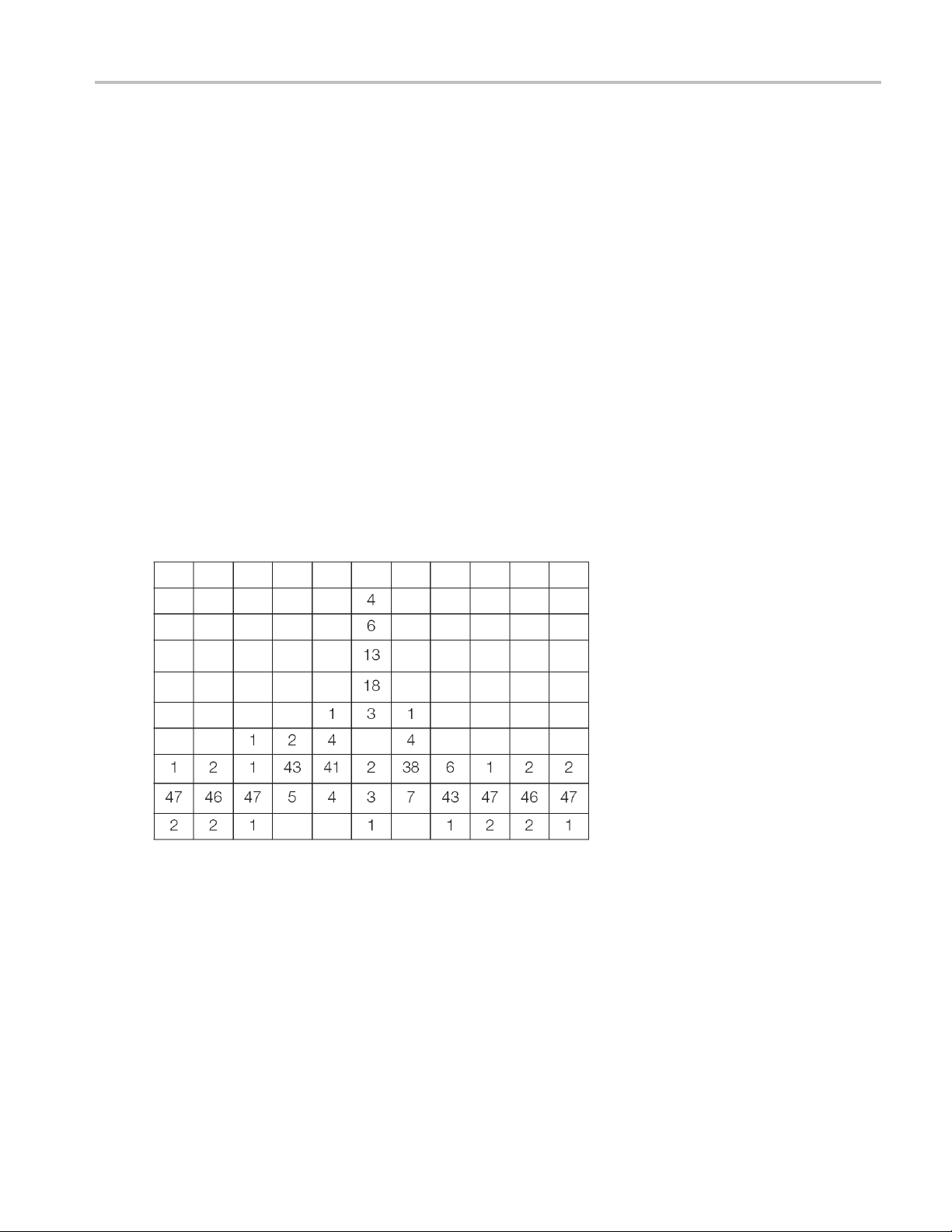
General Signal Viewing DPX Primer

other than the current one is zero. Because of the wide real-time bandwidth, the number of segments needed to cover the span is much less than for swept analyzers, so the overall probability of intercept is signiﬁcantly

Another factor affecting POI is number of trace points. The bitmap is always 801 points wide, but the line traces a 4001, and 10401. Frequency transforms for traces containing more than 801 points take longer, and this lower waveform update rate increases the minimum signal duration proportionally. This caution applies for swept and non-swept operation. The trace length control is on the Prefs tab in the DPX control panel.

better for DPX sweeps.

llow user selection for number of points. 801 is the default and the other choices are 2401,

DPX Density Measurements

“Density” is a measure of the amount of time during a deﬁned measurement period during which signals are present within a particular area of the DPX Spectrum bitmap. A clean CW tone gives a 100% reading, whileapu how density is computed from hit counts.

lse that is on for one microsecond out of every millisecond reads 0.1%. This section describes

If we plo we already plotted), each column ends with a total of 50 hits (Figure 18). The density for any one cell in a column is its own count value divided by 50, expressed in percent as shown in Figure 19. The math is very simple: a cell with 24 counts has a 48% density. In practice, instead of batches of 50 waveforms, we collect a frame of thousands of waveforms before each update to the density bitmap.

Figure 18. Grid showing cell counts after 50 waveforms. For each column, the sum of z-axis values is 50.

t 41 more waveforms into the example grid we used previously in Figure 6 (in addition to the nine

RSA6000 Series & RSA5000 Series Printable Online Help 51

General Signal Viewing DPX Primer

Figure 19. Grid after converting occurrence counts to percent density values. The sums of the cell density measurements within each column are all 100%.

Measuri

Hit counts are cleared after every frame update, as long as Persistence is not turned on. The density value fo Markers can be used to see the Density value for one or more individual points on the screen, enabling measurements of the signal density at any interesting point in the DPX display.

In Figure 20, Wireless LAN signals are analyzed in the presence of a Bluetooth radio signal in the 2.4 GHz ISM band.

Figure 20. DPX display of WLAN and Bluetooth signals, with a marker on the highest signal.

ng Density with Markers

r any pixel is simply the percent of time it was occupied during the most recent 50 ms frame.

The “Marker to Peak” function was used to ﬁnd the peak signa l recorded in the display. The marker readout in the upper left corner of Figure 20 shows the Density, Amplitude, and Frequency for the pixel you selected with the marker. By adding additional markers, you can measure the signal density differences between multiple signals of interest.

52 RSA6000 Series & RSA5000 Series Printable Online Help

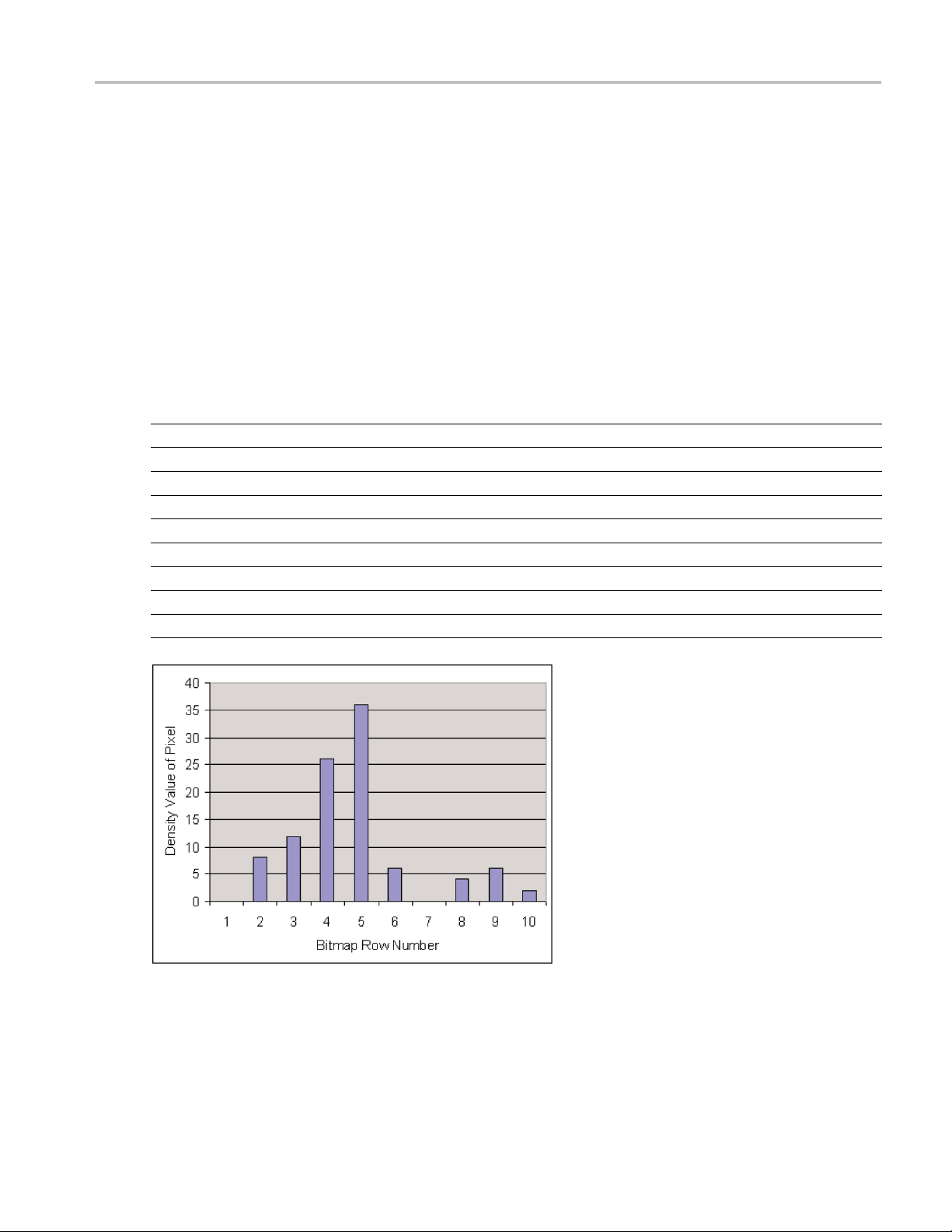
General Signal Viewing DPX Primer

Marker Peak Search in the DPX Bitmap

Markers on the DPX bitmap can search for peaks, similar to marker peak searching on spectrum line traces. For a human, it is pretty easy to discern “signals” in the bitmap picture. Your brain intuitively identiﬁes strings of contiguous bright pixels. This isn't so easy for a computer. The ﬁrst thing the RSA must do for an through these density peaks for the amplitude peaks you want to ﬁnd.

y peak search is analyze pixel density values to identify apparent signals. Then it can sift

Z-axis dens

ity values for the pixels in each column of the bitmap are internally converted into histograms to ﬁ nd density peaks indicating the presence of signals. Table 2 shows the ﬁve middle columns from the example grid we used to illustrate density measurements in a previous section (Figure 19). The density values for each pixel in the middle, highlighted column are plotted on the y axis in the bar chart in Figure 21. The bar chart x axis is bitmap row number, numbering from the top of the table.

Table 3: Bitmap section showing density values.

0% 0% 0% 0% 0%

0% 0% 8% 0% 0%

0% 0% 12% 0% 0%

0% 0% 26% 0% 0%

0% 0% 36% 0% 0%

0% 2% 6% 2% 0%

4% 8% 0% 8% 0%

86% 82% 4% 76% 12%

10% 8% 6% 14% 86%

0% 0% 2% 0% 2%

xxx

Figure 21. Bar chart of the density values in the bolded column of Table 2.

Assume that Density Threshold is s et to 5% and Density Excursion to 5% also. Starting with x=1 in the bar chart, test each bar against the threshold. The threshold criteria is met at x=2. Keep testing until you

RSA6000 Series & RSA5000 Series Printable Online Help 53

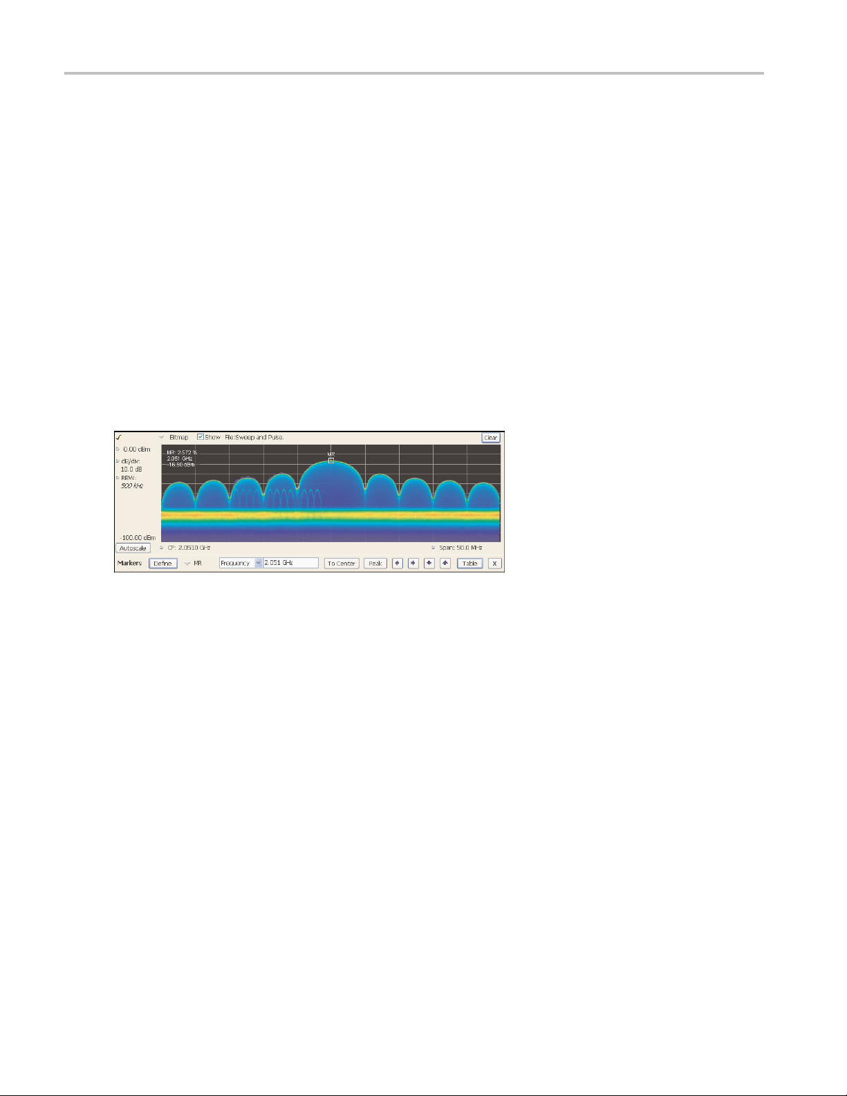
General Signal Viewing DPX Primer

ﬁnd a bar that is shorter than the previous bar by at least the Excursion setting. In this case it is x=6. This tells us that a “signal” covers rows 2 through 5. Its density peak is at row 5.

Now you can look for another peak. Continue looking at bars to the right and you will ﬁnd a density value at row 9 that meets the threshold criteria, but since there are no bars to the right of it that meet the excursion cr had1%density,thenrow9wouldbeadensitypeak.

iteria, we can't declare row 9 a signal because it fails to meet the excursion criteria. If row 1

Once densit When the Peak button is selected, the analyzer checks the histograms of every column in the bitmap and ﬁnds the density peak with the highest amplitude. The amplitude search has its own versions of Threshold and Excursion settings, but in dBm and dB units. When Next Peak Down command is given, the search will scan inside the current column for the next density peak. Next Peak Right examines each column to the right of the current marker location to locate density peaks that also meet the amplitude peak criteria.

To demonstrate the value of marker peak search in the DPX bitmap, we will use the time-multiplexed signals showing multiple amplitude levels from an example earlier in this manual. The Peak button and its m density peak of highest amplitude in the bitmap.

Figure 22. The marker was positioned by selecting the Peak button. Density, frequency, and amplitude measurements at the marker are displayed in the upper left corner of the graph.

y peaks are found for all columns in the bitmap, we can start looking for the amplitude peaks.

enu equivalent place the active marker on the peak signal in Figure 22. The peak signal is the

The Marker Toolbar, at the bottom of Figure 22, allows easy navigation of peak signals (Peak Left, Peak Right, Next Peak Up,orNext Peak Down). Selecting the arrow keys enables the marker to search for amplitude/density peaks at other frequencies, while the Next Peak Up and Next Peak Down arrows

nable the marker to search for other high-density points at the same frequency.

In the Deﬁne Peaks tab of the Deﬁne Markers control panel, Figure 24, you can adjust the density threshold

nd excursion controls to modify search behavior. The amplitude threshold and excursion controls also

a apply to DPX marker searches. Smoothing keeps the marker from ﬁnding multiple peaks within the same apparent signal by averaging an adjustable number of pixel densities together, but it does not affect the single-pixel measurement readout displayed by the marker.

54 RSA6000 Series & RSA5000 Series Printable Online Help

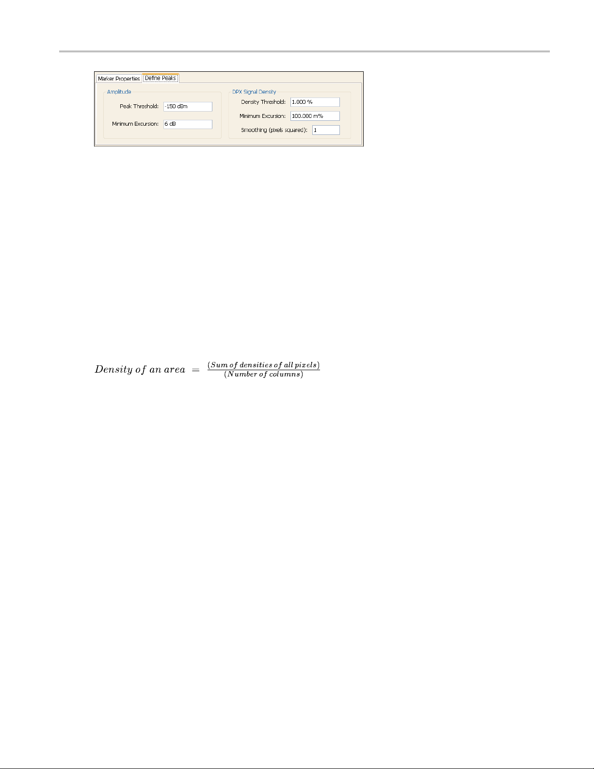
General Signal Viewing DPX Primer

Figure 24. Amplitude and Signal Density controls can be adjusted to deﬁne Peak search behavior.

Density Measurements over an Adjustable Area (“The Box”)

The density for a single pixel is its ratio of actual hits vs. possible hits over a deﬁned time period, and markers display these density values. For mea suring density over an area larger than one pixel, Option 20 mouse or ﬁnger.

0 includes a measurement box you can resize and drag around in the DPX display with your

If you co density of this area would be the sum of the included pixels' density values. For example, if the box was three pixels tall and the density values for these pixels were 4, 2, and 7% respectively, the overall density for the three-pixel area would be 13%. Imagine a box one pixel wide and as tall as the graph. Assume that the input signal's amplitude was such that all hits fell at or near the vertical center of the screen. Since 100% of the waveforms written to the bitmap passed through the box, the density for the box is 100%.

When you widen the box to cover a broader range of frequencies, software computes the density sum for the included pixels in each column inside the box. The aggregate density value for this box i s the average den result, there must not be any hits above the top edge of the box or below its bottom edge. In other words, every waveform drawn across the graph entered the box through its left side and exited the box through its right side, with no excursions out the top or bottom. Figure 24 demonstrates this principle on a CW signal. As you can see on the left-hand side, no amplitudes exist above or below the box; the density of the signal is 100%. On the right hand side, there are signals below the box, therefore the density is less than 100%.

uld make the box so narrow that it contained only points within a single column of pixels, the

sity, calculated by adding the column density sums then dividing by the number of columns. For a 100%

RSA6000 Series & RSA5000 Series Printable Online Help 55

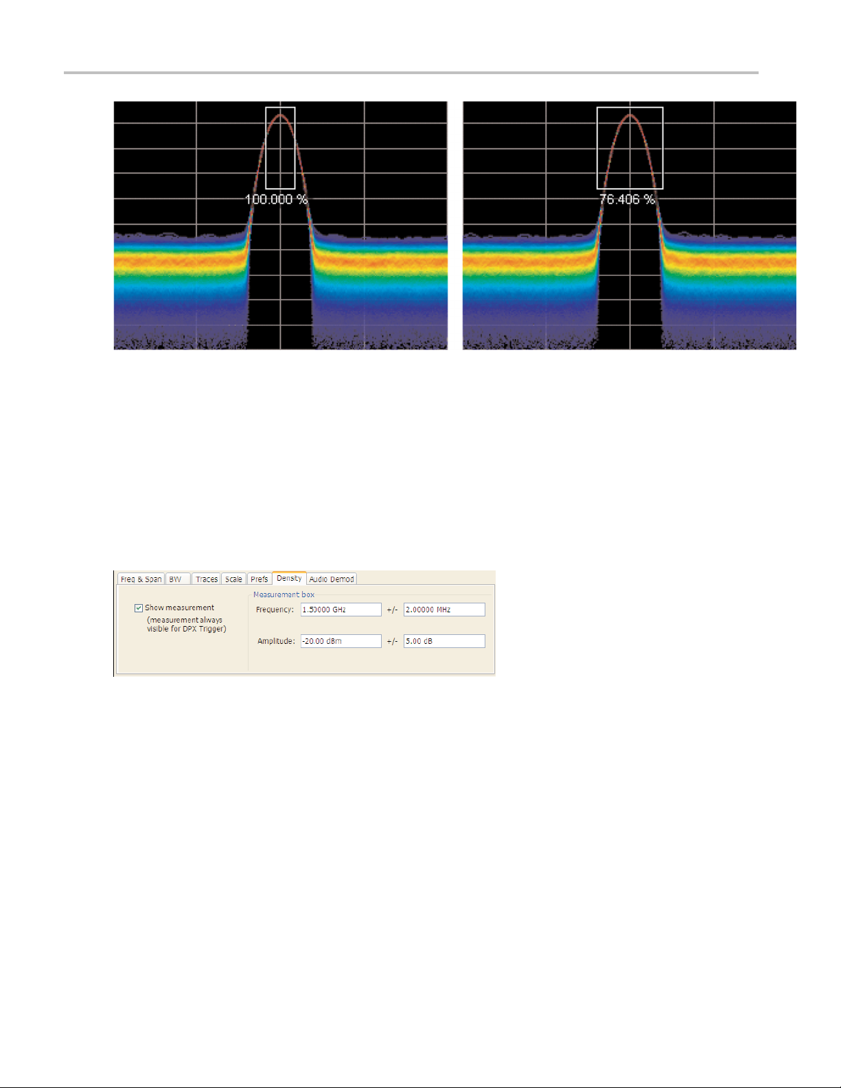
General Signal Viewing DPX Primer

Figure 24. Density of signals deﬁned within an area. Left: Correct measurement of a CW signal. All columns in the box inclu expected. Some columns in the box contain no hits, so they contribute zeros to the calculation of average density.

The density measurement box' vertical size and location are always set in dB and dBm, no matter what units you have selected for measurements. (Amplitude control panel > Units tab) The box is not draggable when the selected units are linear (such as Amps, Volts, Watts…), though you can still adjust its size and location using the Frequency and Amplitude controls in both the DPX Settings > Density and Trigger > Event tabs. Since the vertical scale is non-linear, a box of constant amplitude changes visual height as it chang

de the signal. Right: Incorrect measurement area. The measurement is accurate, but probably not what you

es vertical position, a disconcerting effect if you are trying to drag it.

Figure 25. DPX Density control panel is used to deﬁne the area of interest for DPX density measurements.

A readout will appear somewhere in the graph. If the box is off-screen, the readout will be accompanied by an arrow pointing towards the invisible box. Grab this readout with your mouse or ﬁnger and drag the density readout to the area you want to measure.

To adjust the box size, a mouse is the easiest way to drag the sides and corners of the rectangle. For precise settings, use the knob, arrow keys, or keyboard to adjust frequency and amplitude values for the rectangle. These controls are located in the right half of the Density tab in the control panel.

Persistence

Previous sections of this topic have assumed that persistence was not applied to the DPX bitmap. Without persistence, hit counts in the grid are cleared after each frame update. Now we will describe how

56 RSA6000 Series & RSA5000 Series Printable Online Help

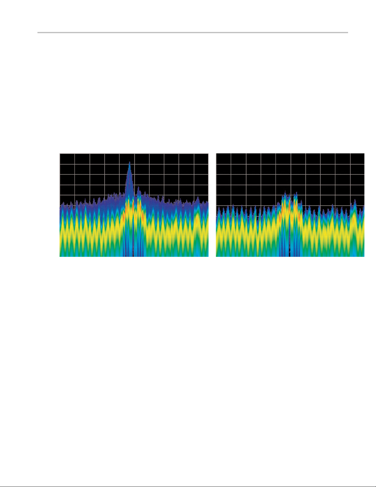
General Signal Viewing DPX Primer

persistence modiﬁes this behavior, starting with inﬁnite persistence because it is simpler than variable persistence.

Hit counts are not cleared between frames if inﬁnite persistence is enabled. When the instrument is set up for continuous acquisitions, hits keep collecting until you stop acquisitions or click the Clear button above the DPX display. Software keeps track of the total number of waveforms computed during the entire collection period. Density equals the total number of hits to a cell divided by the total number of waveforms.

Variable persistence is trickier. A single-occurrence signal shown in the bitmap does not disappear suddenly upon the next frame update, nor does it linger forever. It fades gradually away. The user sets a time constant for the Dot Persistence control which determines how long it takes for signals to fade. Fading is accomplished by reducing the hit count in every cell, after each frame update, by a factor based on the persistence time constant. The longer the time constant, the less the hit counts are reduced.

Figure 26. Example of fast transient discovery with and without variable persistence turned on. In the display on the left, with variable persistence of 10 seconds, the occasional sub-second transient that spikes up above the normal signals is held in the display rather than disappearing as soon as the signal goes away. The display on the right, with persistence turned off, requires watching the display continually to see the brief signal.

Not only are single-occurrence signals allowed to remain in the display for awhile by variable persistence, additional hits keep piling on. The result is that cell values are no longer pure hit counts; they include counts due to new hits from waveforms plus proportionally reduced counts from prior frames. As part of translating hit counts into density values, a new software algorithm uses a ﬁnite-series equation to discriminate between the effects of persistence and the arrival of new hits. The inﬂationary effects of persistence on cell counts are removed, so density readings represent the true ratio of actual hits to possible hits over the persistence interval.

The density computation for variable persistence is a very good estimate of true signal density, with errors of less than 0.01%. For exact density measurements, use either no persistence or inﬁnite persistence.

Another subtlety of persistence is its smoothing effect on the density measurement of intermittent signals. Consider a pulse that is on for 10 m s and off for 90 ms of each 100-ms cycle. We'll make the simplifying assumption that the pulse ON time always falls entirely within a single DPX frame update (50 ms). If persistence is not applied, the density measurement is computed on each individual frame. The results will be 20% for each frame containing the ON time and 0% for the other frames. If inﬁnite persistence

RSA6000 Series & RSA5000 Series Printable Online Help 57

General Signal Viewing DPX Primer

is enabled, however, the density measurement will settle to 10% after the second frame, and remain at this value for as long as the pulsing continues. With persistence, the density is effectively computed over many fram

es.

Persistence Effects on Density

Persistence does not alter colors in a density-based bitmap. Its effect is to extend the amount of time over which densities are calculated, leaving signal events visible for the persistence duration.

Before the introduction of density measurements and extra-long hit counters, persistence caused colors to “bloom”, becoming more and more intense over time as the hit counts increased. Longer persistence intervals caused increased blooming, turning crisp signals into fat red stripes. When hit counts are converted to density values (requires Option 200), the display is not subject to this effect. As long as the input signals maintain reasonably stable repetition rates and duty ratios, their density values will also remain st

If you are accustomed to the original hit-count-based persistence displays, it may seem counterintuitive that rep persistence. A quick review of the density algorithm explains why: the hit count is divided by the total number of waveforms over the persistence interval. For example, if a signal occupies a pixel 50% of the time over a period of 15 minutes, the density reading will be 50% throughout the entire 15 minutes, though the underlying hit count is steadily increasing.

able despite ever-increasing hit counts in the underlying grid cells.

eating signals in a density-based bitmap will not get brighter and redder over time with inﬁnite

is Resolution

Z-Ax

Another factor that can cause color bloom is overﬂow of the hit counters. If a pixel could only count up to

0 hits, its density and color values would clip at 100% after just 1000 hits, even if waveform points

100 continue to arrive in the same pixel location. With waveform points being written to the bitmap at rates approaching 300k/sec, counts add up really fast for highly-repetitive signals. Deeper counters permit higher hit counts, so overﬂow happens much later, as shown in Table 3.

Table 4: Comparison of DPX z-axis resolution and its effect on saturation.

RSA6000 Series Standard R SA6000 Series Option 200

Hit Count

Maximum Hit Count

Minimum Time until Overﬂow (for pixels with 100% density)

xxx

16-bit integer

<50 msec 8.1 hours

36-bit custom ﬂoat (equivalent to 33-bit integer)

Clipping due to overﬂow of the counters in one or more cells will not occur until hours have passed, or even days.

Onemorebeneﬁt to having deeper hit counters is better visual resolution of density. RSAs with the highest-performance DPX hardware installed use ﬂoating-point numbers to count hits, allowing us to count billions of waveforms while retaining one-hit resolution, providing better than 99 dB of dynamic range for density measurements. Density measurements in μ%, n%, and even f% ranges are quite possible for extremely rare signals ca ptured with inﬁnite persistence.

58 RSA6000 Series & RSA5000 Series Printable Online Help

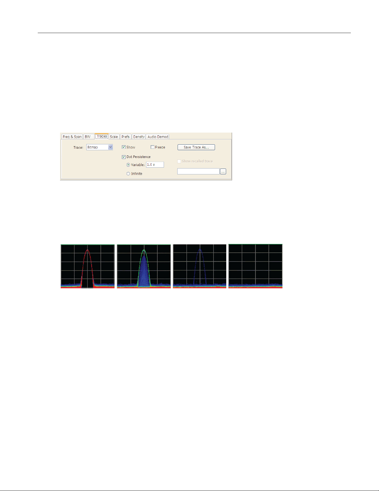
General Signal Viewing DPX Primer

With straight-line mapping between density and color (Curve setting o f 1), resolution is ﬁxed by the number of colors in the palette. For non-linear mappings (Curve settings higher or lower than 1), most of the colors a discriminate ﬁner differences between density values in that range.

re concentrated at either the low or high end of the density scale, so you can visually

Persistence Adjustments

Dot Persistence can be enabled for the “Bitmap” trace using the Settings control panel. The Persistence can be displayed as Inﬁnite or Variable. For Variable Persistence, you can select the time constant for fading in seconds as shown in Figure 27.

Figure 27. The trace settings control panel allows user control of persistence p

Figure 28 demonstrates the observed behavior of variable persistence when a CW signal, represented in the ﬁrst frame, is turned off. Even if the event was instantaneous and was conﬁned within a single frame, you will observe the color changing to indicate lower and lower density values, until the signal ﬁnally disappears entirely.

Figure 28. With variable persistence, a brief CW signal captured by DPX remains in the display for an adjustable periodoftimebeforefadingaway.

arameters.

DPX Density Trigger

The standard DPX display shows you a clear picture of transients and other hard-to-ﬁnd signals. The version of DPX in the RSA6000 Option 200 goes well beyond helping you discover these difﬁcult to ﬁnd signals by actually triggering on their appearance to capture them into acquisition memory for in-depth analysis. If you can see it in the DPX bitmap, you can trigger on it.

Other trigger methods can detect signals that e amplitude-vs-frequency mask, but they can't ﬁnd a signal at a particular frequency if another signal of higher amplitude is sometimes present at that same frequency. The Runt trigger addresses some of these signal-under-signal cases, but not all. As shown in Figure 29, the DPX Density trigger can discriminate signals within a precise amplitude-frequency range without the operator having to know any characteristics of the target signal besides where it might show up in the DPX Spectrum graph.

RSA6000 Series & RSA5000 Series Printable Online Help 59

xceed an a mplitude threshold, or even a sophisticated

General Signal Viewing DPX Primer

Figure 29. Example of Density Trigger. Left: A free-run DPX display showing pulses with varying frequency. Occasionally, a short pulse in the middle appears for a split instant, but it is hard to capture it with just a Run/Stop button. Right: The triggered DPX displays shows the low-amplitude pulse that was not apparent in the untriggered display. The analyzer was set to trigger whenever the average density in the user-drawn box measured 50% or higher.

The DPX Density trigge r uses the same screen-based measurement box as the DPX Density measurement. While the box. When the target s ignal ﬁnally appears, the density value increases. The trigger system monitors the density measurement and activates a trigger whenever the density value exceeds the adjustable density threshold. The only thinking you have to do is to set this threshold to a level somewhere between the normal density readings and the density due to the trouble-making signal. However, the instrument software can compute the threshold value automatically.

target signal is absent, the density measurement characterizes the “normal” signals within the

Trigger On This™

igger On This™ function allows you to point and click to set up the DPX Density trigger. By

The Tr right-clicking on a spot within the DPX display, or pressing and holding your ﬁnger on the RSA6000 Series touchscreen display for about a second, a menu selection will appear. Selecting Trig ger On This causes a DPX Density box to appear and automatically adjusts the threshold. The DPX display will now only update whenever the a utomatic threshold is exceeded. Subsequently, if needed for your signal, open the Trigger control panel to adjust the density threshold or the size of the measurement box until

e event is reliably captured.

Automatic Threshold Adjustment by Trigger On This™

The trigger density threshold automatically set by Trigger On This is 80% of the measured value. If the signal was present at the moment you selected Trigger On This, the threshold will be 20% less than the signal density, so the next time the signal is present long enough (or present enough times) to exceed the threshold density, it will cause a trigger. If the signal happened to be missing when you selected Trigger On This, the threshold value will be even lower. If you clicked in a part of the display with no signal activity at all, the threshold will be set to zero. Any signal that shows up here will ﬁre the trigger, as shown in Figure 32.

60 RSA6000 Series & RSA5000 Series Printable Online Help

General Signal Viewing DPX Primer

Figure 30. The analyzer triggered when the density in the DPX measurement box exceeded the threshold set by Trigger On This. You can see in the Spectrogram and Frequency-vs-Time displays that the signal event which caused the trigger was a quick frequency hop. The Time Overview shows that the signal amplitude never changed, so a power level trigger would not have worked.

DPX Density Trigger Timing

The time resolution for DPX density measurements is the frame length, around 50 m s. A basic implementation of the DPX Density trigger concept is also frame-based, so a trigger event that occurs anywhere within a frame will not be recognized until the end of the frame. Therefore, the worst case trigger uncertainty is 50 ms.

DPX Density trigger doesn't always have to wait until the end of a frame before ﬁring. For the common conﬁguration of triggering when the measured density is higher than the threshold, the density measurement in the trigger can be computed many times within each frame and it can ﬁre the trigger

soon as the threshold is exceeded.

Consider the case where the threshold is zero. As soon as a single waveform causes a hit within the

easurement box, we know that the density is greater than zero. It takes a little longer to test for a 5 or

m 10% density, and even more time for thresholds at or near 100%.

The DPX Density trigger can also be set to ﬁre when the measured density is below the threshold value. This is useful when you suspect that your signal is missing some of the time. For a signal that is supposed to be CW, you can set the trigger controls to acquire when the density measurement of the signal peak drops below 100%. When using the “lower than” form of the DPX Density trigger, the time resolution is

RSA6000 Series & RSA5000 Series Printable Online Help 61

General Signal Viewing DPX Display Overview

one frame because of the following logic: We can't be sure the actual density is less than, say, 15% until at least 85% of the full test time has elapsed. In order to keep things simple and fast in the trigger module, the RSA just waits

until the end of each 50 ms frame to do the “lower than” comparisons.

Persistence and DPX Density Trigger

The smoothing effect of persistence on density measurements can help in determining a good threshold value. With persistence turned off, an infrequent signal's density reading jumps between higher and lower values as it turns on and off, and it can be hard to read these ﬂashing numbers. By turning persistence on, you instruct the instrument to average the density over a longer time period. This density result is somewhere between the ON and OFF density values - the very deﬁnition of a good trigger threshold.

Unlike the DPX Density measurement, the DPX Density trigger is not affected in any way by persistence. Density calculations in the trigger system are made with hit count data received from each individual DPX frame, be is avera ged over many frames due to persistence, the trigger is computing density for each frame and comparing these quick snapshots against the threshold setting.

fore any persistence is applied. Even when the density measurement reading in the display

DPX Display Overview

The DPX display enables you to see how traces change over time and thus displays signal events that cannot be seen on a swept spectrum analyzer. A DPX Spectrum indicates how traces change in two ways. First, it uses color shading to show how consistent the shape of a trace is. Second, it uses persistence to hold signals on the screen so you can see them longer.

DPX Display

The DPX display works by using a two-dimensional array to represent points on the display. Each time a trace writes to a point on the display, a counter in the array is incremented. A color is assigned to each point in the display based on the value of its counter. Thus, as acquisitions occur over time, a colored waveform, the Bitmap, develops on the display that shows how frequently each display point has been written to.

An important feature of the DPX display is dot persistence. Dot persistence sets how long a point on the display will be visible. You can set the Dot Persistence to be Variable or Inﬁnite. In variable persistence mode, you specify a decay period that limits how long a point will be displayed. In inﬁnite persistence mode, once a point in the display has been written to, it will remain visible indeﬁnitely.

The DPX display can plot the trace in the following views:

Spectrum – This view plots power on the vertical axis versus frequency on the horizontal axis. This display is similar to a standard Spectrum display.

Zero Span (Option 200 only) – This view plots power on the vertical axis versus time on the horizontal axis. This display shows how the power level at the center frequency changes with time.

62 RSA6000 Series & RSA5000 Series Printable Online Help

General Signal Viewing DPX Display

Frequency (Option 200 only) - This view plots frequency on the vertical axis versus time on the horizontal axis. This displays how frequency changes over time, where the center frequency is displayed at t

Phase (Option 200 only) - This view plots phase on the vertical axis versus time on the horizontal axis. This di the center of the vertical axis.

he center of the vertical axis.

splays how phase changes over time, where the zero degree phase position is displayed at

DPXogram (O axis versus frequency on the horizontal axis) of the DPX Spectrum trace. DPX spectrogram creates the spectrogram in real time, and does not require an acquisition to be transferred into memory and analyzed. Because of this real time processing, there are no gaps in the spectral lines, even for monitoring periods that can last for several days.

The DPXogram has the following limitations:

DPXogram cannot sweep a range greater than the maximum real-time bandwidth. When the instrument is sweeping, the DPXogram display shows the Disabled - data is from swept acquisition message.

No overlap, however, DPXogram can display multiple Spectrums/line.

The DPXogram monitors in real time and can be used as a monitor while triggers are o ccurring. It cannot be set to display only triggered lines.

Split (Option 200 only) This view consists of two DPX views. A DPXogram view appears on the top half of the display and a DPX Spectrum view appears on the bottom half of the display.

To display a DPX view:

1. Select Freq and use the front panel knob or number keys to set the measurement frequency.

2. Sel

3. From the Folders box, select General Signal Viewing.

ect the Displays button or Setup > Displays. This displays the Select Displays dialog box.

ption 200 only) - This view is a spectrogram version (time p lotted along the vertical

4. Select DPX from the Available displays box.

5. Click the Add button. This will add the DPX icon to the Selected Displays box (and remove it from

the Available displays box).

6. Click the OK button. This displays the DPX Spectrum view.

7. Select the desired view from the drop-down list on the left side of the graph.

RSA6000 Series & RSA5000 Series Printable Online Help 63

General Signal Viewing DPX Display

DPX Zero Span view

DPX Split View

64 RSA6000 Series & RSA5000 Series Printable Online Help

General Signal Viewing DPX Display

Elements of the DPX Display

Item Display element Description

1 Vert Position

3RBW

4 DPX view

9 Function

dB/div Sets the vertical scale value. The maximum value is 20.00 dB/division.

Autoscale Adjusts the Vertical and Horizontal scaling to display the entire trace on screen.

Pos/CF Spectrum: Center Frequency - Adjusts the analyzer center frequency. For Zero

Span/Scale, Sweep/Scale Spectrum display: Span - Adjusts frequency range of the measurement. Scale - If

Clear Erases the bitmap and traces in the graph and restarts multi-trace functions

Sets the top of graph value. This is only a visual control for panning the graph. The Reference Level is adjusted in the Toolbar and the Ampl control panel. By default, Vert Position = Ref Level.

Sets the resolution bandwidth. Note that when the RBW is set to Auto, its value is italicized.

Selects the DPX view. Choices are S pectrum, Zero Span, Frequency, Phase, DPXogram, and Split.

Span, Frequency, or Phase the Position is in seconds.

Horizontal scale has been manually adjusted in Settings > Scale, then this control adjusts the visual graph scaling without affecting the Span. Zero Span, Frequency, Phase displays: Sweep - adjusts the trace duration in seconds. Scale - adjusts the visual graph scaling without affecting the Sweep time.

(Avg, Hold).

Readout of the Detection and Function selections for the selected trace.

RSA6000 Series & RSA5000 Series Printable Online Help 65

General Signal Viewing DPX Display

Item Display element Description

Show Controls whether the selected Trace is visible or not. When trace is Off, the box is

not checked.

11 Trace

Selects a trac

e. Touching here pops up a context menu listing the available traces, whether they are enabled or not. If user selects a trace that is not currently enabled, it will be made enabled.

xxx

Additional Elements of the DPXogram Split Display

Item Display element Description

Spectrums/line Appears only when the display is stopped. Readout of the number of spectrum

lines represented by each line of the DPX Ogram display. This value changes when the Time/div or Time resolution settings are changed.

Color scale Legend at the right side of the DPX Spectrum display. This element illustrates the

relationship between the colors in the DPXogram plot and the amplitude axis of the DPX Spectrum plot.. This scale changes with Color (DPXogram) palette selection and Max and Miin settings on the Ampl Scale tab.

3 DPXogram trace

The selected line in the DPXogram graph can be shown in the DPX Spectrum graph of the Split view. The most recent DPXogram line, usually at the bottom of the graph, is selected by default. If any markers are on, the selected marker determines the selected line.

xxx

Time Resolution of DPXogram Display

Due to the large amount of data produced by the DPX hardware during acquisitions, a compressed version of the plot is shown while running. This plot is limited to 500 lines, with each line having 267 points. However, a much longer record, with higher frequency resolution is being collected. As soon as the instrument is stopped, this underlying data is shown, replacing the temporary version. There are 50 lines in each vertical division of the 2-D DPXogram plot, so the time resolution of the graph is Time/div

66 RSA6000 Series & RSA5000 Series Printable Online Help

General Signal Viewing DPX Display

divided by 50. However, you can set the instrument to collect multiple spectra per line, allowing you to zoom in later on this high-time-resolution data.

When the DPXogram display is stopped, the analyzer can display the full resolution of the captured data. The Time Resolution readout applies only when the DPXogram is running.

Effects of Changing Time Resolution. The Time Resolution control affects acquisition parameters for the

DPX hardware. This means that if you change the Time Resolution value while the instrument is stopped, the new value applies to the NEXT acquisition, and might not represent the results currently shown in the display.

Time resolution can be changed either directly, by manually adjusting the Time Resolution control, or automatically, by changing the Time/div control. Auto is the default, yielding one spectrum per line in the display. When the Time Resolution is decreased below its auto value, multiple spectra are collected to create each line in the DPXogram graph. Once you stop the instrument, you can decrease the Time/div value or use Zoom to see increased time resolution.

If the time resolution is set to a very small number while the Time/div is set to a large value, you might notice that there is a limit to the number of spectra that can be collected. This limit depends on the number of trace points selected. For 801-point spectra, 60,000 underlying spectra can be collected. The number of 2401-point spectra collected is 20,000, and for 4001-point spectra the number is 12,000. When the limit is reached, the oldest spectra are discarded as newer spectra are captured.

Touchscreen Actions on Markers in the Graph Area

Action Description

Mouse click within 1/2 div. of amarker

Touch marker to select and then use knob, or arrow keys

Touch and drag a marker

xxx

Selects the marker and updates the marker display to show the selected marker's values.

Adjust the setting associated with the Marker.

Changes marker position to the "drop point". You can use Tools > Options > Prefs to change whether markers jump from one peak to the next while dragging or move smoothly along the trace.

Available Traces for Display – Standard Instrument

Five traces can be shown in the DPX display– one bitmap and four line traces. The default traces are Bitmap and +Peak detection. The other three traces are –Peak detection, average detection, and math.

RSA6000 Series & RSA5000 Series Printable Online Help 67

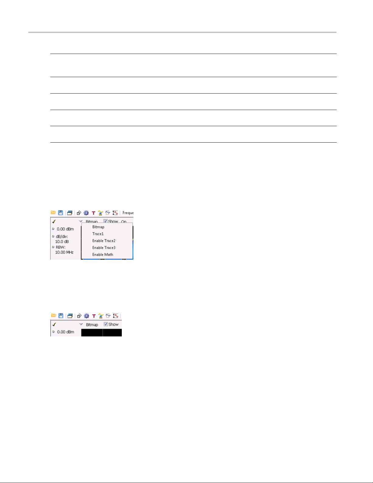
General Signal Viewing DPX Display

Trace Description

Bitmap

+Peak detecte

–Peak detected

Average detected

Math Trace

xxx

Displays the density of acquired data. The number of data points acquired at each pixel (representin by color.

Line trace. Displays the maximum values acquired in each update. Normal and Hold functions are available for this trace.

Line trace. Displays the minimum values acquired in each update. Normal and Hold functions are availab

Line trace. functions are available for this trace.

Line trace. Displays the difference between two traces. The two traces used are set in the Traces tab of the Settings panel.

g a particular amplitude level at a speciﬁc frequency at a point in time) is indicated

le for this trace.

Displays the average of all the values acquired in each update. Normal and Hold

Determining Which Trace Types Are Displayed

You can see the status of all the traces by selecting the Trace drop-down list. Traces that are not displayed are preceded by "Enable". In the following ﬁgure, you can tell that the Bitmap and -Peak Trace traces are displayed but the +Peak, Average, and Math Traces are not displayed.

Selecting Enable -Peak Trace from the Trace list displays the -Pea k detected values trace.

an see whether a trace is enabled by looking at its Show check box. The "se lected trace" is selected

You c in the Trace list. The Show check box is checked when the selected trace is enabled. To the right of the show box are readouts for detection of the selected t race (+Pk, Avg (VRMS), ) and its f unction (Hold, Normal,). You can enable/disable the selected trace by checking or unchecking Show.

Selecting Traces for Display – Standard Instrument

To select a trace for display:

68 RSA6000 Series & RSA5000 Series Printable Online Help

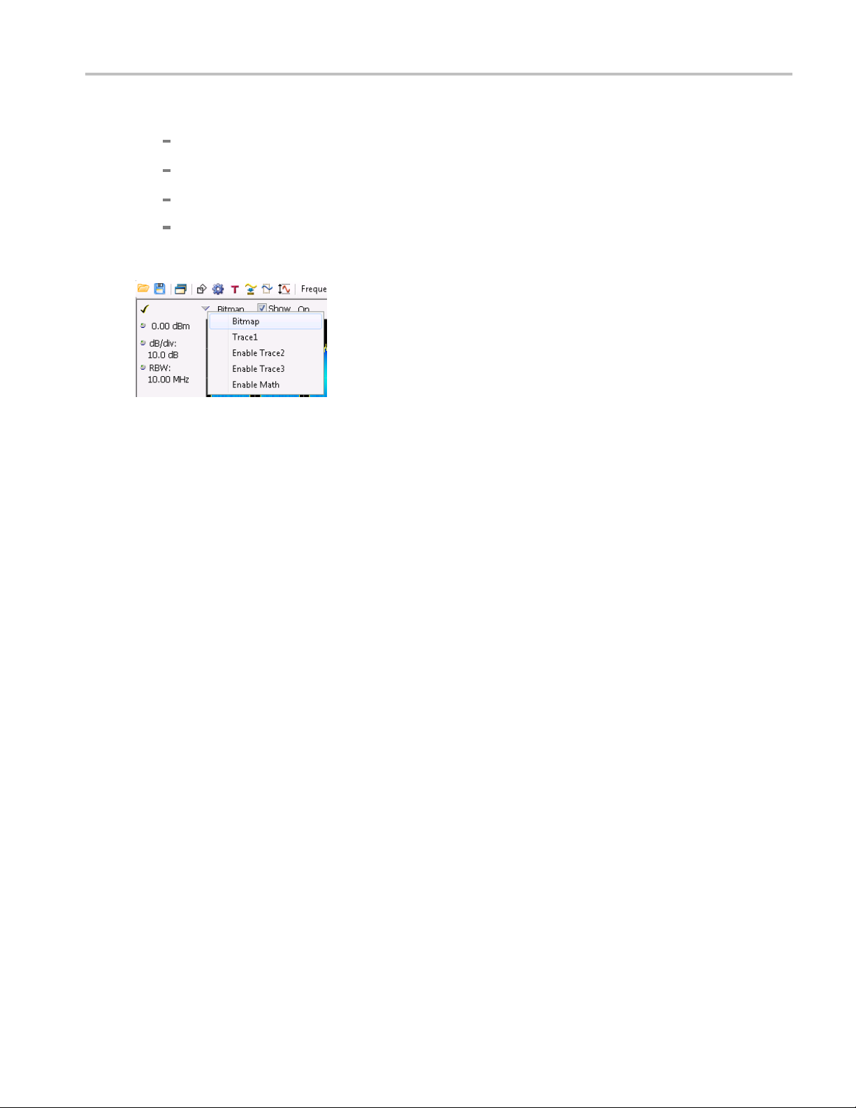
General Signal Viewing DPX Display

1. Use the Settings control panel:

Select Setup > Settings or click the Settings button.

Select the Trac es tab.

Select the trace from the drop-down menu.

Select the S

2. Select a trace from the Trace drop-down list.

Specify

You control how the +Peak, –Peak and Average (Avg (VRMS)) traces are displayed from the Traces tab of the Set from single updates or results collected over multiple updates.

To cha

1. Select Setup > Settings or click the Settings button.

2. Select the Trac es tab.

ing How +Peak, –Peak, a n d Average Traces Are Displayed

tings control panel. From the Traces tab, you can also specify whether these traces display results

nge how the traces are displayed:

how check box.

3. Select the trace type from the drop-down list.

4. If you select +Peak Trace or -Peak Trace, use the Function drop-down list to select either Normal or Hold.

a. Select Normal to set the trace to display the maximum/minimum values acquired in each

individual update.

b. Select Hold to set the trace to display the maximum/minimum values acquired over time. The

trace values are updated only if they exceed the existing values.

5. If you select Avg (VRMS) or Avg (of logs), use the Function drop-down list to select either Normal, Average (V RMS ),orAvg (of logs).

a. Select Normal to set the trace to display the average values acquired in each update.

b. Select Average (VRMS) or Avg (of logs) to set the trace to display an average of the average

values. Use the Count box to enter the number of times the trace is averaged.

RSA6000 Series & RSA5000 Series Printable Online Help 69

General Signal Viewing DPX Display

Available Traces for Display – Option 200 Instrument

Five traces can be shown in the DPX Spectrum, Zero Span, Frequency, and Phase displays– one bitmap and four line traces. The default traces are Bitmap and Trace 1. The other three traces are 2, 3, and Math. Line traces 1, 2, and 3 have user-selectable Detection and Function settings. The ﬁnal line trace is Math, allowing you

For the DPXogram display, only one trace is available — the DPXogram trace.

For the Split display, which consists of a DPXogram display on the top half and a DPX Spectrum display on the bottom half, you can display the Bitmap trace, Trace 1, Trace 2, Trace 3, Math trace, and Ogram Line (the s

to subtract one line trace from another.

elected line from the DPXogram display) on the bottom half of the display.

Selecting Traces for Display – Option 200

This is done almost the same as with the standard instrument, except that the choices available for Trace are different. Instead of +Pk, –Pk, and Avg traces, you select Trace 1, 2, and 3 and independently set the Detection method for each of these traces to +Pk, -Pk, Avg (VRMS), or Avg (of logs).

Reference. Changing the DPX Spectrum Display Settings

(see page 264)

70 RSA6000 Series & RSA5000 Series Printable Online Help

General Signal Viewing DPX Settings

DPX Settings

Menu Bar: Setup > Settings

Front Panel / Application Toolbar: Settings

The measurement settings for the DPX display are shown in the following table.

Settings tab

Freq & Span (see page 110) Sets frequency and span parameters for the DPX display. This tab appears for the

Params (see page 72) Sets sweep time and scroll settings. This tab appears only for the DPX Zero Span,

Freq & BW (

BW (see page 115) Sets Resolution Bandwidth.

Traces (Bitmap) Tab (see page 73)

Traces Tab (see page 76) Allows you to select the number and types of traces to display and their functions.

Traces (Math) Tab (see page 115)

Horiz page 79)

Bitmap Scale Tab (see page 80)

Amplitude Scale Tab (see

pag

me Freq Scale Tab

Ti page 82)

Prefs (see page 118) Speciﬁes whether certain display elements are visible.

Density (see page 83) Speciﬁes location and size for the DPX Density measurement box. ( Spectrum display

Audio Demod (see page 84) Enables and sets parameters for audio demodulation function.

xxx

see page

&VertScaleTab

81)

73)

(see

Description

Spectrum and DPXogram displays.

DPX Freque

TheFreq& Span, DPX Frequency, and DPX Phase views.

Allows you to conﬁgure the Bitmap Trace.

Allows you to conﬁgure the Math Trace.

Sets t

Sets the DPX Bitmap display parameters.

The Amplitude Scale tab allows you to change the vertical scale and offset, enable the 3-D

e Time and Freq Scale tab allows you to change the vertical and horizontal scale

Th settings, number of points in the trace, and Time resolution.

only; requires Option 200)

ncy and DPX Phase displays.

BW tab speciﬁes frequency and bandwidth parameters for the DPX Zero

he vertical and horizontal scale parameters for all the DPX views.

Waterfall display, and set the color scheme used for the DPXogram trace.

RSA6000 Series & RSA5000 Series Printable Online Help 71

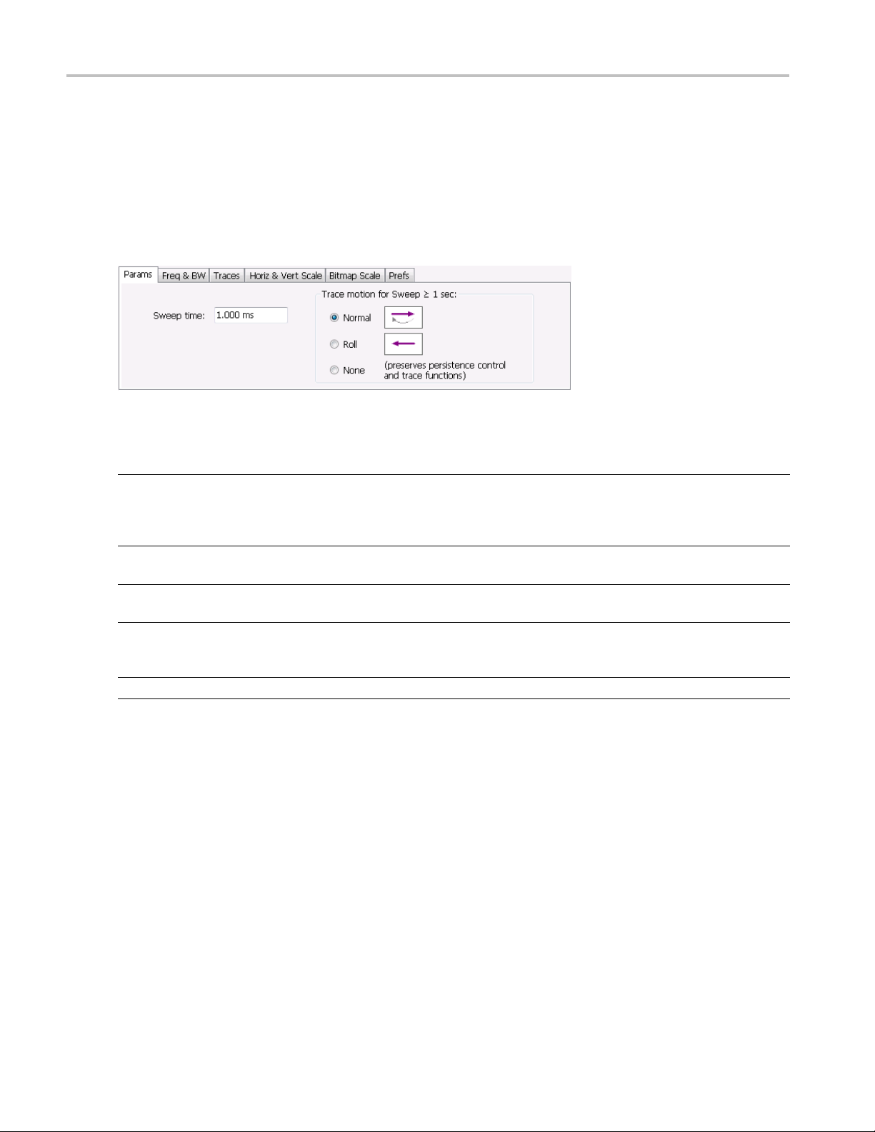
General Signal Viewing Params Tab – DPX Zero Span, DPX Frequency and DPX Phase Views

Params Tab – DPX Zero Span, DPX Frequency and DPX Phase Views

The Params tab sets the sweep time for the DPX Zero Span, Frequency and Phase views. Use the Params tab to set the scroll mode settings for the DPX Zero Span, Frequency and Phase views. In Scroll mode, points of the an acquisition is completed.

Params tab settings Zero Span, Frequency and Phase views

trace are plotted as they occur, as opposed to normal mode where the trace is plotted after

Setting

Sweep time Sets the time period for the measurement. By default, the Horizontal Scale is equal to

Trace motion for Sweep ≥ 1sec

Normal

Roll

None

xxx

Description

Sweep ti sweep time extends beyond the left and/or right edges of the graph. Range: 100 ns – 2000 s. Default: 1 ms.

Speciﬁes how the trace is displayed when the sweep time is equal to or greater than 1seco

Selec mode, a caret (^) moves below the graph to indicate the latest position.

Select Roll to scroll the trace as points are added at the r ight side of the graph. W hen Roll is selected, the trace moves to the left as points are added to the trace at the right side

Sel

me and the sweep covers 10 divisions. When the graph is zoomed in, the

nd.

t Normal to scroll the position at which data points are added to the trace. In this

of the graph.

ect None to display the trace without motion.

72 RSA6000 Series & RSA5000 Series Printable Online Help

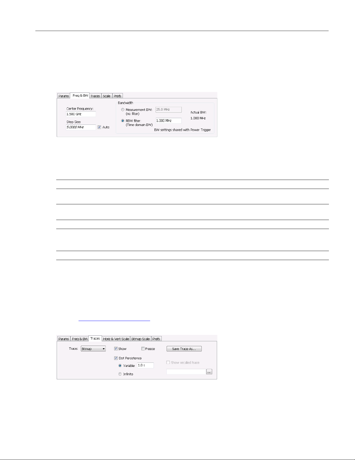
General Signal Viewing Freq & BW Tab – DPX Zero Span, DPX Frequency and DPX Phase Views

Freq & BW Tab – DPX Zero Span, DPX Frequency and DPX Phase Views

The Freq & BW tab speciﬁes frequency parameters for some of the DPX display views.

Freq & BW tab settings for the bitmap trace (Standard and option 200)

Setting

Center Frequency Sets the frequency at the center of the measurement bandwidth.

Step Size Sets the increment size when changing the Frequency using the knob or mouse wheel.

Auto

Measurement BW, no ﬁlter Speciﬁes the measurement bandwidth.

RBW (Time-domain BW) ﬁlter RBW (Time-domain BW) is a ﬁlter used to process the input signal before the system

Actual BW

xxx

Traces Tab – Bitmap

The Traces Tab allows you to set the display characteristics of displayed traces in the DPX display. The Traces tab for the DPX display has two versions: one for the DPX Bitmap trace (described in this topic) and one for line traces

Description

Arrow keys have an increment 10 times this setting.

When Auto is enabled, the step size is adjusted automatically based on Spectrum's span setting.

analyzes the signal. The ﬁlter value determines the acquisition bandwidth that the view requires. Range: 1 HZ to 60 MHz.

Shows the actual bandwidth being used for the display.

(see page 76).

Option 200 Traces tab (Bitmap trace)

RSA6000 Series & RSA5000 Series Printable Online Help 73

General Signal Viewing Traces Tab – Bitmap

Option 200 Tr

aces tab (DPXogram trace)

Traces tab settings for the bitmap trace (standard and option 200)

Setting

Trace

Show Speciﬁes

n (DPXogram trace

Detectio only)

Intensity (standard instrument only)

sistence

Dot Per

Variable The Variable dot persistence setting controls how long a point in the display is visible

Inﬁnite The Inﬁnite dot persistence setting prevents a point in the display from fading (not

Freeze Halts updates to the selected trace.

Save Trace As Saves the selected trace to a ﬁle for later recall and analysis.

Show Recalled Trace Displays a saved trace instead of a live trace (not available for the DPXogram trace).

xxx

Description

Select Bit

Sets the D methods are +Peak, -Peak, and Avg (VRMS).

Use Intensity to control the visibility of events. An increased intensity level allows a single, short event to be seen. This also makes such an event subject to the persistence contro events. Range is 1-100%. Resolution: 1.

Allows a dot to remain visible if it is not updated with new data. Choices for this setting are Variable and In ﬁnite. (Not available for the DPXogram trace.)

before fading (not available for the D PXogram trace). This setting has no units assoc

Standard instrument Range: 1–1000. Resolution 0.1.

Option 200 instrument Range: 50 ms–100 s.

ava

map or DPXogram to set the parameters of the DPX Bitmap or DPXogram trace.

whether or not the selected trace is displayed.

etection method

ls. This allows you to see the effect of the Persistence controls on infrequent

iated with it.

ilable for the D PXogram trace).

(see page 11 2) used for the trace. Available detection

Dot Persistence

Dot Persistence is the characteristic of the DPX display that determines how long a pixel in the display remains visible.

To set the Persistence:

1. Select Setup > Settings.

2. Select the Traces tab.

3. Select Dot Persistence.

74 RSA6000 Series & RSA5000 Series Printable Online Help

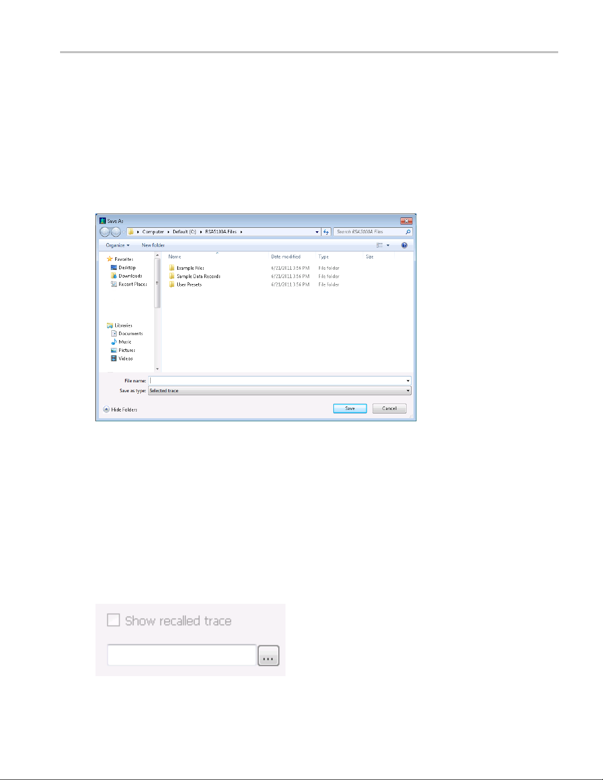
General Signal Viewing Traces Tab – Bitmap

4. Select either Inﬁnite or Varia b le.

5. If you select Variable, enter a value in the text box. The Variable persistence value can be set from 1 to

1000 in the base instrument, and from 0.05 to 100 seconds with Option 200.

Saving Trace

To save a trace for late r analysis:

1. Select the Save Trace As button. This displays the Save As dialog box.

2. Navigate to the location where you want to save the ﬁle.

3. Type a name for the saved trace and click Save.

Show Recalled Trace

You can recall a previously saved trace for comparison to a live trace. First, specify a trace for recall and second, enable Show Recalled Trace.

To select a trace for recall:

1. Select the ... button to display the Open dialog box.

RSA6000 Series & RSA5000 Series Printable Online Help 75

General Signal Viewing Traces Tab

2. In the Open dialog, navigate to the location of the saved trace.

3. Select the desired trace ﬁle.

4. Select OK to complete your selection.

5. Select the Show recalled trace check box.

6. Verify that the trace's Show check box is selected (either on this tab or next to the drop-down list

located at the top-left corner of the graph).

Traces Tab

The Traces Tab allows you to set the display characteristics of displayed traces in the DPX display. The Traces tab for the DPX display has two versions. One for non-Bitmap traces (described in this topic) and one for the DPX Bitmap trace

(see page 73).

Option 200 Traces tab

Setting

Trace drop-down list

Show Speciﬁes whether or not the trace shown in the Trace setting is displayed.

Freeze Halts updates to the selected trace.

Detection (Option 200 only) Sets the Detection method used for the trace. Available detection methods are +Peak,

Function

Save Trace As Saves the selected trace to a ﬁle for later recall and analysis.

Show Recalled Trace Displays a saved trace instead of a live trace.

Count Enables user adjustable number of averages. This setting is only present when Function

xxx

Description

Selects which trace to conﬁgure. For standard instruments, the available traces are Bitmap, +Peak detected, -Peak detected, Average, and Math. In instruments with Option 200, the available traces are Bitmap, Trace 1, Trace 2, Trace 3, and Math.

-Peak, and Avg (VRMS). Not all detection methods are available in all displays.

Selects the trace processing method. Available settings are: Normal, Average, and Hold.

= Average.

Detection

Trace Detection occurs when the trace is being decimated by the measurement. For example, if the maximum number of trace points is 100,000, and the selected analysis region is 200,000 samples, the

76 RSA6000 Series & RSA5000 Series Printable Online Help

General Signal Viewing Traces Tab

measurement must decimate the 200,000 resulting trace points by 2 to prevent exceeding the 100,000 trace point limit. Since only one value can be selected for each trace point, an algorithm must be used to select (detect) the a

ppropriate value to use.

The available detection methods are:

+Peak – Each point on the trace is the result of detecting the positive peak value present in the set of IQ samples available to that trace point.

-Peak – Each point on the trace is the result of detecting the negative peak value present in the set of IQ samples available to that trace point.

Avg (VR MS) [Average V

] – Each point on the trace is the result of determining the RMS Voltage

RMS

value for all of the IQ samples available to the trace point. When displayed in either linear (Volts, Watts) or

Log (dB, dBm), the correct RMS value results. When the averaging function is applied to a trace, the averaging is performed on the linear (Voltage) values, resulting in the correct average for RMS values.

NOTE. The Detection setting does not affect the trace until the spectrum length is longer than the Auto setting.

DPX Tr

ace Processing

The +Peak, -Peak, and Average traces can be processed to display in different ways. The Function setting

ols trace processing.

contr

Hold - Displays the value in the trace record for each display point. Each new trace display point is

ared to the previous maximum value and the greater value is retained for display and subsequent

comp comparisons. Available for traces using +Peak or -Peak detection.

mal - Displays the trace record for e ach display point without additional processing. Available

Nor

for all detection selections.

erage - Default setting for the Average. Multiple traces are averaged together to generate the

displayed trace. There is one vertical value for each underlying frequency data point. Once the speciﬁed number of traces have been acquired and averaged to generate the displayed trace, each new trace takes the place of the oldest trace in the calculation. The Count setting speciﬁes how many traces are averaged. Available for traces using Average detection.

Trace averaging uses the exponential method. If Count = 10, the newest trace's contribution to the averaged trace is 10%. When Count is not checked, the algorithm assumes the maximum number of traces contributing to the average is

Saving Traces

To save a trace for late r analysis:

1. Select the Save Trace As button. This displays the Save As dialog box.

RSA6000 Series & RSA5000 Series Printable Online Help 77

General Signal Viewing Traces Tab

2. Type a name for the saved trace and click Save.

Recalling Traces

You can recall a previously saved trace for comparison to a live trace. First, specify a trace for recall and second, enable Show Recalled Trace.

To select a trace for recall:

1. Click the ... button to display the Open dialog box.

2. Navigate to the desired ﬁle and click Open.

3. Check the Show Recalled Trace check box.

4. Verify that the trace's Show check box is selected (either on this tab or next to the drop-down list

located at the top-left corner of the graph).

78 RSA6000 Series & RSA5000 Series Printable Online Help

General Signal Viewing Horiz & Vert Scale Tab

Horiz & Vert Scale Tab

The Horiz & Vert Scale tab allows you to change the vertical scale settings used for the Bitmap trace. Changing the scale settings changes how the trace appears on the display but does not change control settings suc

h as Measurement Frequency.

Setting

Vertical

Description

Controls the vertical position and scale of the trace display.

Scale Changes the vertical scale.

Offset Adjusts the Reference Level away from the top of the trace display.

Reset Scale Sets Scale to its default value and Offset to zero. Disabled when Units (Setup > Analysis

> Units) is set to Watts or Volts.

Autoscale

Resets the scale of the vertical axis to contain the complete trace. Disabled when Units (Setup > Analysis > Units) is set to Watts or Volts.

Horizontal

Controls the horizontal position and scale of the trace d isplay.

Scale Changes the horizontal scale.

Position

Autoscale

Adjusts the horizontal position of the signal. This does not change the center frequency.

Resets the scale of the horizontal axis to contain the complete trace.

RSA6000 Series & RSA5000 Series Printable Online Help 79

General Signal Viewing Bitmap Scale Tab

Bitmap Scale Tab

The Bitmap Scale tab allows you to set the color scheme used for the Bitmap trace. Changing the DPX bitmap Color, Max and Min scale settings changes how the trace appears on the display but does not change contr

ol settings such as Measurement Frequency.

Setting

DPX Bitma

Curve Adjus

Auto

xxx

p (Signal Density)

Color Allows y

Max

Min

Color

Description

Controls

Sets the densities greater than this value.

Range: 1p% - 100%; D efault: 100%.

Sets the hit density represented by the bottom of the color range. Range: 0 - 80%; Defau

= 1), or it can be set to concentrate the resolution on the lower level of the range (Curve >

1) or the mapping can be set to show the best resolution on the upper range of density or hi

Adju

the appearance and scale of the DPX Bitmap trace.

ou to select the color palette used for the DPX Bitmap trace.

hit density represented b y the top of the color scale. "Clipping" occurs for

lt: 0.

ts how colors are mapped to the signal density. The mapping can be linear (Curve

t count (Curve < 1).

sts the Max and Min settings to display the broadest range of colors.

80 RSA6000 Series & RSA5000 Series Printable Online Help

General Signal Viewing Amplitude Scale Tab

Amplitude Scale Tab

The Amplitude Scale tab allows you to change the ver tical and horizontal scale settings, enable the 3-D Waterfall display, and set the color scheme used for the DP Xogram trace.

Setting

Height

Description

Height controls apply only to the 3-D Waterfall display.

Scale Changes the vertical scale for trace Amplitude in the graph (not the vertical scale for

Time).

Position

Speciﬁes the level displayed at the bottom edge of the graph. (Bottom front edge in the 3-D view).

Autoscale

Adjusts the vertical position bottom for linear units like Amps and Volts. Adjust the vertical position top for log units like dBm. dBm is the default.

3-D Waterfall Displays the DPXogram in a 3-D format.

Northeast

Shifts the perspective of the 3-D graph so that the oldest traces move back and to the right.

Northwest

Shifts the perspective of the 3-D graph so that the oldest traces move back and to the left.

Reset Scale Resets the Height and Color settings to their default values.

Color (DPXogram)

Color D isplays a drop-down list that allows you to set the color scheme used for the DPXogram

trace.

Max

Min

xx x

Sets the power level represented by the top of the color scale.

Sets the power level represented by the bottom of the color scale.

RSA6000 Series & RSA5000 Series Printable Online Help 81

General Signal Viewing Time & Freq Scale Tab

Time & Freq Scale Tab

The Time and Freq Scale tab allows you to change the vertical and horizontal scale settings, set the time resolution and number of trace points of the DPXogram display.

Setting

Vertical (time)

Time/div For most Spectrogram applications. Primary time scale control is Time/div. Time

Position

Time at position

Reset Scale Sets the Time/div and Position settings to their default values.

Trace Points

Time resolution

Auto

Capacity Readout of the total length of time that can be captured. This readout is provided

Horizontal (frequency)

Scale Sets the displayed frequency range of the graph. This control affects only visual

Position

Autoscale

xxx

Description

scale can be zoomed in or out when acquisitions are s topped.

The position of the DPXOgram record at the bottom of the display. Position cannot be changed while acquisitions are active, and is reset to zero when acquisitions are started again.

Displays the time of the DPXogram line shown at the bottom o f the graph. This time is relative to the Time Zero Reference of the current acquisition. If Position is set to a negative value, the Time at position readout will be blanked.

Sets the number of trace points computed for each DPXogram line. These are the points used for marker measurements and for results export.

Speciﬁes the length of time represented by each line in the graph.

Sets the time represented by each line in the graph to be adjusted by the analyzer checked) or manually (when unchecked). When Auto is enabled, Time Resolution change based on Time/div.

so that you can see how changing the Trace Points and Time resolution affects the amount of data that can be captured. Capacity is represented in the format dd:hh:mm:ss.

scaling, and does not change the acquisition or analysis parameters.

Sets the frequency displayed at the center of the graph. Changing this value does not change the Frequency setting.

Sets the frequency scale to the Spectrogram Span value.

82 RSA6000 Series & RSA5000 Series Printable Online Help

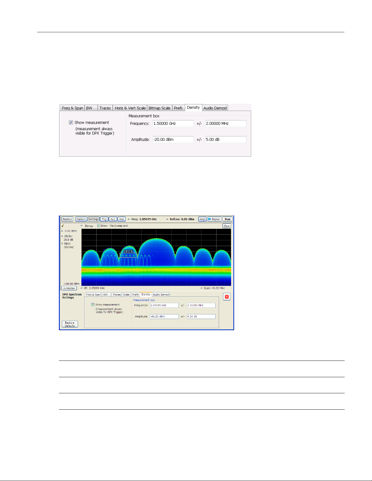
General Signal Viewing Density Tab – Option 200

Density Tab – Option 200

The Density tab speciﬁes the parameters of the measurement box used for measuring average signal density of an area in the bitmap. The measurement box is also used by DPX Density triggering.

To measure the average signal density over a rectangular portion of the DPX bitmap, you c

an adjust the size and location of the measurement area using these controls, or by dragging the measurement box in the graph. You move the box by dragging the readout. You adjust the size of the box by dragging the corners or edges.

Setting

Show Measurement Shows or hides the measurement box in the graph when Triggering is not set to DPX

Frequency

Amplitude

xxx

Description

Density. If Triggering is set to DPX Density, the measurement box is always visible.

Speciﬁes the frequency at the center of the measurement box. The +/- value speciﬁes the width of the measurement box.

Speciﬁes the amplitude of the center of the measurement box. The +/- value speciﬁes the height of the measurement box.

RSA6000 Series & RSA5000 Series Printable Online Help 83

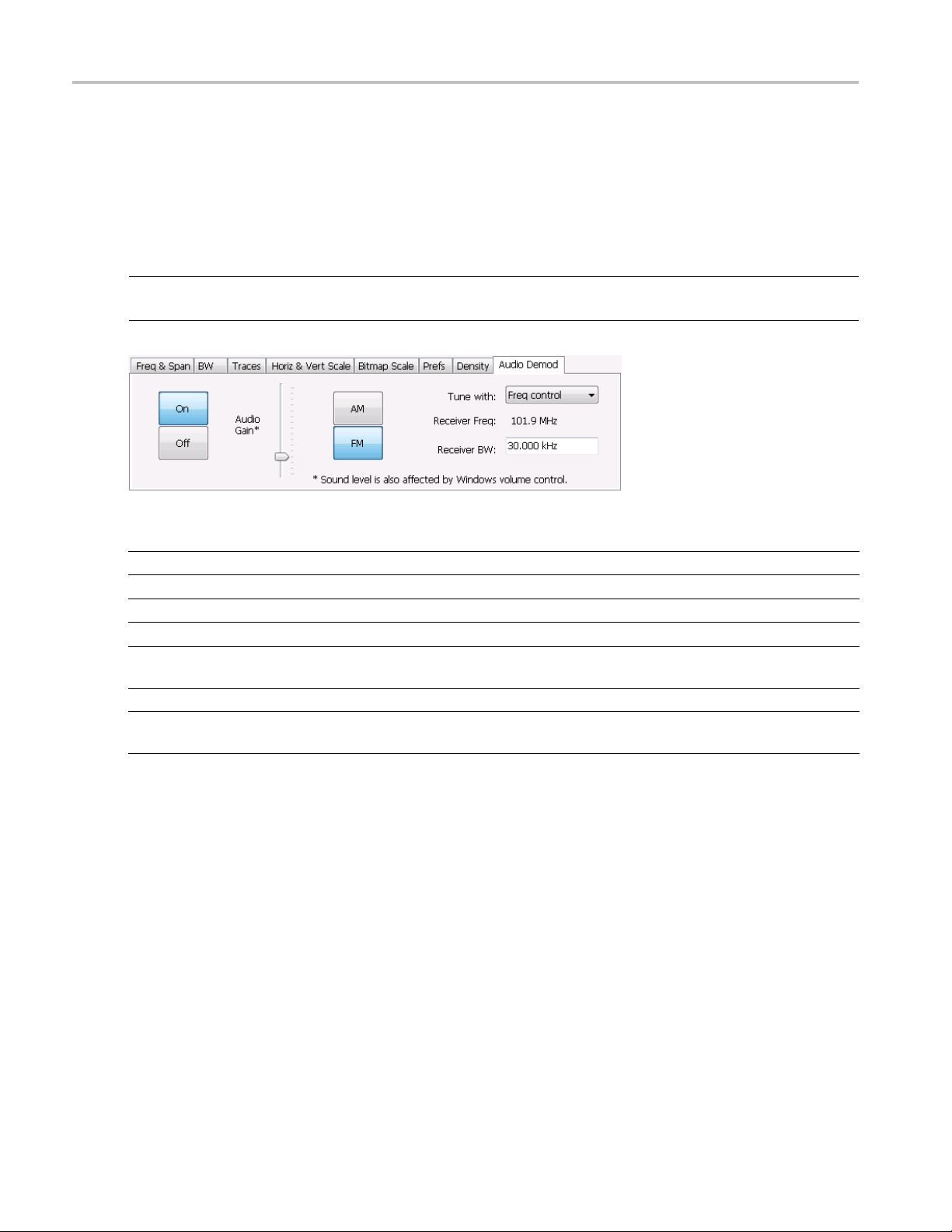
General Signal Viewing Audio Demod Tab

Audio Demod Tab

Audio demodulation can help you identify unknown radio signals. You control the audio demodulation function with the Audio Demod tab. You access the Audio Demod tab from the Settings control panel of the DPX displ

NOTE. Audio Demodulation is available only in real-time acquisition mode (not swept acquisition), and the Trigger mode must be set to Free Run (not Triggered).

ay.

Setting

On/Off Enables/disables audio demodulation.

Audio Gain Adjusts the volume of the demodulated audio.

Tune with

Receiver Freq

Receiver BW

xxx

Description

Selects Amplitude Modulation as the demodulation method.

Selects Frequency Modulation as the demodulation method.

Speciﬁes how the frequency to be demodulated is speciﬁed. You can select markers or the frequency control.

Readout of the frequency to be demodulated.

Adjusts the equivalent receiver bandwidth for the audio demodulation. The range of values is 1 kHz to 500 kHz.

AM / FM

Note that these buttons select the demodulation method; they do not specify a frequency band.

Tune with

The choices for this setting are: one of the markers (MR, M1, M2, M3, M4) or the Frequency control (either the front-panel knob or the Freq control in the application).

To use a marker to specify the frequency to be demodulated:

1. Select Markers > Deﬁne Markers to display the Deﬁne Markers control panel.

2. Select Add to turn on the next marker.

84 RSA6000 Series & RSA5000 Series Printable Online Help

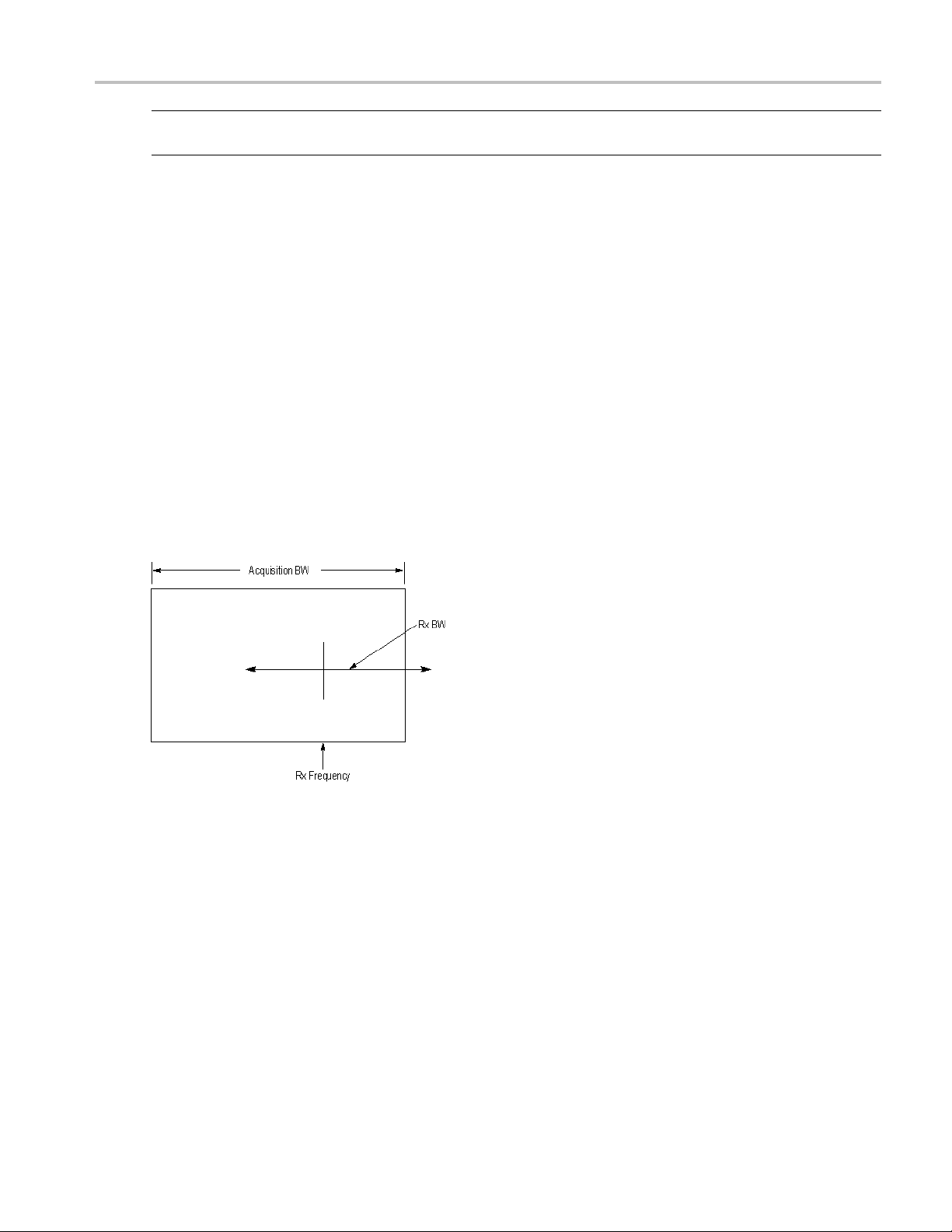
General Signal Viewing Audio Demod Tab

NOTE. The ﬁrst marker deﬁned will always be MR. The MR marker is the reference for delta marker readouts.

3. Select the trace to which the marker should be attached from the drop-down list.

4. Click Add to a

5. Click the close button to remove the Deﬁne Markers control panel.

Select markers. Select one of the markers in the Tune with drop-down list and then set the location of the

marker to the frequency you want to demodulate. If the marker you select is not enabled, the analyzer will tune to the frequency the marker was last set to.

dd additional markers. Assign them to the appropriate trace.

Receiver BW

The Receiver BW setting will not change the acquisition bandwidth. Thus, if the acquisition bandwidth is too narrow, audio demodulation will be disabled. The following three cases illustrate the relationship between

Case 1. In this case, the upper limit of the Receiver BW exceeds the upper limit of the acquisition

bandwidth. When this occurs, audio demodulation is disabled and an error message is displayed.

the A cquisition BW, Receiver Frequency, and Receiver BW.

Case 2. In this case, the upper and lower limits of the Receiver BW exceed the upper and lower limits

the acquisition bandwidth. When this occurs, audio demodulation will be disabled and an error

of message is displayed.

RSA6000 Series & RSA5000 Series Printable Online Help 85

General Signal Viewing Time Overview Display

Case 3. In t

limits of the acquisition bandwidth. This is the desired relationship between the three settings, and audio demodulation is enabled.

his case, the upper and lower limits of the Receiver BW fall within the upper and lower

Time Overview Display

The Time Overview display shows the entire acquisition record and shows you how the spectrum time and analysis time ﬁt within the acquisition record. This enables you to see how you can adjust the spectrum time and analysis time to m easure portions of the data.

You can specify the maximum number of trace points in the Time Overview display. You can set the maximum number of trace points to 1K, 10K, 100K, 1M points or to Never decimate. If the Acquisition Length includes more than 10,000 sample points (and Max trace points is not set to Never decimate), the trace is decimated (using the +Peak method, similar to +Peak detection in a Spectrum display) to 10,000 points. This dec imated trace is what is used for marker measurements.

The Time Overview window displays the Spectrum Length and Analysis Length. The Spectrum Length is the period of time within the acquisition record over which the spectrum is calculated. The Analysis Length is the period of time within the acquisition record over which all other measurements (such as Amplitude vs. Time) are made. The Spectrum Length and Analysis Length can be locked together so that the data used to produce the Spectrum display is also used for measurement displays; however, they

86 RSA6000 Series & RSA5000 Series Printable Online Help

Tektronix RSA6106A, RSA6114A, RSA6120A, RSA5103A Online Help

Specifications and Main Features

Frequently Asked Questions

User Manual