

Page 1

xx
PSM3000, PSM4000,
and PSM5000 Series
ZZZ
RF and Microwave Po wer Sensors/Meters
User Manual
*P077059201*
077-0592-01
Page 2

Page 3

xx
PSM3000, PSM4000,
and PSM5000 Series
ZZZ
RF and Microwave Power Sensors/Meters
User Manual
www.tektronix.com
077-0592-01
Page 4

Copyright © Tektronix. All rights reserved. Licensed software products are owned by Tektronix or its subsidiaries
or suppliers, and are protected by national copyright laws and international treaty provisions.
Tektronix products are covered by U.S. and foreign patents, issued and pending. Information in this publication
supersedes that in all previously published material. Specifications and price change privileges reserved.
TEKTRONIX and TEK are registered trademarks of Tektronix, Inc.
Contacting Tektronix
Tektronix, Inc.
14150 SW Karl Braun Drive
P.O. B o x 5 0 0
Beaverto
USA
For product information, sales, service, and technical support:
n, OR 97077
In North America, call 1-800-833-9200.
Worl dwid e, vis it www.tektronix.com to find contacts in your area.
Page 5

Warranty
Tektronix warrants that this product will be free from defects in materials and workmanship for a period of three
(3) years from the date of shipment. If any such product proves defective during this warranty period, Tektronix, at
its option, either will repair the defective product without charge for parts and labor, or will provide a replacement
in exchange for the defective product. Parts, modules and replacement products used by Tektronix for warranty
work may be n
the property of Tektronix.
ew or reconditioned to like new performance. All replaced parts, modules and products become
In order to o
the warranty period and make suitable arrangements for the performance of service. Customer shall be responsible
for packaging and shipping the defective product to the service center designated by Tektronix, with shipping
charges prepaid. Tektronix shall pay for the return of the product to Customer if the shipment is to a location within
the country in which the Tektronix service center is located. Customer shall be responsible for paying all shipping
charges, duties, taxes, and any other charges for products returned to any other locations.
This warranty shall not apply to any defect, failure or damage caused b y improper use or improper or inadequate
maintenance and care. Tektronix shall not be obligated to furnish service under this warranty a) to repair damage
result
b) to repair damage resulting from improper use or connection to incompatible equipment; c) to repair any damage
or malfunction caused by the use of non-Tektronix supplies; or d) to service a product that has b een modified or
integrated with other products when the effect of such modification or integration i ncreases the time or difficulty
of servicing the product.
THIS WARRANTY IS GIVEN BY TEKTRONIX WITH RESPECT TO THE PRODUCT IN LIEU OF ANY
OTHER WARRANTIES, EXPRESS OR IMPLIED. TEKTRONIX AND ITS VENDORS DISCLAIM ANY
IMPLIED WARRANTIES OF MERCHANTABILITY OR FITNESS FOR A PARTICULAR PURPOSE.
TRONIX' RESPONSIBILITY TO REPAIR OR REPLACE DEFECTIVE PRODUCTS IS THE SOLE
TEK
AND EXCLUSIVE REMEDY PROVIDED TO THE CUSTOMER FO R BREACH OF THIS WARRANTY.
TEKTRONIX AND ITS VENDORS WILL NOT BE LIABLE FOR ANY INDIRECT, SPECIAL, INCIDENTAL,
OR CONSEQUENTIAL DAMAGES IRRESPECTIVE OF WHETHER TEKTRONIX OR THE VENDOR HAS
ADVANCE NOTICE OF THE POSSIBILITY OF SUCH DAMAGES.
[W4 – 15AUG04]
btain service under this warranty, Customer must notify Tektronix of the defect before the expiration of
ing from attempts by personnel other than Tektronix representatives to install, repair or service the product;
Page 6

Page 7

Table of Contents
Preface ............................................................................................................... v
Safety Information............................................................................................. v
About This Manual ............................. .................................. ............................. v
Products.......... ................................ ................................ .............................. vi
Key Features .................................................................................................. vi
Where To Find More Information ......................................................................... vii
Getting Started ..... . ... . . ..... . ..... . ... . . . .... . ..... . ..... . ... . . ..... . ..... . ... . . . .... . ..... . ..... . ... . . ..... . ..... 1
Install the Software ............................................................................................ 1
Connect to a Computer........................................................................................ 6
Start An
Functional Check ............................................................................................. 10
Operating Basics................................................................................................... 13
Measurement Capabilities . . ..... . .... . ..... . ..... . ..... . .... . . .... . ..... . ..... . ..... . .... . ..... . ..... . ..... . 14
CW (Average) Measurements ............... .................................. .............................. 14
Pulse Measurements.......................................................................................... 15
Puls
Configure Instrument for Measurements ................................................................... 17
Power Meter Application... .................................. ................................ .................... 19
Front Panel Elements......................................................................................... 19
Make an Average Power (CW) Measurement ................... ................................ .......... 27
Make a Pulse Measurement Using Duty Cycle........................ ................................ .... 28
Ma
Pulse Profiling Application................. .................................. ................................ .... 31
Menu Features................................................................................................. 31
Toolbar Functions............................................................................................. 36
Make a Marker Measurement ..................... ................................ .......................... 48
Make a Gated Measurement ....................... ................................ .......................... 49
High Speed Logger Application ..... ................................ .................................. .......... 52
Menu Functions............................................................................................... 53
Make a Simple Measurement................................................................................ 58
Troubleshooting........... ................................ ................................ .................... 59
Index
Application.......................................................................................... 10
eProfiling..................... ................................ .................................. .......... 16
ke a Pulse Power Measurement ................... ................................ ...................... 29
RF and Microwave Power Sensors/Met ers i
Page 8

Table of Contents
List of Figure
Figure 1: Power Meter application interface using a PSM5120........................................ ...... 19
Figure 2: Di
Figure 3: Pulse Profiling application interface ................................................................. 31
Figure 4: Gate positioning diagram ... .................................. ................................ ........ 44
Figure 5: Position of gates for measurement . . ..... . ... . . ..... . ..... . .... . . .... . ..... . ..... . .... . ..... . ..... . .. 51
Figure 6: High Speed Logger application window ...................... .................................. .... 52
agram of a burst time slot .......................................................................... 23
s
ii RF and Microwave Power Sensors/Meters
Page 9

List of Tables
Table i: Product documentation................................................................................. vii
Table 1 : F un
Table 2: Power Meter default values ................................ ................................ ............ 25
Table 3: Sweep time values ...................................................................................... 37
ctions by instrument model........................................................................ 13
Table of Contents
RF and Microwave Power Sensors/Meters iii
Page 10

Table of Contents
iv RF and Microwave Power Sensors/Meters
Page 11

Preface
Safety Information
Preface
About This Manual
Product gen
environmental compliance information for the products discussed in this manual
are located in the Installation and Safety Instructions. You can find this document
in print form in the box that shipped with your product, in electronic form on
the USB memory device in the box that shipped with your product, or online at
www.tektronix.com/manuals. Please refer to that document b efore installing
and using
This doc
Series, PSM4000 Series, and PSM5000 Series RF and Microwave Power
Sensors/Meters:
The Getting Started chapter provides an overview of instrument features,
installation instructions, and a functional check procedure. (See page 1.)
The Operating Basics chapter provides information about how measurements
work, how to configure the instrument for making measurements, and
information about averaging, pulse measurements, CW measurements, and
pulse profiling. (See page 13.)
The Power Meter Application chapter provides information about using this
application. (See page 19.)
eral safety information, EMC and safety compliance, and
this product.
ument contains the following information about the Tektronix PSM3000
The Pulse Profiling Application chapter provides information about using this
application. (See page 31.)
The High Speed Logger Application chapter provides information about using
this application. (See page 52.)
RF and Microwave Power Sensors/Met ers v
Page 12

Preface
Products
The Tektronix PSM3000 Series, PSM4000 Series, and PSM5000 Series RF
and Microwave Power Sensors/Meters convert radio frequency (RF) and
microwave power into digital data at the point of measurement. They are ideal
for troubleshooting and characterization in the lab, and can be used for radio
frequency (
RF) component testing. These products connect d irectly to a desktop
or laptop computer with a USB 2.0 port and cable.
Product Description Connector type
PSM3110 10MHz-8GHz
PSM3120 10MHz-8GHz
PSM3310 10MHz-18GHz
PSM3320 10MHz-18GHz
PSM3510 10MHz-26.5GHz
PSM4110 10MHz-8GHz
PSM4120 10MHz-8GHz
PSM4320 50MHz-18GHz
PSM4410 50MHz-20GHz
PSM5110 100MHz-8GHz
PSM5120 100MHz-8GHz
PSM5320 50MHz-18GHz
PSM5410 50MHz-20GHz
3.5mm-male
N-Type male
3.5mm-male
N-Type male
3.5mm-male
3.5mm-male
N-Type male
N-Type male
3.5mm-male
3.5mm-male
N-Type male
N-Type male
3.5mm-male
Key Features
Reading rates up to 2000 readings per second
Meters are calibrated over full temperature range: No zero or cal needed
before making measurements, saving time and avoiding poor-quality data
Average power, duty cycle corrected pulse power, and measurement logging
on all models
Max hold and relative measurement modes
Offset, frequency response, and 75 Ω minimum loss pad correction
Flexible averaging modes for quick, stable measurements
TTL trigger input and output allow synchronization with external instruments
Pass/Fail limit mode
The PSM3000 series offers True Average power measurements that give
accurate results re gardless of signal shape or modulation
vi RF and Microwave Power Sen sors/Meters
Page 13

Preface
The PSM4000 and
PSM5000 series offer average power, pulse power, duty
cycle, peak power, and crest factor measurements
The PSM5000 se
ries includes a Pulse Profiling application for making
measurements on repetitive, pulsed signals
Where To Find More Information
You c a n find more information about your instrument in the following
documents. These documents can be found on the Tektronix Web site at
www.tektronix.com/manuals, on the product documentation USB device that
shipped with your instrument, or both.
Table i: Product documentation
To read about Use these documents
Product compliance, safety, and
set up and installation information
Operation, configuration, and
application information
Specifications and field verification
procedures
Declassification and security Declassification and Security Instructions available for download at www.tektronix.com/manuals.
Programming information Programmer’s M anual available on the product documentation USB device that shipped with
Online help Online help is available in the SW application you load onto your computer when you first
Installation and Safety Instructions available printed, on the product documentation USB device
that shipped with your instrument, and for download at www.tektronix.com/manuals.
User manual (this manual) available in English, German, French, Spanish, Italian, P ortuguese,
Russian, Korean, Japanese, Simplified Chinese, and Traditional Chinese on the product
documentation USB device that shipped with your instrument and for download at
www.tektronix.com/manuals.
Specifications and Field Verification Technical Reference available on the product
documentation USB device that shipped with your instrument, and for download at
www.tektronix.com/manuals.
your instrument, and for download at www.tektronix.com/manuals.
install the instrument.
RF and Microwave Power Sensors/Meters vii
Page 14

Preface
viii RF and Microwave Power Sensors/Meters
Page 15

Getting Started
Install the Software
This section provides the following information:
How to install the software
How to install the U SB driver and connect to a computer
How to start and application and perform a functional check
Before connecting the instrument to a computer, you need to first load
the software provided on the USB memory device that shipped with your
instrument. You can also find the latest software on the Tektronix Web site at
www.tektronix.com/software.
Computer, System, and
USB Requirements
Compute
the instrument software must have at least 2 GB RAM and a USB 2.0 port that
supplies more than 450 mA at 5 V.
Power requirements. This instrument is powered through the USB cable when
connected to a computer. The USB 2.0 port of the computer must supply more
than
this product. The supplied cable has 20 AWG power conductors that are a heavier
gauge than most USB cables.
NOTE. Refer to the Specifications section of the PSM3000, PSM4000, and
PSM5000 Series RF and Microwave Power Sensors/Meters Specifications and
Field Verification Technical Reference for additional information on electrical
quirements.
re
Hub recommendations. A USB host port on a computer will provide adequate
power for the instrument under normal circumstances. However, if you use a
SB cable longer than 3 to 5 meters, are connecting multiple instruments, or
U
are using a portable computer that runs on battery power, you will need to use
an active or self-powered hub.
The instrument typically draws 450 mA at a nominal 5 VDC. An active hub
compensates for the DC voltage drop in a USB cable longer than 3 to 5 meters.
It also conserves battery life in a portable computer.
r hardware requirements. The computer onto which you are downloading
450 mA at 5 V. Tektronix recommends using the USB cable supplied with
System Requirements. The instrument software you are downloading is
compatible with the following operating systems:
RF and Microwave Power Sensors/Met ers 1
Page 16

Getting Started
Software Installation
Procedure
Windows XP, Ser
Windows Vista
Windows 7 (32 or 64-bit, or XP mode)
This procedure allows you to install one or more of the following software
applications or programs:
Power Meter application: provides a virtual power meter front panel for your
instrument. Use the application software to make power meter measurements.
High-speed Logging application: allows you to take raw, high-speed
readings from your instrument.
Pulse Profiling application: (PSM5000 series only) provides the tools for
complete characterization of a modulated signal.
Sample Code: provides programming examples for remote control of
the instrument. You can read more about remote programming in the
PSM3000, PSM4000, and PSM5000 Series RF and Microwave Power
Sensors/Meters Programming Manual available on the Tektronix Web site at
www.tektronix.com/manuals.
vice Pack 3
2 RF and Microwave Power Sensors/Meters
Page 17
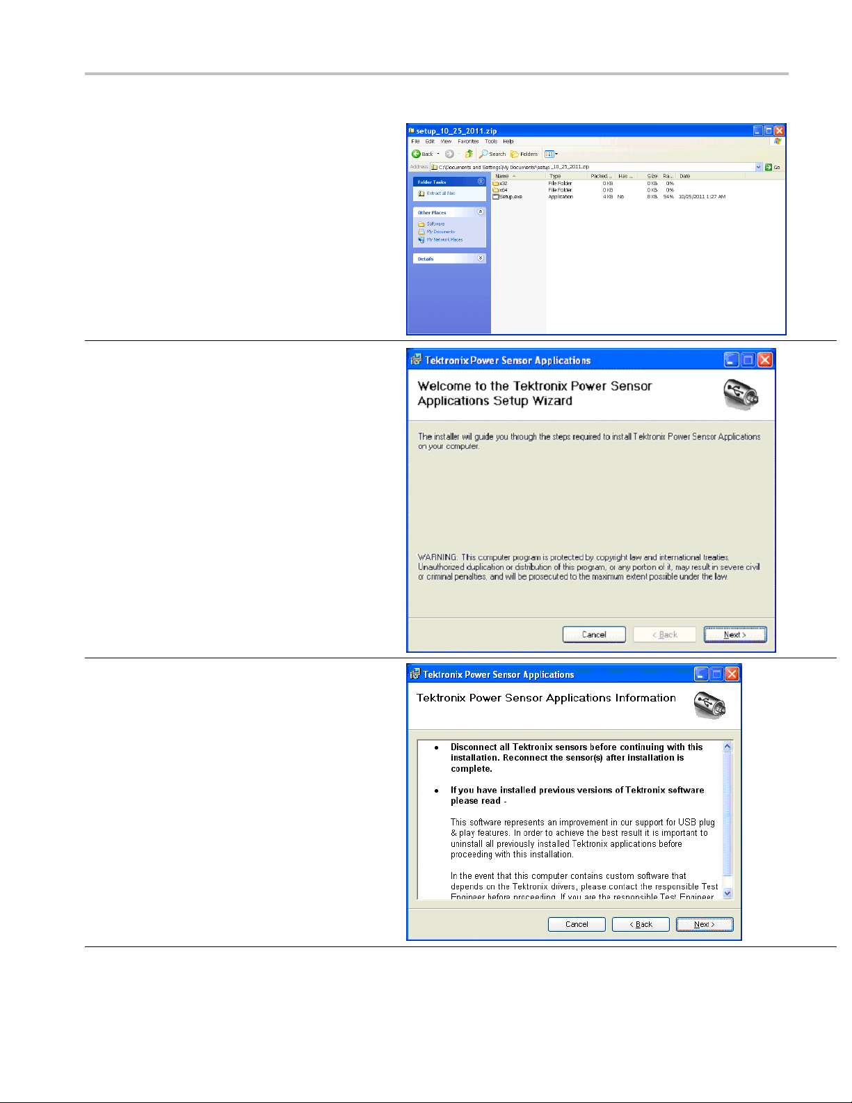
1
Go to www.tektronix.com and search for the most
recent software version for this product and download
it to your comp
the .exe file to start installation.
uter. Once downloaded, double click on
NOTE. You can also insert the USB memory device
that shipped
USB drive. The installation should start automatically.
If the installation does not start automatically, select
Start > Run and the media drive and a semicolon (D:
for example
setup.exe file you downloaded from the Tektronix Web
site, and then press OK.
2 The installer will open and guide you through the
installation procedure. Select Next to continue.
with your instrument into the computer
), and then \setup.exe or the location of the
Getting Started
3
If you have a previous version of the instrument
software, uninstall it before proceeding.
If you are ready to continue installation, click Next.
RF and Microwave Power Sensors/Met ers 3
Page 18
Getting Started
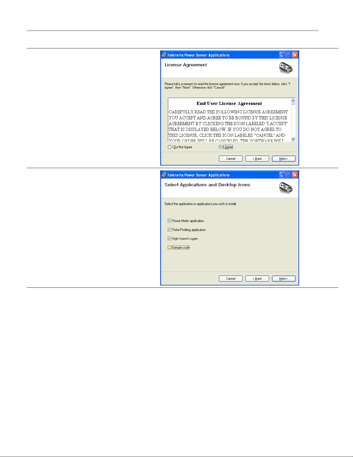
4 Read the licen
then click Next to continue.
5
The installer is ready to install the following software
on your computer (this will vary depending on options
and instrument model):
Power Meter application
Pulse Profiling application
High Speed Logger
Sample Code
Click Next to continue.
se agreement and select Iagreeand
4 RF and Microwave Power Sensors/Meters
Page 19

6
Confirm location for download or provide a location,
and then click Next.
7
When prompted, confirm installation by selecting Next.
Getting Started
RF and Microwave Power Sensors/Met ers 5
Page 20
Getting Started
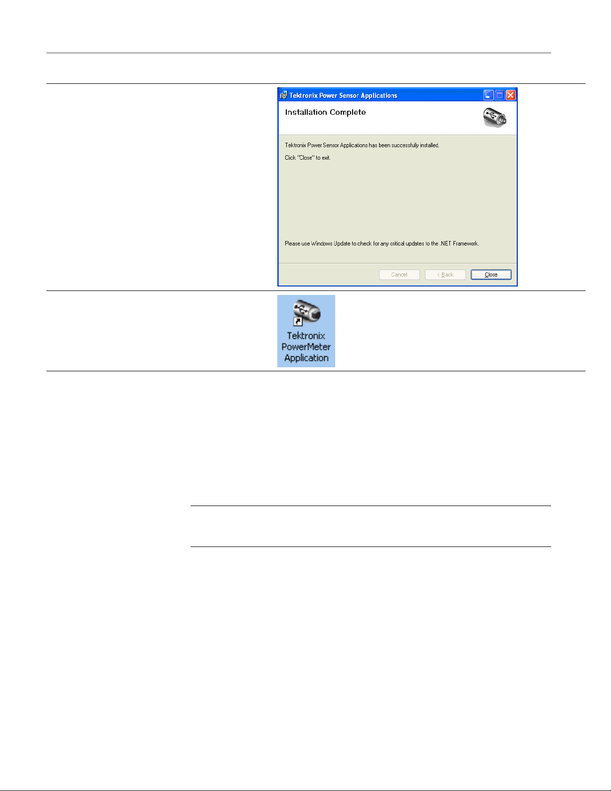
8 When the insta
appear stating that the software was successfully
installed. Select Close to exit.
9 Each downloaded application will now have an
associated icon on the Desktop of your computer.
Before opening the application, connect the instrument
to your computer. (See page 6, Connect to a
Computer.)
llation is complete, a dialog box will
Connect to a Computer
Install the USB Driver
This in
strument is powered through a USB cable that you attach to a computer.
Use the following procedure to install the USB driver so that the computer can
communicate with the instrument. Once the driver is installed, you can start the
Power Meter application software and any other instrument applications that
were installed.
NOTE. Tektronix recommends using the USB cable supplied with this product.
upplied cable has 20 AWG power conductors that are a heavier gauge than
The s
most USB cables.
6 RF and Microwave Power Sensors/Meters
Page 21
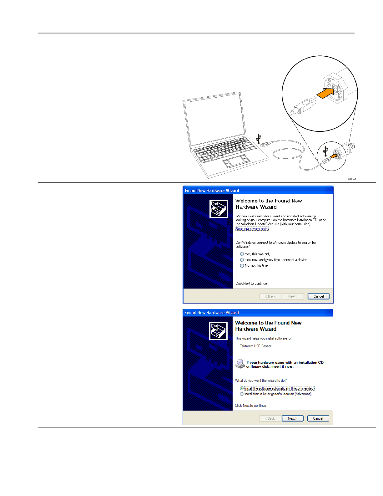
1
Use a USB-A to USB-B interface cable to connect the
instrument to the computer.
2 A Welcome to the Found New Hardware Wizard dialog
box will appear. Select Yes, this time only and then
select Next to continue.
Getting Started
3
Select Install the software automatically
(Recommended) and then select Next to continue.
RF and Microwave Power Sensors/Met ers 7
Page 22

Getting Started
4
The W izard will search for the appropriate software.
Once found, the driver will install.
5
The Wizard will show you when the installation is
complete. Select Fin ish.
You can now open the Power Meter application or
other instrument applications that were installed.
8 RF and Microwave Power Sensors/Meters
Page 23

Getting Started
Connect Multiple
Instruments
LED Indicator
If you are conne
The USB port or hub must supply more than 450 mA at 5 VDC for power
instrument operation. Read more about USB power requirements. (See page 1,
Computer, System, and USB Requirements.)
There is a green LED located below the trigger out (TO) connector on the
ment. This LED indicates instrument status as follows:
instru
cting more than one instrument to a computer, use a USB hub.
Dim green and steady: This shows power is being supplied to the instrument
at the instrument has not yet been recognized by the computer.
but th
Bright green and steady: This is the state for normal operation and shows that
r is being supplied to the instrument and that the instrument has been
powe
recognized.
ght green and blinking: This state shows that the instrument is not getting
Bri
enough current from the USB port. This usually means that the USB port
is not a high current USB 2.0 port.
Bright green and blinks a few times: This state is activated when you have
requested the software to identify the instrument. This is useful when you have
multiple instruments connected at once. (See page 10, Start An Application.)
RF and Microwave Power Sensors/Met ers 9
Page 24

Getting Started
Start An Appli
cation
Functional Check
To start an application, double-click the appropriate icon on the Desktop of your
computer, or select it from its program location on your computer (for example,
through the S
NOTE. An application will not launch unless the instrument is connected to the
computer.
If you are u
application software for each instrument. Each instance of the software identifies
its corresponding instrument by displaying the model, serial number, and port
address in the software window title bar.
To identify which instrument corresponds to which software window, compare
the serial number displayed in the software to the serial number stamped on the
instrument body below the USB port. Or, click Sensor ID in the application,
which causes the instrument LED to blink four times.
tart menu).
sing multiple instruments, you must open a new instance of the
After you have installed the software and connected the instrument to a computer,
orm this functional check to verify that your instrument is operating correctly.
perf
You will need the following equipment to perform the functional check:
Equipment Part number
RF/Microwave Source
Windows PC, with Power Meter application
installed
USB cable
Adapters, as needed, to connect RF source
to instrument
Agilent N5183A or equivalent
—
174-6150-00
—
10 RF and Microwave Power Sensors/Meters
Page 25

Getting Started
Warm Up Procedure
Functional Check
Procedure
1. For 24 hours pri
instrument must be stored in a stable laboratory environment. In addition, the
instrument should be powered for at least 20 minutes before starting the test.
Stable environmental conditions are defined as:
Temperature: 20 °C to 30 °C (68 °F to 86 °F)
Humidity: 15% to 95% noncondensing
Altitude: S
2. All equipment requiring power should be connected to mains and warmed up
according
1. Connect the instrument to the computer with a USB cable if you have not
already done so.
2. Turn on and preset a signal source.
3. Turn the source RF output off.
4. Connect the source to the instrument input connector. (Use adapters as
required. Use of cables may skew results so direct connection to the source is
recommended.)
or to and during execution of this test procedure, the
ea Level to 3,000 meters (9,850 feet)
to the recommendations of the manufacturer .
5. Start the Power Meter Application.
6. After the application starts, click the Default Setup button.
7. Vary the input power to prove the instrument is functioning properly. Use
the procedure below.
a. Set the SOURCE frequency to 1 GHz.
t the SOURCE power to 0 dBm.
b. Se
c. Turn the SOURCE RF output on.
d. Read the instrument power.
e. Set the SOURCE power to -20 dBm.
f. With a high quality SOURCE and adapters, the SOURCE and instrument
power readings should agree within ±1 dB. You may see larger
disagreement with some sources.
g. The functional check is successful if the instrument is within ±1 dB of
the SOURCE power.
RF and Microwave Power Sensors/Met ers 11
Page 26

Getting Started
12 RF and Microwave Power Sensors/Meters
Page 27

Operating Basics
This section contains discussions of the following topics, which apply to all
instrument models:
Measurement capabilities
Pulse power and pulse profiling measurements
Procedures for setting center frequency and making measurements
All instruments models can use the Power Meter application. Some measurement
functions, however, are only available on specific models . (See Table 1.)
Table 1: Functions by instrument model
Function Model Description
Average
Peak and Pulse
Pulse Profili ng
PSM3110 10 MHz - 8 GHz
(-55 to +20 dBm)
PSM3120 10 MHz - 8 GHz
(-55 to +20 dBm)
PSM3310 10 MHz - 18 GHz
(-55 to +20 dBm)
PSM3320 10 MHz - 18 GHz
(-55 to +20 dBm)
PSM3510 10 MHz - 26.5 GHz
(-55 to +20 dBm)
PSM4110 10 MHz - 8 GHz
(-60 to +20 dBm)
PSM4120 10 MHz - 8 GHz
(-60 to +20 dBm)
PSM4320 50 MHz - 18 GHz
(-40 to +20 dBm)
PSM4410 50 MHz - 20 GHz
(-40 to +20 dBm)
PSM5110 100 MHz - 8 GHz
(-60 to +20 dBm)
PSM5120 100 MHz - 8 GHz
(-60 to +20 dBm)
PSM5320 50 MHz - 18 GHz
(-40 to +20 dBm)
PSM5410 50 MHz - 20 GHz
(-40 to +20 dBm)
RF and Microwave Power Sensors/Met ers 13
Page 28

Operating Basics
Measurement C
apabilities
Measurement capabilities differ between different models. All of the instruments
accept RF or microwave signals, detect the envelope, convert the power into
digital v alu
are capable of producing 2000 settled measurements per second.
The PSM3000
for making accurate average power measurements on both narrowband and
wideband signals. There are two applications that work with the PSM3000 series
instruments: the Power Meter application and the High Speed Logger application.
When these instruments are used with those applications, only CW (average)
measurements are available.
The PSM4000 and PSM5000 series instruments also measure average power,
but are intended for use primarily on pulsed repetitive signals with modulation
bandwid
the average power and peak power contai ned within RF and microwave pulses.
These models can both be used with the Power Meter and the High Speed Logger
applications. In both applications, you can select between CW (average) and
Pulse measurements.
In addition to pulse power measurements, PSM5000 series instruments are
designed for time domain analysis of pulse and other modulated signal formats.
The Pulse Profiling application that is included with these instruments can be used
to b
on the pulse envelope.
es, and send measurements to a PC over a USB connection. All models
series instruments are true average instruments that are well-suited
th less than or equal to 10 MHz. These instruments can also measure
uild a trace of a pulsed RF envelope and make 13 different measurements
CW (Average) Measurements
Average power measurements provide the average power contained in an RF or
microwave signal during a measurement window.
Each PSM3000 series instrument is referre d to as a “true average sensor”,
which means it integrates the broadband power contained in the signal under
test. Although the measurement hardware is different, the results are similar to
a thermal sensor. A PSM3000 series instrument works well on modulation that
falls anywhere within the bandwidth of the sensor.
Average power can also be m easured accurately on the PSM4000 and PSM5000
series; however, the sampling technology that enables pulse measurements also
limits the modulation bandwidth to 10 MHz.
14 RF and Microwave Power Sensors/Meters
Page 29

Pulse Measurements
Operating Basics
NOTE. This information applies to the PSM4000 and PSM5000 series instruments
only.
The PSM4000 and PSM5000 series instruments use a detector, sampling system,
and signal p
addition to overall average power, these instruments can measure the following:
rocessing to detect RF puls es and perform measurements on them. In
Average po
Peak power within the pulse
Duty cycle
Crest factor (which is also called peak to average power ratio)
The undersampling technique used to perform pulse measurements relies on
the pulses being repetitive. That is, these instruments will not perform “single
shot measurements”, nor will they operate well on signals in which modulation
constantly varies. Averaging and extended averaging can be used to increase
asurement window, improve the quality of low-level measurements, and
the me
increase the probability of sampling peak power.
etection and sampling system in these instruments make it possible to
The d
measure signals with modulation rates up to 10 MHz.
eal-time sampling rate of PSM4000 and PSM5000 series instruments is
The r
500 kS/s, w hich is much lower than the video bandwidth of 10 MHz. Aliasing
may affect accuracy o n signals with modulation bandwidth greater than 200
kHz. An anti-aliasing feature is provided to eliminate the effect of aliasing for
signals greater than 200 kHz. The anti-aliasing feature requires some additional
processing power and may s low down the measurement rate when it is active.
In order to perform pulse measurements, criteria for recognizing pulses have to be
established. This involves setting a threshold. The points at which the envelope
rosses this threshold determine the beginning and end of the pulse. The method
c
for setting the criteria differs somewhat between the Power Meter and the Pulse
Profiling applications, so consult the appropriate sections of this manual for
details. Both applications allow you to select an automatic setting that will work
for most applications.
wer within the pulse
RF and Microwave Power Sensors/Met ers 15
Page 30

Operating Basics
Pulse Profilin
g
NOTE. This information applies to the PSM5000 series instruments only.
The PSM5000
equivalent-time sampling to build a trace of the envelope of repetitive input
signals. Theequivalent-timesamplerateis48MS/s.
A wide variety of measurements are available in the Pulse Profiling application.
These include:
Rise Time (RT)
Fall Time (FT)
Pulse Width (PW)
Pulse Repetition Time (PRT)
Pulse Repetition Frequency (PRF)
Duty Cycle (DC)
Pulse Power (Pls)
Peak Power (Pk)
series instruments using the Pulse Profiling application use
Average Power (Avg)
Crest Factor (CF or CrF)
Overshoot (OvSh)
Droop
On/Off Ratio
You can set trigger levels and conditions, apply digital filters to the envelope, and
set the software to average traces together.
The overall trace is shown in the Panoramic Trace window. Pan and zoom
functions let you select a subset of the trace, which is displayed in the
Measurement Trace window. All measurements are taken on the Measurement
window data. These measurements can be further qual
and gates.
An Auto Measurements feature allows all measurements to be taken on the first
two pulses in the Measurement trace with the click of a button.
Statistics can be taken on the Measurement Trace window data, including CDF,
CCDF, and PDF. (See page 33, CDF, CCDF, and PDF Display.)
You can read more about this application. (See page 31, Pulse Profiling
Application.) (See page 42, Gate Measurement Types in Gates Toolbar.)
ified by using m arkers
16 RF and Microwave Power Sensors/Meters
Page 31

Operating Basics
Configure Inst
Set the Cente
Change the Sensor
Zero and Calibration
r Frequency
rument for Measurements
The following information will help you configure the instrument to make
measurements.
You must set the center frequency when the incoming signal frequency changes.
Measurement accuracy requires that the frequency be set. Not doing so can be a
significant source of errors. Each applicationprovidesabuttonormenuoptionfor
e frequency of the incoming signal.
ents connected to a computer. After you change the address to an
Address
setting th
Each application provides a button or menu option enabling you to change
an instrument address. This function is most useful when you have multiple
instrum
instrument, the software application will close. Disconnect and then reconnect
the instrument before reopening the application. The new address will appear
for that instrument.
These power sensors are stable over a wide range of temperatures. You do not
need to zero or calibrate these instruments before using them, or if the temperature
changes. A factory calibration is required once a year to maintain traceability
to national standards.
Measurement Resolution
CAUTION. The PSM3000 series instruments require time to thermally stabilize.
tle, if any, warm up time is required for measurements above -40.0 dBm.
Lit
However, to make accurate measurements below -40.0 dBm, allow the PSM3000
series instrument to thermally stabilize for one hour.
The amplitude resolution is fixed to a thousandth of a measurement unit.
Frequency is selectable in MHz or GHz ranges.
RF and Microwave Power Sensors/Met ers 17
Page 32

Operating Basics
18 RF and Microwave Power Sensors/Meters
Page 33
Power Meter Application
NOTE. This application is available for all instrument models.
The Power Meter application software allows you to make power meter
measurements from a display that emulates a typical bench power meter. Double
click the Power Meter application icon on your D esktop to start the application.
The control panel will appear with default settings applied. You can always return
the softwa
CAUTION. Do not exceed +23 dBm, 200 mW, or 3.15 VRMS. Ensure that the RF
input connector on the sensor and the mating connector are clean and undamaged.
NOTE. Using more than one type of application at a time can result in errors. It is
recommended that you use only one type of application at a time.
re to the default settings state by clicking the Default Settings button.
Front P
anel Elements
The main elements of the Power Meter application interface are shown here with
no signal applied to the instrument.
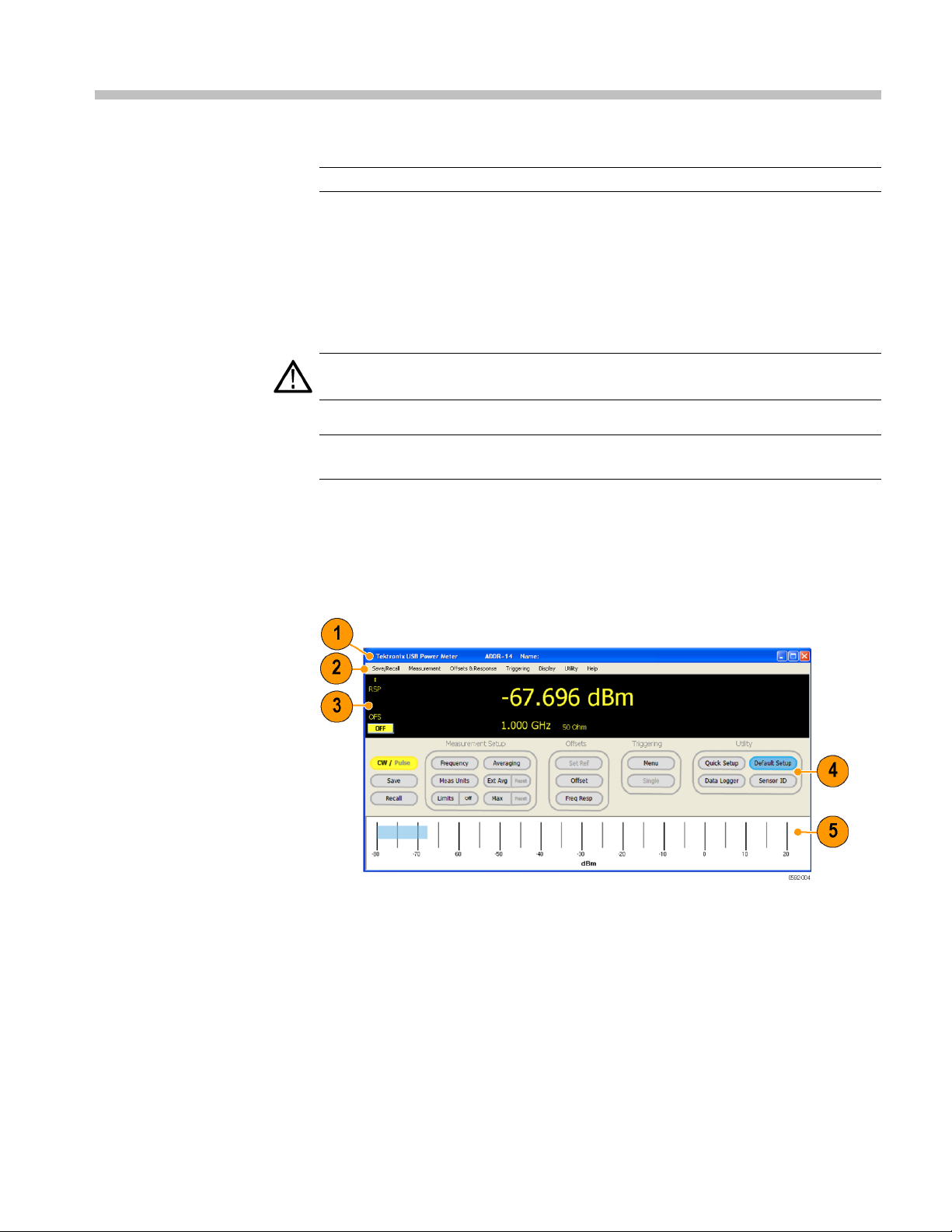
Figure 1: Power Meter application interface using a PSM5120
The main elements of the interface are:
1. Banner: the unit address and the unit name
2. Menus: drop down menus allow you to adjust various settings; many of these
settings are also accessible using the settings panel buttons
RF and Microwave Power Sensors/Met ers 19
Page 34

Power Meter Application
CW/Pulse
Save
Recall
3. Digital Readou
fail, low, high, or off
4. Settings Pane
utility functions by clicking on the related button
5. Power Meter
can be enabled in the Display drop down menu
Switch between CW and Pulse measurements.
Call the Sa
setup as a register or as a named state. This function is also accessible from the
Save/Recall drop down menu.
There are 10 Save/Recall registers and each register holds an entire state. The
states are not held in the instrument but reside on the local PC.
Call th
a state. This function is also accessible from the Save/Recall drop down menu.
ve Named State window. In this window, you can save your test
e Recall Named State window. In this window, you can recall a register or
t: shows measurements in digital format; shows limits as pass,
l: access measurement setups, offset setups, trigger setups and
Bar: provides an analog view of the meter reading; this view
Manage Named States
Frequency
Meas Units
Limits (On/Off)
This menu item is found in the Save/Recall drop down menu. It calls a Manage
Named
Select the frequency units (MHz or GHz). The center frequency must be updated
when the incoming signal frequency changes as this frequency setting is used
to d
frequency to be set and not doing so can be a significant source of error.
Yo
Select the power units (dBm, dBW, dBkW, dBuV, dBmV, dBV, W, V, dB Relative).
Set measurement limit specifications with pass or fail (High/Low) indicators
shown on the digital display panel.
From the Display drop down menu, you can establish a single test limit or upper
and lower test limits. Limits are fixed values against which a measured value
is compared. A n evaluation is done during a measurement and is expressed as
pass or fail.
For the single limit, the value can be below, equal to, or above this limit and you
may specify any of these conditions as pass or fail.
states window from which you can delete and view n amed states.
etermine calibration factors. The best measurement accuracy requires the
u can also find this item in the Measurement drop down menu.
20 RF and Microwave Power Sensors/Meters
Page 35

Power Meter Application
Averaging
For the upper an
between the limit, or equal to one of the limits. Any condition may be specified as
pass or fail.
Two t ypes of a
improve the stability of measurements, especially at low-levels: Averaging and
Extended Averaging.
The Averaging function averages some number of measurements and then
displays the averaged value. You can change the number of measurements that
are averaged from 1 to 100,000. By default, 75 measurements are averaged for
each displayed reading.
Averaging also has the effect of expanding the measurement interval. This
increases the amount of data used to determine peak pulse power, crest factor, and
duty cycle. For signals with narrow pulses or fast peaks, increase averaging to
e stable peak power, crest factor and duty cycle measurements.
achiev
For example, each raw measurement takes about 250 μs. Setting the averaging
000 would result in a 250 μs x 10,000 = 2.5 s delay between displayed
to 10,
readings. The average is calculated before each reading is displayed. If averaging
is set high, then the display updates slowly.
d lower limit, the value can be equal outside the limit, equal
veraging are available to use in the Power Meter application to
Extended Averaging /
Reset
Max / Reset
an combine Averaging and Extended Averaging to balance stability and
You c
responsiveness for your application and preference.
h the Ext Avg / Reset button and Measurement drop down m enu, you can set,
Wit
enable, and reset extended averaging. Extended averaging should be seen as an
adjunct to averaging: it may be used to further smooth readings and does not slow
down the display update rate as does averaging.
Since extended averaging applies a running exponential average of the last n
readings, where n is the number of extended averages, the display updates quickly
but the measurements respond to changes more slowly. The Reset button resets or
restarts both the max hold and extended averaging functions.
An xAvg indicator will appear in the digital display when extended averaging is
enabled and set greater than 1.
Retains the maximum measured value until reset or deactivated. For pulse
measurements, each reading (Pulse, Peak, CrF, Avg, DC) is held at its maximum
value independent of the other readings. You can reset or restart this function by
clicking on Reset. You can also find this item in the Measurement drop down
menu.
A MAX indicator will appear in the digital display when Max hold is enabled.
RF and Microwave Power Sensors/Met ers 21
Page 36

Power Meter Application
Set Ref
Offset
Freq Resp
Set the referen
to the power measurement on the display. When Ref Offset is activated, the REL
indicator will show in the digital readout display and the power units will change
to “dB relative”.
You can enable this setting from the Offsets & Response drop down menu item
called Relative Units On/Off.
Set gain or loss offsets to be applied to all measurements. You can also find this
item in the Offsets & Response drop down menu.
An OFS indicator will appear on the digital display when Offset is enabled.
Set frequency dependent gain or loss offsets to be applied to measurements. This
is a freq
response changes accordingly. Response amplitude is always expressed in dB
and the frequency is expressed in Hz. The interpolation is linear with respect to
frequency and dB. The frequency response feature must be enabled before it will
have an effect. A frequency response (RSP) indicator will appear on the digital
display readout when response correction is enabled.
The frequency response correction factors are specified as frequency and
amplitude pairs. To load the correction factors go to the Frequency Response
et window. Click Add after each frequency and offset entry to build the table.
Offs
Then select Show Graph to get a graphical presentation of the frequency offsets
that were entered in the table. The Response setup allows up to 201 points to be
entered.
ce value so that a subsequent power level can be measured relative
uency sensitive offset, so as you change the measurement frequency the
Anti-alias Control
Measured Pulse Setup
You can also find this item in the Offsets & Response drop down menu.
is function randomizes the sampling pattern to eliminate the effect of aliasing
Th
due to undersampling. The real-time sample rate of the instrument is 500 kS/s.
As the baseband signals approach the Nyquist criteria (about 200 kHz in this
case) anti-aliasing can occur. If you are measuring signals that have baseband
content greater than about 200 kHz, enable anti-aliasing for the best measurement
accuracy. Anti-aliasing slows down measurements, so for faster reading rates on
signals with modulation bandwidth below 200 kHz, disable anti-aliasing.
This function is found in the Measurement drop down menu.
This value determines the portion of the pulse to be used to measure pulse power.
The default or automatic value is 3 dB below the measured peak value or the
50% down points.
This function is found in the Measurement drop down menu.
22 RF and Microwave Power Sensors/Meters
Page 37
Power Meter Application
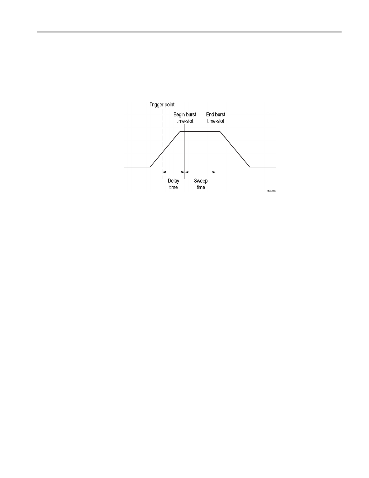
Burst Measurements
The PSM4000 and
on RF bursts. To access this measurement, select Burst Measurement... from the
Measurement drop down menu. From the window that appears, you can specify a
trigger, a delay relative to the trigger, and the sweep time over which the power
measurement is taken. The instrument will then display the peak power, average
power, and minimum power measured during the qualified duration.
Figure 2: Diagram of a burst time slot
Trigger. The measurement c an be triggered by the incoming RF signal, or from
an external TTL source. When using the Internal Auto Level setting, the trigger
level is automatically set to approximately half the pulse amplitude.
PSM5000 series instruments allow you to make measurements
Meas Update Rate
Delay. The delay time determines how long after the trigger the sweep time
begins.
Sweep Time. The sweep time defines the duration of the measurement.
Resolution. The power measurement data is taken at the real-time sample rate of
the instrument, which is 500 kS/s. This results in a fixed resolution of 2 μs.
Measure. The measurements consist of peak power, average power, and minimum
power observed during the specified sweep time. Measurements can be set to
update continuously by selecting the Continuous check box. Deselect the check
box to stop taking measurements. For a single set of measurements, click on the
Start button. The Copy button transfers the three measurements to the clipboard
so you can paste them into a document.
Data Logging. Burst measurements can be logged to a text file. To do this, type in
or browse to a file, and then enable logging by selecting the Log Measurements
check box.
The measurement update rate determines how quickly measurements are updated.
Options are S
This function is found in the Measurement drop down menu.
lowest, Slow, Medium, Fast, and Fastest.
RF and Microwave Power Sensors/Met ers 23
Page 38

Power Meter Application
Minimum Loss Pad
Menu (Triggering)
The instrument
a75Ω input impedance, you may attach a 75 Ω minimum loss pad (MLP) to the
input. You can correct for the pad by selecting 75 ohm MLP from the Offsets &
Response menu. The instrument will adjust its measurements accordingly and
the display will indicate “75ohm-MLP”, if selected.
This button calls the Triggering setup menu. From here you can set triggering to
internal or external continuous, and internal or external single. You can also set
the TTL trigger in/out, inverted trigger, and trigger timeout.
NOTE. When the trigger timeout is set to long and triggers occur slowly, the
Power Met
Trigger In. The external trigger input is assumed to be a TTL level and positive
edge tri
is detected, the measurement will commence and will continue for the specified
number of averages. In External Single mode, the system will wait for you to
click the Single button and then it will monitor the trigger in port. If a trigger is
not detected in the allotted time, the system will time out and return an ext trig?
indicator.
gger. Trigger in can be e nabled, disabled, or inverted. After the trigger
hasa50Ω input impedance. However, for applications requiring
er interface will respond slowly to mouse clicks.
Single
When the trigger in is inverted, the system will look for a negative edge (instead
of a positive edge) and begin the measurement when a negative edge is detected.
an set a trigger timeout period for an external trigger input, up to 30 seconds.
You c
Trigger Out. The trigger output is compatible with TTL levels. It can be enabled,
disabled, and inverted. A trigger out pulse occurs at the beginning of each
measurement. Even if the external trigger is disabled and trigger out is enabled, a
trigger will be produced each time a measurement is made.
By default, the trigger output is normally low. The start of the trigger is indicated
by a rising edge on the output. The output stays at a TTL high level for a few
icroseconds and then returns to a low level. If the trigger out is inverted, it will
m
transition from a high to a low TTL level to indicate when a trigger has occurred.
NOTE. When multiple Power Meter instances are running, the absence of a
trigger in one instance of the Power Meter application will cause other instances
to update at a slower rate or even time out. This would occur, for example, if an
instrument lost its external trigger source.
Enable this button from the Triggering drop down menu by selecting internal or
external single triggering. Click the button to initiate a single measurement.
24 RF and Microwave Power Sensors/Meters
Page 39

Power Meter Application
Quick Setup
Data Logger
Select to call a
window that allows you to set the mode (CW or Pulse), frequency,
power units, averages, and offsets all from one window.
You can also find this item in the Utility drop down menu.
This function allows you to plot measurement trends on the display or record a
measurement in a file. Use the Logging Setup menu item in the Measurement
drop down menu to set the following data logging options:
Turn off storage
Specify a file name
Settoappenddatatotheendofthefile
Set to overwrite data in a file
Click the Data Logger button to display the logging graph and start logging data
to a file once logging is set up.
The logger will start graphing from 0 to 300 readings (bottom scale, right to left).
The duty cycle is scaled v ertically from 0 to 10% (1% per divisio
n). Crest Factor
is scaled vertically from 0 to 20 dB (2 dB per division).
NOTE. There is a separate High Speed Logger application available for logging
high-speed measurements directly to a file. (See page 52, High Speed Logger
Application.)
Default Setup
Click this button to return all measurement parameters to their default settings,
but not user defined settings, such as display color or window size. When you
start the application for the first time, all parameters are in their d efault settings.
Unless you change one or more parameters, they will remain at their default
values. (See Table 2.)
Table 2: Power Meter default values
Parameter Default value
Mode
Frequency
Power units dBm
Averaging
Measured Pulse Setup 3 dB (PSM4000 and PSM5000 series only)
Measurement Update Rate Medium
Display
Sweep Time
Offset
CW
1GHz
75
Default
1ms
0 dB, disabled
RF and Microwave Power Sensors/Met ers 25
Page 40

Power Meter Application
Table 2: Power Meter default values (cont.)
Parameter Default value
Response 0 dB, disabled
Duty Cycle 10%, disabled
Minimum Loss Pad (75 ohm) Not selected. The Default Setup button will not
change the input impedance if this value is selected
(enabled). Application launch sets the input to 50 Ω.
Trigger Mode
Trigger Out
Internal Continuous
Disabled
Recall Factory Setup
Sensor ID
Set Address
Set Sensor Name
Select this menu item from the Utility drop down menu to reset all measurement
parameters and user preferences, such as display color and window size, to default
settings.
Click this button to identify an instrument. The LED on the identified instrument
will blink four times. This is particularly useful when multiple instruments are
connected.
You can als o find this item in the Utility drop down menu.
s item is located in the Utility drop down menu. Use it to set an instrument
Thi
address. This is particularly useful when multiple instruments are connected.
NOTE. Changing the address requires re-initialization of the USB connection.
After changing the instrument address, the application will close and must be
reopened.
This item is located in the Utility drop down menu. Use it to set an instrument
name for the current session only. This is particularly useful when multiple
instruments are connected.
Error Messages
Various error windows will appear if there is a hardware or software problem or
conflict. Follow the message instructions to correct the problem.
26 RF and Microwave Power Sensors/Meters
Page 41
Power Meter Application
Make an Averag
e Power (CW) Measurement
This example procedure applies to all instrument models and assumes a signal
source with the following parameters:
CW Frequency: 1 GHz
Power Level: 0dBM(1mW)
Modulation: off
RF Power: off
CAUTION. Do not exceed +23 dBm, 200 mW, or 3.15 VRMS.
1. For PSM4000 and P
on the Settings Panel to activate CW mode. Yo u can also enable CW from the
Measurement menu.
NOTE. For PSM3000 series instruments, the software is always in CW mode,
so the button is not available.
SM5000 series instruments, click the Pulse/CW button
2. Click Measur
will open.
3. Enter 1 GHz,
4. Confirm that the instrument is set to continuously trigger, and then click
Triggerin
5. Connect the instrument to the RF source and turn on RF power.
The display indicates approximately0dBmat1GHz. Thesoftwaretracks
changes as you vary the source power.
ement > Set Frequency and the Set Frequency dialog box
and click OK.
g > Internal Continuous.
RF and Microwave Power Sensors/Met ers 27
Page 42

Power Meter Application
MakeaPulseMe
asurement Using Duty Cycle
This method of measuring average pulse power is available with all instrument
models. However, this is the only method for measuring average pulse power on
PSM3000 seri
adjustment to the indicated power. This type of measurement is more prone to
error than the signal processing pulse power measurements available on PSM4000
and PSM5000 series instruments. However, this a useful measurement approach
when using PSM3000 series instruments.
The duty cycle correction calculation is:
Pulse Power = Measured Power + Duty Cycle Adjustment
The duty cycle adjustment is:
-(10log
For instance, if you measured an average power of -20 dBm and assumed a duty
cycle o
f 10% (0.10), then the pulse power would be calculated as:
Pulse Power = -20 dBm + -(10log
NOTE.
cycle measurement.
es instruments. This measurement uses an assumed duty cycle as an
(Duty Cycle))
10
The instrument must be in CW Power mode to access this method of duty
(Duty Cycle)) = -20 dBm + (10 dB) = -10dBm
10
t the instrument to measure average pulse power on a signal with 10% duty
To se
cycle, do the following:
1. For
PSM4000 and PSM5000 series instruments, click the Pulse/CW button
on the toolbar to activate CW mode. You can also enable CW from the
Measurement menu.
NOTE. For PSM3000 series instruments, the software is always in CW mode,
so the button is not available.
2. Click Offsets&Response>DutyCycle>Setup.
The Measurement Duty Cycle dialog box opens.
3. Enter 10.0 (the duty cycle percentage), and click OK.
4. Click Offsets & Response > Dut y Cycle > Enabled.
The software shows source pulse power in the CW configuration, and the
DC annunciator activates. You can use the duty cycle pulse power method
down to approximately 0.1%.
28 RF and Microwave Power Sensors/Meters
Page 43

Make a Pulse Power Measurement
This example procedure applies to the PSM4000 and PSM5000 series instruments
only. It assumes an RF signal source for a pulse-modulated output with the
following parameters:
CW Frequency: 1 GHz
Power Level: 0dBM(1mW)
PRF: 10 kHz (or a PRI of 0.1 ms)
Power Meter Application
Pulse Modu
RF Power: off
CAUTION.
1. Click Measurement > Pulse Power.
Or, click the Pulse/CW button o n the toolbar to activate Pulse mode.
2. Click Measurement > Set Frequency.
The Set Frequency dialog box opens.
3. Enter 1 GHz, a
4. Confirm that the instrument is set to continuously trigger, and then click
Triggering
In Pulse Power mode, the software shows these measurements at the right of
the displa
DC: duty cycle
lation: 50% Duty Cycle (or a pulse width of 50 μs)
Do not exceed + 23 dBm, 200 mW, or 3.15 VRMS.
nd click OK.
> Internal Continuous.
y:
Pk: peak power
Avg: average power
CrF: crest factor (also known a s peak-to-average power ratio (PAR))
The large number in the center of the software display shows the pulse
power. The default pulse threshold is Automatic 50% or 3 dB below peak
check box in the Pulse Setup dialog box (Measurement > Measured
Pulse Setup). If you know the s pecifi c pulse characteristics, you can
change this by selecting Measured Pulse Setup in the Measurement drop
down m
RF and Microwave Power Sensors/Met ers 29
enu.
Page 44

Power Meter Application
5. Connect the ins
The software should indicate these approximate values:
1 GHz
0 dBm pulse power
50% duty cycle
0dBmpeak
-3 dBm aver
3 dB crest factor (the ratio between peak and average power)
The measurement changes as you vary the source power.
trument to the RF source and turn on RF power.
age
30 RF and Microwave Power Sensors/Meters
Page 45

Pulse Profiling Application
Pulse Profilin
Menu Features
gApplication
NOTE. This application is only available for PSM5000 series instruments.
For basic CW
To perform detailed measurements on repetitive, pulsed RF and microwave
signals with PSM5000 series instruments, use the Pulse Profiling application.
This application displays a trace of the pulse envelope and allows you to take
measurements at any point on the trace.
CAUTION. Do not exceed +23 dBm, 200 mW, or 3.15 VRMS. Ensure that the RF
input co
NOTE. Using more than one type of application at a time can result in errors. It is
recomm
ThemainelementsofthePulseProfiling application interface are shown here.
and pulse power measureme nts, use the Power Meter application.
nnector on the sensor and the mating connector are clean and undamaged.
ended that you use only one type of application at a time.
Figure 3: Pulse Profiling application interface
RF and Microwave Power Sensors/Met ers 31
Page 46

Pulse Profiling Application
Highlight Span
The main elemen
1. Banner: unit address and the unit name
2. Toolbar: Allows you to configure the instrument for measurements, control
the display, access Help, and perform other tasks. (See page 36, Toolbar
Functions.)
3. Panoramic Trace: The Panoramic Trace is displayed on a grid with 10 vertical
divisions that indicate power, and 10 horizontal divisions that indicate time.
You can highlight a portion of the Panoramic trace by clicking and dragging
the cursor directly on the Panoramic trace. Current tra ce parameters are also
listed above the grid.
4. Measurement Trace: The highlighted time segment from the panoramic trace
will appear in this view, allowing for a more detailed examination of the
signal using time markers and time gates. The Measurement trace is displayed
on a grid with 10 vertical divisions that indicate power, and 10 horizontal
divisions that indicate time.
5. Auto Measure Panel (Results and Auto Measure windows): This panel
contains the Auto Measure and Results windows and a display control toolbar.
(See page 34, Auto Measure Panel.)
The Panoramic Trace and the Measurement Trace windows are designed to work
in tandem to help you identify a nd investigate areas of interest easily and q uickly.
To view a portion of the Panoramic trace in more detail, highlight the portion of
the trace in which you are interested. The highlighted portion will appear in the
Measurement Trace window.
ts of the display are:
You can highlight or select a portion of the trace using the following techniques:
1. Click and drag the mouse over a portion of the Panoramic trace. Only the
portion selected by the mouse movement will be viewed in the Measurement
Trace window .
2. Click and drag the mouse over a portion of t he Measurement trace. Only the
portion selected by the mouse movement will be viewed in the Measurement
Trace window. This technique allows you to zoom in on the trace. The mouse
pointer must be in Highlight mode.
3. Click the Highlight Span drop down on the Results pane (or Display Control
toolbar) and then select the percentage of interest. The selected portion will
be viewable in the Measurement Trace window. If a portion of the Panoramic
trace is currently selected, then the percentage will be centered on the current
selection. If a portion of the trace is not selected, then the percentage will be
centered around the middle of the Panoramic trace.
4. To select a precise portion of the trace, click the Highlight Span drop down
and then select Set Start. Enter the beginning of the measurement trace in
microseconds.
32 RF and Microwave Power Sensors/Meters
Page 47

Pulse Profiling Application
CDF, CCDF, and PDF
Display
5. Click the Zoom I
current viewing area. These buttons are available in the Results window and
in the Display Control toolbar.
6. Click the Reset button. This resets the Measurement Trace window to include
the entire Panoramic trace.
7. Use the scroll and nudge controls in the Results window. These controls allow
you to scroll the area of interest left or right. The nudge controls move the
area one small step at a time.
You can select to print CDF (Cumulative Distribution Function), CCDF
(Complementary Cumulative Distribution Function), or PDF (Probability Density
Function) displays from the Print toolbar. All displays are printable in black and
white or color (depending on the capabilities of your printer). For all of these
displays, you can set the resolution, data source (trace or gates), minimum and
maximum
Pulse Profiling.)
The CDF
level.
The CC
average power level (expressed in dB relative to the avera ge power). The
percentage of time the signal spends at or above each line defines the probability
for that particular power level. A CCDF curve is a plot of relative power levels
versus probability.
power, and the number of data sets or runs with counter. (See page 16,
display shows the probability that a signal is below the average power
DF display shows how much time the signal spends at or above the
n or Zoom Out buttons. These buttons double or halve the
Power (CCDF) curves provide critical information about the signals encountered
in 3G systems. These c urves also provide the peak-to-average power (crest factor)
data needed by component designers.
The PDF shows the distribution of the average power level.
NOTE. Read more about the Print toolbar. (See page 46, Print.)
RF and Microwave Power Sensors/Met ers 33
Page 48

Pulse Profiling Application
Auto Measure Panel
The Auto Measur
window. Click the Start Measurement button to start the automatic measurement
feature and get a complete characterization of the pulse based on the selected
sweep time.
Results Window. This window allows you to set up markers and ga tes for specific
measuremen
values, marker values, and gate values.
e panel consists of the Results window and the Auto Measure
ts. It also shows the measurement values that include current trace
34 RF and Microwave Power Sensors/Meters
Page 49

Pulse Profiling Application
Auto Measure Wi
of measurements based on the Measurement Trace window by clicking the
Start Measurement button. A toolbar also allows you to select Gates, Markers,
or Highlight functions; to select the percentage of h ighlight; to reset the
Measurement Trace window to include the entire Panoramic trace; and to zoom
in and out on the Measurement trace.
In addition to the gate measurements, the Auto Measurement feature performs
an On/Off Ratio measurement. This measurement returns the difference in dB
between th
pulse is off during the first complete cycle.
ndow. This window allows you to make a comprehensive list
e average power while the pulse is on to the average power while the
NOTE. The Auto Measurement feature requires at least two complete cycles of
the pulse to be viewable in the Measurement Trace window in order to make
accurate measurements.
Start Measurement. Click Start Measurement to capture the instantaneous
values shown above. The readings will not continuously update, but will make a
single sweep of the trace. You must click Start Measurement each time to update
the measured readings. A description of each measurement is shown at the bottom
of the pane when you click on the measurement label.
Copy Data. Click Copy Data to copy the measurement results to the clipboard
and then paste it to your document of choice.
RF and Microwave Power Sensors/Met ers 35
Page 50
Pulse Profiling Application
Customize the Display
The display is c
display using Microsoft drag and drop tools.
Moving menu tabs. You can rearrange the menus in the menu p anel. Just click
on the menu you want to move and then drag it the desired location in the menu
panel. When you release the mouse button, the menu will be in the new location.
Moving windows. The Panoramic Trace, Measurement Trace, Results, and Auto
Measure windows can be moved and placed anywhere on the display using the
docking popup or by clicking and dragging.
To activate the docking popup and move a window, do the following:
1. Click and hold on one of the four windows in the display.
2. Drag the window until you see the docking popup appear.
3. Place the window you are moving over one of the positions (top, bottom,
center, right, left) on the popup. This position represents how the window will
be docked on the display and that area of the display will become highlighted.
NOTE. You can also place a window anywhere on the display without using the
docking popup. Simply click and drag the window to the desired location and
then release the mouse button.
omposed of five movable windows that can be rearranged on the
Toolbar Functions
Main
4. Release the mouse button and the move will be completed.
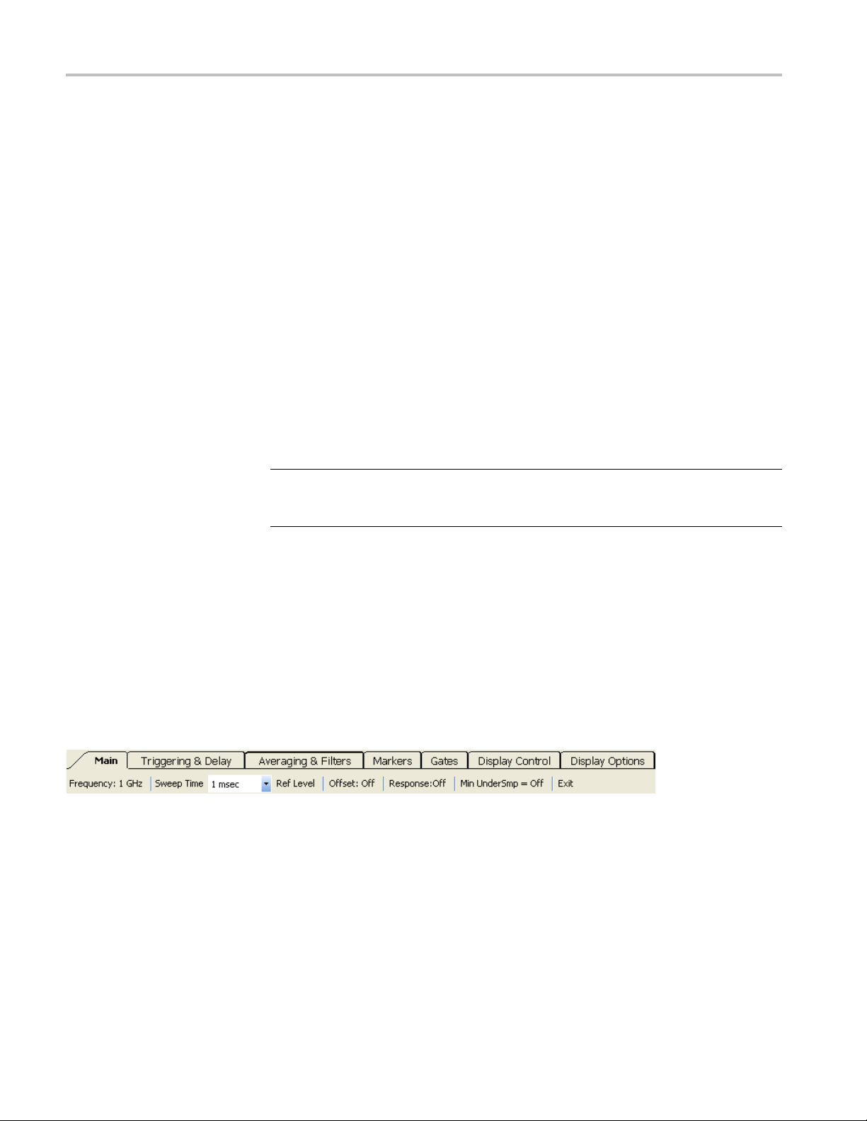
The toolbar functions allow you to set the following parameters.
The Main toolbar allows setting of the measurement Frequency; Sweep Time;
Reference Level and Resolution; Offset and (frequency) Response.
Frequency. The frequency setting must match the signal carrier frequency to
achieve the most accurate measurements. Setting the frequency is essential to
making accurate measurements because readings are corrected based on frequency
(calibration factors). Significant errors can occur if you do not set the frequency
properly, especially at the upper end of the frequency range.
Sweep Time. The following table shows the relationship between sweep time,
sample rate, and total number of samples. Notice that the resolution of most
computer displays is limited to somewhere between 1000 and 2000 points.
36 RF and Microwave Power Sensors/Meters
Page 51

Pulse Profiling Application
However, the tr
ace data has much higher resolution. If you want to see more
detail on a 10,000 point trace, for example, you can use the zoom icons on the
Display Control toolbar. (See page 44, Zoom In and Out.)
Table 3: Sweep time values
Sweep time Time between samples Length of trace
10 μs 0.0208 μs 480 points
20 μs 0.0208 μs 960 points
50 μs 0.0208 μs 2400 points
100 μs 0.0208 μs 4800 points
200 μs 0.0208 μs 9600 points
500 μs0.05μs 10,000 points
1ms 0.1μs 10,000 points
2ms 0.2μs 10,000 points
5ms
10 ms 1.0 μs 10,000 points
20 ms 2.0 μs 10,000 points
50 ms 5.0 μs 10,000 points
100 ms 10.0 μs 10,000 points
200 ms 20.0 μs 10,000 points
500 ms 50.0 μs 10,000 points
1 s 100.0 μs 10,000 points
0.5 μs 10,000 points
Reference Level. The Reference Level allows you to change the maximum value
displayed in the Panoramic and Measurement windows. It also allows you to
change the vertical scale in the Measurement window.
The vertical scale setting only applies to the Measurement window.
NOTE. The reference level and resolution settings are display functions that
change the formatting of the data that is presented, whereas offset and response
modify the measured values.
Offset. This function applies a constant offset to all measured data. It shifts the
actual values of the measured data. Simple offsets can be useful, but they are
limited in that they are not sensitive to frequency. If there is a frequency sensitive
device in the measurement path, then every frequency change requires a change in
offset. In this case, the Response function may be more appropriate.
The Offset function must be enabled to affect measurements. The Offset
annunciator is visible above and to the right of the measurement trace when the
Offset function is enabled.
RF and Microwave Power Sensors/Met ers 37
Page 52

Pulse Profiling Application
Response. Use t
devices like directional couplers. The Response function allows you to enter a set
of amplitude and frequency pairs. As you change the frequency of measurement,
the application automatically adjusts the offset based on the frequency you
selected.
The Response function must be enabled to affect measurements. The Response
annunciator is visible above and to the right of the measurement trace when the
Response function is enabled.
Minimize Undersampling. For sweep times of 10 ms or less, equivalent-time
sampling (undersampling) is used to provide adequate time resolution and fill
the trace memory. The Minimize Undersampling function has no effect at these
sweep time settings.
For sweep times of 20 ms, 50 ms, and 100 ms, undersampling provides more
samples than are needed to fill the trace memory. When Minimize Undersampling
is turned off, samples are averaged together to fit into the 10,000 point trace. When
the Minimize Undersampling function is turned on, equivalent-time samples that
do not fit into the trace are not averaged, but are discarded. Activating this function
will tend to increase the noise on the trace, but it improves the ability to see peaks.
For sweep times of 200 ms or more, real-time sampling provides enough samples
to fill the trace memory and to give adequate time resolution. Undersampling is
not used and the Minimize Undersampling function has no effect at these sweep
settings.
he Response function for correcting measurements through
Triggering & Delay
NOTE. You can read more about sweep time values. (See Table 3.)
Exit. Select to exit the application.
The Triggering and Delay toolbar allows you to set trigger and delay parameters.
Trigger Source. You have three options for trigger source settings. All of
these options allow you to use positive or negative Edge triggering, as well as
Continuous or Single Sweep.
Internal Auto Level: The trigger is based on the input signal. As the input varies,
the auto trigger level will be adjusted accordingly. This trigger mode always
returns a trace. A trigger pulse is sent out the TTL trigger output each time a
sweep starts. If a signal is not present, then it will return a noise trace. This trigger
source is not recommended when peak input levels fall below approximately
-50 dBm. In these cases, use Internal Manual Level.
38 RF and Microwave Power Sensors/Meters
Page 53

Pulse Profiling Application
Internal Manua
based on the input signal as it crosses the level you s pecify. If you set the trigger
level too high, then you will not get a trace. Instead, you will get a “Trigger?”
message in the middle top of the Mea surement grid. This message indicates that a
trigger was not found. If the trigger is set too low, then the system will trigger on
noise. A trigger pulse is sent out the TTL trigger output each time a sweep starts.
External TTL: The instrument will take a measurement after it senses a transition
on the TTL trigger input (TI). To use this trigger function, connect an SMB
cable to a TTL trigger source. Use this capability to trigger on very low signal
levels approaching the noise floor of the instrument. For measuring very low
signal levels, use the Averagi
Filters.)
NOTE. An incoming pulse for an external TTL trigger must be on at least 0.20 μs
followed by at least 1 μs of off time for the sensor to properly trigger.
Trigger Level. Usethismenufunctiontosetthetrigger level when the trigger
source is set to Internal Manual Level.
Edge. Use this menu function to set the instrument to trigger on a positive or
negative edge.
l Level: You must set the trigger level manually. The trigger is
ng and Filters functions. (See page 40, Averaging &
Continuous. Use this menu function to set the instrument to continuously provide
a new trace with each new trigger event.
Single Sweep. Use this menu function to set the instrument for a single sweep.
The instrument will then wait for a trigger each time the Single button is clicked.
Single. This button is blue when Single Sweep trigger is active. Click this button
to initiate a trigger sequence.
Delay Trigger. Use this menu function to delay the beginning of a trace
triggereventforupto10ms. Thismaybeusedtocapturehighresolutiontraces
long after the trigger e vent.
Trigger Out. Use this menu function to enable the TTL trigger output (TO) signal
and invert it.
Timeout. Use this menu function to set a timeout period for an external trigger
input (up to 10 seconds). If a trigger event is not detected in the allotted time, the
system will time out and the Tr igge r? indicator w ill appear at the top center of
the Measurement Trace window.
NOTE. If the trigger timeout is set long, and triggers occur slowly, the meter
display will appear sluggish as the instrument waits for triggers.
from the
RF and Microwave Power Sensors/Met ers 39
Page 54
Pulse Profiling Application
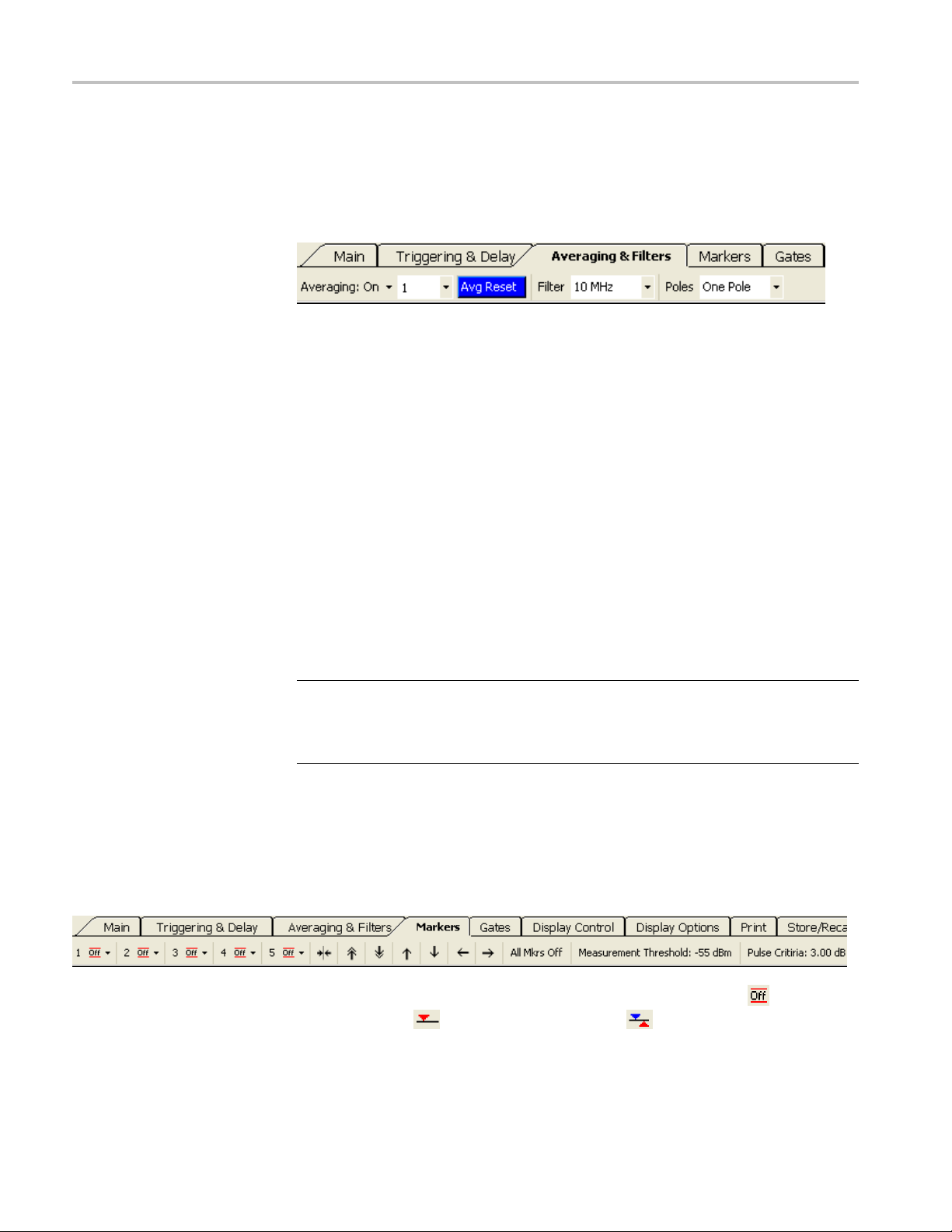
Averaging & Filters
You can use aver
near the noise floor of the instrument. Increasing the number of averages
maintainswaveshapebutslowsdowntheupdaterateofthetrace. Alower
low-pass filter setting will provide faster trace updates, but results in a rounded
pulse shape with longer rise and fall times.
Averaging. Select to turn averaging on or off. When this function is turned on,
you can s elect the number of traces to be averaged from the drop down m enu. The
number of averages c an be set from 1 to 100. It takes 0.3 to 1.0 ms to collect
each trace.
Average Reset. This button is blue when averaging is turned on. Click the button
to restart or reset trace averaging.
Filter. This function allows you to select an appropriate low-pass video filter
depending on your measurement needs. You can choose 100 kHz, 200 kHz,
300 kHz, 500 kHz, 1 MHz, 2 MHz, 3 MHz, 5 MHz, and 10 MHz. (The 10 MHz
setting is equivalent to turning the filter function off.)
Poles. This menu selection allows you to choosefromone,two,three,orfour
poles. The number of poles determines the roll off rate of the low pass video filter.
The greater the number of poles, the steeper the roll off, resulting in a reduction in
the high frequency components of the signal.
aging and the low-pass filter can help improve measurements
Markers
NOTE. An informational dialog box will appear if the measurement becomes
uncalibrated due to filter, poles, or sweep time settings. An “Uncal Meas” label
will also appear on both the Panoramic Trace and Measurement Trace grids.
Adjust the settings accordingly until the error message stops.
Markers are used to make measurements at a particular point (Normal Markers) or
measure the difference between two points (Delta Markers). Markers are only
available in the Measurement Trace window. The value of the active marker is
displayed in the upper left portion of the Measurement Trace window unless it is
turned off. The value of each marker is d isplayed in the Results window.
Marker 1 through 5. Select the marker numbers to turn them off ( ), on as a
Normal marker (
Position from each marker drop down menu to position the marker. You can also
place the marker by clicking in the Panoramic Trace window.
), or on as a Delta marker ( ). You can then select Set
40 RF and Microwave Power Sensors/Meters
Page 55

Pulse Profiling Application
To move or place
Display Control toolbar and in the Results window) must be set to Markers
(
Once a marker is turned on and the pointer mode is set to Markers, you can click
and drag on the Measurement area to position the marker. As you move the
marker, the notation in the upper left corner of the Measurement grid will be
updated. The x value (time) is determined by the position of the cursor. The
y value (magnitude) is determined by the value of the trace closest to that point
in time.
NOTE. Only one marker can be active at a time, although all five markers can
be displayed simultaneously. The active marker will have an asterisk (*) next to
its number in the toolbar and the marker number will be underlined and appear
slightly larger in the trace display.
ANormalMarker( ) is a single data point and appears above the Measurement
trace.
A Delta Marker (
Measurement trace. To use a Delta marker, do the following:
).
a particular marker, the Pointer Control mode (found in the
) gives the differential value and appears below the
NOTE. There is a procedure in this document for making a meas
markers. (See page 48, Make a Marker Measurement.)
Arrow Icons. The arrow icons allow you to position the mark
first arrow icon allows you to center the highlight trace on a marker.
All Mrkrs Off. Select to turn off and reset all markers. You will lose marker
positioning if you click this button.
Measurement Threshold. Select to view the Threshold window where you can set
the threshold value, e nable the threshold, or return the threshold to a default value.
The measurement threshold sets the minimum value of the peaks considered by
the marker and gate search algorithms. It is adjustable across the limits of the
dynamic range of the instrument. The default setting is -55 dBm and the function
must be enabled/disabled from the dialog box.
NOTE. The Measurement Threshold function is also used to set the lower limit
of data used in gated measurements.
Pulse Criteria. Select to view the Pulse window where you can set the threshold
value, enable the threshold, or return the threshold to a default value. This
function is used to define that portion of the total trace that is to be considered
urement using
ers on a peak. The
RF and Microwave Power Sensors/Met ers 41
Page 56

Pulse Profiling Application
Gates
part of a pulse.
entire pulse and is relative (or added) to the measurement threshold if threshold is
enabled. It is relative to the noise floor if the measurement threshold is disabled.
The time gate
and droop measurements are very sensitive to the position of the gates. These
measurements use the position of the gates as starting and end points for the
measurement. (See page 42, Gate Measurement Types in Gates Toolbar.)
Gates A through E. There are five time gate pairs (A-E). The drop down menu for
each gate allows you to set measurement type and gate position.
You can then select Set Position from the gate drop down menu to access the Set
Position window to place the gate. You can also place the gate by clicking in
the Panoramic Trace window.
To move or place a particular gate, the Pointer Control mode (found in the Display
Control toolbar and in the Results window) must be set to Gates (
Thepulsecriteriadefines the edges of the positive portion of the
s allow you to characterize the incoming signal. Rise time, fall time,
).
te Measurement Types
Ga
in Gates Toolbar
NOTE. Only one gate can be active at a time, though all five gates can be
displayed simultaneously. The active gate will have an asterisk (*) next to its
letter in the toolbar and the gate letter will be underlined and appear slightly
larger in the trace display.
The following general gate positioning diagram shows where to place the gates
for the various measurement types. (See Figure 4.)
The time gates allow characterization of the pulse signal to include the following
parameters, selectable in the Gates toolbar from the Gate drop down menus. You
can also make all of the following measurements automatically by clicking the
tart Measurement button in the Auto Measure window.
S
A brief description of every measurement follows. After the list of measurements,
there are some measurement examples that guide you through the gate setups.
Rise Time (RT). Returns the time required for the signal to increase in amplitude
from 10% to 90% of the amplitude defined by the placement if the right-most gate.
RT is measured on the first complete pulse: the left gate determines the start of
data and the right gate marks the highest point to b e considered.
42 RF and Microwave Power Sensors/Meters
Page 57

Pulse Profiling Application
Fall Time (FT).
from 90% to 10% of the amplitude as defined by the placement of the left-most
gate. The right gate defines the end of data for this measurement.
Pulse Width (PW). Returns the pulse width in μs. The width of the pulse is the
time for a signal to rise to within 3 dB of the top of the pulse, and then fall 3 dB
below the top of the pulse. The left-most gate defines the start of data and must
precede a positive going edge. The right-most gate defines the end of data and
must follow o ne or more subsequent falling e dges.
Pulse Repetition Time (PRT). Returns the PRT in μs. The PRT is the time between
the first rising edge and the second rising edge. The gates for this measurement
must include at least one complete, uninterrupted cycle. The left-most gate must
follow a positive going edge and the right-most gate must precede one or more
subsequent falling edges and at least one rising edge.
Pulse Repetition Frequency (PRF). ReturnsthePRFinHzorkHz.ThePRFisthe
inverse of the time (1/PRT) between the rising edges of two successive pulses.
The pulse edges are defined by the pulse peak criteria. This measurement can be
limited by the threshold value. The gates for this type of measurement must be
positioned with the same restrictions as the PRT measurement.
Duty Cycle (DC). Returns the percentage of on time during a selected cycle. The
gates for a duty cycle measurement m ust be positioned with the same restrictions
as the PRT and PRF measurements. The measurement then proceeds to sort all
samples into one of two bins. One bin is the “ON” bin and the other bin is the
“OFF” bin. All points within 3 dB of the pulse top are placed in the “ON” bin. All
other samples are placed in the “OFF” bin. Then a simple c alculation is done:
Returns the time required for the signal to decrease in amplitude
DC (Duty Cycle) = #ON samples / (#ON samples + #OFF samples)
Pulse Power (Pls). Returns the average power between the rising and falling
edges of the first complete pulses in dBm. The gate must be positioned exactly
like PW measurements. The average of all samples between the rising and falling
edges is reported. The pulse edges are defined by the pulse peak criteria. This
measurement can be limited by the threshold value.
ak Power (Pk). Returns the highest power level between two gates. There is
Pe
no requirement for a rising or falling edge anywhere within the measurement
window as defined by the gates.
Average Power (Avg). Returns the avera ge power between two gates. There is
no requirement for a rising or falling edge anywhere within the measurement
window as defined by the gates.
Crest Factor (CF or CrF). Returns the difference between the peak power and
average power in dB. There is no requirement for a rising or falling edge anywhere
within the measurement window as defined by the gates.
RF and Microwave Power Sensors/Met ers 43
Page 58

Pulse Profiling Application
Overshoot (OvS
a rising edge and the average power of the pulse. The gates for this type of
measurement must be positioned with the same restrictions as the rise time
measurement.
Droop (Droop). Returns in dB a decrease in pulse power measured between the
first 5% afte
The gates also provide the following three groups of measurements:
Power Set : peak power, pulse power and crest factor
Time & Frequency Set: pulse width, pulse repetition time, pulse repetition
frequency
Mixed Set: peak power, crest factor, pulse width, pulse repetition frequency
Below is a general gate positioning diagram that shows where to place the gates
for the various measurement types.
h). Returns the difference in dB between the highest point after
r the left gate and the last 5% before the right gate.
Figure 4: Gate positioning diagram
All Gates Off. Select to turn off and reset all gates. You will lose gate positioning
if you click this button.
Display Control
44 RF and Microwave Power Sensors/Meters
This toolbar allows you to adjust the trace display views and switch control of the
mouse pointer function between Markers, Highlight, or Gates.
Zoom In and Out. Click the zoom icons to increase or decrease the trace display
resolution. These icons are also available at the top of the Results window.
Page 59

Pulse Profiling Application
Display Opt
ions
Reset. This but
available at the top of the Results window.
Pointer Contr
Markers (
mouse can man
These icons are also available at the top of the Results window.
This toolbar allows you to adjust how the trace windows and other windows are
viewed. For example, you can adjust the size and color of markers and gates in
the Measur
Marker Color and Size. This button allows you to change the style (shape), color,
and size
and make your selections.
of the markers. Click to button to view the Marker Definition window
ton returns the Measurement trace to full view. This option is also
ol. The Pointer Control mode can be set to Highlight (
), or Gates ( ). The settings control which of these the
ipulate when clicking and dragging in a trace display.
ement Trace window or the appearance of text in the Results window.
),
RF and Microwave Power Sensors/Met ers 45
Page 60

Pulse Profiling Application
Gate Color and S
and size of the gates. Click to button to view the Gate Definition window and
make your selections.
Display Font. This button allows y
language (script) of the trace display text.
ize. This button allows you to change the line style, color,
ou to change the font type, style, size, and
Print
Display Colors. This button allows you to select the background, trace, grid, text
and notation, and highlight colors from a drop down menu. You can also select
the degree of highlight opacity.
Themes. This button allows you to select color themes for the display from a
drop down menu.
Grid On/Off. This button allows you to turn the Panoramic and Measurement
Trace window grids on and off.
Meas Notation On/Off. This button allows you to turn the measurement notation in
the Panoramic and Measurement Trace windows on and off.
This toolbar enables you to select to print the Panoramic trace and the
Measurement trace. You can also select to print CDF (Cumulative Distribution
Function), CCDF (Complementary Cumulative Distribution Function), or PDF
(Probability Density Function) displays. All displays are printable in black and
white or color (depending on the capabilities of your printer). (See page 33, CDF,
CCDF, and PDF Display.)
46 RF and Microwave Power Sensors/Meters
Page 61

Pulse Profiling Application
Store/Recall
Utility
This toolbar en
Store Register. This button allows you to store a register. A register holds an
entire stat
Recall Register. This button allows you to recall a stored register. A register
holds an entire state
StoreasName. This button allows you to store the current setup state.
Recall as Name. This button allows you to recall a stored named register or file.
Copy Trace Data. This button allows you to paste the trace data as time and
amplitude pairs into other applications, like Excel, for further analysis.
This toolbar enables you to set the instrument address and verify instrument ID. It
also allows you to perform two types of reset: default setup and factory recall.
Read more about the differences between these two options below.
ables you to store and recall measurement states.
e.
Default Setup. Click t his button to reset measurement parameters only. Any
display changes, such as colors and fonts, will not be affected when you select this
default option. (See Table 2.)
nsor ID. Click this button to make the instrument associated with this
Se
application session identify itself. The green LED on the related instrument
will blink four times. This is particularly useful when multiple instruments are
connected to a computer.
RF and Microwave Power Sensors/Met ers 47
Page 62

Pulse Profiling Application
Help
Set Address. Cl
useful when multiple instruments are connected to a computer.
Recall Factory Setup. Click this button to reset all measurement parameters and
user preferences, such as display colors and fonts, to default settings.
The Help drop down menu provides access to a help document for this application
and a link to the Tektronix Web site to download user manuals. Click About to
view software, firmware, and driver version information.
ick this button to set the instrument address. This is particularly
Make a Marker Measurement
Pulse width measurements are normally defined as the time between the 3 dB
points on the rising and falling edges of a pulse. When using markers for a
measurement like this, the results are highly dependent on the placement of the
kers. Placing markers at the precise 3 dB down points can be problematic for
mar
pulses with very fast rise and fall times.
llow this procedure to make a marker measurement of a pulse width:
Fo
1. Highlight a single pulse in the Measurement Trace window. (See page 32,
ighlight Span.)
H
2. Zoom in on the pulse to position the marker for a Pulse Width measurement.
3. Select Markers from the toolbar.
4. ClickontheMarker 1 down arrow and select the Normal marker type.
Notice that Marker 1 appears in the Measurement window at center graticule.
48 RF and Microwave Power Sensors/Meters
Page 63

Pulse Profiling Application
The mode in the Results window toolbar will switch from highlight ( )to
Markers (
NOTE. Alternately, you can right-click on the individual marker in the Results
window to sel
5. Move the marker to the left edge of the pulse. The delta will be measured
relative to
6. ClickontheMarker 2 down arrow and select the Delta marker type. Notice
that Marke
7. Place the Delta marker at the right edge of the pulse.
8. Notice that the Delta Marker 1 (DMk1) value located above the left edge
of the Measurement grid is the approximate pulse width of the signal. The
relativ
9. Click All Mkrs Off to turn off the markers when you are finished.
ect the marker type.
e and absolute Delta marker values are shown in the Results window.
) in the Results window.
this value.
r 2 appears in the Measurement window at center graticule.
Make a Gated Measurement
Follow this procedure to set up the gates b ased on the example input used for
marke
1. Highlight a single pulse in the Panoramic window. (See page 32, Highlight
Span
2. Click the zoom in icon in the Results window and scroll left or right to center
the
3. Select the Gates toolbar.
4. All gates (A-E) should be off. Left-click on the Gate A drop down menu and
select Pulse Width.
5. Observe that the gate pair appears at center graticule in the Measurement
window. The active gate will have an asterisk (*) next to it in the toolbar
a
Trace window.
6. Observe that the measured value will appear in the Results window under the
active gate and above the grid in the Measurement window.
rs.
.)
pulse.
nd the A will be underlined and appear slightly larger in the Measurement
RF and Microwave Power Sensors/Met ers 49
Page 64

Pulse Profiling Application
7. Pulse width mea
3 dB points. Do the following to adjust the gates:
NOTE. A complete cycle of the incoming signal must be gated for periodic
measurements such as duty cycle and frequency.
a. Click on the left gate in the Measurement window and move it to the
left until the rising edge of the pulse is p ositioned to the right of the left
gate. (See Figure 5.)
b. Click on the right gate in the Measurement window and move it to the
right until the falling edge of the pulse is positioned to the left of the right
gate. (See Figure 5.)
surements require a rising and falling transition through the
50 RF and Microwave Power Sensors/Meters
Page 65

Pulse Profiling Application
8. Observe that th
pulse is selected. That is, if you move the left gate closer to the left edge of
the display, the measurement result remains unchanged.
e measurement result does not change as long as an entire
Figure 5: Position of gates for measurement
9. Observe that the drop down menu on each gate shows the selection of
measurements that can be made. You can also right-click on the gate in
the Results window. A dashed line (–.–) will appear if the gate cannot take
a measurement or is not set.
You can compare a manual measurement like the one just explained with an
automatic measurement by doing the following:
1. Check that there are at least two pulse cycles in the Measurement window.
2. Click on the Auto Measure tab to view the Auto Measure window.
3. Click Start Measurement.
4. Compare the results.
RF and Microwave Power Sensors/Met ers 51
Page 66
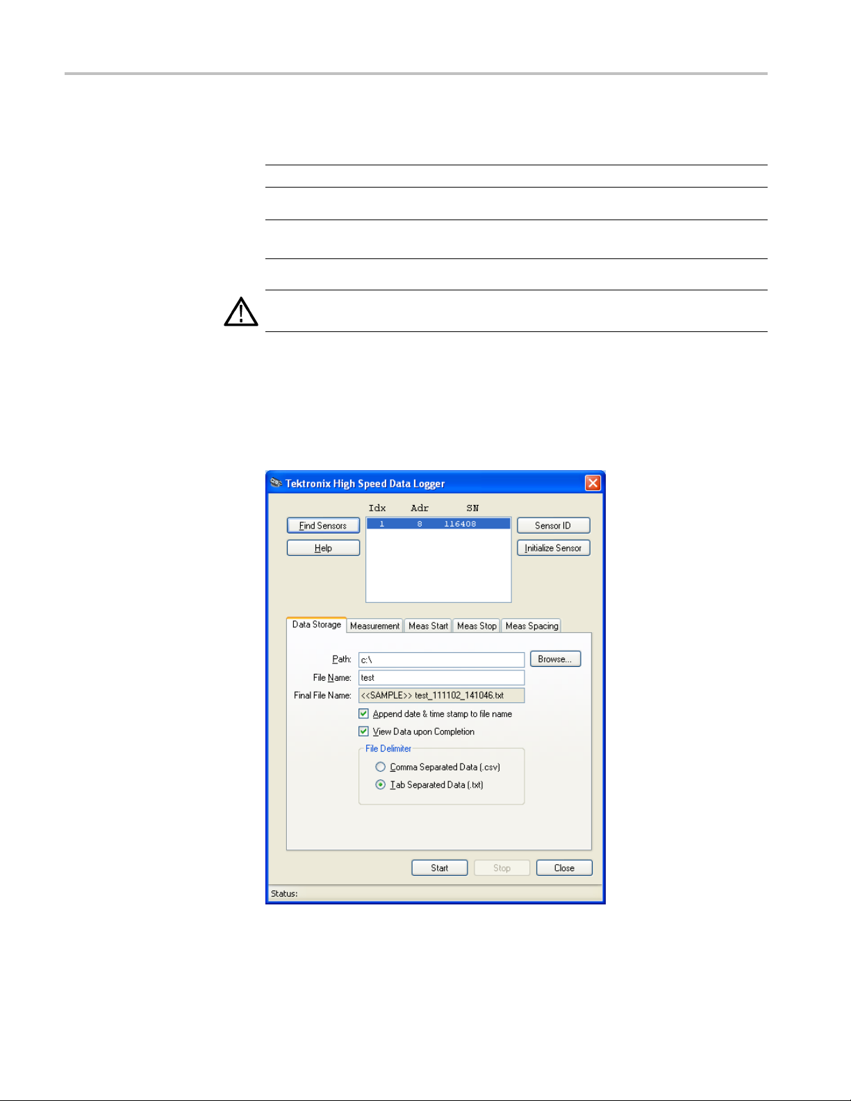
High Speed Logger Application
High Speed Log
ger Application
NOTE. This application is available for all instrument models.
NOTE. Using
recommended that you u se only one type of application at a time.
CAUTION. D
input connector on the sensor and the mating connector are clean and undamaged.
When you
asking if you would like to initialize the instrument. Select Ye s. If you have
multiple instruments connected, select an instrument by clicking on the instrument
name, and then click Initialize Sensor. The default view will look similar to
the following image. (See Figure 6.)
more than one type of application at a time can result in errors. It is
o not exceed +23 dBm, 200 mW, or 3.15 VRMS. Ensure that the RF
first open the High Speed Logger Application, a window will appear
Figure 6: High Speed Logger application window
52 RF and Microwave Power Sensors/Meters
Page 67

Menu Functions
High Speed Logger Application
Once the instrument has been initialized, y ou can configure the software using the
menu tabs and buttons. Following is a description of the functions.
Find Sensors
Sensor ID
Initialize Sensor
Help
Data Storage
Click this button to tell the software to search for all connected instruments. The
results will appear in the window with the instrument serial number and address.
Click this
useful when you have multiple instruments connected and you want to identify
a particular one.
Click thi
dialog box will appear stating so.
Click this button to open the online help file for this application. It is in a PDF
format
Use the Data Storage window to specify where files will be stored and to select to
add a date and time stamp to the file name. If you check Append date and time
to fil
each time a new set of data is taken. This allows you to take several sets of da ta
without having to specify a new name. It also groups the files together in the file
browser. You can also choose to view a NotePad (by default) version of the data
when the measurements are completed.
button to activate the green LED on the selected instrument. This is
s button to initialize the instrument. When initialization is complete, a
.
ename, the date and time is appended to the specified file name and modified
RF and Microwave Power Sensors/Met ers 53
Page 68

High Speed Logger Application
The applicatio
comma delimited). Tab delimited works well with spreadsheet applications like
Microsoft Excel.
n also allows you to select the format of the files you save (tab or
54 RF and Microwave Power Sensors/Meters
Page 69
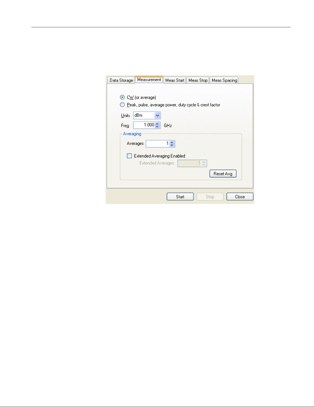
High Speed Logger Application
Measurement
Use the Measure
In order to get accurate measurements you will need to set the frequency. If CW
is selected, only the average or continuous wave power is recorded. If Peak,
pulse… is selected, then all of the indicated parameters are recorded.
ment window to select measurement type, units, and frequency.
RF and Microwave Power Sensors/Met ers 55
Page 70
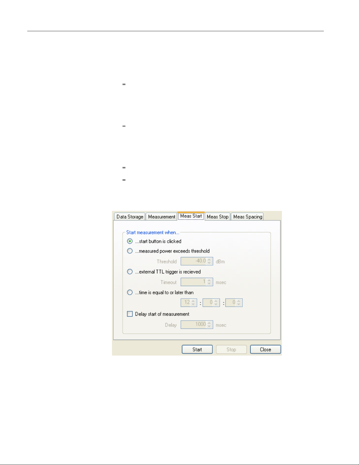
High Speed Logger Application
Meas Start
This window all
processproceedsasfollows:
1. Select the sta
Threshold: Clicking start causes the application to monitor the incoming
measuremen
if peak has been selected). As soon as the appropriate measurement
exceeds the specified threshold, the measurement proceeds. The threshold
is specified in dBm.
External TTL Trigger: Clicking start causes the application to monitor the
external TTL trigger input. When a trigger occurs, measurement will
begin. Only the first measurement requires a trigger. You can set the
trigger timeout. If the timeout occurs before the measurement begins, no
measure
Time of Day: Set the time of day when you want measurements to begin.
Click the start button to begin the measurement process.
2. Execute a delay if desired. The delay begins immediately after the start
criteria has been satisfied and precedes the start of measurements.
ows you to select when to start a measurement. The measurement
rt criteria with one of the following settings:
ts (average power if CW has been selected and peak power
ments will be made.
56 RF and Microwave Power Sensors/Meters
Page 71
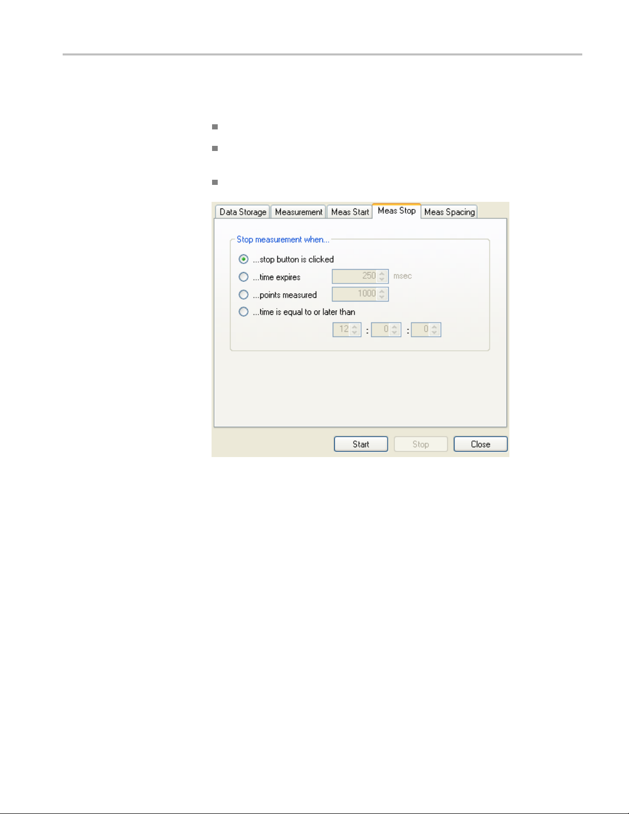
High Speed Logger Application
Meas Stop
Set the criteri
following options:
Stop button: C
Time expires: Specify the time, in milliseconds, when the measurement will
stop.
Points measured: Specify the number of measurements to be taken.
a for stopping a measurement to this window with one of the
lick the stop button to stop the measurement.
RF and Microwave Power Sensors/Met ers 57
Page 72
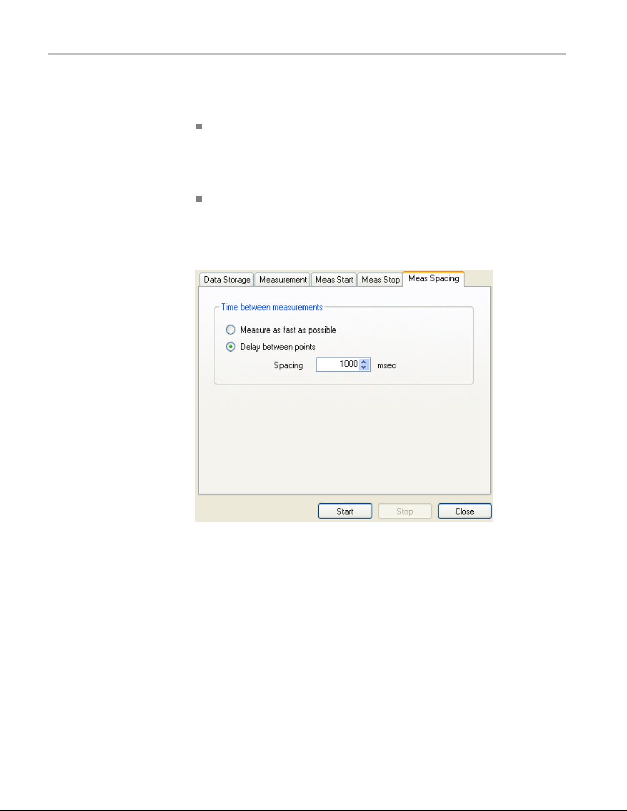
High Speed Logger Application
Meas Spacing
The measuremen
measurements as follows:
Fast as possible: Measures at about 350 μs per point on most computers.
Some computers will be faster, some slower. However, many other factors
may affect this rate. Virtually any loading on the computer may reduce the
rate of measurement. The magnitude of the effect is a function of the power
of the computer and the demands of the competing applications.
Delay between points (in m illiseconds): Set this value to that a delay in the
prescribed number of points causes a stop in meas urement. As stated above,
many factors can negatively impact this rate. Again, these affects tend to be
modest in most cases and pose little concern. In addition, the resolution and
accuracy of the computer clock will have some effect.
t spacing window allow you to define the time between
Make a Simple Measurement
The following information outlines how to make some simple measurements
using this application. These procedures assume that a si
connected and that you have installed the appropriate applications.
1. Start the High Speed Logger Application, selecting Yes to initialize the
instrument.
2. Select the Data Storage tab and click the Browse... button. Select Desktop
(your desktop) and then click OK.
3. Enter TestFile into the File Name text box.
58 RF and Microwave Power Sensors/Meters
ngle instrument is
Page 73

High Speed Logger Application
Troubleshooting
Memory Errors
4. Check the Appen
5. Select Tab Separated Data for the file delimiter.
6. Click the Measurement tab and select CW.
7. Set the units to dBm and the frequency to 1.000 GHz.
8. Click the Meas Start tab and select start button is clicked.
9. Click the Meas Stop tab and select stop button is clicked.
10. Click the M
11. Click the Start button, wait one to two s econds, then click Stop.
12. A Notepad or text file should appear with the data. Depending on the time
between clicking Start and Stop, you may have several thousand lines. If you
used tab
file directly into a Microsoft Excel spreadsheet. You should see the icon for the
file on your desktop and the name of the file should include the date and time.
This application can generate a large amount of data and can consume significant
amounts of memory and disk space. This can cause two problems. This will
probably be because the text file written during measurements is too large for the
application trying to display the file (probably NotePad) if you are running as
t as possible. You can assume that text will be generated at 100 kB/s for CW
fas
measurements, and 250 kB/s for pulse measurements. If your computer runs
out of RAM or disk space, this may also cause a problem. Each measured point
requires (roughly) 54 bytes. If there is not sufficient memory (RAM) and you do
not reduce memory usage, you could run out of RAM.
delimited text, you should be able to copy and paste portions of this
d and View Data boxes if they are not already checked.
eas Spacing tab and select as fast as possible.
To address either problem, reduce the reading rate using the Meas Spacing
settings. For text files,youcanalsoreducethedurationofthetestrunby
adjusting the Meas Start and Meas Stop setting, or deselect the View Data upon
ompletion check box.
C
RF and Microwave Power Sensors/Met ers 59
Page 74

High Speed Logger Application
60 RF and Microwave Power Sensors/Meters
Page 75

Index
A
Address, 48
changing, 17
how to set for instrument, 26
Anti-aliasing, 15, 22
Application
High Speed Logger, 52
how to start, 10
Power Met
Pulse Profiling, 31
Auto Measure
function, 35
panel, 34
window, 35
Averag
Averaging, 21
Averaging & Filters toolbar, 40
e power measurement, 43
er, 19
B
Burst measurements, 23
C
Calibration and zero, 17
CCDF
tistics, 16, 33
sta
CDF
statistics, 16, 33
Center the frequency, 17
Check instrument function, 10
Connect
multiple instruments, 9
to a computer, 6
Connector types, vi
Copy data, 35
Copy trace data, 47
Crest factor measurement, 43
CW (continuous wave), 20
D
Data logger, 25
Defaults
factory, 48
measurement setup, 47
Power Meter, 25
Display Con
Display Options toolbar, 45
Droop measurement, 44
Duty cycle measurement, 43
trol toolbar, 44
E
Error messages, 26
Extended averaging, 21
F
y recall, 48
Factor
Factory setup
recall, 26
Fall time measurement, 43
Filtering
poles, 40
uency, 20, 36
Freq
center the, 17
Frequency response, 2 2
Front panel (virtual)
Power Meter, 19
Functional check, 10
G
ates
G
measurement types, 42
Gates toolbar, 42
H
Help toolbar, 48
Highlight, 32
I
ID, 26, 47
Impedance
input, 24
Input impedance, 24
Installation
computer hardware
requirements, 1
computer requirements, 1
computer sy
requirements, 1
software, 1
USB driver, 6
stem
K
Key features, vi
L
LED, 9
,20
Limits
List of products, vi
M
Main toolbar, 36
Manage named states, 20
Manuals, vii
Markers toolbar, 40
/ Reset, 21
Max
Measured pulse setup, 22
Measurement
functions by model, 13
Measurement range, vi
Measurement Trace window, 32
easurements
M
average (CW) overview, 14
burst, 23
configure for, 17
make CW, 27
make pulse power, 29
make pulse using duty
cycle, 28
pulse overview, 15
pulse profiling overview, 16
resolution, 17
update rate, 23
Menus
moving, 36
RF and Microwave Power Sensors/Met ers 61
Page 76

Index
Minimum loss pa
d, 24
N
Name
how to set for instrument, 26
O
Offset, 22, 37
On/Off ratio measurement, 35
Overshoot measurement, 44
P
Panorami
PDF
Peak power measurement, 43
Pointer Control
Power
Power requirements, 1
Power units, 20
Print toolbar, 46
Products
Pro
Pulse, 20
Pulse power measurement, 43
Pulse Profiling application, 31
Pulse repetition frequency
Pulse repetition time
Pulse setup, 22
Pulse width measurement, 43
c Trace window, 32
statistics, 16, 33
Display Control toolbar, 45
Meter application, 19
list of, vi
gramming examples, 2
toolbar functions, 36
easurement, 43
m
measurement, 43
Q
Quick setup, 25
R
Recall, 20
Recall factory setup
Power Meter, 26
Recall regis
Reference level, 37
Register
recall, 47
store, 47
Reset
Display Co
Reset / Max, 21
Response, 37
Results window, 34
Rise time measurement, 42
ter, 47
ntrol toolbar, 44
S
Safety, v
ecode, 2
Sampl
Save, 20
Sensor ID, 47
Set address, 26, 48
Set Ref, 22
Setup
ck, 25
qui
Single button, 24
Software
installation, 1
Stabilization
thermal, 17
tatistics
S
CDF, CCDF, and PDF, 16, 33
Store register, 47
Store/Recall toolbar, 47
Sweep time, 36
T
Thermal stabilization, 17
Toolbar functi
Pulse Profiling
Trigger
continuous, 39
delay, 39
edge, 39
external TTL, 39
internal auto level, 38
internal manual level, 39
menu, 24
out, 39
single, 24,
single sweep, 39
source, 38
timeout, 39
Triggering & D elay toolbar, 38
ons
application, 36
39
U
undersampling, 15
sampling, 22, 38
Under
Units of power, 20
Update rate, 23
USB
connect multiple
instruments, 1
Bcable, 6
US
USB driver installation, 6
USB requirements, 1
Utility toolbar, 47
W
Windows
moving, 36
Z
Zero and calibration, 17
Zoom
Display Control toolbar, 44
62 RF and Microwave Power Sensors/Meters
 Loading...