Tektronix OM4106D, OM4006D User Manual

Download

OM4106D and OM4006D

ZZZ

Coherent Lightwave Signal Analyzer

User Manual

*P071316002*

071-3160-02

OM4106D and OM4006D

ZZZ

Coherent Lightwave Signal Analyzer

User Manual

www.tektronix.com

071-3160-02

Copyright © Tektronix. All rights reserved. Licensed software products are owned by Tektronix or its subsidiaries or suppliers, and are protected by national copyright laws and international treaty provisions.

Tektronix products are covered by U.S. and foreign patents, issued and pending. Information in this publication supersedes that in all previously published material. Speciﬁcations and price change privileges reserved.

TEKTRONIX and TEK are registered trademarks of Tektronix, Inc.

MATLAB is a registered trademark of The MathWorks, Inc.

LabVIEW is a trademark of National Instruments, Inc.

Intel and Pentium are registered trademarks of the Intel Corporation.

Other prod

uct and company names listed are trademarks and trade names of their respective companies.

Contacting Tektronix

Tektronix, Inc. 14150 SW P.O . Bo x 50 0 Beaverton, OR 97077 USA

For product information, sales, service, and technical support:

In Nor Worl d wide , visi t www.tektronix.com to ﬁnd contacts in your area.

Karl Braun Drive

th America, call 1-800-833-9200.

Warranty

Tektronix warrants that this product will be free from defects in materials and workmanship for a period of one (1) year from the date of shipment. If any such product proves defective during this warranty period, Tektronix, at its option, either will repair the defective product without charge for parts and labor, or will provide a replacement in exchange for the defective product. Parts, modules and replacement products used by Tektronix for warranty work may be n the property of Tektronix.

ew or reconditioned to like new performance. All replaced parts, modules and products become

In order to o the warranty period and make suitable arrangements for the performance of service. Customer shall be responsible for packaging and shipping the defective product to the service center designated by Tektronix, with shipping charges prepaid. Tektronix shall pay for the return of the product to Customer if the shipment is to a location within the country in which the Tektronix service center is located. Customer shall be responsible for paying all shipping charges, duties, taxes, and any other charges for products returned to any other locations.

This warranty shall not apply to any defect, failure or damage caused by improper use or improper or inadequate maintenance and care. Tektronix shall not be obligated to furnish service under this warranty a) to repair damage result b) to repair damage resulting from improper use or connection to incompatible equipment; c) to repair any damage or malfunction caused by the use of non-Tektronix supplies; or d) to service a product that has been modiﬁed or integrated with other products when the effect of such modiﬁcation or integration increases the time or difﬁculty of servicing the product.

THIS WARRANTY IS GIVEN BY TEKTRONIX WITH RESPECT TO THE PRODUCT IN LIEU OF ANY OTHER WARRANTIES, EXPRESS OR IMPLIED. TEKTRONIX AND ITS VENDORS DISCLAIM ANY IMPLIED WARRANTIES OF MERCHANTABILITY OR FITNESS FOR A PARTICULAR PURPOSE.

TRONIX' RESPONSIBILITY TO REPAIR OR REPLACE DEFECTIVE PRODUCTS IS THE SOLE

TEK AND EXCLUSIVE REMEDY PROVIDED TO THE CUSTOMER FOR BREACH OF THIS WARRANTY. TEKTRONIX AND ITS VENDORS WILL NOT BE LIABLE FOR ANY INDIRECT, SPECIAL, INCIDENTAL, OR CONSEQUENTIAL DAMAGES IRRESPECTIVE OF WHETHER TEKTRONIX OR THE VENDOR HAS ADVANCE NOTICE OF THE POSSIBILITY OF SUCH DAMAGES.

[W2 – 15AUG04]

btain service under this warranty, Customer must notify Tektronix of the defect before the expiration of

ing from attempts by personnel other than Tektronix representatives to install, repair or service the product;

Ta ble of Contents

Important safety information ............. ................................ ................................ ........ vi

General safety summary ..................................................................................... vi

Service safety summary ............................ ................................ ......................... viii

Terms in this manual ........... ................................ ................................ .............. ix

Symbols and terms on the product .......................................................................... ix

Compliance information ......................................................................................... xii

EMC compliance ........... ................................ .................................. ............... xii

Safety compliance ........................................................................................... xiii

Environmental considerations............................................................................... xv

Preface ............................................................................................................ xvii

Supported products ......................................................................................... xvii

About this manual .......................................................................................... xvii

Getting started.. ... ... . ... ... ... . . .. . ... ... ... . ... ... ... ... . .. . ... ... . .. . ... ... ... .. .. . ... ... ... .. .. . ... ... ... . ... ... 1

Product description ............. ................................ ................................ ............... 1

Accessories..................................................................................................... 2

Options.......................................................................................................... 2

Initial product inspection. . ... ... ... . ... ... ... . ... ... ... . ... ... ... . ... ... ... . ... ... ... . ... ... ... . ... ... ... . ... . 3

vironmental operating requirements....... ................................ ............................... 4

Power requirements..... ................................ .................................. ..................... 5

PC requirements .................. ................................ .................................. ........... 6

Software installation........................................................................................... 6

Set the instrument IP address................................................................................. 8

Equipment setup .. ................................ .................................. .......................... 13

Operating basics ............... ................................ .................................. .................. 17

OM4000 controls and connectors ............................. ................................ .............. 17

Software overview............................................................................................ 18

The Laser Receiver Control Panel (LRCP) user interface ............................................... 19

The OM4000 user interface (OUI).......................................................................... 23

Conﬁguring the OM4000 user interface (OUI)............................... ................................ .. 57

VISA connections ............ ................................ .................................. .............. 57

Non-VISA oscilloscope connections (Scope Service Utility) .. ... .. .. . ... ... ... . ... ... ... . ... ... ... .. .. 59

Two-oscilloscope conﬁguration ... .................................. ................................ ........ 61

MATLAB ............................... ................................ ................................ ............ 62

Taking measurements ............................................................................................. 63

Setting up your measurement. ... ... . ... ... ... . ... ... . . .. . ... ... . .. . ... ... . .. . ... ... . .. . ... ... . .. . ... ... . .. . . 63

MATLAB Engine ﬁle .. .................................. ................................ .................... 64

Taking measurements ...... .................................. ................................ ................ 65

Multicarrier support (MCS) option . . ... ... ... . ... ... ... . ... ... ... . ... ... ... . ... ... ... .. .. . ... ... ... . ... ... . 66

OM4000D Series Coherent Lightwave Signal Analyzer i

Table of Contents

Detailed conﬁg

References ..................................................................................................... 77

Core processing software guide.... ................................ .................................. ............ 79

Interaction with OUI ......................................................................................... 79

MATLAB variables........................................................................................... 80

MATLAB functions ........................ .................................. ................................ 81

Signal processing steps in CoreProcessing. ................................ ................................ 82

Block processing...................................... .................................. ...................... 87

Alerts management ........................................................................................... 88

Core Processing function reference................................ ................................ .............. 91

AlignTribs ..................................................................................................... 91

ApplyPhase ........................ .................................. ................................ .......... 94

ClockRetime....................................... ................................ ............................ 94

DiffDetection.................................................................................................. 95

EstimateClock................................................................................................. 97

EstimatePhase................................................................................................. 99

EstimateSOP .............. ................................ .................................. ................ 100

MaskCount .................................................................................................. 101

GenPattern................................................................................................... 102

Jones2Stokes .. ................................ ................................ .............................. 103

JonesOrth .................................................................................................... 103

LaserSpectrum .............................................................................................. 104

QDecTh...................................................................................................... 104

zSpectrum.................................................................................................... 106

Appendix A: MATLAB variables used by core processing................................................. 107

Appendix B: Alerts........................ ................................ ................................ ...... 109

Appendix C: Calibration and adjustment (RT oscilloscope).. ... ... ... . .. . ... ... ... .. .. . ... ... ... ... . .. . ... 111

Calibration and adjustment (RT)........ ................................ .................................. 111

Hybrid calibration (RT) .................................................................................... 115

Absolute power calibration ................ ................................ ................................ 119

Laser linewidth factor .................... ................................ ................................ .. 119

Receiver equalization................................... ................................ .................... 119

Appendix D: Automatic receiver deskew..................................................................... 121

Appendix E: Equivalent-Time (ET) oscilloscope operation ... ... . ... ... ... .. .. . ... ... ... .. .. . ... ... ... . .. . 123

Conﬁguring hardware (ET).............. .................................. ................................ 123

Conﬁguring the software (ET) .............. .................................. ............................ 126

OM4000 User Interface (OUI) (ET)................................ ................................ ...... 128

Calibration and adjustment (ET).......... .................................. .............................. 130

Setting up an ET Oscilloscope ... ... ... . .. . ... ... ... ... . .. . ... ... ... .. .. . ... ... ... ... . .. . ... ... ... . .. . ... . 140

Matlab Engine ﬁle (ET).......... ................................ ................................ .......... 141

Taking measurements (ET) ...................... ................................ .......................... 142

uration of experiments ................................ ................................ .......... 77

ii OM4000D Series Coherent Lightwave Signal Analyzer

Table of Contents

OUI overview (E

OUI Controls panel (ET)................................................................................... 142

Analysis Parameters window (ET).......................................... .............................. 143

Appendix F: Conﬁguring two Tektronix 70000 series oscilloscopes . ... ... . ... ... ... . .. . ... ... . .. . ... ... . 145

Oscilloscope settings .. . .. . ... ... . .. . ... ... ... . ... ... ... . ... ... ... .. .. . ... ... ... . ... ... ... . ... ... ... . ... ... . 147

OUI settings for 2-oscilloscope operation . . ... ... ... ... . .. . ... ... . .. . ... ... ... .. .. . ... ... ... . .. . ... ... .. 150

Appendix G:

The LRCP ATE interface ...................... ................................ ............................ 153

The OUI4000 ATE interface............................................................................... 159

ATE functionality in MATLAB .. . ... ... ... . ... ... . . .. . ... ... . ... ... ... . ... ... . . .. . ... ... . ... ... ... . ... ... 167

Building an OM4006 ATE client in VB.NET ... .................................. ...................... 169

Appendix H: Cleaning and maintenance ................................ ................................ ...... 177

Cleanin

Maintenance..................... ................................ ................................ ............ 177

Index

The automated test equipment (ATE) interface ............ .................................. 153

g ......................... ................................ ................................ ............ 177

T)......................................................................................... 142

OM4000D Series Coherent Lightwave Signal Analyzer iii

Table of Contents

List of Figure

Figure 1: Real-time (RT) oscilloscope setup diagram. .. .. . ... ... ... . ... ... ... ... . ... ... ... . .. . ... ... ... . ... .. 13

Figure 2: Eq

Figure 3: Color grade constellation- ﬁne traces ........................ ................................ ........ 45

Figure 4: Color Key constellation ....... ................................ ................................ ........ 45

Figure 5: Multicarrier Setup button (Home ribbon) ........................................................... 66

Figure 6: Multicarrier setup window.................. ................................ .......................... 67

Figure 7: Multicarrier spectrum context menu ................................................................. 69

Figure 8:

Figure 9: Multicarrier spectrum plot details .............................. ................................ ...... 72

Figure 10: Multicarrier constellation plots ... ... ... . ... ... ... .. .. . ... ... ... . ... ... ... ... . ... ... ... . .. . ... ... ... 73

Figure 11: Multicarrier Eye diagrams plot...................................................................... 74

Figure 12: EVM vs. Channel plot ............................... ................................ ................ 74

Figure 13: Q vs. Channel plot.................................................................................... 75

e 14: Meas vs. Channel table .............................................................................. 75

Figur

Figure 15: When adjusting the middle slider, watch the Y-Eye and Y-Const to minimize the signal in the

Y-polarization ............................. ................................ ................................ .. 114

Figure 16: Final channel delay values provide only noise in Y polarization ............... .............. 114

Figure 17: Typical ET oscilloscope setup diagram .. . ... ... ... . .. . ... ... ... . ... ... ... . ... ... ... . . .. . ... ... . 124

Figure 18: ChDelay(2) off by 2 ps causes curvature on constellation and signal on Q-Eye for 28 Gbps

BPS

Figure 19: When adjusting the middle slider, watch the Y-Eye and Y-Const to minimize the signal in the

Y-polarization ............................. ................................ ................................ .. 134

Figure 20: Final channel delay values provide only noise in Y polarization ............... .............. 135

Figure 21: Equivalent-time (ET) oscilloscope setup diagram ... ... . ... ... ... .. .. . ... ... ... . ... ... ... .. .. . . 140

uivalent-time (ET) oscilloscope setup diagram. ... . . .. . ... ... ... . ... ... ... .. .. . ... ... ... . ... ... . 14

Multicarrier spectrum plot ............................................................................ 70

K............................. ................................ .................................. .......... 132

iv OM4000D Series Coherent Lightwave Signal Analyzer

List of Tables

Table 1: Standard and optional accessories...................................................................... 2

Table 2: OM4

Table 3: Software options .... .................................. ................................ ................... 3

Table 4: OM4000 environmental requirements................................................................. 4

Table 5: AC line power requirements ............................................................................ 5

Table 6: List of controller PC (oscilloscope or PC) software . ... ... ... . .. . ... ... ... . ... ... ... . . .. . ... ... ... . .. 7

Table 7: Software install: oscilloscope. . .. . ... ... . .. . ... ... . .. . ... ... ... . ... ... ... . ... ... ... . ... ... ... . ... ... ... . 8

Table 8: O

Table 9: Controls panel elements.. ................................ ................................ .............. 30

Table 10: Record length and block interaction behavior...................................................... 32

Table 11: OUI: Analysis Parameters window...... ................................ ............................ 33

Table 12: Oscilloscope connectivity (VISA vs. Scope Service Utility) .. ... . ... ... . ... ... . . .. . ... . . .. . ... .. 57

Table 13: Multicarrier spectrum menu choices (right-click). ... ... . ... ... ... . ... ... ... . ... ... . . .. . ... ... . .. . . 69

14: Multicarrier spectrum controls . .. . ... ... . .. . ... ... ... . ... ... ... .. .. . ... ... ... . ... ... ... .. .. . ... ... ... 70

Table

Table 15: Alert code descriptions.......................................... ................................ .... 109

000 options .............. ................................ ................................ ........... 2

UI plots (real-time oscilloscopes) ... . ... ... ... .. .. . ... ... ... . ... ... ... . ... ... ... . ... ... ... . ... ... ... 25

Table of Contents

OM4000D Series Coherent Lightwave Signal Analyzer v

Important safety information

Important saf

ety information

This manual c for safe operation and to keep the product in a safe condition.

To safely perform service on this product, additional information is provided at the end of this section. (See page viii, Service safety summary.)

General safety summary

Use the product only as speciﬁed. Review the following safety precautions to avoid injury and prevent damage to this product or any products connected to it. Carefully read all instructions. Retain these instructions for future reference.

Comply with local and national safety codes.

For correct and safe operation of the product, it is essential that you follow generally accepted safety procedures in addition to the safety precautions speciﬁed in this manual.

The product is designed to be used by trained personnel only.

Only qualiﬁed personnel who are aware of the hazards involved should remove the cover for repair, maintenance, or adjustment.

ontains information and warnings that must be followed by the user

To avoid ﬁre or personal

injury

Before use, always check the product with a known source to be sure it is operating correctly.

This product is not intended for detection of hazardous voltages.

Use personal protective equipment to prevent shock and arc blast injury where hazardous live conductors are exposed.

When incorporating this equipment into a system, the safety of that system is the responsibility of the assembler of the system.

Use proper power cord. Use only the power cord speciﬁed for this product and certiﬁed for the country of use.

Do not use the provided power cord for other products.

Ground the product. This product is grounded through the grounding conductor of the power cord. To avoid electric shock, the grounding conductor must be connected to earth ground. Before making connections to the input or output terminals of the product, make sure that the product is properly

Do not disable the power cord grounding connection.

Power disconnect. The power cord disconnects the product from the power source. See instructions for the location. Do not position the equipment so that it

grounded.

vi OM4000D Series Coherent Lightwave Signal Analyzer

Important safety information

is difﬁcult to d all times to allow for quick disconnection if needed.

Observe all terminal ratings. To avoid ﬁre or shock hazard, observe all ratings and markings on the product. Consult the product manual for further ratings information before making connections to the product.

Do not apply a potential to any terminal, including the common terminal, that exceeds the maximum rating of that terminal.

Do not ﬂoat the common terminal above the rated voltage for that terminal.

The measuring terminals on this product are not rated for connection to mains or Category II, III, or IV circuits.

Do not operate without covers. Do not o perate this product with covers or panels removed, or with the case open. Hazardous voltage exposure is possible.

Avoid exposed circuitry. Do not touch exposed connections and components when power is present.

Do not operate with suspected failures. If you suspect tha product, have it inspected by qualiﬁed service personnel.

Disable the product if it is damaged. Do not use the product if it is damaged or operates incorrectly. If in doubt about safety of the product, turn it off and disconnect the power cord. Clearly mark the product to prevent its further operation.

isconnect the power cord; it must remain accessible to the user at

t there is damage to this

Examine the exterior of the product before you use it. Look for cracks or missing pieces.

Use only speciﬁed replacement parts.

Replace batteries properly. Replace batteries only with the speciﬁed type and rating.

Use proper fuse. Use only the fuse type and rating speciﬁed for this product.

Wear eye protection. Wear eye protection if exposure to high-intensity rays or

laser radiation exists.

Do not operate in wet/damp conditions. Be aware that condensation may occur if a unit is moved from a cold to a warm environment.

Do not operate in an explosive atmosphere.

Keep product surfaces clean and dry. Remove the input signals before you clean

the product.

Provide proper v entilation. Refer to the installation instructions in the manual for details on installing the product so it has proper ventilation.

OM4000D Series Coherent Lightwave Signal Analyzer vii

Important safety information

Servi

ce safety summary

Slots and openi otherwise obstructed. Do not push objects into any of the openings.

Provide a safe working environment. Always place the product in a location convenient for v iewing the display and indicators.

Avoid improper or prolonged use of keyboards, pointers, and button pads. Improper or prolonged keyboard or pointer use may result in serious injury.

Be sure your work area meets applicable ergonomic standards. Consult with an ergonomics professional to avoid stress injuries.

Use care when lifting and carrying the product.

Warning- Use correct controls and procedures. Use of controls, adjustments, or proce radiation exposure.

Do not directly view laser output. Under no circumstances should you use any optical instruments to view the laser output directly.

dures other than those listed in this document may result in hazardous

ngs are provided for ventilation and should never be covered or

The Service safety summary section contains additional information required to safely perform service on the product. Only qualiﬁed personnel should perform

ice procedures. Read this Service safety summary and the General safety

serv summary before performing any service procedures.

To avoid electric shock. Do not touch exposed connections.

Do not service alone. Do not perform internal service or adjustments of this

oduct unless another person capable of rendering ﬁrst aid and resuscitation is

pr present.

Disconnect power. To avoid electric shock, switch off the product power and disconnect the power cord from the mains power before removing any covers or panels, or opening the case for servicing.

Use care when servicing with power on. Dangerous voltages or currents may exist in this product. Disconnect power, remove battery (if applicable), and disconnect test leads before removing protective panels, soldering, or replacing components.

Verify safety after repair. Always recheck ground continuity and mains dielectric strength after performing a repair.

viii OM4000D Series Coherent Lightwave Signal Analyzer

Terms in this manual

These terms may appear in this manual:

WAR N ING. Warning statements identify conditions or practices that could result

in injury or loss of life.

CAUTION. Caution statements identify conditions or practices that could result in

damage to this product or other property.

Symbols and terms on the product

Important safety information

These ter

The following symbol(s) may appear on the product:

ms may appear on the product:

DANGER indicates an injury hazard immediately accessible as you read the mark

WARNING indicates an injury hazard not immediately accessible as you read th

CAUTION indicates a hazard to property including the product.

ing.

emarking.

When this symbol is marked on the product, be sure to consult the manual to ﬁnd out the nature of the potential hazards and any actions which have to be taken to avoid them. (This symbol may also be used to refer the user to ratings in the manual.)

OM4000D Series Coherent Lightwave Signal Analyzer ix

Important safety information

Front panel lab

els

Item Description

On inside cover of the instrument

Indicates the location of laser apertures

x OM4000D Series Coherent Lightwave Signal Analyzer

Important safety information

Rear panel labe

Item Description

1 Instrument model and serial number label

Fuse safety information

COMPLIES WITH 21CFR1040.10 EXCEPT

FOR DEVIATIONS PURSUANT TO LASER

NOTICE NO. 50, DATED JUNE 24, 2007

OM4000D Series Coherent Lightwave Signal Analyzer xi

Compliance information

Compliance in

EMC compliance

EC Declaration of Conformity – EMC

formation

This section environmental standards with which the instrument complies.

Meets intent of Directive 2004/108/EC for Electromagnetic Compatibility. Compliance was demonstrated to the following speciﬁcations as listed in the Ofﬁcial Journal of the European Communities:

EN 61326-1 2006. EMC requirements for electrical equipment for measurement, control

CISPR 11:2003. Radiated and conducted emissions, Group 1, Class A

IEC 61000-4-2:2001. Electrostatic discharge immunity

IEC 61000-4-3:2002. RF electromagnetic ﬁeld immunity

IEC 61000-4-4:2004. Electrical fast transient / burst immunity

IEC 61000-4-5:2001. Power line surge immunity

lists the EMC (electromagnetic compliance), safety, and

, and laboratory use.

123

1000-4-6:2003. Conducted RF immunity

IEC 6

IEC 61000-4-11:2004. Voltage dips and interruptions immunity

EN 61000-3-2:2006. AC power line harmonic emissions

EN 61000-3-3:1995. Voltage changes, ﬂuctuations, and ﬂicker

European contact.

ektronix UK, Ltd.

T Western Peninsula Western Road Bracknell, RG12 1RF United Kingdom

This product is intended for use in nonresidential areas only. Use in residential areas may cause electromagnetic interference.

Emissions which exceed the levels required by this standard may occur when this equipment is connected to a test object.

For compliance with the EMC standards listed here, high quality shielded interface cables should be used.

xii OM4000D Series Coherent Lightwave Signal Analyzer

Compliance information

Australia / New Zealand

Declaration o f

Conformity – EMC

Safety complianc

EU declaration of

conformity – low voltage

Complies with t following standard, in accordance with ACMA:

CISPR 11:2003. Radiated and Conducted Emissions, Group 1, Class A, in accordance with EN 61326-1:2006.

Australia / New Zealand contact.

Baker & McKenzie Level 27, AMP Centre 50 Bridge Street Sydney NSW 2000, Australia

he EMC provision of the Radiocommunications Act per the

This section lists the safety standards with which the product complies and other safety compliance information.

Compliance was demonstrated to the following speciﬁcation as listed in the Ofﬁcial Journal of the European Union:

Low Voltage Directive 2006/95/EC.

EN 61010-1. Safety Requirements for Electrical Equipment for Measurement, Control, and Laboratory Use – Part 1: General Requirements.

U.S. nationally recognized

testing laboratory listing

Canadian certiﬁcation

Additional compliances

Equipment type

EN 60825-1. Safety of Laser Products - Part 1: Equipment classiﬁcation and requirements.

UL 61010-1. Safety Requirements for Electrical Equipment for Measurement, Control, and Laboratory Use – Part 1: General Requirements.

CAN/CSA-C22.2 No. 61010-1. Safety Requirements for Electrical Equipment for Measurement, Control, and Laboratory Use – Part 1: General Requirements.

IEC 61010-1. Safety Requirements for Electrical Equipment for Measurement, Control, and Laboratory Use – Part 1: General Requirements.

IEC 60825-1. Safety of Laser Products - Part 1: Equipment classiﬁcation and requirements.

This laser product complies with 21CFR1040.10 except for deviations pursuant to Laser Notice No. 50, dated June 24, 2007.

Test and measuring equipment.

OM4000D Series Coherent Lightwave Signal Analyzer xiii

Compliance information

Safety class

Pollution degree

descriptions

Class 1 – ground

A measure of the contaminants that could occur in the environment around and within a product. Typically the internal environment inside a product is considered to be the same as the external. Products should be used only in the environment for which they are rated.

Pollution degree 1. No pollution or only dry, nonconductive pollution occurs. Products in this category are generally encapsulated, hermetically sealed, or located in clean rooms.

Pollution degree 2. Normally only dry, nonconductive pol Occasionally a temporary conductivity that is caused by condensation must be expected. This location is a typical ofﬁce/home environment. Temporary condensation occurs only when the product is out of service.

Pollution degree 3. Conductive pollution, or dry, nonconductive pollution that becomes conductive due to condensation. These are sheltered locations where neither temperature nor humidity is controlled. The area is protected from direct sunshine, rain, or direct wind.

Pollution degree 4. Pollution that generates persistent conductivity through conductive dust, rain, o r snow. Typical outdoor locations.

ed product.

lution occurs.

Pollution degree rating

IP rating

Measurement and

overvoltage category

descriptions

Mains overvoltage

category rating

Pollution degree 2 (as deﬁned in IEC 61010-1). Rated for indoor, dry location use only.

IP20 (as deﬁned in IEC 60529).

Measurement terminals on this product may be rated for measuring mains voltages from one or more of the following categories (see speciﬁc ratings marked on the product and in the manual).

Category II. Circuits directly connected to the building wiring at utilization points (socket outlets and similar points).

Category III. In the building wiring and distribution system.

Category IV. At the source of the electrical supply to the building.

NOTE. Only mains power supply circuits have an overvoltage category rating.

Only measurement circuits have a measurement category rating. Other circuits within the product do not have either rating.

Overvoltage category II (as deﬁned in IEC 61010-1).

xiv OM4000D Series Coherent Lightwave Signal Analyzer

Environmental considerations

This section provides information about the environmental impact of the product.

Compliance information

Product end-of-life

handling

Restriction of hazardous

tances

subs

Observe the f

Equipment recycling. Production of this equipment required the extraction and use of natural resources. The equipment may contain substances that could be harmful to the environment or human health if improperly handled at the product’s end of life. To avoid release of such substances into the environment and to reduce the an appropriate system that will ensure that most of the materials are reused or recycled appropriately.

Perchlorate materials. This product contains one or more type CR lithium batteries. According to the state of California, CR lithium batteries are

iﬁed as perchlorate materials and require special handling. See

class www.dtsc.ca.gov/hazardouswaste/perchlorate for additional information.

This product is classiﬁed as an industrial monitoring and control instrument,

s not required to comply with the substance restrictions of the recast RoHS

and i Directive 2011/65/EU until July 22, 2017.

ollowing guidelines when recycling an instrument or component:

use of natural resources, we encourage you to recycle this product in

This symbol indicates that this product complies with the applicable European Union re on waste electrical and electronic equipment (WEEE) and batteries. For information about recycling options, check the Support/Service section of the Tekt r on

quirements according to Directives 2002/96/EC and 2006/66/EC

ixWebsite(www.tektronix.com).

OM4000D Series Coherent Lightwave Signal Analyzer xv

Compliance information

xvi OM4000D Series Coherent Lightwave Signal Analyzer

Preface

Supported products

About this manual

This manual d Coherent Lightwave Signal Analyzers.

The information in this manual applies to the following Tektronix products:

OM4006D Co

OM4106D Coherent Lightwave Signal Analyzer

OM1106 Coherent Lightwave Signal Analyzer stand-alone software (OUI) (included with OM4000 Series)

This manual contains the following sections:

Getting started shows you how to install and conﬁgure the OM4000 instrument.

Operating basics provides an overview of the front- and rear-panel controls and connections, and basic operations.

escribes how to install and operate the OM4000 instrument

herent Lightwave Signal Analyzer

Reference provides a MATLAB®function listing.

OM4000D Series Coherent Lightwave Signal Analyzer xvii

Preface

xviii OM4000D Series Coherent Lightwave Signal Analyzer

Getting started

Product description

This section contains the following informationtogetyoustartedusingthe instrument:

Product description

List of instrument accessories and options

Initial product inspection

Operating requirements (environmental, power)

Software, network, and hardware setup

The OM4000 Coherent Lightwave Signal Analyzer is a 1550 nm (C- and L-band) ﬁber-optic test system for visualization and measurement of complex modulated signals, offering a complete solution to test both coherent and direct-detected transmission systems. The OM4000 consists of a polarization- and phase-diverse receiver and analysis software, enabling simultaneous measurement of modulation formats important to advanced ﬁber communications, including polarization-multiplexed (PM-) QPSK.

Key features

The OM4000 User Interface (OUI) software performs all calibration and processing functions to enable real-time burst-mode constellation d iagram display, eye-diagram display, Poincaré sphere, and bit-error detection.

A remote interlock for the laser, located on the rear of the unit, allows for remote locking of laser output.

You can use the OM4000 instrument alo OM2210, as well as supported real-time and equivalent-time oscilloscopes, for a complete optical calibration and testing system.

Coherent lightwave signal analyzer architecture is compatible with both real-time and equivalent-time oscilloscopes

Complete coherent signal analysis syste QPSK, offset QPSK, QAM, differential BPSK/QPSK, and other advanced modulation formats

Displays constellation diagrams, phase eye diagrams, Q-factor, Q-plot, spectral plots, Poincaré sphere, signal vs. time, laser phase characteristics, BER, with additional plots and analyses available through the MATLAB interface

Measures polarization mode dispersion (PMD) of arbitrary order with most polarization multiplexed signals

ng with a Tektronix OM2012 and

m for polarization-multiplexed

OM4000D Series Coherent Lightwave Signal Analyzer 1

Getting started

Accessories

The following table lists the standard and optional accessories provided with the OM4000 instrument.

Table 1: Standard and optional accessories

Tektronix part

Accessory Std. Opt.

OM4106D or OM4006D Coherent Lightwave Signal Analyzer

OM4006D and OM4106D Coherent Lightwave Signal Analyzer U

HRC and LR

HASP USB

Etherne

RF Cabl

Shorti

Power cord

(See p

Reply card

Clea

USB

Chi

tch Cord, Fiber, APC/APC, 8 in. (Opt EXT)

ser Manual (this manual)

CP software USB ﬂashdrive

key

t cable, 7 ft.

e, 2.92 mm, 6 in. (4 cables)

ng cap for BNC interlock connector

age 3, International power cord options.)

ning swab

ﬂashdrive case

na ROHS sheet

●

number

Varies by option

071-3160-xx

650-5643-xx

650-5642-xx

174-6230-xx

174-6229-xx

131-8925-xx

Varies by

optio

Not

rable

orde

Not

rable

orde

016-2067-xx

Not

erable

ord

174-6231-xx

Options

The following table lists some of the options that can be ordered with the OM4000. See the Coherent Lightwave Signal Analyzer OM4000 Series Datasheet (Tektronix part number 52W-27474-x) for a complete listing of options and recommended con ﬁ gurations.

Table 2: OM4000 options

Model Option Description

OM4006D 23 GHz

2 OM4000D Series Coherent Lightwave Signal Analyzer

CC Two C-band lasers

CL One C-band and one L-band laser

LL Two L-band lasers

Table 2: OM4000 options (cont.)

Model Option Description

OM4106D 33 GHz

CC Two C-band lasers

CL One C-band and one L-band laser

LL Two L-band lasers

Getting started

International power cord

options

Tabl e 3: S

Option Description

QAM Adds QAM and other software demodulators

MCS

oftware options

Adds mul

ticarrier superchannel support

NOTE. Option MCS requires that the oscilloscope or PC running the OM

software have an nVidia graphics card installed

All of the available power cord options listed below include a lock mechanism except as otherwise noted.

Opt. A0 – North America power (standard)

Opt. A1 – Universal EURO power

Opt. A2 – United Kingdom power

Opt. A3 – Australia power

. A4–NorthAmericapower(240V)

Opt

Opt. A5 – Switzerland power

Opt. A6 – Japan power

Opt. A10 – China power

Opt. A11 – India power (no locking cable)

Opt. A12 – Brazil power (no locking cable)

Initial product inspection

Do the following when you receive your instrument:

1. Inspect the shipping carton for external damage, whic h may indicate damage to the instrument.

2. Remove the OM4000 instrument from the shipping carton and check that the instrument has not been damaged in transit. Prior to shipment the instrument

OM4000D Series Coherent Lightwave Signal Analyzer 3

Getting started

is thoroughly i

nspected for mechanical defects. The exterior should not have

any scratches or impact marks.

NOTE. Save the shipping carton and packaging materials for instrument

repackaging in case shipment becomes necessary.

3. Verify that the shipping carton contains the basic instrument, the standard accessories and any optional accessories that you ordered. (See Table 1.)

Contact your local Tektronix Field Ofﬁce or representative if there is a problem with your instrument or if your shipment is incomplete.

Environmental operating requirements

Check that the location of your installation has the proper operating environment. (See Table 4.)

CAUTION. Damage to the instrument can occur if this instrument is powered on at

atures outside the speciﬁed ambient temperature range.

temper

Table 4: OM4000 environmental requirements

Parameter Description

Temperature

Relative Humidity

Altitude

Operating +10 °C to +35 °C

Nonoperating

Operating 15% to 80% (No condensation)

Operating To 2,000 m (6,560 feet)

Nonoperating

–20 °C to +70 °C

Maximum operating temperature decreases 1 °C each 300 m above 1.5 km.

To 15,000 m (49,212 feet)

Do not obstruct the fan so that there is an adequate ﬂow of cooling air to the electronics compartment whenever the unit is operating. Leave space for cooling

y providing at least 2 inches (5.1 cm) at rear of instrument for benchtop use.

b Also, provide sufﬁcient rear clearance (approximately 2 inches) so that any cables are not damaged by sharp bends.

4 OM4000D Series Coherent Lightwave Signal Analyzer

Power requirements

Getting started

Table 5: AC line power requirements

Parameter Description

Line voltage r

Line frequency 50/60 Hz

Maximum current 0.4 A

ange

100/115 VAC single phase

230 VAC single phase

WAR N ING. To reduce the risk of ﬁre and shock, ensure that the AC supply voltage

ﬂuctuatio

ns do not exceed 10% of the operating voltage range.

To avoid the possibility of electrical shock, do not connect your OM4000 to a power source if there are any signs of damage to the instrument enclosure.

WAR N ING. Always connect the unit directly to a grounded power outlet.

Operating the OM instrument without connection to a grounded power source could result in serious electrical shock.

CAUTION. Protective features of the OM4000 instrument may be impaired if the

susedinamannernotspeciﬁed by Tektronix.

unit i

Connecting the power cable. Connect the power cable to the instrument ﬁrst, and

connect the power cable to the AC power source. Install or position the

then OM4000 instrument so that you can easily access the rear-panel power switch.

er on the instrument (rear-panel power switch and front-panel standby power

Pow switch). After powering on, make sure that the fan on the rear panel is working. If the fan is not working, turn off the power by disconnecting the power cable from the AC power source, and then contact your local Tektronix Field Ofﬁce or representative.

OM4000D Series Coherent Lightwave Signal Analyzer 5

Getting started

PC requiremen

The equipment and DUT used with the OM4000 determine the controller PC requirements. Following are the requirements to use the OM4000 Series Coherent Lightwave Si

Item Description

Operating system

Processor

RAM

Hard Dri Space

Video Card nVidia dedicated graphics board w/ 512+ MB minimum. graphics memory

Networking

Display

Othe Hardware

LAB

MAT Software

Adobe Reader

gnal Analyzers or OM2210 Coherent Receiver Calibration Source:

U.S.A. Microsoft Windows 7 64-bit

U.S.A. Microsoft Windows XP Service Pack 3 32-bit (.NET 4.0 required)

Intel i7, i5 or equivalent; min clock speed 2 GHz

ntel Pentium 4 or equivalent

4GB

he OUI color grade display feature, the MCS option, and the

using with the O M 4000 Software

2.0 ports

Minimum: I

Minimum:

64-bit releases beneﬁt from as much memory as is available

Minimum: 20 GB

>300 GB recommended for large data sets

NOTE. T

equivalent-time (ET) oscilloscope mode require that the oscilloscope or PC running the OM software have an nVidia graphics card installed

Gigabit Ethernet (1 Gb/s) or Fast Ethernet (100 Mb/s)

20” minimum, ﬂat screen recommended for displaying multiple graph types when

2USB

For Windows 7 (64-bit): MATLAB version 2011b (64-bit)

For Windows XP (32-bit): MATLAB version 2009a (32-bit), .NET version 4

ater.

or l

obe reader required for viewing PDF format ﬁles (release notes,

Ad installation instructions, user manuals).

oftware installation

The OM4000 requires several programs and drivers to be installed on your controlling PC (separate PC or oscilloscope) for proper operation. Install the programs listed in the following table, in the order indicated (starting from the top of table). All programs are on the OM4000 software USB ﬂashdrive unless otherwise noted.

NOTE. Read the installation notes or instructions that are in each application

installation folder before installing each item of software. Only install the software that is appropriate for your OM instrument, PC, and oscilloscope conﬁguration.

6 OM4000D Series Coherent Lightwave Signal Analyzer

Getting started

Install softwa

re on the

controller PC

Table 6: List of controller PC (oscilloscope or PC) software

Program Description Path (from root directory of USB drive)

TekVISA Instrument USB and Ethernet

connectivi

LRCP Laser Receiver Control Panel.

Detects OM instruments on a network, c hardware settings.

MATLAB

OUI OM4000 U

Power meter

HRC Hybrid-Receiver Calibration software.

Required for OUI. Not part of the OM4000 software distribution. Contact The MathWorks, Inc.

The interface for using the OM4000 instrument to take and display

Softwa with the instrument optical power meter. Install in the order listed. Only r software.

Uses SQL to keep track of calibration conﬁ installed automatically if not present on the PC.

ty software.

ontrols laser and other

ser Interface (OUI).

measurements.

re and drivers to communicate

equired for use with the HRC

gurations. SQL software

OUI\ISSetupPrerequisites\TekVISA_v3.3.8\TekVISA\setup.exe

NOTE. Tek V I

series oscilloscopes, or when using the HRC software.

LRCP\LRCPSetup x.x.x.x.msi

to obtain the MATLAB software. See PC requirements to determine the appropri

OUI\Set assumes Matlab 2009a installed)

OUI\SetupOUI_x.x.x.x.exe (Windows 7 64-bit; either Matlab choice)

HRC\IS

HRC\ISSetupPrerequisites\ThorPowerMeterDriver\setup.exe

HRC\Setup Optametra HRC_x.x.x.x.exe

SA is only required when using MSO/DSO70000 or 70000B

ate version of MATLAB for your PC.

upOUI_x.x.x.x 32-bit OS.exe (Windows 7 32-bit or XP 32-bit;

SetupPrerequisites\ThorPowerMeter\setup.exe

Install software on the

oscilloscope

The Scope Service Utility (SSU) is required for MSO/DSO70000C and 70000D series real-time (RT) oscilloscopes, and for the DSA8300 and DSA8200

uivalent-time (ET) sampling oscilloscopes.

Plug the USB ﬂashdrive with the OM4000 software into the oscilloscope. Find

e appropriate Scope Service Utility software installation ﬁle (RT or ET) and

th double-click on the program ﬁle to install it.

NOTE. Read the installation notes or instructions that are in each application

installation folder before installing each item of software. Only install the software that is appropriate for your instrument, PC, and oscilloscope conﬁguration.

OM4000D Series Coherent Lightwave Signal Analyzer 7

Getting started

Table 7: Softwa

Program Description Path

Scope Service Utility

Set the inst

re install: oscilloscope

Enables collecting and analyzing coherent opti on four channels.

There is a separate program for real-time (R (ET) oscilloscopes.

cal signals at 100 Gs/s

T) and equivalent-time

rument IP address

OUI\Tektroni only)

OUI\Tektronix Scope Service For ET Utilityx.x.x.x.exe (install on ET oscilloscop

Use the Laser Receiver Control Panel (LRCP) application to verify and/or set the IP address of OM instruments (OM4106D, OM4006D, OM2210, OM2012) if required f

or your network test setup. All OM instruments must be set to the same network subnet (DHCP-enabled networks do this automatically) to communicate with each other using the LRCP and OM4000 User Interface (OUI) software.

x Scope Service Utilityx.x.x.x.exe (install on RT oscilloscope

e only)

Before using LRCP, you must make sure that IP addresses of the OM series

truments are set correctly to communicate with LRCP on your network. The

ins following sections describe how to set the OM instrument IP addresses for use on DHCP and non-DHCP networks.

8 OM4000D Series Coherent Lightwave Signal Analyzer

Getting started

Set the IP address for

DHCP-enabled networks

The OM instrume default. Therefore you do not need to speciﬁcally set the instrument IP address, as the DHCP server automatically assigns an IP address during instrument power-on (when powering on with the rear-panel power switch).

NOTE. Pushing the front-panel Enable/Standby switch does not automatically

assign a DCHP address; DHCP IP address assignment only occurs when powering on

The following procedure describes how to use LRCP software to verify connecti

Prerequisite: OM instrument, and the controller PC (with LRCP installed), both connect

1. Connect the OM instrument to the DHCP-enabled network.

2. Power on the OM instrument with the rear power switch (set to 1). The

3. On a PC

vity of an OM instrument to a DHCP-enabled network.

ed to the same DHCP-enabled network.

instrument queries the DHCP server to obtain an IP address. Wait until the front p panel Power button to enable the network connection (button light turns On).

LRCP program. (See page 19, The Laser Receiver Control Panel (LRCP) user interface.)

anel Power button light turns off indicating it is ready. Press the front

nts are set with automatic IP assignment (DHCP) enabled by

from the rear-panel Power switch)

connected to the same network as the OM instrument, start the

4. Enter password 1234 when requested.

5. Whe

6. In the Device Setup dialog box, click the Auto Conﬁgure button. LRCP

7. (optional) Use the Friendly Name ﬁeld to create a custom label for each

8. Click OK to close the conﬁgurationdialogboxandreturntotheLRCPmain

n running LRCP for the ﬁrst time after installation, click on the Conﬁguration/Device Setup link on the application screen to open the Device Setup window. Otherwise click the Device Setup button (upper left of application window).

searches the network and lists any O M instruments that it detects. If no devices are detected, work with you IT resource to resolve the connection problem.

instrument. There is no limit to the size of the name you enter.

window. The main LRCP window displays a tab for each instrument detected. Click on a tab to display the laser controls for that instrument. Refer to the LRCP documentation for help on using the software.

OM4000D Series Coherent Lightwave Signal Analyzer 9

Getting started

Set the IP address for a

non-DHCP network

To connect the O default IP address and related settings on the OM instrument to match those o f your non-DHCP network. All devices on this network (OM instruments, PCs and other remotely accessed instruments such as oscilloscopes) need the same subnet values (ﬁrst three number groups of the IP address) to communicate, and a unique instrument identiﬁer (the fourth number group of the IP address) to identify ea

Work with your network administrator to obtain a unique IP address for each device. Yo computer, oscilloscope, and OM instrument. The MAC address is located on the OM instrument rear panel label.

NOTE. Make sure to record the IP addresses used for each OM instrument, or

attach a label with the new IP address to the instrument.

If you a instruments, Tektronix recommends using the OM instrument default IP subnet address of 172.17.200.XXX, where XXX is any number between 0 and 255. Use the operating systems of the oscilloscope and computer to set their IP addresses.

NOTE. If you need to change the default IP address of more than one OM

instrument, you must connect each instrument separately to change the IP address.

re setting up a new isolated network just for controlling OM and associated

M series instrument to a non-DCHP network, you must reset the

ch instrument.

ur network administrator may need the MAC addresses of the

There are two ways to change the IP address of an OM instrument:

Use LRCP on a PC connected to a DHCP-enabled network (easiest)

Use LRCP on a PC set to the same IP address subnet as the OM instrument, to change the OM instrument IP address

Use DHCP network to change instrument IP address. To use a DHCP network to

hange the IP address of an OM series instrument:

1. Dosteps1through6oftheSet network access (DHCP network) procedure.

2. Enter the new IP address for the OM instrument in the AutoConﬁg screen.

3. Click Set IP to set the IP address.

4. Exit the LRCP program.

5. Power off the OM instrument and connect it to the non-DHCP network.

6. Run LRCP and use the Auto Conﬁg button in the Device Setup dialog box to

verify that the instrument is listed.

10 OM4000D Series Coherent Lightwave Signal Analyzer

Getting started

Use direct PC co

connection to change the default IP address of an OM series instrument, you need to:

Install LRPC on the PC

Use the Wind of the current subnet setting of the OM series instrument whose IP address you need to change

Connect the OM instrument directly to the PC, or through a hub or switch (not over a network)

Use LRCP to change the OM instrument IP address

Do the fol of an OM series instrument:

NOTE. The following instructions are for Windows 7.

NOTE. If you need to change the default IP address of more than one OM

instrument using this procedure, you must connect each instrument separately to change the IP address.

nnection to change instrument IP address. To use a direct PC

ows Network tools to set the IP address of the PC to match that

lowing steps to use a direct PC connection to change the IP address

1. On the PC with LRCP installed, click Start > Control Panel.

2. Open the Network and Sharing Center link.

3. Cli

4. Right-click the Local Area Connection entry for the Ethernet connection and

5. Select Internet Protocol Version 4 and click Properties.

6. Enter a new IP address for your PC, using the same ﬁrst three numbers as

7. Click OK to set the new IP address.

8. Click OK to exit the Local Area Connection dialog box.

9. Exit the Control Panel window.

10. Connect the OM instrument to the PC.

11. Power on the OM instrument with the rear power switch (set to 1). Wait until

ck the Manage Network Connections link to list connections for your PC

lect Properties to open the Properties dialog box.

used by the OM instrument. For example, 172.17.200.200. This sets your

C to the same subnet (ﬁrst three number groups) as the default IP address

P setting for the OM series instruments.

front panel Power button light turns off.

OM4000D Series Coherent Lightwave Signal Analyzer 11

Getting started

12. On the PC, start Control Panel (LRCP) user interface.)

13. Enter passwor

14. Select Conﬁguration > Device Setup from the menu to open the Device

Setup windo

15. Click the Auto Conﬁgure button. LRCP lists the OM-series instrument connected t that you entered a correct IP address into the PC and your Ethernet cable is good. If the IP address was entered correctly, you may need to connect the OM instrument to a DHCP network to determine if the IP address you used to set the computer was correct.

16. (optional) Use the Friendly Name ﬁeld to create a custom label for each instrument. There is no limit to the size of the name you enter. Friendly Names are retained and are associated with the MAC address of each instrument.

17. Enter the new IP a ddress for the OM instrument in the AutoConﬁgscreenthat is compatible with your network. For example, 172.17.200.040.

18. Edit the Gateway and Net Mask ﬁelds only if necessary (obtain this information from your network support).

19. Click Set IP.

the LRCP program. (See page 19, The Laser Receiver

d 1234 when requested.

o the PC. If LRCP does not list the connected instrument, verify

NOTE. If you change the instrument to an IP address that is different than

Subnet of the PC, and click Set IP, the OM series instrument is no longer

the detectable or viewable to that PC and LRCP.

20. Click OK to exit the screen and return to the LRCP window.

21. Exit the LRCP program.

22. Unplug the network cable from between the PC and the OM instrument.

onnect the OM instrument to the target network switch/router.

23.C

24. Run the LRCP software on the PC connected to the same network as the

OM instrument.

25. Click Device Setup. Click Auto Conﬁg and verify that the instrument is detected and listed on the display.

12 OM4000D Series Coherent Lightwave Signal Analyzer

Equipment setup

Getting started

Real-time (RT)

oscilloscopes

See the following ﬁgure for how to connect the O M4000 instrument to take measurements with real-time oscilloscopes (Tektronix MSO/DSO70000 series).

Figure 1: Real-time (RT) oscilloscope setup diagram

OM4000D Series Coherent Lightwave Signal Analyzer 13

Getting started

Equivalent-time (ET)

oscilloscopes setup

See the followi

ng ﬁgure for how to connect the OM4000 instrument to take measurements with real-time oscilloscopes (Tektronix DSA8300 or DSA8200 sampling oscilloscopes). Appendix E has more information on using an ET oscilloscope to take measurements. (See page 123, Equivalent-Time (ET) oscilloscope operation.)

Figure 2: Equivalent-time (ET) oscilloscope setup diagram

The most important difference between the real-time (RT) and equivalent-time (ET) oscilloscope measurements is the need for a coherent reference signal for ET oscilloscopes. The TX reference signal is picked off before the modulator, using a PM ﬁber cable, with a total path length equal to the path from the splitting point to the Signal Input on the OM4000 Receiver. Use a SMF ﬁber cable to connect the DUT to the Signal Input connection on the OM4000.

Since the laser phase noise is a real-time quan

tity, it must be sufﬁciently

suppressed so that it can be tracked in the available bandwidth of the ET scope.

As an example, consider a laser with frequency noise given by

f(t) = f

0+fD

sin 2πfnt

If this laser signal is split and then input to the Signal Input and Reference Input of the OM4000, the resulting beat frequency will be

(t) ≈ (2πfDfn∆t) sin 2πfnt

14 OM4000D Series Coherent Lightwave Signal Analyzer

Getting started

Connections

so that while th

, has been reduced by 2πfn∆t where ∆t is the time difference for the two paths.

Some lasers ca

e modulating frequency, f

n have frequency deviations in the 200 MHz range over 1 ms. To

is still the same, the frequency deviation,

minimize the FM bandwidth after detection, reduce the frequency deviation to ~ 1 kHz. This is accomplished with ∆t = 0.8 ns or a path difference of 16 cm or less.

Generally speaking the ET performance will be best with a path difference less than 10 cm when possible. For lower noise lasers, path lengths differences up to 2mcanbetolerated.

Make connections in the following order:

1. Ethernet

connections and other computer connections

2. Power c ord from the OM4000 instrument to the mains AC connector or to the inst

rument rack (if used)

3. Power cord from rack (if used) to mains (keeping m ain front panel switch off)

4. RF connections (the four coaxial cables from OM4000 instrument to the

oscilloscope)

5. Fiber optic PM patch cable connection from Laser 2 to Reference (if needed)

6. Fiber optic Signal input connection

NOTE. Turn off laser optical outputs before attaching cables.

Store all dust covers and coaxial connector caps for future use. Keep dust and coaxial connectors installed on all unused instrument connections.

Power on the equipment and start applications:

1. Controlling PC

2. Oscilloscope

cope Service Utility (SSU) application after the oscilloscope completes its

3.S

power-on cycle

4. OM4000 instrument

When powered on, the OM4000 front-panel power button will light brieﬂyafter main power is applied, indicating it is searching for a DHCP server, and then tun off. Press the power button one time to enable the unit. The steady power button light indicates the instrument is ready for use and that lasers can be activated using the appropriate controller software.

OM4000D Series Coherent Lightwave Signal Analyzer 15

Getting started

The power light or the IP address is changed. Press the power button to re-enable. This feature prevents a remote user from activating the lasers when the local user may not be ready.

NOTE. Ethernet only allows devices on the same subnet to communicate. You

should now have three devices on a localized Ethernet network: computer, oscillosco your corporate network or router or you may choose to leave it isolated.

NOTE. For

controller PC, be sure the controller PC (such as a laptop) has only one Ethernet connection (either wireless or wired) activated.

turns off and the unit is disabled any time AC power is removed

pe, and OM4000 instrument. This little network may be connected to

setup purposes, to ease communication between the LRCP and the

16 OM4000D Series Coherent Lightwave Signal Analyzer

Operating basics

OM4000 contro

Front panel

ls and connectors

1. On/Off standby switch

2. Laser 1 output

3. Optical Input (Signal input)

4. X, Y I/Q

5. Reference Input

6. Laser 2 output (may be internally connected at the factory)

outputs (RF connectors, to connect to the oscilloscope)

OM4000D Series Coherent Lightwave Signal Analyzer 17

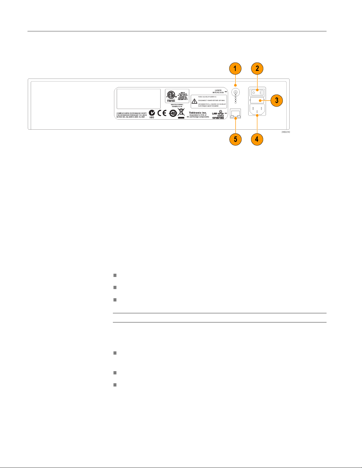
Operating basics

Rear panel

1. BNC connector for optional laser remote interlock

2. Power switch

3. Fuse holder

4. Power cable connector

Software overview

5. 10/100

The OM Interface (OUI) and the Laser Receiver Control Panel (LRCP).

The O

Sets up measurement parameters for the OM4000

Takes input from the OM4000, oscilloscope, and LRCP

Processes data to display a wide assortment of plots

NOTE. The OUI requires the LRCP software to take measurements.

The LRCP:

Detects and provides communication between all detected OM instruments and the OUI.

Sets the OM instrument default IP address

/1000 Ethernet port

4000 instrument uses two primary software programs, the OM4000 User

UI:

Sets OM instrument laser parameters

More information on the LRCP and the OUI are located in the following sections.

18 OM4000D Series Coherent Lightwave Signal Analyzer

Operating basics

The OM4000 also which must be installed on the same PC as the other two applications. The OUI automatically launches the MATLAB application and then interfaces with MATLAB using engine mode. The user does not have to interact with MATLAB for basic operation of the OM4000.

makes use of a third party program, MATLAB by MathWorks,

The Laser Receiver Control Panel (LRCP) user interface

The Laser-Receiver Control Panel application (LRCP) is used to control a variety of Integratable Tunable Laser Assembly (ITLA) lasers. The LRCP interface simpliﬁes the control of the lasers, eliminating the need to use low level ITLA commands. The interface automates locating and conﬁguring all OM devices that are present on the local network. It also provides a Windows Communication Foundation (WCF) service interface, allowing Automated Test Equipment (ATE) to interact directly with the controllers and lasers while LRCP is running.

The main components of the LRCP user interface are:

Menu tabs: Lists available application actions.

Controller tabs: Each tab represents one physical Laser Control device (for example, an OM4000 or an OM2210) on the network. The tab shows the controls for the one or more lasers that are associated with the device.

Status bar: provides important information about the overall state of the communications with the controllers. Each controller has a unique status bar.

Receiver gauge: This gauge displays the total photocurrent output from an instrument. This readout is only functional on devices like the OM4000 instrument that have the appropriate hardware installed.

OM4000D Series Coherent Lightwave Signal Analyzer 19

Operating basics

Device setup and auto

conﬁgure

Connecting to your OM

instruments

Click the Devic dialog box on initial setup of the controllers and anytime network conﬁguration changes and devices are moved to a new IP address. Click the Auto Conﬁgure button to have LRCP search for and list detected OM devices.

An important setting on the Device Setup screen that users will want to adjust is the Friendly Name. Setting this value for each device will aid in the identiﬁcation of the physical location of the controllers as Friendly Names are retained and are tied to the corresponding MAC Address. Make sure to exit the form by clicking the OK butt

The Set IP button is used to modify the addressing as described in the next section. It is not n

Each device must be assigned an IP address in order to communicate with the device. DHCP, will determine the method in which you connect to the devices on your network.

Once co screen. They are listed with the friendly name and IP address to allow for easy identiﬁcation. Lasers are numbered and once the controller is brought online the laser panels will populate with the laser manufacturer and model number.

How you manage IP addresses in your network, namely with or without

nﬁgured and detected, devices are listed as tabs on the main LRCP

e Setup button to open the Device Setup dialog box. Use this

on to save changes.

ecessary to use the Set IP button to change the Friendly Name.

Once the user presses the button that reads Ofﬂine the button will change colors as the control panel attaches to the OM4000 instrument. First, the button will turn yellow and read “Connecting…” indicating that a physical network connection is being established over a socket. Second, the button will turn teal and read

nnected…”. This indicates that a session is established between the device

“Co and Control Panel. Commands will be sent to initialize the communications with the laser and identify their capabilities. Finally, the button will turn bright green when the controller and lasers are ready for action.

NOTE. The button color scheme of bright green meaning running or active,

grey meaning off line or inactive and red indicating a warning or error state is consistent throughout the application.

Once the controller tab is active and the laser panels have populated with the corresponding laser information, you can change the laser settings and/or turn the lasers on. When the controller establishes the connection with the OM4000 hardware, LRCP reads and displays the current hardware state in the laser panel. Any time you exit the application, the current state of the lasers is preserved by the OM4000 hardware, including the emission state.

20 OM4000D Series Coherent Lightwave Signal Analyzer

Operating basics

Setting laser parameters

If the lasers ar laser usage type needs to be set using the dialog on the lower right corner of each laser panel. The OUI uses the setting to determine from which laser frequency information is retrieved. A usage type can only be selected once between all of the tabs but you can have one usage type on one tab and another usage type on a second tab.

NOTE. Only t

other selections are to help identify which laser is which.

Once lase read-only and cavity lock becomes editable. Also the power goes from “off” to the actual power being read from the laser. Readings are taking from the laser once per second.

The receiver gauge (shown at the bottom of the LRCP window) is only active for equipment that have the appropriate hardware present (such as the OM4000 instruments). The receiver gauge, when active, displays the total photocurrent.

NOTE. For all text ﬁeld entries it is necessary to click away from the ﬁeld, or press

the Tab key, for the value entered to be accepted by the application.

e used in conjunction with the OM4000 instrument and OUI, the

he Reference laser selection is important to OUI operation. The

r emission is On, the channel 1 and grid spacing settings become

CAUTION. LRCP does not save the state of any hardware settings. The hardware

keeps the settings until that hardware is turned off. After turning on the hardware again, all settings return to their default state, including emission (which is Off).

Channel: Type a number or use the up/down arrows to choose a channel. The range of channels available will depend on the type of laser, the First Frequenc for a given laser. The channel range is indicated next to the word Channel. The laser channel can also be set by entering a wavelength in the text box to the right of the channel entry. The laser will tune to the nearest grid frequency.

Cavity Lock: The Intel/Emcore ITLA laser that is included in the OM4000 instrument has the ability to toggle its channel lock function. Ordinarily, Cavity Lock should be checked so that the laser is able to tune and lock on to its frequency reference. However, once tuning is complete and the laser needed for locking the laser to its reference. The laser can hold its frequency for days without the beneﬁt of the frequency dither. The OM4000 software will work equally well with the Cavity Lock dither on or off.

y, and the Grid. The ﬁner the Grid, the more channels are available

has stabilized, this box can be unchecked to turn off the frequency dither

OM4000D Series Coherent Lightwave Signal Analyzer 21

Operating basics

Power:Setsthe the desired laser power level. The allowed power range is shown next to the control.

Fine Tune: The Intel/Emcore lasers can be tuned off grid up to 12 GHz. This can be done by typing a number in the text box or by dragging the slider. The sum of the text box and slider values will be sent to the lase r. Once the laser has accepted the new value it will be displayed after the ‘=’ sign.

First Frequency: Not settable. This is the lowest frequency that can be reached by the laser.

Last Frequency: Not settable. This is the highest frequency that can be reached by the laser.

Channel 1:Settablewhenemissionisoff. Thisisthedeﬁnition of Channel 1.

Grid Spacing: Settable (with 100 MHz resolution) when emission is off. 0.1,

0.05 or 0.01THz are typical choices. Use 0.01 THz if tuning to arbitrary (non-ITU-grid) frequencies. Using this grid plus Fine Tune, any frequency in the laser band is accessible.

Laser Electrical Power: This should normally be checked. Unchecking this box turns off electrical power to the laser module. This should only be

d to reset the laser to its power-on state, or to save electrical power if a

neede particular laser is never used.

laser power level. Type or use the up/down arrows to choose

sion:Clicktoturnonorofffrontpanellaseremission.

Emis

Channel setting within the ITLA grid gives the corresponding frequency (in THz)

wavelength (in nm). Power is set within the range allowed by the laser. It is

and best to set the Signal and Reference lasers to within 1 GHz of each other. This is simple if using the internal OM4000 instrument lasers: just type in the same channel number for each.

If using an external transmitter laser, you can type in its wavelength and the controller selects the n earest channel. If this is not close enough, try choosing a ﬁner WDM grid or use the ﬁne tuning feature. If available, ﬁne tuning of the laser is done with the Fine Tune slider bar, and typically works over a range of ±10 GHz from the center frequency of the channel selected.

Certain laser models have a cavity lock feature that increases their frequency accuracy at the expense of dithering the frequency; this feature can be toggled with the Cavity Lock button. Cavity Lock is necessary to tune the laser, but can be unchecked to suppress the dither.

22 OM4000D Series Coherent Lightwave Signal Analyzer

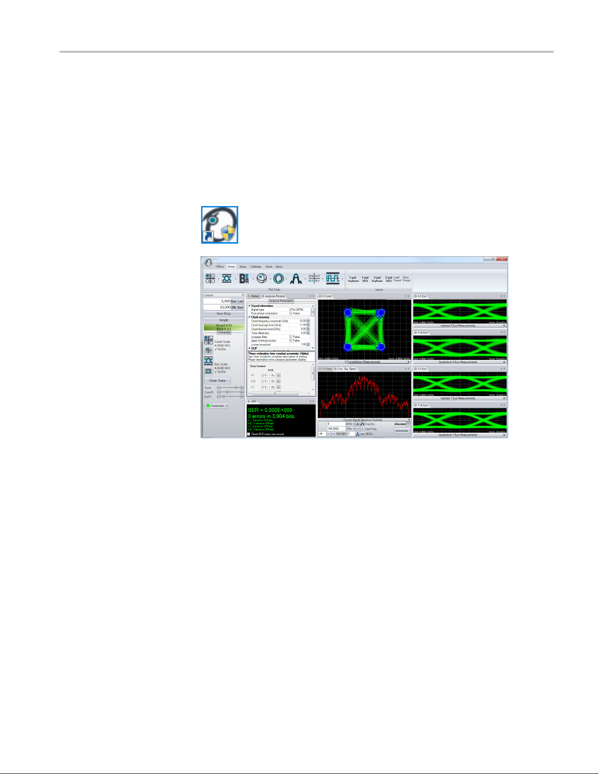
Operating basics

Once the channe laser by clicking on its Laser Emission button; the emission status is indicated both by the orange background of the button and by the corresponding green LED on the OM4000 instrument front panel.

The OM4000 user interface (OUI)

Double-click the OUI desktop icon to open the OM4000 user interface (OUI).

l and power for each laser is set, turn on laser emission for each

The OUI is a ﬂexible panel-based application. You can move panels within the

pplication or drag and position panels from the OUI onto the Windows

OUI a Desktop. Clicking and dragging a panel title tab opens a positioning guide. Hold down the left mouse button to position the window onto the positioning guide, then release to organize the plots.

You can rescale Constellation and Eye plots by clicking on the relevant Plot icons in the Controls panel (located by default on the left side of the OUI application). The scale units are √W/div.

Use the Home tab to set up the plots to display. Click on a Display Format icon in the Plot Tools bar and select a plot type from the menu to display plots relevant to the selected icon. Or select a predeﬁned plot layout from the Layout

ar to populate the OUI with parameter, control, and plot panels for the selected

b measurement.

OM4000D Series Coherent Lightwave Signal Analyzer 23

Operating basics

The OUI is desig There are three types of displays in the OUI: ribbons, ﬂy-out panels, and windows. The Home ribbon, shown below, normally displayed, provides fast access to key tasks. To get more room for readouts or plots, you can hide the ribbon by double clicking in the tab area. Bring it back by double clicking again on one of the tabs.

Click on an icon to see the available menu items from which to select.

Flyout panels are used for information that is needed less often. Click on the

double ar

The graphics windows can be docked or free ﬂoating. To move a graphics window, docking targets will appear as shown below. Moving the pointer to the center of the target w ill cause the window being dragged to be displayed on top of the existing window. Dragging it to one of the four squares surrounding the center of the docking target will split the window so that both the new and old windows are visible. You may also drag the window to another monitor or leave it free ﬂoati

row on a tab

click and hold over the tab then drag. As you drag the window, different

ng in front of the OUI main window.

ned to allow you maximum control of the graphical presentation.

displays or hides the contents of that tab.

24 OM4000D Series Coherent Lightwave Signal Analyzer

Operating basics

OUI plots and

The following t

measurements

Table 8: OUI plots (real-time oscilloscopes)

Plot Description

Constellation Diagram for X or Y signal polarization with numerical readout bottom tabs. Right-click to see graphics options Symbol-center values are shown in blue Symbol errors are sh

3d Eye for X or Y signal polarization. This plot can be scaled and rotated to view on a 2d or 3d monitor. It shows the Constellation Diagram with a time axis modulo two bit periods.

able is an overview of a vailable OUI plots and measurements

own in red Right-click for other color options.

3d Constellation for X or Y signal polarization. This plot can be scaled and rotated to view on a 2d or 3d monitor. It shows the Constellation Diagram with a time axis.

OM4000D Series Coherent Lightwave Signal Analyzer 25

Operating basics

Table 8: OUI plots (real-time oscilloscopes) (cont.)

Plot Description

The coherent eye diagram for X or Y signal polarization shows the In-Phase or Quadrature components vs. time modulo two bit periods. The Q-factor results are provided in a tab below accessed by clicking on the arrows in the lower left corner.

ick on the coherent eye diagram to get options including transition and eye

Right-cl averaging. The transition average shown in red is an average of each logical transition. The calculation is enabled in the Analysis Parameters tab and is used for calculating

on measurements.

transiti

The Pow This is a calculation of the eye diagram typically obtained with a photodiode-input oscilloscope.

Most plots can be viewed in colorgrade by right-clicking on the plot.

Right-click on the X vs T plot to display ﬁeld, averaged-ﬁeld, and symbol quantities. Zoom in o

er Eye shows the computed power per polarization vs time modulo 2 bit periods.

r out or scroll through the record. Error symbols are shown in red.

26 OM4000D Series Coherent Lightwave Signal Analyzer

Table 8: OUI plots (real-time oscilloscopes) (cont.)

Plot Description

BER is shown by physical tributary and in total. Color changes on synch loss.

2d Poincaré shows the position of the data signal polarizations relative to the receiver’s H (1, 2) and V (3, 4).

Operating basics

3d Poincaré shows polarization of each symbol-center value. Click and drag to rotate the sphere.

The Decision-Threshold Q-Factor is an ideal signal quality measurement based on

ured BER values. The horizontal axis corresponds to the vertical axis on the

meas corresponding coherent eye plot. Linear Q is on the left and BER on the right of the plot. Measured values are indicated by squares: blue for 1’s red for 0’s.

OM4000D Series Coherent Lightwave Signal Analyzer 27

Operating basics

Table 8: OUI plots (real-time oscilloscopes) (cont.)

Plot Description

The frequency spectrum of the signal ﬁeld is calculated using an FFT after polarization separation to obtain the spectrum of each signal polarization.

The laser phase noise spectrum is obtained by taking an FFT of the eiθ, where θ is the recov

ered laser phase versus time.

The PMD

Plot provides the results of the PMD calculation

28 OM4000D Series Coherent Lightwave Signal Analyzer

Table 8: OUI plots (real-time oscilloscopes) (cont.)

Plot Description

The Measurements Tab provides a convenient place to ﬁnd almost all of the numerical outputs provided by the OUI with statistics on each value.

Multicarrier measurements. (See page 66, Multicarrier support (MCS) option.)

Operating basics

OM4000D Series Coherent Lightwave Signal Analyzer 29

Operating basics

OUI Controls panel

The Controls pa

nel is typically pinned to the left side for easy access to signal

acquisition and plot scale c ontrols.

Table 9: Controls panel elements

Control Description

Rec Len

Blk Size Block Size. Sets the number of points that are processed at one time.

Record Length. Determines the oscilloscope record length for the next acquisition. The record length in turn determines the horizontal time scale given a ﬁxed sampling rate. Since different oscilloscopes allow different record lengths, the OUI replaces your entry with the closest available larger record length for the connected oscilloscope after you click Single or Run-Stop to start the acquisition.

For record lengths up to 10,000 or even 50,000 points, it makes sense to process everything at once. This will happen if Blk Size is greater than or equal to Rec Len. However, for record sizes above 50,000, there can be a delay of many seconds waiting for processing. In this case, breaking the processing up into blocks gives you more frequent screen updates. Select Blk Size < Rec Len.

The progress bar shows the task completion status. Block Processing is further explained later in the document

Block Processing is most important when the size of the record is so lar g e that it begins to tax the memory limits of the computer. This can begin to happen at 200,000 points but is more like ly a problem at 1,000,000 points and above.

30 OM4000D Series Coherent Lightwave Signal Analyzer

Operating basics

Table 9: Controls panel elements (cont.)

Control Description

For record sizes between 1,000,000 and the oscilloscope memory limit (usually many tens or hundreds of megapoints), it is essential to break processing into blocks to avoid running out of processor memory. In addition, since neither the entire waveform, nor the entire processed variables will ﬁt in computer memory at one time, it is necessary to make some decisions as to what information will be retained as each block is processed. By default, raw data, electric ﬁeld values, and other time series data are not aggregated over all blocks in a record greater than 1,000,000 samples. (See page 53, Managing data sets with record length > 1,000,000.)

Run-Stop The R un button repeatedly takes Single acquisitions until stopped.

Single The Single button takes a single waveform acquisition for processing and

data display.

Scale controls Provides convenient access to change the plot scale setting. Click on the

icons to increment or decrement the setting.

Other controls Other controls will display depending on the selected plots or

measurements.

OM4000D Series Coherent Lightwave Signal Analyzer 31

Operating basics

Analysis Parameters

window

Table 10: Recor

Record length Block size Behavior

<1,000,000 ≥Rec Len All data processed in one block. Aggregated variables

<1,000,000 <Rec Len

>1,000,000 <1,000,000

Any = 1,000,000

d length and block interaction behavior

such as conste plotting.

Data broken up into blocks for processing. Aggregated variables such as constellation and eye diagrams available fo

Data broken and other summary measurements are aggregated block to block. Raw data and time series variables are erased when next b of intermediate blocks of interest for later viewing if this data is needed. Run/Stop mode is disabled.

The maximum allowable entry in the blk size ﬁeld is 1,000,00

llation and eye diagrams a vailable for

r plotting after each block has completed.

up into blocks for processing. Only BER

lock is processed. Need to save workspace

Use the Analysis Parameters window to set parameters relevant to the system and its measurements. Click on a parametertoshowhelponthatiteminthearea at the bottom of the parameter table.

32 OM4000D Series Coherent Lightwave Signal Analyzer

Operating basics

The following c

ontrols are relevant to both equivalent-time and real-time

oscilloscopes except where noted.

Table 11: OUI: Analysis Parameters window

Parameter Description

Signal type Sets the type of signal to be analyzed and the algorithms to be

applied corresponding to that type.

Pure phase modulation

Clock freq (Nominal, Low, H igh)

Time offset Applies an offset in time (horizontal movement on the eye

Lowpass ﬁlter If the edges of a signal are steep or if there is some ringing then

Apply limiting function Some signal distortions may cause the clock component of the

Limiter threshold

Assume Orthogonal Pol

eset SOP Each Block

R (RT oscilloscopes only)

uency

arizations

Sets the clock r ecovery for when there is no amplitude modulation

The nomina bounded by a low (Low) and a high frequency (High), provided the clock signal power is sufﬁcient.

diagram) then the clock recovery process may give a result away from the symbol center. The Time offset adjustment can move it back.

the clo from the symbol center. Switching on the lowpass ﬁlter may cause the eye diagram to become centered. The lowpass ﬁlter is applie seen in the OUI plots.

signal to be weak, so that the eye diagram is shifted in time or the cl in the limiting function may correct these issues. The limiting function is applied in the clock recovery path, and does not affect the s

Thre threshold applies steeper limiting, but may require a longer record length.

Checking this box forces Core Processing to assume that the pol data s ignals have perfectly orthogonal polarization. Making this assumption speeds processing since only one polarization must be the resulting SOPs will be a best effort ﬁt if the signals are not in fact perfectly orthogonal. Unchecking the box forces the code to

earch for the SOP of both data signals.

hecking this causes the SOP to be recalculated for each Block

C of the computation. By adjusting the Block Size (see Blk Size) you can track a changing polarization. When false, the SOP is assumed constant for the entire Record (see R ec Len).

l frequency of the clock recovered by CoreProcessing

to the signal. If a signal has structure, e.g. ringing,

ck recovery process may give an eye diagram displaced

d in the clock recovery path; it does not affect the signals

ock recovery fails (wrong frequency reported). Switching

ignals seen in the OUI.

shold level for clock recovery limiting function. A low

arization multiplexing is done in such a way that the two

found while the other is assumed to orthogonal. In this case,

OM4000D Series Coherent Lightwave Signal Analyzer 33

Operating basics

Table 11: OUI: Analysis Parameters window (cont.)

Parameter Description

2nd Phase Estimate

Homodyne (RT oscilloscopes only)

Phase estimation time constant parameter (Alpha)

Checking this box forces Core Processing to do a second estimate of the laser phase after the data is recovered. This second estimate can catch cycle slips, that is, an error in phase recovery that results in the entire constellation rotating by a m ultiple of 90 degrees. Once the desired data pattern is synchronized with the incoming data stream, these slips can be removed using the known data sequence.

The ﬁrst step in phase estimation is to remove the residual IF frequency that is the difference between the LO and Signal laser frequencies. The function EstimatePhase will fail if it there is no difference frequency. This case occurs when the Signal laser is split to drive both the modulator and the Reference Input of the receiver (ie. only one laser). C hecking the Homodyne box will prevent EstimatePhase from failing by adding an artiﬁcial frequency shift, which is removed by EstimatePhase.

After removing the optical modulation from the measured optical ﬁeld information, what remains is the instantaneous laser phase ﬂuctuations plus additive noise. Filtering the sample values improves the accuracy of the laser phase estimation by averaging the additive noise.

The optimum digital ﬁlter has been shown to be of the form:

-1

1/(1+αz

where α is related to the time constant, τ,oftheﬁlter by the relation

τ =–T/ln(α)

where T is the time between symbols.

So, an α = 0.8 when the baud rate is 10 Gbaud gives a time constant, τ = 450 ps, or a low-pass ﬁlter bandwidth of 350 MHz.

The value of α also gives an indication of how many samples are needed to provide a good implementation of the ﬁlter since the ﬁlter delay is approximately equal to the time constant. Continuing with the above example, approximately 5 samples (~τ/T) are needed for the ﬁlter delay. This of course is not a problem, but an α=0.999 would require 1000 samples and put a practical lower limit on the record length and block size chosen for the acquisition. As a simple rule, the record or block size should be ≥ 10/(1-α).

)

34 OM4000D Series Coherent Lightwave Signal Analyzer

Operating basics

Table 11: OUI: Analysis Parameters window (cont.)

Parameter Description

The selection of the optimum value of Alpha is discussed later in the CoreProcessing guide. (See page 99, EstimatePhase.) This optimum value depends on the laser linewidth and level of additive noise moving from a value near 1 when the additive noise is vastly greater than the phase noise to a value near zero when phase noise is the only consideration (e.g. no ﬁltering needed). In practice, a value of 0.8 is ﬁne for most lasers. If Alpha is too small for a given laser there will be insufﬁcient ﬁltering which is evidenced by an elliptical constellation group with its long axis pointed toward the origin (along the symbol vector). When Alpha is too large then there is excessive ﬁltering for the given laser linewidth. Excessive phase ﬁltering is evidenced by the constellation group stretching out perpendicular to the symbol vector and may also lead to non-ideal rotation of the entire constellation.

As is often the case, when laser frequency wander is greater than the linewidth, very long record lengths will lead to larger variance i n laser phase. This means that an Alpha that worked well with 5000 sample points might not work well with 500,000 points. Longer record lengths will not be a problem if you choose a block size small enough that peak-to-peak frequency wander is on the order of the laser linewidth. For the lasers supplied with the OM4000 instruments, a block size of 50,000 points is a good choice. Refer to Block Processing for more information. (See page 30, OUI Controls panel.)

Signal center freq Sets the approximate center frequency of the signal. If the signal

optical frequency is signiﬁcantly different from the local oscillator frequency, then this control tells Core Processing where it is. If entered incorrectly then frequency aliasing occurs, and the constellation appears to rotate from one symbol to the next.

Balanced Differential Detection (BDD) (RT oscilloscopes only)

Continuous Traces Enables drawing ﬁne trace lines that connect the constellation

Mask Threshold

Symbol Center Width (ET oscilloscopes only)

Sets the differential-detection emulator to emulate balanced instead of single-ended detection.

points. If unchecked, the traces will be suppressed for calculation speed if the calculations are not needed for other plots such as eye diagrams.

Sets the ratio of radius to symbol spacing used for the circular constellation masks.

Sets the fraction of the eye-center that should be considered “symbol center” for the purpose of certain calculations such as which symbols to color blue. The sample closest to symbol center is used to represent that symbol for calculations such as BER and Q-factor.

OM4000D Series Coherent Lightwave Signal Analyzer 35

Operating basics

Table 11: OUI: Analysis Parameters window (cont.)

Parameter Description

Apply Gray coding for QAM

Continuous trace points per symbol

Tributaries contributing to average

Number of symbols in impulse response

Calculate linear average eye

Calculate linear average vs. time

Calculate subsequence average

Subsequence average length

Calculate transition average

Filter type

Filter order

Filter roll-off factor Sets the roll-off factor of the square root raised cosine and raised

Cutoff frequency Sets the cutoff point of the ﬁlter. The cutoff frequency r efers to

Auto-center ﬁlter on signal

If checked then the bit error rate reported with a QAM signal is the BER after applying Gray decoding. The Gray coded BER is typically less than the base BER.

Sets the number of samples per symbol for the clock retiming that is done to create the ﬁne traces in the phase and eye diagrams.

Sets which possible crosstalk contributions are included in the calculation of impulse response. The average waveforms are based on ﬁnding the symbol impulse response and convolving with the data pattern.

Sets the number of values calculated for the impulse response. More values should provide a more accurate average but takes longer to calculate. This control is also used by the adaptive ﬁlter choices (such as Nyquist), which uses the impulse response to calculate the needed ﬁlter.

Controls computation of the average eye. Refresh rate is faster when disabled, but must be enabled for the linear average to be displayed in an eye diagram.

Controls computation of the average signal vs. time. Refresh rate is faster when disabled, but must be enabled for the linear average to be displayed in the X vs. T diagram.

Controls computation of the subsequence averaging. Refresh rate is faster when disabled, but must be enabled for the subsequence a verage to be displayed in the spectrum plots.

Sets the number of symbols in each subsequence.

Controls computation of the transition average. Refresh rate is faster when disabled. However, this must be checked to enable calculations based on transition average such as risetime.

Sets the type of front end ﬁlter, out of Bessel, Butterworth, square root raised cosine, raised cosine, user-deﬁned ﬁlter, matched ﬁlter or Nyquist ﬁlter.

Sets the order of the Bessel and Butterworth ﬁlter types.

cosine ﬁlter types.

the lowpass ﬁlter cutoff point. It is equal to half the width of the ﬁlter as an optical (bandpass) ﬁlter. The cutoff frequency is the 3 d B point of a Bessel, Butterworth or square root raised cosine ﬁlter, and the 6 dB point of a raised cosine ﬁlter.

Sets whether to exactly center the ﬁlter on the signal, or to apply it at the nominal signal center frequency.

36 OM4000D Series Coherent Lightwave Signal Analyzer

Operating basics

Table 11: OUI: Analysis Parameters window (cont.)

Parameter Description

Chromatic D ispersion The value of Dpsnm used by the Compensate CD function in

ps/nm. The sign of Dpsnm should be the same as that of the dispersion compensating ﬁber that it replaces. In other words, Compensate CD i s a dispersion compensator with dispersion of Dpsnm.

Compensate CD Applies a mathematical model to remove Chromatic Dispersion

(CD). T he mathematical model used for the ﬁlter is:

PMD

Use signal description from ofﬂine ﬁle

Use front end ﬁlter from ofﬂine ﬁle

Use calibration from ofﬂine ﬁle

Use carrier deﬁnition table from ofﬂine ﬁle

Data Content

H(ω)=e

where

Polarization Mode Dispersion (PMD) measurement. (See page 52, PMD measurement.)

When selected, applies signal description parameters (signal type, clock frequency, data content) taken from ofﬂine ﬁle. When not selected, applies parameters from Analysis Parameters.

This control has no effect when processing live data.

When selected, applies front end ﬁlter parameters taken from ofﬂine ﬁle. When not selected, applies parameters from Analysis Parameters.

This control has no effect when processing live data.

When selected, applies c alibration data (hybrid, equalization calibration) taken from ofﬂine ﬁle. When not selected, applies calibration data loaded from disk at OUI startup.

This control has no effect when processing live data.

When selected, applies multicarrier carrier deﬁnition table taken from ofﬂine ﬁle. When not selected, applies current carrier deﬁnition table in Multicarrier Setup window.

This control has no effect when processing live data.

For error counting, constellation orientation, and two-stage phase estimation, the data pattern of each tributary must be speciﬁed. Omitting the data speciﬁcation or providing incorrect information about your data pattern will not stop the constellation or eye displays except that there will be no consistent identiﬁcation of each tributary since the identiﬁcation of I and Q and X and Y is arbitrary in the case where the data is not known.

Identify your data patterns for each tributary by choosing a standard PRBS from the drop-down menu, or by assigning the pattern variable directly. Select a user pattern from the drop-down m enu before assigning the variable directly.

iωβ2/2

OM4000D Series Coherent Lightwave Signal Analyzer 37

Operating basics

Front end ﬁlter

Front end ﬁlter group. The ﬁlter is a bandpass ﬁlter in the optical domain, which is equivalent to a lowpass ﬁlter acting on the electrical input signals to the oscilloscope (assuming that the center frequency is zero). The cutoff frequencies speciﬁed are those corresponding to a lowpass ﬁlter. The width of the bandpass (optical domain) ﬁlter is twice the speciﬁed lowpass cutoff frequency.

When Auto-center is checked, the ﬁlter is tuned to the exact center frequency of the signal. Otherwise the ﬁlter is centered at the frequency speciﬁed in the Phase group unde

There are several ﬁlter types available, w hich fall into three ﬁlter categories:

Fixed ﬁlters: Bessel (also known as Bessel-Thomson), Butterworth, square root raised cosine, raised cosine

User-speciﬁed ﬁlter

Adaptive ﬁlters: Matched ﬁlter, Nyquist ﬁlter

The ﬁxed ﬁlter types have their cutoff frequency (either 3 dB point for Bessel, Butterworth and square root raised cosine; or 6 dB point for raised cosine) speciﬁed by the relevant control. The steepness of the ﬁlter is set by the order in the case of Bessel and Butterworth, and by the roll-off factor in the case of the

e root raised cosine and raised cosine ﬁlters.

squar

ing. The signal may be ﬁltered according to the settings of the

r Analysis Parameters.

When the User-speciﬁed ﬁlter is selected as the ﬁlter type, core processing applies

R ﬁlter deﬁned in a variable UserFilter. If the variable does not exist, or if it

an FI is not valid, then core processing continues without applying a ﬁlter, and an Alert is issued in the Alerts w indow to that effect.

UserFilter should have three ﬁelds: .t0, .dt and .Values. The .Values ﬁeld should be a row vector of complex numbers, corresponding to the FIR coefﬁcients. The time grid (speciﬁed by UserFilter.dt) does not have to be the same as the oscilloscope sample time interval, or be synchronous with the symbol rate. Core processing resamples the UserFilter time grid to the input signal time grid before

t is applied. Core processing also tunes the UserFilter in frequency to the center

i frequency speciﬁed in the Phase group of Analysis Parameters, and tunes it to the exact center frequency of the signal if Auto-center is checked. Therefore, the FIR coefﬁcients in UserFilter should be deﬁned so that it is centered at zero frequency.

The matched and Nyquist ﬁlter types are not ﬁxed, but are deﬁnedbasedonthe signal. The matched ﬁ lter type, as its name implies, is the matched ﬁlter having FIR coefﬁcients equal to the time inversion of the signal’s impulse response. The matched ﬁlter is the best possible ﬁlter in terms of the height of an i solated pulse compared to the noise standard deviation. The matched ﬁlter may suffer from intersymbol interference (ISI). In general, a Nyquist ﬁlter is a ﬁlter chosen for a speciﬁc signal to have the property that ther e is no intersymbol interference.

38 OM4000D Series Coherent Lightwave Signal Analyzer

Operating basics

When the Nyquis

t ﬁlter type option is selected a ﬁlter is inserted such that the combination of the signal’s impulse response with the ﬁlter’s impulse response is a Nyquist function, having zero ISI. In principle, there are many possible Nyquist functions. The Nyquist function that has been implemented is a raised cosine function, and the steepness (roll-off factor) of the raised cosine is matched to the steepness of the signal spectrum. With the Nyquist ﬁlter type, the ISI seen in the eye di

agrams should be minimal, but the ﬁlter may not suppress noise

as well as the matched ﬁlter.

The matched and Nyquist ﬁ lters are available in the MATLAB work

space in variables FIR (actual ﬁlter) and FIRCent (centered version). The ﬁlter can be used later as a user-speciﬁed ﬁlter by assigning FIRCent to UserFilter. For example, the Nyquist ﬁlter may be calculated accurately using a long record, and then recalled later to be applied to short records.

Direct assignment of pattern variables.

When the transmitter is sending a PRBS pattern that is not one of the standard patterns provided in the drop-down list, you can assign the PRBS polynomial directly in the MATLAB Engine Command Window in the OUI. The acceptable PRBS polynomials are of the form X in the polynomial X

7+X5

+1, A = 7 and B = 5. This can be assigned to the Real

A+XB

+...+1,whereA>B.Forexample,

tributary of the X-polarization as PattXRe.PRBSGens = [5 7]; shown in the following ﬁgure. Select any standard PRBS in the Analysis Parameters tab. That value will be overridden by the statement in the Matlab Engine Window. Any PRBS polynomial can be speciﬁed in this manner, enabling the use of different sequenceshavingthesamelength. Forexample,[59]and[4679]arebothvalid

9-1

PRBS sequences.

Direct assignment of pattern variables when not using a PRBS. When the transmitter is sending something other than a PRBS, even if it is just a DQPSK pre-code, the analyzer needs to know what data is being sent in order to calculate the BER. In

this case, it is necessary to load your pattern into MATLAB and assign it to the pattern variable. You must also select User Pattern for the data content in the Analysis Parameters tab.

PattXRe.Values = Seq1;

PattXRe.SyncFrameEnd = 100;

PattXlm.Values = Seq2;

OM4000D Series Coherent Lightwave Signal Analyzer 39

Operating basics

PattXlm.SyncF

PattYRe.Values = Seq3;

PattYRe.SyncFrameEnd = 100;

PattYlm.Values = Seq4;

PattYlm.SyncFrameEnd = 100;

rameEnd = 100;

The code assigns the user’s pattern variables Seq1, Seq2, Seq3, and Seq4 to the four tributaries. These variables must be loaded into the separate MATLAB Command Window as shown in the following ﬁgure.

In the case shown, a previously saved .mat ﬁle is loaded and the Seq variable is created using the PattXRe.Values content. The ﬁgure also shows the resulting size of the Seq variable as well as the ﬁrst 10 values. The pattern for each tributary may have any length, but must be a row vector containing logical values.

Synchronizing a long pattern can take a long time. The easiest way to keep

calculations fast when using non-PRBS patterns longer than 2

, and if using record lengths long enough to capture at least as many bits as in the pattern, is to simply use the .SyncFrameEnd ﬁeld as shown above. Otherwise contact customer support for help in optimizing the synchronization.

Example capturing unknown pattern. Another way to load the pattern variable when using a pattern that is not one of the PRBS selections is to use the OUI to capture the pattern and store it in a variable. Do the following:

1. Connect the optical signal with the desired modulation pattern to the OUI.

2. Set up the Analysis Parameters properly with the exception of the data pattern

which is not yet known.

3. Choose Unknown as the data pattern (do not choose “User Pattern” yet).

Optimize the signal to achieve open eye-diagrams and low EVM so that no errors are expected.

40 OM4000D Series Coherent Lightwave Signal Analyzer

Operating basics

4. Set the record l example, you need 32,767 bits to capture a 2

ength long enough to capture the entire data pattern. For

15-1

pattern. Soifthisisat 28 Gbaud and the scope has a sampling rate of 5 0 Gs/s, then you need at least 32,767*50/28 = 58,513 points in the record. Stop acquisition after successfully displaying a good constellation with sufﬁcient record length. All the data you need is now in the MATLAB workspace. It just needs to be put in the prope

r format for use in the pattern variable.

5. In the separate MATLAB Command Window, add the following commands:

For QPSK:

PattXReM = real(zXSymUI.Values) > 0; PattXImM = imag(zXSymUI.Values) > 0;

For dual-pol QPSK add these commands:

PattYReM = real(zYSymUI.Values) > 0; PattYImM = imag(zYSymUI.Values) > 0;

(in addition to above)

6. To get a single full pattern, delete the extra data as follows (in this case for 32,767 bits):

For QPSK:

PattXReM = PattXReM(1: 32767); PattXImM = PattXImM(1: 32767);

For dual-pol QPSK add these commands: (in addition to above)

PattYReM = PattYReM(1: 32767); PattYImM = PattYImM(1: 32767);

7. In the CLSA MATLAB Engine Command Window, add the following lines before the CoreProcessing statement:

For QPSK:

PattXRe.Values = PattXReM; PattXIm.Values = PattXImM;

For dual-pol QPSK add these commands: (in addition to above)

PattYRe.Values = PattYReM; PattYIm.Values = PattYImM;

8. Select User Pattern for any of the tributaries where you assigned a user pattern in the above steps. You should now be able to measure BER using your new patterns.

9. To save the patterns for later use, type the following in the separate MATLAB Command Window:

save(‘mypatterns.mat’,’PattXReM’, ’PattXImM’, ’Pat tYReM’, ’PattYImM’)

OM4000D Series Coherent Lightwave Signal Analyzer 41

Operating basics

Constellation diagrams

Many types of co constellation icon. Once the laser phase and frequency ﬂuctuations are removed, the resulting electric ﬁeldcanbeplottedinthecomplexplane.

When only the values at the symbol centers are plotted, this is called a Constellation Diagram. When continuous traces are also shown in the complex plane, this is often called by the more generic term of IQ Diagram. Since the continuous traces can be turned on or off in the OUI, we refer to both as the Constellation Diagram.

The scatter of the symbol points indicates how close the modulation is to ideal. The symbol points spread out due to additive noise, transmitter eye closure, or ﬁber impa error vector magnitude, or mask violations.

Constellation measurements. Me asurements made on constellation diagrams are the most comprehensive in the OUI. Numerical measurements are available on the ﬂyout panel associated with each graphic window. The measurements available for con

irments. The scatter can be measured by symbol standard deviation,

stellations are described in the following text.

nstellation diagrams can be chosen by clicking on the

Elongation: The mean inter-symbol spacing of the quadrature signals divided by the mean inter-symbol spacing of the in-phase signals. “Tall” constellations have Elongation > 1.

Real Bias: The real part of the mean value of all symbols divided by the magnitude; expressed as a percent. A positive value means the constellation is shifted right.

42 OM4000D Series Coherent Lightwave Signal Analyzer

Operating basics

Imag Bias: The i by the magnitude; expressed as a percent. A positive value means the constellation is shifted up.

Magnitude: The mean value of the magnitude of all symbols with units given on the plot.

Phase Angle: The phase angle between the two tributaries.

StdDev by Qu the mean symbol in units given on the plot. This is displayed for BPSK and QPSK.

maginary part of the mean value of all symbols divided

adrant: The standard deviation of symbol point distance from

(%): The rms distance of each symbol point from the ideal symbol point

EVM divided by the magnitude of the ideal symbol expressed as a percent.

Tab: The separate EVM tab shown in the right ﬁgure provides the

EVM EVM% by constellation group. The numbers are arranged to correspond to the symbol arrangement.

Mask Tab: The separate Mask tab shown in the right ﬁgure provides the number of Mask violations by constellation group. The numbers are arranged to correspond to the symbol arrangement.

OM4000D Series Coherent Lightwave Signal Analyzer 43

Operating basics

The Q calculati transitions. For example, in 32-QAM. 32-QAM is a subset of 64-QAM, where the outer constellation points are never used. It is not possible to calculate a Q factor for those outer slices, hence the alert. The subconstellation identiﬁcation feature notices the unused constellation points, and removes them from the relevant constellation parameters (zXSym.Mean, zXSym.ConstPtMean, etc.), but that happens in E does not know that the outer constellation points never occur, and so it generates the appropriate alert, but it does continue processing. (See page 104, QDecTh.)

Offset modulation formats. Both polarization and quadrature offset formats are available. To properly display polarization offset formats, select Home >

Constell

in the following ﬁgure.

hat the Y polarization is a half-symbol offset from the X polarization;

Note t the standard “Y const” display will be empty, and the offset (or intermediate) constellation display is selectable from the constellation pull-down menu as shown in the upper left-hand corner.

on can cause alerts if it can’t calculate a Q factor for the outer

ngineCommandBlock, after the Q calculation has occurred. QDecTh

ation button > Y Intermediate Constellation as the display, as shown

Color features. A new feature (dependent on your PC video adapter capabilities),

inning with Version 1.2.0, is the ability to Right-Click on any constellation

beg window and get a list options including Color Grade, Display Traces in Color Grade, and Color Key Constellation Points.

44 OM4000D Series Coherent Lightwave Signal Analyzer

Figure 3: Color grade constellation- ﬁne traces

Operating basics

The Color Grade option provides an inﬁnite persistence plot where the frequency of occurrence of a point on the plot is indicated by its color. This mode helps reveal patterns not readily apparent in monochrome. Persistence can be cleared or

m the Right-Click menu as well.

set fro

Figure 4: Color Key constellation

Color Key Constellation Points is a special feature that works when not in Color Grade mode. The value of the previous symbol determines the symbol color. This helps reveal pattern dependence.

OM4000D Series Coherent Lightwave Signal Analyzer 45

Operating basics

Eye diagrams

The Color Key co

lors:

If the prior symbol was in Quadrant 1 (upper right) then the current symbol is colored Yel

low

If the prior symbol was in Quadrant 2 (upper left) then the current symbol is colored Mag

enta

If the prior symbol was in Quadrant 3 (lower left) then the current symbol is colored l

ight blue (Cyan)

If the prior symbol was in Quadrant 4 (lower right) then the current symbol is colored

solid Blue

Eye diagram plots can be selected for appropriate modulation formats by clicking on the eye-diagram icon and selecting an eye format. Supported eye formats include

ﬁeld Eye (which is simply the real part of the phase trace in the complex plane), Power Eye (which simulates the Eye displayed with a conventional oscilloscope optical input), and Diff-Eye (which simulates the Eye generated by using a 1-bit delay-line interferometer). As with the Constellation Plot you can right-click to choose color options as well.

The ﬁeld Eye diagram provides the following measurements:

Q (dB): Computed from 20*Log10 of the linear decision threshold Q-factor of the eye

Eye Height: The distance from the mean one level to the mean zero level (units of plot)

Rail0 Std Dev: The standard deviation of the 0-Level as determined from the decision threshold Q-factor measurement

Rail1 Std Dev: The standard deviation of the 1-Level as determined from the decision threshold Q-factor measurement

In the case of multi-level signals, the above measurements will be listed in the order of the corresponding eye openings in the plot. The top row values correspond to the top-most eye opening.

The above functions involving Q factor use the decision threshold method

described in the paper by Bergano

. When the number of bit errors in the measurement interval is small, as is often the case, the Q-factor derived from the bit error rate may not be an accurate measure of the signal quality. However, the decision threshold Q-factor is accurate because it is based on all the signal values, not just those that cross a deﬁned boundary.

N.S. Bergano, F.W. Kerfoot, C.R. Davidson, “Margin measurements in optical ampliﬁer systems,” IEEE Phot. Tech. Lett., 5, no. 3, pp. 304-306 (1993).

46 OM4000D Series Coherent Lightwave Signal Analyzer

Operating basics

Signal vs. Time

Several plots o Signal vs. Time after clicking the waveform icon under the Home tab of the main ribbon. Sig vs T is different from other plots in that it allows many different variables to be displayed, and the user chooses which variables. The plot displays only the inphase X polarization ﬁeld component when created. Right clicking the plot opens a context menu with X and Y polarization menus, and hovering the mouse shows

f ﬁeld components as a function of time are available by selecting

a list of available selections.

The ﬁeld options are the as-measured electric ﬁeld components, plotted as green lines. The symbol options draw blue dots at the symbol center times. The linear average is discussed in a later section, and is plotted as yellow lines. (See page 48, Waveform averaging.)

Clicking the mouse scroll wheel zooms the Sig vs T plot in time, and the scroll bar along the bottom shows how much of the record is being displayed. Slide the horizontal scroll bar to offset the plot in time. t0 is the plot center relative to the trigger time. Errored symbols are shown in red.

OM4000D Series Coherent Lightwave Signal Analyzer 47

Operating basics

Waveform averaging

Two types of ave available. These show a cleaner version of the signal, having a reduced level of additive noise. The transition average is available by checking Averaging: Show Transition Average under Analysis Parameters and selecting Show Transition Average from the right click menu of the eye diagram where the average is to be displayed. The red trace shows the average of the different transitions between levels: 0-0

The transition parameters listed in the X-Trans, Y-Trans and Pow-Trans sections

Measurements table are derived from the transition average curves.

of the Transition average is available for the ﬁeld component eye diagrams, and if the modulation format is an OOK type, for the power eye d iagram.

raged display of the eye diagram and signal vs. time are

, 1-1, 0-1 and 1-0.

The linear average is made visible by checking Averaging: Show Linear Average Eye or Show Linear Average vs. Time. The average is displayed as yellow traces in any ﬁeld eye diagram or Signal vs. Time plot where the linear average is selected from the right click menu.

48 OM4000D Series Coherent Lightwave Signal Analyzer

Operating basics

The linear average is obtained using a two-step process:

The impulse response associated with the signal is calculated by a deconvolution process

That impulse response is applied to the known data content of the signal to produce a linear average.

The linear average assumes that the signal has a linear dependence on the data bits. If there is nonlinearity, for example if the crossing point is higher than 50%, then the linear average is a poor ﬁt to the actual waveform.

The linear average can provide useful information about the nature of the signal. The length of the impulse response is set by Averaging: Number of Symbols in

se Response. Typically the average eye diagram appears noisier as the

Impul impulse response length is increased, because the number of traces in the eye diagram increases. However if the true impulse response of the signal has a long duration, for example if there is a reﬂection from a length of RF cable inside the transmitter, then the linear average eye diagram will clean up once the impulse response length is made long enough to capture that reﬂection event.

There a re several options of which tributaries to take into account when calculating the impulse response, selected from Averaging: Tributaries contributing to

erage. The basic option is Same trib only, which typically gives the cleanest

av result. It is possible to include other tributaries and exclude the same tributary, for example Other SOP tribs. This setting computes the impulse response only by taking into account the signal on the other state of polarization. For an ideal signal the linear average computed this way should be a ﬂat line. If there is structure on the linear average waveform then that suggests there is a crosstalk mechanism between the states of polarization.

The impulse response variables are available in the MATLAB workspace in variable Imp, which has ﬁelds .XRe, .XIm, .YRe and .YIm.

OM4000D Series Coherent Lightwave Signal Analyzer 49

Operating basics

Current Signal Spectrum

plot

The Current Sig button on the Home tab. Right-click on the plot to select what to display. The OUI displays the input signal spectrum by default.

nal Spectrum plot is accessed by clicking on the spectrum icon

Measurements Statistics

table

The Measurement Statistics table is displayed by the Tabular-Data menu (click on the Tabular Data icon). The Measurements Statistics table contains essentially every measurement made by the OUI with statistics. In cases such as EVM or Q-factor for QAM, where there may be too many numbers to list in the table, the table shows an average for each tributary. The detailed values by constellation group are found on the constellation, eye, or Q plots, and are also available in the MATLAB workspace.

The table shows the following measurements:

X-Eye (Y-Eye): These are the measurements related to the decision-based Q-factor method. Sweeping the decision threshold value while computing the resulting BER, provides a measure of the Eye Height, and standard deviations of each ra il.

X-Const (Y-Const): These measurements are made on the constellation groups calculated for the constellation diagram display.

X-Trans ( Y-Tra n s) : The transition parameter measurement is based on the Transition Average. (See page 48, Waveform averaging.) The values listed are measured on the averaged transition.

Pow-Trans: Is the transition parameters for power signal. These values are only calculated for the power signalingtypessuchasOOKandODB.

XY Measurements: Sig Freq Offset is the calculated difference by between Signal and Reference Lasers. Signal Baud Rate is the recovered Clock

50 OM4000D Series Coherent Lightwave Signal Analyzer

Operating basics

2D Poincaré sphere

Frequency. PER

is the polarization extinction ratio of the transmitter calculated when Assume Orthogonal SOPs is no checked. PDL is the relative size of the X and Y constellations (PDL of a PM modulator).

PMD:(Seepage52,PMD measurement.)

The Core Processing software locks on to each polarization signal. Depending on how the

signals were multiplexed, the polarizations of the two signals may or may not be orthogonal. The polarization states of the two signals are displayed on a circular plot representing one face of the Poincaré sphere. States on the back side are indicated by coloring the marker blue.

The degree of orthogonality can be visualized by inverting the rear face so that orthogonal signals always appear in the same location with different color. Thus Blue means back side (negative value for that component of the Stokes vector), X means X-tributary, O means Y-tributary, and the Stokes vector is plotted so that

t, down, blue are all negative on the sphere.

lef

InvertedRearFace: checking this box inverts the rear face of the Poincaré sphere

splay so that two orthogonal polarizations will always be on top of each other.

CoreProcessing reports pXSt and pYst organized Q, U, V in the terminology

own below. These values are plotted as X,Y pairs (Q,U) with V determining the

sh color (blue negative). The plot is from the perspective of the “North Pole.”

=|E

|2+|Ey|

Q= |Ex|2-|Ey|

U=2 Re(ExEy*)

V=2 Im(E

xEy

OM4000D Series Coherent Lightwave Signal Analyzer 51

Operating basics

Bit-Error-Rate reporting

PMD meas

urement

Bit error rates

are determined by examination of the data payload. You may choose BER or Differential BER. Differential BER compares the output of a simulated delay-line interferometer to a differential form of the data pattern speciﬁed in the Analysis Parameters. If you choose to pre-code your data signal prior to the modulator as in a typical differential transmitter, you will need to enter the patterns seen at the I and Q modulators into the respective pattern variables, (for exampl

e, PattXRe.Values and PattXIm.Values). If no pre-coding is used, then you may use the drop-down menus to specify standard PRBS codes. (See page 38, Front end ﬁltering.)

For multilevel signal types such as QAM, the Gray code BER or the direct BER may be reported. The check box BER: Apply gray coding for QAM under Analysis Parameters selects which BER type is reported. More information is given in a detailed application note on automated BER measurements at the end of this manual.

Polarization mode dispersion (PMD) is an effect associated with propagation through long distances of optical ﬁber that degrades the signal through inter-symbol interference. It is described by several coefﬁcients. Often the ﬁrst

and second order coefﬁcients are all that is needed. The OUI can estimate the

order amount of PMD that a signal has experienced from the structure of the waveform. The met hod used is described in the research paper by Taylor

.ThePMD measurement works with dual polarization signals. Two kinds of measurement are possible, reference based and non-reference based, according to the check box in PMD: Use PMD Reference under Analysis Parameters. If the non-reference based

surement is chosen then the OUI estimates the PMD directly from the signal.

mea The ﬁrst and second order PMD values are reported in the Measurements window.

e reference based measurement is sometimes more accurate than the

Th non-reference based measurement. If the signal itself has an offset in time between the X and Y polarizations then with the non-reference mea surement that offset is effectively added to the reported PMD values. With the reference based measurement, that offset between polarizations is taken into account, by ﬁrst acquiring a measurement (the reference) direct from the transmitter.

It is necessary to tell the OUI when the reference is being acquired, and that is done by checking the PMD: Acquire PMD Reference check box. When the reference measurement is complete this check box must be unchecked. The reference-based measurement uses a linear impulse response, and the settings under Averaging (See page 48, Waveform averaging.), also apply to the reference-based PMD measurement. The PMD: Measure PMD check box must be checked for the PMD values to be reported in the Measurements window.

M.G. Taylor & R.M. Sova, “Accurate PMD Measurement by Observation of Data-Bearing Signals,” IEEE Photonics Conf. 2012, paper ThS4, Burlingame CA, 2012.

52 OM4000D Series Coherent Lightwave Signal Analyzer

Operating basics

Recording and playback

Alerts

Managing data sets with

record length > 1,000,000

You can record t the Record button in the Ofﬂine ribbon. These are recorded to C:\Users\<user>\Documents\TekApplications\OUI\MAT Files.

You can play back the workspace from a sequence of .mat ﬁles by ﬁrst using theLoadbuttonintheOfﬂine Commands section of the Home ribbon. Load a sequence by marking the ﬁles you want to load using the Ctrl key and marking the ﬁlenames with the mouse. You can also load a contiguous series using the Shift key and marking the ﬁrst and last ﬁlenames in the series with the mouse.

UsetheRunbuttonintheOfﬂine Commands section of the Home ribbon to cycle through the .mat ﬁles you recorded. OUI uses the ﬁlter settings stored in the .mat ﬁ

You can override the .mat ﬁle settings with certain Analysis Parameter settings by using th This makes it possible to reprocess the saved data using different ﬁlters or other settings, rather than those settings stored in the .mat ﬁle. (See page 37.)

See th

It is important to break up records larger than 1,000,000 points into blocks that can ﬁt into the computer memory. This is done by setting the Blk Size to something betw of progress updates and overall processing time. When operating in this mode, only the number of errors and other numerical measurements are maintained from block to block. Time series information such as electric ﬁeld values and raw data are discarded to conserve memory. This means that if you do nothing else, the large acquisition will end with only the ﬁeld and symbol values for the last block

ailable along with the BER, EVM, and measurements which are collected over

av the entire record. It is important in the large-acquisition case to learn how to save intermediate data sets if the time-series data is needed.

les.

eOfﬂine controls near the bottom of the Analysis Parameters window.

e Appendix for alert messages information. (See page 109, Alerts.)

een 10,000 and 200,000. Typically 50,000 is a good balance between speed

he workspace as a sequence of .mat ﬁles using

Saving intermediate data sets: examples. The simplest way to save intermediate data is to record every record. (See page 52, PMD measurement.) However, this may generate a very large set of ﬁles that will then need to be analyzed later. If you only want to save the workspace on a particular event, you can use the save command after the CoreProcessing call.

Once you have saved the data sets, you can view them later by using the Load command described earlier. You can load them one at a time or as a group to see a replay. Just be sure the correct analysis parameters are being used. If you save the entire workspace by omitting the variable names in the save statement, then you can also open the .mat ﬁles later in MATLAB and use MATLAB plots to examine the variables.

OM4000D Series Coherent Lightwave Signal Analyzer 53

Operating basics

There are two pa

rts to setting this up. First you need a unique ﬁle name that can be created automatically, second you need to design an if-statement to trigger on the proper event.

Examples of save statements for unique ﬁle names. The following command saves data to ﬁles with the name testn.mat, where the n is replaced with whichever block is being processed at the time.

This is simple but has the drawback that the ﬁles will be overwritten by future acquisitions that happen to save on the same test name and block numbers.

save([‘test’,num2str(BlockNum),’.mat’],’Vblock’)

The following example saves the entire workspace to time-stamped ﬁlenames of the form Test11_4_2009_12_24_53.mat., with the ﬁrst string (Test) followed by parts of the Clk string with the month (2), day (3), year (1), hour (4), minute (5), and second (6) the save was executed.

Clk = clock;

save(['Test',num2str(Clk(2)),'_',num2str(Clk(3)),'_', num2str(Clk(1)),'_', ...

num2str(Clk(4)),'_',num2str(Clk(5)),'_', num2str(round(Clk(6))),'.mat'])

Examples of if-statements and alerts to trigger a save. The following example (when placed after the CoreProcessing call in the MATLAB window) saves the Vblock variables every time there is a bit error on the XRe tributary. The Vblock variables are really all that are necessary for later analysis, but saving the whole workspace can help be sure that the original processing information, such as patterns and signal type, are not lost.

In the following example, using BER.NumErrs, instead of NumErrs.XRe, has the effect of trigging on any error in any tributary, rather than just XRe.

if Errs.XRe.NumErrs>0

Clk = clock;

save(['HybridCal',num2str(Clk(2)),'_',num2str(Clk(3)),'_', num2str(Clk(1)),'_', ...

54 OM4000D Series Coherent Lightwave Signal Analyzer

Operating basics

UsingtheOUIwithother

receivers

num2str(Clk(4 '.mat'], Vblock)

end

)),'_',num2str(Clk(5)),'_',num2str(round(Clk(6))),

The following example triggers on an alert, using the Alert variable existence or thetypeofalertasatrigger

if(isfield(Alerts,'Active'))

Clk = clock;

save(['HybridCal',num2str(Clk(2)),'_',num2str(Clk(3)), '_',num2str(Clk(1)),'_', ...

num2str(Clk(4)),'_',num2str(Clk(5)),'_',num2str(round(Clk(6))), '.mat'], Vblock)

end

The OUI software may be used to process data taken from any receiver that has the following properties:

The signal is linear. This means that AGC ampliﬁers (if used) must be put in ﬁxed gain mode.

Stable over the measurement time. The OUI software uses calibration routines to correct for receiver optical properties such as gain, skew, and phase angle error. If the receiver properties change signiﬁcantly between the time of calibration and the time of using the calibration data, then you will not get optimal results. It is still possible to assume ideal receiver properties.

To use a receiver other than the OM-Series, follow the same set

up and calibration

procedure as for the OM4000 instrument with the following exceptions:

1. Disable the automatic hybrid calibration. This can be done by placing the following statement in the Engine Command Window in the OUI prior to the CoreProcessing statemen t:

pHyb=[1i00;001i];

2. Disable the factory frequency response equalization for the OM4000. This can be done by placing the following statement in the Engine Command Window in the OUI prior to the CoreProcessing statement: EqFilt(1).dt = 1; This can go before or after the pHyb statement.

3. Follow the other calibration procedures(Seepage111,Calibration and adjustment (RT oscilloscope).). In the case of Hybrid Calibration (See

OM4000D Series Coherent Lightwave Signal Analyzer 55

Operating basics

page 115, Hybrid ca

libration (RT).), put the following statement in the Engine

Command Window in the OUI before the DispCalEllipses statement:

CorrectPhase

= true;

The resulting pHyb statement replaces the one in step 1. Hybrid Calibration is optional

if the receiver gain and phase accuracy is good enough to be

approximated by the ideal hybrid model in step 1.

After conne

cting and calibrating the receiver, it is ready for use with the OUI

software.

To emulate

the behavior of a deployed rec eiver:

The OM4000 product is an analyzer for understanding the physical performa

nce of transmitters and optical communication links. It uses ﬁxed calibration parameters to remove uncertainties. Deployed receivers will run algorithms to correct in real time for skew, gain, and phase errors of the receiver, being concerned more about data integrity rather than physical measurement accuracy. To emulate this function of the receiver, it is important to follow the calibration steps 1- 3, and to repeat the calibration when the

ver properties change.

recei

A deployed receiver will also run an adaptive algorithm that optimizes the

ency response of the receiver. To emulate this function, use the adaptive

frequ ﬁlter algorithm provided (you may have to ask for this as it is distributed separately.)

56 OM4000D Series Coherent Lightwave Signal Analyzer

Conﬁguring the OM4000 user interface (OUI)

Start the OUI with the icon on your desktop or in the programs menu.

NOTE. Be sure that MATLAB is available and properly licensed, since the

OUI attempt if MATLAB is not available.

s to launch a matlab command window, and will appear to stall

Connectin

g to the oscilloscope upon OUI startup is done with the Connect button in the Scope Setup section of the Setup ribbon. Notice that there are two choices for making an oscilloscope connection: VISA and non-VISA. VISA is only necessary when working with older real-time oscilloscopes. (See Table 12.)

Table 12: Oscilloscope connectivity (VISA vs. Scope Service Utility)

rvice

ty or ET Scope

illoscopes with

th ET Scope

OUI Capability VISA

Segmented readout for unlimited record size

Ability to collect data from two networked oscilloscopes running the Scope Service

Software required on oscilloscope

-time oscilloscope compatibility

Real

Equivalent-time oscilloscope compatibility No

Yes Yes

No Yes

LAN server

Any r Tektronix oscilloscope sup IVI driver

eal-time

ported by the

Scope Se Utility (no n-VISA )

Scope Service Utili Service Utility

C and D-model 70000 series osc ﬁrmware v6.4 or later

DSA8300 or 8200 wi Service Utility

ISA connections

The VISA address of the oscilloscope contains its IP address, which is retained from the previous session, so it should not normally need to be changed, unless the network or the oscilloscope has changed. The VISA address string should be TCPIP0::IPADDRESS::INSTR where IPADDRESS is replaced by the scope IP address, e.g. 172.17.200.138 in the example below.

NOTE. To quickly determine the oscilloscope IP address, open a command

window (“DOS box”) on the oscilloscope and enter ipconﬁg/allto display the instrument IP address.

OM4000D Series Coherent Lightwave Signal Analyzer 57

Conﬁguring the OM4000 user interface (OUI)

After clic conﬁguration. Choose the oscilloscope channel name which corresponds to each receiver output and MATLAB variable name. These are:

In the case below we disable two channels and set the other two to Channel 1 and Channel 3 since these can be active channels in 100Gs/s mode. The disabled channels must still have some sort of valid drop-down box choice. Do not leave the c

NOTE. It is important to have the oscilloscope in single-acquisition mode (not Run

mode). If you p ut the oscilloscope into Run mode to make some adjustment, please remember to press Single on the oscilloscope before connecting from the OUI.

king Connect, the drop down boxes will be populated for channel

Vblock(1) – X-polarization, In-Phase

Vblock(

Vblock(3) – Y-polarization, In-Phase

Vblock(4) – Y-polarization, Quadrature

hoice blank.

2) – X-polarization, Quadrature

58 OM4000D Series Coherent Lightwave Signal Analyzer

Conﬁguring the OM4000 user interface (OUI)

Non-VISA oscilloscope connections (Scope Service Utility)

As mentioned above, the other choice for connecting to the oscilloscope and collecting data is the Scope Service Utility (SSU). The SSU is a program that runs on each o scilloscope to be connected to the OUI.

NOTE. The Scope Service Utility runs on the target oscilloscope. Be sure to

install the proper version of SSU for either real-time or equivalent-time (ET)

loscopes. See installation guide.

oscil

Once the SSU is installed on the oscilloscope, start the “Socket Server” and the

cope oscilloscope application before starting the SSU using the desktop icon.

TekS

TheScopeServicehasasmallUserInterfaceshownbelow.

NOTE. It is best to have the oscilloscope in single-acquisition mode (not Run

mode). The Scope Service Utility takes data directly from the oscilloscope memory

nd serves it up over a WCF interface to the OUI.

OM4000D Series Coherent Lightwave Signal Analyzer 59

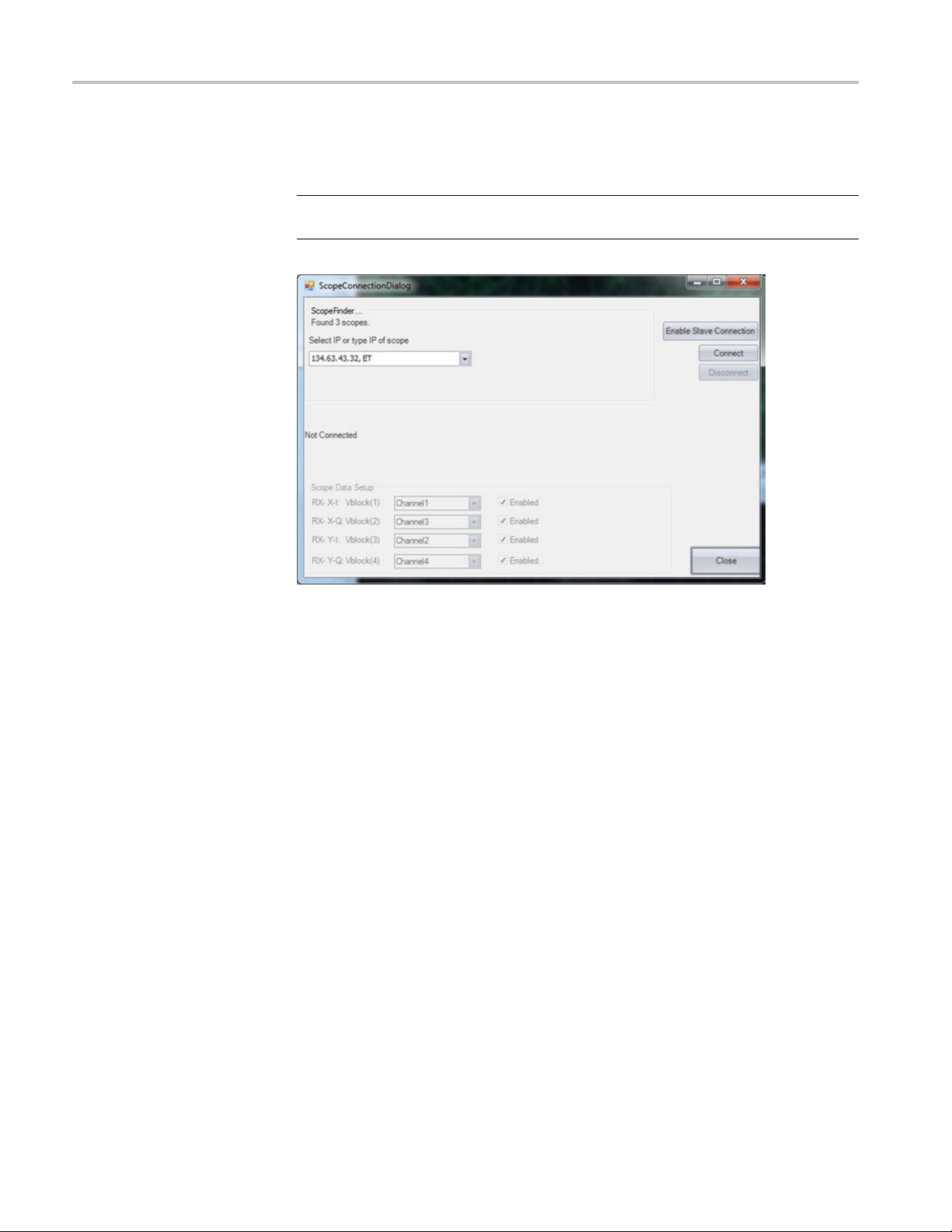
Conﬁguring the OM4000 user interface (OUI)

When connectin the box unless you require a VISA connection.

NOTE. Clicking Connect on the OUI Setup Tab opens the Scope Connection

dialog box for connecting to the Scope Service Utility.

g from the OUI, you will see a check box for VISA. Do not check

The green bar at the top indicates that the software is searching for oscilloscopes on the s they are added to the drop-down menu. If the OUI Scope Connection Dialog box reports 0 Scopes Found, you will have to type in the IP address manually. This happens when connecting over a VPN or when network policies prevent the IP broadcast. When typing the address in manually, do not include “, ET” or “, RT” on the end. Click Connect.

After connection, map the channels to the physical receiver channels and corresponding MATLAB variables as shown. This means that data from the sel X-Inphase, Vblock(2) is X-Quadrature, Vblock(3) is Y-Inphase, Vblock(4) is Y-Quadrature. The mapping you choose will depend on the cable connections made to the receiver.

ame subnet that are running the Scope Service Utility. As they are found

ected channel will be moved into the indicated Vblock variable. Vblock(1) is

60 OM4000D Series Coherent Lightwave Signal Analyzer

Conﬁguring the OM4000 user interface (OUI)

Once connected and conﬁgured, close the connect dialog box. The OUI is ready to use.

Two-oscilloscope conﬁguration

OUI Ver MSO/DSO70000C- or D-Series oscilloscopes are both connected to an OM4000. (See page 145, Conﬁguring two Tektronix 70000 series oscilloscopes.)

sions 1.5 and later support a conﬁguration where two Tektronix

OM4000D Series Coherent Lightwave Signal Analyzer 61

MATLAB

Launching the OUI also launches the installed MATLAB application.

The MATLAB default working directory is the installation directory. Use the cd command to change to another directory if desired. Any ﬁles saved will go to the working directory. Once the OUI is running, the MATLAB Command Window is populated w

ith the variables and functions used in coherent signal processing:

62 OM4000D Series Coherent Lightwave Signal Analyzer

Ta king measurements

Settingupyourmeasurement

Since the OM4000 is a reconﬁgurable (complex, dual-polarized) reference receiver, it requires a modulated signal on the input ﬁber. Depending on the options conﬁgured in the receiver, this modulation can be single- or dual-polarized, with several formats available, including OOK (on-off keying), BPSK (binar and either coherent or differential QAM and other formats are also available.

y phase-shift keying), and QPSK (quadrature phase-shift keying),

The OM4000 use these or your own lasers for signal and reference inputs. Furthermore, each polarization can be independently driven by a distinct source, though all sources must be tuned to the same ITLA channel, or at least to the same wavelength. While no phase locking of the sources is necessary, the beatnote between any signal laser and the reference should be at a low enough frequency that the ban bandwidth plus the beatnote frequency.

Befor lasers (i.e. that your data source [pattern generator] is not enabled). With both lasers emitting and tuned to the same channel, use the ﬁne-tune feature of the Laser/Receiver Control Panel to obtain a 100-500 MHz beat note on the oscilloscope. Then enable modulation, e.g. by activating your data source or pattern generator.

dwidth of the real-time oscilloscope can accommodate the modulation

e testing a modulated source, ensure that there is no modulation of the

includes two network-tunable sources (C- or L-band); you can

OM4000D Series Coherent Lightwave Signal Analyzer 63

Taking measurements

MATLAB Engine

ﬁle

You c an c o nﬁgure MATLAB to perform a wide range of mathematical operations on the raw or processed data using the Engine window. Normally the only c all is to CorePro recovery.

NOTE. To view a complete list of variables, open the MATLAB Command Window

and ent

cessingCommands, the set of routines performing phase and clock

er who.

NOTE. CoreProcessingCommands will provide either ET or RT processing

depending on which mode the OUI is in. To ensure you only get ET processing you can use CoreProcessingET in the window instead of CoreProcessingCommands. Similarly you can use CoreProcessing in the Engine Window if you want to be

you only get real-time processed data.

sure

As with all other settings, the last engine ﬁle used is recalled; you can locate

reate another appropriate engine ﬁle and paste it into the OUI MATLAB

or c window. Subsequent chapters explain in detail the operations of Core Processing. In addition to any valid MATLAB operations you may wish to use, there are some special variables that can be set or read from this window to control processing for a few special cases:

64 OM4000D Series Coherent Lightwave Signal Analyzer

Taking measurements

EqFiltInUse – a in use

pHybInUse – a s in use

DebugSave – analysis:

DebugSave =

ﬁles saved per block plus one ﬁnal save.

DebugSave

Click Si the connection. Use a short record length (for example, 2000 points) to speed up the display, click on Run-Stop to show continuously-updated measurements.

Using the Home tab, set up the plots you want, either using the stored Layout button or by clicking on the particular display format icon in the Plot Tools bar.

ngle and observe that the oscilloscope takes a burst of data; this conﬁrms

string which contains the properties of the equalization ﬁlter

tring which contains the properties of the optical calibration

logical variable that controls saving of detailed .mat ﬁles for

1 in the MATLAB Engine Command window results in two

= 0 or empty suppresses .mat ﬁle saves.

lays can be rearranged within the UI window or dragged and positioned

Disp randomly on the Windows Desktop. Clicking and dragging a window using its title tab brings up a positioning guide. Hold down the left mouse button to position the window onto the positioning guide, then release to organize the plots.

Constellation and Eye plots can be rescaled by clicking on the relevant scaling icons in the Controls tab of the left panel of the UI. The scale in √W/div is indicated.

Options for each plot are accessed by right-clicking on the plot. Trace and symbol contrast can be set globally using the sliders on the left bar of the OUI. Set trace and symbol properties for a particular plot using the right-click on the plot.

OM4000D Series Coherent Lightwave Signal Analyzer 65

Taking measurements

Multicarrier

support (MCS) option

The Multicarrier Setup

window

As network operators seek to increase the capacity of their ﬁber-optic transmission systems, moving wavelength division multiplexing (WDM) signals closer together is an attract using digital ﬁlters after coherent detection rather than more coarse WDM ﬁlters. This also simpliﬁes routing since more is under digital control.

A group of tightly packed WDM channels is sometimes called a superchannel because of the many channels. It is also known as a multicarrier signal since the various channels come from separately modulated carriers. In this document the term multicarrier refers to the group, where channel refers to an individual modulated carrier.

The optional MCS function displays the results of multiple channels within a multicarrier signal at the same time. The MCS option can scan automatically between OUI displays the results with the appropriate channel label by recognizing the channel based on the frequency entered by the user.

The Mu to start and stop an automatic scan, and to deﬁne which channels will be included in separate axis plots Multicarrier Eye and Multicarrier Constellation. The window is divided into two sections: Multicarrier channel list and Multicarrier display layout. The absolute channel list is shown on the right, the relative version on the left.

ive option. The densely packed signals are more readily separated

channels. Alternatively, the scan may be performed manually, and the

lticarrier Setup window allows the user to deﬁne the carrier channel plan,

When the MCS feature is enabled in the USB HASP key, the OUI displays the Mulitcarrier Setup button on the Setup ribbon.

Figure 5: Multicarrier Setup button (Home ribbon)

Click the Multicarrier Setup button to open the Multi Setup window.

66 OM4000D Series Coherent Lightwave Signal Analyzer

Taking measurements

Figure 6: Multicarrier setup window

Multicarrier channel List. The main part of this section is the channel deﬁnition

table. There are two types of channel deﬁnition table: absolute and relative. The default table type is absolute. A relative table m ay be entered by selecting Channel List Options: Add channel list: Add a new relative channel list. With an

ute channel deﬁnition table the channel frequencies speciﬁed are the actual

absol optical frequencies, in the region of 195 THz. If the table is relative then the frequencies refer to the difference between the channel frequency and the current local oscillator frequency. Relative frequencies are speciﬁed in gigahertz.

The absolute channel deﬁnition table has four columns:

The Channel column contains an integer identifying the channel. The values in this column do not have to be consecutive. The Frequency column contains the absolute channel frequency.

The Preferred LO is the frequency that the local oscillator (also called the Reference Laser) is tuned to during an automatic scan to observe that channel. If the bandwidth of the multicarrier channels are so large that only one channel can be observed at a time given the bandwidth of the oscilloscope, then the Preferred LO is typically set to the same value as Frequency. If the channels have smaller bandwidth, then several table rows may be set to the same Preferred LO (even though the Frequency is different) so that all those channels are captured at the same local oscillator setting. This can save time, because tuning the local oscillator may be slow.

OM4000D Series Coherent Lightwave Signal Analyzer 67

Taking measurements

The OUI identiﬁ frequency (in the Frequency column) and the LO frequency.

The ﬁnal colum scan. The relative channel deﬁnition table has only three columns. The second column, called Offset Frequency, contains the difference frequency between the channel and current local oscillator frequency.

NOTE. The terms “Reference Laser” and “Local Oscillator” (LO) are used

interchangeably in the OUI and LRCP. The term LO is used here and in the channel li

When the Add Channel button is pressed a new table row is added. The new entry has a Channel number one higher than the previous entry. The frequency columns contain thedifferencebetweenthepreviousrowand the row preceding that. The user is free to edit all the new row’s values. A table entry is removed by clicking on that row and pressing delete on the keyboard.

The user may enter several channel deﬁnition tables, and choose which one applies from the dropdown menu at the top left. A table may be deleted from the Channel List Options button.

st because it is more compact.

values that are incremented from the previous row by an amount equal to

es the channel by the difference between its absolute

n decides whether a channel will be included in the automatic

Multicarrier Plots

The Scan Single button and Scan Run-Stop buttons start single and continuous automatic scans respectively. The OUI may take many acquisitions at each LO setting during the automatic scan, accor ding to the Acquisitions per frequency

trol.

con

Multicarrier display layout. This section allows the user to specify which plots will appear in the separate axis plots, and how the subplots will be arranged. The Automatic layout checkbox (on by default) leaves the OUI to decide how to arrange the subplots. When Automatic layout is not checked, the region below

ecomes active. The user may choose the number of columns and rows of

b subplots either from the named controls, or by moving the horizontal and vertical sliders. Then the channel number to be plotted in each subplot is chosen from the dropdown menu.

A number of new plots have been added to the OUI for the MCS option. These plots are only available when the MCS feature is found on the USB HASP key. The common feature of the multicarrier plots and tables is that they store information from prior data acquisition.

Since the display is organized to show the performance of an entire channel group while analyzing one at a time, only one portion of the plot or table is updating while the rest retains its last data. Use the Clear Data button in the left-pane Controls group to clear all stored data.

68 OM4000D Series Coherent Lightwave Signal Analyzer

Taking measurements

Multicarrier s

pectrum. The Multicarrier Spectrum plot is accessed by clicking on

the spectrum icon button on the Home tab. Right-click on the plot to select what to display. By default the Input Signal spectrum is displayed. Each spectrum is labeled with its channel number appearing at its center frequency.

Figure 7: Multicarrier spectrum context menu

Table 13: Multicarrier spectrum menu choices (right-click)

Item Description

Input signal

After front-end proc

Front end ﬁlter Displays the digital ﬁlter transfer function speciﬁed in Analysis Parameters.

Subsequence average

After FE proc, X Poln

After FE proc, Y Poln

Multicarrier channels

Show new channels

Save graphics to PNG ﬁle

Displays the power spectrum of the input signal in dBW.

Displays the power spectrum after digital ﬁlter is applied as speciﬁed in Analysis Parameters.

A control is provided to adjust where the plot is placed since the units are relative, not dBW.

Displays the power spectrum of the averaged signal as calculated by the subsequence averaging function which is controlled by settings in Analysis Parameters.

Displays the power spectrum of the transmitter’s X-polarization signal after front-end processing.

Displays the power spectrum of the transmitter’s Y-polarization signal after front-end processing.

Choose which of the multicarrier channels to display.

Automatically display any new channels which are added to the Multicarrier channel list.

Saves the current plot to a PNG ﬁle.

OM4000D Series Coherent Lightwave Signal Analyzer 69

Taking measurements

Table 14: Multi

Item Description

Freq/Div Click the narr

Cent Freq Click the left arrow (spectrum left, higher center frequency) or right arrow

Ref dBW Use the +/- buttons to increase or decrease the power in dBW

dB/Div Click the

Absolute/ Relative

nter

Autoce

carrier spectrum controls

ow spectrum icon (narrower spectrum, more GHz/Div) or wide spectrum icon (wider spectrum, less GHz/Div) to change the horizontal frequency axis scale. Units are selectable via the drop-down menu but also Absolute/Relative/Autocenter choices.

(spectrum right, lower center frequency) to change the center frequency value one fu selectable via the drop-down menu but also change automatically when a change is made to the Absolute/Relative/Autocenter choices.

correspon

icon (shorter spectrum, more dB/Div) to change the vertical axis scale.

Click to toggle between Absolute and Relative (relative to current Reference Laser frequency) frequency axis modes. A 194 THz signal with a 193.99 Absolute mode and at 1 GHz in Relative mode.

Click to turn Autocenter on or off. With Autocenter on, all channels w ill be shifted to zero Hz center frequency to facilitate visual comparison.

change automatically when a change is made to the

lldivisionatatimeortypeinthevaluedirectly. Unitsare

ding to the top of the plot.

tall spectrum icon (taller spectrum, less dB/Div) or short spectrum

9 THz Reference Laser frequency will be displayed at 194THz in

Understanding the multicarrier spectrum plot.

Figure 8: Multicarrier spectrum plot

70 OM4000D Series Coherent Lightwave Signal Analyzer

Taking measurements

Like the other m each channel a nalyzed to form a composite view of the channel group. In the example shown above, this means that the Input Signal spectrum calculated while analyzing channel 1 is plotted in green together with that calculated while analyzing channel 2 in red. This scan was done with an absolute channel deﬁnition table.

Because a different LO frequency was speciﬁed for each channel, the red and green plots cover d ifferent spectral regions. When the LO was tuned to channel number 1, t the red spectrum. Since the channels are close together relative to the optical bandwidth of the system, there is substantial overlap between red and green. The red spectrum cuts off sharply on the left side corresponding to the lower limit of the optical system bandwidth whereas the green spectrum cuts off sharply on the right side corresponding to the upper edge of the optical system bandwidth for that

Ignoring the sharp cut-offs, the union of the red and green curves gives the true optica achieve in a single LO tuning.

LO tuning.

l spectrum which is wider than what the 23 GHz receiver used here could

ulticarrier plots, the Multicarrier Spectrum plot saves data from

he green spectrum was found. When it was tuned to channel 2 it was

OM4000D Series Coherent Lightwave Signal Analyzer 71

Taking measurements

Figure 9: Multicarrier spectrum plot details

The ﬁgure above shows some of the other features of the Multicarrier Spectrum plot. Here the X-pol signal after front-end processing is shown together with the digital ﬁlter used. Notice that the X-pol signal (purple or orange) show much deeper nulls than the total power spectrum (red or green). The nulls are the result of using a split and delay technique to generate the electrical I and Q modulator input signals from one data stream. There is a null at integer multiples of one over the difference in cable delays.

Since different cables are used on the X and Y inputs of the modulator, the nulls do not perfectly align and so wash out when looking at the total power spectrum. The nulls are clearly visible once the transmitter polarization signals have been

parated.

Multicarrier Constellation Plots. The Multicarrier Constellation plots are accessed by clicking on the constellation icon button on the Home tab. These plots behave in a similar fashion to the existing constellation plots except that there are regions reserved for each channel. The layout is controlled by the Multicarrier Setup window described above.

72 OM4000D Series Coherent Lightwave Signal Analyzer

Taking measurements

As each channel the most recent data displayed will continue to be shown in the other regions so that an aggregate view of the multicarrier group can be displayed. Use the Clear Data button to discard prior data.

Figure 10: Multicarrier constellation plots

Multicarrier Eye diagrams. The Multicarrier Eye Diagrams are accessed by

clicking on the Eye icon button on the Home tab. These plots behave in a similar fashion to the existing eye plots except that there are regions reserved for each channel. The layout is controlled by the Multicarrier Setup w indow described

above

is analyzed, only that portion of the plot will be updated while

As each channel is analyzed, only that portion of the plot will be updated while

ost recent data displayed will continue to be shown in the other regions so

the m that an aggregate view of the multicarrier group can be displayed. Use the Clear Data button to discard prior data.

OM4000D Series Coherent Lightwave Signal Analyzer 73

Taking measurements

Figure 11: Multicarrier Eye diagrams plot

EVM vs. Channel and Q vs. Channel. The EVM vs. Channel and Q vs. Channel

plots are accessed by clicking on the Q icon button on the Home tab. These plots

y the most recently measured EVM or Q factor for each channel. Only the

displa current channel will be updated while the most recent data displayed will continue to be shown for the other channels so that an aggregate plot of the multicarrier group can be displayed. Use the Clear Data button to discard prior data.

Figure 12: EVM vs. Channel plot

74 OM4000D Series Coherent Lightwave Signal Analyzer

Figure 13: Q vs. Channel plot

Taking measurements

Measurem

clicking on the tabular data icon on theHometab. Thistableissimilartothe Measurement Statistics table except that only the most recent value is shown so that data from every channel can be displayed in one plot. As with the Measurement Statistics plot, it is necessary to make sure the desired measurement is enabled in the Analysis Parameters since some measurements are not calculated unles

ent vs. Channel. The Measurement vs. Channel table is accessed by

sspeciﬁcally enabled.

Figure 14: Meas vs. Channel table

OM4000D Series Coherent Lightwave Signal Analyzer 75

Taking measurements

76 OM4000D Series Coherent Lightwave Signal Analyzer

Tektronix OM4106D, OM4006D User Manual

Specifications and Main Features

Frequently Asked Questions

User Manual

Important safety information

General safety summary

ice procedures. Read this Service safety summary and the General safety

Terms in this manual

Symbols and terms on the product

Compliance information

EMC compliance

Environmental considerations

Preface

Supported products

About this manual

Getting started

Product description

Accessories

Options

Initial product inspection

Environmental operating requirements

Power requirements

Equipment setup

Operating basics

Software overview

The Laser Receiver Control Panel (LRCP) user interface

The OM4000 user interface (OUI)

Non-VISA oscilloscope connections (Scope Service Utility)

MATLAB

Ta king measurements

Settingupyourmeasurement

Taking measurements