

Page 1

xx
OM1106, OM4006, OM4106
ZZZ
Coherent Lightwave Signal Analyzer
User Guide
*P071316000*
071-3160-00
Page 2

Page 3

xx
OM1106, OM4006, OM4106
ZZZ
Coherent Lightwave Signal Analyzer
User Guide
www.tektronix.com
071-3160-00
Page 4

Copyright © Tektronix. All rights reserved. Licensed software products are owned by Tektronix or its subsidiaries
or suppliers, and are protected by national copyright laws and international treaty provisions.
Tektronix products are covered by U.S. and foreign patents, issued and pending. Information in this publication
supersedes that in all previously published material. Specifications and price change privileges reserved.
TEKTRONIX and TEK are registered trademarks of Tektronix, Inc.
Contacting Tektronix
Tektronix, Inc.
14150 SW Karl Braun Drive
P.O. B o x 5 0 0
Beaverto
USA
For product information, sales, service, and technical support:
n, OR 97077
In North America, call 1-800-833-9200.
Worl dwid e, vis it www.tektronix.com to find contacts in your area.
Page 5

Warranty
Tektronix warrants that this product will be free from defects in materials and workmanship for a period of one (1)
year from the date of shipment. If any such product proves defective during this warranty period, Tektronix, at its
option, either will repair the defective product without charge for parts and labor, or will provide a replacement
in exchange for the defective product. Parts, modules and replacement products used by Tektronix for warranty
work may be n
the property of Tektronix.
ew or reconditioned to like new performance. All replaced parts, modules and products become
In order to o
the warranty period and make suitable arrangements for the performance of service. Customer shall be responsible
for packaging and shipping the defective product to the service center designated by Tektronix, w ith shipping
charges prepaid. Tektronix shall pay for the return of the product to Customer if the shipment is to a location within
the country in which the Tektronix service center is located. Customer shall be responsible for paying all shipping
charges, duties, taxes, and any other charges for products returned to any other locations.
This warranty shall not apply to any defect, failure or damage caused by improper use or improper or inadequate
maintenance and care. Tektronix shall not be obligated to furnish service under this warranty a) to repair damage
result
b) to repair damage resulting from improper use or connection to incompatible equipment; c) to repair any damage
or malfunction caused by the use of non-Tektronix supplies; or d) to service a product that has been modified or
integrated with other products when the effect of such modification or integration increases the time or difficulty
of servicing the product.
THIS WARRANTY IS GIVEN BY TEKTRONIX WITH RESPECT TO THE PRODUCT IN LIEU OF ANY
OTHER WARRANTIES, EXPRESS OR IMPLIED. TEKTRONIX AND ITS VENDORS DISCLAIM ANY
IMPLIED WARRANTIES OF MERCHANTABILITY OR FITNESS FOR A PARTICULAR PURPOSE.
TRONIX' RESPONSIBILITY TO REPAIR OR REPLACE DEFECTIVE PRODUCTS IS THE SOLE
TEK
AND EXCLUSIVE REMEDY PROVIDED TO THE CUSTOMER FOR BREACH OF THIS WARRANTY.
TEKTRONIX AND ITS VENDORS WILL NOT BE LIABLE FOR ANY INDIRECT, SPECIAL, INCIDENTAL,
OR CONSEQUENTIAL DAMAGES IRRESPECTIVE OF WHETHER TEKTRONIX OR THE VENDOR HAS
ADVANCE NOTICE OF THE POSSIBILITY OF SUCH DAMAGES.
[W2 – 15AUG04]
btain service under this warranty, Customer must notify Tektronix of the defect before the expiration of
ing from attempts by personnel other than Tektronix representatives to install, repair or service the product;
Page 6

Page 7

Table of Contents
1 SAFETY INFORMATION ...................................................................................................................... 7
1.1 SAFETY NOTICES ............................................................................................................................. 7
1.2 LASER SAFETY ................................................................................................................................. 7
1.3 OM4000 SERIES LASER LABELS AND LOCATIONS .............................................................................. 8
2 INTRODUCTION ................................................................................................................................... 9
2.1 PURPOSE ......................................................................................................................................... 9
3 GETTING STARTED ........................................................................................................................... 10
3.1 CONFIGURING THE HARDWARE ....................................................................................................... 10
3.2 OVERVIEW AND CONFIGURATION OF THE SOFTWARE ....................................................................... 19
4 MAKING MEASUREMENTS ............................................................................................................... 43
4.1 SETTING UP YOUR MEASUREMENT ................................................................................................. 43
4.2 ENGINE FILE ................................................................................................................................... 43
4.3 PERFORMING MEASUREMENTS ........................................................................................................ 44
5 USING THE OUI .................................................................................................................................. 46
5.1 OUI OVERVIEW .............................................................................................................................. 46
5.2 ANALYSIS PARAMETERS ................................................................................................................. 48
5.3 CONSTELLATION DIAGRAMS ............................................................................................................ 54
5.4 EYE DIAGRAMS .............................................................................................................................. 57
5.5 SIGNAL VS. TIME ............................................................................................................................. 58
5.6 WAVEFORM AVERAGING ................................................................................................................. 59
5.7 MEASUREMENTS ............................................................................................................................ 61
5.8 POINCARÉ SPHERE ........................................................................................................................ 62
5.9 BIT-ERROR-RATE REPORTING ........................................................................................................ 63
5.10 PMD MEASUREMENT ...................................................................................................................... 63
5.11 RECORDING AND PLAYBACK ........................................................................................................... 64
5.12 ALERTS ......................................................................................................................................... 65
5.13 MANAGING DATA SETS WITH RECORD LENGTH > 1,000,000 ............................................................ 67
6 LASER / RECEIVER CONTROL PANEL ............................................................................................ 70
6.1 DEVICE SETUP AND AUTO CONFIGURE ............................................................................................ 70
6.2 CONFIGURATION ON A NETWORK USING DHCP ................................................................................ 71
6.3 CONFIGURATION ON A NETWORK WITH NO DHCP ............................................................................ 72
6.4 CONNECTING TO YOUR OM4000 SERIES DEVICE ............................................................................. 75
Tektronix OM4006/OM4106 Coherent Lightwave Signal Analyzer User Guide V1.5.1 10/24 ©2012 Page 4 of 148
Page 8

6.5 SETTING LASER PARAMETERS ......................................................................................................... 77
7 ATE (AUTOMATED TEST EQUIPMENT) INTERFACE ..................................................................... 79
7.1 LRCP ATE INTERFACE .................................................................................................................. 79
7.2 OUI4006 ATE INTERFACE ............................................................................................................. 85
7.3 ATE FUNCTIONALITY IN MATLAB ................................................................................................... 91
7.4 BUILDING AN OM4006 ATE CLIENT IN VB.NET .............................................................................. 93
8 MAINTENANCE AND CLEANING .................................................................................................... 102
9 DETAILED CONFIGURATION OF EXPERIMENTS ......................................................................... 103
10 CORE PROCESSING SOFTWARE GUIDE ................................................................................. 105
10.1 INTERACTION WITH OUI ................................................................................................................ 105
10.2 MATLAB VARIABLES ...................................................................................................................... 106
10.3 MATLAB FUNCTIONS ..................................................................................................................... 107
10.4 SIGNAL PROCESSING STEPS IN COREPROCESSING ........................................................................ 107
10.5 BLOCK PROCESSING ..................................................................................................................... 113
10.6 ALERTS MANAGEMENT .................................................................................................................. 114
11 CORE PROCESSING FUNCTION REFERENCE ........................................................................ 116
11.1 ALIGNTRIBS ................................................................................................................................. 116
11.2 APPLYPHASE ............................................................................................................................... 119
11.3 CLOCKRETIME ............................................................................................................................. 120
11.4 DIFFDETECTION ........................................................................................................................... 121
11.5 ESTIMATECLOCK .......................................................................................................................... 123
11.6 ESTIMATEPHASE .......................................................................................................................... 125
11.7 ESTIMATESOP ............................................................................................................................. 127
11.8 MASKCOUNT ................................................................................................................................ 128
11.9 GENPATTERN .............................................................................................................................. 129
11.10 JONES2STOKES ....................................................................................................................... 130
11.11 JONESORTH ............................................................................................................................. 131
11.12 LASERSPECTRUM ..................................................................................................................... 132
11.13 QDECTH .................................................................................................................................. 133
11.14 ZSPECTRUM ............................................................................................................................. 135
12 MATLAB VARIABLES USED BY CORE PROCESSING .............................................................. 136
13 APPENDIX A – ADVANCED USE CASES ................................................................................... 137
13.1 CONFIGURING TWO 70000 SERIES OSCILLOSCOPES ...................................................................... 138
Tektronix OM4006/OM4106 Coherent Lightwave Signal Analyzer User Guide V1.5.1 10/24 ©2012 Page 5 of 148
Page 9

14 APPENDIX B: SOFTWARE LICENSE AGREEMENT .................................................................. 144
15 APPENDIX C – GLOSSARY OF TERMS ..................................................................................... 148
Tektronix OM4006/OM4106 Coherent Lightwave Signal Analyzer User Guide V1.5.1 10/24 ©2012 Page 6 of 148
Page 10

1 Safety Information
CAUTION
CAUTION
!
WARNING
!
!
CAUTION
!
1.1 Safety Notices
Indicates a potentially hazardous condition or procedure that could result in damage to the
instrument.
Indicates a potentially hazardous condition or procedure that could result in minor or moderate
bodily injury.
Indicates a potentially hazardous condition or procedure that could result in serious injury or death.
This symbol on the unit indicates that the user should consult this document for further
information regarding the nature of the potential hazard and actions that should be
taken to avoid or mitigate the hazard.
1.2 Laser Safety
The laser sources included in this product are classified according to
IEC/EN 60825-1: 1994+A1:2001+A2:2001 and IEC/EN 60825-2:2004
This laser product complies with 21CFR1040.10 except for deviations pursuant to
Laser Notice No. 50, dated June 24, 2007.
Use of controls or adjustments or performance of procedures other than those specified
herein may result in hazardous radiation exposure. Under no circumstances should you
use any optical instruments to view the laser output directly.
Additional laser safety notifications appear in the OM4000 Series User Interface (OUI) control
software section.
Tektronix OM4006/OM4106 Coherent Lightwave Signal Analyzer User Guide V1.5.1 10/24 ©2012 Page 7 of 148
Page 11

1.3 OM4000 Series Laser Labels and Locations
INVISIBLE LASER RADIATION; DO NOT VIEW DIRECTLY WITH
OPTICAL INSTRUMENTS: CLASS 1M LASER PRODUCT
EMISSION DE RAYONS LASER INVISIBLES DE CLASSE 1M.
NE PAS OBSERVER A L’AIDE D’INSTRUMENTS OPTIQUES
Indicates the
location of a
laser aperture
Model
MAC Address
Under top Cover:
Serial Number
Manufactured
Tektronix OM4006/OM4106 Coherent Lightwave Signal Analyzer User Guide V1.5.1 10/24 ©2012 Page 8 of 148
Page 12

2 Introduction
1
2
2.1 Purpose
The OM4000 Series Coherent Lightwave Signal Analyzer is a sophisticated, general-purpose
long-haul (C and L-band capable) fiber optics communications receiver that measures the
complete electric field (vs. time) in single-mode optical fiber. The system consists of the
Complex Modulation Receiver, Core Processing, and the OM4000 Series User Interface (OUI),
further incorporating a customer-supplied real-time 2- or 4-channel oscilloscope and external
computer, with the option for some oscilloscopes to run the OUI on the oscilloscope itself.
The Coherent Lightwave Signal Analyzer runs a Matlab1-based script, CoreProcessing, to
recover the phase of the complex-modulated lightwave signal and display the demodulated
result in several useful formats, such as eye diagrams of the tributaries, phase diagrams
(constellations) and the Poincaré sphere. This method offers access to the entire variable space
in Matlab, enabling you to change the order of processing, define new functions, and interact
with other programs, such as LabVIEW2.
MATLAB® is a registered trademark of The MathWorks, Inc. Other product and company names listed are
trademarks and trade names of their respective companies.
LabVIEW is a trademark of National Instruments, Inc.
Tektronix OM4006/OM4106 Coherent Lightwave Signal Analyzer User Guide V1.5.1 10/24 ©2012 Page 9 of 148
Page 13

3 Getting Started
3.1 Configuring the Hardware
3.1.1 OM4000 Series Receiver
Ensure that the required power sources for the OM4000 Series (100, 115 or 230 VAC, 50–60
Hz, 0.4 A), the associated oscilloscope, and the external computer (if used) are available.
The OM4000 Series Coherent Modulation Receiver, along with proprietary software comprises
the OM4000 Series Coherent Lightwave Signal Analyzer (CLSA). This system is used in
laboratory or industrial facilities to analyze next-generation complex-modulation fiber-optic data
signals. In operation, one of the receiver’s two laser outputs will be connected to one of the
optical input connectors (the reference, or local oscillator, input), and the second laser output
will be connected to the user’s device under test.
Note: The reference connection may optionally be configured internally at the factory.
The signal to be analyzed is connected to the “Signal” optical input. Four coaxial cables connect
the OM4000 Series to a high-speed sampling oscilloscope. An Ethernet connector will connect
the receiver, via a router, to a computer and to the oscilloscope. An IEC power cord is
connected to a rack or wall outlet. The OM4000 Series User Interface running on the computer
controls the OM4000 Series and the oscilloscope.
Note: A password is required to turn on the lasers through the Laser / Receiver Control Panel.
The default is ‘1234’
Associated cabling includes the power cord, an Ethernet cable, four coaxial cables (9 to 12
inches in length), and two fiber optic cables to connect the laser output and user’s signal to the
optical inputs.
Tektronix OM4006/OM4106 Coherent Lightwave Signal Analyzer User Guide V1.5.1 10/24 ©2012 Page 10 of 148
Page 14
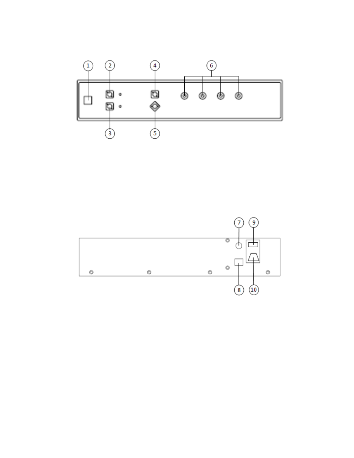
3.1.2 OM4000 Series Controls and I/O Connections
Front Panel Controls and I/O Connectors
1. On/Off switch
2. Laser 1 Output (with LED indicator)
3. Laser 2 Output (with LED indicator) (may be internally connected at the factory)
4. Input 1 (Signal input)
5. Input 2 (Reference input; may be internally connected at the factory)
6. RF connectors, to connect to the oscilloscope
Rear Panel Controls and I/O Connectors
7. BNC connector for optional laser remote interlock
8. Ethernet port
9. Fuse drawer
10. Input power receptacle
Tektronix OM4006/OM4106 Coherent Lightwave Signal Analyzer User Guide V1.5.1 10/24 ©2012 Page 11 of 148
Page 15
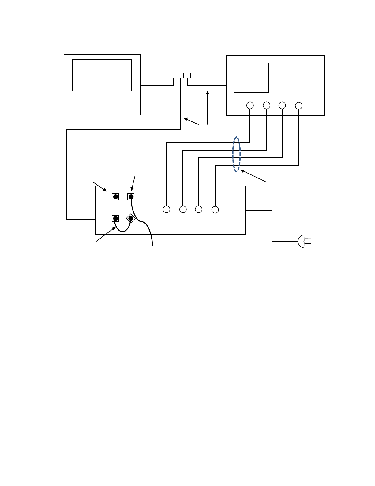
L1
L2
Computer –
PC or laptop
4-channel
Coaxial cables (4),
Fiber optic
Power cord
Ethernet
OM4000
Laser
outputs (2)
Optical
inputs (2)
IN1
IN2
To user’s
DUT
Gigabit
Switch
1 2 3 4
XI XQ YI YQ
patch cable
oscilloscope
6 -12 in. long typ.
Block diagram
3.1.3 List of Components
OM4000 Series Complex Modulation Receiver
IEC power cable
Ethernet cable
BNC shorting cap for interlock
(4) Dust covers for optical inputs not in use
(4) SMA caps to protect electrical outputs
Short PM patch cable to connect Laser 2 to Reference input
Short coaxial cables shaped to connect OM4000 Series outputs to oscilloscope inputs
Additional items needed, not part of Receiver:
Supported Oscilloscope (1 of the following)
o Real-time Tektronix Oscilloscope with at least 20 GS/s sampling rate on two or four
channels in the 70000 Series
o Equivalent-Time Tektronix Oscilloscope DSA8300 or DSA8200 with supported
sampling heads. See data sheet for supported samplers
Tektronix OM4006/OM4106 Coherent Lightwave Signal Analyzer User Guide V1.5.1 10/24 ©2012 Page 12 of 148
Page 16

Power cable
WARNING
!
WARNING
!
CAUTION
!
Ethernet cable
Mouse and keyboard (unless touch-screen controlled)
System controller PC running Windows 7 or XP, Matlab, the OM4000 Series User
Interface (OUI) software, and the Laser Receiver Control Panel (LRCP) software.
o Monitor plus cable
o Mouse and keyboard
o Power cables
o Ethernet cable
An Ethernet switch or hub plus a router running DHCP, and associated cabling (not shown)
Equipment for calibration as needed (see Calibration section)
OMRACK, 19” rack, or other method of ensuring OM4000 Series and oscilloscope are
securely stacked
To avoid the possibility of electrical shock, do not connect your OM4000 to a power
source if there are any signs of damage to the instrument enclosure.
3.1.4 Electrical Power Requirements
The OM4000 Series can operate from any AC power source that provides 100, 115, or 230
VAC, at a frequency of 60 Hz or 50 Hz respectively with a 0.4A rating. (The US rack-mount
system has a power connector that requires the special 20 A outlet configuration.) The OM4000
Series must be connected directly to a grounded power outlet only.
The OM4000 Series must be connected to a 100, 115, or 230VAC at 60Hz or 50Hz
respectively grounded outlet only. Operating the OM4000 Series without connection to a
grounded power source could result in serious electrical shock. Always connect the unit
directly to a grounded power outlet.
Protective features of the OM4000 Series may be impaired if the unit is used in a manner
not specified by Tektronix.
Tektronix OM4006/OM4106 Coherent Lightwave Signal Analyzer User Guide V1.5.1 10/24 ©2012 Page 13 of 148
Page 17

3.1.5 Location and Positioning
CAUTION
If the OM4000 Series is to be used in an installation other than a standard 19” rack, be sure to
position the unit so that the power switch at the rear of the unit can be easily accessed.
Be sure not to obstruct the fan so that there is an adequate flow of cooling air to the
electronics compartment whenever the unit is operating.
3.1.6 Operating Environment
The OM4000 Series may be operated within the following conditions:
Temperature 10°C to +35°C (50°F to +95°F)
Humidity <85% R.H. non-condensing from 10°C to +35°C (50°F to +95°F)
Altitude < 2,000 m (6560ft)
3.1.7 Computer
Install software on target computer and Oscilloscope.
See Installation Instructions
Mathworks MATLAB is required but not included in the install package.
Windows 7 64-bit Operating System: Install Matlab 2011b
Windows XP 32-bit Operating System: Install Matlab 2009a 32-bit
Recommended and Minimum Computer Requirements:
Operating System: US Windows-7 64 bit OR US Windows XP Service Pack 3 32-bit (.NET 4.0
required),
Processor: recommended: Intel I7, i5 or equivalent; min clock speed 2 GHz; minimum:
Intel Pentium 4 or equivalent,
RAM: min: 4 GB, For 64-bit releases will benefit from as much memory as is
available
Hard Drive Space: At least 300 GB recommended for large data sets; minimum: 20 GB,
Video Card: nVidia dedicated graphics board w/ 512+ MB min. graphics memory
Note: Color grade display feature is not available on non-nVidia graphics
cards and so will not be available when running native on an oscilloscope
Networking: Gigabit Ethernet (1 Gb/s) or Fast Ethernet (100Mb/s)
Display: 20” min, Large flat screen recommended for displaying multiple graph types
Tektronix OM4006/OM4106 Coherent Lightwave Signal Analyzer User Guide V1.5.1 10/24 ©2012 Page 14 of 148
Page 18

Other Hardware: DVD Optical drive, 2 USB 2.0 ports
Other Software: Computer must have Matlab installed according to instructions above.
Adobe PDF Reader is required for viewing the User Guide and Installation
instructions.
Tektronix OM4006/OM4106 Coherent Lightwave Signal Analyzer User Guide V1.5.1 10/24 ©2012 Page 15 of 148
Page 19
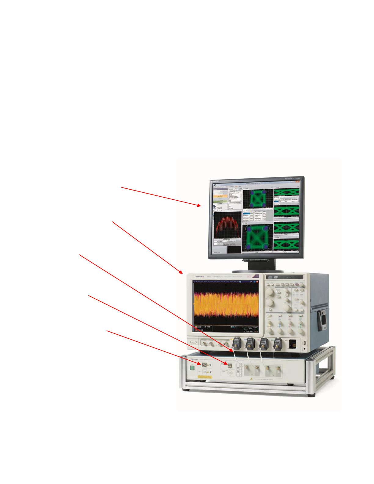
3.1.8 First Setup
Real time oscilloscope
RF interconnects
Signal-Laser Fiber Optic
System controller can be Win 7
Input signal SM APC
(from DUT)
System controller monitor or
Once everything is securely placed, make electrical connections in the following order:
1. Ethernet connections and other computer connections. See Section 3.1.2
2. Power connections from the OM4000 Series to the rack
3. Power from rack to mains (keeping main front panel switch off)
4. RF connections (the four coaxial cables from OM4000 Series to oscilloscope)
5. Fiber optic PM patch cable connection from Laser 2 to Reference (if needed)
6. Fiber optic Signal input connection (with no optical power present at setup)
7. Store all dust covers and coaxial connector caps for future use.
second monitor for Win 7
oscilloscope
PM APC output (if needed)
for DUT
oscilloscope or separate PC.
Separate PC required for certain
display options.
Tektronix OM4006/OM4106 Coherent Lightwave Signal Analyzer User Guide V1.5.1 10/24 ©2012 Page 16 of 148
Typical system configuration
Page 20

Once the equipment is positioned and connected, turn on the computer, the oscilloscope and
the main power switch on the back of the OM4000 Series. The OM4000 Series front-panel
power button will light briefly after main power is applied indicating it is searching for a DHCP
server. When an IP address has been assigned or when the search fails in the case of an
isolated network, the power light will go off. Press the power button one time to enable the unit.
The steady power button light indicates the OM4000 Series is ready for use and that lasers may
be activated at any time if a user connects via the Ethernet connection. The light will go out and
the unit will be disabled any time ac power is removed or the IP address is changed. Press the
power button to re-enable. This feature prevents a remote user from activating the lasers when
the local user may not be ready.
Note: Ethernet only allows devices on the same subnet to communicate.
You should now have three devices on an Ethernet network: computer, oscilloscope, and
OM4000 Series. This little network may be connected to your corporate network or router or you
may choose to leave it isolated. IP setup is normally done by at the time of installation. You
should only need the following instructions if you are reconfiguring your network.
3.1.8.1 IP setup on a network with DHCP (dynamic IP assignment)
DHCP allows “automatic” assignment of the IP address the connected devices need to
communicate with each other. However, automatic IP assignment must be selected on each
device before this will be allowed. The OM4000 Series is shipped with automatic IP assignment
enabled. Your computer and oscilloscope may need this turned on.
Once automatic IP assignment is selected, you may still need the cooperation of your corporate
IT department to get IP addresses assigned. If you are using a centralized server, ask your
network administrator to make an IP reservation for you so that you get the same number each
time the device is powered on. Once these are set up for the oscilloscope and the OM4000
Series you will have no trouble finding them in the future.
Once your equipment gets an IP address from DHCP you can find that address using the
operating system of the oscilloscope or computer. For example, in the XP operating system
there is a window that looks like the one below. Notice that when you select the active Ethernet
connection the IP address shows up in the Details box in the lower-left corner of the window.
To configure the IP connection of the OM4000 Series receiver, please see Chapter 6 on using
the Laser Receiver Control Panel (LRCP).
Tektronix OM4006/OM4106 Coherent Lightwave Signal Analyzer User Guide V1.5.1 10/24 ©2012 Page 17 of 148
Page 21

3.1.8.2 IP setup on an isolated network or one not running a DHCP server
When there is no DHCP server, the Ethernet connected devices don’t know what address to
assign to themselves. In this case you must manually set the IP address. On a corporate
network this means getting the IP addresses from your network administrator first and then
setting each device. Your network administrator may need the MAC addresses of the computer,
oscilloscope, and OM4000 Series. The MAC address for your OM4000 Series box is located on
the rear panel label. On newer models the MAC address is printed on the real-panel label. See
Section 6.3 for instructions to set the OM4000 Series IP address. If you have a network isolated
from your corporate network you are free to use any IP numbering scheme. Tektronix
recommends 172.17.200.XXX where XXX is any unique number between 0 and 255 (each
device needs a unique number). There is nothing special about this scheme other than that it is
the default for new OM4000 Series units. Use the operating systems of the oscilloscope and
computer to set their IP addresses. The first three sets of numbers in the IP address need to be
the same on the computer and the connected devices for them to communicate in most cases.
Note: For setup purposes, to ease communication between the LRCP and the controller com-
puter, be sure the controller computer (e.g. laptop) has only one Ethernet medium (e.g.
wireless or wired) activated
Tektronix OM4006/OM4106 Coherent Lightwave Signal Analyzer User Guide V1.5.1 10/24 ©2012 Page 18 of 148
Page 22

3.2 Overview and Configuration of the Software
OM4000 Series
User Interface
(OUI)
Matlab
IVI/Visa OR
Scope Service
Oscilloscope
Laser/Receiver
Control Panel
(LRCP)
OM4000 Series
Hardware
The OM4000 Series Software includes the OM4000 Series User Interface (OUI) and the Laser/
Receiver Control Panel (LRCP). The LRCP controls the hardware and communicates with the OUI
which is the primary user interface. The OUI collects data from the user, the LRCP, and the
oscilloscope and communicates with the Matlab Engine to input data and collect finished
calculations. The OUI can also communicate with customer applications via the Windows
Communication Foundation (WCF) interface described in Chapter 7.
Tektronix OM4006/OM4106 Coherent Lightwave Signal Analyzer User Guide V1.5.1 10/24 ©2012 Page 19 of 148
Page 23
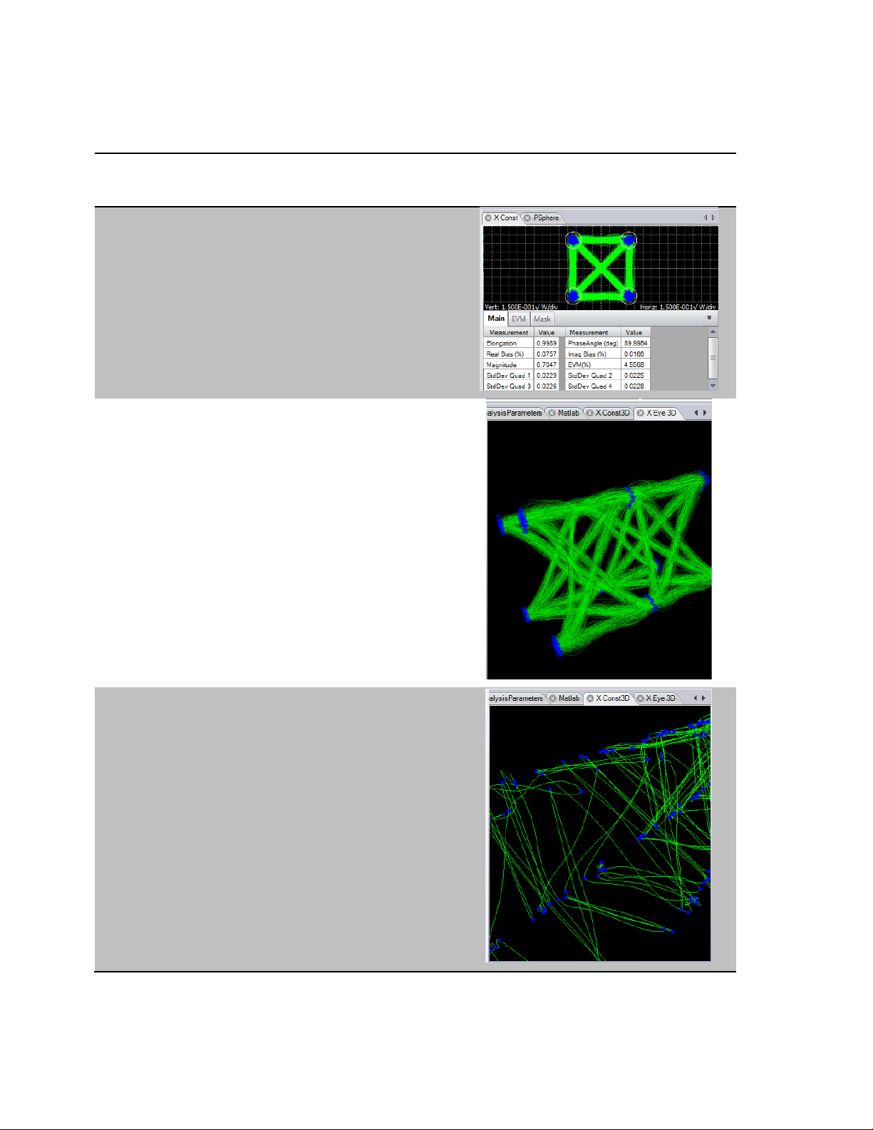
3.2.1 Summary of Plots and Measurements in the OUI
Description
Plot available with Real-time
Oscilloscope
Constellation Diagram for X or Y signal
polarization with numerical readout bottom tabs.
Right-click to see graphics options
Symbol-center values are shown in blue
Symbol errors are shown in red
Right-click for other color options
3d Eye for X or Y signal polarization.
This plot can be scaled and rotated to view on a
2d or 3d monitor. It shows the Constellation
Diagram with a time axis modulo two bit periods.
3d Constellation for X or Y signal polarization.
This plot can be scaled and rotated to view on a
2d or 3d monitor. It shows the Constellation
Diagram with a time axis.
Tektronix OM4006/OM4106 Coherent Lightwave Signal Analyzer User Guide V1.5.1 10/24 ©2012 Page 20 of 148
Page 24
The coherent eye diagram for X or Y signal
polarization shows the In-Phase or Quadrature
components vs. time modulo two bit periods.
The Q-factor results are provided in a tab below
accessed by clicking on the arrows in the lower
left corner.
Right-click on the coherent eye diagram to get
options including transition and eye averaging.
The transition average shown in red is an
average of each logical transition. The
calculation is enabled in the Analysis Parameters
tab and is used for calculating transition
measurements.
The Power Eye shows the computed power per
polarization vs time modulo 2 bit periods. This is
a calculation of the eye diagram typically
obtained with a photodiode-input oscilloscope.
Most plots can be viewed in colorgrade by rightclicking on the plot.
Right-click on the X vs T plot to display field,
averaged-field, and symbol quantities. Zoom in
or out or scroll through the record. Error
symbols are shown in red.
BER is shown by physical tributary and in total.
Color changes on synch loss.
Tektronix OM4006/OM4106 Coherent Lightwave Signal Analyzer User Guide V1.5.1 10/24 ©2012 Page 21 of 148
Page 25
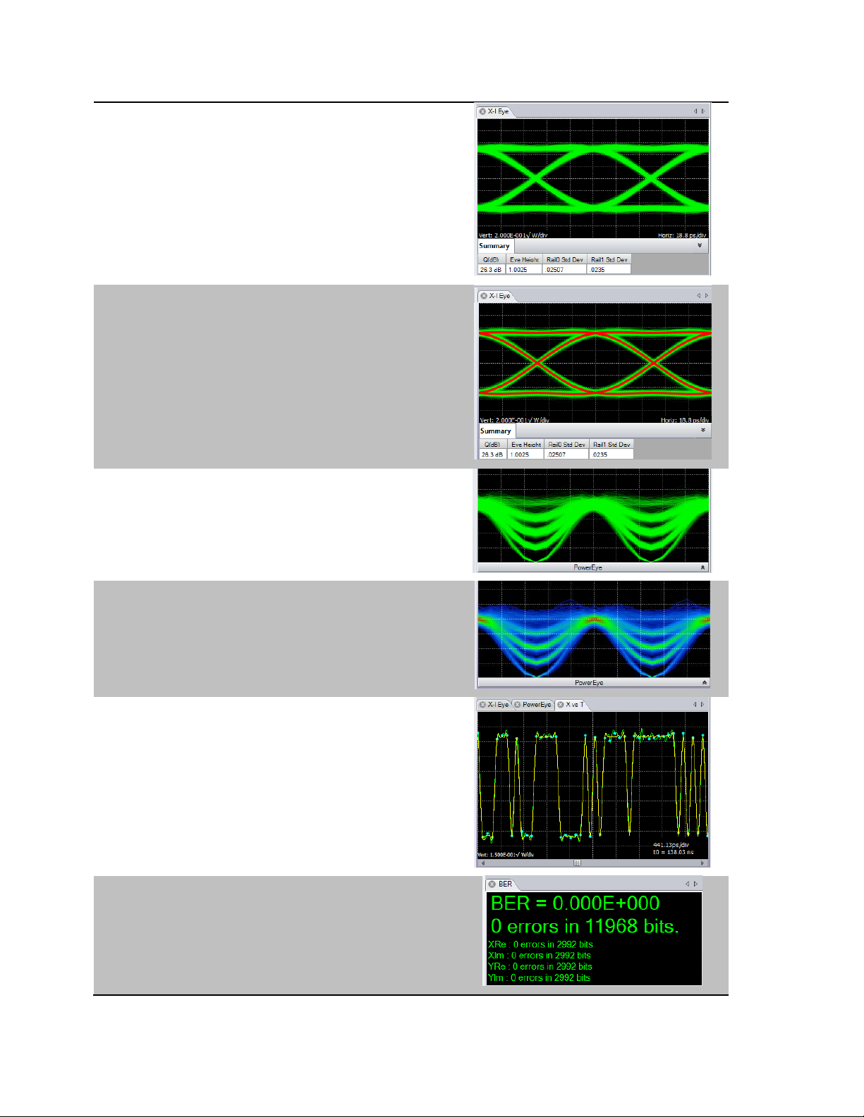
2d Poincare shows the position of the data
signal polarizations relative to the receiver’s H
(1, 2) and V (3, 4).
3d Poincare shows polarization of each symbolcenter value.
Click and drag to rotate the sphere.
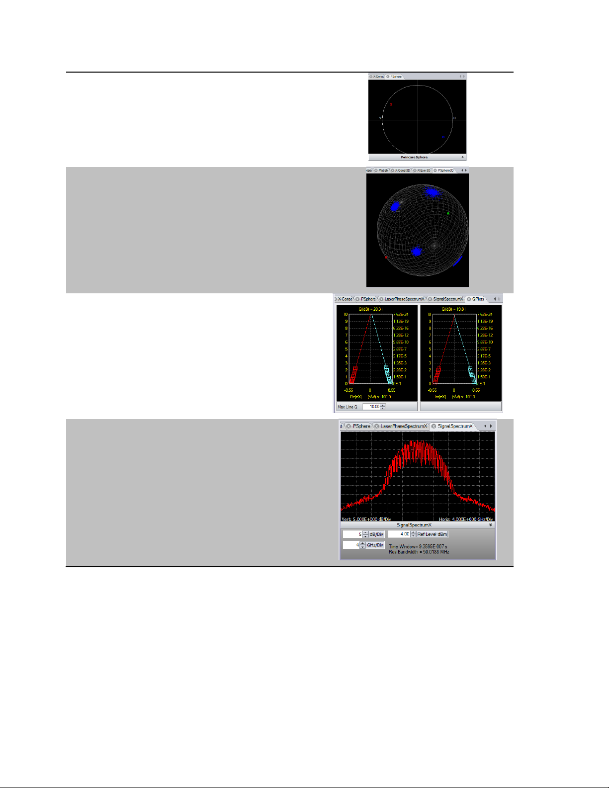
The Decision-Threshold Q-Factor is an ideal
signal quality measurement based on measured
BER values. The horizontal axis corresponds to
the vertical axis on the corresponding coherent
eye plot. Linear Q is on the left and BER on the
right of the plot. Measured values are indicated
by squares: blue for 1’s red for 0’s.
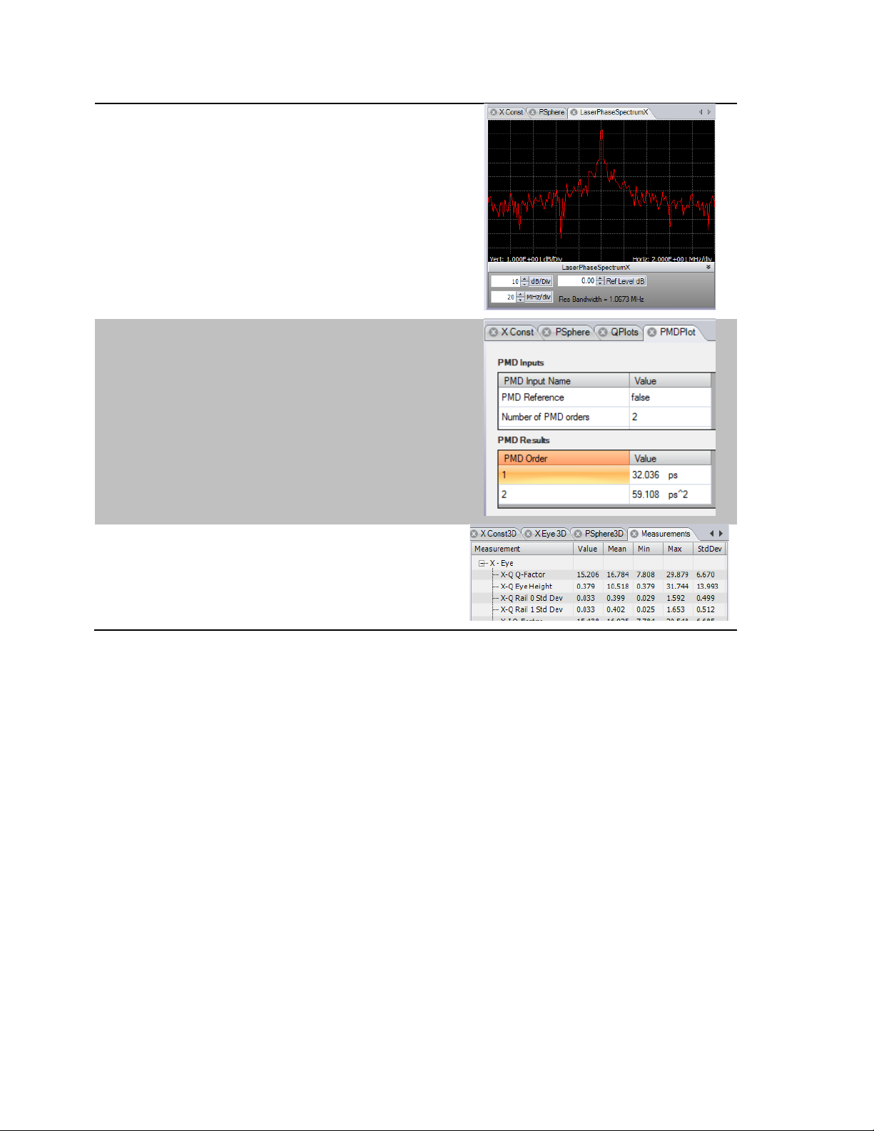
The frequency spectrum of the signal field is
calculated using an FFT after polarization
separation to obtain the spectrum of each signal
polarization.
Tektronix OM4006/OM4106 Coherent Lightwave Signal Analyzer User Guide V1.5.1 10/24 ©2012 Page 22 of 148
Page 26
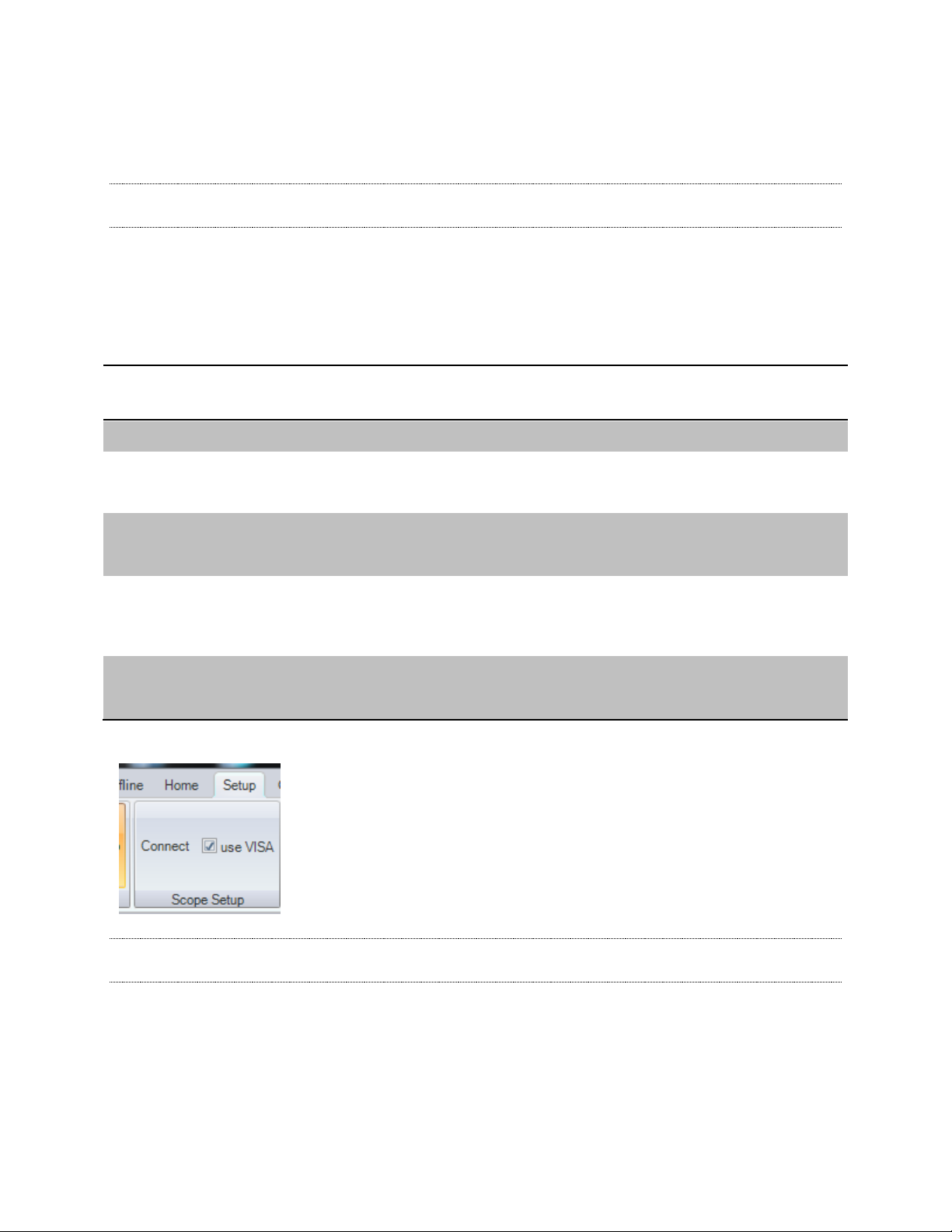
The laser phase noise spectrum is obtained by
taking an FFT of the where ϴ is the recovered
laser phase vs. time.
The PMDPlot provides the results of the PMD
Calculation
The Measurements Tab provides a convenient
place to find almost all of the numerical outputs
provided by the OUI with statistics on each
value.
Tektronix OM4006/OM4106 Coherent Lightwave Signal Analyzer User Guide V1.5.1 10/24 ©2012 Page 23 of 148
Page 27
3.2.3 Configuring the OM4000 Series User Interface (OUI)
VISA
Non-VISA Scope
Service Utility
Segmented readout for unlimited record size
YES
YES
Ability to collect data from two networked
oscilloscopes running the Scope Service
NO
YES
Software required on oscilloscope
LAN Server
Scope Service Utility or
ET Scope Service Utility
Real-time oscilloscope compatibility
Any real-time Tektronix
oscilloscope supported
by the IVI driver
C and D-model 70000
Series Oscilloscopes
with v6.4 firmware
Equivalent-time oscilloscope compatibility
NO
DSA8300 or 8200 with
ET Scope Service Utility
Start the OUI with the icon on your desktop or in the Programs menu.
Note: Be sure that Matlab is available and properly licensed, since the OUI will attempt to
launch a Matlab Command Window, and will appear to stall if Matlab is not available.
Connecting to the oscilloscope upon OUI startup is done with the Connect button in the Scope
Setup section of the Setup ribbon. Notice that there are two choices for making an oscilloscope
connection: VISA and non-VISA. VISA is only necessary when working with older real-time
oscilloscopes.
3.2.3.1 VISA Connections
The VISA address of the oscilloscope contains its IP address, which is
retained from the previous session, so it should not normally need to be
changed, unless the network or the oscilloscope has changed. The
VISA address string should be TCPIP0::IPADDRESS::INSTR where
IPADDRESS is replaced by the scope IP address, e.g. 172.17.200.138
in the example below.
Note: To quickly determine the oscilloscope’s IP address, open a command window (“DOS
box”) on the oscilloscope, and use the IPCONFIG /ALL command.
Tektronix OM4006/OM4106 Coherent Lightwave Signal Analyzer User Guide V1.5.1 10/24 ©2012 Page 24 of 148
Page 28
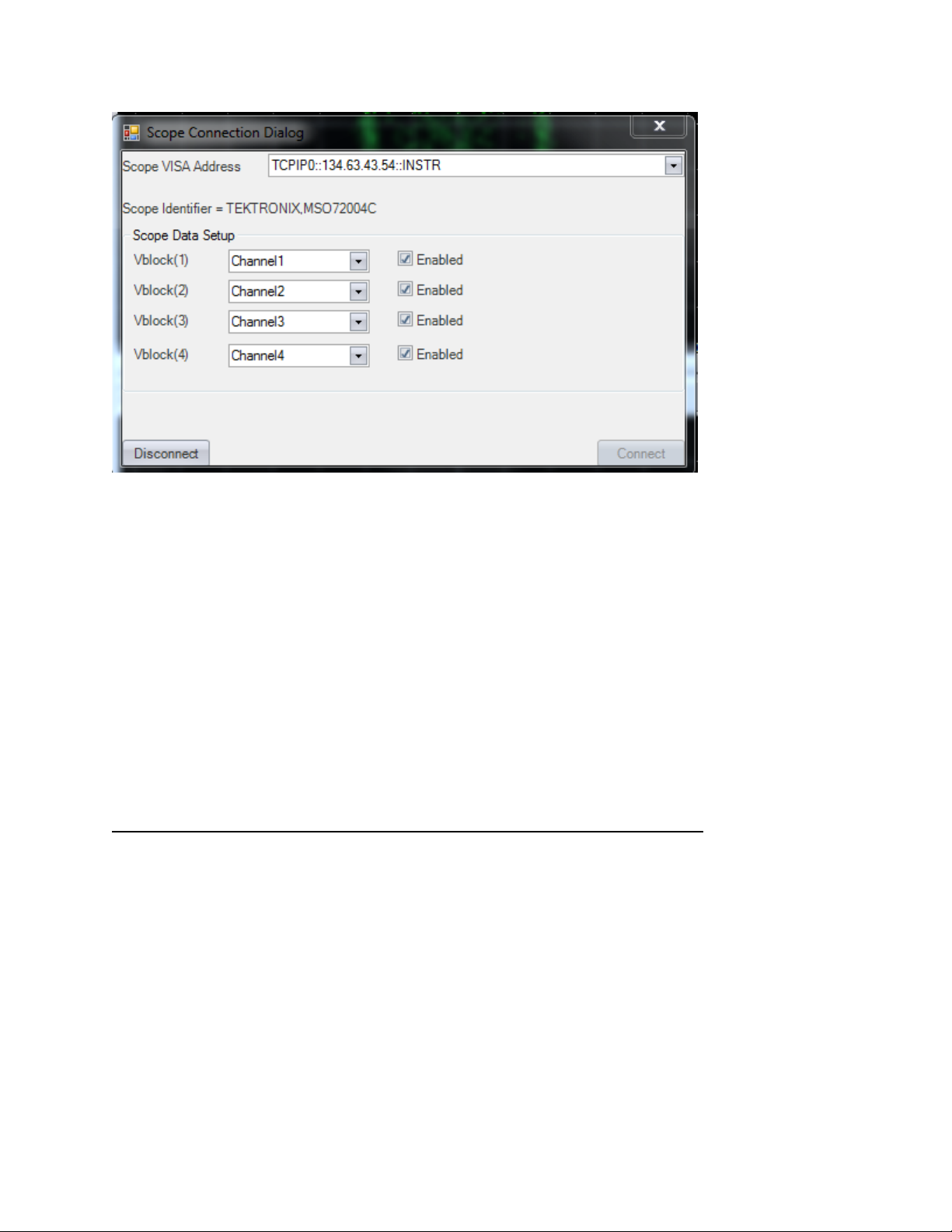
After clicking Connect, the drop down boxes will be populated for channel configuration.
Choose the oscilloscope channel name which corresponds to each receiver output and Matlab
variable name. These are:
Vblock(1) – X-polarization, In-Phase
Vblock(2) – X-polarization, Quadrature
Vblock(3) – Y-polarization, In-Phase
Vblock(4) – Y-polarization, Quadrature
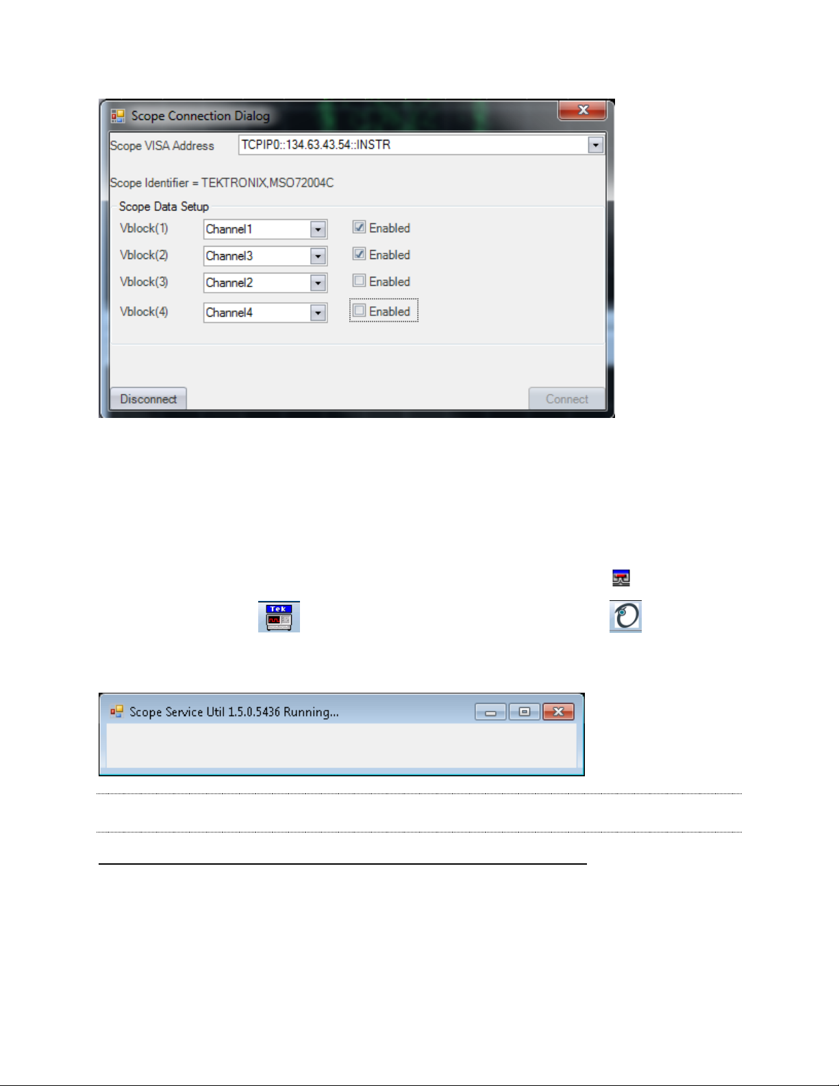
In the case below we disable two channels and set the other two to Channel 1 and Channel 3 since
these can be active channels in 100Gs/s mode. The disabled channels must still have some sort of
valid drop-down box choice. Do not leave the choice blank.
It is important to have the oscilloscope in single-acquisition mode (not Run mode). If you put the
oscilloscope into Run mode to make some adjustment, please remember to press Single on the
oscilloscope prior to connecting from the OUI.
Tektronix OM4006/OM4106 Coherent Lightwave Signal Analyzer User Guide V1.5.1 10/24 ©2012 Page 25 of 148
Page 29
3.2.3.2 Non-VISA Scope Service Connections
As mentioned above, the other choice for connecting to the oscilloscope and collecting data is the
Scope Service Utility. The Scope Service Utility is a program that runs on each oscilloscope to be
connected to the OUI.
Once the Utility is installed on the oscilloscope, please start the “Socket Server” and the
Oscilloscope Application before starting the Utility using the desktop icon .
The Scope Service has a small User Interface shown below.
Note: The Scope Service Utility runs on the target oscilloscope. Be sure to install the proper
version for either real-time or equivalent-time (ET) oscilloscopes. See installation guide.
It is best to have the oscilloscope in single-acquisition mode (not Run mode). The Scope Service
takes data directly from the oscilloscope memory and serves it up over a WCF interface to the OUI.
Tektronix OM4006/OM4106 Coherent Lightwave Signal Analyzer User Guide V1.5.1 10/24 ©2012 Page 26 of 148
Page 30
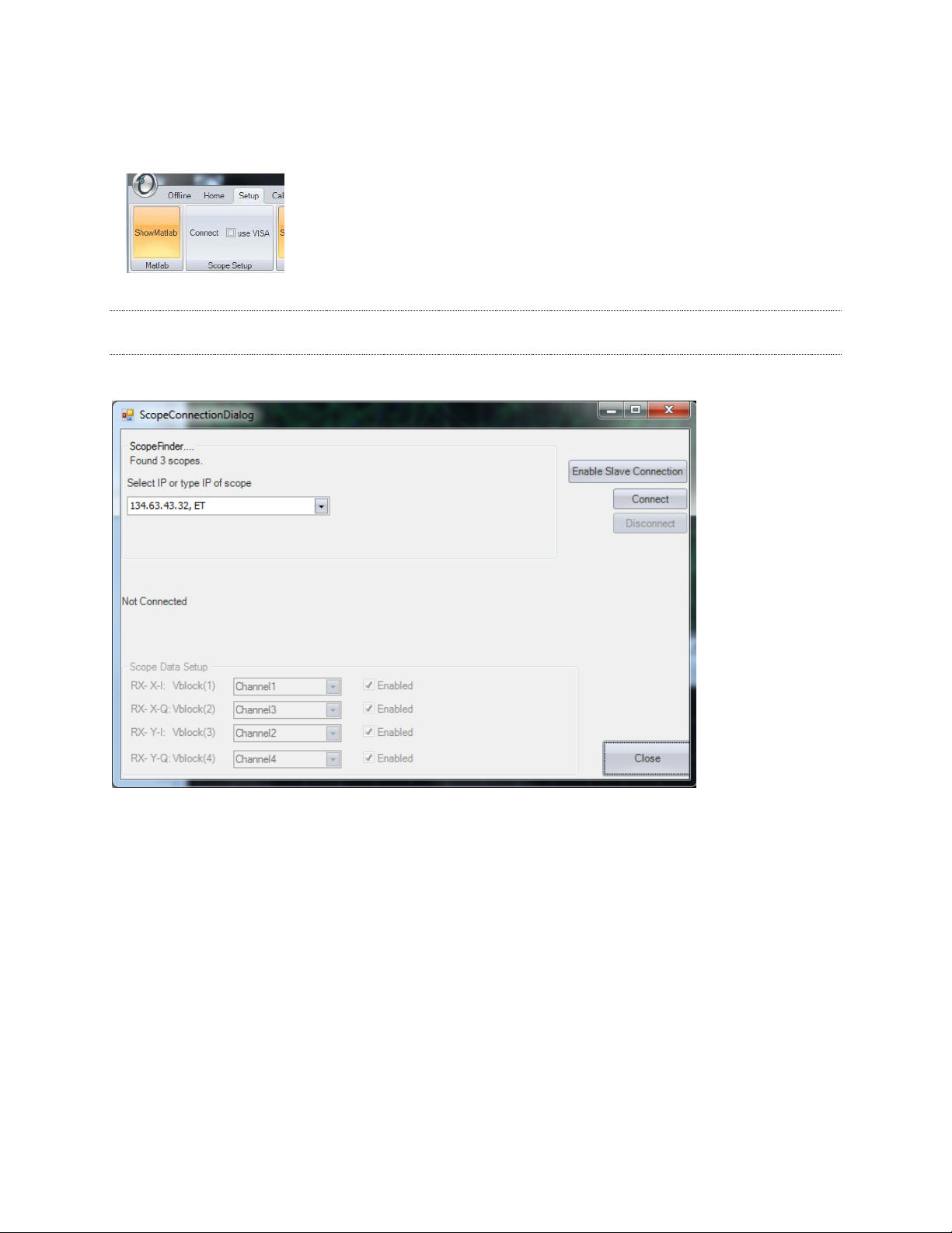
When connecting from the OUI, you will see a check box for VISA. Do not check the box unless you
require a VISA connection.
Note: Clicking Connect on the OUI Setup Tab brings up the Scope Connection Dialog box for
connecting to the Scope Service Utility
The green bar at the top indicates that the software is searching for oscilloscopes on the same
subnet that are running the Scope Service Utility. As they are found they are added to the dropdown menu. If the OUI Scope Connection Dialog box reports 0 Scopes Found, you will have to type
in the IP address manually. This happens when connecting over a VPN or when network policies
prevent the IP broadcast. When typing the address in manually, do not include “, ET” or “, RT” on the
end. Click connect.
After connection, map the channels to the physical receiver channels and corresponding Matlab
variables as shown. This means that data from the selected channel will be moved into the
indicated Vblock variable. Vblock(1) is X-Inphase, Vblock(2) is X-Quadrature, Vblock(3) is YInphase, Vblock(4) is Y-Quadrature. The mapping you choose will depend on the cable connections
made to the receiver.
Tektronix OM4006/OM4106 Coherent Lightwave Signal Analyzer User Guide V1.5.1 10/24 ©2012 Page 27 of 148
Page 31

Once connected and configured, close the connect dialog box. The OUI is ready to use.
3.2.3.3 Two-Oscilloscope Configuration – See Appendix A
OUI Version 1.5 supports a new configuration where two C- or D-model 70000-Series oscilloscopes
are both connected to an OM4000.
3.2.4 Calibration and Adjustment
The receiver requires four types of calibration:
1) DC calibration (to compensate for any offsets in the photodiode outputs)
2) Delay adjustment (channel to channel skew in the scope connections)
3) Hybrid calibration (correction for cross-talk and phase error in the hybrid)
4) Laser linewidth factor (choosing the correct filter for phase recovery)
5) Receiver equalization
3.2.4.1 DC calibration
Although the OM4000 Series units use balanced detection, there is usually some small offset
voltage present at the signal outputs. This offset voltage depends on the total optical power
input to the system and so can change. The offset is small enough that only large changes to
the reference or optical input power substantially affect the computation. “DC calibration”
Tektronix OM4006/OM4106 Coherent Lightwave Signal Analyzer User Guide V1.5.1 10/24 ©2012 Page 28 of 148
Page 32

determines the DC levels in the receiver’s photodiodes, and subtracts this off within the
analysis. This can be done as often as needed or desired. If there is uncompensated dc offset in
the system, this will be evident by a smearing out of the constellation point groups. If the offset
is large enough, the point groups will begin to look like donuts. Perform a dc calibration
whenever there is any question.
3.2.4.2 Delay adjustment
Note: Initial delay adjustment should be done by trained personnel. This section is provided for
experienced users. Delay adjustment should be done during installation and should not
require attention unless the scope is removed and/or reconnected.
Delay adjustment among the four electrical channels of the oscilloscope is done through the
Channel Delay Calibration section of the Calibrate ribbon.
Access to the delay sliders is done via the checkbox shown below. Once this is accomplished
for a specific oscilloscope installation, it should not need further attention, and should be left
untouched. If the receiver/oscilloscope interface is altered (e.g. with the installation of new
cables or shifting of the instrument), delay calibration may need to be performed.
Use the Calibration ribbon to adjust the skews to get the best possible eye diagram and
constellation diagram. Improper skew will cause horizontal eye closure and filling in of the
constellation diagram. If the I and Q channels have unequal delay, there will be a phase offset
proportional to the difference frequency between the reference and signal laser oscillation
frequencies. This phase offset will turn a straight line on the phase diagram into a circle or a
portion of a circle. So, for verification, it is best to use a known Mach-Zehnder modulator to
generate a BPSK optical input. As the input signal polarization is adjusted, the phase diagram
should always be a straight line.
Tektronix OM4006/OM4106 Coherent Lightwave Signal Analyzer User Guide V1.5.1 10/24 ©2012 Page 29 of 148
Page 33

ChDelay(2) off by 4 ps causes curvature on constellation and
signal on Q-Eye for 28Gbps BPSK
The ChDelay variable is defined as follows:
ChDelay(1): delay between channels 1 and 1 which is zero.
ChDelay(2): delay between channels 1 and 2
ChDelay(3): delay between channels 1 and 3
ChDelay(4): delay between channels 1 and 4
Automatic ChDelay Calculation
When setting up for the first time or whenever the channel delays are completely unknown, it is
best to use the utility CalChDelay as shown in the figure below. To use this utility, take the
following steps:
1) Complete the initial setup outlined in Section 3.1
2) Launch the Laser Receiver Control Panel and Connect to the OM4000 Series receiver
as outlined in Section 6 and use the drop-down menu to choose the laser to be the
reference.
3) Connect a high-baud rate BPSK signal to the Input of the OM4000 Series receiver
4) Tune the reference laser to the same WDM channel as the BPSK signal. Use the
oscilloscope controls to verify that the BPSK source is on and at proper level. It does not
Tektronix OM4006/OM4106 Coherent Lightwave Signal Analyzer User Guide V1.5.1 10/24 ©2012 Page 30 of 148
Page 34

have to be perfectly biased. Adjust the vertical gain on the oscilloscope so that the signal
is filling up at least 50% of the oscilloscope screen. Adjust the signal polarization as
needed to get good signal level on all four oscilloscope inputs.
5) Launch the OUI4006 software and connect to the oscilloscope using the Setup tab.
Ensure that the proper LO Frequency is displayed on the Setup tab as well. On the
display tab select Single-pol BPSK and also select 1 Pol BPSK on the Analysis
Parameters tab. Enter the Clock Frequency of the BPSK signal.
6) Enter the CalChDelay function in the Engine Window as shown below.
7) Click Single to take an acquisition; be sure no errors are reported in the Matlab Engine
Response.
8) Use the sliders in the Calibrate tab to set the displayed ChDelay for future use (only the
last 3 numbers are set since the first is always zero.
Manual ChDelay Determination:
Once you have used the sliders to set the delays at least close to their actual values, you can
use the shape of the phase-diagram curves to fine tune as described here. It is best to do this
one polarization at a time using the following steps:
1) Delete everything from the Matlab Engine Window except for CoreProcessing
2) Perform a DC calibration as outlined above in Section 3.2.3.2.1.
3) Adjust the input polarization so the signal is mostly on oscilloscope channels 1 and 2.
This can be done mathematically by putting the following statements before
CoreProcessing:
Vblock(3).Values = Vblock(3).Values*0.001;
Vblock(4).Values = Vblock(4).Values*0.001;
4) Now only the top slider will make any difference. Click Run to get a repeating
constellation and eye-diagram update. Click the + and – to make 0.1-ps adjustments to
Tektronix OM4006/OM4106 Coherent Lightwave Signal Analyzer User Guide V1.5.1 10/24 ©2012 Page 31 of 148
Page 35

the top slider until the BPSK constellation as perfectly straight lines connecting the two
groups of constellation points.
5) Displaying the X-Q eye will show the signal going into the “wrong” quadrature. When the
delay is set properly the signal shown should only be noise.
6) Now shut down channels 1 and 2 by again moving the polarization state of the signal or
by zeroing it be deleting the lines from item 3 and replacing them with:
Vblock(1).Values = Vblock(1).Values*0.001;
Vblock(2).Values = Vblock(2).Values*0.001;
7) Now only the difference between the bottom slider will matter.
8) Move the last slider using the + and – buttons to get 0.1-ps changes until the
constellation looks as it did with channels 1 and 2. Once again use the X-Q eye as a
measure of residual error as well as constellation quality.
9) Once this is done get equal signal on both polarizations by deleting everything from the
Engine Command Window except for CoreProcessing and adjusting the input
polarization as needed.
10) The last step is to set the middle slide to achieve minimum signal in the Y-polarization.
Since the input is a single-pol signal at this point, nothing should be in the Y constellation
or eyes except for noise.
11) Display the Y-I or Y-Q eye diagrams and Y-Constellation to see the signal going into the
wrong polarization. This should just be noise when the middle slider is set properly.
12) The delay calibration is done if there is only noise in eye plots except the X-I and only
noise in the Y-constellation.
13) Click the check box to hide the sliders to avoid accidental change
14) Save the Matlab workspace as Delay.mat for later recovery of the delay data if needed.
The delays are now stored in the ChDelay variable.
Tektronix OM4006/OM4106 Coherent Lightwave Signal Analyzer User Guide V1.5.1 10/24 ©2012 Page 32 of 148
Page 36
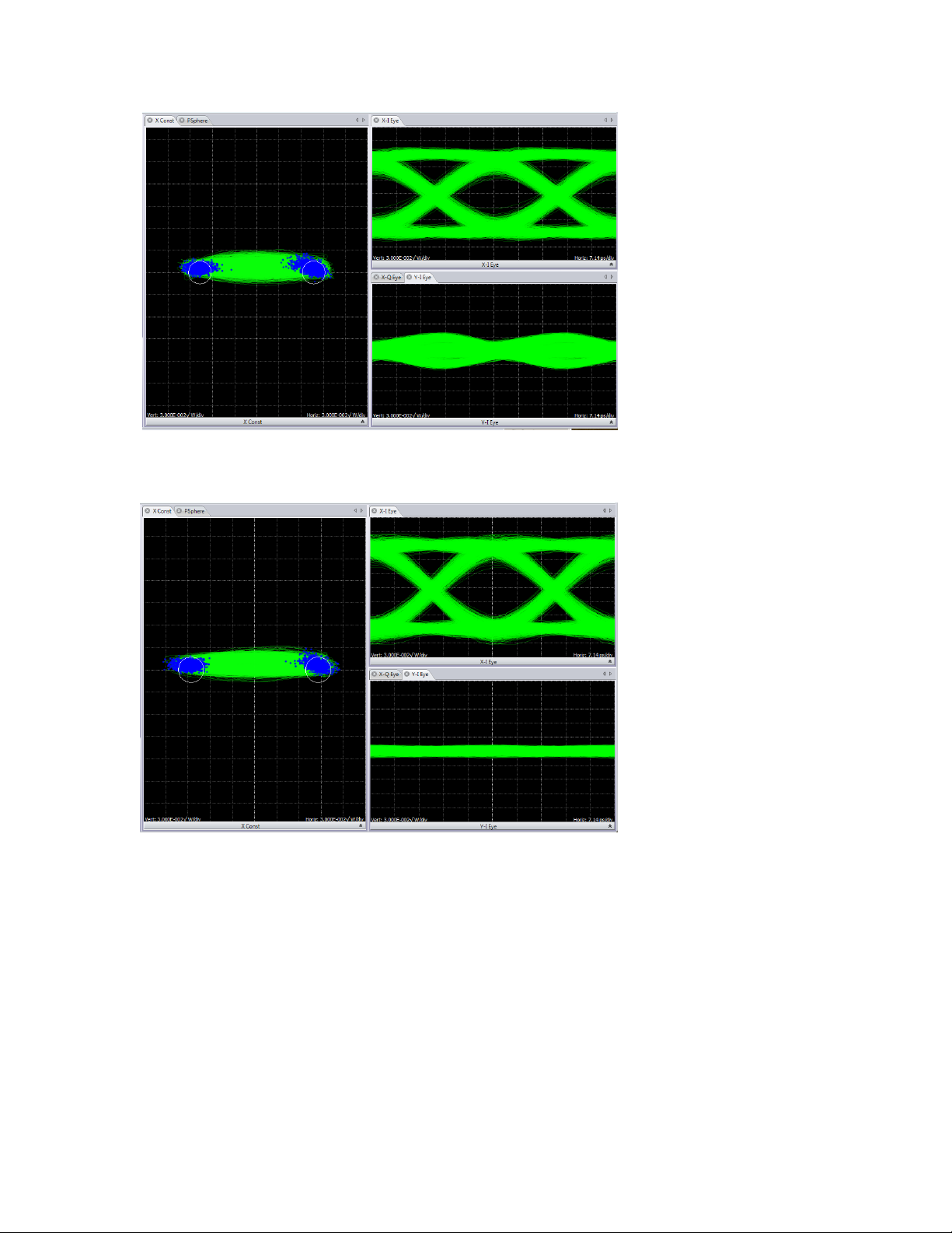
When adjusting the middle slider, watch the Y-Eye to minimize the
signal in the Y-polarization
Final Channel Delay values provide only noise in Y polarization
Tektronix OM4006/OM4106 Coherent Lightwave Signal Analyzer User Guide V1.5.1 10/24 ©2012 Page 33 of 148
Page 37
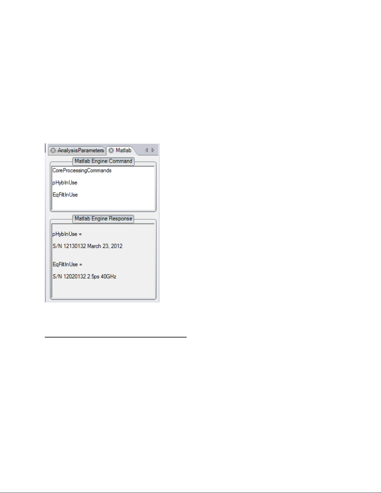
3.2.4.3 Hybrid calibration
This is a factory calibration. Imperfections in the OM4000 Series receiver are corrected using a
factory-supplied calibration table. Check the Setup tab for a green indicator to be sure the OUI is
successfully retrieving the Reference laser (Local Oscillator) frequency and power which are needed
to choose the correction factors from the calibration table. The table is the pHybCalib.mat file in the
ExecFiles directory. You can verify you have a valid pHybCalib file by connecting to an oscilloscope,
typing pHybInUse in the Matlab Engine Window, and clicking Single. Similarly, EqFiltInUse shows
the equalization filter in use (if any).
The info statement contains the serial number, date of calibration, and other notes about the
calibration. If the serial number is correct then you have the proper file.
Calibration Check and Quick-Cal Procedure
The following procedure can be used to verify and correct the calibration at a single wavelength
using a minimum of external hardware. This procedure assumes that “Laser 1” and Laser 2” can be
tuned to the same wavelength. It is easiest if you have a polarization controller before the signal
input, but the instructions are written assuming you are moving the fiber around to change the input
polarization.
1) Equipment set up for optical hybrid calibration verification:
a. System should be de-skewed following the procedure above.
b. Connect the Reference as usual from Laser 2 to the Reference input with short PM/APC
jumper.
c. Use a standard SM/APC (not PM) fiber to connect the Laser 1 to the Signal input. Use
the LRCP to set the Signal 1 power level to about 10dBm to start.
Tektronix OM4006/OM4106 Coherent Lightwave Signal Analyzer User Guide V1.5.1 10/24 ©2012 Page 34 of 148
Page 38
d. Use the LRCP to turn on both lasers and tune them to the same channel where you will
be working. Set the Laser 1 power to get about 100mV pp.
e. Use the LRCP to tune Laser 1 off grid by 100 to 500MHz
f. Click Run on the oscilloscope to get a rapidly updating display. You should see 100 to
500 MHz sine waves.
g. Move the SM fiber around until you get most signal on channels 1 and 2 (at least 3:1 ra-
tio between Channels 1 and 3. This is most easily done with a polarization controller).
h. Tape the fiber down so that you continue to get most signal on Channels 1 and 2.
i. Click Single on the oscilloscope.
2) Procedure to Inspect and Correct the X-polarization Calibration:
a. Use the Optametra OUI to connect to the scope. Record length of ~20,000 points rec-
ommended in single block (BlockSize > 20,000).
b. Display the Matlab Engine Window, the X-Constellation Window and the Y-Constellation
Window. Close other windows.
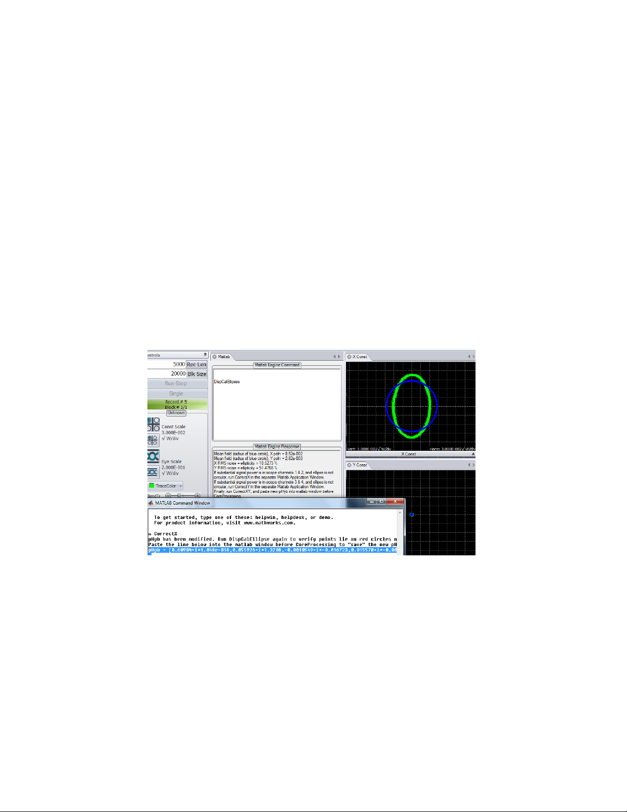
c. Put DispCalEllipses in the Matlab Engine Window of the OUI. Delete everything else in
the Matlab Engine Window.
d. Click Run on the Optametra OUI
e. Observe that the ellipses are displayed on the Constellation plots. Right now only the X-
constellation has signal. The green trace should line up with the blue circle in the Xconstellation plot.
f. If the green trace in X-Constellation is elliptical:
i. Click Stop
ii. Type CorrectX in the separate Matlab Engine Window
iii. Copy and paste the resulting pHyb statement before DispCalEllipses in the
Matlab Engine Window in the OUI as shown below.
g. Click Run. The green trace should now be circular.
Tektronix OM4006/OM4106 Coherent Lightwave Signal Analyzer User Guide V1.5.1 10/24 ©2012 Page 35 of 148
Page 39

3) Procedure to Inspect and Correct the Y-polarization Calibration
a. Move the input fiber to get most of the signal on Channels 3 and 4. Tape it down.
b. Click Single on the Oscilloscope. Click Run on the OUI
c. Observe that the ellipses are displayed on the Constellation plots. Right now only the Y-
constellation has signal. The green trace should line up with the blue circle in the Yconstellation plot.
d. If the green trace in Y-Constellation is elliptical:
i. Click Stop
ii. Type CorrectY in the separate Matlab Engine Window
iii. Copy and paste the resulting pHyb statement before DispCalEllipses, replacing
any other pHyb statement.
e. Click Run. The green trace should now be circular.
Tektronix OM4006/OM4106 Coherent Lightwave Signal Analyzer User Guide V1.5.1 10/24 ©2012 Page 36 of 148
Page 40

4) Procedure to Correct the relative X-Y gain.
a. You must complete all of the above steps first including CorrectX and CorrectY.
b. Type CorrectXY in the separate Matlab Engine Window
c. Copy and paste the resulting pHyb statement before DispCalEllipses, replacing any other
pHyb statement.
d. Move the input fiber until there is signal on all four channels
e. Click Run. The green trace should now be circular in both Constellations.
5) The pHyb statement in step 5 is the final output that is corrected for Ch1-2 gain and phase, Ch3-
4 gain and phase, and Ch1-3 gain.
Tektronix OM4006/OM4106 Coherent Lightwave Signal Analyzer User Guide V1.5.1 10/24 ©2012 Page 37 of 148
Page 41

6) Replace the DispCalEllipses statement with CoreProcessing for normal operation. Keep the
Scope Sampling Rate
Reference Magnitude Response
Reference Phase
≤ 2x the bandwidth of the
OM4000 Series unit (BW)
Flat
Linear
> 2x the bandwidth of the
OM4000 Series unit (BW)
4th order digital (bilinear) Bessel
filter with 3dB cutoff at BW + 2GHz
Linear
pHyb statement as it is correcting the calibration.
3.2.4.4 Absolute Power Calibration
As of version 1.2.0, the OUI has the ability to provide signal data plotted on an absolute scale
independent of the LO signal strength. This requires absolute scaling of the pHybCalib.mat file which
was not available on all earlier versions. Check the absolute scale by connecting a CW signal of
known power (no modulation) with sufficient power to fill most of the oscilloscope display. Be sure
the OUI and LRCP are connected by checking for the green square on the SetUp Tab. Do a DC
calibration. The OUI should display one group of symbols in the X constellation. The distance from
the center of that group to the origin is the signal strength in root-Watts. Square this value and
compare to the known value in Watts. To use the built in Magnitude measurement, choose BPSK
signal type and a clock frequency equal to twice the offset between the signal and LO frequencies.
This will display two clusters of points and the Magnitude measurement will provide the average
signal strength. The power calibration should be accurate to 15%.
3.2.4.5 Laser linewidth factor
See discussion in Section 5.2 on modifying the default value of “Alpha.”
3.2.4.6 Receiver Equalization
Receiver Equalization is a factory calibration. Digital equalization is applied to the four channels
of the OM4000 Series receiver to account for the non-ideal frequency dependent response
introduced by the coherent optical receiver and the receiver radio frequency front end.
Depending on the sampling rate of the oscilloscope and the bandwidth of the OM4000 Series,
digital equalization is applied so that the combined effect of the receiver and the digital
equalization filter meet a specified reference response:
Equalization is specific to the sampling rate of the oscilloscope. As an example, if the bandwidth
of the OM4000 Series is 30 GHz and the sampling rate of the oscilloscope is 80 GSPS, the
Tektronix OM4006/OM4106 Coherent Lightwave Signal Analyzer User Guide V1.5.1 10/24 ©2012 Page 38 of 148
Page 42

combined effect of the OM4000 Series receiver front end response and the digital equalization
0 0.5 1 1.5 2 2.5 3 3.5 4
x 10
10
-20
-15
-10
-5
0
Frequency
Magnitude response (dB)
Reference filter responose
filter will be that of a 4th order digital Bessel filter with 3dB cutoff at 32GHz (see below).
The digital filter is applied directly to the MATLAB workspace variables Vblock(1).Values through
Vblock(4).Values using a 100 tap FIR filter.
For more information, or for equalization support of a different scope sampling rate, contact
customer support.
3.2.5 Moving and Docking Windows
The OUI is designed to allow you maximum control of the graphical presentation. There are
three types of displays in the OUI: ribbons, fly-out panels, and windows. The main ribbon,
shown below, is normally displayed making the various tabs always available. To get more room
for graphics, you can hide the ribbon by double clicking in the tab area. Bring it back by double
clicking again on one of the tabs.
Flyout panels are used for information that is needed less often. Mousing over the Measurement
tab on an eye-diagram for example will bring up the panel below. Clicking on the push pin will
cause the panel to stay after you mouse away.
Tektronix OM4006/OM4106 Coherent Lightwave Signal Analyzer User Guide V1.5.1 10/24 ©2012 Page 39 of 148
Page 43

The graphics windows can be docked or free floating. To move a graphics window, click and
hold over the tab then drag. As you drag the window, different docking targets will appear as
shown below. Moving the pointer to the center of the target will cause the window being
dragged to be displayed on top of the existing window. Dragging it to one of the four squares
surrounding the center of the docking target will split the window so that both the new and old
windows are visible. You may also drag the window to another monitor or leave it free floating in
front of the OUI main window.
Tektronix OM4006/OM4106 Coherent Lightwave Signal Analyzer User Guide V1.5.1 10/24 ©2012 Page 40 of 148
Page 44

3.2.6 Laser / Receiver Control Panel (see Section 6 for first use)
3
Channel setting within the ITLA grid gives the corresponding frequency (in THz) and wavelength
(in nm). Power is set within the range allowed by the laser. It is best to set the Signal and
Reference lasers to within 1 GHz of each other. This is simple if using the internal OM4000
Series lasers: just type in the same channel number for each. If using an external transmitter
laser, you can type in its wavelength and the controller will choose the nearest channel. If this is
not close enough, try choosing a finer WDM grid or use the fine tuning feature. If available3, fine
tuning of the laser is done with the Fine Tune slider bar, and typically works over a range of +/10 GHz from the center frequency of the channel selected. Certain laser models have a cavity
lock feature that increases their frequency accuracy at the expense of dithering the frequency;
this feature can be toggled with the Cavity Lock button. Cavity Lock is necessary to tune the
laser, but can be unchecked to suppress the dither.
Once the Channel and Power for each laser is set, turn on laser emission for each laser by
clicking on its Laser Emission button; the emission status is indicated both by the orange
background of the button and by the corresponding green LED on the OM4000 Series front
panel.
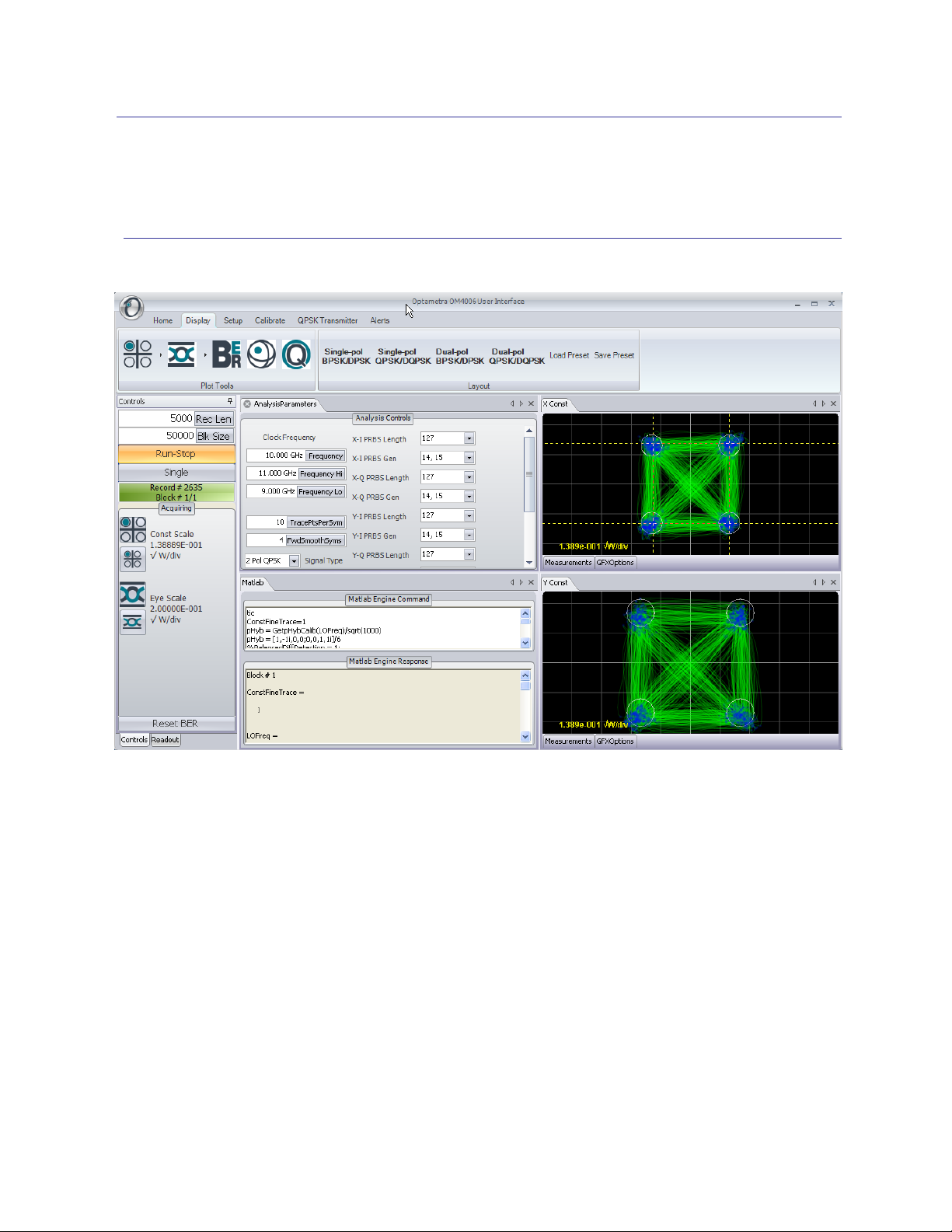
3.2.7 Matlab
When it is launched, the OUI in turn launches the default Matlab installation.
The default working directory is the installation directory. Use the cd command to change to
another directory if desired. Any files saved will go to the working directory. Once the OUI is
running, the Matlab workspace is populated with the variables and functions used in coherent
signal processing:
For example, the standard OM3x05 ships with Emcore lasers, which can be fine tuned.
Tektronix OM4006/OM4106 Coherent Lightwave Signal Analyzer User Guide V1.5.1 10/24 ©2012 Page 41 of 148
Page 45

3.2.8 Licensing
The software bundled with the OM4000 Series is licensed per the agreement in the Appendix.
Copy protection is enabled via HASP key, which must be present in permanent installations.
Tektronix OM4006/OM4106 Coherent Lightwave Signal Analyzer User Guide V1.5.1 10/24 ©2012 Page 42 of 148
Page 46

4 Making Measurements
4.1 Setting Up Your Measurement
Since the Coherent Lightwave Signal Analyzer is a reconfigurable (complex, dual-polarized)
reference receiver, it requires a modulated signal on the input fiber. Depending on the options
configured in the receiver, this modulation can be single- or dual-polarized, with several formats
available, including OOK (on-off keying), BPSK (binary phase-shift keying), and QPSK
(quadrature phase-shift keying), either coherent or differential.
The Coherent Lightwave Signal Analyzer includes two (C- or L-band) network-tunable sources;
you can use these or your own lasers for signal and reference inputs. Furthermore, each
polarization can be independently driven by a distinct source, though all sources must be tuned
to the same (ITLA) channel, or at least to the same wavelength. While no phase locking of the
sources is necessary, the beatnote between any signal laser and the reference should be at a
low enough frequency that the bandwidth of the real-time oscilloscope can accommodate the
modulation bandwidth plus the beatnote frequency.
Prior to testing a modulated source, ensure that there is no modulation of the lasers (i.e. that
your data source [pattern generator] is not enabled). With both lasers emitting and tuned to the
same channel, use the fine-tune feature of the Laser/Receiver Control Panel to obtain a 100500 MHz beat note on the oscilloscope. Then enable modulation, e.g. by activating your data
source or pattern generator.
4.2 Engine file
You can configure Matlab to perform a wide range of mathematical operations on the raw or
processed data using the Engine window. Normally the only call is to
CoreProcessingCommands, the set of routines performing phase and clock recovery.
Note: Accessing the Matlab Command Window and typing who will result in a full list of varia-
bles.
Tektronix OM4006/OM4106 Coherent Lightwave Signal Analyzer User Guide V1.5.1 10/24 ©2012 Page 43 of 148
Page 47

Note that CoreProcessingCommands will provide either ET or RT processing depending on what
mode the OUI is in. To ensure you only get ET processing you can use CoreProcessingET in the
window instead of CoreProcessingCommands. Similarly you can use CoreProcessing in the
Engine Window if you want to be sure you only get real-time processed data.
As with all other settings, the last engine file used is recalled; you can locate or create another
appropriate engine file and paste it into the OUI Matlab window. Subsequent chapters explain in
detail the operations of Core Processing.
In addition to any valid Matlab operations you may wish to use, there are some special variables that
can be set or read from this window to control processing for a few special cases:
EqFiltInUse – a string which contains the properties of the equalization filter in use
pHybInUse – a string which contains the properties of the optical calibration in use
DebugSave – logical variable that controls saving of detailed .mat files for analysis
DebugSave = 1 in the Matlab Engine Command window results in two files saved per block
plus one final save.
DebugSave = 0 or empty suppresses .mat file saves.
4.3 Performing measurements
Click on Single, and observe that the oscilloscope takes a burst of data; this
confirms the connection. Using a short record length (e.g. 2000 points) to speed up the display,
click on Run-Stop to show continuously-updated measurements.
Tektronix OM4006/OM4106 Coherent Lightwave Signal Analyzer User Guide V1.5.1 10/24 ©2012 Page 44 of 148
Page 48

Using the Home tab, set up the plots you want, either using the stored Layout button or by
clicking on the particular display format icon in the Plot Tools bar.
Display format icons (from left): Constellation, Eye, Bit Error Rate
(BER), Poincare Sphere. Presets are shown at right.
Displays can be rearranged within the UI window or dragged and positioned randomly on the
Windows Desktop. Clicking and dragging a window using its title tab brings up a positioning
guide. Hold down the left mouse button to position the window onto the positioning guide, then
release to organize the plots.
Constellation and Eye plots can be rescaled by clicking on the relevant scaling icons in the
Controls tab of the left panel of the UI. The scale in √W/div is indicated.
Options for each plot are accessed by Right-Clicking on the plot. Trace and symbol contrast can
be set globally using the sliders on the left bar of the OUI. Set trace and symbol properties for a
particular plot using the Right-Click on the plot.
Tektronix OM4006/OM4106 Coherent Lightwave Signal Analyzer User Guide V1.5.1 10/24 ©2012 Page 45 of 148
Page 49
5 Using the OUI
5.1 OUI Overview
The panel on the left side titled “Controls” is typically pinned so that it is always present to allow
control of the acquisition and plot scale. The first entry, Rec Len, determines the oscilloscope
record length for the next acquisition. The record length in turn determines the horizontal time
scale given a fixed sampling rate. Since different oscilloscopes allow different record lengths,
the OUI will replace your entry with the closest available larger record length after you click
Single or Run-Stop to start the acquisition.
The second entry in the Control panel is Blk Size. Block Size is the number of points that are
processed at one time. For record lengths up to 10,000 or even 50,000 points, it makes sense
to process everything at once. This will happen if Blk Size is greater than or equal to Rec Len.
However, for record sizes above 50,000, there can be a delay of many seconds waiting for
processing. In this case, breaking the processing up into blocks gives you more frequent screen
Tektronix OM4006/OM4106 Coherent Lightwave Signal Analyzer User Guide V1.5.1 10/24 ©2012 Page 46 of 148
Page 50

updates and a progress bar so know what is happening while you wait. This is accomplished by
Rec Len
Blk Size
Behavior
< 1,000,000
≥ Rec Len
All data processed in one block. Aggregated variables
such as constellation and eye diagrams available for
plotting.
< 1,000,000
< Rec Len
Data broken up into blocks for processing. Aggregated
variables such as constellation and eye diagrams
available for plotting after each block has completed.
> 1,000,000
< 1,000,000
Data broken up into blocks for processing. Only BER and
other summary measurements are aggregated block to
block. Raw data and time series variables are erased
when next block is processed. Need to save workspace
of intermediate blocks of interest for later viewing.
Run/Stop mode is disabled.
Any
= 1,000,000
The maximum allowable entry in the Blk Size field is
1,000,000.
simply choosing Blk Size < Rec Len. Block Processing is further explained in Section 10.5.
Block Processing is most important when the size of the record is so large that it begins to tax
the memory limits of the computer. This can begin to happen at 200,000 points but is more likely
a problem at 1,000,000 points and above for XP machines with maximum RAM. For these
record sizes between 1,000,000 and the oscilloscope memory limit (usually many tens or
hundreds of megapoints), it is essential to break processing into blocks to avoid running out of
processor memory. In addition, since neither the entire waveform, nor the entire processed
variables will fit in computer memory at one time, it is necessary to make some decisions as to
what information will be retained as each block is processed. By default raw data, electric field
values, and other time series data are not aggregated over all blocks in a record greater than
1,000,000 samples. For more detail on how to manage large data sets, see Section 5.13.
Tektronix OM4006/OM4106 Coherent Lightwave Signal Analyzer User Guide V1.5.1 10/24 ©2012 Page 47 of 148
Page 51

5.2 Analysis Parameters
The Analysis Parameters window allows you to set parameters relevant to the system and its
measurements. When any parameter is clicked on (left hand column) help on that item is
displayed in the window at the bottom of the parameter table.
Signal Type: Chooses the type of signal to be
analyzed and so also the algorithms to be applied
corresponding to that type.
Pure Phase Modulation: Sets the clock recovery
for when there is no amplitude modulation.
Clock Frequency: Is the nominal frequency of
the clock recovered by CoreProcessing bounded
by a low (Low) and a high frequency (High)
provided the clock signal power is sufficient;
Assume Orthogonal Polarizations: Checking
this box forces Core Processing to assume that
the polarization multiplexing is done in such a
way that the two data signals have perfectly
orthogonal polarization. Making this assumption
speeds processing since only one polarization
must be found while the other is assumed to
orthogonal. In this case, the resulting SOPs will
be a best effort fit if the signals are not in fact
perfectly orthogonal. Unchecking the box forces
the code to search for the SOP of both data
signals.
Reset SOP Each Block: Checking this causes
the SOP to be recalculated for each Block of the
computation. By adjusting the Block Size (see
Blk Size) you can track a changing polarization.
When false, the SOP is assumed constant for the
entire Record (see Rec Len).
2nd Phase Estimate: Checking this box forces Core Processing to do a second estimate of the
laser phase after the data is recovered. This second estimate can catch cycle slips, that is, an
Tektronix OM4006/OM4106 Coherent Lightwave Signal Analyzer User Guide V1.5.1 10/24 ©2012 Page 48 of 148
Page 52

error in phase recovery that results in the entire constellation rotating by a multiple of 90
)ln(/T
degrees. Once the desired data pattern is synchronized with the incoming data stream, these
slips can be removed using the known data sequence.
Homodyne: The first step in phase estimation is to remove the residual IF frequency that is the
difference between the LO and Signal laser frequencies. The function EstimatePhase will fail if it
there is no difference frequency. This case occurs when the Signal laser is split to drive both the
modulator and the Reference Input of the receiver (ie. only one laser). Checking the Homodyne
box will prevent EstimatePhase from failing by adding an artificial frequency shift, which is
removed by EstimatePhase.
Phase estimation time constant parameter: (Alpha) After removing the optical modulation
from the measured optical field information, what remains is the instantaneous laser phase
fluctuations plus additive noise. Filtering the sample values improves the accuracy of the laser
phase estimation by averaging the additive noise. The optimum digital filter has been shown to
be of the form 1/(1+z-1) where is related to the time constant, of the filter by the relation
where T is the time between symbols. So, an when the baud rate is
10Gbaud gives a time constant, ps or a low-pass filter bandwidth of 350 MHz. The value
of also gives an indication of how many samples are needed to provide a good
implementation of the filter since the filter delay is approximately equal to the time constant.
Continuing with the above example, approximately 5 samples (~ T are needed for the filter
delay. This of course is not a problem, but an would require 1000 samples and put a
practical lower limit on the record length and block size chosen for the acquisition. As a simple
rule, the record or block size should be ≥ 10/(1-).
The selection of the optimum value of Alpha is discussed later in the CoreProcessing guide
Section 11.6 and reference [1]. This optimum value depends on the laser linewidth and level of
additive noise moving from a value near 1 when the additive noise is vastly greater than the
phase noise to a value near zero when phase noise is the only consideration (e.g. no filtering
needed). In practice, a value of 0.8 is fine for most lasers. If Alpha is too small for a given laser
there will be insufficient filtering which is evidenced by an elliptical constellation group with its
long axis pointed toward the origin (along the symbol vector). When Alpha is too large then
there is excessive filtering for the given laser linewidth. Excessive phase filtering is evidenced
by the constellation group stretching out perpendicular to the symbol vector and may also lead
to non-ideal rotation of the entire constellation.
Tektronix OM4006/OM4106 Coherent Lightwave Signal Analyzer User Guide V1.5.1 10/24 ©2012 Page 49 of 148
Page 53

As is often the case, when laser frequency wander is greater than the linewidth, very long
2/
2
2
)(
i
eH
c
Dpsnm
2
10
10
*
2
0
9
12
2
record lengths will lead to larger variance in laser phase. This means that an Alpha that worked
well with 5000 sample points might not work well with 500,000 points. Longer record lengths will
not be a problem if you choose a block size small enough that peak-to-peak frequency wander
is on the order of the laser linewidth. For the lasers supplied with the OM4000 Series receiver, a
block size of 50,000 points is a good choice. See Section 5.1 on Block Processing for further
information.
Balanced Differential Detection: Checking this box causes the differential-detection emulator
to emulate balanced instead of single-ended detetection.
Continuous Traces: Checking this box ensures that the fine traces connecting the constellation
points will be drawn. If unchecked, the traces will be suppressed for calculation speed if the
calculations are not needed for other plots such as eye diagrams.
Mask Threshold: The ratio of radius to symbol spacing used for the circular constellation
masks.
Continuous trace points per symbol: is the number of samples per symbol for the clock
retiming that is done to create the fine traces in the phase and eye diagrams.
Tributaries contribution to average: the average waveforms are based on finding the symbol
impulse response and convolving with the data pattern. This setting switches which possible
crosstalk contributions are included in the calculation of impulse response.
Number of symbols in impulse response: the number of values calculated for the impulse
response. More values should provide a more accurate average but take longer to calculate.
Show linear average eye: controls computation of the average eye. Refresh rate is faster when
disabled, but must be enabled for the linear average to be displayed in an eye diagram.
Show linear average vs. time: controls computation of the average signal vs. time. Refresh
rate is faster when disabled, but must be enabled for the linear average to be displayed in the X
v. T diagram.
Show transition average: controls computation of the transition average. Refresh rate is faster
when disabled. However, this must be checked to enable calculations based on transition
average such as risetime.
Compensate CD: Checking this box will apply a mathematical model to remove chromatic
dispersion. The mathematical model used for the inverse filter is:
; where
Tektronix OM4006/OM4106 Coherent Lightwave Signal Analyzer User Guide V1.5.1 10/24 ©2012 Page 50 of 148
Page 54
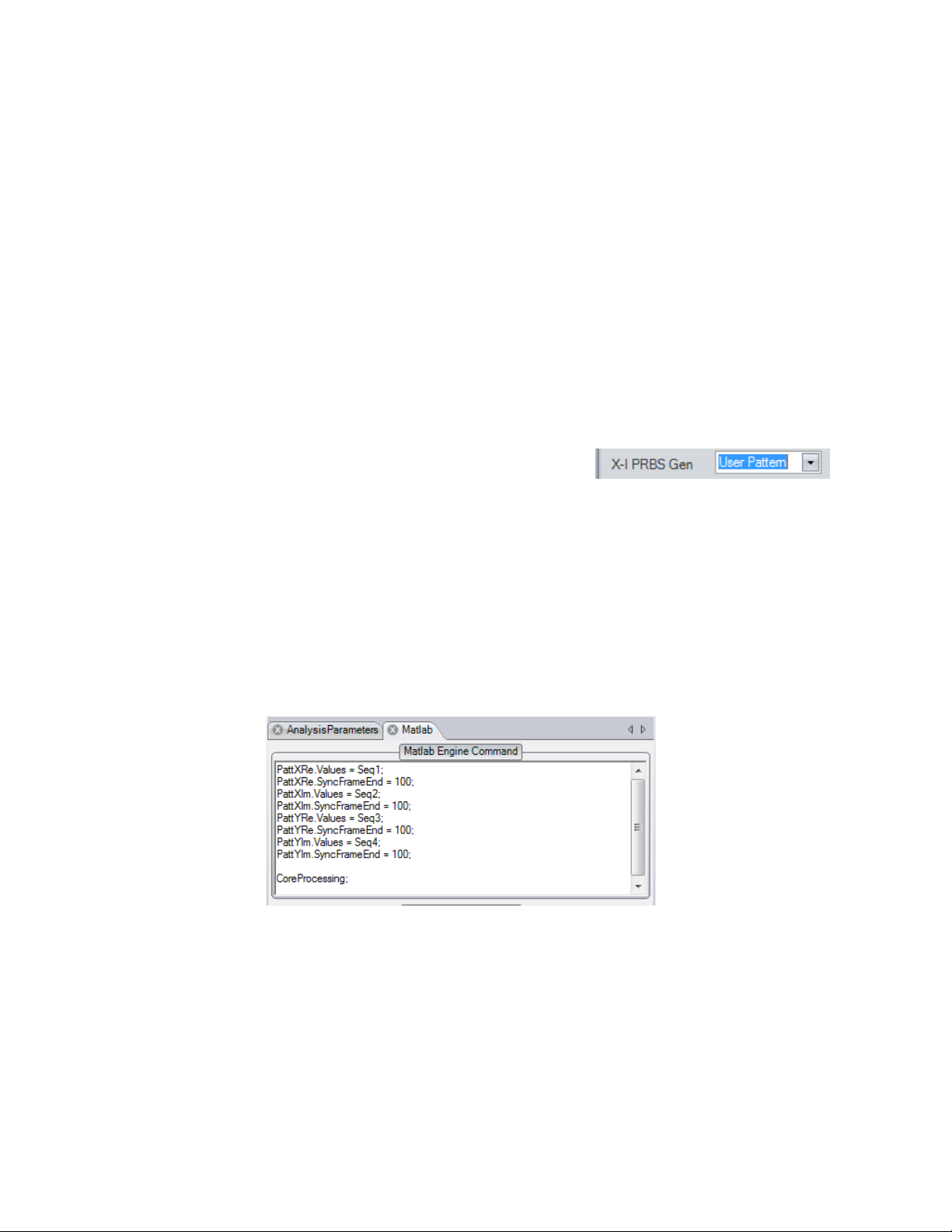
Chromatic Dispersion is the value of Dpsnm used by the CD compensation function in ps/nm.
The sign of Dpsnm should be the same as that of the dispersion compensating fiber that it
replaces. In other words, CDcomp is a dispersion compensator with dispersion, Dpsnm.
PMD: See the section on PMD measurement for a description of the controls.
Data Content: For error counting, constellation orientation, and two-stage phase
estimation, the data pattern of each tributary must be specified. Omitting the data specification
or providing incorrect information about your data pattern will not impair the constellation or eye
displays except that there will be no consistent identification of each tributary since the
identification of I and Q and X and Y is arbitrary in the case where the data is not known.
Identify your data patterns for each tributary by choosing a standard PRBS from the drop-down
menu, or by assigning the pattern variable directly. When assigning the variable directly be sure
to select user pattern from the drop-down menu first.
5.2.1 Direct assignment of pattern variables when not using a PRBS
When the transmitter is sending something other than a PRBS, even if it is just a DQPSK precode, the analyzer needs to know what data is being sent in order to calculate the BER. In this
case, it is necessary to load your pattern into MATLAB and assign it to the pattern variable. The
four lines below assign the user’s pattern variables Seq1, Seq2, Seq3, and Seq4 to the four
tributaries.
These variables must be loaded into the separate Matlab Command Window as shown below.
Tektronix OM4006/OM4106 Coherent Lightwave Signal Analyzer User Guide V1.5.1 10/24 ©2012 Page 51 of 148
Page 55

In the case shown, a previously saved .mat file is loaded and the Seq variable is created using
the PattXRe.Values content. The figure also shows the resulting size of the Seq variable as well
as the first 10 values. The pattern for each tributary may have any length, but must be a row
vector containing logical values.
Synchronizing a long pattern can take a long time. The easiest way to keep calculations fast
when using non-PRBS patterns longer than 2^15 and if using record lengths long enough to
capture at least as many bits as in the pattern, is to simply use the .SyncFrameEnd field as
shown above. Otherwise contact customer support for help in optimizing the synchronization.
5.2.2 Example capturing unknown pattern
Another way to load the pattern variable when using a pattern that is not one of the PRBS
selections is to use the CLSA to capture the pattern and store it in a variable. Here are the
steps:
1) Connect the optical signal with the desired modulation pattern to the CLSA
2) Set up the Analysis Parameters properly with the exception of the data pattern which is
not yet known
3) Choose any PRBS as the data pattern. Don’t choose “User Pattern” yet
4) No Q factor will be available since the pattern is not known, but you can optimize the
signal to achieve open eye-diagrams and low EVM so that no errors are expected
5) Set the record length long enough to capture the entire data pattern. For example, you
need 32,767 bits to capture a 2^15-1 pattern. So if this is at 28Gbaud and the scope has
a sampling rate of 50Gs/s, then you need at least 32,767*50/28 = 58,513 points in the
record. Stop acquisition after successfully displaying a good constellation with sufficient
Tektronix OM4006/OM4106 Coherent Lightwave Signal Analyzer User Guide V1.5.1 10/24 ©2012 Page 52 of 148
Page 56

record length. All the data you need is now in the MATLAB workspace. It just needs to
be put in the proper format for use in the pattern variable.
6) In the separate MATLAB Command Window, add the following commands:
a. For QPSK:
PattXReM = real(zXSymUI.Values) > 0;
PattXImM = imag(zXSymUI.Values) > 0;
b. For dual-pol QPSK add these commands:
PattYReM = real(zYSymUI.Values) > 0;
PattYImM = imag(zYSymUI.Values) > 0;
7) To get a single full pattern, delete the extra data as follows (in this case for 32,767 bits) :
a. For QPSK:
PattXReM = PattXReM(1: 32767);
PattXImM = PattXImM(1: 32767);
b. For dual-pol QPSK add these commands:
PattYReM = PattYReM(1: 32767);
PattYImM = PattYImM(1: 32767);
8) In the CLSA Matlab Engine Command Window, add the following lines prior to the
CoreProcessing statement:
a. For QPSK:
PattXRe.Values = PattXReM;
PattXIm.Values = PattXImM;
b. For dual-pol QPSK add these commands:
PattYRe.Values = PattYReM;
PattYIm.Values = PattYImM;
9) Now select User Pattern for any of the tributaries where you assigned a user pattern in
the prior step.
10) You should now be able to measure BER and Q using your new patterns.
11) To save the patterns for later use, type the following in the separate Matlab Command
Window: save(‘mypatterns.mat’,’PattXReM’, ’PattXImM’, ’PattYReM’, ’PattYImM’)
Tektronix OM4006/OM4106 Coherent Lightwave Signal Analyzer User Guide V1.5.1 10/24 ©2012 Page 53 of 148
Page 57
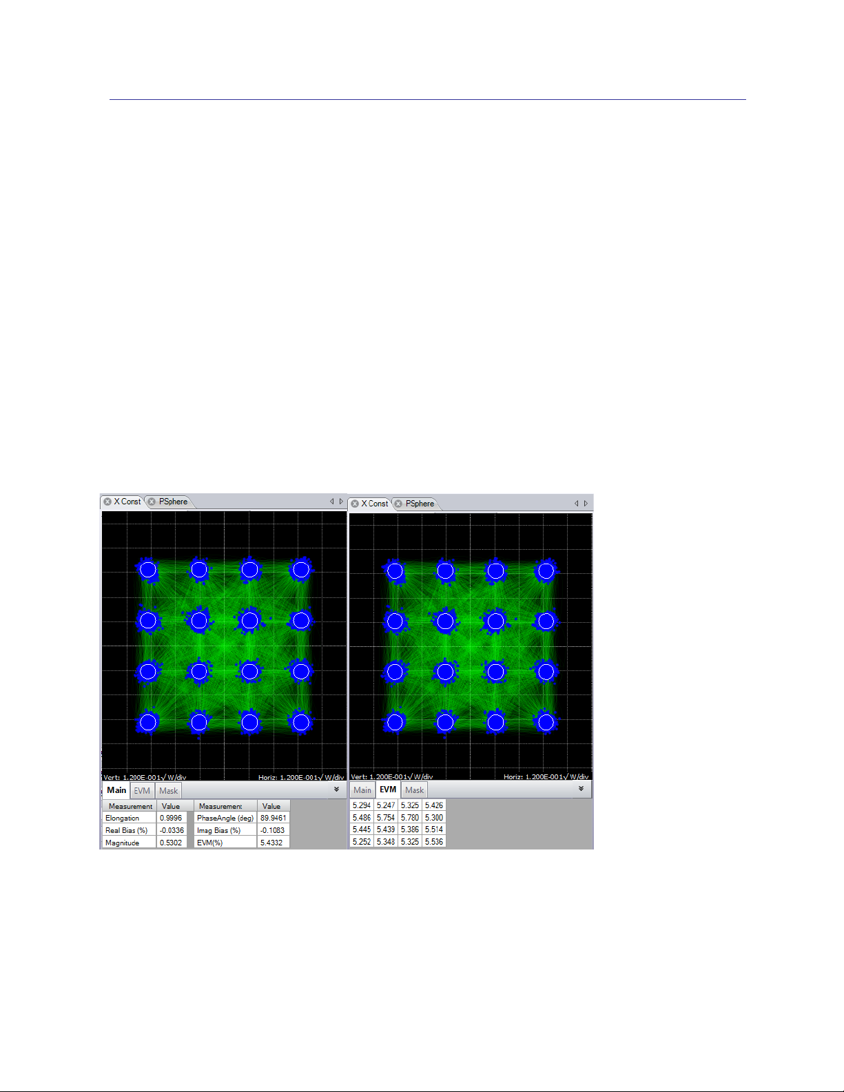
5.3 Constellation Diagrams
Once the laser phase and frequency fluctuations are removed, the resulting electric field can be
plotted in the complex plane. When only the values at the symbol centers are plotted, this is
called a Constellation Diagram. When continuous traces are also shown in the complex plane,
this is often called a Phase Diagram. Since the continuous traces can be turned on or off, we
refer to both as the Constellation Diagram. The scatter of the symbol points indicates how close
the modulation is to ideal. The symbol points spread out due to additive noise, transmitter eye
closure, or fiber impairments. The scatter can be measured by symbol standard deviation, error
vector magnitude, or mask violations.
5.3.1 Measurements
Measurements made on constellation diagrams are the most comprehensive in the OUI.
Numerical measurements are available on the “fly-out” panel associated with each graphic
window. The measurements available for constellations are described below.
Elongation: The mean inter-symbol spacing of the quadrature signals divided by the
mean inter-symbol spacing of the in-phase signals. “Tall” constellations have
Elongation > 1
Tektronix OM4006/OM4106 Coherent Lightwave Signal Analyzer User Guide V1.5.1 10/24 ©2012 Page 54 of 148
Page 58

Real Bias: The real part of the mean value of all symbols divided by the magnitude;
expressed as a percent. A positive value means the constellation is shifted
right.
Imag Bias: The imaginary part of the mean value of all symbols divided by the
magnitude; expressed as a percent. A positive value means the constellation
is shifted up.
Magnitude: The mean value of the magnitude of all symbols with units given on the plot.
Phase Angle: The phase angle between the two tributaries.
StdDev by Quadrant: The standard deviation of symbol point distance from the mean symbol
in units given on the plot. This is displayed for BPSK and QPSK.
EVM (%): The rms distance of each symbol point from the ideal symbol point divided by
the magnitude of the ideal symbol expressed as a percent.
EVM Tab: The separate EVM tab shown in the right figure provides the EVM% by
constellation group. The numbers are arranged to correspond to the symbol
arrangement.
Mask Tab: The separate Mask tab shown in the right figure provides the number of Mask
violations by constellation group. The numbers are arranged to correspond to
the symbol arrangement.
The Q calculation can cause alerts if it can’t calculate a Q factor for the outer transitions, e.g. in
32-QAM. 32-QAM is a subset of 64-QAM, where the outer constellation points are never used.
It is not possible to calculate a Q factor for those outer slices, hence the alert. The
subconstellation identification feature notices the unused constellation points, and removes
them from the relevant constellation parameters (zXSym.Mean, zXSym.ConstPtMean, etc.), but
that happens in EngineCommandBlock, after the Q calculation has occurred. QDecTh does not
know that the outer constellation points never occur, and so it generates the appropriate alert,
but it does continue processing. See Section 11.13 for more information on QDecTh.
5.3.2 Offset modulation formats
Both polarization and quadrature offset formats are available. To properly display polarization
offset formats, you must select “intermediate constellation” for display, as shown below:
Tektronix OM4006/OM4106 Coherent Lightwave Signal Analyzer User Guide V1.5.1 10/24 ©2012 Page 55 of 148
Page 59

Note that the Y polarization is a half-symbol offset from the X polarization; the standard “Y
4
const” display will be empty, and the offset (or intermediate) constellation display is selectable
from the constellation pull-down menu as shown in the upper left-hand corner.
5.3.3 Color Features
A new feature4, beginning with Version 1.2.0, is the ability to Right-Click on any window and get
a list options including Color Grade, Display Traces in Color Grade, and Color Key Constellation
Points. The Color Grade option provides an infinite persistence plot where the frequency of
occurrence of a point on the plot is indicated by its color. This mode helps reveal patterns not
readily apparent in monochrome. Persistence can be cleared or set from the Right-Click menu
as well. Color Key Constellation Points is a special feature that works when not in Color Grade.
In this case the symbol color is determined by the value of the previous symbol. This helps
reveal pattern dependence.
Color Grade Constellation Color Grade with fine traces
Color Key Constellation -
If the prior symbol was in Quadrant 1 (upper right) then
the current symbol is colored Yellow
If the prior symbol was in Quadrant 2 (upper left) then
the current symbol is colored Magenta
If the prior symbol was in Quadrant 3 (lower left) then
the current symbol is colored light blue (Cyan)
If the prior symbol was in Quadrant 4 (lower right) then
the current symbol is colored solid Blue
Full feature availability dependent on video adapter capabilities
Tektronix OM4006/OM4106 Coherent Lightwave Signal Analyzer User Guide V1.5.1 10/24 ©2012 Page 56 of 148
Page 60

5.4 Eye Diagrams
5
Eye diagram plots can be selected for appropriate modulation formats. Supported eye
formats include field Eye, which is simply the real part of the phase trace in the complex
plane, Power Eye which simulates the Eye displayed with a conventional oscilloscope
optical input, and Diff-Eye, which simulates the Eye generated by using a 1-bit delay-line
interferometer. As with the Constellation Plot you can Right-Click to choose color options as
well. The field Eye diagram provides the following measurements.
Q (dB): Computed from 20*Log10 of the linear decision threshold Q-factor of the
eye
Eye Height: The distance from the mean one level to the mean zero level (units of
plot)
Rail0 Std Dev: The standard deviation of the 0-Level as determined from the decision
threshold Q-factor measurement.
Rail1 Std Dev: The standard deviation of the 1-Level as determined from the decision
threshold Q-factor measurement.
In the case of multi-level signals, the above measurements will be listed in the order of the
corresponding eye openings in the plot. The top row values correspond to the top-most eye
opening.
The above functions involving Q factor use the decision threshold method described in the
paper by Bergano5. When the number of bit errors in the measurement interval is small, as
is often the case, the Q-factor derived from the bit error rate may not be an accurate
N.S. Bergano, F.W. Kerfoot, C.R. Davidson, “Margin measurements in optical amplifier systems,” IEEE
Phot. Tech. Lett., 5, no. 3, pp. 304-306 (1993).
Optametra OM4006/OM4106 Coherent Lightwave Signal Analyzer User Guide V1.3 8/25 ©2011 Page 57 of 148
Page 61

measure of the signal quality. However, the decision threshold Q-factor is accurate because it
is based on all the signal values, not just those that cross a defined boundary.
5.5 Signal vs. time
Several plots of field components as a function of time are available by selecting X vs T after
clicking the eye diagram button under the Home tab of the main ribbon. X vs T is different from
other plots in that it allows many different variables to be displayed, and the user chooses which
variables. The plot is blank when first created. Right clicking the plot produces two options, X
and Y polarization, and hovering the mouse gives a list of checkboxes.
The field options are the as-measured electric field components, plotted as green lines. The
symbol options draw blue dots at the symbol center times. The linear average is discussed
below in Section 5.6, and is plotted as yellow lines.
Clicking the mouse scroll wheel zooms the X vs T plot in time, and the scroll bar along the
bottom reflects how much of the record is being displayed. The scroll bar slides to the left and
right to offset the plot in time.
Tektronix OM4006/OM4106 Coherent Lightwave Signal Analyzer User Guide V1.5.1 10/24 ©2012 Page 58 of 148
Page 62

5.6 Waveform averaging
Two types of averaged display of the eye diagram and signal vs. time are available. These
show a cleaner version of the signal, having a reduced level of additive noise.
The transition average is available by checking Averaging: Show Transition Average under
Analysis Parameters and selecting Show Transition Average from the right click menu of the eye
diagram where the average is to be displayed. The red trace shows the average of the different
transitions between levels: 0-0, 1-1, 0-1 and 1-0.
The transition parameters listed in the X-Trans, Y-Trans and Pow-Trans sections of the
Measurements table are derived from the transition average curves. Transition average is a
available for the field component eye diagrams and signal vs. time plots, and if the modulation
format is an OOK type for the power eye diagram.
The linear average is made visible by checking Averaging: Show Linear Average Eye or Show
Linear Average vs. Time. The average is displayed as yellow traces in any field eye diagram or
signal vs. time plot where the linear average is selected from the right click menu.
Tektronix OM4006/OM4106 Coherent Lightwave Signal Analyzer User Guide V1.5.1 10/24 ©2012 Page 59 of 148
Page 63

The linear average is obtained via a two-step process. First the impulse response associated
with the signal is calculated by a deconvolution process, then that impulse response is applied to
the known data content of the signal to produce a linear average. The linear average, as its
name implies, assumes that the signal has a linear dependence on the data bits. If there is
nonlinearity, for example if the crossing point is higher than 50%, then the linear average is a
poor fit to the actual waveform.
The linear average can provide useful information about the nature of the signal. The length of
the impulse response is set by Averaging: Number of Symbols in Impulse Response. Typically
the average eye diagram appears noisier as the impulse response length is increased, because
the number of traces in the eye diagram increases. However if the true impulse response of the
signal has a long duration, for example if there is a reflection from a length of r.f. cable inside the
transmitter, then the linear average eye diagram will clean up once the impulse response length
is made long enough to capture that reflection event. There are several options of which
tributaries to take into account when calculating the impulse response, selected from Averaging:
Tributaries contributing to average. The basic option is Same trib only, which typically gives the
cleanest result. It is possible to include other tributaries and exclude the same tributary, for
example Other SOP tribs. This setting computes the impulse response only by taking into
account the signal on the other state of polarization. For an ideal signal the linear average
computed this way should be a flat line. If there is structure on the linear average waveform
then that suggests there is a crosstalk mechanism between the states of polarization.
The impulse response variables are available in the Matlab workspace: ImpXRe, ImpXIm,
ImpYRe and ImpYIm.
Tektronix OM4006/OM4106 Coherent Lightwave Signal Analyzer User Guide V1.5.1 10/24 ©2012 Page 60 of 148
Page 64

5.7 Measurements
The Measurement plot is found in a drop-down menu for the Q-plot. This plot and the PMD Plot
both are tabular displays. The Measurements Plot contains essentially every
measurement made by the OUI with statistics. In cases such as EVM or Q-factor
for QAM where there may be too many numbers to list in the table, an average for
each tributary is provided. The detailed values by constellation group may be
found on the constellation, eye, or Q plots and are also available in the Matlab workspace.
The Measurement Plot provides a collapsible
list of the following measurements:
X-Eye (Y-Eye): These are the measurements
related to the decision-based Q-factor method.
Sweeping the decision threshold value while
computing the resulting BER, provides a
measure of the Eye Height, and standard
deviations of each rail.
X-Const (Y-Const): These measurements are
made on the constellation groups calculated
for the constellation diagram display.
X-Trans (Y-Trans): The transition parameter
measurement is based on the Transition
Average described in Section 5.6. The values
listed are measured on the averaged
transition.
Pow-Trans: Is the transition parameters for
power signal. These values are only
calculated for the power signaling types such
as OOK and ODB.
XY Measurements: Sig Freq Offset is the
calculated difference by between Signal and
Reference Lasers. Signal Baud Rate is the
recovered Clock Frequency. PER is the
polarization extinction ratio of the transmitter calculated when Assume Orthogonal SOPs is no
checked. PDL is the relative size of the X and Y constellations (PDL of a PM modulator).
PMD: See Section 5.10 on PMD measurements.
Tektronix OM4006/OM4106 Coherent Lightwave Signal Analyzer User Guide V1.5.1 10/24 ©2012 Page 61 of 148
Page 65

5.8 Poincaré Sphere
The Core Processing software locks on to each polarization signal. Depending on how the
signals were multiplexed, the polarizations of the two signals may or may not be orthogonal.
The polarization states of the two signals are displayed on a circular plot representing one
face of the Poincare sphere. States on the back side are indicated by coloring the marker
blue. The degree of orthogonality can be visualized by inverting the rear face so that
orthogonal signals always appear in the same location with different color. Thus Blue means
back side (negative value for that component of the Stokes vector), X means X-tributary, O
means Y-tributary, and the Stokes vector is plotted so that left, down, blue are all negative
on the sphere.
InvertedRearFace: checking this box inverts the rear face of the Poincare sphere display so that
two orthogonal polarizations will always be on top of each other
CoreProcessing reports pXSt and pYst organized Q, U, V in the terminology shown below.
These values are plotted as X,Y pairs (Q,U) with V determining the color (blue negative).
The plot is from the perspective of the “North Pole.”
Tektronix OM4006/OM4106 Coherent Lightwave Signal Analyzer User Guide V1.5.1 10/24 ©2012 Page 62 of 148
Page 66

5.9 Bit-Error-Rate Reporting
Bit error rates are determined by examination of the data payload. You may choose BER or
Differential BER. Differential BER compares the output of a simulated delay-line
interferometer to a differential form of the data pattern specified in the Analysis Parameters.
If you choose to pre-code your data signal prior to the modulator as in a typical differential
transmitter, you will need to enter the patterns seen at the I and Q modulators into the
respective pattern variables, (eg. PattXRe.Values and PattXIm.Values). If no pre-coding is
used, then you may use the drop-down menus to specify standard PRBS codes. See
Section 5.2.1 for manipulating these variables.
For multilevel signal types, i.e. QAM, the Gray code BER or the direct BER may be
reported. The checkbox BER: Apply gray coding for QAM under Analysis Parameters
selects which BER type is reported.
More information is given in a detailed application note on automated BER measurements
at the end of this User’s Guide.
5.10 PMD measurement
Polarization mode dispersion (PMD) is an effect associated with propagation through long
distances of optical fiber that degrades the signal through inter-symbol interference. It is
described by several coefficients. Often the first order and second order coefficients are all that
Tektronix OM4006/OM4106 Coherent Lightwave Signal Analyzer User Guide V1.5.1 10/24 ©2012 Page 63 of 148
Page 67

6
is needed. The OUI can estimate the amount of PMD that a signal has experienced from the
structure of the waveform. The method used is described in the research paper by Taylor6.
The PMD measurement works with dual polarization signals. Two kinds of measurement are
possible, reference based and non-reference based, according to the checkbox in PMD: Use
PMD Reference under Analysis Parameters. If the non-reference based measurement is
chosen then the OUI estimates the PMD directly from the signal. The first and second order
PMD values are reported in the Measurements window.
The reference based measurement is sometimes more accurate than the non-reference based
measurement. If the signal itself has an offset in time between the X and Y polarizations then
with the non-reference measurement that offset is effectively added to the reported PMD values.
With the reference based measurement that offset between polarizations is taken into account,
by first acquiring a measurement (the reference) direct from the transmitter. It is necessary to
tell the OUI when the reference is being acquired, and that is done by checking the PMD:
Acquire PMD Reference checkbox. When the reference measurement is complete this
checkbox must be unchecked. The reference-based measurement uses a linear impulse
response, and the settings under Averaging, as discussed in Section 5.6, also apply to the
reference-based PMD measurement. The PMD: Measure PMD checkbox must be checked for
the PMD values to be reported in the Measurements window.
5.11 Recording and Playback
You can record the workspace as a sequence of .mat files using the Record button in the
Offline ribbon. These will be recorded in a default directory, usually the Matlab working
directory, unless previously changed.
You can play back the workspace from a sequence of .mat files by first using the Load
button in the Offline Commands section of the Home ribbon. Load a sequence by marking
M.G. Taylor & R.M. Sova, “Accurate PMD Measurement by Observation of Data-Bearing Signals,”
IEEE Photonics Conf. 2012, paper ThS4, Burlingame CA, 2012.
Tektronix OM4006/OM4106 Coherent Lightwave Signal Analyzer User Guide V1.5.1 10/24 ©2012 Page 64 of 148
Page 68

Code
Calling Function
Alert Message
1
EngineCommandPre
Local oscillator (LO) frequency not set.
Set the LO frequency automatically by opening the Laser Receiver
Control Panel, or manually under the Setup tab in OUI.
2
EngineCommandPre
Local oscillator (LO) power not set.
Set the LO power automatically by opening the Laser Receiver
Control Panel, or manually under the Setup tab in OUI.
3
EngineCommandPre
Channel delays are not specified.
Set the channel delays under the Calibrate tab in OUI.
the files you want to load using the Ctrl key and marking the filenames with the mouse. You
can also load a contiguous series using the Shift key and marking the first and last
filenames in the series with the mouse. Use the Run button in the Offline Commands
section of the Home ribbon to cycle through the .mat files you recorded. All filtering and
processing you have implemented is done on the recorded files as they are replayed.
5.12 Alerts
Alerts may appear in the Alerts section of the main ribbon, accompanied by a change in the
“Alerts” text as notification.
Tektronix OM4006/OM4106 Coherent Lightwave Signal Analyzer User Guide V1.5.1 10/24 ©2012 Page 65 of 148
Page 69

4
GetpHybCalib
Coherent receiver calibration not set. Using default pHyb.
Set the receiver calibration by placing the supplied calibration file,
pHybCalib.mat, in the ‘ExecFiles’ directory.
5
CoreProcessing
Equalization not applied. Equalization filter coefficient file not
found or scope sampling rate unsupported.
Define the equalization filter coefficients by placing the supplied
file, EqFiltCoef.mat, in the ExecFiles folder.
10
EngineCommandPre
DC Calibration may be needed. Click DC Calibration on
Calibration tab.
20
CoreProcessing
Cannot execute 2nd SOP estimate because one or more tribs is
not synchronised.
21
CoreProcessing
Cannot execute 2nd phase estimate because one or more tribs is
not synchronised.
22
CoreProcessing
2nd phase estimate is not recommended when Alpha < 0.75.
30
CoreProcessing
PMD cannot be measured using reference because no reference
is stored. Applying non-reference method instead.
201
EstimateClock
Cannot evaluate NonlinFunc or does not give usable Y; used Y =
abs(X).^2 instead.
202
EstimateClock
Cannot evaluate NonlinFunc or does not give usable Y; used Y =
abs(X(1,:)).^2+abs(X(2,:)).^2 instead.
203
EstimateClock
Power in clock component is low. Clock frequency may be
incorrect.
204
EstimateClock
Excessive clock jitter or clock frequency lies outside given window.
205
EstimateClock
Size of block or record too small to produce sufficient number of
symbols using estimated clock frequency. Returning higher clock
frequency that is incorrect.
206
EstimateClock
Size of block or record too small to produce sufficient number of
symbols given FreqWindow.High. Returning clock frequency
outside given window.
207
EstimateClock
Clock frequency may be incorrect because of aliasing. Specify
narrower frequency window.
300
EstimatePhase
Alpha has changed from previous block. Original value being
used.
301
EstimatePhase
zSym does not resemble a QAM signal. Cannot estimate phase.
302
EstimatePhase
Rise time of phase smoothing filter longer than block time.
Estimated phase may not be accurate.
303
EstimatePhase
zSym does not resemble an offset QPSK signal. Cannot estimate
phase.
310
EstimateSOP
Cannot calculate Jones matrix because pSym does not resemble
a dual polarisation signal.
Tektronix OM4006/OM4106 Coherent Lightwave Signal Analyzer User Guide V1.5.1 10/24 ©2012 Page 66 of 148
Page 70

400
AlignTribs
Unable to sync trib to pattern. Returning random data pattern for
%s.
420
AlignTribs
Data pattern synchronization may be incorrect because
%s.SyncFrameEnd < 50.
421
AlignTribs
Number of bits too small to recover PRBS. Use longer block, or
shorter PRBS in %s.
422
AlignTribs
Cannot recover PRBS because number of bits smaller than length
of PRBS in %s.
410
GenPattern
Clock frequency for Patt is different from NumBitsVar. Using Patt
clock frequency.
411
GenPattern
Generating random data values because
length(NumBitsVar.Values) less than PRBS length.
412
GenPattern
Generating random data values because NumBitsVar less than
PRBS length.
413
GenPattern
Patt.t0 has a different clock phase from BoundValsIn.Patt.t0.
Using BoundValsIn.Patt.t0.
414
GenPattern
Patt.t0 has a different clock phase from NumBitsVar.t0. Rounding
number of symbols to nearest whole number.
430
DiffDetection
p.Values too short to produce sufficient number of output values
given Delay. Using smaller Delay = %d instead.
440
QDecTh
Seq must contain at least ten 0s and ten 1s.
441
QDecTh
Not enough points available to fit valid straight line to 0 rail.
442
QDecTh
Not enough points available to fit valid straight line to 1 rail.
902
EngineCommandPost
One or more required parameters were not calculated by
CoreProcessing.
Variables needed to calculate summary parameters were not
calculated. CoreProcessing may be commented out of the
MATLAB Engine window.
5.13 Managing Data Sets with Record Length >
1,000,000
As mentioned in the OUI Overview, it is important to break up records larger than 1,000,000
points into blocks that can fit into the computer memory. This is done by setting the Blk Size
to something between 10,000 and 200,000. Typically 50,000 is about the right balance
between speed of progress updates and overall processing time. When operating in this
mode, only the number of errors and other numerical measurements are maintained from
block to block. Time series information such as electric field values and raw data are
Tektronix OM4006/OM4106 Coherent Lightwave Signal Analyzer User Guide V1.5.1 10/24 ©2012 Page 67 of 148
Page 71

discarded to conserve memory. This means that if you do nothing else, the large acquisition
will end with only the field and symbol values for the last block available. So, it is important
in the large-acquisition case to learn how to save intermediate data sets.
5.13.1 Saving Intermediate Data Sets
The simplest way to save intermediate data is to record every record as described in
Section 5.10. However, this may generate a very large set of files that will then need to be
analyzed later. If you only want to save the workspace on a particular event, you can put the
save command after the CoreProcessing call. There are two parts to setting this up. First
you need a unique file name that can be created automatically, second you need to design
an if-statement to trigger on the proper event.
Examples of save statements for unique file names:
%
save([‘test’,num2str(BlockNum),’.mat’],’Vblock’)
%
This command saves files with the name test3.mat, etc., where the 3 is replaced with
whichever block is being processed at the time. This is simple but has the drawback that the
files will be overwritten by future acquisitions that happen to save on the same block
numbers.
%
Clk = clock;
save(['Test',num2str(Clk(2)),'_',num2str(Clk(3)),'_',num2str(Clk(1)),'_', ...
num2str(Clk(4)),'_',num2str(Clk(5)),'_',num2str(round(Clk(6))),'.mat'])
%
This is an example of a command that will save the entire workspace with filenames of the
form, Test11_4_2009_12_24_53.mat. I.e., the first string (Test) followed by parts of the Clk
string with the month (2), day (3), year (1), hour (4), minute (5), and second (6) the save was
executed.
Examples of if-statements and alerts used to trigger a save
%
if NumErrs.XRe>0
Clk = clock;
save(['HybridCal',num2str(Clk(2)),'_',num2str(Clk(3)),'_',num2str(Clk(1)),'_', ...
num2str(Clk(4)),'_',num2str(Clk(5)),'_',num2str(round(Clk(6))),'.mat'], Vblock)
Tektronix OM4006/OM4106 Coherent Lightwave Signal Analyzer User Guide V1.5.1 10/24 ©2012 Page 68 of 148
Page 72

end
%
This statement when placed after the CoreProcessing call in the Matlab window will save
the Vblock variables every time there is a bit error on the XRe tributary. The Vblock
variables are really all that are necessary for later analysis, but saving the whole workspace
can help be sure that the original processing information such as patterns and signal type
are not lost. In this example using BER.NumErrs instead of NumErrs.XRe would have the
effect of trigging on any error in any tributary rather than just XRe.
To trigger off an alert, use the Alert variable existence or the type of alert as a trigger:
%
if(isfield(Alerts,'Active'))
Clk = clock;
save(['HybridCal',num2str(Clk(2)),'_',num2str(Clk(3)),'_',num2str(Clk(1)),'_', ...
num2str(Clk(4)),'_',num2str(Clk(5)),'_',num2str(round(Clk(6))),'.mat'], Vblock)
end
%
Once you have saved the data sets, you can view them later by using the Load command
described earlier. You can load them one at a time or as a group to see a replay. Just be
sure the correct analysis parameters are being used. If you save the entire workspace by
omitting the variable names in the save statement, then you can also open the .mat files
later in MATLAB and use MATLAB plots to examine the variables.
Tektronix OM4006/OM4106 Coherent Lightwave Signal Analyzer User Guide V1.5.1 10/24 ©2012 Page 69 of 148
Page 73
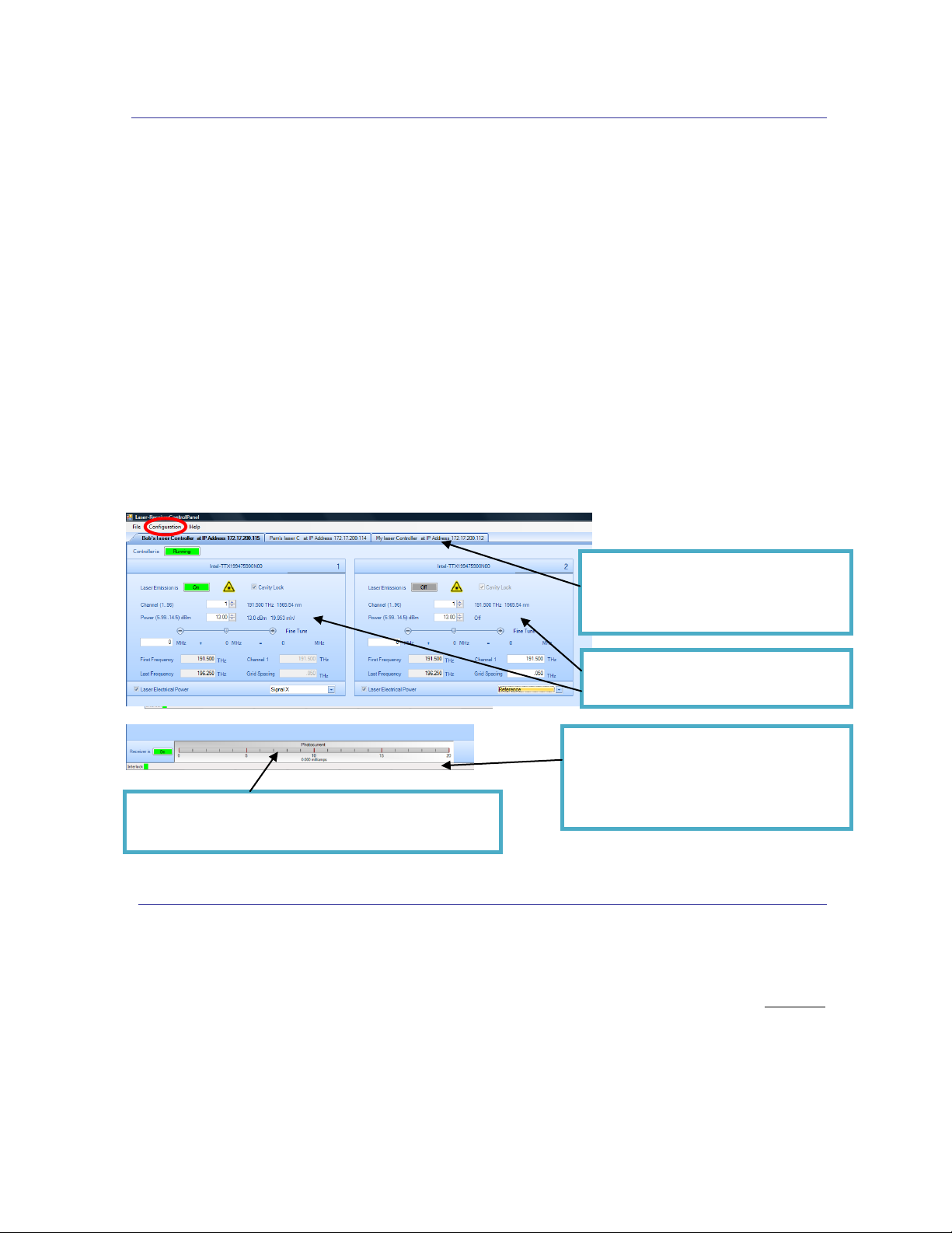
Receiver – The OM3x05 comes with receiver hardware.
This gauge displays the total photocurrent.
Controller – Each tab represents one
physical Laser Control device (for
example, the OM3X05) on the network.
Lasers – Each panel controls one
physical Laser on a specific controller.
The status bar will provide important
information about the overall state of the
communications with the controllers. Each
controller has a unique status bar.
6 Laser / Receiver Control Panel
The Laser-Receiver Control Panel (LRCP) application (LRCP) can be used to control a
variety of Integratable Tunable Laser Assembly (ITLA) lasers. The LRCP interface
simplifies the control of the lasers to relieve the user from the particulars of using the low
level ITLA command set. It allows the user to locate and configure all OM4000 Series
devices that are present on the local network. It also provides a Windows Communication
Foundation (WCF) service interface, allowing for the creation of Automated Test Equipment
(ATE) to interact directly with the controllers and lasers while LRCP is running.
There are three main components to the application: the controllers, the lasers and the
receiver. The following screen shot shows a LRCP that has three active controllers.
6.1 Device Setup and Auto Configure
The Device Setup screen can be accessed from the LRCP main menu under “Configura-
tion.” It will be necessary to enter this screen on initial setup of the controllers and anytime
network configuration changes and devices are moved to a new IP address. Clicking the
Auto Configure button will have the LRCP search for OM4000 Series devices and fill the
screen with information.
Tektronix OM4006/OM4106 Coherent Lightwave Signal Analyzer User Guide V1.5.1 10/24 ©2012 Page 70 of 148
Page 74

Auto configuration will return a list of all
available Optametra devices located on
Press the “Set” button if you change the
or type) of an individual device.
The friendly name is editable and may
more compatible with your
An important setting on the Device Setup screen that users will want to adjust is the Friendly
Name. Setting this value for each device will aid in the identification of the physical location
of the controllers as Friendly Names are retained and are tied to the corresponding MAC
Address. Make sure to exit the form by clicking the OK button to save changes.
network configuration (name, address,
be modified to uniquely identify
Optametra devices in a way that will be
The Set button is used to modify the addressing as described in the next section. It is not
necessary to use the Set button to change the Friendly Name.
Each device must be assigned an IP address in order to communicate with the device. How
you manage IP addresses in your network, namely with or without DHCP, will determine the
method in which you connect to the devices on your network.
6.2 Configuration on a network using DHCP
The default configuration uses DHCP to find OM4000 Series devices on the network. IP
Addresses will be “leased” to the devices for a period of time and then possibly reassigned
at a later date when the DHCP server decides it is time to reassign addresses. This is
similar to the way most cable modem ISPs work. The drawback to this method is that when
the IP address is reassigned the user must rerun auto configuration to reattach to the
proper IP Address. This is the simplest installation requiring the following steps.
o Open the menu “Configuration/Device Setup”
o Click on “Auto Configuration”
o All devices on the same subnet will be located and displayed.
NOTE: If you would like to assign the device a fixed IP in a DHCP environment you will
need to work with a network administrator to get fixed IP Addresses for devices.
Tektronix OM4006/OM4106 Coherent Lightwave Signal Analyzer User Guide V1.5.1 10/24 ©2012 Page 71 of 148
Page 75

6.3 Configuration on a network with no DHCP
In some cases the OM4000 Series devices will be installed on an isolated network
with fixed IP Addresses and no DHCP server. In order to talk to the device you
need to first set your local network to the device’s subnet address. As shipped, the
OM4000 Series devices will default to an IP Address of 172.17.200. xxx. This will not
necessarily be the same subnet as your local network. To get the OM4000 Series
device to communicate with your network you will need to do the following:
1) Attach a computer directly to the OM4000 Series controller via a cabled network
connection
2) Open the “Windows Control Panel”
3) Find the “Network and Sharing Center” and you should see this screen:
4) Click on “Manage Connections” and you will get the following screen:
Tektronix OM4006/OM4106 Coherent Lightwave Signal Analyzer User Guide V1.5.1 10/24 ©2012 Page 72 of 148
Page 76

5) Right-click to select the Properties for “Local Area Connection”, that is, the Ethernet
port that the OM4000 Series device is connect to
6) In the Properties window of the computer, select “Internet Protocol Version 4” and
then click “Properties”
7) Set the IP Address of the computer. Remember that the first three numbers of the
IP address entered here should match the first three numbers of the IP address used
by your OM4000 Series. This will put your computer on the same subnet as the
OM4000 Series device and make it visible to the “Auto-Configuration” process.
Tektronix OM4006/OM4106 Coherent Lightwave Signal Analyzer User Guide V1.5.1 10/24 ©2012 Page 73 of 148
Page 77

1. Auto Configure
2. IP Address
3. Gateway & Net
4. Set
8) Click OK to save the changes
Once the computer running LRCP has its network addressing configured, it will allow
LRCP’s Auto Configure button on the Device Setup screen to detect the controller so it can
be configured to work with your network. On the Device Setup screen do the following:
1. Click on “Auto Configure”. Your device should appear in the list with a valid MAC
address.
2. Edit the IP Address for the single device that will appear in the list. Set the address
to an IP Address that will be compatible with your network.
3. Set the Gateway and Net Mask (generally this requires you to speak with your
Network Admin to get the correct values.)
Note: If you change the Device IP Subnet Address to an address that is different than the
Subnet for the computer, the device will no longer be visible to the computer
once the Set button is pushed.
4. Click on the “Set” button
5. Unplug the network cable from between your computer and the OM4000 Series
device and connect the device to your network switch/router. It should now be
visible to the Auto Configure process and should show up with the same information
each time.
You can now set the device IP address to the desired IP network address and following the
same procedure set the Windows device address back to the same subnet address as the
device.
Tektronix OM4006/OM4106 Coherent Lightwave Signal Analyzer User Guide V1.5.1 10/24 ©2012 Page 74 of 148
Page 78

6.4 Connecting to your OM4000 Series device
Once configured, devices will appear as tabs on the main screen. They are listed with the
friendly name and IP address to allow for easy identification.
Up to four lasers will be displayed in a 2x2 grid. Lasers are numbered and once the
controller is brought Online the laser panels will populate with the laser manufacturer and
model number.
Once the user presses the button that reads Offline the button will change colors as the
control panel attaches to the OM4000 Series device. First, the button will turn yellow and
read “Connecting…” indicating that a physical network connection is being established over
a socket.
Second, the button will turn teal and read “Connected…”. This indicates that a session is
established between the device and Control Panel. Commands will be sent to initialize the
communications with the laser and identify their capabilities.
Finally, the button will turn bright green when the controller and lasers are ready for action.
Note: The button color scheme of bright green meaning running or active, grey meaning off
line or inactive and red indicating a warning or error state is consistent throughout
the application.
Once the controller tab is active and the laser panels have populated with the corresponding
laser information the user is free to put change the laser settings and/or turn the lasers on.
When the controller is first turned on the current state of the hardware is read to prepopulate the laser panel.
Tektronix OM4006/OM4106 Coherent Lightwave Signal Analyzer User Guide V1.5.1 10/24 ©2012 Page 75 of 148
Page 79

CAUTION
!
Any time you exit application, the current state of the lasers is
preserved, including the emission state.
If the lasers are used in conjunction with the OM4x06UI,
the laser usage type needs to be set using the dialog on
the lower right corner of each laser panel. This
OM4x06UI uses the setting to determine from which
laser frequency information is retrieved. A usage type
can only be selected once between all of the controllers
but you can have one usage type on one controller and another usage type on a second
controller.
Once laser emission is “On” the channel 1 and grid spacing settings become read only and
cavity lock becomes editable. Also the power goes from “off” to the actual power being read
from the laser. Readings are taking from the laser once per second.
Tektronix OM4006/OM4106 Coherent Lightwave Signal Analyzer User Guide V1.5.1 10/24 ©2012 Page 76 of 148
Page 80
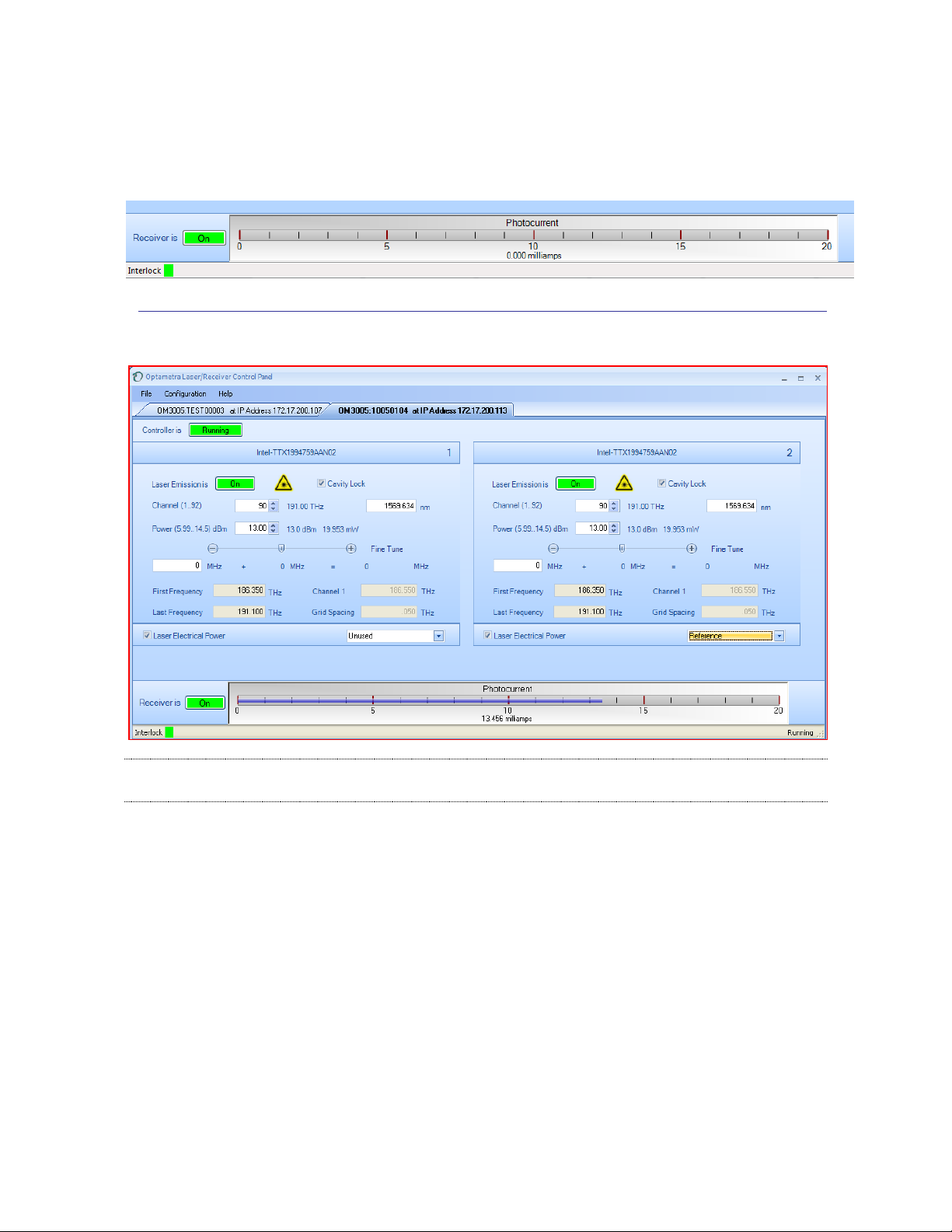
The receiver (shown below) is only functional on devices like the OM4000 Series that have
the appropriate hardware present. The receiver, when active, displays the total
photocurrent.
6.5 Setting laser parameters
Note: For all text field entries it is necessary to click away or press tab for the value en-
tered
Channel: Type a number or use the up/down arrows to choose a channel. The
range of channels available will depend on the type of laser, the First
Frequency, and the Grid. The finer the Grid, the more channels are
available for a given laser. The channel range is indicated next to the
word Channel. The laser channel can also be set by entering a
wavelength in the text box to the right of the channel entry. The laser will
tune to the nearest grid frequency.
Cavity Lock: The Intel/Emcore ITLA laser that is included in the OM4000 Series
receivers has the ability to toggle its channel lock function. Ordinarily,
Cavity Lock should be checked so that the laser is able to tune and lock
Tektronix OM4006/OM4106 Coherent Lightwave Signal Analyzer User Guide V1.5.1 10/24 ©2012 Page 77 of 148
Page 81

on to its frequency reference. However, once tuning is complete and the
laser has stabilized, this box can be unchecked to turn off the frequency
dither needed for locking the laser to its reference. The laser can hold its
frequency for days without the benefit of the frequency dither. The
OM4006 software will work equally well with the Cavity Lock dither on or
off.
Power: The allowed power range for the laser is listed after the word Power.
Type or use the up/down arrows to choose the desired laser power level.
Once entered, the actual laser power displayed to the right of the text box
should come into agreement with the desired power level.
Fine Tune: The Intel/Emcore lasers can be tuned off grid up to 12GHz. This can be
done by typing a number in the text box or by dragging the slider. The
sum of the text box and slider values will be sent to the laser. Once the
laser has accepted the new value it will be displayed after the ‘=’ sign.
First Frequency: Not settable. This is the lowest frequency that can be reached by the
laser.
Last Frequency: Not settable. This is the highest frequency that can be reached by the
laser.
Channel 1: Settable when emission is off. This is the definition of Channel 1.
Grid Spacing: Settable when emission is off. 0.1, 0.05 or 0.01 THz are typical choices.
Use 0.01THz if tuning to arbitrary (non-ITU-grid) frequencies. Using this
grid plus Fine Tune, any frequency in the laser band is accessible.
Laser Electrical
Power: This should normally be checked. Unchecking this box turns off electrical
power to the laser module. This should only be needed to reset the laser
to its power-on state, or to save electrical power if a particular laser is
never used.
Emission: Click to turn on or off front panel laser emission.
Tektronix OM4006/OM4106 Coherent Lightwave Signal Analyzer User Guide V1.5.1 10/24 ©2012 Page 78 of 148
Page 82

7 ATE (Automated Test Equipment) Interface
The OM4X06 Coherent Lightwave Signal Analyzer consists of two software programs, the
OM4000 Series User Interface (OUI) and the Laser Receiver Control Panel (LRCP) plus the
OM4000 Series Coherent Modulation Receiver. The OUI takes input from the user,
oscilloscope, and LRCP to process data received by the OM4000 Series and digitized by
the oscilloscope. The LRCP allows the user to control the OM4000 Series and
communicates status to the OUI. Both the OUI and the LRCP have two types of WCF
interfaces to allow control from a user application. Both types are provided to achieve full
functionality and compatibility with simple interfaces such as Matlab and via a client
application program.
7.1 LRCP ATE Interface
The Automated Test Equipment (ATE) interface exposes the LRCP functionality through a
Windows Communication Foundation (WCF) service. As the LRCP is used with all OM4000
Series laser controllers, its interface exposes more commands than those used by the
OM4x06 CLSA.
7.1.1 Basic/Advanced WCF Service Interface for the LRCP
The WCF services (basic and advanced) are available on port 9000 in the machine that is
running the LRCP. The service (basic and advanced) interface was developed for
incorporation into an ATE client application that can be developed in your choice of .NET
language, typically C# or VB.NET. Both services expose most of the functionality that is
available through the LRCP’s user interface.
The basic service, implemented using a wsBasicHTTPBinding, exposes the same subset
of commands as the advanced service. It was implemented using a simpler binding for
compatibility with applications like MATLAB (see Section 7.3.1 for Matlab usage details) or
Labview that only support the wsBasicHTTPBinding. The basic service is referenced at the
following URL:
http://localhost:9000/LaserReceiverControlPanel/Laser_ReceiverServiceBasic/
The advanced service, implemented using a wsHTTPBinding, (and which is not available
in Matlab) was developed for use with an ATE client application (see Section 7.4) and uses
Tektronix OM4006/OM4106 Coherent Lightwave Signal Analyzer User Guide V1.5.1 10/24 ©2012 Page 79 of 148
Page 83

events to provide a time-efficient interface. The advanced service is referenced at the
following URL:
http://localhost:9000/LaserReceiverControlPanel/Laser_ReceiverService/
Note: For safety reasons neither the basic or advanced services support the activation of
a laser; this must be done on the user interface.
7.1.2 LRCP Service Interface Function List
Refer to Section 6.5 for more information on the LRCP functionality of these exposed
functions. The following are the available commands in both the basic and advanced service
interfaces and demonstrate their functionality using the Matlab syntax:
int AvailableLasers(classname);
Returns the count of available lasers on the active controller.
Controller Types: All
Example: AvailableLasers(Obj);
Returns: ans = 2
bool Connect(classname);
Connects to the active controller, makes running.
Controller Types: All
Example: Connect(Obj);
Returns: ans = true Should see in LRCP screen
bool Disconnect(classname);
Disconnects from the currently active controller, takes offline.
Controller Types: All
Example: Connect(Obj);
Returns: ans = true Should see in LRCP screen
bool GetActualCavityLock(classname);
Gets the actual cavity lock state for the active controller / laser. Locked = True,
Controller Types: 3005, 3105, 2210, 2012
Example: GetActualCavity(Obj);
Returns: ans = true Should see in LRCP screen
double GetActualChannel(classname);
Gets the actual channel number for the active controller / laser.
Controller Types: 3005, 3105, 2210, 2012
Example: GetActualChannel(Obj);
Returns: ans = 1 Should see in LRCP screen
Tektronix OM4006/OM4106 Coherent Lightwave Signal Analyzer User Guide V1.5.1 10/24 ©2012 Page 80 of 148
Page 84

double GetActualChannel1(classname);
Gets the actual channel 1 frequency (in THz) for the active laser.
Controller Types: 3005, 3105, 2210, 2012
Example: GetActualChannel1(Obj);
Returns: ans = 191.5 Should see in LRCP screen
bool GetActualEmitting(classname);
Gets whether the Active Laser is emitting. Emitting = True.
Controller Types: 3005, 3105, 2210, 2012
Example: GetActualEmitting(Obj);
Returns: ans = true Should see in LRCP screen
short GetActualFineTuneFrequency(classname);
Gets the actual fine tune frequency (in MHz) of the active laser.
Controller Types: 3005, 3105, 2210, 2012
Example: GetActualFineTuneFrequency(Obj);
Returns: ans = 0 Should see in LRCP screen
double GetActualGridSpacing(classname);
Gets the actual grid spacing (in THz) of the active laser.
Controller Types: 3005, 3105, 2210, 2012
Example: GetActualFineTuneFrequency(Obj);
Returns: ans = 0.05 Should see in LRCP screen
double GetActualPower(classname);
Gets the actual power (in dBm) of the active laser.
Controller Types: 3005, 3105, 2210, 2012
Example: GetActualPower(Obj);
Returns: ans = 14.5 Should see in LRCP screen
double GetCalculatedFrequency(classname, laserusagetype
laserUsageType);
Searches all of the connected controllers for the first laser of the specified laser
usage type and returns the calculated frequency (in THz). Valid usage types are:
unused, signalx, signaly, signalxy, reference.
Controller Types: 3005, 3105, 2210, 2012, 5110
Example: GetCalculatedFrequency(Obj, reference);
Returns: ans = 191.5
string[] GetControllers(classname);
Returns a list (array) of controller devices (strings) that are being controlled by the
serving application.
Example: Controllers = GetControllers(Obj)
Returns: 'OM2210:Prototype1'
'OM2210:8180123'
'OM3105:6300121'
Tektronix OM4006/OM4106 Coherent Lightwave Signal Analyzer User Guide V1.5.1 10/24 ©2012 Page 81 of 148
Page 85

double GetFirstFrequency(classname);
Gets the first frequency (in THz) of the active laser.
Controller Types: 3005, 3105, 2210, 2012
Example: GetFirstFrequency(Obj);
Returns: ans = 191.5 Should see in LRCP screen
bool GetInterlock(classname);
Returns the current interlock state of the active controller. The normal, working state
is TRUE. If the interlock is disconnected from the back of the instrument or if the
instrument is powered off, this function will return FALSE.
Controller Types: All
Example: GetInterlock(Obj);
Returns: ans = true
string GetIP(classname);
Returns the IP Address (as a string) for the active controller.
Controller Types: All
Example: Address = GetIP(Obj);
Returns: Address = ‘172.17.200.114’
double GetLastFrequency(classname);
Gets the last frequency (in THz) of the active laser.
Controller Types: 3005, 3105, 2210, 2012
Example: GetLastFrequency(Obj);
Returns: ans = 196.25 Should see in LRCP screen
float GetPhotoCurrent(classname);
Gets the photocurrent (in mA) of the receiver in the active controller.
Controller Types: 3005, 3105
Example: GetPhotoCurrent(Obj);
Returns: ans = 11.034 Should see in LRCP screen
polarization GetPolarization(classname);
Returns the polarization state. Valid Polarization states are: filter1, filter2, unknown,
hardwarefailed.
Controller Types: 2210
Example: GetPolarization(Obj);
Returns: ans = filter2
bool InitializePolarization(classname);
Sets the initial polarization state. Returning True = Successful.
Controller Types: 2210
Example: InitializePolarization(Obj);
Returns: ans = true
Tektronix OM4006/OM4106 Coherent Lightwave Signal Analyzer User Guide V1.5.1 10/24 ©2012 Page 82 of 148
Page 86

bool SetActiveControllerByIPAddress(classname, string ipAddress);
Sets the active controller by IP Address. True = Successful.
Controller Types: All
Example: SetActiveControllerByIPAddress(Obj, ‘172.17.200.112’);
Returns: ans = true
GetIP(Obj);
Returns: ans = ‘172.17.200.112’
bool SetActiveControllerByName(classname, string activeController);
Sets the active controller by name. True = Successful.
Controller Types: All
Example: SetActiveControllerByName(Obj, 'OM3105:6300121')
Returns: ans = true
bool SetActiveLaser(classname, byte activeLaser);
Sets the active laser. Returning True = Successful.
Controller Types: 3105, 3005, 2210, 2012
Example: SetActiveLaser(Obj, 2);
Returns: ans = true
bool SetDesiredCavityLock(classname, bool desiredCavityLock);
Sets the desired cavity lock state for the active laser. 1 (True) = Locked. Returning
True = Successful.
Controller Types: 3005, 3105, 2210, 2012
Example: SetDesiredCavityLock(Obj, 1);
Returns: ans = true Should see in LRCP screen
bool SetDesiredChannel(classname, int desiredChannel);
Sets the desired channel number for the active laser. Returning True = Successful.
Controller Types: 3005, 3105, 2210, 2012
Example: SetDesiredChannel(Obj, 45);
Returns: ans = true Should see in LRCP screen
bool SetDesiredChannel1(classname, double desiredChannel1);
Sets the desired channel 1 frequency (in THz) for the active laser. Can only be set if
the active laser is NOT emitting. Returning True = Successful.
Controller Types: 3005, 3105, 2210, 2012
Example: SetDesiredChannel1(Obj, 192.5);
Returns: ans = true Should see in LRCP screen
bool SetDesiredEmittingOff(classname);
Sets the Active Laser to not emitting. Returning True = Successful.
Controller Types: 3005, 3105, 2210, 2012
Example: SetDesiredEmittingOff(Obj);
Returns: ans = true Should see in LRCP screen
Tektronix OM4006/OM4106 Coherent Lightwave Signal Analyzer User Guide V1.5.1 10/24 ©2012 Page 83 of 148
Page 87
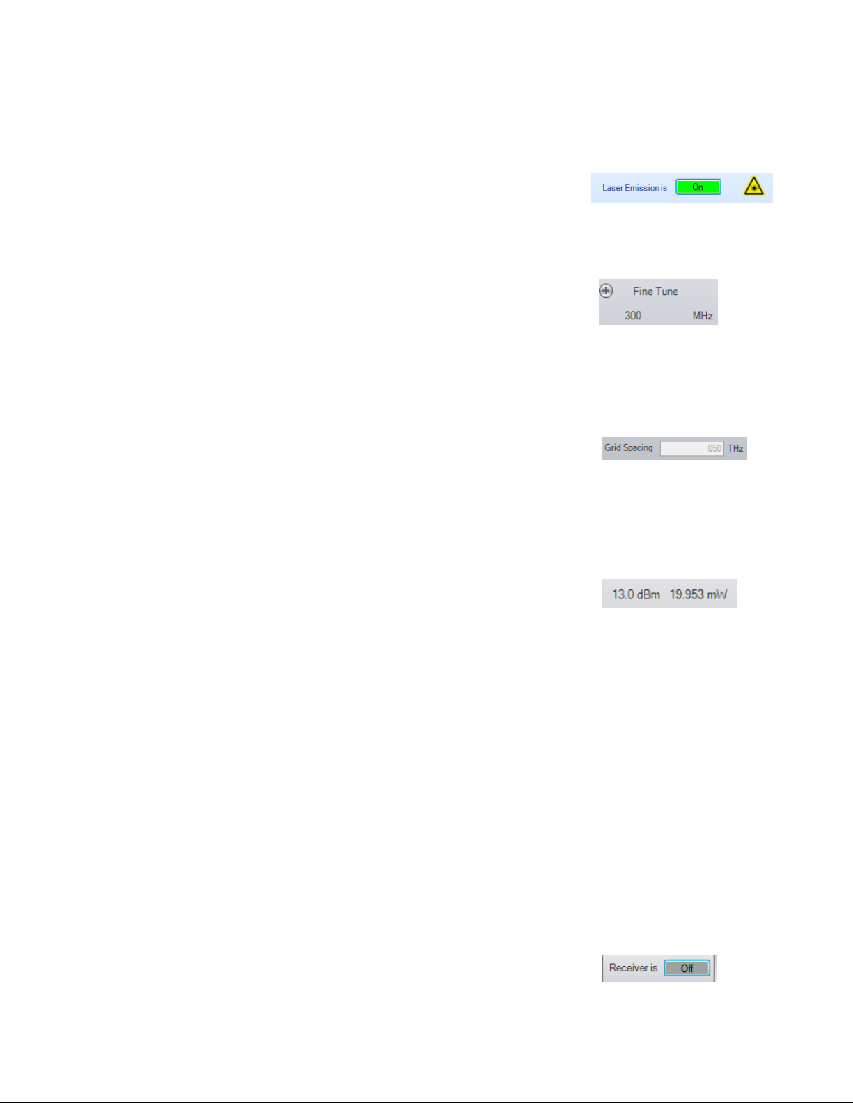
bool SetDesiredEmittingOn(classname);
Sets the Active Laser to emitting. Returning True = Successful.
Controller Types: 3005, 3105, 2210, 2012
Example: SetDesiredEmittingOn(Obj);
Returns: ans = true Should see in LRCP screen
bool SetDesiredFineTuneFrequency(classname, short
desiredFineTuneFrequency);
Sets the desired fine tune frequency (in MHz) of the active laser.
Controller Types: 3005, 3105, 2210, 2012
Example: SetDesiredFineTuneFrequency(Obj, 300);
Returns: ans = true Should see in LRCP screen
bool SetDesiredGridSpacing(classname, double desiredGridSpacing);
Sets the desired grid spacing (in THz) of the active laser. Can only be set if the
active laser is NOT emitting. Returning true = Successful.
Controller Types: 3005, 3105, 2210, 2012
Example: SetDesiredGridSpacing(Obj, 0.05,0);
Returns: ans = true Should see in LRCP screen
bool SetDesiredPower(classname, double
desiredPower, bool waitUntilFinished);
Sets the desired power (in dBm) of the active laser. For WaitUntilFinished, 0 (False)
= don’t wait. Returning True = Successful.
Controller Types: 3005, 3105, 2210, 2012
Example: SetDesiredPower(Obj, 13, 0);
Returns: ans = true Should see in LRCP screen
bool SetPolarizationIn(classname);
Puts both polarization filters in. Returning True = Successful.
Controller Types: 2210
Example: SetPolarizationIn(Obj);
Returns: ans = true
bool SetPolarizationOut(classname);
Puts both polarization filters out. Returning True = Successful.
Controller Types: 2210
Example: SetPolarizationOut(Obj);
Returns: ans = true
bool SetReceiverOff(classname);
Turns the receiver off in the active controller. Returning True = Successful.
NOTE: Ensure laser power is reduced to zero before doing this otherwise the
photoreceiver could be damaged.
Controller Types: 3005, 3105
Example: SetReceiverOff(Obj);
Returns: ans = true Should see in LRCP screen
Tektronix OM4006/OM4106 Coherent Lightwave Signal Analyzer User Guide V1.5.1 10/24 ©2012 Page 84 of 148
Page 88
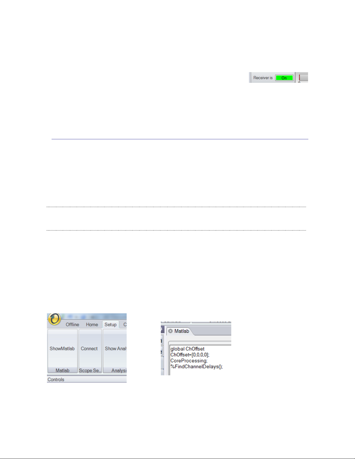
bool SetReceiverOn(classname);
Turns the receiver on in the active controller. Returning True = Successful.
Controller Types: 3005, 3105
Example: SetReceiverOn(Obj);
Returns: ans = true Should see in LRCP screen
void TogglePolarization(classname);
Toggles the polarization state by moving both filters to the opposite position.
Controller Types: 2210
Example: TogglePolarization(Obj);
7.2 OUI4006 ATE Interface
The Automated Test Equipment (ATE) interface exposes the OUI4006 user interface
functionality through one of two types of Windows Communication Foundation (WCF)
services. The WCF services (referred to as advanced and basic) are available on port 9200
in the machine that is running the OUI4006. This
Note: Because of an optimization in the OUI4006 application, when you attempt to read
variables from Matlab through this interface you must have the related plots displayed in the OUI4006 application or the values will not be calculated.
7.2.1 OUI Setup for ATE
There is some setup that is done in the OUI4006 application in preparation for an ATE
application. It is necessary to add function calls that perform additional calculations.
Variables used in these function calls and shared with the ATE application should be
declared as “global” in the Matlab Engine Command window as shown below with the
variable “ChOffset”:
The standard variables produced by CoreProcessing and any additional declared variables
will be repopulated each time a single is executed. After the data record is acquired from
Tektronix OM4006/OM4106 Coherent Lightwave Signal Analyzer User Guide V1.5.1 10/24 ©2012 Page 85 of 148
Page 89

the scope, the commands that are in the MatLab Engine Command window will be executed
using that data. The variables used in these executed commands will only be available until
the next single acquisition occurs. The ATE application should save the global variables to
local storage for processing before executing the next single acquisition. This process is
synchronized via a callback method or.NET event that is sent to the ATE application when
the processing of an acquisition is completed and the variables are ready for storage and
processing. Thus the Data/Variable process works like this:
A Single is executed;
Record/Block data is retrieved from the scope and saved to vBlock;
All commands in the MatLab Engine Command window are executed against the
acquired data record and all variables, both standard and global, are populated;
End of Block is triggered for each multiple of block size less than record size
End of Record is triggered
The ATE application should implement a callback handler for each event, block and/or
record, it is interested in. In general, ATE applications will probably have the block and
record size equal so the block and record events will be one for one. There are some
additional summary variables that are populated at the end of the record so it is best
practice to attach to the Record Event when block size is >= record size. The example of
this implementation is described in Section 7.4 under “Basic Method for getting MATLAB
variable values”
7.2.2 Basic/Advanced WCF Service Interfaces for the OUI4006
The basic service, implemented using a wsBasicHTTPBinding, exposes a smaller subset
of commands. It was implemented using a simpler binding for compatibility with applications
like MATLAB (see Section 7.3.1) or LabView that only support the wsBasicHTTPBinding.
The basic service can be referenced at the following URL:
http://localhost:9200/Optametra/OM4006/WCFServiceOM4006Basic/
The advanced service, implemented using a wsHTTPBinding and not available in Matlab,
uses events to provide a time-efficient interface. This service, which is only visible when the
OIU4006 application is run as administrator, has two components which reside at the
following URLs:
http://localhost:9200/Optametra/OM4006/WCFServiceOM4006/
http://localhost:9200/Optametra/OM4006/WCFServiceOM4006Bulk/
Tektronix OM4006/OM4106 Coherent Lightwave Signal Analyzer User Guide V1.5.1 10/24 ©2012 Page 86 of 148
Page 90

A wrapper DLL (OM4006ATEClient.DLL) has been supplied to simplify the interface to these
services. It is highly recommended that you use this DLL which is designed to deal with the
handshaking that is associated with working with events instead of interfacing directly to the
service. Section 7.4 explains how to reference this DLL in your client ATE Application.
Note: For safety reasons neither the basic or advanced services support the activation of
a laser; this must be done on the user interface.
7.2.3 OUI Basic & Advanced Service Interface Function List
Refer to Section 5 for more information on the OUI functionality of these functions both as
exposed by the simple http binding and the Client DLL. The following are the available
commands in both the basic and advanced service interfaces. These are the only OUI
functions that are available through the Matlab interface.
uint GetBlockSize(classname);
Returns the current block size from the OUI as an unsigned integer.
Example: GetBlockSize(Obj);
Returns: ans = 50000 Should see in OUI screen
uint GetRecordLength(classname);
Returns the current record length from the OUI as an unsigned integer.
Example: GetRecordLength(Obj);
Returns: ans = 1000 Should see in OUI screen
void SetBlockSize(classname, uint newBlockSize);
Sets the desired block size in the OUI as an unsigned integer for the next
acquisition.
Example: SetBlockSize(Obj, 2000);
void SetRecordLength(classname, uint newRecordLength);
Sets the desired record length in the OUI as an unsigned integer for the next
acquisition.
Example: SetRecordLength(Obj, 10000);
uint GetNumberOfAcquisitions(classname);
Returns the number of acquistion records taken by the OUI as an unsigned integer.
Example: GetNumberOfAcquisitions(Obj);
Returns: ans = 3578 Should see in OUI screen
uint GetNumberOfProcessedAcquisitions(classname);
Returns the number of processed acquistion records taken by the OUI as an
unsigned integer.
Example: GetNumberOfProcessedAcquisitions(Obj);
Tektronix OM4006/OM4106 Coherent Lightwave Signal Analyzer User Guide V1.5.1 10/24 ©2012 Page 87 of 148
Page 91

Returns: ans = 1357 Should see in OUI screen
bool IsRunning(classname);
Returns a boolean flag of the scope interface state; True = Acquisition is running
Example: IsRunning(Obj);
Returns: ans = true Should see in OUI screen
bool IsProcessing(classname);
Returns a boolean flag of the scope data state; True = Data is being processed
Example: IsProcessing(Obj);
Returns: ans = true Should see in OUI screen
bool IsAcquiring(classname);
Returns a boolean flag of the scope interface state; True = Data is being acquired
from the scope
Example: IsAcquiring(Obj);
Returns: ans = true Should see in OUI screen
bool IsCancelling(classname);
Returns a boolean flag of the scope interface state; True = Acquisition is being
cancelled
Example: IsCancelling(Obj);
Returns: ans = true Should see in OUI screen
bool IsReadyForSingle(classname);
Returns a boolean flag of the application state; True = Application is ready for
another single command
Example: IsReadyForSingle(Obj);
Returns: ans = true Should see in OUI screen
bool IsScopeConnected(classname);
Returns a boolean flag of the scope interface state; True = Application is connected
to a scope
Example: IsScopeConnected(Obj);
Returns: ans = true Should see in OUI screen
string GetScopeIDN(classname);
Returns a string containing the scope identifier
Example: GetScopeIDN(Obj);
Returns: ans = ‘TESTER’ Should see in OUI screen
string GetScopeAddress(classname);
Returns a string containing the scope IP address
Example: GetScopeAddress(Obj);
Returns: ans = ‘192.168.117.0’ Should see in OUI screen
Tektronix OM4006/OM4106 Coherent Lightwave Signal Analyzer User Guide V1.5.1 10/24 ©2012 Page 88 of 148
Page 92

double GetLOFreq(classname);
Returns a double containing the LO frequency
Example: GetLOFreq(Obj);
Returns: ans = 191.5 Should see in OUI screen
void SetLOFreq(classname, double loFreq);
Sets the desired LO Frequency as an double in the OUI for the next acquisition.
Note: This value may be overridden if the OUI retrieves the value from the LRCP
Example: SetLOFreq(Obj, 193.5);
void Connect(classname, string Address);
Connects the OUI to the specified scope having the valid VISA address.
Example: Connect(Obj, );
Returns: ans = ‘TESTER’ Should see in OUI screen
void Disconnect(classname);
Disconnects the application from the currently connected scope.
Example: Disconnect(Obj);
void Single(classname, int timeoutInMilliseconds);
Performs a single acquisition within the timeout period.
Example: Single(Obj,3000);
void DCCalib(classname);
Performs a basic DC calibration of the scope channels.
Example: DCCalib(Obj);
Note: All functions can throw an exception if there is an error. This fact should be used,
especially with functions that return void, to verify the correct operation of your ATE
program or script. For example, use the try-catch statement in Matlab to define how
certain errors are handled.
Tektronix OM4006/OM4106 Coherent Lightwave Signal Analyzer User Guide V1.5.1 10/24 ©2012 Page 89 of 148
Page 93

7.2.4 OUI Advanced Service Interface Function List
Refer to Section 5.2 for more information on the OUI functionality of these functions as
exposed by the Client DLL and Section 7.4 for examples of using these functions in an ATE
client application. The following commands are available in only the advanced service
interface:
public AnalysisParameters GetAnalysisParameters()
Returns a analysis parameters object containing the OUI variables
void SetAnalysisParameters(AnalysisParameters analysisParameters)
Sets the analysis parameters to new values
double GetDouble(string vname)
Returns the value of the passed variable as a double
bool GetBoolean(string vname)
Returns the value of the passed variable as boolean
bool[] GetArrayOfBoolean(string vname)
Returns the value of the passed variable as an array of boolean
double[] GetArrayOfDoubles(string vname)
Returns the value of the passed variable as an array of doubles
double GetComplexImaginary(string vname)
Returns the imaginary part of the specified complex number
double GetComplexReal(string vname)
Returns the real part of the specified complex number
double[] GetArrayOfComplexImaginary(string vname)
Returns an array of imaginary double values of the specified array of complex
numbers
void RegisterForBlockUpdate(MatLabVariable variable)
Registers a Matlab variable of interest for updating by Matlab at the end of block
processing
void RegisterForRecordUpdate(MatLabVariable variable)
Registers a Matlab variable of interest for updating by Matlab at the end of record
processing
void RegisterForBlockUpdate(List<MatLabVariable> variables)
Registers a list of Matlab variables of interest for updating by Matlab at the end of
block processing
void RegisterForRecordUpdate(List<MatLabVariable> variable)
Registers a list of Matlab variables of interest for updating by Matlab at the end of
record processing
void RegisterForBlockUpdate(string variableName)
Registers a variable for the block update by variable name
void RegisterForRecordUpdate(string variableName)
Registers a variable for the record update by variable name
Tektronix OM4006/OM4106 Coherent Lightwave Signal Analyzer User Guide V1.5.1 10/24 ©2012 Page 90 of 148
Page 94

string SendMatlabCommand(string matlabCommand)
This command is used to execuate a Matlab statement. NOTE: this can only be
used when the normal CoreProcessing is disabled or there will be contention with
the OUI4006's MATLAB engine. See Matlab section for usage.
void ExecuteMATLABCommands(string commandsToexecute)
This command is used to execute a block of matlab statements. NOTE: this can only
be used when the normal CoreProcessing is disabled or there will be contention with
the OUI4006's MATLAB engine. See Matlab section for usage.
void SetBlockCommands(string blockCommands)
Sets a string that has one or more Matlab commands that get run before block
processing occurs
void SetRecordCommands(string recordCommands)
Sets a string that has one or more Matlab commands that get run before record
processing occurs
void BlockProcessed(BlockProcessedEventArgs eventArgs)
Event Trigger that is executed when the OUI4006 application completes processing
of a block. You attach your event handler to this delegate and it is executed when
the event occurs.
void RecordProcessed(RecordProcessedEventArgs eventArgs)
Event Trigger that is executed when the OUI4006 application completes processing
of a record. You attach your event handler to this delegate and it is executed when
the event occurs.
string GetScopeState()
Returns a string containing a text description of the scope’s state. Valid states are:
Unknown, Disconnected, Connected, Acquiring
laserusagetype exposelaserusage()
Exposes the laser usage type to the OUI interface
bool ScreenShot(string filename)
Takes a snapshot of what the OUI has on the display, exactly like doing a
PrintScreen, and saves it the specified file
7.3 ATE Functionality in MATLAB
Matlab supports a limited subset of the OM4000 Series services, namely the Basic service.
This section describes how to create and address the functions from Matlab.
7.3.1 LRCP Control
The Laser/Receiver Control Panel communicates with other programs via port 9000 on the
computer running the Control Panel software. Matlab 2009a has built in capability that
Tektronix OM4006/OM4106 Coherent Lightwave Signal Analyzer User Guide V1.5.1 10/24 ©2012 Page 91 of 148
Page 95

makes control from Matlab easy if you are running the Feb 2010 or later release of the
Laser/Receiver Control Panel.
Note: Ensure that the LCRP is running before using this interface.
Initialize the interface in the MATLAB desktop command window with the following
commands:
url = 'http://localhost:9000/LaserReceiverControlPanel/Laser_ReceiverServiceBasic/?wsdl';
createClassFromWsdl(Url);
obj = Laser_ReceiverServiceBasic;
The first specifies the URL or path to a WSDL application programming interface (API) that
defines the web service methods, arguments, transactions. The second creates the new
class based upon that API and builds a series of M-Files for accessing the Laser/Receiver
Control Panel service. The third instantiates the object class name and opens a connection
to the service. These commands only need to be run anytime the service interface
(available methods) changes. To get an up-to-date listing of methods for the service type
the following:
methods(obj)
Matlab should return the same functions as given in Section 7.1.2 and any new functions
that have been added. These functions are self-documented when they are generated. By
enabling the Matlab help window, you can find out the function’s parameters by typing the
function name followed by a “(“ and waiting for the help to pop up.
7.3.2 OUI4006 Control in MATLAB
The OM4000 Series OUI communicates with other programs via port 9200 on the computer
running the OUI software.
Note: Ensure that the OUI is running before using this interface.
Initialize the interface in the MATLAB desktop command window with the following
commands:
url = 'http://localhost:9200/Optametra/OM4006/WCFServiceOM4006Basic/?wsdl';
createClassFromWsdl(Url);
obj = WCFServiceOM4006Basic;
The first command specifies the URL or path to a WSDL application programming interface
(API) that defines the methods, arguments, and transactions for the OUI web service. The
Tektronix OM4006/OM4106 Coherent Lightwave Signal Analyzer User Guide V1.5.1 10/24 ©2012 Page 92 of 148
Page 96

second command creates the new class based upon that API and builds a series of M-Files
for accessing the OUI basic service. The third instantiates the object class name and opens
a connection to the OUI basic service. These commands need to be run whenever the
service interface (available methods) change. To get an up-to-date listing of methods for the
OUI basic service type the following:
methods(obj)
Matlab should return the same functions as given in Section 7.3.2 and any new functions
that have been added. These functions are self-documented when they are generated. By
enabling the Matlab help window, you can find out the function’s parameters by typing the
function name followed by a “(“ and waiting for the help to pop up.
7.4 Building an OM4006 ATE Client in VB.NET
The following document explains how to build an OM4006 ATE Client application in VB.NET
using the OM4006ATEClient .NET Assembly provided with the OUI4006 ATE Toolkit. The
ATE interface to OUI4006.EXE is implemented using several WCF Services. There are
actually two ways that a ATE client application can interface to the WCF Services. One is to
create a service reference in a VB Project that talks directly to the WCF Service. The other
is to add a reference to the OM4006ATEClient .NET assembly. The preferred method is to
use the OM4006ATEClient .NET assembly and this document will explain how to implement
that method.
WCF Service Background
The OUI4006 application exposes functionality using several WCF services. The
OM4006ATEClient assembly uses two of those WCF services as detailed in Section 7.2.2
to convey detailed processing information and expose a variety of control to the ATE Client
application. WCFServiceOM4006 exposes most of the functionality, including
asynchronous events. WCFServiceOM4006Bulk exposes bulk data methods to retrieve
large arrays of data. Aside from the information about the location of the services (added to
the APP.Config file, see below) the client that uses the OM4006Client.NET assembly really
doesn’t need to worry about any of the details of the services.
Tektronix OM4006/OM4106 Coherent Lightwave Signal Analyzer User Guide V1.5.1 10/24 ©2012 Page 93 of 148
Page 97
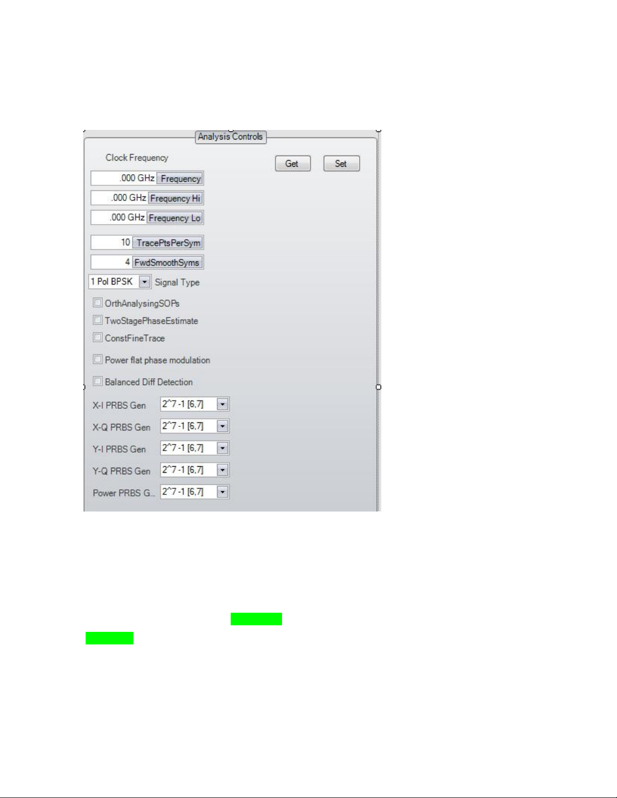
The following user control (ucAnalysisParameters) is provided in OM4006ATEClient for use
in ATE client applications.
Add Service References in APP.CONFIG file of the ATE Client application
The OM4006Client assembly will need to know where to look for the WCF Services. Those
services can reside on the local machine or on a remote computer. The information is used
by the OM4006ATEClient assembly to establish a connection to the host OUI4006
application. Please note the “localhost” below. If the computer is not local then replace
”localhost” with the name of the remote machine, for example “DavesAsus”. Adding the
XML below to your APP.CONFIG file will define two service references running on the local
machine.
Tektronix OM4006/OM4106 Coherent Lightwave Signal Analyzer User Guide V1.5.1 10/24 ©2012 Page 94 of 148
Page 98

<system.serviceModel>
<bindings>
<basicHttpBinding>
<binding name="BasicHttpBinding_IWCFServiceOM4006Bulk"
closeTimeout="00:10:00" openTimeout="00:10:00"
receiveTimeout="00:10:00" sendTimeout="0010:00"
maxBufferSize="1000000000" maxBufferPoolSize="1000000000"
maxReceivedMessageSize="1000000000" transferMode="Streamed"
useDefaultWebProxy="true">
<readerQuotas maxDepth="1000000000"
maxStringContentLength="1000000000" maxArrayLength="1000000000"
maxBytesPerRead="1000000000" maxNameTableCharCount="1000000000" />
</binding>
</basicHttpBinding>
<wsDualHttpBinding>
<binding name="WSDualHttpBinding_IWCFServiceOM4006"
closeTimeout="00:10:00" openTimeout="00:01:00"
receiveTimeout="00:10:00" sendTimeout="00:10:00"
bypassProxyOnLocal="false" transactionFlow="false"
hostNameComparisonMode="StrongWildcard" maxBufferPoolSize="524288"
maxReceivedMessageSize="65536" messageEncoding="Text"
textEncoding="utf-8" useDefaultWebProxy="true">
<readerQuotas maxDepth="32" maxStringContentLength="8192"
maxArrayLength="16384" maxBytesPerRead="4096"
maxNameTableCharCount="16384" />
<reliableSession ordered="true" inactivityTimeout="00:10:00" />
<security mode="Message">
<message clientCredentialType="Windows"
negotiateServiceCredential="true"
algorithmSuite="Default" />
</security>
</binding>
</wsDualHttpBinding>
</bindings>
<client>
<endpoint
address="http://localhost:9200/Optametra/OM4006/WCFServiceOM4006/"
binding="wsDualHttpBinding"
bindingConfiguration="WSDualHttpBinding_IWCFServiceOM4006"
contract="WCFServiceOM4006.IWCFServiceOM4006"
name="WSDualHttpBinding_IWCFServiceOM4006">
<identity>
<dns value="localhost" />
</identity>
</endpoint>
<endpoint
address="http://localhost:9200/Optametra/OM4006/WCFServiceOM4006Bulk/"
binding="basicHttpBinding"
bindingConfiguration="BasicHttpBinding_IWCFServiceOM4006Bulk"
contract="WCFServiceOM4006Bulk.IWCFServiceOM4006Bulk"
name="BasicHttpBinding_IWCFServiceOM4006Bulk">
<identity>
<dns value="localhost" />
</identity>
</endpoint>
</client>
</system.serviceModel>
Tektronix OM4006/OM4106 Coherent Lightwave Signal Analyzer User Guide V1.5.1 10/24 ©2012 Page 95 of 148
Page 99
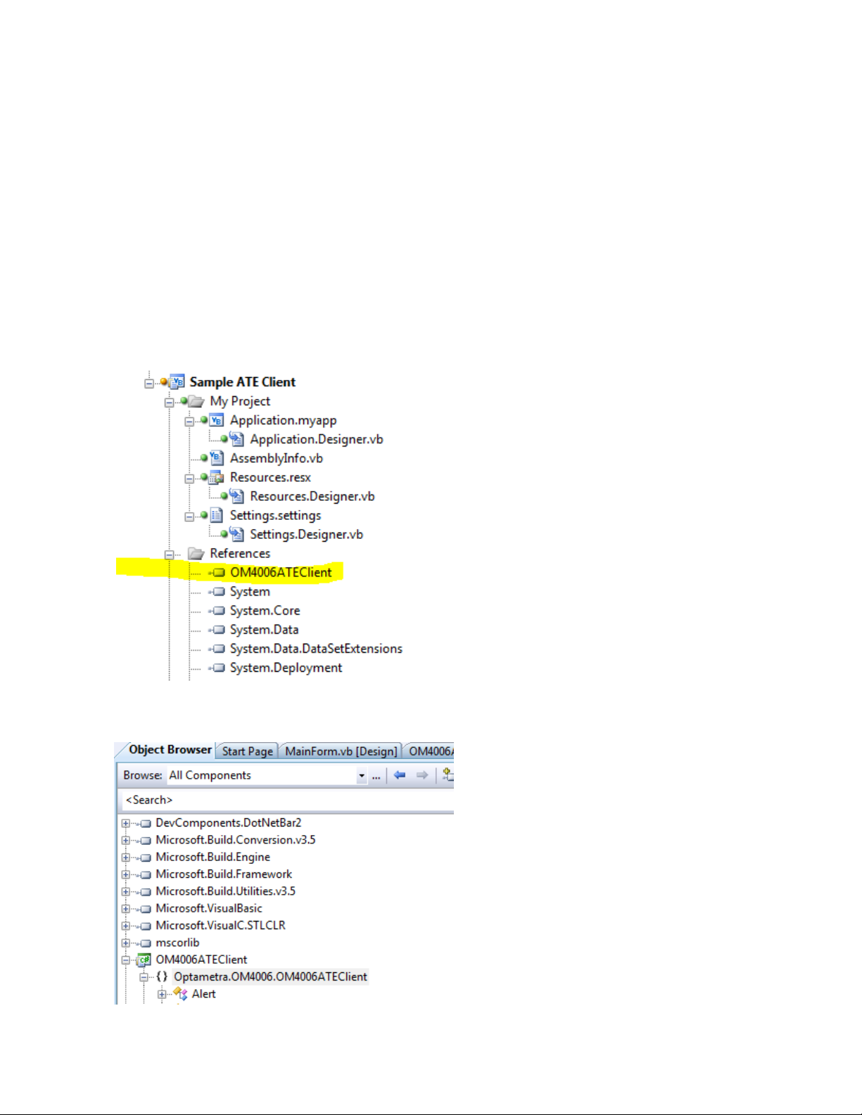
OM4006ATEClient .NET Assembly
This assembly includes a basic interface for retrieving MATLAB variable values and an
object oriented interface that includes specialized .NET classes for all of the OM4000 Series
specific variables. This interface allows a client application to read and set all analysis
parameters such as Block Size and Record Length. It also has the ability to connect or
disconnect to/from a scope based on IP address as well as trigger single acquisitions.
Additionally, the application can register for events that occur at the end of blocks and
records.
To get started add the following (highlighted in yellow) reference to your ATE Client
application. The file can be found in the folder where OUI4006 is installed.
Once the reference is added it can be browsed to understand the available functionality.
Double click on the reference to bring up the Object browser.
Tektronix OM4006/OM4106 Coherent Lightwave Signal Analyzer User Guide V1.5.1 10/24 ©2012 Page 96 of 148
Page 100

Scroll down from Optametra.OM4006.OM4006ATEClient and double-click on OM4006ATEClient:
The right pane on the object browser should look like the following image:
Tektronix OM4006/OM4106 Coherent Lightwave Signal Analyzer User Guide V1.5.1 10/24 ©2012 Page 97 of 148
 Loading...