Tektronix OM1106 Primary User

Download

OM1106 Optical Modulation Analysis Software

ZZZ

Version 2.2.x and Below

User Manual

*P077109302*

077-1093-02

OM1106 Optical Modulation Analysis Software

ZZZ

Version 2.2.x and Below

User Manual

Click the following link to protect your product.

► www.tek.com/register

www.tek.com

077-1093-02

Copyright © Tektronix. All rights reserved. Licensed software products are owned by Tektronix or its subsidiaries or suppliers, and are protected by national copyright laws and international treaty provisions.

Tektronix products are covered by U.S. and foreign patents, issued and pending. Information in this publication supersedes that in all previously published material. Speciﬁcations and price change privileges reserved.

TEKTRONIX and TEK are registered trademarks of Tektronix, Inc.

MATLAB is a registered trademark of The MathWorks, Inc.

Other product and company names listed are trademarks and trade names of their respective companies.

Contacting Tektronix

Tektronix, Inc. 14150 SW Karl Braun Drive P.O. B o x 5 0 0 Beaverton, OR 97077 USA

For product information, sales, service, and technical support:

In North America, call 1-800-833-9200. Worldwide, visit www.tek.com to ﬁnd contacts in your area.

Table of Contents

Preface ............................................................................................................. vii

Related documents.................. ................................ ................................ ......... vii

Install software........................... ................................ .................................. ......... 1

PC hardware and software requirements........... ................................ ......................... 1

MATLAB

Set Windows 7 user account setting before installing software . . ..... . ..... . . ... . . . ..... . ..... . ..... . . .. 2

Required software to install................................ .................................. ................. 2

To install MATLAB software............... ................................ ............................. 3

To install TekVISA software ............................................................................ 3

To install power meter software (for RXTest and OM2210) .................. ....................... 4

To install OMA software........ ................................ .................................. ....... 5

To install Scope Service Utility (SSU) software. . ..... . ..... . ..... . ..... . ..... . ..... . ..... . ..... . ..... 7

Updating existing OMA (OUI) installations................................................................ 9

Verify software installation ........ ................................ ................................ .......... 10

Further information......... ................................ .................................. ................ 11

Verify or set OM series instrument IP address ................................................................. 13

Verify OM instrument connectivity on DHCP-enabled network ...... .................................. 13

Set OM instrument IP address for use on non-DHCP network ............ .............................. 14

OM1106 Optical Modulation Analysis (OMA) user interface ............................................... 19

OMA user interface elements ............................................................................... 21

The Menu ribbon.............................................................................................. 21

The Plots panel................................................................................................ 22

The global Controls panel ................................................................................... 28

The Setup tab controls ............................................................................................ 29

Scope Setup controls ............................ ................................ ................................ .. 29

Scope Connect button ........................................................................................ 29

Use VISA control (Scope Setup)...... .................................. ................................ .... 31

Auto Scale and DC Calib button............................................................................ 34

Scope & Receiver Deskew button .......................................................................... 34

Optical Connect.................................................................................................... 36

Optical Control Panel (LRCP) ................................................................................... 38

Connect to an OM instrument ....... ................................ ................................ ........ 39

The Laser controls ............................................................................................ 40

The Modulator controls .... .................................. ................................ ................ 42

The Driver Amp controls .............. ................................ .................................. .... 47

MATLAB Command/Response tab ............................................................................. 48

Analysis Parameters control and conﬁguration tab .......... ................................ .................. 50

Front end ﬁltering............................................................................................. 57

LMS ﬁltering...... .................................. ................................ .......................... 59

software requirements........................................................................... 2

OM1106 Analysis Software User Manual i

Table of Contents

Direct assignm

Direct assignment of pattern variables when not using a PRBS......................................... 62

Example capturing unknown pattern ....................................................................... 63

The Multicarrier Setup window . . .... . . .... . . .... . . .... . . .... . . .... . . .... . . .... . ..... . ..... . ..... . ..... . ..... . ... 65

Multicarrier channel list... . ... . . . .... . ..... . ..... . .... . ..... . ..... . .... . . .... . ..... . ..... . .... . ..... . ..... . .. 66

Multicarrier display layout. . . .... . . .... . ..... . ..... . ..... . ..... . ..... . ..... . ..... . ..... . ... . . ..... . ..... . .... 67

The Receiver Test conﬁguration tab............................................................................. 68

To perform a receiver test.................................................................................... 71

State controls ................................. ................................ ................................ ...... 80

The Home tab .................. ................................ ................................ .................... 81

Constellation plots............ .................................. ................................ .............. 81

Eye plots ....................................................................................................... 86

BER plots...................... ................................ .................................. .............. 91

Poincaré plots . ................................ ................................ ................................ 92

Q factor plots .............................. ................................ ................................ .... 94

Spectrum plots ................................................................................................ 95

Measurement plots.................. ................................ ................................ ........ 100

Signal vs. Time plot ........................................................................................ 103

Layout controls.......... .................................. ................................ .................. 106

The Calibrate tab ................................................................................................ 107

Enable Sliders (signal delay ﬁne adjusts) (RT).................. ................................ ........ 107

DC Calibration (real-time oscilloscopes) . ..... . ..... . ..... . ...... . ...... . . ..... . . ..... . . ..... . . ..... . . .. 108

Get Calibration Files ............... ................................ ................................ ........ 108

The Ofﬂine tab ................................................................................................... 109

The Alerts tab .......... .................................. ................................ ........................ 111

The About tab .................................................................................................... 113

The global Controls panel ........ ................................ ................................ .............. 115

Appendix A: Hybrid calibration (RT)... ................................ ................................ ...... 117

Appendix B: OM5110 information ............................................................................ 121

Theory of operation......................................... .................................. .............. 121

Appendix C: OM2210 information............................................................................ 123

Product description . .................................. ................................ ...................... 123

Appendix D: Connection diagrams ............................................................................ 125

OM4000-series equipment setup........................ ................................ .................. 125

OM2210 equipment setup ................................................................................. 131

OM2012 equipment setup ................................................................................. 133

Appendix E: Receiver Test ..................................................................................... 135

Receiver Test overview .............. .................................. ................................ .... 135

Receiver test setup.................. ................................ ................................ ........ 137

Software operation.......................................................................................... 138

Test vs modulation frequency ............................................................................. 141

ent of pattern variables ....................... ................................ .............. 62

ii OM1106 Analysis Software User Manual

Table of Contents

Test v s Wave len

Receiver Test ATE Commands............................................................................ 146

Appendix F: DSA8300 equivalent-time (ET) oscilloscope operation ..... . ..... . ..... . ..... . ..... . ..... . . 149

Conﬁguring the software (ET) .... ................................ .................................. ...... 149

OMA and equivalent-time (ET) instruments ............................................................ 151

Calibration and adjustment (ET) ...... .................................. ................................ .. 153

Taking measurements (ET) .................... ................................ ............................ 163

OMA Controls panel (ET) ................................................................................. 163

Analysis Parameters window (ET)............................ .................................. .......... 164

Appendix G: Conﬁguring two Tektronix 70000 series oscilloscopes.................................. .... 167

Oscilloscope settings ..... . ..... . ..... . ... . . ..... . ..... . ..... . .... . . .... . ..... . ..... . ..... . ..... . .... . ..... . 170

OMA settings for two-oscilloscope operation . ..... . ..... . ... . . . .... . ..... . ..... . ..... . ..... . ..... ..... . 172

Appendix H: Alert codes ....................................................................................... 175

Appendix I: MATLAB CoreProcessing software guide....................................... .............. 177

MATLAB interaction with OMA ....... ................................ .................................. 177

MATLAB variables......................................................................................... 178

MATLAB functions ...... ................................ .................................. ................ 179

Signal processing steps in MATLAB CoreProcessing.............................. .................... 180

MATLAB block processing ............................................................................... 185

Alerts management ......................................................................................... 186

Appendix J: The ATE (automated test equipment) interface ............................................... 189

The LRCP ATE interface .................. .................................. .............................. 189

The OMA ATE interface................................................................................... 203

Building an OMA ATE client in VB.NET ............................................................... 215

Appendix K: MATLAB CoreProcessing function reference............................................ .... 221

AlignTribs ................................................................................................... 221

ApplyPhase........................ ................................ .................................. ........ 224

ClockRetime................... ................................ ................................ .............. 225

DiffDetection................................................................................................ 226

EstimateClock............................................................................................... 227

EstimatePhase ............................................................................................... 229

EstimateSOP .. .................................. ................................ ............................ 230

MaskCount .................................................................................................. 231

GenPattern ................................................................................................... 232

Jones2Stokes ...... ................................ .................................. ........................ 233

JonesOrth .................................................................................................... 234

LaserSpectrum .............................................................................................. 234

QDecTh ...................................................................................................... 235

zSpectrum.................................................................................................... 236

Appendix L: MATLAB variables used by CoreProcessing ................................................. 237

MATLAB input variables ................................ ................................ .................. 237

gth ................. ................................ ................................ ........ 145

OM1106 Analysis Software User Manual iii

Table of Contents

MATLAB calcula

Appendix M: Managing data sets with record length > 1,000,000......................................... 239

Saving intermediate data sets: examples................................................................. 239

Examples of save statements for unique ﬁle name.................................. .................... 239

Examples of if-statements and alerts to trigger a save ................................ .................. 240

Index

ted variables .................. ................................ .......................... 238

iv OM1106 Analysis Software User Manual

List of Figures

Figure 1: The OMA screen with plots and measurements .......... ................................ .......... 19

Figure 2: Default OMA startup screen.................... ................................ ...................... 21

Figure 3: LRCP tab showing OM5110 controls................................................................ 38

Figure 4: LR

Figure 5: Multicarrier setup window . ..... . ..... ..... . ..... . .... . . .... . ..... . ... . . ..... . ..... . .... . ..... . ..... . . 65

Figure 6: Multicarrier constellation plots ..... . ..... . .... . ..... . ..... . .... . . .... . ..... . ..... . .... . ..... . ..... . .. 85

Figure 7: Multicarrier spectrum context menu . . .... . ... . . ..... ..... . .... . ..... ..... . .... . ... . . ... . . ..... ..... . 96

Figure 8: Multicarrier spectrum plot ..... . ... . . ..... . ..... . .... . ..... . ... . . ..... . ..... . .... . ..... . ... . . ..... . ... 98

Figure 9: Multicarrier spectrum plot details ..... . ..... . .... . ..... ..... . .... . ... . . ... . . ..... ..... . .... . ..... .... 99

Figure 1

Figure 11: Real-time (RT) oscilloscope setup diagram: Tektronix DSO/MSO70000C/D/DX series and

OM4245 Optical Modulation Analyzer .... ................................ .............................. 125

Figure 12: Real-time (RT) oscilloscope setup diagram: <80 GBaud single polarization testing using

DPO77002SX ATI oscilloscopes and OM4245 Optical Modulation Analyzer . . ..... . ..... . .... . ... 126

Figure 13: Real-time (RT) oscilloscope setup diagram: <60 GBaud dual polarization testing using

DPO77

Figure 14: Real-time (RT) oscilloscope setup diagram: 400G (<80 GBaud) dual-polarization signal testing

using DPO77002SX ATI oscilloscopes and OM4245 Optical Modulation Analyzer... . ..... . ..... 128

Figure 15: Equivalent-time (ET) oscilloscope setup diagram: DSA8300 and OM4245 ..... . .... . . .... 129

Figure 16: Heterodyne coherent receiver test system diagram ................... .......................... 136

Figure 17: Relay connections on the S46T when used with the SX70000................................ 136

gure 18: ChDelay(2) off by 2 ps causes curvature on constellation and signal on Q-Eye for 28 Gbps

BPSK......................................................................................................... 155

Figure 19: When adjusting the middle slider, watch the Y-Eye and Y-Const to minimize the signal in the

Y-polarization . ................................ .................................. ............................ 157

Figure 20: Final channel delay values provide only noise in Y polarization ..................... ........ 158

CP tab showing OM4200 controls.................................. .............................. 38

0: OM5110 block diagram................ ................................ ............................ 121

002SX ATI oscilloscopes and OM4245 Optical Modulation Analyzer . . .... . . .... . ..... . ... 127

OM1106 Analysis Software User Manual v

Table of Contents

List of Tables

Table 1: Oscilloscope connectivity capabilities (TekVISA vs. Scope Service Utility) . ..... . ..... . ..... . . 33

Table 2: La s

Table 3: OM5110 Modulator controls (Auto-Set mode) (LRCP) ............................................ 43

Table 4: OM5110 Modulator controls (manual mode) (LRCP) .............................................. 44

Table 5: OM5110 Driver Amp controls (LRCP)........................... ................................ .... 47

Table 6: Analysis Parameters ﬁelds ............................................................................. 50

Table 7: RXTest parameters...................................................................................... 69

Table 8: R

Table 9: RxTest: Wavelength sweep plots ........................ .................................. ............ 76

Table 10: RxTest: Modulation Frequency sweep plots........................................................ 79

Table 11: Constellation plots..................................................................................... 81

Table 12: Eye plots................ ................................ ................................ ................ 86

Table 13: BER plots............................................................................................... 91

Table

Table 15: Q factor plots........................................................................................... 94

Table 16: Spectrum plots . .................................. ................................ ...................... 95

Table 17: Multicarrier spectrum menu choices (right-click). . ..... . ... . . . .... . . .... . ..... . ..... . ..... . ..... . . 96

Table 18: Multicarrier spectrum controls .... . ..... . ... . . ..... . ..... . ... . . ..... . ... . . . .... . ..... . ... . . ..... . .... 97

Table 19: Measurement plots................................................................................... 100

ble 20: Signal vs. Time plot ......... ................................ ................................ ........ 103

Table 21: Ofﬂine controls .. ................................ .................................. .................. 109

Table 22: Controls panel elements........................... ................................ .................. 115

Table 23: Record length and block interaction behavior .................................................... 116

Table 24: Receiver Test conﬁgurations and channel mappings ............................................ 140

Table 25: Test properties........................................................................................ 143

Table 26: Alert code descriptions........ ................................ ................................ ...... 175

er controls (LRCP).................................................................................. 41

eceiver test readout tabs .................. ................................ ............................ 74

14: Poincaré plots .......................................................................................... 92

vi OM1106 Analysis Software User Manual

Preface

Related documents

This documen

t describes how to install, conﬁgure, and operate the OM1106

Optical Modulation Analyzer (OMA) software version 2.2.x and lower.

Tektronix part

Document

OM4245, OM4225 Optical Modulation Analyzer Installation and Safety

ons

Instructi

OM2210 Coherent Receiver Calibration Source Installation Safety Instructions

OM2012 nLaser Tunable Laser Source Installation and Safety Instructions

OM5110 4 Instructions

Tektro Declassiﬁcation and Security Instructions

Avert OM4006D, O M2210, OM2012 et OM5110)

6 GBaud Multi-Format Optical Transmitter Installation and Safety

nix OM5000, OM4000, OM2000 Series Optical Modulation Instruments

issements - Mises en garde (manuels OM4245, OM4225, OM4106D,

number

071-3414-xx

071-3050-xx

071-3154

071-3203-xx

077-0992-xx

071-3184-xx

-xx

OM1106 Analysis Software User Manual vii

Preface

viii OM1106 Analysis Software User Manual

Install software

The OM1106 Optical Modulation Analyzer software (referred to as OMA in this document) provides an ideal platform for research and testing of coherent optical systems. It o

ffers a complete software package for acquiring, demodulating, analyzing, and visualizing complex modulated systems with an easy-to-use user interface. The software performs all calibration and processing functions to enable real-time burst-mode constellation diagram display, eye diagram display, Poincaré sphere display, and BER evaluation.

This section descr

ibes how to install and conﬁgure the OMA software and OM

series instruments to correctly communicate with each other.

PC hardware and software requirements

The following are the PC requirements needed to install and run the OMA software to control the OM4000 and OM2000 series instruments. The term PC applies to a supported oscilloscope, PC, or laptop on which the OMA and other required software is installed, and t a local network.

Item Description

Operating system

Windows .NET version (32– or 64-bit Windows)

Processor

RAM

Hard Drive Space

Video Card

U.S.A. Microsoft Windows 7 (32- or 64-bit), with latest updates and service packs installed

4.51 or later

NOTE. The OMA install process updates the .NET software if required.

Intel i7, i5 or equivalent; min clock speed 2 GHz

Minimum: Intel Pentium 4 or equivalent

Minimum: 4 GB

64-bit releases beneﬁt from as much memory as is available

Minimum: 20 GB

>300 GB recommended for large data sets

nVidia dedicated graphics board with 512+ MB minimum graphics memory

hat is connected to OM instruments over

NOTE. OMA will run with video cards other than nVidia. However, color

gradient display (for plots that support that feature) and some advanced plot features are only available when running OMA on an oscilloscope or PC that has an nVidia graphics card installed.

Download and install the latest drivers available from the video card manufacturer. There may be newer drivers available even if Windows says the drivers are up to date.

Networking

Display

Gigabit Ethernet (1 Gb/s) or Fast Ethernet (100 Mb/s)

20” minimum ﬂat screen recommended for displaying multiple graph types

OM1106 Analysis Software User Manual 1

Install software

Item Description

Other Hardware

Adobe Reader

2 USB 2.0 ports

Adobe reader used for viewing PDF format ﬁles

MATLAB®sof

Set W

indows 7 user account setting before installing software

tware requirements

The OMA software requires the appropriate version of the MathWorks, Inc. MATLAB product so MATLAB version for your PC (www.mathworks.com).

OMA requi

NOTE. OMA uses the most recently installed MATLAB software. If you need to

revert to a previously installed Matlab, please see further instructions below.

Default Windows 7 user account settings interfere with OMA IVI/Visa operation. To ﬁx this, do the following before installing any software:

ftware media. Please contact The MathWorks, Inc. to obtain the correct

res the following versions of MATLAB:

For Microsoft Windows 7 (64-bit), U.S.A. version: MATLAB v

For MicrosoftWindows 7 (32-bit) U.S.A. version: MATLAB

Click Start > Control Panel > User Accounts.

software for performing analysis. MATLAB is not included on the

ersion 2011b (64-bit) or 2014a (64-bit)

version 2009a (32-bit)

Click Change User Account Control settings and set the notify control to Never notify.

quired software to install

Software required on the

Install the following software on the controller PC in the order listed.

controller PC

NOTE. Install all software as an Administrator.

CAUTION. Do not insert the product USB HASP key when installing the following

software. Only install the HASP key after all software is installed and you are ready to run the OMA software.

2 OM1106 Analysis Software User Manual

Install software

Software required on the

oscilloscope

To install MATLAB

software

1. MATLAB: Requir

installing OMA. (See page 3.)

2. TekVISA: Requ

series oscilloscopes.

NOTE. Do not load TekVISA for MSO/DSO70000C/D/DX/SX series real-time

(RT) oscilloscopes or the DSA8300 equivalent-time (ET) oscilloscope. These oscilloscopes use the Scope Service Utility (SSU).

3. Power meter software: Required to run OMA Receiver Test functions

(RXTest) in conjunction with the OM2210.

4. OM1106 (OMA) software.

If you are using a Tektronix MSO/DSO70000C/D/DX/SX series real-time (RT) oscilloscopes, and/or the DSA8300 equivalent time (ET) oscilloscope, then you need to install the Scope Service Utility (SSU) on the oscilloscope. This software is installed on the oscilloscope.

The OMA software requires the appropriate version of the MathWorks, Inc. MATLAB included on the product USB software media. Please contact The MathWorks, Inc. to obtain the correct MATLAB version for your PC (www.mathworks.com).

software to perform analysis on the acquired data. MATLAB is not

ed for OMA, must be installed and activated before

ired when using Tektronix MSO/DSO70000 or 70000B

To install TekVISA software

OMA requires the following versions of MATLAB:

For Microsoft Windows 7 (64-bit), U.S.A. version: MATLAB version 2011b (64-bit) or 2014a (64-bit)

For Microsoft Windows 7 (32-bit) U.S.A. version:

MATLAB version 2009a (32-bit)

Follow the instructions provided with MATLAB to install, activate, and verify the software opens and runs.

NOTE. MATLAB must be installed and activated before installing OMA. Do not

install the rest of the software until you have conﬁrmed that MATLAB runs and is activated.

NOTE. Only install TekVISA when you are using Tektronix MSO/DSO70000B,

70000, or earlier series oscilloscopes.

OM1106 Analysis Software User Manual 3

Install software

To install power meter

software (for RXTest and

OM2210)

TekVISA is requ MSO/DSO70000B, 70000, or earlier serie s oscilloscopes. If used, make sure to install TekVISA on the controller PC before installing the OMA software.

TekVISA is not included on the product USB ﬂashdrive software media.

To download

1. Go to www.tek.com/downloads.

2. Enter tekvisa in the search ﬁeld, select Software in the download type ﬁeld, and click GO.

3. Click TEKVISA CONNECTIVITY SOFTWARE, V4.0.4. Follow

on-screen instructions to download the software ﬁle.

4. Copy the downloaded ﬁle to the controller PC (where the OMA software will be installed).

5. Double-click the TekVISA install ﬁ le. Follow any on-screen instructions.

The power meter s oftware and drivers enable communication with the instrument optical power meter. This software is only required to run the OMA Receiver Test (RXTest) measurements with an OM2210 instrument.

ired when using the OMA software with Tektronix

and install the correct version of TekVISA:

NOTE. The power meter software only runs on Windows 7 64-bit installations.

ows 7 32-bit installations are not supported at this time.

Wind

To install the power meter software:

1. Ins

2. Na

3.D

NOTE. Windows 7 comes with a .zip-ﬁle-compatible compression-decompression

program. If you cannot access the contents of the .zip ﬁle, check that the .zip ﬁle type is associated with the decompression program.

4. Double-click setup.exe to install the power meter software. Follow any

ert the product software media USB drive into a USB port on the controller

PC (where the OMA software will be installed).

vigate to the following ﬁle (from the USB root drive):

ThorLabsSoftware\PM100x_Instrument_Driver_64bit_V3.1.0.zip

ouble-click the ﬁle to display the compressed ﬁle contents.

on-screen instructions.

4 OM1106 Analysis Software User Manual

Install software

To install OMA

software

NOTE. The OMA so

displayed by the installer.

NOTE. Do not plug the O

installing OMA. The required HASP and related drivers must be loaded as part of the OMA install before you can use the USB HASP key.

To install the OMA software:

1. Insert the OMA soft PC.

2. Navigate to the ap root drive) for your Windows 7 OS:

For Windows 7 64-

NOTE. MATLAB 2011 b or 2014a (for Windows 7 64-bit) must be installed and

activated before installing the 64-bit version of the OMA software.

For Windows 7 32-bit: SetupOUI_x.x.x.x 32-bit OS.exe

ftware is labeled as OUI4006 in the screens and menu paths

MA USB HASP key into the controller PC before

ware media USB drive into a USB port on the controller

propriate OMA software installation ﬁle (from the USB

bit: SetupOUI_x.x.x.x.exe

NOTE. MATLAB 2009a (for Windows 7 32-bit) must be installed and activated

before installing the 32-bit version of the OMA software.

3. Double-click the appropriate program ﬁle to begin the install and open the InstallShield Wizard.

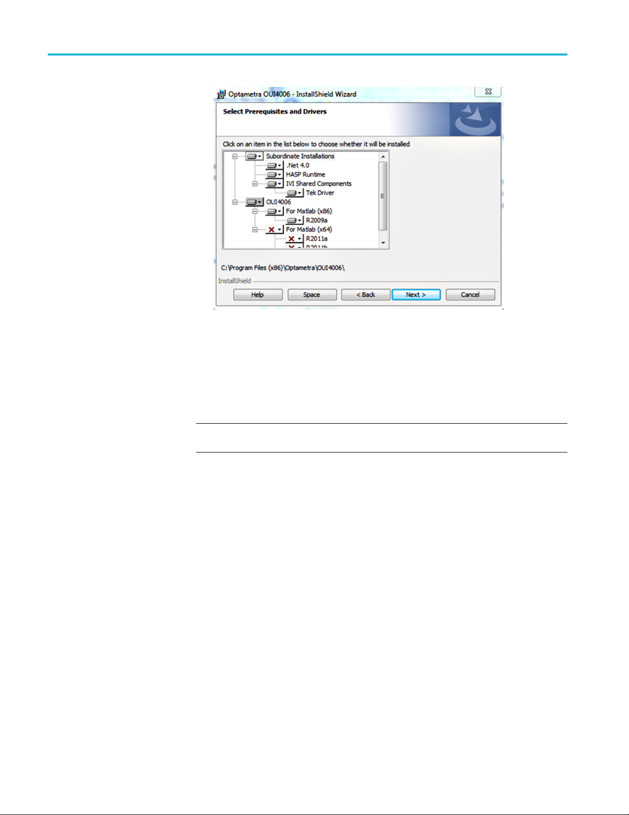
4. Accept the license agreement and select the default options until you get to the choice for Complete or Custom. Select Custom to open the Select Prerequisites and Drivers dialog box.

OM1106 Analysis Software User Manual 5

Install software

5. Examine t the installer has properly identiﬁed the correct MATLAB version to use with the OMA. In the above example, the installer has identiﬁed that MATLAB R2009a is installed and will be used with the OMA.

If there are multiple Matlab versions, use this list to disable all versions of MATLAB except the one that is required for your Windows O S.

NOTE. For future partial updates or re-installs, turn off all of the Subordinate

Installation items except for the ones you are updating.

6. Click Next to begin installation. The Install Wizard launches individual installers as required, such as for the HASP and IVI software.

7. Select Finish when the installer completes successfully.

OMA desktop icons. The install program adds two OMA application icons to

The

the desktop, which start different versions of OMA:

he Select Prerequisites and Drivers installation list to verify that

6 OM1106 Analysis Software User Manual

Install software

Tektronix OUI (xx-bit) - Vertex Processing: This version uses your Graphics Processing Unit (GPU) to add features and enhance performance of the User Interface. The required minimum OpenGL version is 2.1.0 which most recent PCs support. If the graphics driver is out of date, a prom recommended nVidia type, color-grade features will be enabled.

that lack support for Open GL 2.1.0 and for which no driver is available. This version disables some features including 3-D plots, Signal-vs-Time, and color grade options.

To determine if color shading and 3-d plots work on your controller PC, see the verify installation procedure. (See page 10, Verify software installation.)

pt to install latest driver may appear. If the GPU present is the

Tektronix OUI (xx-bit): This version is for older computers

To install Sco pe Service

Utility (SSU) software

The Scope Service Utility (SSU) is required for OMA to communicate with Tektronix MSO/DSO70000C/D/DX/SX series real-time (RT) oscilloscopes and the DSA8300 equivalent-time (ET) oscilloscope. The SSU is installed and runs on the target oscilloscope to collect and send data to the OMA.

There are separate SSU installation programs for RT oscilloscopes and ET oscilloscopes.

To install the SSU:

1. If SSU is installed on the oscilloscope, uninstall the current version before installing the new version.

2. Insert the OMA software media USB drive into a USB p ort on the oscilloscope.

3. Navigate to the appropriate SSU software installation ﬁle (RT or ET) (from

the USB root directory):

For MSO/DSO70000C/D/DX/SX RT oscilloscopes:

OUI\Tektronix Scope Service Utilityx.x.x.x.exe

For the DSA8300 ET oscilloscope:

OUI\Tektronix Scope Service For ET Utilityx.x.x.x.exe

4. Double-click the appropriate program ﬁle to install. Follow any on-screen

instructions. The installer adds SSU icons on the oscilloscope desktop.

Using the SSU. Double-click the Tektronix Scope Service Utility icon to start the SSU software on the oscilloscope before using the OMA to acquire data and analyze results. You can also drag the SSU icon to the Startup folder on real-time

OM1106 Analysis Software User Manual 7

Install software

oscilloscopes the instrument (not available on the DSA8300). The Non-VISA oscilloscope connections (Scope Service Utility) section has more information on SSU. (See page 33, Non-VISA oscilloscope connections (Scope Service Utility).)

NOTE. For ET SSU: Make sure that the oscilloscope application AND the Socket

Server are running before running the ET Scope Service Utility. To start the socket server, rig

ET SSU operation. The ﬁrst time you run the SSU program on the ET oscilloscope, it will as E: DSA8300 equivalent-time (ET) oscilloscope operation. Once you do this and click OK, the default state is saved to My Documents\TekScope\UI\default.st.

This default ﬁle loads each time you start the Scope Service Utility to recall the deskew and other important settings. You can change the default state at any time by saving over the de fault state ﬁle.

To verify equivalent-time function of the OMA, load a simulated ET ﬁle and display the results:

1. Check that the OMA Matlab Engine Command Window contains the line CoreProcessingCommands (this is used instead of CoreProcessing to enable

either ET o

so that the SSU starts automatically when you power-on or reboot

ht click the network icon on the oscilloscope.

k you to set up the oscilloscope according to the instructions in Appendix

r RT processing of the data).

2. Click Home > 1-pol I&Q.

3. Click Ofﬂine > Load and navigate to and select the ﬁle My Documents\Tek Applications\OUI\MAT Files\Simulated ET Data Files\QPSK2chAET.mat.

4. Click the Run-

shown in the following image (after using the plot scaling controls, marked in red, to reduce the plot sizes):

Stop button in the Ofﬂine Commands area. A successful run is

8 OM1106 Analysis Software User Manual

Install software

Updating exis

ting OMA (OUI) installations

Do the following before replacing an earlier version of OMA (referred to as OUI in earlier releases):

Back up any critical data ﬁles; in particular, back up pHybCalib.mat and EqFiltCoef.mat from the C:\Program Files\TekApplications\OUI\ folder, and replace the

Back up any ﬁles you may have edited in the \Program Files\Optametra folder or \Progra

Record your channel delay values on the Calibration tab. If upgrading from an older OUI Starting with OUI V1.6, the top slider is the Channel XI to XQ delay, the middle slider is Channel XI to YI and the bottom is now Channel YI to YQ.

If you have the XI to YQ value but not the YI to YQ value, simply subtract the XI to YI value from the XI to YQ value to get the YI to YQ value.

NOTE. Please call Tektronix for assistance if upgrading from OUI V1.4 or V1.5

that is installed on an oscilloscope.

Do the following to upgrade from OUI4006 Version 1.3 or earlier to the current software, when installed on a PC (not an oscilloscope). Using the Remove Program tool in the system Control Panel to:

m in the new ExecFiles folder after the upgrade is complete.

m Files\TekApplications sub folders.

version, the format of the Channel Delay sliders may be different.

Uninstall the Scope speciﬁc IVI driver (for example, TekScope IVI Driver

2.7).

Uninstall the IVI Shared Components (do NOT uninstall the VISA Shared

Components).

Uninstall OUI4006 (version 1.3 or earlier).

Uninstall LRCP (if present) by using the remove program feature in the

system Control Panel.

Install this version of OMA and required softwa re.

If the OUI installer asks to uninstall an old HASP driver and install a new one, click YES. This p revents future problems with Windows Updates.

OM1106 Analysis Software User Manual 9

Install software

Verify softwa

re installation

Do the following to verify that OMA and MATLAB are installed correctly:

1. Insert the product USB HASP key in a USB port on the controller PC.

3. Click the Home menu tab, and then click the 1-pol I&Q button (in the Layout

4. Right-c

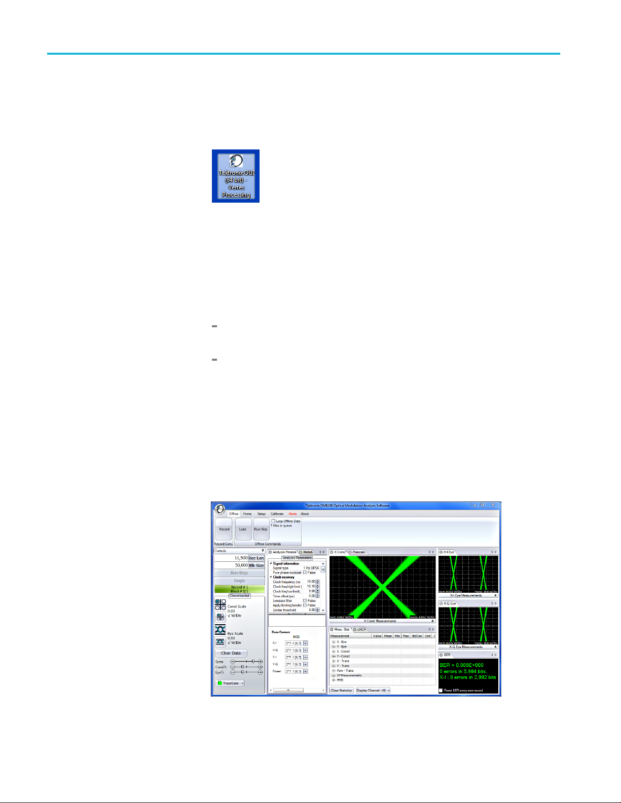
Double-click the desktop OMA icon Tektronix OUI (xx bit)

Vertex Processing. Wait for the OMA application to open. If the OMA

application opens but seems to be locked up, see the troubleshooting s ection. (See page 11,

section o readout, and control tabs for the 1-pol I&Q measurement.

If the Color Grade menu item is selectable, then the graphics card on your

contro

If the Color Grade menu item is grayed out, then the graphics card on your

contr Close OMA and then restart OMA using the Tektronix OUI (xx bit) desktop icon. Then repeat this procedure and continue to the next step.

Troubleshooting OMA/MATLAB installation.)

f the menu bar). The OMA screen populates to show the plot,

lickintheX-I Eye plot to open the X-I Eye Options context menu:

ller PC supports color grade and 3-d plots.

oller PC does not support the Vertex Processing version of OMA.

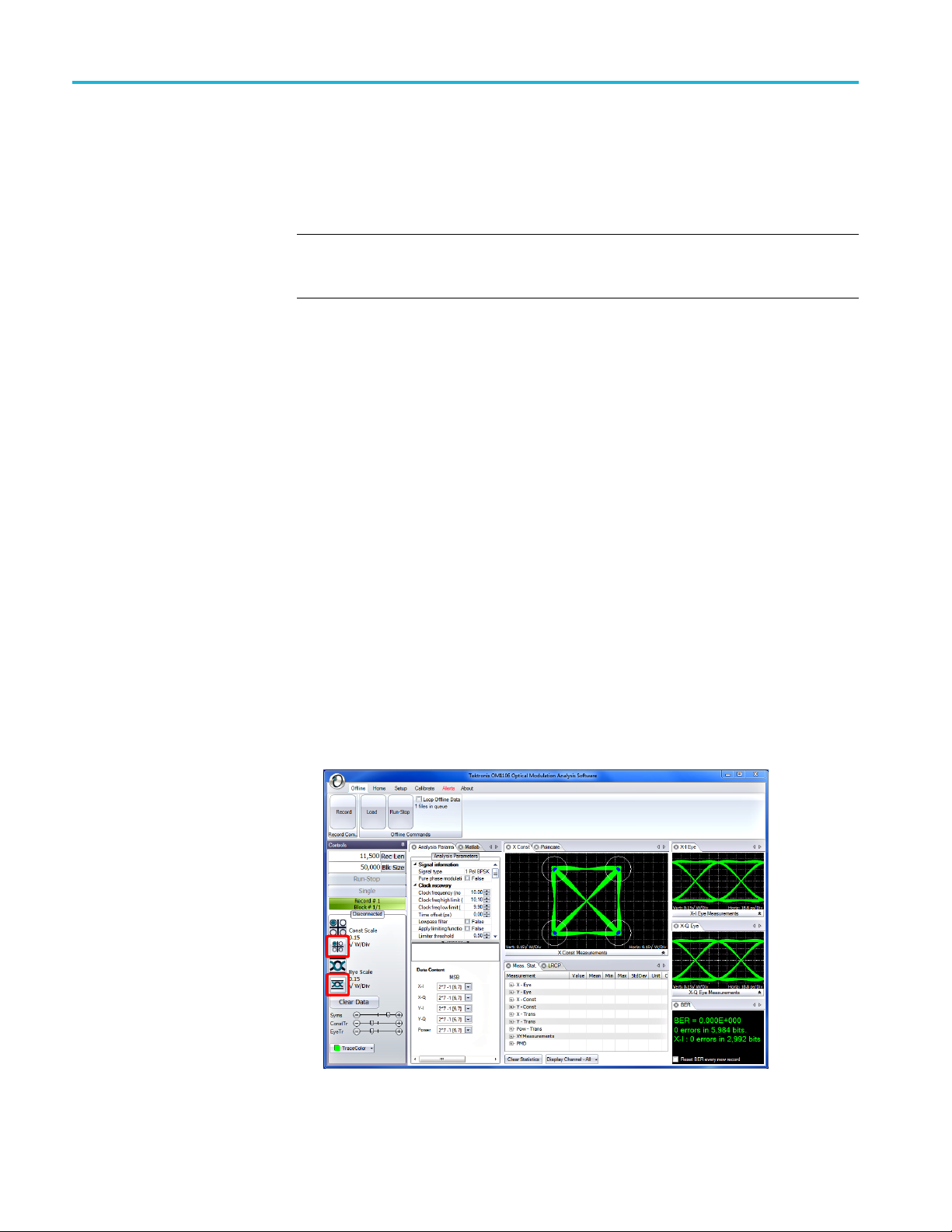
5. Click Ofﬂine in the menu bar, click Load, and navigate to My Documents\TekApplications\OUI\Mat Files\Simulated Data Files.

6. Select ﬁle QPSK1chA.mat. and click Open.

ick Run-Stop (in the Ofﬂine menu bar). The OMA screen should look

7. Cl

similar to the following image:

10 OM1106 Analysis Software User Manual

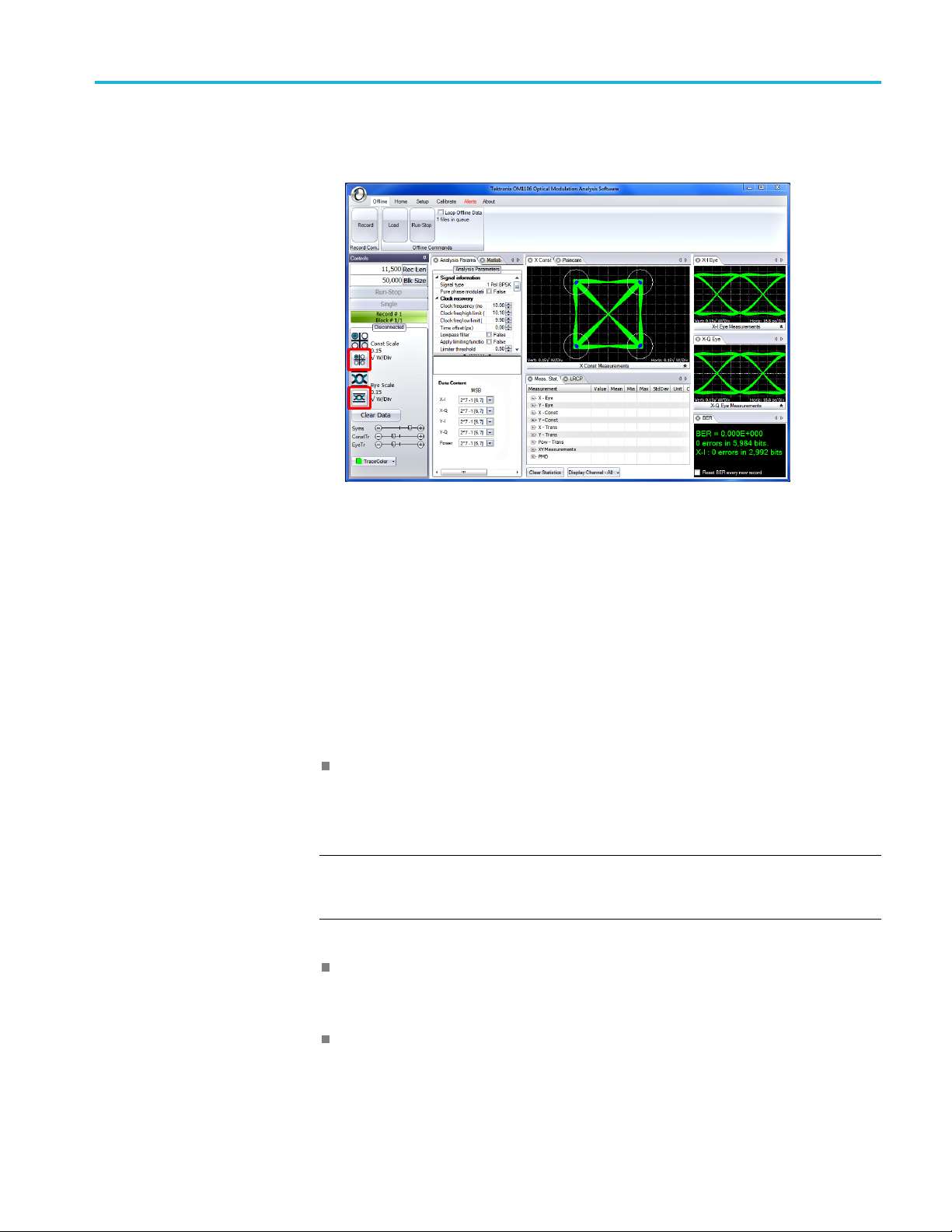
Install software

8. Click the Cont S image) to reduce the plot scales to show the entire plot.

9. If you see the above screen, then OMA and MATLAB installed correctly.

Go to the Verify or set OM series instrument IP address section to set OM instrument connections. (See page 13.)

cale and Eye Scale buttons (marked in red on the following

Further information

Troubleshooting

OMA/M

ATLAB installation

Go to the Scope Connect section to learn how to connect to an oscilloscope. (See page 29, Scope Connect button.)

If the OMA window opens, but is not functional (appears to lock up), the most

ly cause is a MATLAB version or activation problem.

Open the MATLAB software interface and check that the correct version was

talled. If the wrong version of MATLAB was installed, uninstall both

ins MATLAB and OMA, and then reinstall the software following the installation order and instructions in this manual.

TE. If more than one MATLAB version is installed on the controller PC, OMA

may be ‘connected’ to the wrong version. (See page 12, Using other MATLAB installations.)

f the version is correct, conﬁrm that the MATLAB software was successfully

I activated after the install (see the MATLAB install instructions for h ow to activate the program).

If the above items do not ﬁx the problem, please contact Tektronix Customer Support for assistance.

OM1106 Analysis Software User Manual 11

Install software

Using other MATLAB

installations

Unexpected results

Verify HASP protection

Reverting to ot multiple MATLAB installation: To use a version of MATLAB that is not the most recent one installed on your computer, you need to register the older version as the COM server. This is done as follows:

Once MATLAB installation completes, ﬁnd the shortcut for the MATLAB version you want to use and double click it to start the MATLAB Desktop for that version.

Run the following two lines in the MATLAB Command window to establish the running Matlab.exe as the correct Com-Server: cd(fullﬁle(matlabroot,'bin',computer('arch'))) !matlab /

If you get unexpected results, note a nything reported in the MATLAB Engine Response Window, or in the Alerts tab. Also open the MATLAB Comman CoreProcessingCommands, and note any response. Provide this information when contacting Tektronix Customer Service.

You c a Control Center:

n verify the HASP protection b y opening the SafeNet Sentinel Admin

her MATLAB versions or post installation steps for a system with

regserver

d Window from the MATLAB desktop application, enter

1. Open

2. Cli

3. Verify that your key is listed as a local HASP HL Pro key.

a web browser on the controller PC and enter http://localhost:1947 in

the address bar to open the Sentinel Admin Control Center Web page.

ck the Sentinel Keys link in the left panel.

12 OM1106 Analysis Software User Manual

Verify or set OM series instrument IP address

Verify or set O

Verify OM

instrument connectivity on DHCP-enabled network

M series instrument IP address

Before you ca that IP addresses of the connected OM series instruments are set correctly for your network, to enable communications between the instruments and the OMA software. The following sections describe how to connect OM instruments to DHCP and non-DHCP networks.

All OM instruments must be set to the same network subnet (DHCP-enabled networks do this automatically) to communicate with each other.

OM series instruments are set by default to use DHCP to automatically assign IP addresses. If you are connecting the OM instruments and PC controller over a DHCP net as the DHCP server automatically assigns an IP address during each instrument’s power-on process.

The following procedure describes how to verify that the OMA software can detect and connect to OM instruments that are set to use DHCP-generated IP addresses on a DHCP-enabled network:

n use the OMA software to take measurements, you must make sure

work, you do not need to speciﬁcally set the OM instrument IP address,

Verify OMA can detect

M instruments on DHCP

network

Prerequisites:

Required software is installed on the controller PC (OMA, MATLAB, and so on).

OM instrument(s) and the controller PC are connected to the same DHCP-enabled local network.

OM instruments are set to use DHCP (default conﬁguration).

To verify that the OMA software can detect and connect to OM instruments

ocated on a DHCP-enabled local network:

1. Connect the OM instrument(s) to the D HCP-enabled local network.

2. Power on each OM instrument. The instrument queries the DHCP server

to obtain an IP address. Wait until the front panel Enable/Standby button light turns off, indicating it has obtained an address. Push the front panel Enable/Standby button to enable the network connection (button light turns On).

3. Double-click the Tektronix OUI software desktop icon to start the OMA software.

4. Click Setup > Optical Connect to open the Device Setup dialog box.

OM1106 Analysis Software User Manual 13

Verify or set OM series instrument IP address

5. Click Auto Con ﬁ instruments. If all connected instruments are listed, then correct IP addresses were automatically assigned.

If the Device Setup dialog does not list all connected instruments:

Verify that

network.

Verify that

for network access (front panel power button light is on).

Work wit h y

6. Click OK to close the Device Setup dialog box and return to the OMA main screen. T

he OMA software can now access and control the OM instruments.

gure to search the network and list all detected OM

instruments are connected to the correct DHCP-enabled

instruments are powered on and in the correct power-on state

our IT resource to resolve the connection problem.

Set OM instrument IP address for use on non-DHCP network

To conn IP address and related settings on the OM instrument to match those of your non-DHCP network. All devices on non-DHCP network (OM instruments, PCs running OM software, and other remotely accessed instruments such as oscilloscopes) need the same subnet values (ﬁrst three number groups of the IP address) to communicate, and a unique instrument identiﬁer (the fourth number grou

ect the OM series instrument to a non-DHCP network, you must set the

p of the IP address) to identify each instrument.

Work with your network administrator to obtain a unique IP address for each

ice. If your network administrator needs the MAC address of the OM

dev instrument, the MAC address is located on the instrument rear panel label.

NOTE. Make sure to record the IP addresses used for each OM instrument, or

attach a label with the new IP address to the instrument.

If you are setting up a new isolated network just for controlling OM and associated

nstruments, Tektronix recommends using the OM instrument default IP subnet

i address of 172.17.200.XXX, where XXX is any number between 0 and 255.

NOTE. Use the system conﬁguration tools on the oscilloscope and computer to

set their IP addresses.

NOTE. If you need to change the default IP address of more than one OM

instrument, you must connect each instrument separately to change the IP address.

14 OM1106 Analysis Software User Manual

Verify or set OM series instrument IP address

Change OM instrument

IP address using DHCP

network

There are two wa

Connect the OM instrument(s) to a DHCP-enabled network and use the LRCP tab in OMA to change the IP address (easiest way).

Connect t already set to the same IP address subnet as the OM instrument, and use the LRCP tab controls in OMA to change the IP address.

To use a DHCP network to c hange the IP address of an OM instrument:

1. Connect the OM instrument(s) to the DHCP-enabled network.

2. Power on the OM instrument. The instrument qu

3. Access the connection setup controls:

OM1106:

a. Double-click the OM1106 software desktop icon.

b. Click Setup > Optical Connect to open the Device Setup dialog box.

ys to change the IP address of an OM instrument:

he OM instrument directly to a PC (with OMA installed) that is

eries the DHCP server

LRCP:

Double-click the LRCP desktop icon. Enter password 1234 if

requested.

Click Device Setup to open the Device Setup dialog box.

4. Click Auto Conﬁgure to search the network and list all detected OM instruments.

If the Device Setup dialog does not list all connected instruments:

Verify that instruments are connected to the correct DHCP-enabled

network

Verify that instruments are powered on

Work with your IT resource to resolve the connection problem

5. Double-click in the IP Address ﬁeld of the instrument to change and enter the new IP address for that OM instrument.

6. Click the corresponding Set IP button. A warning dialog box appears indicating that the IP address will be changed and that you must record the new IP address. Losing the IP address will require connecting the instrument to a DHCP router.

7. Click Ye s to set the new IP address.

OM1106 Analysis Software User Manual 15

Verify or set OM series instrument IP address

Change OM instrument IP

address using direct PC

connection

8. Edit the Gatewa support).

9. Click OK.

10. Repeat steps 5 through 9 to change any other OM instrument IP addresses.

11. Exit the OM program.

12. Power off the OM instrument(s) and connect it to the non-DHCP network.

13. Run LRCP or OM1106 on the non-DHCP netwo

button in the Device Setup dialog box to verify that the instrument is listed with the new IP address.

To use a direct PC connection to change the default IP address of an OM instrument, you need to:

Install OM1106 or LRCP on the PC

UsetheWindowsNetworktoolstosettheIPaddressofthePCtomatchthat of the current subnet setting of the OM series instrument whose IP address youneedtochange

Connect the OM instrument directly to the PC, or through a hub or switch (not over a network)

y and Net Mask (obtain this information from your network

rk and use the Auto Conﬁg

Use OM1106 or LRCP to change the OM instrument IP address

Do the following steps to use a direct PC connection to change the IP address of an OM series instrument:

NOTE. The following instructions are for Windows 7.

NOTE. If you need to change the default IP address of more than one OM

instrument using this procedure, you must connect each instrument se change the IP address.

Set PC IP address to match OM instrument.

1. On the PC with OM1106 or LRCP installed, click Start > Control Panel.

2. Open the Network a nd Sharing Center link.

3. Click the Manage Network Connections link to list c onnections for your PC

4. Right-click the Local Area Connection entry for the Ethernet connection and select Properties to open the Properties dialog box.

5. Select Internet Protocol Version 4 and click Properties.

parately to

16 OM1106 Analysis Software User Manual

Verify or set OM series instrument IP address

6. Enter a new IP ad used by the OM instrument. For example, 172.17.200.200. This sets your PC to the same subnet (ﬁrst three number groups) as the default IP address setting for the OM series instruments.

7. Click OK to set the new IP address.

8. Click OK to exit the Local Area Connection dialog box.

9. Exit the Control Panel window.

Run OMA on direct-connected PC to change OM instrument IP address.

1. Connect the OM instrument to the PC (directly, or through a hub or switch connected to the PC). Do not connect over a network.

2. Power on the OM instrument. Wait until the front panel Enable/Standby button light turns Off.

3. Push the Enable/Standby button again to enable the network connection (button light turns On).

4. Double-click the OM1106 software desktop icon.

5. Click Setup > Optical Connect to open the Device Setup dialog box.

6. Click Auto Conﬁgure to search the network and list all detected OM

instruments.

dress for your PC, using the same ﬁrst three numbers as

If the Device Setup dialog does not list all connected instruments:

Verify that instruments are connected to the correct DHCP-enabled

network

Verify that instruments are powered on

Work with your IT resource to resolve the connection pr

7. Double-click in the IP Address ﬁeld of the instrument to change and enter the new IP address for that OM instrument.

8. Click the corresponding Set IP button. A warning dialog box appears indicating that the IP address will be changed and that you must record the new IP address. Losing the IP address will require connecting the instrument to a DHCP router.

9. Click Ye s to set the new IP address.

10. Edit the Gateway and Net Mask (obtain this information from your network

support).

11. Click OK.

12. Exit the OM program.

13. Power off the OM instrument.

oblem

OM1106 Analysis Software User Manual 17

Verify or set OM series instrument IP address

14. Disconnect the

15. Connect the OM instrument to the target network.

16. Run the OM1106 or LRCP software on the PC connected to the same

network as the OM instrument to verify that the OM software detects the OM instrume

OM instrument from the PC.

nt.

18 OM1106 Analysis Software User Manual

OM1106 Optical Modulation Analysis (OMA) user interface

The OM1106 Optical Modulation Analysis Software user interface (referred to as the OMA or OMA software throughout this document) is a powerful and ﬂexible pane of OMA are:

l-based user interface for optical signal analysis. The main functions

Detect OM in

Set parameters on the OM instruments (laser, modulator, and so on)

Provide communication between all detected OM instruments, oscilloscopes, and the OMA software

Acquire and process signals from OM instruments and the oscilloscope

Display plots and measurements

struments on the local network.

Figure 1: The OMA screen with plots and measurements

OM1106 Analysis Software User Manual 19

OM1106 Optical Modulation Analysis (OMA) user interface

To sta rt the OMA screen.

NOTE. Inser

the OMA.

t the application HASP key into a USB port on the PC before starting

software, double-click the desktop icon to open the default

The OM be installed on the same PC as the OMA sofware. The OMA automatically launches and interfaces with the MATLAB application using engine mode. No direct user interaction with MATLAB is needed for most operations while using the OMA.

NOTE. MATLAB must be installed and activated before running the OMA

sof

NOTE. Typin g desktop in the separate Matlab application window opens the

A requires a third party program, MATLAB by MathWorks, which must

tware.

ll Matlab UI.

20 OM1106 Analysis Software User Manual

OM1106 Optical Modulation Analysis (OMA) user interface

OMA user inter

face elements

The Menu ribbon

Figure 2: Default OMA startup screen

Item Description

The Menu ribbon provides fast access to key tasks. Click a main menu tab to show the associated task buttons.

Clickanicontoshowthemenuofavailable functions and sub-functions, open a dialog box, or run that task.

The Menu ribbon provides fast access to key tasks.

The Plots panel is a ﬂexible panel-based area that displays the plots, measurement, and parameter control panels. (See page 22.)

The global Controls panel sets record length and block size, runs and stops live data acquisitions, sets plot display scales, and shows other controls as needed for particular plots. (See page 28.)

OM1106 Analysis Software User Manual 21

OM1106 Optical Modulation Analysis (OMA) user interface

The menu ribbon buttons can be hidden to provide more room for plots and control tabs. To hide the menu bar, double click any main menu tab other than About. Unhi

de by double clicking again on a tab.

The Plots panel

The Plots and parameter control panels. The Plots panel is empty by default when you start OMA. Select a predeﬁned plot layout from the Home > Layout buttons to quickly populate the plot panel with parameter, control, and plots for the selected measurement. The following image shows the Plots panel populated by selecting the 2-pol I&Q layout button.

panel is a ﬂexible panel-based area that displays the plots, measurement,

Select individual plots and measurements from the Home menu items to add to the Plots panel. New individually added plots open as full-screen plot on blank screens, or are added to an existing a rea when inserted in an existing layout, with each plot, readout, or control on its own tab. You can move plot, control, and readout tabs (referred to a s plots throughout this manual) within the Plots panel area or drag them to the PC desktop.

22 OM1106 Analysis Software User Manual

OM1106 Optical Modulation Analysis (OMA) user interface

To change plot tab order. To change the plot tab order (within the same group of plot tab

To move/arrange plots in the Plots panel. To move and arrange plots within the Plots panel, click and drag a plot tab into any open plot. OMA shows a plot position icon. Continue holding the mouse button and drag the cursor on to the positioning guide.

s), click and hold on the tab and drag it horizontally in the same tab group.

s you drag the cursor on the different areas of the plot position icon, the screen

A is shaded light blue to indicate where the plot will be positioned (above, below, left, or right of the current plot).

OM1106 Analysis Software User Manual 23

OM1106 Optical Modulation Analysis (OMA) user interface

Release the mouse button and the OMA places the plot into a new panel in the selected area.

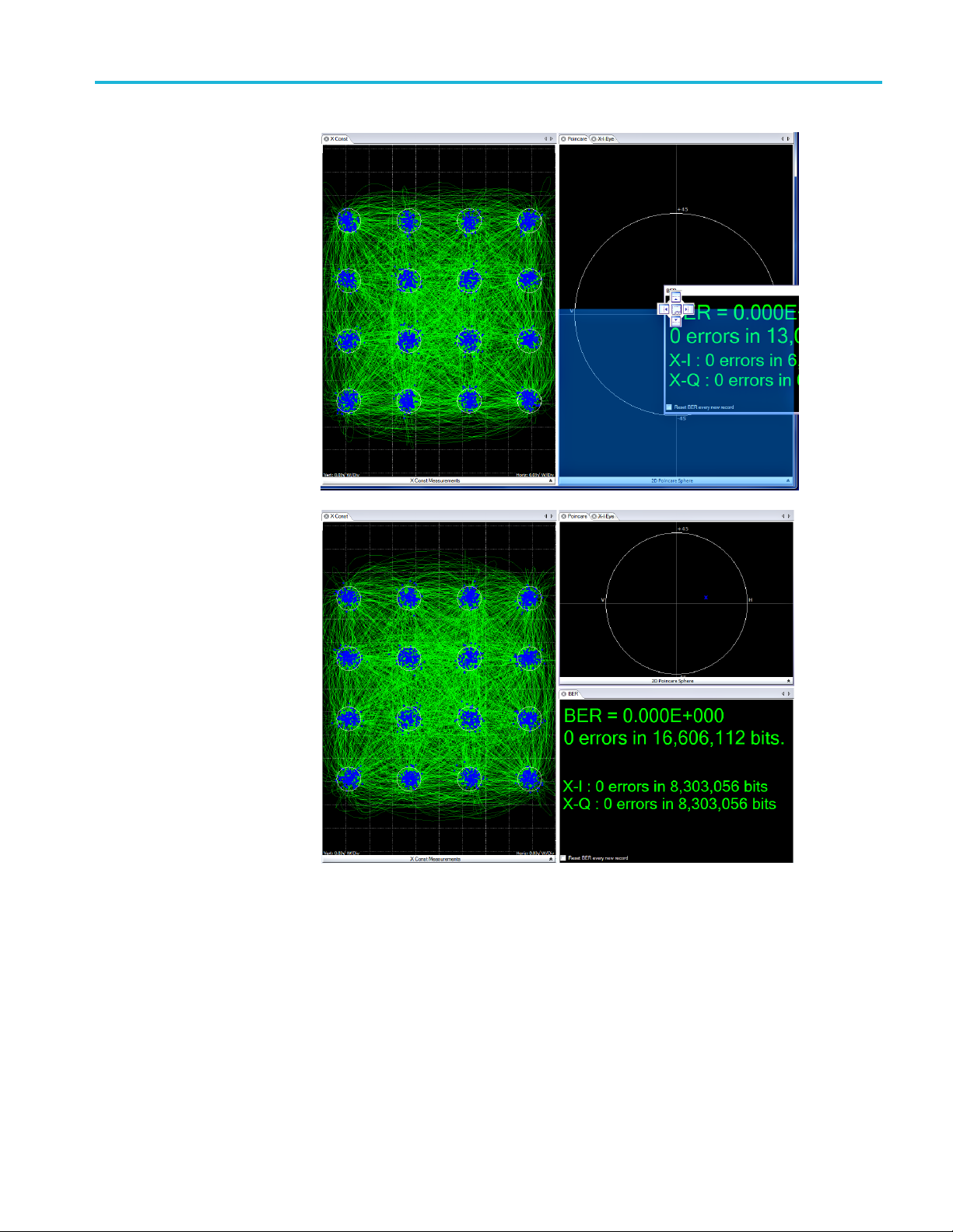
The following images show moving the BER plot to display below the Poincaré plot, and the X-I Eye plot to display below the constellation plot.

24 OM1106 Analysis Software User Manual

OM1106 Optical Modulation Analysis (OMA) user interface

OM1106 Analysis Software User Manual 25

OM1106 Optical Modulation Analysis (OMA) user interface

Dragging a plot to the center of the positioning icon places the m oved plot as a tab in the plot pane to which it was dragged.

To move a

desktop, click and hold on the plot tab and drag it to the desktop. To return the plot to the OMA application, double click in the title bar of the desktop plot window.

NOTE. The plot may not move back to the same position in the Plots panel from

whereyourdraggedit.

plot to the desktop. To move a plot to a separate window on the

26 OM1106 Analysis Software User Manual

OM1106 Optical Modulation Analysis (OMA) user interface

To save p

using the Load Preset and Save Preset functions in the Home ribbon menu. (See page 106, Layout controls.)

To show additional plot controls, information. Plots may have dropdown panels to show extra information or controls associated with that plot. Click the double

arrow on the bottom border of a tab for that tab.

To re

area between plots; the cursor changes shape to a bar with arrows. Click and hold the right mouse button and drag the panel divider to change the panel size.

To delete a plot. To delete a plot, click the X icon (circled in red in the following image).

To show additional plot display settings. Plots may have additional display settings (markers, save to, color grade, trace color, and so on). Right-click in a plot to see available display or other options.

lot layouts. You can save and recall (load) custom plot layouts by

to display or hide the extra information

size plot panels. To resize a plot panel, position the cursor in the g ray d ivider

OM1106 Analysis Software User Manual 27

OM1106 Optical Modulation Analysis (OMA) user interface

The global Con

trols panel

The global Controls panel sets record length and block size, runs and stops live data acq particular plots. This control panel is pinned to the left side of the application by default for easy access. You can click the pushpin icon in the upper right to minimize the controls to allow for maximum Plot panel area.

uisitions, sets plot display scales, and shows other controls as needed for

You can rescale Constellation and Eye plots by clicking on the relevant Plot icons in the Controls panel (located by default on the left side of the application). The scale units are √W/div.

There are also controls to adjust the intensity of symbol points and the intensity and color of constellation and eye traces. You can also adjust trace color and intensity levels may using the right-click menu on each individual plot. (See

e115,The global Controls panel.)

pag

28 OM1106 Analysis Software User Manual

The Setup tab controls

Use the Setup tab controls to detect, connect, and conﬁgure connected oscilloscopes (real-time and equivalent time) and OM series instruments to perform meas the controls in detail, grouped by the control categories (Scope Setup, Optical Setup, Reference Laser, Show Controls, and State Control).

Scope Setup controls

Scope Connect button

The Scope Connect functions search for and connect to network-connected oscilloscopes, and assign oscilloscope channels to the OM instrument inputs. Click Scope Connect on the Setup tab to open the ScopeConnectionDialog box.

urements with the OMA software. The following sections describe

NOTE. The Scope Connect functions require that the Scope Service Utility (SSU)

stalled and running on connected oscilloscopes.

be in

OM1106 Analysis Software User Manual 29

Scope Setup controls

A green progres oscilloscopes on the same subnet that are running the Scope Service Utility (SSU). As they are found they are added to the drop-down menu. Click the IP address ﬁeld and select the IP of the oscilloscope to which to connect, then click Connect.

If the OMA Scope Connection Dialog box reports 0 Scopes Found, you will have to manually enter the IP address. This happens when connecting over a VPN or when network policies prevent the IP broadcast. When typing the address in manually, do not include “, ET” or “, RT” on the end; just enter the IP address. Click Conn

After connection, use the Scope Data Setup ﬁelds to map the oscilloscope channels to the OM i ﬁelds. The MATLAB variable storing the oscilloscope data is named Vblock. Data from the selected channel is moved into the indicated Vblock variable.

Vblock(1) – X-polarization, In-Phase

Vblock

Vblock(3) – Y-polarization, In-Phase

Vblock(4) – Y-polarization, Quadrature

s bar at the top indicates that the software is searching for

ect.

nstrument receiver channels and corresponding MATLAB variable

(2) – X-polarization, Quadrature

There are two features which may be enabled on this di alog box . "Enable auto setup on connection" means that any time you connect to an oscilloscope, the oscilloscope will be requested to restore the state saved the last time the OUI was closed.

"Enable auto connection on program launch" means the oscillosc ope connection will be made automatically when the OUI software is launched. This assumes that the oscilloscope is present at the last IP address where it was found and that the Scope Service Utility is running on the oscilloscope. It is a good idea to use ﬁxed or reserved IP addresses when using any autoconnect features.

30 OM1106 Analysis Software User Manual

Scope Setup controls

Once connected

Click Enable Slave Connection to enable selecting a second IP address. Find the two oscillosc the one receiving the external trigger. The Slave oscilloscope is the one triggering on the sync board output only. (See page 167, Conﬁguring two Tektronix 70000 series oscilloscopes.)

NOTE. The DPO/DPS70000SX series oscilloscopes behave as a single

oscilloscope when connected in the UltraSync conﬁguration, and do not require the second

Use VISA control (Scope Setup)

Click (select) the Use VISA box in the Scope Setup area of the Setup menu to use TekV series oscilloscope.

NOTE. Click Use VISA before clicking Scope Connect.

NOTE. Do not select the “Use VISA” box when connecting to Tektronix DSA8300

equivalent time (ET) sampling o scilloscope or MSO/DSO70000C/D/DX/SX series real-time (RT) oscilloscopes.

ISA to communicate with a Tektronix MSO/DSO70000 or 70000B

and conﬁgured, close the connect dialog box.

opes and decide which one is the Master. The Master oscilloscope is

IP address.

Click the Connect button to open the VISA-speciﬁc Scope Connection Dialog box.

OM1106 Analysis Software User Manual 31

Scope Setup controls

VISA connections

The VISA addres from the previous session, so it should not normally need to be changed, unless the network or the oscilloscope has changed. The VISA address string should be TCPIP0::IPADDRESS::INSTR where IPADDRESS is replaced by the oscilloscope IP address, for example 172.17.200.138 in the example below.

NOTE. To quickly determine the oscilloscope IP address, open a command

window (“DO instrument IP address.

After clicking Connect, the drop down boxes are populated for channel conﬁguration. Choose the oscilloscope channel name which corresponds to each receiver output and MATLAB variable name. These are:

Vblock(1) – X-polarization, In-Phase

Vblock(2) – X-polarization, Quadrature

Vblock(3) – Y-polarization, In-Phase

Vblock(4) – Y-polarization, Quadrature

llowing example disables two channels and sets the other two channels to

The fo Channel 1 and Channel 3, since these can be active channels in 100Gs/s mode. The disabled channels must still have some sort of valid drop-down box choice. Do not leave the choice blank.

s of the oscilloscope contains its IP address, which is retained

S box”) on the oscilloscope and enter ipconﬁg/allto display the

NOTE. It is important to have the oscilloscope in single-acquisition mode (not Run

mode). If you put the oscilloscope into Run mode to make some adjustment, please

ember to click Single on the oscilloscope before connecting from the OMA.

rem

32 OM1106 Analysis Software User Manual

Scope Setup controls

Table 1: Oscill

OMA Capabilit

Segmented re

Ability to c oscilloscopes running the Scope Service

Scope conﬁg, Auto connect, Auto scale, and Deskew

Software required on oscilloscope

DPO/DPS 7

Real-time oscilloscope compatibility Any real-time

lent-time oscillos cope compatibility

Equiva

oscope connectivity capabilities (TekVISA vs. Scope Service Utility)

adout for unlimited record size

ollect data from two networked

0000 SX series compatibility

TekVISA

Yes Yes

No Yes

LAN server

No Yes

Tektr on oscilloscope supported by the

IVI driv

Scope Service U tility (non-TekVISA

RT or ET Scope Service U

MSO/DSO D, DX, SX series oscilloscopes with ﬁrmware later

DSA8300 with ET Scope Service

Utilit

)

tility

70000C,

v6.4 or

Non-VISA oscilloscope

connections (Scope

Service Utility)

As men

tioned above, the other choice for connecting to the oscilloscope and collecting data is through the Scope Service Utility (SSU). The SSU is a program that runs on each oscilloscope c onnected to the OMA controller PC.

NOTE. The Scope Service Utility runs on the target oscilloscope. Be sure to

install the proper version of SSU for either real-time or equivalent-time (ET) oscilloscopes. See installation guide.

ce the SSU is installed on the oscilloscope, start the “Socket Server” and the

On TekScope oscilloscope application, then double-click the SSU desktop icon to start the SSU application. Minimize the application before connecting to the oscilloscope from OMA.

NOTE. It is best to set the oscilloscope to single-acquisition mode (not Run mode).

The Scope Service Utility takes data directly from the oscilloscope memory and sends it over a WCF interface to the OMA.

OM1106 Analysis Software User Manual 33

Scope Setup controls

Auto Scal

When connectin check the box unless you require a VISA connection.

NOTE. Clicking Connect on the OMA Setup Tab opens the Scope Connection

dialog box for connecting to the SSU. (See page 29, Scope Connect button.)

Once the oscilloscope connection is conﬁgured, close the Connect dialog box. Then use the Conﬁgure Scope, Auto Scale, and Scope & Receiver Deskew buttons (in that order) to ﬁnish setting up oscilloscope.

e and DC Calib button

Click the Auto Scale and DC Calib button once you have connected to an oscilloscope and have prepared your signal and Reference laser as required for your tes may have changed.

DC Cali anytime the an Auto Scale is requested. To run DC Calibration without an Auto Scale, use the button on the Calibration tab.

ting. Click Auto Scale any time the signal level from the oscilloscope

bration (measuring and removing static dc offsets) will be performed

g from the OMA, you will see a check box for VISA. Do not

Auto Scale senses the size of the signal on each oscilloscope input to determine the proper scale and offset settings, and then sets the o scilloscope with the settings.

Scope & Receiver Deskew button

Click the Scope & Receiver Deskew button to open the tool dialog box.

34 OM1106 Analysis Software User Manual

Scope Setup controls

The Scope & Rece new OMA setup or one that has had any changes to the X, Y, I, or Q path lengths or cabling. The dialog box includes instructions on how to set up for deskewing.

Select the Skew measurement range. The range should be between 25% and 50% of the combined OMA/oscilloscope sys tem bandwidth. The default value of 10 GHz works in most cases.

The laser grid is changed for this measurement because it may be necessary to tune continuously across grid points. If you are already using a 10 or 12.5 GHz grid, choose that value for the grid to be used for the deskew. If you are using a different grid, the grid is set back to its original value after the deskew is complete time or decreased to collect more data.

Select t original wavelength after the deskew. Skew is a not a signiﬁcant function of wavelength, so the test wavelength can be chosen to be any convenient value inside of the tuning range of the Signal and Reference lasers.

Set the minimum expected system bandwidth to be equal to the lesser of the OMA and oscilloscope bandwidths. The deskew utility will report an error if no signal is found at any frequency below this v alue. The default value works in most cases.

Once setup is complete and the readiness checks are passed, click Start Deskew to perform the deskew process.

. A step size of 500 MHz is recommended but can be increased to save

he desired test wavelength for the deskew. The lasers are set back to their

iver Deskew dialog box facilitates the deskew process for a

The signal and reference lasers are ﬁne tuned over the speciﬁed skew mea surement range to measure the average phase slope and calculate the relative path delays (skews).

When the deskew process is complete, the values in the Calibration tab "Sliders" area are updated to those measured.

It is a good idea to save the OMA state after completing a deskew to save the values. (see Setup: Save State)

OM1106 Analysis Software User Manual 35

Optical Connect

Optical Conne

The Optical C dialog box, which detects and connects to all OM instruments that it detects on the local network.

Run the Setup > Optical Connect task when you run the OMA software for the ﬁrst time, and any time that you add or remove instruments from the network.

To have OMA detect network-connected instruments:

1. Start OM

2. Click SETUP > Optical Connect to open the Device Setup dialog box.

3. Click Auto Con ﬁgure to search the network and list all detected OM

instruments. This search can take a few minutes.

If the Device Setup dialog does not list all connected instruments:

onnect button (Setup > Optical Connect) opens the Device Setup

Verify that OM instruments are connectedtothecorrectnetwork

Verify that instruments are powered on and their network connection is

enabled (the On/ Standby button on the front panel is on )

NOTE. If it is necessary to reset the instrument network connection, press

and hold the front-panel On/Standby button until the light changes color to

boot the instrument.

If the above items do not help, work with your IT resource to resolve the

connection problem

4. Use the Friendly Name ﬁeld to attach custom labels to OM instruments that help you identify the type and/or location of the instruments. Friendly Names are retained in the LRCP software and are tied to the corresponding instrument MAC address.

5. (Optional) You can use the Set IP button to manually set the instrument IP address. This is only necessary in a network environment that is not using DHCP to automatically assign IP Addresses. (See page 13, Verify or set OM series instrument IP address.) The Set IP button only changes the IP address and does not save other modiﬁed ﬁelds like Friendly Name.

36 OM1106 Analysis Software User Manual

Optical Connect

6. (Optional) Sel this hardware when the OUI/LRCP is launched. The Auto Start hardware is conﬁgured at OUI/LRCP launch to match the state when the OUI/LRCP was last closed. The hardware must be present at the last known IP address for the automatic connection to work.

7. Click OK to exit the dialog and save any changes (such as Friendly Name). OMA lists the detected OM devices as tabs on the main screen, using the friendly name and IP address to allow for easy identiﬁcation.

NOTE. If yo

or saved in the software.

NOTE. OM

Disconnected or powered-off instruments will still be shown in the list and be shown as ofﬂine. You should run the Auto Conﬁgure task in on a regular basis after starting OMA or if OMA has been on for a long period of time, to update the connected device list.

A does not automatically update the connected devices list on startup.

ect Auto Start to enable auto connection and conﬁguration of

u do not click OK, the listed instruments are not connected to LRCP

OM1106 Analysis Software User Manual 37

Optical Control Panel (LRCP)

Optical Contr

ol Panel (LRCP)

Click the Opt tab in the Plots panel. The LRCP lets you control connected instrument lasers and modulator par ameters.

LRCP creates a tab for each detected instrument, labeled with the device n ame and IP address. Clicking an instrument tab displays the available controls for that device. The contents of a control pane depend on the O M instrument associated with that tab.

ical Setup button to open a LRCP (Laser/Receiver Control Panel)

Figure 3: LRCP tab showing OM5110 controls.

Figure 4: LRCP tab showing OM4200 controls.

38 OM1106 Analysis Software User Manual

Optical Control Panel (LRCP)

Each Instrumen (for example, an OM4245 or an OM2210) on the local network. Each instrument tab has one or more of the following control types:

Laser controls show available laser control functions for connected instruments with laser output capability. (See page 40, The Laser controls.)

Modulator controls set the optical modulator bias of an OM instrument. (See page 42, The Modulator controls.)

Driver Amp controls set the behavior of the optical modulator RF Input electrical ampliﬁer. (See page 47, The Driver Amp controls.)

The Receiver gauge displays the total photocurrent output from an instrument. This readout is only functional on devices like the OM4000-series instruments that have the appropriate hardware installed.

The Status bar provides important information about the overall state of the communications with the instrument controllers. Each controller has a unique status bar.

ConnecttoanOMinstrument

You need to connect to an instrument before you can make changes to settings. To connect to an instrument from the LRCP tab:

ttabin the LRCP represents one physical Laser Control device

1. Click an instrument tab.

2. Click the Ofﬂine button. The button changes colors to show the connection

status:

a. The button turns yellow and reads "Connecting…" to show that a physical

network connection is being established over a socket.

b. The button turns teal and reads "Connected…" to show that a session is

established between the device and Control Panel. Commands are sent to initialize the communications with the

c. The button turns bright green when the controller and lasers are ready to

operate from the software.

NOTE. The b utton color scheme (bright green = running or active; gray =

off line or inactive; red = warning or error state) is consistent throughout the application.

3. Once the instrument is connected, the tab populates with controls and ﬁelds relevant to the connected OM device (instrument name, laser manufacturer and model, available settings, an so on). You can now change settings and turn the laser(s) on or off.

laser and identify their capabilities.

OM1106 Analysis Software User Manual 39

Optical Control Panel (LRCP)

The Laser controls

Each instrumen exit the application. If the OM device is powered down, it will return to its default power-on state when it is switched back on.

The very ﬁrst time the LRCP connects to an OM5110, there is a delay while the LRCP calculates the i nitial modulator parameters so that they may be stored away in the LRCP Program Files directory. The modulator parameters, including null voltages and Vpi voltages for the various modulator sections, are needed to obtain proper optical bias for the modulator. The LRCP saves the current state of each OM5110 on ﬁ

More information on manually setting the modulator parameters is listed in the Modulato (Auto-Set check box cleared).)

The Laser control area displays available laser control functions for connected instruments with laser output capability.

t preserves its settings (including the emission state) when you

rst connection so that you can restore the parameters if needed.

r Controls section. (See page 44, Manual modulator settings view

40 OM1106 Analysis Software User Manual

Optical Control Panel (LRCP)

Table 2: Laser c

Control Description

Auto Adjust Reference Power

Laser Emission is

Cavity Lock Enables or disables the ITLA laser cavity lock. Certain laser models

Channel Sets the laser channel. Type a number or use the up/down arrows to

Power

Fine Tune

First Frequency

st Frequency

Channel 1 Settable when emission is off. This is the deﬁnition of Channel 1.

Grid Spacing Sets the laser grid spacing. Settable (with 100 MHz resolution) when

ontrols (LRCP)

Enables the automatic control of the power setting of the laser identiﬁed as the Reference laser. The automatic control loop will set the laser power near ma the total photocurrent is above the recommended range. If the total photocurrent is too high, the Reference laser power setting is reduced to bring the

Enables or d connectors. The emission status is indicated both by the green color of the button and by the green LED on the instrument front panel.

have a cavi expense of dithering the frequency. Cavity Lock is necessary to tune the laser, but can be unchecked to suppress the dither.

Ordinari able to tune, change power level, and lock on to its frequency reference. However, once tuning is complete and the laser has stabilized, you can disable the laser to its reference.

The laser can hold its frequency for days without the beneﬁtofthe frequen is required.

choose a channel. The range of channels available depends on the

f laser, the First Frequency, and the Grid. The ﬁner the Grid, the

type o more channels are available for a given laser. The channel range is indicated next to the word Channel.

ser channel can also be set by entering a wavelength in the text

The la box to the right of the channel entry. The laser will tune to the nearest grid frequency.

Sets the laser power level. Type or use the up/down arrows to select the

r power level. The allowed power range is shown next to the control.

lase

bles tuning the laser off grid up to 12 GHz. Change this value by

Ena typing a number in the text box or by dragging the slider. The sum of the text box and slider values is sent to the laser. Once the laser accepts

new value, that value is displayed after the ‘=’ sign.

the

ows the lowest frequency to which you can tune the laser. Readout

Sh only.

Shows the highest frequency to which you can tune the laser. Readout only.

emission is off. 0.1, 0.05 or 0.01THz are typical choices. Use 0.01 THz if tuning to arbitrary (non-ITU-grid) frequencies. Using this grid plus Fine Tune, any frequency in the laser band is accessible.

ximum unless the Signal input power is so large that

photocurrent into the recommended range.

isables laser emission output from the front panel

ty lock feature that increases their frequency accuracy at the

ly, Cavity Lock should be enabled (selected) so that the laser is

Cavity Lock to turn off the frequency dither needed for locking

cy dither. This feature is helpful where the lowest phase noise

OM1106 Analysis Software User Manual 41

Optical Control Panel (LRCP)

Table 2: Laser controls (LRCP) (cont.)

Control Description

Laser Electrical Power

Connected To Sets w here this laser is connected. The control software must know

Turns on or off electrical power to the laser module. This should normally be selected (checked). Unchecking this box turns o ff electrical power to the laser module. Only turn off electrical power to reset the laser to its power-on state, or to preserve laser lifetime if a particular laser is never used.

if this laser is being used as the Reference for a coherent receiver. Select Reference if this laser is connected to the Reference (LO) input of a coherent receiver.

Channel setting within the ITLA grid gives the corresponding frequency (in THz) and wavelength (in nm). Power is set within the range allowed by the laser. It is best to set the Signal and Reference lasers to within 1 GHz of each other. This is simple if using the internal OM4000-series instrument lasers: just type in the same ch

annel number for each laser.

If using an external transmitter laser, you can type in its wavelength and the

oller selects the nearest channel. If this is not close enough, try choosing a

contr ﬁner WDM grid or use the ﬁne tuning feature. Use the Fine tuning slider bar (when available) to ﬁne tune the laser. Fine tuning typically works over a range of ±10 GHz from the center frequency of the channel selected.

The Modulator controls

Auto modulator settings

view (Auto-Set check box

selected)

The Modulator controls set the optical modulator bias of an OM5110 or other supported instrument.

The Auto-Set check box, at the bottom of the control area, enables or disables the modulator automatic optical bias function settings screen. When the check box is selected, settings are controlled automatically based on the speciﬁed signal level and type. When Auto-Set is cleared, you can manually enter modulator settings.

42 OM1106 Analysis Software User Manual

Optical Control Panel (LRCP)

Table 3: OM5110 Modulator controls (Auto-Set mode) (LRCP)

Control Description

RF Input Signal Level (mVpp)

Set whether the input signal to each OM5110 input (X-I, X-Q, Y-I, and Y-Q) is less than or greater than the listed value.

NOTE. Signal level should be less than 300 mV

500 mV

. Values between 300 mVppand 500 mVpprequire reducing the

or greater than

electrical ampliﬁer gain or use of external attenuators to obtain a signal level between 100 mV

and 300 mVpp.

Signal Type Sets the input signal type.

Valid types are No Signal, Binary data signal, and Multi-level d ata signal.

Apply

Send the settings to the OM5110. When the wait circle disappears, your settings have been applied. The OM5110 retains these settings until they are changed. No settings are sent or retained by the OM5110 until you click the Apply button.

Sig. Pwr (Readout only) The Modulated Output Signal power (abbreviated Sig.

Pwr.) readout at the bottom of the Modulator control area. If the output is too high or too low, it may temporarily affect the controller circuits of the OM5110. In this case the power readout changes color and mouse-over text is available to indicate that optical bias and power readout may not be precise. There is no harm operating like this if the input optical power is within the speciﬁed range.

OM1106 Analysis Software User Manual 43

Optical Control Panel (LRCP)

Table 3: OM5110 Modulator controls (Auto-Set mode) (LRCP) (cont.)

Control Description

Set Params Opens the Set Modulator Parameters dialog to set the Optimum Bias

Voltage and Vpi Voltage parameters.

NOTE. It is particularly important to have a good estimate for the XP

and YP quadrature phase settings. See the calibration section for details.

Reset

Sets the optical bias control voltages to the default values. This is helpful whenever a major change is made to the system such as turning on the laser or input signals. Clicking Reset generally helps the system reach steady-state operation the fastest.

Manual modulator settings

view (Auto-Set check box

cleared

The Manual Settings View provides the greatest degree of control ﬂexibility, but is more complex than Automatic Settings View. Since each setting may take ﬁve seconds to be stored in an instrument, and possibly several minutes to reach

)

steady state, it is best to use the Automatic Settings View where all the settings are established at once. The Manual Settings View is helpful when it is necessary to mak

e ﬁne adjustments to optimize a signal, or when it is desirable to impair

the signal.

Table 4: OM5110 Modulator controls (manual mode) (LRCP)

Control Description

Slope Usually - for > 500 mVppinputs and + for < 300 mVppinputs.

Control Mode Auto to use automatic optical bias control based on feedback from the

output optical signal.

Manual to set the optical modulator bias voltage to a particular value.

44 OM1106 Analysis Software User Manual

Optical Control Panel (LRCP)

Table 4: OM5110 Modulator controls (manual mode) (LRCP) (cont.)

Control Description

Voltage/Offset

Actual This column shows the voltages at the optical modulator bias inputs.

Signal Mode The optical bias controller behaves differently depending on the type

Set Modulator Parameters

The slider control is used to set the desired voltage when in Manual mode or to set the Offset when in Auto mode. Offset is the amount to offset the bias from where it would normally be in Auto mode. The units are arbitrary and vary based on Optical Input power.

The Offset must be tuned while observing the Modulated Optical Output signal on an appropriate optical signal analyzer to obtain the desired signal behavior.

The value in parentheses is the actual Offset value.

of electrical signal input. B inary signals require 2-pol QPSK mode. QAM s ignals generally require QAM mode. Again it is best to use the Automatic Settings View which chooses the most appropriate Signal Mode automatically.

The 6 modulator sections of the OM5110 modulator (X-I, X-Q, Y-I, Y Q, XP, and YP) each have particular null voltages, where that section outputs minimum optical power, and Vpi voltages, which is the voltage difference between null and peak transmission. This type of information is needed by the OM5110 optical bias controller to properly control the modulator sections. The OM5110 is preprogrammed at the factory with the optimum bias and Vpi voltages. Optimum bias voltages are stored rather than null voltages to make them easier to set.

The optimum bias voltages do change with time, and are different for different RF drive levels. It is not important for these values to be very precise. You should update your modulator parameters only if the OM5110 fails to obtain proper optical bias within a few minutes. Providing a better set of optimum bias voltages speeds the time to proper optical bias.

The Vpi voltages do not change appreciably with time or temperature and may be left at their factory-set values.

etermine the optimal bias voltage values:

To d

1. Connect the OM5110 to an analyzer, such as the OM4245, that will report

e signal quality of the OM5110. Connect the necessary signal inputs and

th turn on the laser source.

se the Modulator Auto-Set view to set up the OM5110 for the required

2.U signal types and drive levels. Click Apply. Wait for this step to complete.

3. Deselect the Auto-Set box to see the Manual Settings view. Wait for the

analyzer to report that the optical bias is correct.

4. If the optical bias does not meet your requirements, use the Manual Control Mode or the Offset function to correct the optical bias. This is easiest if the OM5110 is connected for single polarization IQ operation. That is, there should be proper drive signals connected to either XI and XQ or to YI

OM1106 Analysis Software User Manual 45

Optical Control Panel (LRCP)

and YQ. The X par parameters are determined with YI and Y Q driven. It is important to drive both I and Q or the phase (XP or YP) will not be known.

After connecting the XI and XQ signals, use Auto Control Mode for XI, XQ, YI, YQ, and manual control for XP and YP. Try several values for XP leaving YP alone, waiting each time for XI, XQ, YI, and YQ to auto bias. Once proper X constellation bias is achieved, record these values and then move the drive signals to YI and YQ and repeat the process.

If the autobias does not work for several different XP voltage settings, verify that the signal levels are < 300 mVpp or > 500 mVpp and that the Auto Set panel was

5. Record the voltages shown on the Manual Settings view once the optical bias val

6. Click Set Params. Enter the v oltages shown in the Manual Settings view (step 5

NOTE. If using Set Params results in worse values, click Restore Initial Values

to reload the s ettings originally detected by the LRCP at ﬁrst connection to the OM5110.

correspondingly conﬁgured and Applied.

ue meets your requirements.

) as the Null Voltages in the Set Parameters dialog box.

ameters are determined with XI and XQ driven, the Y

7. Clic

8. To verify the Null Voltage values, change every segment to Manual Control

9. Re

k OK.

e and click Reset. The voltages shown should match those found in

Mod

step 5) to within 0.01 V.

turn to the Auto-Set view and click Apply to return to automatic control.

46 OM1106 Analysis Software User Manual

The Driver Amp controls

The Driver Amp controls set the behavior of the optical modulator RF Input electrical ampliﬁer. This two-stage ampliﬁer can work in both linear and nonlinear modes to enable both linear electrical-to-optical conversion and binary optical signal generation which is insensitive to the electrical input signal level.

Table 5: OM5110 Driver Amp controls (LRCP)

Control Description

Stage 1 First stage of electrical ampliﬁcation. You can adjust the gain of each

Stage 2 Second stage of electrical ampliﬁcation. When operating with

Volt

age Settings

Optical Control Panel (LRCP)

Stage 1 is helpful to balance the amplitude of I-Q signals when operating in the linear range (< 300 mV

>500 m amplitude of the signal driving the optical modulator. These controls are not effective in the linear range (< 300 mV defau

Save

current Driver Amp settings in the OM5110 as the new defaults.

Restore to factory defaults, which loads the factory default values for the

When the OM5110 is turned on and off by the rear-panel Primary power switch, or when it loses mains power, only the “power-on default set

ampliﬁer. This should not be needed for most applications, but

electrical input).

Vpp electrical input, you can adjust the crossing point and

) and can be left at their

lt values.

current voltages as power-on defaults, which stores all of the

Driver Amp, overriding the current values.

tings,” and “factory defaults” are retained.

Each of the adjustments for linear gain, nonlinear crossing point, and nonlinear amplitude are indicated by a value in percent. This value is provided to help documentation of the ampliﬁer settings. The control is not strictly proportional to this value, so these s ettings must be determined experimentally using the appropriate optical signal analyzer.

eference Laser

Frequency and Power

Use these ﬁelds to enter the frequency and power level of the reference laser connected to the OM instrument. A green readout indicates that the software recognizes the connected reference laser signal as valid.

OM1106 Analysis Software User Manual 47

MATLAB Command/Response tab

MATLAB Comman

Click the Mat upper window is an interface to the MATLAB command processor. The lower window displays the response to commands entered into the upper window.

You c an c o nﬁgure MATLAB to perform a wide range of mathematical operations on the raw or processed d ata using the Matlab window. Normally the only call is to CoreProcessingCommands, the set of routines that perform signal processing and analysis for either RT or ET oscilloscopes.

d/Response tab

labbuttontoopentheMatlab command and response tab. The

NOTE. The command ’CoreProcessing’ is the minimum content required in

the MATLAB Engine Command pane for the OMA to process and produce measurements and plots for real-time (RT) oscilloscopes.

NOTE. The command ’CoreProcessingCommands’ provides signal processing

and analysis for either ET or RT oscilloscopes, depending on which mode the OMA is in.

NOTE. To view a complete list of variables, open the MATLAB application

window on the controller PC desktop and enter who.

As with other OMA settings, the last MATLAB Engine Command ﬁle used is recalled when you run OMA. You can locate or create another appropriate engine ﬁle and paste it into the OMA MATLAB Command window. You can also use the Save/Load State command in the Setup tab to save the Software Settings which include the Matlab Engine Window contents.

In addition to any valid MATLAB operations you use, there are some special variables that can be set o r read from this window to control processing for a few special cases:

48 OM1106 Analysis Software User Manual

MATLAB Command/Response tab

EqFiltInUse – a in use

pHybInUse – a s in use

TXPulseTyp measurements are disabled by default since the adaptive ﬁlter compensates for XY skew. The skew measurements may be re-enabled, by providing information about your signal so that the software can estimat e the skew based on the RDLMS ﬁlter tap weights.

Use the following settings depending on your TX signal type:

TXPulseType: this variable sets if the pulse type after receive-side ﬁltering is raised-cosine, using a setting of 0, or root-raised-cosine, using a setting of 1. For square pulse types, use raised cosine with a TXPulseRollOffFactor of 1.

TXPulseRollOffFactor: this variable sets the rolloff factor for either the root-raised-cosine or raised-cosine pulse types. For square pulses use a value of 1 to bes t approximate the pulse shape.

Example for raised cosine pulse type with roll off factor of 0.2:

TXPulseType = 0; TXPulseRollOffFactor = 0.2;

string which contains the properties of the equalization ﬁlter

tring which contains the properties of the optical calibration

e – When the RDLMS adaptive ﬁlter is enabled, skew

EVMType – If not speciﬁed or set to 1, the Error Vector Magnitude (EVM) is calculated using the largest ideal constellation point magnitude as a reference for presenting the EVM as a percentage. This has been the most popular deﬁnition for optical signals. EVMType = 3 uses the average rms magnitude

he ideal symbols weighted by their frequency of occurrence in the data

of t set as t he reference. This type is more popular for rf signals and is growing in usage for optical signals.

DebugSave – logical variable that controls saving of detailed .mat ﬁles for analysis:

DebugSave = 1 in the MATLAB Engine Command window results in two

ﬁles saved per block plus one ﬁnal save.

DebugSave = 0 or empty suppresses .mat ﬁle saves.

See the MATLAB-related appendices for more information on MATLAB and OMA operation using the ATE interface. (See page 189, The ATE (automated

test equipment) interface.) (See page 221, MATLAB CoreProcessing function reference.) (See page 237, MATLAB variables used by CoreProcessing.) (See

page 177, MATLAB CoreProcessing software guide.)

OM1106 Analysis Software User Manual 49

Analysis Parameters control and conﬁguration tab

Analysis Para

meters control and conﬁguration tab

Click the Ana and conﬁguration tab. This tab lets you set measurement analysis paramete rs, including signal information, clock recovery, SOP, phase, eye, and so on. This is the main parameter conﬁguration control to use while running OMA.

lysis Parameter s button to open the Analysis Params control

Use the Analysis Parameters tab to set parameters relevant to the system and its measurements. Click a parameter to showhelponthatiteminthemessagearea at the bottom of the parameter table.

The controls listed in Table 7 are relevant to both equivalent-time and real-time oscilloscopes except where noted.

Table 6: Analysis Parameters ﬁelds

Parameter Description

Signal information

Signal type Sets the type of signal to be analyzed and the algorithms to be

applied corresponding to that type.

Pure phase modulation

50 OM1106 Analysis Software User Manual

Sets the clock recovery for when there is no amplitude modulation.

Analysis Parameters control and conﬁguration tab

Table 6: Analysis Parameters ﬁelds (cont.)

Parameter Description

Clock recovery

Clock frequency (nominal) (GHz)

Clock freq high limit (GHz)

Clock freq low limit (GHz) The lowest expected clock frequency. A smaller low to high

Time offset Offset in time applied after clock recovery. Applies an offset in

Lowpass ﬁlter Inserts a lowpass ﬁlter to just the clock recovery path; it does not

Apply limiting function Inserts a limiting function to just the clock recovery path; it does

Limiter threshold

SOP

Assume Orthogonal Polarizations

Reset SOP Each Block (RT oscilloscopes only)

The expected clock frequency for the data input. This value is used to calculate an upper and lower frequency limiter for the clock frequency search.

The highest expected clock frequency. A smaller low to high limit range improves the clock recovery function. Try to exclude the frequency that is equal to the sampling rate divided by two.

limit range improves clock recovery function. Try to exclude the frequency that is equal to the sampling rate divided by two.

time (horizontal movement on the eye diagram) to the signal. If a signal has structure, for example ringing, then the clock recovery process may give a result displaced from the symbol center. The Time offset adjustment can move it back.

affect the signals seen in the OMA plots. If the edges of a signal are steep or if there is some ringing then the clock recovery process may give an eye diagram displaced from the symbol center. Enabling the lowpass ﬁlter can c enter the eye diagram.

not affect the signals seen in the OMA plots. Some signal distortions such as ringing can cause the clock component of the signal to be weak, so that the eye diagram is shifted in time or the clock recovery fails (wrong frequency reported). Enabling the limiting function can center the eye diagram.

Sets the clock recovery limiter threshold level, relative to mean. Start with a threshold value of 1. Increase or decrease the value to achieve best eye-timing stability.

Checking this box forces Core Processing to assume that the two polarization multiplexing data signals have perfectly orthogonal polarization. Making this assumption speeds processing since only one polarization must be found while the other is assumed to be orthogonal. In this case, the resulting SOPs are a best effort ﬁt if the signals are not in fact perfectly orthogonal. Unchecking the box forces the code to search for the SOP of both data signals.

Checking this causes the SOP to be recalculated for each Block of the computation. By adjusting the Block Size (see Blk Size) you can track a changing polarization. When false, the SOP is assumed constant for the entire Record (see Rec Len).

OM1106 Analysis Software User Manual 51

Analysis Parameters control and conﬁguration tab

Table 6: Analysis Parameters ﬁelds (cont.)

Parameter Description

Phase

2nd Phase Estimate

Homodyne (RT oscilloscopes only)

Phase estimation time constant parameter (Alpha)

Checking this box forces Core Processing to do a second estimate of the laser phase after the data is recovered. This second estimate can catch cycle slips, that is, an error in phase recovery that results in the entire constellation rotating by a multiple of 90 degrees. Once the desired data pattern is synchronized with the incoming data stream, these slips can be removed using the known data sequence.

The ﬁrst step in phase estimation is to remove the residual IF frequency that is the difference between the LO and Signal laser frequencies. The function EstimatePhase will fail if it there is no difference frequency. This case occurs when the Signal laser is split to drive both the modulator and the Reference Input of the receiver (ie. only one laser). Checking the Homodyne box will prevent EstimatePhase from failing by adding an artiﬁcial frequency shift, which is removed by EstimatePhase.

After removing the optical modulation from the measured optical ﬁeld information, what remains is the instantaneous laser phase ﬂuctuations plus additive noise. Filtering the sample values improves the accuracy of the laser phase estimation by averaging the additive noise.

The best digital ﬁlter is of the form:

-1

1/(1+αz

where α is related to the time constant, τ,oftheﬁlter by the relation

τ =–T/ln(α)

where T is the time between symbols.

So, an α = 0.8 when the baud rate is 10 Gbaud gives a time constant, τ = 450 ps, or a low-pass ﬁlter bandwidth of 350 MHz.

The value of α also gives an indication of how many samples are needed to provide a good implementation of the ﬁlter since the ﬁlter delay is approximately equal to the time constant. Continuing with the above example, approximately 5 samples (~τ/T) are needed for the ﬁlter delay. This of course is not a problem, but an α=0.999 would require 1000 samples and put a practical lower limit on the record length and block size chosen for the acquisition. As a simple rule, the record or block size should be ≥ 10/(1-α).

)

52 OM1106 Analysis Software User Manual

Analysis Parameters control and conﬁguration tab

Table 6: Analysis Parameters ﬁelds (cont.)

Parameter Description

Phase estimation time constant parameter (Alpha) (cont.)

Signal center freq Sets the approximate center frequency of the signal. If the signal

Eye

Balanced Differential Detection (BDD) (RT oscilloscopes only)

Constellation

Continuous traces Enables drawing ﬁne trace lines that connect the constellation

Mask threshold

Symbol center width (ET oscilloscopes only)

The selection of the best value of Alpha is discussed later in the EstimatePhase section. (See page 229, EstimatePhase.) This best value depends on the laser linewidth and level of additive noise moving from a value near 1 when the additive noise is vastly greater than the phase noise to a value near zero when phase noise is the only consideration (no ﬁltering needed). In practice, a value of 0 .8 is ﬁne for m ost lasers. An Alpha that is too small for a given laser means there is insufﬁcient ﬁltering, which is evidenced by an elliptical constellation group with its long axis pointed toward the origin (along the symbol vector). When Alpha is too large then there is excessive ﬁltering for the given l aser linewidth. Excessive phase ﬁltering is evidenced by the constellation group stretching out perpendicular to the symbol vector and may also lead to non-ideal rotation of the entire constellation.

As is often the case, when laser frequency wander is greater than the linewidth, very long record lengths will lead to larger variance in laser phase. This means that an Alpha that worked well with 5000 sample points might not work well with 500,000 points. Longer record lengths will not be a problem if you choose a block size small enough such that peak-to-peak frequency wander is on the order of the laser linewidth. For the lasers supplied with the OM4000 instruments, a block size of 50,000 points is a good choice.

optical frequency is signiﬁcantly different from the local oscillator frequency, then this control tells Core Processing where it is. If entered incorrectly then frequency aliasing occurs, and the constellation rotates from one symbol to the next.

Sets the differential-detection emulator to emulate balanced instead of single-ended detection.

points. If unchecked, the traces are suppressed for calculation speed if the calculations are not needed for other plots such as eye diagrams.

Sets the ratio of radius to symbol spacing used for the circular constellation masks.

Sets the fraction of the eye-center that should be considered “symbol center” for certain calculations such as which symbols to color blue. The sample closest to symbol center is used to represent that symbol for calculations such as BER and Q-factor.

OM1106 Analysis Software User Manual 53

Analysis Parameters control and conﬁguration tab

Table 6: Analysis Parameters ﬁelds (cont.)

Parameter Description

BER

Apply Gray coding for QAM

Display

Continuous trace points per symbol

Averaging

Calculate transition average

Calculate subsequence average

Subsequence average length

System impulse response

Number of symbols in impulse response

Tributaries c ontributing to impulse response

Calculate expected eye Controls computation of the expected eye based on the system

Calculate expected waveform vs. time

Calculate response correction ﬁ lter

Apply response correction ﬁlter

Front end ﬁlter

Filter type

Filter order

Filter roll-off factor Sets the roll-off factor of the square root raised cosine and raised

If checked then the bit error rate reported w ith a QAM signal i s the BER after applying Gray decoding. The Gray coded BER is typically less than the base BER.

Sets the number of samples per symbol for the clock retiming used to create the ﬁne traces in the phase and eye diagrams.

Enables computation of the transition average. Refresh rate is faster when disabled. However, this must be checked to enable calculations based on transition average such as rise time.

Enables computation of the subsequence averaging. Refresh rate is faster when disabled, but must be enabled to display the subsequence average in the spectrum plots.

Sets the number of symbols in each subsequence.

Sets the number of values calculated for the impulse response. More values should provide a more accurate average but takes longer to calculate. This control is also used by the adaptive ﬁlter choices (such as Nyquist), which uses the impulse response to calculate the needed ﬁlter.

Sets which possible crosstalk contributions are included in the calculation of impulse response. The average waveforms are based on ﬁnding the symbol impulse response and convolving with the data pattern.

impulse response. Refresh rate is faster when disabled, but must be enabled to display the expected eye in an eye diagram.

Controls computation of the expected waveform vs. time based on the system impulse response. Refresh rate is faster when disabled, but must be enabled to display the expected w aveform in the X vs. T diagram.

Enables or disables calculating the response correction ﬁlter value.

Sets the type of response correction ﬁlters. Valid values are None, matched, and Nyquist.

Sets the type of front end ﬁlter, out of Bessel, Butterworth, square root raised cosine, raised cosine, or user-deﬁned ﬁlter.

Sets the order of the Bessel and Butterworth ﬁlter types.

cosine ﬁlter types.

54 OM1106 Analysis Software User Manual

Analysis Parameters control and conﬁguration tab

Table 6: Analysis Parameters ﬁelds (cont.)

Parameter Description

Cutoff frequency Sets the cutoff point of the ﬁlter. The cutoff frequency refers to

the lowpass ﬁlter cutoff point. It is equal to half the width of the ﬁlter as an optical (bandpass) ﬁlter. The cutoff frequency is the 3 dB point of a Bessel, Butterworth or square root raised cosine ﬁlter, and the 6 dB point of a raised cosine ﬁlter.

Auto-center ﬁlter on signal

Chromatic Dispersion The value of Dpsnm used by the Compensate CD function, in

Compensate CD Applies a mathematical model to remove Chromatic Dispersion

Sets whether to exactly center the ﬁlter on the signal, or to apply it at the nominal signal center frequency. The display refresh rate is considerably faster when this feature is disabled.

ps/nm. The sign of Dpsnm should be the same as that of the dispersion compensating ﬁber that it replaces. In other words, Compensate CD is a dispersion compensator with dispersion of Dpsnm.

(CD). The mathematical model used for the ﬁlter is:

tive LMS Filter Controls

Adap

stant modulus

Con

Radius directed

Number of taps CMA or RD (odd)

where

bles/disables constant modulus ﬁltering mode. The ﬁlter

Ena coefﬁcients are calculated to minimize the sum of the squared deviations between the signal moduli and a constant. This

hod is particularly effective for modulation formats such as

met QPSK or N-ary PSK that have constellations with a constant modulus. Constant modulus has also been found to work well

th QAM signals that have signiﬁcant impairments.

Setting Constant modulus to True automatically forces Radius directed to False.

Enables/disables the radius directed ﬁltering mode. The ﬁlter

oefﬁcients are calculated to minimize the sum of the squared

c deviations between an observed symbol modulus and the radius in the constellation that is its closest match. Radius-Directed ﬁlter may provide improved performance relative to the Constant modulus for constellations such as QAM8 or QAM16 that have multiple radii.

Setting Radius directed to True automatically forces Constant modulus to False.

Sets the total number of taps to use for the CMA or RD algorithms.

NOTE. The total number of taps must be an odd number.

OM1106 Analysis Software User Manual 55

Analysis Parameters control and conﬁguration tab

Table 6: Analysis Parameters ﬁelds (cont.)

Parameter Description

Symbol directed Enables/disables the symbol- directed LMS ﬁltering. The ﬁlter

Number of taps (SD) odd Sets the total number of taps to be used for the symbol-directed

Use true symbols

PMD Measurement

PMD

Acquire PMD reference Enables/disables acquisition of the ‘back-to’back’ waveform

Measure PMD

Number of PMD orders Sets the number of PMD orders to use when calculating the

Ofﬂine processing

Use signal description from ofﬂine ﬁle

Use front end ﬁlter from ofﬂine ﬁle

Use calibration from ofﬂine ﬁle

Use carrier deﬁnition table from ofﬂine ﬁle

Data Content

coefﬁcients are chosen to minimize the sum of the squared deviations between an observed symbol and its c losest match in the constellation.

The Symbol-Directed ﬁlter can correct a variety of impairments including residual PMD or chromatic dispersion, error from imperfect polarization demultiplexing, or non-ideal transmitter or receiver frequency responses. This ﬁlter always reduces the signal EVM.

LMS ﬁlter,

NOTE. The total number of taps must be an odd number.

Optimize the SD ﬁlters based on the known actual symbol locations rather than the nearest symbol locations. This is only possible if the data c ontent is known and synchronization is possible.

Polarization Mode Dispersion (PMD) measurement. (See page 102, PMD m easurement.)

used for PMD measurement.

Enables/disables the PMD measurement.

PMD measurement.

When selected, applies signal description parameters (signal type, clock frequency, data content) taken from ofﬂine ﬁle. When not selected, applies parameters from Analysis Parameters.

This control has no effect when processing live data.

When selected, applies front end ﬁlter parameters taken from ofﬂine ﬁle. When not selected, applies parameters from Analysis Parameters.

This control has no effect when processing live data.

When selected, applies calibration data (hybrid, equalization calibration) taken from ofﬂine ﬁle. When not selected, applies calibration data loaded from disk at OMA startup.

This control has no effect when processing live data.

When selected, applies m ulticarrier carrier deﬁnition table taken from ofﬂine ﬁle. When not selected, applies current carrier deﬁnition table in Multicarrier Setup window.

This control has no effect when processing live data.

56 OM1106 Analysis Software User Manual

Analysis Parameters control and conﬁguration tab

Table 6: Analysis Parameters ﬁelds (cont.)

Parameter Description

Data Content (below parameters listing)

Symbol to Bit M apping Select a previously deﬁned mapping from symbol location to bit

For error counting, constellation orientation, and two-stage phase estimation, the data pattern of each tributary must be speciﬁed. Omitting the data speciﬁcation or providing incorrect information about your data pattern will not stop the constellation or eye displays except that there will be no consistent identiﬁcation of each tributary since the identiﬁcation of I and Q and X and Y is arbitrary in the case where the data is not known.

Identify your data patterns for each tributary by choosing a standard PRBS from the drop-down menu, or by assigning the pattern variable directly. Select a user pattern from the drop-down menu before assigning the variable directly.

If the data pattern is unknown, choose the Unknown entry so that the software does not waste time trying to synchronize to the wrong pattern.

value for the constellation by choosing it from the drop-down menu. To create a new mapping, click on the box to the right of the drop-down m enu to open the UI for creating or importing new symbol to bit mapping ﬁles.

If no Symbol to Bit mapping ﬁle is speciﬁed, it is assumed that increasingly positive In-Phase values correspond to increasing In-Phase bit combinations, and increasingly positive Quadrature values correspond to increasing Quadrature bit combinations. For example, for 16QAM, the upper-right symbol location corresponds to the bit combination 1 1 1 1, while the lower-left defaultwouldbe0000..

Front end ﬁltering

The signal may be ﬁltered according to the settings of the Front end ﬁlter group. Adaptive ﬁlters are controlled by the System impulse response group for response-correcting ﬁlters, or by the Adaptive LMS ﬁlter controls group for

type ﬁlters. The ﬁlter is a bandpass ﬁlter in the optical domain, which

LMS is equivalent to a lowpass ﬁlter a cting on the electrical input signals to the oscilloscope (assuming that the center frequency i s zero). The cutoff frequencies speciﬁed are those corresponding to a lowpass ﬁlter. The width of the bandpass (optical domain) ﬁlter is twice the speciﬁed lowpass cutoff frequency.

When Auto-center is checked, the ﬁlter is tuned to the exact center frequency of the signal. Otherwise the ﬁlter is centered at the frequency speciﬁed in the Phase group under Analysis Parameters.

The available ﬁlter categories are:

OM1106 Analysis Software User Manual 57

Analysis Parameters control and conﬁguration tab

Fixed ﬁlters:B root raised cosine, and raised cosine.

User-speciﬁe

Measured response-correcting ﬁlters: Matched ﬁlter, Nyquist ﬁlter. These

are calcula are located in the System impulse response group.

Adaptive LM

directed. These controls are located in the Adaptive LMS Filter Controls area. (See page 59, LMS ﬁltering.)

The ﬁxed ﬁlter types have their cutoff frequency (either 3 dB point for Bessel, Butterworth and square root raised cosine; or 6 dB point for raised cosine) speciﬁed by the relevant control. The steepness of the ﬁlter is set by the order in the case of Bessel and Butterworth, and by the roll-off factor in the case of the square root raised cosine and ra i sed cosine ﬁlters.

When the User-speciﬁed ﬁlter is selected as the ﬁlter type, core processing applies an FIR ﬁlter deﬁned in a variable UserFilter. If the variable does not exist, or if it

valid, then core processing continues without applying a ﬁlter, and an Alert

is not is issued in the Alerts window to that effect.

ilter should have three ﬁelds: .Values, .dt and .t0. The .Values ﬁeld should

UserF be a row vector of complex numbers, corresponding to the FIR coefﬁcients. The time grid (speciﬁed by UserFilter.dt) does not have to be the same as the oscilloscope sample time interval, or be synchronous with the symbol rate. Core processing resamples the UserFilter time grid to the input signal time grid before it is applied. Core processing also tunes the UserFilter to the center frequency

eciﬁed in the Phase group of Analysis Parameters, and tunes it to the exact

sp center frequency of the signal if Auto-center is checked. Therefore, the FIR coefﬁcients in UserFilter should be deﬁned so that it is centered at zero frequency.

essel (also known as Bessel-Thomson), Butterworth, square

d ﬁlters.

ted b ased on the computed system impulse response. Their controls

S Filters: Constant modulus, Radius directed, or Symbol

The matched and Nyquist ﬁlter types are not ﬁxed, but are deﬁnedbasedonthe signal. The matched ﬁlter type, as its name implies, is the matched ﬁlter having FIR coefﬁcients equal to the time inversion of the signal’s impulse response. The matched ﬁlter is the best possible ﬁlter in terms of the height of an isolated pulse compared to the noise standard deviation. The matched ﬁlter may suffer from intersymbol interference (ISI). In general, a Nyquist ﬁlter is a ﬁlter chosen for a speciﬁc signal to have the property that there is no intersymbol interference.

When the N yquist combination of the signal’s impulse response with the ﬁlter’s impulse response is a Nyquist function, having zero ISI. In principle, there are many possible Nyquist functions. The Nyquist function is a raised cosine function, and the steepness (roll-off factor) of the raised cosine is matched to the steepness of the signal spectrum. With the Nyquist ﬁlter type, the ISI seen in the eye diagrams should be minimal, but the ﬁlter may not suppress noise as well as the matched ﬁlter.

58 OM1106 Analysis Software User Manual

ﬁlter type option is selected a ﬁlter is inserted such that the

Analysis Parameters control and conﬁguration tab

LMS ﬁlterin

The matched and variables FIR (actual ﬁlter) and FIRCent (centered version). The ﬁlter can be used later as a user-speciﬁed ﬁlter by assigning FIRCent to UserFilter. For example, the Nyquist ﬁlter may be calculated accurately using a long record, and then recalled later to be applied to short records.

Nyquist ﬁlters are available in the MATLAB workspace in

OMA can perform adaptive ﬁltering of the received signal. This ﬁltering can do a variety of functions, including polarization demultiplexing and the correction of signal i response of the transmitter or receiver electronics. The adaptive ﬁltering performed by MATLAB CoreProcessing is controlled by setting control variables in the Analysis parameters tab of the OMA software.

The adaptive ﬁltering performed by the OMA software has the general form:

mpairment resulting from PMD or from the variation in the frequency

Where:

M = (Number of Taps – 1)/2

are the tap weights.

OMA determines the tap weights through the adaptive minimization of an objective function repre sented as a sum of squared deviations.

This ﬁltering is referred to as adaptive Least-Mean-Square (LMS) ﬁltering. The widely-used Constant Modulus Algorithm (CMA) ﬁltering is a type of adaptive LMS ﬁltering.

) are the components of the signal ﬁeld at the center of the jth symbol slot.

j,Yj

) are the components of the ﬁltered result.

j,yj

OM1106 Analysis Software User Manual 59

Analysis Parameters control and conﬁguration tab

Constant Modulus LMS

ﬁltering

OMA can perform Radius-Directed,andSymbol-Directed.Theﬁrst two ﬁlters are for polarization demultiplexing and PMD correction, and some impairment correction. These ﬁlters, when enabled, replace the default polarization demultiplexing performed by OMA. (See page 181, Initial polarization estimate.) (See page 230, EstimateSOP.)This is essential when the received signal has signiﬁcant PMD, as the default

The Constant Modulus (CMA) method calculates the tap weights to minimize the sum of the squared deviations between the signal moduli and a constant. This method is that have constellations with a constant modulus.

To e nabl Adaptive LMS Filter Controls to True. Then set the number of taps in the ﬁlter.

NOTE. The number of taps must be an odd number

TurningontheCMAﬁlter turns off skew computation unless the pulse shape is speciﬁed so that the skew values may be estimated from the ﬁlter tap weights. See the Matlab tab description for information on how to specify the pulse shape.

demultiplexing employed by OMA cannot correct for this impairment.

particularly effective for modulation formats (like QPSK or N-ary PSK)

e the Constant Modulus ﬁlter, set the “Constant modulus” ﬁeld in

three types of adaptive LMS ﬁltering: Constant Modulus,

Radius-directed LMS

ﬁltering

NOTE. Because OMA run-time increases as the number of taps increases, use

the smallest number of taps necessary to obtain a desired performance level.

can begin with one or 3 taps, and then gradually increase the number of

You taps while monitoring demodulation performance metrics (such as the EVM or BER) for improvement.

The second type of ﬁltering is Radius-directed adaptive LMS (RDLMS) ﬁltering . The moduli of symbols in a given constellation generally have a discrete set of values (radii). This ﬁltering method calculates the tap weights to minimize the sum of the squared deviations between an observed symbol modulus and the radius in the constellation that is its closest match. Radius-directed ﬁltering is a blind equalization algorithm: the true symbol radii are not known. The Radius-directed ﬁlter can improve performance relative to the Constant modulus ﬁlter for constellations such as QAM8 or QAM16 that have multiple radii.

To enable the Radius-directed ﬁlter, set the “Radius directed” ﬁeld in Adaptive LMS Filter Controls to True.

60 OM1106 Analysis Software User Manual

Analysis Parameters control and conﬁguration tab

Symbol-directed LMS

ﬁltering

TurningontheR shape is speciﬁed so that the skew values may be estimated from the ﬁlter tap weights. See the Matlab tab description for information on how to specify the pulse shape.

NOTE. The Constant modulus and Radius-directed methods are mutually

exclusive: setting one choice to True automatically forces the other choice to False. You a causes OMA to use the default method for polarization demultiplexing. (See page 181, Initial polarization estimate.) (See page 230, EstimateSOP.)

Symbol-Directed LMS (SDLMS) ﬁltering calculates the tap weights to minimize the sum of the squared deviations between an observed symbol and its closest match in the constellation. This is also a blind equalization algorithm, as the true symbol value is not known. Alternatively, for best performance, the algorithm can use the known data (assuming data synchronization was successful) if the “Use tr

OMA evaluates the symbol directed tap weights by solving the normal equations assoc symbols and their "true" values.

The S PMD or chromatic dispersion, error from imperfect polarization demultiplexing, or non-ideal transmitter or receiver frequency responses.

ue symbols” ﬁeld is checked.

iated with minimizing the sum of squared deviations between the observed

ymbol-Directed ﬁlter can correct a variety of impairments including residual

adius-directed ﬁlter turns off skew computation unless the pulse

re not required to use either ﬁlter. Setting both choices to False

NOTE. The Symbol-Directed ﬁlter always results in a reduction in the EVM of the

signal. This reduction may or may not be signiﬁcant, depending on the degree of impairment in the signal.

To enable this ﬁlter, set the “Symbol directed” selection to True. This ﬁlter is independent from the constant modulus or Radius-Directed ﬁlters and can be used in combination with them or on its own.

Keep in mind that the measurement panel displays results after all processing is complete. The values shown are after the application of the SDLMS ﬁlter.

NOTE. OMA run-time increases with the number of taps, so select the smallest

number of taps needed to correct the impairments present.

NOTE. If you s ave ﬁles using the Record function, the tap weights from that

session/run are saved in the ﬁles.

OM1106 Analysis Software User Manual 61

Analysis Parameters control and conﬁguration tab

Direct assign

ment of pattern variables

When the transmitter is sending a PRBS pattern that is not one of the s tandard patterns provided in the drop-down list, you can assign the PRBS polynomial directly in t PRBS polynomials are of the form X in the polynomial X tributary of the X-polarization as PattXRe. PRBSGens = [5 7]; shown in the following ﬁgure. Select any standard PRBS in the Analysis Parameters tab. That value is overridden by the statement in the MATLAB Engine Window. Any PRBS poly sequenceshavingthesamelength.Forexample,[59]and[4679]arebothvalid

9-1

PRBS sequences.

he MATLAB Engine Command Window in the OMA. The acceptable

nomial can be speciﬁed in this manner, enabling the use of different

+XB+ ... +1, where A > B. For example,

7+X5

+1, A = 7 and B = 5. This can be assigned to the Real

Direct assignment of pattern variables when not using a PRBS

When the transmitter is sending something other than a PRBS, even if it is just a DQPSK precode, the analyzer must know what data is being sent to calculate the BER. In this case, it is necessary to load your pattern into MATLAB and assign it to the pattern variable. You must also select User Pattern for the data content in the Analysis Parameters tab.

PattXRe.Values = Seq1;

PattXRe.SyncFrameEnd = 100;

PattXlm.Values = Seq2;

PattXlm.SyncFrameEnd = 100;

PattYRe.Values = Seq3;

PattYRe.SyncFrameEnd = 100;

PattYlm.Values = Seq4;

PattYlm.SyncFrameEnd = 100;

The code assigns the user’s pattern variables Seq1, Seq2, Seq3, and Seq4 to the four tributaries. These variables must be loaded into the separate MATLAB Command Window as shown in the following ﬁgure.

62 OM1106 Analysis Software User Manual

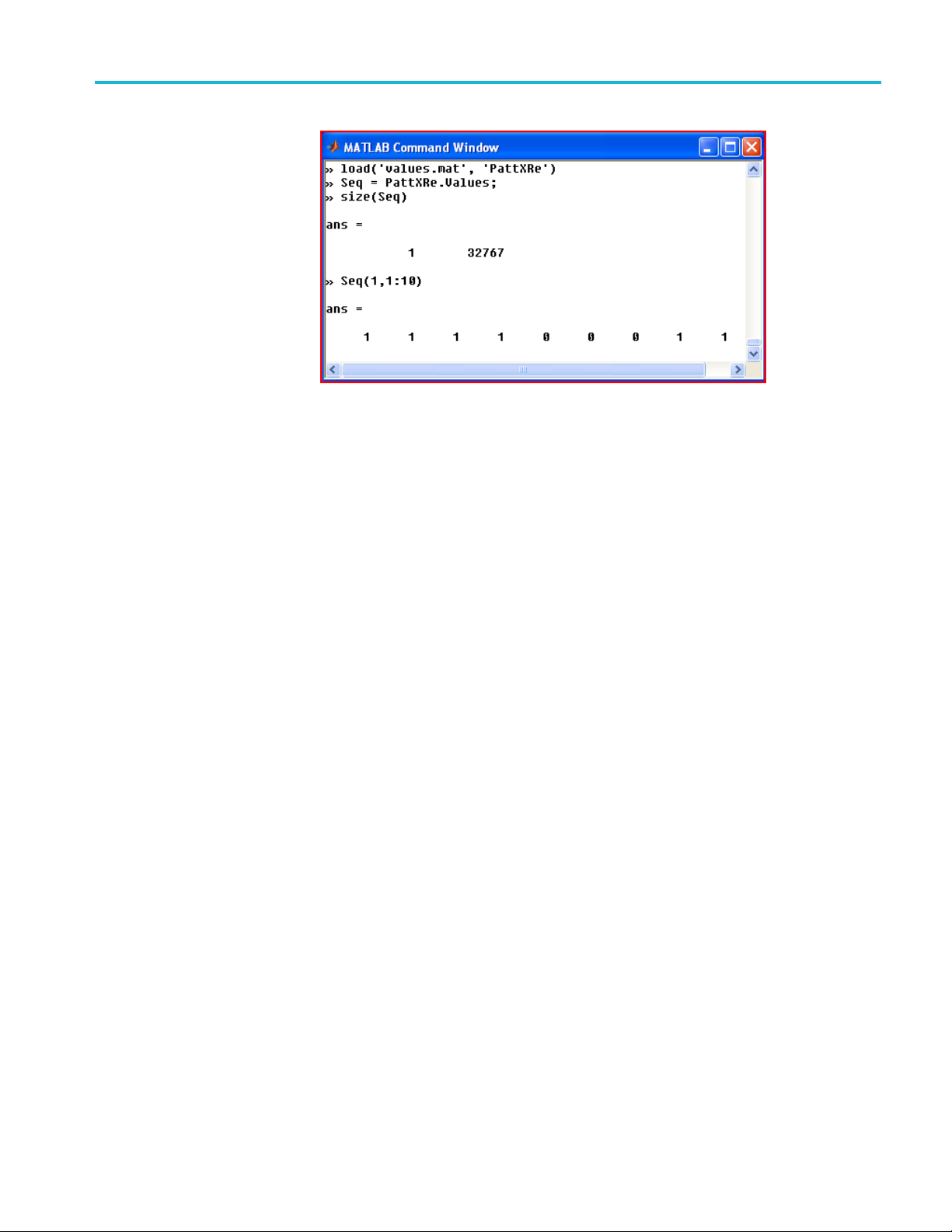
Analysis Parameters control and conﬁguration tab

In the case shown, a previously saved .mat ﬁle is loaded and the Seq variable is created using the PattXRe.Values content. The ﬁgure also shows the resulting size of the Seq variable and the ﬁrst 10 values. The pattern for each tributary may have any lengt

h, but must be a row vector containing logical values.

Synchronizing a long pattern can take a long time. The easiest way to keep calcula

tions fast when using non-PRBS patterns longer than 2

, and if using record lengths long enough to capture a t least as many bits as in the pattern, is to simply use the .SyncFrameEnd ﬁeld as shown above. Otherwise contact customer support for help in optimizing the synchronization.

Example capturing unknown pattern

Another way to load the pattern variable when using a pattern that is not one of the PRBS selections is to use the OMA to c apture the pattern and store it in a variable. Do the following:

1. Connect the optical signal with the desired modulation pattern to the OMA.

2. Set up the Analysis Parameters properly except for the data pattern which

is not yet known.

3. Choose Unknown as the data pattern (do not choose “User Pattern” yet).

Optimize the signal for open eye-diagrams and low EVM so that no errors are expected.

4. Set the record length long enough to capture the entire data pattern. For

example, you need 32,767 bits to capture a 2 28 Gbaud and the oscilloscope has a sampling rate of 50 Gs/s, then you need at least 32,767*50/28 = 58,513 points in the record. Stop acquisition after successfully displaying a good constellation with an adequate record length. All the data you need is now in the MATLAB workspace. It just needs to be put in the proper format for use in the pattern variable.

5. In the separate MATLAB Command Window, add the following commands:

15-1

pattern. Soifthisisat

OM1106 Analysis Software User Manual 63

Analysis Parameters control and conﬁguration tab

For QPSK:

PattXReM = real(zXSymUI.Values) > 0; PattXImM = ima

For dual-pol QPSK add these commands: (in addition to above)

PattYReM = real(zYSymUI.Values) > 0; PattYImM = imag(zYSymUI.Values) > 0;

6. To get a single full pattern, delete the extra data as follows (in this case for 32,767 bits):

For QPSK:

PattXReM = PattXReM(1: 32767); PattXImM = PattXImM(1: 32767);

For dual-pol QPSK add these commands: (in addition to above)

PattYReM = PattYReM(1: 32767); PattYImM = PattYImM(1: 32767);

g(zXSymUI.Values) > 0;

7. In the MATLAB Engine Command Window, add the following lines before the CoreProcessing statement:

For QPSK:

PattXRe.Values = PattXReM; PattXIm.Values = PattXImM;

For dual-pol QPSK add these commands: (in addition to above)

tYRe.Values = PattYReM;

Pat PattYIm.Values = PattYImM;

lect User Pattern for any of the tributaries where you assigned a user

8. Se pattern in the above steps. You should now be able to measure BER using your new patterns.

9. To save the patterns for later use, type the following in the separate MATLAB Command Window:

save(‘mypatterns.mat’,’PattXReM’, ’PattXImM’, ’PattYReM’, ’PattYImM’)

64 OM1106 Analysis Software User Manual

The Multicarrier Setup window

The Multicarr

ier Setup window

The Multicar an automatic scan, and to deﬁne which channels to include in the separate Multicarrier Eye and Multicarrier Conste llation axis plots. The window is divided into two sections: Multicarrier channel list and Multicarrier display layout. The absolute channel list is shown on the right, the relative version on the left.

WhentheMCSfeatureisenabledintheUSBHASPkey,theOMAdisplaysthe Multicarrier Setup button on the Setup ribbon.

Click the Multicarrier Setup button to open the Multi Setup window.

NOTE. Click the Multi Carrier setup button in the Layout region of the Home tab

to quickly arrange the screen for multicarrier measurements.

rier Setup tab deﬁnes the carrier channel plan, to start and stop

Figure 5: Multicarrier setup window

OM1106 Analysis Software User Manual 65

The Multicarrier Setup window

Multicarrier channel list

The main part of this section is the channel deﬁnition table. There are two types of channel deﬁnition table: absolute and relative. The default table type is absolute. A relative table may be entered by selecting Channel List Options: Add channel list: Add a new relative channel list. With an absolute channel deﬁnition table the channel of 195 THz. If the table is relative then the frequencies refer to the difference between the channel frequency and the current local oscillator frequency. Relative frequencies are speciﬁed in gigahertz.

The absolute channel deﬁnition table has four columns:

The Channel column contains an integer identifying the channel. The values in this column do not have to be consecutive. The Frequency column contains the absolute channel frequency.

The Preferred LO is the frequency that the local oscillator (also called the Reference Laser) is tuned to during an automatic scan to observe that channel. If the bandwidth of the multicarrier channels are so large that only one channel can be observed at a time given the bandwidth of the oscilloscope, then t channels have smaller bandwidth, then several table rows may be set to the same Preferred LO (even though the Frequency is different) so that all those channels are captured at the same local oscillator setting. This can save time, because tuning the local oscillator may be slow.

frequencies speciﬁed are the actual optical frequencies, in the region

he Preferred LO is typically set to the same value as Frequency. If the

The OMA identiﬁes the channel by the difference between its absolute frequency (in the Frequency column) and the LO frequency.

The ﬁnal column decides whether a channel is included in the automatic scan. Therelativechanneldeﬁnition table has only three columns. The second column, called Offset Frequency, contains the difference frequency between

he channel and current local oscillator frequency.

NOTE. The terms “Reference Laser” and “Local Oscillator” (LO) are used

interchangeably in the OMA and LRCP. The term LO is used here and in the channel list because it is more compact.

When the Add Channel button is pressed a new table row is added. The new entry has a Channel number one higher than the previous entry. The frequency columns contain values that increment from the previous row by an amount equal to the difference between the previous row and the row preceding that. The user is free to edit all the new row’s values. A table entry is removed by clicking on that row and pressing delete on the keyboard.

66 OM1106 Analysis Software User Manual

The Multicarrier Setup window

Multicarr

You c a n ent e r se the top left to select which one to apply. You can delete tables from the Channel List Options button.

The Scan Single button and Scan Run-Stop buttons start single and continuous automatic scans respectively. The OMA may take many acquisitions at each LO setting during the automatic scan, according to the Acquisitions per frequency control.

ier display layout

This section sets which plots to add in the separate axis plots, and how to arrange the subplots. The Automatic layout check box (enabled by default) lets OMA decide ho region below becomes active. You can choose the number of columns and rows of subplots either from the named controls, or by moving the horizontal and vertical sliders. Use the drop-down menu to select the channel number to be plotted in each subplot.

veral channel deﬁnition tables, and use the drop-down menu at

w to arrange the subplots. When Automatic layout is not checked, the

OM1106 Analysis Software User Manual 67

The Receiver Test conﬁguration tab

The Receiver T

est conﬁguration tab

Click the Rec for setting u p the OMA for receiver tests, and includes checks to verify that the receiver test is ready to run, and receiver-related test parameters settings. Click a parameter to display a brief explanation of that item in the lower help text pane.

NOTE. Use the Receiver Test button on the Home Ribbon to display the correct

plot and control tabs for Receiver Test operation.

NOTE. Receiver tests require a Tektronix OM2210.

eiver Test button to open the RXTest conﬁguration tab. This tab is

68 OM1106 Analysis Software User Manual

The Receiver Test conﬁguration tab

Table 7: RXTest

Parameter Description

Start wavelen

Stop wavelength The unit must be the same for Start, Stop, and Step. Enter the

Step The unit must be the same for Start, Stop, and Step. Enter the

Heterodyn

Skew measurement range Skew is measured ﬁrst to enable measurement of phase angles

Total harmonic distortion

X-Y and I-Q skew each Step

parameters

gth

e Frequency

Choose units a If using channel numbers, they are based on the grid chosen above.

value for the last wavelength in the scan.

value of the increment between steps in the scan.

Target heterodyne difference frequency between Signal and Reference lasers at each wavelength step.

with skew removed. The skew is calculated by measuring phase over the f

Check the box to include THD measurement. Additional laser tuning i included. See settings for heterodyne target in Additional Parameters.

Check the box to measure the skew values at each wavelength step. Measuring skew values adds substantial test time d ue to the

ional frequency s weeps.

addit

nd enter the starting value for the wavelength scan.

requency range indicated and extracting the slope.

s necessary for the heterodyne frequency target if

Laser grid spacing

Minimum expected system

width

band

Heterodyne frequency tolerance

Number of averages per step

requency sweep step size

THD measurement frequency

THD frequency tolerance The laser frequencies are adjusted to obtain the target heterodyne

The laser grid is set to the speciﬁed value to allow for continuous

g between grid frequencies. The grid is set back to the original

tunin value when the test is complete.

easurement stops if a low signal is detected within the

The m minimum expected system bandwidth of the combined coherent receiver and oscilloscope system.

The laser frequencies are adjusted to obtain the target heterodyne frequency to within this tolerance before taking data. Keeping

onsistent heterodyne frequency removes frequency domain

ac effects from the wavelength plots. Tolerance below 200 MHz will increase test time.

The number of measurements to average when computing each wavelength entry for the calibration table.

Frequency step size for the skew measurement frequency sweep.

The heterodyne frequency target for the THD test.

frequency to within this tolerance before taking data. Keeping a consistent heterodyne frequency results in greater reproducibility. Tolerance below 200 MHz will increase test time.

OM1106 Analysis Software User Manual 69

The Receiver Test conﬁguration tab

Table 7: RXTest parameters (cont.)

Parameter Description

Estimated laser line width

Oscilloscope record length The number of points to be acquired by the oscilloscope for each

TIA gain control mode

Use default folder location The M ATLAB results of the RxTest run are stored in the default

Sweep Range for Frequency Response

Include P and N measurements

This value is only used for the calculation of the entries for the calibration table output ﬁle, pHybCalib.mat. The laser linewidth is used to help in recovering the phase of the heterodyne signals.

measurement. 200,000 is recommended when producing a pHybCalib.mat ﬁle during a wavelength sweep. Shorter record length down to 20,000 is faster for other measurements

If the receiver has a Transimpedance Ampliﬁer, it must be set to constant gain mode to provide meaningful results for some measurements.

directory if this is checked. Otherwise, the user is prompted for a location and ﬁle information. A dialog box will indicate the destination folder at the end of the run.

The highest frequency to include in the frequency response measurement. Measurement will start at this modulation frequency and stop at 500 MHz.

If your receiver has differential outputs, you may chose to include the P, N, or both P and N outputs in the measurement. If including both, you are prompted to reconnect cables twice during the measurement unless the Tri Mode probe is selected.

P and N measurements are only a llowed for the test versus Modulation Frequency. The Wavelength Sweep test assumes P outputs only.

Find low frequency cutoff If checked, the oscilloscope settings are changed to measure very

low frequencies to calculate a low cut off frequency. Because of laser frequency drift, many data acquisitions are required to obtain low frequency data. As a result, this test can take a signiﬁcant amount of time (> 30 minutes).

Use Tri Mode probe

If this is checked and P/N measurements are included, a command is sent to the oscilloscope to switch the Tri Mode probe between inputs A and B to measure the P and N outputs of the differential receiver.

70 OM1106 Analysis Software User Manual

The Receiver Test conﬁguration tab

To perform a re

ceiver test

NOTE. Receiver tests require a Tektronix OM2210 Laser Calibration Source and

the appropriate power meter software loaded.

NOTE. Only real-time DPO/MSO70000 series oscilloscopes are supported for the

Receiver Test application at this time.

If the rece P and N measurements are supported for all frequency response measurements. Wavelength sweep measurements assume that only P outputs are connected.

iver DUT has differential P and N outputs, connect the P outputs ﬁrst.

Hardware readiness

checks

OM1106 Analysis Software User Manual 71

To initiate a wavelength sweep to measure parameters such as quadrature phase angle vs. wavelength, it is necessary to conﬁgure the OMA for the hardware set up and the measurement parameters such as start and stop wavelength. Click Home > Receiver Test to lay out the screen and open the RxTest tab that has all of the conﬁguration settings.

Complete the Readiness Checks in the upper part of the RxTest tab by identifying the required hardware:

The Receiver Test conﬁguration tab

1. Click the ‘Click to Select Reference Laser’ link in the Readiness Checks

2. Click the ‘Click to Select Signal Laser’ link in the Readiness Checks area. Use

area. Use the LRCP controls to select and connect to the laser to be used as the Ref the Reference (using the drop down menu in the LRCP tab). The Reference Laser readiness status changes to a green check mark when the connection to the instrument is conﬁrmed.

the LRCP controls to select and connect to the OM instrument to use as the Signal Laser/Polarization switch inputs. Select it as the Signal Laser (using the drop down menu in the LRCP tab). The Signal Laser readiness status changes to a gr

erence Laser (also called the Local Oscillator or LO). Select it as

een check mark when the connection to the instrument is conﬁrmed.

3. Click the Scope Connect button. If you are using a DPO720004C or

r model real-time scope, makes sure that the Scope Service Utility on

late the oscilloscope is installed and running before connecting OMA to the oscilloscope. For older oscilloscopes, use the TekVISA connection method. (See page 3, To install TekVISA software.)

4. When connecting to the oscilloscope using the Connect button, set which receiver outputs are connected to which oscilloscope inputs, and enable all of the channels to be measured. Wavelength sweeps require four channels, and the Modulation Frequency test allows two or four channels.

5. Once connected, OMA populates the Rx Output Channel Map/ Filter area. Verify that the receiver DUT is connected to the speciﬁed scope channels. Each receiver output may have a ﬁlter designated. The ﬁlter may be constructed using SDLA or other methods to correct for ﬁxture frequency response and skew.

6. Enter the serial number and multiplier value of the USB Power Meter in the Power Meter S/N and Multiplier ﬁelds to satisfy the ﬁnal readiness check. If the green check mark doe s not appear, it u sually means there is a connection or driver p roblem with the power meter. The multiplier is the power ratio between the DUT signal input ﬁber and the Power meter ﬁber. Normally, a 90/10 splitter is used with 90 percent of the power going to the DUT, so the default value is 9. However, for sensitive receivers, you may

72 OM1106 Analysis Software User Manual

The Receiver Test conﬁguration tab

swap the connec Multiplier would be 0.111.

7. Once all of the all of the Readiness Checks, OMA enables the Start Test button.

tions to get lower power at the DUT input. In this case the

hardware is conﬁgured and green check marks are showing for

OM1106 Analysis Software User Manual 73

The Receiver Test conﬁguration tab

Receiver test r

eadouts

Table 8: Receiver test readout tabs

Readout Description

Optical Test Results The Optical Test Results panel shows the progress and status of the test. The details

panel below t using the arrow button to the far right of the “Details” title.

RxTestNumOut The Rx Test Num Out panel shows the worst case values versus wavelength for each of

the measu are displayed in each row.

he progress bars can be opened to view intermediate results or hidden

rements listed. The value and the wavelength where that value was measured

74 OM1106 Analysis Software User Manual

The Receiver Test conﬁguration tab

Wavelength Sweep

measurements

1. Select Test Vs. the wavelength sweep.

2. Set “X-Y and Itest time, but provides complete frequency response data over the “Skew measurement range” in addition to wavelength data for each wavelength tested.

NOTE. For receivers with automatic gain control, it is important to set the gain

control to ﬁxed gain. If the automatic gain control loop is operating, it will confuse calculations such as receiver gain. Some tests such as Skew will still function with automatic gain control, but it is best to switch it off.

3. Click Start Test to begin the wavelength sweep.

The test time depends on the selected parameters and settings. If they are selected, the following steps are performed:

1. Set laser grid. The laser tuning grid must be set to a value low enough to permit continuous tuning between grid points. 10 GHz and 12.5 GHz grid spacings are available. The grid is set back to the original setting at the end of the test.

2. Find frequency error. The lasers may have a ﬁxed frequency error (an offset between the laser frequency setting and the actual laser frequency). This

asured by the oscilloscope after the lasers are tuned to a particular

is me frequency offset.

Wavelength (RXTest tab, Test Parameters area) to perform

Q Skew each step” to True. This substantially increases

3. Mea

4. Measure phase and amplitude data at frequency target. To remove the effect

5. Measure THD at the THD frequency target. The lasers are re-tuned to

NOTE. OIF-DPC-Rx 01.2 speciﬁes a frequency target of 1 GHz and tolerance of

0.1 GHz for this measurement

sure skew. To extract the receiver phase angles, it is necessary to ﬁrst deskew the system. If the oscilloscope and cables have already been deskewed, then the skew measured will be that of the DUT. This is only measured once at the starting wavelength unless the “X-Y and I-Q Skew each step” is selected. The skew values are determined by performing two laser heterodyne frequency sweeps, one for each polarization.

of frequency response on a wavelength sweep, t he lasers are tuned to the same heterodyne frequency at each wavelength step as determined by the Heterodyne Frequency target. The measurements are repeated ﬁve times by default unless changed in the Additional Parameters section. Values outside the speciﬁed tolerance a re omitted.

the heterodyne frequency speciﬁed by the THD frequency target. THD is measured. Values outside the speciﬁed THD frequency tolerance are omitted.

OM1106 Analysis Software User Manual 75

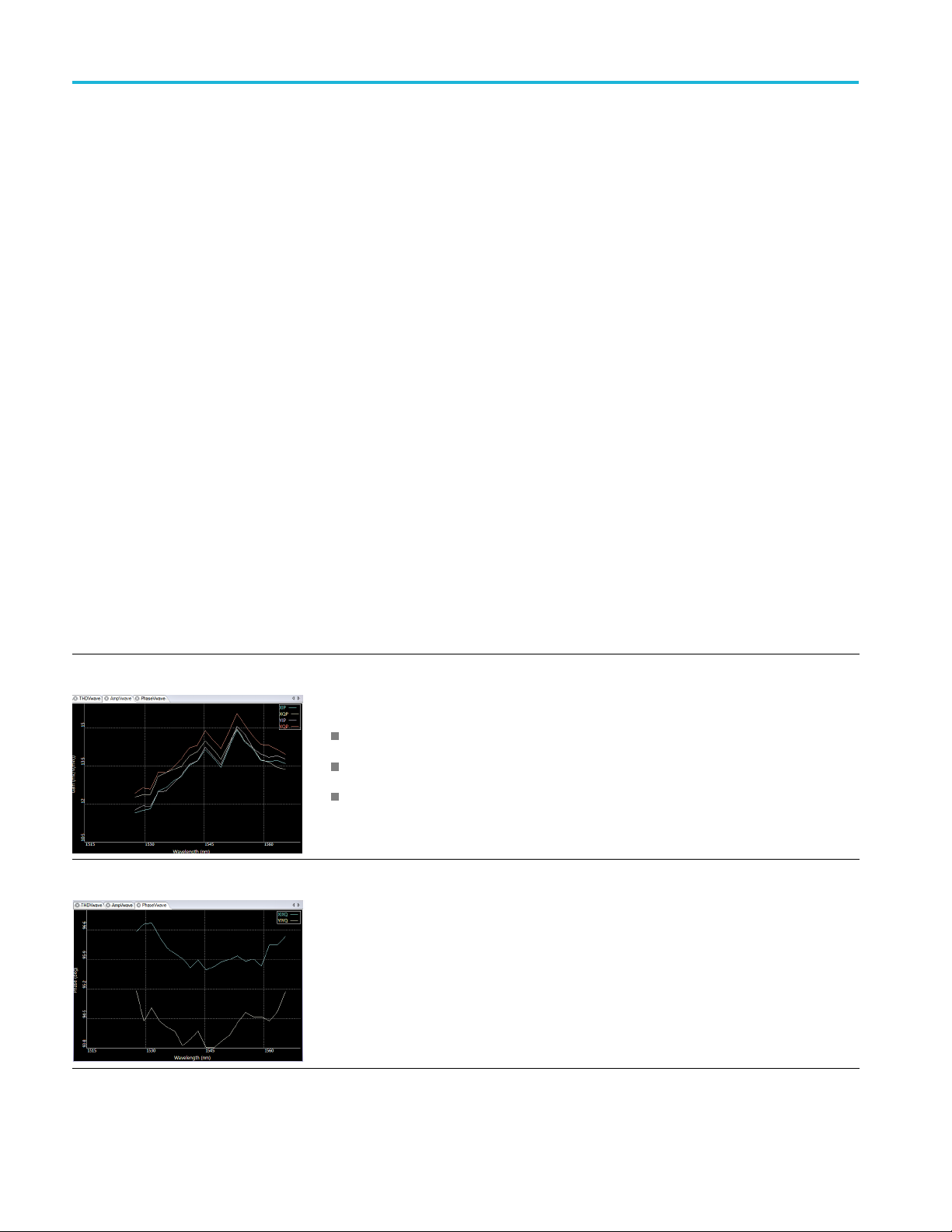
The Receiver Test conﬁguration tab

The test status

is shown in the Optical Test Results tab. At the end of the test, the data is shown in the plots. The RxTestNumOut tab displays the worst-case measurements that were the found during the wavelength sweep.

Optical hybrid calibration. TheWavelengthSweepmayalsobeusedtoproducea calibration ﬁle called pHybCalib.mat which is used by the OMA. This ﬁle is used to correct for coherent receiver impairments when the receiver is being used as part of an Optical Modulation Analysis (OMA) system. You may indicate where this ﬁle should be stored using the “Use default folder location” check box in the Additional parameters section. If this is not checked, you will be prompted for a storage location and info about the device to be stored in the ﬁle.

If you have previously used our Hybrid Receiver Calibration (HRC) software, you may wish to see the plots in this format for comparison against past results. These plots are still available for backward compatibility. To see the HRC plots, type ‘ShowHRCplots = true;’ in the separate Matlab application window (do not enter the quote marks).

Wavelength sweep plots. All wavelength s weep plots assume the DUT has single-ended outputs or that only the P-outputs are connected if the DUT has differential outputs.

You can measure wavelength properties of the N-outputs if these ports are connected to the oscilloscope. The results are plotted and reported as P-outputs.

Table 9: RxTest: Wavelength sweep plots

Plot Description

Amplitude Vs. Wavelength

Phase Vs. Wavelength

Gain for e ach channel is computed based on the measured input power and output voltages when the DUT is excited by two orthogonal signal input states.

Right-click options:

Gain in mV per √mW of signal power

Relative gain from channel to channel

Turn traces and markers on and off

The effect of skew is removed to provide the phase angle near zero modulation frequency. The signal input polarization state which provides the highest SNR is chosen for the phase measurement.

Right-click options: Turn traces and markers on and off.

76 OM1106 Analysis Software User Manual

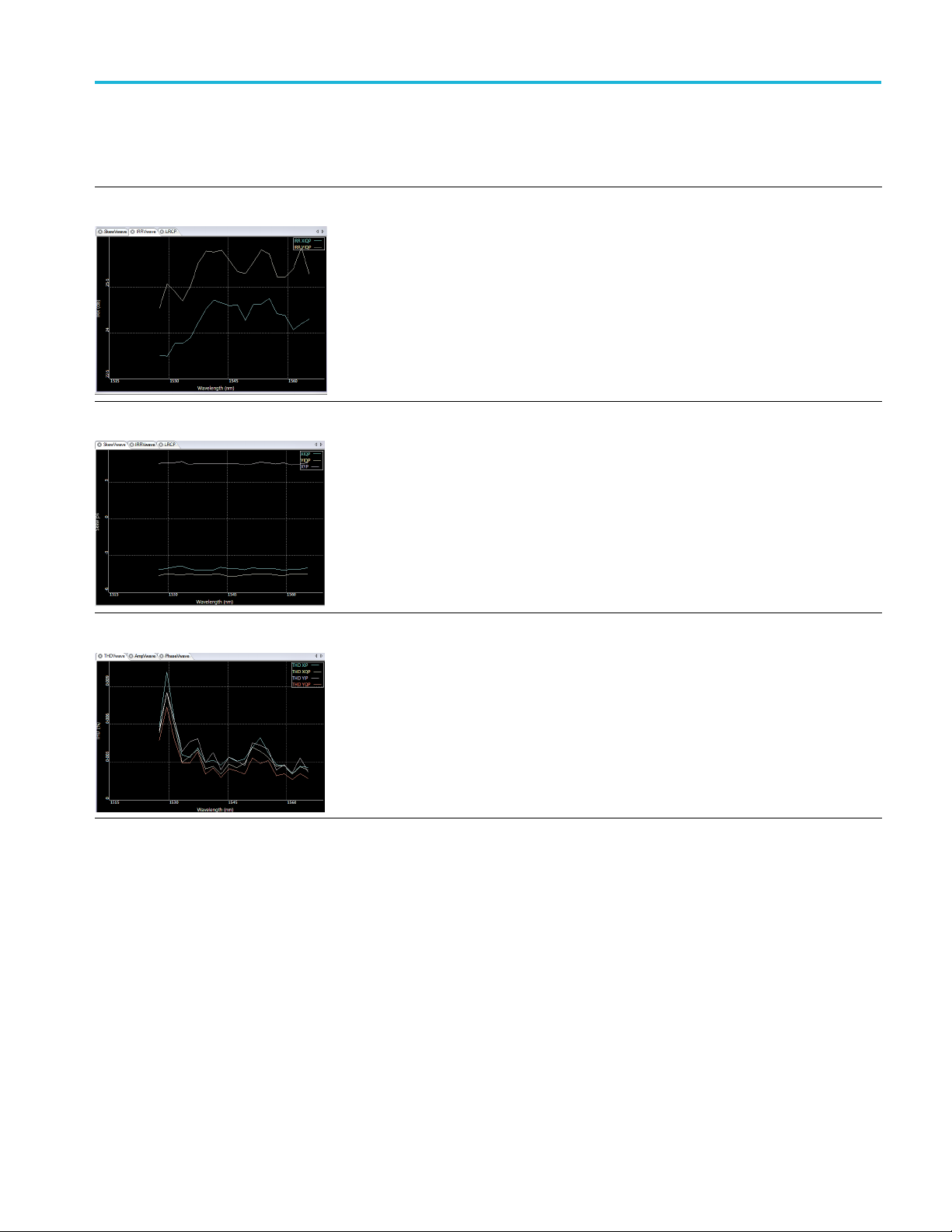
The Receiver Test conﬁguration tab

Table 9: RxTest: Wavelength sweep plots (cont.)

Plot Description

IRR Vs. Wavelength

Skew V s . Wavelength Check the RxTest control “X-Y and I-Q skew each step” to get valid Skew Vs. Wavelength

The image rejection ratio is found by taking 10 times the log10of the power ratio at the signal and image frequencies at the target heterodyne frequency. The effect of skew is not removed from this measurement. Deskew the oscilloscope and test ﬁxture using the oscilloscope UI or by providing the appropriate De-embed ﬁlter to get the best result for the DUT.

Right-click options: Turn traces and markers on and off.

data for each wavelength measured. Unchecking this box will yield valid data only at the ﬁrst wavelength. The effect of skew is not removed from this measurement. Deskew the oscilloscope and test ﬁxture using the oscilloscope UI or by providing the appropriate De-embed ﬁ lter to get the best result for the DUT.

Right-click options: Turn traces and markers on and off.

THD Vs. Wavelength

Modulation frequency

sweep measurements

The Total Harmonic Distortion (THD) is measured at the target heterodyne frequency with the tolerance speciﬁed in the RxTest Additional Parameters area.

NOTE. OIF-DPC-Rx 01.2 speciﬁes a frequency target of 1 GHz and tolerance of

0.1 GHz for this measurement

The modulation frequency sweep measurements perform a heterodyne frequency sweep to ﬁnd the frequency response of the receiver at a particular wavelength. The term “Modulation Frequency” is used in contrast to measurements vs. optical wavelength. The modulation used is the heterodyne beat frequency between the Signal and Reference laser frequencies.

Many of the modulation frequency tests can be performed during a wavelength sweep, so that both modulation and optical properties can be measured simultaneously. The separate Test Vs. Modulation Frequency provides a more in-depth analysis at a particular wavelength.

OM1106 Analysis Software User Manual 77

The Receiver Test conﬁguration tab

“Include P and N vs. Modulation Frequency enables testing of P and N response. Check “Use TriMode probe” if you will use a TriMode probe to connect to the P and N outputs of the DUT. The A input should be connected to the DUT “P” output. If a TriMode probe is not available for each channel, the P and N responses can still be measured by moving the cable connections as prompted by the OMA. The OMA prompts calculation of P vs N measurements such as P-N skew.

NOTE. For receivers with automatic gain control, it is important to set the gain

Select the modulation test to perform, set a ny parameters, and click Start Test to run the modulation frequency sweep measurements.

The test time depends on the options selected. If they are selected, the following steps are performed:

1. Set laser grid. The laser tuning grid must be set to a value low enough to

permit continuous tuning between grid points. 10 GHz and 12.5 GHz grid

ings are available. The grid is set back to the original setting at the end of

spac the test.

measurements:” Unlike the Test vs. Wavelength, the Test

the user to change the cable connections two times. This permits

2. Fin

3. Measure frequency response over indicated sweep range with indicated step

4. Toggle TriMode probe or prompt user to move cable connections if P and N

5. Measure low frequency cutoff. If this feature is selected, the lasers tune to

The test status is shown in the Optical Test Results tab. At the end of the test, the data is shown in the plots. The RxTestNumOut tab displays the worst-case measurements found during the testing.

d frequency error. The lasers may have a ﬁxed frequency error (an offset between the laser frequency setting and the actual laser frequency). This is measured by the oscilloscope after the lasers are tuned to a particular frequency offset.

size. A subset of the “Sweep range for frequency response” may be speciﬁed as the “Sweep range for skew measurement” if desired.

are to be measured. Repeat step 3 two times.

the same frequency and data is collected at a very low sample rate to ﬁnd the low frequency corner of the DUT. Because of laser frequency drift, many data acquisitions are required to obtain low frequency data. As a result, this test can require a signiﬁcant amount of time (> 30 minutes). Given the long test time, this test is omitted from the P/N testing loop. Repeat the test as needed to measure P and N low frequency cutoff.

78 OM1106 Analysis Software User Manual

The Receiver Test conﬁguration tab

Modulation fre

quency sweep plots. All of the frequency sweep plots have

right-click options to display P, N, or both P and N measurements (if available). Set P, N, or P+N data collection in the RxTest control.

Table 10: RxTest: Modulation Frequency sweep plots

Plot Description

Amplitude Vs. Frequency

Phase Vs. Frequency

Gain for each channel is computed based on the measured input power and output voltages when the DUT is excited by two orthogonal signal input states.

Right-click options:

Gain in mV per √mW of signal power

Relative gain from channel to channel

Amplitude and relative amplitude

Turn traces and markers on and off

The effec frequency, or included to see the effect and measurement of skew. The signal input polarization state which provides the highest SNR is chosen for the phase measurement.

Right-c

t of skew can be removed to provide the phase angle near zero modulation

lick options:

Phase (d

egrees)

IRR Vs. Frequency

Phase w

Phase E

Turn tr

The image rejection ratio is found by taking the power ratio at the signal and image frequencies at the target heterodyne frequency. The effect of skew is not removed from this measurement. Deskew the oscilloscope and test ﬁxture using the oscilloscope UI or by providing the appropriate De-embed ﬁlter to get the best result for the DUT.

Right-click options:

Turn traces and markers on and off

ith skew effect removed

rror with skew effect removed

aces and markers on and off

OM1106 Analysis Software User Manual 79

State controls

State control

The State con state parameters to an .xml ﬁle. When hardware state information is loaded, an IP connection will be made to the target hardware so that it can be conﬁgured. This means that the hardware must be at the same IP address as it was when the state was saved or the IP address must be updated using the Optical Connect > Auto Conﬁgure feature. Using reserved or ﬁxed IP addresses will make it easier to reliabl

The OMA software state information consists of the following:

All Analysis Parameters Settings

Record Length and Block Size

Auto Connect State and Auto Conﬁgure State from scope connect dialog box

Matlab window contents

OUI glo

Reference laser frequency

The OMA hardware state information consists of the following:

trols save or load the current OMA system hardware and/or software

y restore hardware conﬁguration.

bal display scales

All LRCP settings are considered hardware settings. The Reference laser frequency is considered a software setting as well so will be loaded if either a hardware or software state is loaded

Information needed to connect to the scope such as IP address

All oscilloscope settings are part of the hardware state. These are saved on the target oscilloscope using a setup ﬁ le with the same name as the hardware state xml ﬁle

OMA system deskew values from the Calibration tab

Oscilloscope channel mapping and which channels are enabled

80 OM1106 Analysis Software User Manual

The Home tab

The Home tab lets you select the plots to display in the Plots panel.

Constellation plots

Click the Constellation plot button (in the Home controls) to display the

list of available plots.

Table 11: Constellation plots

Plot type Description

X, Y Constellation Displays the constellation diagram for X or Y signal polarization with numerical readout

bottom tabs. Symbol-center values are shown in blue. Symbol errors are shown in red. Right-click for other color options.

Right-click to see plot display options.

Intermediate X , Y Constellation Displays offset (intermediate) polarization plots. Both polarization and quadrature offset

s are available.

format

The Y polarization is a half-symbol offset from the X polarization; the s tandard “Y const” displayisempty.

OM1106 Analysis Software User Manual 81

TheHometab

Table 11: Constellation plots (cont.)

Plot type Description

3D X Constellation, 3D Y Constellation Displays 3D Constellation for X or Y signal polarization. Displays the constellation

diagram with a time axis. You can scale and rotate to view on a 2 D or 3D monitor.

Multicarrier X Constellation,

arrier Y Constellation (Requires

Multic

Option MCS)

About constellation

diagrams

Displays the constellation diagram for each multicarrier channel. This feature requires

MCS.

Option

As each channel is analyzed, only that part of the plot is updated while the most recent data displayed will continue to be shown in t he other regions so that an aggregate view of

ticarrier group is displayed. Use the Clear Data button to discard prior data.

the mul

The layout is controlled by the Multicarrier Setup window. (See page 65.)

e the laser phase and frequency ﬂuctuations are removed, the resulting electric

Onc ﬁeld can be plotted in the complex plane. When only the values at the symbol centers are plotted, this is called a Constellation Diagram. When continuous traces are also shown in the complex plane, this is often called by the more generic term of IQ Diagram. Since the continuous traces can be turned on or off in the OMA, we refer to both as the Constellation Diagram.

The scatter of the symbol points indicates how close the modulation is to ideal. The symbol points spread out due to additive noise, transmitter eye closure, or ﬁber impairments. You can measure the scatter by symbol standard deviation, error vector magnitude, or mask violations.

82 OM1106 Analysis Software User Manual

TheHometab

Constellation

measurements

Measurements m OMA. Numerical measurements are available on the ﬂyout panel associated with each graphic window and also summarized in the Measurements Panel. The available constellation measurements are:

Elongation: The mean inter-symbol spacing of the quadrature signals

divided by the mean inter-symbol spacing of the in-phase signals. “Tall”

constellations have Elongation > 1. This is related to IQ Gain Imbalance,

which is 1/Elongation expressed in dB. IQ Gain Imbalance is reported in the

Measurement Statistics plot.

Real Bias: The real part of the mean value of all symbols divided by the

magnitude; expressed as a percent. A positive value means the constellation

is shifted right. Another m easure of constellation bias is IQ Offset which is

reported in the Measurement Statistics plot.

Imag Bias: The imaginary part of the mean value of all symbols divided

by the magnitude; expressed as a percent. A positive value means the

constellation is shifted up.

Magnitude: The mean value of the magnitude of all symbols with units given

on the plot.

Phase Angle: The phase angle between the two tributaries. The deviation

from 90 degrees is reported in the Measurement Statistics plot as Quadrature

Error.

ade on constellation diagrams are the most comprehensive in the

StdDev by Quadrant: The standard deviation of symbol point distance from

the mean symbol in units given on the plot. This is displayed for BPSK

and QPSK.

EVM (%): The rms average distance of each symbol point from the ideal

symbol point divided by the magnitude of the largest ideal symbol expressed

as a percent.

EVM Tab: The separate EVM tab provides the EVM% by constellation

group. The numbers are arranged to correspond to the symbol arrangement.

Mask Tab: The separate Mask tab shown in the right ﬁgure provides the

number of Mask violations by constellation group. The numbers are arranged

to correspond to the symbol arrangement.

The Q calculation can cause alerts if it can’t calculate a Q factor for the outer transitions. For example, in 32-QAM. 32-QAM is a subset of 64-QAM, where the outer constellation points are never used. It is not possible to calculate a Q factor for those outer slices, hence the alert. The subconstellation identiﬁcation feature notices the unused constellation po constellation parameters (zXSym.Mean, zXSym.ConstPtMean, and so on), but that happens in EngineCommandBlock, after the Q calculation has occurred. QDecTh does not know that the outer constellation points never occur, and so it generates the appropriate alert, but it does continue processing. (See page 127, QDecTh.)

ints, and removes them from the relevant

OM1106 Analysis Software User Manual 83

TheHometab

Color features in

constellation plots

Right-click an Grade, Display Traces in Color Grade, and Color Key Constellation Points.

The Color Grade option provides an inﬁnite persistence plot where the frequency of occurr reveal patterns not readily apparent in monochrome. Use the right-click context menu in each plot to clear or set the color grade mode (requires nVidia graphic card on the PC).

y constellation plot to show a list of display options including Color

ence of a point on the plot is indicated by its color. This mode helps

Color Key Constellation Points is a special feature that works when not in Color Grade mode. The value of the previous symbol determines the symbol color. This helps reveal pattern dependence.

The Color Key colors:

If the prior symbol was in Quadrant 1 (upper right) then the current symbol is colored Yellow

If the prior symbol was in Quadrant 2 (upper left) then the current symbol is colored Magenta

If the prior symbol was in Quadrant 3 (lower left) then the current symbol is colored light blue (Cyan)

If the prior symbol was in Quadrant 4 (lower right) then the current symbol is colored solid Blue

84 OM1106 Analysis Software User Manual

TheHometab

Multicarrier constellation

plots (Requires Option

MCS)

The Multicarri icon button on the Home tab. These plots behave in a similar fashion to the existing constellation plots except that there are regions reserved for each channel. The layout is controlled by the Multicarrier Setup window described above.

This feature requires Option M CS.

As each channel is analyzed, only that part of the plot is updated while the most recent data displayed will continue to be shown in the other regions so that you can display an aggregate view of the multicarrier group. Use the Clear Data button to discard prior data.

er Constellation plots are accessed by clicking on the constellation

e 6: Multicarrier constellation plots

Figur

OM1106 Analysis Software User Manual 85

TheHometab

Eye plots

Click the Eye plot button (in the Home controls) to display the list of

available pl

Table12:Eyeplots

Plot type Description

X Eye, Y Eye

The coherent eye diagram for X or Y signal polarization shows the In-Phase or Quadrature components versus time modulo two bit periods. Click the Measurements bar at the bottom of the menu to display associated measurements.

Available X and Y Eye plots are:

ots.

Inphase Eye

Quadrature Eye

Differential Inphase Eye

Differential Quadrature Eye

Power Eye

Right-click the plot to list options including transition and eye averaging. The transition average shown in red is an average of each logical transition. The calculation is enabled in the Analysis Parameters tab and is used for calculating transition measurements.

Displays the computed power per polarization vs time modulo 2 bit periods. This is a calculation of the eye diagram typically obtained with a photodiode-input oscilloscope.

Available Power Eye plots are:

Power Eye

X Power Eye

Y Power Eye

Right-click the plot to list options including color grade.

86 OM1106 Analysis Software User Manual

TheHometab

Table 12: Eye plots (cont.)

Plot type Description

3D X Eye, 3D Y Eye Displays the 3D representation constellation diagram with a time axis modulo 2 bit

periods, for X or Y signal polarization. You can scale and rotate the plot to view on a 2D or 3D monitor.

Multicarrier X, Multicarrier Y Eye

teyediagrams

Abou

Displays eye plots for each channel. This feature requires Option MCS.

As each data displayed continues to be shown in the other regions to display an aggregate view of the multicarrier group. Use the Clear Data button to discard prior data.

The lay

channel is analyzed, only that part of the plot is updated while the most recent

out is controlled by the Multicarrier Setup w indow. (See page 65.)

Supported eye formats include ﬁeld Eye (which is simply the real part of the phase trace in the complex plane), Power Eye (which simulates the Eye displayed with a conventional oscilloscope optical input), and Diff-Eye (which simulates the

e generated by using a 1-bit delay-line interferometer). Right-click to select

Ey display color options.

e ﬁeld Eye diagram provides the following measurements:

Q (dB): Computed from 20*Log10 of the linear decision threshold Q-factor

ftheeye

Eye Height: The distance from the mean one level to the mean zero l evel

(units of plot)

OM1106 Analysis Software User Manual 87

TheHometab

Eye waveform averaging

Rail0 Std Dev: T

he standard deviation of the 0-Level as determined from the

decision threshold Q-factor measurement

Rail1 Std Dev:

The standard deviation of the 1-Level as determined from the

decision threshold Q-factor measurement

In the case o

f multi-level signals, the above measurements are listed in the order of the corresponding eye openings in the plot. The top row values correspond to the top-most eye opening.

The above functions involving Q factor use the decision threshold method described in the paper by Bergano

. When the number of bit errors in the measurement interval is small, as is often the cas e, the Q-factor derived from the bit error rate may not be an accurate measure of the signal quality. However, the decision threshold Q-factor is accurate because it is based on all the signal values, not just

thosethatcrossadeﬁned boundary.

N.S. Bergano, F.W. Kerfoot, C.R. Davidson, “Margin measurements in optical ampliﬁer systems,” IEEE P hot.

tt., 5, no. 3, pp. 304-306 (1993).

Tech. L e

Two types of averaged signal display are available for eye diagrams and signal vs. time. These show a cleaner version of the signal, having a reduced level of

ive noise. The transition average is available by checking Averaging: Show

addit Transition Average under Analysis P arameters and selecting Show Transition Average from the right click menu of the eye diagram where the average is to b e displayed. The red trace shows the average of the different transitions between levels: 0-0, 1-1, 0-1 and 1-0.

The transition parameters listed in the X-Trans, Y-Trans a nd Pow-Trans sections of the Measurements table are derived from the tra nsition average curves. Transition average is available for the ﬁeld component eye diagrams, and if the modulation format is an OOK type, for the power eye diagram.

88 OM1106 Analysis Software User Manual

Tektronix OM1106 Primary User

Specifications and Main Features

Frequently Asked Questions

User Manual