

Page 1

Keithley quickDAQ Quick Start Guide
1. Measurement setup ............................................................................................................1
2. Setting up to record multiple bands .....................................................................................3
3. Analyzing data....................................................................................................................4
4. Saving files .........................................................................................................................7
5. Playback of recorded files ...................................................................................................8
1. Measurement setup
Use the drop-down menu to select one of the supported thermocouple types:
J,K,B,E,N,R,S,T
Channel 0 (zero) is NOT
AVAILABLE for TC
measurements (it is only used
for cold junction
compensation, CJC,
measurements).
Updated 17-Nov-06 p. 1
Page 2

Use the Device tab to setup the basic configuration for data acquisition using the KUSB-3100
Module:
Only recorded data can be plotted. Use the Recording tab to setup the recording parameters:
Updated 17-Nov-06 p. 2
Page 3

2. Setting up to record multiple bands
Several “bands” are provided that can be used to simulate strip charts. These bands can be
configured to display multiple channels of data. Several parameters for these bands can be
programmed including a background color and trace color. Different data acquisition channels
can be assigned to these Bands, as shown below:
Updated 17-Nov-06 p. 3
Page 4
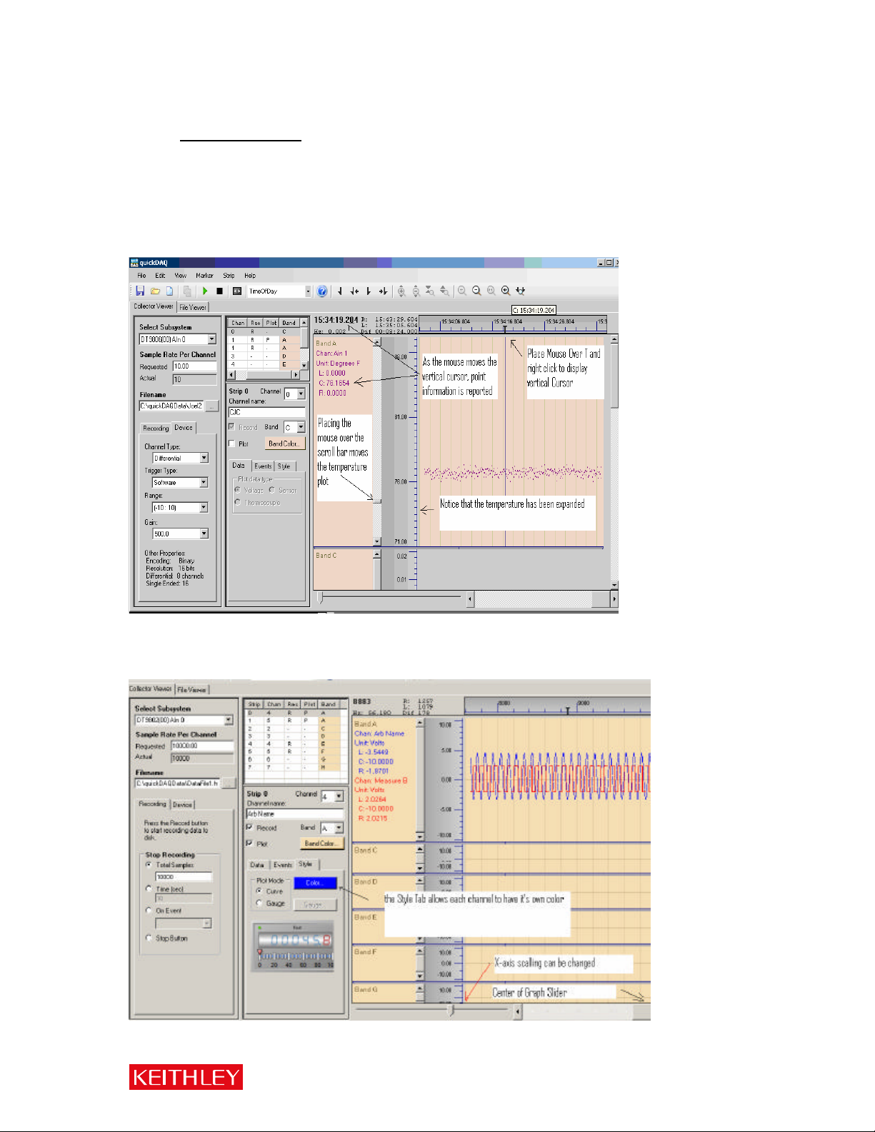
3. Analyzing data
Once data collection begins, the Y axis on the spreadsheet will be set to span the entire
temperature range for the selected Thermocouple. Change the Y-axis limits by placing the mouse
in the plotting area of the graph and pressing the mouse’s left button while the Ctrl Key is pressed
until an expanded arrow is presented. Once this expanded arrow is presented, moving the mouse
up or down compresses or expands the Y (Temperature) axis. This expanded axis can be
repositioned by moving the vertical slider bar at the left of the plot up and down as shown below.
The quickDAQ software provides scrolling and zoom capability allowing individual points from a
collected sample set to be read out easily. Shown below, is the result of configuring quickDAQ to
gather 10,000 points from each of two channels:
Updated 17-Nov-06 p. 4
Page 5
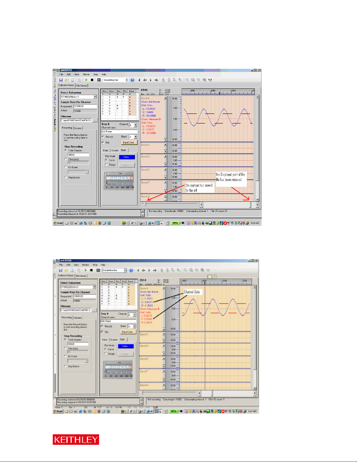
After the data has been collected, the Zoom axis (indicated by the slider at the lower left of the
graph) is positioned near its center. If the position of this slider is moved to the left, the X-axis can
be expanded to show more detail of each wave form:
The software provides vertical cursors that “read out” the value of each recorded point. One of
these vertical cursors can be selected by right clicking the mouse as it sits of the “T”. As this
cursor is slid left and right, the recorded data value is displayed along the left edge of the graph of
plot:
Updated 17-Nov-06 p. 5
Page 6
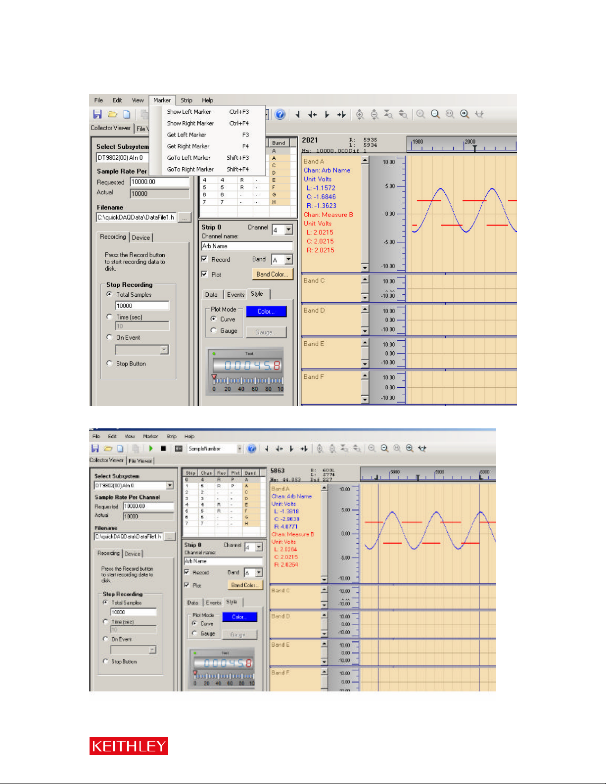
A Right and Left Vertical Scroll Bar are also available that provide a convenient way of saving
only the “interesting” section of a recorded file:
Once Right and Left Scroll Bars have been displayed they can be set at a desired location:
Updated 17-Nov-06 p. 6
Page 7
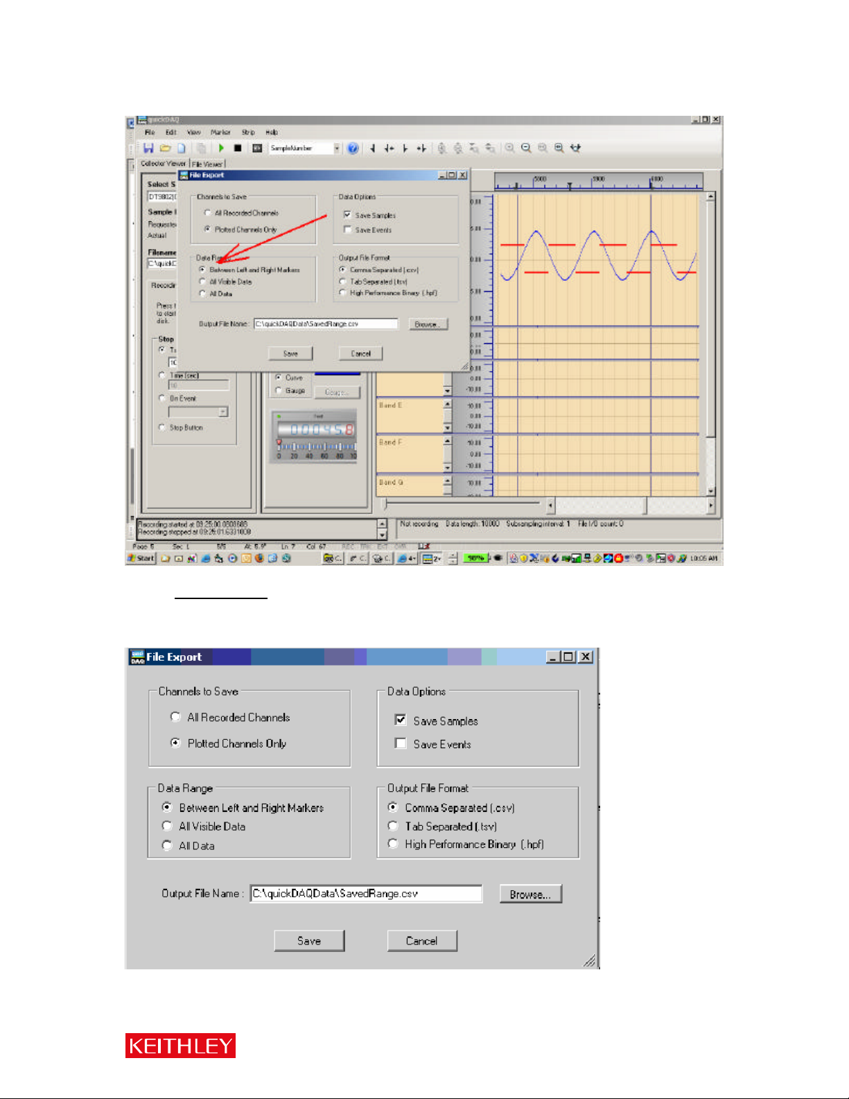
One use of these cursors is to define a subset of the data that can then be saved to file:
4. Saving files
Once the data has been collected, it can be stored in a variety of formats ( Comma Separated,
Tab Separated, or High Performance Binary.
Updated 17-Nov-06 p. 7
Page 8

5. Playback of recorded files
Using the OPEN menu, a previously created .HPF can be loaded into the quickDAQ software and
displayed:
Data can then be analyzed as described in Section 3 of this document.
Updated 17-Nov-06 p. 8
 Loading...