Tektronix IConnect,MeasureXtractor User Manual

Download

User Manual

IConnectR and MeasureXtractort TDR and VNA Software

071-1835-01

This document applies to software version 4.0 and above.

www.tektronix.com

Copyright © Tektronix. All rights reserved. Licensed software products are owned by Tektronix or its subsidiaries or suppliers, and are protected by national copyright laws and international treaty provisions.

Tektronix products are covered by U.S. and foreign patents, issued and pending. Information in this publication supercedes that in all previously published material. Specifications and price change privile ges reserved.

TEKTRONIX and TEK are registered trademarks of Tektronix, Inc.

IConnect is a registered trademark of Tektronix, Inc.

MeasureXtractor is a trademark of Tektronix, Inc.

Contacting Tektronix

Tektronix, Inc. 14200 SW Karl Braun Drive P.O. Box 500 Beaverton, OR 97077 USA

For product information, sales, service, and technical support:

H In North America, call 1-800-833-9200.

H Worldwide, visit www.tektronix.com to find contacts in your area.

Warranty 9(b)

Tektronix warrants that the media on which this software product is furnished and the encoding of the programs on the media will be free from defects in materials and workmanship for a period of three (3) months from the date of shipment. If any such medium or encoding proves defective during the warranty period, Tektronix will provide a replacement in exchange for the defective medium. Except as to the media on which this software product is furnished, this software product is provided “as is” without warranty of any kind, either express or implied. Tektronix does not warrant that the functions contained in thi s software product will meet Customer’s requirements or that the operation of the programs will be uninterrupted or error-free.

In order to obtain service under this warranty, Customer must notify Tektronix of the defect before the expiration of the warranty period. If Tektronix is unable to provide a replacement that is free from defects in materials and workmanship within a reasonable time thereafter, Customer may terminate the license for this software product and return this software product and any associated materials for credit or refund.

THIS WARRANTY IS GIVEN BY TEKTRONIX WITH RESPECT TO THE PRODUCT IN LIEU OF ANY OTHER WARRANTIES, EXPRESS OR IMPLIED. TEKTRONIX AND ITS VENDORS DISCLAIM ANY IMPLIED WARRANTIES OF MERCHANTABILITY OR FITNESS FOR A PARTICULAR PURPOSE. TEKTRONIX’ RESPONSIBILITY TO REPLACE DEFECTIVE MEDIA OR REFUND CUSTOMER’S PAYMENT IS THE SOLE AND EXCLUSIVE REMEDY PROVIDED TO THE CUSTOMER FOR BREACH OF THIS WARRANTY. TEKTRONIX AND ITS VENDORS WILL NOT BE LIABLE FOR ANY INDIRECT, SPECIAL, INCIDENTAL, OR CONSEQUENTIAL DAMAGES IRRESPECTIVE OF WHETHER TEKTRONIX OR THE VENDOR HAS ADVANCE NOTICE OF THE POSSIBILITY OF SUCH DAMAGES.

Getting Started

Operating Basics

IConnect Overview 1--1...............................................

What You Can Do With IConnect 1--3...................................

IConnect Installation Notes 1--5........................................

Adobe Acrobat Reader 1--6............................................

Manual Sentinel Hardware Key Driver Installation, Removal,

and Configuration 1--6............................................

Getting Started With IConnect 1--7......................................

IConnect Shortcuts 1--8...............................................

Enhancements and Improvements i n IConnect 4.0 1--10......................

Enhancements and Improvements i n IConnect 3.6 1--11......................

Preparing to Take Measurements 2--2....................................

True Impedance Profile (Z-Line) Computation Tutorial 2--6..................

What is True Impedance Profile? 2--6................................

True Impedance Profile in Failure Analysis 2--7........................

Measurements for Impedance Profile Analysis 2--7.....................

DUT Connections 2--9............................................

Setting up the Impedance Profile 2--10................................

Computing the Impedance Profile 2--10...............................

Using Cursor Readout 2--11.........................................

Using the Zoom Tool 2--12..........................................

Using Impedance Averaging 2--13....................................

Using Differential Impedance Profile 2--14.............................

Eye Diagram Tutorial 2--15.............................................

Waveform Acquisition and Setup 2--16................................

Choosing the Proper Termination 2--17................................

Selecting a Reference 2--18.........................................

DUT Connections 2--18............................................

Loading Data 2--19................................................

Display the Eye 2--21..............................................

Eye Diagram Options 2--22.........................................

Display the Final Eye 2--22.........................................

Eye Diagram Zooming 2--23........................................

Eye Masking Testing 2--24..........................................

Measure Jitter 2--24...............................................

Correlation 2--25..................................................

System Eye Diagram 2--27..........................................

S-Parameter Computation Tutorial 2--27..................................

IConnectR and MeasureXtractort 4. 0 User Manual

Table of Contents

What are S-Parameters? 2--27.......................................

Waveform Acquisition and Setup 2--28................................

S--Parameter Data Acquisition 2--29..................................

DUT Connections 2--30............................................

Differential, Common, and Mixed Modes 2--30.........................

Compute S--Parameters 2--32........................................

S--Parameter Options 2--33..........................................

Calibration 2 --34..................................................

Choosing the Data Display 2--34.....................................

Differential Example 2--35..........................................

Exporting Touchstone 2--37.........................................

Correlation 2--38..................................................

Lumped LC Computation Tutorial 2--39...................................

Waveform Acquisition and Setup 2--39................................

Measurement Setup Tips 2--40.......................................

Self Inductance 2--41..............................................

Self Capacitance 2--42.............................................

Mutual Inductance 2--43............................................

Mutual Capacitance 2--44...........................................

I/O Buffer Input Capacitance 2--46...................................

Simulate 2--46....................................................

Single and Coupled Line Modeling Tutorial 2--48...........................

Waveform Acquisition and Setup 2--48................................

DUT Connections 2--49............................................

Loading Data 2--50................................................

Computing Z--Line 2--51...........................................

Windowing the Data 2--52..........................................

Partitioning Details 2--53...........................................

Other Practical Details 2--54........................................

Symmetric Coupled Model Details 2--54...............................

Saving the Model 2--56.............................................

Simulating 2--57..................................................

PWL Source 2--58.................................................

Analyzing the Results 2--59.........................................

Risetime Filtering 2--60............................................

Lossy Line Modeling Tutorial 2--60......................................

Waveform Acquisition and Setup 2--61................................

Choosing the Extract Termination Type 2--62...........................

DUT Connections 2--62............................................

Loading Data 2--63................................................

Model Extraction 2--64.............................................

Model Accuracy 2--65.............................................

Other Practical Details 2--66........................................

Choosing the Output Format 2--67....................................

Saving the Model 2--67.............................................

Simulating 2--69..................................................

PWL Source 2--70.................................................

Analyzing the Results 2--71.........................................

Eye Diagram 2--72................................................

MeasureXtractor Modeling Tutorial 2--73.................................

IConnectR and MeasureXtractort 4. 0 User Manual

Waveform Acquisition and Setup 2--73................................

Choosing the Extraction Termination Type 2--74........................

DUT Connections 2--75............................................

Loading Data 2--76................................................

Model Extraction 2--78.............................................

Model Accuracy 2--78.............................................

Saving the Model 2--79.............................................

Simulating 2--81..................................................

PWL TDR Source 2--82............................................

Analyzing the Results 2--83.........................................

IConnect Measure- Model- Simulate Methodology

The Value of Measure-Model-Simulate 3--1...............................

Measure-Model-Simulate within IConnect 3--2............................

Measurement

Measurement Overview 4--1...........................................

GPIB Installation 4--1................................................

Running IConnect on the Tektronix DSA8200 and TDS/CSA8000 Series 4--2....

Oscilloscope Setup 4--3...............................................

Configuring IConnect to Communicate with your Instrument 4--3.............

Waveform Acquisition 4--6............................................

Saving and Restoring the Instrument Setup 4--10............................

Measurement Tips 4--11...............................................

Table of Contents

Models

Model Extraction Overview 5--1........................................

Model Extraction Tips 5--2............................................

Simple Source 5--3...................................................

PWL Source 5--3....................................................

PWL Source Measure Tab 5--4......................................

PWL Source Model Tab 5--4.......................................

Lumped 5--5........................................................

Passive Equalizer 5--6................................................

Lumped Coupled 5--7................................................

Single Line 5--9.....................................................

SingleLineMeasureTab 5--10.......................................

Single Line Model Tab 5--11........................................

Single Line Simulate Tab 5--13......................................

Symmetric Coupled Lines 5--14.........................................

Symmetric Coupled Lines Measure Tab 5--16...........................

Symmetric Coupled Lines Model Tab 5--18............................

Symmetric Coupled Lines Simulate Tab 5--20..........................

Lossy Line 5--21.....................................................

Lossy Line Measure Tab 5--23.......................................

Lossy Line Model Tab 5--24.........................................

Lossy Line Simulate Tab 5--27.......................................

Symmetric Coupled Lossy Lines 5--29....................................

IConnectR and MeasureXtractort 4. 0 User Manual

iii

Table of Contents

Symmetric Coupled Lossy Lines Measures Tab 5--30.....................

Symmetric Coupled Lossy Lines Model Tab 5--31.......................

Symmetric Lossy Lines Simulate Tab 5-- 35............................

Data Driven Models 5--36..............................................

Data Driven Measure Tabs 5--38.....................................

Data Driven Model Tabs 5--42.......................................

Data Driven Simulate Tabs 5--43.....................................

Data Driven Single Line 5--43...........................................

Data Driven Coupled Lines 5--45........................................

Generic 2-port 5--47...................................................

Termination 5--48.....................................................

Composite Model 5--49................................................

Composite Model Measure Tab and TDR/T Viewer 5--50.................

Composite Model Schematic Viewer 5-- 50.............................

Composite Model Simulate Tab 5--53.................................

Composite Model Eye Diagram Viewer 5--57...........................

Eye Diagram Computation and Mask Testing 5--58..........................

Waveforms for Eye Diagram Computation 5--59........................

Eye Diagram Options 5--60.........................................

Adding Crosstalk to an Eye Diagram 5--64.............................

Eye Measurements and Analysis 5--66.................................

Partitioning Waveforms in IConnect 5--71.................................

Simulation

Managing and Viewing Waveforms

The EZ Zline Viewer

Verification Overview 6--1............................................

Configuring IConnect to Communicate with your Simulator 6--2..............

IConnect Linear Simulator 6--4.........................................

Model Verification with Multiple Simulators 6--5..........................

Model Verification Tips 6--6...........................................

The Waveform Viewers 7--1...........................................

Waveform Selection 7--6..............................................

Waveform File Operations 7--8.........................................

Waveform Viewing Operations 7--10.....................................

Using Labels in the Waveform Viewers 7--12...............................

Importing and Exporting Waveform Data 7--15.............................

Importing and Exporting Tabular Data 7--15............................

Importing and Exporting S--Parameter Data in Touchstone Format 7--19.....

Opening the EZ Z-Line Viewer 8--1.....................................

The EZ Z-Line Viewer Window Elements 8--2............................

Golden Setup 8--4...................................................

Taking DUT Z-Line Measurements with a Golden Setup 8--8.................

Taking DUT Z-Line Measurements Without a Golden Setup 8--10..............

Adjusting for Instrument Drift 8-- 11......................................

Adjust to Position Feature 8 --12.........................................

IConnectR and MeasureXtractort 4. 0 User Manual

Waveform Computations

Waveform Computations Overview 9--1..................................

Waveform Filtering 9--3..............................................

Impedance Profile Computation 9--4.....................................

Step Spectrum Computation 9--7........................................

S-Parameter Computation 9--9.........................................

Capacitance and Inductance Computation 9--11.............................

Flip Waveform 9--16..................................................

Waveform Math 9--17.................................................

Utilities

Screen Capture 10--1..................................................

E-mail Utilities 10-- 2..................................................

User Options

Table of Contents

Self Inductance Computation 9--13...................................

Self Capacitance Computation 9--14..................................

Mutual Inductance Computation 9--15.................................

Mutual Capacitance Computation 9--16................................

General Options 11--1.................................................

Computation Options 11--2.............................................

Simulation Options 11--3...............................................

Waveform Viewer Options 11--5.........................................

Command Line Interface

Conventions 12--1....................................................

Formats 12--2........................................................

Limitations 12--3.....................................................

Syntax 12--3.........................................................

Example CLI Statements 12--10..........................................

Error Reporting 12--14..................................................

Troubleshooting Tips 12--17.............................................

Appendices

Appendix A: Troubleshooting A--1...............................

Overview A--1.......................................................

Installation problems A--1.............................................

Problems Viewing On-line Documentation A--1............................

GPIB Card not recognized A--2.........................................

Oscilloscope connection will not work A--2...............................

Simulation A--3......................................................

Printing A--4........................................................

Appendix B: References B--1....................................

Index

IConnectR and MeasureXtractort 4. 0 User Manual

Table of Contents

List of Figures

Figure 1--1: IConnect data analysis and model

validation windows. 1--1.....................................

Figure 2--1: Displaying the Acquisition window 2-- 2.................

Figure 2--2: Instrument Settings tab in the Acquisition

dialog box 2--3.............................................

Figure 2--3: Use Instrument Settings to match the

oscilloscope settings 2--4.....................................

Figure 2--4: Incorrect Acquisition Window. 2--5....................

Figure 2--5: Correct Acquisition Window 2--5......................

Figure 2--6: True impedance profile example 2--6...................

Figure 2--7: Using the true impedance profile 2--7...................

Figure 2--8: The Acquisition dialog box 2-- 8........................

Figure 2--9: DUT setup for differential reference, reflection,

and transmission 2--9.......................................

Figure 2--10: Selecting waveforms for the impedance profile

computation 2--10...........................................

Figure 2--11: The impedance profile as displayed in the

waveform viewer 2--11.......................................

Figure 2--12: The cursor readout for the computed impedance

profile waveform 2--12.......................................

Figure 2--13: Zooming in and out on a waveform view 2--13...........

Figure 2--14: The Single Line model button 2--13....................

Figure 2--15: Using the Single Line model viewer to measure

average impedance 2--14.....................................

Figure 2--16: Eye Diagram 2--15..................................

Figure 2--17: You can initiate a lossy line model from either the

Model menu or from the Model toolbar 2-- 17....................

Figure 2--18: Select Termination Type 2--18.........................

Figure 2--19: Measurement connection scheme 2--19..................

Figure 2--20: Loading waveforms into the Lossy Line model 2--20......

Figure 2--21: Instrument interface window 2--20.....................

Figure 2--22: The Display button in the Eye Diagram area 2--21........

Figure 2--23: Eye diagram display 2--21............................

Figure 2--24: Eye Diagram and Mask Options dialog 2--22............

Figure 2--25: Display the eye diagram 2--23.........................

Figure 2--26: Choose the zoom method 2--23........................

IConnectR and MeasureXtractort 4. 0 User Manual

Table of Contents

Figure 2--27: Select a polygon 2 --24................................

Figure 2--28: Display the eye measurements 2--25....................

Figure 2--29: Directly measured eye diagram response 2--25...........

Figure 2--30: Eye diagram response from TDT measurements 2--26.....

Figure 2--31: System used to measure and predict the

eye diagram 2--27...........................................

Figure 2--32: Mapping between scattering parameters and

TDR/T measurements 2--29...................................

Figure 2--33: Measurement termination scheme 2--30.................

Figure 2--34: Differential-Differential block of mixed mode

S-Parameters 2--31..........................................

Figure 2--35: Common-Common block of mixed mode

S-Parameters 2--31..........................................

Figure 2--36: Mode Conversion block of mixed mode

S-Parameters 2--32..........................................

Figure 2--37: Computing S-Parameter 2--33.........................

Figure 2--38: S-Parameter fields in the Computation dialog box 2--34...

Figure 2--39: Single-ended S21 data computed from

TDT measurement 2--35......................................

Figure 2--40: Differential S-Parameter example 2--36.................

Figure 2--41: The S(f) tab 2--36...................................

Figure 2--42: Exporting Touchstone data 2--37......................

Figure 2--43: Export a 2-port Touchstone file 2--37...................

Figure 2--44: Export a 4-port Touchstone file 2--38...................

Figure 2--45: Correlation example 2--38............................

Figure 2--46: Computation of L and C 2--39........................

Figure 2--47: Choosing self inductance computation from the

main menu 2--40............................................

Figure 2--48: Displaying a self inductance measurement 2-- 42..........

Figure 2--49: Displaying a self capacitance measurement 2--43.........

Figure 2--50: Displaying a mutual inductance measurement 2-- 44......

Figure 2--51: Displaying a mutual capacitance measurement 2--45......

Figure 2--52: Extracting I/O buffer capacitance 2--46.................

Figure 2--53: IConnect lumped model editor 2--47...................

Figure 2--54: IConnect lumped coupled model editor 2--47............

Figure 2--55: Creating a Single Line or Symmetric

Coupled Lines model 2-- 49...................................

Figure 2--56: DUT setup for differential reference, r eflection,

and transmission 2--50.......................................

Figure 2--57: The Load Reference Waveform dialog box 2--50..........

IConnectR and MeasureXtractort 4. 0 User Manual

vii

Table of Contents

Figure 2--58: Loading refer ence and r eflection waveforms

into the single line model 2--51................................

Figure 2--59: Compute the impedance profile by pressing the

Compute button 2--52........................................

Figure 2--60: Windowing out the part of the response you

don’t want to model 2--53....................................

Figure 2--61: Single line partitioning examples 2--54..................

Figure 2--62: Partitioning the first, uncoupled segment 2-- 55...........

Figure 2--63: Partitioning the second, coupled segment 2--56...........

Figure 2--64: Saving the single line model 2--57......................

Figure 2--65: Use the context menu to quickly view the

model netlist 2--57...........................................

Figure 2--66: The Simulate button 2--58............................

Figure 2--67: Composite model with the DUT submodel,

asourcetodriveit,andaresistancetoterminateit 2--58..........

Figure 2--68: You can edit the automatically generated

PWL source 2--59...........................................

Figure 2--69: Viewing correlation in the Composite

model viewer 2--60..........................................

Figure 2--70: Creating a lossy line model via the Model menu

or Model toolbar 2--61.......................................

Figure 2--71: Choosing a termination type for the

Lossy Line model 2-- 62.......................................

Figure 2--72: DUTsetup for differential reference, r eflection,

and transmission 2--63.......................................

Figure 2--73: Each waveform is loaded by clicking on its

respective button 2--63.......................................

Figure 2--74: Load Reference Waveform dialog box 2--64.............

Figure 2--75: The Optimize button 2--65............................

Figure 2--76: Lossy line model correlation in the

frequency domain 2--66......................................

Figure 2--77: Lossy line response to altering its optimized

parameter values 2--66.......................................

Figure 2--78: Values in the Lump ed Model and Netlist boxes

affect how the Lossy Line model is written to disk 2-- 67...........

Figure 2--79: Choosing the simulator syntax when saving

the model 2--68.............................................

Figure 2--80: Viewing the netlist of a saved model 2--69...............

Figure 2--81: The Simulate button 2--69............................

Figure 2--82: Validating the lossy line model 2--70....................

Figure 2--83: Editing the automatically generated PWL source 2--70....

viii

IConnectR and MeasureXtractort 4. 0 User Manual

Table of Contents

Figure 2--84: Near-perfect correlation between measurement

and simulation for Lossy Line example 2--71....................

Figure 2--85: Composite model with lossy line and end

connector models 2--72.......................................

Figure 2--86: Generate and display an eye diagram 2--72..............

Figure 2--87: IConnect eye diagram display 2--73....................

Figure 2--88: Creating a Data Driven model 2--74....................

Figure 2--89: Choosing either Time or Frequency Domain

for loading data 2--75........................................

Figure 2--90: Reference and DUT measurement setups 2-- 76...........

Figure 2--91: Loading waveform data into the Data Driven/

MeasureXtractor Coupled Line model 2--76.....................

Figure 2--92: Loading tutorial waveforms into IConnect 2--77.........

Figure 2--93: Extracting a two-port model 2 --78.....................

Figure 2--94: Resulting measurement to model correlation 2--79........

Figure 2--95: Saving the model 2--80...............................

Figure 2--96: Viewing the SPICE Netlist 2--80.......................

Figure 2--97: Data-Driven Simulate tab 2--81........................

Figure 2--98: Automatically-generated Composite model 2--82.........

Figure 2--99: Automatically-generated PWL Source model 2--82.......

Figure 2--100: Nearly exact correlation between the

measured data and the data-driven model 2--83..................

Figure 2--101: Touchstone input and output ports 2-- 83...............

Figure 4--1: Setting the GPIB communication parameters 4--4........

Figure 4--2: Setting the virtual scope options 4--5...................

Figure 4--3: Waveform Acquisition win dow 4--6....................

Figure 4--4: Instrument Settings page of the Acquisition

Window 4--7..............................................

Figure 4--5: Use Long Record check box 4--8.......................

Figure 4--6: Long record parameters 4--9..........................

Figure 5--1: Model toolbar 5--1..................................

Figure 5--2: Composite model viewer 5--2..........................

Figure 5--3: Simple Source model editor 5--3.......................

Figure 5--4: Piecewise-linear source Measure tab 5--4................

Figure 5--5: The PWL source model tab is used to partition the

PWL source waveform 5--4..................................

Figure 5--6: Lumped model editor 5--6............................

Figure 5--7: Passive Equalizer model editor 5-- 7....................

IConnectR and MeasureXtractort 4. 0 User Manual

Table of Contents

Figure 5--8: Lumped Coupled model editor 5--9....................

Figure 5--9: Single Line Measure tab 5--10..........................

Figure 5--10: Single Line model editor 5--11.........................

Figure 5--11: Singe Line Simulate tab 5--13.........................

Figure 5--12: Symmetric Coupled Lines Measure tab. 5-- 16............

Figure 5--13: Symmetric Coupled Lines Model tab 5--18..............

Figure 5--14: Symmetric Coupled Lines Simulate tab 5--20............

Figure 5--15: Lossy Line Measure tab 5--23.........................

Figure 5--16: The Model tab 5--24.................................

Figure 5--17: The Lossy Line Optimization Options dialog box 5--25....

Figure 5--18: Lossy Line Simulate tab 5--27.........................

Figure 5--19: An Eye Diagram 5--28...............................

Figure 5--20: Symmetric Coupled Lossy Lines Measure tab 5-- 30.......

Figure 5--21: Optimized model parameters overlayed on the

measured waveforms 5--32....................................

Figure 5--22: The Symmetric Coupled Lossy Line optimization

options dialog 5--33..........................................

Figure 5--23: Symmetric Coupled Lossy Lines Simulate tab 5--35.......

Figure 5--24: The Data Driven Single Line Measure tab 5--38..........

Figure 5--25: Set DC Values dialog 5--40............................

Figure 5--26: The Truncate Waveforms dialog box 5--41..............

Figure 5--27: The Data Driven Model tab 5--42......................

Figure 5--28: Data Driven Simulate tab 5--43........................

Figure 5--29: Data Driven Single Line Measure tab in

time-domain mode 5--44......................................

Figure 5--30: Data Driven Coupled Lines Measure tab 5--45...........

Figure 5--31: Two-port subcircuit model 5--47.......................

Figure 5--32: Termination model editor 5--48........................

Figure 5--33: Composite model viewer 5--49.........................

Figure 5--34: The Composite Model Measure tab 5--50................

Figure 5--35: The Composite Model schematic viewer 5--51............

Figure 5--36: The model toolbar 5--51..............................

Figure 5--37: Dragging a resistive termination into the

composite model viewer 5--52.................................

Figure 5--38: Composite Model Simulate tab 5--53...................

Figure 5--39: Simulate Timing dialog box 5--54......................

Figure 5--40: Eye Diagram and Mask function buttons 5--55...........

Figure 5--41: Eye Diagram and Mask Options in

Composite Model 5--55.......................................

IConnectR and MeasureXtractort 4. 0 User Manual

Table of Contents

Figure 5--42: Simulating a composite model 5--56....................

Figure 5--43: Eye diagram in the composite model viewer 5--57........

Figure 5--44: Eye diagram computed in the IConnect

Lossy Line model 5-- 58.......................................

Figure 5--45: Aggressor waveform entry window 5--60................

Figure 5--46: The Simulate tab when aggressors are used 5--61.........

Figure 5--47: Eye Diagram DUT options dialog box 5--62.............

Figure 5--48: Synchronization Summary d ialog 5--65.................

Figure 5--49: Synchronization Error dialog 5--66....................

Figure 5--50: Eye measurements 5--67..............................

Figure 5--51: Choosing the appropriate zoom method 5--68............

Figure 5--52: Lossy Line/ Symmetric Coupled Lossy Lines

Simulate tab 5--69...........................................

Figure 5--53: Eye Diagram Mask dialog 5--70.......................

Figure 5--54: Single Line model tab used to partition the

Single Line impedance profile waveform 5--72...................

Figure 5--55: Manual partition creation button 5--72.................

Figure 6--1: Setting simulation options 6--2........................

Figure 7--1: Creating an new waveform viewer 7--1.................

Figure 7--2: The TD (time domain) Waveform Viewer window 7--2....

Figure 7--3: Setting the TD Waveform Viewer plot mode 7--2.........

Figure 7--4: The Change Dielectric dialog box 7--3..................

Figure 7--5: The FD (frequency domain) waveform viewer 7--4........

Figure 7--6: Plotting frequency-domain data 7--5...................

Figure 7--7: The EZ Z-Line Viewer 7--6...........................

Figure 7--8: The waveform context menu. 7--7......................

Figure 7--9: The Acquisition window 7--8..........................

Figure 7--10: The waveform context menu 7--9.....................

Figure 7--11: Resetting a moved waveform 7--10.....................

Figure 7--12: Changing waveform properties 7--12...................

Figure 7--13: Creating a label 7--13................................

Figure 7--14: Changing label properties 7--14.......................

Figure 7--15: Exporting waveform data as tabular ASCII text 7--18.....

Figure 7--16: Exporting frequency domain waveform data

to a touchstone file 7--20......................................

IConnectR and MeasureXtractort 4. 0 User Manual

Table of Contents

Figure 8--1: Opening the EZ Z-Line waveform viewer 8--1...........

Figure 8--2: The EZ Z-Line Viewer window 8 --2....................

Figure 8--3: Display the incident and reflected portions of the

Golden DUT TDR waveform 8--5.............................

Figure 8--4: Display the reflected portion of the waverform 8--5.......

Figure 8--5: Example GoldenDUT, GoldenReference,

and GoldenCalibration plots 8--7.............................

Figure 8--6: Example GoldenZ plot 8--8...........................

Figure 9--1: Waveform computation window 9--2...................

Figure 9--2: Transmission waveform that has been filtered to

emulate a 500 ps risetime 9--4................................

Figure 9--3: Calculating the impedance profile 9--5..................

Figure 9--4: Computing the frequency-domain spectrum

of an input step 9-- 8........................................

Figure 9--5: Computing device scattering response 9--10..............

Figure 9--6: Self inductance computation 9-- 13......................

Figure 9--7: Self capacitance computation 9--14......................

Figure 9--8: Mutual inductance computation 9--15...................

Figure 9--9: Mutual capacitance computation 9--16..................

Figure 9--10: Reflection waveform that has been adjusted

by -50 mV 9--17.............................................

Figure 10--1: The Screen Capture dialog box 10--1...................

Figure 11--1: The Options dialog box 11--1..........................

Figure 11--2: Setting computation options via the

Tools/Options menu command 11--2...........................

Figure 11--3: Setting simulation options via the

Tools/Options menu command 11--3...........................

Figure 11--4: Setting waveform viewer options via the

Tools/Options menu command 11--5...........................

xii

IConnectR and MeasureXtractort 4. 0 User Manual

List of Tables

Table of Contents

Table 1--1: Tutorials 1--7.......................................

Table 1--2: Keyboard shortcuts 1--8..............................

Table 4--1: Filter response 4--5..................................

T able 5--1: Measurement excitation and termination scheme 5--46.....

T able 8--1: EZ Z-Line Viewer elements 8--2.......................

Table 11--1: Waveform Viewer options 11--6........................

T able 12--1: General command parameters 12--3....................

T able 12--2: S-Parameter command parameters 12--4................

Table 12--3: Touchstone command parameters 12--6.................

T able 12--4: Z-line command parameters 12--7......................

T able 12--5: Filter command parameters 12--8......................

T able 12--6: C self command parameters 12--8......................

T able 12--7: L self command parameters 12--9......................

T able 12--8: C mutual command parameters 12--9...................

T able 12--9: L mutual command parameters 12--10...................

Table 12--10: Error codes 12--15...................................

IConnectR and MeasureXtractort 4. 0 User Manual

xiii

Table of Contents

xiv

IConnectR and MeasureXtractort 4. 0 User Manual

Getting Started

IConnect Overview

IConnect and MeasureXtractor is TDR and VNA software for high-speed interconnect characterization. It is an integrated measurement, modeling and model validation tool for high-speed interconnects in printed and flexible circuit boards, packages, ATE sockets, connectors, cables and cable assemblies. IConnect provides accurate interconnect measurements and equivalent circuit models that predict reflections, ringing and crosstalk in high-speed interconnects.

Figure 1- 1: IConnect data analysis and model validation windows

IConnect and MeasureXtractor TDR and VNA software from Tektronix is the efficient, easy-to-use and cost-effective solution for measurement-based performance evaluation of gigabit interconnect links and devices, including signal integrity analysis, impedance, S-Parameter and eye diagram tests, and fault isolation. IConnect provides an integrated simulate-and-compare link

IConnectR and MeasureXtractort 4. 0 User Manual

1- 1

Getting Started

between SPICE/IBIS simulators and TDR/T measurements, and allows the designer to quickly extract and validate gigabit interconnect models, and to predict eye-diagram degradation, jitter, losses, crosstalk, reflections and ringing in PCBs and flex boards, packages, sockets, connectors, cable assemblies, and at the input die capacitance. IConnect provides simple and efficient algorithms for computing single-ended and differential S-Parameters, insertion and return loss from TDR/T measurement. The IConnect true impedance profile improves the oscilloscope resolution and accuracy, and helps locate failures more easily.

The new IConnect Interconnect Link Simulator allows the designer to easily analyze interconnects by using TDR/T or S-Parameter data directly in simulations without the extra step of model extraction, to perform concurrent time and frequency domain analysis of the interconnect link performance, and to quickly perform equalizer and emphasis circuit design and analysis.

The IConnect MeasureXtractor automatic model extraction tool then converts TDR/T or S-Parameters into an exact interconnect model, compatible with SPICE or IBIS simulators. These models then allow the designer to quickly perform system level analysis of the interconnect link with transmitter and receiver. IConnect makes it easy to analyze gigabit interconnect links in various serial and parallel link standards, in computer and communications backplanes and connectors, cables and cable assemblies, disk drive flex interconnects, ATE sockets, fixtures and backplanes, BGAs and chip-scale packages, and at the die input. With IConnect, modeling and analysis tasks are accomplished quickly, resulting in faster design time, lowering design costs. IConnect runs on Windows XP/2000/NT 4.0/95/98/2000 and interfaces to a TDR oscilloscope via GPIB or local oscilloscope interfaces. The IConnect modeling approach results in faster time to market and lower design costs.

Measurement-based

1- 2

Modeling

IConnect also enables more accurate impedance measurements and improves the TDR oscilloscope resolution by removing multiple reflections from TDR waveforms. Smaller discontinuities can be resolved more easily, enabling the designer to identify the exact locations of open/short failures in multisegment interconnects. Impedance can be displayed versus time or physical distance on the x-axis, which can be important for failure analysis applications.

The IConnect software package is built upon the concept of measurement-based modeling. This approach to modeling begins with measurement of the characteristics of a device, and a model is extracted from the measured data. After extraction, the model response is verified by comparison against the data from which the model was extracted. IConnect enhances productivity by simplifying these measurement, modeling, and verification tasks, and by integrating them into a single comprehensive software package.

IConnectR and MeasureXtractort 4. 0 User Manual

Getting Started

Measurement

Modeling

Verification

IConnect contains a seamless interface for data transfer from several supported measurement instruments. Supported instruments include Tektronix and Agilent (formerly Hewlett-Packard) oscilloscopes and the Agilent 8510 network analyzer operating in time-domain mode. Your computer’s hard drive is also considered to be a measurement instrument, and may be used to store measured waveforms, transfer data from other formats, or even create new waveforms. Online documentation and application information are available to assist you in determining the necessary measurements to extract a particular model, and telephone and e-mail support are available if desired. Tektronix will also assist IConnect users in setting up their own measurement systems and making accurate measurements.

IConnect contains many different models which are applicable to typical interconnect structures. Each of these models is based on parameters which can be extracted directly from time-domain measurements using the algorithms available from within IConnect. The models are saved as SPICE files for simple direct evaluation using SPICE-based simulators. Online documentation and application information are available to enable you to become accustomed to what type of model is appropriate to represent a particular interconnect structure.

IConnect supports direct and simple verification of a model against measured data by directly linking with a simulator to evaluate the model and compare its response against measured data.

IConnect provides you with several simulation options:

H Linear simulator (built-in with IConnect)

H PSpice from Cadence

H HSpice from Synopsys

H Berkeley Spice 3F from the University of California

A large amount of flexibility is available so that models can be verified against a variety of excitation and termination conditions without having to leave the IConnect framework.

What You Can Do With IConnect

IConnect is the efficient, easy-to-use and cost-effective solution for measurement-based performance evaluation of gigabit interconnect links and devices, including signal integrity analysis, impedance, S-Parameter and eye diagram tests, and fault isolation.

IConnectR and MeasureXtractort 4. 0 User Manual

1- 3

Getting Started

Signal Integrity

IConnect TDR and VNA software: efficient and easy signal integrity analysis for gigabit interconnects:

H Easy SPICE/IBIS modeling for PCB, flex board, connector, cable, package,

and socket

H Simple differential and single ended S-Parameters, and frequency dependent

losses

H Integrated simulate-and-compare link between SPICE/IBIS simulators and

TDR/T

H More accurate impedance measurements

H Cost-effective eye diagram testing including crosstalk

IConnectR Link Simulator: efficient and easy interconnect link simulation:

H Easily analyze interconnects by using TDR/T or S-Parameters directly in

simulations

H Quickly predict eye diagram, jitter, losses, crosstalk, reflections, and ringing

H Concurrent time and frequency domain interconnect link analysis

H Easily perform equalizer and emphasis design and analysis

Failure Analysis

H Efficiently validate analytical and field solver models

IConnect MeasureXtractor: automatic tool for exact model extraction:

H Automatically convert TDR/T or S-Parameter data into exact frequency

dependent models

H Easily ensure SPICE / IBIS simulation accuracy by using exact frequency

dependent models

H Easily perform system level analysis of the interconnect link with transmitter

and receiver

H Resolving smaller discontinuities

H Locating exact position of open, short, and soft faults

H Easy data manipulation and analysis

IConnect utilizes a standard Microsoft Windows 98/2000/NT4.0/XP interface. You can also install and run IConnect on the Tektronix TDS/CSA8000, TDS/CSA8000B, TDS/CSA8200, and DSA8200 oscilloscopes.

1- 4

IConnectR and MeasureXtractort 4. 0 User Manual

Tektronix can provide you with a complete TDR solution for your interconnect signal integrity and failure analysis, including IConnect TDR and VNA software, a Tektronix TDR instrument, recommendations on probing, cabling and fixturing solutions, and high-quality TDR applications support. To ensure your success, Tektronix offers optional on-site product training. IConnect TDR and VNA software and Tektronix interconnect signal integrity analysis expertise enables you to significantly improve your interconnect signal integrity analysis, impedance, S-Parameter and eye diagram tests, design and model validation, and fault isolation results.

IConnect Installation Notes

Getting Started

Minimum System

Requirements

Installation Overview

The following are the minimum system requirements:

H 400 MHz Pentium Processor

H 256 MB of RAM (1 GB of RAM may be necessary for large

MeasureXtractor runs)

H 40 MB Hard Drive free space

H National Instruments GPIB board, version 2.1 (not required for Tektronix

TDS/CSA8000 Series oscilloscopes or the DSA8200 oscilloscope with their local VISA interface)

H Microsoft Windows 98, NT 4.0, 2000, or XP (already installed on Tektronix

TDS/CSA8000 Series oscilloscopes or the DSA8200 oscilloscope)

H 1024 x 768 monitor resolution

The following components are installed when installing IConnect:

H IConnect (Includes Berkeley SPICE 3F)

H Sentinel hardware key drivers

IConnect/Hardware Key Driver Installation.

1. Place the IConnect CD in the CD-ROM drive. The IConnect setup program

should automatically start. If it does not, go to your CD-ROM drive using Windows Explorer and double-click the Setup.exe icon. If filename extensions are hidden, look for the “Setup” file with the computer and floppy disks icon.

2. Follow the setup instructions to install IConnect. As part of the setup wizard,

the Sentinel hardware key drivers are also installed.

IConnectR and MeasureXtractort 4. 0 User Manual

1- 5

Getting Started

Adobe Acrobat Reader

3. Before starting IConnect, plug the parallel-port hardware key into your

computer’s parallel port, or plug the USB hardware key into your computer’s

USB port. If you have another peripheral device attached to your parallel

port, plug it into the back of the hardware key.

NOTE. You are given the choice of installing the hardware key drivers either automatically or interactively. Interactive installation allows configuration as well. However, automatic installation should be effective in most cases.

To read or print the Berkeley SPICE or the IConnect PDF manuals, you need Adobe Acrobat Reader. If not already present on your system, download and install the latest version of Adobe Acrobat Reader from the Adobe Web site (www.adobe.com).

NOTE. Adobe Acrobat Reader is not required to view the online help.

Manual Sentinel Hardware Key Driver Installation, Removal, and Configuration

Although the IConnect setup wizard automatically installs the Sentinel hardware key drivers, you may need to manually install, uninstall, or reconfigure the drivers at a later date. To install or uninstall the Sentinel drivers, use the MS Windows Add/Remove Programs utility (Start > Settings > Control Panel > Add/Remove Programs).

NOTE. Administrator privileges are required to install or uninstall the drivers.

1- 6

IConnectR and MeasureXtractort 4. 0 User Manual

Getting Started With IConnect

To get started using IConnect, you should run the online tutorials, which are accessible from the Help > Getting Started... menu command. See Table 1--1 for a list of the tutorials and descriptions. The tutorials are also included in Section 2, Operating Basics.

Table 1- 1: Tutorials

Tuto ri a l Description Page

True Impedance Profile (Z-Line)

Computation Tutorial

A standalone secti on for those using IConnect to improve im pedance measurement accuracy.

Getting Started

Page 2--6

Eye Diagram Tutorial Guides you through the steps necessary

to perform eye diagram electrical standard compliance t esting and eye mask testing.

S-Parameter Computation Tutorial Shows how to obtain differential,

single-ended and mixed mode S-Parameter data, insertion and return loss.

Lumped LC Computation Tutorial Illustrates the JEDEC standard-based

techniques for modeling el ectrically short interconnects, such as packages or sockets.

Single and Coupled Line Modeling

Tutorial

Lossy Line Modeling Tutorial Guides you through extraction and

MeasureXtractor Modeling Tutorial Demonstrates how to generate a

Demonstrates techniques for using impedance profile to model electrically short or lossless structures.

verification of a single-ended or differential lossy transmission line mode.

behavioral SPICE model wit h the least amount of effort.

Page 2--15

Page 2--27

Page 2--39

Page 2--48

Page 2--60

Page 2--73

IConnectR and MeasureXtractort 4. 0 User Manual

1- 7

Getting Started

IConnect Shortcuts

The following table lists many of the IConnect Software keyboard shortcuts.

Table 1- 2: Keyboard shor tcuts

Action Shortcut

General

Open IConnect model and/or waveform files Drag files over IConnect window and drop t hem

Copy active window to clipboard as bitmap Ctrl+Shift+A

Copy main window to clipboard as bitmap Ctrl+Shift+M

Waveforms

Select All Ctrl+A

Waveform Context Menu (single or multiple selected waveforms) Right Click on a waveform

Nudge Waveform Arrow Key (if Waveform leg end highlighted in blue, click tab first)

Nudge Waveform Faster Shift + Arrow

Move Waveform Drag while holding left mouse button down

Constrain Motion to Horizontal or Vertical Shift + Drag

Select Single Waveform Single Left click

Add Waveform to Selection Ctrl + left click

Waveform Properties (single or multiple selection) Right cli ck, select Properties

Single Waveform Properties Left double click

Delete Selected Waveforms Delete

Labels

Move Drag while holding left mouse button down

Select Left click

Multiple Selection Ctrl+left click

Edit Text Click on selected label

Special Text %name is the name of the associated waveform if any

Delete Selected Labels Delete

Label properties Right click on label

New Label Right click in waveform viewer

Waveform Viewer

Context Menu Right click in open area

Save or Save As File menu or waveform context menu

1- 8

IConnectR and MeasureXtractort 4. 0 User Manual

Getting Started

Table 1- 2: Keyboard shor tcuts (Cont.)

Action Shortcut

Zoom Left click in an open area and drag a rectangle around what you

want to zoom on

Hold down Shift+Ctrl in any area and drag a rectangle

Zoom to 100% Context menu or view menu- scales plot to remove scroll bars

Autoscale Context menu or view menu- scales plot to fit all waveforms

Zoom In Context or view menu- zooms in by 2x

Zoom Out Context or view menu- zooms out by 2x

IConnectR and MeasureXtractort 4. 0 User Manual

1- 9

Getting Started

Enhancements and Improvements in IConnect 4.0

EZ Z-Line Viewer

Passive Equalizer Model

Long Record Length

Acquisition

CompositeModel Eye

Diagram

COmmand Line Interface

(CLI)

MeasureXtractor

The IConnect EZ Z-Line viewer allows single-button Z-Line computation for any number of device waveforms.

The passive equalizer model adds the ability to apply a high pass filter characteristic (equalizing signal loss across frequencies) to the data stream of the transmission line.

IConnect now supports the long record lengths available in the Tektronix DSA8200 and CSA/TDS8000 Series oscilloscopes.

The Eye Diagram capability now lets you see an eye diagram of your entire composite model.

CLI is a command line interface for S-Parameter calculation, conversion to Touchstone format, LC computation, Z-Line computation, and lowpass waveform filtering.

Improved accuracy of extracted models.

1- 10

Linear Simulator

IConnect now includes a built-in linear simulator for analyzing interconnects by using TDR/T or S-Parameter data directly in simulations without the extra step of model extraction, perform concurrent time and frequency domain analysis of the interconnect link performance, and quickly perform equalizer and emphasis circuit design and analysis.

IConnectR and MeasureXtractort 4. 0 User Manual

Enhancements and Improvements in IConnect 3.6

Getting Started

Eye Diagram Crosst alk

Capability

Touchstone Export

Capability

Improved Export of RLGC

Parameters

Introducing IConnect

S-Parameters and Z-Line

The Eye Diagram now incorporates crosstalk effects, with the following features:

H The user can configure up to 8 aggressor lines

H The user can select any combination of aggressors to contribute to the eye

H An aggressor can be either synchronous or asynchronous with respect to the

victim

H Crosstalk effects within the fixture can be calibrated out of the eye

IConnect now exports 1-port, 2-port, and 4-port single ended and differential frequency-domain Touchstone files.

RLGC parameters can now be scaled when output in order to correspond to the length of a line. The samples can be distributed either linearly or logarithmically in frequency.

The “IConnect S-Parameters” feature has been extended to include Z-Line capability and has been renamed “IConnect S-Parameters and Z-Line”.

Z-Line Improvements

You can now optionally perform a 50-ohm load calibration when using Z-Line to compute impedance profiles.

IConnectR and MeasureXtractort 4. 0 User Manual

1- 11

Getting Started

1- 12

IConnectR and MeasureXtractort 4. 0 User Manual

Operating Basics

This chapter contains seven tutorials to help get you started using IConnect and MeasureXtractor TDR and VNA software.

The True Impedance Profile (Z-Line) Computation Tutorial on page 2--6 is a standalone tutorial for users interested in obtaining true impedance readouts for analysis, but with no interest in developing SPICE models.

The Eye Diagram Tutorial on page 2--15 shows how to compute an eye diagram based on TDT measurements without extracting a model.

The S-parameter Computation Tutorial on page 2--27 will lead you through using your TDR oscilloscope to take accurate single-ended, differential, and mixed model S-Parameter measurements.

The Lumped LC Computation Tutorial on page 2--39 shows how to quickly and accurately extract lumped element models for electrically small devices.

Users intending to create SPICE models should start with the Single and Coupled Line Modeling Tutorial on page 2--48, which outlines how to convert true impedance information into a validated single-ended or differential SPICE model.

The Lossy Line Modeling Tutorial on page 2--60 explains how to extract an accurate model for a lossy transmission line or differential pair.

The MeasureXtractor Modeling Tutorial on page 2--73 introduces TDA Systems’ MeasureXtractor automated modeling technology with one-click model extraction capability.

IConnectR and MeasureXtractort 4. 0 User Manual

2- 1

Operating Basics

Preparing to Take Measurements

Good Measurement Practices. It is important to use the following good measurement practices when acquiring signals with your 18-20 GHz TDR oscilloscope:

H Let the instrument warm up for 20-30 minutes before performing measure-

ments.

H Use good quality low-loss cables and good probes with small signal-to-

ground spacing.

H Use signal averaging in the TDR oscilloscope to reduce noise. Use at least

128 averages if your instrument averages quickly; this will give an extra

20 dB of dynamic range.

H Deskew the channels in the TDR oscilloscope while doing differential

measurements (for coupled models). Follow your oscilloscope de-skewing

procedure before acquiring differential data.

How to connect to the measurement instrument. You need to make sure that you have a means to acquire the data and communicate with the instrument. You can acquire the data either via GPIB from a computer with a National Instruments GPIB card connected to the instrument, or through a local interface with the IConnect software running on the PC-based instrument itself. You also need to make sure that the software settings match the physical settings of the oscilloscope. These settings can be made visible by clicking on V iew > Acquisition Window as shown in Figure 2--1.

Launching acquisition

window

2- 2

Figure 2- 1: Displaying the Acquisition window

IConnectR and MeasureXtractort 4. 0 User Manual

Operating Basics

Acquiring data. In the Acquisition window Instrument drop-down list, select the oscilloscope you intend to use, or select the Virtual Scope to follow this tutorial and acquire the data from the hard drive.

If you have chosen Virtual Scope, you can click on the Instrument Settings tab to select the directory where the tutorial waveform data is stored, as shown in Figure 2--2.

Select the instrument

Long Record is available with Tektronix DSA8200 and CSA/TDS8000 Series oscilloscopes

Figure 2- 2: Instrument Settings tab in the Acquisition dialog box

If you have chosen an oscilloscope from the Instrument drop-down, the Instrument Settings tab shown in Figure 2--3 lets you set the software

parameters. You need to make sure that these parameters, such as the instrument GPIB Address, match the physical settings of the oscilloscope and of your GPIB card, and that the instrument is ready to communicate via the GPIB or local interface. Typically, the GPIB board index is set to 0, and the address must match the GPIB address of your instrument. To change these settings properly, it may be necessary to consult your instrument or GPIB board manual.

IConnectR and MeasureXtractort 4. 0 User Manual

2- 3

Operating Basics

Figure 2- 3: Use Instrument Settings to match the oscilloscope settings

Acquisition window. Keep in mind that if you are extracting a model, you must

acquire all the required waveforms - for example, reference, reflection and transmission - without changing the timebase on the TDR oscilloscope. The first waveform transition, corresponding to the interface from the sampling head to the cable, must be windowed out.

When you look at an open reference waveform, you see essentially a two-step staircase (see Figure 2--4). The first step in the staircase must be windowed out (as shown by the boxed area inside the waveform graph in Figure 2--4), and the measurement must be zoomed in on the DUT reflected waveform, as shown in Figure 2--5.

For more measurement tips and suggestions on good measurement practices, see

Measurement Tips on page 4--11

2- 4

IConnectR and MeasureXtractort 4. 0 User Manual

Operating Basics

Incorrect window

Figure 2- 4: Incorrect Acquisition Window

Correct window

Area to zoom in

Figure 2- 5: Correct Acquisition Window

IConnectR and MeasureXtractort 4. 0 User Manual

2- 5

Operating Basics

True Impedance Profile (Z -Line) Computation Tutorial

This tutorial guides you through the steps necessary to compute the single ended and differential impedance profile of a device under test (DUT). The IConnect True Impedance Profile computation employs the powerful “peeling” algorithm, which substantially improves the impedance measurement accuracy for devices with impedance discontinuities. The tutorial leads you from a set of raw measurements to the true impedance profile.

What is True Impedance

Profile?

The impedance profile is the characteristic impedance of a PCB trace, package lead, or other transmission-line-type structure, as a function of distance. Because transmission lines with impedance discontinuities tend to have multiple reflections that occur between the discontinuities that superpose on each other, a post processing algorithm is necessary to determine the true impedance profile of the device. The impedance display function in TDR oscilloscopes does not take these multiple reflections into account, and therefore the TDR oscilloscope impedance reading for a multi-segment interconnect may have significant error.

Although the impedance profile is used within IConnect as a starting point for signal integrity modeling, it is also useful in its own right as an analysis tool to observe the type and position of discontinuities along a line.

Impedance errors in TDR: multiple reflections

2- 6

Accurate impedance in IConnect (R)

Figure 2- 6: True impedance profile example

IConnectR and MeasureXtractort 4. 0 User Manual

Operating Basics

True Impedance Profile in

Failure Analysis

Using a true impedance profile, and not a raw TDR waveform as acquired by a TDR oscilloscope, is critical to accurately pinpoint open and short failures in packages, boards, connectors and cables. In this example, you see how the raw TDR waveform (green trace in the picture), due to the presence of the multiple reflections in the trace, gives us a confusing indication of where the failure may have occurred. The true impedance profile (red waveform), on the other hand, pinpoints the failure location precisely and unequivocally.

Impedance errors in TDR: multiple reflections

Accurate impedance in IConnect (R)

Measurements for

Impedance Profile

Analysis

Figure 2- 7: Using the true impedance profile

You should begin by reviewing Preparing to Take Measurements on page 2--2 if necessary. It discusses good measurement practices as well as how to get your oscilloscope communicating with IConnect.

For this tutorial, you will use the Virtual Scope. The Virtual S cope is a tool for loading waveforms from the IConnect tutorial directory, using the same interface as that used for oscilloscopes.

IConnectR and MeasureXtractort 4. 0 User Manual

2- 7

Operating Basics

Figure 2- 8: The Acquisition dialog box

1. Click the Measure tab (in the acquisition window).

2. Select Virtual Scope from the Instrument field.

3. Click the Instrument Settings tab.

4. Click the ... button next to the Directory field and navigate to C:\Program

Files\TekApplications\IConnect\Tutorials\Single Line. This selects the

directory that contains the waveform files for this tutorial.

5. Select *.wfm from the Filter list.

6. Click the Measure tab.

7. Select DUT.wfm and Short.wfm from the Waveforms list. Use the Ctrl key

along with the mouse to select multiple waveforms.

8. Click the Acquire button. IConnect opens up a new waveform viewer

containing the two waveforms.

2- 8

IConnectR and MeasureXtractort 4. 0 User Manual

Operating Basics

DUT Connections

For single line modeling, TDR waveforms must be acquired with only channel M1 connected to the DUT. The termination on the far end of the DUT is not important, and can be a short, an open, matched (50 Ω) or any other impedance value.

For acquiring waveforms connected to a DUT with long signal paths, such as a long transmission line, take advantage of the long record length acquisitions available with the Tektronix DSA8200, CSA8000 series, or TDS8000 series oscilloscopes, and enable the Long Record length.

In differential or common mode, both transmission and reference measurements must be differential (that is, the negative switching channel is subtracted from the positive switching channel) or common mode (the two positive switching channels are added together).

For a symmetric interconnect, you can use odd and even mode waveforms, acquired on the positive switching channel with the stimulus being in differential (for odd mode data) or common mode (for even mode data).

It is important to de-skew the TDR oscilloscope channels before doing differential measurements. Follow your oscilloscope de-skewing procedure before acquiring differential data.

Reference measurement: Differential stimulus is ON on channels M1, M2. Reflection is measured on the same channels M1-M2

Reference and transmission on measurements: Differential stimulus is ON on channels M1, M2. Transmission is measured on channels M3-M4 Reflection is measured on the same channels M1-M2

Fixture 1

Figure 2- 9: DUT setup for differential reference, reflection, and transmission

IConnectR and MeasureXtractort 4. 0 User Manual

Fixture 2

Fixture 1

DUT

Fixture 2

2- 9

Operating Basics

Setting up the Impedance

Profile

Begin computing the profile by making the computation window visible by pressing from the auxiliary toolbar. The computation window is easily identified by the dropdown list box marked Compute at its top.

9. Click the Computation Window button (the button with the mathematical

symbols) to open the Computation window. The computation window can be

docked to either the left or right side of the main IConnect window, or it can

float inside or outside the main window.

10. Select Z-Line from the Compute drop-down list.

11. Select the name of the waveform viewer containing the waveforms from the

Waveform Viewer drop-down list box.

12. In the Waveforms group, select the response (reflection) from the DUT list

box, and select TDR input step (short or open can provide an equally good

quality reference) from the Step list box.

Computing the Impedance

Profile

2- 10

Figure 2- 10: Selecting waveforms for the impedance profile computation

At the bottom of the computation window, set Z

to 50 Ω and Threshold:to

35% if necessary.

13. In the Parameters group, set Z

to 50 Ω and Threshold: to 35%. These are

default values, which do not need to be changed under normal operating

conditions.

corresponds to the reference impedance value at the left-most point in the

acquisition window, which should be somewhere in the middle of your 50 Ω

cable connecting the DUT to the oscilloscope. If it is not, read the impedance

IConnectR and MeasureXtractort 4. 0 User Manual

Operating Basics

value for that right-most point on the oscilloscope first, and then enter that value into the Z

field.

Threshold is a noise and measurement error reduction parameter, which will usually be set between 25% and 75%. If your measurements are noisy or your fixture has large discontinuities, you may need to increase this parameter. Refer to Impedance Profile Computation on page 9--4 of the IConnect reference manual for further information on threshold.

14. Click the Compute button to compute the impedance profile and plot it in the

waveform viewer.

Figure 2- 11: The impedance profile as displayed in the waveform viewer

Using Cursor Readout

Right-click on the reflection waveform (or on its name in the waveform legend window) and select Cursor Readout. Move the cursors with the mouse to view waveform data. You can also inspect the computed capacitance and inductance values between the cursors.

If you prefer to see the horizontal scale and readouts in distance units rather than time units, you may do so by right-clicking in an empty area of the waveform viewer and choosing Plot/V ersus Distance from the resultant context menu.

To set the dielectric constant, choose the Tools/Options... command from the main menu, select the Waveform Viewer tab, and set

IConnectR and MeasureXtractort 4. 0 User Manual

to the appropriate value.

2- 11

Operating Basics

Figure 2- 12: The cursor readout for the computed impedance profile waveform

Using the Zoom Tool

To inspect an area of the waveform more closely, use the Zoom tool. For this tutorial, you will zoom in on the connector-induced glitch at ~500 ps.

15. Hold the left mouse button down on an empty area near the connector-in-

duced glitch and drag a rectangle over the area to which you would like to

zoom. Make sure that the rectangle you draw is large enough to contain the

waveform feature of interest.

Alternatively, you can right-click in an empty area of the display and select a

desired zoom level or other action from the Context Menu.

16. When you are finished inspecting the glitch, right-click in the window and

choose Zoom to 100% to return to the original view.

2- 12

IConnectR and MeasureXtractort 4. 0 User Manual

Figure 2- 13: Zooming in and out on a waveform view

Operating Basics

Context menu

Using Impedance

Averaging

The easiest way to read average, minimum, and maximum impedance values is by using the Single Line Modeling window.

17. Click the Single Line button, or select Model > Single Line.

Figure 2- 14: The Single Line model button

18. Load a pre-computed impedance profile into the single-line modeling

window, use partitions to select the segment of interest, and select either Min, Max,orMean value computation to get the corresponding impedance value for the given segment. For more information on single-line modeling window, see the Single and Coupled Line Modeling Tutorial on page 2--48.

IConnectR and MeasureXtractort 4. 0 User Manual

2- 13

Operating Basics

Figure 2- 15: Using the Single Line model viewer to measure average impedance

Using Differential

Impedance Profile

If you are interested in acquiring a differential impedance profile, you need to follow these additional steps: If the two lines in the differential pair are symmetric, stimulate the differential pair with a differential stimulus in the TDR oscilloscope, and acquire the waveform on the positive switching channel (Ch1). No math in the oscilloscope is required (this is the odd mode impedance). Acquire a reference open or a short waveform on the same channel, and use it to compute the odd mode impedance profile. Then, multiply it by 2 to get the differential impedance. Do not use the negative channel waveforms, as they do not give you the correct impedance profile.

Alternatively, when you compute the impedance profile, change the characteristic impedance value (Z

, right above the Threshold parameter in the impedance

computation window) to 100 Ω from 50 Ω, and you will get the differential impedance right away, bypassing the odd mode impedance step.

For the case of differential lines with mild asymmetry, proceed as follows: When the TDR is in differential mode, and the oscilloscope displays voltage, subtract the negative switching channel (Ch2) from the positive switching channel Ch1 (DUT=Ch1--Ch2).Then, acquire a reference on Ch1 and multiply it by 2 (or, acquire reference on both channels simultaneously and subtract Ch2Ref from Ch1Ref again). Then, use the DUT waveform and the computed reference waveform to compute the impedance profile and multiply it by 2, or use characteristic impedance Z

= 100 Ω and compute the impedance profile. This

lengthened process accounts for mild non-symmetry in the lines. In any case, never use the negative switching channel by itself; IConnect does not understand it and does not treat it properly.

2- 14

IConnectR and MeasureXtractort 4. 0 User Manual

Eye Diagram Tutorial

Operating Basics

This tutorial guides you through the steps necessary to compute an interconnect’s eye diagram from a TDR oscilloscope transmission measurement. The eye diagram is a common figure of merit for many interconnect standards and signaling schemes. The tutorial leads you from a set of raw measurements to the eye diagram for your device under test (DUT), and allows you to evaluate the impedance of your device accurately, quickly and efficiently.

What is an Eye Diagram?. The Eye Diagram is a method for visualizing a digital data stream, in which each consecutive clock cycle is overlaid on top of the first cycle in the data stream. The digital data pattern may be switching from 1 to 0, from 0 to 1, or stay at a 1 or 0 level. As a result, this continuously changing data stream, observed within a single cycle, produces a display resembling a human eye, as shown in Figure 2--16.

Figure 2- 16: Eye Diagram

The eye diagram was initially used primarily in communications standards, but it has recently propagated to signaling schemes in other industries, such as computer (Infiniband, Serial ATA, PC I Xpress), automotive, and consumer electronics.

IConnectR and MeasureXtractort 4. 0 User Manual

2- 15

Operating Basics

Waveform Acquisition and

Setup

You should begin by reviewing Preparing to Take Measurements on page 2--2 if necessary.

In addition to standard best practices measurement techniques discussed in Preparing to Take Measurements on page 2--2, for the Eye Diagram measurement it is particularly important to select a window that is long enough that it allows the DUT waveforms to completely settle to its steady state DC level. You are about to start making high-frequency analysis of the DUT, and you need to allow the signal to settle to make this analysis accurately.

You also need to make sure that a sufficient number of data points is selected in the oscilloscope acquisition window. This is particularly critical for analyzing long interconnects, such as cables. The sample interval should be at most one third the risetime of the clock signal you will be using to generate the eye diagram. In the S(f) tab, the S-parameter frequency should be displayed to at least 1.5/t the eye diagram. The highest displayed frequency (f domain time step (t

,wheretris the risetime of the clock signal you will use to generate

) is related to the time

upper

), window length (t

step

) and the number of points (N)as

window

shown in this equation:

upper

step

window



To follow our example, select Virtual Scope in the drop-down list at the top of the acquisition window. The virtual scope is a tool for loading waveforms from your hard drive using the same interface as that used for oscilloscopes. Press the Instrument Settings tab at the top of the acquisition window to set the Virtual Scope options. Set the directory to Tutorials\Lossy Line, under the IConnect installation directory (C:\Program Files\TDA Systems\IConnect\). Set the filter to *.wfm, and press the Measure tab to begin taking measurements.

Continue by clicking on the Symmetric Coupled Lossy Line model button on the model toolbar to create an empty lossy line model, as shown in Figure 2--17. The Lossy Line button may be identified by its picture of a coupled eye diagram.

2- 16

IConnectR and MeasureXtractort 4. 0 User Manual

Operating Basics

Symmetric Coupled Lossy Line

Figure 2- 17: You can initiate a lossy line model from either the Model menu or f rom the Model toolbar

Choosing the Proper

Termination

Note that losses are a characteristic of the material of the interconnect. Therefore, to get the best results, it is important to extract the losses on a transmission line of controlled impedance. It is possible to extract the losses based on structure with changing impedance, but if changes are very big, it will be difficult to extract losses accurately .

On the right side of the window is a smaller window with tabs labeled Measure, Model,andSimulate. The window comes up initially with the Measure tab selected. This tutorial uses the matched load approach (measuring a DUT which is connected to a 50 Ω oscilloscope input at the far end). Begin by selecting Matched from the Type dropdown box, as shown in Figure 2--18.

If you do not have access to the far end of the DUT, which is required to perform the transmission measurement, you can still measure the eye diagram, but you have to first go through a complete model creation process for your interconnect. For more information on lossy line modeling in IConnect, refer to Lossy Line on page 5--21.

IConnectR and MeasureXtractort 4. 0 User Manual

2- 17

Operating Basics

Select Termination Type

Figure 2- 18: Select Termination Type

Selecting a Reference

DUT Connections

To compute an eye diagram, you need to obtain a reference and a DUT waveform. The reference waveform de-embeds the cable, probe, and fixture from the measurement, and establishes a measurement reference plane. The reference waveform can be an open reference, acquired at the end of the cable, fixture, or probe interfacing your TDR instrument to the DUT.

Alternatively, you can use a through measurement as a reference. Using through as a reference can be advantageous when a good reflected reference open cannot be achieved, or to better comply with certain measurement standard procedures, such as Serial ATA, Infiniband, or PCI Xpress, which provide through structures on their fixtures for de-embedding the insertion loss of a fixture.

When using the Matched extraction method, TDR waveforms are acquired with 50 Ω cables connected to both DUT ports, which ensures a 50 Ω termination at the far end of the DUT, as shown in Figure 2--19. The cables, probes, and fixtures used to connect the DUT to both channels of the TDR oscilloscope are assumed by IConnect to be of the same length. In differential mode, transmission, reference, and aggressor waveforms must be differential (that is, the negative switching channel is subtracted from the positive switching channel).

For a symmetric interconnect, you can use odd mode waveforms, acquired on the positive switching channel with the stimulus in differential mode.

2- 18

IConnectR and MeasureXtractort 4. 0 User Manual

Operating Basics

Loading Data

Reference measurement: Differential stimulus is ON on channels M1, M2. Reflection is measured on the same channels M1-M2

Fixture 1

Fixture 2

Reference and transmission on measurement:s Differential stimulus is ON on channels M1, M2. Transmission is measured on channels M3-M4 Reflection is measured on the same channels M1-M2

Fixture 1

DUT

Fixture 2

Figure 2- 19: Measurement connection scheme

With Termination Type set to Matched in the Measure tab, proceed to data acquisition. Then acquire the three required waveforms for the eye diagram prediction: Reference, Reflection, and Transmission. First, make sure to select the appropriate instrument in the Acquisition window. Click the DUT button in the Select Waveforms group box, and load Reference and Odd Transmission waveforms as shown in Figure 2--20. You can acquire the appropriate waveform from the instrument - or load the previously acquired waveforms from disk. Read the waveform descriptions in the oscilloscope interface window, shown in Figure 2--21, to capture a proper waveform from the instrument. The two tutorial waveforms, named Reference.wfm and Transmission.wfm, can be found in the Tutorials\Eye Diagram with Crosstalk directory under the IConnect installation directory.

Note that the Reflection waveform is not required to generate the eye. Additionally, you can use the waveforms in this directory to illustrate computation of the effect of crosstalk from the adjacent lines to the DUT line of the eye.

IConnectR and MeasureXtractort 4. 0 User Manual

2- 19

Operating Basics

Figure 2- 20: Loading waveforms into the Lossy Line model

View the Insertion Loss. When the waveform is loaded into the loss line TDR/T

viewer, the frequency-domain scattering parameter S

(insertion loss) will be

automatically computed and displayed in the S(f) waveform viewer. To view it, click the S(f) tab in the lossy line window. Under the S(f) tab, the S-parameter frequency should be displayed to at least 1.5/t

,wheretris the risetime of the

clock signal you will use to generate your eye. If it is not displayed up to that frequency, you will need to remeasure your data with increased time resolution (decreased time step).

2- 20

Figure 2- 21: Instrument interface window

IConnectR and MeasureXtractort 4. 0 User Manual

Operating Basics

Display the Eye

Now you can evaluate the deterministic jitter contributed by your device. To generate an eye diagram, click the Simulate tab on the right side of the lossy line model window. In the Eye Diagram group box, click the Display button in order to generate and view an eye diagram based on the default eye diagram parameters.

Figure 2- 22: The Display button in the Eye Diagram area

Figure 2- 23: Eye diagram display

IConnectR and MeasureXtractort 4. 0 User Manual

2- 21

Operating Basics

Eye Diagram Options

If you would like to customize the eye diagram parameters, click the Options... button to display the Eye Diagram and Mask Options dialog, which allows you to set the eye parameters and define the eye mask.

Figure 2- 24: Eye Diagram and Mask Options dialog

Sequence. Select the desired sequence for your application, or choose Custom

and enter your own sequence.

Display the Final Eye

Timing Info. Data rate or bit width determine the speed at which the eye diagram is displayed; bit width = 1/ data rate (gigabit). Risetime cannot be more than 50% of the period and typically is much less.

Step Voltages. Select the desired voltages for your application.

Compute Response From. Set to Measurement. The measurement-based eye is

an exact conversion of the transmission into the eye, whereas a model-based eye accuracy will depend on the accuracy of the model.

Once you have customized the options, click Display again to recompute the eye diagram as shown in Figure 2--25. If the eye diagram appears “jagged” and “broken,” the most likely cause is that the time step is not small enough to produce frequency domain data up to the required frequency. Re-acquire the data with a shorter acquisition window or larger number of points in the window.

2- 22

IConnectR and MeasureXtractort 4. 0 User Manual

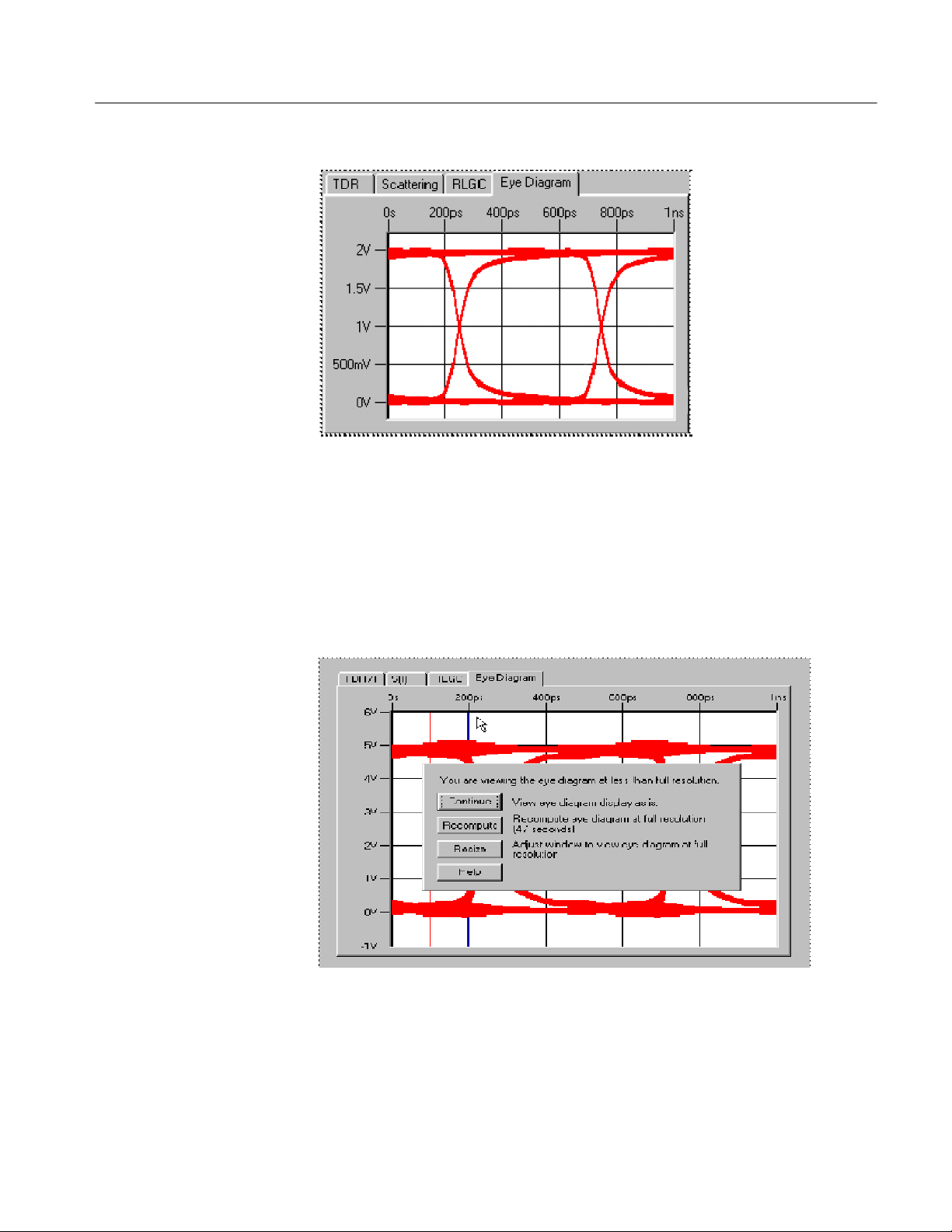
Figure 2- 25: Display the eye diagram

Operating Basics

Eye Diagram Zooming

When zooming in on an eye generated with long data sequences, you will be asked to choose the zoom method as shown in Figure 2--26. Choosing Continue is the fastest method, but you will be viewing the zoom area at less than full resolution. Choosing Recompute is the slowest but most accurate method. Choosing Resize will return you to the eye diagram you originally viewed.

Figure 2- 26: Choose the zoom method

When recomputing the eye diagram, if the computation takes too long, you can use the Cancel button to cancel the computation.

IConnectR and MeasureXtractort 4. 0 User Manual

2- 23

Operating Basics

Eye Masking Testing

You can set up your mask to perform electrical compliance testing with such standards as PCI Xpress, SATA, Infiniband, and XAUI.

As shown in Figure 2--27, you can select the appropriate polygon (2 is the main central polygon, 1 and 3 are the upper and lower polygons). The vertices of the eye mask can be moved by hand. Click Apply to apply the eye mask to existing eye, or Save to save the eye mask information into a file. Eye mask information can also be saved as part of a lossy line model.

Measure Jitter

Figure 2- 27: Select a polygon

Click Enable Eye Measurements at the bottom of the eye window shown in Figure 2--28, and you will be able to read eye width and height, as well as peak-to-peak jitter and amplitude noise. Amplitude noise can be read at the high or low levels. Note that interconnects generate only deterministic jitter, and there is no meaning for “RMS” jitter.

2- 24

IConnectR and MeasureXtractort 4. 0 User Manual

Figure 2- 28: Display the eye measurement s

Operating Basics

Correlation

In the eye diagram measurement for an interconnect, you characterize the deterministic jitter due to crosstalk and losses in the passive, linear interconnect system. As a result, TDR-based eye diagrams are the exact representation of the eye diagram degradation for the given interconnect. This is true as long as the measurement is performed with sufficient accuracy and care to characterize a given interconnect to a frequency that is at least 1.5/t

,wheretris the risetime of

the clock signal you will use to generate your eye.

Figure 2- 29: Directly measured eye diagram response

IConnectR and MeasureXtractort 4. 0 User Manual

2- 25

Operating Basics

Figure 2- 30: Eye diagram response from TDT measur ements

Eye Diagram Accuracy. Despite the simplicity of the TDR transmission eye

diagram measurement process, there are questions of accuracy. This tutorial compares eye diagram measurements in IConnect using a TDR oscilloscope transmission measurement with eye diagram measurements using a system based on a bit-error-rate tester or a pattern generator and a sampling oscilloscope.

Since this procedure characterizes only the deterministic jitter due to crosstalk and losses in the passive, linear interconnect system, a TDR-based eye diagram for the interconnect is effectively the exact representation of the eye diagram degradation for the given interconnect. As such, TDR-based eye diagram computation is correct by design.

To confirm this, the tutorial includes several examples of correlation of TDR-based eye diagram measurements to directly measured eye diagrams. As long as the TDR transmission measurement is performed with sufficient accuracy and care to characterize a given interconnect to a frequency that is at least 1.5/t

(where tris the risetime of the clock signal used to generate the eye

diagram), the eye diagram will be correct.

2- 26

IConnectR and MeasureXtractort 4. 0 User Manual

Operating Basics

System Eye Diagram

The eye diagram measured in IConnect shows signal degradation due to interconnect losses and crosstalk. In order to obtain a complete picture for the digital system eye diagram, the designer needs to extract the lossy coupled models for the interconnects in IConnect TDR and VNA software, and simulate propagation of the signal from a real digital I/O driver into these interconnect models in a simulator that has eye diagram display capability.

Board

Figure 2- 31: System used to measure and predict the eye diagram

S-Parameter Computation Tutorial

This tutorial guides you through the steps necessary to obtain the single ended or differential S-parameters and insertion and return loss for an interconnect from Time Domain Reflection (TDR) and Transmission (TDT) measurements. Frequency-domain scattering parameters are a useful way to visualize the electrical properties of a system. This tutorial leads you from a set of raw measurements to a complete set of S-parameters for your device under test (DUT), and allows you to evaluate the insertion and return loss of your device accurately, quickly, and efficiently.

Connector

Cable

Daughter card

Connector

Backplane

What are S-Parameters?

S-Parameters and TDR/T Data. Frequency-domain scattering parameters (S-parameters) are a useful way to visualize the electrical properties of a system. They are a dual representation of TDR and TDT data in the frequency domain. Although S-parameters have historically been measured in the frequency domain using a network analyzer, the same information is contained in TDR and TDT measurements.

Differential and mixed mode S-parameters can be obtained from corresponding TDR oscilloscope data. From a practical standpoint, TDR/T-based S-parameters are much simpler and quicker to obtain, while providing more than sufficient dynamic range. In addition, a designer who already has a TDR oscilloscope can save money by not buying a network analyzer, and using the TDR oscilloscope with IConnect TDR and VNA software instead.

IConnectR and MeasureXtractort 4. 0 User Manual

2- 27

Operating Basics

Waveform Acquisition and

Setup

BeginbyreviewingPreparing to Take Measurements on page 2--2 if necessary.

Acquisition Window. In addition to the best practices outlined in Preparing to T ake Measurements on page 2--2, for the S-parameter measurement it is

particularly important to select a window that is long enough to let the DUT waveform completely settle to its steady-state DC level. High-frequency analysis of the DUT requires that you let the signal settle to make an accurate analysis.

You also need to make sure that enough data points are selected in the oscilloscope acquisition window. This is particularly critical for analyzing long interconnects, such as cables. The upper frequency limit of your measurement is determined as:

window

upper

where N is the number of points in the acquisition window, t and t

window

is the acquisition window length. Thus, to get S-parameter data to the

desired upper frequency f

window

and f

upper

step

, you will need to make sure that the ratio between

window

is the time step,

step

the number of points and window length is sufficient.

To get the desired frequency step, you will need to make sure that the window length is sufficient. When working with long cables, it is generally a good idea to keep the number of points at the maximum number allowed for a given instrument. Furthermore, to increase the dynamic range of the measurements, it is important to keep the number of averages and number of points to the maximum, and the window as short as possible, as the equation below indicates:

2- 28

SNR(N, N

) = SNR(N0,N

avg

)·

Ꭹ

avg

avg0

Make sure to use heavy averaging in your instrument. Using 128 averages will give an extra 20dB or dynamic range; use at least that many if your instrument averages quickly. Keeping the acquisition window as short possible maximizes the effective power.

When dealing with differential measurements, you need to make sure that your signals arrive at the DUT at the same time. You can follow the deskew procedure in your oscilloscope manual, and having observed the difference in delays between the two channels in differential mode, adjust for half of that difference by using delta TDR function in the oscilloscope.

Tutorial Waveform Data. To follow our example, select Virtual Scope in the drop-down list at the top of the acquisition window. The Virtual Scope is a tool for loading waveforms from your hard drive using the same interface as that used for oscilloscopes.

IConnectR and MeasureXtractort 4. 0 User Manual

Operating Basics

Click the Instrument Settings tab at the top of the acquisition window to set the Virtual Scope options. Set the directory to C:\Program Files\TDA Sys-

tems\IConnect\Tutorials\Lossy Line. Set the filter to *.wfm, and click the Measure tab to begin taking measurements. Select the waveforms Reflection.wfm, Transmission.wfm,andOpen.wfm from the acquisition window.

Press the Acquire button, which opens up a new waveform viewer containing the two waveforms.

S- Parameter Data

Acquisition

To compute S-parameters, you need to obtain a reference and a DUT waveform.

The reference waveform de-embeds the cable, probe, and fixture from the measurement, and establishes a measurement reference plance. The reference waveform can be an open reference, acquired at the end of the cable, fixture, or probe interfacing your TDR instrument to the DUT. Alternatively, one can use a through measurement as a reference. Using through as a reference can be advantageous when a good reflected reference open cannot be achieved, or to better comply with certain measurement standard procedures, such as Serial ATA, Infiniband or PCI Xpress, which provide through structures on their fixtures for de-embedding the insertion loss of a fixture.

A DUT waveform can be any waveform measured from the DUT: forward reflection (TDR), forward transmission from channel 1 to channel 2 (TDT), backward reflection or backward transmission from channel 2 to channel 1 (in which case the signal is going to be launched from the second output of the TDR sampling head). The corresponding S-parameters will be S

(forward TDR), S

(forward TDT), S22(backward TDR) and S12(backward TDT). When measuring frequency domain crosstalk, just like in time domain, you would be measuring TDT to the adjacent channel, resulting in S

into an adjacent channel. Please

note that even if you are taking TDR (return loss) measurement, the far end of the device must be terminated with 50 Ω.

TDR stimulus on channel 1,

response on channel 1

TDR stimulus on channel 1,

response on channel 2

Figure 2- 32: Mapping between scattering parameters and TDR/T measurements

IConnectR and MeasureXtractort 4. 0 User Manual

TDR stimulus on channel 2,

response on channel 1

TDR stimulus on channel 2,

response on channel 2

2- 29

Operating Basics

DUT Connections

The TDR waveform in the S-parameter computation must be acquired with the 50 Ω cables connected to both DUT ports, thus ensuring a 50 Ω termination at the far end of the DUT. The cables, probes or fixtures used to connect the DUT to both channels of the TDR oscilloscope are assumed to be of the same length. In differential mode, both transmission and reference must be differential (that is, negative switching channel subtracted from the positive switching channel).

Reference measurement: Differential stimulus is ON on channels M1, M2. Reflection is measured on the same channels M1--M2

Fixture 1

Fixture 2

Reference and transmission on measurement:s Differential stimulus is ON on channels M1, M2. Transmission is measured on channels M3--M4 Reflection is measured on the same channels M1--M2

Fixture 1

DUT

Fixture 2

Differential, Common, and

Mixed Modes

Figure 2- 33: Measurement termination scheme

For a symmetric interconnect, you can use odd mode waveforms, acquired on the positive switching channel with the stimulus being in differential mode. Please note that even if you are only taking a TDR (return loss) measurement, the far end of the device must be terminated with 50 Ω on each port. 100 Ω differential termination is acceptable for differential response measurements.

For differential, common mode and mixed mode S-parameters, the same applies

- a reference and a DUT waveform are required. Before beginning the measurements, however, make sure to follow the procedure for your TDR instrument to align the TDR sources at the DUT measurement reference plane. For differential stimulus waveforms, the oscilloscope must have the two stimulus signals switching in opposite directions. For common mode stimulus waveforms, the oscilloscope must have the stimuli switching in the same direction. For differential response, subtract one response channel from the other. For the common mode response, add the two response channels together.

Differential S- Parameters. If the two lines in the differential pair are symmetric, stimulate the differential pair with a differential stimulus in the TDR oscilloscope (stimuli channels switching in the opposite direction), and acquire the waveform on the positive switching channel (Ch1). If you use a reference open

2- 30

IConnectR and MeasureXtractort 4. 0 User Manual

Operating Basics

waveform, you acquire it on the same channel, and use it to compute the differential S

(return loss).

For insertion loss, examine the transmission waveform on the positive switching channel (most likely Ch3). If you are using a transmission without the DUT in place as a reference, you will be acquiring it on the same channel.

Differential TDR stimulus, differential response

Figure 2- 34: Differential-Differential block of mixed mode S-Parameters

For a case of differential lines with mild asymmetry, proceed as follows: when the TDR is in differential mode, and the oscilloscope displays voltage, subtract the negative switching channel (Ch2) from the positive switching channel Ch1 (DUT = Ch1 - Ch2). Then, acquire reference on both channels simultaneously and subtract Ch1Ref - Ch2Ref again. Now, use the DUT waveform and the computed reference waveform to compute differential S

. Again, for insertion

loss, use the difference between positive and negative switching transmission channels (most likely Ch3 - Ch4). This latter procedure should always be used when acquiring data for frequency domain crosstalk computation.

Common Mode S- Parameters. The same discussion as for differential S-parameters applies, except the stimulus used must be a common mode stimulus (stimuli channels switching in the same direction). In addition, for traces with asymmetry, you will need to add the appropriate channels instead of subtracting them (reference is produced from Ch1Ref+Ch2Ref, common mode S from Ch1+Ch2, and common mode S Figure 2--35.

Common mode TDR stimulus, common mode response

Figure 2- 35: Common-Common block of mixed mode S-Parameters

IConnectR and MeasureXtractort 4. 0 User Manual

or return loss

or insertion loss from Ch3+Ch4). See

2- 31

Operating Basics

Mixed Mode S- Parameters. Mode conversion parameters are much less important, but if you need to obtain them, proceed using the same process as for common mode S parameters, except for the following. For differential-to-common mode conversion the stimulus is differential, whereas the acquisition is performed only using the sum of the channels (reference is produced from Ch1ref-Ch2ref, differential-to-common mode conversion S differential-to-common mode conversion S

or return loss from Ch1+Ch2, and

or insertion loss from Ch3+Ch4).

For common mode to differential mode conversion, the stimulus is common mode, whereas the acquisition is performed using only the difference between the channels.

Normally, the differential-to-common mode differences should be 0 across the acquisition window; when there is skew, however, they will be non-zero and will produce non-zero frequency dependent mode conversion.

Mixed mode

Compute S- Parameters

Figure 2- 36: Mode Conversion block of mixed mode S-Param eters

If the Compute window is not visible, select S-Parameter from the Compute menu. The scattering parameter is computed from the computation window by choosing S-Parameter from the Compute list box as shown in Figure 2--37, or by clicking on the separate ‘S’ button on the toolbar. From the drop-down list box titled Ref:, choose your reference waveform.

2- 32

IConnectR and MeasureXtractort 4. 0 User Manual

Figure 2- 37: Computing S-Parameter

Operating Basics

S- Parameter Options

From the list box titled DUT: choose the measured response of the DUT to the input step. Click the Compute button, and a new frequency-domain waveform viewer will be created with the scattering response in it.

Additional options are available when computing S-Parameters, as shown in Figure 2--38. First, you can let IConnect determine the highest frequency content of the data, or you can check the Set Manually check box and enter the desired delta_f and F_upper values. Furthermore, you can choose to perform a 50 Ω calibration, using a precision 50 Ω standard at the DUT reference plane. You also have a choice between open, short, and through reference.

NOTE. The 50 Ω calibration waveform is ignored for insertion loss/crosstalk measurements if a through reference is used.

IConnectR and MeasureXtractort 4. 0 User Manual

2- 33

Operating Basics

Calibration

Choosing the Data Display

Figure 2- 38: S-Parameter fields in the Computation dialog box

Calibration methods are often used to remove the effects of the fixturing used to measure the DUT. The calibration implemented in IConnect is a short version of a standard S-O-L-T (Short-Open-Load-Thru calibration), which provides sufficient accuracy for digital signal integrity measurements and digital design electrical compliance tests. It is critical to remember, however, that the accuracy benefits that calibration provides only manifest themselves when high-quality calibration standards are used, and when the measurement repeatability is ensured. Measurement repeatability is always important to improving accuracy.

It should be noted that for most signal integrity and digital design tasks, good measurements could be obtained even without calibration, if quality cables and connectors are used.

Note that since the tutorial uses a forward TDT (transmission) waveform of the DUT, the resulting S-parameter is S

(insertion loss). If you use a TDR

(reflection waveform), you will obtain return loss; if you use TDT into the adjacent line, you will obtain crosstalk in frequency domain.

2- 34

IConnectR and MeasureXtractort 4. 0 User Manual

Operating Basics

Right-click in the frequency domain waveform viewer, select Plot, and choose the desired format for the S-parameter display as shown in Figure 2--39. The most common display in signal integrity is dB(Mag)/Phase. Right-click on the displayed waveform, and select Cursor Readout to view the values.

Differential Example

Figure 2- 39: Single-ended S21data computed from TDT measurement

Figure 2--40 is an example of differential return loss (S

parameter) in

11dd

IConnect. Right-click in the frequency domain waveform viewer, select Plot,and choose the desired format for the S-parameter display. The most common display in signal integrity is dB(Mag)/Phase. Right-click on the displayed waveform, and turn on cursor readout to view the values.

IConnectR and MeasureXtractort 4. 0 User Manual

2- 35

Operating Basics

Figure 2- 40: Differential S-Parameter example

S- Parameter Window. Please note that the S-parameters can also be computed by

opening any of the modeling windows (for example, the lossy line modeling window, as shown in Figure 2--41 ), loading the appropriate data, and clicking on the S(f) tab as shown in Figure 2--41. The S (f) tab lets you view your measurements and model response in the frequency domain.

2- 36

Figure 2- 41: The S(f) tab

IConnectR and MeasureXtractort 4. 0 User Manual

Operating Basics

Exporting Touchstone

You can export the data in your comma-separated values (csv) or Touchstone format, Touchstone being the standard S-parameter interchange format, using the File/Export menu as shown in Figure 2--42. You can export 1-port, 2-port, 4-port single-ended and 4-port differential S -parameters.

Figure 2- 42: Exporting Touchstone data

Exporting S2P and S4P. You will need at least three waveforms in your frequency

domain viewer to export a 2-port Touchstone file if your DUT is reciprocal (S21 = S12). You will need four waveforms if it is non-reciprocal.

Figure 2- 43: Export a 2-port Touchstone file

You will need at least 10 waveforms to export a 4-port Touchstone file if your DUT is reciprocal, and 16 waveforms if it is not.

IConnectR and MeasureXtractort 4. 0 User Manual

2- 37

Operating Basics

Figure 2- 44: Export a 4-port Touchstone file

Most interconnect networks are reciprocal.

Correlation

Figure 2--45 provides an excellent illustration of correlation between a TDRbased insertion loss computed in IConnect and a VNA insertion loss up to 12 GHz.

Figure 2- 45: Correlation example

2- 38

IConnectR and MeasureXtractort 4. 0 User Manual

Lumped LC Computation Tutorial

This tutorial guides you through the steps to obtain accurate inductance and capacitance measurements. This is a relative measurement technique, which is based on two comparative measurements with and without the Device Under Test (DUT) in place, and is based on the JEDEC document JEP-123 and the IBIS standard for measuring L and C. The tutorial leads you from a set of raw measurements to accurately measured L and C values, and enables you to evaluate the model and verify its accuracy.

This technique can be used to measure the inductance or capacitance of a package, connector, via, or an active device I/O buffer capacitance.

Validity of L and C Models. The JEDEC and IBIS standard techniques for L and C computation described here are only valid if your DUT is electrically short compared to the rise time of the signals propagating through it (t the device is not electrically short, the DUT cannot be described using a simple lumped or lumped coupled model, whether obtained through the techniques described here or any other time or frequency domain measurement technique. A distributed model, based on the impedance profile computed in IConnect, must be used instead, or the DUT must be split into shorter subsegments, each such subsegment shorter than the signal rise time. For practical purposes, the electrical length of the DUT must be 2 to 3 times shorter than the rise time of the signals.

Operating Basics

dut

<< t

rise

). If

Waveform Acquisition and

Setup

ref short

TDR

ref open

TDR

Figure 2- 46: Computation of L and C

BeginbyreviewingPreparing to Take Measurements on page 2--2 if necessary. For LC measurements, it is particularly important to select a window that is long enough to allow the DUT waveform to completely settle to its steady state DC level. Since you are performing a steady-state analysis of the DUT, you need to allow the signal to settle to make this analysis accurately.

The asymptotic capacitance and inductance computation are accessed via the computation window, from the Compute menu, as shown in Figure 2--47. The computation to be performed is chosen from the computation drop-down, which causes the drop-down list boxes and their labels in the Waveforms group to

IConnectR and MeasureXtractort 4. 0 User Manual

2- 39

Operating Basics

adjust for data entry. It may be necessary to choose a waveform viewer from which to choose the input waveforms for the computation. This viewer also receives the resulting waveform once it is computed.

Figure 2- 47: Choosing self inductance computation from the main menu

Measurement Setup Tips

To follow our example, select Virtual Scope in the drop-down list at the top of the acquisition window. The virtual scope is a tool for loading waveforms from your hard drive using the same interface as that used for oscilloscopes. Press the Instrument Settings tab at the top of the acquisition window to set the Virtual Scope options. Set the directory to Tutorials\I/O Buffer Capacitance, under the IConnect installation directory, C:\Program Files\TDA Systems\IConnect\.Set the filter to *.wfm, and press the Measure tab to begin taking measurements.

Select the waveforms Fixture_open.wfm and DUT_open.wfm from the acquisition window. These are the waveforms with the ATE fixture and socket for the given device with and without the actual device in the socket. Press the Acquire button, which opens up a new waveform viewer containing the two waveforms.

Wait for steady state. Each of these methods is based on the DC relationships between charge and voltage (capacitance) and flux and current (inductance). For this reason, it is necessary that all waveforms reach a steady state value in order to get accurate results.

2- 40

Use the correct reference waveform. Parasitic measurements require information

on what the ideal response would be - open circuit for self capacitance, or short circuit for self inductance. Mutual measurements require only input information to determine the initial and final voltage and values.

IConnectR and MeasureXtractort 4. 0 User Manual

Operating Basics

Pay attention to quiescent nearby leads or lines. Also pay attention to the far ends of the lines under test. For capacitance measurements, the lead(s) in question should be open-circuited at the far end, and adjacent leads short-circuited to ground. For inductance measurements, this arrangement is reversed.

Self Inductance

In the computation window, choose L-Self as your computation, as shown in Figure 2--48. In the DUT: waveform chooser, select the measurement of your DUT short-circuited at the far end. For the Short: waveform chooser, select the reference waveform that corresponds to your measurement system shorted where the DUT would normally be placed. It may be necessary to enter the characteristic impedance and step amplitude for your measurement system before performing the computation, or change the step amplitude to the correct value.

Once these parameters have been chosen, pressing the Compute button performs the computation.

The resultant waveform will be placed in the chosen waveform viewer and the inductance is measured as the final asymptotic level that the inductance waveform reaches. If the cursors are used to make the measurement, they read directly in units of Henries.

IConnectR and MeasureXtractort 4. 0 User Manual

2- 41

Operating Basics

2- 42

Self Capacitance

Figure 2- 48: Displaying a self inductance measur ement

In the computation window, choose C-Self as your computation, as shown in Figure 2--49. In the DUT: waveform chooser, select the measurement of the DUT open-circuited at the far end. In the Open: waveform option, select the reference waveform, which corresponds to the measurement system open-circuited where the DUT would normally be placed.

It may be necessary to enter the characteristic impedance and step amplitude for your measurement system prior to performing the computation, or change the step amplitude to the correct value. Once these parameters have been chosen, pressing the Compute button performs the computation.

The resultant waveform will be placed in the chosen waveform viewer, and the capacitance is typically measured as the final asymptotic level that the capacitance waveform reaches. If the cursors are used to make the measurement, they read directly in units of Farads.

IConnectR and MeasureXtractort 4. 0 User Manual

Operating Basics

Figure 2- 49: Displaying a self capacitance measur ement

Mutual Inductance

IConnectR and MeasureXtractort 4. 0 User Manual

In the computation window, choose L-Mutual as your computation, as shown in Figure 2--50. In the DUT: waveform option, select the measurement of the near-side crosstalk on the quiescent line with adjacent leads open at the near end, short-circuited at the far end. In the Short: waveform chooser, s elect the waveform that corresponds to your measurement system shorted where the DUT would normally be placed. In the Background: waveform option, select the background waveform, which is acquired on the channel used to measure the DUT waveform when the DUT is disconnected.

It may be necessary to enter the characteristic impedance and step amplitude for your measurement system prior to performing the computation.

2- 43

Operating Basics

Once the above parameters have been chosen, pressing the Compute button performs the computation. The resultant waveform will be placed in the chosen waveform viewer, and the inductance is typically measured as the final asymptotic level that the inductance waveform reaches. If the cursors are used to make the measurement, they read directly in units of Henries.

2- 44

Mutual Capacitance

Figure 2- 50: Displaying a mutual inductance m easurement

In the computation window, choose C-Mutual as your computation, as shown in Figure 2--51. In the DUT: waveform option, select the measurement of the near-side crosstalk on the quiescent line with adjacent leads shorted at the near end, open-circuited at the far end.

In the Open: waveform choice, select the waveform that corresponds to your measurement system open-circuited, where the DUT would normally be placed. In the Background: waveform option, select the background waveform, which

IConnectR and MeasureXtractort 4. 0 User Manual

Operating Basics

is acquired on the channel used to measure the DUT waveform when the DUT is disconnected.

It may be necessary to enter the characteristic impedance and step amplitude for your measurement system prior to performing the computation. Once the above parameters have been chosen, pressing the Compute button performs the computation. The resultant waveform will be placed in the chosen waveform viewer, and the capacitance is typically measured as the final asymptotic level that the waveform reaches. If the cursors are used to make the measurement, they read directly in units of Farads.

Figure 2- 51: Displaying a mutual capacitance m easurement

IConnectR and MeasureXtractort 4. 0 User Manual

2- 45

Operating Basics

I/O Buffer Input

Capacitance

As shown in Figure 2--52, In the DUT: waveform chooser, select the DUT_open.wfm, the waveform of the fixture with the packaged part inside the

socket. In the Open: waveform option, select fixture_open.wfm, the waveform of the fixture without the part inside the socket.

Follow the same procedure as for general C-Self for computation of input die capacitance. In the computation window, choose C-Self as your computation.

It may be necessary to enter the characteristic impedance and step amplitude for your measurement system prior to performing the computation, or change the step amplitude to the correct value.

Once these parameters have been chosen, pressing the Compute button performs the computation. The resultant waveform will be placed in the chosen waveform viewer, and the capacitance is typically measured as the final asymptotic level that the capacitance waveform reaches. If the cursors are used to make the measurement, they read directly in units of Farads. In this case, the reading is

4.6 pF.

2- 46

Simulate

Read I/O buffer

capacitance value

Figure 2- 52: Extracting I/O buff er capacitance

Even though the computational methods described above are standardized by JEDEC and the IBIS Accuracy Standard, it is important to verify the accuracy of the computed values by running a simulation and comparing it against a measurement. Use either a Lumped or Lumped Coupled model, as shown in Figure 2--53, for the device model, depending on whether you are required or not required to compute mutual parameters and crosstalk.

IConnectR and MeasureXtractort 4. 0 User Manual

Operating Basics

Set up a new Composite model viewer, add a TDR source, device model and termination, and run a simulation to validate the model. For more information on running a simulation and validating a model in IConnect, refer to Simulation on page 6--1.

Figure 2- 53: IConnect lumped model editor

Figure 2- 54: IConnect lumped coupled model editor

IConnectR and MeasureXtractort 4. 0 User Manual

2- 47

Operating Basics

Single and Coupled Line Modeling Tutorial

This tutorial guides you through the steps necessary to obtain single and coupled lossless transmission line model in IConnect. The single and coupled transmission line model allows you to simulate the reflections, ringing and crosstalk in your interconnects, and is useful for short transmission line segments, electrically long packages and connectors, single-ended, differential, and coupled.

This tutorial leads you from a set of raw measurements to a complete SPICE model, and allows you to evaluate the model and verify its accuracy. Should you have additional questions about this tutorial, see Single Line on page 5--9 or Symmetric Coupled Lossy Lines on page 5--29 in the IConnect reference manual, or contact us to get more information through our technical support.

Single- Ended and Differential TDR. Single-ended and differential TDR modeling techniques allow you to extract accurate transmission line impedance for the traces on the board, differential and coupled transmission line models, as well as self and mutual inductances and capacitances of vias and other lumped components in the system. The same techniques are applicable for characterization of package, socket, connector and cable interconnects that are electrically long. The interconnect is electrically long when the rise time of the signals propagating through these interconnects is much longer than the electrical length of the interconnect.

Waveform Acquisition and

Setup

You should begin by reviewing Preparing to Take Measurements on page 2--2 if necessary. It contains useful information on setting up your instrument to communicate with IConnect, as well as suggestions for taking good measurements.

A Single Line window can be created either from the Model/Single Line menu item, or by using the Single Line button on the Model Toolbar. The Symmetric Coupled Line Model can be launched from the Model/Symmetric Coupled menu item, or by using the Symmetric Coupled button on the Model Toolbar.

2- 48

IConnectR and MeasureXtractort 4. 0 User Manual

Single line model

Operating Basics

Coupled line model

DUT Connections

Figure 2- 55: Creating a Single Line or Symm etric Coupled Lines model

In differential or common mode, both transmission and reference measurements must be differential (the negative switching channel is subtracted from the positive switching channel) or common mode (the two positive switching channels are added together).

It is important to de-skew the TDR oscilloscope channels while doing differential measurements. Follow your oscilloscope de-skewing procedure before acquiring differential data.

IConnectR and MeasureXtractort 4. 0 User Manual

2- 49

Operating Basics

Loading Data

Reference measurement: Differential stimulus is ON on channels M1, M2. Reflection is measured on the same channels M1--M2

Fixture 1

Fixture 2

Reference and transmission on measurement:s Differential stimulus is ON on channels M1, M2. Transmission is measured on channels M3--M4 Reflection is measured on the same channels M1--M2

Fixture 1

DUT

Fixture 2

Figure 2- 56: DUT setup for differential reference, reflection, and transmission

Two waveforms will be required for single line modeling - a reference open waveform and a reflection waveform. In the case of a symmetric coupled line model, the two reflection waveforms must be acquired - in odd mode and even mode configurations.

Read the waveform descriptions in the Load Reference Waveform dialog box, shown in Figure 2--57, to capture a proper waveform from the instrument. The tutorial waveforms, named Open.wfm and DUT.wfm, can be found in the Tutorials\Single Line directory under the IConnect installation directory.

2- 50

Figure 2- 57: The Load Reference Waveform dialog box

IConnectR and MeasureXtractort 4. 0 User Manual

Reference

Reflection

Operating Basics

Load data

Computing Z- Line

Figure 2- 58: Loading reference and reflection waveforms into the single line model

Now make sure that the type of termination selected in the Termination Type drop-down box matches the actual termination at the end of your DUT. If your interconnect DUT terminates into a high-impedance I/O buffer, choose Open termination type, since a simple model for such buffer consists of an input buffer capacitance and an open termination.

Click Compute and the impedance profile (Z-line) is computed and displayed in the Partitions window. In the case of the symmetric coupled lines model, you will have two impedance profiles - Odd and Even - displayed simultaneously. To learn more about impedance profile computation, see the True Impedance Profile (Z--Line) Computation Tutorial on page 2--6 or Impedance Profile Computation on page 9--4.

IConnectR and MeasureXtractort 4. 0 User Manual

2- 51

Operating Basics

Reference

Load data

Reflection

Windowing the Data

Figure 2- 59: Compute the impedance profile by pressing the Compute button

ClickontheModel tab. Select the green cursor on the left, and move it to the beginning of the waveform response, which occurs around 250 ps. Select the green cursor on the right, and move it to the end of the waveform response, which occurs around 2.5 ns. By placing these two cursors, you are windowing out the portions of the waveform (covered by yellow) that correspond to the measurement setup rather than to the DUT itself.

2- 52

IConnectR and MeasureXtractort 4. 0 User Manual

Operating Basics

Partitioning Details

Figure 2- 60: Windowing out the part of the response you don’t want to model

Even though IConnect automatically partitions the waveform, it is important to know how to place these partitions (to know where one line begins and the other one ends) in case you need to adjust the partitions placed by IConnect. When the TDR step propagates through the interconnect, the TDR waveform stays at a steady level. As soon as it sees the next transmission line with a different impedance in its path, it begins to change. Therefore, you place the partitions where the waveform begins to change.

The same rule applies to transmission lines and lumped elements (capacitances and inductances) since a capacitance or an inductance is just a very short piece of transmission line. Typically, you partition at the peaks of lumped elements, and select Mean value computation from the Impedance drop down box.

You can zoom in the Partitions window by holding down Control-Shift while dragging out the zoom area with your mouse.

IConnectR and MeasureXtractort 4. 0 User Manual

2- 53

Operating Basics

Other Practical Details

As a general rule, partitions can be created at the right edge of a segment of fairly constant impedance, and the impedance value assigned using the Right Edge criteria. This approach results in accurate models for many types of structures. However, your choice of partition size and type should be based on your own judgment to achieve a simple model which is accurate enough for your needs.

Remember, a transmission line of delay T resolve it. In other words, any segment with T where T

is the risetime of the target system in which the model will be used.

requires a risetime less than 2Tdto

/2 need not be modeled,

d<Tr

Each of the partitions uses T-Li ne topology with a single segment. Note that additional RLGC topologies are available for other modeling applications.

Symmetric Coupled Model

Details

Figure 2- 61: Single line partitioning exam ples

The files for this symmetric coupled line modeling example are found in the directory Tutorials/Coupled Lines under the IConnect installation directory. Open the Symmetric Coupled Line modeling window, and load the required even (even.wfm), odd (odd.wfm) and reference (short,wfm) waveforms using the appropriate buttons under the Measure tab. Click the Compute button, and use the same partitioning procedure as that for the Single Line model.

For our symmetric coupled line example, it may be instructive to note that the physical structure from which the measurements were taken was a set of two coupled lines, which diverged to SMA connectors at either end. From this knowledge, you would expect to see, qualitatively speaking, a coupled section in the middle of the model, and two short uncoupled sections at either end.

The question remains, however, as to the degree of coupling and the lengths of the coupled and uncoupled segments. The leftmost partition can be seen to be uncoupled, since the even- and odd-mode responses are the same. To inform IConnect of this fact, select the leftmost partition and uncheck the Coupled checkbox. Its edge is where the even- and odd-mode impedance profiles begin to diverge.

2- 54

IConnectR and MeasureXtractort 4. 0 User Manual

Operating Basics

Figure 2- 62: Partitioning the first, uncoupled segment

The second partition, highlighted in blue, is obviously coupled, since the evenand odd-mode impedances are different from each other . If this partition is highlighted and the Coupled check-box is checked, a second dotted odd-mode partition divider should appear within the selected partition.

IConnectR and MeasureXtractort 4. 0 User Manual

2- 55

Operating Basics

Figure 2- 63: Partitioning the second, coupled segment

Saving the Model

The purpose of this odd-mode divider is to mark where the odd impedance changes. The edge of the even divider should be at the right edge of the uniform impedance segment in the even-mode (red) waveform, and the edge of the odd (dotted) divider should be at the edge of the uniform segment in the odd-mode (green) waveform. If the odd-mode divider turns red when you move it, you have moved it to a position in which the model parameters preclude being able to build a passive model, which could result in simulation stability problems. The divider must be moved, or the parameters manually adjusted, before the model can be saved.

You are returning to the Single Line modeling example.

Save the Single Line model to a meaningful name, such as Single Line.cir,in the Single Line directory. This may be done via the File/Save command, from the standard toolbar, by using the <Ctrl+S> keyboard shortcut, or by right-clicking in the model window and choosing Save from the resultant context menu. Make sure to select the appropriate SPICE output format when saving the model.

2- 56

IConnectR and MeasureXtractort 4. 0 User Manual

Figure 2- 64: Saving the single line model

Operating Basics

Viewing the Model. The easiest way to view the saved model is to right click in the modeling window and click View Netlist.

Figure 2- 65: Use the context menu to quickly view the model netlist

Simulating

IConnectR and MeasureXtractort 4. 0 User Manual

Click the Simulate tab, and then click Simulate to automatically generate the model and simulate it in your simulator of choice. You can choose a link to your preferred simulator in Tools/Options/Simulator Options. Make sure that your selected file format matches your simulator selection.

2- 57

Operating Basics

Figure 2- 66: The Simulate button

The Composite model, including the piecewise linear TDR source, single line model and termination, is generated automatically. You can double-click any of the composite model elements to view the included models. In the case of a symmetric coupled lines model, two composite models will be generated, to validate the accuracy for both even and odd modes of propagation.

2- 58

PWL Source

Figure 2- 67: Composite model with the DUT submodel, a source to drive it, and a resistance to terminate it

If you believe that you need to increase the precision with which IConnect models the TDR source, decrease the Max Error settings and click Partition to repartition the model. Make sure to save it before continuing. To reverse the polarity of the TDR source, change the sign in the Scale box, in the Model group box.

IConnectR and MeasureXtractort 4. 0 User Manual

Figure 2- 68: You can edit the automatically generated PWL source

Operating Basics

Analyzing the Results

After the simulation is complete, the simulated waveforms are placed in the composite model waveform viewer. Click on the TDR/T or S(f) tabs to observe the correlation. As you can observe, even without modeling the losses, the correlation is very good. However, to be absolutely certain of the accuracy of the model, you are advised to achieve correlation for both reflection and transmission waveforms. If the match is satisfactory, then the modeling session is done. If it is not, it may be necessary to return to the various model editors, alter the models, and resimulate.

If the waveforms are offset on the screen, drag one of them with the mouse to overlay on top of the other. In the case of a symmetric coupled line model, the match for both even and odd mode waveforms must be ensured.

IConnectR and MeasureXtractort 4. 0 User Manual

2- 59

Operating Basics

Figure 2- 69: Viewing correlation in the Composite model viewer

Risetime Filtering

In most cases the model you are creating will be used in a system whose risetime is slower than the 30-40 ps risetime of the TDR measurement head. In that case, it makes sense to filter the waveforms prior to comparison to see how both measurement and simulation would compare at a lower risetime. The lower risetime will correspond better to the fast corner of the actual drivers used in the system with the given interconnect under test.

To filter multiple waveforms, choose Filter Waveform from the Compute drop-down list. Type the desired risetime in the text box labeled Risetime at the bottom of the Computation Window. Select the waveforms to be filtered, right click on a selected waveform, and choose Filter from the menu.

The correlation at the actual device rise time is more important than the correlation at the TDR rise time.

Lossy Line Modeling Tutorial

This tutorial guides you through the steps to obtain a lossy transmission line model and eye diagram. The lossy transmission line model allows you to simulate the frequency dependent skin effect and dielectric losses for your interconnects, and is useful for single line and balanced differential line modeling (the latter in the odd mode configuration), as well as predicting the eye diagram degradation due to losses. The symmetric coupled lossy lines model allows you to simulate the skin effect and dielectric loss, together with the intersymbol interference (ISI) and crosstalk effects.

2- 60

IConnectR and MeasureXtractort 4. 0 User Manual

Operating Basics

It also allows you to predict the eye diagram degradation due to losses and ISI in the interconnects. This tutorial leads you from a set of raw measurements to a complete SPICE model, and allows you to evaluate the model and verify its accuracy. Should you have additional questions about this tutorial, see Lossy Line on page 5--21, or contact Tektronix to get more information through our technical support.

Waveform Acquisition and

Setup

You should begin by reviewing Preparing to Take Measurements on page 2--2 if necessary.

In addition to the best measurement practices described in Preparing to Take Measurements on page 2--2, it is particularly important for lossy line and eye diagram measurement to select a window that is long to allow the DUT waveforms to completely settle to their steady state DC levels. High-frequency DUT analysis requires that the signal completely settle to make an accurate analysis.

Lossy Line

Figure 2- 70: Creating a lossy line model via the Model menu or Model toolbar

A Lossy Line model can be created either from the Model/Lossy Line menu item, or by using the Lossy Line button on the Model Toolbar. A Symmetric Coupled Lossy Lines model can be launched from the Model/Symmetric Coupled Lossy Line, or using the Symmetric Coupled Lossy Line button on the Model toolbar.

IConnectR and MeasureXtractort 4. 0 User Manual

2- 61

Operating Basics

Note that losses are a characteristic of the interconnect material. Therefore, to get the best results, it is important to extract the losses on a transmission line of controlled impedance. It is possible to extract the losses based on structure with changing impedance, but if changes are very large, it will be difficult to extract losses accurately.

Choosing the Extract

Termination Type

You can select the Matched load in the Measure tab on the right of the IConnect window. This termination type will provide lossy transmission line data based on the TDT (Time Domain Transmission) measurement, with the far end of the device terminated in 50 Ω. You can also use the Open termination type, based on TDR (reflection) waveforms, in case TDT is difficult to perform (such as when the far end of the device is inaccessible). However, the transmission measurement is generally more accurate.

Select termination type

2- 62

DUT Connections

Figure 2- 71: Choosing a termination type for the Lossy Line model

IConnectR and MeasureXtractort 4. 0 User Manual

Operating Basics

It is important to de-skew the TDR oscilloscope channels while doing differential measurements. Follow your oscilloscope de-skewing procedure before acquiring differential data.

Loading Data

Reference measurement: Differential stimulus is ON on channels M1, M2. Reflection is measured on the same channels M1--M2

Fixture 1

Fixture 2

Reference and transmission on measurement:s Differential stimulus is ON on channels M1, M2. Transmission is measured on channels M3--M4 Reflection is measured on the same channels M1--M2

Fixture 1

DUT

Fixture 2

Figure 2- 72: DUTsetup for differential reference, reflection, and transmission

Now you can acquire the three required waveforms for matched-load lossy line modeling: Reference, Reflection, and Transmission. First, make sure to select the appropriate instrument in the Acquisition window. Click the button for each waveform in the Measure tab, and acquire the appropriate waveform from the instrument.

Reference Reflection

Figure 2- 73: Each waveform is loaded by clicking on its respective button

IConnectR and MeasureXtractort 4. 0 User Manual

Load data

Transmission

2- 63

Operating Basics

For symmetric lossy coupled lines, click on the Even Mode radio button, and acquire the two additional waveforms in the even mode.

TDR/T waveforms in the Matched termination extraction must be acquired with 50 Ω cables connected to both DUT ports, thus ensuring a 50 Ω termination at the far end of the DUT. The cables, probes and fixtures used to connect the DUT to both channels of the TDR oscilloscope are assumed by IConnect to be of the same length.

Three waveforms will be required for single lossy line modeling - a reference open waveform, and TDR and TDT waveforms. In the case of a symmetric coupled lossy lines model, these three waveforms must be acquired in odd mode configuration. In addition to the three odd mode waveforms, two waveforms for the even mode measurements will be required. Read the waveform descriptions in the Loard Reference Waveform dialog box, shown in Figure 2 -- 74, to capture a proper waveform from the instrument. The three tutorial waveforms, named

Reference.wfm, Reflection.wfm,andTransmission.wfm, can be found in the Tutorials\Lossy Line directory under the IConnect Installation directory.

2- 64

Model Extraction

Figure 2- 74: Load Reference Waveform dialog box

Once the data is loaded, click the Model tab. Click Compute in the Optimization group to extract the lossy line mode. If you know any of the parameters, you

can fix them during the optimization by checking the Fix box for the given parameter. In fact, it may be preferrableto extract the DC resistance of the interconnect beforehand, using a DC meter, and fix it during optimization.

IConnectR and MeasureXtractort 4. 0 User Manual

Operating Basics

During the optimization, the text of the Compute button changes to Cancel,and the number of iterations performed is continuously displayed. After the maximum number of iterations is reached, or the desired resolution is achieved, the computation stops, and the results of a simulation based on the newly extracted model are displayed in the TDR/T tab.

Model Accuracy

Figure 2- 75: The Optimize button

NOTE. The Optomize button is labeled Cancel when an extraction is running.

The correlation between the simulated (red) and measured data (black) in time domain is the key to accuracy of the extracted model. You can, however, also observe the correlation in frequency domain by clicking the S(f) tab. You can extract a better accuracy model, with correlation in both the time and frequency domains, by increasing the precision and the number of iterations in the optimization Options, or by changing the values manually and clicking the Evaluate button. Keep in mind that in digital design, time domain correlation is much more important than frequency domain correlation.

IConnectR and MeasureXtractort 4. 0 User Manual

2- 65

Operating Basics

Figure 2- 76: Lossy line model correlation in the frequency domain

Other Practical Details

You can also repeatedly click the Optimize button. The values may change slightly, but the new values will still give you an accurate model within the specified Precision parameter, accessible from the optimization Options button.

You can create test scenarios by changing any of the parameters manually, and clicking the Evaluate button. The new values will be evaluated and the new simulated waveform will be shown in red. Note that if the red waveform does not change substantially as you change the values in the window, this implies that your changes are not significant enough, or that the given loss mechanism is too small to matter.

2- 66

Change the value

Reevaluate

Figure 2- 77: Lossy line response to altering its optimized parameter values

IConnectR and MeasureXtractort 4. 0 User Manual

Tektronix IConnect,MeasureXtractor User Manual

Specifications and Main Features

Frequently Asked Questions

User Manual

Warranty 9(b)

Table of Contents

List of Figures

List of Tables

Getting Started

IConnect Overview

What You Can Do With IConnect

IConnect Installation Notes

Adobe Acrobat Reader

Manual Sentinel Hardware Key Driver Installation, Removal, and Configuration

Getting Started With IConnect

IConnect Shortcuts

Enhancements and Improvements in IConnect 4.0

Enhancements and Improvements in IConnect 3.6

Operating Basics

Preparing to Take Measurements

True Impedance Profile (Z -Line) Computation Tutorial

Eye Diagram Tutorial

S-Parameter Computation Tutorial

Lumped LC Computation Tutorial

Single and Coupled Line Modeling Tutorial

Lossy Line Modeling Tutorial