Tektronix Fundamentals Of Real-Time Spectrum Analysis User Manual

Fundamentals of Real-Time Spectrum Analysis

Primer

Table of Contents

Chapter 1: Introduction and Overview . . . . . . . . . . . . . . . . . . . . . . . . . . . . . . . . . . . . . . . . . . . . . . . . . . . . . . . . . . . . . . . . . . . . 2

The Evolution of RF Signals . . . . . . . . . . . . . . . . . . . . . . . . . . . . . . . . . . . . . . . . . . . . . . . . . . . . . . . . . . . . . . . . . . . . . . . . . . . . 2

Modern RF Measurement Challenges . . . . . . . . . . . . . . . . . . . . . . . . . . . . . . . . . . . . . . . . . . . . . . . . . . . . . . . . . . . . . . . . . . . . . 2

A Brief Survey of Instrument Architectures . . . . . . . . . . . . . . . . . . . . . . . . . . . . . . . . . . . . . . . . . . . . . . . . . . . . . . . . . . . . . . . . . . 3

Swept Spectrum Analyzers:

Traditional Frequency Domain Analysis . . . . . . . . . . . . . . . . . . . . . . . . . . . . . . . . . . . . . . . . . . . . . . . . . . . . . . . . . . . . . . . . . 3

Vector Signal Analyzers: Digital Modulation Analysis . . . . . . . . . . . . . . . . . . . . . . . . . . . . . . . . . . . . . . . . . . . . . . . . . . . . . . . . . . 4

Real-Time Spectrum Analyzers: Trigger, Capture, Analyze . . . . . . . . . . . . . . . . . . . . . . . . . . . . . . . . . . . . . . . . . . . . . . . . . . . . . . 4

Key Concepts of Real-Time Spectrum Analysis . . . . . . . . . . . . . . . . . . . . . . . . . . . . . . . . . . . . . . . . . . . . . . . . . . . . . . . . . . . . . . . 5

Samples, Frames, and Blocks . . . . . . . . . . . . . . . . . . . . . . . . . . . . . . . . . . . . . . . . . . . . . . . . . . . . . . . . . . . . . . . . . . . . . . . . . 5

Real-Time Triggering . . . . . . . . . . . . . . . . . . . . . . . . . . . . . . . . . . . . . . . . . . . . . . . . . . . . . . . . . . . . . . . . . . . . . . . . . . . . . . . 6

Seamless Capture and Spectrogram . . . . . . . . . . . . . . . . . . . . . . . . . . . . . . . . . . . . . . . . . . . . . . . . . . . . . . . . . . . . . . . . . . . . 7

Time-Correlated Multi-Domain Analysis . . . . . . . . . . . . . . . . . . . . . . . . . . . . . . . . . . . . . . . . . . . . . . . . . . . . . . . . . . . . . . . . . . 7

Chapter 2: How a Real-Time Spectrum Analyzer Works . . . . . . . . . . . . . . . . . . . . . . . . . . . . . . . . . . . . . . . . . . . . . . . . . . . . . . . 10

Digital Signal Processing in Real-Time Spectrum Analyzers. . . . . . . . . . . . . . . . . . . . . . . . . . . . . . . . . . . . . . . . . . . . . . . . . . . . . . 10

IF Digitizer . . . . . . . . . . . . . . . . . . . . . . . . . . . . . . . . . . . . . . . . . . . . . . . . . . . . . . . . . . . . . . . . . . . . . . . . . . . . . . . . . . . . . 10

Digital Down-Converter . . . . . . . . . . . . . . . . . . . . . . . . . . . . . . . . . . . . . . . . . . . . . . . . . . . . . . . . . . . . . . . . . . . . . . . . . . . . 11

I/Q Baseband Signals. . . . . . . . . . . . . . . . . . . . . . . . . . . . . . . . . . . . . . . . . . . . . . . . . . . . . . . . . . . . . . . . . . . . . . . . . . . . . . 11

Decimation. . . . . . . . . . . . . . . . . . . . . . . . . . . . . . . . . . . . . . . . . . . . . . . . . . . . . . . . . . . . . . . . . . . . . . . . . . . . . . . . . . . . . 11

Time and Frequency Domain Effects of Sampling Rate . . . . . . . . . . . . . . . . . . . . . . . . . . . . . . . . . . . . . . . . . . . . . . . . . . . . . . . 11

Real-Time Triggering. . . . . . . . . . . . . . . . . . . . . . . . . . . . . . . . . . . . . . . . . . . . . . . . . . . . . . . . . . . . . . . . . . . . . . . . . . . . . . . . 12

Triggering in Systems with Digital Acquisition . . . . . . . . . . . . . . . . . . . . . . . . . . . . . . . . . . . . . . . . . . . . . . . . . . . . . . . . . . . . . 13

Trigger Modes and Features . . . . . . . . . . . . . . . . . . . . . . . . . . . . . . . . . . . . . . . . . . . . . . . . . . . . . . . . . . . . . . . . . . . . . . . . . 13

RSA Trigger Sources . . . . . . . . . . . . . . . . . . . . . . . . . . . . . . . . . . . . . . . . . . . . . . . . . . . . . . . . . . . . . . . . . . . . . . . . . . . . . . 14

Constructing a Frequency Mask. . . . . . . . . . . . . . . . . . . . . . . . . . . . . . . . . . . . . . . . . . . . . . . . . . . . . . . . . . . . . . . . . . . . . . . 15

Timing and Triggers . . . . . . . . . . . . . . . . . . . . . . . . . . . . . . . . . . . . . . . . . . . . . . . . . . . . . . . . . . . . . . . . . . . . . . . . . . . . . . . 16

Baseband DSP. . . . . . . . . . . . . . . . . . . . . . . . . . . . . . . . . . . . . . . . . . . . . . . . . . . . . . . . . . . . . . . . . . . . . . . . . . . . . . . . . . . . 16

Calibration/Normalization . . . . . . . . . . . . . . . . . . . . . . . . . . . . . . . . . . . . . . . . . . . . . . . . . . . . . . . . . . . . . . . . . . . . . . . . . . . 16

Filtering . . . . . . . . . . . . . . . . . . . . . . . . . . . . . . . . . . . . . . . . . . . . . . . . . . . . . . . . . . . . . . . . . . . . . . . . . . . . . . . . . . . . . . 16

Timing, Synchronization, and Re-sampling . . . . . . . . . . . . . . . . . . . . . . . . . . . . . . . . . . . . . . . . . . . . . . . . . . . . . . . . . . . . . . . 16

Fast Fourier Transform Analysis . . . . . . . . . . . . . . . . . . . . . . . . . . . . . . . . . . . . . . . . . . . . . . . . . . . . . . . . . . . . . . . . . . . . . . . . 17

FFT Properties . . . . . . . . . . . . . . . . . . . . . . . . . . . . . . . . . . . . . . . . . . . . . . . . . . . . . . . . . . . . . . . . . . . . . . . . . . . . . . . . . . 17

Windowing . . . . . . . . . . . . . . . . . . . . . . . . . . . . . . . . . . . . . . . . . . . . . . . . . . . . . . . . . . . . . . . . . . . . . . . . . . . . . . . . . . . . . 17

Post-FFT Signal Processing . . . . . . . . . . . . . . . . . . . . . . . . . . . . . . . . . . . . . . . . . . . . . . . . . . . . . . . . . . . . . . . . . . . . . . . . . 18

Overlapping Frames. . . . . . . . . . . . . . . . . . . . . . . . . . . . . . . . . . . . . . . . . . . . . . . . . . . . . . . . . . . . . . . . . . . . . . . . . . . . . . . 18

Modulation Analysis . . . . . . . . . . . . . . . . . . . . . . . . . . . . . . . . . . . . . . . . . . . . . . . . . . . . . . . . . . . . . . . . . . . . . . . . . . . . . . . . 19

Amplitude, Frequency, and Phase Modulation . . . . . . . . . . . . . . . . . . . . . . . . . . . . . . . . . . . . . . . . . . . . . . . . . . . . . . . . . . . . . 19

Digital Modulation . . . . . . . . . . . . . . . . . . . . . . . . . . . . . . . . . . . . . . . . . . . . . . . . . . . . . . . . . . . . . . . . . . . . . . . . . . . . . . . . 19

Power Measurements and Statistics. . . . . . . . . . . . . . . . . . . . . . . . . . . . . . . . . . . . . . . . . . . . . . . . . . . . . . . . . . . . . . . . . . . . 20

Chapter 3: Real-Time Spectrum Analyzer Measurements. . . . . . . . . . . . . . . . . . . . . . . . . . . . . . . . . . . . . . . . . . . . . . . . . . . . . . 22

Frequency Domain Measurements . . . . . . . . . . . . . . . . . . . . . . . . . . . . . . . . . . . . . . . . . . . . . . . . . . . . . . . . . . . . . . . . . . . . . . 22

Real-Time SA . . . . . . . . . . . . . . . . . . . . . . . . . . . . . . . . . . . . . . . . . . . . . . . . . . . . . . . . . . . . . . . . . . . . . . . . . . . . . . . . . . . 22

Standard SA . . . . . . . . . . . . . . . . . . . . . . . . . . . . . . . . . . . . . . . . . . . . . . . . . . . . . . . . . . . . . . . . . . . . . . . . . . . . . . . . . . . . 23

SA with Spectrogram . . . . . . . . . . . . . . . . . . . . . . . . . . . . . . . . . . . . . . . . . . . . . . . . . . . . . . . . . . . . . . . . . . . . . . . . . . . . . . 23

Time Domain Measurements . . . . . . . . . . . . . . . . . . . . . . . . . . . . . . . . . . . . . . . . . . . . . . . . . . . . . . . . . . . . . . . . . . . . . . . . . . 23

Frequency vs. Time . . . . . . . . . . . . . . . . . . . . . . . . . . . . . . . . . . . . . . . . . . . . . . . . . . . . . . . . . . . . . . . . . . . . . . . . . . . . . . . 23

Power vs. Time . . . . . . . . . . . . . . . . . . . . . . . . . . . . . . . . . . . . . . . . . . . . . . . . . . . . . . . . . . . . . . . . . . . . . . . . . . . . . . . . . . 25

Complementary Cumulative Distribution Function . . . . . . . . . . . . . . . . . . . . . . . . . . . . . . . . . . . . . . . . . . . . . . . . . . . . . . . . . . 25

I/Q vs. Time . . . . . . . . . . . . . . . . . . . . . . . . . . . . . . . . . . . . . . . . . . . . . . . . . . . . . . . . . . . . . . . . . . . . . . . . . . . . . . . . . . . . 26

Modulation Domain Measurements . . . . . . . . . . . . . . . . . . . . . . . . . . . . . . . . . . . . . . . . . . . . . . . . . . . . . . . . . . . . . . . . . . . . . . 26

Analog Modulation Analysis . . . . . . . . . . . . . . . . . . . . . . . . . . . . . . . . . . . . . . . . . . . . . . . . . . . . . . . . . . . . . . . . . . . . . . . . . 26

Digital Modulation Analysis . . . . . . . . . . . . . . . . . . . . . . . . . . . . . . . . . . . . . . . . . . . . . . . . . . . . . . . . . . . . . . . . . . . . . . . . . . 27

Standards-Based Modulation Analysis . . . . . . . . . . . . . . . . . . . . . . . . . . . . . . . . . . . . . . . . . . . . . . . . . . . . . . . . . . . . . . . . . . 28

Codogram Display . . . . . . . . . . . . . . . . . . . . . . . . . . . . . . . . . . . . . . . . . . . . . . . . . . . . . . . . . . . . . . . . . . . . . . . . . . . . . . . . 28

Chapter 4: Frequently Asked Questions . . . . . . . . . . . . . . . . . . . . . . . . . . . . . . . . . . . . . . . . . . . . . . . . . . . . . . . . . . . . . . . . . . 30

Chapter 5: Glossary. . . . . . . . . . . . . . . . . . . . . . . . . . . . . . . . . . . . . . . . . . . . . . . . . . . . . . . . . . . . . . . . . . . . . . . . . . . . . . . . . 36

Acronym Reference . . . . . . . . . . . . . . . . . . . . . . . . . . . . . . . . . . . . . . . . . . . . . . . . . . . . . . . . . . . . . . . . . . . . . . . . . . . . . . . 38

www.tektronix.com/rsa

Fundamentals of Real-Time Spectrum Analysis

Primer

Chapter 1: Introduction and Overview

The Evolution of RF Signals

Engineers and scientists have been looking for innovative new uses

for RF technology ever since the 1860s, when James Clerk Maxwell

mathematically predicted the existence of electromagnetic waves

capable of transporting energy across empty space. Following

Heinrich Hertz’s physical demonstration of “radio waves” in 1886,

Nikola Tesla, Guglielmo Marconi, and others pioneered ways of

manipulating these waves to enable long distance communications.

At the turn of the century, the radio had become the first practical

application of RF signals. Over the next three decades, several

research projects were launched to investigate methods of transmit-

ting and receiving signals to detect and locate objects at great

distances. By the onset of World War II, radio detection and ranging

(also known as radar) had become another prevalent RF application.

Due in large part to sustained growth in the military and communi-

cations sectors, technological innovation in RF accelerated steadily

throughout the remainder of the 20th century and continues to do

so today. To resist interference, avoid detection, and improve capac-

ity, modern radar systems and commercial communications net-

works have become extremely complex, and both typically employ

sophisticated combinations of RF techniques such as bursting,

frequency hopping, code division multiple access, and adaptive

modulation. Designing these types of advanced RF equipment and

successfully integrating them into working systems are extremely

complicated tasks.

At the same time, the increasingly widespread success of cellular

technology and wireless data networks has caused the cost of basic

RF components to plummet. This has enabled manufacturers out-

side of the traditional military and communications realms to embed

relatively simple RF devices into all sorts of commodity products. RF

transmitters have become so pervasive that they can be found in

almost any imaginable location: consumer electronics in homes,

medical devices in hospitals, industrial control systems in factories,

and even tracking devices implanted underneath the skin of live-

stock, pets, and people.

As RF signals have become ubiquitous in the modern world, so too

have problems with interference between the devices that generate

them. Products such as mobile phones that operate in license

spectrum must be designed not to transmit RF energy into adjacent

frequency channels, which is especially challenging for complex

multi-standard devices that switch between different modes of

transmission and maintain simultaneous links to different network

elements. Simpler devices that operate in unlicensed frequency

bands must also be designed to function properly in the presence of

interfering signals, and government regulations often dictate that

these devices are only allowed to transmit in short bursts at low

power levels.

In order to overcome these evolving challenges, it is crucial for

today’s engineers and scientists to be able to reliably detect and

characterize RF signals that change over time, something not easily

done with traditional measurement tools. To address these problems,

Tektronix has designed the Real-Time Spectrum Analyzer (RTSA), an

instrument that can trigger on RF signals, seamlessly capture them

into memory, and analyze them in the frequency, time, and modula-

tion domains. This document has been written to describe how the

RTSA works and provide a basic understanding of how it can be

used to solve many measurement problems associated with

capturing and analyzing modern RF signals.

Modern RF Measurement Challenges

Given the challenge of characterizing the behavior of today’s RF

devices, it is necessary to understand how frequency, amplitude, and

modulation parameters behave over short and long periods of time.

In these cases, using traditional tools like swept spectrum analyzers

(SA) and vector signal analyzers (VSA) might provide snapshots of

the signal in the frequency domain and the modulation domain, but

this is often not enough information to confidently describe the

dynamic RF signals produced by the device. The RTSA adds another

crucial dimension to all of these measurements – time.

Consider the following common measurement tasks:

Transient and dynamic signal capture and analysis

Capturing burst transmissions, glitches, switching transients

Characterizing PLL settling times, frequency drift, microphonics

Detecting intermittent interference, noise analysis

Capturing spread-spectrum and frequency-hopping signals

Monitoring spectrum usage, detecting rogue transmissions

Compliance testing, EMI diagnostics

www.tektronix.com/rsa

Fundamentals of Real-Time Spectrum Analysis

Primer

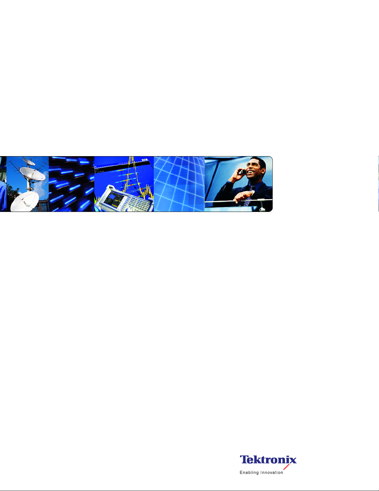
Figure 1-1: The swept spectrum analyzer steps across a series of frequency

segments, often missing important transient events that occur outside the current sweep band highlighted in yellow.

Analog and digital modulation analysis

Characterizing time-variant modulation schemes

Troubleshooting complex wireless standards using

domain correlation

Performing modulation quality diagnostics

Each measurement involves RF signals that change over time, often

unpredictably. To effectively characterize these signals, engineers

need a tool that can trigger on known or unpredictable events,

capture the signals seamlessly and store them in memory, and

analyze the behavior of frequency, amplitude, and modulation

parameters over time.

A Brief Survey of Instrument Architectures

The Real-Time Spectrum Analyzer (RTSA) is an innovative measure-

ment tool designed by Tektronix to address the emerging RF meas-

urement challenges described above. To learn how the RTSA works

and understand the value of the measurements it provides, it is

helpful to first examine two other types of traditional RF signal

analyzers: the swept spectrum analyzer (SA) and the vector signal

analyzer (VSA).

The Swept Spectrum Analyzer: Traditional Frequency Domain Analysis

The swept-tuned, superheterodyne spectrum analyzer is the tradi-

tional architecture that first enabled engineers to make frequency

domain measurements several decades ago. Originally built with

purely analog components, the swept SA has since evolved along

with the applications that it serves. Current generation swept SAs

includes digital elements such as ADCs, DSPs, and microproces-

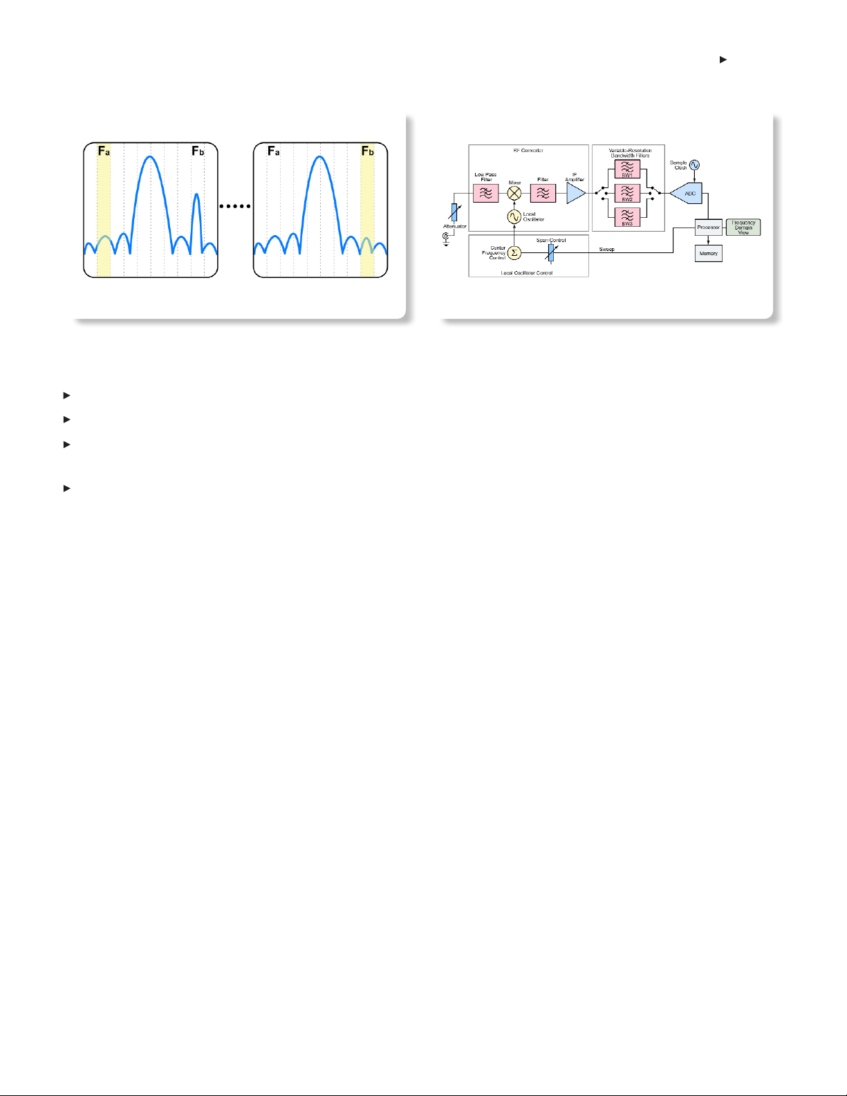
Figure 1-2: Typical swept spectrum analyzer architecture.

sors. However, the basic swept approach remains largely the same

and is best suited for observing controlled, static signals.

The swept SA makes power vs. frequency measurements by

downconverting the signal of interest and sweeping it through the

passband of a resolution bandwidth (RBW) filter. The RBW filter is

followed by a detector that calculates the amplitude at each fre-

quency point in the selected span. While this method can provide

high dynamic range, its disadvantage is that it can only calculate

the amplitude data for one frequency point at a time. Sweeping the

analyzer over a span of frequencies takes time – on the order of

seconds in some cases. This approach is based on the assumption

that the analyzer can complete several sweeps without there being

significant changes to the signal being measured. Consequently, a

relatively stable, unchanging input signal is required.

If there is a rapid change in the signal, it is statistically probable

that the change will be missed. As shown in Figure 1-1, the sweep

is looking at frequency segment Fa while a momentary spectral

event occurs at Fb(diagram on left). By the time the sweep arrives

at segment Fb, the event has vanished and does not get detected

(diagram on right). The SA does not provide a way to trigger on this

transient signal, nor can it store a comprehensive record of signal

behavior over time.

Figure 1-2 depicts a typical modern swept SA architecture. It

supplements the wide analog resolution bandwidth (RBW) filters

inherited from its predecessors with digital techniques to replace

the narrower filters. Filtering, mixing, and amplification prior to the

ADC are analog processes for bandwidths in the range of BW1,

BW2, or BW3. When filters narrower than “BW3” are needed, they

are applied by digital signal processing (DSP) in the steps following

the analog-to-digital conversion.

www.tektronix.com/rsa

Fundamentals of Real-Time Spectrum Analysis

Primer

The job of the ADC and the DSP is rather demanding. Non-linearity

and noise in the ADC are a challenge, although some types of errors

that can occur in purely analog spectrum analyzers are eliminated.

Vector Signal Analyzers: Digital Modulation Analysis

Traditional swept spectrum analysis enables scalar measurements

that provide information only about the magnitude of the input signal.

Analyzing signals carrying digital modulation requires vector measure-

ments that provide both magnitude and phase information. The vector

signal analyzer is a tool specifically designed for digital modulation

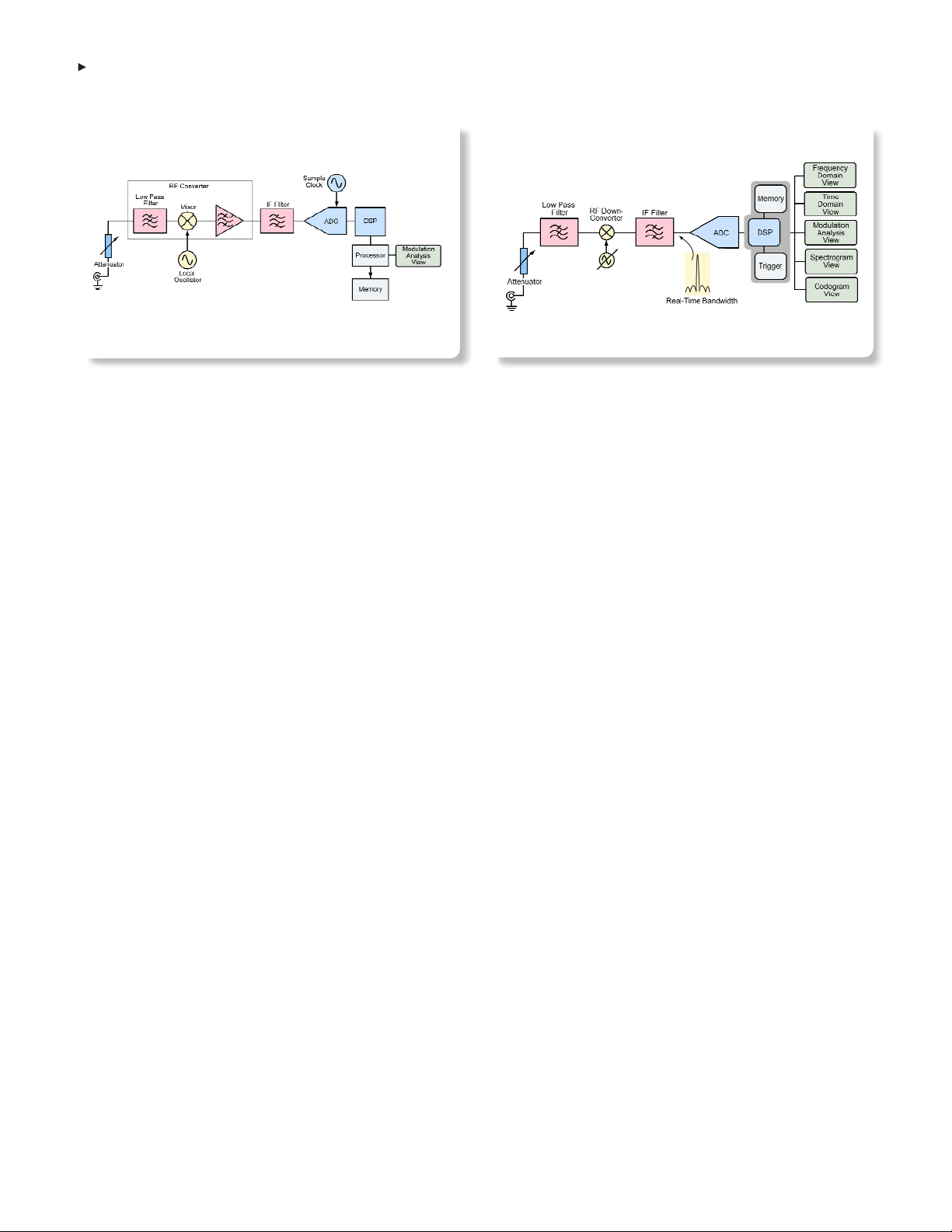
analysis. A simplified VSA block diagram is shown in Figure 1-3.

The VSA is optimized for modulation measurements. Like the

Real-Time Spectrum Analyzer described in the next section, a VSA

digitizes all of the RF energy within the passband of the instrument

in order to extract the magnitude and phase information required

to measure digital modulation. However, most (but not all) VSAs are

designed to take snapshots of the input signal at arbitrary points in

time, which makes it difficult or impossible to store a long record

of successive acquisitions for a cumulative history of how a signal

behaves over time. Like a swept SA, the triggering capabilities are

typically limited to an IF level trigger and an external trigger.

Within the VSA, an ADC digitizes the wideband IF signal, and the

down-conversion, filtering, and detection are performed numerically.

Transformation from time domain to frequency domain is done using

FFT algorithms. The linearity and dynamic range of the ADC are crit-

ical to the instrument’s performance. Equally important, there must

be sufficient DSP processing power to enable fast measurements.

The VSA measures modulation parameters such as Error Vector

Magnitude (EVM) and provides other displays such as the

constellation diagram. A standalone VSA is often used to supplement

the capabilities of a traditional swept SA. In addition, many modern

instruments have architectures that can perform both swept SA and

VSA functions, providing non-correlated frequency and modulation

domain measurements in one box.

Real-Time Spectrum Analyzers: Trigger, Capture, Analyze

The Real-Time Spectrum Analyzer is designed to address the

measurement challenges associated with transient and dynamic

RF signals as described in the previous section. The fundamental

concept of real-time spectrum analysis is the ability to trigger on

an RF signal, seamlessly capture it into memory, and analyze it in

multiple domains. This makes it possible to reliably detect and

characterize RF signals that change over time.

Figure 1-4 shows a simplified block diagram of the RTSA architec-

ture. (A more detailed diagram and circuit description appears in

Chapter 2). The RF front-end can be tuned across the entire frequen-

cy range of the instrument, and it down-converts the input signal to

a fixed IF that is related to the maximum real-time bandwidth of the

RTSA. The signal is then filtered, digitized by the ADC, and passed to

the DSP engine that manages the instrument’s triggering, memory,

and analysis functions. While elements of this block diagram and

acquisition process are similar to those of the VSA architecture, the

RTSA is optimized to deliver real-time triggering, seamless signal

capture, and time-correlated multi-domain analysis. In addition,

advancements in ADC technology enable a conversion with high

dynamic range and low noise, allowing the RTSA to equal or surpass

the basic RF performance of many swept spectrum analyzers.

www.tektronix.com/rsa

Figure 1-4: Typical real-time spectrum analyzer architecture.

Figure 1-3: Typical vector signal analyzer architecture.

Fundamentals of Real-Time Spectrum Analysis

Primer

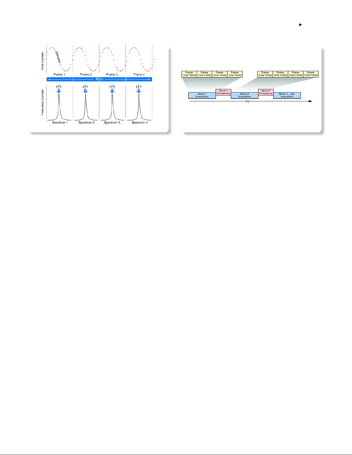
Figure 1-5: Samples, frames, and blocks: the memory hierarchy of the RSA.

For measurement spans less than or equal to the real-time band-

width, the RTSA architecture provides the ability to seamlessly

capture the input signal with no gaps in time by digitizing the RF

signal and storing the time-contiguous samples in memory. This has

several advantages over the acquisition process of a swept spectrum

analyzer, which builds up a frequency domain image by serially

sweeping across the frequency span. The remainder of this

document discusses these advantages in detail.

Key Concepts of Real-Time Spectrum Analysis

Samples, Frames, and Blocks

The measurements performed by the RTSA are implemented using

digital signal processing (DSP) techniques. To understand how an RF

signal can be analyzed in the time, frequency, and modulation

domains, it is first necessary to examine how the instrument

acquires and stores the signal. After it is digitized by the ADC, the

signal is represented by time domain data, from which all frequency

and modulation parameters can be calculated using DSP. These

concepts are discussed in detail in Chapter 2.

Three terms—samples, frames, and blocks—describe the hierarchy

of data stored when an RTSA seamlessly captures a signal using

real-time acquisition. Figure 1-5 illustrates the sample-frame-block

structure.

The lowest level of the hierarchy of data is the sample, which

represents a discrete time-domain data point. This construct is

familiar from other applications

Figure 1-6: Real-time spectrum analyzer block acquisition and processing.

of digital sampling, such as a real-time oscilloscopes and PC-based

digitizers. The effective sample rate which determines the time

interval between adjacent samples depends on the selected span. In

the RTSA, each sample is stored in memory as an I/Q pair contain-

ing magnitude and phase information.

The next step up is the frame.A frame consists of an integer number

of contiguous samples and is the basic unit to which the Fast Fourier

Transform (FFT) can be applied to convert time domain data into the

frequency domain. In this process, each frame yields one frequency

domain spectrum.

The highest level in the acquisition hierarchy is the block,which

is made up of many adjacent frames that are captured seamlessly

in time. The block length (also referred to as acquisition length) is

the total amount of time that is represented by one continuous

acquisition. Within a block, the input signal is represented with no

gaps in time.

In the real-time measurement modes of the RTSA, each block is

seamlessly acquired and stored into memory. It is then post-

processed using DSP techniques to analyze the frequency, time,

and modulation behavior of the signal. In standard SA modes, the

RTSA can emulate a swept SA by stepping the RF front end across

frequency spans that exceed the maximum real-time bandwidth.

Additional information can be found in Chapter 4.

Figure 1-6 shows block acquisition mode, which enables real-time

seamless capture. Each acquisition is seamless in time for all the

frames within a block, though not between blocks. After the signal

www.tektronix.com/rsa

Fundamentals of Real-Time Spectrum Analysis

Primer

processing of one acquisition block is complete, the acquisition of

the next block will begin. Once the block is stored in memory any

real-time measurements can be applied. For example, a signal

captured in real-time SA mode can then be analyzed in demod

mode and time mode.

The number of frames acquired within the block can be determined

by dividing the acquisition length by the frame length. The acquisi-

tion length entered by the user is rounded so the block contains an

integer number of frames. The maximum acquisition length ranges

from seconds to days and depends on the selected measurement

span and the memory depth of the instrument. Examples for specific

RTSAs are given in Chapter 4.

Real-Time Triggering

Useful triggering has long been a missing ingredient in most

spectrum analysis tools. The RTSA is the first mainstream spectrum

analyzer to offer real-time frequency domain triggering and other

intuitive trigger modes in addition to simple IF level and external

triggers. There are many reasons that the traditional swept

architecture is not well suited for real-time triggering, most signifi-

cantly that in a swept SA a trigger event is used to begin a sweep.

The RTSA, on the other hand, uses a trigger event as a reference

point in time for the seamless acquisition of the signal. This enables

several other useful features, such as the ability to store both pre-

trigger and post-trigger information. An in-depth discussion of the

real-time triggers of the RTSA can be found in Chapter 2.

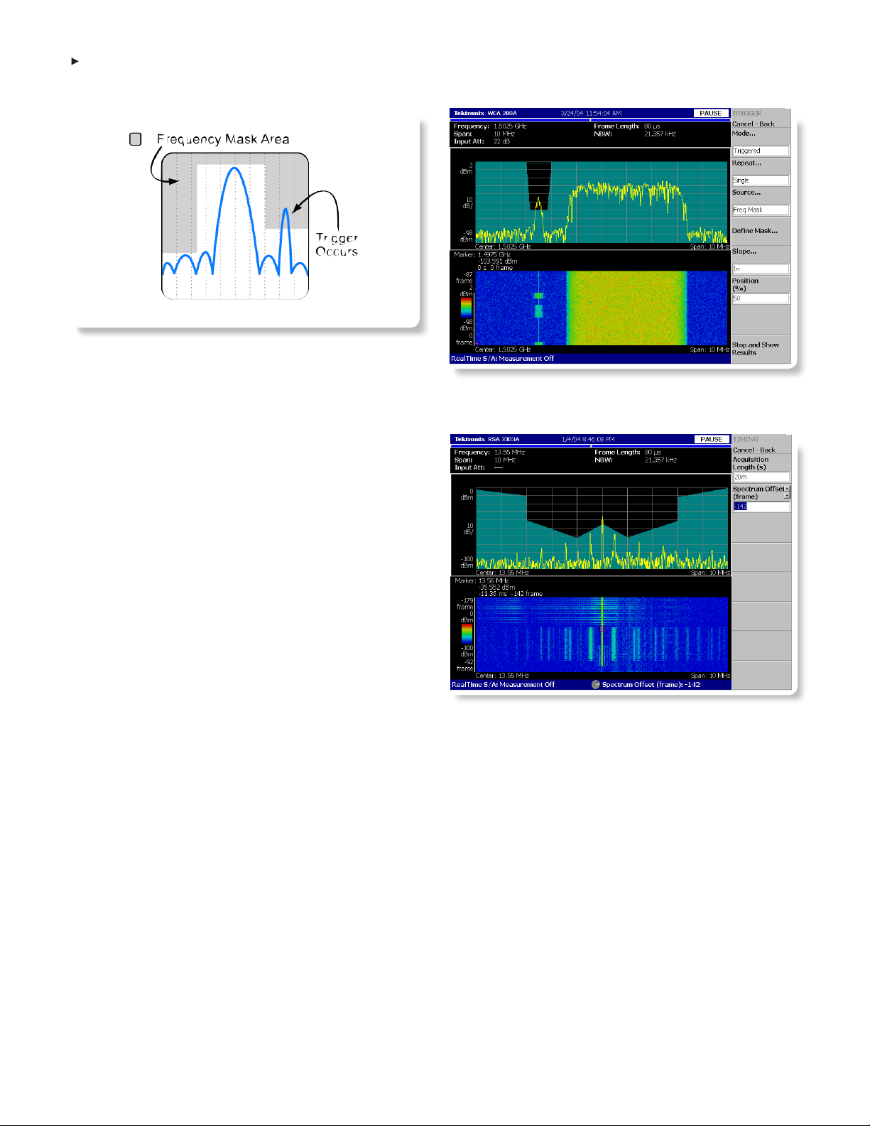
Another significant capability of the RTSA is the real-time frequency

mask trigger, which allows the user to trigger an acquisition based

on specific events in the frequency domain. As illustrated in

Figure 1-7, a mask is drawn to define the set of conditions within

the analyzer’s real-time bandwidth will generate the trigger event.

The flexible frequency mask trigger is a powerful tool for reliably

detecting and analyzing dynamic RF signals. It can be also used to

make measurements that are impossible with traditional spectrum

analyzers, such as capturing low-level transient events that occur in

the presence of more powerful RF signals (as shown in Figure 1-8)

and detecting intermittent signals at specific frequencies within a

crowded frequency spectrum (as shown in Figure 1-9).

www.tektronix.com/rsa

Figure 1-8: Using the frequency mask to trigger on a low level burst in the

presence of a large signal.

Figure 1-7: Real-time frequency domain triggering using a frequency mask.

Figure 1-9: Using the frequency mask to trigger on a specific signal in a

crowded spectral environment.

Fundamentals of Real-Time Spectrum Analysis

Primer

Figure 1-10: Spectrogram display.

Seamless Capture and Spectrogram

Once the real-time trigger conditions have been defined and the

instrument is armed to begin an acquisition, the RTSA continuously

examines the input signal to watch for the specified trigger event.

While waiting for this event to occur, the signal is constantly

digitized and the time domain data is cycled through a first-in,

first-out capture buffer that discards the oldest data as new data

is accumulated. This enables the analyzer to save pre-trigger and

post-trigger data into memory when it detects the trigger event.

As described in the sections above, this process enables a seam-

less acquisition of the specified block, within which a signal is

represented by contiguous time domain samples. Once this data has

been stored in memory, it is available to process and analyze using

different displays such as power vs. frequency, spectrogram, and

multi-domain views. The sample data remains available in random

access memory until it is overwritten by a subsequent acquisition,

and it can also be saved to the internal hard drive of the RTSA.

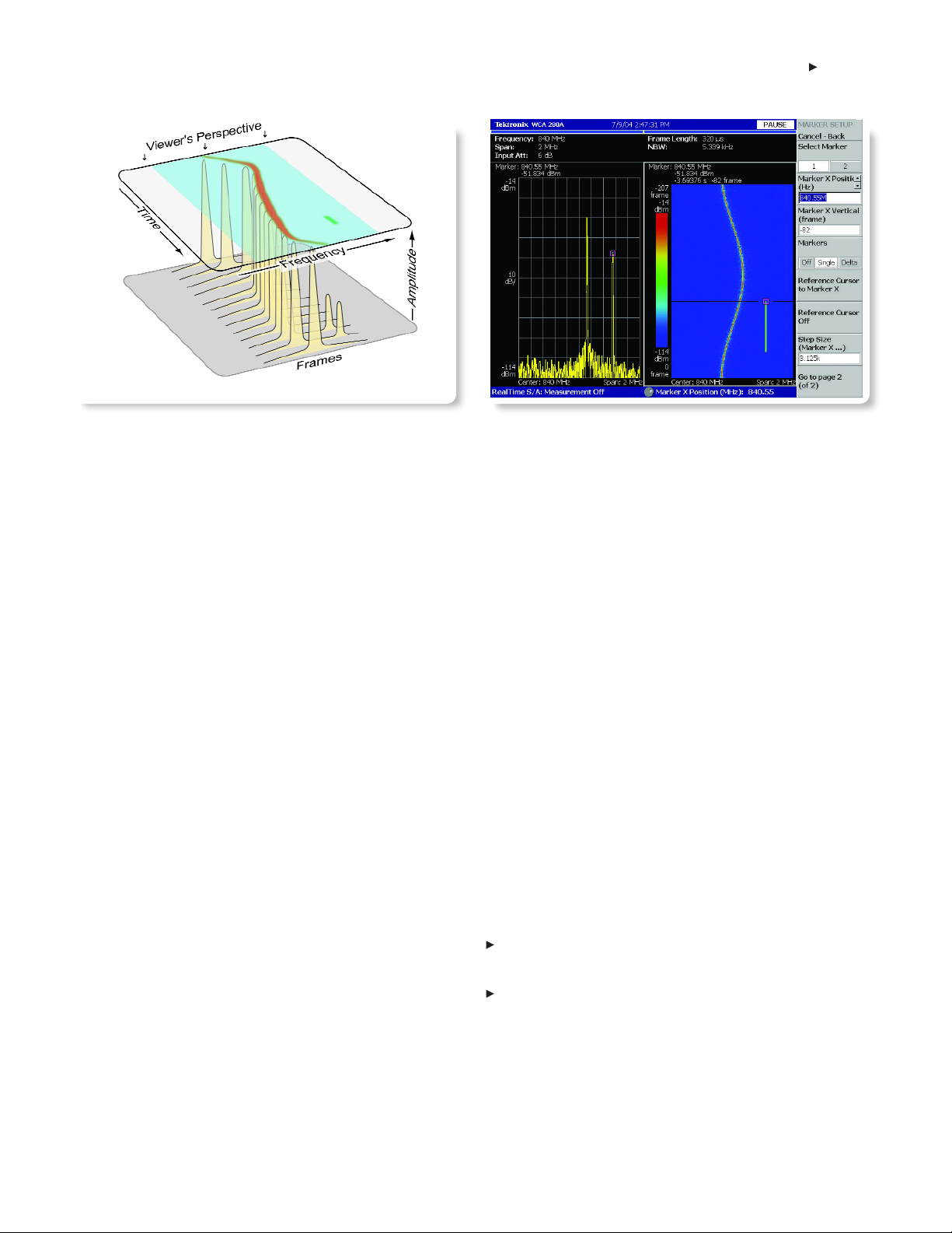
The spectrogram is an important measurement that provides an

intuitive display of how frequency and amplitude behavior change

over time. The horizontal axis represents the same range of fre-

quencies that a traditional spectrum analyzer shows on the power

vs. frequency display. In the spectrogram, though the vertical axis

represents time, and amplitude is represented by the color of the

trace. Each “slice” of the spectrogram corresponds to a single fre-

quency spectrum calculated from one frame of time domain data.

Figure 1-10 shows a conceptual illustration of the spectrogram of a

dynamic signal.

Figure 1-11: Time-correlated views: power vs. frequency display (left) and

spectrogram display (right).

Figure 1-11 shows a screen shot displaying the power vs. frequency

and spectrogram displays for the signal illustrated in Figure 1-10.

On the spectrogram, the oldest frame is shown at the top of the

display and the most recent frame is shown at the bottom of the

display. This measurement shows an RF signal whose frequency is

changing over time, and it also reveals a low level transient signal

that appears and disappears near the end of the time block. Since

the data is stored in memory, a marker can be used to scroll “back

in time” through the spectrogram. In Figure 1-11, a maker has been

placed on the transient event on the spectrogram display, which

causes the spectrum corresponding to that particular point in time

to be shown on the power vs. frequency display.

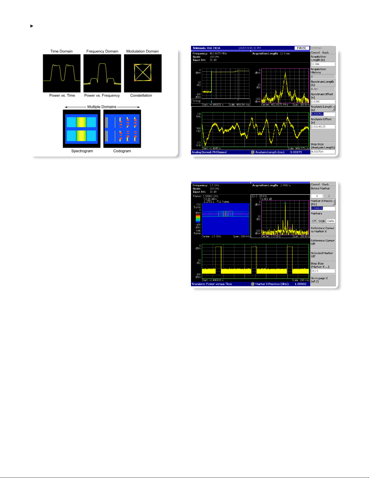
Time-Correlated Multi-Domain Analysis

Once a signal has been acquired and stored in memory, it can be

analyzed using the wide variety of time-correlated views available in

the RTSA, as illustrated in Figure 1-12 (next page).

This is especially useful for device troubleshooting and signal

characterization applications. All of these measurements are based

on the same underlying set of time domain sample data, which

underscores two significant architectural advantages:

Comprehensive signal analysis in the frequency, time, and

modulation domains based on a single acquisition.

Domain correlation to understand how specific events in the

frequency, time, and modulation domains are related based on

a common time reference.

www.tektronix.com/rsa

Fundamentals of Real-Time Spectrum Analysis

Primer

In real-time spectrum analysis mode, the RTSA provides two time-

correlated views of the captured signal: the power vs. frequency

display and the spectrogram display. These two views can be seen

in Figure 1-11.

In the other real-time measurement modes for time domain analysis

and modulation domain analysis, the RTSA shows multiple views of

the captured signal as illustrated in Figures 1-13 and 1-14. The

window in the upper left is called the overview, and it can display

either power vs. time or the spectrogram. The overview shows all of

the data that was acquired in the block, and it serves as the index

for the other analysis windows.

The window in the upper right (outlined in purple) is called the sub-

view, and it shows the same power vs. frequency display that is

available in Real-Time Spectrum Analyzer mode. Just like the dis-

play in Figure 1-11, this is the spectrum of one frame of data, and

it is possible to scroll through the entire time record to see the

spectrum at any point in time. This is done by adjusting the spec-

trum offset, which is found in the Timing menu of the RTSA. Also

note that there is a purple bar in the overview window that indicates

position in time that corresponds to the frequency domain display in

the purple subview window.

The window in the bottom half of the screen (outlined in green) is

called the analysis window, or mainview, and it displays the results

of the selected time or modulation analysis measurement.

Figure 1-13 shows an example of frequency modulation analysis,

and Figure 1-14 shows an example of transient power vs. time

analysis. Like the subview window, the green analysis window can

be positioned anywhere within the time record shown in the

overview window, which has corresponding green bars to indicate

its position. In addition, the width of the analysis window can be

flexibly adjusted to lengths less than or greater than one frame.

Time-correlated multi-domain analysis provides tremendous

flexibility to zoom in and thoroughly characterize different parts of

an acquired RF signal using a wide variety of analysis tools. An

introduction to these measurements can be found in Chapter 3.

www.tektronix.com/rsa

Figure 1-14: Multi-domain view showing spectrogram, power vs. frequency,

and power vs. time.

Figure 1-13: Multi-domain view showing power vs. time, power vs.

frequency, and FM demodulation.

Figure 1-12: Illustrations of several time-correlated measurements available

on RTSA’s.

www.tektronix.com/rsa

Fundamentals of Real-Time Spectrum Analysis

Primer

www.tektronix.com/rsa

Chapter 2: How a Real-Time Spectrum Analyzer Works

Modern Real-Time Spectrum Analyzers can acquire a passband, or

span, anywhere within the input frequency range of the analyzer. At

the heart of this capability is an RF down-converter followed by a

wideband intermediate frequency (IF) section. An ADC digitizes the

IF signal and the system carries out all further steps digitally. An

FFT algorithm implements the transformation from time domain to

frequency domain, where subsequent analysis produces displays

such as spectrograms, codograms, and more.

Several key characteristics distinguish a successful real-time

architecture:

An ADC system capable of digitizing the entire real-time BW with

sufficient fidelity to support the desired measurements.

An integrated signal analysis system that provides multiple

analysis views of the signal under test, all correlated in time.

Sufficient capture memory and DSP power to enable continuous

real-time acquisition over the desired time measurement period.

DSP power to enable real-time triggering in the frequency

domain.

This chapter contains several architectural diagrams of the main

acquisition and analysis blocks of the Tektronix Real-Time Spectrum

Analyzer (RSA). Some ancillary functions (minor triggering-related

blocks, display and keyboard controllers, etc.) have been omitted to

clarify the discussion.

Digital Signal Processing in Real-Time Spectrum Analyzers

Tektronix’ RSAs use a combination of analog and digital signal

processing to convert RF signals into calibrated, time-correlated

multi-domain measurements. This section deals with the digital

portion of the RSA signal processing flow.

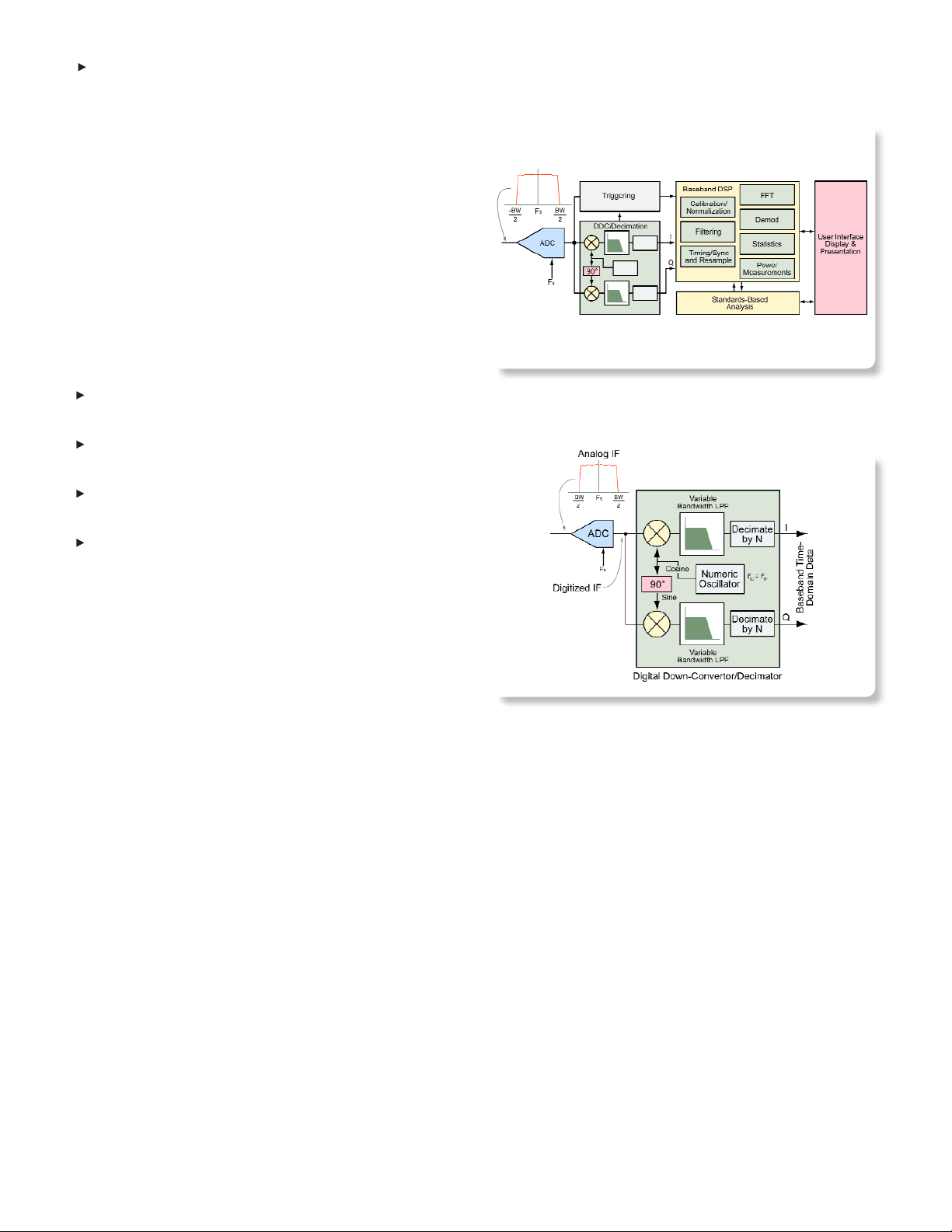
Figure 2-1 illustrates the major digital signal processing blocks

used in the Tektronix RSA Series. An analog IF signal is bandpass

filtered and digitized. A digital down-conversion and decimation

process converts the A/D samples into streams of in-phase (I) and

quadrature (Q) base band signals. A triggering block detects signal

conditions to control acquisition and timing. The baseband I and Q

signals as well as triggering information are used by a baseband

DSP system to perform spectrum analysis by means of FFT,

modulation analysis, power measurements, timing measurements

as well as statistical analyses.

IF Digitizer

Tektronix RSAs typically digitize a band of frequencies centered

around an intermediate frequency (IF). This band or span of fre-

quencies is the widest frequency for which real-time analysis can

be performed. Digitizing at a high IF rather than at DC or baseband

has several signal processing advantages (spurious performance,

DC rejection, dynamic range, etc.) but can require excessive compu-

tation to filter and analyze if processed directly. Tektronix RSAs

employ a digital down-converter (DDC), Figure 2-2 and a decimator

to convert a digitized IF into I and Q baseband signals at an effec-

tive sampling rate just high enough for the selected span.

Figure 2-1: Real-time spectrum analyzer digital signal processing

block diagram.

Figure 2-2: Digital down-converter block diagram.

Fundamentals of Real-Time Spectrum Analysis

Primer

Span Decimation (n) Effective Time

Sample Rate Resolution

15 MHz 2 25.6 MS/s 39.0625 ns

10 MHz 4 12.8 MS/s 78.1250 ns

1 MHz 40 1.28 MS/s 781.250 ns

100 KHz 400 128 KS/s 7.81250 s

10 KHz 4000 12.8 KS/s 78.1250 s

1 KHz 40000 1.28 KS/s 781.250 s

100 Hz 400000 128 S/s 7.81250 ms

Figure 2-3: Information in the passband is maintained in I and Q, even at

half the sample rate.

Digital Down Converter

The IF signal is digitized with sample rate FS. The digitized IF is then

sent to a DDC. A numeric oscillator in the DDC generates a sine and

a cosine at the center frequency of the band of interest. The sine

and cosine are numerically multiplied with the digitized IF, generating

streams of I and Q baseband samples that contain all of the informa-

tion present in the original IF. The I and Q streams then pass through

variable bandwidth low-pass filters. The cutoff frequency of the low-

pass filters is varied according to the selected span.

I and Q Baseband Signals

Figure 2-3 illustrates the process of taking a frequency band and converting it to baseband using quadrature down-conversion. The original IF signal is contained in the space between three halves of the sampling frequency and the sampling frequency. Sampling produces an image of this signal between zero and one-half the sampling frequency. The signal is then multiplied with coherent sine and cosine signals at the center of the passband of interest, generating I and Q baseband signals. The baseband signals are real-valued and symmetric about the origin. The same information is contained in the positive and negative frequencies. All of the modulation contained in the original passband is also contained in these two signals. The minimum required sampling frequency for each is now half of the original. It is then possible to decimate by two.

Table 2-1: Selected span, decimation and effective sample rates.

(Tektronix RSA3300A Series and WCA200A Series)

Decimation

The Nyquist theorem states that for baseband signals one need only sample at a rate equal to twice the highest frequency of interest. Time and frequency are reciprocal quantities. To study low frequencies it is necessary to observe a long record of time. Decimation is used to balance span, processing time, record length and memory usage.

The Tektronix RSA3300A Series, for example, uses a 51.2 MS/s

sampling rate at the A/D converter to digitize a 15 MHz bandwidth,

or span. The I and Q records that result after DDC, filtering and

decimation for this 15 MHz span are at an effective sampling rate

of half the original, that is, 25.6 MS/s. The total number of samples

is unchanged: we are left with two sets of samples, each at an

effective rate of 25.6 MS/s instead of a single set at 51.2 MS/s.

Further decimation is made for narrower spans, resulting in longer

time records for an equivalent number of samples. The disadvan-

tage of the lower effective sampling rate is a reduced time resolu-

tion. The advantages of the lower effective sampling rate are fewer

computations and less memory usage for a given time record, as

shown in Table 2-1.

Time and Frequency Domain Effects of Sampling Rate

Using decimation to reduce the effective sampling rate has several consequences for important time and frequency domain measurement parameters. An example contrasting a wide span and a narrow span is shown in Figures 2-4 and 2-5. A more through discussion and additional examples can be found in the FAQ in Chapter 4.

www.tektronix.com/rsa

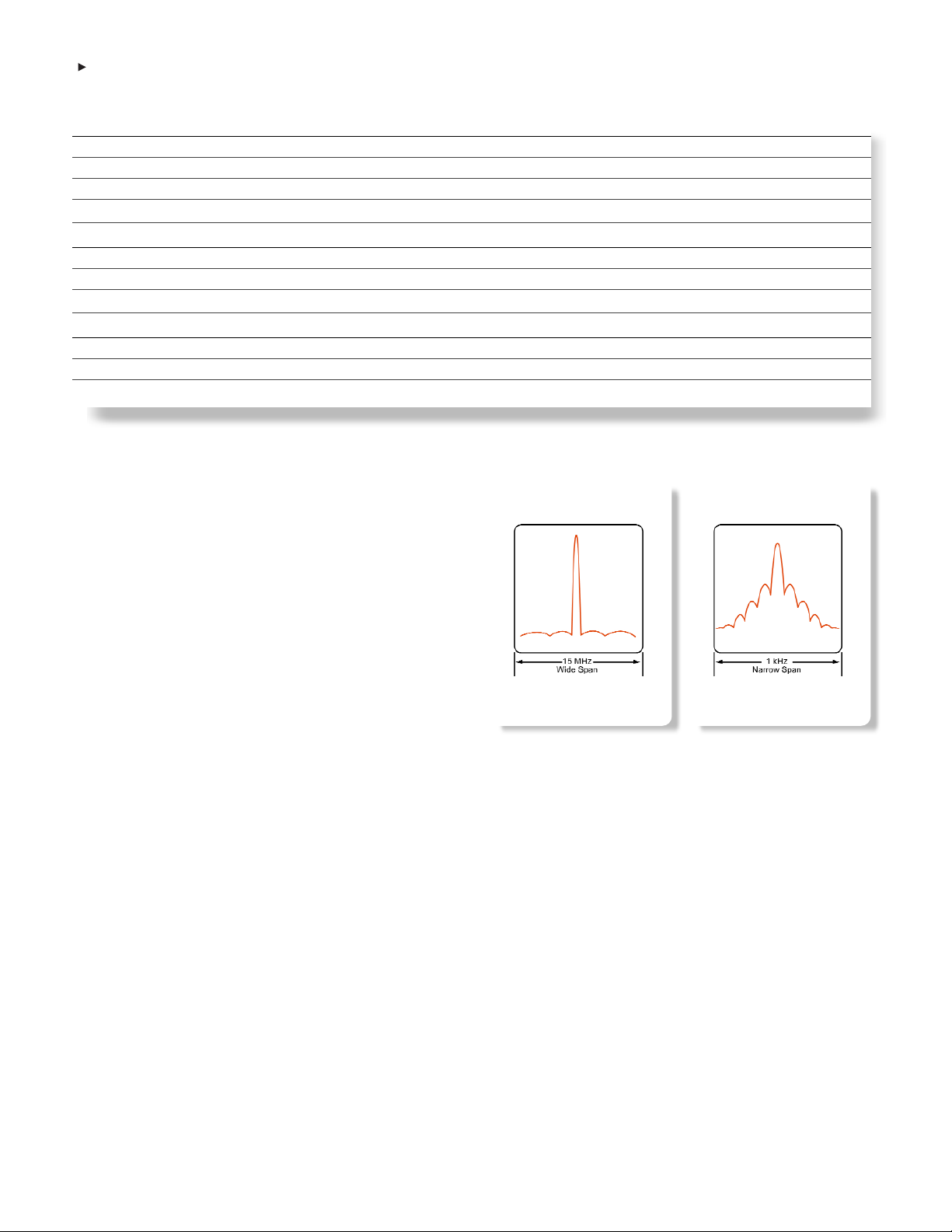
A wide capture bandwidth displays a broad span of frequencies with relatively low frequency domain resolution. Compared to narrower capture bandwidths, the sample rate is higher, and the resolution bandwidth is wider. In the time domain, frame length is shorter, and time resolution is finer. Record length is the same in terms of the number of stored samples, but the amount of time represented by these samples is shorter. Figure 2-4 illustrates a wide bandwidth capture, and Table 2-2 provides a real-world example.

In contrast, a narrow capture bandwidth displays a small span of frequencies with higher frequency domain resolution. Compared to wide capture bandwidths, the sample rate is lower, while the resolution bandwidth is narrower. In the time domain, the frame length is longer, time resolution is coarser, and the available record length encompasses more time. Figure 2-5 illustrates a narrow bandwidth capture, and Table 2-2 provides a real-world example. Note the scale of the numbers such as frequency resolution — they are several orders of magnitude different from the wideband capture.

Real-Time Triggering

The Real-Time Spectrum Analyzer adds the power of the time domain to spectrum and modulation analysis. Triggering is critical to capturing time domain information. The RSA offers unique trigger functionality, providing power and frequency-mask triggers as well as the usual external and level-based triggers.

The most common trigger system is the one used in most oscilloscopes. In traditional analog oscilloscopes, the signal to be observed is fed to one input while the trigger is fed to another. The trigger event causes the start of a horizontal sweep while the amplitude of the signal is shown as a vertical displacement superimposed on a calibrated graticule. In its simplest form, analog triggering allows events that happen after the trigger to be observed, as shown in Figure 2-6(next page)

Fundamentals of Real-Time Spectrum Analysis

Primer

www.tektronix.com/rsa

Figure 2-4: Wide capture bandwidth

example.

Figure 2-5: Narrow capture

bandwidth example.

Instrument Settings Wide span Narrow span

Span 15 MHz 1 kHz

Sample Rate 51.2 MS / second 51.2 MS / second

Decimation 2 32000

Effective Sample Rate 25.6 MS / second 1.6 kS / second

Time Domain Effects

Time Domain Resolution (sample) 39.0 nanoseconds 625 microseconds

Spectrogram Time Resolution (frame length) 40.0 microseconds 640 milliseconds

Maximum Record Length (256 MB memory) 2.56 seconds 11.4 hours

Frequency Domain Effects

Frequency Resolution (FFT bin width) 25.0 kHz 1.56 Hz

NBW (noise bandwidth) 43.7 kHz 2.67 Hz

Equivalent Gaussian RBW 41.2 kHz 2.52 Hz

Table 2-2: Comparison of time and frequency domain effects of changing the span setting. (Tektronix RSA3300A Series and WCA200A Series)

Figure 2-6: Traditional oscilloscope triggering.

Fundamentals of Real-Time Spectrum Analysis

Primer

Figure 2-7: Triggering in digital acquisition systems.

Triggering in Systems with Digital Acquisition

The ability to represent and process signals digitally, coupled with

large memory capacity, allows the capture of events that happen

before the trigger as well as after it.

Digital acquisition systems of the type used in Tektronix RSAs use

an Analog-to-Digital Converter (ADC) to fill a deep memory with

time samples of the received signal. Conceptually, new samples

are continuously fed to the memory while the oldest samples fall off.

The example shown in Figure 2-7 shows a memory configured to

store N samples. The arrival of a trigger stops the acquisition, freez-

ing the contents of the memory. The addition of a variable delay in

the path of the trigger signal allows events that happen before a

trigger as well as those that come after it to be captured.

Consider a case in which there is no delay. The trigger event causes

the memory to freeze immediately after a sample concurrent with

the trigger is stored. The memory then contains the sample at the

time of the trigger as well as “N” samples that occurred before the

trigger. Only pre-trigger events are stored.

Consider now the case in which the delay is set to match exactly

the length of the memory. “N” samples are then allowed to come

into the memory after the trigger occurrence before the memory is

frozen. The memory then contains “N” samples of signal activity

after the trigger. Only post-trigger events are stored.

Both post and pre-trigger events can be captured if the delay is set

to a fraction of the memory length. If the delay is set to half of the

memory depth, half of the stored samples are those that preceded

the trigger and half the stored samples followed it. This concept is

similar to a trigger delay used in zero span mode of a conventional

swept SA. The RSA can capture much longer time records, however,

and this signal data can subsequently be analyzed in the frequency,

time, and modulation domains. This is a powerful tool for applica-

tions such as signal monitoring and device troubleshooting.

Trigger Modes and Features

The free-run mode acquires samples of the received IF signal

without the consideration of any trigger conditions. Spectrum,

modulation or other measurements are displayed as they are

acquired and processed.

The triggered mode requires a trigger source as well as the setting

of various parameters that define the conditions for triggering as

well as the instrument behavior in response to a trigger.

A selection of continuous or single trigger determines whether

acquisitions repeat each time a trigger occurs or are taken only

once each time a measurement is armed. The trigger position,

adjustable from 0 to 100%, selects which portion of an acquisition

block is pre-trigger. A selection of 10% captures pre-trigger data for

one tenth of the selected block and post-trigger data for nine

tenths. Trigger slope allows the selection of rising edges, falling

www.tektronix.com/rsa

edges or their combination for triggering. Rise and fall allows the

capture of complete bursts. Fall and rise allows the capture of gaps

in an otherwise continuous signal.

RSA Trigger Sources

Tektronix RSAs provide several methods of internal and external

triggering.

Table 2-3 summarizes the various real-time trigger

sources, their settings, and the time resolution that is associated

with each one.

External triggering allows an external TTL signal to control the

acquisition. This is typically a control signal such as a frequency

switching command from the system under test. This external signal

prompts the acquisition of an event in the system under test.

Internal triggering depends on the characteristics of the signal

being tested. The RSA has the ability to trigger on the level of the

digitized signal, on the power of the signal after filtering and

decimation, or on the occurrence of specific spectral components

using the frequency mask trigger. Each of the trigger sources and

modes offers specific advantages in terms of frequency selectivity,

time resolution and dynamic range. The functional elements that

support these features are shown in Figure 2-8 (next page).

Level triggering compares the digitized signal at the output of the

ADC with a user-selected setting. The full bandwidth of the digitized

signal is used, even when observing narrow spans that require

further filtering and decimation. Level triggering uses the full

digitization rate and can detect events with durations as brief as

one sample at the full sampling rate. The time resolution of the

downstream analyses, however, is limited to the decimated effective

sampling rate. The trigger level is set as a percentage of the ADC

clip level, that is, its maximum binary value (all “ones”). This is a

linear quantity not to be confused with the logarithmic display,

which is expressed in dB.

Power triggering calculates the power of the signal after filtering

and decimation. The power of each filtered pair of I/Q samples

2+Q2

) is compared with a user-selected power setting. The setting

is in dB relative to full scale (dBfs) as shown on the logarithmic

screen. A setting of 0 dBfs places the trigger level at the top graticule

and will generate a trigger when the total power contained in the

span exceeds that trigger level. A setting of -10 dBfs will trigger

when the total power in the span reaches a level 10 dB below the

top graticule. Note that the total power in the span generates a

trigger. Two CW signals each at a level of -3 dBm, for example,

have an aggregate power of 0 dBm.

Frequency mask triggering compares the spectrum shape to a

user-defined mask. This powerful technique allows changes in a

spectrum shape to trigger an acquisition. Frequency mask triggers

can reliably detect signals far below full-scale even in the presence

of other signals at much higher levels. This ability to trigger on

weak signals in the presence of strong ones is critical for detecting

intermittent signals, the presence of inter-modulation products,

Fundamentals of Real-Time Spectrum Analysis

Primer

www.tektronix.com/rsa

Trigger Source Trigger Signal Setting Units Time Resolution Notes

External External trigger TTL level Time domain External control

connector signal points (based on signals

effective sampling rate)

Level Level comparator % A/D Full Scale Time domain Full IF bandwidth

at A/D output points (based on

effective sampling rate)

Power Power calculation dB Full Scale Time domain Bandwidth defined

at DDC/Decimator relative to the top points (based on) by the span setting output graticule effective sampling

rate

Frequency mask Point by point dB and Hz, based Frame length Flexible mask

comparison at the on the graphical (based on effective profile defined by output of a FFT mask drawn on sampling rate) user Processor screen

Table 2-3: Comparison of RSA trigger sources.

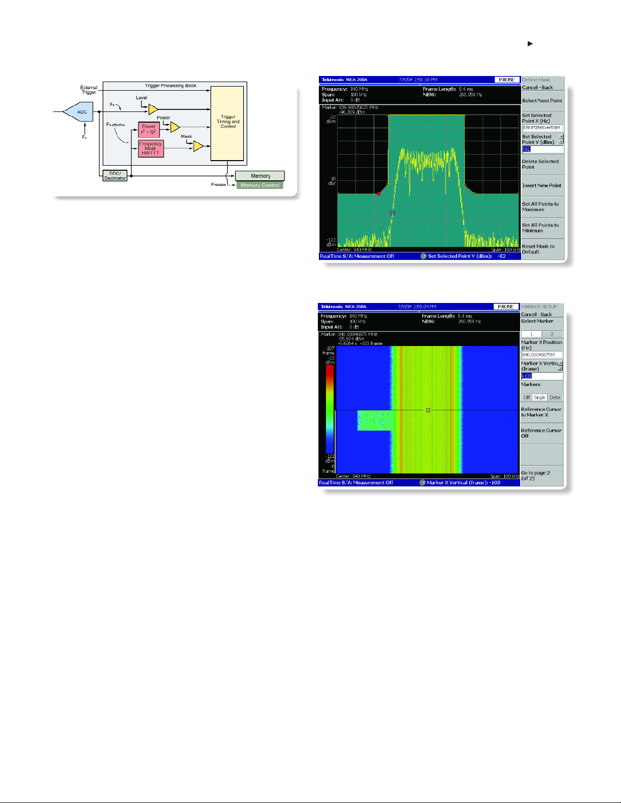
Fundamentals of Real-Time Spectrum Analysis

Figure 2-8: Real-time spectrum analyzer trigger processing.

transient spectrum containment violations and much more. A full

FFT is required to compare a signal to a mask, requiring a complete

frame. The time resolution for frequency mask trigger is roughly one

FFT frame, or 1024 samples at the effective sampling rate. Trigger

events are determined in the frequency domain using a dedicated

hardware FFT processor, as shown in the block diagram in

Figure 2-8.

Primer

Figure 2-9: Frequency mask definition.

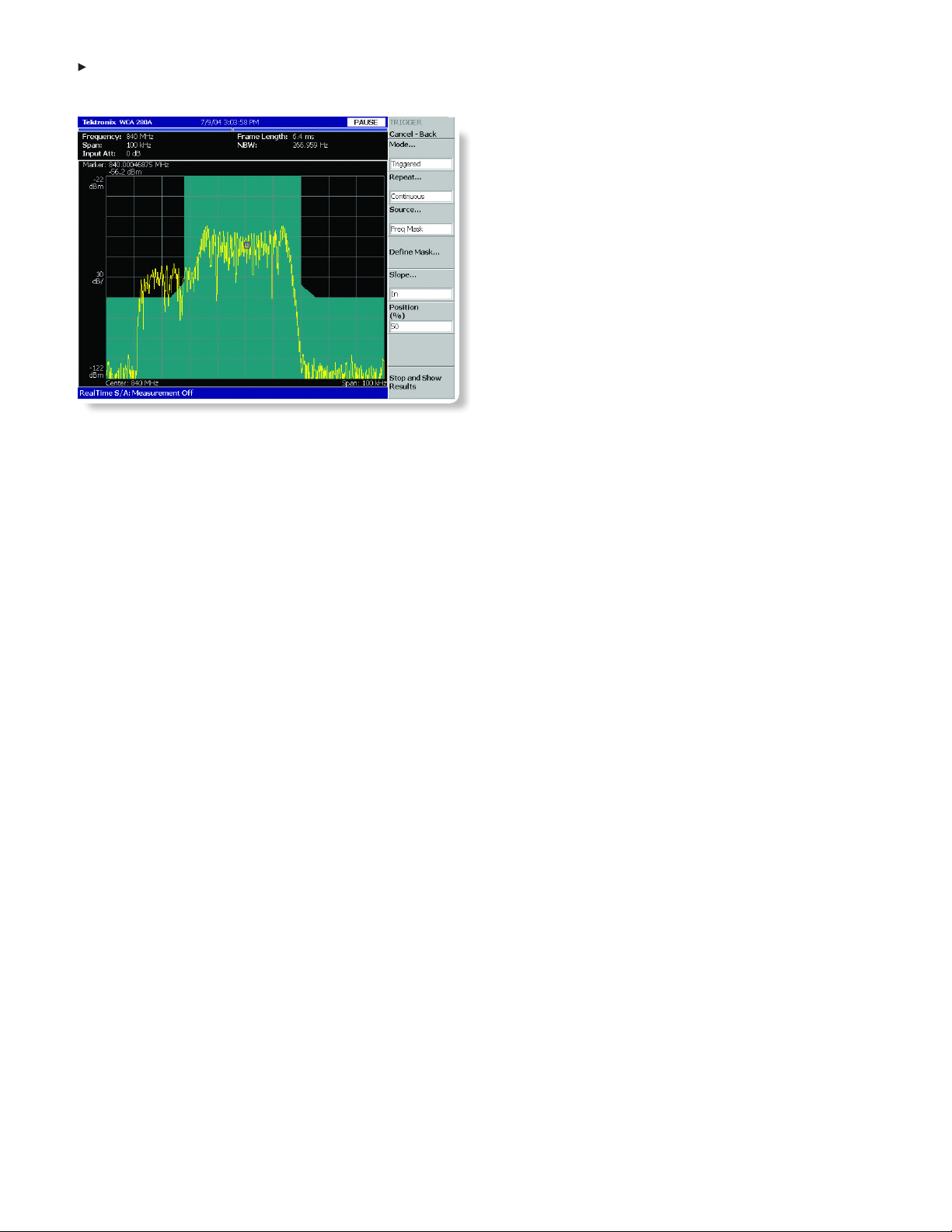
Constructing a Frequency Mask

Like other forms of mask testing, the frequency mask trigger (also

known as frequency domain trigger) starts with a definition of on

on-screen mask. This definition is done with a set of frequency

points and their amplitudes. The mask can be defined point-by-point

or graphically by drawing it with a mouse or other pointing device.

Triggers can be set to occur when a signal outside the mask

boundary “breaks in,” or when a signal inside the mask boundary

“breaks out.”

Figure 2-9 shows a frequency mask defined to allow the passage

of the normal spectrum of a signal but not momentary aberrations.

Figure 2-10 shows a spectrogram display for an acquisition that

was triggered when the signal momentarily exceeded the mask.

Figure 2-11 (next page) shows the spectrum for one the first frame

where the mask was exceeded. Note that pre-trigger and post-

trigger data were collected and are both shown in the spectrogram.

Figure 2-10: Spectrogram showing a transient signal adjacent to the carrier.

The cursor is set to the trigger point, so pre-trigger data is displayed above the cursor line, and post-trigger data is displayed below the cursor line. The narrow white line at the left of the blue area denotes post-trigger data.

www.tektronix.com/rsa

Timing and Triggers

The timing controls, when used in conjunction with triggers offer a

powerful combination for analyzing transient or other timing related

parameters.

The acquisition length specifies the length of time for which

samples will be stored in memory in response to a trigger. The

acquisition history determines how many previous acquisitions

will be kept after each new trigger. Tektronix RSAs show the entire

acquisition length in the time-domain overview window.

The spectrum length determines the length of time for which

spectrum displays are calculated. The spectrum offset determines

the delay or advance from the instant of the trigger event until the

beginning of the FFT frame that is displayed. Both spectrum length

and spectrum offset have a time resolution of one FFT frame (1024

samples at the effective sample rate). Tektronix RSAs indicate the

spectrum offset and spectrum length using a colored bar at the

bottom of the time domain overview window. The bar color is keyed

to the pertinent display.

The analysis length determines the length of time for which modu-

lation analysis and other time based measurements are made. The

analysis offset determines the delay or advance from the instant of

the trigger until the beginning of the analysis. Tektronix RSAs

indicate the analysis offset and length using a colored bar at the

bottom of the time domain overview window. The bar color is keyed

to the pertinent display.

The output trigger indicator allows the user to selectively enable a

TTL rear panel output at the instant of a trigger. This can be used to

synchronize RSA measurements with other instruments such as

oscilloscopes or logic analyzers.

Baseband DSP

Virtually all Real-Time Spectrum Analyzer measurements are

performed through Digital Signal Processing (DSP) of the I and Q

data streams generated by the DDC/Decimation block and stored

into acquisition memory. The following is a description of some of

the main functional blocks that are implemented with DSP.

Calibration/Normalization

Calibrations and normalizations compensate for the gain and

frequency response of the analog circuitry that precedes the A/D

converter. Calibrations are performed at the factory and stored in

memory as calibration tables. Corrections from the stored tables

are applied to measurements as they are computed. Calibrations

provide accuracy traceable to official standards bodies.

Normalizations are measurements that are performed internally to

correct for variations caused by temperature changes, aging and

unit-to-unit differences. Like calibrations, normalization constants

are stored in memory and applied as corrections to measurement

computations.

Filtering

Many measurements and calibration processes require filtering in

addition to the filters in the IF and DDC/decimator. Filtering is done

numerically on the I and Q samples stored in memory.

Timing, Synchronization and Re-sampling

Timing relationships among signals are critical to many modern

RF systems. Tektronix RSAs provide time-correlated analysis of

spectrum, modulation and power allowing the time relationships

between various RF characteristics to be measured and studied.

Clock synchronization and signal re-sampling are needed for

demodulation and pulse processing.

Fundamentals of Real-Time Spectrum Analysis

Primer

www.tektronix.com/rsa

Figure 2-11: One frame of the spectrogram showing the trigger event

where the transient signal breaks the boundary of the frequency mask.

Fundamentals of Real-Time Spectrum Analysis

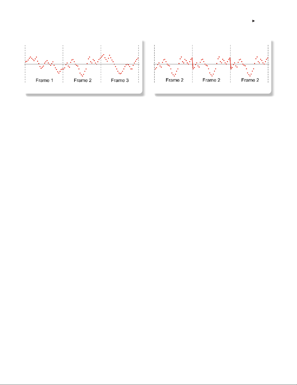
Primer

Figure 2-12: Three frames of a sampled time domain signal.

Fast Fourier Transform Analysis

The Fast Fourier Transform (FFT) is the heart of the real-time

spectrum analyzer. In the RSA, FFT algorithms are generally

employed to transform time-domain signals into frequency-domain

spectra. Conceptually, FFT processing can be considered as passing

a signal through a bank of parallel filters with equal frequency

resolution and bandwidth. The FFT output is generally complex–

valued. For spectrum analysis, the amplitude of the complex result

is usually of most interest.

The FFT process starts with properly decimated and filtered base-

band I and Q components, which form the complex representation

of the signal with I as its real part and Q as its imaginary part. In

FFT processing, a set of samples of the complex I and Q signals are

processed at the same time. This set of samples is called the FFT

frame. The FFT acts on a sampled time signal and produces a sam-

pled frequency function with the same length. The number of sam-

ples in the FFT, generally a power of 2, is also called the FFT size.

For example, 1024 point FFT can transform 1024 I and 1024 Q

samples into 1024 complex frequency-domain points.

FFT Properties

The amount of time represented by the set of samples upon which

the FFT is performed is called the frame length in the RSA. The

frame length is the product of the FFT size and the sample period.

Since the calculated spectrum is the frequency representation of the

signal over the duration of the frame length, temporal events can

not be resolved within the frame length from the corresponding

spectrum. Therefore, the frame length is the time resolution of the

FFT process.

The frequency domain points of FFT processing are often called FFT

bins. Therefore, the FFT size is equal to the number of bins in one

FFT frame. Those bins are equivalent to the individual filter output

Figure 2-13: Discontinuities caused by periodic extension of samples in a

single frame.

in the previous discussion of parallel filters. All bins are spaced

equally in frequency. Two spectral lines closer than the bin width

cannot be resolved. The FFT frequency resolution is therefore the

width of each frequency bin, which is equal to the sample frequency

divided by the FFT size. Given the same sample frequency, a larger

FFT size yields finer frequency resolution. For an RSA with a sample

rate of 25.6 MHz and an FFT size of 1024, the frequency resolution

is 25 kHz.

Frequency resolution can be improved by increasing the FFT size or

by reducing the sampling frequency. The RSA, as mentioned above,

uses a Digital Down Converter and Decimator to reduce the effective

sampling rate as the frequency span is narrowed, effectively trading

time resolution for frequency resolution while keeping the FFT size

and computational complexity to manageable levels. This approach

allows fine resolution on narrow spans without excessive computation

time on wide spans where coarser frequency resolution is sufficient.

The practical limit on FFT size is often display resolution, since an

FFT with resolution much higher than the number of display points

will not provide any additional information on the screen of the

instrument.

Windowing

There is an assumption inherent in the mathematics of Discrete

Fourier Transforms and FFT analysis that the data to be processed

is a single period of a periodically repeating signal. Figure 2-12

depicts a series of time domain samples. When FFT processing is

applied to Frame 2, for example, the periodic extension is made

to the signal. The discontinuities between successive frames will

generally occur as shown in Figure 2-13.

These artificial discontinuities generate spurious responses not

present in the original signal, which can make it impossible to

detect small signals in the presence of nearby large ones. This

effect is called spectral leakage.

www.tektronix.com/rsa

Tektronix RSAs apply a windowing technique to the FFT frame

before FFT processing is performed to reduce the effects of spectral

leakage. The window functions usually have a bell shape. There are

numerous window functions available. The popular Blackman-Harris

4B(BH4B) profile is shown in Figure 2-14.

The Blackman-Harris 4B windowing function shown in Figure 2-11 has

a value of zero for the first and last samples and a continuous curve

in between. Multiplying the FFT frame by the window function reduces

the discontinuities at the ends of the frame. In the case of the

Blackman-Harris window, we can eliminate discontinuities altogether.

The effect of windowing is to place a higher weight to the samples

in the center of the window than those away from the center,

bringing the value to zero at the ends. This can be thought of as

effectively reducing the time over which the FFT is calculated.

Time and frequency are reciprocal quantities. A smaller time sample

implies poorer (wider) frequency resolution. For Blackman-Harris 4B

windows, the effective frequency resolution is approximately twice

as wide as the value achieved without windowing.

Another implication of windowing is that the time-domain data mod-

ified by this window produces an FFT output spectrum that is most

sensitive to behavior in the center of the frame, and insensitive to

behavior at the beginning and end of the frame. Transient signals

appearing close to either end of the FFT frame are de-emphasized

and can be missed altogether. This problem can be resolved by use

of overlapping frames, a complex technique involving trade-offs

between computation time and time-domain flatness in order to

achieve the desired performance. This is briefly described below.

Post-FFT Signal Processing

Because the window function attenuates the signal at both ends of

the frame, it reduces the overall signal power, the amplitude of the

spectrum measured from the FFT with windowing must be scaled to

deliver a correct amplitude reading. For a pure sine wave signal, the

scaling factor is the DC gain of the window function.

Post processing is also used to calculate the spectrum amplitude by

summing the squared real part and the squared imaginary part at

each FFT bin. The spectrum amplitude is generally displayed in the

logarithmic scale so different frequencies with wide-ranging ampli-

tudes can be simultaneously displayed on the same screen.

Overlapping Frames

Some Real-Time Spectrum Analyzers can operate in real-time mode

with overlapping frames. When this happens, the previous frame is

being processed at the same time the new frame is being acquired.

Figure 2-15 shows how frames are acquired and processed.

One benefit of overlapping frames is an increased display update

rate, an effect that is most noticeable in narrow spans requiring

long acquisition times. Without overlapping frames, the display

screen cannot be updated until an entire new frame is acquired.

With overlapping frames, new frames are displayed before the

previous frame is finished.

Another benefit is a seamless frequency domain display in the spec-

trogram display. Since the windowing filter reduces the contribution

of the samples at each end of a frame to zero, spectral events

happening at the joint between two adjacent frames can be lost if

the frames do not overlap. However, having frames that overlap

ensures that all spectral events will be visible on the spectrogram

display regardless of windowing effects.

Fundamentals of Real-Time Spectrum Analysis

Primer

www.tektronix.com/rsa

Figure 2-14: Blackman-Harris 4B (BH4B) window profile.

Figure 2-15: Signal acquisition, processing, and display using

overlapping frames.

Fundamentals of Real-Time Spectrum Analysis

Primer

Figure 2-17: Typical digital communications system.Figure 2-16: Vector representation of magnitude and phase.

Modulation Analysis

Modulation is the means through which RF signals carry information.

Modulation analysis using the Tektronix RSA not only extracts the

data being transmitted but also measures the accuracy with which

signals are modulated. Moreover, it quantifies many of the errors and

impairments that degrade modulation quality.

Modern communications systems have dramatically increased the

number of modulation formats in use. The RSA is capable of analyzing

the most common formats and has an architecture that allows for the

analysis of new formats as they emerge.

Amplitude, Frequency and Phase Modulation

RF carriers can transport information in many ways based on varia-

tions in the amplitude or phase of the carrier. Frequency is the time

derivative of phase. Frequency Modulation (FM) is therefore the time

derivative of Phase Modulation (PM). Quadrature Phase Shift Keying

(QPSK) is a digital modulation format in which the symbol decision

points occur at multiple of 90 degrees of phase. Quadrature

Amplitude Modulation (AM) is a high-order modulation format in

which both amplitude and phase are varied simultaneously to pro-

vide multiple states. Even highly complex modulation formats such

as Orthoganal Frequency Division Multiplexing (OFDM) can be

decomposed into magnitude and phase components.

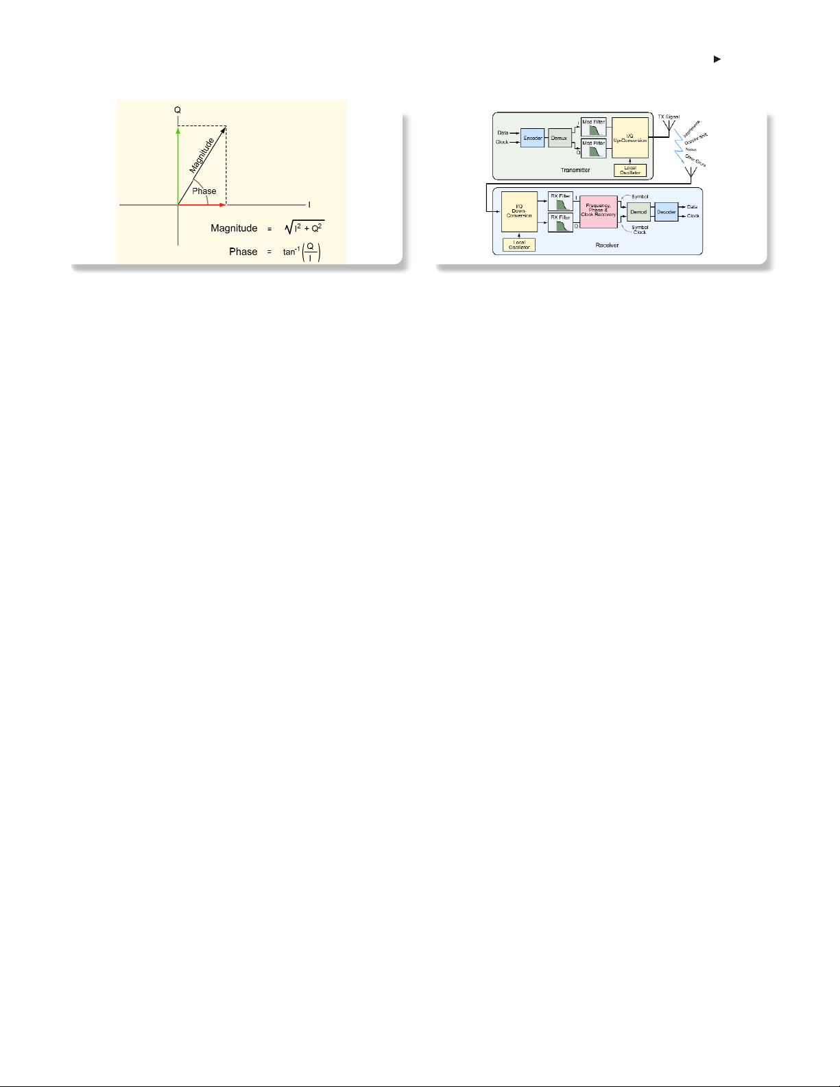
Magnitude and phase can be thought of as the length and the angle

of a vector in a polar coordinate system. The same point can be

expressed in Cartesian or rectangular coordinates (X,Y). The I/Q

format of the time samples stored in memory by the RSA are

mathematically equivalent to Cartesian coordinates with I representing

the horizontal or X component and Q the vertical or Y component.

Figure 2-16 illustrates the magnitude and phase of a vector along

with its I and Q components. AM demodulation consists of comput-

ing the instantaneous magnitude for each I/Q sample stored in

memory and plotting the result over time. PM demodulation consists

of computing the phase angle of the I and Q samples in memory

and plotting them over time after accounting for the discontinuities of the arctangent function at ±π/2. Once the phase trajectory or PM

is computed for a time record, FM can be calculated by taking the

time derivative.

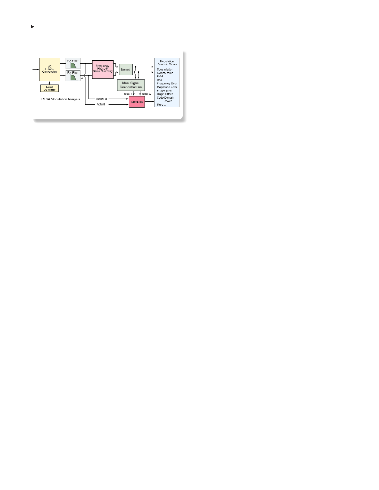
Digital Modulation

Figure 2-17 shows the signal processing in a typical digital commu-

nications system. The transmit process starts with the data to be

sent and a clock. The data and clock are passed through an

encoder that re-arranges the data, adds synchronization bits, and

does error recovery encoding and scrambling. The data is then split

into I and Q paths and filtered, changing it from bits to analog

waveforms which are then up-converted to the appropriate channel

and transmitted over the air. Once transmitted, the signal inevitably

suffers degradations from the environment before it is received.

The process of reception is the reverse of transmission with some

additional steps. The RF signal is down-converted to I and Q base-

band signals which are passed through RX filters often designed to

remove inter-symbol interference. The signal is then passed through

an algorithm that recovers the exact frequency, phase and data

clock. This is necessary to correct for multi-path delay and Doppler

shift in the path and for the fact that the RX and TX local oscillators

are not usually synchronized. Once frequency, phase and clock

are recovered, the signal is demodulated and decoded, errors are

corrected and bits are recovered.

www.tektronix.com/rsa

The varieties of digital modulation are numerous and include the

familiar FSK, BPSK, QPSK, GMSK, QAM, OFDM and others. Digital

modulation is often combined with channel assignments, filtering,

power control, error correction and communications protocols to

encompass a particular digital communication standard whose

purpose is to transmit error-free bits of information between radios

at opposite ends of a link. Much of the complexity incurred in a

digital communication format is necessary to compensate for the

errors and impairments that enter the system as the signal travels

over the air.

Figure 2-18 illustrates the signal processing steps required for a

digital modulation analysis. The basic process is the same as that

of a receiver except that recovered symbols are used to reconstruct

the mathematically ideal I and Q signals. These ideal signals are

compared with the actual or degraded I and Q signals to generate

the required modulation analysis views and measurements.

Power Measurements and Statistics

Tektronix RSAs can perform power measurements both in the

frequency domain and in the time domain. Time domain measure-

ments are made by integrating the power in the I and Q baseband

signals stored in memory over a specified time interval. Frequency

domain measurements are made by integrating the power in the

spectrum over a specified frequency interval. Channel filters,

required for many standards-based measurements, may be applied

to yield the resultant channel power. Calibration and normalization

parameters are also applied to maintain accuracy under all specified

conditions.

Communications standards often specify statistical measurements

for components and end-user devices. RSAs have measurement

routines to calculate statistics such as the Complementary

Cumulative Distribution Function (CCDF) of a signal which is often

used to characterize the peak-to-average power behavior of

complex modulated signals.

Fundamentals of Real-Time Spectrum Analysis

Primer

www.tektronix.com

Figure 2-18: RSA modulation analysis block diagram.

www.tektronix.com

Fundamentals of Real-Time Spectrum Analysis

Primer

www.tektronix.com/rsa

Chapter 3: Real-Time Spectrum Analyzer Measurements

This chapter describes the operational modes and measurements of

RSAs. Several pertinent details such as the sampling rate and the

number of FFT points are product dependent. Like the other meas-

urement examples in this document, the information in this section

applies specifically to the Tektronix RSA3300A Series and WCA200A

Series of Real-Time Spectrum Analyzers.

Frequency Domain Measurements

Real-Time SA

This is the mode described in the discussion of seamless capture

with spectrogram in Chapter 1. It provides real-time seamless

capture, real-time triggering, and the ability to analyze captured

time domain data using the power vs. frequency display and the

spectrogram display. This mode also provides several automated

measurements such as the carrier frequency measurement shown

in Figure 3-1.

As explained in Chapter 1, the spectrogram has three axes:

The horizontal axis represents frequency

The vertical axis represents time

The color represents amplitude

When combined with real-time triggering capabilities, as shown in

Figure 3-2, the spectrogram becomes an even more powerful meas-

urement tool for dynamic RF signals.

Here are a few key points to remember when using the spectrogram

display:

Frame time is span-dependent (wider span = shorter time).

One vertical line of the spectrogram = one real-time frame.

One real-time frame = 1024 time domain samples.

The oldest frame is at the top of the screen, the most recent is

at the bottom.

The data within a block is seamlessly captured and contiguous

in time.

Horizontal black lines on the spectrogram represent boundaries

between blocks. These are the gaps in time that occur between

acquisitions.

The white bar on left side of the spectrogram display denotes

post-trigger data.

Figure 3-2: Real-Time SA mode showing several blocks acquired using

a frequency mask trigger to measure the repeatability of frequency switching transients.

Figure 3-1: Real-Time SA mode showing spectrogram of frequency

hopping signal.

Fundamentals of Real-Time Spectrum Analysis

Primer

Figure 3-3: Standard SA mode showing an off-the-air measurement over a

1 GHz frequency span using max hold.

Standard SA

Standard SA mode, shown in Figure 3-3, provides frequency domain

measurements that emulate a traditional swept SA. For frequency

spans that exceed the real-time bandwidth of the instrument, this is

achieved by tuning the RSA across the span of interest much like a

traditional spectrum analyzer (the acquisition section at the end of

this chapter describes this in further detail). This mode also pro-

vides adjustable RBWs, averaging functions, and the ability to adjust

FFT and windowing settings. Real-time triggers and real-time seam-

less capture are not available in standard SA mode.

SA with Spectrogram

SA with Spectrogram mode provides the same functionality as

standard SA mode with the addition of a spectrogram display.

Again, this mode allows the user to select a span greater than the

maximum real-time acquisition bandwidth of the RSA. Unlike Real-

Time SA mode, though, SA with Spectrogram mode has no real-time

triggering, no seamless capture, and the data is not stored in the

memory of the instrument. This makes it impossible to scroll back in

time through data displayed on the spectrogram.

Time Domain Measurements

Figure 3-4: Comparison of spectrogram and frequency vs. time views.

result to what is shown on the spectrogram display, with two

important differences. First, the frequency vs. time view has much

better time domain resolution than the spectrogram, as described in

detail below. Second, this measurement calculates a single average

frequency value for every point in time, which means that it cannot

display multiple RF signals like the spectrogram can.

The spectrogram is a compilation of frames and has a line-by-line

time resolution equal to the length of one frame and the frequency

vs. time view has a time resolution of one sample interval. Assuming

1024 samples in a frame, the resolution in this mode is 1024 times

finer than that of the spectrogram. This makes it easy to see small,

brief frequency shifts in great detail. The view acts almost like a very

fast frequency counter. Each of the 1024 sample points represents a

frequency value, whether the span is a few hundred hertz or many

megahertz. Constant-frequency signals such as CW or AM produce a

flat, level display.

The frequency vs. time view provides the best results when there is

a relatively strong signal at one unique frequency. Figure 3-4 is a

simplified illustration contrasting the frequency vs. time display with

a spectrogram. The frequency vs. time display is in some ways a

zoomed-in view that magnifies a portion of the spectrogram. This is

Frequency vs. Time

The Frequency vs. Time measurement displays frequency on the

vertical axis and time on the horizontal axis. It provides a similar

www.tektronix.com/rsa

Fundamentals of Real-Time Spectrum Analysis

Primer

www.tektronix.com

very useful for examining transient events such as frequency over-

shoot or ringing. When there are multiple signals in the measured

environment, or one signal with an elevated noise level or intermit-

tent spurs, the spectrogram remains the preferred view. It provides

visualization of all the frequency and amplitude activity across the

chosen span.

Figures 3-5, 3-6, and 3-7 show three different analysis views of the

same acquisition. As shown in Figure 3-5, the frequency mask trig-

ger was used to capture a transient signal coming from a transmit-

ter having occasional problems with frequency stability during turn-

on. Since the oscillator was not tuned to the frequency at the center

of the screen, the RF signal broke the frequency mask shown on the

left and caused a trigger. The spectrogram plot on the right shows

the frequency settling behavior of the device.

The next two figures show frequency vs. time displays of the same

signal, Figure 3-6 shows the same frequency settling behavior as

the spectrogram using a 25 ms analysis length. Figure 3-7 shows

the ability to zoom in to an analysis length of 1 ms, showing the

changes in frequency over time with much finer time domain

resolution. This reveals a residual oscillation on the signal even

after it has settled to the correct frequency.

Figure 3-5: Spectrogram view of frequency settling over 5 MHz of

frequency and 35 ms of time.

Figure 3-6: Frequency vs. time view of frequency settling over 5 MHz of

frequency and 25 ms of time.

Figure 3-7: Zooming in to view frequency settling over 50 kHz of frequency

and 1ms of time.

Fundamentals of Real-Time Spectrum Analysis



 





 



⋅=

rms

peak

C log20

Figure 3-8: Power vs. time display. Figure 3-9: CCDF measurement.

Primer

Power vs. Time

The power vs. time display (Figure 3-8) shows how the power of a

signal changes on a sample by sample basis. The amplitude of the

signal is plotted in dBm on a logarithmic scale. This display is simi-

lar to an oscilloscope’s time-domain view in that the horizontal axis

represents time. In contrast, the vertical axis shows power on a log

scale instead of voltage on a linear scale, and it represents the total

power detected within the span. A constant power signal will yield a

flat trace display since there is no average power change per cycle.

For each time domain sample point, power is calculated as follows:

Power

= 10

•

log

+ Q

)

1 mW

The power vs. time display is available in the overview window for

all real-time measurements. It can also be shown in the analysis

window using power vs. time mode.

Complementary Cumulative Distribution Function

The Complementary Cumulative Distribution Function (CCDF)

view displays the probability that peak power above average

power on the measured signal exceeds the amplitude displayed

on the horizontal scale. Probability is displayed as a percent on

the vertical scale. The vertical axis is logarithmic.

CCDF analysis measures the time-varying crest factor, which is

important for many digital signals, especially those that use CDMA

and OFDM. The crest factor is the ratio of a signal’s peak voltage

divided by its average voltage, with the result expressed in dB:

The crest factor of the signal determines how linear a transmitter or

receiver must be in order to avoid unacceptable levels of signal dis-

tortion. The CCDF curves shown in Figure 3-9 shows the measured

signal in yellow and a Gaussian reference trace in blue. The CCDF

and crest factor are especially interesting to designers who must

balance power consumption and distortion performance of devices

such as amplifiers.

www.tektronix.com

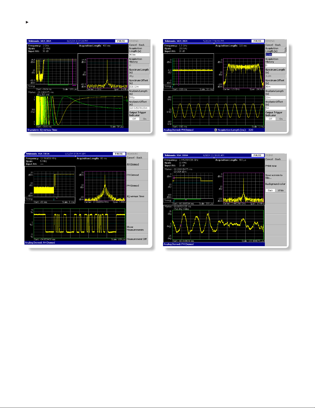
Fundamentals of Real-Time Spectrum Analysis

Primer

www.tektronix.com/rsa

I/Q vs. Time

Transient I/Q vs. Time (Figure 3-10) is another time-domain view

that displays the amplitudes of I and Q as a function of time. This

measurement shows the raw I and Q output signals coming from

the digital down-converter. As a result, this display is not synchro-

nized to any modulation that might be present on the signal being

analyzed, unlike the I/Q vs. Time measurement mode within the

digital demodulation suite.

This measurement can be another useful troubleshooting tool for

expert users, especially in terms of lending insight into frequency

and phase errors and instabilities.

Modulation Domain Measurements

Analog Modulation Analysis

The analog demod mode provides measurements to demodulate and

analyze amplitude modulation (Figure 3-11), frequency modulation

(Figure 3-12), and phase modulation (Figure 3-13). Just like the

time domain measurements, these tools are based on the concept

of multi-domain analysis, and the spectrum and analysis windows

can be positioned anywhere within the block shown in the overview

window.

Figure 3-10: I/Q vs. Time measurement of settling transient.

Figure 3-11: AM demod analysis of a pulsed signal using amplitude shift

keying to encode data.

Figure 3-12: FM demod analysis of a signal being modulated by a sine wave.

Figure 3-13: PM demod analysis showing phase instability over a long burst.

Fundamentals of Real-Time Spectrum Analysis

Primer

Figure 3-14: EVM analysis over time of 16 QAM signal reveals sinusoidal

amplitude distortion.

Digital Modulation Analysis

The digital demod mode can demodulate and analyze many com-

mon digital signals based on phase shift keying (PSK), frequency

shift keying (FSK), and quadrature amplitude modulation (QAM). The

RSA provides a wide range of measurements including: constella-

tion, error-vector magnitude (EVM), magnitude error, phase error,

demodulated I/Q vs. time, symbol table, and eye diagram. To make

these measurements, it is necessary to properly configure variables

such as the modulation type, symbol rate, measurement (receive) filter type and parameter (α/BT), and reference filter type.

The RSA provides a powerful solution for characterizing dynamic

modulated signals by combining the digital demodulation measure-

ments of a VSA with real-time triggering and time-correlated multi-

domain analysis, as illustrated in Figures 3-14, 3-15, and 3-16.

Figure 3-15: Constellation display showing phase instability in a PDC signal.

Figure 3-16: Eye Diagram display showing low magnitude error in a

PDC signal.

www.tektronix.com/rsa

Fundamentals of Real-Time Spectrum Analysis

Primer

www.tektronix.com/rsa

Standards-based Modulation Analysis

The RSA also provides solutions for modulation analysis of many

communications standards such as W-CDMA, HSDPA, GSM/EDGE,

CDMA2000, 1xEV-DO, and more. Figures 3-17 and 3-18 show

examples of standards-based modulation analysis.

Codogram Display

The codogram display (Figure 3-19) of the Real-Time Spectrum

Analyzer adds a time axis to code domain power measurements for

CDMA-based communications standards. Like the spectrogram, the

codogram intuitively shows changes over time.

Figure 3-20 is a W-CDMA codogram display from an RSA. This

particular codogram shows a simulated W-CDMA compressed mode

handoff in which the data rate is momentarily increased to make

room for brief, temporary gaps in the transmission. These gaps

allow dual-mode W-CDMA/GSM user equipment to search for

an available GSM base station while remaining connected to a

W-CDMA Node B.

Figure 3-18: Spectrogram, constellation, EVM, and phase error vs. time of

frequency hopping GSM signal.

Figure 3-20: Codogram measurement of W-CDMA compressed mode.

Figure 3-19: Illustration of the codogram display.

Figure 3-17: Modulation analysis of a W-CDMA handset under closed loop

power control. The constellation display (lower right) shows the error associated with large glitches that occur during level transitions, which can be seen in the power vs. time display (upper left).

www.tektronix.com/rsa

Frequently Asked Questions

Primer

www.tektronix.com/rsa

Chapter 4: Frequently Asked Questions

Real-Time spectrum analysis has existed in some form for many

years, and as the technology enabling this architecture has matured,

the RTSA has become a prevalent tool for a wide variety of applica-

tions that require the ability to characterize RF signals that change

over time. This section addresses several of the frequently asked

questions about real-time spectrum analysis.

What is real-time spectrum analysis?

The fundamental concept of real-time spectrum analysis is the

ability to trigger on an RF signal, seamlessly capture it into memory,

and analyze it in multiple domains. This makes it possible to reliably

detect and characterize RF signals that change over time.

What is real-time bandwidth?

Instead of sweeping across a range of frequencies, the RTSA takes

snapshots of all of the RF energy within the entire span. This span

is known as the real-time acquisition bandwidth. By digitizing the

signal and recording time domain I/Q samples, the RTSA can seam-

lessly capture signals that occur within its real-time bandwidth and

analyze amplitude, frequency, phase, and modulation parameters at

specific points in time.

The real-time bandwidth may be positioned anywhere within the

absolute frequency range of the instrument. For example, the

Tektronix RTSA3308A has a 15 MHz real-time bandwidth that can

be tuned between DC and 8 GHz.

The maximum real-time bandwidth is an important figure of

merit for an RTSA. It is typically limited by the sample rate of the

instrument’s ADCs and the bandwidth over which the instrument’s

IF section has a linear frequency and phase response.

What is real-time seamless capture?

The real-time architecture provides the ability to continuously

capture an RF signal over a long period of time. An uninterrupted

sequence of time domain samples is acquired and stored in the

deep memory of the RTSA. This allows the instrument to create a

time axis to accompany the usual frequency and amplitude axes,

enabling displays such as the spectrogram. Having access to the

raw magnitude and phase representation of the signal also gives the

RTSA the ability to perform complex signal analysis in the frequen-

cy, time, and modulation domains using FFTs and other DSP tech-

niques to process the recorded time-domain samples.

Another important consequence is that as described above, all RF

energy within the real-time acquisition bandwidth is digitized and

recorded simultaneously. Contrast this to the swept spectrum ana-

lyzer, which tunes across the frequency span in narrow steps and

assembles the results to create the spectral display. With the RTSA,

the user can detect and characterize dynamic signals that occur

anywhere within its real-time bandwidth at any time within the block

of seamless time-domain information.

What is meant by “static” and “dynamic” signals?

Static or stationary signals are unchanging signals. Many spectrum

analyzer measurements and communications standards call for

known, well-behaved signals as inputs for the device under test.

Other applications involve observing either basic CW signals or

signals whose modulation type is well known and does not change.

Dynamic signals vary over time. They may change in amplitude,

frequency, phase, or modulation type; or they may disappear and

reappear at regular or unknown intervals. These types of RF signals

can be important to detect and characterize in a variety of applica-

tions ranging from surveillance (where signals appear briefly and

unpredictably) to phase locked loop design (where recovery time

after frequency shifts must comply with design specifications).

Swept spectrum analyzers have difficulty making measurements

on dynamic signals, although they may be able to show some

information about signals that change slowly or predictably.

However, the RTSA is specifically designed to trigger on, capture,

and analyze dynamic signals and transient events.

Why does the RTSA power vs. frequency display look slightly

different from that of a swept SA?

In the RTSA, full spans are acquired continuously, which means that

in some cases screen updates can occur much more quickly than

on a swept spectrum analyzer.

Frequently Asked Questions

Primer

For spans within the real-time bandwidth, the RTSA acquires a

block of data, processes it, then displays the entire range of fre-

quencies at once. Consequently, each screen update is like a new

photographic snapshot of the spectrum. The RTSA display also

changes rapidly when signal amplitude and frequency characteris-

tics change. Dynamic signals might look busy on the RTSA com-

pared to a swept SA since the RTSA is displaying the signal

changes as they actually happen.

With a swept SA, a filter equal to the width of the RBW filter setting

moves through the spectrum. Signal amplitude at any frequency in

the span is measured only when the sweeping window passes

through that frequency. This window may be just a few percent of

the total span but it is easy to locate the instantaneous frequency of

the sweep. However, it is impossible to know whether an event such

as a transient may be occurring elsewhere.

For spans exceeding its real-time bandwidth, the RTSA acquires and

processes one segment of the span at a time, much like a swept

SA. Its behavior in this mode is similar to the swept SA, although

there may be significant speed differences due to the different

methods of implementing RBW filters (usually analog in a swept SA,

digital in the RTSA). For very wide measurement spans, the RTSA

tends to be faster for narrow RBW settings, and the swept SA tends

to be faster for wide RBW settings.

Applying a resolution bandwidth filter in standard SA mode

makes the measured signals look different. Why?

The RTSA has all of its RBW filters implemented in DSP. Compared

to common analog spectrum analyzers, the shape factors on these

filters can be much steeper, producing a narrower appearance in

the spectral content.

The steep RBW shape factor is an improvement over swept spectrum

analyzers because low-level signals close to the carrier can be

resolved. Phase noise is easier to see because it doesn’t hide under

a wide-RBW filter skirt.

Noise looks different on an RTSA. Can noise power be meas-

ured accurately?

In real-time acquisition modes, the RTSA takes rapid snapshots of

the input RF signal. If it is to characterize fast changes in these RF

signals, it must necessarily analyze the incoming signals over very

short windows of time (frames). Therefore, it shows exactly the

noise character of the spectrum represented in each frame. The

traditional swept spectrum analyzer must sweep slowly, and there-

fore it is forced to average the noise as it sweeps across the entire

frequency span. This longer “analysis time” of the swept SA is why

it looks different than the display of the RTSA.

The noise bandwidth of the RTSA is very predictable since the FFT

bin width is a known value determined by DSP. Therefore noise

power spectral density can be measured accurately in any real-time

span of the RTSA.

In standard SA acquisition modes, video filtering and display

averaging are available to process the noise. In this case, display

averaging will produce a noise signal shape that is very similar to

that of a swept spectrum analyzer.

What is noise bandwidth?

Noise bandwidth (NBW) is the RTSA equivalent to the resolution

bandwidth (RBW) of a swept spectrum analyzer. In its real-time

modes, the RTSA’s frequency resolution is expressed by its NBW.

When it is in standard SA mode (which emulates a swept SA),

the RTSA offers the same adjustable RBW settings as a traditional

swept SA.

The NBW of a filter is determined by integrating the filter’s normal-

ized transfer function over all frequencies from zero to infinity, and

relating the power the filter will transfer to an ideal 1Hz brick wall

(rectangular) filter with a noise bandwidth of 1Hz.

Swept SAs typically use RBW filters that are characterized for noise

bandwidth and corrected internally. Knowing the noise bandwidth

is essential for measurements in which the signal itself is noise,

or where it has noise-like power distribution (as in a CDMA

transmission).

www.tektronix.com/rsa

Frequently Asked Questions

Primer

www.tektronix.com/rsa

RTSA’s use BH4B filtering in its real-time mode. Since filtering is

done by DSP, it is possible to calculate the actual noise bandwidth

and display it on the screen with the other instrument settings

and measurement results. This method provides accurate noise

measurements.

How does span affect time domain resolution of the RTSA?

As described in Chapter 3, the span setting of the RTSA determines

the effective sample rate for the time domain data that is stored in

the memory of the instrument. Table 4-1 illustrates the impact of

increasing and decreasing the span.

Span Sample Decimation Effective Time Domain Spectrogram Maximum

Rate Sample Resolution Time Record

Rate Resolution Length

15 MHz 51.2 MS/s 2 25.6 MS/s 39.0 ns 40 usec 2.56 sec

10 MHz 51.2 MS/s 4 12.8 MS/s 78.1 ns 80 usec 5.12 sec

5 MHz 51.2 MS/s 8 6.4 MS/s 156 ns 160 usec 10.2 sec

2 MHz 51.2 MS/s 16 3.2 MS/s 312 ns 320 usec 20.5 sec

1 MHz 51.2 MS/s 32 1.6 M/s 625 ns 640 usec 40.0 sec

500 KHz 51.2 MS/s 64 800 KS/s 1.25 us 1.28 msec 81.0 sec

200 KHz 51.2 MS/s 160 320 KS/s 3.13 us 3.20 msec 205 sec

100 KHz 51.2 MS/s 320 160 KS/s 6.25 us 6.40 msec 410 sec

50 KHz 51.2 MS/s 640 80 KS/s 12.5 us 12.8 msec 13.7 min

20 KHz 51.2 MS/s 1600 32 KS/s 31.3 us 32 msec 34.1 min

10 KHz 51.2 MS/s 3200 16 KS/s 62.5 us 64 msec 68.2 min

5 KHz 51.2 MS/s 6400 8 KS/s 125 us 128 msec 136.6 min

2 KHz 51.2 MS/s 16000 3.2 KS/s 312 us 320 msec 5.69 hour

1 KHz 51.2 MS/s 32000 1.6 KS/s 625 us 640 msec 11.4 hour

500 Hz 51.2 MS/s 64000 800 S/s 1.25 ms 1.28 sec 22.8 hour

200 Hz 51.2 MS/s 160000 320 S/s 3.13 ms 3.2 sec 2.37 day

100 Hz 51.2 MS/s 320000 160 S/s 6.25 ms 6.4 sec 4.74 day

Table 4-1: RTSA span selection and resulting time resolution effects. (Tektronix RSA3300A Series and WCA200A Series)

Frequently Asked Questions

Primer

Span Sample Decimation Effective Frequency Noise Bandwidth

15 MHz 51.2 MS/s 2 25.6 MS/s 25 kHz 42.7 kHz

10 MHz 51.2 MS/s 4 12.8 MS/s 12.5 kHz 21.4 kHz

5 MHz 51.2 MS/s 8 6.4 MS/s 6.25 kHz 10.7 kHz

2 MHz 51.2 MS/s 16 3.2 MS/s 3.13 kHz 5.34 kHz

1 MHz 51.2 MS/s 32 1.6 M/s 1.56 kHz 2.67 kHz

500 KHz 51.2 MS/s 64 800 KS/s 781 Hz 1.33 kHz

200 KHz 51.2 MS/s 160 320 KS/s 313 Hz 534 Hz

100 KHz 51.2 MS/s 320 160 KS/s 156 Hz 267 Hz

50 KHz 51.2 MS/s 640 80 KS/s 78.1 Hz 133 Hz

20 KHz 51.2 MS/s 1600 32 KS/s 31.3 Hz 53.4 Hz

10 KHz 51.2 MS/s 3200 16 KS/s 15.6 Hz 26.7 Hz

5 KHz 51.2 MS/s 6400 8 KS/s 7.81 Hz 13.3 Hz

2 KHz 51.2 MS/s 16000 3.2 KS/s 3.13 Hz 5.34 Hz

1 KHz 51.2 MS/s 32000 1.6 KS/s 1.56 Hz 2.67 Hz

500 Hz 51.2 MS/s 64000 800 S/s 781 mHz 1.33 Hz

200 Hz 51.2 MS/s 160000 320 S/s 312 mHz 534 mHz

100 Hz 51.2 MS/s 320000 160 S/s 156 mHz 267 mHz

Table 4-2: RTSA span selections and resulting frequency domain effects. (Tektronix RSA3300A Series and WCA200A Series)

Rate Sample Resolution (NBW)

Rate (FFT bin width)

How does span affect frequency domain resolution of

the RTSA?

Digital down conversion and decimation have equally significant

effects on the frequency domain resolution of the RTSA. The

frequency resolution of a real-time measurement is defined by the

width of the FFT bin and by the NBW for noise-like signals. Table 4-2

illustrates the impact of increasing and decreasing the span.

How does the general RF performance of RTSA compare to a

swept spectrum analyzer?

The RTSA generally compares favorably with modern swept SAs that

use digital IF sections. Here is an overview of the primary areas in

which either type of analyzer can introduce measurement errors.

Real-Time Measurements: The swept spectrum analyzer has

effectively no real-time capability, and consequently tends to

introduce large errors for transient signals. The RTSA is optimized to

trigger on, capture, and analyze transient or time-varying signals.

Distortion: Distortion processes for the swept SA and the RTSA are

equivalent through the RF converter. After the RF converter, distor-

tion in the RTSA is dependent on the ADC resolution as well as the

bit width of the subsequent DSP operations. The fundamentals of

ADC technology dictate tradeoffs between distortion performance

and bandwidth. The RTSA is designed to achieve wide real-time

bandwidths and consequently has less dynamic range than some

high performance conventional swept SAs.

Spurs: Spurs may be generated in the wideband ADC, DDC, and

FFT processing steps. However, all of these factors can be held to

levels such that the net spurious performance of the RTSA is typi-

cally equivalent to that of swept SAs.

Thermal Noise and Phase noise: The dominant thermal noise and

phase noise mechanisms are similar for both RTSAs and swept SAs.

www.tektronix.com/rsa

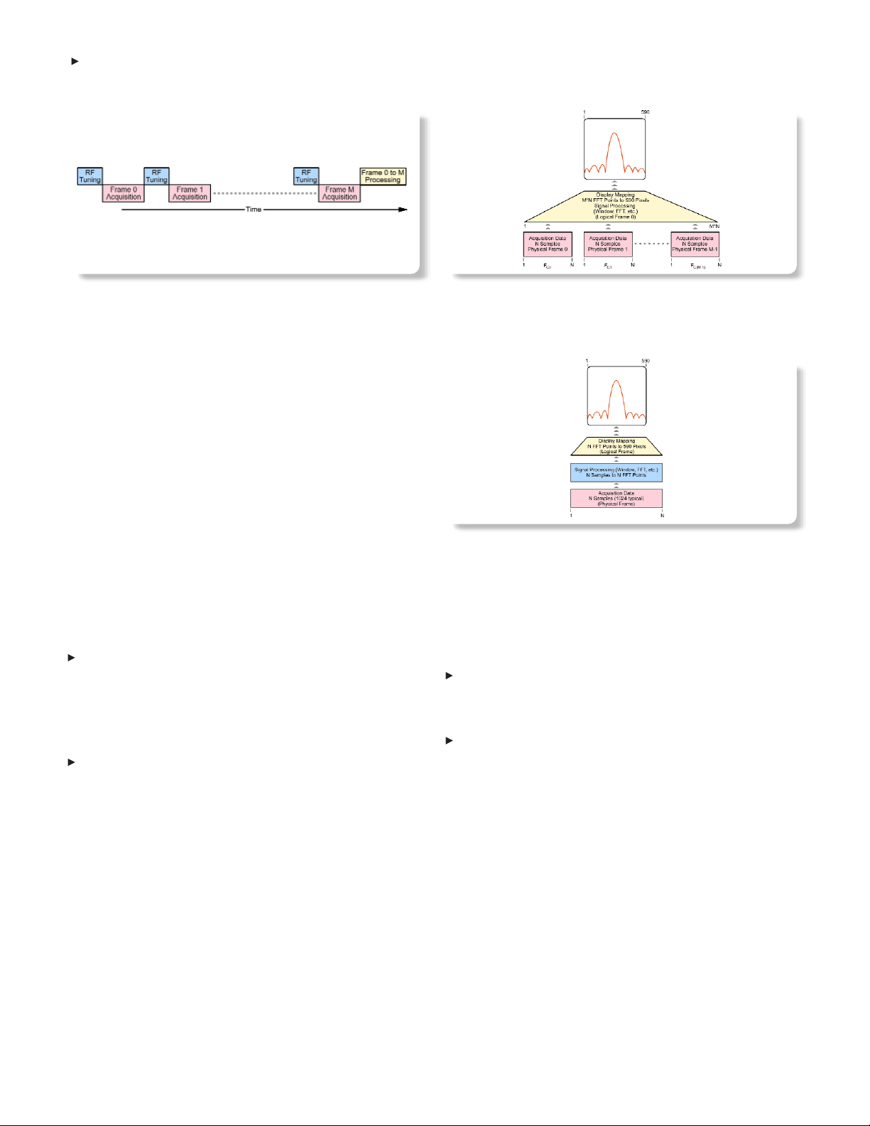
Frequently Asked Questions

Primer

www.tektronix.com/rsa

Amplitude Flatness: The RF converter amplitude flatness is

equivalent for RTSA and swept SA architectures. Because the RTSA

relies on a wide-band IF filter and the digital filters in the DDC are

optimized for transition-band performance, RTSA design requires

special attention to counteract any deviations from flat response.

In practice, the RTSA’s amplitude flatness performance approxi-

mates that of swept SAs.

Detector and Log Errors: Neither the RTSA nor the modern swept

SA is troubled by the detector and logarithmic errors found in older

analog spectrum analyzers. Both of these modern instrument

families use ADCs and DSP to accomplish detection and log scaling.

How does the RTSA make measurements in spans greater than

the real-time bandwidth?

There are two different acquisition modes used in the Tektronix

RTSA3300A Series and WCA200A Series:

Block acquisition mode (as explained Chapters 1 and 2) is the

method that is used for most Real-Time Spectrum Analyzer

measurements including real-time spectrum analysis, time

domain analysis, and modulation analysis. In this mode, the span

cannot exceed the maximum real-time bandwidth.

Standard SA acquisition mode is the method that is used to

emulate the frequency domain measurements of a traditional

swept spectrum analyzer. In this mode, the span can exceed the

maximum real-time bandwidth.

Standard SA acquisition mode allows the analyzer to make

measurements in spans larger than the real-time bandwidth in

two specific measurement modes: standard SA mode and SA with

spectrogram mode. Note that in these cases the instrument is not

making seamless real-time measurements. Instead of acquiring a

block of contiguous time domain samples, acquisitions are made on

a frame-by-frame basis with gaps in between frames as shown in

Figure 4-1. This mode uses two different data structures:

Logical Frame: a set of 590 display points used to represent

one span of frequencies. The span of a logical frame may

exceed the real-time bandwidth.

Physical Frame: a set of N time-domain samples used to

produce one FFT. For spans less than the real-time bandwidth, a

single physical frame equates to a single logical frame. For

spans greater than the real-time bandwidth, multiple physical

frames map into a single logical frame.

For spans exceeding the real-time bandwidth, the span is measured

using several physical frames acquired as the RF converter is tuned

through the input spectrum in 10 MHz steps. One physical frame is

acquired per tuning step. This acquisition sequence is shown in

Figure 4-1, and the data mapping is shown in Figures 4-2 and 4-3.

Figure 4-1: Standard SA mode signal acquisition and processing.

Figure 4-2: Standard SA mode data mapping for spans that exceed the

real-time bandwidth. There are N samples per physical frame, M physical frames, and 1 logical frame.

Figure 4-3: Standard SA mode data mapping for spans less than the

real-time bandwidth.

Frequently Asked Questions

Primer

How does the RSA Series front panel differ from a swept SA?

Are there any similarities?

The RSA has many of the same controls as its swept predecessors:

Center Frequency, Span, Reference Level (Amplitude), RF

Attenuation, and other front panel buttons will be very familiar to

engineers who have used swept SAs in the past. The RSA also has

a standard SA mode where the instrument provides a power vs.

frequency display and behaves almost identically to a swept SA.

In standard SA mode, a few RSA parameters look or behave differ-

ently from those on swept SAs. Sweep time for a swept spectrum

analyzer is equivalent to frame length in an RSA. Frame length

depends on span size, number of points acquired, and sample rate.

The user can control span size and sometimes the number of points

acquired.

In other modes, the RSA has many new controls that support the

various real-time measurements that cannot be made with a swept

SA. The acquisition timing control allows the user to set how much

real-time data to acquire. Acquisitions can be as short as one frame

of data or as long as the hardware memory capacity permits. Other

new controls pertain to FFT processing. These include number of

FFT points, windowing function type selection, and RBW filter types.

When should I use a RTSA? When should I use a swept SA?

No single analyzer will ever be the best solution for every RF

measurement challenge. In fact, many common measurements can

be performed with equal effectiveness using either a swept SA or

RTSA. In many cases, the RTSA is a more versatile tool, since it

provides real-time measurements in addition to basic frequency

domain measurements.

Measurements of transient and dynamic signals that change

over time – RTSA

Real-time triggering, seamless capture, and in-depth signal

analysis – RTSA

Correlation of time, frequency, and modulation domain

events — RTSA

Modulation analysis for complex communications

standards — RTSA or VSA

Basic parametric frequency domain measurements — RTSA or

swept SA

Static signal measurements requiring extremely high dynamic

range — swept SA

The unique triggering controls of the RSA are also new to the field

of spectrum analysis. Triggering functions such as frequency mask

triggering are simply not possible in a conventional swept SA. The

RSA provides precise control over triggering parameters including

both frequency and amplitude.

www.tektronix.com/rsa

Glossary

Primer

www.tektronix.com/rsa

Chapter 5: Glossary

Acquisition

An integer number of time-contiguous frames; a block.

Acquisition Time

The length of time represented by one acquisition. Same as

block length.

Amplitude

The magnitude of an electrical signal.

Amplitude Modulation (AM)

The process in which the amplitude of a sine wave (the carrier) is

varied in accordance with the instantaneous voltage of a second

electrical signal (the modulating signal).

Analysis Time

A subset of time-contiguous samples from one block, used as input

to an analysis view.

Analysis View

The flexible window used to display real-time measurement results.

Block

An integer number of time-contiguous frames.

Carrier

The RF signal upon which modulation resides.

Carrier Frequency

The frequency of the CW component of the carrier signal.

Center Frequency

The frequency corresponding to the center of a frequency span of

the analyzer display.

Codogram

Code channel vs. time vs. power display where the CDMA code

channel is represented on x-axis and time respectively on the y-

axis. The power level is expressed by the color.

CW Signal

Continuous wave signal – a sine wave.

dBfs

A unit to express power level in decibels referenced to full scale.

Depending on the context, this is either the full scale of the display

screen or the full scale of the ADC.

dBm

A unit to express power level in decibels referenced to 1 milliwatt.

dBmV

A unit to express voltage levels in decibels referenced to 1 millivolt.

Decibel (dB)

Ten times the logarithm of the ratio of one electrical power to

another.

Display Line

A horizontal or vertical line on a waveform display, used as a refer-

ence for visual (or automatic) comparison with a given level, time, or

frequency.

Distortion

Degradation of a signal, often a result of nonlinear operations,

resulting in unwanted frequency components. Harmonic and inter-

modulation distortion are common types.

Dynamic Range

The maximum ratio of the levels of two signals simultaneously pres-

ent at the input which can be measured to a specified accuracy.

FFT

Fast Fourier Transform – a mathematical process to calculate the

frequency spectrum of a discrete number of time domain sample

points.

Frame

A series of time-contiguous samples; used to calculate a single fre-

quency spectrum.

Frame Length

The amount of time represented by the time domain samples within

a frame; a function of the number of sample points and the sam-

pling rate.

Frequency

The rate at which a signal oscillates, expressed as hertz or number

of cycles per second.

Frequency Domain View

The representation of the power of the spectral components of a

signal as a function of frequency; the spectrum of the signal.

Glossary

Primer

Frequency Drift

Gradual shift or change in displayed frequency over the specified

time, where other conditions remain constant. Expressed in hertz

per second.

Frequency Mask Trigger

A flexible real-time trigger based on specific events that occur in

the frequency domain.

Frequency Modulation (FM)

The process in which the frequency of an electrical signal (the carri-

er) is varied according to the instantaneous voltage of a second

electrical signal (the modulating signal).

Frequency Range

The range of frequencies over which a device operates, with lower

and upper bounds.

Frequency Span

A continuous range of frequencies extending between two

frequency limits.

Marker

A visually identifiable point on a waveform trace, used to extract a

readout of domain and range values represented by that point.

Modulate

To vary a characteristic of a signal, typically in order to transmit

information.

Noise

Unwanted random disturbances superimposed on a signal which

tend to obscure it.

Noise Floor

The level of noise intrinsic to a system that represents the minimum

limit at which input signals can be observed; ultimately limited by

thermal noise (kTB).

Noise Bandwidth (NBW)

The exact bandwidth of a filter that is used to calculate the absolute

power in dBm/Hz.

Real-Time Bandwidth

The frequency span over which real-time seamless capture can be

performed, which is a function of the digitizer and the IF bandwidth

of a Real-Time Spectrum Analyzer.

Real-Time Seamless Capture

The ability to acquire and store an uninterrupted series of time

domain samples that represent the behavior of an RF signal over a

long period of time.

Real-Time Spectrum Analysis

Measurement technique based triggering on an RF signal, seam-

lessly capturing it into memory, and analyzing it in the frequency,

time, and modulation domains.

Reference Level

The signal level represented by the uppermost graticule line of the

analyzer display.

Resolution Bandwidth (RBW)

The width of the narrowest filter in the IF stages of a spectrum ana-

lyzer. The RBW determines the analyzer’s ability to resolve closely

spaced signal components.

Sensitivity

Measure of a spectrum analyzer’s ability to display minimum level

signals, usually expressed as displayed average noise level (DANL).

Spectrogram

Frequency vs. time vs. amplitude display where the frequency is

represented on x-axis and time on the y-axis. The power is

expressed by the color.

Spectrum

The frequency domain representation of a signal showing the power

distribution of its spectral component versus frequency.

Spectrum Analysis

Measurement technique for determining the frequency content of an

RF signal.

Vector Signal Analysis

Measurement technique for charactering the modulation of an RF

signal.

www.tektronix.com/rsa

Acronym Reference

Primer

www.tektronix.com/rsa

Acronym Reference

ADC: Analog-to-Digital Converter

AM: Amplitude Modulation

BH4B: Blackman-Harris 4B Window

CCDF: Complementary Cumulative Distribution Function

CDMA: Code Division Multiple Access

CW: Continuous Wave

dB: Decibel

dBfs: dB Full Scale

DDC: Digital Down Converter

DSP: Digital Signal Processing

EVM: Error Vector Magnitude

FFT: Fast Fourier Transform

FM: Frequency Modulation

FSK: Frequency Shift Keying

IF: Intermediate Frequency

I/Q: In-Phase / Quadrature

LO: Local Oscillator

NBW: Noise Bandwidth

OFDM: Orthogonal Frequency Division Multiplexing

PM: Phase Modulation

PSK: Phase Shift Keying

QAM: Quadrature Amplitude Modulation

RBW: Resolution Bandwidth

RF: Radio Frequency

rms: Root Mean Square

RSA: Tektronix' Real-Time Spectrum Analyzer

RTSA: Real-Time Spectrum Analyzer

SA: Spectrum Analyzer

VSA: Vector Signal Analyzer

www.tektronix.com/rsa

Contact Tektronix:

ASEAN / Australasia / Pakistan

Austria

Belgium

Brazil & South America

Central Europe & Greece

Denmark

Finland

France & North Africa

Germany

Hong Kong

Mexico, Central America & Caribbean

The Netherlands

People’s Republic of China

Poland

Republic of Korea

Russia, CIS & The Baltics

South Africa

Sweden

Taiwan

United Kingdom & Eire

USA (Export Sales)

For other areas contact Tektronix, Inc. at: 1 (503) 627-7111

(65) 6356 3900

+43 2236 8092 262

+32 (2) 715 89 70

55 (11) 3741-8360

Canada

1 (800) 661-5625

+43 2236 8092 301

+45 44 850 700

+358 (9) 4783 400

+33 (0) 1 69 86 80 34

+49 (221) 94 77 400

(852) 2585-6688

India

(91) 80-22275577

Italy

+39 (02) 25086 1

Japan

81 (3) 6714-3010

52 (55) 56666-333

+31 (0) 23 569 5555

Norway

+47 22 07 07 00

86 (10) 6235 1230

+48 (0) 22 521 53 40

82 (2) 528-5299

+358 (9) 4783 400

+27 11 254 8360

Spain

(+34) 901 988 054

+46 8 477 6503/4

886 (2) 2722-9622

+44 (0) 1344 392400

USA

1 (800) 426-2200

1 (503) 627-1916

www.tektronix.com/rsa

For Further Information

Tektronix maintains a comprehensive, constantly expanding collection of application notes, technical briefs and other resources to help engineers working on the cutting edge of technology. Please visit

www.tektronix.com

Copyright © 2004, Tektronix, Inc.All rights reser ved. Tektronix products are covered by U.S. and foreign patents, issued and pending. Information in this publication supersedes that in all previously published material. Specification and price change privileges reserved. TEKTRONIX and TEK are registered trademarks of Tektronix, Inc.All other trade names referenced are the ser vice marks, trademarks or registered trademarks of their respective companies. 09/04 HA/WOW 37W-17249-0

Tektronix Fundamentals Of Real-Time Spectrum Analysis User Manual

Specifications and Main Features

Frequently Asked Questions

User Manual