Tektronix fundamentals of analysis schematic

Download

TCZL/

LlX

SPECTRUM

ANALYZERS

26W-5360

FUNDAMENTALS OF

SPECTRUM ANALYSIS

Tektronix

COMMITTED TO

EXCELLENCE

CONTENTS: Preface

Introduction

Primary Controls

...................................................

...............................................

Nature of Measurement

Types of Measurement

.....................................

......................................

...........................................

Amplitude

Scale Factor (Vertical Display) Reference Level

................................................

...............................

..........................................

Typical Spectrum Analyzer Controls Photo

Frequency

Frequency Control Span Control Resolution Bandwidth

Secondary Controls

Sweep Video Filter

Digital Storage Frequency Range Phase Lock Preselector

................................................

........................................

............................................

.....................................

.........................................

Time...............................................

...............................................

.............................................

..........................................

...............................................

.......................

1 1

1 2

3 4 6 6 6 6

7 8 8 9 9 9

Applications

Amplitude Modulation

Harmonic Distortion Intermodulation Distortion

Tracking Generator

Pulsed Noise

Antenna Sweeps

Glossary

...............................................

.......................................

..................................

..............................:..........

RF(Radar)

..........................................

Measurements........................................

...........................................

..................................................

Fundamentals of Spectrum

Analysis

was written by

Engineering Operations Manager, Frequency Domain

Bill

Benedict,

Instruments,

Tektronix, Inc.

11 11 12 14 15

Preface

This handbook explains the fundamentals, or basics, of spectrum analysis. It describes the essential

controls and how to use them, how

to make elementary measurements,

and how to interpret the display.

There are other articles available

from Tektronix, Inc. and others, that describe in more detail the operation of an analyzer and the interpretation of the display. After reading this handbook, an individual familiar with basic electronics and primary electronic communication theory will be able to make basic measure-

ments with an analyzer.

For the best results, use an analyzer

when reading the text, especially the section on Primary Controls. The

material will be much more mean-

ingful. Trying to duplicate the photos

is the most effective way to understand the function of each control.

A multi-function signal generator will

provide most of the signals used in the photos. Gaining the basic know-

ledge of how to use a Spectrum

Analyzer will make it easier to switch from one model analyzer to

another.

This text will not discuss all the controls of an analyzer as many of them

are for special functions and will vary

between analyzers and manufac-

turers. The operator's manual for a

particular analyzer should be consulted regarding the exact opera-

tion of all controls.

electrical signal during the mea-

surement interval with respect to

time. Likewise, a Spectrum Analyzer

permits observation of the amplitudes

and frequencies of the various dis-

crete sinusoidal signals during the

measurement interval. In both cases, the results are displayed on a cathode-ray tube (crt) with the vertical axis being the amplitude scale and the horizontal axis being the time

scale for an oscilloscope or the fre-

quency axis for a Spectrum Analyzer.

Figures waveforms as displayed on both an

oscilloscope and a Spectrum Ana-

lyzer.

2, and 3 show various

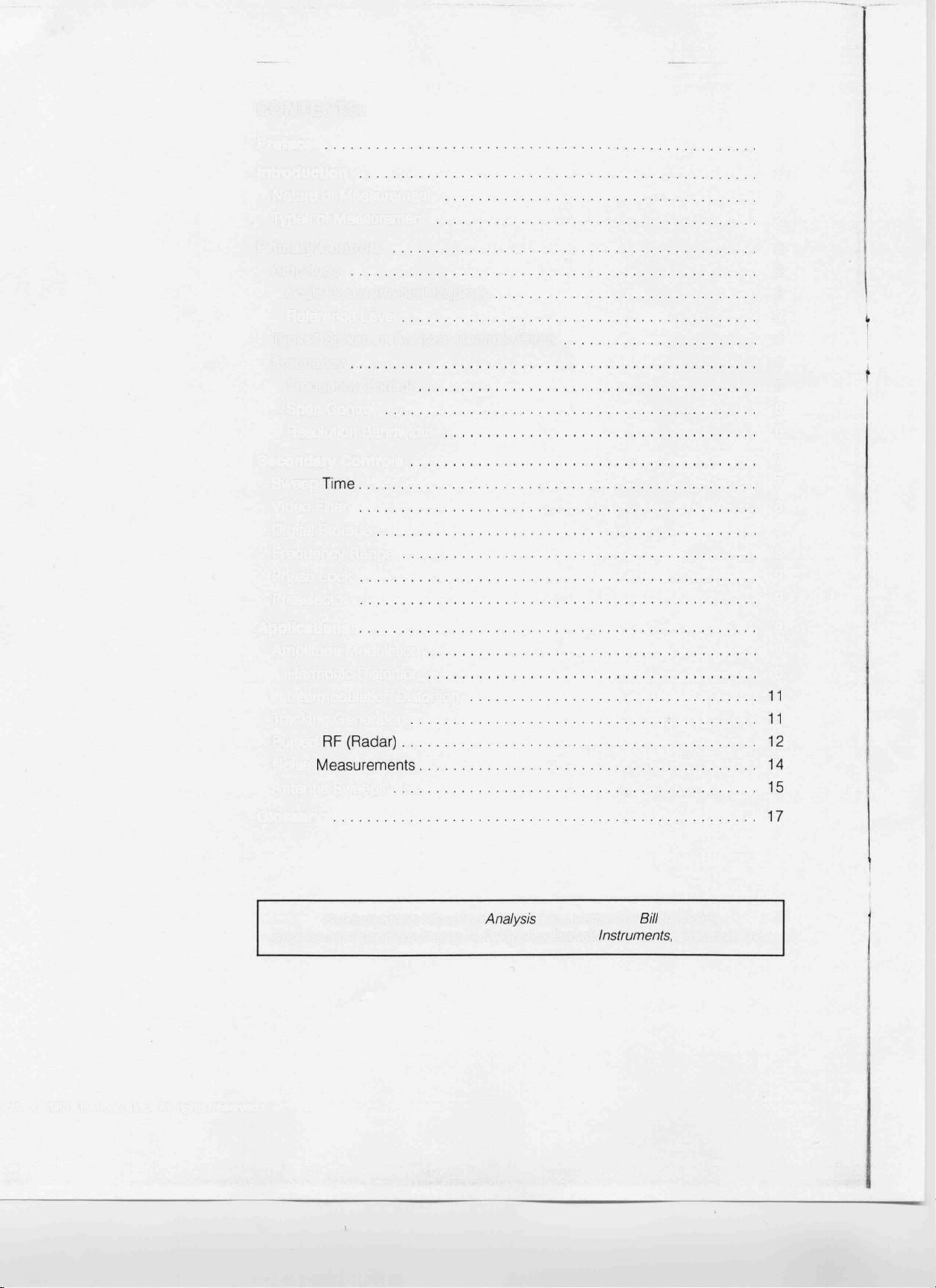
In the first example, a sine wave is displayed. The oscilloscope displays

the

peak-to-peak

voltage (vertical axis)

of the signal with respect to time

(horizontal axis). The Spectrum An-

alyzer shows the same sine wave

Oscilloscope Waveform: 3 MHz Sine Wave

Figure 1.

where the positive peak (vertical axis)

indicates the amplitude of signal and

the single signal (horizontal axis) indicates there is only one frequency or sine wave present. [You will note the presence of a zero hertz marker. It is present due to system design of a Spectrum Analyzer and is present regardless of the input signal. All signals to the left of the zero hertz marker are not negative frequencies as one might think; they are images or reflections of those signals to the right of the zero hertz

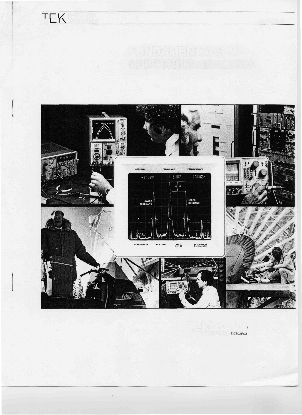
The second example (Fig. 2) is a

modulated carrier where both the modulation frequency and carrier

frequency can be determined. The

Spectrum Analyzer indicates the carrier as the larger signal and the

modulation as the two smaller sig-

nals (upper and lower sidebands).

Spectrum Analyzer Waveform: 3 MHz

Sine Wave

marker].

Introduction

Nature of Measurement

All electrical waveforms or signals

are composed of a combination of

sinusoidal signals of varying amplitudes and frequencies. The combination of sine waves can be observed in the time domain with an oscilloscope, or in the frequency domain with a Spectrum Analyzer. The oscilloscope enables observation of

the amplitude and shape of an

Oscilloscope Waveform: Modulated Carrier at 1 MHz, 15 kHz Modulation

Figure 2.

Spectrum Analyzer Waveform: Modulated

Carrier at 1 MHz,

kHz Modulation

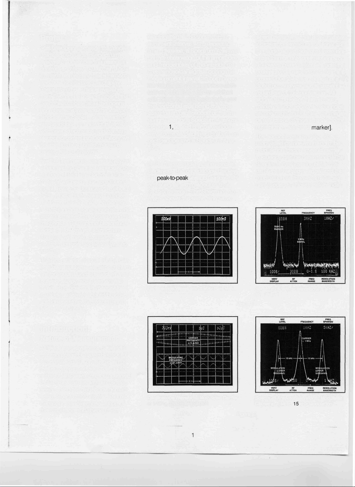
The third example (Fig. 3) shows the signal appearing on the oscilloscope as a square wave. The Spectrum Analyzer displays a "fundamental"

sine wave at the same frequency as

the square wave and the other frequencies of diminishing amplitude

(as the frequency increases) that

make up a square wave. These other frequencies are identified as the

3rd,

5th,

7th,

etc.

(odd)

har-

monics of the fundamental fre-

quency.

Types of Measurements

Composite voltage waveforms are

displayed by an oscilloscope. The

Spectrum Analyzer, as the name

implies, analyzes the composite

form and displays the individual fre-

quency components and the relative power each component contributes

to the total waveform.

Since the Spectrum Analyzer has this characteristic, it is well suited for work that involves oscillators, RF carriers, RF spectrum surveillance, etc. With an analyzer, it is possible to observe:

wave-

• an oscillator

• RF carrier

• amount and frequency of modulation

• unexpected modulation

• carrier suppression in single

sideband radio

• harmonic level of oscillators and

RF carriers

With a sweeping oscillator or "Tracking Generator", filter response, amplifier frequency response, and

antenna standing wave ratio (SWR) can all be checked, along with other

measurements described in the Ap-

plications section dealing with the

Tracking Generator.

Primary Controls

(Refer to front panel photo on pages

4 and 5 for typical Spectrum

Analyzer controls).

Oscilloscope Waveform: 100 kHz Square Wave

Amplitude

The Spectrum Analyzer has two

major amplitude controls. The first controls the scale factor

dB/div) and the second determines

what input signal amplitude is necessary to produce a signal display

up to the top line on the crt, which

is called the Reference Level.

Scale Factor (Vertical Display)

Most oscilloscope graticules are

divided vertically into eight major

divisions. Each major division is further divided into five minor divisions. Thus, a signal of one minor division

in amplitude can be accurately

measured and another signal of

eight divisions in amplitude can be

measured and compared to determine the larger one as being

div (5 minor div/div)

1 minor division

= 40 times greater than

the smaller signal.

To determine this ratio in dB, use

= 20 log ^ = 32dB.

Since many Spectrum Analyzers are

capable of displaying ratios of 80 dB on screen, either a different scale factor is required or a crt display with 2,000 major vertical divisions is required! The obvious solution is to

use a logarithmic scale of 10 dB/div

(volts/div

Figure 3.

Spectrum Analyzer Waveform: 100 kHz

Square Wave

with the standard eight division screen to display 80 dB of range.

As an example, with 80 dB of on-

screen range, two signals can be

measured simultaneously; one of 1 W

( + 30 dBm) and the other of 0.01

(-50

dBm). That is a voltage ratio

10,000:1 , far greater than the

/WV

40:1

ratio possible with the oscilloscope. Before going further, note the basic

equations that can be used to con-

vert to dB,

dBm,

dBV, and

dBmV.

Once you begin to use the Spectrum

Analyzer, you will find that most mea-

surements will be in dB or dBm and

no conversion will be necessary. It is

not important that you conquer these equations before going further.

Signal ratios are expressed in dB:

or1 0 log

Power into a known load (50, 75,

600 ohms, etc.) is expressed in:

dBm

* (at specified impedance)

dBV = 20

dBmV = 20log

* (volts are

The obvious problem with having a

RMS

Power (1)

= 10 log

log

volts)

Power*

1 V

1 mV

scale factor that allows such a large range of signals on screen simultaneously is that two signals appear-

ing close in amplitude may in reality vary significantly in amplitude. As an

example, assume there is one signal

of 1

and another signal of 2

power. Using the equations, it is

apparent they are

+ 30 dBm MAX

STEP

ATTENUATOR

OPTIMUM INPUT

LEVEL

-30

( + 13 dBm

dBm

MAX)

10 log

1 mW

=10log2 =

apart in amplitude, or 1.5 minor divi-

sions with a scale factor of 10 dB/div.

To allow accurate measurements of signals of close amplitudes, an ana-

lyzer typically has a Display Mode of

2 dB/div where, as in the previous example of two signals being 3 dB apart

(2X),

the display would indicate

1.5 major divisions of separation. A

third common display mode is linear

scale factor, where the

RMS

value

of the signal is displayed with a cali-

bration of

volts/div.

Reference Level

The Reference Level is one of the

three main controls of a Spectrum Analyzer. The purpose of this control is to obtain an adequate display of signal amplitude on screen. This

control sets the level of the signal

necessary to produce a full-screen deflection (i.e., the top of the screen is the Reference Line). Thus, if the Reference Level control is set for 0 dBm with a Vertical Display of

dB/div, a 0 dBm signal would rise

to the top

-20

crt

graticule marking. A

dBm signal would be 2 divi-

sions down from the top [0 dBm

- 2 div

(1 0 dB/div) = - 20

dBm].

Some analyzers separate the Refer-

ence Level control into two individ-

ual controls. Together they represent the Reference Level, but separately each controls an individual section

of the analyzer. The two independent sections of the analyzer are the RF

Attenuator control and the IF Gain control.

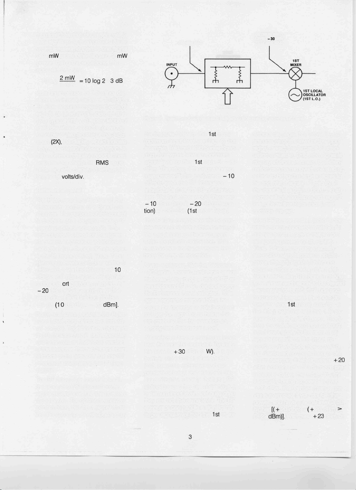
The RF Attenuator control selects

the amount of RF attenuation the

signal experiences just after it enters the analyzer. For optimum analyzer performance, the input signal must be attenuated to a level specified by

CONTROL

Figure 4. Spectrum Analyzer Input Indicating Point of Optimum Input Level.

the manufacturer for the

(optimum input level, see Fig. 4). For

example, Tektronix 490 Series Spectrum Analyzers have an optimum signal level for the dBm. Therefore, if the signal being

measured with the analyzer is

dBm in level, the RF attenuator should be set for 20 dB of attenua-

tion. The first mixer would then see:

-10

dBm (input)

tion)

= -30 dBm

-20

(1st

The IF Gain control selects the proper amount of gain within an amplifier stage to keep the instrument within amplitude calibration. This

control does not have any restrictions for proper operation.

Some analyzers, like the Tektronix 490 Series, contain a microprocessor

that selects the proper ratio of RF attenuation and IF gain, depending on the Reference Level selected. This

eases operator responsibility, be-

cause the operator is only required to keep the signal at or below the top graticule line by selecting an

appropriate Reference Level.

All analyzers have a maximum input

level that must be observed. Typically,

this level is

+30

dBm (1

tremely important to observe this

limit, because extensive and ex-

pensive damage may occur to the

input circuitry. Usually, both the RF

attenuator and the 1 st mixer have a

maximum input level, and quite often

they are not the same level. The RF

attenuator can handle a significantly

larger signal level than the

1st

mixer

1st

mixer of -30

dB (attenua-

mixer level).

W).

It is ex-

1st

-10

mixer

without damage. Therefore, if you are unsure of the level of the input signal, select the largest RF attenuation available. Once the signal is displayed on the screen, the atten-

uation can be removed one step at

a time to bring the largest signal to

the top of the screen. Typically, if

the input is less than 0 dBm, the analyzer will not be damaged regardless of how the Reference Level

controls are set.

Most RF power meters indicate the total amount of power available at the head of the power meter from

all signals present on the cable. Thus, if there are many discrete

sinusoidal signals present on the

cable, the amplitude of any one

signal cannot be determined with the power meter. The Spectrum Analyzer allows each signal to be viewed separately for both amplitude and frequency. However, the input (at-

tenuator and

1st

mixer) circuitry is

like the power meter in that it is exposed to all signals present. Therefore, the rules regarding maximum input level apply to the sum of all signals present on the input, re-

gardless of whether they are all be-

ing displayed on the screen or not.

As an example, if two signals of

dBm and one of -50 dBm are sent on a cable, the input circuitry

is actually being exposed to over

+ 23 dBm. Remember (from a pre-

vious example), if you double the

power, you have a signal level 3 dB

higher

[(+

20 dbm) +

( + 23

dBm)].

With over

20 dBm)

+23

+20

pre-

dBm on

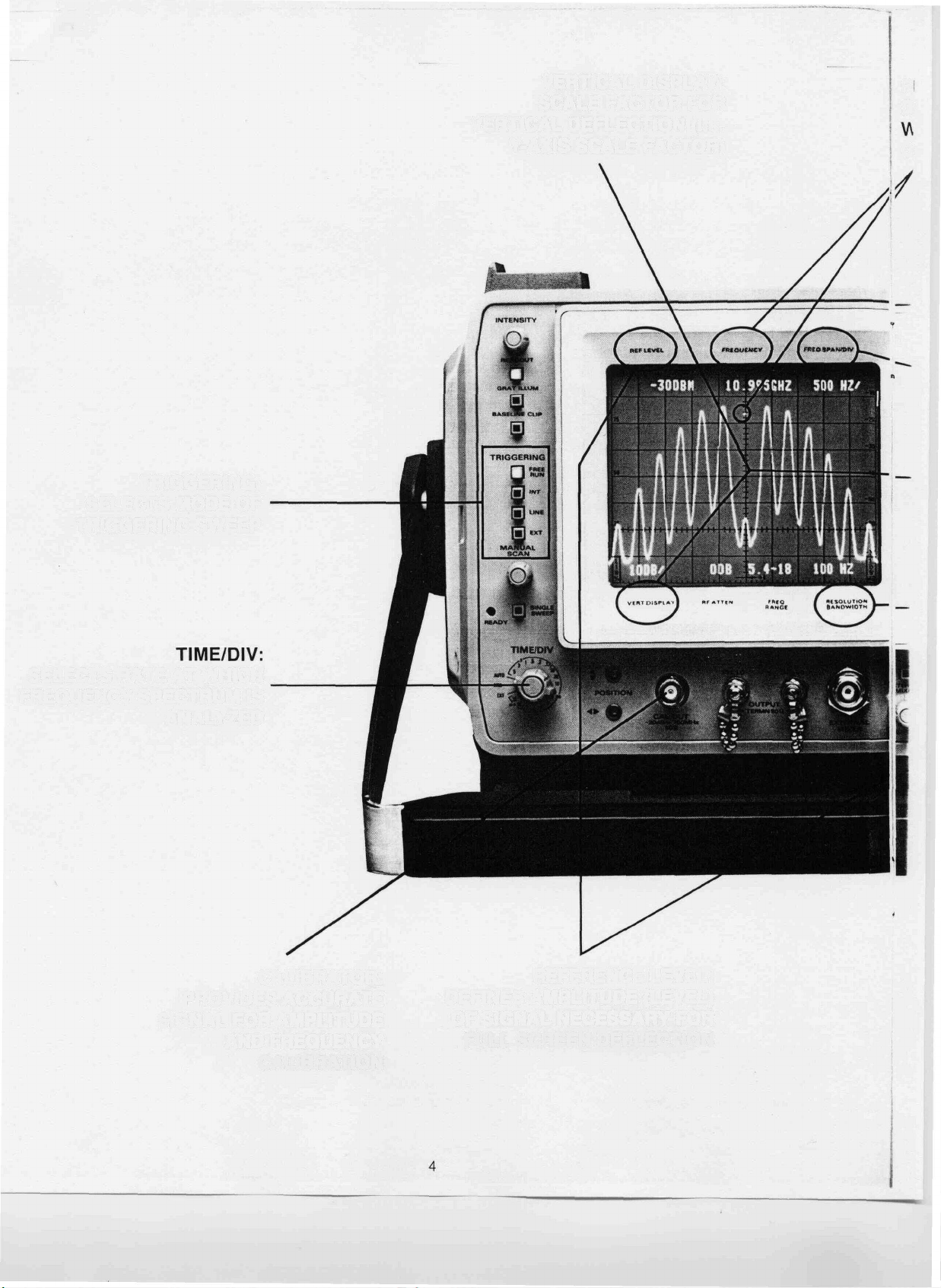
TRIGGERING:

SELECTS MODE OF

TRIGGERING SWEEP

VERTICAL DISPLAY:

SCALE FACTOR FOR

VERTICAL DEFLECTION (i.e.

Y-AXIS SCALE FACTOR)

F D

TIME/DIV:

SELECTS RATE AT WHICH

FREQUENCY SPECTRUM IS

ANALYZED

PROVIDES ACCURATE

SIGNAL FOR AMPLITUDE

AND FREQUENCY

CALIBRATOR:

CALIBRATION

REFERENCE LEVEL:

DEFINES AMPLITUDE (LEVEL)

OF SIGNAL NECESSARY FOR

FULL SCREEN DEFLECTION

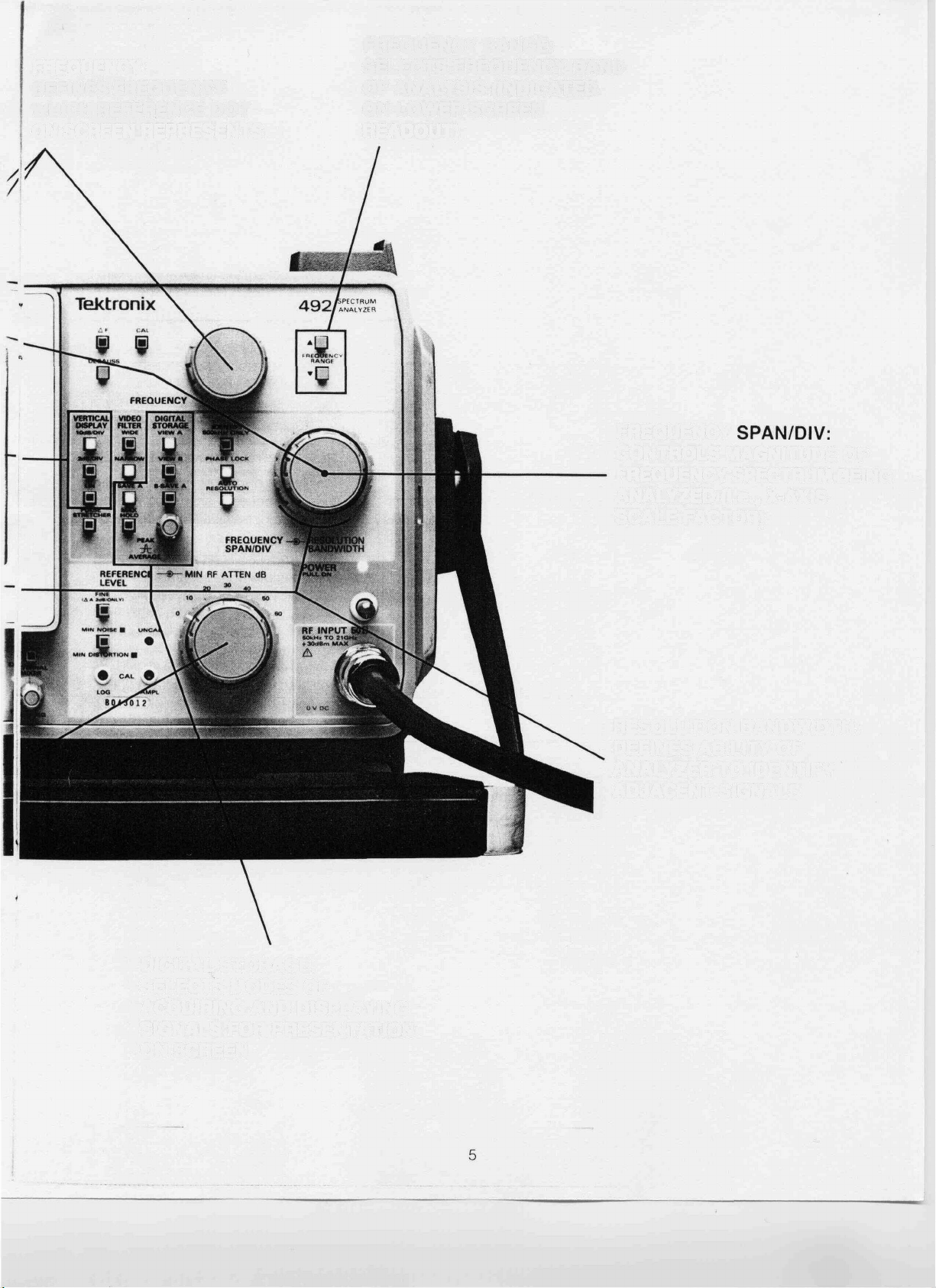
FREQUENCY:

DEFINES FREQUENCY

WHICH REFERENCE DOT ON SCREEN REPRESENTS

FREQUENCY RANGE:

SELECTS FREQUENCY BAND

OF ANALYSIS (INDICATED

ON LOWER SCREEN

READOUT)

FREQUENCY

SPAN/DIV:

CONTROLS MAGNITUDE OF

FREQUENCY SPECTRUM BEING

ANALYZED (i.e., X-AXIS

SCALE FACTOR)

RESOLUTION BANDWIDTH:

DEFINES ABILITY OF

ANALYZER TO IDENTIFY ADJACENT SIGNALS

DIGITAL STORAGE:

SELECTS MODES OF

ACQUIRING AND DISPLAYING SIGNALS FOR PRESENTATION

ON SCREEN

the input and a 1 st mixer that works

best with

-30

dBm, we need 53 dB

of attenuation for optimum operation

[ + 23 dBm (input) - 53 dB (attenua-

tion)

= -30 dBm

level)].

If the analyzer is tuned to

shift the larger signals off screen,

the RF attenuation still cannot be

removed to shift the

nal up on screen for better viewing,

(1st

mixer signal

-50

dBm sig-

because the input circuitry is still being exposed to the two larger signals. However, IF gain may be

added to increase the displayed

level of the smaller signal.

Unlike an oscilloscope, a Spectrum

Analyzer is ordinarily susceptible to

damage from dc voltages. This is extremely important to remember.

If a dc voltage can be applied to an

analyzer, it will usually be indicated

on the front panel near the input

connector. If dc voltage is a possi-

bility, always use an external Block-

ing Capacitor. Suitable blocking capacitors with good VSWR are

available from several vendors.

Frequency

Frequency Control

The Frequency control is the second

of the three main controls. This control identifies the frequency of a particular point on the display. Customarily, this is the center of the screen. In some modes of operation, however,

it could be some other point on the

screen. On many analyzers, there is

a dot or other indication on the dis-

play that indicates the point on

screen that represents the spec-

ified frequency.

Span Control

The Span control or Span/div control is the third of the three main controls. With this control, the width of the fre-

quency spectrum being analyzed

can be varied. When referred to as Span/div, it indicates "X" therefore, a 10 division screen would

be sweeping across a frequency

spectrum of

10x"X"

Hz/division;

Hz. (An ana-

lyzer that defines the Span control as just "span" will sweep that many

"Hz" across the screen.) As an ex-

ample, a span of 1

MHz/div,

would

sweep across a frequency spectrum

of 10 MHz. Just exactly which

MHz would depend on the Fre-

quency control. If the Frequency

control was set for

the analyzer would sweep from 95

MHz

to 105

MHz

100

(see

MHz, then

Fig.

5).

In Fig. 5, note that the large signal

100

MHz in frequency and has a

level of

-17

dBm. The smaller sig-

nals are at 98 MHz and 102 MHz at a level of -62 dBm. Since the smaller signals are symmetrical about the center signal, they could be the mod-

ulation of the carrier at

100

MHz. In

that case, the above example would

be referred to as a "signal" or "car-

rier" at 100 MHz with 2 MHz side-

bands down 45 dB from the carrier

(or

-45

dBc). (The term dBc means

below the carrier.)

Figure 5. With Frequency control set at 100

MHz and a Span of 1 MHz/div,

the displayed spectrum extends

from 95 MHz to 105 MHz.

The Span control has two settings

that are not calibrated in hertz. Turn this control clockwise to eventually reach a position of maximum (MAX) span. In this position, the analyzer sweeps across its maximum frequency spectrum for the band of frequencies selected. In a "band" that extends from 0 Hz to

1800

MHz,

the analyzer sweeps the frequency

spectrum from 0 Hz to

to look for signals when in MAX span. Although the analyzer is only

specified from 50 kHz to

a certain amount of oversweep is common. Turn the Span control

counterclockwise, and the spans get

smaller and smaller in frequency until the "zero" span position is reached. In this position, the analyzer no longer

1800

MHz

MHz,

sweeps across a frequency spectrum, but behaves like a superheterodyne receiver. The analyzer now basically works like a typical oscilloscope where the display indicates the

modulation of any signal at the fre-

quency selected by the Frequency control.

Resolution Bandwidth (RBW)

Ideally, the display or graph of amplitude vs. frequency should be vertical lines of minimum width to allow sig-

nals of very close frequency spacing

to be individually discernible as

shown in Fig. 6. Note the pair of

sidebands located very close to the

carrier. If a wide pen had been used

to draw the figure, as in Fig. 7, the

sidebands might have been over-

looked as denoted by the slight

width change near the bottom of the

carrier. Resolution Bandwidth (RBW) performs much the same function as varying the width of the pen when

plotting the display on the screen.

As the frequency spectrum being

displayed on screen varies as a function of the span/div, the width of the

"pen" that is calibrated in hertz must

also change. If an extremely narrow

"pen" is used with an extremely

wide frequency span, signals will

appear very narrow and may be overlooked.

Most modern Spectrum Analyzers

through the use of microprocessors

have the capability to select the optimum bandwidth (resolution bandwidth) depending on the span/div and time/div selected. There will be times, however, when manual con-

trol of this function will be desired.

Figure 6. Spectral graph drawn with fine tip

pen clearly showing closely

spaced signals.

Figure 7. Spectral graph drawn with broad

tip pen masking closely spaced

signals.

Resolution Bandwidth is a functional control that selects one of several bandpass filters physically located

in the instrument's Intermediate Fre-

quency (IF) chain. It is defined in the term Hertz (Hz) and is a measure of

the width of the filter either 3 dB or 6 dB down from its peak, depending

on analyzer manufacturer. The shape of the signals being traced out on screen are, in reality, a combination of the shape of the Resolution Bandwidth filter, and the signal, not just the shape of the signal being analyzed.

The limitations imposed on an ana-

lyzer by the Resolution Bandwidth

filter are significant. Sweep speed

(the rate the analyzer sweeps through the frequencies present) must be slow

enough to allow the filters to reach

peak amplitude or an inaccurate

signal amplitude will result. When

analyzing pulse type signals such

as radar, Resolution Bandwidth is

very important or erroneous results

will be obtained. This application will

be covered in more detail in the

Applications section.

Unless a special requirement dictates a specific Resolution Bandwidth, the Resolution Bandwidth selected should be somewhat greater than

1/50

the span/div. Figs. 8 and 9 show the two extremes of useful Resolution Band-

width for a particular span. In each

case, the signal being displayed is the same, with only the Resolution Bandwidth of the analyzer changing

between the two figures. Fig. 8 is

displayed with an extremely wide

RBW for the span/div selected. Fig. 9

has a more optimum RBW selected, and we can now see sidebands on

the signal that were not visible in

Fig. 8. If the bandwidth continued

to narrow, the sweep speed of the

analyzer would have to slow down

to allow the signal to trace the cor-

rect amplitude through the filter, and

the display would be less viewable.

Figure 8. 1 MHz RBW. Wider Than

Figure 9. 100 kHz RBW. Optimum

Optimum Bandwidth

Bandwidth Showing Signals Masked By Filter Skirts in Figure 8.

Another characteristic not yet men-

tioned, which works in our favor, is

that as the RBW is decreased, the

noise floor of the analyzer goes down. (The term noise floor refers to the baseline or lowest horizontal part of

the trace. Because of its appearance, this part of the signal is sometimes

referred to as the decade decrease in RBW (e.g. from

100

kHz to

of the analyzer decreases by

This is extremely important when looking for very small signals.

Figure

is a composite of two

RBW's that show a signal which

"grass".)

kHz), the noise floor

For each

dB.

was initially buried in the noise. The only parameter changed is the RBW,

which in effect, pushed the noise of the analyzer below the level of the

signal's sidebands.

Figure 10. Composite photograph illustrating

sidebands obscured by noise in wider resolution bandwidth.

Secondary Controls

Sweep Time

Like Resolution Bandwidth, most

newer analyzers have an Auto posi-

tion in which a microprocessor selects

the optimum sweep speed, depending on other parameters. When analyzing a frequency spectrum, this

control determines the rate at which

the analyzer sweeps through the determined spectrum. If the spectrum is swept too fast, the RBW filters may ring or fail to reach full amplitude. If

swept too slow, there are no disad-

vantages, unless the analyzer does

not have "digital storage" or some form of waveform storage. Without

storage, by the time an extremely

slow sweep is

tor could have forgotten the content

of the original spectrum.

complete,

the opera-

When the analyzer Span/div control

is set for Zero Span, the Sweep control functions like an oscilloscope's time control. As previously described, the display is a time domain presentation of the modulation at the center frequency selected when in Zero Span.

Video Filter (sometimes referred to as a Noise Averaging Filter)

This filter is used primarily as a smoothing filter to remove or smooth out the short duration noise spikes at

the bottom of the display. When the

analyzer is in Auto sweep speed,

note that the sweep rate decreases when a Video Filter is turned on. In most analyzers there are usually

several Video Filters to choose from.

Care must be taken, much like selecting the Resolution Bandwidth

filter. When analyzing a signal such as

pulse radar or if the Resolution Band-

width is very narrow for the span (i.e.,

narrow signals displayed on screen), the Video Filter should not be selected, as this will not allow the

amplitude of the analyzed signals to reach full amplitude due to its

video bandwidth limiting property

(i.e., a low-pass filter).

Digital Storage

In many older Spectrum Analyzers, a storage oscilloscope was used as the display. This was necessary

because of the slow sweep speeds

required to maintain amplitude cali-

bration. With the advances in digital

hardware, it is now possible to divide the screen into small horizontal segments and digitize the amplitude as the analyzer sweeps through each

segment and store the data in RAM (random access memory). This data

can then be accessed, converted to

analog signals, and sequentially dis-

played on the screen in the proper

horizontal sequence at slightly above

flicker rate.

This procedure of digitizing a signal occurs after the signal has been processed by the Resolution Bandwidth

(RBW)

circuitry, the Logarithmic (log)

circuitry, and Video Filter circuitry. It

usually occurs just prior to being

amplified for the crt.

Once the data is stored in RAM, we

usually have an option as to the

method of display. If we desire to

"SAVE" a particular waveform (e.g.,

"A" waveform), we can select the

"SAVE A" function and the "A

memory" within the analyzer will be frozen and not updated. The B waveform in memory will continue to be updated with each sweep of the

analyzer; thus we would view separate traces on the screen. If the

"SAVED" trace was not needed for

immediate viewing, the "VIEW A"

function could be disabled and the

"A memory" would not be displayed

on the screen; but, its data would

still be available for future reference.

If the "VIEW B" function is simultaneously disabled, the display portion of Digital Storage is disengaged and

the sweeping signal of the analyzer

will be displayed, with the refresh rate determined by the control.

The

"B-SAVE

A" control is used to

Time/Div

display the difference between two

waveforms. As the name implies, it subtracts the SAVED A waveform from the active B waveform. This function is most useful when the analyzer is used with the Tracking

Generator. (This application will be

discussed in the Applications sec-

tion dealing with the Tracking Generator.)

The "MAX HOLD" function is used to capture the maximum Y deflection (amplitude) for any X axis position (frequency), regardless of how many sweeps must be made to capture these extremes. This is accomplished by the digital storage digitizing new amplitude data for a particular point

on screen, then checking the amp-

litude in memory for that specific

memory location and saving the

larger of the two. The usefulness of "MAX HOLD" is in capturing a fre-

quency spectrum where a signal

randomly appears, then disappears. Once the signal has been analyzed

and stored, the digital storage will continue to display the signal, re-

gardless of whether or not it reap-

pears on succeeding sweeps. A different application might be to

monitor an FM'ing or drifting signal

and note the frequency excursions.

This can be accomplished by se-

lecting the desired frequency carrier and enabling the "MAX HOLD" function. On each succeeding sweep,

the analyzer will analyze the carrier

at its precise frequency at the mo-

ment of analysis and save this value in memory. With repetitive sweeps, the maximum excursions will be filled

and viewable for analysis. It is im-

portant to check the drift specifications of the analyzer to ensure the

analyzer is more stable than the sig-

nal to be checked. The

Peak/Average

determine data processing prior to

loading the digitized information in RAM for a particular horizontal point

on the screen. For each horizontal

point on the screen (of which there

are 1000) the digitizer may digitize

from 2 to ing on the sweep speed) to represent the Y value to be stored for a particular horizontal point. If the amplitude of the signal at this horizontal point is above the cursor, the storage will select the maximum

10,000

cursor is used to

samples (depend-

value digitized and load this num-

ber in memory; thus, the term "Peak Detect". When the amplitude of the signal at this horizontal point is located below the cursor, the digital

storage will take the mathematical

average of the digitized numbers and load this number in memory;

thus,

the

term "Average Detect".

The necessity for having a

"Peak/

Average" function is to ensure that

the maximum value of a narrow

pulse can be stored to represent the

maximum amplitude of that pulse,

and "noise" or "grass" can be

averaged before storing in RAM to

offer the maximum possible signal-

to-noise ratio.

Frequency Range

This

function operates much

a "Band Select" switch on a shortwave receiver. Each succeeding selection of either the "up" or "down" control

will

place the instrument in a higher or lower frequency band of operation.

Phase Lock

An analyzer usually has two or more

internal

oscillators,

one or more of

which will be swept (or moved) as the analyzer

sweeping through a

frequency spectrum. When in wide

spans,

such as

100

kHz/div

or greater, a slight amount of drift in one of the

internal

oscillators is usually not no-

ticeable.

However,

as the span

reduced to several kHz/div or less,

the instability of the internal oscillators

becomes apparent. The screen indi-

cation

of an apparently drifting

signal, when the real problem is a

drifting oscillator within the analyzer.

Therefore, when an analyzer is op-

erating in the narrower spans, the

oscillator causing the drift problem

typically phase locked to a stable

reference to prevent the drift. In

wider

spans/div,

this

oscillator is typically being swept; therefore, it cannot be locked at all times. When

the phase lock circuitry is operating, a front-panel indicator will typically

inform the operator.

This

indication

requires no action on the user's part

and will usually not affect the meas-

urement

an adverse way.

Preselector

A Preselector is a filter located just slightly behind the input connector.

The function of the filter

to select or

allow only a narrow band of frequen-

cies to pass

into

the analyzer. It

sweeping filter that tracks the fre-

quency the analyzer is tuned to at

any particular point in

tion

performs

time.

The func-

to inhibit harmonic mixing within the first converter. By eliminating the harmonic conversions, unwanted mixing products do not appear as signals in the spectrum. In addition, any large signals (up to

+ 30

dBM)

present on the input but

out of the frequency range being

analyzed are prohibited from reach-

ing the input mixer, thus eliminating

the need to use attenuation to pro-

tect the input mixer from burnout.

The preselector

almost transparent

to the user, except that it needs to

be "peaked" occasionally. This is

usually accomplished with a front-

panel control. The "Peaking Control"

allows the user to offset the tracking filter slightly forward or backward

with

respect to the frequency the

analyzer is tuned

(i.e.,

to be cen-

tered around the tuned frequency).

If the filter is mis-peaked and is

completely offset from the tuned

frequency, the analyzer will indicate

a complete lack of signals in the

preselected bands. Preselection

occurs only

(1.7

— 21 GHz)

bands 2 through 5

the 490 Series of

Spectrum Analyzers.

Applications

Amplitude

(AM) Notes

An Amplitude Modulated signal, when viewed in the (as with an oscilloscope), might ap-

pear as

we can determine the frequency of the carrier (fc) and the frequency of the modulation

percent of modulation can be cal-

culated from the equation:

%Mod

Figure

nal being displayed in the frequency

domain on a spectrum analyzer.

Modulation

time

domain

Fig.

11.

From

this

photo,

(fm).

In addition, the

represents the same sig-

x100.

From this display, the frequency

of the carrier (fc) and the frequency

of the modulation (fm) can also be

determined. The percent of

modula-

tion can also be determined by not-

ing the difference

amplitude

(12

dB) between fc and fm and using

the table in

Figure

Figure 12. AM Modulation

Modulations

Figure

Fig.

13.

11.

AM Modulation (50%) in time

domain.

•REOUENCV

SPAWDIV

frequency

domain.

200

13.

Chart of dB vs.

(dB down from Carrier)

x 10

°/o

of Modulation.

Figures 11 and 12 were prepared under controlled test conditions. In normal operation, the modulation will not be a pure sine wave, but will be a composite of multiple sine

waves, and their frequencies cannot

be determined in the time domain. However, the Spectrum Analyzer will accurately display all frequencies present.

A suppressed carrier system would

be displayed on the analyzer as in Fig.

14.

The typical measurements

to be made in this system would be carrier suppression. The measurement is the difference in carrier am-

plitude between when the carrier is

turned on and when it is turned off.

Fig.

indicates the carrier is sup-

pressed by 40 dB.

VARIABLE FREQUENCY OSCILLATOR

Figure

15.

Test setup for sweeping audio flatness.

system described, and Fig.

is a

photo of such a sweep.

From Fig.

flatness is

we can see the system

1.3

dB (which in reality may

be a type of emphasis placed on

the audio), and the system 3 dB

bandwidth is in excess of 8 kHz.

Both lower and upper sideband envelopes should be symmetrical. If the transmitter were seriously mistuned or was working into a poor antenna match, the Spectrum Analyzer would show how each side-

band was individually affected.

modulator should be driven to a specified percent of modulation and the Spectrum Analyzer should be checked for the presence of only the signal that is put into the modu-

lator. If harmonic distortion is occur-

ring, additional products will appear

on the screen at multiples of the modulating frequency. Fig. 17

shows the result of a modulator be-

ing driven with a 5 kHz test signal.

Harmonic distortion will show up as signals at

kHz,

kHz, 20 kHz,

etc. from the carrier. The Total Har-

monic Distortion (THD) can be de-

termined by noting the amplitude

difference between the modulation signal and its harmonic products.

-igure

14.

Suppressed Carrier System

Similarly, if the lower sideband was suppressed as well, we could determine the amount of this suppression by noting the difference in amplitude between the upper and lower sideband.

Another type of measurement that

could be made on an AM system would be to check system flatness by sweeping the audio input with an

audio generator of known or verified flatness. The RF carrier could then

be monitored in a narrow span/div and a deflection (scale) factor of 2

dB/div.

By using the MAX HOLD

function, we could construct a waveform to indicate the flatness of the total system. This waveform would also indicate any "emphasis" placed

the audio. Figure

shows the

Figure

16.

Audio flatness of AM system as

measured at RF frequency.

Distortion

Distortion is the result of electronic circuits operating in a non-linear

mode. Two of the most common

methods of checking for distortion

involve driving the equipment with

known signals and monitoring the

equipment output for signals other than those present at the input.

(Harmonic Distortion) A typical

Harmonic Distortion measurement

would be set up as in Fig.

with

the variable frequency oscillator set at some specified frequency. The

Figure 17. Harmonic Distortion at 10 kHz,

kHz, and 20 kHz from Carrier.

The sum of all the harmonic products

must be used to determine the per-

cent of harmonic distortion. The Total

Harmonic Distortion (THD) can be

determined by noting at what level below the fundamental each har-

monic lies, and determining the

percent ratio for each harmonic

from Fig. 18 and substituting in the

following equation. This equation is

only accurate if the upper and lower

harmonic pairs are within one or two

dB of each other.

THD(%)=

V(2nd

Harmonic

+ (3rd Harmonic

+ (4th Harmonic +

etc.

%)2

From Fig. 17, the THD is

V0.03252 + 0.0122 + 0.00182

= 0.035 = 3.5%

When making this measurement, it is important to be sure the modulating signal from the audio oscillator is free from any harmonics. To do this, check the signal source with a

Spectrum Analyzer.

10 20 30 40 50 60 70

Figure 18. dB below Fundamental to '

dB BELOW FUNDAMENTAL

Distortion.

(Intermodulation Distortion) An

additional measurement common

to amplifiers or transmitters is the

Two Tone Intermodulation Distortion

(IM)

test. This test is similar to the Harmonic Distortion check, except it requires an additional audio sig-

nal generator. The two audio gen-

erators are combined, and the result

is applied to the modulator. The method of combining the two sig-

nals is very important, as mixing the

two sources with each other can create unwanted products. Com-

bining should occur in a directional

bridge. A

"T"

connection or com-

biner can be used, provided each generator is sufficiently padded. A

Spectrum Analyzer should be used to check the output of the directional bridge or combiner for any signals other than those applied prior to

modulating the transmitter. The fre-

quency of the modulating signals

depend on the type of test to be performed and the type of equipment being checked. Our example uses a 4 kHz

(f-|)

and 5 kHz

(f2)

sig-

For more information on these and

other tests on AM systems, see

Tektronix, Inc. Application Notes

AX-3266, "AM BROADCAST MEA-

SUREMENTS USING THE SPEC-

TRUM ANALYZER", and 26W-4889,

"NO LOOSE ENDS — REVISED.

THE TEKTRONIX PROOF OF PERFORMANCE PROGRAM FOR

CATV."

nal. There are multiple IM products created, of which the first one is called the second order

product, which will occur around the carrier at

f1 +f2,

f-i

-f2 and/or

f2-f1 (9 kHz

and 1 kHz from the carrier). The third

order

products will occur at

2f-|

+f2,

2f-|

-f2,

2f2 +

f1,

and/or

2f2-f1 (13 kHz, 3 kHz,

6 kHz, from the carrier.) Fig.

kHz, and

shows a typical response and identifies the various 2nd and 3rd order

products.

Tracking Generator — TG

(with Spectrum Analyzer

for Swept Measurements)

A Tracking Generator (TG), when

used in conjunction with a Spectrum

Analyzer (SA), allows such items as filters, amplifiers, couplers, etc. to be observed with respect to frequency

(i.e., Frequency Response). This is

performed by connecting the output

of the TG (TG output frequency is

synchronized to frequency being

analyzed by Analyzer at any point

in time i.e., "Tracking Generator") to

the input of the device being tested,

and monitoring the output of the

device with the SA (as shown in

Fig. 20). This type of measurement

is known as an

S12

measurement, since the phase shift

of the signal through the device is not displayed.

Figure

19.

Distortion showing input signals

and both Harmonic Distortion

(2f,,

2f2,

etc.) and IM products

(second

order:

f2-'1,

(3rd

order:

2f1-f2,2f2-fl,

2f, + f2,

2f2 +

f1),

order products.

TRACKING

GENERATOR

Figure 20. Spectrum Analyzer (SA) and Tracking Generator (TG) Test Setup.

\\ + f2),

plus higher

INTERFACE

The response displayed on the

screen of the analyzer will be a

combination of the unflatness of the TG and the response of the device

being tested. The unflatness of the

SPECTRUM ANALYZER

CABLES

DEVICE

UNDER TEST

magnitude only

TG/SA can be removed by using the

"B-Save

A" function of the SA. First,

connect the TG to the SA and save the flatness (or

TG/SA

unfiatness)

of the

the A memory by using the SA "Save" function, and using the "Vert Display" mode that will be

used

the measurement. Then, connect the TG to the device being tested and monitor the device

with

the analyzer. Once a sweep has

been made, the analyzer display

will

indicate the system response.

By activating B-Save A, the saved un-

fiatness of the TG

will

be subtracted

from the response of the system, and the corrected display will indicate the corrected frequency re-

sponse of the device being tested.

The photographs that follow indicate the typical responses of the systems shown.

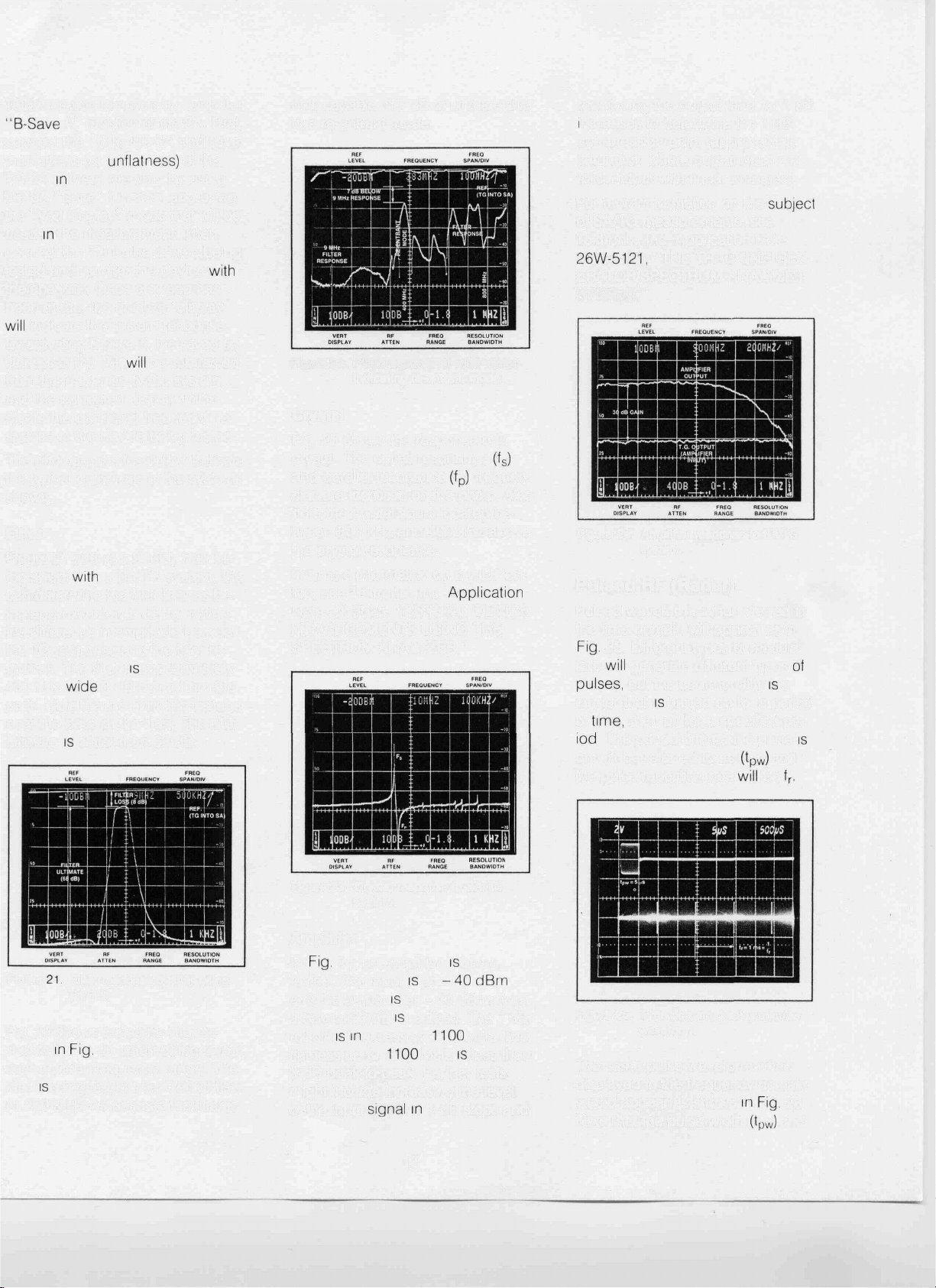
Filter

Figure 21 shows a 9 MHz filter being swept

with

a SA/TG system. We

can determine the filter loss as be-

ing approximately 8 dB by noting

the difference in amplitude between

the TG response and the filter re-

sponse. The filter 400 kHz

wide

approximately

3 dB down from the

peak. Note the unsymmetrical shape

near the base of the filter. The filter

ultimate

better than 68 dB.

only capable of 7 dB of ultimate due

to a re-entrant mode.

Figure 22. Filter response at wide sweep

indicating re-entrant mode.

Crystal

Fig. 23 shows the response of a

crystal. The series resonance and parallel resonance

(fp)

frequen-

(fs)

cies are identified on the photo. Also

note the crystal spurs located be-

tween 300 kHz and 400 kHz above

the crystal resonance.

For more information on crystal test-

ing, see Tektronix, Inc.

Application

Note AX-3525, "CRYSTAL DEVICE

MEASUREMENTS USING THE SPECTRUM ANALYZER."

monitoring the output level for 1 dB

ncreases to determine the 1 dB

compression point (approaching saturation where output does not follow input with linear changes).

For more information on the

subject

of SA/TG measurements, see

Tektronix, Inc. Application Note

26W-5121,

ERATOR/SPECTRUM ANALYZER

SYSTEM."

Figure 24. Amplifier response to SA/TG

"THE TRACKING GEN-

system.

Pulsed RF (Radar)

Pulsed waveforms when viewed in

the time domain will appear as in

Fig.

25. Different types of modula-

tors

will

generate different types

pulses,

but the commonality

carrier that of

time,

iod

The period of time the pulse

on will be referred to as

the pulse repetition rate

turned on for a period

then off for a specified per-

(tpw)

will

and

fr.

Figure

21.

Filter response of filter using

SA/TG.

Fig. 22 shows the same filter as

shown

Fig.

21 when being swept

over a wider frequency range. The

filter

being tested from 0-900 MHz.

At 350 MHz we can see the filter is

RESOLUTION

Figure 23. Crystal response to SA/TG

system.

Amplifier

Fig.

24, an amplifier tested. The input and the output

a gam of 30 dB

roll-off

is m excess of

flatness up to

1100

being

-40

dBm

at - 10 dBm, thus,

realized. The 3 dB

1100

MHz. The

MHz

less than 3 dB peak-to-peak. Further tests might include increasing the level of the input

signal

1 dB steps and

Figure 25. Time domain display of pulse

waveform.

The same pulse waveform when displayed in the frequency domain would appear as shown

Note that the pulse width

(tpw)

Fig.

26.

and

the repetition rate

(fr)

can be deter-

mined from the spectral display.

Figure 26. Frequency domain display of

pulse waveform.

sweep time/div 10 ms

*r= #pulses/div =H'0~

1______1

- lobe width ~ 200 kHz ~ 5 ^

In the introduction, we learned that

all waveforms can be described as

a combination of various sinusoidal waveforms of differing amplitudes.

The pulses in Fig. 25 are likewise

composed of an infinite number of

discrete sinusoidal frequencies of differing amplitudes. Since there are

an infinite number of signals, we are

primarily interested in the envelope

of the amplitude of the signals. In

our example, this is described by a

sin x

display shown in Fig. 27. We can see that the amplitudes in Fig. 26

lie within the area described by Fig.

27. The big question is "Why do we

see discrete signals in Fig. 26 if the

waveform is composed of an infi-

nite series of frequencies?"

Figure 27. Envelope of pulsed signal

sin x

—— envelope I

The answer lies in the fact that swept frequency analyzers only analyze a specific frequency at a specific time as the beam traces across the screen. Each time a pulse is generated, the analyzer will analyze the amplitude

of the frequency component at the

frequency being analyzed at that instant. If the pulse repetition period

(tr)

of the pulse was 1 ms and the analyzer was sweeping through the frequency spectrum at 1 ms/div, we would see one spectral

we slowed the sweep speed to

line/div.

100

ms/div, we would obtain 100 spectral

lines/div,

which would clearly show

the envelope display of Fig. 27. We

need to remember that although we

are varying the sweep speed, we

are not changing the span of fre-

quencies being analyzed, just the rate at which we are analyzing them. To compute the repetition rate from

Fig. 26, determine the number of

divisions/spectral line and multiply

by the sweep speed/division.

To display an optimum waveform of pulsed RF, the Resolution Bandwidth (RBW) should be selected narrow enough to display each spectral

line. As the RBW is narrowed, the

amount of energy from the pulse reaching the detector within the analyzer is reduced and the display will

indicate a lower level signal than is

actually present. The optimum

Resolution Bandwidth (RBW) is ap-

proximately

tpwxRBW

0.1/pulse

width

(tpw)

equal-to-or-less-than

0.1.

Figure 28 shows the optimum RBW as a function of pulse width, and Fig. 29 shows the approximate sensitivity

loss or signal amplitude loss as a

function of the product of

tpw x RBW

(pulsewidth x Resolution Bandwidth).

Note that the type of Resolution Bandwidth Filter in the analyzer

will vary the amount of loss between

Pulsed RF and a CW signal of equal amplitude. 490 Series filters are of the rectangular response. Since there is a signal loss through an analyzer

due to RBW limitations, it is important

to remember that the front end of the

analyzer is being driven harder than

the signals on the screen indicate.

Care should be taken not to overdrive the input mixer.

600 400

*-_

(£>

CO/-

CVJ T (D

PULSE

Figure 28. Resolution bandwidth setting

for pulsed RF computed from

[tpw]xRBW = 0.1

.001

PULSEWIDTH-BANDWIDTH

Figure 29. Sensitivity loss of pulsed

signals vs CW.

COO O O

WIDTH

(!,„)-

pi"

.01 .1 1

PRODUCT

(t^xRBW)

For best results when analyzing

pulsed RF, Digital Storage should be disabled until the optimum combination of sweep speed, span/div,

RBW and Reference Level have been achieved. Once the desired waveform has been acquired, the

storage can be activated with the

Peak/Average cursor placed at the bottom of the screen. The Auto Sweep speed (time/div) and Auto

RBW should not be used, as the

algorithm used to compute the opti-

mum setting is not valid for pulsed

RF.

Typical observations of an RF spectrum

would

be the following:

1. For a rectangular pulse, the 1st

sidelobe

13.3 dB below the (see

should be approximately

main

Fig.

26).

lobe

2. If the nulls are not well defined,

the

pulsewidth

(see

Fig.

27).

(tpw)

FM'ing

3. Poor carrier on/off ratio shows up as a response buried under

the

main

lobe (see

4. If the carrier

Fig.

30).

FM'ing, the lobes

could be unsymmetrical (see

Fig.

31).

Figure 30. Note void in main lobe and

pulse extension on top of main lobe caused by poor carrier on/off ratio.

For further information on

this

sub-

ject, see Tektronix, Inc. Application

Notes AX-4217, "PULSED RF

SPECTRUM ANALYSIS" and

AX-3259, "NOISE MEASUREMENTS

USING THE SPECTRUM ANALYZER

— PART TWO; IMPULSE NOISE."

Noise Measurements

Noise measurements are often

made as carrier-to-noise (C/N) measurements, oscillator spectral purity,

white noise level, etc. The noise referred to signal or "grass" of a spectrum dis-

play. The unit of measure when deal-

ing with random noise is usually

dBm/Hz or Watts/Hz. The noise band-

width must always be specified, be-

cause each decade of change

noise bandwidth will vary the measurement by 10 dB. Random Noise implies the noise is being analyzed through an idealized square-shaped filter. Since most filters are not of the

idealized square shape, a correction factor may have to be generated to

convert from the Spectrum Analy-

zer's Resolution Bandwidth (RBW)

to the effective Noise Bandwidth of

each filter. This correction is ex-

the level of the baseline

plained

Tektronix, Inc. Application

Note AX-3260 "NOISE MEASUREMENTS USING THE SPECTRUM

ANALYZER - PART ONE: RANDOM

NOISE." If

this

correction

not

made for the RBW used, errors of

up to 2 dB can occur

the meas-

urement. Another source of error when mak-

ing noise measurements occurs in

the detector and logarithmic circuitry.

These two errors cause the measured noise to appear lower in level than the actual noise by the following

factors:

LIN

display mode: 1.13 dB

LOG display mode: 2.5 dB

An additional source of error involves dealing with very low level signals or

in this case, system noise located close to the noise floor of the analyzer. To test for the

analyzer's

noise floor, disconnect the input and note the amplitude of the noise. When a signal or system noise

within

dB of the analyzer noise

located

floor, the amplitude of the measured

signal or system noise cated as being higher than

by a factor as determined

will

be indi-

really

Fig.

32.

Figure

31.

FM'ing carrier.

WARNING

Radar applications require relatively large amounts of power for proper

operation. Signal access points on

radar systems often have large sig-

nal levels that can be lethal to both people and Spectrum Analyzers. The input circuitry of Spectrum Analyzers is fragile. Use caution and plenty of external attenuators when observing unknown signals.

INDICATED SIGNAL

AMPLITUDE ABOVE

ACTUAL SIGNAL

AMPLITUDE

2dB

Figure 32. Amplitude correction for signals located within 10 dB (low level signals) of analyzer

noise floor.

4dB

DIFFERENCE BETWEEN ANALYZER NOISE FLOOR

AND LOW AMPLITUDE SIGNALS (OR SYSTEM NOISE) IN dB

6dB

8dB

In our example of Fig. 33, the difference of analyzer noise floor to system noise floor is 5 dB. From

Fig. 32, a correction factor of

1.7

dB must be subtracted from the indicated system noise amplitude to obtain the true noise level. (Remem-

ber that two signals of the same am-

plitude will indicate 3 dB more power than the amplitude of either of the signals. Thus, a signal measured 3 dB above the noise is actually at the same amplitude as the noise.)

Figure 33. Carrier-to-noise ratio measure-

ment including correction for

low amplitude system noise.

A system will quite often have a noise specification of a noise bandwidth in other than a common Spec-

trum Analyzer RBW. To get from

one bandwidth to another bandwidth, the following formula can be used.

C/N at Specified Bandwidth (dB) = C/N at Measured Bandwidth (dB)

Specified Bandwidth (Hz)

1f)

Measured Bandwidth (Hz)

Using Fig. 33 as an example, we

measured the carrier-to-noise ratio

of a system as being 65 dB in a 100 kHz RBW. The system specification requires the result to be a 4 MHz noise bandwidth.

C/N at 4

MHz

= 65 dB at

100

kHz

minn 4 MHz

-10'°g 100kHz

= 65

dB-16

RBW

dB = 49 dB at 4 MHz

ror and RBW/Noise Bandwidth cor-

rection factor and signal noise

floor/

analyzer noise floor correction factor.

Each analyzer's RBW/Noise band-

width correction factor must be

compiled per the previously men-

tioned Tektronix, Inc. Application

Note AX-3260. Let us assume a 1

dB error.

C/N at 4 MHz noise bandwidth = C/N at 4 MHz

RBW + signal noise

floor/

analyzer floor correction - RBW/noise

bandwidth correction factor - Log

Error

For our example, then

C/N at 4 MHz noise bandwidth =

49 dB at 4 MHz RBW

dB RBW/noise

bandwidth-2.5

+1.7

-1

(C/N of example = 47.2 dB at 4 MHz

noise bandwidth)

For more information on the subject of Noise, see Tektronix, Inc. Appli-

cation Notes AX-3260 "NOISE

MEASUREMENTS USING THE SPECTRUM ANALYZER — PART ONE: RANDOM NOISE", AX-3259, "NOISE MEASUREMENTS USING THE SPECTRUM ANALYZER —

PART

TWO: IMPULSE NOISE",

and 26W-4889, "NO LOOSE ENDS

- REVISED: THE TEKTRONIX PROOF OF PERFORMANCE PROGRAM FOR CAW."

INTERFACE

TRACKING

GENERATOR

CABLES

SOURCE REFLECTED

Antenna Sweeps (SWR)

Antenna sweeps are performed on antenna systems to determine if the antenna is "tuned" for the frequency at which it will transmit or receive.

An improperly tuned transmitting

antenna can cause much of the energy created by a transmitter to be reflected back into the transmit-

ter causing

Intermodulation

tion thus causing a loss of effective

power being radiated. A properly tuned antenna will have its characteristic impedance at the frequency

of intended use. The measurement

of a system standing wave ratio (SWR) can be made using a Spectrum Analyzer, Return Loss Bridge, and a Tracking Generator or Sweeper

capable of operating at the fre-

quency of antenna operation. From the SWR, you can determine the sys-

tem impedance at any frequency

over which the SWR was measured. SWR measurements are made using

the mentioned equipment and con-

nected as shown in Fig. 34. A Return

Loss Bridge designed for the characteristic impedance of the antenna

must be used.

SPECTRUM ANALYZER

RETURN LOSS

BRIDGE

LOAD

Distor-

The actual C/N at 4 MHz Noise

Bandwidth is then determined by

accounting for the analyzer's log er-

Figure 34. SWR test setup.

The system operates by the signal

source (Tracking Generator in

this

case) launching a signal at a specific frequency to the Return Loss Bridge

(Bridge)

The Bridge routes the sig-

nal to the antenna or system under

test, but not to the analyzer. If the

termination

looks

at the end of the

the system characteristic

line

impedance, all the energy is ab-

sorbed and nothing

the termination

reflected.

not at the charac-

teristic impedance, a portion of the energy

will

be reflected back to the

Bridge where

will

be routed to the Spectrum Analyzer and displayed on

screen.

As the sweeper or tracking generator sweeps across the frequency band lyzer

will

plot a graph of Return

selected,

the ana-

Level or Return Loss (in dB) vs. frequency.

System

calibration

requires terminat-

ing the antenna end of the cable

with

an "open" or "short" to reflect all the energy the analyzer

back,

and adjusting

with

a display at the top of the screen. Then, by terminating the antenna end of the cable into

the characteristic impedance, the

operator can determine the display level representing the characteristic impedance.

Fig.

35 shows a typical

display of an antenna trimmed or

tuned for operation at 135 MHz.

FREO

RESOLUTION

Figure 35 demonstrates a narrow

band antenna being swept from 35 MHz to 235 MHz. The antenna

showing a 40 dB "Return Loss" at

135 MHz. From

Fig.

36 we can de-

termine the antenna's SWR as being

1.02:1.

110

MHz, the SWR =

2.0:1

One of the limitations and problems

associated

is:

Most signal sources are only

with

the setup of

Fig.

capable of generating between 1

mW and 1 W of power. Therefore,

the analyzer

will

be set

with

very little RF attenuation. If another nearby transmitter broadcasts during the period the test excessive power could be

being conducted,

received

by the antenna being tested and damage the Spectrum Analyzer. If an amplifier

available to place

between the tracking generator and

the Bridge to boost the power (am-

plifier system

flatness), then

should

external

be checked for

attenuators can be placed between the Bridge and Spectrum Analyzer to reduce

the signal and protect the analyzer.

RETURN LOSS

.02 .05 .1 .2 .5 .7

i1!;

"--

H-4

—

T——

•

rr:

—

o_>*

••»'•'

-4-

1.05

ai:

r—

™

•^*s

_..

1.1 1.2 1.4 1.6 1.8 2.0 3.0 5.0 7.0 9.0

REFLECTION COEFFICIENT

SWR, P

ETURN

?S4,

1-10"

The Return Loss Bridge specification should be checked for power

handling

Extreme caution must be practiced when operating an analyzer near high power RF equipment. Excessive power applied to the input will damage a Spectrum Analyzer.

capability

WARNING

For more information on SWR

Measurements,

Application Notes

see Tektronix, Inc.

26W-5121,

TRACKING GENERATOR/SPEC-

TRUM ANALYZER SYSTEM" and

AX-3842, "TROUBLESHOOTING

TWO-WAY RADIOS WITH THE

SPECTRUM ANALYZER."

Other Application Notes of interest:

"EMI

MEASUREMENTS USING A

SPECTRUM ANALYZER" 26W-4971.

"EMI APPLICATIONS USING THE

SPECTRUM ANALYZER" AX-3406-1.

"DIGITAL RADIO MEASUREMENTS USING THE SPECTRUM ANALY-

ZER" AX-4457.

"FM

BROADCAST MEASURE-

MENTS USING THE SPECTRUM

ANALYZER" 26AX-3582-3.

LOS

*S«

...

/Return

S, R

SWR

EFL

•s-.

Loss dB

Loss

"" " /

dti

(

;OEFFICIEN

"~~^.

--—,

"THE

:::: ;:

•~-- — .

Figure

Return Loss of Narrow Band

Antenna with 40 dB Return

Loss

Figure 36. SWR, Return Loss, and Reflection Coefficient Chart.

Glossary

AMPLITUDE MODULATION (AM): The process, or the result of the process, whereby the amplitude of one electrical quantity (carrier frequency) is varied in accordance with some selected characteristic of a second quantity (modulating

frequency)

B-SAVE-A: A mode of display whereby a waveform which is stored in a digital memory is subtracted from a waveform stored in a second memory with the being displayed on screen.

BASELINE CLIPPER: A means of blanking the signal at the baseline portion of the display.

CALIBRATOR: A signal generator whose output is used for purposes of bration, normally either amplitude or frequency or both.

CARRIER: The wave (frequency) to which modulation CENTER FREQUENCY: That frequency which corresponds to the center of a fre-

quency span, (Hz).

COMB GENERATOR: A signal source which produces a frequency and multiple harmonics of the fundamental frequency. Signals are equally spaced at the fre-

applied.

quency of the fundamental.

DEGAUSS: To neutralize the residual magnetic polarity of an electronic device by

electric means.

DELTA F: A difference in frequency. A mode of operation of an analyzer where the

difference in frequency of two signals can be read out directly.

DIGITAL STORAGE: A means of storing the display in modern spectrum analyzers. Allows for flicker-free displays that may be held in memory. Also includes

capabilities such as digital averaging and storing maximum signal excursions.

DIPLEXER: A device capable of simultaneously directing one signal out and

receiving another signal on the same port. The received signal is then routed out in

a separate port.

DISTORTION: An undesired change in waveform caused by signal processing in

a non-linear device or system.

DYNAMIC RANGE: The maximum ratio of two signals simultaneously present at

the input which can be measured to a specified accuracy.

EXTERNAL MIXER: A device used to analyzer with RF frequencies. This mixer is external to the analyzer. Typically the

mixing

occurring within a waveguide. FILTER: A circuit for separating signals on the basis of their frequency. 1ST LO OUTPUT: A port on a spectrum analyzer where the

quency

made available for use outside the analyzer.

FLATNESS: The unwanted variation of the displayed amplitude over a specified

frequency span, expressed in

FREQUENCY BAND: A range of frequencies that can be covered without switching

(in

units of Hz).

FREQUENCY MODULATION (FM): The process, or the result of the process,

whereby the frequency of one electrical quantity (carrier frequency) is varied in

accordance with some selected characteristic of a second quantity (modulating

frequency). FREQUENCY RANGE: That range of frequencies over which the instrument per-

formance is specified (Hz to Hz). May refer to the range of frequencies available in

a particular band.

FREQUENCY SPAN: The magnitude of the frequency band displayed, expressed in hertz or hertz per division.

HARMONIC: A sinusoidal component of a periodic wave or quantity having a fre-

decibels

mix

the

1st

local oscillator of a spectrum

1st

local oscillator fre-

quency that is an integral multiple of the fundamental frequency.

HARMONIC (N) MIXING: The product of one signal combining with harmonics of a second signal. This method of mixing is used in spectrum analyzers to obtain coverage in higher frequency bands than would otherwise be possible with

mental conversions.

IDENTIFY CONTROL: A function which enables the user of an analyzer to

determine

cated or

IF (Intermediate Frequency): A frequency at which the input signal is shifted

internally for processing.

INTERCEPT POINT: The theoretical points at which the fundamental (driving) signals and the distortion products have equal amplitudes.

LINEAR DISPLAY: A display in which the vertical scale divisions are a linear function of the input signal voltage.

LOG DISPLAY: A display in which the vertical scale divisions are a logarithmic function of the input signal power.

MAX HOLD: A mode of acquisition for a digital storage system where the maximum amplitude achieved at every frequency being analyzed is retained and continuously displayed for successive sweeps.

MAX SPAN: A mode of operation in which the spectrum analyzer scans an entire

frequency band.

MAXIMUM INPUT LEVEL: Maximum amount of power capable of being handled by input circuitry without damage.

a signal being displayed represents a signal at the frequency indi-

an undesired mixing product of the first mixer.

result

cali-

funda-

NOISE: Unwanted disturbances superimposed upon a useful signal that tend to

obscure its information content.

NOISE SIDEBAND: Undesired response caused by noise internal to the spectrum analyzer appearing on the display around a desired response.

OPTIMUM INPUT LEVEL: Design parameter of first mixer which allows for maximum dynamic range (largest carrier to noise ratio) and minimum distortion.

OSCILLOSCOPE: An instrument primarily for making visible the instantaneous value of one or more rapidly varying electrical quantities as a function of time or of another electrical or mechanical quantity.

PEAK/AVERAGE

user an option to the type of signal processing of data prior to storage in a digital

storage system.

PEAKING: The adjusting of a circuit for maximum amplitude of a signal by aligning

internal filters.

PHASE LOCK: The control of an oscillator or periodic generator so as to operate at a constant phase angle relative to a stable reference signal source. Primary use in analyzers is for frequency stability of oscillators.

PRESELECTOR: A device placed ahead of a frequency converter or other device, that passes signals of desired frequencies and reduces others.

PRODUCTS: The resultant frequencies produced through mixing of two or more

signals.

PULSE STRETCHER: A pulse tion is greater than that of the input pulse and whose amplitude is proportional to

CURSOR: A manually controllable function which allows the

shaper

that produces an output pulse whose dura-

that of the peak amplitude of the input pulse.

REFERENCE LEVEL: A selected level or amplitude associated with the top graticule of the CRT. Any signal displayed whose amplitude reaches the top graticule is said to have an amplitude equal to the Reference Level quantity.

REFRESH RATE: The rate or frequency at which a swept CRT display is refreshed (updated). This rate is typically greater than 50 Hz to avoid flicker.

RESOLUTION BANDWIDTH (RBW): The bandwidth of the most selective

amplifier/filter

RF ATTENUATOR: A device which reduces the amplitude of an input signal to a level required by the input mixer. The term RF implies linear operation into the high frequencies.

INPUT:

The input connector or circuitry directly behind the input connector.

RING: An overshooting condition where the signal will exceed its steady state condition momentarily before stabilizing after a perturbation.

SAVE A: A mode of display whereby a waveform which is stored in digital memory is not modified by succeeding sweeps (i.e., the waveform is frozen).

2ND LO OUTPUT: A port on a spectrum analyzer where the 2nd local oscillator frequency is made available for use outside the

SENSITIVITY: Measure of a spectrum

signals,

at a given IF

and expressed in decibels (e.g., SHAPE FACTOR (Skirt selectivity): A measure of the asymptotic shape of the

resolution bandwidth response curve of a spectrum analyzer. The ratio between the frequency difference between two widely spaced points on the response curve, such as the 6 decibels and 60 decibels down points.

SINGLE SWEEP: Operating mode for a triggered sweep instrument in which the sweep must be reset for each operation, thus preventing unwanted displays.

SPECTRUM ANALYZER: A device which

distribution of an incoming signal as a function of frequency.

SPURIOUS RESPONSE: A characteristic of a spectrum analyzer wherein the displayed frequency does not conform to the input frequency.

STABILITY: The property of retaining defined electrical characteristics for a

scribed time and environment (such as frequency stability or amplitude stability).

SWR (Standing Wave Ratio): The ratio of the maximum amplitude to the minimum amplitude of a signal in a system caused by reflections at the termination of the system. The

impedence

with

the forward signal both in and out of phase to produce the peaks and nulls.

TIME/DIV:

sweeps through a defined frequency spectrum. TRACKING GENERATOR: Signal source whose output frequency tracks in syn-

chronism with the input frequency of a receiver, such as the spectrum analyzer. TRIGGER: A pulse used to initiate a triggered sweep or delay ramp. ULTIMATE: The ability of a filter to

VERTICAL DISPLAY FACTOR: The Y-axis scale factor for display on a VIDEO FILTER: A post detection low pass VIEW A, VIEW B: Controls which allow two memories to be enabled for viewing or

disabled independently of each VSWR (Voltage Standing Wave Ratio): The ratio of the magnitude of the

transverse electric field in a plane of maximum strength to the magnitude at the equivalent point in an adjacent plane of minimum field

ZERO SPAN: A mode of operation

The sweep rate control which defines the rate at which the analyzer

was designed to pass.

bandwidth,

mismatch causes reflections of the forward signal to combine

display mode, and any other influencing factors

120

reject

other

which

analyzer

analyzer's

dBm)

ability to display minimum level

generally used to display the power

pre-

or suppress a frequency other than which

CRT

filter

strength

the frequency span is reduced to

zero

Radar pulse width, pulse and carrier frequency monitored on one display.

shape,

repetition rate

For further information, contact: U.S.A., Asia, Australia, Central

& South America, Japan

Tektronix, Inc.

P.O. Box 1700

Beaverton,

For additional literature, or the

address and phone number of the Tektronix Sales Office nearest you, contact:

Phone: 800/547-1512

Oregon only

TWX: 910-467-8708 TLX: 15-1754

Cable: TEKTRONIX

Europe, Africa, Middle East

Tektronix Europe B.V.

European Headquarters

Postbox 827

1180

The Netherlands

Phone:

Telex:

Canada

Tektronix Canada Inc.

P.O. Box 6500

Barrie, Ontario

Phone: 705/737-2700

Tektronix sales and service offices around the world:

Albania, Algeria, Angola, Argentina, Australia, Austria, Bangladesh, Belgium, Bolivia, Brazil, Canada, Peoples Republic

of China, Chile, Colombia, Costa

Rica, Czechoslovakia, Denmark, East Africa, Ecuador, Egypt, Federal Republic of Germany, Finland, France, Greece, Hong Kong, Hungary, Iceland, India, Indonesia, Ireland, Israel, Italy, Ivory Coast, Japan, Jordan, Korea, Kuwait, Lebanon, Malaysia, Mexico, Morocco, The

Netherlands, New Zealand,

Nigeria, Norway, Pakistan, Panama, Peru, Philippines, Poland, Portugal, Qatar, Republic of South Africa, Romania, Saudi Arabia, Singapore, Spain, Sri

Lanka, Sudan, Sweden,

Switzerland, Syria, Taiwan, Thailand, Turkey, Tunisia, United Kingdom, Uruguay, USSR,

Venezuela, Yugoslavia, Zambia,

Zimbabwe.

Oregon 97075

800/452-1877

AV Amstelveen

(20)471146

18312-

18328

L4M

4V3

Performance

worth the

name

Tektronix

COMMITTED

TO EXCELLENCE

rights reserved. Printed in U.S.A. Tektronix products are covered by U.S. and foreign patents, issued and

pending. Information in this publication

supersedes that in all previously

published material. Specification and price change privileges reserved.

TEKTRONIX,

TELEQUIPMENT, and & are

registered trademarks. For further information, contact:

P.O. Box 500, Beaverton, OR 97077.

Phone: (503)

8708; TLX: 15-1754; Cable:

TEKTRONIX. Subsidiaries and distributors worldwide.

5/83

Tektronix,

TEK, SCOPE-MOBILE,

627-7111;

Inc. All

Tektronix,

Inc.,

TWX 910-467-

26W-5360

For further information, contact:

U.S.A., Asia, Australia, Central & South America, Japan

Tektronix, Inc.

P.O. Box 1700

Beavertpn,

For additional literature, or the

address and phone number of the

Tektronix Sales Office nearest you, contact:

Phone: 800/547-1512

Oregon only

TWX:

TLX:

Cable: TEKTRONIX

Europe, Africa, Middle East

Tektronix Europe B.V. European Headquarters

Postbox 827

1180

The Netherlands

Phone: Telex:

Canada

Tektronix Canada Inc. P.O. Box 6500 Barrie, Ontario

Phone:

Tektronix sales and service offices around the world:

Albania, Algeria, Angola, Argentina, Bangladesh, Belgium, Bolivia,

Brazil, Canada,

Korea, Kuwait, Lebanon,

Malaysia, Mexico, Morocco, The Netherlands, New Zealand,

Nigeria, Norway, Pakistan, Panama, Peru, Philippines,

Poland, Portugal, Qatar, Republic

of South Africa, Romania, Saudi Arabia, Singapore, Spain, Sri

Lanka, Sudan, Sweden, Switzerland, Syria, Taiwan,

Thailand, Turkey, Tunisia, United

Kingdom, Uruguay, USSR, Venezuela, Yugoslavia, Zambia,

Zimbabwe.

Oregon 97075

800/452-1877

910-467-8708

15-1754

AV Amstelveen

(20)471146

18312-18328

L4M

705/737-2700

Austrajia,

China, Chile, Colombia, Costa

4V3

Austria,

Peoples

Republic

rights reserved. Printed in Tektronix products are covered by U.S. and foreign patents, issued and pending. Information in this publication supersedes that in all previously published material. Specification and price change privileges

TEKTRONIX, TEK,

TELEQUIPMENT. and registered information, contact: Tektronix, Inc.,

P.O. Box 500, Beaverton, OR 97077.

Phone: (503) 8708; TLX: 15-1754; Cable:

TEKTRONIX. Subsidiaries and

distributors worldwide.

trademarks.

627-7111;

USA.

reserved

SCOPE-MOBILE,

£j

are

For further

TWX 910-467-

26W5360

Tektronix fundamentals of analysis schematic

Specifications and Main Features

Frequently Asked Questions

User Manual