


xx
80SJNB
ZZZ
Jitter, Noise, BER, and Serial Data Link Analysis Software
Printable Online Help
*P077064100*
077-0641-00


80SJNB
Jitter, Noise, BER, and Serial Data Link Analysis Software
ZZZ
PrintableOnlineHelp
www.tektronix.com
077-0641-00

Copyright © Tektronix. All rights reserved. Licensed software products are owned by Tektronix or its
subsidiaries or suppliers, and are protected by national copyright laws and international treaty provisions.
Tektronix products are covered by U.S. a nd foreign patents, issued and pending. Information in this
publication supersedes that in all previously published material. Specifications and price change privileges
reserved.
TEKTRONIX and TEK are registered trademarks of Tektronix, Inc.
TEKPROBE, and FrameScan are registered trademarks of Tektronix, Inc.
This document supports 80SJNB software version 3.0.X and greater for the DSA8300 only.
Contacting Tektronix
Tektroni
14150 SW Karl Braun Drive
P. O . B o x 5 0 0
Beaverton, OR 97077
USA
x, Inc.
For pro
duct information, sales, service, and technical support:
In North America, call 1-800-833-9200.
Worldwide, visit www.tektronix.com to find contacts in your area.

Table of Contents
Welcome
Welcome to the 80SJNB Jitter, Noise, BER, and Serial Data Link Analysis Software .... .. . .. .. . .. .. . .. .. 1
Preface
Related Documentation ..... ................................ .................................. ..................... 3
GPIB Info
Relevant Web Sites................................................................................................. 3
Conventions ................ .................................. ................................ ....................... 4
Types of Online Help Information............... ................................ ................................. 4
Online Help Use ......................... ................................ .................................. ......... 5
Feedback...................... ................................ ................................ ....................... 6
Getting Started
Product Description ................................. .................................. ............................. 7
Requirements and Restrictions .................................................................................... 7
Accessories....... ................................ ................................ .................................. . 8
Connecting to a Device Under Test (DUT)... ................................ ................................ ... 8
Deskewing Probes and Channels .......... .................................. ................................ ..... 8
The Importance of Jitter and Noise Separation . .. .. .. . .. .. . .. .. . .. .. . .. .. .. . .. .. . .. .. . .. .. . .. .. .. . .. .. . .. .. . .. .. 9
Jitter and Noise Separation Methods .. . .. ... .. . .. . .. . .. ... .. . .. . .. ... .. . .. . .. . .. ... .. . .. . .. . .. .. . .. . .. . .. . .. .. . .. 9
rmation ........... .................................. ................................ ..................... 3
Table of Contents
Operating Basics
About Operating Basics........................................................................................... 11
General Information
Starting the 80SJNB Application ......... ................................ .................................. 11
Returning to the Oscilloscope Application. .. . .. . .. .. . .. . .. . .. . .. ... .. . .. . .. . .. ... .. . .. . .. . .. ... .. . .. . .. . .. 12
Returning to the 80SJNB Application ...................................................................... 13
Minimizing and Maximizing the Application ............. ................................ ................ 13
Exiting the Application. . .. . .. . .. .. . .. . .. . .. .. . .. . .. . .. . .. .. . .. . .. ... .. . .. . .. . .. .. . .. . .. . .. ... .. . .. . .. .. . .. . .. 14
Installation Directory ......................................................................................... 14
File Name Extensions ...... ................................ ................................ .................. 15
File Menu .......................... .................................. ................................ .......... 16
View Menu .... ................................ ................................ ................................ 17
Setup Menus................................................................................................... 17
Oscilloscope Settings. .. . .. . .. .. . .. . .. .. . .. . .. . .. ... .. . .. . .. .. . .. . .. ... .. . .. . .. . .. .. . .. . .. .. . .. . .. ... .. . .. . .. . 18
About the Results ............................................................................................. 18
Clearing Results....... .................................. ................................ ...................... 19
About Plotting. .. .. . .. . .. .. . .. . .. .. . .. . .. .. . .. . .. .. . .. . .. .. . .. . .. .. . .. . .. .. . .. . .. .. . .. . .. .. . .. . .. .. . .. . .. .. . .. . 19
80SJNB Printable Online Help i

Table of Contents
Navigating the User Interface
Windows User Interface
80SJNB User Interface Information
Setting Up the Application for Analysis
About Configuring the Application for Analysis.................. .................................. ...... 24
Configuring Sources
Signal Path Conditioning
About Analysis Settings. . .. .. . .. . .. ... .. . .. . .. . .. .. . .. . .. .. . .. . .. . .. . .. .. . .. . .. .. . .. . .. . .. .. . .. . .. . .. .. . .. . .. 43
About Measurements
Steps to Acquire Data ........ ................................ .................................. .............. 47
Save and Recall Setup Files
Saving and Recalling Setup Files . .. . .. . .. .. . .. . .. . .. .. . .. . .. . .. .. . .. . .. .. . .. . .. . .. .. . .. . .. . .. .. . .. . .. .. . .. . 48
About the User Interface .......... ................................ ................................ ...... 19
User Interface Items Definitions.. . .. . .. ... .. . .. . .. . .. .. . .. . .. .. . .. . .. . .. .. . .. . .. . .. .. . .. . .. .. . .. . .. . .. . 20
About Navigation ........................................................................................ 21
About the 80SJNB Tool Bar ............................................................................ 22
MATLAB User Interface.............................. ................................ .................. 24
About Acquiring Data................................................................................... 25
Selecting Clock Recovery............................................................................... 26
Selecting Phase Reference .............................................................................. 28
Selecting the Data Pattern............................................................................... 29
Selecting the Signal Conditioning.. . .. . .. . .. . .. ... ... .. . .. . .. . .. ... .. . .. . .. . .. . .. .. . .. . .. . .. . .. .. . .. . .. 29
Selecting the Pattern Clock ....... ................................ .................................. .... 30
Selecting the Source ..................................................................................... 30
About Spread Spectrum Clocking (SSC).............................................................. 32
About Serial Data Link Analysis (SDLA) Signal Path Settings .................... ................ 33
Setting Filter Conditions ... . .. .. . .. . .. . .. . .. .. . .. . .. .. . .. . .. . .. . .. .. . .. . .. ... .. . .. . .. . .. .. . .. . .. . .. .. . .. 34
Channel
Setting Channel Conditions . .. .. . .. . .. . .. .. . .. . .. . .. ... .. . .. . .. .. . .. . .. . .. ... .. . .. . .. .. . .. . .. . .. . .. 35
Frequency Domain.................................................................................. 35
Time Domain ...................... ................................ .................................. 37
Equalizer
About the Equalizer................................................................................. 37
Equalizer Taps ....................................................................................... 38
Saving and Lo
Taking Measurements ................................................................................... 44
Displaying Measurements............................................................................... 44
Jitter Measurement Definitions ......................................................................... 45
Dual Dirac Measurement Definitions........ .................................. ........................ 45
Noise Measurement Definitions .. . .. . .. . .. .. . .. . .. .. . .. . .. . .. .. . .. . .. .. . .. . .. .. . .. . .. . .. .. . .. . .. .. . .. . . 46
SSC Modulation Measurement Definitions ........................................................... 46
Sample Count................................. .................................. .......................... 47
ading Taps................. ................................ .......................... 42
ii 80SJNB Printable Online Help

Table of Contents
Saving a Setup File ........................................................................................... 48
Recalling a Saved Setup File ... .. . .. . .. . .. .. . .. . .. .. . .. . .. . .. .. . .. . .. . .. .. . .. . .. .. . .. . .. . .. .. . .. . .. . .. .. . .. . 48
Save and Recall Data Files
Saving and Recalling Data Files . .. . .. . .. . .. .. . .. . .. .. . .. . .. . .. .. . .. . .. . .. .. . .. . .. .. . .. . .. .. . .. . .. . .. .. . .. . . 49
Saving a Data File .. .................................. ................................ ........................ 49
Recalling a Saved Data File . .. . .. . .. ... .. . .. . .. . .. ... .. . .. . .. . .. .. . .. . .. . .. . .. .. . .. . .. . .. . .. .. . .. . .. . .. . .. .. 49
Working with Plots
About Working with Plots ....... ................................ ................................ ............ 50
Plot Type Definitions ......................................................................................... 50
Selecting and Viewing Plots ................................................................................. 51
Examining Plots............................................................................................... 52
Exporting Plot Data
About Exporting Plot Files.............................................................................. 52
Copying Plot Images .................................................................................... 53
Exporting Raw Plot Data...................................... ................................ .......... 54
Plot Types
Jitter Plots .. . .. .. . .. . .. .. . .. . .. . .. .. . .. . .. . .. .. . .. . .. . .. .. . .. . .. . .. .. . .. . .. .. . .. . .. . .. . .. .. . .. . .. .. . .. . .. . . 56
Eye Plots .......... ................................ .................................. ...................... 57
Noise Plots........ .................................. ................................ ...................... 59
Pattern Plots .............................................................................................. 60
SSC Plot................................................................................................... 60
Working with Numeric Results ................ ................................ .................................. 61
An Application Example.......................................... ................................ ................ 63
Parameters
About Application Parameters ............. .................................. ................................ .... 69
Analysis Settings ............ ................................ ................................ ...................... 69
Acquisition Settings .. . .. . .. . .. .. . .. . .. . .. . .. .. . .. . .. . .. . .. .. . .. . .. . .. . .. ... .. . .. . .. . .. ... .. . .. . .. . .. ... .. . .. . .. . .. 70
Signal P ath Settings .. . .. . .. .. . .. . .. . .. .. . .. . .. .. . .. . .. .. . .. . .. .. . .. . .. . .. .. . .. . .. . .. .. . .. . .. .. . .. . .. .. . .. . .. .. . .. . 71
Remote Control
Remote Control Introduction..................... ................................ ................................ 73
GPIB Reference Materials.. ................................ .................................. .................... 73
Programming Tips................................................................................................. 74
Variable:Value Commands
Syntax...... ................................ .................................. ................................ .. 75
Arguments and Queries ...................................................................................... 76
Variable:Value Results Queries.............................................................................. 82
GPIB Commands Error Codes .............................................................................. 84
Programming Examples
Programming Examples Introduction ...................................................................... 84
Program Example: Configure and Operate 80SJNB...................................................... 85
80SJNB Printable Online Help iii

Table of Contents
Program Example: Measuring Jitter in Presence of SSC . .. .. . .. . .. .. . .. . .. . .. .. . .. . .. . .. .. . .. . .. . .. .. . .. 87
Program Example: Compensating for Signal Path Impairments with Equalization................... 89
Algorithms
About Measurement Algorithms................................................................................. 93
Test Methodology ................. ................................ ................................ ................ 93
Correlations
Correlati
Index
on to Real-Time Oscilloscope Jitter Measurements . . .. . .. .. . .. . .. ... .. . .. . .. . .. .. . .. . .. . .. .. . .. . .. . 95
iv 80SJNB Printable Online Help

Welcome Welcome to the 80SJNB Jitter, Noise, BER, and Serial Data Link Analysis Software
Welcome to the 80SJNB Jitter, Noise, BER, and Serial Data Link Analysis
Software
The 80SJNB analysis software enhances the capabilities of the DSA8300 Digital Serial Analyzer. Two
versions are available: 80SJNB Essentials and 80SJNB Advanced.
80SJNB Essentials provides the following features:
Performs advanced jitter and noise analysis (RJ, DDJ, PJ, DCD, TJ@BER, and RN, DDN(high) and
DDN(low), TN@BER, vertical and horizontal eye opening at BER)
Acquires complete pattern waveform at 100 Samples/UI
Performs random and deterministic jitter analysis including BER estimation
Isolates and measures crosstalk in form of bounded uncorrelated jitter (BUJ)
Displays
Displays 2-D eye diagrams (correlated eye, probability density function (PDF) eye, and bit error
rate (BE
Saves complete acquisition results to a data file
Analysis of jitter, noise, and BER in the presence of spread spectrum clocking (SSC)
80SJNB Advanced adds:
Signal path emulation, allowing you to emulate the environment your signal encounters from the
transmitter to the receiver. Feature include:
What do you want to do?
Read the product description
Go to Operating Basics
results graphically including histograms, spectra, and bathtub curves
R) eye)
Supports FFE and DFE equalization
Allows user-defined arbitrary filters (use for de-embedding and other applications)
ports channel emulation (TDR/TDT and S-parameter based channel descriptions)
Sup
Other features commonly known as SDLA (Serial Data Link Analysis)
(see page 7).
(see page 11).
80SJNB Printable Online Help 1

Welcome Welcome to the 80SJNB Jitter, Noise, BER, and Serial Data Link Analysis Software
2 80SJNB Printable Online Help

Preface Related Documentation
Related Documentation
The following links contain other information on how to operate the oscilloscope and applications:
Relevant Web Sites (see page 3)
GPIB Information (see page 3)
Types of Online Help Information (see page 4)
GPIB Infor
For infor
refer to the following items:
mation
mation on how to operate the oscilloscope and use the application-specific GPIB commands,
The onli
commands to control the oscilloscope.
The 80SJ
ne programmers guide for your oscilloscope can provide details on how to use GPIB
NB remote control functions
Relevant Web Sites
The Tektronix Web site offers the following information:
Understanding and Characterizing Jitter Primer, literature number 55W-16146-x.
Jitter analysis details on the www.tektronix.com/jitter Web site
Information on fixture de-embedding, channel emulation, equalization, pre-emphasis, and de-emphasis
on the www.tektronix.com/sdla
You can also find useful information in the Fibre Channel - Methodologies for Jitter and Signal Quality
Specification – MJSQ on the www.t11.org
(see page 73)
Web site
Web site.
80SJNB Printable Online Help 3

Preface Conventions
Conventions
Online help topics use the following conventions:
The terms “80SJNB application” or “application” refer to the 80SJNB Jitter, Noise and BER Analysis
software.
The term “oscilloscope” or “TekScope” refers to the product on which this application runs.
The term “select” is a generic term that applies to the two mechanical methods of choosing an option:
with a mouse or with the Touch Screen.
The term “DUT” is an abbreviation for Device Under Test.
When steps require a sequence of selections using the application interface, the “>” delimiter marks
each transition between a menu and an option. For example, one of the steps to recall a setup file
would appear as File > Recall Settings.
Types of Online Help Information
The online help contains the following topics:
Getting Started topics briefly describes the application and its requirements.
ting Basics topics cover basic operating p rinciples of the application. The sequence of topics
Opera
reflects the steps you perform to operate the application.
meters topics cover the Analysis and Configuration default settings.
Para
Application Examples topics show how to use jitter measurements to identify a problem with a
eform. This should give you ideas on how to solve your own measurement problems.
wav
GPIB Command Synta x topics contain a list of arguments and values that you can use with the remote
mmands and their associated parameters.
co
See Also:
Using Online Help (see page 5)
4 80SJNB Printable Online Help

Preface Online Help Use
Online Help Use
Online help has many advantages over a printed manual because of advanced search capabilities. The
main (opening) Help screen shows a series of book icons and three tabs along the top menu, each of
which offers
Contents tab - organizes the Help into book-like sections. Select a book icon to open a section;
select any o
Index tab - enables you to scroll a list of alphabetical keywords. Select the topic of interest to display
the corres
Search tab - enables you to search the entire help contents for keywords. Select the topic of interest to
display t
or screen shots.
NOTE. Blue-underlined text indicates a hyperlink to another topic. For example, select the blue text to
jump to the topic on Feedback to Tektronix.
a unique mode of assistance:
f the topics listed under the book.
ponding help page.
he corresponding help page. Search results do not include text contained within illustrations
(see page 6)
TIP. When you use a mouse, the normal cursor changes to a link cursor when over an active hyperlink.
80SJNB Printable Online Help 5

Preface Feedback
Feedback
Tektronix values your feedback on our products. To help us serve you better, please send us suggestions,
ideas, or other comments you may have about your application or oscilloscope. Send your feedback to
techsupport
Please be as specific as possible and include the following information:
General Information
@tektronix.
Oscillosc
Module and probe configuration. Include model numbers and the channel/slot location.
Serial data standard.
Signaling rate.
Pattern type and length.
Your name, company, mailing address, phone number, FAX number.
NOTE. Please indicate if you would like Tektronix to contact you regarding your suggestion or comments.
ope model number, firmware version number, and hardware/software options, if any.
Application-Specific Information
80SJNB Software version number.
Description of the problem such that technical support can duplicate the problem.
If possible, save the oscilloscope waveform fileasa.wfmfile.
ossible, save the 80SJNB data to a .mat file (File > Save Data).
If p
If possible, save the 80SJNB and oscilloscope settings to a .stp file (File > Save Settings).
Once you have gathered this information, contact technical support by phone or through email. If using
email, be sure to enter “80SJNB Problem” in the subject line, and attach the .stp and .wfm files.
6 80SJNB Printable Online Help

Getting Started Product Description
Product Description
The 80SJNB software application enhances the capabilities of the DSA8300 Digital Serial Analyzer by
providing Jitter, Noise, and BER analysis (Essentials) and features for de-embedding the fixture, channel
emulation, a
You can use this application to do the following tasks:
Jitter and noise analysis from 0.5 Gb/s to greater than 60 Gb/s
Jitter and noise separation (see the Importance of Jitter and Noise Separation (see page 9))
Perform random and deterministic jitter and noise analysis, and TJ@BER, TN@BER and BER
estimation
Isolate jitter and noise due to crosstalk, and make random and deterministic estimations in the
presence of crosstalk
Show results as numeric and graphical displays
Display 2-D eye diagrams (Correlated Eye, Probability Density Function (PDF) Eye, and Bit Error
Rate (BER) Eye)
nd FFE/DFE equalizer support (Advanced).
Supports FFE and DFE equalization
Allows user defined linear arbitrary filters
Supports Channel Emulation (from TDR/TDT and S-parameter based channel descriptions)
Analysis of jitter, noise, and BER in the presence of Spread Spectrum Clocking (SSC)
Save results to a data file
Save and recall instrument setups
See Also:
Review Requirements and Restrictions (see page 7)
Requirements and Restrictions
Operating system. Microsoft Windows 7 Ultimate (32 bit) operating system operating on the DSA8300
Digital Serial Analyzer oscilloscope.
ADVTRIG option. 80SJNB requires the Advanced Trigger option (ADVTRIG). Contact Tektronix about
purchasing this option.
82A04 Phase Reference module. For acquisition in the presence of Spread Spectrum Clocking (SSC), this
application requires that the sampling oscilloscope be equipped with a Tektronix 82A04 Phase Reference
80SJNB Printable Online Help 7

Getting Started Accessories
module. The 82A04 also lowers the jitter floor to 200 fs. Contact Tektronix about purchasing the module
for your sampling oscilloscope.
Keyboard and mouse. You must use a keyboard to enter names for some save and export operations. A
mouse is not required but simplifies screen selections.
Accessories
There are no standard accessories for this product. Refer to the product data sheet available on the
Tektronix Web site for information on optional accessories relevant to your application.
A second monitor connected to the TekScope is recommended for simultaneous viewing of the oscilloscope
screen and the 80SJNB application screen.
Refer to Requirements and Restrictions
application.
(see page 7) for additional items required to use the 80SJNB
Connecting to a Device Under Test (DUT)
You can use any compatible probe or cable interface to connect your DUT and the instrument.
WAR NING. To avoid electric shock, remove power from the DUT before attaching probes. Do not touch
exposed conductors except w ith the properly rated probe tips. Refer to the probe manual for proper use.
Refer to the General Safety Summary in your oscilloscope manual.
See Also:
Deskewing Probes and Channels (see page 8)
An Appl
ication Example
(see page 63)
Deskewing Probes and Channels
To be sure of accurate results for two-channel measurements, it is important to first deskew the probes
or cables and oscilloscope channels before you take measurements.
NOTE. Deskewing is performed from the TekScope application, not from the 80SJNB application. Refer to
the DSA8300 Quick Start User Manual and the DSA8300 Online Help for information and procedures for
deskewing probes and channels.
8 80SJNB Printable Online Help

Getting Started The Importance of Jitter and Noise Separation
The Importance of Jitter and Noise Separation
Jitter is an important characteristic to analyze for serial data links, but the analysis should not stop at just
jitter. To properly evaluate a data link, it is necessary to analyze both jitter and noise.
Two components need to be added to the traditional jitter analysis:
The noise/vertical eye closure should be considered in a manner very similar to that of jitter/horizontal
eye closure.
Jitter m easurements based on the threshold crossing of a finite-speed transition should include vertical
noise influence.
Depending on the magnitude of the vertical noise and the transient response of the transmitter and
transmission channel, the magnitude of this influence can vary widely. Ultimately the jitter and noise
analysis allows for accurate BER projections for the targeted communication link.
For information on the separation and analysis techniques used for jitter and noise analysis, download the
Tektronix white paper Tektronix CSA/TDS8200 Jitter Analysis Application: Jitter and Noise Analysis,
BER Estimation Descriptions with 80SJNB. Additional jitter analysis and timing analysis information is
available at www.tek.com/jitter.
Jitter and Noise Separation Methods
Bit error rates (BER) of a serial data stream are impacted by both jitter and noise. An accurate
decomposition of jitter and noise in the sources of impairments is critical to correctly estimate the signal
path behavior at larger BER. The jitter and noise maps are critical to help debugging the devices under test.
Since jitter and noise analysis follows a similar path, this discussion covers just the jitter decomposition.
80SJNB Printable Online Help 9

Getting Started Jitter and Noise Separation Methods
The basic separation of jitter in data-dependent and uncorrelated elements is accomplished by two targeted
acquisition steps:
Correlated Acquisition Step: the application filters a high resolution acquisition of the full pattern
to eliminate the uncorrelated elements. The analysis of the filtered pattern yields the data dependent
characteris
Uncorrelated Acquisition Step: the uncorrelated e lements of jitter are isolated by acquiring on well
defined sing
acquired in the uncorrelated acquisition step is then further analyzed to isolate random unbounded
components from the bounded deterministic components. This extended analysis is critical to help
predict long term behavior of the DUT.
Historically only spectral separation was used for separation (available still as the Spectral (Legacy)
analysis method). This method improperly qualifies certain complex bounded uncorrelated components as
unbounded, which inflates the random jitter (RJ) measurement result.
Spectral separation with isolation of bounded uncorrelated jitter (Spectral + BUJ) works by also
analyzing the cumulative distribution function (CDF) of the uncorrelated non periodic jitter data. In
the spectral separation of Periodic Jitter from the Random Jitter, the distinct spectral lines are removed
from th
jitter components, PJ. In the legacy method, the spectral method evaluated the remaining spectral data
as Random Jitter (RJ).
e frequency domain representation of the global uncorrelated jitter data to quantify the periodic
tics, such as Data Dependent Jitter (DDJ) and Duty Cycle Distortion (DCD).
le spots in the pattern, thus eliminating the dependency on the pattern itself. The data
The presence of complex bounded uncorrelated impairments (for example, originating from crosstalk)
requires significant additional steps to isolate the bounded, uncorrelated jitter (BUJ) from the periodic jitter
(PJ), nonperiodic jitter (NPJ), and random jitter (RJ) components.
The CDF analysis is performed in two steps: before a nd after the spectral separation that identifies the
periodic spectral components. The first analysis step yields the total bounded uncorrelated jitter, while the
second analysis step yields the nonperiodic elements, and finally the random jitter components.
A parallel analysis track develops the noise map, and a combination of the two analysis tracks characterizes
the behavior of the link in terms of bit error rate (BER).
10 80SJNB Printable Online Help

Operating Basics About Operating Basics
About Operating Basics
These topics cover the following tasks:
Navigating the user interface (see page 21)
User interface information (see page 19)
Using oscilloscope functions (see page 18)
Setting up the application (see page 24)
Viewing the measurement results as plots (see page 19)
Exporting Plot Files (see page 52)
Saving (see page 48) and recalling (see page 48) setup files
ing
Saving (see page 49) and recall
What do you want to do?
Start the 80SJNB Application (see page 11)
(see page 49) data files
See Also:
File Name Extensions (see page 15)
File Menus (see page 16)
Starting the 80SJNB Applicatio
There are several ways to start
If the TekScope application is minimized, double-click the 80SJNB application icon on the Windows
desktop to start the 80SJNB application.
If the TekScope application is running and open, select Applications > 80SJNB.
the 80SJNB application.
n
In Windows, select Start > All Programs > Tektronix Applications > 80SJNB > 80SJNB.
80SJNB Printable Online Help 11

Operating Basics Returning to the Oscilloscope Application
TIP. With a second monitor connected to the TekScope, you can move the 80SJNB application display to
the second monitor, allowing you to view both screens at the same time.
See Also:
Returning to
Returning to the Oscilloscope Application (see page 12)
the 80SJNB Application
(see page 13)
Returning to the Oscilloscope Application
The 80SJNB application fills the entire screen and hides the TekScope application. To return to the
TekScope display, click the Back to Scope button
You can also minimize the 80SJNB application or exit the 80SJNB application entirely.
See Also:
Minimizing and Maximizing the Application (see page 13)
Exiting the Application (see page 14)
in the toolbar.
12 80SJNB Printable Online Help

Operating Basics Returning to the 80SJNB Application
Returning to the 80SJNB Application
The TekScope application fills the entire screen. If the 80SJNB application is already running but the
TekScope application is displayed on top, bring the 80SJNB application to the front using one of the
following me
Click the App button on the TekScope toolbar.
Select Applications > Switch to 80SJNB.
thods.
TIP. If you have a keyboard attached, you can switch between running applications by pressing the Alt
+ Tab keys.
Minimizing and M aximizing the Application
To minimize the application to the Windows task bar, select the command button in the application
bar.
menu
To maximize the application, select the minimized application from the Windows task bar. Alternately, if
have a keyboard attached, switch between displayed applications by pressing Alt + Tab keys.
you
80SJNB Printable Online Help 13

Operating Basics Exiting the Application
Exiting the Application
To exit the application, select File > Exit or the command button in the application menu bar.
Installation Directory
The 80SJNB software is installed in the following directory:
C:\Progra
Save and Recall Directory
The directory structure for saving and recalling setup and data files and exporting data is:
The default user name is:
See Als
File Name Extensions (see page 15)
m Files\TekApplications\80SJNB
C:\User
Tek_Local_Admin
s\<user name>\Documents
o:
14 80SJNB Printable Online Help

Operating Basics File Name Extensions
File Name Extensions
Extension Description
.bmp
.csv
.stp
.jpg
.mat
.png
.txt
.flt 80SJNB application filter file
.tap
.wfm File that defines time domain waveforms or a frequency domain 1-port S-parameter (created
.s1p
.s2p
.s4p
xxx
File that uses a bitmap format
File that uses a comma separated value format
80SJNB application setup file
File that uses a joint photographic experts group format
File that uses native MATLAB binary format to store data acquired by 80SJNB
File that uses a portable network graphics format
File that uses an ASCII format
80SJNB application equalization tap file
by IConnect) for channel emulation
80SJNB
Files
accepts both DSA8300 and IConnect .wfm files
that define 1-port, 2-port, and 4-port frequency domain S-parameters
80SJNB Printable Online Help 15

Operating Basics File Menu
File Menu
The File menu lets you save and recall application setups, data files, and recently accessed files.
CAUTION. Do not edit a setup file or recall a file that was not generated by the application.
Menu item Description
Save Settings Saves the current application settings in a .stp file
Recall Settings Browse to select an application setup (.stp) file to recall; restor es the
application and os
Save Data Saves the current
Saving is disabled if there is no acquired data to save or an acquisition is
now in process
Recall Data
Export Waveform Acquired exports the raw acquired pattern before processing of the data
Print Prints the displayed plots and the detailed statistics list
Print to File
Exit Exits the application
xxx
Recall a saved data file for analysis
All plots and res
Recalling is disabled if an acquisition is now in process
Correlated exports the acquired waveform after filtering out the
uncorrelated c
Creates a file of the displayed plots and a detailed statistics list
See Also:
cilloscope to the values saved in the setup fi le
acquired data in a .mat file for later analysis
ults are based on the recalled data
omponents
About the 80
SJNB Tool Bar
(see page 22)
Saving a Setup File (see page 48)
Recalling a Saved Setup File (see page 48)
SavingaDataFile(see page 49)
Recalling a Saved Data File (see page 49)
About Exporting Plot Files (see page 52)
16 80SJNB Printable Online Help

Operating Basics View Menu
View Menu
The View menu lets you configure the display of plots and/or numerical data.
Menu item Description
1-up Displays a single plot on the screen
2-up Displays two plots on the screen
4-up
Plots
Summary - SSC Displays the summary SSC numeric data below the plot
Summary - Signal Path Displays the summary Signal Path numeric data below the
Full Numeric Results
xxx
See Also:
Displays the maximum of four plots on the screen
Hides all numeric data, expanding the displayed plot(s) to fill
the entire screen
display(s)
plot display(s)
Displays the complete list of numeric data with plots
displayed
About the 80SJNB Tool Bar (see page 22)
Setup Menus
The Setup menus provide access to the various configuration menus.
Menu item Description
Acquisition Displays the Acquisition setup dialog screen to select and
Signal Path Displays the Signal Path dialog screen to define the signal
Analysis Displays the Analysis dialog screen to change settings that
Default Setup Returns the Acquisition, Signal Path, and Analysis settings
xxx
About the 80SJNB Tool Bar (see page 22)
configure the source for measurements and control key
oscilloscope setups
path characteristics to simulate the actual conditions your
signal may encounter
affect how measurements are made and displayed
to their default values
See About Application Parameters
default settings for each configuration menu
(see page 69) to view the
80SJNB Printable Online Help 17

Operating Basics Oscilloscope Settings
Oscilloscope Settings
You should return the TekScope to its default state before launching the 80SJNB Acquisition dialog box.
All other acquisitions and math waveforms should be off, and all measurements, waveform databases,
masks, and hi
oscilloscope UI to successfully acquire data with the 80SJNB application. All relevant oscilloscope
settings are accessible using the Acquisition dialog box of the 80SJNB application.
NOTE. Changing oscilloscope settings while the 80SJNB application is acquiring data may cause errors,
unpredictable results, or failure.
To bring the TekScope application to the front of the display, click the Back to Scope button
or minimi
applications if you have a keyboard attached.
See Also:
stograms. You should not have to make changes to the oscilloscope settings from the
ze the 80SJNB application. Alternately, you can use the Alt + Tab keys to switch between
About Configuring the Application for Analysis (see page 24)
Returning to the Application (see page 12)
izing and Maximizing the Application
Minim
About the Results
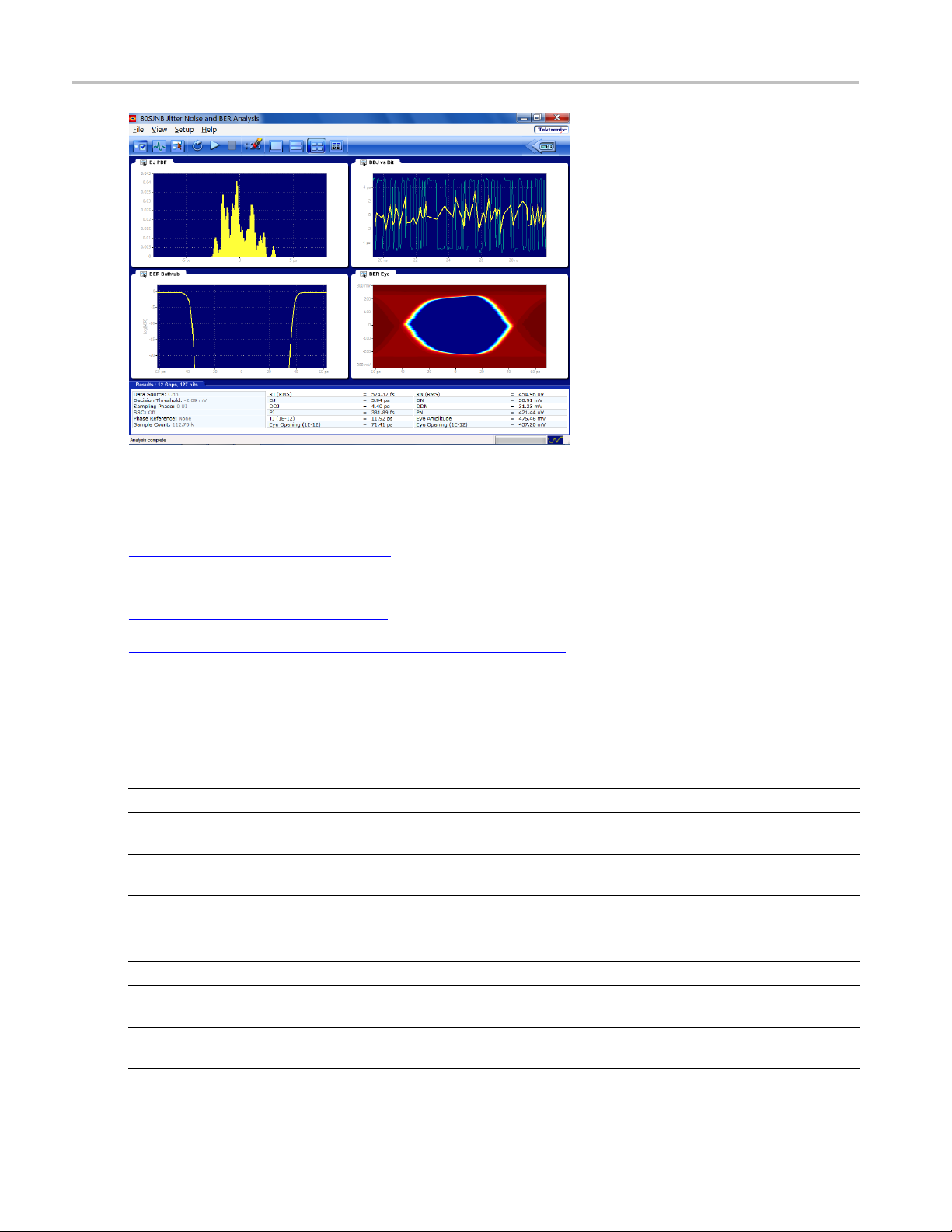
There are two ways to view analysis results: as numeric data and as graphical plots.
You can log the results data to .csv files for viewing in a spreadsheet, database, text editor or data analysis
program.
See Also:
orking with Results
W
Clearing Results (see page 19)
Exporting Plot Files (see page 52)
(see page 13)
(see page 61)
18 80SJNB Printable Online Help

Operating Basics Clearing Results
Clearing Results
Click the Clear Data button to remove the existing plot displays and results. You may want to clear
the data before acquiring new data or between cycles when the sequence mode is set to Free run.
NOTE. The numeric results and plot files are erased each time a new acquisition cycle is started.
About Plotting
The application displays the results as plots for more comprehensive analysis. Before or after you take
measurements, you can select to display a single plot, two plots or four plots. You can select the type
of data you want to view in each plot window.
See Also
Working with Plots (see page 50)
Plot Type Definitions (see page 50)
About Working with Results (see page 61)
:
About the User Interface
The application uses a Microsoft Windows-based user interface.
NOTE. The TekScope application is hidden when the 80SJNB application is running and not minimized.
80SJNB Printable Online Help 19
Operating Basics User Interface Items Definitions
See Also:
Starting the Application (see page 11)
Minimizing and Maximizing the Application (see page 13)
Exiting the Application (see page 14)
Definitions of the application user interface items (see page 20)
User Interface Items Definitions
Item Description
Area
Box
Browse
Check box
Command button Initiates an immediate action, such as the Start command
Keypad
Menu
Menu bar
Visual frame that encloses a set of related options
Usetodefine an option; enter a value with the Keypad or
a Multipurpose knob
Displays a window where you can look through a list of
directories and files
Use to select or clear an option
button in the Control panel
On-screen keypad that you can use to enter numeric values
All options in the application window (except the Control
panel) that display when you select a menu bar item
Located along the top of the application display and contains
application menus
20 80SJNB Printable Online Help

Operating Basics About Navigation
Item Description
Status bar Line located at the bottom of the application display that
shows the acqu
message
Virtual keybo
Scroll bar Vertical or horizontal bar at the side or bottom of a display
Tool bar
xxx
ard
On-screen keyboard that you can use to enter alphanumeric
strings, such as for file names
area that yo
Located alo
application quick launch buttons
isition status and the latest Warning or Error
u use to move around in that area
ng the top of the application display and contains
About Navigation
The application provides you with several ways to display the results:
The drop-
down menus available in the menu bar allows for screen configuration (one, two, or four
plots, summary or full numeric results table)
The butt
ons in the tool bar allow for screen configuration
The drop-down menus available in the plot display windows allow you to choose from the available
and Copy, Examine, and Export plots
plots,
The status bar at the bottom of the screen contains progress information and displays error conditions
ted
detec
Double clicking on a displayed graph opens the plot in a MATLAB window. MATLAB provides
tional display capabilities such as panning, zooming, data cursors, and 3D rotation. The Examine
addi
button from the drop-down menu of the plot also opens the MATLAB window.
80SJNB Printable Online Help 21

Operating Basics About the 80SJNB Tool Bar
See Also:
Windows User Interface (see page 19)
About the 80SJNB Toolbar (see page 22)
About Configuring the Application for Analysis (see page 24)
About the 80SJNB Tool Bar
The toolbar provides quick access to the most common functions you need to configure the settings, start
the acquisition, and control the numerical and plot displays. Most tasks are also available using the
drop-down lists from the File menu bar.
Acquisition button . Use the Acquisition button to select and configure the source for
measurements and control key oscilloscope setups. Any change in the Acquisition settings clears all
the data. The Acquisition button is disabled during the acquisition and processing cycle.
Signal Path button . Use the Signal Path button t o d efine the signal path characteristics to
simulate the actual conditions your signal may encounter. Changes made in the signal path settings
does not clear the data, only the results. The Signal Path button is disabled during the acquisition
and processing cycle.
Analysis Setup button . Use the Analysis Setup button to change settings that affect how
measurements are made and displayed. Changes made in the analysis settings does not clear the data,
only the results. The Analysis Setup button is disabled during the acquisition and processing cycle.
Free Run On/Off button . Use the Free Run button to select the sequence mode (free run on
or off).
When OFF, the button remains blue and the acquisition and processing cycle completes one pass
over the entire pattern. Off is the default mode.
When Free Run is ON, the button turns green
cycle repeats until stopped. The correlated components are averaged with previous data while the
uncorrelated components are accumulated for increased statistical content. At the completion of each
acquisition cycle, the plots and measurements are updated.
indicating that the acquisition and processing
Free Run mode is recommended when:
There is a doubt that one acquisition cycle is enough. A change in the results indicate that additional
acquisition cycles was needed.
22 80SJNB Printable Online Help

Operating Basics About the 80SJNB Tool Bar
The correlated waveform shows irregular disturbances. It is possible that uncorrelated information
can leak into the single-pass c orrelated filtering. Acquiring a larger statistical sample improves
analysis in th
e presence of crosstalk.
To h a lt a F r e e
Sequence mode, so that the acquisition stops when the cycle is complete.
Run button . Use the Run button to start the acquisition and processing cycle. Once the run
button is pressed, do not change any instrument settings. When the Run button is pressed, all current
measurement data and plot displays are cleared. During the acquisition and processing cycle, the
Signal Path, Analysis, Acquisition, and Run buttons are disabled.
During the acquisition and processing cycle, the Run button is replaced with the Pause button
Click Pause to interrupt the current acquisition and processing cycle. Click the button again to resume
the cycl
and processing cycle so you can view and save the measurement data between cycles.
Stop button . Use the Stop button to end the acquisition and processing cycle. While in Single
Sequence mode, stopping the cycle produces no results and you must click the Start button to start a
new cycle.
Clear Data button . Use the Clear Data button to clear all results and plot displays. If Free Run
is set to ON (cumulating previous data with new), you can clear the existing results and plots during
the processing cycle, thus starting a new acquisition and processing cycle.
Plot Display . Use the window pane buttons to display between 1, 2, or 4 plots. You
can
Run cleanly, deselect the
e. This is useful when the acquisition is set to Free Run, allowing you to halt the acquisition
change the number of plot displays at any time.
button. This converts the Free Run mode back to Single
.
meric Results Display
Nu
If the application is displayed on a larger screen, the numeric results display shows all the results at
once.
Back to Scope . Use this button to bring the TekScope display to the front of the screen.
ee Also:
S
About Configuring the Application for Analysis (see page 24)
About Analysis Settings (see page 43)
. The results button changes the display to a complete list of statistics.
80SJNB Printable Online Help 23

Operating Basics MATLAB User Interface
MATLAB User Interface
The 80SJNB application includes MATLAB®plots to provide further data analysis and visualization of
the plot displays.
MATLAB provides multiple capabilities to display and annotate the plot diagrams, including:
Pan and Zoom
2D and 3D visualization
Rotation
Data Curso
Color enhancements
MATLAB is a product distributed by MathWorks. You can view the MATLAB documentation and
tutorials on their Web site: http://www.mathworks.com
rs
About Configuring the Application for Analysis
The tool bar provides an Acquisition (see page 25) button to configure the application to acquire data,
a Signal Path
to change settings that affect how measurements are made and displayed.
NOTE. The Acquisition settings must be set before starting an acquisition cycle. You can modify the Signal
Path and Analysis settings without the need to reacquire data.
24 80SJNB Printable Online Help
(see page 33) button to set signal path conditions, and an Analysis (see page 43) button

Operating Basics About Acquiring Data
Use the Sequenc
run) or stop after one cycle is complete.
After setting up the application, you can select the Run button
cycle.
After the acquisition and processing cycle has completed, you can view the results as numerical
page 61) statistics or graphically (see page 19).
e button
About Acquiring Data
Before making jitter and noise measurements, you need to select and configure the signal source.
Use the Acquisition button
In the Acquisition dialog box, select the signal source and define the acquisition parameters. Some
parameters (such as the Clock Recovery, Phase Reference Sources, and the optical signal conditioning)
are copied from the oscilloscope state.
Click the AutoSync to Selected Source button to have the 80SJNB application automatically obtain and
enter the following information from the signal applied to the channel defined as the Signal Source:
Data Pattern Rate
to have the acquisition and processing of data run continuously (free
to start the acquisition and processing
(see
to display the Acquisition dialog box.
Data Pattern Length
mmended Data:Clock Ratio (when Spread Spectrum Clocking (SSC) signaling is used)
Reco
NOTE. Acquisition in the presence of SSC requires certain cabling propagation delays to be preserved.
Please contact Tektronix for an up-to-date diagram of cabling lengths.
NOTE. Tektronix recommends running this functionality in the oscilloscope (the equivalent menu exists in
Setup > Mode/Trigger > Pattern Sync/FrameScan Setup). The important difference is that the oscilloscope
UI/PI allows manual entry of some of the parameters of the AutoSync, which dramatically improves the
success rate of AutoSync. For example, manually entering the Data Pattern Length, and then unchecking
the pattern length item from the AutoSync search, makes the data pattern length much more likely to
ucceed. Refer to the DSA8300 TekScope application online help for details about the Pattern Sync settings.
s
80SJNB Printable Online Help 25

Operating Basics Selecting Clock Recovery
See Also:
Selecting the Source (see page 30)
Selecting the Data Pattern (see page 29)
Selecting the Pattern Sync (see page 30)
Selecting the Signal Conditioning (see page 29)
ting Clock Recovery
Selec
Selecting Phase Reference (see page 28)
Analysis Settings (see page 43)
(see page 26)
Selecting Clock Recovery
The Advanced Trigger option (ADVTRIG) that generates the pattern synchronous triggers requires a clock
source synchronous with the signal. When using a clock derived from a clock-recovery module installed
in the oscilloscope (such as optical modules and the 80A05), use the Pattern Clock fields to select the
urce module, the configuration and its frequency.
so
26 80SJNB Printable Online Help
Operating Basics Selecting Clock Recovery
All native clock recovery modules support two different configurations: one that connects the recovered
clock from the back of the module to the internal pattern synchronous trigger generator; and, for optimal
jitter performance, t he module full rate clock output can be connected to the front panel Clock/Prescale
Input.
These settings are grayed out if no modules with clock recovery are detected at application startup.
The Rate setting is limited to the capabilities of the selected module. The numeric keypad is unavailable
for use unless the module can accept USER defined rates.
80SJNB Printable Online Help 27
Operating Basics Selecting Phase Reference
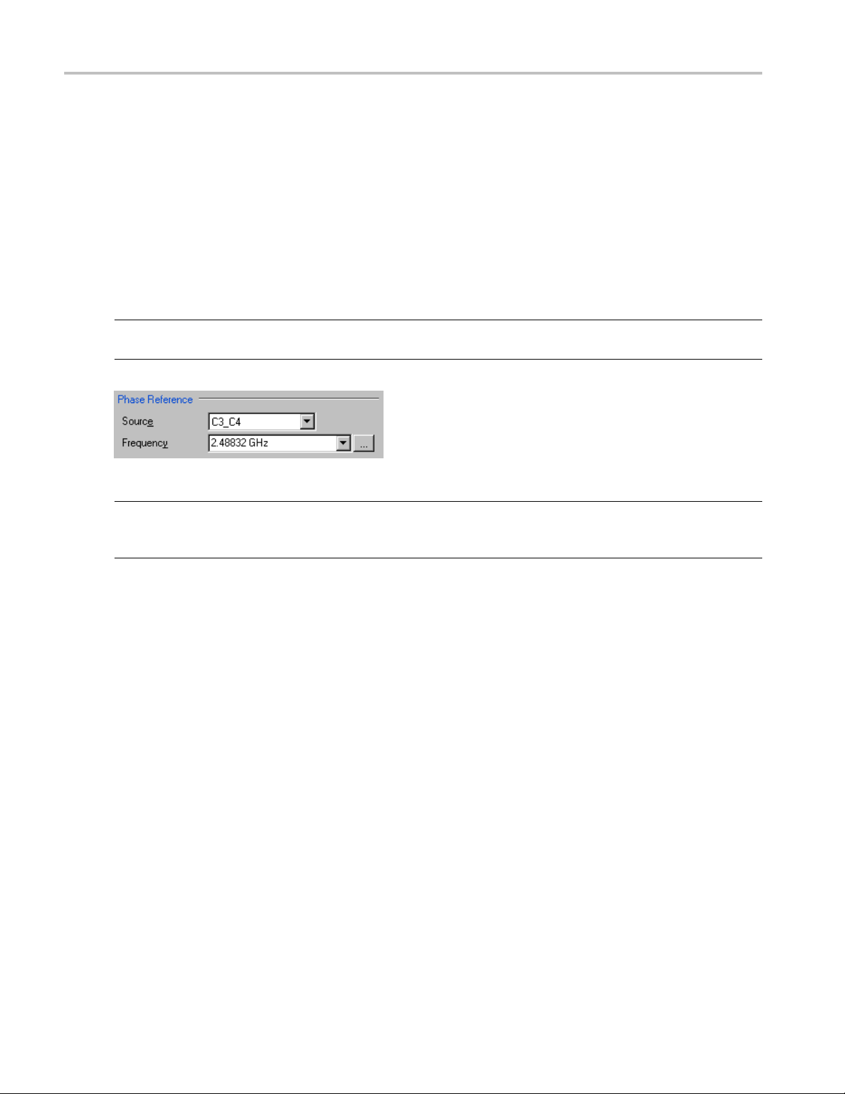
Selecting Phase Reference
You can use a Phase Reference module (such as the 82A04) to reduce the trigger jitter of the signal source,
thus increasing the jitter measurement accuracy. If analyzing a signal using Spread Spectrum Clocking
(SSC), a Phas
If using a Phase Reference module, set the channel source and the frequency of the applied clock.
These settings are grayed out if a Phase Reference module is not detected at application startup. If a Phase
Reference module is detected, you have the option to not use the module by selecting None as the Source.
e Reference module is required.
TIP. Selec
Jitter) and the correlated waveforms. However, the throughput is lowered in this mode.
NOTE. W
frequency when the data was acquired. The Source field remains unchanged regardless if phase reference
was used when the recalled data file was created.
ting a Phase Reference module dramatically improves the accuracy of DDJ (Data Dependent
henusingarecalleddatafile, the Phase Reference Frequency field is updated to indicate the
28 80SJNB Printable Online Help
Operating Basics Selecting the Data Pattern
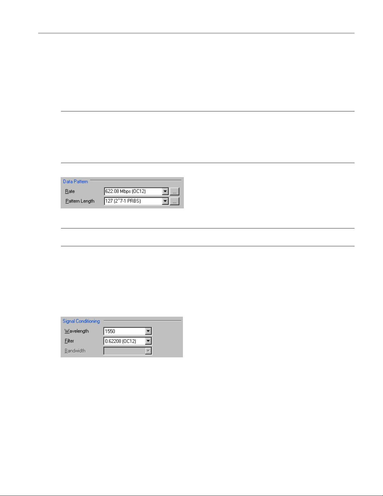
Selecting the Data Pattern
Defining the Data Pattern requires that you define both the data rate of the signal source and the pattern
length in bits. You can choose the data rate from a predefined set of lengths or enter a value with the
numeric keyp
NOTE. Selecting a data rate that does not match the communication standard that is set in the instrument’s
Horizontal Communication Standard setting dialog box causes the oscilloscope setting to change to User.
When selecting the pattern length, only the length is important. The precise bit sequence is unimportant
if it is repetitive.
To analyze a clock pattern, select a 2 bits pattern (or a multiple). The analysis is performed on both edges.
ad.
Sele
NOTE. W
settings when the data was acquired.
henusingarecalleddatafile, the Data Pattern fields are updated to indicate the state of the
cting the Signal Conditioning
his control to select what type of filtering, if any, you want performed on the selected channel. The
Use t
available filters depend on the capabilities of the module.
If the Filter is set to None, you can use the Bandwidth box to select the bandwidth of the channel. The
available bandwidth selections depend on the capabilities of the module. Refer to the documentation for
he module about its filter or bandwidth settings.
t
80SJNB Printable Online Help 29
Operating Basics Selecting the Pattern Clock
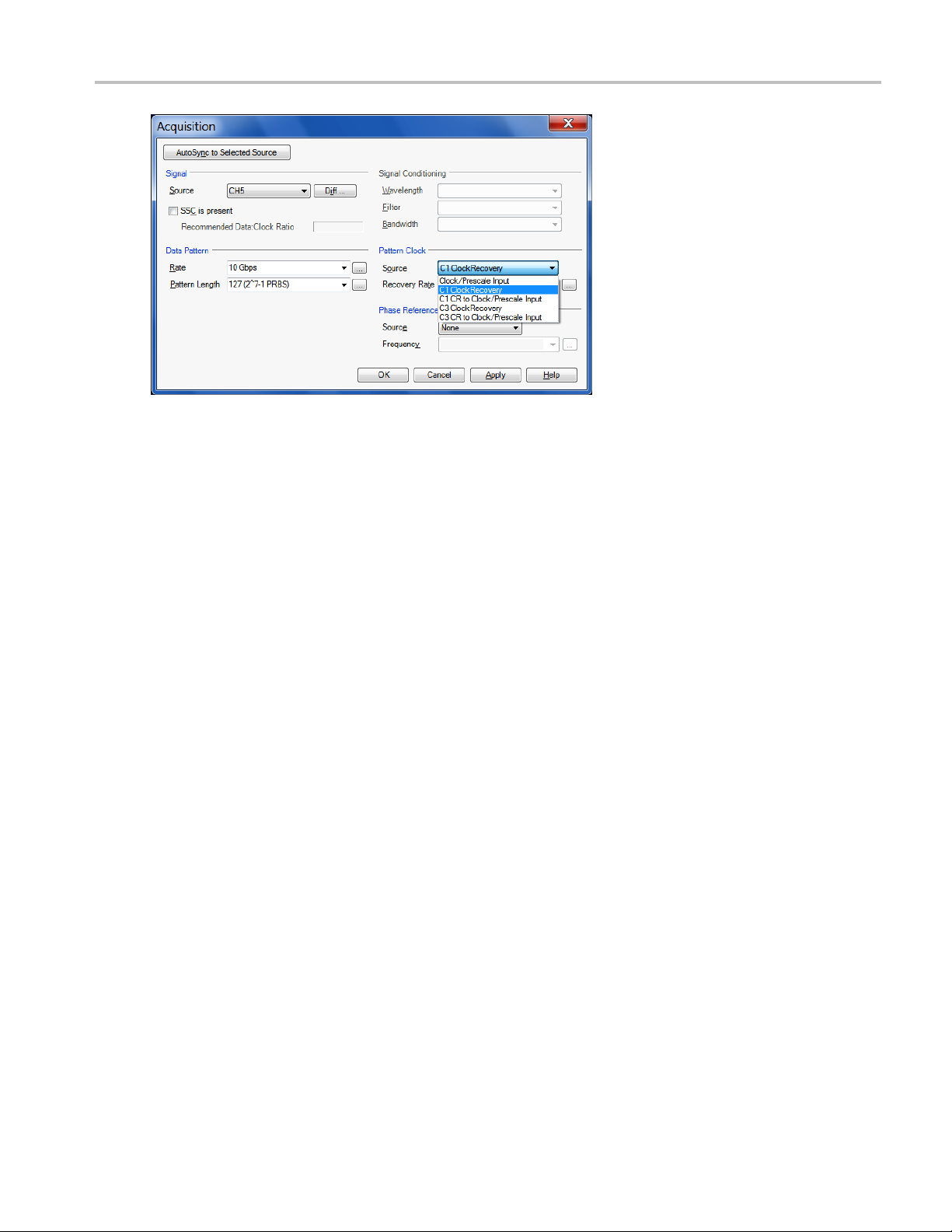
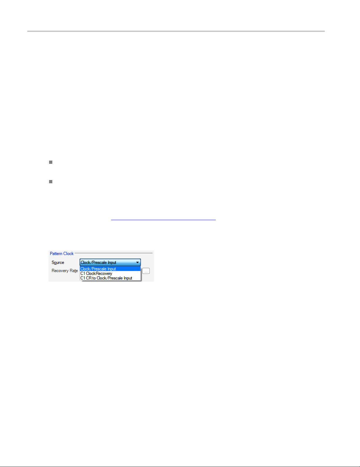
Selecting the Pattern Clock
The Pattern Sync built-in capability provides user pattern synchronous triggers. The feature, enabled by
the Advanced Trigger Option (ADVTRIG), is driven by the Pattern Clock.
The available Pattern Clock sources depend on the instrument configuration. The default selection is
Clock/Prescale Input, and this selection is available for all configurations. Connect the clock source to
the CLOCK IN
When the oscilloscope is equipped with one or more clock recovery capable modules, the CR units are
also avail
Each native clock recovery source appears on the Pattern Clock source list twice to allow for two different
configura
Selecting Cx Clock Recovery sets the instrument to pick up the recovered clock from the back
of the mo
Selecting Cx CR to Clock/Prescale Input sets the instrument clock recovery signal source to the
CLOCK I
recovery module to the front panel CLOCK INPUT/PRESCALE TRIGGER input.
PUT/PRESCALE TRIGGER front-panel connector.
able as sources for the Pattern Clock.
tions:
dule using and internal signal path.
NPUT/PRESCALE TRIGGER connector on the front panel. Connect the output of the clock
Depend
jitter performance. See Selecting Clock Recovery
particular cabling setup is necessary; only external Clock Recovery (such as with a CR125A) can be used.
If the PhaseRef 82A04 module is used in the absence of SSC, the 82A04 setup determines the jitter
performance. The intrinsic jitter of the pattern trigger circuit becomes invisible.
ing on the data rate, choosing one configuration over the other could result in different intrinsic
Selecting the Source
The application takes measurements on waveforms specified as sources (also called signal sources). The
source can be a channel (CH1 through CH8) or a math waveform (if one is defined). You can use any
defined math waveform, whether it is definedinthe80SJNBconfiguration as a differential setup or in
the TekScope application. (Defining a math waveform in the TekScope application must be done before
launching the 80SJNB application.)
(see page 26). In general, if there is SSC then a
When selecting a Data Source, all other channels and Math waveforms should be turned off. If any
channels or Math, other than the Data Source are activated after launching the 80SJNB application, an
error message will prompt you to deactivate all additional waveforms before starting the acquisition and
processing cycle. All other waveform databases, measurements, histograms and masks on the oscilloscope
30 80SJNB Printable Online Help

Operating B asics Selecting the Source
need to be turned off, as well. If any of these conditions exist when starting the acquisition and processing
cycle, you are prompted to turn these off before you can continue.
If your signal source uses Spread Spectrum Clocking (SSC), select the check box so that the application
can make accurate measurements accounting for clock rate modulation.
NOTE. If a sav
panels will indicate the recalled data file as the source. The “SSC is present” field is updated to match
the setting from the recalled data file.
ed data file is recalled, the signal source selection remains unchanged but all result
See Also:
About Spread Spectrum Clocking (SSC) (see page 32)
Clicking the Diff button displays the dialog box to create a differential Math waveform by defining a
positive and negative waveform source (the negative waveform source is subtracted from the positive
waveform source). This generates a single mathematical waveform that the 80SJNB application can use
as the waveform measurement source.
TIP. You can use the DSA8300 TekScope Define Math dialog box (Edit > Define Math) to define more
complex math expressions. You must define the math expression in the DSA8300 before launching the
80SJNB application. Refer to the online help for your oscilloscope.
80SJNB Printable Online Help 31

Operating Basics About S pread Spectrum Clocking (SSC)
About Spread Spectrum Clocking (SSC)
Spread Spectrum Clocking (SSC) is the technique of modulating the clock frequency to minimize EMI
effects. SSC affects the analysis process and the results of jitter, noise and BER measurements. If SSC
is not correc
reflected in the total jitter and noise, and ultimately in the BER estimates.
ted for its effects, the results show as a large amount of periodic jitter components that are
When SSC is p
resent, 80SJNB measures the attributes of SSC and corrects the results.
Configuration Requirements
If using clock recovery, the clock recovery unit must be able to handle SSC. Use one of the Tektronix
BERTScope clock recovery instruments if SSC is present in the signal.
TheTekScopemusthavean82A04PhaseReferenceModule installed. The module minimizes the effect
of the SSC on the data by sampling synchronously the data and clock. Also, by acquiring the clock in the
82A04 module, 80SJNB characterizes the SSC present intheclockandusesthatinformationtocorrectthe
jitter, noise, and BER measurements performed on the data.
TIP. The “SSC is present” check box is disabled if the Phase Reference module is not installed in the
ment.
instru
Use the following settings to optimize the SSC phase correction for the signal you are measuring:
Clock recovery
Data rate ran ge
500 Mbps – 1 Gbps Data Rate * 4 Standard
1 Gbps – 2 Gbps Data Rate * 2 Standard
2 Gbps – 4 Gbps
4 Gbps – 8 Gbps
8 Gbps – 12.5 Gbps
xxx
1
The Clock Recovery unit clock output is either Standard or Subrate Clock.
2
Clock recovery is typically provided from a CR125A, CR175A, or CR286A BERTScope Clock Recovery Instrument.
frequency
Data Rate
Data Rate
Data Rate
2
Clock recovery
output rate
Standard
Subrate (1/2)
Subrate (1/4)
1,2
When you instruct 80SJNB that the data has SSC (by checking the “SSC is present” check box), the
following constraints are enforced based on the current Data Rate:
Data:Clock ratio
(JNB)
1:4
1:2
1:1 Data Rate
2:1
4:1
Phase reference
frequency (JNB)
Data Rate * 4
Data Rate * 2
Data Rate/2
Data Rate/4
Phase Reference source is selected.
Phase Reference frequency is set to the recommended value in the table Configuration Settings for SSC.
A recommended Data:Clock Ratio is displayed to suggest the recommended subrate clock.
NOTE. Changes to the Data Rate are reflected in the Phase Reference Frequency and Data:Clock Ratio.
You must make the appropriate changes to the Clock Recovery unit parameters.
32 80SJNB Printable Online Help

Operating Basics About Serial Data Link Analysis (SDLA) Signal Path Settings
The status (on or off) of the SSC setting is displayed in both the Summary – SSC view and the Full
Numeric Results page. The results of the SSC analysis are p resented in two forms, numeric results and a
plot. When vie
and Frequency. Magnitude represents the depth of the SSC clock modulation in parts-per-million (ppm)
and Frequency reflects the SSC modulation frequency.
To view the plot of the SSC modulation profile, select the Plot>SSC>SSC Profile.
wing the full numeric results table, the SSC Modulation section has two fields: Magnitude
TIP. The
oscilloscope. Refer to the information provided with the oscilloscope.
configuration settings are also available through the GPIB programming interface of the
About Serial Data Link Analysis (SDLA) Signal Path Settings
The Signal Path Settings are available for use with the 80SJNB Advanced version. If you are using the
80SJNB Essentials version, you're allowed to use the dialog boxes but are not allowed to place any
of the functions into the signal path.
The Signal Path settings allow you to emulate the environment your signal encounters, all the way from
the transmitter to the receiver. With the Signal Path dialog box, your signal path is represented by a line
the transmitter (Tx) to the Receiver (Rx). Along this line, you have the ability to emulate an arbitrary
from
filter and/or a channel. You can then define an equalizer to compensate for the effects the filter and channel
introduce. Also, fixture de-embed is supported.
Selecting a signal path arrow (Filter, Channel, or Equalizer) inserts or removes the function from the signal
path. When inserting a function into the signal path, its dialog box automatically displays.
Selecting a signal path button (Filter, Channel, or Equalizer) displays the dialog box for that function
without inserting or removing the function from the signal path.
80SJNB Printable Online Help 33

Operating Basics Setting Filter Conditions
By simulating the signal environment, you can effectively emulate probing the signal at the receiver rather
than the output of the transmitter. With the use of the Equalizer, you can then design compensations to
improve the signal quality at the receiver.
TIP. You can move a function in and out of the signal path without affecting any settings.
To learn more about each of the signal path settings, select the following:
(see page 34)
Filter
Channel (see page 35)
Equalizer (see page 37)
Setting Filter Conditions
The Signal Path Filter allows you to specify an arbitrary linear FIR filter to be applied to the acquired
data pattern. For instance, the transmitter may artificially enhance the signal at certain frequencies to
overcome known problems in the channel. You can use a filter to emulate this action or compensate for
transmitter signal pre-emphasis.
To use the filter, move the Filter function into the signal path and use the Filter file box or browse button to
specify the filter file. The default location for the filter files is in the Windows/Documents folder. A few
filter files are provided as examples, but you are responsible for providing the filter files.
To use the Filter block for de-embedding, you will need an additional software tool to create a
de-embedding filter from the S-parameters of the fixture. Please visit the www.tektronix.com/sdla
site, or contact Tektronix Support for details.
Web
See Uncorrelated Scaling (see page 42) for information about this setting.
The following is an example of the filter file format:
34 80SJNB Printable Online Help

Operating Basics Setting Channel Conditions
#Thisisasamplefilter file. The '@' means that it is valid for all frequencies.
#Upto20,000coefficients may be specified.
@ 5.7e-005, 2.
4e-005, 5.4e-005, 2.1e-005, 5.1e-005
Setting Channel Conditions
The Signal Path Channel allows you to emulate the channel (interconnect or lane) carrying the signal.
There are two ways to define the channel, with Time Domain
Domain (see page 35) S-parameters.
(see page 37) waveforms and Frequency
See Uncorrelated Scaling
Frequency Domain
With Frequency Domain selected, the channel is defined with an S-parameters file. Use the file selection
box or Browse button to select the file. The default location for the files are in the Windows/Documents
folder. You are responsible for providing the S-parameters file.
The S-parameters file can contain data for 1-port, 2-port, or 4-port devices. Once a file is selected,
the application reads its contents and generates the appropriate dialog for you to select the particular
S-parameter in the file to use.
(see page 42) for information about this setting.
1-Port. Files with 1 port of data contain only 1 S-parameter so they do not require any further input. These
es may be IConnect 1-port files or Touchstone 1-port files.
fil
2-Port. Files with data for 2 ports contain 4 S-parameters as a 2x2 matrix. These are Touchstone 2-port
files. When the application recognizes such an S-parameter file, a dialog is created for you to select the
S-parameter representing channel transmission. The typical selection is S
but this may need to be changed if the file contains a 2x2 subset of the 4x4 matrix of S parameters defining
a4-portsystem.
80SJNB Printable Online Help 35
, and is the default selection,
21

Operating Basics Frequency Domain
4-Port. Fi
les with data for 4 ports may contain single-ended or mixed-mode data. These are Touchstone
4-port files.
If the data
link. A default mapping is assumed. The application will use this mapping to compute the S
is single ended, you must map the port numbers as used in the file to physical locations in your
parameter
dd21
(for transmission of a differential signal) from the appropriate four S-parameters measured using single
ended data.
If the data is mixed mode, you must select the data layout in the file. The most common layout is DC12
and is the default selection. The application always uses the S
parameter for computing the transmitted
dd21
waveform no matter which mapping is selected.
NOTE. 80SJNB Advanced uses the 'insertion loss' information only.
36 80SJNB Printable Online Help

Operating Basics Time Domain
Time Domain
With Time Domain selected, the Reference waveform and Transmitted waveform generate the channel
behavior. Use the file boxes or browse buttons to select the files you want to use. The default location
for the files i
waveform files.
NOTE. We recommend that the waveform file be a measurement of the channel from a Tektronix TDR/TDT
system. Required raw oscilloscope waveforms are:
a. A reference throughput (no DUT is inserted, just a throughput connection between the TDR step
source and the acquisition channel on the TDT end).
b. A DUT throughput measurement (the TDR step source and the TDT acquisition channel are connected
through the DUT).
s in the Windows/Documents folder. You are responsible for providing the time domain
About the Equalizer
The equalizer compensates for transmission channel impairments in the form of frequency-dependent
amplitude and phase distortions resulting in intersymbol interference (ISI) in the communication data
stream.
80SJNB provides tools to define an equalizer by a set of Taps or weights. The linear feed-forward
equalizer (FFE) is defined by a user specified number of taps, taps per symbol (or unit interval), and the
weight of each tap. The equalizer becomes a decision-fe edback e qualizer (DFE) when the number of DFE
taps is set to a number larger than 0.
OTE. Tap values and weights are used interchangeably.
N
80SJNB Printable Online Help 37

Operating Basics Equalizer Taps
To learn about setting up the Equalizer, see:
Equalizer Taps
Uncorrelated Scaling (see page 42)
Equalizer Taps
The behavior of the equalizer is controlled by the number of taps and the tap values. Using the equalizer
requires that you specify the number of FFE and DFE taps, and the FFE spacing of the taps. You can also
incorporate an equalizer fi lter delay by specifying a reference tap to compensate for precursor channel
effects.
You can manually set the FFE and DFE tap values, or you can use the Autoset Taps button to let the
application calculate the tap values.
(see page 38)
38 80SJNB Printable Online Help

Operating Basics Equalizer Taps
Go to FFE Taps description (see page 39)
Go to DFE Taps description (see page 40)
FFE Taps
The FFE Taps are weights applied to a set of samples taken from the data stream to compensate for
channel impairments manifested in the form of ISI. The number of FFE Taps represent the length of
history
be distanced at unit intervals, in which case the number of FFE taps represents the number of preceding
bits that contribute to the correction of the current bit. Alternatively, the data stream could be sampled
at a higher rate per bit, yielding a fractionally-spaced FFE tap set.
in data samples that contribute to the computation of a current bit. Data stream samples could
The number of FFE taps defaults to 1, with the capability to specify up to 100 taps. The default FFE tap
spacing is at unit intervals. You can configure up to 10 taps per symbol.
The FFE Tap values could be specified by you using the FFE Taps dialog, or computed by the application
with the Autoset Taps button.
Go to Autoset Taps description
Go to Saving and Loading Taps (see page 42)
Pressing the FFE Taps button displays a dialog showing the current FFE tap values. You can specify each
FFE tap coefficient individually. Pressing the Defaults button sets the first FFE tap to 1 and the rest to 0.
(see page 41)
80SJNB Printable Online Help 39

Operating Basics Equalizer Taps
You can use the Save Taps button to save a set of coefficients to a file. Use the Load Taps button to load
saved Tap files.
DFE Taps
DFE taps are weights applied to the previous digital decisions made by the slicer (comparator + latch). The
number of
number of DFE Taps is 0, in which case the equalizer is a linear FFE one. The maximum number of DFE
Taps is 40. Weights are scalars specified by you or computed by the Autoset Taps function.
DFE Taps specifies the number of bits contributing to the current input to the slicer. The default
See Autoset Taps
ng the DFE Taps button displays a dialog showing the current DFE tap values. You can specify each
Pressi
DFE tap coefficient individually. Pressing the Defaults button sets all DFE tap values to 0.
You can use the Save Taps button to save a set of coefficients to a file. Use the Load Taps button to
recall saved Tap files.
TIP. When using the Equalizer, you are required to always have at least 1 FFE tap. DFE taps are optional.
(see page 41) for a description about using the autoset taps function.
Filter
40 80SJNB Printable Online Help

Operating Basics Autoset Taps
FFE Reference Tap. The FFE Reference Tap is a filter delay in unit intervals that should be set to
compensate for the delay between the transmitter output and the equalizer input. The value of the
Reference Tap
is constrained by the number of FFE Taps and the number of taps per symbol.
Rise Time Selector. TheRiseTimeSelectorspecifies the Gaussian filter used to emulate the DFE feedback
path band-limited behavior. The rise time defaults to Track Data Rate, in which the configuration is
set to 1/5 of the unit interval equivalent with the data rate. Track tap interval designs a Gaussian filter
with a rise equal to 1/5 of the spacing between taps. Selecting User allows you to specify the rise time
from1psto4
ns.
Uncorrelated Scaling. See Uncorrelated Scaling
Autoset Taps
The tap autoset function computes a set of tap values that optimize the eye opening for the data pattern
applied to the input of the equalizer. If the DFE tap number is 0, the algorithm yields an optimal set of FFE
taps, while if the equalizer is specified as a DFE by a positive DFE tap number, the Autoset Taps algorithm
jointly optimizes the forward and feedback loop tap coefficients. The optimization algorithm is the
least-mean-square e rror (LMS) and the optimization targets the signal to noise ratio at the sampling phase.
The Autoset Taps will account for the FFE Taps/Symbol and Reference Tap specifications.
The autoset algorithm assumes the availability of a training sequence, thus it supports only a known set of
patterns:PRBS3toPRBS15withthefollowing generator polynomial equations:
PRBS3: x
S4: x
PRB
PRBS5: x
PRBS6: x
PRBS7: x
PRBS8: x
PRBS9: x
RBS10: x
P
PRBS11: x
PRBS12: x
PRBS13: x
PRBS14: x
PRBS15: x
3+x2
+1
4+x3
+1
5+x4+x2+x1
6+x5+x3+x2
7+x6
+1
8+x7+x3+x2
9+x5
+1
10+x7
+1
11+x9
+1
12+x9+x8+x5
13+x12+x10+x9
14+x13+x10+x9
15+x14
+1
(see page 42) for a description o f this control.
+1
+1
+1
+1
+1
+1
The tap autoset algorithms computes a set of FFE and DFE taps using a least-mean-square optimization
algorithm. The optimization algorithm is the least-mean-square error (LMS) and the optimization targets
the signal to noise ratio at the sampling phase.
NOTE. You can autose t tap values even if the Equalizer is not inserted in the signal path.
80SJNB Printable Online Help 41

Operating Basics Saving and Loading Taps
Saving and Loading Taps
Use these controls to save or load a set of taps from a file. The browse directory defaults to Windows/My
Documents and the file extension is .tap.
The file format is the following:
<Tektronix>
<TapFile>
<FFE>
<TapsPerS
<ReferenceTap>value<\ReferenceTap>
<Tap1>value<\Tap1>
<Tap2>value<\Tap2>
...
<Tapn>value<\Tapn>
</FFE>
<DFE>
<Tap1>value<\Tap1>
<Tap2>value<\Tap2>
...
<Tapn>value<\Tapn>
</DFE
</TapFile>
</Tektronix>
>
ymbol>value<\TapsPerSymbol>
Uncorrelated Scaling
The signal path settings (Filter, Channel, Equalizer) each have an uncorrelated scaling setting. The
Uncorrelated Scaling value multiplies the uncorrelated random noise RMS and uncorrelated periodic noise
values. Uncorrelated noise scaling affects the uncorrelated jitter as projected through the average slew rate.
The 80SJNB Signal Path does not process uncorrelated noise in any other way.
If you insert a default equalizer (an FFE Tap 1 value equal to 1, and zero DFE taps) in the Signal Path
and set the Uncorrelated Scaling factor to its minimal value (0.01), the configuration will isolate the
effects of noise on jitter measurements. This configuration produces results that correlate with “jitter
only”typeanalysistools.
NOTE. The overall Signal Path uncorrelated scaling factor is the product of all signal path uncorrelated
scalar values of the active functions.
42 80SJNB Printable Online Help
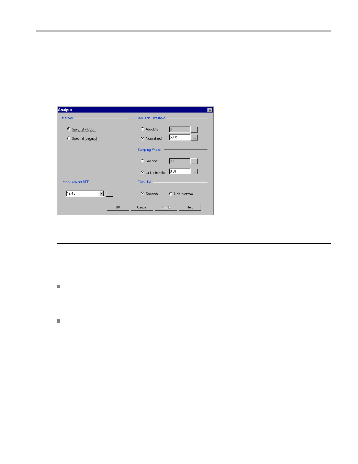
Operating Basics About Analysis Settings
About Analysis Settings
The Analysis settings affect how measurements are made and displayed. The settings are saved with the
80SJNB application whenever it is closed so that restarting the application results in using the same
settings.
TIP. Changes to Analysis settings are reflected in the current plots and results.
Setting the Analysis Method
The Method selection sets which analysis methodology to use for the Jitter and Noise breakdown:
The Spectral + BUJ (Bounded Uncorrelated Jitter) is using a combination of spectral isolation of
the periodic components and the analysis of the cumulative distribution function (CDF) of the
uncorrelated jitter and noise data, before and after spectral separation. The presence of crosstalk
dictates the selection of this method.
The Spectral (Legacy) mode relies on spectral separation of the periodic and random components.
The default setting is Spectral + BUJ. When switching the analysis method between the two options, the
acquisition data is preserved, and new results are recomputed, displayed, and plots made available.
Setting the Decision Threshold
The Decision Threshold specifies the level at which to determine the crossing points on the edges of the
measured waveform.
When set to Absolute, the decision threshold uses the absolute value provided in volts (electrical) or
watts (optical).
80SJNB Printable Online Help 43

Operating Basics Taking Measurements
When set to Normalized, the decision threshold is calculated based on waveform data according to the
percent value of the signal amplitude.
Setting the Time Unit
The Time Unit sets the units (Seconds or Unit Intervals) used when displaying the measurement results.
Setting the Sampling Phase
The Sampling Phase determines the location of the sampling point for the Vertical Eye Opening and all
correlated noise measurements within the bit interval.
When set to Seconds, the sampling point uses the absolute value entered. Zero seconds is at the center of
the bit interval.
When set to Unit Intervals, the sampling point is calculated based on the bit interval. Zero UI is the
center of the unit interval.
Setting the Measurement Bit Error Rate
The Measurement BER determines the rate for which the measurements (such as TJ@BER) are predicted.
Taking Measurements
You should return the oscilloscope to its default state before launching the 80SJNB (acquisitions and math
waveforms should be off, and all
should not have to make changes to the oscilloscope settings from the oscilloscope UI to successfully
acquire data with the 80SJNB application. The most relevant oscilloscope settings are accessible using the
Configuration dialog box of the 80SJNB application.
Displaying Measurements
You can use the tool bar to select how the results are displayed: numeric results, plots (up to four), or a
combination.
What do you want to do?
Display the definitions of Jitter measurements
Display the definitions of Noise measurements (see page 46)
measurements, waveform databases, masks, and histograms). You
(see page 45)
Measurement Algorithms (see page 93)
Go to Working with Numeric Results (see page 61)
Go to Working with Plots (see page 50)
44 80SJNB Printable Online Help

Operating Basics Jitter Measurement Definitions
Jitter Measurement Definitions
Jitter measurements Description
Random Jitter
RJ (RMS)
RJ(h) (RMS) Horizontal c
RJ(v) (RMS) Vertical co
Determini
DJ Measured Deterministic Jitter
DDJ Data Dependent Jitter
DCD Duty Cycle Distortion
DDPWS Data Dependent Pulse Width Shrinkage
BUJ(d-d)
PJ
PJ(h) Horizontal component of periodic jitter (peak-to-peak)
PJ(v) Vertical component of periodic jitter (peak-to-peak) induced by noise
NPJ(d-d)
Total Jitter @ BER
xxx
stic Jitter
TJ (1E-12) Total Jitter at user-specified BER
Eye Opening (1E-12) Horizontal Eye Opening at user specified BER
Measured Random Jitter
omponent of random jitter
mponent of random jitter induced by noise converted to jitter
through an average slew rate
Measure
Measured Periodic Jitter (peak-to-peak)
converted to jitter through an average slew rate
Measured NonPeriodic Jitter, Dual Dirac model
d Bounded Uncorrelated Jitter, Dual Dirac model
NOTE. J2 Jitter: For a BER specified as 2.5E-3, the Total Jitter becomes J2 Jitter. J2 Jitter measures all
but 1% of the statistical total jitter distribution.
J9 Jitter: For a BER specified as 2.5E-10, the Total Jitter becomes J9 Jitter. J9 Jitter represents an
estimation of all but 10E-9 of the statistical total jitter distribution.
Dual Dirac Measurement Definitions
Dual Dirac D escription
RJ(d-d)
DJ(d-d)
xxx
Random Jitter computed in the Dual Dirac model
Deterministic Jitter computed in the D ual Dirac model
80SJNB Printable Online Help 45

Operating Basics Noise Measurement Definitions
Noise Measurement Definitions
Noise measurements Description
Random Noise
RN (RMS)
1
RN(v) (RMS) Vertical com
RN(h) (RMS) Horizontal
Determini
stic Noise
DN Measured Deterministic Noise
DDN Data Dependent Noise
DDN(level 1)
DDN(level 0)
BUN(d-d)
1
PN
PN(v) Vertic
PN(h) Horiz
NPN(d-d)
Total Noise @ B ER
TN (1E-12) Total Noise at user-specified BER
Eye Opening (1E-12) Eye Opening at user-specified BER
Eye Amplitude
xxx
1
ncorrelated random noise (RN) and periodic noise (PN) measurements are performed on both logical levels 1 and 0 to account for significant
U
differences, which may be the case when the measurements are performed on optical signals.
Measured Random Noise
ponent of random noise
component of random noise induced by jitter
converted to noise through an average slew rate
Data Depe
Data Depe
Measure
Measur
ndent Noise on logical level 1
ndent Noise on logical level 0
d Bounded Uncorrelated Noise, Dual Dirac model
ed Periodic Noise
al component of periodic noise (peak-to-peak)
ontal component of periodic noise (peak-to-peak)
induced by jitter converted to noise through an average slew
rate
Measured NonPeriodic Noise, Dual Dirac model
The amplitude of the eye computed as the mean-to-mean of
gical 1 and logical 0 bit levels sampled at the user defined
lo
Sampling Phase.
SC Modulation Measurement Definitions
S
SSC modulation measurements Description
Magnitude
Spread spectrum clock modulation magnitude of the clock in
parts-per-million (ppm) units.
Frequency
xxx
Spread spectrum clock modulation frequency.
46 80SJNB Printable Online Help

Operating Basics Sample Count
Sample Count
Both results tables, Summary and Full Results are displaying the Sample Count of the data used for the
derivation of the measurements.
The Sample Count field represents the amount of statistical data acquired and analyzed, and contains the
full pattern acquisition, the jitter and noise characterizing data.
When in Free Run, the count is continuously incremented with the newly acquired and processed data.
Steps to Acquire Data
To acquire data from acquisition channels and take measurements, follow these steps:
1. Select
setup an
2. Select
processing cycles. When in Free Run mode, the following acquisition and processing continues
until you stop it:
acquisition and averaging of data-correlated patterns
acqui
3. Sele
To stop the acquisition, do one of the following:
ct
If you wish to stop the acquisition and processing cycle before it completes, select .Thismay
useful if you have started a sequence on a long waveform and then realize you would like to
be
change the configuration.
If you wish to interrupt the acquisition and processing cycle, select . Select a second time to
resume the acquisition.
If you wish to halt a Free Run mode cleanly, toggle the Sequence button. This will convert the
Free Run mode (indicated by the green button) to Single cycle mode (indicated by the blue button) so
that the acquisition stops when the cycle is complete. Single cycle is the default mode.
to display the Acquisition dialog box and configure the application according to your
d signal type.
to toggle the acquisition mode between free run (continuous) and single acquisitions and
sition, accumulation and statistical analysis of uncorrelated data
to start the acquisition and processing cycle.
TIP. Use the Clear Data
80SJNB Printable Online Help 47
button to delete all measurement results and plots.

Operating Basics Saving and Recalling Setup Files
Saving and Recalling Setup Files
You can use the File menus to save and recall different oscilloscope and application setups. Setup files
store the oscilloscope and application settings.
CAUTION. Do n
ot edit a setup file or recall a file that was not generated by the application.
See Also:
Saving a Setup File
Recalling a Saved Setup File (see page 48)
(see page 48)
Saving a Setup File
To save the 80SJNB application and oscilloscope settings to a setup file, follow these steps:
1. Select File > Save Settings to open the Save dialog box.
2. In the file browser, select the directory in which to save the setup file.
3. Use the keyboard to enter a new fi le name. The application appends a .stp extension to the file name.
4. Save the setup file. If the selected file name already exists, a confirmation dialog appears that allows
you to cancel the operation.
NOTE. The application saves the oscilloscope setup.
Recalling a Saved Setup File
To recall the application and oscilloscope settings from saved setup files, follow these steps:
1. Select File > Recall Settings to open the Recall dialog box.
2. In the Recall dialog box, select the directory from which to recall the setup file.
3. Select a setup file name, and then select Open.
CAUTION. Do not manually edit setup files. If you try to recall a setup file that was manually edited, the
recall operation fails.
48 80SJNB Printable Online Help

Operating Basics Saving and Recalling Data Files
Saving and Recalling Data Files
You can use the File menus to save acquired data and then recall it later for analysis.
CAUTION. Do not edit a data file or recall a data file that was not generated by the application.
See Also:
SavingaDataFile(see page 49)
Recalling a Saved Data File (see page 49)
Saving a Data File
To save the data acquired by the 80SJNB application, follow these steps:
1. Select File > Save Data to open the Save dialog box.
2. In the file browser, select the directory in which to save the data file.
3. Use the keyboa
4. Save the data file. If the selected file name already exists, a confirmation dialog appears that allows
youtocancelt
rd to enter a new file name. The application appends a .mat extension to the file name.
he operation.
Recalling a Saved Data File
To recall the acquisition data from saved data files, follow these steps:
1. Select File > Recall Data to open the Recall dialog box.
2. In the Recall dialog box, select the directory from which to recall the data file.
3. Select a data file name, and then select Open.
CAUTION. Do not manually edit setup files. If you try to recall a setup file that was manuallyedited, the
recall operation fails.
80SJNB Printable Online Help 49

Operating Basics About Working with Plots
About Working with Plots
You can display plots in a variety of layouts using the tool bar. One, two, or four plots can be displayed
Plot T
using the plo
changes to a summary table of data. To remove the plots entirely from the display, select the Show
Numeric Results button
If the plots have been removed from the display, redisplay the plots by either selecting one of the plot
display buttons or click the tab of the data table.
t display buttons
on the tool bar.
in the toolbar. When displaying plots, the results data table
See Also:
Plot Type Definitions (see page 50)
Functions in Plot Windows (see page 52)
About Exporting Plot Files (see page 52)
Selecting and Viewing Plots (see page 51)
ype Definitions
ypes are divided into the following categories:
Plot t
Jitter: See Jitter Plots (see page 56) for a list of the types of jitter plots and their descriptions.
Noise: See Noise Plots (see page 59) for a list of plot types and descriptions.
Eyes: See Eye Plots (see page 57) for a list of plot types and descriptions.
Patterns: See Pattern Plots (see page 60) for a list of plot types and descriptions.
SSC: See SSC Plot (see page 60) for a description.
50 80SJNB Printable Online Help

Operating Basics Selecting and Viewing Plots
Selecting and Viewing Plots
To select and view a plot, follow these steps:
1. Select one of the plot views
2. For each plot window, select a type of plot to display. Each plot display is based on the current analysis
results. Plots are updated as new results are acquired.
To select a p
you can right-click anywhere on the existing plot display.) From the drop-down menu, use the Plot menu
to select a plot from the plot categories (Jitter, Noise, Eyes, Patterns, SSC).
lot type for display in the plot window, click
, (single plot, two plots, or four plots).
on the tab of the plot window. (Alternatively,
lso:
See A
About Exporting Plot Files (see page 52)
80SJNB Printable Online Help 51

Operating Basics Examining Plots
Examining Plots
You can examine plots in greater detail by either double-clicking in the plot window or selecting Examine
from the drop-down list in the plot window. Either of these actions launches a MATLAB plot window
which provid
See Also:
MATLAB User Interface (see page 24)
es advanced tools to examine graphical displays of data.
About Exporting Plot Files
There a re two ways to export plot information from the 80SJNB application for use in other applications:
You can export the numerical data that is represented in the plot figure. This may be useful for
performing additional data pr
You can create an image file that captures the current plot view. This is a useful way to document
your results.
The application offers the following choices from the drop-down list (right-mouse click over the selected
plot).
Plot lets you select a different plot to display in the window. The window displays the new plot
based on the acquired d ata.
ocessing.
Examine opens a MATLAB plot window which provides additional tools to more closely examine plot
characteristics.
52 80SJNB Printable Online Help

Operating Basics Copying Plot Images
Copy Image saves the contents of the plot window as an image file.
Export saves the numerical values from the plot window in text or MATLAB format.
NOTE. Export plot functions are disabled whenever the application is actively sequencing.
See Also:
Exporting Raw Plot Data (see page 54)
Exporting Plot Images (see page 53)
File Name Extensions (see page 15)
Copying Plot Images
You can copy the plot image displayed in any one of the plot windows. The copy is placed in the Windows
clipboard so you can paste the image into other Windows programs. This is convenient for creating
reports and engineering records to share with others.
To create an image file of a plot, follow these steps:
1. Tap t h e
the instrument, right-click anywhere within the plot window of the plot you intend to copy.)
2. Select Copy Image from the drop-down list. This copies the image to the Windows clipboard.
3. Open your destination program (such as WordPad or Paint) and paste the image into the application.
ee Also:
S
Exporting Raw Plot Data (see page 54)
area of the plot window of the plot that you want to copy. (If using a mouse attached to
80SJNB Printable Online Help 53

Operating Basics Exporting Raw Plot Data
Exporting Raw Plot Data
The 80SJNB provides two methods to export the raw plot data:
Export Waveform. Accessed from the File menu, exports the underlying acquired waveform and
correlated pattern data used for processing.
Export. Accessed from the plot window, exports the data used to create the plot image. This method
allows access to any node along the signal path.
NOTE. The 80SJNB application can produce files that are too large for some spreadsheet programs to load
completel
Export Waveform
To export the waveform data used for processing, follow these steps:
y. However, you can use a text editor to view the entire file.
1. Select F
The Acquired waveform contains the raw acquired pattern before any processing is done on it. (The
only pr
The Correlated waveform is the result of filtering the Acquired Waveform to eliminate uncorrelated
compo
3. Use the Export Waveform dialog box to specify the file name and path. The file name default
is “Correlated” or “Acquired” (depending on the selection), with the default file location at
W
ile > Export Waveform > Acquired or File > Export Waveform > Correlated:
ocessing on the raw data is interpolation for NULL points.)
nents (such as random and periodic jitter and noise).
indows/Documents. Enter a new file name and/or directory location as needed.
54 80SJNB Printable Online Help

Operating Basics Exporting Raw Plot Data
4. Use the drop-down Save as type list to select the file type. The choices are:
Comma Separated Values (.csv): ASCII text that can be loaded into a spreadsheet. This is the
default selection.
MATLAB (.mat): Binary data in the native MATLAB 7.0 format.
5. Click Save.
TIP. Binary files typically use about 40% more disk space than .csv files.
Export Graph (Plot)
To export the numeric data used to create a specific plot, follow these steps:
1. Touch t h e
the instrument, right-click anywhere within the plot window that you want to export.)
2. Select Export from the drop-down menu.
3. Use the Export Graph dialog box to specify the file name and path. The file name default is “Graph,”
with the default file location at Windows/Documents. Enter a new file name and/or storage location
as needed.
4. Select the file type from the Save as type. The choices are:
Comma Separated Value s (.csv): ASCII text that can be loaded into a spreadsheet. This is the
default format.
MATLAB (.mat): Binary data in the native MATLAB 7.0 format.
area of the plot window of the plot you want to export. (If using a mouse attached to
See Also:
Copying Plot Images (see page 53)
80SJNB Printable Online Help 55

Operating Basics Jitter Plots
Jitter Plots
Jitter plots Description
DF
1
Data Dependent Jitter versus Bit displays the deviation of edge crossings at the
user-specified Decision Threshold for each bit of the entire pattern. The pattern itself
isshowninth
e background for cross reference. If the pattern is very long, the bits
are visible only when opening the graph with Examine.
1
Data Dependent Pulse Width Shrinkage versus Bit displays the pulse width shrinkage
for each isolated one and zero in the pattern.
Data Dependent Jitter Probability Density Function is the histogram of the data pattern
correlate
d jitter, including Duty Cycle Distortion. The PDF is composed of the crossing
deviations at the user specified Decision Threshold of all edges of the data pattern.
1
The Data Dependent Jitter Spectrum is the result of the time domain to frequency
domain transformation of the series of crossing deviations of data pattern edges at
the user s
Random J
pecified Decision Threshold.
itter Probability Density Function shows the Gaussian distribution of the
random, unbounded, uncorrelated jitter component. It is computed from data acquired
on a single edge of the bit stream.
Periodic Jitter Probability Density Function represents the histogram of the
elated, bounded, periodic jitter component. It is computed by spectral
uncorr
separation of the jitter data acquired on a single edge of the bit stream.
1
Random and Periodic Jitter Spectrum represents the spectral distribution of the
uncorrelated jitter acquired on a single edge. The spurs represent the periodic jitter
ral lines, and the rest of the evenly distributed spectral lines compose the
spect
random jitter spectrum.
uncorrelated jitter data acquired on a single edge of the pattern.
Deterministic Jitter Probability Density Function shows the distribution of the bounded
ter component. The histogram is computed by convolving the DDJ PDF with the
jit
PJ PDF.
al Jitter Probability Density Function represents the computed histogram derived
Tot
from all jitter components, correlated and uncorrelated, bounded and unbounded.
The convolution of DJ PDF and RJ PDF yields the Total Jitter histogram.
DDJvsBit
DDPWS vs Bit
DDJ P DF
DDJ Spectrum
RJ PDF
PJ PDF
RJ*PJ Spectrum
RJ*PJ PDF Random Jitter and Periodic Jitter Probability Density Function is the histogram of the
DJ PDF
TJ P
56 80SJNB Printable Online Help

Operating Basics Eye Plots
Jitter plots Description
BER Bathtub
The BER Bathtub curve is computed as a horizontal slice of the 3-dimensional BER
Eye at the Deci
sion Threshold. It represents the extrapolated total jitter and horizontal
eye opening limits at projected bit error rates.
Q Bathtub The Q-scaled curve is a linearized scale version of the BER Bathtub curve. It
represents the extrapolated total jitter and horizontal eye opening limits at projected
es.
xxx
1
The zoom feature defaults to horizontal zoom only.
bit error rat
Eye Plots
Eye plots Description
Correlated Eye
PDF Eyes
BER Eye
1
The Correlated Eye is a color graded eye pattern built by folding the correlated
pattern at clock rates. The correlated pattern is computed from the acquired
full length data pattern by filtering out the uncorrelated components.
PDF Eye plots can be computed at various stages of the signal path emulator
when using the 80SJNB A dvanced version. When using the Essentials version
of the 80SJNB, all PDF Eye plots are identical.
If a signal path component is not inserted into the signal path, the PDF Eye
plot for the output of the component is identical to the upstream PDF Eye plot.
For example, if computing the PDF Eye plot for the output of the Channel
function, but the C hannel function is not inserted into the signal path, the PDF
Eye plot will be identical to the PDF Eye plot of the output of the Filter function.
SP In The SP In PDF Eye is a color graded Probability Density Function representing
the eye pattern at the transmission side of the signal path. It is constructed
from the c onvolution of the Correlated Eye with uncorrelated jitter and noise
probability distributions.
SP Filter
2
The S P Filter PDF Eye is a color graded Probability Density Function
representing the eye pattern at the output of the filter if the filter function
is inserted in the signal path. It is constructed from the convolution of the
Correlated Eye with uncorrelated jitter and noise probability distributions.
SP Channel
2
The SP Channel PDF Eye is a color graded Probability Density Function
representing the eye pattern at the output of the channel emulator if the
Channel function is inserted in the signal path. It is constructed from the
convolution of the Correlated Eye with uncorrelated jitter and noise probability
distributions.
SP Equalizer
2
The SP Equalizer PDF Eye is a color graded Probability Density Function
representing the eye pattern at the output of the Equalizer if the Equalizer
function is inserted in the signal path. It is constructed from the convolution of
the Correlated Eye with uncorrelated jitter and noise probability distributions.
This selection was displayed as PDF Eye in 80SJNB application versions
before version 2.1.
1
The BER Eye is a three-dimensional color graded map representing the
predicted bit error rates at all decision thresholds and sampling phases in the
unit bit interval.
80SJNB Printable Online Help 57

Operating Basics Eye Plots
Eye plots Description
1
QEye
BER Contour
xxx
1
Eye plot is computed at the end of the signal path, regardless of using the 80SJNB Advanced or Essentials version.
2
Tthe 80SJNB Advanced version (with Signal Path emulator) provides PDF Eye plots at the various stages (functions) of the emulator. If the function
is not inserted, the PDF Eye plot is identical to the upstream plot.
1
The Q Eye is a three-dimensional color graded map representing the predicted
bit error rate
s at all decision thresholds and sampling phases in the unit bit
interval with a linearized Q-scale, rather than the BER logarithmic scale.
The BER Contours show the boundaries of the eye opening at the projected
bit error levels.
58 80SJNB Printable Online Help

Operating Basics Noise Plots
Noise Plots
Noise plots Description
DDN vs Bit
1
Data Dependen
specified Sampling Phase through the entire pattern. The pattern itself is shown in
the background for cross reference. If the pattern is very long, the pattern bits are
visible only
RN*PN PDF Random and Pe
uncorrelated noise distributionondataacquiredonasingleflat spot of logic level 1
of the bit stream.
RN PDF
Random Noise Probability D ensity Function shows the Gaussian distribution of
the random
acquired on a single flat spot of logic level 1 of the bit stream.
PN PDF
Periodic N oise Probability Density Func tion represents the histogram of the
uncorrelated, bounded, periodic noise component. It is computed by spectral
separati
data stream.
DN PDF
Deterministic Noise Probability Density Function shows the distribution of the
bounded noise component. The histogram is computed by convolving the DDN PDF
with the
DDN PDF
Data De
pattern correlated noise distribution on both logic levels 1 and 0. It includes the data
levels at all user specified unit bit interval Sampling Phase.
TN PDF Total Noise Probability Density Function represents the computed histogram derived
from all noise components, correlated and uncorrelated, bounded and unbounded.
nvolution of DN PDF and RN PDF yields the Total Noise histogram.
The co
RN*PN
Spectrum
1
m and Periodic Noise Spectrum represents the spectral distribution of the
Rando
uncorrelated noise acquired on a single flat spot of logic level 1. The spurs represent
the periodic noise spectral lines, and the rest of the evenly distributed spectral lines
ose the random noise spectrum.
comp
DDN
Spectrum
1
Data Dependent Noise Spectrum is the result of the time domain to frequency
The
domain transformation of the series of level samples taken on all bits at the user
specified Sampling Phase of the unit bit interval.
BER Bathtub
The BER Bathtub curve is c omputed as a vertical slice of the 3-dimensional BER Eye
the user specified unit bit interval Sampling Phase. It represents the extrapolated
at
total noise and vertical eye opening limits at projected bit error rates.
Q Bathtub The Q-scaled curve is a linearized scale version of the BER Bathtub curves. It
represents the extrapolated total noise and vertical eye opening limits at projected
it error rates.
b
xxx
1
The zoom feature defaults to horizontal zoom only.
t Noise versus Bit displays the data levels sampled at the user
when opening the graph with Examine.
riodic Noise Probability Density Function is the histogram of the
, unbounded, uncorrelated noise component. It is computed from data
on of the noise data acquired on a single flat spot of logic level 1 of the
PN PDF.
pendent Noise Probability Density Function is the histogram of the data
80SJNB Printable Online Help 59

Operating Basics Pattern Plots
Pattern Plots
Pattern plots can be computed at various stages of the signal path emulator when using the 80SJNB
Advanced version. When using the Essentials version of the 80SJNB, all Pattern plots are identical.
If a signal path component is not inserted into the signal path, the plot for the output of the component is
identical to the upstream plot. For example, if computing the pattern plot for the output of the Channel
function, b
the pattern plot of the output of the Filter function.
Pattern plots Description
SP_In
SP_Filter
SP_Channel
SP_Equalizer
xxx
1
The zoom feature defaults to horizontal zoom only.
ut the Channel function is not inserted into the signal path, the pattern plot will be identical to
1
1
1
1
The Signal Path Input signal plots the correlated pattern at the transmission side
of the Signal Path, the input to the simulated serial link. The correlated pattern
results when the acquired pattern is filtered for the removal of the uncorrelated jitter
and noise c omponents. For closer examination of the pattern, use Examine which
provides pan and zoom capabilities, and data c ursors.
The Signal Path Filter output plots the correlated pattern at the output of Filter, if the
Filter function is inserted in the signal path. The selected Filter file determines the
effects of the Filter function on the waveform. If the Filter function is not inserted in
the signal path, The SP_Filter displays the upstream waveform, in this case SP_In.
The Signal Path Channel output plots the correlated pattern at the output of the
Channel emulator if the Channel function is inserted in the signal path. The selected
S-parameter or time domain waveform set determines the attributes of the signal at
the output of Channel. If the Channel function is not inserted in the signal path,
SP_Channel displays the upstream waveform which could be the SP_Filter or SP_In
function of signal path configuration.
The Signal Path Equalizer output plots the correlated pattern at the output of the
Equalizer if the Equalizer function is inserted in the signal path. The configuration of
tap numbers and tap values determines the attributes of the equalizer and shapes
the signal at the output. If the Equalizer function is not inserted, SP_Equalizer plot
displays the upstream signal which could be any of the previous patterns, depending
on the signal path configuration.
SSC
Plot
Cplot
SS
CProfile
SS
scription
De
1
e Spread Spectrum Clocking profile displays the function used for modulating
Th
the serial link clock frequency. If the “SSC is present” check box is checked in the
Acquisition setup dialog, the profi le plot is displayed.
xxx
1
The zoom feature defaults to horizontal zoom only.
60 80SJNB Printable Online Help
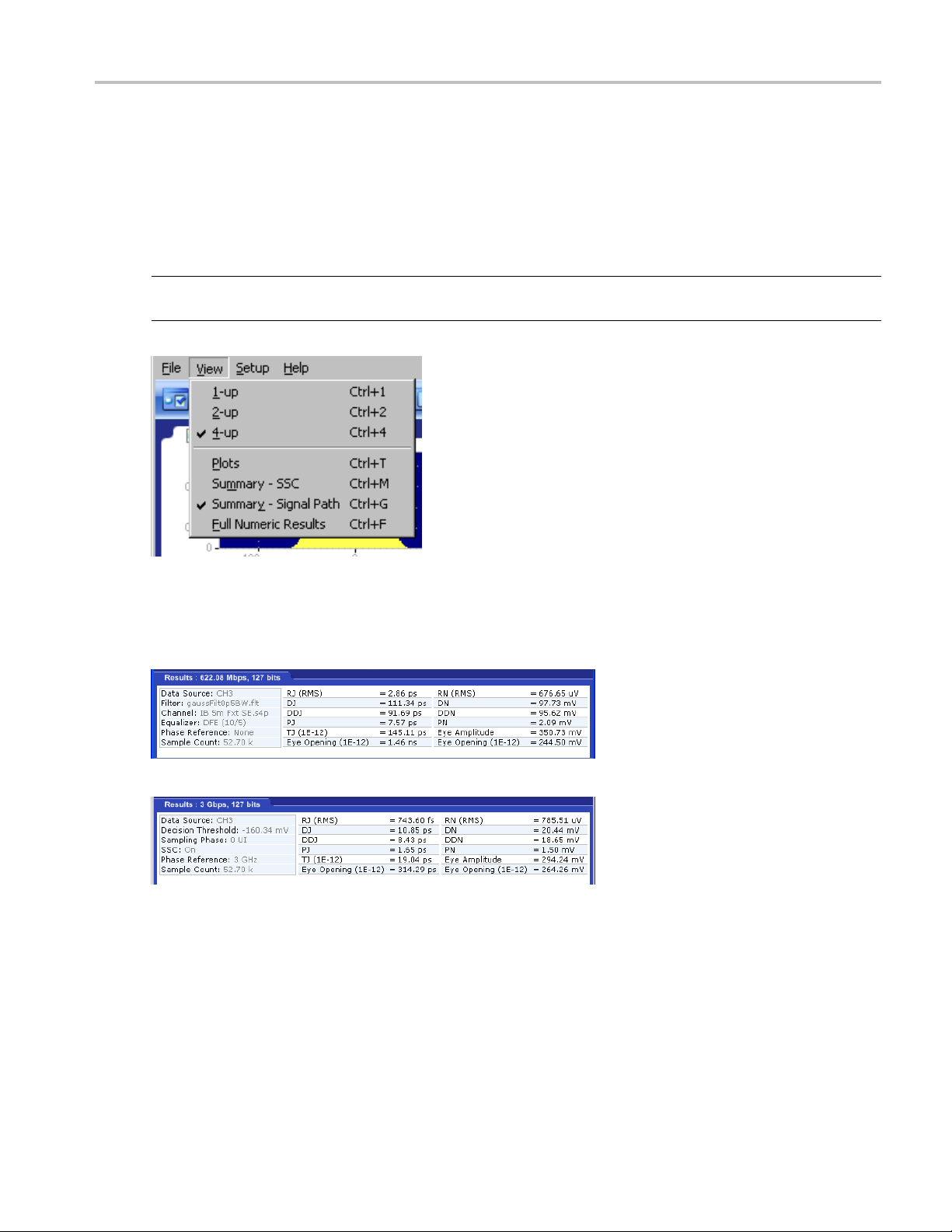
Operating Basics Working with Numeric Results
Working with Numeric Results
After an analysis is complete, you can display the results as numeric data in either a summary or detailed
(full) table. Use the View menu in the file menu bar to select how to display the data. A summary of data
allows room t
TIP. Using a second monitor (connected to the TekScope) to display the 80SJNB application allows the
numeric results display to show all results at once.
o display the plots while the full results replaces the plot display entirely.
There are two views of the summary table: SSC and Signal Path. Both summary selections contain the
noise and jitter measurements but not the breakdown of the measurements. The two summaries differ by
displaying relevant application settings.
The detailed table (when selected) expands to fill the entire screen, removing any plot displays.
80SJNB Printable Online Help 61

Operating Basics Working with Numeric Results
You can easily switch between summary and detailed numeric displays by clicking the numeric results
button
To hide the summary table and provide more room for the plot displays, click the numeric data table tab.
Click the tab again to show the summary data table.
Here you can see that the plot windows fill the entire screen and the tab for the numeric details is showing
at the bottom of the screen.
and the plot window buttons .
62 80SJNB Printable Online Help

Operating Basics An Application Example
See Also:
Working with Plots (see page 50)
Noise Measurement Definitions (see page 46)
Jitter Measurement Definitions (see page 45)
Dual Dirac M
SSC Modulation Measurement Definitions (see page 46)
easurement Definitions
An Application Example
The following example uses the 80SJNB application on an optical signal for fast analysis of BER, Jitter,
and Noise. This simplified application example shows how to configure and use the application. This may
help you
Requirements:
when setting up your own test situation.
DSA8300 oscilloscope
80SJNB software
ADVTRIG Advanced Trigger Option installed
Optical module with clock recovery. The following example uses the 80C11-CR4 Optical Sampling
Module.
SMA cables
(see page 45)
Set Up the Oscilloscope
1. Install the modules and make the signal connections (the example assumes using channel 1 as the
signal source).
2. Turn on the instrument and wait for instrument and application startup to complete.
3. Push the Default Setup front panel button.
elect Channel 1.
4.S
5. Push the SETUP DIALOGS button.
6. Click the Horz tab.
7. Set the Horizontal scale to 5ns.
8. Click the Mode/Trigger tab.
80SJNB Printable Online Help 63

Operating Basics An Application Example
9. Verify that Trigger Source is set to Clock and select C1 Clock Recovery as the clock source .
10. Click th
11. Click the Pattern Sync/FrameScan Setup button.
12. Enter the Data Rate parameter (for example, 9.8 Gbps).
13. Set the Pattern Length parameter (for example, 127 bits).
e Pattern button in the Scope Mode (Clock Trigger Source) area.
14. Click Close.
64 80SJNB Printable Online Help
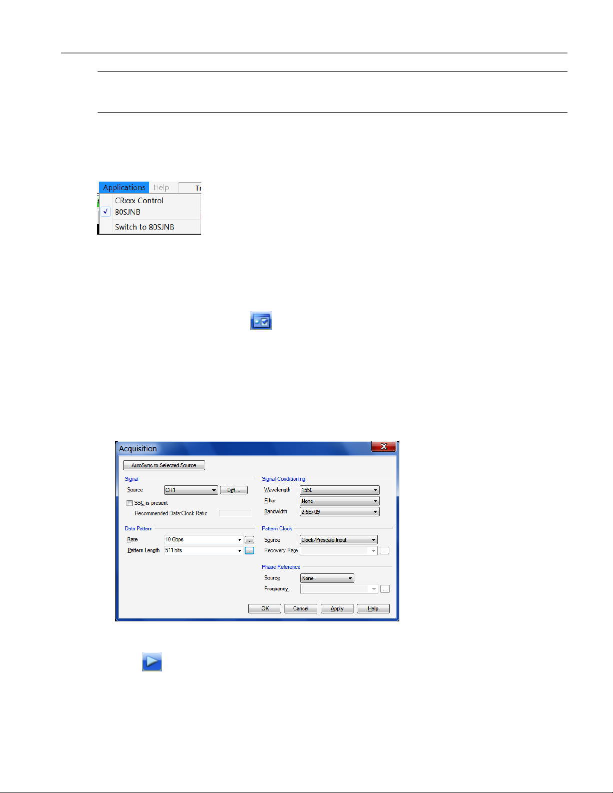
Operating Basics An Application Example
NOTE. You should now have a stable signal display on the DSA8300. If not, recheck all settings, signal
source, and connections. The 80SJNB application requires a stable signal to acquire data for accurate
measurements
.
Set Up the 80SJNB Application
1. Click Applications > 80SJNB in the DSA8300 menu to start the 80SJNB application.
You can also use the Windows 80SJNB desktop shortcut or the Windows Start menu Start > Programs >
Tektroni
1. Wait for the 80SJNB application to finish loading.
x Applications > 80SJNB > 80SJNB to start the 80SJNB application.
2. Click the Acquisition button (
3. Most of the configuration settings are already filled in, as the 80SJNB application acquired the values
from the oscilloscope configuration. If not, click the AutoSync to Selected Waveform button to sync
the Source, Data Pattern, and Pattern Sync settings to the oscilloscope.
Since this is an optical signal and we’re using the clock recovery signal, you’ll need to select the
optical signal filter and select the clock recovery settings.
The setup in this example does not include a Phase Reference module, so set this to None.
) to open the acquisition dialog box.
Click OK to apply the settings and close the dialog box.
4. Click
80SJNB Printable Online Help 65
to start the acquisition and processing cycle.

Operating Basics An Application Example
While the cycle is running, you’ll see the sequence of events displayed at the bottom of the application
display. When the cycle is complete, the application displays the message “Analysis Complete.”
5. Once the cycle is complete, you’ll see the displayed results. The example below shows a four plot
display with the summary table of the numerical results.
Working with the Results
1. Click to minimize the plot displays and show the detailed results table.
2. Redisplay the plot (or plots) by selecting one of the plot display buttons .
66 80SJNB Printable Online Help

Operating Basics An Application Example
Click the Results tab to minimize the detailed list to a summary list.
3. With the plots now redisplayed, click the Configure Plot icon ( ) on the plot tab to display a
drop-down menu for that plot. The menu provides several functions, one of which is to select a
different type of plot to display in that window.
You c an
last processing cycle.
4. To f u r
tool
The plot opens in a new window to provide further data analysis and visualization of the plot displays.
MATLAB provides multiple capabilities to display and annotate the plot diagrams, including:
The following figure shows a 3D BER Eye plot using the rotate function.
select any plot type. The plot is displayed based on the data based on the results of the
ther examine a plot, you can display any plot in a MATLAB window, providing you with more
s to work with the data. Click the Configure Plot (
Pan and Zoom
2D and 3D visualization
Rotation
ta Cursors
Da
Color enhancements
) icon and choose Examine.
80SJNB Printable Online Help 67

Operating Basics An Application Example
Close the window to return to the 80SJNB d isplay.
This is the end of the example. You can continue on by acquiring new data, displaying various types of
plots, and examine the plots with the various tools available.
68 80SJNB Printable Online Help

Parameters About Application Parameters
About Application Parameters
These topics list the 80SJNB application parameters and include the menu default settings. The parameter
tables list the selections and startup values for each option.
Analysis Settings
Acquisition Settings (see page 70)
Signal Path Settings (see page 71)
Refer to the GPIB topics for a list of the GPIB Command Syntax with the arguments, variables, and
variable values that correspond to the 80SJNB parameters.
You should refer to the documentation for your TekScope for operating details of the oscilloscope controls.
See Also:
GPIB Reference Materials (see page 73)
Analysis Settings
This table lists the default values of the Analysis settings when the 80SJNB application is first started. If
you change these settings, they remain in effect for all successive sessions of the application.
Control Startup settings
od
Meth
sion Threshold
Deci
eUnit
Tim
Sampling Phase
asurement BER
Me
xxx
(see page 69)
Spectral + BUJ
Normalized: 50%
Seconds
it Intervals: 0 UI
Un
00E-12
1.
80SJNB Printable Online Help 69

Parameters Acquisition Settings
Acquisition Settings
This table lists the default status of the Acquisition settings when the 80SJNB application is first started. If
you change these settings, they remain in effect for all successive sessions of the application.
Control Startup settings
Signal
Source
SSC is present Checked
Difference Waveform
Positive First valid input channel
Negative blank
Data Pattern
Rate
Pattern Length
Signal Conditioning
Wavelength None
Filter None
Bandwidth blank
Pattern C lock
Source CLOCK INPUT/PRESCALE TRIGGER front panel
Recovery Rate blank
Phase Reference
Source
Frequency blank
xx
x
First valid input channel
User defined
User defined
connector
None
70 80SJNB Printable Online Help

Parameters Signal Path Settings
Signal Path Settings
This table lists the d efault status of the Signal Path settings when the 80SJNB application is first started. If
you change these settings, they remain in effect for all successive sessions of the application.
Control Startup settings
Filter
Uncorrelated Scaling
Channel
Data Type Frequency Domain
Uncorrelated Scaling
Equalizer
Taps
FFE Taps 1
FFE Taps/Symbol
DFE Taps 0
Filter
FFE Reference Tap
Uncorrelated Scaling
Rise Time Selector
User Rise Time (ps)
xxx
1.00
1.00
1
1
1.00
Track Data Rate
200
80SJNB Printable Online Help 71

Parameters Signal Path Settings
72 80SJNB Printable Online Help

Remote Control Remote Control Introduction
Remote Control Introduction
The 80SJNB software application can be controlled programmatically through the programmatic interface
of the sampling oscilloscope on which it is running. Communication with the application is accomplished
using VARIAB
Your program should comply with the following guidelines:
The application startup must complete before sending additional GPIB commands to the a pplication.
Querying the variable “Application” returns “80SJNB” when the application startup is complete.
The measurements cycle must complete be fore you query data. Que rying the variable DataReady
returns “True” when the data is ready.
Because the oscilloscope software hosts the GPIB interface for the 80SJNB application, there is some
additional information that is helpful for successful programming.
See Also:
LE:VALUE remote GPIB commands.
GPIB Re
Programming Tips (see page 74)
Variable:Value Commands (see page 75)
Results Queries (see page 82)
Programming Examples (see page 84)
ference Materials
(see page 73)
GPIB Reference Materials
To use G PIB commands with your TekScope, you can refer to the following materials:
e Programming Examples
Th
The online Programmer Guide for the TekScope.
See Also:
tarting and Setting Up the Application Using GPIB
S
(see page 84) topic for guidelines to use while designing a GPIB program.
(see page 73)
80SJNB Printable Online Help 73

Remote Control Programming Tips
Programming Tips
How the Variab
Programmable Interface (PI) commands for the 80SJNB software package (JNB) are implemented using
avariable/v
(variable:value “VariableName”,”VariableValue”) or queried (variable:value? “VariableName”) from the
PI. When a set command is received, if the variable does not already exist in the table, it is created and the
specified value is associated with that variable. If the variable is already in the table, the specified value
will replace the existing value. There is no checking done by the table on variable names or values. Since
both items are strings, any arbitrary pair of strings can be associated with each other in this table.
le Value Table Works
alue table. This table associates named variables with text values. These values can be set
Polling and Limit of Variable Values
Each tim
application polls the oscilloscope software application every 200 ms to see if an event occurred. If so, JNB
queries for the event information which tells JNB which va riable changed and the new value. JNB parses
this information to find the variables pertinent to its operation and reads the new values for those variables.
These new values can change the state of JNB (for example selecting a new data source channel) or can
cause JNB to perform an operation (for example, setting “SequencerMode” to “Run”).
Because JNB polls for changes at a fixed rate, the oscilloscope application might indicate that a list of
variables has changed since the last time JNB polled for changes. There are two consequences of this
oper
e a change is made to a variable’s value in the table, an event is generated. The 80SJNB software
ation.
First, when JNB receives a list of changes, it does not necessarily execute those changes in the order in
ch they were sent to the o scilloscope from the PI. This means that sending a c ommand to change
whi
the data source (for example, “DataSource”,”C1”) followed immediately by starting sequencing
(“SequencerState”,”Run”) does not guarantee that the source channel is changed before JNB begins
the sequencing operation. To be sure of proper execution order of these commands, a delay of at least
400 ms should b e inserted before starting certain JNB operations.
Commands that should be preceded by a delay include:
“SequencerState”,”Run”
“ExportCurve”,”GO”
“SaveRecallData”,”Save”
“SaveRecallData”,”Recall”
“Setup”,”Save”
“Setup”,”Recall”
Second, there is a limit of 15 variable/value table changes that can be reported for any one polling
event. If more than 15 changes have occurred between JNB polls of the oscilloscope software, the
later changes will not be seen by JNB so it will not respond to those commands.
74 80SJNB Printable Online Help

Remote Control Syntax
How the Variable Value Table Is Updated
JNB only updates table entries when it has new data to report. For example, if an error occurs during
sequencing, the variables “ErrorCode” and “ErrorMessage” are updated by JNB with the appropriate
values. However, JNB will only update those variables if another error occurs. If a subsequent sequence is
run without e
The user program must be written to explicitly clear these variables, setting the variables to null strings
(“”) before starting a new seque nce.
Variables that should be set to null strings (“”) before starting a sequence operation include:
ErrorCode
ErrorMessage
DataReady
rrors, the “ErrorCode” and “ErrorMessage” variables will continue to report the old values.
Determi
The “Application” variable shows whether 80SJNB is running or not. When it is running, this variable is
set to “
error and exits abnormally, it will not set the “Application” variable to “Done”, leaving the variable set
to “80SJNB”. In this circumstance, it is not possible to use this variable to determine if JNB is running.
One way to reliably determine if JNB is running is to set the “PatternLength” variable to “1”. If JNB is
running, it will set this variable to “2” since 2 is the minimum allowable value for “PatternLength”. If JNB
is not running, the variable value will remain at “1”. Be sure to wait at least 400 ms after setting the value
to “1
Syntax
The VARIABLE:VALUE command accepts string a rguments for a control o r data variable and a value
to which to set the argument.
To set a variable to a value:
VARIABLE:VALUE "<VariableName>","<VariableValue>"
NOTE. The arguments <variable name> and <variable value> are required in the order indicated with no
spaces allowed.
ning If 80SJNB Is Running
80SJNB”. When JNB exits normally, the variable is set to “Done”. However, if JNB encounters an
” before querying the status of this variable.
To query the value in a variable:
VARIABLE:VALUE? <variable name>
NOTE. Commands are case and space sensitive. Your program will not operate correctly if you do not
follow the capitalization and spacing precisely.
80SJNB Printable Online Help 75

Remote Control Arguments and Queries
See Also:
Variable:Value Command Arguments and Queries (see page 76)
GPIB Commands Error Codes (see page 84)
Programming Examples (see page 84)
Arguments and Queries
Name Value Fun ction Query form returns
AnalysisMethod
Application Exit Exits the application Done
Bandwidth Any valid bandwidth as
BER
CeActive {True | False}
CeDomain Time | Frequency Sets the domain in which
CeFdSParametersFile Full path name of a file
CeFd2PortMatrixSelector {11 | 12 | 21 | 22} Selects an S-parameter
CeFd4PortDataType {SingleEnded | Differential} Selects the type of data
CeFd4PortLayout {DC21 | CD21 | 12DC |
CeFd4PortMapping Any permutation of 1234
CeTdReferenceFile Full path name of a file
{CDF | Spectral} Sets the jitter and noise
analysis method. Spectral
is legacy. Default is CDF
(Cumulative Distribution
Function)
Sets or returns the
defined by the selected
source module
Any valid floating point
value between 1e-3 and
1e-24 inclusive
name
12CD}
(for example, 1234, 1324
or 2143)
name
bandwidth in Hertz for
use when Filter is set to
None
Sets or returns the current
BER value
Activates or deactivates
the channel emulator
the channel characteristics
are defined
Defines the channel’s
S-parameter
when using a 2-port
Touchstone file
when using a 4-port
Touchstone file
Sets the data arrangement
used by a 4-port
Touchstone file containing
Differential data
Sets the port mapping used
by a 4-port Touchstone file
containing SingleEnded
data
Defines the time domain
reference waveform
Current value
Current value
Current value
True, False
Current value
Current value
Current value
Current value
Current value
Current value
Current value
76 80SJNB Printable Online Help

Remote Control Arguments and Queries
Name Value Function Query form retu
CeTdTransmis
CeUncorrelatedScaling
ClockRecov
ClockSou
DataRat
DataReady
aSource
Dat
DecisionThresholdAbs
DecisionThresholdPct
sionFile
eryRate
rce
e
Full path name
name
Any number in t
0.01-100.0
Valid values include any
communicat
token for communication
standards supported by
the clock r
or a positive floating point
value if the clock recovery
unit supp
{ClockPr
C1ClockRecovery |
C1CRClockPrescale
|C3Cloc
C3CRClockPrescale}
Any vali
floating point value or
communication standard
{True | False} Sets or r eturns a value
1 | CH2 | CH3 | CH4 |
{CH
CH5 | CH6 | CH7 | CH8 |
MATH1 | MATH2 | MATH3 |
H4 | MATH5 | MATH6
MAT
| MATH7 | MATH8 | <file
name >}
Any valid floating point
lue
va
ny valid floating point
A
value between 0.0 and
1.0 inclusive
of a file
he range
ion standard
ecovery module
orts user rates
escale |
kRecovery |
d positive
Defines the tim
transmission waveform
Sets the Channel
uncorrelated scaling factor
Overall sign
uncorrelated scaling factor
is a product of all active
uncorrelat
Sets or retu
recovery rate
Sets or re
source
Sets or returns the
expected data r ate
ating if sequencing is
indic
complete and data is ready
to be read
ng this value to
Setti
False before beginning
a sequence prevents
dentally reading the
acci
DataReady value from a
previous sequence before
reset by the application
it is
s or returns the data
Set
source
Math expressions must
rogrammed through
be p
the oscilloscope GPIB
interface commands
Sets or returns the absolute
cision threshold value
de
ets or returns the
S
normalized decision
threshold value
e domain
al path
ed scaling values
rns the clock
turns the clock
Current value
Current value
Current val
Current v
Communication standard
or current value
True, False
Cur
file name is the name of the
file recalled
Current value
urrent value
C
ue
alue
rent value
rns
80SJNB Printable Online Help 77

Remote Control Arguments and Queries
Name Value Fun ctio n Query form retu
DecisionThresholdUnits
{Absolute, No
rmalized}
Sets or return
s the desired
Current value
decision threshold value to
use
By setting the
units
to Absolute, the
DecisionThresholdAbs
value is used
. If the units
are set to Normalized,
the decision threshold
is calculat
ed based on
waveform data according to
the DecisionThresholdPct
d value.
True or False
EqActive
{True | Fal
se}
normalize
Activates or deactivate the
equalizer
EqAutosetTaps
{Run}
Automatically computes
the equal
ization
Current v
Error
alue or Done,
coefficients
SpCompute must be run
first
EqDFETaps An integer in the range
1-40
EqDFETapCoefficient<n>
where <n> is in the range
Any numb
-100.0 to +100.0
er in the range
Sets the
number of DFE
taps
Sets the value of a DFE tap
coefficient
value
Current
Current value
1–40
aultDFETaps
EqDef
EqDefaultFFETaps
EqFFEReferenceTap
2
{Run} Sets t
he DFE taps to
default values
2
{Run} Sets the FFE taps to default
values
An integer in the range 1 –
EqFFETaps
Selects the F FE reference
tap
nt value or Done,
Curre
Error
Current value or Done,
Error
Current value
EqFFEReferenceTap-1 must be an integer
ssibly 0) multiple of
(po
EqFFETapsPerSymbol
FETaps
EqF
EqFFETapsPerSymbol One of 1, 2, 5, 10 but not
nteger in the range
An i
1-100
arger then EqFFETaps
l
Sets the number of FFE
taps
Sets the number of FFE
aps per symbol or unit
t
Current value
Current value
interval
EqFFETapCoefficient<n>
where <n> is in the range
A
-100.0 to +100.0
Sets the value of an FFE
tap coefficient
Current value
ny number in the range
1–100
EqLoadTaps
2
{Run}
EqRiseTimeSelector {DataRate | TapInterval |
User}
Loads the equalizer
configuration from a file
Defines how the equalizer
rise time is determined
Current value or Done,
Error
Current value
rns
78 80SJNB Printable Online Help

Remote Control Arguments and Queries
Name Value Function Query form retu
EqSaveTaps
EqTapsFilena
2
me
{Run} Saves the equa
configuration to a file
Full path name of a file Sets the file used
lizer
Current value
Error
Current value
or Done,
for EqLoadTaps and
EqSaveTaps
EqUncorrel
atedScaling
Any number in the range
0.01-100.0
Sets the Equ
alizer
uncorrelated scaling factor
Current val
ue
Overall signal path
uncorrelat
ed scaling factor
is a product of all active
uncorrelated scaling values
EqUserRiseTime An integer in the range
1-4000
When EqRiseTimeSelector
is set to U
ser, this defines
Current value
the rise time in picoseconds
ErrorCode
Returns a
numeric code
Current value
corresponding to the last
error or 0 if no error
ErrorMessage Returns the last error
Current value
message
ExportCurve
23
{GO} Sets or returns the export
action
Current value or Done,
Error
Error is returned if export is
unsuccessful
,MAT}
1
Sets the file name used
xporting data
when e
or returns the current
Sets
Curr
ent value
ExportFilename
ExportFormat
<file name >
{CSV
plot diagram export format
rtType
Expo
ACQWFM | CORRWFM,
RJPDF | PJPDF |
JPDF | RJPJSPEC
RJP
Sets or returns the type of
export to perform
Current value
| DDJPDF | DJPDF |
DDJSPEC | TJPDF |
|HBATH|QHBATH
DDJ
| RNPDF | PNPDF |
RNPNPDF | RNPNSPEC
DNPDF | DNPDF |
|D
DDNSPEC | TNPDF |
DDN | VBATH | QVBATH
EREYE | QEYE |
|B
PDFEYE | CORREYE
| BERCONTOUR |
PCHANPDFEYE
S
| SPCHANWFM
| SPFILTWFM |
PFILTPDFEYE
S
| SPINPDFEYE |
SPINWFM | SPEQWFM |
SSCPROFILE
rns
80SJNB Printable Online Help 79

Remote Control Arguments and Queries
Name Value Fun ctio n Query form retu
FiActive
{True | False}
Activates or deactivates
True, False
the filter
FiFilename
Full path name
of a file
Defines the filt
er file
Current value
name
FiUncorrelatedScaling
Any number in
0.01-100.0
the range
Sets the Filter uncorrelated
scaling factor
Overall sig
nal path
Current value
uncorrelated scaling factor
is a product of all active
ed scaling values
urns the
ength in bits
ired with a phase
Current va
lue
Current value
True, False
Filter Any valid communication
standard a
sdefined by the
selected source module
PatternLength Any integer value between
2 and 100,000
PhaseRe
ferenceEnabled
uncorrelat
Sets or ret
communication standard of
the source
Sets or returns the data
pattern l
Indicates whether the data
was acqu
reference unit active or
not for both acquired and
d data
recalle
eferenceFrequency
PhaseR
id phase reference
Any val
frequency as defined by the
returns the phase
Sets or
reference frequency
Curren
t value
selected phase reference
e module
sourc
ReferenceSource
Phase
-or- C1_C2,
{C1C2
C3C4 -or- C3_C4,
r returns the phase
Sets o
reference source module
Curre
nt value
C5C6 -or- C5_C6,
-or- C7_C8}
C7C8
RecallDataFilename
<file
name >
1
ifies the name of the
Spec
file when recalling a saved
data file
RecallFilename
mplingPhase
Sa
<file name >
yvalidfloating point
An
value between –0.5 and
+0.5 inclusive
SamplingPhaseAbs Any valid floating point
alue
v
1
Sets the name of the file
n recalling a setup
whe
ts or returns the
Se
rrent value
Cu
normalized sampling
point value
Sets or returns the absolute
ampling point value
s
Current value
rns
80 80SJNB Printable Online Help

Remote Control Arguments and Queries
Name Value Function Query form retu
SamplingPhas
eUnits
{Absolute, No
rmalized}
Sets or return
s the desired
Current value
sampling point value to
use.
If the units ar
eset
to Absolute, the
SamplingPhaseAbs value
is used. If th
e units
are set to Normalized,
the sampling point is
calculated
based on
waveform data according
to the SamplingPhase
d value.
e name used
SaveDataF
ilename
<file name >
normalize
1
Sets the fil
when saving data files
SaveFilename <file name >
1
Sets the file name used
when saving setup files
SaveRecallData
3
{Save, Recall} Save saves the a cquired
datatot
he file name
specified by the command
Done, Error
Error is returned if
unsucce
ssful
SaveDataFilename
recalls the acquired
Recall
data from the file name
specified by the command
DataFilename
Recall
ncerMode
Seque
SequencerState
leSequence,
{Sing
FreeRun}
3
{Run | Pause | Stop} Sets or returns the
he sequencer mode
Sets t
Startup default is Free Run
ncer mode
Seque
Sequencer state
Measurement Sequencing
e Stop Sequencing
or th
command
Setup
3
{Recall | Save | Default} Performs the
Save/Recall/Default setup
ion
act
Current value or Done,
Error
or is returned if
Err
unsuccessful
SpCompute
2
{Run}
computes results with
Re
the latest Signal Path
Current value or Done,
Error
definition on the acquired
ta
da
SC
S
True | False}
{
elects whether SSC is
S
urrent value
C
present in the signal
Setting to True requires a
hase reference module to
p
be installed and configured
rns
80SJNB Printable Online Help 81

Remote Control Variable:Value Results Queries
Name Value Fun ctio n Query form retu
TimeUnits
{S | UI} Sets or return
Wlength Any valid wave
defined by the selected
source module
xxx
1
<file name > is a string of 1 to 40 characters that are valid for file names according to the Windows file system standards.
2
After running the default setup command, this argument is not initialized and a query returns an empty string "".
3
Command should be preceded by a delay of at least 400 ms.
Variable:Value Results Queries
These values, when used with the Variable:Value command, return the results for the individual
measurement results.
Value Function
BUJDD Returns the Bounded Uncorrelated Jitter
BUNDD Returns the Bounded Uncorrelated noise.
DCD abc Returns the Duty Cycle Distortion.
DDJ Returns the Data Dependent Jitter.
DDN Returns the Data Dependent Noise.
DDN0 Returns the Data Dependent Noise on logical level 0.
DDN1 Returns the Data Dependent Noise on logical level 1.
DDPWS Returns the measured Data Dependent Pulse Width Shrinkage.
DJ Returns the measured deterministic jitter.
DJDD Returns the Deterministic Jitter computed in the Dual Dirac model.
DN Returns the measured deterministic noise.
EA
EOH Returns the Horizontal Eye Opening at user specified BER.
EOV Returns the Eye Opening at user-specified BER.
NPJDD Returns non periodic jitter
NPNDD Returns non periodic noise
PJ
PJH
PJV
PN Returns the measured periodic noise.
PNH
PNV
Returns the amplitude of the eye computed as the mean-to-mean of logical 1 and
logical 0 bit levels sampled at the user defined Sampling Phase.
Returns the measured Periodic Jitter (peak-to-peak).
Returns the Horizontal component of periodic jitter (peak-to-peak).
Returns the Vertical component of periodic jitter (peak-to-peak) induced by noise
converted to jitter through an average slew rate.
Returns the Horizontal component of periodic noise (peak-to-peak) induced by jitter
converted to noise through an average slew rate.
Returns the Vertical component of periodic noise (peak-to-peak).
length as
s the units for
the time scale
Sets or returns the
wavelength of the sources
rns
S, UI
Current value
82 80SJNB Printable Online Help

Remote Control Variable:Value Results Queries
Value Function
RJ
RJH
RJV
RJDD Returns the Random Jitter computed in the Dual Dirac model.
RN Returns the measured Random Noise.
RNV
RNH
TJ
TN
SSCfreq Returns the spread spectrum clock modulation frequency.
SSCmag
xxx
Returns the measured random jitter (RMS).
Returns the Horizontal component of random jitter (RMS).
Returns the Vertical component of random jitter induced by noise converted to jitter
through an av
erage slew rate (RMS).
Returns the Vertical component of random noise.
Returns the Horizontal component of random noise induced by jitter converted to
noise through an average slew rate.
Returns the To tal Jitter at user-specified BER.
Returns the Total Noise at user-specified BER.
Returns the spread spectrum clock modulation magnitude.
80SJNB Printable Online Help 83

Remote Control GPIB Commands Error Codes
GPIB Commands Error Codes
Error code Description
–1 Read error message, no error code available
NOTE. If an error code of –1 is returned, use the Error M essage query for error
condition details.
1 The channel does not support bandwidth
2
3 No data to export
4 Not allowed to change setting while sequencing
5
6 Argument cannot be null
7
8
9
10 No data source selected
11
12
13 The pattern is not synchronized or is too small
14
15
16
17
18
19
20
21
22 The channel does not support wavelength
23
24
25
26
27
28
xxx
Phase characterization failed
Invalid value
Value is outside the range of acceptable values
Query curve returned no data
Unexpected GPIB response
One or more WfmDBs are on; turn them off to continue
Trigger failure, check your configuration
Cannot export the curve
Could not analyze edge
Histogram testing is on; turn it off to continue
Mask testing is on; turn it off to continue
One or more measurements are on; turn them off to continue
Waveforms other than 80SJNB signal source are on; turn them off to continue
Save setup failed
Recall setup failed
Curve has multiple components
A Mag View is on; turn it off to continue
SSC activation failed; phase reference module required
SSC activation failed; setup phase reference module
Save data failed
Recall data failed
Programming Examples Introduction
An example of communicating with the 80SJNB application using VARIABLE:VALUE remote GPIB
commands is to simply start the application by sending the following command:
84 80SJNB Printable Online Help

Remote Control Program Example: Configure and Operate 80SJNB
APPlication:ACTivate "80SJNB"
A more extensive program example steps you through the following actions:
1. Starting the application.
2. Configuration and setting analysis state variables.
3. Starting and checking the state of the acquisition and processing cycle.
4. Check for errors.
5. Query measurement results.
6. Export data.
Program Examples:
Configure and Operate the 80SJNB (see page 85)
Measuring Jitter in Presence of SSC (see page 87)
Compensating for Signal Path Impairments with Equalization (see page 89)
See Also:
About the GPIB Program and Guidelines (see page 73)
GPIB Reference Materials (see page 73)
Variable:Value Command (see page 75)
Results Queries (see page 82)
Program Example: Configure and Operate 80SJNB
The following sequence of commands shows the GPIB commands used to configure and operate the
80SJNB jitter analysis application. All commands are sent to the instrument which hosts the programmable
interface for the 80SJNB.
NOTE. The examples presume that you are familiar with designing GPIB programs.
All words within quotes are case sensitive and must be entered exactly as shown, including spaces and
quotes.
1. Send the command to start the 80SJNB application.
APPLICATION:ACTIVATE "80SJNB"
2. Set the signal source channel, data rate, and pattern length to be analyzed.
80SJNB Printable Online Help 85

Remote Control Program Example: Configure and Operate 80SJNB
VARIABLE:VALUE "DataSource","CH1"
VARIABLE:VALUE "DataRate","10.3125e9"
VARIABLE:VALUE "PatternLength","32767"
3. Set the following variables before starting the analysis. The application updates these v alues to signal
the application’s analysis state.
VARIABLE:VALUE "DataReady","False"
VARIABLE:VALUE "ErrorCode",""
4. Start the acquisition and processing cycle.
VARIABLE:VALUE "SequencerState","Run"
5. Check the state of the acquisition and processing cycle.
Query the following variables:
VARIABLE:VALUE? "DataReady"
VARIABLE:VALUE? "SequencerState"
Loop until DataReady is True or SequencerState is Stop.
6. Check to see if there were errors.
VARIABLE:VALUE? "ErrorCode"
If the response for ErrorCode is not 0 then an error has occurred. Query
VARIABLE:VALUE? "ErrorMessage"
to retrieve the error message.
7. If the DataReady variable is set to True (queried in step 5), you can query for measurement results.
For example to query the deterministic jitter:
VARIABLE:VALUE? "DJ"
8. You can also export the plot data. The following commands set the format, data to export, file name,
and then exports the data.
VARIABLE:VALUE "ExportFormat","CSV"
VARIABLE:VALUE "Ex
VARIABLE:VALUE "ExportFilename","C:\Users\<username>\Documents\
myDJPDF.csv"
VARIABLE:VALUE "ExportCurve","GO"
portType","DJPDF"
9. Query the ExportCurve variable to determine when the data export has completed:
VARIABLE:VALUE? "ExportCurve"
The application sets the ExportCurve value to "Done" when the data is exported.
86 80SJNB Printable Online Help

Remote Control Program Example: Measuring Jitter in Presence of SSC
Program Examples:
Measuring Jitter in Presence of SSC (see page 87)
Compensating for Signal Path Impairments with Equalization (see page 89)
Program Example: Measuring Jitter in Presence of SSC
The following instruction sequence shows jitter analysis in the presence of SSC and the measurement of
the SSC characteristics.
NOTE. The examples presume that you are familiar with designing GPIB programs.
All words within quotes are case sensitive and must be entered exactly as shown, including spaces and
quotes.
NOTE. The measurement system configuration should include a correctly set up and configured Tektronix
BERTScope CR series instrument (clock recovery instrume nt, or CRI) that supports SSC.
An 82A04 Phase Reference module is required for measuring signals that contain SSC.
1. Send the command to start the 80SJNB application.
APPLICATION:ACTIVATE "80SJNB"
2. Set the signa l source channel, data rate, pattern length, and data-to-clock ratio
VARIABLE:VALUE "DataSource","CH1"
VARIABLE:VALUE "DataRate","3e9"
VARIABLE:VAL
UE "PatternLength","127"
3. Initialize analysis state and error code.
VARIABLE:VALUE "DataReady","False"
VARIABLE:VALUE "ErrorCode",""
4. Tell 80SJNB to look for SSC.
VARIABLE:VALUE “SSC”,”True”
5. Set up the phase reference module source and frequency since it is required for SSC analysis
VARIABLE:VALUE “PhaseReferenceSource”,”C7_C8”
VARIABLE:VALUE “PhaseReferenceFrequency”,
”3e9”
6. Set up the BERTScope clock recovery unit that supports SSC. Set clock frequency to 3e9. Refer to the
documentation for the BERTScope for more details.
80SJNB Printable Online Help 87

Remote Control Program Example: Measuring Jitter in Presence of SSC
The following table lists recommended settings:
Recommended
Clock recovery
Data rate ran g
500 Mbps – 1 Gbp
1 Gbps – 2 Gbps Data Rate * 2 Standard
2 Gbps – 4 Gbp
4 Gbps – 8 Gbp
8 Gbps – 12.
xxx
e
s
s
5 Gbps
frequency (CR
s
Data Rate * 4 Standard
Data Rate
Data Rate
Data Rate
I)
Clock recovery
output rate (C
Standard
Subrate (1/
Subrate (1
/4)
Data:Clock ratio
RI)
2)
(JNB)
1:4
1:2
1:1 Data Rate
2:1
4:1
Phase reference
frequency (JN
Data Rate * 4
Data Rate * 2
Data Rate/2
Data Rate/
B)
4
7. Clear the error code to prepare for starting the application.
VARIABLE:VALUE "Err
orCode",""
8. Start the acquisition and processing cycle.
VARIABLE:VALUE "SequencerState","Run"
9. Check the state of the acquisition and processing cycl
VARIABLE:VALUE? "DataReady"
VARIABLE:VALUE? "SequencerState"
e. Query the following variables:
Loop until DataRead is True or SequencerState is Stop.
10. Check if there were errors:
VARIABLE:VALUE? “ErrorCode”
If the response for ErrorCode is not 0, then an error has occurred. Query:
VARIABLE:VALUE? “ErrorMessage”
11. If the DataReady variable is set to True, and no errors have occurred, you can query for measurement
results.
For example to query the periodic jitter and total jitter:
VARIABLE:VALUE? “PJ”
VARIABLE:VALUE? “TJ”
12. Query for SSC measurements, magnitude and frequency.
VARIABLE:VALUE? “SSCmag”
VARIABLE:VALUE? “SSCfreq”
13. You can also export the SSC profile. The following commands set the format, data to export, file
name, and then export the data.
VARIABLE:VALUE "ExportFormat","CSV"
VARIABLE:VALUE "ExportType"," SSCPRO FILE "
88 80SJNB Printable Online Help

Remote Control Program Example: Compensating for Signal Path Impairments with Equalization
VARIABLE:VALUE "ExportFilename","C:\Users\<username>\Documents\
mySSCprofile.csv"
VARIABLE:VALUE "ExportCurve","GO"
14. Query the ExportCurve variable to determine when the data export has completed.
VARIABLE:VALUE? "ExportCurve"
The application sets the ExportCurve value to "Done" when the data is exported.
Program Examples:
Configure and Operate the 80SJNB (see page 85)
Compensating for Signal Path Impairments with Equalization (see page 89)
Program Example: Compensating for Signal Path Impairments with
Equalization
The following programming example shows a sequence of commands that configures the Signal Path with
a Channel emulator that causes severe ISI. Then an Equalizer is inserted and configured to compensate
for the effects of the ISI and assess the results of equalization by measuring data dependent jitter and
vertical eye opening.
NOTE. The examples presume that you are familiar with designing GPIB programs.
All words within quotes are case sensitive and must be entered exactly as shown, including spaces and
quotes.
NOTE. The 80SJNB Advanced option must be enabled. The S-parameter file is available from examples,
Sdd21.s1p, located in My Documents.
1. Send the command to start the 80SJNB application.
APPLICATION:ACTIVATE "80SJNB"
2. Set the signal source channel, data rate, pattern length, and data-to-clock ratio.
VARIABLE:VALUE "DataSource","CH1"
VARIABLE:VALUE "DataRate","9.95328e9"
VARIABLE:VALUE "PatternLength","127"
3. Initialize the analysis state and error code.
VARIABLE:VALUE "DataReady","False"
80SJNB Printable Online Help 89

Remote Control Program Example: Compensating for Signal Path Impairments with Equalization
VARIABLE:VALUE "ErrorCode",""
4. Start the acquisition and processing cycle.
VARIABLE:VALUE “SequencerState”,”Run”
5. Check the state of the acquisition and processing cycle.
Query the fo
VARIABLE:VALUE? "DataReady"
VARIABLE:VALUE? "SequencerState"
llowing variables:
Loop until DataRead is True or SequencerState is Stop.
6. Check if there were errors.
VARIABLE:VALUE? “ErrorCode”
If the re
VARIABLE:VALUE? “ErrorMessage”
sponse for ErrorCode is not 0, then an error has occurred. Query:
7. If the DataReady variable is set to True and no error has occurred, you can query for measurement
results. Query the data dependent jitter and vertical eye opening:
VARIABLE:VALUE? “DDJ”
VARIABLE:VALUE? “EOV”
8. Select an S-parameter file from the examples provided, and insert the Channel emulator into the
Signal Path.
VARIABLE:VALUE “CeDomain”,”Frequency”
VARIABLE:VALUE “CeFdSParametersFile”,” C:\Users\<username>\
Documents\Sdd21.s1p”
VARIABLE:VALUE “CeActive”,”True”
compute the Signal Path and measure DDJ and vertical eye opening again.
9. Re
VARIABLE:VALUE “SpCompute”,”Run”
Wait and query the recomputation state for completion. When completed, SpCompute query will
return Done, unless an error is encountered, in which case state will return Error.
VARIABLE:VALUE? “SpCompute”
VARIABLE:VALUE? “DDJ”
VARIABLE:VALUE? “EOV”
NOTE. Note the values of DDJ and EOV.
90 80SJNB Printable Online Help

Remote Control Program Example: Compensating for Signal Path Impairments with Equalization
10. Compute an optimal set of tap coefficients for a specified number of FFE and DFE taps by running
Autoset Taps.
VARIABLE:VALUE “EqFFETaps”,”20”
VARIABLE:VALUE “EqDFETaps”,”10”
VARIABLE:VALUE “EqAutosetTaps”,”Run”
Test for completion by querying the state of autoset. It will return Run before completion, then Done
or Error. If data is not recognized as a PRBS pattern, an error condition is returned.
VARIABLE:VALUE? “EqAutosetTaps”
11. Save the ta
VARIABLE:VALUE “EqTapsFilename”,”C:\Users\<user name>\Documents\myTaps.tap”
VARIABLE:VALUE “EqSaveTaps”,”Run”
ps in a file.
Check for completion by querying:
VARIABLE:VALUE? “EqSaveTaps”
12. Insert the Equalizer in the Signal Path with the newly configured equalization taps.
BLE:VALUE “EqActive”,”True”
VARIA
13. Recompute the Signal Path again with the Equalizer inserted.
VARIABLE:VALUE “SpCompute”,”Run”
Wait and query the recomputation state for completion. When completed, query SpCompute until it is
not Run. Then check to see if the result is Done or Error.
VARIABLE:VALUE? “SpCompute”
14. If SpCompute query is Done, ask for measurement results.
VARIABLE:VALUE? “DDJ”
RIABLE:VALUE? “EOV”
VA
NOTE. Record the values of DDJ and EOV and compare with the previous two sets, looking for the
effects of the Channel and the Equalizer.
Program Examples:
Configure and Operate the 80SJNB (see page 85)
Measuring Jitter in Presence of SSC (see page 87)
80SJNB Printable Online Help 91

Remote Control Program Example: Compensating for Signal Path Impairments with Equalization
92 80SJNB Printable Online Help
 Loading...