

Page 1

xx
80SJNB
Jitter, Noise, BER, and Serial Data Link Analysis (SDLA)
ZZZ
Software
Printable Application Help
*P077064106*
077-0641-06
Page 2

Page 3

80SJNB
Jitter, Noise, BER, and Serial Data Link Analysis (SDLA)
Software
ZZZ
Printable Application Help
w.tek.com
ww
077-0641-06
Page 4

Copyright © Tektronix. All rights reserved. Licensed software products are owned by Tektronix or its
subsidiaries or suppliers, and are protected by national copyright laws and international treaty provisions.
Tektronix products are covered by U.S. and foreign patents, issued and pending. Information in this
publication supersedes that in all previously published material. Specifications and price change privileges
reserved.
TEKTRONIX and TEK are registered trademarks of Tektronix, Inc.
TEKPROBE, and FrameScan are registered trademarks of Tektronix, Inc.
80SJNB Jitter, Noise, BER, and Serial Data Link Analysis (SDLA) Software Help
80SJNB Application Help part number: 076-0259-06
This document supports 80SJNB software version 4.4.X and greater, for the DSA8300 only.
Contacting Tektronix
Tektronix, Inc.
14150 SW Karl Braun Drive
P. O . B o
Beaverton, OR 97077
USA
For product information, sales, service, and technical support:
x500
In North America, call 1-800-833-9200.
dwide, visit www.tek.com
Worl
to find contacts in your area.
Page 5

Table of Contents
Welcome
Welcome to the 80SJNB jitter, noise, BER, serial data link, PAM4, and TDECQ analysis software ..... 1
Preface
Related documentation............................................................................................. 3
GPIB info
Conventions .......................................... .................................. ............................. 3
Types of application help information......................... .................................. ................. 4
Application help use................................................................................................ 4
Feedback.. ................................ ................................ .................................. ......... 5
Getting started
Product description ................................................................................................. 7
Requirements and restrictions................ ................................ ................................ ..... 7
Accessories ....................... ................................ .................................. ................. 8
Connecting to a device under test (DUT) ....................... ................................ ................. 8
Deskewing probes and channels .................................................................................. 9
The importance of jitter and noise separation ................................................................... 9
Jitter and noise separation methods.............................................................................. 10
rmation................................................................................................... 3
Table of Contents
Operating basics
About operating basics.............. ................................ .................................. ............ 13
General information
Starting the 80SJNB application ............................................................................ 13
Returning to the oscilloscope application .................................................................. 14
Returning to the 80SJNB application....................... ................................ ................ 15
Minimizing and maximizing the application window .................................. .................. 15
Exiting the application ............... .. .. . . . . . . . . . . . . . . . . . . . . . . . . . . . . . . . . . . . . . . . . . . . . . . . . . . . . . . . . . . . . .. . . . . . . 16
Software and file installation directory..................................................................... 16
File name extensions ......................................................................................... 17
File menu .......................................... ................................ ............................ 18
View menu..................................................................................................... 19
Setup menus ................................................................................................... 20
Oscilloscope settings ....................................... .. .. .. . . . . . . . . . . . . . . . . . . . . . . . . . . . . . . . . . . . . . . . . . . . . 21
About the results ...................... .................................. ................................ ...... 21
Clearing results.......................................... ................................ ...................... 22
About plotting .. . . . . . . . . . . . . . . . . . . . .. . . . . . . . . . . . . . . . . . . . . . . . . . . . . . . . . . . . . .. . . . . . . . . . . . . . . . . . . . . . . . . . . . . . . . . . . .. 22
Navigating the user interface
80SJNB Printable Application Help i
Page 6

Table of Contents
Windows user interface
80SJNB user interface information
Setting up the application for analysis
About configuring the application for analysis .. ................................ .......................... 28
Configuring sources
Signal Path Conditioning
About analysis settings . . . . . . . . . . . . . . . . . .. . . . . . . . . . . . . . . . . . . . . . . .. . . . . . . . . . . . . . . . . . . . . . . . . .. . . . . . . . . . . . . . . . . . . 54
About mask test settings . . . . . . . . . . . . . . . .. . . . . . . . . . . . . . . . . . . . . . . . . . . . . . . . . . . .. . . . . . . . . . . . . . . . . . . . . . . . . . . . . . . . . 58
About PAM4 signal analysis ................................................................................ 61
About TDECQ measurements............................................................................... 61
About measurements
About the user interface ................................................................................. 22
User interface items definitions . . . . . . . . . . . . . . . . . . . . . . . . . . . . . . . . . . . . . . .. . . . . . . . . . . . . . . . . . . . . . . . . . . .. . . . . 23
About navigation................................... ................................ ...................... 24
About the 80SJNB tool bar ........... ................................ .................................. 25
About measurement results tabs.................................... ................................ .... 27
MATLAB user interface................................................................................. 28
About acquiring data ............................ ................................ ........................ 29
Selecting a Stop on Condition .......................................................................... 31
Selecting scope setup recall on exit.................................................................... 32
Selecting clock recovery ............ .................................. ................................ .. 33
Selecting phase reference ............................. ................................ .................. 34
Selecting the data pattern ............................................................................... 35
Selecting the signal conditioning....................................................................... 35
Selecting the pattern clock .............................................................................. 39
Selecting the source...... ................................ ................................ ................ 40
About spread spectrum clocking (SSC) ....... ................................ ........................ 41
About Serial Data Link Analysis (
Setting Filter Conditions . . . . . . . . . . . . . . . . . . . . . . .. . . . . . . . . . . . . . . . . . . . . . . . . . . . . . . . . . . . . . . . . . . . . . . . . . . .. . . . . 44
Channel
Setting Channel Conditions .. . . .. . . . . . . . . . . . . . . . . . . . . . . . . . . . . . . . . . . . . . . . . . . . . . . . . . . .. . . . . . . . . . . . . . . 45
Frequency Domain .................................................................................. 45
Time Domain .... ................................ .................................. .................. 47
Equalizer
About the Equ
Continuous Time Linear Equalizer (CTLE). . . . . . . . . . . . .. . . . . . . . . . . . . . . . . . . . . . . . . . . . . . . . . . . . . . . . . 49
Equalizer Taps....................................................................................... 50
Saving and loading taps .......................................... ................................ .. 53
Taking measurements.................................................................................... 63
Displaying measurements............. ................................ .................................. 63
Jitter measurement definitions ...................... .................................. .................. 64
Noise measurement definitions......................................................................... 65
alizer................................................................................. 48
SDLA) Signal Path Settings .............................. ...... 43
ii 80SJNB Printable Application Help
Page 7

Table of Contents
SSC Modulation Measurement Definitions ........................................................... 65
80SJNB PAM4 measurements........................................ ................................ .. 66
Fast TDECQ test measurements definitions .............. . . . . . . . . . . . . . . . . . . . . . . . . . . .. . . . . . . . . . . . . . . .. 67
Mask test measurement definitions ................ ................................ .................... 67
Rise, Fall measurements ................................................................................ 68
Sample Count........................................... .................................. ................ 68
Steps to Acquire Data ...................................... .................................. ................ 69
Save and Recall Setup Files
Saving and Recalling Setup Files . . . . . . . . . . . . . . . . . . . . . . . . . . . . . .. . . . . . . . . . . . . . . . . . . . . . . . . . . . . .. . . . . . . . . . . . . . . 70
Saving a Setup File ........................................................................................... 70
Recalling a Saved Setup File . . . . . . . . . . . . . . . . . . . . . . . . .. . . . . . . . . . . . . . . . . . . . . . . . . . . . . . . . . . . . . .. . . . . . . . . . . . . . . . . 70
Save and Recall Data Files
Saving and Recalling Data Files .............. .. .. . . . . . . . . . . . . . . . . . . . . . . . . . . . . . . . . . . . . . . . . . . . . .. . . . . . . . . . . . . 71
Saving a Data File ............ .................................. ................................ .............. 71
Recalling a Saved Data File ......................... .. .. .. .. .. .. .. . . . . . . . . . . . . . . . . . . . . . . . . . . . . . . . . . . . . . . . . . . 71
Working with Plots
About Working with Plots ..................... ................................ .............................. 72
Plot type definitions .............. .. . . . . . . . . . . . . . . . . .. . . . . . . . . . . .. . . . . . . . . . . .. . . . . . . . . . . .. . . . . . . . . . . . . .. . . . . . . 72
Selecting and viewing plots................................ ................................ .................. 73
Examining plots............................................................................................... 74
Exporting plot data
About exporting plot files ....................... ................................ ........................ 74
Copying plot images............... ................................ .................................. .... 75
Exporting raw data....................................................................................... 76
Export Waveform data................................................................................... 76
Export results............................................................................................. 77
Export graph (plot) data ........... ................................ .................................. .... 77
Plot types
Jitter plots ................................................................... .. .. . . . . . . . . . . . . . . . . . . . . . . . . . . 78
Eye plots ........ .................................. ................................ ........................ 79
Noise plots............ ................................ ................................ .................... 81
Pattern plots .............................................................................................. 82
SSC plot................................................................................................... 82
Working with numeric results ........................ ................................ ............................ 83
An application example........................................................................................... 88
Parameters
About application parameters .................................................................................... 95
Analysis settings .. . .. . . . . . . . . . . . . . . . . . . . . . . . . . . . . . . . . . . . . . . . . . . . . . . . . . . . . . . . . . . . . . . . . . . . . . . . . . . . . . . . . . . . . . . . . . . . . . . 95
Acquisition settings ....................................... .. .. .. .. .. .. .. .. .. .. .. .. .. .. .. .. . . . . . . . . . . . . . . . . . . . . . . . . 97
Signal path settings .. . . . . . . . . . . . . . . . . .. . . . . . . . . . . . . . . . . . . .. . . . . . . . . . . . . . . . . . . . . .. . . . . . . . . . . . . . . . . . . . . .. . . . . . . . . . . . . 98
Mask test settings . . . . . . . . . . . . . . .. . . . . . . . . . . . . . . . . . . . . . . . . .. . . . . . . . . . . . . . . . . . . . . . . .. . . . . . . . . . . . . . . . . . . . . . . . . .. . . . . . . 99
80SJNB Printable Application Help iii
Page 8

Table of Contents
Mask file structure................... .................................. ................................ ............ 99
Remote contro
Remote control introduction.................................................................................... 103
GPIB reference materials....................................................................................... 103
Programming tips................................................................................................ 104
Variable:Value Commands
Syntax ................ .................................. ................................ ...................... 106
Var i a ble n
Valid graph name strings for GraphSelection<n> command........................................... 117
Variable:Value results queries ....................................... ................................ ...... 119
GPIB commands error codes ............ ................................ .................................. 125
Programming examples
Programming examples introduction ................... ................................ .................. 125
Program
Program example: measuring jitter in presence of SSC .. . . . . . . . . . . . . .. . . . . . . . . . . . . . . . . .. . . . . . . . . . . . . . . 128
Program example: compensating for signal path impairments with equalization ................... 130
Algorithms
About measurement algorithms...................... ................................ .......................... 133
methodology ................................ ................................ ................................ 133
Test
l
ame arguments and queries ............ ................................ ........................ 107
example: configure and operate 80SJNB...................................................... 126
Correlations
Correlation to real-time oscilloscope jitter measurements .................... .. .. . . . . . . . . . . . . . . . . . . . . . . . . . . 135
Third Party Licenses
terX.m license ................................................................................................. 137
In
PDFSharp license................ ................................ .................................. .............. 137
Index
iv 80SJNB Printable Application Help
Page 9

Welcome Welcome to the 80SJNB jitter, noise, BER, serial data link, PAM4, and TDECQ analysis software
Welcome to the 80SJNB jitter, noise, BER, serial data link, PAM4, and
TDECQ analysis software
The 80SJNB analysis software enhances the capabilities of the DSA8300 Digital Serial Analyzer.
Several versions are available: 80SJ NB Essentials, 80SJNB Advanced with Serial Data Link Analysis,
80SJNB-PAM4
Dispersion Eye Closure Quaternary for PAM4) measurement that is now part of the PAM4 package.
A dedicated Acquisition Only mode is available to provide data for post processing, such as for
manufacturing processing.
80SJNB Essentials provides the following features:
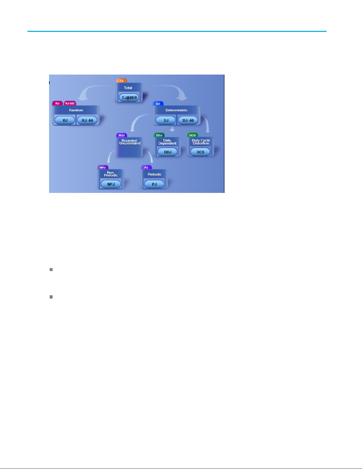
Perform advanced jitter and noise analysis (RJ, DDJ, PJ, DCD, BUJ, TJ@BER, and RN, DDN(high)
and DDN(low), BUN, TN@BER, vertical and horizontal eye opening at BER)
Perform mask testing on PDF eyes and BER contours
with advanced PAM4 signaling analysis, and 80SJNB with TDECQ (Transmitter and
Acquire complete pattern waveform at 100, 40, 20, or 10 Samples/UI
Perform random and deterministic jitter analysis including BER estimation
Isolate and measure crosstalk in form of bounded uncorrelated jitter (BUJ)
Display results graphically including histograms, spectra, and bathtub curves
Display 2-D eye diagrams (correlated eye, probability density function (PDF) eye, and bit error
ratio (BER) eye)
Save complete acquisition results to a data file
Analyze jitter, noise, and BER in the presence of spread spectrum clocking (SSC)
80SJNB Advanced includes everything in Essentials and adds:
Signal path emulation, allowing you to emulate the environment your signal encounters from the
transmitter to the receiver. Feature include:
Supports CTLE, FFE, and DFE equalization
Allows user-defined arbitrary filters (use for de-embedding, CTLE Transmitter equalization, and
other applications)
Supports channel emulation (TDR/TDT and S-parameter based channel descriptions)
Other features commonly known as SDLA (Serial Data Link Analysis)
80SJNB PAM4 includes everything in Advanced and adds:
Comprehensive jitter, noise and BER analysis for each eye
Global PAM4 signal characterization measurements
80SJNB Printable Application Help 1
Page 10

Welcome Welcome to the 80SJNB jitter, noise, BER, serial data link, PAM4, and TDECQ analysis software
Full signal path emulation support
Rise/Fall measurements
80SJNB TDECQ (Transmitter and Dispersion Eye Closure for PAM4) includes everything in PAM4
and adds:
Standard IEEE TDECQ measurements
Plots with annotations for the results
80SJNB prov
modules the DSA8300 supports. Accuracy is enhanced by allowing you to:
Chose to ap
Create BWE filters from S-parameters that characterize the target acquisition modules
Load BWE filters if previously generated
What do you want to do?
Read the product description
Go to Operating Basics
ides bandwidth enhancement (BWE) capabilities for the high bandwidth, low noise, optical
ply the BWE filters
(see page 7).
(see page 13).
2 80SJNB Printable Application Help
Page 11

Preface Related documentation
Related documentation
The following links contain other information on how to operate the oscilloscope and applications:
GPIB Information (see page 3)
Types of Help Information (see page 4)
GPIB information
For information on how to operate the oscilloscope and use the application-specific GPIB commands,
refer to the following items:
The programmers guide for your oscilloscope can provide details on how to use GPIB commands
to control the oscilloscope.
The 80SJNB remote control functions (see page 103)
Conven
Help t
tions
opics use the following conventions:
The terms “80SJNB application” or “application” refer to the 80SJNB Jitter, Noise and BER Analysis
are.
softw
The term “oscilloscope” or “TekScope” refers to the product on which this application runs.
The term “select” is a generic term that applies to the two methods of choosing an option: with
amouseorwiththeTouchScreen.
The term “DUT” is an abbreviation for Device Under Test.
Whenstepsrequireasequenceofselectionsusingthe application interface, the “>” delimiter marks
each transition between a menu and an option. For example, one of the steps to recall a setup file
would appear as File > Recall Settings.
80SJNB Printable Application Help 3
Page 12

Preface Types of application help information
Types of application help information
The application help contains the following topics:
Getting Started topics briefly describes the application and its requirements.
Operating Basics topics cover basic operating principles of the application. The sequence of topics
reflects the steps you perform to operate the application.
Parameters topics cover the Analysis and Configuration default settings.
Application Examples topics show how to use jitter measurements to identify a problem with a
waveform. This should give you ideas on how to solve your own measurement problems.
GPIB Command Syntax topics contain a list of arguments and values that you can use with the remote
commands and their associated parameters.
See also:
Using Help (see page 4)
Application help use
Application help has many advantages over a printed manual because of advanced search capabilities.
The main (opening) Help screen s hows a series of book icons and three tabs along the top menu, each of
which offers a unique mode of assistance:
Contents tab - organizes the Help into book-like sections. Select a book icon to open a section;
select any of the topics listed under the book.
Index tab - enables you to scroll a list of alphabetical keywords. Select the topic of interest to display
the corresponding help page.
Search tab - enables you to search the entire help contents for keywords. Select the topic of interest to
display the corresponding help page. Search results do not include text contained within illustrations
or screen shots.
OTE. Blue-underlined text indicates a hyperlink to another topic. For example, select the blue text to
N
jump to the topic on Feedback to Tektronix.
TIP. When you use a mouse, the normal cursor changes to a link cursor when over an active hyperlink.
(see page 5)
4 80SJNB Printable Application Help
Page 13

Preface Feedback
Feedback
Tektronix values your feedback on our products. To help us serve you better, please send us s uggestions,
ideas, or other comments you may have about your application or oscilloscope. Send your feedback to
techsupport
Please be as specific as possible and include the following information:
General information
@tektronix.
Oscillosc
Module and probe configuration. Include model numbers and the channel/slot location.
Serial data standard.
Signaling rate.
Pattern type and length.
Your name, company, mailing address, phone number, FAX number.
NOTE. Please indicate if you would like Tektronix to contact you regarding your suggestion or comments.
ope model number, firmware version number, and hardware/software options, if any.
Application-specific information
80SJNB Software version number.
Description of the problem such that technical support can duplicate the problem.
If possible, save the oscilloscope waveform fileasa.wfmfile.
ossible, save the 80SJNB data to a .mat file (File > Save Data).
If p
If possible, save the 80SJNB and oscilloscope settings to a .stp file (File > Save Settings).
Once you have gathered this information, contact technical support by phone or through email. If using
email, be sure to enter “80SJNB Problem” in the subject line, and attach the .stp and .wfm files.
80SJNB Printable Application Help 5
Page 14

Preface Feedback
6 80SJNB Printable Application Help
Page 15

Getting started Product description
Product description
The 80SJNB software application enhances the capabilities of the DSA8300 Digital Serial Analyzer by
providing Jitter, Noise, and BER analysis (Essentials) and features for de-embedding the fixture, channel
emulation, a
of PAM4 signals to 80SJNB Advanced including the TDECQ measurements.
nd FFE/DFE equalizer support (Advanced). The PAM4 option adds comprehensive analysis
You ca n u s e t
Jitter and noise analysis from DC to 400 Gb/s and beyond
Jitter and noise separation (see the Importance of Jitter and Noise Separation (see page 9))
Perform random and deterministic jitter and noise analysis, and TJ@BER, TN@BER and BER
estimation
Isolate jitter and noise due to crosstalk, and make random and deterministic estimations in the
presence of crosstalk
Show results as numeric and graphical displays
Display 2-D eye diagrams (Correlated Eye, Probability Density Function (PDF) Eye, and Bit Error
Rate (BER) Eye) for both NRZ and PAM4 signals
Perform mask testing on PDF eyes and BER contours
Support for CTLE, FFE and DFE equalization
Perf
Allow user-defined linear arbitrary filters
Support for Channel Emulation (from TDR/TDT and S-parameter based channel descriptions)
Analyze jitter, noise, and BER in the presence of Spread Spectrum Clocking (SSC)
his application to do the following tasks:
orm TDECQ (Transmitter and Dispersion Eye Closure for PAM4)
Save results to a PDF file
Save and recall instrument setups
See also:
Review Requirements and Restrictions (see page 7)
Requirements and restrictions
Operating system. Microsoft Windows 7 Ultimate (32 bit) operating system operating on the DSA8300
Digital Serial Analyzer oscilloscope.
80SJNB Printable Application Help 7
Page 16

Getting started Accessories
ADVTRIG option. 80SJNB requires the Advanced Trigger option (ADVTRIG). Contact Tektronix about
purchasing this option.
82A04/82A04B Phase Reference module. For acquisition in the presence of Spread Spectrum Clocking
(SSC), this application requires that the sampling oscilloscope be equipped with a Tektronix 82A04 or
82A04B Phase Reference module. The 82A04/4B also lowers the jitter floor to 100 fs. Contact Tektronix
about purchasing the module for your sampling oscilloscope.
Keyboard an
mouse is not required but simplifies screen selections.
Accessor
There ar
Tektronix website for information on optional accessories relevant to your application.
Asecon
screen and the 80SJNB application screen.
Refer t
application.
Conn
ecting to a device under test (DUT)
You c
d mouse. You must use a keyboard to enter names for some save and export operations. A
ies
e no standard accessories for this product. Refer to the product data sheet available on the
d monitor connected to the TekScope is recommended for simultaneous viewing of the oscilloscope
o Requirements and Restrictions
an use any compatible probe or cable interface to connect your DUT and the instrument.
(see page 7) for additional items required to use the 80SJNB
WAR NING. To avoid electric shock, remove power from the DUT before attaching probes. Do not touch
exposed conductors except with the properly rated probe tips. Refer to the probe manual for proper use.
Refer to the General Safety Summary in your oscilloscope manual.
See also:
Deskewing Probes and Channels (see page 9)
An Application Example (see page 88)
8 80SJNB Printable Application Help
Page 17

Getting started Deskewing probes and channels
Deskewing probes and channels
To be sure of accurate results for two-channel measurements, it is important to first deskew the probes
or cables and oscilloscope channels before you take measurements.
NOTE. Deskew
the DSA8300 Quick Start User Manual and the DSA8300 Help system for information and procedures for
deskewing probes and channels.
ing is performed from the TekScope application, not from the 80SJNB application. Refer to
The importance of jitter and noise separation
Jitter is an important characteristic to analyze for serial data links, but the analysis should not stop at just
jitter. To properly evaluate a data link, it is necessary to analyze both jitter and noise.
Two components need to be added to the traditional jitter analysis:
The nois
Jitter measurements based on the threshold crossing of a finite-speed transition should include vertical
noise i
Noise measurements and jitter a nd noise separation and reconciliation is performed on all 4 levels of
aPAM4
Depending on the magnitude of the vertical noise and the transient response of the transmitter and
smission channel, the magnitude of this influence can vary widely. Ultimately the jitter and noise
tran
analysis allows for accurate BER projections for the targeted communication link.
e/vertical eye closure should be considered similar to that of jitter/horizontal eye closure.
nfluence.
signal.
o w ww.tek.com/jitter for additional jitter and timing analysis information.
Go t
80SJNB Printable Application Help 9
Page 18
Getting started Jitter and noise separation methods
Jitter and noise separation methods
Bit error rates (BER) of a serial data stream are impacted by both jitter and noise. An accurate
decomposition of jitter and noise in the sources of impairments is critical to correctly estimate the signal
path behavior at larger BER. The jitter and noise maps are critical to help debugging the devices under test.
Since jitter and noise analysis follows a similar path, this discussion covers just the jitter decomposition.
The basic separation of jitter in data-dependent and uncorrelated elements is accomplished by two targeted
acquisition steps:
Correlated Acquisition Step: the application filters a high resolution acquisition of the full pattern
to eliminate the uncorrelated elements. The analysis of the filtered pattern yields the data dependent
characteristics, such as Data Dependent Jitter (DDJ) and Duty Cycle Distortion (DCD).
Uncorrelated Acquisition Step: the uncorrelated elements of jitter are isolated by acquiring on well
defined single spots in the pattern, thus eliminating the dependency on the pattern itself. The data
uired in the uncorrelated acquisition step is then further analyzed to isolate random unbounded
acq
components from the bounded deterministic components. This extended analysis is critical to help
predict long term behavior of the DUT.
Historically only spectral separation was used for separation (available still as the Spectral (Legacy)
analysis method). This method improperly qualifies certain complex bounded uncorrelated components as
unbounded, which inflates the random jitter (RJ) measurement result.
Spectral separation with isolation of bounded uncorrelated jitter (Spectral + BUJ) works by also
analyzing the cumulative distribution function (CDF) of the uncorrelated non periodic jitter data. In
the spectral separation of Periodic Jitter from the Random Jitter, the distinct spectral lines are removed
from the frequency domain representation of the global uncorrelated jitter data to quantify the periodic
jitter components, PJ. In the legacy method, the spectral method evaluated the remaining spectral data
as Random Jitter (RJ).
10 80SJNB Printable Application Help
Page 19

Getting started Jitter and noise separation methods
The presence of complex bounded uncorrelated impairments (for example, originating from crosstalk)
requires significant additional steps to isolate the bounded, uncorrelated jitter (BUJ) from the periodic jitter
(PJ), nonperi
The CDF analysis is performed in two s teps: before a nd after the spectral separation that identifies the
periodic spe
second analysis step yields the nonperiodic elements, and finally the random jitter components.
odic jitter (NPJ), and random jitter (RJ) components.
ctral components. The first analysis step yields the total bounded uncorrelated jitter, while the
A parallel a
the behavior of the link in terms of bit error ratio (BER).
nalysis track develops the noise map, and a combination of the two analysis tracks characterizes
80SJNB Printable Application Help 11
Page 20

Getting started Jitter and noise separation methods
12 80SJNB Printable Application Help
Page 21
Operating basics About operating basics
About operating basics
These topics cover the following tasks:
Navigating the user interface (see page 24)
User interface information (see page 22)
Using oscilloscope functions (see page 21)
Setting up the application (see page 28)
Viewing the measurement results as plots (see page 22)
Exporting Plot Files (see page 74)
Saving (see page 70) and recalling (see page 70) setup files
Saving (see page 71) and recalling (see page 71) data files
What do you want to do?
Start the 80SJNB Application (see page 13)
See also:
File Name Extensions (see page 17)
File Menus (see page 18)
Starting the 80SJNB application
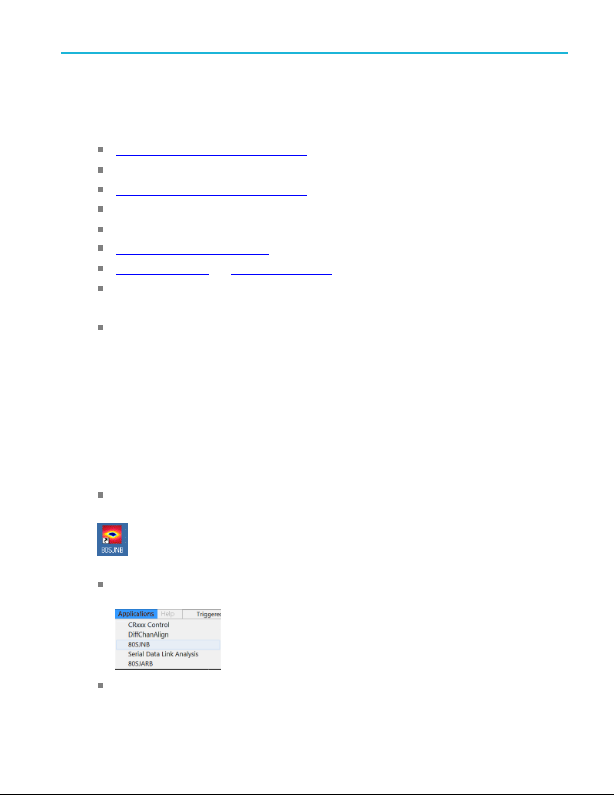
There are several ways to start the 80SJNB application.
If the TekScope application is minimized, double-click the 80SJNB application icon on the Windows
desktop to start the 80SJNB application.
If the TekScope application is running and open, select Applications > 80SJNB or 80SJNB
Advanced.
In Windows, select Start > All Programs > Tektronix Applications > 80SJNB > 80SJNB.exe.
80SJNB Printable Application Help 13
Page 22

Operating basics Returning to the oscilloscope application
TIP. With a second monitor connected to the TekScope, you can move the 80SJNB application d isplay to
the second monitor, allowing you to view both screens at the same time.
See also:
Returning to
Returning to the Oscilloscope Application (see page 14)
the 80SJNB Application
(see page 15)
Returning to the oscilloscope application
The 80SJNB application fills the entire screen and hides the TekScope application. To return to the
TekScope display, click the Back to Scope button
You can also minimize the 80SJNB application or exit the 80SJNB application entirely.
See also:
Minimizing and Maximizing the Application (see page 15)
Exiting the Application (see page 16)
in the toolbar.
14 80SJNB Printable Application Help
Page 23

Operating basics Returning to the 80SJNB application
Returning to the 80SJNB application
The TekScope application fills the entire screen. If the 80SJNB application is already running but the
TekScope application is displayed on top, bring the 80SJNB application to the front using one of the
following me
Click the App button on the TekScope toolbar.
Select Applications > Switch to 80SJNB.
thods.
TIP. If you have a keyboard attached, you can switch between running applications by pressing the Alt
+ Tab keys.
Minimizing and maximizing the application window
To minimize the application to the Windows task bar, select the command button in the application
bar.
menu
To maximize the application, select the minimized application from the Windows task bar. Alternately, if
have a keyboard attached, switc h between displayed applications by pressing Alt + Tab keys.
you
80SJNB Printable Application Help 15
Page 24

Operating basics Exiting the application
Exiting the application
To exit the application, select File > Exit or the command button in the application menu bar.
Software and file installation directory
The 80SJNB software is installed in the following directory:
C:\Progra
m Files\TekApplications\80SJNB
Save and recall directory
The directory structure for saving and recalling setup and data files and exporting data is:
C:\User
The default user name is:
Tek_Local_Admin
Standard masks are installed at:
C:\Users\Public\Documents\Tektronix\Masks
s\<user name>\Documents
See also:
File Name Extensions (see page 17)
16 80SJNB Printable Application Help
Page 25

Operating basics File name extensions
File name extensions
Extension Description
.bmp
.csv
.flt 80SJNB application filter file
.jpg
.mat
.msk
.png
.s1p
.s2p
.s4p
.stp
.tap
.txt
.wfm File that defines time domain waveforms or a frequency domain 1-port S-parameter (created
xxx
File that uses a bitmap format
File that uses a comma separated value format
File that uses a joint photographic experts group format
File that uses native MATLAB binary format to store data acquired by 80SJNB
Tektronix mask file (Mask file structure
File that uses a portable network graphics format
Files that define 1-port, 2-port, and 4-port frequency domain S-parameters
80SJNB application setup file
80SJNB application equalization tap file
File that uses an ASCII format
onnect) for channel emulation
by IC
80SJNB accepts both DSA8300 and IConnect .wfm files
(see page 99))
80SJNB Printable Application Help 17
Page 26

Operating basics File menu
File menu
The File menu lets you save and recall application setups, data files, and recently accessed files.
CAUTION. Do not edit a setup file or recall a file that was not generated by the application.
Menu item Description
Save Settings Saves the current application settings in a .stp fi le
Recall Settings Browse to select an application setup (.stp) file to recall; restores the application and oscilloscope
to the values saved
Save Data Saves the c urrent
Saving is disabled if there is no acquired data to save or an acquisition is in process
Recall Data
Export Results
Export Waveform Acquired exports the raw acquired pattern before processing of the data
Print Prints the displayed plots and all numeric results
Print to File
Exit Exits the application
xxx
Recall a saved data file for analysis
All plots and results are based on the recalled data
Recalling is dis
Exports jitter
Signal attributes and analysis configuration parameters are added to the report to qualify the
measurement results.
Correlated ex
Print the displayed plots and all numeric results to a .pdf file
See also:
in the setup file
acquired data in a .mat file for later analysis
abled if an acquisition is in process
and noise analysis results to a .csv format user specified file.
ports the acquired waveform after filtering out the uncorrelated components
About the 8
0SJNB Tool Bar
(see page 25)
Saving a Setup File (see page 70)
Recalling a Saved Setup File (see page 70)
SavingaDataFile(see page 71)
Recalling a Saved Data File (see page 71)
About Exporting Plot Files (see page 74)
18 80SJNB Printable Application Help
Page 27

Operating basics View menu
View menu
The View menu lets you configure the display of plots and/or numerical data. The menu contents depend
on the c urrent acquisition mode (NRZ, PAM4, or TDECQ).
NRZ acquisition mode View menu
Menu item Description
1-up Displays a single plot on the screen
2-up Displays two plots on the screen
4-up
Plots Only Hides all numeric data, expands the displayed plot(s) to fill the screen
Numeric Summary Displays the plots and a summary of the analysis results
Full Numeric Results
Global Results Displays a summary of Jitter and Noise measurements, Rise/Fall, and level measurements
JNB Results Displays the JNB Results tab, which contains the JNB results table
Mask Results Displays the Mask Results tab, which contains the Mask test results table
xxx
PAM4 acquisition mode View menu
Displays the maximum of four plots on the screen
Displays the plots and the full results table (JNB or Mask)
Menu i
tem
Descr
iption
1-up Displays a single plot on the screen
2-up Displays two plots on the screen
4-up
Displays the maximum of four plots on the screen
Plots Only Hides all numeric data, expands the displayed plot(s) to fill the screen
Numeric Summary Displays the plots and a summary of the analysis results
ll Numeric Results
Fu
Displays the plots and the full results table (JNB or Mask)
Global Results Displays the global PAM4 results tab containing global and summary information
NB Results: Eye0
J
NB Results: Eye1
J
JNB Results: Eye2
Displays the JNB Results tab for eye 0, which contains the eye 0 results table
Displays the JNB Results tab for eye 1, which contains the eye 1 results table
Displays the JNB Results tab for eye 2, which contains the eye 2 results table
Mask Results Displays the Mask Results tab, which contains the Mask test results table
Rise/Fall
Displays the Rise/Fall measurements and their statistical analysis
Measurements
xxx
80SJNB Printable Application Help 19
Page 28

Operating basics Setup menus
TDECQ acquisition mode View menu
Menu item Description
1-up
Global Results Displays 4 measurements: TDECQ, OMA Outer, ER, and AOP
Displays a single plot on the screen – TDECQ
NOTE. No other display configurations are relevant when View is set to TDECQ.
xxx
See also:
About the 80SJNB Tool Bar (see page 25)
Setup menus
The Setup menus provide access to the various configuration menus.
Menu item Description
tion
Acquisi
Signal Path Displays the Signal Path dialog screen to define the signal path characteristics to simulate the
Analysis
Test
Mask
Default Setup Returns the Acquisition, Signal Path, and Analysis settings to their default values
xxx
About the 80SJNB Tool Bar (see page 25)
Displays the Acquisition setup dialog screen to select and configure the source for measurements
and control key oscilloscope setups
conditions your signal may encounter
actual
ays the Analysis dialog screen to change settings that affect how measurements are made
Displ
and displayed
Displays the Mask Test Setup dialog screen to load a mask and define the mask test parameters
See About Application Parameters
u
men
(see page 95) to view the default settings for each configuration
20 80SJNB Printable Application Help
Page 29

Operating basics Oscilloscope settings
Oscilloscope settings
All relevant oscilloscope settings are accessible using the Acquisition dialog box of the 80SJNB
application.
To bring the TekScope application to the front of the display, click the Back to Scope button
or minimize the 80SJNB application. Alternately, you can use the Alt + Tab keys to switch between
applications if you have a keyboard attached.
See also:
About Con
Returning to the Application (see page 14)
Minimizing and Maximizing the Application (see page 15)
figuring the Application for Analysis
About the results
There are two ways to view analysis results: as numeric data and as graphical plots.
You can log the results data to .csv files for viewing in a spreadsheet, database, text editor or data analysis
program.
There a re several results tables: Global measurements, Jitter and Noise and BER analysis for each of the
eyes (3 for PAM4), Mask analysis re sults, and statistical analysis for the Rise and Fall measurements.
See also:
Working with Results (see page 83)
Clearing Results (see page 22)
(see page 28)
Exporting Plot Files (see page 74)
Exporting Results from the File Menu (see page 18)
80SJNB Printable Application Help 21
Page 30

Operating basics Clearing results
Clearing results
Click the Clear Data button to remove the existing plot displays and results. You may want to clear
the data before acquiring new data or between c ycles when the sequence mode is set to Free run.
NOTE. The numeric results and plot files are erased each time a new acquisition cycle is started.
About plotting
The application displays the results as plots for more comprehensive analysis. Before or after you take
measurements, you can select to display a single plot, two plots or four plots. You can select the type
of data you want to view in each plot window.
See also
Wo rking with Plots (see page 72)
Plot Type Definitions (see page 72)
About Working with Results (see page 83)
:
About the user interface
The application uses a Microsoft Windows-based user interface.
NOTE. The TekScope application is hidden when the 80SJNB application is running and not minimized.
22 80SJNB Printable Application Help
Page 31

Operating basics User interface items definitions
See also:
Starting the Application (see page 13)
Definitions of the application user interface items (see page 23)
Minimizing and Maximizing the Application (see page 15)
Exiting the Application (see page 16)
User interface items definitions
Item Description
Area
Box
Browse
Check box
Command button Initiates an immediate action, such as the Start command button in the Control panel
Keypad
Menu
Menu bar
Status bar Line located at the bottom of the application display that shows the acquisition status and the
Virtual keyboard
Visual frame that encloses a set of related options
Use to define an option; enter a value with the Keypad or a Multipurpose knob
Displays a window where you can look through a list of d irectories and files
Use to select or c lear an option
On-screen keypad that you can use to enter numeric values
All options in the application window (except the Control panel) that display when you select a
menu bar item
Located along the top of the application display and contains application menus
latest Warning or Error message
On-screen keyboard that you can use to enter alphanumeric strings, such as for file names
80SJNB Printable Application Help 23
Page 32

Operating basics About navigation
Item Description
Scroll bar Vertical or horizontal bar at the side or bottom of a display area that you use to move around in
that area
Tool bar
xxx
Located along
the top of the application display and contains application quick launch buttons
About navigation
The application provides you with several ways to display the results:
The drop-down menus available in the menu bar allows for screen configuration (one, two, or four
plots, summary or full numeric results table)
The buttons in the tool bar allow for screen configuration
The drop-down menus available in the plot display windows allow you to choose from the available
plots, and Copy, Examine, and Export plots
The status bar at the bottom of the screen contains progress information and displays error conditions
detected
Double clicking on a displayed graph opens the plot in a MATLAB window. MATLAB provides
additional display capabilities such as panning, zooming, data cursors, and 3D rotation. The Examine
button from the drop-down menu of the plot also opens the MATLAB window.
See also:
Windows User Interface (see page 22)
24 80SJNB Printable Application Help
Page 33

Operating basics About the 80SJNB tool bar
About the 80SJNB Toolbar (see page 25)
About Configuring the Application for Analysis (see page 28)
About the 80SJNB tool bar
The toolbar provides quick access to the most common functions you need to configure the settings, start
the acquisition, and control the numerical and plot displays. Most tasks are also available using the
drop-down lists from the File menu bar.
Acquisition button. Use the Acquisition button to select and configure the source for
measurements and control key oscilloscope setups. Any change in the Acquisition settings clears all
the data. The Acquisition button is disabled during the acquisition and processing cycle.
Signal Path button. Use the Signal Path button to define the signal path characteristics to
simulate the actual conditions your signal may encounter. Changes made in the signal path settings
does not clear the data, only the results. The Signal Path button is disabled during the acquisition
and processing cycle.
Analysis Setup button. Use the Analysis Setup button to change settings that affect how
measurements are made and displayed. Changes made in the analysis settings does not clear the
data, only the results are updated. The Analysis Setup button is disabled during the acquisition and
processing cycle.
Mask test button. Use the Mask Test button to select a mask and configure the mask test.
Free Run On/Off button. Use the Free Run button to select the sequence mode (free run on
or off).
When OFF, the button remains blue and the acquisition and processing cycle completes one pass
over the entire pattern. Off is the default mode.
When Free Run is ON, the button turns green
cycle repeats until stopped. The correlated components are averaged with previous data while the
uncorrelated components are accumulated for increased statistical content. At the
acquisition cycle, the plots and measurements are updated.
indicating that the acquisition and processing
completion of each
Free Run mode is recommended when:
There is a doubt that one acquisition cycle is enough. A change in the results indicate that additional
acquisition cycles was needed.
80SJNB Printable Application Help 25
Page 34

Operating basics About the 80SJNB tool bar
The correlated waveform shows irregular disturbances. It is possible that uncorrelated information
can leak into the single-pass correlated filtering. Acquiring a larger statistical sample improves
analysis in th
Several Standards specify the size of the data samples to be used for measurements. See the Stop on
Conditions s
e presence of crosstalk.
etup in Acquisition dialog.
To ha lt a Fr e
Sequence mode, so that the acquisition stops when the cycle is complete.
button is pressed, do not change any instrument settings. When the Run button is pressed, all current
measurement data and plot displays are cleared. During the acquisition and processing cycle, the
Signal Path, Analysis, Acquisition, and Run buttons are disabled.
During the acquisition and processing cycle, the Run button is replaced with the Pause button
Click Pause to interrupt the current acquisition and processing cycle. Click the button again to resume
the cycl
and proc essing cycle so you can view and save the measurement data between cycles.
Sequence mode, stopping the cycle produces no results and you must click the Start button to start a
new cycle.
is set to ON (cumulating previous data with new), you can clear the existing results and plots during
the processing cycle, thus starting a new acquisition and processing cycle.
Yo
e Run cleanly, deselect the
Run button. Use the Run button to start the acquisition and processing cycle. Once the run
e. This is useful when the acquisition is set to Free Run, allowing you to halt the acquisition
Stop button. Use the Stop button to end the acquisition and processing cycle. While in Single
Clear Data button. Use the Clear Data button to clear all results and plot displays. If Free Run
Plot Display buttons. Use the window pane buttons to display between 1, 2, or 4 plots.
u can change the number of plot displays at any time.
button. This converts the Free Run mode back to Single
.
meric Results Display button. The results button changes the display to a complete list of
Nu
statistics. If the application is displayed on a larger screen, the numeric results display shows all the
results at once.
Back to Scope button. Use this button to bring the TekScope display to the front of the screen.
See also:
About Configuring the Application for Analysis (see page 28)
About Analysis Settings (see page 54)
26 80SJNB Printable Application Help
Page 35

Operating basics About measurement results tabs
About measurement results tabs
The application shows several measurement results tabs depending on the coding of the signal (NRZ or
PAM4) being measured.
ThethreeNRZtabsarelabeledGlobal,JNBResultsandMask.Thesetabsshowthesamegraphsbut
display different numeric results. Global results display a summary of Jitter and Noise measurements,
Rise/Fall, and level measurements. Tab JNB Results displays all jitter, noise, and BER results. The Mask
plays all mask results such as hit ratio, margins, and BER limit.
tab dis
For PAM4 signals, six tabs are available. The Global tab displays both global PAM4 results and summary
s across all eyes. The JNB Results tab is replaced by three tabs, one per eye, labeled Eye0, Eye1 and
result
Eye2. Eye0 is the lowest eye. These tabs display all jitter, noise and BER results for their respective eyes.
The Rise/Fall tab displays the Rise/Fall measurements and their statistical analysis. When Fast TDECQ
mode is selected, measurements are limited to 4: TDECQ, OMA Outer, ER, and AOP.
The currently selected tab is labeled with a larger font. In addition, the three Eye tab labels are color
coded to match the figures having one graph per eye. In such figures, the yellow, green and red graphs
represent the data for eyes 0, 1 and 2, respectively.
80SJNB Printable Application Help 27
Page 36

Operating basics MATLAB user interface
MATLAB user interface
The 8 0SJNB application includes MATLAB®plots to provide further data analysis and visualization of
the plot displays.
MATLAB provides multiple capabilities to display and annotate the plot diagrams, including:
Pan and Zoom
2D and 3D visualization
Rotation
Data Curso
Color enhancements
MATLAB is a product distributed by MathWorks. You can view the MATLAB documentation and
tutorials on their Web site: http://www.mathworks.com
rs
About configuring the application for analysis
The tool bar provides an Acquisition (see page 29) button to configure the application to acquire data,
Signal Path
a
to change settings that affect how measurements are made and displayed, and a Mask test (see
page 99) button to set the mask test parameters.
NOTE. The Acquisition settings must be set before starting an acquisition cycle. You can modify the
Signal Path and Analysis settings without the need to reacquire data. You can also change the Mask
Test without the need to reacquire data.
28 80SJNB Printable Application Help
(see page 43) button to set signal path conditions, an Analysis (see page 54) button
Page 37

Operating basics About acquiring data
Use the Sequenc
run) or stop after one cycle is complete.
After setting up the application, you can select the Run button
cycle.
After the acquisition and processing cycle has completed, you can view the results as numerical
page 83) statistics or graphically (see page 22).
A typical scenario to setup the 80SJNB application and acquire data involves the following steps:
1. Set the Sou
2. Select Coding: NRZ or PAM4.
3. Set the number of Samples per UI.
4. Select a Stop on Condition.
5. Set the required Count.
6. From the tool bar, select Free Run mode.
7. Issue a
8. Wait until the 80SJNB application finishes running and then stops.
e button
rce, Data Rate, and Pattern Length.
Run command.
to have the acquisition and processing of data run continuously (free
to start the acquisition and processing
(see
See also:
tAcquiringData
Abou
(see page 29)
About acquiring data
Before making jitter and noise measurements, you need to select and configure the signal source.
e the Acquisition button
Us
In the Acquisition dialog box, select the signal source and signal coding (NRZ or PAM4), and define the
cquisition parameters. Some parameters (such as the Clock Recovery, Phase Reference Sources, and the
a
optical signal conditioning) are copied from the oscilloscope state.
Click the AutoSync to Selected Source button to have the 80SJNB application automatically obtain and
enter the following information from the signal applied to the channel defined as the Signal Source:
Data Pattern Rate
Data Pattern Length
Recommended Data:Clock Ratio (when Spread Spectrum Clocking (SSC) signaling is used)
to display the Acquisition dialog box.
80SJNB Printable Application Help 29
Page 38

Operating basics About acquiring data
NOTE. Acquisition in the presence of SSC requires certain cabling propagation delays to be preserved.
Please contact Tektronix for an up-to-date diagram of cabling lengths.
One of the key acquisition parameters is the number of samples per unit interval. The default is 100
samples per unit interval. For higher throughput and support of longer record lengths than PRBS13, you
can optional
The Fast TDECQ acquisition m ode is optimized to return TDECQ measurements in minimum time. The
Number of Sa
Random Quaternary), equivalent to PRBS16, the maximum number per UI is 10. For pattern lengths
shorter than PRBS13Q, this could be set to 20, 40, or 100.
The acquisition only mode (Acquire (ONLY) All Optical Channels) that when enabled, acquires all
available optical channels in the instrument at the same time. Once the acquisition is complete, save the
acquired data files for a n alysis at a later time. Go to File > Save Data to save the acquired data from
all channels.
NOTE. Tektronix recommends running this functionality in the oscilloscope (the equivalent menu exists in
Setup >
UI/PI allows manual entry of some of the parameters of the AutoSync, which dramatically improves the
success rate of AutoSync. For example, manually entering the Data Pattern Length, and then unchecking
the pattern length item from the AutoSync search, makes the data pattern length much more likely to
succeed. Refer to the DSA8300 TekScope application help for details about the Pattern Sync settings.
ly select 40 samples per unit interval.
mples per UI defaults to 10, and can be set to 5. For standard SSPRQ (Short Stress Pattern
Mode/Trigger > Pattern Sync/FrameScan Setup). The important difference is that the oscilloscope
See also:
Selecting the Source (see page 40)
30 80SJNB Printable Application Help
Page 39

Operating basics Selecting a Stop on Condition
Selecting the Data Pattern (see page 35)
Selecting a Stop on Condition (see page 31)
Selecting Scope Setup Recall On Exit (see page 32)
Scope Noise (see page 36)
BWE (see page 36)
Selecting the Signal Conditioning (see page 35)
Selecting the Pattern Clock (see page 39)
Selecting Clock Recovery (see page 33)
Selecting Phase Reference (see page 34)
Analysis Settings (see page 54)
Selecting a Stop on Condition
The Stop on Condition selections allow you to control the amount of data to be acquired and processed
before stopping.
NOTE. The Free Run mode has to be selected for the Stop on Conditions to be active. Use the Sequence
button
There are four options to control the stop condition:
Never. This is the default condition. The acquisition and processing of data runs continuously until
explicitly stopped by u ser by clicking on the Stop button.
Acquisition cycles. Acquisition Cycles instructs the 80SJNB application to continue acquiring and
processing data until the defined number of cycles have completed. Note that changing the number of
Acquisition Cycles coerces the numbers associated with the o ther two options. Each acquisition cycle
includes a number of uncorrelated samples, selected by design, and a number of samples correlated with
the d ata pattern, which depends on the pattern length and the number of samples per data bit – which is
also selected by design.
The following equation describes the relationship between these parameters:
Total Population Limit = Acquisition Cycles * (Uncorrelated_Samples_Per_Cycle + Samples_Per_Bit
* Pattern_Length)
to select the continuous acquisition and processing mode.
Uncorrelated samples. Uncorrelated Samples instructs the 80SJNB application to continue acquiring and
processing data until the data required for jitter and noise processing exceeds the specified number. The
default count is a number that represents 2 acquisition cycles.
80SJNB Printable Application Help 31
Page 40

Operating basics Selecting scope setup recall on exit
Total population limit. Total Population Limit instructs the 80SJNB application to continue acquiring and
processing data until the total number of samples exceeds the specified number. The default count is a
number that re
The actual number of acquired and processed samples is displayed in Sample Count (see below), and
corresponds
presents 2 acquisition cycles, and re fl ects the selected Pattern Length.
to the nearest integer number of acquisition and processing cycles.
Selecting scope setup recall on exit
Acquiring data for jitter and noise analysis requires the 80SJNB application to fully control the
oscilloscope state. When this control is checked, exiting the 80SJNB application (File > Exit) restores the
oscilloscope to the state which was stored when 80SJNB application was launched.
32 80SJNB Printable Application Help
Page 41

Operating basics Selecting clock recovery
Selecting clock recovery
The Advanced Trigger option (ADVTRIG) that generates the pattern synchronous triggers requires a
clock source synchronous with the signal. When using a clock derived from a clock-recovery module
installed in
source module, the configuration and its frequency.
All native clock recovery modules support two different configurations: one that connects the recovered
clock from the back of the module to the internal pattern synchronous trigger generator; and, for optimal
jitter p
Input.
the oscilloscope (such as optical sampling modules), use the Pattern Clock fields to select the
erformance, the module full rate clock output can be connected to the front panel Clock/Prescale
These s
The Rate setting is limited to the capabilities of the selected module. The numeric keypad is unavailable
for use
ettings are grayed out if no modules with clock recovery are detected at application startup.
unless the module can accept USER defined rates.
80SJNB Printable Application Help 33
Page 42

Operating basics Selecting phase reference
Selecting phase reference
You can use a Phase Reference module (such as the Tektronix 82A04B) to reduce the trigger jitter of the
signal source, thus increasing the jitter measurement accuracy. If analyzing a signal using Spread Spectrum
Clocking (SS
If using a Phase Reference module, set the channel source and the frequency of the applied clock.
These settings are grayed out if a Phase Reference module is not detected at application startup. If a Phase
Reference module is detected, you have the option to not use the module by selecting None as the Source.
C), a Phase Reference module is required.
TIP. Selec
Jitter) and the correlated waveforms. However, the throughput is lowered in this mode.
NOTE. W
frequency when the data was acquired. The Source field remains unchanged regardless if phase reference
was used when the recalled data file was created.
ting a Phase Reference module dramatically improves the accuracy of DDJ (Data Dependent
henusingarecalleddatafile, the Phase Reference Frequency field is updated to indicate the
34 80SJNB Printable Application Help
Page 43

Operating basics Selecting the data pattern
Selecting the data pattern
Defining the Data Pattern requires that you define both the data rate of the signal source and the pattern
length in bits. You can choose the data rate from a predefined set of lengths or enter a value with the
numeric keyp
NOTE. Selecting a data rate that does not match the communication standard that is set in the instrument’s
Horizontal Communication Standard setting dialog box causes the oscilloscope setting to change to User.
When selecting the pattern length, only the length is important. The precise bit sequence is unimportant
if it is repetitive.
To analyze a clock pattern, select a 2 bits pattern (or a multiple). The analysis is performed on both edges.
ad.
NOTE. Whenusingarecalleddatafile, the Data Pattern fields are updated to indicate the state of the
settings when the data was acquired.
Selecting the signal conditioning
Wavelength, Filter, Bandwidth
Use this control to select what type of fi ltering, if any, you want performed on the selected channel. The
available filters depend on the capabilities of the module.
If the Filter is set to None, you can use the Bandwidth box to select the bandwidth of the channel. The
available bandwidth selections depend on the capabilities of the module. Refer to the documentation for
the module about its filter or bandwidth settings.
80SJNB Printable Application Help 35
Page 44

Operating basics Selecting the signal conditioning
The list of hardware filters are specific to the selected module as data source. A comprehensive list of the
hardware filters, the standards they support, and the data rates, are listed in the DSA8300 Programmer
Manual. The ma
particular filter.
nual specifies the token names that are used by the programmatic interface to select a
The range and
type, probe type if attached, and an external attenuation factor. Use the DSA8300 programmatic interface
commands when an externa l attenuation factor is required. See the DSA8300 p roduct documentation
for details.
resolution of scale values for a selected channel is dependent on multiple factors: module
Scope Noise
Scope N oise is a relevant parameter for the TDECQ measurement. For optical modules, enter scope
noise in μW. For electrical modules, enter scope noise in μV. The default setting is dependent on the
acquisition module.
TDECQ measurements require you to specify the amount of scope noise contributed to the signal, DUT,
noise. Channel noise depends on type of the module and Signal Conditioning configuration: Wavelength,
Filter, Bandwidth.
Default noise values are loaded based on the selected module and its configuration.
You can measure and enter the scope noise manually, or use the Scope Noise Characterization utility,
installed on the instrument, to measure the scope noise. Access to the utility is from the DSA8300
Applications pull down menu.
The utility creates a scope noise file that can be imported by the 80SJNB application. Open the a pplication,
select all modules of interest and launch the Measure process. The results are stored in a file called
ScopeNoiseDB.ini located at C:\Users\Public\Tektronix\TekApplications.
When Scope Noise Import is selected, 80SJNB imports the scope noise measured for the user specified
Signal Conditioning configuration.
BWE
BWE (Bandwidth Enhancement) is a process of creating and applying a digital filter with the following
goals:
NOTE. Bandwidth Enhancement is currently for use with optical modules: 80C17, 80C18, 80C20, and
80C21.
36 80SJNB Printable Application Help
Page 45

Operating basics Selecting the signal conditioning
Improve the module reference receiver filters to more closely match an ideal response, specified by
Standards as 4th order Bessel-Thomson (BT).
Enable non-standard receiver rates or bandwidths.
Increase or decrease the bandwidth of the optical channel.
Specifically, for the 80C17 and 80C18 optical modules, BWE provides a bandwidth boost. For the
80C20 and 80C21 optical modules, BWE shapes the transfer function to approach as much as possible
to 4th order BT response.
The BWE filters are created from the S-parameters of the module.
Each module configuration, (wavelength, filter, and bandwidth) has an equivalent s1p S-parameter file.
Based on the Signal Conditioning configuration selected, the appropriate file needs to be selected when the
BWE filter is created.
The S-parameters are available (on a USB flash drive) for the following modules.
80C17 and 80C18: S-parameters available as an option at the time of purchase.
80C20 and 80C21: S-parameters provided at the time of purchase.
he Configure Filter button to either load an existing filterorcreateanewfilter.
Press t
80SJNB Printable Application Help 37
Page 46

Operating basics Selecting the signal conditioning
Load From File. Load From File allows you to apply a previously created filter. Use the Browse button to
navigate to the saved filter file.
Create Filter. C
Enter a filter name in the dialog screen.
Set the Data Rate of the signal.
Navigate to an S-parameter file that matches the optical module’s attributes.
Set the Target Bandwidth to the 3 dB bandwidth for the Bessel-Thompson filter. The default is 0.5 of
theBaudrateofthesignal.
Set the Bandwidth Limit that specifies the roll-off frequency of the BWE filter. The default is 0.9 of
theBaudrateofthesignal.
Youhavetheoptiontosavethecreatedfilter (Save Filter) for use at a later time or to apply it during
the next acquisition (Apply).
38 80SJNB Printable Application Help
reate Filter allows you to create a new filterbasedontheparametersyouset.
Page 47

Operating basics Selecting the pattern clock
NOTE. When saving the acquired data (using File > Save Data), the data patterns are saved without the
bandwidth enhancement but the bandwidth enhancement parameters are saved in the context. When
the saved data
Signal Path to apply the BWE.
is recalled, the bandwidth enhancement is reapplied. The Filter must be inserted in the
Selecting t
The Pattern
theAdvancedTriggerOption(ADVTRIG),isdrivenbythePatternClock.
The availa
Clock/Prescale Input, and this selection is available for all configurations. Connect the clock source to
the CLOCK INPUT/PRESCALE TRIGGER front-panel connector.
When the oscilloscope is equipped with one or more clock recovery capable modules, the CR units are
also available as sources for the Pattern Clock.
Each native clock recovery source appears on the Pattern Clock source list twice to allow for two different
configurations:
Selecting Cx Clock Recovery sets the instrument to pick up the recovered clock from the back
of the module using and internal signal path.
Selecting Cx CR to Clock/Prescale Input sets the instrument clock recovery signal source to the
CLOCK INPUT/PRESCALE TRIGGER connector on the front panel. Connect the output of the clock
recovery module to the front panel CLOCK INPUT/PRESCALE TRIGGER input.
Depending on the data rate, choosing one configuration over the other could result in different intrinsic
jitter performance. See Selecting Clock Recovery
particular cabling setup is necessary; only external Clock Recovery (such as with a Tektronix CR286A)
can be used. If the Tektronix 82A04/82A04B Phase ReferencemoduleisusedintheabsenceofSSC,
e 82A04/82A04B setup determines the jitter performance. The intrinsic jitter of the pattern trigger
th
circuit becomes invisible.
he pattern clock
Sync built-in capability provides user pattern synchronous triggers. The feature, enabled by
ble Pattern Clock sources depend on t he instrume nt configuration. The default selection is
(see page 33). In general, if there is SSC then a
When the clock source is a dedicated Clock Recovery Unit, like the Tektronix CR125A, CR175A,
or CR286A, the instruments are controlled b y a USB-link to the oscilloscope. The syntax of the
programmatic interface is specified in the DSA8300 Programmer Manual. The header of the commands
are TRIGger:CLCRec:CRC.
80SJNB Printable Application Help 39
Page 48

Operating basics Selecting the source
Selecting the source
The application takes measurements on waveforms specified as sources (also called signal sources). The
source can be a channel (CH1 through CH8) or a definedmathwaveform.Youcanuseanydefined math
waveform, wh
application.
ether it is definedinthe80SJNBconfiguration as a differential setup or in the TekScope
Specify whe
NOTE. Selecting PAM4 disables SSC.
If your si
application can make accurate measurements that account for clock rate modulation
NOTE. If a saved data file is recalled, the signal s ource selection remains unchanged but all result
panels will indicate the recalled data file as the source. The “SSC is present” field is updated to match
the se
ther the source waveform is NRZ or PAM4.
gnal source uses Spread Spectrum Clocking (SSC), select the SSC check box so that the
tting from the recalled data file.
See also:
About Spread Spectrum Clocking (SSC) (see page 41)
king the Diff button displays the dialog box to create a differential Math waveform by defining a
Clic
positive and negative waveform source (the negative waveform source is subtracted from the positive
waveform source). This generates a single mathematical waveform that the 80SJNB application can use
as the waveform measurement source.
40 80SJNB Printable Application Help
Page 49

Operating basics About spread spectrum clocking (SSC)
About spread spectrum clocking (SSC)
Spread Spectrum Clocking (SSC) is the technique of modulating the clock frequency to minimize EMI
effects. SSC affects the analysis process and the results of jitter, noise and BER measurements. If SSC
is not corrected for its effects, the results show as a large amount of periodic jitter components that are
reflected in the total jitter and noise, and ultimately in the BER estimates.
When SSC is present, 80SJNB measures the attributes of SSC and corrects the results.
SSC configuration requirements
NOTE. SSC is available only for NRZ coding measurements.
If using clock recovery, the clock recovery unit must be able to handle SSC. Use one of the Tektronix
BERTScope clock recovery instruments if SSC is present in the signal.
The TekScope must have an 82A04 or 82A04B Phase Reference Module installed. The module minimizes
the effect of the SSC on the data by sampling synchronously the data and clock. Also, by acquiring
the clock in the 82A04/4B module, 80SJNB characterizes the SSC present in the clock and uses that
information to correct the jitter, noise, and BER measurements performed on the data.
TIP. The “SSC is present” check box is disabled if the Phase Reference module is not installed in the
instrument.
Use the following settings to optimize the SSC phase correction for the signal you are measuring:
80SJNB Printable Application Help 41
Page 50

Operating basics About spread spectrum clocking (SSC)
Clock recovery
Data rate range
frequency
2
500 Mbps – 1 Gbps Data Rate * 4 Standard
1 Gbps – 2 Gbps Data Rate * 2 Standard
2 Gbps – 4 Gbps
4 Gbps – 8 Gbps
8 Gbps – 12.5 Gbps
xxx
1
The Clock R
2
Clock recovery is typically provided from a CR125A, CR175A, or CR286A BERTScope Clock Recovery Instrument.
When you i
ecovery unit clock output is either Standard or Subrate Clock.
nstruct 80SJNB that the data has SSC (by checking the “SSC is present” check box), the
Data Rate
Data Rate
Data Rate
Clock recovery
output rate
1,2
Standard
Subrate (1/2)
Subrate (1/4)
Data:Clock rat
(JNB)
1:4
1:2
1:1 Data Rate
2:1
4:1
io
Phase referenc
frequency (JNB)
Data Rate * 4
Data Rate * 2
Data Rate/2
Data Rate/4
e
following constraints are enforced based on the current Data Rate:
Phase Re
ference source is selected.
Phase Reference frequency is set to the recommended value in the table Configuration Settings for SSC.
A recommended Data:Clock Ratio is displayed to suggest the recommended subrate clock.
NOTE. Changes to the Data Rate are reflected in the Phase Reference Frequency and Data:Clock Ratio.
You mu
st make the appropriate changes to the Clock Recovery unit parameters.
The Full Numeric Results page shows the status (on or off) of the SSC setting. The results of the SSC
ysis are presented in two forms, numeric results and a plot. When viewing the full numeric results
anal
table, the SSC Modulation section has two fields: Magnitude and Frequency. Magnitude represents the
depth of the SSC clock modulation in parts-per-million (ppm) and Frequency reflects the SSC modulation
frequency.
To view the plot of the SSC modulation profile, select the Plot>SSC>SSC Profile.
TIP. The configuration settings are also available through the GPIB programming interface of the
oscilloscope. Refer to the information provided with the oscilloscope.
42 80SJNB Printable Application Help
Page 51

Operating basics About Serial Data Link Analysis (SDLA) Signal Path Settings
About Serial Data Link Analysis (SDLA) Signal Path Settings
The Signal Path Settings are available for use with the 80SJNB Advanced and PAM4 versions. If you
are using the 80SJNB Essentials version, you're allowed to use the dialog boxes but are not allowed
to place any o
The Signal Path settings allow you to emulate the environment your signal encounters, all the way from
the transmi
from the transmitter (Tx) to the Receiver (Rx). Along this line, you have the ability to emulate an arbitrary
filter and/or a channel. You can then define an equalizer to compensate for the effects the filter and channel
introduce. Also, fixture de-embed is supported.
f the functions into the signal path.
tter to the receiver. With the Signal Path dialog box, your signal path is represented by a line
Selecting a signal path arrow (Filter, Channel, or Equalizer) inserts or removes the function from the signal
path. When inserting a function into the signal path, its dialog box automatically displays.
Selecting a signal path button (Filter, Channel, or Equalizer) displays the dialog box for that function
without inserting or removing the function from the signal path.
imulating the signal environment, you can effectively emulate probing the signal at the receiver rather
By s
than the output of the transmitter. With the use of the Equalizer, you can then design compensations to
improve the signal quality at the receiver.
Full signal path functionality supports PAM4 signals.
80SJNB Printable Application Help 43
Page 52

Operating basics Setting Filter Conditions
TIP. You ca
To learn more about each of the signal path settings, select the following:
Filter
Channel (see page 45)
Equalizer (see page 48)
n move a function in and out of the signal path without affecting any settings.
(see page 44)
Setting Filter Conditions
The Signal Path Filter allows you to specify an arbitrary linear FIR filter to be applied to the acquired data
pattern. For instance, the transmitter may artificially enhance the signal at certain frequencies to overcome
known problems in the channel. You can use a filter to emulate this action or compensate for transmitter
signal pre-emphasis. Use the filter to insert a continuous-time linear equalizer (CTLE) in the signal path,
which standards typically specify for PAM4 signaling.
You c a n define or load a CTLE from the Equalizer. Inserting a de-embed filter is the most common
use o f the Filter. Use the SDLA (Serial Data Link Analysis) tool to generate the de-embed filters. See
tails below.
de
To use the filter, move the Filter function into the signal path and use the Filter file box or browse button to
pecify the filter file. The default location for the filter files is in the Windows/Documents folder. A few
s
filter files are provided as examples, but you are responsible for providing the filter files.
o use the Filter block for de-embedding, you will need an additional software tool to create a
T
de-embedding filter from the S-parameters of the fixture. Please visit the www.tektronix.com/sdla
site, or contact Tektronix Support for details.
44 80SJNB Printable Application Help
Web
Page 53

Operating basics Setting Channel Conditions
See Uncorrelated Scaling (see page 54) for information about this setting.
The following is an example of the filter file format:
@ 5.7e-005, 2.4e-005, 5.4e-005, 2.1e-005, 5.1e-00 5
The '@' means that it is valid for all frequencies.
Up to 20,000 coefficients may be specified.
Setting Channel Conditions
The Signal Path Channel allows you to emulate the channel (interconnect or lane) carrying the signal.
There are two ways to define the channel, w ith Time Domain
Domain (see page 45) S-parameters.
See Uncorrelated Scaling
Frequency Domain
With Frequency Domain selected, the channel is defined with an S-parameters file. Use the file selection
box or Browse button to select the file. The default location for the files are in the Windows/Documents
folder. You are responsible for providing the S-parameters file.
(see page 47) waveforms and Frequency
(see page 54) for information about this setting.
The S-parameters file can contain data for 1-port, 2-port, or 4-port devices. Once a file is selected,
the application reads its contents and generates the appropriate dialog for you to select the particular
S-parameter in the file to use.
80SJNB Printable Application Help 45
Page 54

Operating basics Frequency Domain
1-Port. Files with 1 port of data contain only 1 S-parameter so they do not require any further input. These
files may be IConnect 1-port files or Touchstone 1-port files.
2-Port. Files with data for 2 ports contain 4 S-parameters as a 2x2 matrix. These are Touchstone 2-port
files. When the application recognizes such an S-parameter file, a dialog is created for you to select the
S-parameter representing channel transmission. The typical selection is S
, and is the default selection,
21
but this may need to be changed if the file contains a 2x2 subset of the 4x4 matrix of S parameters defining
a 4-port system.
4-Port. Files with data for 4 ports may contain single-ended or mixed-mode data. These are Touchstone
4-port files.
If the data is single ended, you must map the port numbers as used in the file to physical locations in your
link. A default mapping is assumed. The application will use this mapping to compute the S
parameter
dd21
(for transmission of a differential signal) from the appropriate four S-parameters measured using single
ended data.
If the data is mixed mode, you must select the data layout in the file. The most common layout is DC12
and is the default selection. The application always uses the S
parameter for computing the transmitted
dd21
waveform no matter which mapping is selected.
46 80SJNB Printable Application Help
Page 55

Operating basics Time Domain
NOTE. 80SJNB Advanced uses the 'insertion loss' information only.
Time Doma
With Time
behavior. Use the fi le boxes or browse buttons to select the files you want to use. The default location
for the files is in the Windows/Documents folder. You are responsible for providing the time domain
waveform files.
NOTE. We recommend that the waveform file be a measurement of the channel from a Tektronix TDR/TDT
system. Required raw oscilloscope waveforms are:
a. A reference throughput (no DUT is inserted, just a throughput connection between the TDR step
source and the acquisition channel on the TDT end).
b. A DUT throughput measurement (the TDR step sou rce and the TDT acquisition channel are connected
through the DUT).
in
Domain selected, the Reference waveform and Transmitted waveform generate the channel
80SJNB Printable Application Help 47
Page 56

Operating basics About the Equalizer
About the Equalizer
The equalizer compensates for transmission channel impairments in the form of frequency-dependent
amplitude and phase distortions resulting in intersymbol interference (ISI) in the communication data
stream.
80SJNB provides tools to support three types of equalizers: CTLE (Continuous Time Linear Equalizer),
FFE (Feed Fo
equalizer (FFE) is defined by a user specified number of taps, taps per symbol (or unit interval), and the
weight of each tap. The equalizer becomes a decision-feedback equalizer (DFE) when the number of DFE
taps is set to a number larger than 0.
NOTE. Tap values and weights are used interchangeably.
rward Equalizer), and DFE (Decision Feedback Equalizer). The linear feed-forward
To learn about setting up the Equalizer, see:
Continuous Time Linear Equalizer CTLE
Equalizer Taps (see page 50)
48 80SJNB Printable Application Help
(see page 49)
Page 57

Operating basics Continuous Time Linear Equalizer (CTLE)
Uncorrelated Scaling (see page 54)
Continuous Time Linear Equalizer (CTLE)
The equalizer includes an optional filter that is intended to be a Continuous Time Linear Equalizer.
However, when loading the equalizer from a filter file (extension .flt) any filtermaybeused.Iftheradio
button Define CTLE is selected the user can define a 1- or 2-stage CTLE.
The schematic in the CTLE Definition dialog portrays each stage (assuming 2 poles per stage) of the CTLE
filter. The plotted function schematically shows the frequency response of the filter.
You can select a standard with a specified peaking in dB, which automatically fills in the remaining
parameters of the dialog, or manually define the remaining parameters of the dialog.
ADCis the gain at DC.
fZis the frequency of the zero of the filter.
80SJNB Printable Application Help 49
Page 58

Operating basics Equalizer Taps
fP1is the frequency of the first pole.
For a 2-pole stage, fP2is the frequency of the second pole. For a 1-pole stage, fP2is not defined.
When 2 stages are defined, the filters defined by the separate stages are convolved to produce the filter.
NOTE. Clicking Apply or OK causes the filter to be included in the updated definition of the Equalizer, but
when you exit this dialog and return to the Signal Path – Equalizer dialog, you must click Apply or OK
there, too, in order for the updated definition to now define the Equalizer. In addition, the Equalizer must
be made acti
ve for its definition to be used at all.
Equalizer Taps
The behavior of the equalizer is controlled by the number of taps and the tap values. Using the equalizer
requires
incorporate an equalizer filter delay by specifying a reference tap to compensate for precursor channel
effects.
that you specify the number of FFE and DFE taps, and the FFE spacing of the taps. You can also
You can manually set the FFE and DFE tap values, or you can use the Autoset Taps button to let the
application calculate the tap values.
FFE Taps description
Go to
Go to DFE Taps description (see page 51)
(see page 50)
FFE Taps
FFE Taps are weights applied to a set of samples taken from the data stream to compensate for
The
channel impairments manifested in the form of ISI. The number of FFE Taps represent the length of
history in data samples that contribute to the computation of a current bit. Data stream samples could
be distanced at unit intervals, in which case the number of FFE taps represents the number of preceding
bits that contribute to the correction of the current bit. Alternatively, the data stream could be sampled
at a higher rate per bit, yielding a fractionally-spaced FFE tap set.
50 80SJNB Printable Application Help
Page 59

Operating basics Equalizer Taps
The number of FFE taps defaults to 1, with the capability to specify up to 100 taps. The default FFE tap
spacing is at unit intervals. You can configure up to 10 taps per symbol.
The FFE Tap values could be specified by you using the FFE Taps dialog, or computed by the application
with the Autoset Taps button.
Go to Autoset Taps description
Go to Saving and Loading Taps (see page 53)
Pressing the FFE Taps button displays a dialog showing the current FFE tap values. You can specify each
FFE tap coefficient individually. Pressing the Defaults button sets the first FFE tap to 1 and the rest to 0.
(see page 53)
You can use the Save Taps button to save a set of coefficients to a file. Use the Load Taps button to load
saved Tap files.
DFE Taps
DFE taps are weights applied to the previous digital decisions made by the slicer (comparator + latch). The
number of DFE Taps specifies the number of bits contributing to the current input to the slicer. The default
number of DFE Taps is 0, in which case the equalizer is a linear FFE one. The maximum number of DFE
Taps is 40. Weights are scalars specified by you or computed by the Autoset Taps function.
80SJNB Printable Application Help 51
Page 60

Operating basics Equalizer Taps
See Autoset Taps (see page 53) for a description about u sing the autoset taps function.
Pressing the DFE Taps button displays a dialog showing the current DFE tap values. You can specify each
DFE tap coefficient individually. Pressing the Defaults button sets all DFE tap values to 0.
You can use the Save Taps button to save a set of coefficients to a file. U se the Load Taps button to
recall saved Tap files.
TIP. When
using the Equalizer, you are required to always have at least 1 FFE tap. DFE taps are optional.
Filter Settings
FFE Reference Tap. The FFE Reference Tap is a filter delay in unit intervals that should be set to
compensate for the delay between the transmitter output and the equalizer input. The value of the
nce Tap is constrained by the number of FFE Taps and the number of taps per symbol.
Refere
DFE Rise Time Selector. The Rise Time Selector specifies the Gaussian filter used to emulate the DFE
feedback path band-limited behavior. The rise time defaults to Track Data Rate, in which the configuration
is set to 1/5 of the unit interval equivalent with the data rate. Track tap interval designs a Gaussian filter
with a rise equal to 1/5 of the spacing between taps. Selecting User allows you to specify the rise time
1psto4ns.
from
Uncorrelated Scaling. See Uncorrelated Scaling
(see page 54) for a description.
52 80SJNB Printable Application Help
Page 61

Operating basics Autoset Taps
Autoset Taps
The tap autoset function computes a set of tap values that optimize the eye opening for the data pattern
applied to the input of the equalizer. If the DFE tap number is 0, the algorithm yields an optimal set of FFE
taps, while i
jointly optimizes the forward and feedback loop tap coefficients. The optimization algorithm is the
least-mean-square error (LMS) and the optimization targets the signal to noise ratio at the sampling phase.
The Autoset Taps will account for the FFE Taps/Symbol and Reference Tap specifications.
f the equalizer is specified as a DFE by a positive DFE tap number, the Autoset Taps algorithm
The tap aut
algorithm. The optimization algorithm is the least-mean-square error (LMS) and the optimization targets
the signal to noise ratio at the sampling phase. If TDECQ computation is enabled, the Autoset Taps
performs an MMSE (minimum mean square error) optimization according to the IEEE standard.
NOTE. You can autoset tap values even if the Equalizer is not inserted in the signal path.
oset algorithms computes a set of FFE and DFE taps using a least-mean-square optimization
Saving and loading taps
Use these controls to save or load a set of taps from a file. The browse director y defaults to Windows/My
Documents and the file extension is .tap.
The file format is the following:
<Tektronix>
<TapFile>
<FFE>
<TapsPerSymbol>value<\TapsPerSymbol>
ferenceTap>value<\ReferenceTap>
<Re
<Tap1>value<\Tap1>
<Tap2>value<\Tap2>
...
<Tapn>value<\Tapn>
</FFE>
DFE>
<
<Tap1>value<\Tap1>
<Tap2>value<\Tap2>
...
<Tapn>value<\Tapn>
</DFE>
</TapFile>
</Tektronix>
80SJNB Printable Application Help 53
Page 62

Operating basics Uncorrelated scaling
Uncorrelated scaling
The signal path settings (Filter, Channel, Equalizer) each have an uncorrelated scaling setting. The
Uncorrelated Scaling value multiplies the uncorrelated random noise RMS and uncorrelated periodic noise
values. Unco
The 80SJNB Signal Path does not process uncorrelated noise in any other way.
rrelated noise scaling affects the uncorrelated jitter as projected through the average slew rate.
If you inser
and set the Uncorrelated Scaling factor to its minimal value (0.01), the configuration will isolate the
effects of noise on jitter measurements. This configuration produces results that correlate with “jitter
only”typeanalysistools.
NOTE. The overall Signal Path uncorrelated scaling factor is the product of all signal path uncorrelated
scalar values of the active functions.
t a default equalizer (an FFE Tap 1 value equal to 1, and zero DFE taps) in the Signal Path
About analysis settings
The Analysis settings affect how measurements are made and displayed. The settings are saved with the
80SJNB application whenever it is closed so that restarting the application results in using the same
ngs.
setti
NRZ Analysis dialog box
54 80SJNB Printable Application Help
Page 63

Operating basics About analysis settings
PAM4 Analysis dialog box
TIP. Changes to Analysis settings are reflected in the current plots and results.
Setting the analysis method
The Method selection sets which analysis methodology to use for the Jitter and Noise breakdown:
The Spectral + BUJ (Bounded U ncorrelated Jitter) is using a combination of spectral isolation of
the periodic components and the analysis of the cumulative distribution function (CDF) of the
uncorrelated jitter and noise data, before a nd after spectral separation. The presence of crosstalk
dictates the selection of this method.
The Spectral (Legacy) mode relies on spectral separation of the periodic and random components.
The default setting is Spectral + BUJ. When switching the analysis method between the two options, the
acquisition data is preserved, and new results are recomputed, displayed, and plots made available. When
the selected coding scheme is PAM4, the Spectral+BUJ is the only analysis method available.
Setting the Rx optimizer
You can de fine the receiver slicers of the eye(s) or have the slicers determined automatically by the Rx
Optimizer.
The Rx optimizer is a set of eye analysis algorithms that select the optimum point within each eye
(both threshold and phase) for placing the receiver slicer. Values entered in the text boxes for decision
thresholds and sampling phases are ignored save in extreme cases that the optimizer cannot analyze,
e.g., a completely closed eye.
80SJNB Printable Application Help 55
Page 64

Operating basics About analysis settings
For NRZ the user selects one of the two radio buttons “User Specified” and “Optimize Receiver.”
For PAM4 the “User Specified” control is still present but now there are three radio buttons for the
optimizer, one for e ach of the optimizer’s two modes. In the first mode, labeled Optimize to Center Eye
OIF (Common Phase), the receiver slicers of the three eyes are constrained to have the same sampling
phase. The algorithm JNB uses in this mode is defined by the standards OIF CIE 2014.230 and IEEE
802.3bj. The second Common Phase option for optimized receiver is according to the IEEE specification.
The third option has the three receiver slicers that are separately optimized for each eye. This algorithm
decides the relative importance of horizontal and vertical spacing around the receiver slicer. In cases where
one is substantially more important than the other the optimum receiver slicer may be placed closer to
an edge of an eye than might be expected. This is correct behavior.
The IEEE standard for optical receivers sets the reference decision threshold to the average optical power,
and a dds and subtracts 1/3 of the optical modulation amplitude. The sampling phase is common for all
three eyes, and it is the middle of the unit interval.
The receiver slicers are denoted by white crosses in the SP Receiver PDF Eye figure (Matlab version
of the figure only). The following figure shows receiver slicers with independent phases computed by
the Rx Optimizer.
Setting the decision thresholds
The Decision Thresholds, one per eye (one for NRZ a nd three for PAM4), specify the boundary between
two adjacent signal levels.
When Optimize Receiver is selected, the decision threshold text boxes are disabled and the Rx Optimizer
computes the optimum decision points (both decision thresholds and samp
When O ptimize Receiver is not selected, the decision threshold tex t boxes are enabled.
56 80SJNB Printable Application Help
ling phases).
Page 65

Operating basics About analysis settings
When Optimize Receiver is not selected and Absolute is selected, the decision thresholds use the absolute
value provided in volts (electrical) or watts (optical).
When Optimize Receiver is not selected and Normalized is selected, the decision thresholds are calculated
based on waveform data according to the percent value of the signal amplitude.
Setting the time unit
TheTimeUni
t sets the units (Seconds or Unit Intervals) used when displaying the measurement results.
Setting the sampling phases
The Sampling Phases determine the times of the sampling points and of all noise and vertical eye opening
measurements within the unit interval.
When a PAM4 signal is analyzed, either each eye can have its own Sampling Phase or all three phases
can be set to the same time.
When Optimize Receiver is selected, the sampling phase text boxes are disabled and the Rx Optimizer
calculates the optimum decision points (both decision thresholds and sampling phases).
For PAM4 there are two options to optimize using a common phase:
selected, the optimization is unconstrained and the software calculates the optimum sampling
If not
point for each eye independently of the other eyes.
lected the optimization is constrained so that all sampling points are the same. When Optimize
If se
Receiver is not selected the sampling phase text boxes are enabled according to OIF and IEEE
standards.
When Optimize Receiver is not selected, and Seconds is selected, the sampling points use the absolute
value entered. Zero seconds is the center of the unit interval.
When Optimize Receiver is not selected, and Unit Intervals is selected, the sampling point is calculated
based on the fraction of a unit interval. Zero UI is the center of the unit interval.
Setting the measurement bit error rates (BER)
There are three BER values to set: Global, JxBER and JyBER. The Global BER is used for all
measurements qualified by a BER value. Total jitter is also calculated for JxBER and JyBER.
All three total jitter values are displayed on the eye tabs. The JxBER and JyBER total jitter values are
labeled Jx and Jy unless the specified BER has the values 2.5e
-3
or 2.5e
-10
, in which case they are labeled
J2 or J9, respectively.
ER Correction Factor
Extinction Ratio Correction Factor is a compensation for offsets and drifts in photodiodes, which can
generate nonzero voltage when no light is present at the input. This can occur due to lack of dark level
compensation, photodiode dark currents, or can be generated by electrical amplifiers following the diode.
80SJNB Printable Application Help 57
Page 66

Operating basics About mask test settings
The Correction Factor values run from -99% to 100% of signal amplitude. Default is 0%.
TDECQ Measure
The computation of the TDECQ (Transmitter and Dispersion Eye Closure Quaternary for PAM4) needs to
be enabled by
The histogram width on which the TDECQ computation is enabled is specified in % of UI. The default is
4%, and the r
TDECQ Extended Analysis selection instructs the algorithm to perform an iterative process to optimize
the TDECQ v
The Adaptive Threshold Adjustment, when checked, locates the optimal position for minimum TDECQ
measurem
ent.
ment
the user.
ange is 0% – 10%.
alue for the left or right histograms.
Computing rise/fall times
The transition times between signal levels are optionally computed by selecting the check box labeled
Compute Rise/Fall Times. The definition of the reference levels can be set in percent using the Low and
High text boxes.
For NRZ the rise/fall times are displayed on the Global tab. For PAM4 they are displayed on the Rise/Fall
tab.
About mask test settings
The M ask Test setup dialog defines the target and parameters of mask testing.
There are two 80SJNB statistical analysis products on which m ask testing can be performed, the SP
Receiver PDF Eye and the BER Contours. Both of these are defined at the receiver side of the Signal
Path emulator.
The mask definitions are loaded from Tektronix standard format mask files. These files include parameters
that define the signal, the mask polygons, and the mask testing qualifiers.
58 80SJNB Printable Application Help
Page 67

Operating basics About mask test settings
NOTE. Changes to mask test settings are reflected in the current plots and results.
Selecting the mask test
he Load button and browse to select a mask file, which has the extension .msk. Pa rsing the file
Click t
fills in the Mask Test Definition fields of the setup dialog. These values can be edited and, by using the
Save button, saved in another mask file.
Amaskfile contains the following information:
ame of the standard for which the mask was defined
The n
Signal type is limited to NRZ
Standard data rate. This rate can be edited, and if the acquired signal rate and mask file data rate do
not match, a message “Mask is scaled to signal rate” is displayed
The polygons that define the mask testing area, which are visible on the target plots
Target Hit Ratio, defined as the sum of probabilities that the modeled signal is within the mask
Target Mask Margin, d efined as a positive or negative percentage of the specified mask size
Target BER value that defines the curve of constant BER that will be used for the BER Contour
mask testing
Checking Horizontal Autofit causes the mask test to be evaluated at all horizontal positions to obtain the
best test result in terms of maximum mask margins or minimum hit ratios.
80SJNB Printable Application Help 59
Page 68

Operating basics About mask test settings
Selecting the runtime options
Check Enable Mask Testing button to perform mask testing.
The Test Target pull down list specifies the JNB analysis products to which the mask can be applied: SP
Receiver PDF Eye or the BER Contour.
When changing the Mask Test Target the relevant plot with the Mask will be displayed. If the target plot
is displayed already, the mask will be added to the plot. If the plot is not displayed, the test target plot
will replace the upper left corner plot.
Consider the use cases for mask testing on the PDF Eye:
Given a target Hit Ratio, find the largest mask margin that does not exceed that hit ratio.
Given a target Mask Margin, find the actual hit ratio.
Given a Ta
The use cases for mask testing on BER Contours are:
Given a target BER, find the largest mask margin that does not exceed that BER.
Given a target Mask Margin, find the BER Limit, which is the lowest BER contour that contains
the mask.
Given a target BER and Mask Margin, determine the Pass or Fail status.
For PDF Eye mask testing, there are three polygon areas to consider: overshoot, center and undershoot.
You can choose to test against all regions or only the center polygon.
The settings are saved with the 80SJNB application whenever it is closed so that restarting the application
results in using the same settings. Using the File > SaveSettings control saves the settings for later use.
rget Hit Ratio and Mask Margin, determine the Pass or Fail status.
60 80SJNB Printable Application Help
Page 69

Operating basics About PAM4 signal analysis
About PAM4 signal analysis
The 80SJNB PAM4 option performs the full jitter, noise and BER analysis on the PAM4 modulated
signals, to support measurement and analysis of 100-400 Gbps electrical and optical communication links.
Signal impairment sources for PA M 4 are categorized in similar ways as for NRZ systems: uncorrelated
jitter and noise sources, crosstalk, bounded and unbounded types. JNB will perform the full analysis on
each PAM4 eye, and also performs a set of global PAM4 specific measurements.
The PAM4 signal analysis process is as follows:
1. The signal Coding is s
to select PAM4.
2. If PAM4 is selected, the JNB Results tab changes to a set of 3 Results tabs (Eye0 lowest eye, Eye1
middle eye, and Eye2 upper eye). The content of each result tab is the same as for NRZ, and includes a
comprehensive jitter and noise a nalysis with the BER estimations of total jitter and noise.
3. An additional Global tab specific to PAM4 displays a result panel containing a set of transmitter side
and receiver side PAM4 specific measurements.
4. Each Plot will reflect the signal and processing characteristics of a PAM4 signal. Eye plots contain
all three stacked eyes for PAM4. Horizontal and vertical Bathtub curves are composite plots of each
individual eye.
elected from the Analysis panel. Default is NRZ, and the user has the option
About TDECQ measurements
TDECQ is a measure of an optical transmitter’s vertical eye closure when transmitted through a worst
case optical channel, as measured with a bandwidth equivalent to a reference receiver. The signal path
includes an equalizer, as specified by IEEE standards. The reference receiver and the equalizer are
implemented in the 80SJNB software.
The acquired waveform is processed to find the largest noise that could be convolved with the signal by an
ideal reference receiver when optimally equalized by a reference equalizer. The optimization i s an iterative
process until a target SER is met. The attributes and targets of optimization are defined by Standards.
Low TDECQ values are qualifiers of high quality optical links. The threshold of pass/fail for TDECQ
measurements are specified by Standards.
There are two major operation modes for TDECQ, one for optimal throughput (Fast TDECQ enabled)
and one for a comprehensive jitter, noise and BER analysis, which includes the TDECQ measurement
(Fast TDECQ disabled).
The Fast TDECQ Acquisition Mode (see Acquisition dialog) will acquire the full pattern, typically an
SSPRQ one as required by IEEE Standard. Focus is on maximum acquisition and processing speed.
This mode yields the fastest response for TDECQ measurement, along with OMA Outer (Optical
Modulation Amplitude), ER (Extinction Ratio), and AOP (Average Optical Power). Additional controls
in the Analysis panel allows for an extensive optimization cycle (Extended Analysis) and the vertical
80SJNB Printable Application Help 61
Page 70

Operating basics About TDECQ measurements
optimization of the position of TDECQ measurement (Adaptive Threshold Adjustment). Enabling these
require extra processing time.
If the Fast TDECQ Acquisition Mode is unchecked, the full acquisition and analysis cycle is performed.
This mode of operation analyzes all three PAM4 eyes and performs global measurements that include
TDECQ. You ha
TDECQ button available in the Analysis panel. The TDECQ Extended Analysis is available for this
acquisition mode as well.
Signal conditioning with BWE (Bandwidth Enhancement) in the Acquisition panel allows you to create
and apply a digital filter based on the S-parameters of the acquisition module.
Scope noise is a key parameter for the TDECQ measurement. It has to be removed from the measured
signal noise to allow the optical link to account only for the added noise measurement. Default values
are entered based on the selected module and its configuration. Use the DSA8300 measurement system
to measure the scope noise for the particular module configuration and then import the value. The
Acquisition control panel requires a scope noise value.
The equalizer FFE taps values are displayed in the TDECQ Eye plot. Double-click on the plot, and the
image is opened in Matlab with additional details, such as the tap values and the scope noise that was used
for the
TDECQ measurement.
ve a choice to add the computation of TDECQ to this cycle by checking the Compute
You can modify the FFE tap values for correlation studies. Access the tap values is from the Signal Path
Equalizer (see page 48) dialog screen. Enter the new FFT Taps values and click on Apply.
If Compute TDECQ is active, clicking on Autoset Taps in the Equalizer dialog uploads the TDECQ
tap values.
62 80SJNB Printable Application Help
Page 71

Operating basics Taking measurements
See Selecting the Signal Conditioning (see page 35) for more information about BWE, Scope noise, and
the DSA8300 application that automatically measures scope noise.
Taking measurements
The most relevant oscilloscope measurement settings are accessible using the Analysis dialog box of
the 80SJNB application.
Displaying measurements
You can use the tool bar to select how the results are displayed: numeric results, plots (up to four), or a
combination.
What do you want to do?
play the d efi nitions of Jitter measurements
Dis
Display the definitions of Noise measurements (see page 65)
Measurement Algorithms (see page 133)
Go to Wo rking with Numeric Results (see page 83)
Go to Working with Plots (see page 72)
(see page 64)
80SJNB Printable Application Help 63
Page 72

Operating basics Jitter measurement definitions
Jitter measurement definitions
Jitter measurements Description
Random Jitter
RJ (RMS)
RJ(h) (RMS) Horizontal c
RJ(v) (RMS) Vertical co
Determini
DJ Measured Deterministic Jitter
DDJ Data Dependent Jitter
DCD Duty Cycle Distortion
DDPWS Data Dependent Pulse Width Shrinkage
BUJ(d-d)
PJ
PJ(h) Horizontal component of periodic jitter (peak-to-peak)
PJ(v) Vertical component of periodic jitter (peak-to-peak) induced by noise converted to jitter
NPJ(d-d)
Total Jitter @ BER
TJ (1E-12) Total Jitter a t user-specified BER
Eye Opening (1E-12) Horizontal Eye Opening at user specified BER
Other Jitter measurements
Jx (JxBER) Total Jitter at second user-specified BER
Jy (JyBER) Total Jitter at third user-specified BER
Rj(d-d)
Dj(d-d)
xxx
stic Jitter
Measured Random Jitter
omponent of random jitter
mponent of random jitter induced by noise converted to jitter through an
average slew rate
Measure
Measured Periodic Jitter (peak-to-peak)
through an average slew rate
Measured NonPeriodic Jitter, Dual Dirac model
Random jitter based on the dual Dirac model
Deterministic jitter based on the dual Dirac model
d Bounded Uncorrelated Jitter, Dual Dirac model
NOTE. J2 Jitter: For a BER specified as 2.5E-3, the Total Jitter becomes J2 Jitter. J2 Jitter measures all
but 1% of the statistical total jitter distribution.
J9 Jitter: For a BER specified as 2.5E-10, the Total Jitter becomes J9 Jitter. J9 Jitter represents an
estimation of all but 10E-9 of the statistical total jitter distribution.
64 80SJNB Printable Application Help
Page 73

Operating basics Noise measurement definitions
Noise measurement defi nitions
Noise measurements Description
Random Noise
RN (RMS)
1
RN(v) (RMS) Vertical com
RN(h) (RMS) Horizontal
Determini
stic Noise
DN Measured Deterministic Noise
DDN Data Dependent Noise
DDN(level 1)
DDN(level 0)
BUN(d-d)
1
PN
PN(v) Vertic
PN(h) Horiz
NPN(d-d)
Total Noise @ BER
TN (1E-12) Total Noise at user-specified BER
Eye Opening (1E-12) Eye Opening at user-specified BER
e Amplitude
Ey
xxx
1
Uncorrelated random noise (RN) and periodic noise (PN) measurements are performed on both logical levels 1 and 0 to account for significant
differences, which may be the case when the measurements are performed on optical signals.
Measured Random Noise
ponent of random noise
component of random noise induced by jitter converted to noise through an
average slew rate
Data Depe
Data Depe
Measure
Measur
ndent Noise on logical level 1
ndent Noise on logical level 0
d Bounded Uncorrelated Noise, Dual Dirac model
ed Periodic Noise
al component of periodic noise (peak-to-peak)
ontal component of periodic noise (peak-to-peak) induced by jitter converted to
noise through an average slew rate
red NonPeriodic Noise, Dual Dirac model
Measu
The amplitude of the eye computed as the mean-to-mean of logical 1 and logical 0 bit
levels sampled at the user defined Sampling Phase.
SSC Modulation Measurement Definitions
SSC modulation
measurements Description
Magnitude
Frequency
xxx
80SJNB Printable Application Help 65
Spread spectrum clock modulation magnitude of the clock in parts-per-million (ppm) units.
Spread spectrum clock modulation frequency.
Page 74

Operating basics 80SJNB PAM4 measurements
80SJNB PAM4 measurements
Eye and Level measurements for PAM4 and NRZ
Measurement Description
Eye measurements
RJ RMS Standard deviation of the random (Gaussian) jitter
TJ Total jitter a t target BER
Width Eye width at target BER
Decision Threshold
RN RMS Standard deviation of the random (Gaussian) noise
TN Total noise at target BE R
Height Eye height at target BER
Sampling Phase Phase of the sampling point
Center Deviation Sampling phase skew relative to m iddle eye
OMA or VMA Optical or Voltage modulation amplitude
Level measurements
Mean
RMS Standard deviation of the measurements
PkPk
xxx
Decision thresholds for horizontal analysis
Mean value (volts or watts) of the measurements defining this signal level
Range of the measurements
NOTE. Width and Height: For a BER specified as 1E-6, the Width and Height become EW6 and EH6, as
defined by OIF CIE 2014.230.
PAM4 global measurements
Measurement Description Ideal value
Minimum Signal Level Half the smallest of the level separations 1/6 of peak–peak
Effective Symbol Level 1 Level linearity measure from Level0 and Level1 1/3
Effective Symbol Level 2 Level linearity measure from Level2 and Level3 1/3
Level Mismatch Ratio (RLM) Minimum Signal Level relative to ideal Minimum Signal Level (if
levels were evenly spaced)
Level Deviation
Level Thickness Averaged, normalized level standard deviation at minimum
Level Time Deviation Time deviations between levels measured at minimum inter-symbol
Average deviation of level spacing from ideal spacing 0%
inter-symbol interference
interference positions
1
0%
0%
66 80SJNB Printable Application Help
Page 75

Operating basics Fast TDECQ test measurements definitions
PAM4 global measurements (cont.)
Measurement Description Ideal value
Vertical Eye Closure
OMA Outer or VMA Outer
Minimum eye amplitude loss 5 dB
Amplitude between Level0 and Level3
TDECQ Transmitter and dispersion eye closure for PAM4
ER Extinction Ratio 3 dB- 10 dB range
AOP Average Optical Power N/A
xxx
Fast TDECQ test measurements definitions
Measurement Description Ideal value
TDECQ Transmitter and Dispersion Eye Closure Quaternary
OMA Outer Optical Modulation Amplitude between PAM4 Level 0 and Level 3
ER Extinction Ratio
AOP Average Optical Power
xxx
Mask test measurement definitions
Mask test measurements Description
N/A
< 2.4 dB typical
<2.4dB
PDF Hit Ratio Per Region
Overshoot
Center
Measured hit ratio in the overshoot polygon
Measured hit ratio in the center polygons
Undershoot Measured hit ratio in the undershoot polygon
Results Over All Regions
PDF Mask Margin Measured mask margin given a target hit ratio
PDF Hit Ratio Measured hit ratio over all tested polygons given a target mask margin
BER Mask Margin Measured mask margin given a target BER
BER Limit Measured BER Limit given a target mask margin
Pass/Fail
Status
Pass or Fail given a target mask margin and either hit ratio or BER
Horizontal Shift Amount the mask was shifted in time
xxx
80SJNB Printable Application Help 67
Page 76

Operating basics Rise, Fall measurements
Rise, Fall measurements
Measurement Description
Mean Mean transiti
Standard Deviation Standard deviation of the transition times
Coefficient of Variation Standard Deviation divided by the Mean
Minimum
Maximun
Count Number of transitions
xxx
NOTE. The Rise/Fall measurements for NRZ are on the Global tab.
Sample Count
Both results tables, Summary and Full Results are displaying the Sample Count of the data used for the
derivation of the measurements.
The Sample Count field represents the amount of statistical data acquired and analyzed, and contains the
full pattern acquisition, the jitter and noise characterizing data.
on time
Minimum of t
Maximum of the transition times
he transition times
When in Free Run, the count is continuously incremented with the newly acquired and processed data.
68 80SJNB Printable Application Help
Page 77

Operating basics Steps to Acquire Data
Steps to Acquire Data
To acquire data from acquisition channels and take measurements, follow these steps:
1. Select
setup and signal type.
2. Select
processing cycles. When in Free Run mode, the following acquisition and processing continues
until you stop it:
acquisition and averaging of data-correlated patterns
acquisition, accumulation and statistical analysis of uncorrelated data
3. Select
To st op t
he acquisition, do one of the following:
If you w
be useful if you have started a sequence on a long waveform and then realize you would like to
change the configuration.
If you wish to interrupt the acquisition and processing cycle, select . Select a second time to
resume the acquisition.
If you wish to halt a Free Run mode cleanly, toggle the Sequence button. This will convert the
Free Run mode (indicated by the green button) to Single cycle mode (indicated by the blue button) so
that the acquisition stops when the cycle is complete. Single cycle is the default mode.
ish to stop the acquisition and processing c ycle before it completes, select
play the Acquisition dialog box and configure the application according to your
to dis
to toggle the acquisition mode between free run (continuous) and single acquisitions and
to start the acquisition and processing cycle.
.Thismay
P. Use the Clear Data
TI
80SJNB Printable Application Help 69
button to delete all measurement results and plots.
Page 78

Operating basics Saving and Recalling Setup Files
Saving and Recalling Setup Files
You can use the File menus to save and recall different oscilloscope and application setups. Setup files
store the oscilloscope and application settings.
CAUTION. Do n
ot edit a setup file or recall a file that was not generated by the application.
See also:
Saving a Setup File
Recalling a Saved Setup File (see page 70)
(see page 70)
Saving a Setup File
To save the 80SJNB application and oscilloscope settings to a setup file, follow these steps:
1. Select File > Save Settings to open the Save dialog box.
2. In the file browser, select the directory in which to save the setup file.
3. Use the keyboard to enter a new file name. The application appends a .stp extension to the file name.
4. Save the setup file. If the selected file name already exists, a confirmation dialog appears that allows
you to cancel the operation.
NOTE. The application saves the oscilloscope setup.
Recalling a Saved Setup File
To recall the application and oscilloscope settings from saved setup files, follow these steps:
1. Select File > Recall Settings to open the Recall dialog box.
2. In the Recall dialog box, select the directory from which to recall the setup file.
3. Select a setup file name, and then select Open.
CAUTION. Do not manually edit setup files. If you try to recall a setup file that was manually edited, the
recall operation fails.
70 80SJNB Printable Application Help
Page 79

Operating basics Saving and Recalling Data Files
Saving and Recalling Data Files
You can use the File menus to save acquired data and then recall it later for analysis.
CAUTION. Do not edit a data file or recall a data file that was not generated by the application.
See also:
SavingaDataFile(see page 71)
Recalling a Saved Data File (see page 71)
Saving a Data File
To save the data acquired by the 80SJNB application, follow these steps:
1. Select File > Save Data to open the Save dialog box.
2. In the file browser, select the directory in which to save the data file.
3. Use the keyboard to enter a new file name. The application appends a .mat extension to the file name.
4. Save the data file. If the selected file name already exists, a confi rmation dialog appears that allows
you to cancel the operation.
NOTE. If the Acquisition Only mode is enabled, data is acquired from a ll available optical modules. When
selecting File > Save Data, you will save individual data files for each module.
Recalling a Saved Data File
To recall the acquisition data from saved data files, follow these steps:
1. Select File > Recall Data to open the Recall dialog box.
2. In the Recall dialog box, select the directory from which to recall the data file.
3. Select a data file name, and then select Open.
CAUTION. Do not manually edit setup files. If you try to recall a setup file that was manually edited, the
recall operation fails.
80SJNB Printable Application Help 71
Page 80

Operating basics About Working with Plots
About Working with Plots
You can display plots in a variety of layouts using the tool bar. One, two, or four plots can be displayed
Plot t
using the plo
changes to a summary table of data. To remove the plots entirely from the display, select the Show
Numeric Results button
If the plots have been removed from the display, redisplay the plots by either selecting one of the plot
display buttons or click the tab of the data table.
t display buttons
on the tool bar.
in the toolbar. When displaying plots, the results data table
See also:
Plot Type Definitions (see page 72)
Functions in Plot Windows (see page 74)
About Exporting Plot Files (see page 74)
Selecting and Viewing Plots (see page 73)
ype definitions
ypes are divided into the following categories:
Plot t
Jitter: See Jitter Plots (see page 78) for a list of the types of jitter plots and their descriptions.
Noise: See Noise Plots (see page 81) for a list of plot types and descriptions.
Eyes: See Eye Plots (see page 79) for a list of plot types and descriptions.
Patterns: See Pattern Plots (see page 82) for a list o f plot types and descriptions.
SSC: See SSC Plot (see page 82) for a description.
72 80SJNB Printable Application Help
Page 81

Operating basics Selecting and viewing plots
Selecting and viewing plots
To select and view a plot, follow these steps:
1. Select one of the plot views
2. For each plot window, select a type of plot to display. Each plot display is based on the current analysis
results. Plots are updated as new results are acquired.
To sel ect a p
you can right-click anywhere on the existing plot display.) From the drop-down menu, use the Plot menu
to select a plot from the plot categories (Jitter, Noise, Eyes, Patterns, SSC).
lot type for display in the plot window, click
, (single plot, two plots, or four plots).
on the tab of the plot window. (Alternatively,
When the target signal has a PAM4 coding scheme, plots will include the relevant information for each of
the three stacked eyes. The plots are color coded: yellow for eye0, green for eye1, and red for eye2.
lso:
See a
About Exporting Plot Files (see page 74)
80SJNB Printable Application Help 73
Page 82

Operating basics Examining plots
Examining plots
You can examine plots in grea ter detail by either double-clicking in the plot window or selecting Examine
from the drop-down list in the plot window. Either of these actions launches a MATLAB plot window
which provid
See also:
MATLAB User Interface (see page 28)
es advanced tools to examine graphical displays of data.
About exporting plot files
There are two ways to export plot information from the 80SJNB application for use in other applications:
You can export the numerical data that is represented in the plot figure. This may be useful for
performing additional data pr
You can create an image file that captures the current plot view. This is a useful way to document
your results.
The application offers the following choices from the drop-down list (right-mouse click over the selected
plot).
Plot lets you select a different plot to display in the window. The window displays the new plot
based on the acquired d ata.
ocessing.
Examine opens a MATLAB plot window which provides additional tools to more closely examine plot
characteristics.
74 80SJNB Printable Application Help
Page 83

Operating basics Copying plot images
Copy Image saves the contents of the plot window as an image file.
Export saves the numerical values from the plot window in text or MATLAB format.
NOTE. Export plot functions are disabled whenever the application is actively sequencing.
See also:
Exporting Raw Plot Data (see page 76)
Exporting Plot Images (see page 75)
File Name Extensions (see page 17)
Copying plot images
You can copy the plot image displayed in any one of the plot windows. The copy is placed in the Windows
clipboard so you can paste the image into other Windows programs. This is convenient for creating
reports and engineering records to share with others.
To create an image file of a plot, follow these steps:
1. Tap the
the instrument, right-click anywhere within the plot window of the plot you intend to copy.)
2. Select Copy Image from the drop-down list. This copies the image to the Windows clipboard.
3. Open your destination program (such as WordPad or Paint) and paste the image into the application.
ee also:
S
Exporting Raw Plot Data (see page 76)
area of the plot window of the plot that you want to copy. (If using a mouse attached to
80SJNB Printable Application Help 75
Page 84

Operating basics Exporting raw data
Exporting raw data
The 80SJNB provides the following methods to export raw data:
Export Waveform. Accessed from the File menu, exports the underlying acquired waveform and
correlated pattern data used for processing.
Export Results. Accessed from the File menu, exports the measurement results to a .csv text file that
canbeopenedinaspreadsheettool.
Export. Accessed from the plot window, exports the data used to create the plot image. This method
allows access to any node along the signal path.
Export Wa
To export the waveform data used for processing, follow these steps:
1. Select File > Export Waveform > Correlated or File > Export Waveform > Acquired:
The Correlated waveform is the result of filtering the Acquired Waveform to eliminate uncorrelated
components (such as random and periodic jitter and noise).
The Acquired waveform contains the raw acquired pattern before any processing is done on it. (The
only processing on the raw data is interpolation for NULL points.)
2. Use the Export Waveform dialog box to specify the file name and path. The file name default
is “Correlated” or “Acquired” (depending on the selection), with the d efault file location at
Wi
veform data
ndows/Documents. Enter a new file name and/or directory location as needed.
3. Use the drop-down Save as type listtoselectthefile type. The choices are:
Comma Separated Values (.csv): ASCII text that can be loaded into a spreadsheet. This is the
default selection.
MATLAB (.mat): Binary data in the n ative MATLAB 7.0 format.
4. Click Save.
76 80SJNB Printable Application Help
Page 85

Operating basics Exporting raw data
TIP. Binary files typically use about 40% more disk space than .csv files.
Export result
1. To export the measur
2. Select File > Export Resu
3. Use the Export Results dialog b
s
ement results to a .csv format text file, follow these steps:
lts.
ox to set the file name and path. The file name default is “Results,”
with the default file location at Documents. Enter a new file name and/or directory location as needed.
4. Click Save.
All numeric results are exported. The following table shows some PAM4 numeric results as shown
in a spreadsheet.
.. .
Decision Threshold 0.1297174 –0.006247496 0.1474331 V
RJ(RMS)
RJ(h)(RMS)
RJ(v)(RMS)
DJ 2.83E-11 3.17E-11 3.78E-11
DDJ 1.83E-11 2.78E-11 2.18E-11
DCD
.. .
xxx
3.71E-13 3.72E-13 3.71E-13
3.64E-13 3.63E-13 3.65E-13
7.24E-14 7.44E-14 6.92E-14
9.50E-12 9.94E-13 1.53E-11
s
s
s
s
s
s
Export graph (plot) data
To export the numeric data used to create a specific plot, follow these steps:
1. Touc h the
area of the plot window of the plot you want to export. (If using a mouse attached to
the instrument, right-click anywhere within the plot window that you want to export.)
2. Select Export from the drop-down menu.
3. Use the Export Graph dialog box to specify the file name and path. The file name default is “Graph,”
with the default file location at Windows/Documents. Enter a new file name and/or storage location
as needed.
4. Select the fi le type from the Save as type. The choices are:
80SJNB Printable Application Help 77
Page 86

Operating basics Jitter plots
Comma Separated Values (.csv): ASCII text that can b e loaded into a spreadsheet. This is the
default format.
MATLAB (.mat): Binary data in the native MATLAB 7.0 format.
Change in exp
orted plot data with release 4.X. When exporting a .CSV file from the context menu of a
noise graph depicting RN PDF or RN*PN PDF, 80SJNB V4.X writes the columns in a different order
than was don in prior versions.
For a ll NRZ noise graphs, the data is exported in two columns:
Column 1: v
oltage at which the noise was measured
Column 2: probability of noise at the given voltage in the eye
Prior versions of 80SJNB (V3.X and earlier) swap these two columns when exporte the plot data.
For PAM4 plots, noise graphs are exported in four columns:
Column 1: voltage at which the noise was measured
Column 2: probability of noise at the given voltage in eye 0
Column
3: probability of noise at the given voltage in eye 1
Column 4: probability of noise at the given voltage in eye 2
See also:
ing Plot Images
Copy
(see page 75)
Jitter plots
Jitter plots Description
vs Bit
DDJ
DDPWS vs Bit
DDJ PDF
DDJ Spectrum
RJ PDF
1
1
1
Data Dependent Jitter versus Bit displays the deviation of edge crossings at the user-specified
Decision Threshold for each bit of the entire pattern. The pattern itself is shown in the
ckground for cross reference. If the pattern is very long, the bits are visible only when
ba
opening the graph with Examine.
Data Dependent Pulse Width Shrinkage versus Bit displays the pulse width shrinkage for
each isolated one and zero in the pattern.
Data Dependent Jitter Probability Density Function is the histogram of the data pattern
correlated jitter, including Duty Cycle Distortion. The PDF is composed of the crossing
deviations at the user specified Decision Threshold o f all edges of the data pattern.
The Data Dependent Jitter Spectrum is the result of the time domain to frequency domain
transformation of the series of crossing deviations of data pattern edges at the user s pecified
Decision Threshold.
Random Jitter Probability Density Function shows the Gaussian distribution of the random,
unbounded, uncorrelated jitter component. It is computed from data acquired on a single
edge of the bit stream.
78 80SJNB Printable Application Help
Page 87

Operating basics Eye plots
Jitter plots Description
PJ PDF
RJ*PJ Spectrum
1
RJ*PJ PDF Random Jitt
DJ PDF
TJ PDF
BER Batht
Q Bathtu
xxx
1
ub
b
The zoom feature defaults to horizontal zoom only.
Periodic Jitter Probability Density Function represents the histogram of the uncorrelated,
bounded, peri
odic jitter component. It is computed by spectral separation of the jitter data
acquired on a single edge of the bit stream.
Random and Periodic Jitter Spectrum represents the spectral distribution of the uncorrelated
jitter acquired on a single edge. The spurs represent the periodic jitter spectral lines, and the
rest of the ev
enly distributed spectral lines compose the random jitter spectrum.
er and Periodic Jitter Probability Dens ity Function is the histogram of the
uncorrelated jitter data acquired on a single edge of the pattern.
Deterministic Jitter Probability Density Function shows the distribution of the bounded jitter
component. The histogram is computed by convolving the DDJ PDF with the PJ PDF.
Total Jitter Probability Density Function represents the computed histogram derived from all
mponents, correlated and uncorrelated, bounded and unbounded. The convolution of
jitter co
DJ PDF and RJ PDF yields the Total Jitter histogram.
The BER Bathtub curve is computed as a horizontal slice of the 3-dimensional BER Eye at
the Decision Threshold. It represents the extrapolated total jitter and horizontal eye opening
t projected bit error rates.
limits a
The Q-sc
aled curve is a linearized scale version of the BER Bathtub curve. It represents the
extrapolated total jitter and horizontal eye opening limits at projected bit error rates.
Eye plots
Eye plots Description
Correlated Eye
PDF Eyes
SP In The SP In PDF Eye is a color graded Probability Density Function representing the eye pattern
SP Filter
SP Channel
1
The Correlated Eye is a color graded eye pattern built by folding the correlated pattern at
clock rates. The correlated pattern is computed from the acquired full length data pattern by
filtering out the uncorrelated components.
PDF Eye plots can be computed at various stages of the signal path emulator w hen using
the 80SJNB Advanced version. When using the Essentials version of the 80SJNB, all PDF
Eye plots are identical.
If a signal path component is not inserted into the signal path, the PDF Eye plot for the output
of the component is identical to the upstream PDF Eye plot. For example, if computing the
PDF Eye plot for the output of the Channel function, but the Channel function is not inserted
into the signal path, the PDF Eye plot will be identical to the PDF Eye plot of the output of the
Filter function.
at the transmission side of the signal path. It is constructed from the convolution of the
Correlated Eye with uncorrelated jitter and noise probability distributions.
2
The SP Filter PDF Eye is a color graded Probability Density Function representing the
eye pattern at the output of the filter if the filter function is inserted in the signal path. It is
constructed from the convolution of the Correlated Eye with uncorrelated jitter and noise
probability distributions.
2
The SP Channel PDF Eye is a color graded Probability Density Function representing the eye
pattern at the output of the channel emulator if the Channel function is inserted in the signal
path. It is constructed from the convolution of the Correlated Eye w ith uncorrelated jitter and
noise probability distributions.
80SJNB Printable Application Help 79
Page 88

Operating basics Eye plots
Eye plots Description
SP Receiver PDF
2
Eye
BER Eye
QEye
BER Contour
1
1
1
TDECQ Eye The plot is a three-dimensional color graded map of the equalized eye diagram used for the
xxx
1
Eye plot is computed at the end of the signal path, regardless of using the 80SJNB Advanced or Essentials version.
2
Tthe 80SJNB Advanced version (with Signal Path emulator) provides PDF Eye plots at the various stages (functions) of the emulator. If the function
erted, the PDF Eye plot is identical to the upstream plot.
is not ins
The PDF Eye is a color graded Probability Density Function representing the eye pattern at the
output of the Equalizer if the Equalizer function is inserted in the signal path at the receiver side
of the link. It
is constructed from the convolution of the Correlated Eye with uncorrelated jitter
and noise probability distributions.
This selection was displayed as PDF Eye in 80SJNB application versions before version 2.1.
The BER Eye is a three-dimensional color graded map representing the predicted bit error
rates at all decision thresholds and sampling phases in the unit bit interval.
The Q Eye is a three-dimensional color graded map representing the predicted bit error rates
at all decis
ion thresholds and sampling phases in the unit bit interval with a linearized Q-scale,
rather than the BER logarithmic scale.
The BER Contours show the boundaries of the eye opening at the projected bit error levels.
computation of TDECQ. When opened in Matlab (double click on the plot), it shows the vertical
slices on
which the histograms are assessed.
80 80SJNB Printable Application Help
Page 89

Operating basics Noise plots
Noise plots
Noise plots Description
DDN vs Bit
RN*PN PDF Random and Periodic Noise Probability Density Function is the histogram of the uncorrelated
RN PDF
PN PDF
DN PDF
DDN PDF
TN PDF
RN*PN Spectrum
DDN Spectrum
BER
QB
xxx
1
1
Data Dependent Noise versus Bit displays the data levels sampled at the user specified
Sampling Phase through the entire pattern. The pattern itself is shown in the background for
cross refere
nce. If the pattern is very long, the pattern bits are visible only when opening
the graph with Examine.
noise distribution on data acquired on a single flat spot of logic level 1 of the bit stream.
Random Noise Probability Density Function shows the Gaussian distribution of the random,
unbounded
, uncorrelated noise component. It is computed from data acquired on a single flat
spot of logic level 1 of the bit stream.
Periodic Noise Probability Density Function represents the histogram of the uncorrelated,
bounded, periodic noise component. It is computed by spectral separation of the noise data
acquired
Determi
on a single flat spot of logic level 1 of the data stream.
nistic Noise Probability Density Function shows the distribution of the bounded noise
component. The histogram is computed by convolving the DDN PDF with the PN PDF.
Data Dependent Noise Probability Density Function is the histogram of the data pattern
correlated noise distribution on both logic levels 1 and 0. It includes the data levels at all user
ed unit bit interval Sampling Phase.
specifi
oise Probability Density Function represents the computed histogram derived from all
Total N
noise components, correlated and uncorrelated, bounded and unbounded. The convolution
of DN PDF and RN PDF yields the Total Noise histogram.
1
Random and Periodic Noise Spectrum represents the spectral distribution of the uncorrelated
eacquiredonasingleflat spot of logic level 1. The spurs represent the periodic noise
nois
spectral lines, and the rest of the evenly distributed spectral lines compose the random noise
spectrum.
1
The Data Dependent Noise Spectrum is the result of the time domain to frequency domain
nsformation of the series of level samples taken on all bits at the user specified Sampling
tra
Phase of the unit bit interval.
Bathtub
The BER Bathtub curve is computed as a vertical slice of the 3-dimensional BER Eye at the
user specified unit bit interval Sampling Phase. It represents the extrapolated total noise and
rtical eye opening limits at projected bit error rates.
ve
athtub
e Q-scaled curve is a linearized scale version of the BER Bathtub curves. It represents the
Th
extrapolated total noise and vertical eye opening limits at projected bit error rates.
he zoom feature defaults to horizontal zoom only.
T
80SJNB Printable Application Help 81
Page 90

Operating basics Pattern plots
Pattern plots
Pattern plots can be computed at various stages of the signal path emulator when using the 80SJNB
Advanced version. When using the Essentials version of the 80SJNB, all Pattern plots are identical.
If a signal path component is not inserted into the signal path, the plot for the output of the component is
identical to the upstream plot. For example, if computing the pattern plot for the output of the Channel
function, b
the pattern plot of the output of the Filter function.
Pattern plots Description
SP_In
SP_Filter
SP_Channel
SP_Equalizer
xxx
1
The zoom feature defaults to horizontal zoom only.
ut the Channel function is not inserted into the signal path, the pattern plot will be identical to
1
1
1
1
The Signal Path Input signal plots the correlated pattern at the transmission side of the Signal
Path, the input to the simulated serial link. The correlated pattern results when the acquired
pattern is filtered for the removal of the uncorrelated jitter and noise components. For closer
examination of the pattern, use Examine which provides pan and zoom capabilities, and
data cursors.
The Signal Path Filter output plots the correlated pattern at the output of Filter, if the Filter
function is inserted in the signal path. The selected Filter file determines the effects of the Filter
function on the waveform. If the Filter function is not inserted in the signal path, The SP_Filter
displays the upstream waveform, in this c ase SP_In.
The Signal Path Channel output plots the correlated pattern at the output of the Channel
emulator if the Channel function is inserted in the signal path. The selected S-parameter or
time domain waveform set determines the attributes of the signal at the output of Channel.
If the Channel function is not inserted in the signal path, SP_Channel displays the upstream
waveform which could be the SP_Filter or SP_In function of signal path configuration.
The Signal Path Equalizer output plots the correlated pattern at the output of the Equalizer if
the Equalizer function is inserted in the signal path at the receiver side of the data link. The
configuration of tap numbers and tap values determines the attributes of the equalizer and
shapes the signal at the output. If the Equalizer function is not inserted, SP_Equalizer plot
displays the upstream signal which could be any of the previous patterns, depending on the
signal path configuration.
SSC plot
SSC plot Description
SSC Profile
xxx
1
82 80SJNB Printable Application Help
1
The Spread Spectrum Clocking profile displays the function used for modulating the serial link
ock frequency. If the “SSC is present” check box is checked in the Acquisition setup dialog,
cl
the profile plot is displayed.
he zoom feature defaults to horizontal zoom only.
T
Page 91

Operating basics Working with numeric results
Working with numeric results
After an analysis is complete, you can display the results as numeric data in either a summary or detailed
(full) table. Use the View menu in the file menu bar to s elect how to display the data. A summary of data
allows room t
In both the summary and detailed v iews, the numeric panel has three or six tabs depending on the Coding
(NRZ or PAM4
o display the plots while the full results replaces the plot display entirely.
).
The summary selections list the noise and jitter measurements but not the breakdown of the measurements.
The results tabs display relevant jitter or mask test results.
Selected eye tab detail tables show more detail, as shown in the following:
80SJNB Printable Application Help 83
Page 92

Operating basics Working with numeric results
Eye tabs (both NRZ and PAM4)
Mask tabs (both NRZ and PAM4)
Global tab for NRZ
84 80SJNB Printable Application Help
Page 93

Operating basics Working with numeric results
Global tab for PAM4
Rise/Fall tab (PAM4 only)
NOTE. If it happens that the specified reference levels are not crossed for at least one transition, the only
statistic reported is the minimum of the measurements for that transition.
You can easily switch between summary and detailed numeric displays by clicking the numeric results
button
Click on a results tab to display the results. The active tab is indicated by magnified label text.
NRZ results tabs
and the plot window buttons .
80SJNB Printable Application Help 85
Page 94

Operating basics Working with numeric results
PAM 4 results tabs
To hide the summary table and provide more room for the plot displays, click the displayed tab. Click the
tab again to show the summary data table.
Here you can see that the plot windows fill the entire screen and the numeric result tabs are at the bottom
of the screen.
lots and results tabs
NRZ p
86 80SJNB Printable Application Help
Page 95

Operating basics Working with numeric results
PAM4 plots and results tabs
TDECQ Eye plot
See also:
Working with Plots (see page 72)
Noise Measurement Definitions (see page 65)
Jitter Measurement Definitions (see page 64)
80SJNB Printable Application Help 87
Page 96

Operating basics An application example
SSC Modulation Measurement Definitions (see page 65)
An application example
The following example uses the 80SJNB application on an optical signal for fast analysis of BER, Jitter,
and Noise. This simplified application example shows how to configure and use the application. This may
help you when setting up your own test situation.
Requirements:
DSA8300 oscilloscope
80SJNB software
ADVTRIG Advanced Trigger Option installed
Optical
Module.
SMA cab
module with clock recovery. The following example uses the 80C11-CR4 Optical Sampling
les
Set up the oscilloscope
1. Install the modules and make the signal connections (the example assumes using channel 1 as the
signal source).
2. Turn on the instrument and wait for instrument and application startup to complete.
3. Push
4. Select Channel 1.
5. Push the SETUP DIALOGS button.
6. Click the Horz tab.
7. Set the Horizontal scale to 5ns.
8. Click the Mode/Trigger tab.
the Default Setup front panel button.
88 80SJNB Printable Application Help
Page 97

Operating basics An application example
9. Verify that Trigger Source is set to Clock and select C1 Clock Recovery as the clock source.
10. Click th
11. Click the Pattern Sync/FrameScan Setup button.
12. Enter the Data Rate parameter (for example, 9.8 Gbps).
13. Set the Pattern Length parameter (for e xample, 127 bits).
e Pattern button in the Scope Mode (Clock Trigger Source) area.
14. Click Close.
80SJNB Printable Application Help 89
Page 98

Operating basics An application example
NOTE. You should now have a stable signal display on the DSA8300. If not, recheck all settings, signal
source, and connections. The 80SJNB application requires a stable signal to acquire data for accurate
measurements
.
Set up the 80SJNB application
1. Click Applications > 80SJNB in the DSA8300 menu to start the 80SJNB application.
You can also use the Windows 80SJNB desktop shortcut or the Windows Start menu Start > Programs >
Tektronix Applications > 80SJNB > 80SJNB to start the 80SJNB application.
1. Wait for the 80SJNB application to finish loading.
2. Click the Acquisition button (
3. Most of the configuration settings are already filled in, as the 80SJNB application acquired the values
from the oscilloscope configuration. If not, click the AutoSync to Selected Waveform button to sync
the Source, Data Pattern, and Pattern Sync settings to the oscilloscope.
Since this is an optical signal and we’re using the clock recovery signal, you’ll need to select the
optical signal filter and select the clock recovery settings.
The setup in this example does not include a Phase Reference m odule, so this fieldisgrayedout.
) to open the acquisition dialog box.
Click OK to apply the settings and close the dialog box.
4. Click
90 80SJNB Printable Application Help
to start the acquisition and processing cycle.
Page 99

Operating basics An application example
While the cycle is running, you’ll see the sequence of events displayed at the bottom of the application
display. When the cycle is complete, the application displays the message “Analysis Complete.”
5. Once the cycle is complete, you’ll see the displayed results. The example below shows a four plot
display with the summary table of the numerical results.
Working with the results
1. Click to minimize the plot displays and show the detailed results table.
2. Redisplay the plot (or p lots) by selecting one of the plot display buttons .
Click the JNB Results tab to minimize the detailed list to a summary list.
80SJNB Printable Application Help 91
Page 100

Operating basics An application example
3. With the plots now redisplayed, click the Configure Plot icon ( ) on the plot tab to display a
drop-down menu for that plot. The menu provides several functions, one of which is to select a
different typ
You can select any plot type. The plot is displayed based on the data based on the results of the
last processing cycle.
e of plot to display in that window.
4. To further examine a plot, you can display any plot in a MATLAB window, providing you with more
tools to work with the data. Click the Configure Plot (
The plo
MATLAB provides multiple capabilities to display and annotate the plot diagrams, including:
The following figureshowsa3DBEREyeplotusingtherotatefunction.
t opens in a new window to provide further data analysis and visualization of the plot displays.
Pan and Zoom
2D and 3D visualization
Rotation
Data Cursors
or enhancements
Col
) icon and choose Examine.
92 80SJNB Printable Application Help
 Loading...