

Page 1
V1.2
1
TBMA1
`
30MHz – 1000 MHz Biconical Measurement Antenna
1 Introduction
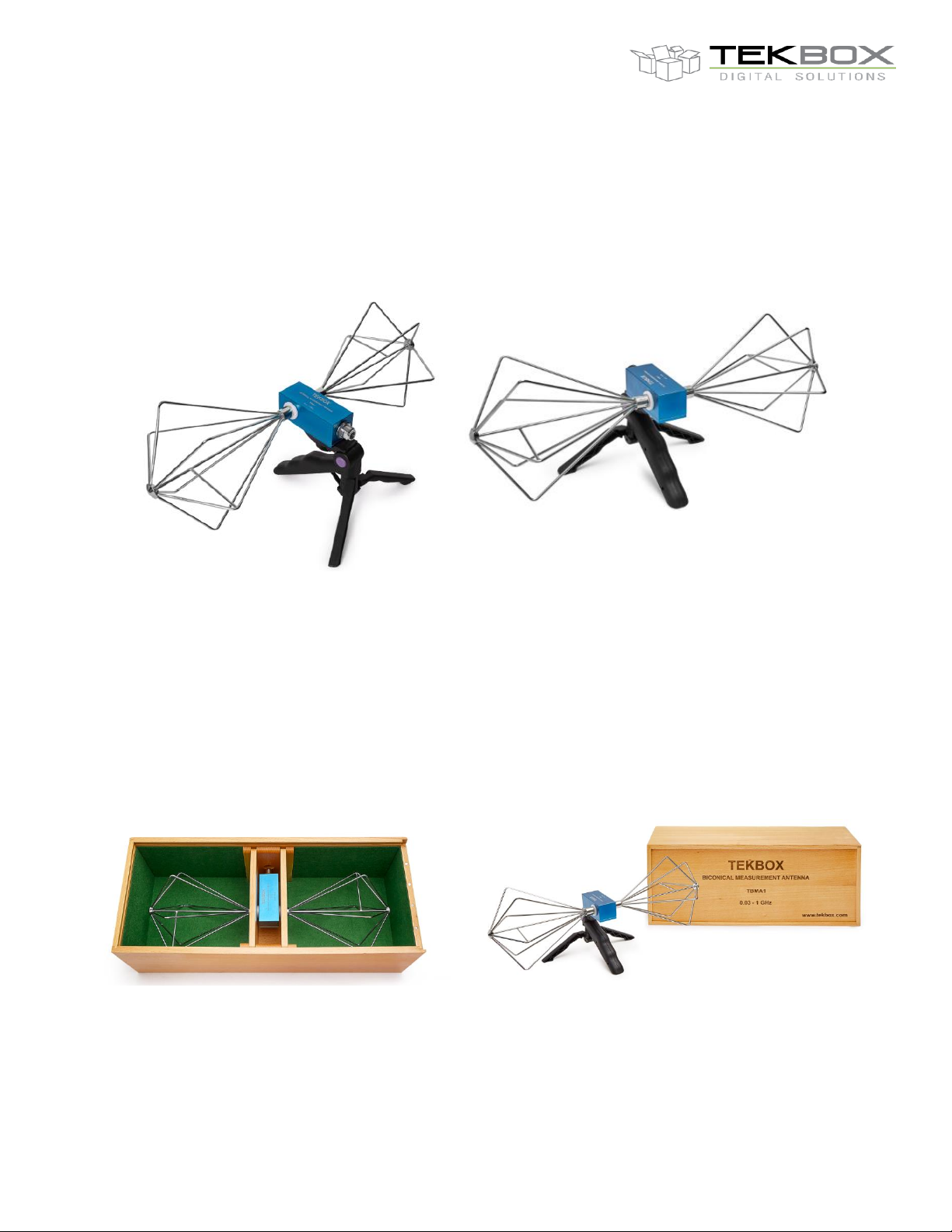
The TBMA1 is a small, lightweight, wideband biconical measurement antenna. With its moderate price, it is
targeting radiated noise EMC pre-compliance testing and generating defined field strengths.
It is characterized from 30 MHz to 1 GHz and has a directional pattern similar to a dipole.
.
2 Product overview
The TBMA1 comes in a solid beech wood case, together with a “pistol-grip” tripod. A standard ¼” thread makes it
easy to connect it to most standard tripods.
The elements are corrosion resistant and constructively locked against rotation. They are fed via a wideband balun
with 2 W power handling capability. Furthermore they are protected against build-up of static charge.
Page 2
V1.2
2
TBMA1
`
30MHz – 1000 MHz Biconical Measurement Antenna
3 Technical specifications
- Type: passive biconical
- Frequency range: 30 MHz – 1000MHz
- Nominal impedance: 50 Ω
- Maximum continuous input RF power: 2 W
- Connector: N type female
- Matching: 1:2 transformer + 1:1 balun
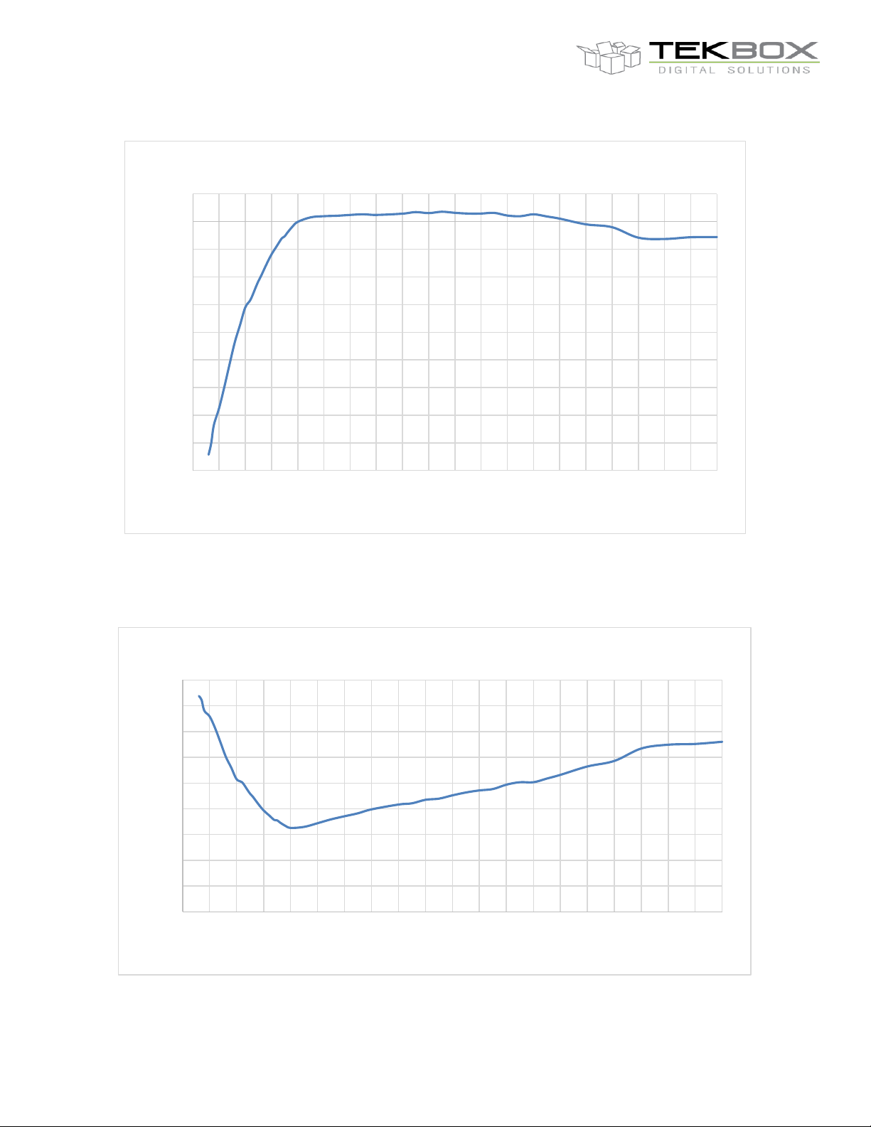
- Isotropic gain: -42.15 … 1.78 dBi
- Antenna factor: 16.30 … 41.91 dB/m
- Voltage Standing Wave Ratio (VSWR) Max < 2.8
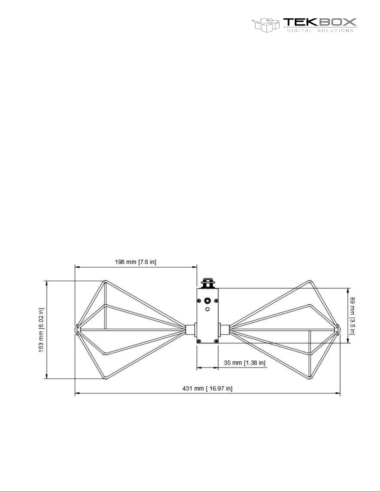
- Length: 430 mm (17 “) tip-to-tip
- Diameter: 160 mm (6.3 “)
- Depth: 163 mm (6.4 “) including housing
- Weight: 0.46 kg (1.01 lbs)
- Tripod Adapter Thread Size: ¼”
Page 3
V1.2
3
TBMA1
`
30MHz – 1000 MHz Biconical Measurement Antenna
4 RF Properties
4.1 TBMA1 Antenna characterization
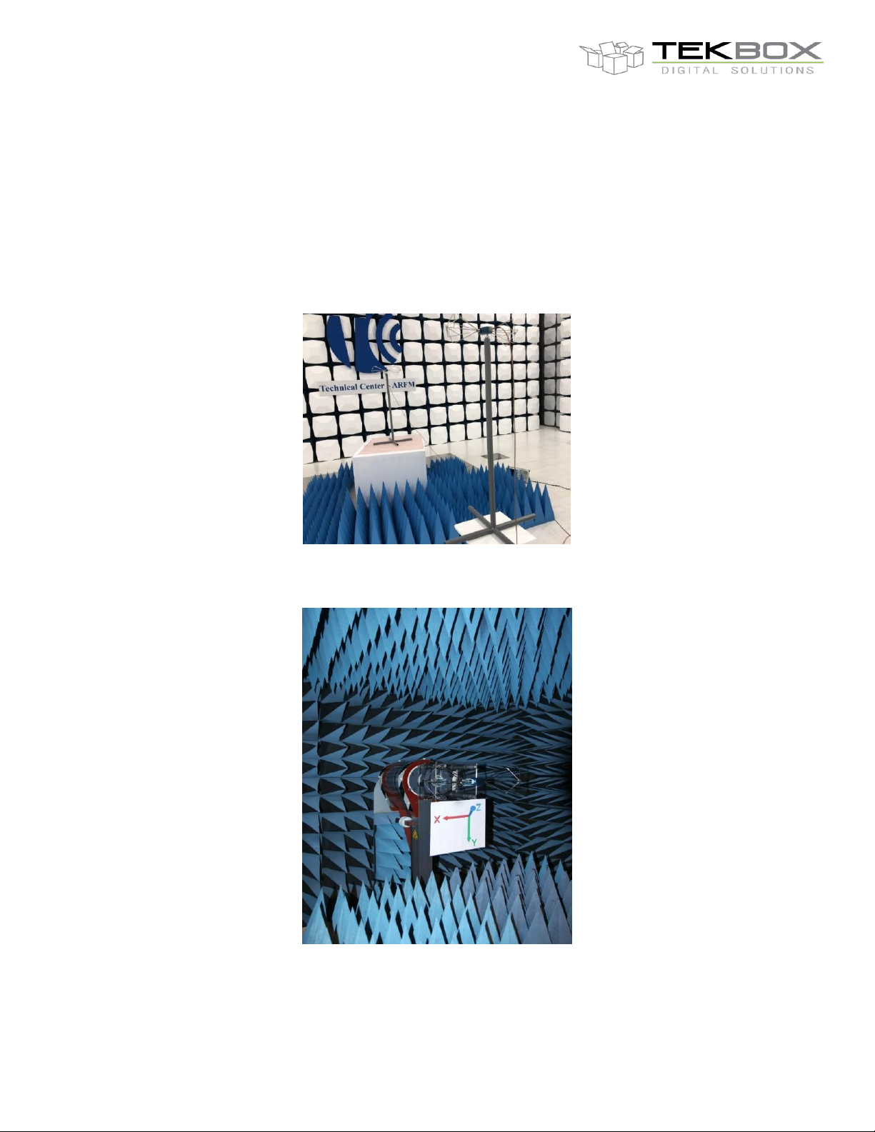
The TBMA1 has been characterized using standard calibration techniques and the results are documented in the
tables further down.
TBMA1 characterization set up inside a 10m Semi Anechoic Chamber (SAC)
TBMA1 characterization setup inside an antenna test house
Page 4

V1.2
4
Frequency
Wavelength
Gain (Isotropic)
Gain (Dipole)
Antenna Factor
MHz m dBi
dBd
dB/m
20.00
15.00
-46.76
-48.91
43.00
25.00
12.00
-44.36
-46.51
42.54
27.00
11.11
-43.46
-45.61
42.31
30.00
10.00
-42.15
-44.30
41.91
35.00
8.57
-40.06
-42.21
41.16
40.00
7.50
-36.80
-38.95
39.06
50.00
6.00
-33.74
-35.89
37.94
60.00
5.00
-29.90
-32.05
35.69
70.00
4.29
-25.79
-27.94
32.92
80.00
3.75
-21.81
-23.96
30.09
90.00
3.33
-18.69
-20.84
28.00
100.00
3.00
-15.51
-17.66
25.73
110.00
2.73
-14.13
-16.28
25.18
120.00
2.50
-11.87
-14.02
23.67
125.00
2.40
-10.77
-12.92
22.93
130.00
2.31
-9.86
-12.01
22.35
140.00
2.14
-7.81
-9.96
20.95
150.00
2.00
-5.94
-8.09
19.69
160.00
1.88
-4.45
-6.60
18.75
170.00
1.76
-2.98
-5.13
17.81
175.00
1.71
-2.69
-4.84
17.77
180.00
1.67
-2.04
-4.19
17.37
190.00
1.58
-0.91
-3.06
16.71
200.00
1.50
-0.06
-2.21
16.30
225.00
1.33
0.77
-1.38
16.49
250.00
1.20
0.97
-1.18
17.21
275.00
1.09
1.05
-1.10
17.96
300.00
1.00
1.20
-0.95
18.56
325.00
0.92
1.32
-0.83
19.14
350.00
0.86
1.21
-0.94
19.90
400.00
0.75
1.43
-0.72
20.83
425.00
0.71
1.72
-0.43
21.07
450.00
0.67
1.53
-0.62
21.76
475.00
0.63
1.78
-0.37
21.98
500.00
0.60
1.58
-0.57
22.62
525.00
0.57
1.45
-0.70
23.17
550.00
0.55
1.45
-0.70
23.58
575.00
0.52
1.57
-0.58
23.84
600.00
0.50
1.09
-1.06
24.69
625.00
0.48
0.97
-1.18
25.17
650.00
0.46
1.31
-0.84
25.17
675.00
0.44
0.93
-1.22
25.88
700.00
0.43
0.53
-1.62
26.59
750.00
0.40
-0.50
-2.65
28.22
800.00
0.38
-1.02
-3.17
29.30
850.00
0.35
-2.91
-5.06
31.72
900.00
0.33
-3.15
-5.30
32.45
950.00
0.32
-2.83
-4.98
32.60
1000.00
0.30
-2.80
-4.95
33.02
TBMA1
`
4.1 Gain & Antenna Factor versus frequency
30MHz – 1000 MHz Biconical Measurement Antenna
Page 5
V1.2
5
-45
-40
-35
-30
-25
-20
-15
-10
-5
0
5
0 50 100 150 200 250 300 350 400 450 500 550 600 650 700 750 800 850 900 950 1000
Isotropic Gain [dBi]
Frequency [MHz]
Isotropic Gain
0
5
10
15
20
25
30
35
40
45
0 50 100 150 200 250 300 350 400 450 500 550 600 650 700 750 800 850 900 950 1000
Antenna Factor [dB/m]
Frequency [MHz]
Antenna Factor
TBMA1
`
30MHz – 1000 MHz Biconical Measurement Antenna
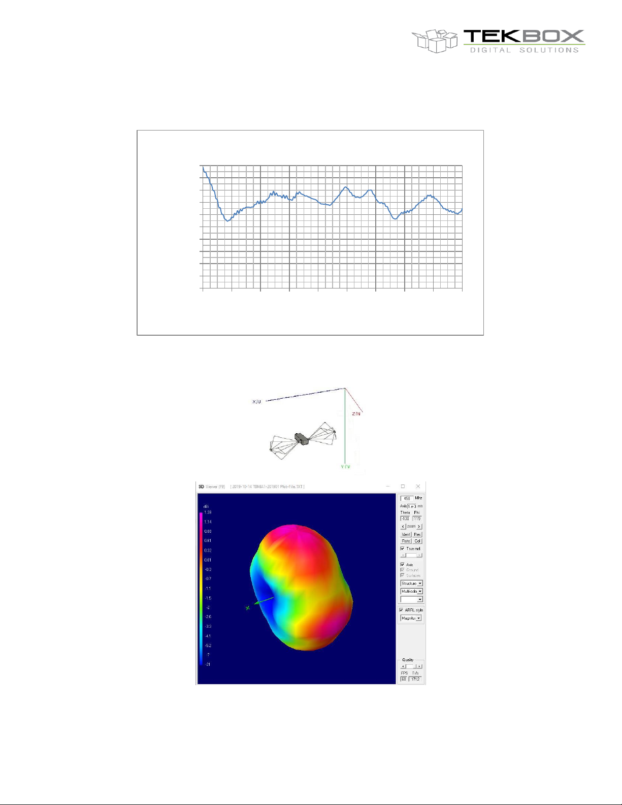
30 MHz…1 GHz , Isotropic Gain of TBMA1
30 MHz…1 GHz , Antenna Factor of TBMA1
Page 6
V1.2
6
0.00
10.00
20.00
30.00
40.00
50.00
60.00
70.00
80.00
90.00
100.00
300 400 500 600 700 800 900 1000 1100 1200
dBi
MHz
Radiation Efficiency in %
TBMA1
`
30MHz – 1000 MHz Biconical Measurement Antenna
300MHz…1200MHz , TBMA1 Radiation Efficiency
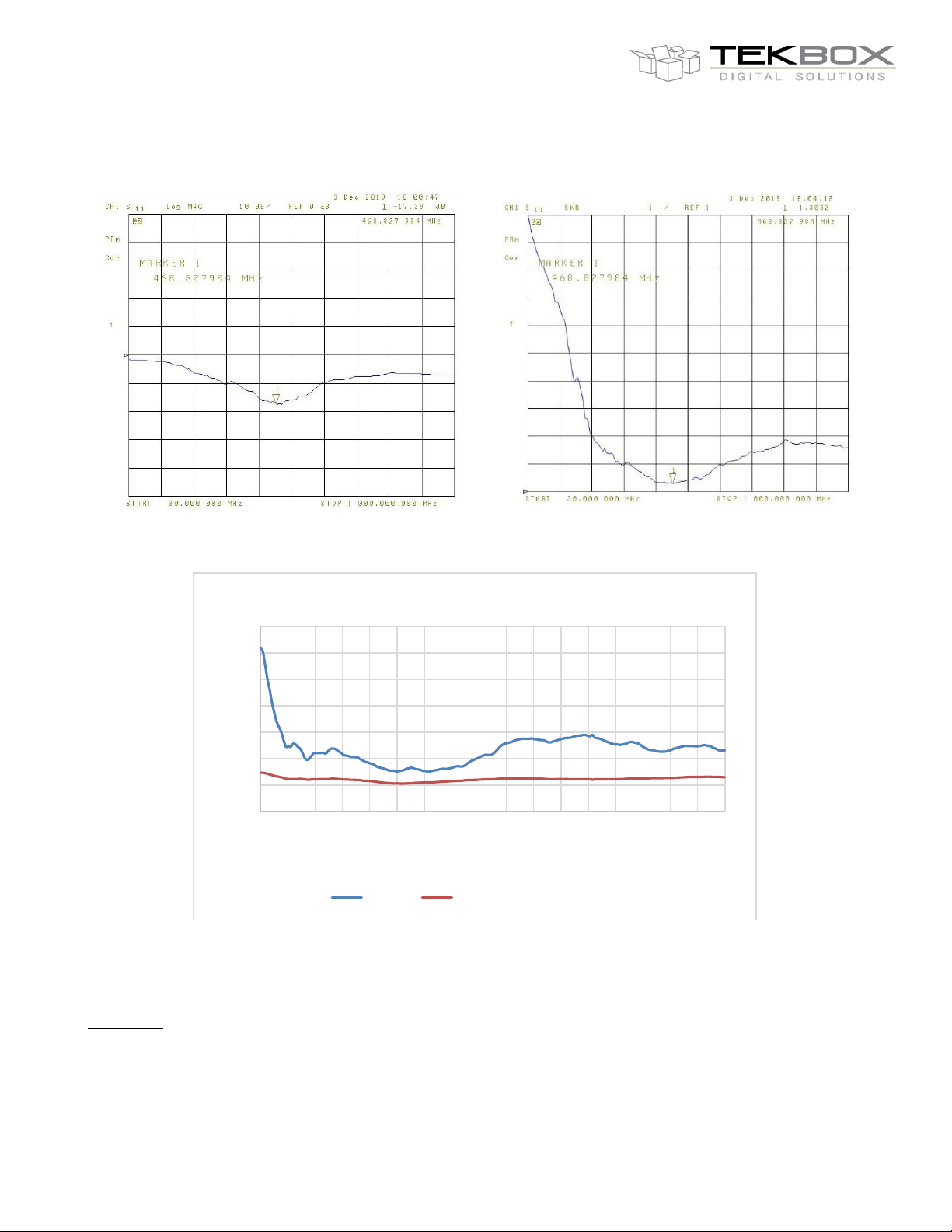
radiation pattern of the TBMA1 at 450 MHz
Page 7
V1.2
7
0
1
2
3
4
5
6
7
150 200 250 300 350 400 450 500 550 600 650 700 750 800 850 900 950 1000
VSWR at N Connector
Frequency [MHz]
TBMA1 VSWR
VSWR VSWR (With 6 dB Attenuator)
via 6 dB Attenuator
TBMA1
`
30MHz – 1000 MHz Biconical Measurement Antenna
4.2 TBMA1 Return Loss / VSWR
TBMA1, S11, 30 MHz…1 GHz TBMA1, VSWR, 30 MHz…1 GHz
Symmetry: At frequencies below 60 MHz, the TBMA1 becomes slightly asymmetric. This is not relevant in
horizontal orientation. When using the antenna in vertical orientation, position the antenna so that the engraved
text on the housing is oriented reversed / upside down.
VSWR without/ with 6 dB Attenuator
Page 8

V1.2
8
Conversion 1 m to 3 m
subtract 9.5 dB
Conversion 1 m to 10 m
subtract 20 dB
Conversion 2 m to 3 m
subtract 3.5 dB
Conversion 2 m to 10 m
subtract 14 dB
Conversion 3 m to 10 m
subtract 10.5 dB
TBMA1
`
30MHz – 1000 MHz Biconical Measurement Antenna
5 Application
The TBMA1 was designed, targeting radiated noise EMC pre-compliance measurements.
To make optimum use of the TBMA1, a few details need to be considered:
The TBMA1 does not contain any filters at the output port. Consequently, high amplitude signals that appear at
the RF output, especially when employing external pre-amplifiers might overdrive the spectrum analyzer and the
resulting intermodulation will cause measurement errors. In environments with high ambient noise levels, using
suitable filters may be of advantage.
The ambient noise level picked up by the antenna in an unshielded environment, combined with the base noise
level of the analyzer may already cross the radiated emission limits of certain CISPR standards, even with no DUT
present. Consequently, it may be very difficult to differentiate ambient noise and radiated noise from the DUT in
an unshielded environment.
Even turning ON/OFF the DUT to identify the radiated noise from the DUT may often not be a solution, given the
dynamic characteristics of contemporary sources of ambient noise.
A suitable procedure is first measuring the radiated noise of the DUT in a TEM cell which is placed in a shielded
tent or shielded bag. This will give an excellent overview of the emitted noise spectrum of the DUT. You can easily
identify the strongest emissions of the DUT and thereafter re-measure it in an open area test site (OATS) with the
measurement antenna. You then don´t need to confuse yourself with the entire ambient spectrum. Simply set the
center frequency of the analyzer to the critical emission frequencies of the DUT, one by one. Choose a span as
narrow as possible to zoom only at the frequency of the investigated DUT spurious. In case that the base noise is
still too high, you can use suitable external bandpass filters, reduce the resolution bandwidth of the analyzer or
move the antenna closer to the DUT until you can clearly identify the DUT spurious and measure its level. As long
as you keep your antenna in the far field, you can easily convert from the actual measurement distance to the
equivalent level in 3m or 10m distance.
In case that the DUT spurious exceed the limit of the standard, take it back to your lab and use near field probes
to locate the origin of the spurious on your DUT PCBA. Take suitable measures to reduce the emissions of your
product. Track the effect of the modifications by TEM cell measurements, until the relative improvement measured
in the TEM cell matches the relative improvement required to meet the far field limits according to the relevant
standard.
Then carry out another OATS measurement of the DUT to validate, if the DUT´s radiated emissions are within the
limits when measured with an antenna.
Use following formula to convert the measurement result from the actual measurement distance to the distance
specified in the relevant standard:
where is the actual measurement distance and is the specified distance in the relevant standard.
is the RF power measured in the actual measurement distance.
represents the calculated equivalent RF power in the distance specified in the relevant standard.
Alternatively use the conversion table below:
[dBm]
Page 9

V1.2
9
Frequency
Wavelength
Reactive Near Field Region
Radiative Near Field Region
Transition Zone
Far Field region
MHz m m m m
m
20.00
15.00
<2.39
2.39 – 15.00
15.00 – 30.00
>30.00
25.00
12.00
<1.91
1.91 – 12.00
12.00 – 24.00
>24.00
27.00
11.11
<1.77
1.77 – 11.11
11.11 – 22.22
>22.22
30.00
10.00
<1.59
1.59 – 10.00
10.00 – 20.00
>20.00
35.00
8.57
<1.36
1.36 – 8.57
8.57 – 17.14
>17.14
40.00
7.50
<1.19
1.19 – 7.50
7.50 – 15.00
>15.00
50.00
6.00
<0.95
0.95 – 6.00
6.00 – 12.00
>12.00
60.00
5.00
<0.80
0.80 – 5.00
5.00 – 10.00
>10.00
70.00
4.29
<0.68
0.68 – 4.29
4.29 – 8.58
>8.58
80.00
3.75
<0.60
0.60 – 3.75
3.75 – 7.5
>7.5
90.00
3.33
<0.53
0.53 – 3.33
3.33 – 6.66
>6.66
100.00
3.00
<0.48
0.48 – 3.00
3.00 – 6.00
>6.00
110.00
2.73
<0.43
0.43 – 2.73
2.73 – 5.46
>5.46
120.00
2.50
<0.40
0.40 – 2.50
2.50 – 5.00
>5.00
125.00
2.40
<0.38
0.38 – 2.40
2.40 – 4.80
>4.80
130.00
2.31
<0.37
0.37 – 2.31
2.31 – 4.62
>4.62
140.00
2.14
<0.34
0.34 – 2.14
2.14 – 4.28
>4.28
150.00
2.00
<0.32
0.32 – 2.00
2.00 – 4.00
>4.00
160.00
1.88
<0.30
0.30 – 1.88
1.88 – 3.76
>3.76
170.00
1.76
<0.28
0.28 – 1.76
1.76 – 3.52
>3.52
175.00
1.71
<0.27
0.27 – 1.71
1.71 – 3.42
>3.42
180.00
1.67
<0.27
0.27 – 1.67
1.67 – 3.34
>3.34
190.00
1.58
<0.25
0.25 – 1.58
1.58 – 3.16
>3.16
200.00
1.50
<0.24
0.24 – 1.50
1.50 – 3.00
>3.00
225.00
1.33
<0.21
0.21 – 1.33
1.33 – 2.66
>2.66
250.00
1.20
<0.19
0.19 – 1.20
1.20 – 2.40
>2.40
275.00
1.09
<0.17
0.17 – 1.09
1.09 – 2.18
>2.18
300.00
1.00
<0.16
0.16 – 1.00
1.00 – 2.00
>2.00
325.00
0.92
<0.15
0.15 – 0.92
0.92 – 1.84
>1.84
350.00
0.86
<0.14
0.14 – 0.43
0.43 – 0.86
>0.86
400.00
0.75
<0.12
0.12 – 0.49
0.49 – 0.75
>0.75
425.00
0.71
<0.11
0.11 – 0.52
0.52 – 0.71
>0.71
450.00
0.67
<0.11
0.11 – 0.55
0.55 – 0.67
>0.67
475.00
0.63
<0.10
0.10 – 0.59
0.59 – 0.63
>0.63
500.00
0.60
<0.10
0.10 – 0.60
0.60 – 0.62
>0.62
525.00
0.57
<0.09
0.09 – 0.57
0.57 – 0.65
>0.65
550.00
0.55
<0.09
0.09 – 0.55
0.55 – 0.67
>0.67
575.00
0.52
<0.08
0.08 – 0.52
0.52 – 0.71
>0.71
600.00
0.50
<0.08
0.08 – 0.50
0.50 – 0.74
>0.74
625.00
0.48
<0.08
0.08 – 0.48
0.48 – 0.77
>0.77
650.00
0.46
<0.07
0.07 – 0.46
0.46 – 0.81
>0.81
675.00
0.44
<0.07
0.07 – 0.44
0.44 – 0.84
>0.84
700.00
0.43
<0.07
0.07 – 0.43
0.43 – 0.86
>0.86
750.00
0.40
<0.06
0.06 – 0.40
0.40 – 0.93
>0.93
800.00
0.38
<0.06
0.06 – 0.38
0.38 – 0.98
>0.98
TBMA1
`
30MHz – 1000 MHz Biconical Measurement Antenna
However, when applying the conversions above, be aware, that even in the set up specified in the standards, the
measurement antenna is not in the far field across the entire frequency range. This would physically be impossible,
given the size limitations of anechoic chambers.
The following table gives an overview of the near field and far field distances from TBMA1 depending on frequency.
As an example, assuming an actual measurement distance of 1 m, the above conversions would become valid at
frequencies above 350 MHz.
Page 10
V1.2
10
850.00
0.35
<0.06
0.06 – 0.35
0.35 – 1.06
>1.06
900.00
0.33
<0.05
0.05 – 0.33
0.33 – 1.12
>1.12
950.00
0.32
<0.05
0.05 – 0.32
0.32 – 1.16
>1.16
1000.00
0.30
<0.05
0.05 – 0.30
0.30 – 1.24
>1.24
Part Number
Description
TBMA1
30 MHz – 1 GHz biconical measurement antenna, mini tripod, wooden box
Version
Date
Author
Changes
V1.0
13.1.2020
Mayerhofer
Creation of the document
V1.1
17.1.2020
Gharachorloo
Updated in chapter 3
V1.2
17.6.2020
Mayerhofer
Chapter 3: information on matching
Chapter 4: information on symmetry
TBMA1
`
30MHz – 1000 MHz Biconical Measurement Antenna
Note that the discontinuity in the above table between 325 MHz and 350 MHz originates from applying two models.
The first model applies for antennas physically shorter than half of the wavelength and the second model applies
for antennas physically longer than half of the wavelength. Obviously, the formulas for the two models do not
smoothly transit into each other.
6 Ordering Information
7 History
 Loading...