

Page 1
Tekbox EMCview Manual_V2_2.docx V2.2
Tekbox EMCview Manual
Contents
1. Introduction ........................................................................................................................................................... 2
2. Installation ............................................................................................................................................................. 2
3. Warning – spectrum analyzer input rating ............................................................................................................ 2
4. Projects .................................................................................................................................................................. 3
5. Workspace ............................................................................................................................................................. 4
6. Connecting to the spectrum analyzer .................................................................................................................... 4
7. Prepare measurements ........................................................................................................................................... 5
8. Measurement ......................................................................................................................................................... 6
9. SRC folder - General ............................................................................................................................................. 6
10. SRC folder – Limit files ........................................................................................................................................ 7
11. SRC folder - Segments ................................ ................................ ................................................................ .......... 9
12. SRC folder – compensation files ......................................................................................................................... 11
13. SRC folder – project files .................................................................................................................................... 12
14. Peak scan ............................................................................................................................................................. 12
15. Final scan / peak re-measurement ....................................................................................................................... 13
16. View / hide graphs .............................................................................................................................................. 15
17. Zoom graphs........................................................................................................................................................ 16
18. Amplitude units ................................................................................................................................ ................... 16
19. Markers ............................................................................................................................................................... 16
20. Labels .................................................................................................................................................................. 18
21. Options ................................................................................................................................................................ 19
22. Fader.................................................................................................................................................................... 20
23. Math .................................................................................................................................................................... 21
24. Saving graphs and measurement results .............................................................................................................. 22
25. Control of additional equipment with EMCview ................................................................................................ 23
26. Using RF current probe measurements to extrapolate to radiated E-field strength ............................................. 25
27. Create Reports ..................................................................................................................................................... 25
28. Tracking generator control mode for immunity testing ....................................................................................... 26
29. RF coverage measurement mode ........................................................................................................................ 26
29.1 Configuration .............................................................................................................................................. 27
29.2 Status and measurement results .................................................................................................................. 28
29.3 Log file ....................................................................................................................................................... 28
29.4 KML file ..................................................................................................................................................... 29
30. Further information ............................................................................................................................................. 29
31. History ................................................................................................................................................................. 29
Author: Mayerhofer 1 of 29 TekBox Digital Solutions 4-Nov-21
Page 2

Tekbox EMCview Manual_V2_2.docx V2.2
Tekbox EMCview Manual
1. Introduction
The EMCview software carries out automated conducted or radiated noise measurements. It currently
supports all Rigol DSA and RSA spectrum analyzers, all Siglent SSA, SSA-plus, SVA models, Rohde &
Schwarz FPC and FPH series analyzers, OWON XSA and HSA series, BK Precision models 2682/2683 and
Teledyne LeCroy T3SA series. All relevant CISPR (= EN550xx) conducted and radiated noise measurement
settings are pre-configured in the current version.
EMCview also supports RF-coverage measurements and tracking generator control for immunity testing.
This manual reflects the state of EMCview V8.0. Some screenshots may be based on older SW versions
and slightly differ from the latest versions. As EMCview is a very dynamic project, have a look at our website
from time to time for new releases with new features. As the manual is only updated for each major release,
refer to the readme files and the EMCview FAQ document for more detailed information on features.
2. Installation
Download and install the VISA driver package from the National Instruments website.
Create a directory into which you copy EMCview.exe. Execute EMCview.exe to install the software. Copy the
license file into the same directory as EMCview.exe. Click EMCview.exe within your program directory to run
the program.
Important:
Rigol DSA815 FW >= V00.01.16; Siglent SSA FW >= 1.2.9.3a; Siglent SVA FW >= V2.2.1.2.1 or higher
R&S FPC1500: >= FW 1.5 PC-requirements: Windows 7, 8, 10; min 4MB RAM
R&S FPC and FPH spectrum analyzers: In addition, install “R&S Instrumentview”. Connect over USB cable
with “SA TCP” = 172.16.10.10. Connection over LAN is not recommended, as it works very slowly.
In case of an update, in order to get any new project files updated as well, you need to delete the SRC folder
of the installation directory. Else the SRC folder will not be updated to protect customer made or modified
projects from being deleted or overwritten. Alternatively, install new versions in another directory, e.g.
C:\EMCview_New\.
If you want to re-size the main window, pull it with your mouse to fit it to the size of your display.
Limitation without license: The upper frequency of measurements is limited to 10MHz
Execute EMCview with parameter s, if you have a tiny display and need scrollbars.
3. Warning – spectrum analyzer input rating
Always consider the maximum input ratings of any spectrum analyzer. Be aware that powerful
surges and harmonics of a DUT may have the potential to damage the spectrum analyzer input
stage.
Be aware, that EMCview project files are set up to utilize the maximum sensitivity of the spectrum analyzer.
The requirements of certain standards are tough, especially those of CISPR 25 class 5 and manufacturer
specific automotive conducted noise standards. Consequently, the internal attenuator is set to OFF and the
internal preamplifier is set to ON in order to avoid crossing the limit lines with the noise level of the analyzer.
Furthermore, all conductive noise measurement projects use the LISN correction file for disabled
attenuator/limiter.
Take following precautions to protect the spectrum analyzer input before testing an
unknown DUT:
Check the attenuator and preamplifier settings of the segment file upfront to any measurement
Be especially careful when testing conducted emissions of inductive loads such as motors or switched
inductive loads.
Whenever measuring an unknown source or DUT, protect the spectrum analyzer input with the internal
limiter an external attenuator of 20dB or 30dB and check the spectrum for any high amplitude signals.
Protect the spectrum analyzer input from harmful ESD events.
In case of conducted noise measurements with the 50µH LISN (TBLC08) follow the procedure in the LISN
manual. With the LISN power switch OFF, the line selection switch OFF and the LISN attenuator/limiter on,
first power the isolation transformer and thereafter turn ON the LISN power switch. Next, connect the
powered spectrum analyzer via BNC cable to the LISN. The internal spectrum analyzer attenuator shall be
Author: Mayerhofer 2 of 29 TekBox Digital Solutions 4-Nov-21
Page 3
Tekbox EMCview Manual_V2_2.docx V2.2
Tekbox EMCview Manual
ON and the internal preamplifier shall be OFF. It is a good practice to keep the spectrum analyzer RF input
disconnected or at least the line switch in OFF position when powering ON/OFF the DUT in order to protect
the analyzer from potentially harmful switching transients.
In case of the 5µH LISN (TBOH01) use an external 20dB attenuator or consider using an external limiter
such as the TBFL1 for a first check.
Before running a test with EMCview, monitor especially the frequency range 9 kHz to 2 MHz for potential
high amplitude harmonics and check for spectrum analyzer messages “IF overload”. Operate the spectrum
analyzer with Max Hold for this purpose. In case of strong signals, increase the attenuator and reference
Level of the analyzer or even add an external attenuator at the input.
Modify the segment file with respect to attenuator and preamplifier settings accordingly. When doing
a fast scan, consider the attenuator and preamplifier settings in the control box.
Hint: attenuator and preamplifier settings in the segment files can easily be modified using a text editor with
“find and replace all” capability.
4. Projects
In EMCview, any EMC standard is represented by one or more projects. A project summarizes all
configurations necessary to carry out measurements. It consists of limit files, segment files, a cable file, a
LISN file, an antenna file, an amplifier file and various settings such as graph boundaries, trace colors, and
settings for peak measurements.
Limit files: configuration containing the frequency dependent limit values given in the corresponding
standard.
Segment files: spectrum analyzer settings such as start and stop frequency, sweep time, resolution
bandwidth, detector, attenuator and preamplifier settings. Refer to the CISPR16 standard or to the Tekbox
document Pre Compliance Conducted Emission Measurements V1_1.pdf for more detailed information.
Radiated noise measurements often cover a wide frequency span and require different antennas for
different frequency ranges. Consequently, it makes sense to split segment files. Segment files for radiated
noise typically cover 150kHz -30MHz, 30MHz-300MHz, 300MHz-1GHz, 1GHz – 1,5GHz (DSA815 frequency
range), etc.
LISN files: insertion loss/calibration data of the LISN over frequency, entered in dB with negative sign. Use
LISN files also to implement conversion from dBµV to dBµA for conducted noise measurements with RF
current probes. The default 50µH LISN file is using the correction data for the attenuator/limiter in OFF
position. If you measure with attenuator/limiter engaged, select the corresponding LISN file.
Antenna files: antenna factor of the antennas used for radiated noise measurement; converts the dBµV
measured by the spectrum analyzer into dBµV/m
Cable files: insertion loss of cables between DUT and spectrum analyzer
Gain files: amplifier gain or attenuator loss in the signal path, if any
These files can be created or edited either with a built in editor in the Setup Menu or with any text editor.
The files are located in the src subdirectory. Press the Tab key after loading any configuration file.
Project files for conducted noise measurements have file names starting with CN_*.prj. Project files for
radiated noise measurements with antennas start with RN_*.prj. Project files for radiated noise
measurements with TEM cells start with TC_*.prj.
Refer to the applicable standards for more details and insight. Standards and corresponding limits may
change over time. Tekbox does not take any liability for the validity of the limits and other settings in the
preconfigured projects.
Consider that most segment files have the default attenuator settings at 0dB and in some cases such as
CISPR 25 the preamplifier of the spectrum analyzer is set to ON in order to achieve maximum sensitivity.
When testing any device with switched mode power supplies, consider to change the attenuator setting to
10dB for the first run.
Also in case of an “IF Overload” message of the analyzer, stop the measurement and disconnect the
analyzer and increase the attenuator setting before proceeding with the measurement.
Author: Mayerhofer 3 of 29 TekBox Digital Solutions 4-Nov-21
Page 4
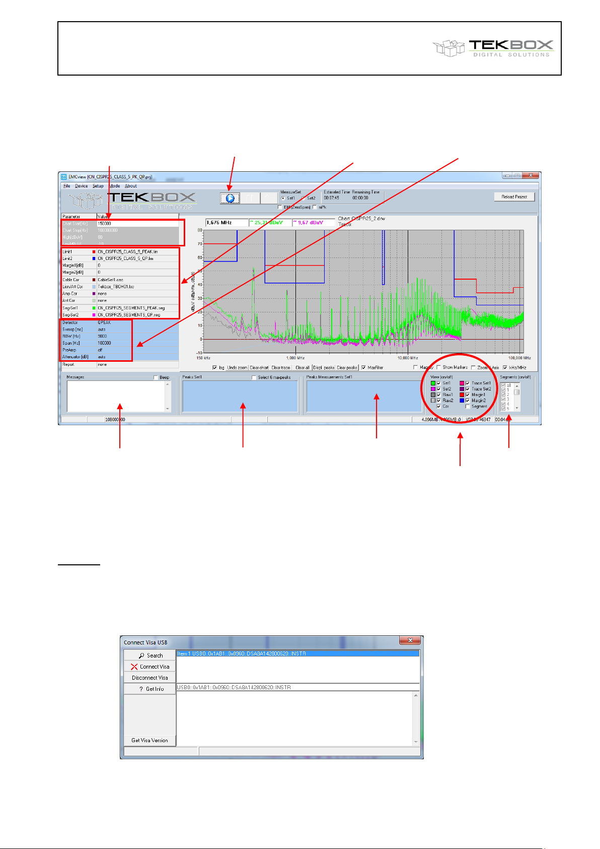
Tekbox EMCview Manual_V2_2.docx V2.2
Set chart axis boundaries
/ zoom
Settings for the peak remeasurement (final scan)*
measurement
configuration files
Notifications /warnings /
error messages
Re-measures selected peaks
lists peaks which violate the
margin of the limit line
view / hide traces
Start / pause / stop
measurement
selective measurement
of segments
Tekbox EMCview Manual
5. Workspace
* With EMCview V8.0, peak re-measurement UI was simplified and settings reduced to the drift span
6. Connecting to the spectrum analyzer
Via USB: Launch EMCview and connect the spectrum analyzer to the PC via USB.
In the menu line, click DEVICE, then DSA USB and SEARCH. You should then see the Rigol analyzer listed
in the search window. Click at the line with the Rigol Analyzer and then click the CONNECT VISA button. You
can validate the connection by clicking the GET INFO button. Furthermore, you should see a “licensed” status
message in the very left lower corner of EMCview. Close the window with the x button. Do not close it with the
Disconnect Visa button, as it would disconnect the spectrum analyzer.
Author: Mayerhofer 4 of 29 TekBox Digital Solutions 4-Nov-21
limits or which are within a set
using other settings – e.g. quasi
peak detektor measurement
of peaks detected during a
measurement of „Set1“
Page 5
Tekbox EMCview Manual_V2_2.docx V2.2
Tekbox EMCview Manual
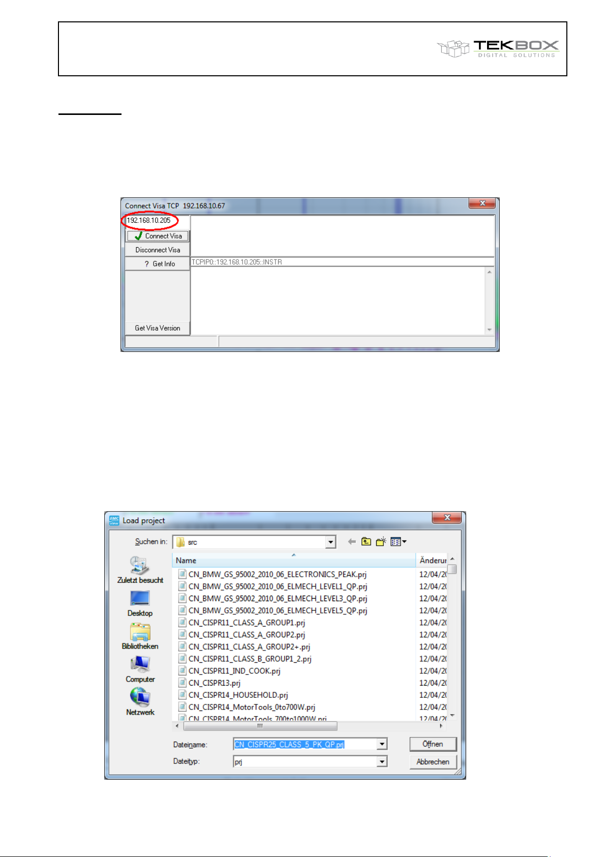
Via Ethernet: Launch EMCview and connect the spectrum analyzer to the PC via an Ethernet cable. On the
analyzer LAN settings, change to manual IP and enter an IP address, e.g. 192.168.10.205
In the menu line, click DEVICE, then DSA TCP. Enter the IP address of the spectrum analyzer into the box at
the upper right corner. Click the CONNECT VISA button. You can validate the connection by clicking the GET
INFO button. Furthermore, you should see a “licensed” status message in the very left lower corner of
EMCview. Close the window with the x button. Do not close it with the Disconnect Visa button, as it would
disconnect the spectrum analyzer.
7. Prepare measurements
Click File, Load Project and select an appropriate standard for your DUT.
The predefined limit lines and segment files for the selected standard will pop up in the box at the left side of
the window. The limit lines will appear in the graph chart.
If you miss any standard, you can create new limit lines, segment files and correction files in the menu Setup.
Alternatively and most likely the faster approach, you can copy, rename and modify one of the existing files
using a text editor.
Author: Mayerhofer 5 of 29 TekBox Digital Solutions 4-Nov-21
Page 6
Tekbox EMCview Manual_V2_2.docx V2.2
Tekbox EMCview Manual
If you change to any other configuration file during an ongoing session with EMCview, press the Reload
Project files button in the right upper corner.
8. Measurement
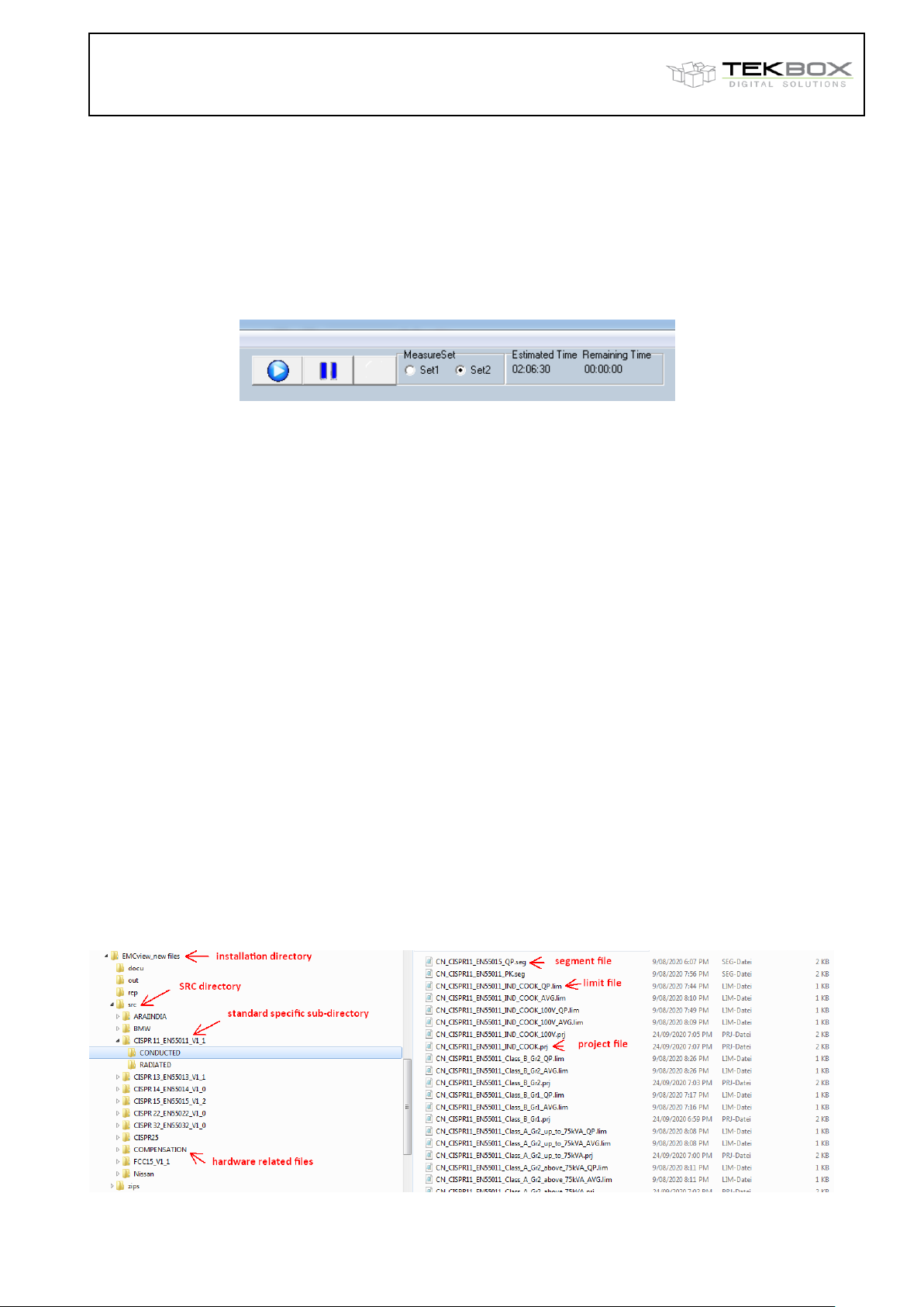
After correct set up and configuration, just press the Play button at the top of the window. The analyzer will
start carrying out the measurement defined in Segment-Set 1. The associated limit line is Limit1. After the
measurement is completed, click the Set2 button at the top of the window. Press the Play button. The analyzer
will start carrying out the measurement defined in Segment-Set 2. The associated limit line is Limit2.
Most project files define Peak or Average measurements as Set1 and Quasi-Peak measurements as Set2.
By default, all segments are measured and displayed consecutively.
9. SRC folder - General
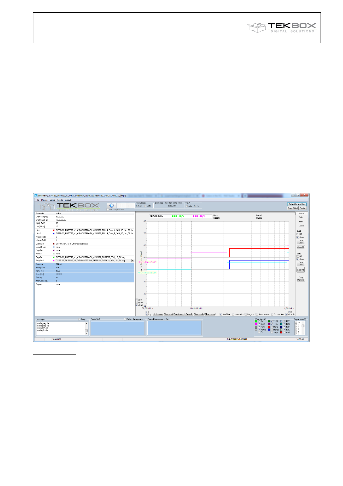
The SRC – folder is a sub directory of the installation directory of EMCview. The SRC folder contains:
Project files, which
define graph boundaries – start frequency, stop frequency, minimum amplitude, maximum amplitude
reference limit line files – conducted emission limits, radiated emission limits as per relevant
standard
reference segment files – spectrum analyzer parameters such as start frequency, stop frequency,
RBW, detector, sweep time, internal attenuation, pre-amplifier setting
define settings for peak re-measurement
Limit files, which then are loaded and displayed on the graph
Segment files, which control the spectrum analyzer settings and measurement
Compensation files, which characterize hardware such as LISN, current probes, antennas,
amplifiers, attenuators, cables and any other devices which influence the frequency response of the
measurement set up.
Up to EMCview V7.0, the SRC folder did not contain any sub directories. With V7.0, each standard is
contained in an individual sub directory, which then contains further sub directories for conducted noise,
radiated noise and TEM cell measurements, where foreseen by the standard. There is also a separate sub
directory for compensation files. All files in the SRC folder are plain text files, which can be created or edited
with any text editor. Alternatively, the files can be created within EMCview menu SETUP, however using a
text editor is most probably a more efficient method.
Author: Mayerhofer 6 of 29 TekBox Digital Solutions 4-Nov-21
Page 7
Tekbox EMCview Manual_V2_2.docx V2.2
Tekbox EMCview Manual
It is important to understand, that the SRC folder remains untouched, when updating EMCview. This
prevents overwriting or deleting any files, which were created or modified by the user. Consequently, any
new projects, which may have been added to the updated software, will not be added during the installation
process. In order to have the SRC directory updated during a SW update, save your customized files to
another directory and then delete the SRC directory. Thereafter you can merge your customized files with
the updated SRC directory. Alternatively, create another installation directory for EMCview, such as
C:\EMCview_NEW\, etc.
10. SRC folder – Limit files
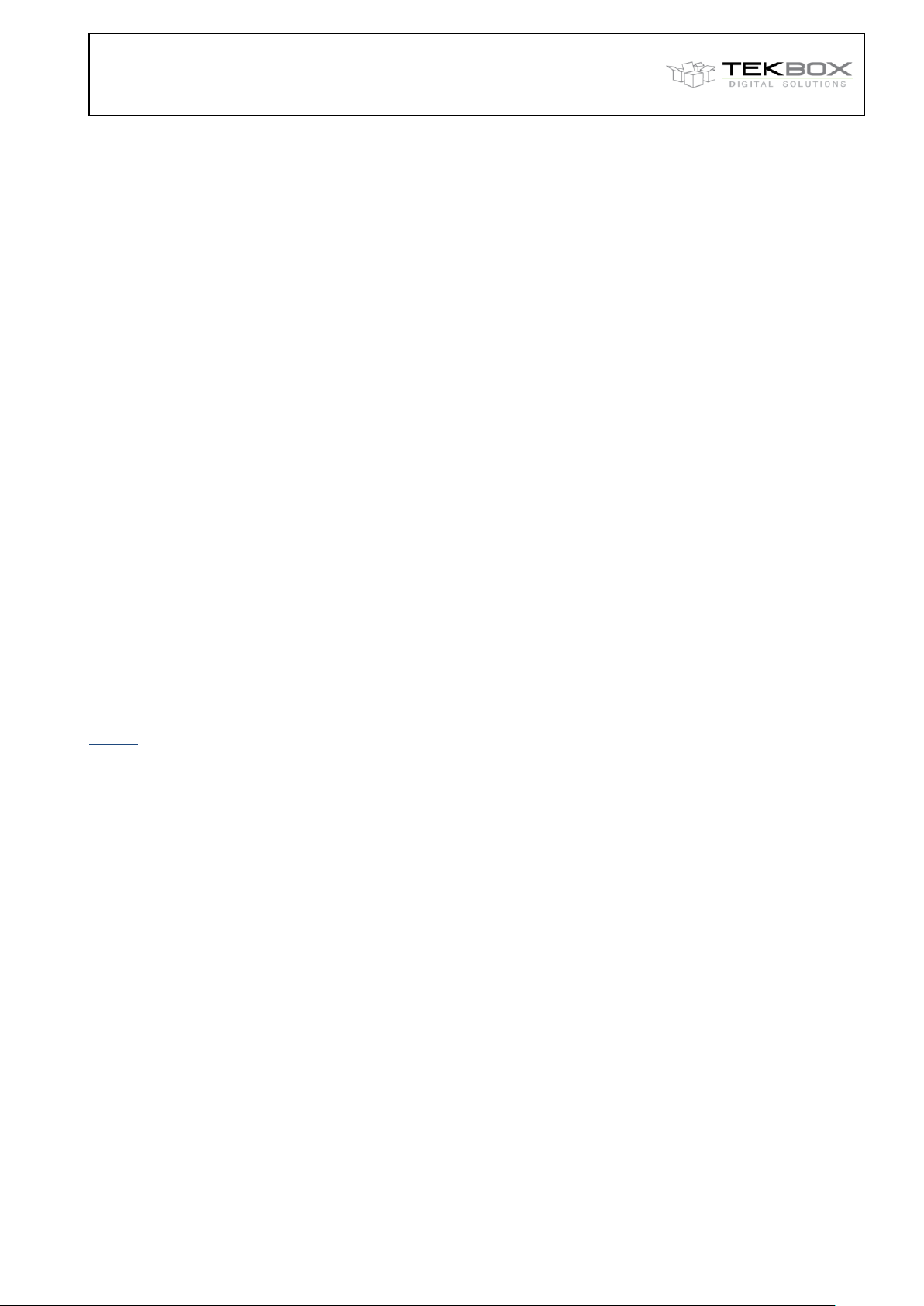
With EMCview V7.0, every limit file can contain a main limit line plus up to 15 auxiliary limit lines. In
addition, EMCview can display a margin line for each main limit line. The main limit line will be used as
reference for margin lines and to calculate peaks, which exceed the major limit line or the margin line.
Auxiliary limit lines are basically graphic content which cannot be used for any processing purpose.
Main limit lines must be coherent, whereas auxiliary limit lines can be segmented / interrupted.
Example: CISPR22 Class A and Class B as main limit lines and FCC 15 Class A and FCC 15 Class B as auxiliary
limit lines
Limit File syntax:
[Application] * start header
Software=TekBox RP-W32-D7
Version=Demo
Date=18.01.2017 09:42:29
[General]
Name=RN_CISPR22_FCC15_Class_A_30M_1G_3m_QP.lim * file name
Freq_Interplot_Mode=lin
Level_Interplot_Mode=log
[Data] * Main limit line (CISPR 22 Class A)
Freq1=30.000.000 * first frequency point [Hz]
Lev1=50.5 * amplitude level of the first frequency point [dBµV]
Freq2=230.000.000 * second frequency point
Lev2=50.5 * amplitude level of the second frequency point [dBµV]
Freq3=230.000.010 * third frequency point (using a point with 10 Hz offset
Author: Mayerhofer 7 of 29 TekBox Digital Solutions 4-Nov-21
Page 8
Tekbox EMCview Manual_V2_2.docx V2.2
Tekbox EMCview Manual
Lev3=57.5 creates a vertical step and keeps the line coherent)
Freq4=1.000.000.000
Lev4=57.5 * amplitude level of the last point of the main limit line
[Data_Limit1] * start first auxiliary limit line (FCC 15 Class A)
Caption=FCC15 Class A QP * text label for 1st auxiliary limit line
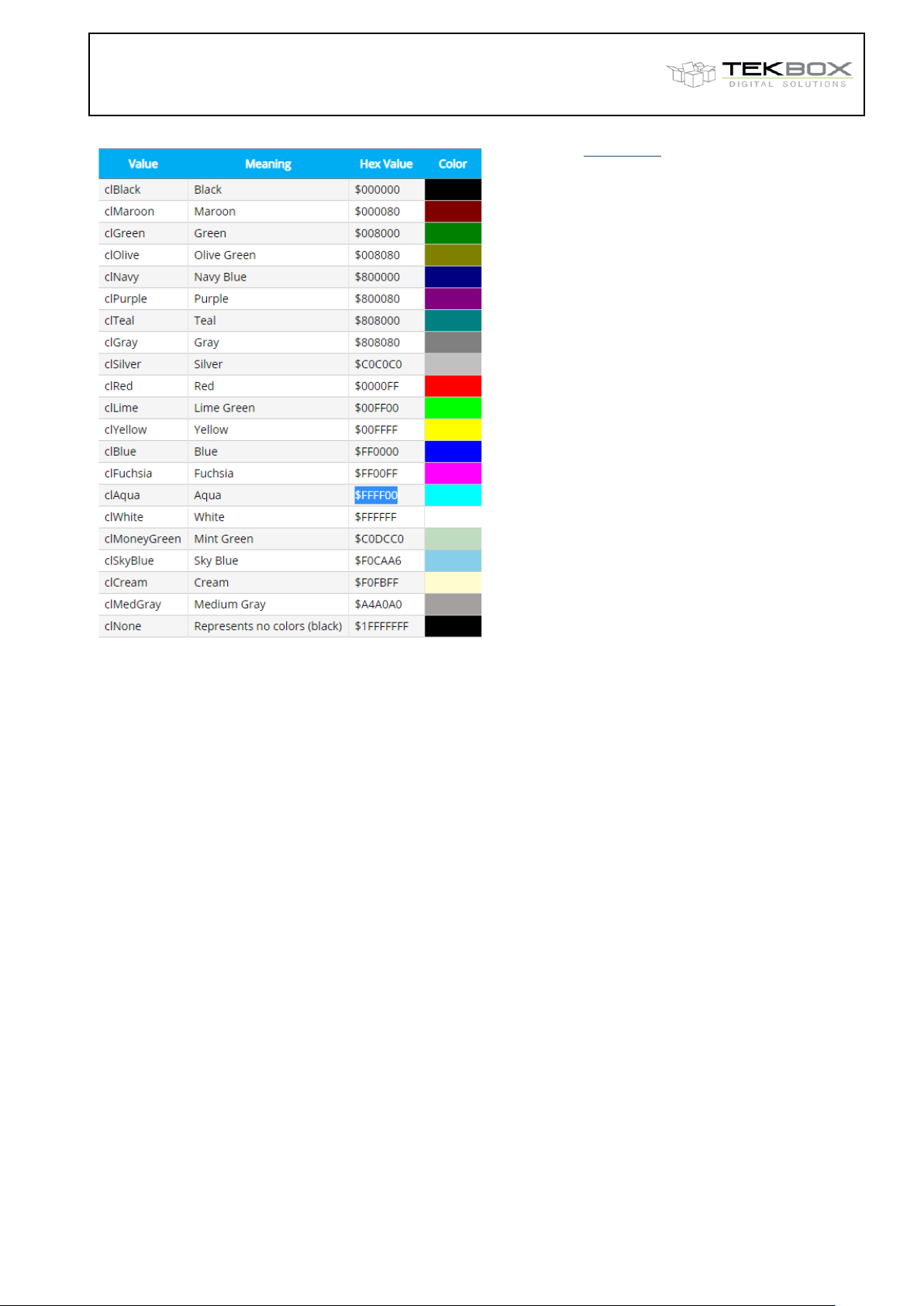
Color=$FF00FF * line color “Fuchsia” (alternatively enter clFuchsia instead of the Hex value)
Style=psSolid * line style “solid”
Freq1=30.000.000 * first frequency point of auxiliary limit line [Hz]
Lev1=49.6 * amplitude of the first frequency point of the first limit line [dBµV]
Freq2=88.000.000 * second frequency point of auxiliary limit line [Hz]
Lev2=49.6 * amplitude of the second frequency point of the first limit line [dBµV]
Break2=1 * suppress the limit line between second and third frequency point
Freq3=88.000.000 * third frequency point of auxiliary limit line [Hz]
Lev3=54
Freq4=216.000.000
Lev4=54
Break4=1
Freq5=216.000.000
Lev5=56.9
Freq6=960.000.000
Lev6=56.9
Break6=1
Freq7=960.000.000
Lev7=60
Freq8=1.000.000.000
Lev8=60 * end of 1st auxiliary limit line
[Data_Limit2] * start 2nd auxiliary limit line
Caption=enter label here * text label for auxiliary limit line
Color=$FFFF00 * line color “Aqua” (alternatively enter clAqua instead of the Hex value)
Style=psDash * line style “dashed”
Freq1=……..
……………..
Colors:
Author: Mayerhofer 8 of 29 TekBox Digital Solutions 4-Nov-21
Page 9
Tekbox EMCview Manual_V2_2.docx V2.2
Tekbox EMCview Manual
Line styles: psSolid
psDash
psDot
psDashDot
psDashDotDot
Main limit lines are usually linked to a corresponding segment file. Limit 1 is coupled with Segment Set1 and
Limit 2 is coupled with Segment Set2.
Labels of auxiliary limit lines can be moved, by dragging it with the mouse.
Interrupted main limit lines, such as specified for example in CISPR 25 are created by setting the frequency
sections without limitations to a high value such as for example 150 dBµV and thereby shifting it outside the
upper amplitude boundary of the graph window (though of course, the upper boundary could be as high or
higher than 150dBµV]. Vertical steps are created by entering two frequency points very close to each other.
Use a frequency difference of 10 Hz between the two adjacent points, for example. See Freq2 and Freq3 in
the example file above.
The default color of main limit lines can be modified in the SETUP menu. The line style is always solid.
Color and line style of auxiliary limit lines can be edited or modified inside the limit file, as shown in the
example above.
11. SRC folder - Segments
It is very important to understand the concept of segments. A segment defines a frequency sweep of the
spectrum analyzer. A segment is a piece of frequency spectrum, with a defined start frequency and a defined
stop frequency of the sweep. Segments are defined in the segment files, which are located in the src folder
of the EMCview directory. Segment files can be identified by the .seg extension. A segment file basically
defines a measurement run. The entire frequency span of the measurement run is split into many adjacent
frequency segments, means a series of frequency sweeps, which will be measured consecutively. EMCview
then stitches together the results of the individual sweeps to a single graph.
You may ask, why the entire spectrum is not measured just with a single sweep. The reason is, that a sweep
is not a continuous measurement, but a series of discrete frequency steps, at which measurements are taken.
A typical spectrum analyzer for EMC pre-compliance measurements has a display with 601 pixels in X
(frequency)-axis direction. Consequently a sweep is divided into 601 discrete frequency steps.
Author: Mayerhofer 9 of 29 TekBox Digital Solutions 4-Nov-21
Page 10
Tekbox EMCview Manual_V2_2.docx V2.2
Tekbox EMCview Manual
A consequence of this architectural detail can be seen, if you set your spectrum analyzer to full span and feed
it with a constant frequency signal, e.g. 98 MHz. Assuming a full span of 3 GHz, measurement point # 19 is
at 95 MHz and measurement point #20 is at 100 MHz. Full span resolution bandwidth typically is set to 1 MHz.
Pressing max peak at the analyzer will detect the maximum amplitude at measurement point #20 and
consequently report a peak at 100 MHz and not at 98 MHz. Worse, depending on the frequency offset of the
applied signal with respect to the nearest measurement point, it will also report a lower amplitude, as the
applied signal sits somewhere at the shoulder of the RBW filter.
To prevent incorrect measurements, CISPR 16 specifies that adjacent frequency points shall not be spaced
more than half the resolution bandwidth of the analyzer. As an example, CISPR band B, the frequency range
150 kHz to 30 MHz, must be measured with a resolution bandwidth of 9 kHz. This results in a frequency
spacing of 4.5 kHz between adjacent measurement points and a maximum sweep span of 601 * 4.5 kHz =
2.7 MHz.
Consequently, a CISPR compliant measurement can only be carried out in slices. Doing it manually would be
very inefficient and this is why automatic measurement tools such as EMCview are needed for any serious
pre-compliance tests.
Segment files of EMCview do not only define the start and stop frequencies of sweeps, but also set additional
spectrum analyzer parameters which will be associated to every single frequency segment:
Resolution Bandwidth - EMC standards specify the RBW depending on the frequency band
Sweep time – EMC standards specify the sweep time depending on RBW and detector type
Detector – EMC standards specify which detectors need to be engaged
Internal Attenuator – the internal attenuator setting effects the base noise level of the spectrum analyzer. At
the same time, the user must be aware of potentially overdriving the analyzer input and potential
intermodulation distortion which would falsify the measurement.
Internal Pre-amplifier – activating the internal pre-amplifier will lower the base noise of the analyzer. This may
be necessary for standards which have very low limits. However, similar considerations as for the internal
attenuator have to be applied.
As mentioned, segment files are located in the src folder of the EMCview directory. They are plain text files
and can be edited or created with the built in editing feature in menu Setup / Edit Segments, or perhaps more
simply and conveniently with any text editor. A segment will look as below:
FRQa__1=9.000 * segment number (#1) and start frequency (9 kHz) of the segment
FRQb__1=50.000 * segment number (#1) and stop frequency (50 kHz) of the segment
BW____1=200 * segment number (#1) and RBW (200 Hz) of the segment
Sweep_1=1000000 * segment number (#1) and sweep time (1000000 ms) of the segment
Att___1=0 * segment number (#1) and internal attenuation (0dB) of the segment
PreAmp1=off * segment number (#1) and pre amplifier setting (off) of the segment
Detector1=QPEAK * segment number (#1) and detector type (quasi peak) of the segment
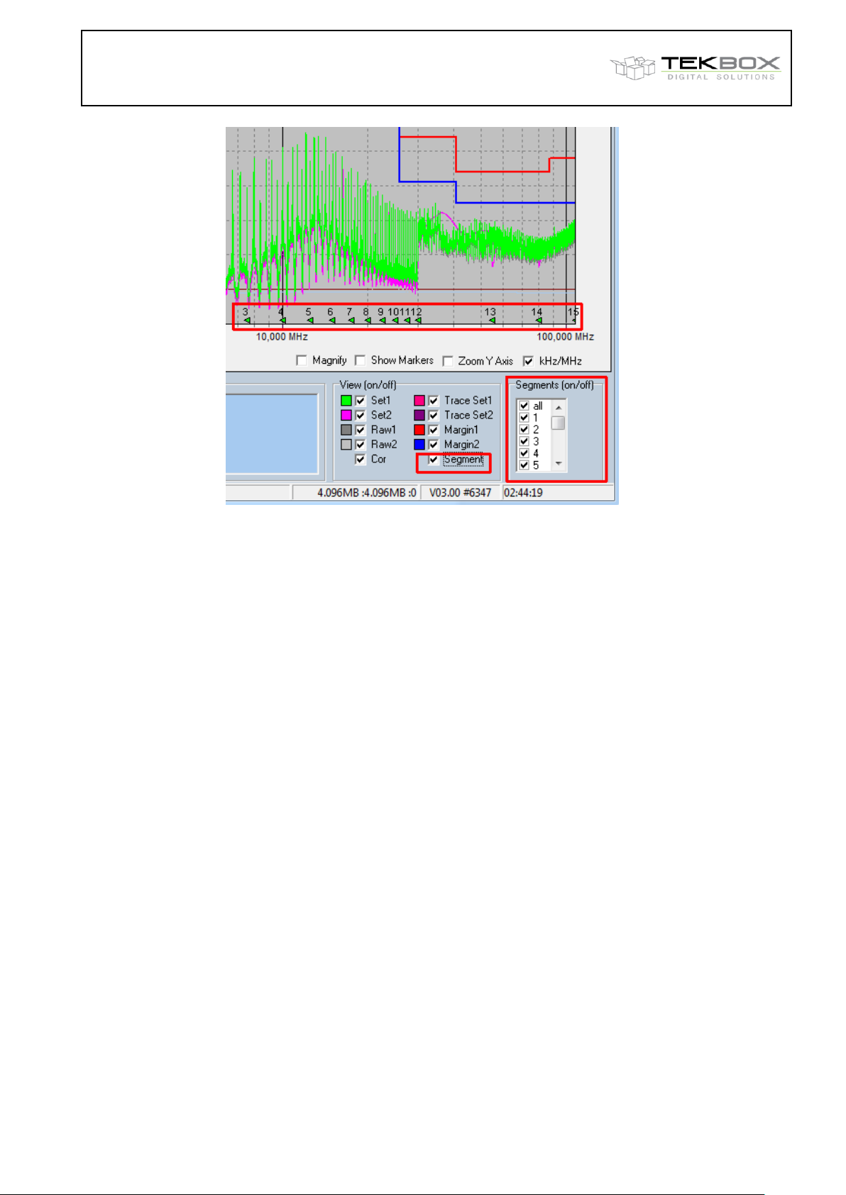
If you want to focus on a certain frequency range when carrying out EMC related improvements of a DUT, you
can shorten time by selectively measure the segments of interest:
Activate displaying the segments by clicking the corresponding box in View (on/off) / Segment. You will then
get the frequency segments displayed at the bottom of the graph. Select the segments that you want to
measure in the Segments (on/off) box. Upon starting a measurement, only the selected segments will be
measured and other segments will be skipped.
By default, skipped segments will be replaced with a straight line. Alternatively, in menu Setup / Options /
Misc, you can select keeping segments from the previous measurement, when skipping it in consecutive
measurements.
Author: Mayerhofer 10 of 29 TekBox Digital Solutions 4-Nov-21
Page 11
Tekbox EMCview Manual_V2_2.docx V2.2
Tekbox EMCview Manual
As Quasi-Peak measurements take much time, an alternative, time saving measurement method is
recommended.
Use a scan with Peak detector and then compare the result against the Quasi-Peak limits. The result of the
Peak detector is always higher or worst case same as the result of a measurement with Quasi Peak detector.
This means, that when passing the Quasi Peak limits with a Peak detector measurement, the DUT is definitely
compliant with Quasi-Peak limits. If the result of the Peak measurement exceeds Quasi Peak limits, there is
still the chance that a measurement with Quasi Peak detector would be within the Quasi Peak limits.
Consequently, a selective Quasi Peak measurement will be carried out, which only looks at the spurious
frequencies where the Quasi Peak limit is exceeded.
The Peak Scan chapter further down describes how such a measurement is carried out.
Pressing the Pause button interrupts ongoing measurements. The current segment will however be
completed, before the measurement pauses. To continue the measurement, press the Play button.
12. SRC folder – compensation files
Any measurement setup has a frequency response which needs to be compensated. The measurement
data delivered by the spectrum analyzer is considered “raw-data”. In order to display Raw Data, activate the
RAW1, RAW2 check boxes in the View (on/off) menu at the right bottom of the EMCview window.
In order to convert the Raw Data into a valid response, compensation files have to be applied. This could be
the LISN file or the trans-impedance file of a current probe in case of conducted noise measurements. In
case of a radiated noise measurement, an antenna factor file would describe the antenna properties and
provide the dBµV to dBµV/m conversion. The measurement set up may also contain cable losses, amplifiers
or attenuators that need to be taken into calculation. The combined frequency response can be displayed by
activating the Cor box in the View (on/off) menu at the right bottom of the EMCview window.
Open existing files from within the COMPENSATION sub directory of the SRC folder to see how to create it.
A compensation file is composed of frequency points with the corresponding value (gain, attenuation,
antenna factor, trans-impedance, etc.)
The frequency range of the compensation file should always cover at least the span of the segment file of
the corresponding project.
Consider the calculation below, if you are not sure about which sign needs to be entered for the
compensation values:
Author: Mayerhofer 11 of 29 TekBox Digital Solutions 4-Nov-21
Page 12
Tekbox EMCview Manual_V2_2.docx V2.2
Margin line for Limit 1, set to 7dB
Tekbox EMCview Manual
Graph amplitude = Raw amplitude [dBµV] – cable file [dB] – LISN file [dB] + ant file [dB] – amp file [dB]
Raw amplitude: spectrum analyzer measurement values
For more information, such as how to deal with current monitoring probe trans-impedance, antenna factors,
unit conversion and other operations that can be carried out using the correction files, have a look at our
EMCview application notes.
Compensation files for Tekbox products can be downloaded on the corresponding product pages of the
Tekbox website.
13. SRC folder – project files
Project files contain a summary of settings for a dedicated measurement set up. In contrary to limit files,
segment files and compensation files, which are created with an editor, project files are usually created from
within EMCview, by setting the graph boundaries, loading the desired limit files and segment files and then
saving it as a project using menu File / Save Proj.
Nevertheless, a user familiar with EMCview, may also use a text editor to create project files.
EMCview contains a large number of pre-defined projects. The projects are loaded using menu File / Load
Proj. Most conducted noise projects reference to Tekbox LISN or current probes. They can easily be
changed, if you have measurement equipment from other manufacturers. Other projects may not yet contain
any compensation files and need to be completed with suitable files for the equipment of your measurement
set up.
Tekbox will regularly provide updates with additional projects. They are part of the installation package, but
they can also be downloaded separately from our web site and manually copied into the SRC folder.
Tekbox also provides compensation files for Tekbox products, which you can find on the corresponding
product pages of www.tekbox.com.
14. Peak scan
Any measurement value of the Set1 run that violates the limit line is indicated with a small bubble on top of
the peak. Activating the MaxFilter box at the bottom of the graph will only mark the highest peaks, if several
consecutive measurement values violate the limit lines.
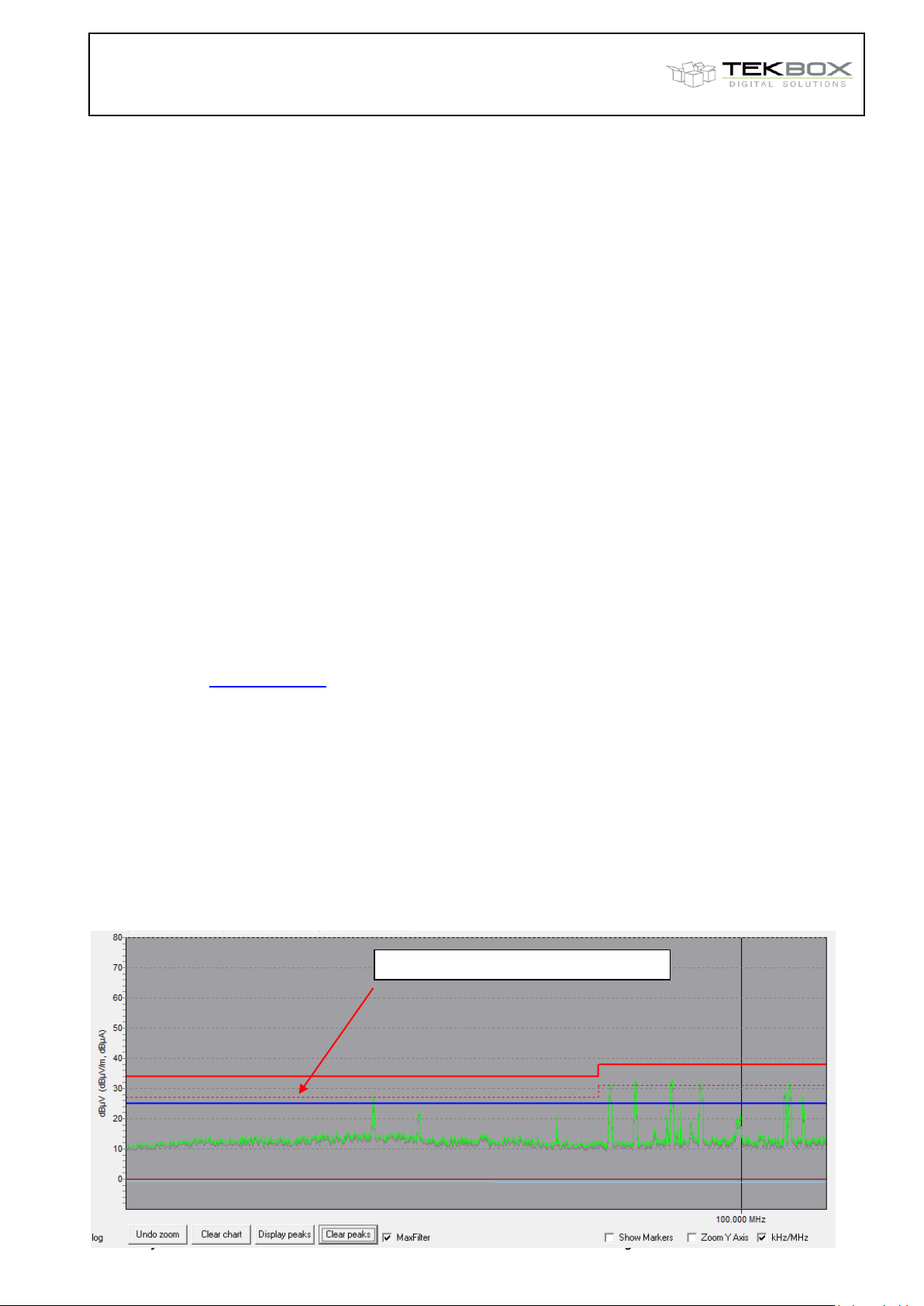
You can define Margins with respect to the limit lines of each measurement set. The SW would then
indicate peaks, which cross the margin lines.
Enter the margin with positive sign to create a dashed line offset below the limit line. Margins with negative
sign can be created as well.
Author: Mayerhofer 12 of 29 TekBox Digital Solutions 4-Nov-21
Page 13
Tekbox EMCview Manual_V2_2.docx V2.2
Tekbox EMCview Manual
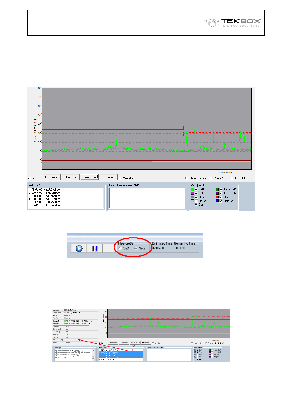
By default, the margins are set to 0, so any peak crossing the limit line would be indicated. Setting margin1
to e.g. 7dB would select all peaks coming within 7 dB close to the limit line of the graph measured with
Settings1. Peaks crossing the margin line or limit line can be listed in the in the Peaks window by pressing
the Display peaks button. See chapter 19 on how to manually select peaks and transfer it into the peaks
list.
In order to display peaks for the second graph, change MeasureSet to set 2
15. Final scan / peak re-measurement
Select any peaks from the list by pressing the Ctrl button and select it with the left mouse button. Then click
the right mouse button and click Measure. There are two measurement options. The recommended choice
is Measure (consider drift).
The software will then re-measure, using the selected peaks as center frequency and using the detector,
sweep time, RBW, Span and PreAmp settings defined in the control box. This feature is a short cut to make
Author: Mayerhofer 13 of 29 TekBox Digital Solutions 4-Nov-21
Page 14
Tekbox EMCview Manual_V2_2.docx V2.2
Tekbox EMCview Manual
a fast Quasi Peak measurement for selected peaks, instead of making a time consuming full span QP
measurement.
Note that with EMCview V 8.0, the settings for peak re-measurement were reduced to the drift span in order
to simplify the user interface and avoid settings which may result in incorrect measurements. All other
settings will be derived from the segment file settings. Refer to the EMCview FAQ document for more
detailed information on fast QP measurements.
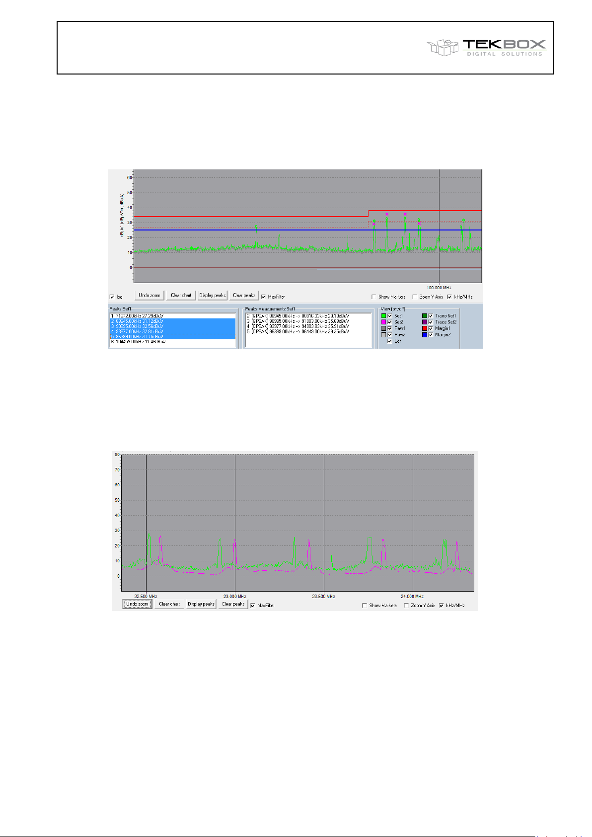
The Peaks Measurements box then displays the results of the fast quasi peak measurement.
In addition, the graph shows a cross at the respective frequency and level.
Consider the span setting of the peak re-measurement, with respect to a potential drift of the peaks. The
higher the drift over time (e.g. drift of the frequency of a switched mode regulator), the wider make the span.
The software will scan the measurement values of the entire span for the highest peak. Consequently, the
frequency of the re-measured peak may deviate from the initial peak frequency. The capability of setting a
Span for a peak re-measurement is an essential feature of EMCview, often missed by similar tools.
The example above illustrates the purpose of the span setting. Harmonics of a switched mode regulator,
which drifted over the time that passed between carrying out the peak measurement (green graph) and the
quasi peak measurement (purple graph). If measured at exactly the peak frequencies of the green graph
using the option Measure (ignore drift), it would completely miss the signals when re-measuring with quasi
peak detector. However, by setting a span of 200 kHz, the quasi peak signal is measured correctly. Use the
option Measure (ignore drift) only if the spurious are harmonics of a crystal clock.
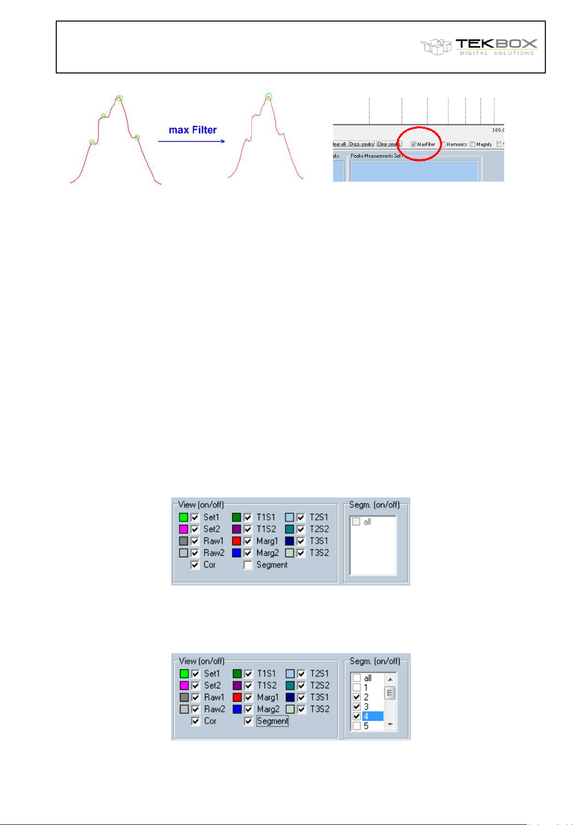
In the measurement graph, peak markers, which are very close to each other may appear to be at the same
frequency, unless zoomed in. Zoomed in, it would look similar as below:
Author: Mayerhofer 14 of 29 TekBox Digital Solutions 4-Nov-21
Page 15
Tekbox EMCview Manual_V2_2.docx V2.2
Tekbox EMCview Manual
Activate the Max Filter box to get rid of these artefacts.
16. View / hide graphs
The graph window can display several traces:
Set 1 corrected graph of the measurement defined by Seg-Set1 and Limit1
Set 2 corrected graph of the measurement defined by Seg-Set1 and Limit1
Raw 1 raw data of Set1 – no LISN, cable, etc. correction
Raw 2 raw data of Set2 – no LISN, cable, etc. correction
Cor correction data of LISN, cable, etc.
Trace1 Set1 imported data from a previous measurement to overlay for comparison purpose
Trace1 Set2 imported data from a previous measurement to overlay for comparison purpose
Trace2 Set1 imported data from a previous measurement to overlay for comparison purpose
Trace2 Set2 imported data from a previous measurement to overlay for comparison purpose
Trace3 Set1 imported data from a previous measurement to overlay for comparison purpose
Trace3 Set2 imported data from a previous measurement to overlay for comparison purpose
Margin1 margin with respect to Limit1
Margin2 margin with respect to Limit2
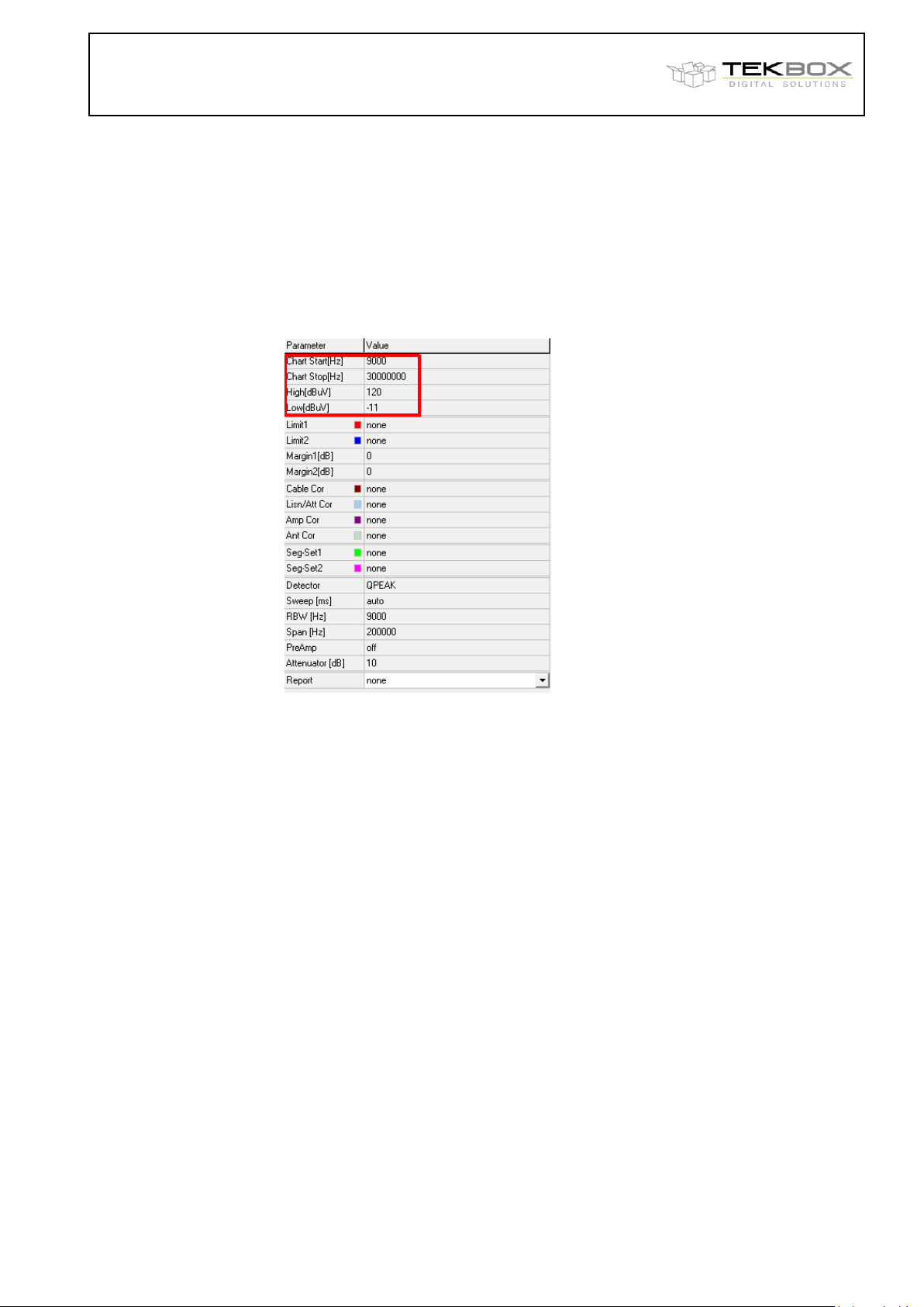
Segment displays the frequency segments, which are defined in the segment file
click Segment to enable measurement of selected segments only
Hide or view traces using the tick boxes in the lower right corner of the window.
Configure colors of traces, limit lines and the background of the graph window in the Setup menu, edit
colors.
Upon selecting the Segment box, the segments defined in the segment file of the current project are
displayed on the frequency axis. Select the segments that you want to re-measure in the segment box in the
lower right corner of the EMCview window.
Author: Mayerhofer 15 of 29 TekBox Digital Solutions 4-Nov-21
Page 16
Tekbox EMCview Manual_V2_2.docx V2.2
Tekbox EMCview Manual
17. Zoom graphs
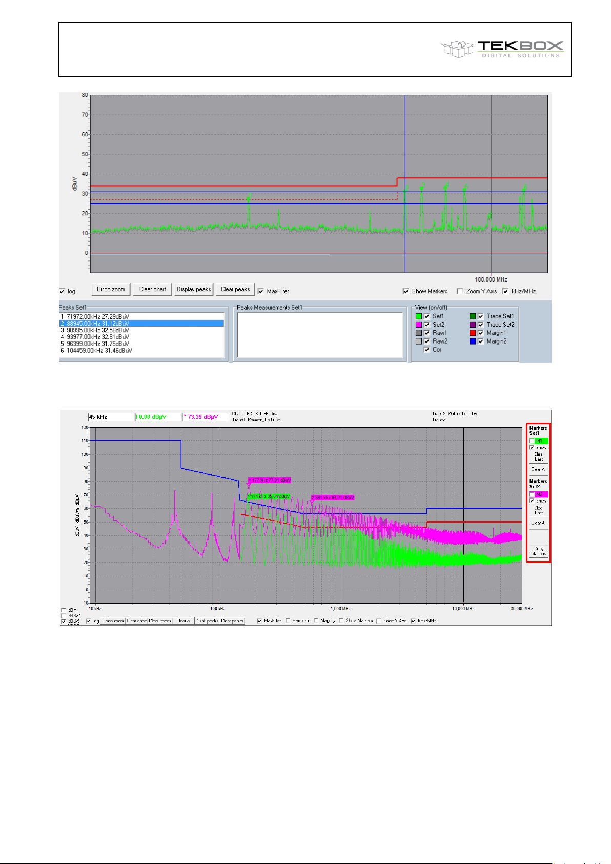
You can zoom or set the boundaries of the graph by entering frequency and amplitude values into the boxes
Chart Start[Hz], Chart Stop[Hz], High[dBµV], Low[dBµV]. Press the TAB button or click another box to
confirm the entered values. During an ongoing measurement, access to the control box is disabled.
Alternatively, you can use the mouse and pull a rectangle in the graph section. When zooming with the
mouse, you can Undo Zoom with a button under the graph window. You can also switch between linear
and logarithmic frequency axis. When zooming in very deeply, the display may be changed automatically to
linear frequency display in order to get a useful grid. Switching to logarithmic frequency axis is not possible
then, unless you Undo Zoom.
To restrict zooming to the y-axis, click the Y-axis check box.
In order to use the magnifying glass to check the graph, click Magnify.
18. Amplitude units
By default, the spectrum analyzer results are taken in dBµV. Antenna or current probe measurements need
conversion files, taking into account antenna factors or trans-impedance to get the y-axis values displayed in
dBµV/m or dBµA. See the corresponding application notes on the EMCview page for more details. Other
than that, units can be selected by ticking the check-boxes next to the lower left corner of the graph window.
19. Markers
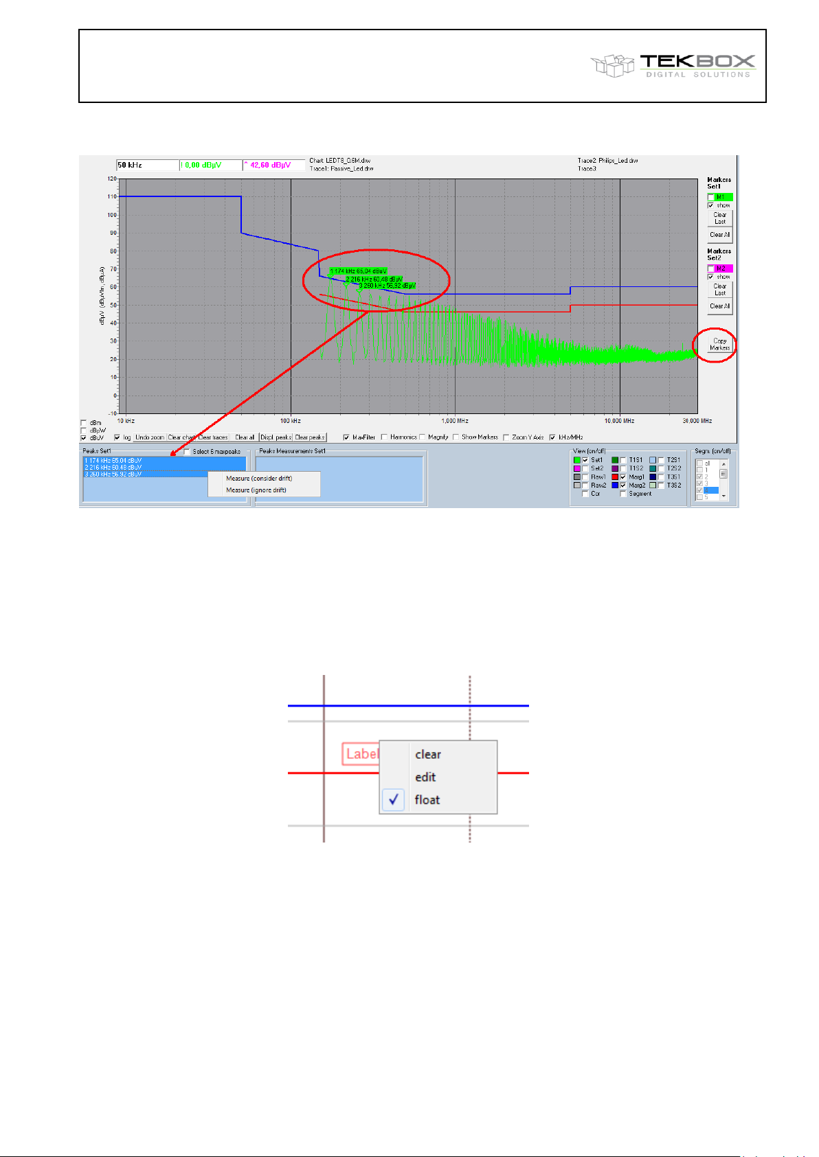
Clicking Show Markers adds the corresponding peak number of the peak list to the graph.
Double clicking any marker in the list will place a cross hair.
Author: Mayerhofer 16 of 29 TekBox Digital Solutions 4-Nov-21
Page 17
Tekbox EMCview Manual_V2_2.docx V2.2
Tekbox EMCview Manual
You can also set markers manually:
Click Marker on the upper right side of the EMCview window.
Click the M1 check box. Thereafter, click at a point of the corresponding graph (Set1) to set a marker.
Click the M2 checkbox, if you want to set a marker to the graph measured according the configuration
specified for Set2.
Author: Mayerhofer 17 of 29 TekBox Digital Solutions 4-Nov-21
Page 18
Tekbox EMCview Manual_V2_2.docx V2.2
Tekbox EMCview Manual
If required, manually set markers can be copied into the Peak list for subsequent re-measurement.
20. Labels
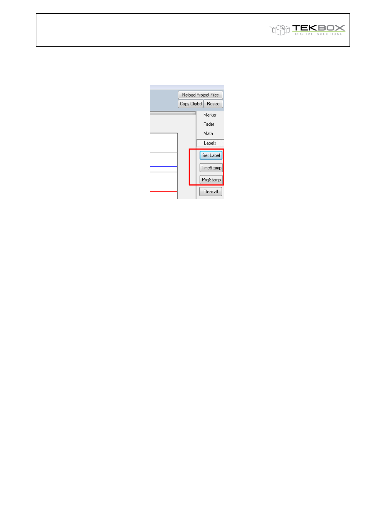
If you want to add comments to the graph, click the Labels button at the right side of the graph.
Click Set Label and a text field will appear in the left upper corner of the graph window. Drag the text field to
the desired position within the graph. Right click into the text field and a context menu will appear:
Click edit to edit the text. De-activate float, if you want to lock the label on its position. The label cannot be
dragged anymore thereafter.
By default, the text field has a frame. If you want to remove the frame, enter menu Setup / Options and set
it to transparent.
If you want to change the font size of the labels, edit the emcview.ini file that you can find in the installation
folder of EMCview. Change the TextSize1 parameter to the desired value.
The color of the labels can be changed in the Setup / Edit Colors menu of EMCview. Note that you can
only change the color of all labels, but not change colors of individual labels.
Author: Mayerhofer 18 of 29 TekBox Digital Solutions 4-Nov-21
Page 19
Tekbox EMCview Manual_V2_2.docx V2.2
Tekbox EMCview Manual
Within Labels, you can also set a Time Stamp Label and a Project Stamp label. Any time, the TimeStamp
button is clicked, it will update date and time. In Setup / Options menu, you can set the time stamp label
being updated, any time you press the Copy Clipbd button.
21. Options
In menu Setup / Options you can set various preferences:
Path / Out: by default, all files are saved in the EMCview\Out directory. Here you can change your
preferred default output directory.
Misc / Enable dialog box to conform closing EMCview: Close EMCview immediately or upon confirming
in a dialog box
Misc / Load last project: Launch EMCview with the project file used when last exiting EMCview
Misc / Show TG box to enable TG during RF measurement sweep: In preparation of a future feature to
create amplitude correction files using the tracking generator of the analyzer
Misc / Enable sweep step size in %: Add a selection box in the generator feature to select sweep step size
either in Hz or in %
Misc / Report marked peaks only: In order to avoid an excessively long peak list in the report file, the
listed peaks can be limited to selected (marked) peaks from the peaks list
Misc / Show full names of loaded charts and traces: When loading charts or traces, they will be
displayed on top of the graph window. If the file names are excessively long and exceed the available
display space, they will be cropped to a suitable length.
Misc / Keep old segments, when re-measuring selected segments: When making selective
measurements, keep results of previous measurements for skipped segments instead of connecting it with a
straight line.
Misc / Show checkbox for consecutive measurement of both sets: This adds a checkbox next to the
measurement button to choose to automatically run Set2 after Set1 has finished.
Misc / Monitor SCPI communication link: Indicates in the status line, if the communication link between
PC and analyzer is interrupted (green hook/red x).
Misc / Show VISA errors: Displays Visa error messages in a pop up window
Labels / Draw labels transparent: Removes frame and background of the label text boxes
Labels / Update time stamp when copying to clipboard: Updates the time stamp label, when the graph
window is copied to the clip board
Author: Mayerhofer 19 of 29 TekBox Digital Solutions 4-Nov-21
Page 20
Tekbox EMCview Manual_V2_2.docx V2.2
Tekbox EMCview Manual
22. Fader
The “fader” is a feature to cancel ambient noise when measurements are carried out in a non-shielded
setup. It needs to be mentioned upfront, that it is no alternative to measurements in shielded chambers or
tents. Main reason for implementing the fader feature was repeated customer request.
The fader is based on making a measurement of the ambient noise, with the DUT not powered and then
subtracting the ambient noise from a consecutive measurement, with the DUT powered.
However, ambient noise is hardly ever static. Cellular radio signals are highly dynamic both in frequency and
amplitude. Broadcast stations create ambient noise with static frequency, however they drift in amplitude.
Subtracting such signals will not cancel completely or may result in negative spikes, if their amplitude does
not remain constant, but decrease or increase in the time between taking the un-powered measurement and
the powered measurement.
Consequently the fader does not take the entire ambient noise spectrum, but gives the user the capability to
select portions of the noise spectrum that he wants to subtract.
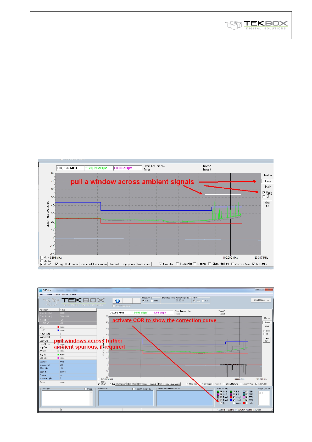
To use the fader, first take a measurement with the DUT not being powered. Then click the Fader button at
the right side of the graph window and activate the fade box. Then left click the mouse to pull a window
across the noise that you want to get subtracted when you do a powered measurement.
Activate the Cor box to see the resulting correction curve.
Author: Mayerhofer 20 of 29 TekBox Digital Solutions 4-Nov-21
Page 21
Tekbox EMCview Manual_V2_2.docx V2.2
Tekbox EMCview Manual
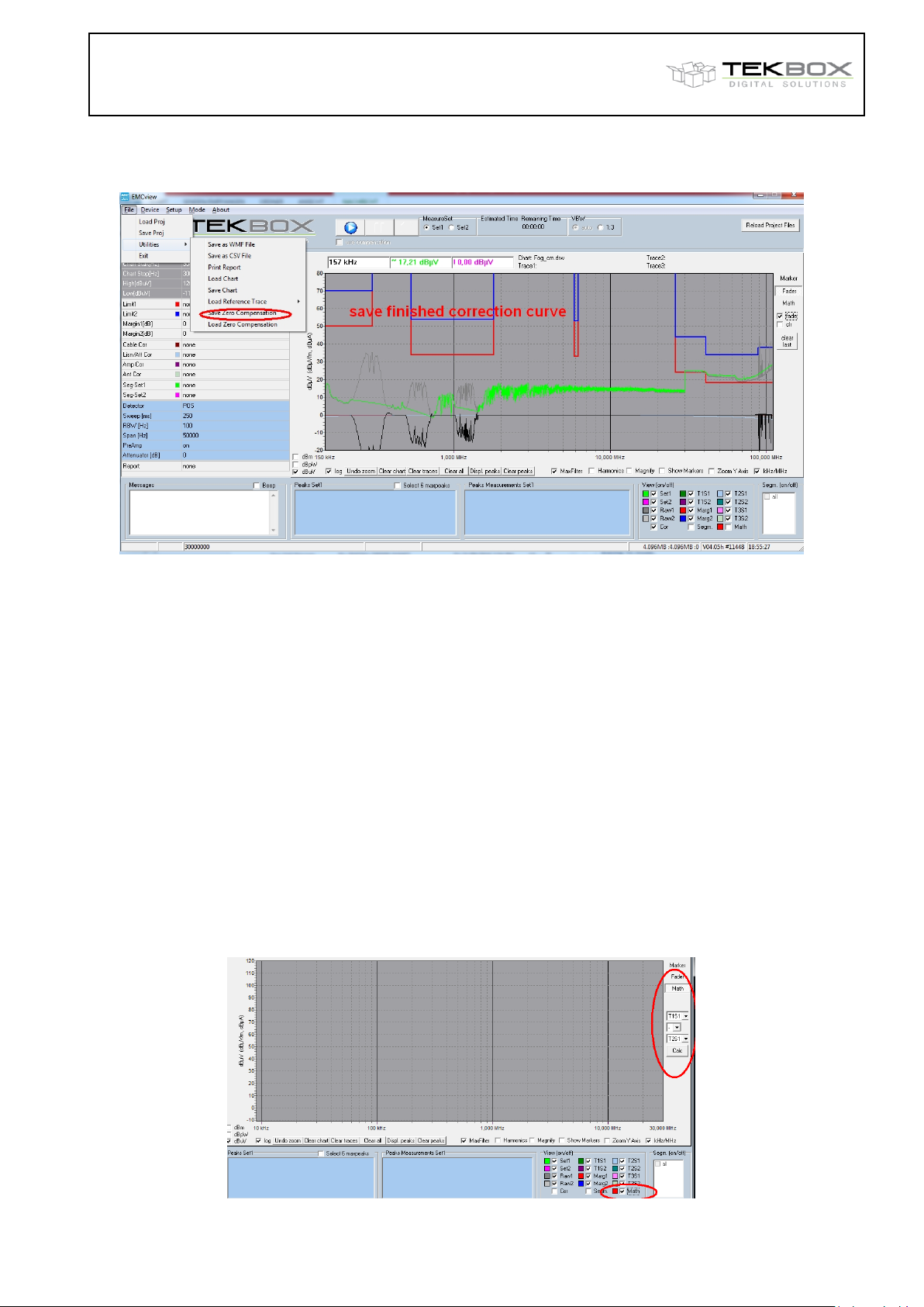
Repeat this process for other noise spurious, if required.
Next save the correction curve in File, Utilities, Save Zero Compensation.
In order to apply the correction curve to the powered measurement, load the correction curve in File,
Utilities, Load Zero Compensation. Then click the box use compensation (fader compensation) located
under the Play button.
Then start another measurement run, with the DUT being powered. The correction curve will then
immediately be applied to this measurement.
As mentioned – don´t expect miracles from this feature. A perfect cancellation will only be achieved for
ambient noise signals that remained perfectly constant with respect to frequency and amplitude. Also be
aware, that any DUT noise hidden under the ambient noise will not be recovered.
23. Math
“Math” is a feature to add, subtract, multiply or divide traces. The traces need to be loaded into EMCview
before being able to carry out mathematical operations.
Click the Math button located right to the graph window. Then select the traces, select the mathematical
operation and click the Calc button to get the result displayed in the graph window. In order to view the
resulting graph, activate the Math button in the View (on/off) window.
If you take for example conducted noise measurements of the positive and negative supply line and want to
merge it to a worst case graph, load the traces and use the MAX operation.
Author: Mayerhofer 21 of 29 TekBox Digital Solutions 4-Nov-21
Page 22
Tekbox EMCview Manual_V2_2.docx V2.2
Tekbox EMCview Manual
24. Saving graphs and measurement results
Save data in File menu, Utilities, Save Chart. The chart (graph) of any measurement can be reloaded into
EMCview clicking Load Chart. Clicking Load Chart overwrites any graph present on the screen.
Reload and overlay older measurements to a fresh measurement for comparison purpose by clicking Load
Reference Trace in the same menu. This feature adds (overlays) one or two more graphs to the existing
measurement or chart. Restarting a measurement will clear the graph of the previous measurement, but not
affect the Reference Trace.
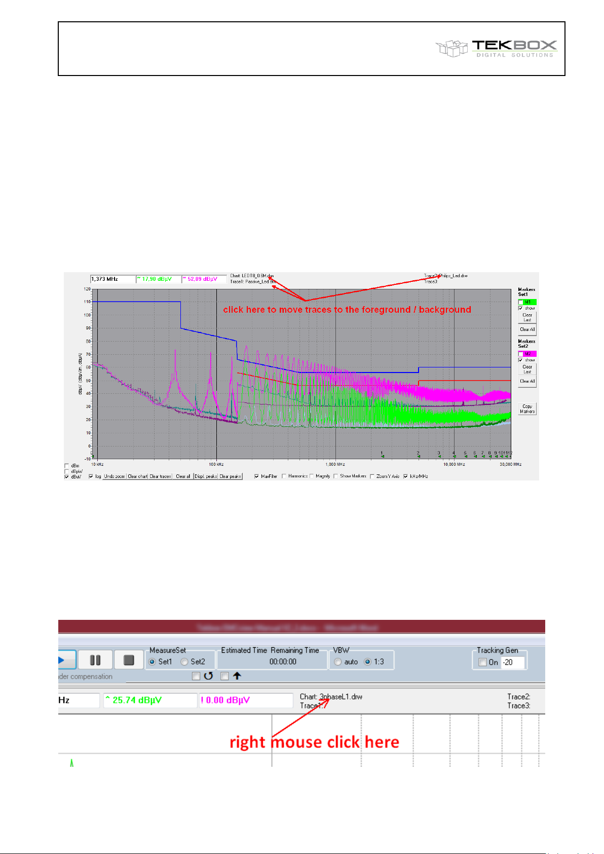
In order to bring any of the reference traces to the foreground, click at the line listing the trace file. Click at
the text again to bring it to the background.
Click Save as WMF File to save chart screen shots.
Click Save as CSV File to save the measurement result as table.
You can save peak lists as text file, right clicking in the peak window and selecting Save to File in the
context menu.
Charts are always saved including the amplitude correction data. If you figure out, that you applied wrong
correction files, after completing a measurement, you can save the chart and then reload it as raw data and
select different amplitude correction files.
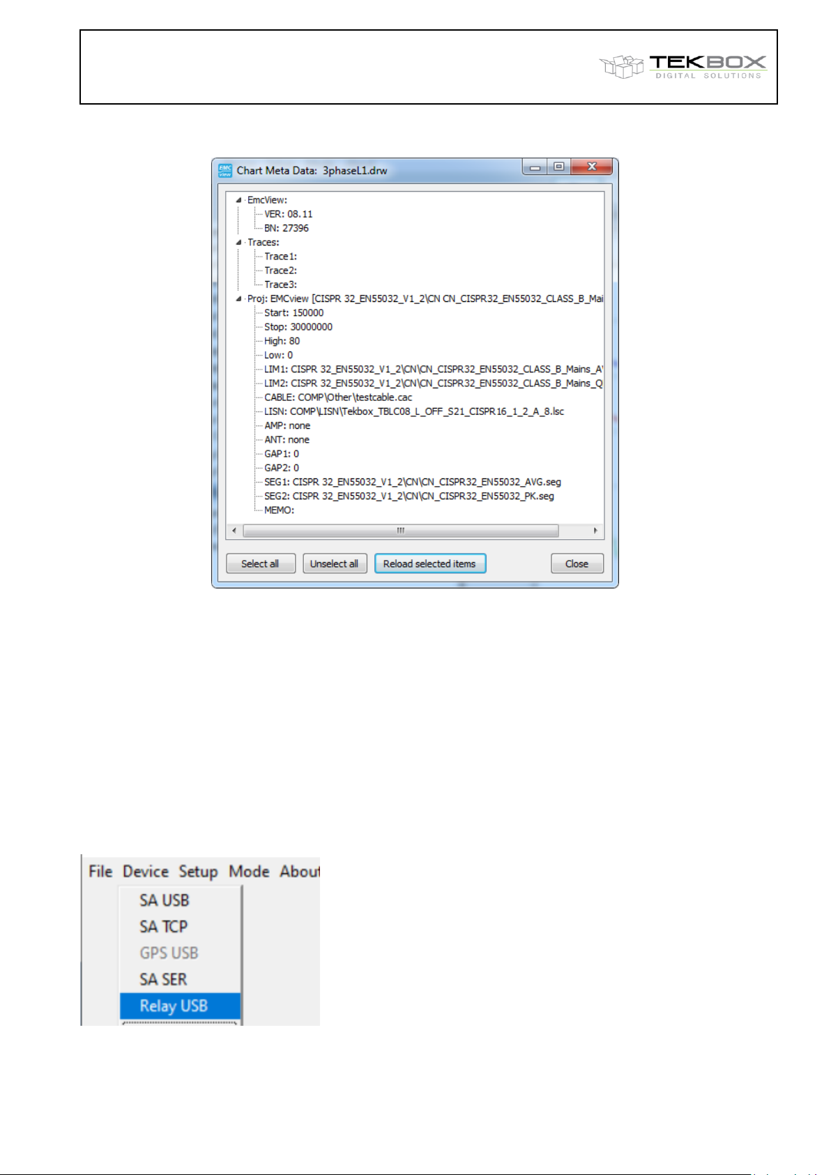
With EMCview V8.12, meta data is added when saving charts. You can restore the entire set up of EMCview
of the point you carried out your measurement and saved the chart. This not only includes the set up, chart
and correction data, but also any trace, which was loaded when saving the chart. Load the chart and then
right click at the chart string displayed on top of the graph window, after loading the chart:
Author: Mayerhofer 22 of 29 TekBox Digital Solutions 4-Nov-21
Page 23
Tekbox EMCview Manual_V2_2.docx V2.2
Tekbox EMCview Manual
After right clicking, following window will pop up:
Click Select all and Reload selected items, if you want to restore the entire set up or make a selection by
clicking any of the lines. Note that restoring only works correctly, if all involved files are still present in its
original location.
25. Control of additional equipment with EMCview
With EMCview V5.48 or higher, commands for ASCII controllable devices can be added to the segment
files. You can use a device such as KMTronic 4UCRB Relay Controller to switch coaxial antenna relays or
external attenuators.
Go to menu DEVICE to connect to the relay controller:
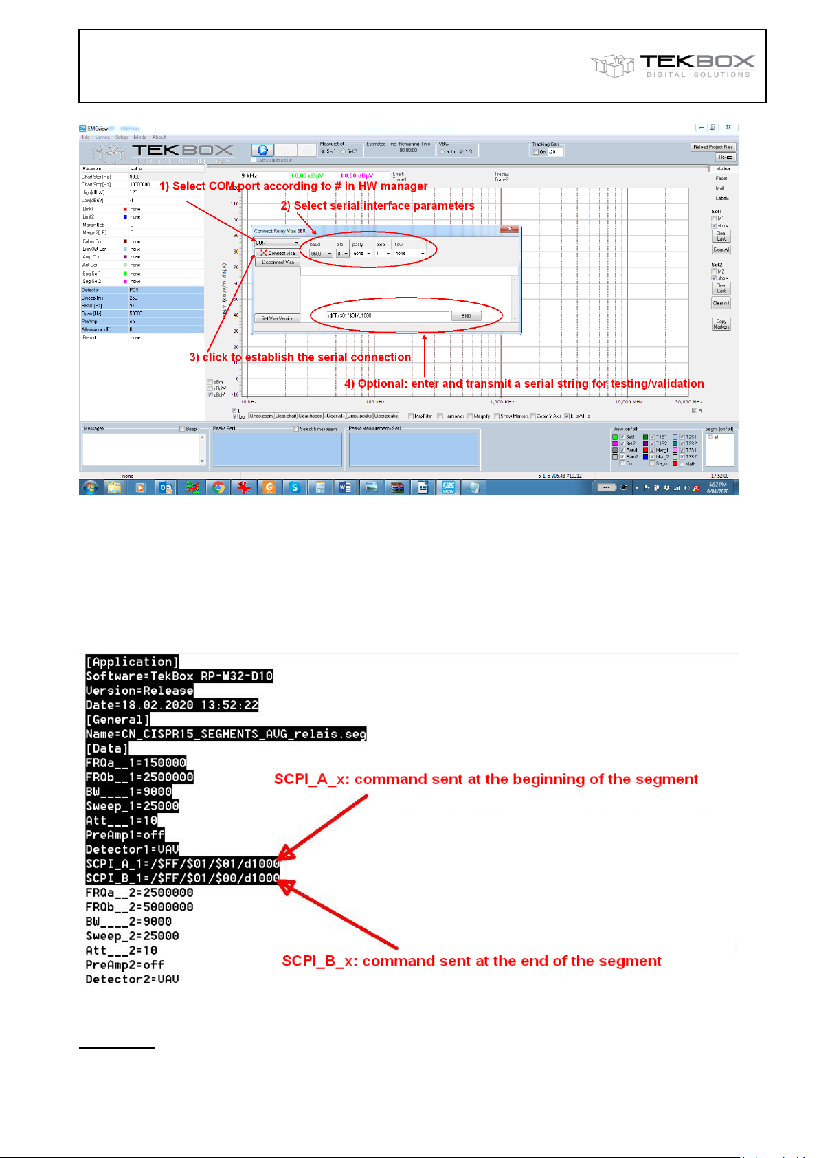
Next select the COM port and set up the parameters for the serial interface of the relay controller or any
other serial device. Establish the connection and optionally transmit a string for testing/validation:
Author: Mayerhofer 23 of 29 TekBox Digital Solutions 4-Nov-21
Page 24
Tekbox EMCview Manual_V2_2.docx V2.2
Tekbox EMCview Manual
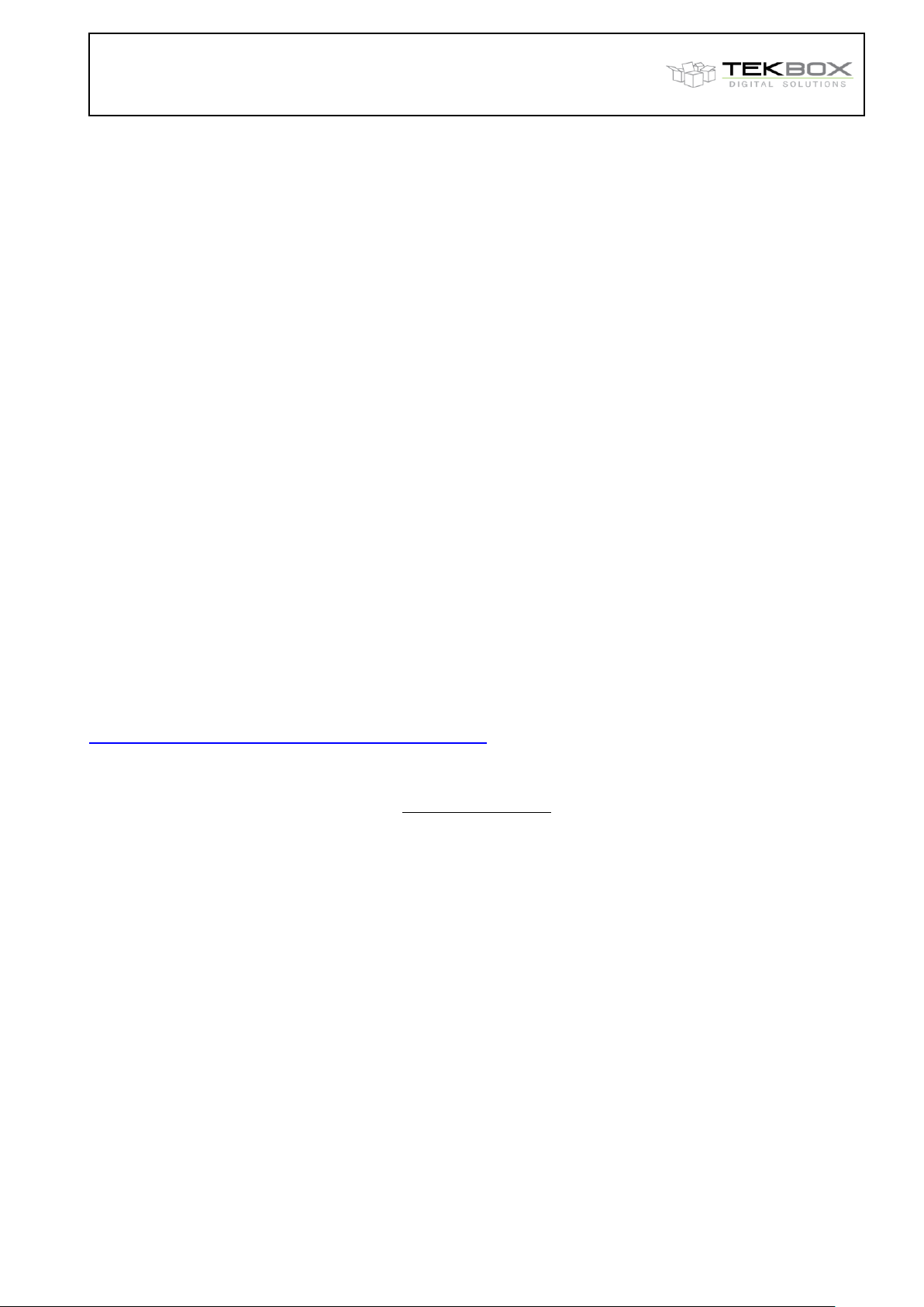
In order to automatically transmit test strings, they need to be entered into the desired segment file.
You can add two serial command strings to each segment. Command SCPI_A will be executed before the
sweep of the corresponding segment. Command SCPI_B will be executed after the sweep of the
corresponding segment.
Example: Segment file with commands for the KMTronic 4UCRB Relay Controller
Explanation:
SCPI_A_x with x being the segment number; command sent at the beginning of the segment
Author: Mayerhofer 24 of 29 TekBox Digital Solutions 4-Nov-21
Page 25
Tekbox EMCview Manual_V2_2.docx V2.2
Tekbox EMCview Manual
SCPI_B_x with x being the segment number; command sent at the end of the segment
SCPI_B_x is optional. A single command at the beginning of the segments would be sufficient to turn
ON/OFF a relay.
/$FF/$01/$01: serial string to turn on output 1 of the KMTronic 4UCRB Relay Controller. It will send the
characters FF 01 01. This string is not EMCview specific. Its syntax has to be chosen according to the
manual of the corresponding device. FF 01 01 means turn ON Output 1 of the 4UCRB. EMCview will send
whatever string is entered in this place.
/d1000: wait 1000 ms before starting the sweep. Maximum value: 9999 ms
Special control commands can be entered as /$XX (upper case, always 2 characters)
Example:
/$0A LF, Line Feed (not /$0a)
/$0D CR, Carriage Return (not /$cr)
26. Using RF current probe measurements to extrapolate to
radiated E-field strength
Signal- and power supply cables carrying conducted noise act as antennas and consequently cause
radiated emissions.
Henry Ott and Clayton Paul outlined a method to convert RF current probe measurements into electric field
strength radiated from cables carrying RF currents. It is a derivation/simplification of the full treatment outlined
in “Antenna Theory – Analysis and Design” (C. Balanis).
This application note is based on an excellent article on the website of Andy Eadie from EMC FASTPASS.
The application note explains how this method can be applied, using Tekbox EMCview software. It
automatically creates a graph of radiated emissions, converting a common mode current conducted noise
measurement carried out with a RF current probe and a spectrum analyzer.
Andy Eadie´s article can be found here:
https://emcfastpass.com/current-probe-e-field-emi-testing/
“The Formula”
𝐸 =
E = electric field strength [V/m]
f = frequency [Hz]
I = CM current [A]
L = cable length [m]
r = measurement distance [m]
Ɵ = π/2
According to Andy Eadie’s article, this formula delivers a very accurate result up until approximately 200
MHz with a 1m cable.
The Tekbox application note AN_ RF current to electric field strength extrapolation shows two methods how
to calculate and display the E-field using EMCview. Refer to this document for detailed instructions.
4𝜋 ∙ 10
−7
(
𝑓 ∙ 𝐼 ∙ 𝐿)𝑠𝑖𝑛𝜃
𝑟
27. Create Reports
Click Setup, Edit Report. Click Clear and then enter the report details. Click Save and enter a file name.
In order to print the report, click File, Utilities, Print Report. If you want to keep the report as a file, print using
a pdf writer. To do so, set a pdf writer as default printer in Windows settings.
Author: Mayerhofer 25 of 29 TekBox Digital Solutions 4-Nov-21
Page 26
Tekbox EMCview Manual_V2_2.docx V2.2
Tekbox EMCview Manual
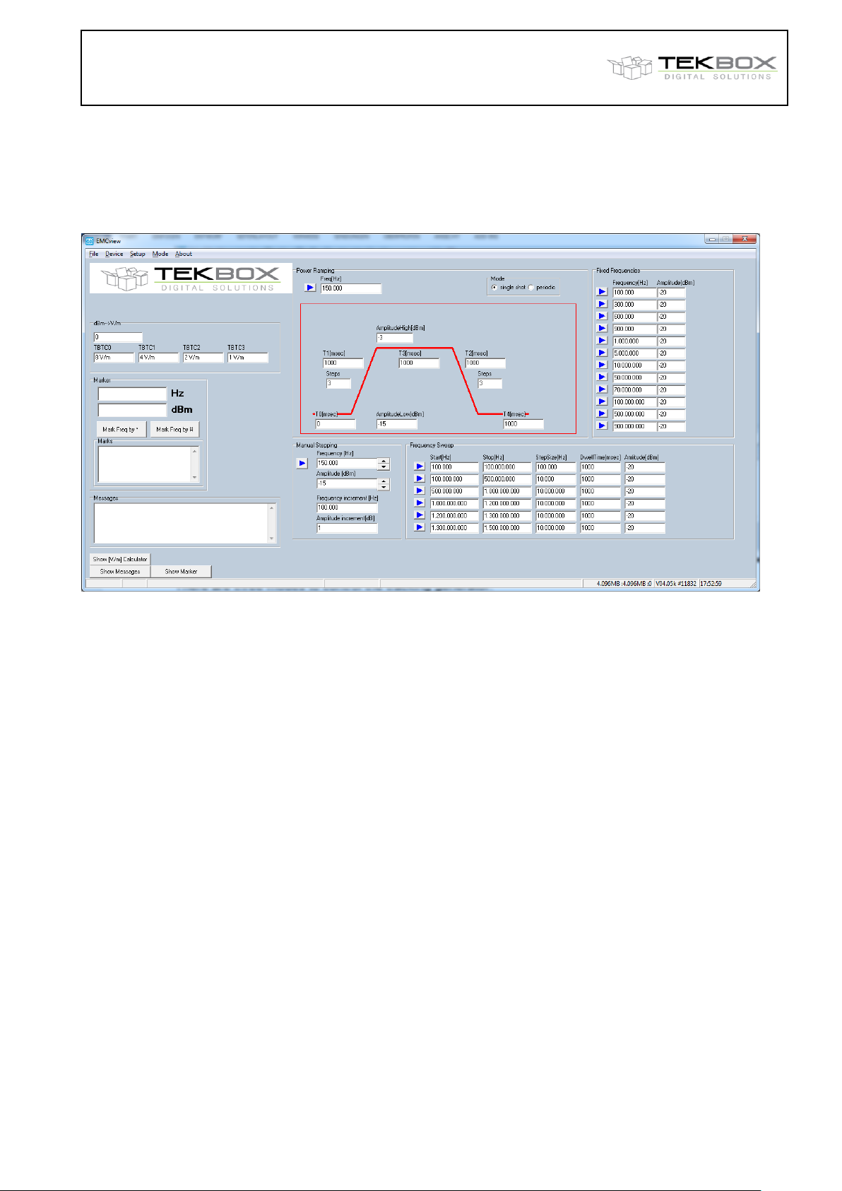
28. Tracking generator control mode for immunity testing
A spectrum analyzer equipped with tracking generator, together with a TEM Cell and a modulated power
amplifier from Tekbox can be used very effectively for pre-compliance immunity testing.
In order to simplify tracking generator control, click menu Mode / Generator.
There are three modes to control the tracking generator:
Power Ramping generates a configurable power ramp profile at a fixed frequency; either as a single
pulse or periodic.
Frequency Sweep carries out a frequency sweep with configurable start and stop frequency, frequency
step size, output level and dwell time per frequency point.
Fixed Frequencies sets the generator to a fixed output frequency and output level
Manual Stepping manually step frequency and amplitude of the tracking generator
Consider that the amplitude of most tracking generators are limited to the range -20dBm to 0 dBm and to an
amplitude step size of 1 dB. For lower output levels, use an external attenuator; for higher output levels use
an external amplifier.
An immunity pre-compliance test will typically start with a frequency sweep. The DUT is placed inside a TEM
cell and a wideband amplifier will boost the TG signal to the necessary level to create a strong electric field
inside the TEM cell. Observe the DUT for any misbehavior during the sweep. In case of observing any DUT
malfunction, press the Mark Frequency tab to record the frequency.
In order to save time during later re-testing, after modification of the DUT, change to fixed frequency mode,
using critical frequencies observed during the sweep.
Check our website for corresponding application notes and for the EMCview FAQ document from time to time.
29. RF coverage measurement mode
In RF coverage measurement mode, the field strength of up to 3 transmitters can be monitored in parallel.
GPS coordinates are assigned to every measurement sample. EMCview currently supports Opus / Eride
chipset based GPS receivers with NMEA output via USB. A suitable GPS receiver is also available from
Tekbox.
Author: Mayerhofer 26 of 29 TekBox Digital Solutions 4-Nov-21
Page 27
Tekbox EMCview Manual_V2_2.docx V2.2
Tekbox EMCview Manual
In order to make RF coverage measurements, connect to the spectrum analyzer and GPS receiver in the
Device menu. Click Mode, RF Coverage to enter RF coverage measurement mode.
29.1 Configuration
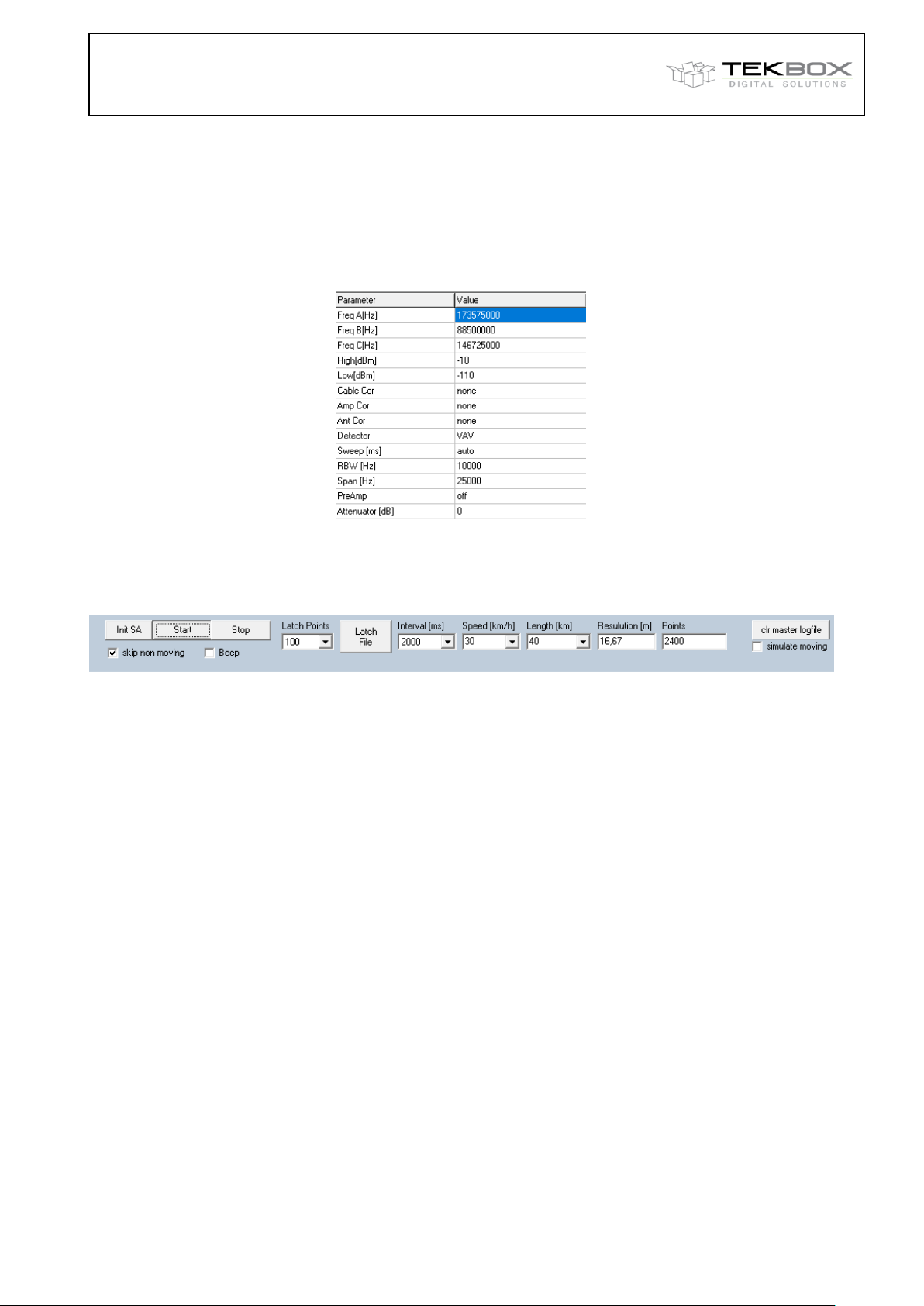
Enter the frequencies that you want to observe along with the spectrum analyzer settings:
If Freq(B) and or Freq(C) are not required for the measurement, simply delete the contents of the
corresponding box.
High[dBm], Low[dBm] values specify the y-axis display range of the graph. The values on the X-axis
correspond to the index of the consecutive measurement samples.
Init SA: transfers the measurement settings to the spectrum analyzer and initialize the SW for
a new measurement
Start: start measurement or continue interrupted measurement; requires a GPS fix and
established connection to the spectrum analyzer.
Stop: stop measurement
Latch Points: select the number of measurement points, after which a KML file will be created
automatically. If the total number of measurement points exceeds the settings in
Latch Points, additional KML files will be created.
Latch File: creates a KML file upon pressing the button
Interval [ms]: time in between two consecutive measurements (measurement interval). Minimum
time largely depends on number of observed frequencies, sweep time and
measurement response time of the analyzer. With the analyzer settings in the
example above, 3 frequencies can be monitored every 2 seconds. If the set interval
time is too low, a timing error will be occur and increment the T3-Err counter at the
bottom of the graph.
Speed [km/h]: enter the estimated average speed of your measurement drive here to calculate the
resolution of your measurement
Length [km]: enter the estimated length of your measurement drive here to calculate the resulting
number of measurement points
Resolution[m]: average distance between two measurement points based on the entered value of
Speed and the settings for the measurement interval.
Points: resulting number of measurement points based on the estimation of the length of the
measurement drive and the settings for the measurement interval.
Clr master logfile: the data of every measurement point is logged into a text file with file name
coverage.txt. Any additional measurement will be appended to existing data in the
log file. Press this button to delete the contents of the log file. The log file is located in
the sub directory \out.
Skip non moving: Don´t log any measurement points if the speed reported by the GPS receiver is zero
Author: Mayerhofer 27 of 29 TekBox Digital Solutions 4-Nov-21
Page 28
Tekbox EMCview Manual_V2_2.docx V2.2
Tekbox EMCview Manual
Simulate moving: only to validate the measurement setup; don´t click for an actual measurement. The
SW generates a random offset to the coordinates measured by the GPS receiver to
simulate a test drive.
29.2 Status and measurement results
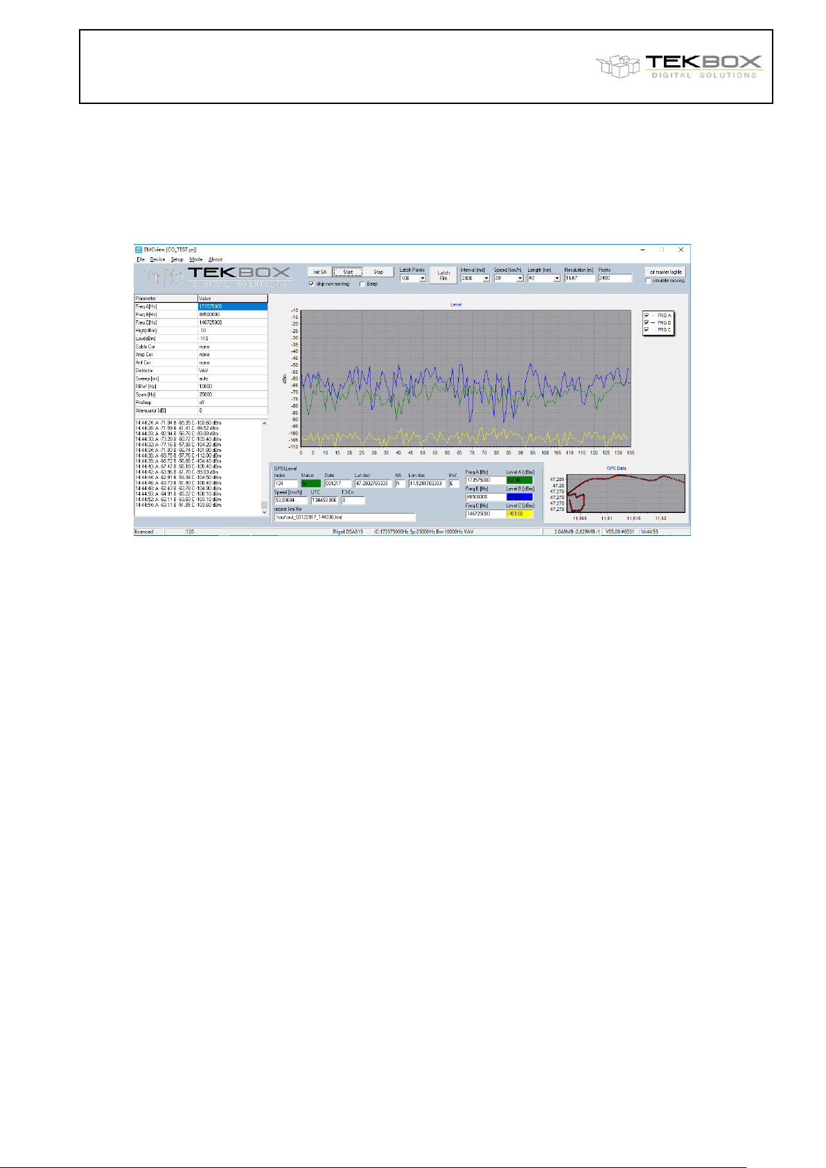
The main graph displays the measured field strength of the observed transmitters on the y- Axis and the index
number of the corresponding measurement on the X-axis.
The GPS data window displays the coordinates of consecutive measurement points.
Index: index counter; number of current measurement sample
Status: displays GPS fix
Date: current date
Lat dec: current latitude in decimal format
NS: latitude north/south
Long dec: current longitude in decimal format
EW: latitude east/west
Speed: current speed
UTC: current time
T3-Err: error counter, counts timer errors caused by insufficient length of measurement interval
Freq A: observed frequency A
Level A: field strength/ amplitude of transmitter A
Freq B: observed frequency B
Level B: field strength/ amplitude of transmitter B
Freq C: observed frequency C
Level C: field strength/ amplitude of transmitter C
Recent kml file: shows the path and file name of the latest generated kml file: default directory is \out. The kml
file is created automatically and consists of the string out_date_time.kml.
29.3 Log file
The index file is a text file containing an index for each sample, date, time, longitude, latitude, speed, observed
frequencies and corresponding field strength.
Example:
Index;Fix;Date;UTC;Lat;NS;Long;EW;Speed[km/h];FreqA[Hz];LevA[dBm];FreqB[Hz];LevB[dBm];FreqC[Hz];LevC[dBm]
0;fix;031217;133951.086;47.2786633333;N;11.5031383333;E;19,8164;173575000;-61.62;88500000;-55.71;146725000;-102.30
1;fix;031217;133953.086;47.2785533333;N;11.5031883333;E;23,46484;173575000;-66.53;88500000;-67.06;146725000;-104.70
2;fix;031217;133955.086;47.2784366667;N;11.5032450000;E;24,20564;173575000;-77.26;88500000;-58.54;146725000;-104.80
3;fix;031217;133957.086;47.2783266667;N;11.5033033333;E;22,35364;173575000;-86.61;88500000;-56.00;146725000;-104.00
….
Author: Mayerhofer 28 of 29 TekBox Digital Solutions 4-Nov-21
Page 29
Tekbox EMCview Manual_V2_2.docx V2.2
Version
Date
Author
Changes
V 1.0
20.04.2017
Mayerhofer
Creation of the document
V 1.1
26.04.2017
Mayerhofer
Chapter 2 (warnings) added
V 1.2
21.06.2017
Mayerhofer
Siglent support added
V 1.3
16.12.2017
Mayerhofer
Updates - SW REV 3.0
V 1.4
6.6.2018
Mayerhofer
Updates - SW REV 4.0
V 1.5
9.10.2018
Mayerhofer
Updates - SW REV 4.05
V 1.6
9.10.2018
Mayerhofer
Chapter 1 and 2 updated
V 1.7
9.4.2020
Mayerhofer
Chapter 1, 2, 16, 18 and 22 updated
V 1.8
6.5.2020
Mayerhofer
Chapter – SW REV 6.01
V 1.9
6.5.2020
Mayerhofer
Chapter 22 inserted – SW REV 6.07
V 2.0
25.9.2020
Mayerhofer
Chapter 9, 10, 12, 13 inserted – SW REV 7.0
V 2.1
1.4.2021
Mayerhofer
Information on changed peak re-measurement
UI with EMCview V8.0
V 2.2
4.11.2021
Mayerhofer
Information on restoring measurement set-ups
with EMCview V8.12 and higher
Tekbox EMCview Manual
29.4 KML file
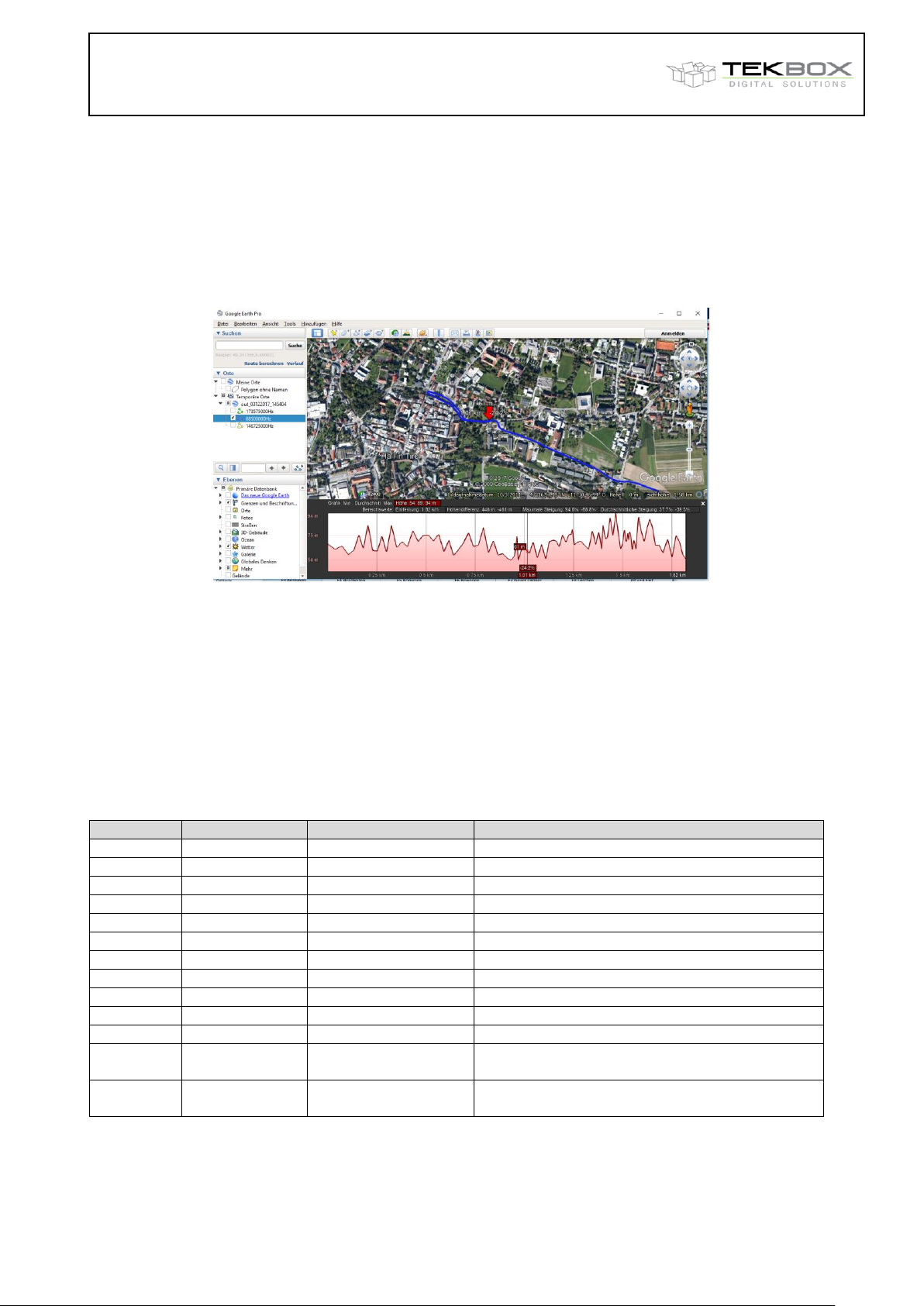
The KML file can be used to project the measurement drive into Google Earth Professional.
The altitude-profile graph feature of Google Earth Professional is utilized to display a field strength profile. The
[m] unit displayed by Google Earth is equivalent to the measured amplitude in [-dBm]. Consequently, peaks
in the graph represent lower field strength values, means the graph is mirrored on the x-axis.
In Google Earth menu View, reset tilt. If you don´t see the track, in Layers, activate More. In order to see the
field strength profile, click the Edit menu and then show elevation profile.
30. Further information
Read the EMCview FAQ document for more detailed information. Also
check our website from time to time for software updates, new project
packages and useful application notes.
31. History
Author: Mayerhofer 29 of 29 TekBox Digital Solutions 4-Nov-21
 Loading...