

Page 1

Syscomp Computer Controlled Instruments
CTR-201 Curve Tracer
Syscomp Electronic Design Limited
http:\\www.syscompdesign.com
Revision: 2.1
November 2017
Page 2

Revision History
Version Date Notes
1.00 November 2014 First revision
1.10 April 2015 Feature Update
1.11 March 2016 Solar cell option added
2.1 November 2017 New software and hardware
Contents
1 Introduction 1
2 The CTR-201 Curve Tracer 2
3 Measurements 4
3.1 Device Connections . . . . . . . . . . . . . . . . . . . . . . . . . . . . . . . . . . . . . . . . . 4
3.2 Instrument Overview . . . . . . . . . . . . . . . . . . . . . . . . . . . . . . . . . . . . . . . . 4
3.3 Diode . . . . . . . . . . . . . . . . . . . . . . . . . . . . . . . . . . . . . . . . . . . . . . . . 7
3.4 Zener Diode . . . . . . . . . . . . . . . . . . . . . . . . . . . . . . . . . . . . . . . . . . . . . 7
3.5 NPN Transistor (BJT) . . . . . . . . . . . . . . . . . . . . . . . . . . . . . . . . . . . . . . . . 9
3.6 PNP Transistor (BJT) . . . . . . . . . . . . . . . . . . . . . . . . . . . . . . . . . . . . . . . . 10
3.7 N-Channel MOSFET . . . . . . . . . . . . . . . . . . . . . . . . . . . . . . . . . . . . . . . . 10
3.8 P-Channel MOSFET . . . . . . . . . . . . . . . . . . . . . . . . . . . . . . . . . . . . . . . . 11
3.9 N-Channel JFET . . . . . . . . . . . . . . . . . . . . . . . . . . . . . . . . . . . . . . . . . . 11
3.10 Gene ral 2-Terminal Measurement . . . . . . . . . . . . . . . . . . . . . . . . . . . . . . . . . 13
3.10.1 2-Terminal Measurement, Voltage Mode . . . . . . . . . . . . . . . . . . . . . . . . . . . 13
3.10.2 2-Terminal Measurement, Curren t Mode . . . . . . . . . . . . . . . . . . . . . . . . . . 14
3.11 Small Signal Transistors . . . . . . . . . . . . . . . . . . . . . . . . . . . . . . . . . . . . . . 14
3.12 Solar Cells . . . . . . . . . . . . . . . . . . . . . . . . . . . . . . . . . . . . . . . . . . . . . . 14
3.13 Lam bda Diode, Negative Resistance Device . . . . . . . . . . . . . . . . . . . . . . . . . . . . 15
3.14 Vacuum Tube . . . . . . . . . . . . . . . . . . . . . . . . . . . . . . . . . . . . . . . . . . . . 15
4 How It Works 16
5 Calibration 21
6 Installing the Software 23
6.1 Packaged Executable . . . . . . . . . . . . . . . . . . . . . . . . . . . . . . . . . . . . . . . . 23
6.2 Source Code . . . . . . . . . . . . . . . . . . . . . . . . . . . . . . . . . . . . . . . . . . . . . 23
6.2.1 Obtaining the Source Code . . . . . . . . . . . . . . . . . . . . . . . . . . . . . . . . . . 23
6.2.2 Installing the Tcl Interpreter on a Windows Machine . . . . . . . . . . . . . . . . . . . . 24
6.2.3 Executing the Sou rce Code . . . . . . . . . . . . . . . . . . . . . . . . . . . . . . . . . . 24
7 Commands 24
7.1 Testing the Commands . . . . . . . . . . . . . . . . . . . . . . . . . . . . . . . . . . . . . . . 25
7.2 Command List . . . . . . . . . . . . . . . . . . . . . . . . . . . . . . . . . . . . . . . . . . . . 25
7.3 Export and Import Data, Compare Measurements . . . . . . . . . . . . . . . . . . . . . . . . . 27
7.4 48 Volt Power Enable/Disable . . . . . . . . . . . . . . . . . . . . . . . . . . . . . . . . . . . 27
7.5 Pulsed VI Measureme nt . . . . . . . . . . . . . . . . . . . . . . . . . . . . . . . . . . . . . . . 28
i
Page 3

List of Figures
1 VI Characteristics . . . . . . . . . . . . . . . . . . . . . . . . . . . . . . . . . . . . . . . . . . . 1
2 Typical Control Panel . . . . . . . . . . . . . . . . . . . . . . . . . . . . . . . . . . . . . . . . . 4
3 Cursors . . . . . . . . . . . . . . . . . . . . . . . . . . . . . . . . . . . . . . . . . . . . . . . . 6
4 Diode . . . . . . . . . . . . . . . . . . . . . . . . . . . . . . . . . . . . . . . . . . . . . . . . . 7
5 1N3022 Zener Diode . . . . . . . . . . . . . . . . . . . . . . . . . . . . . . . . . . . . . . . . . 8
6 NPN Transistor . . . . . . . . . . . . . . . . . . . . . . . . . . . . . . . . . . . . . . . . . . . . 9
7 PNP Transistor . . . . . . . . . . . . . . . . . . . . . . . . . . . . . . . . . . . . . . . . . . . . 10
8 N-Channel MOSFET . . . . . . . . . . . . . . . . . . . . . . . . . . . . . . . . . . . . . . . . . 11
9 P-Channel MOSFET . . . . . . . . . . . . . . . . . . . . . . . . . . . . . . . . . . . . . . . . . 12
10 N Channel JFET . . . . . . . . . . . . . . . . . . . . . . . . . . . . . . . . . . . . . . . . . . . 12
11 2-Terminal Measurement, Voltage Mode . . . . . . . . . . . . . . . . . . . . . . . . . . . . . . . 13
12 2-Terminal Measurement, Current Mode . . . . . . . . . . . . . . . . . . . . . . . . . . . . . . . 14
13 2N4401 NPN BJT . . . . . . . . . . . . . . . . . . . . . . . . . . . . . . . . . . . . . . . . . . . 15
14 2N4403 PNP BJT . . . . . . . . . . . . . . . . . . . . . . . . . . . . . . . . . . . . . . . . . . . 16
15 2N7000 N-Channel MOSFET . . . . . . . . . . . . . . . . . . . . . . . . . . . . . . . . . . . . 1 7
16 Solar Cell . . . . . . . . . . . . . . . . . . . . . . . . . . . . . . . . . . . . . . . . . . . . . . . 18
17 Lambda Diode . . . . . . . . . . . . . . . . . . . . . . . . . . . . . . . . . . . . . . . . . . . . 18
18 Lambda Diode . . . . . . . . . . . . . . . . . . . . . . . . . . . . . . . . . . . . . . . . . . . . 19
19 Vaccum Tube . . . . . . . . . . . . . . . . . . . . . . . . . . . . . . . . . . . . . . . . . . . . . 19
20 Curve Tracer Block Diagram . . . . . . . . . . . . . . . . . . . . . . . . . . . . . . . . . . . . . 20
21 Attaching to the Ground Point . . . . . . . . . . . . . . . . . . . . . . . . . . . . . . . . . . . . 21
22 Calibration Panel . . . . . . . . . . . . . . . . . . . . . . . . . . . . . . . . . . . . . . . . . . . 22
23 BJT Comparison . . . . . . . . . . . . . . . . . . . . . . . . . . . . . . . . . . . . . . . . . . . 28
24 48V Power Enable/Disable . . . . . . . . . . . . . . . . . . . . . . . . . . . . . . . . . . . . . . 29
ii
Page 4
1 Introduction
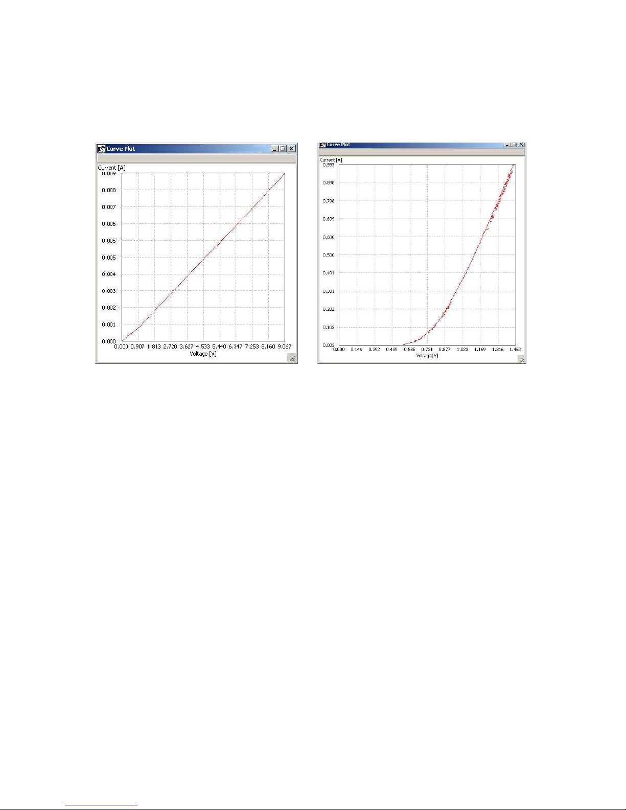
Electronic devices are useful because they cause a specific relationship between voltage and current. A curve
tracer displays the VI c haracteristic of these devices, leading to better understanding of their operation.
(a) Resistor, 1kΩ (b) Diode, MR851
Figure 1: VI Characteristics
As a very simple example, it’s possible to plot the VI characteristic of a resistor on a curve tracer. A resistor
plot appears as a diagonal straight line (figure 1a), the slope inversely proportional to the resistance. There are
simpler and less expensive ways of measuring resistance, but it’s useful to keep that example in mind when
viewing a VI plot.
For example, a diode allows current to flow in the forward directio n, and blocks it in the r everse direction.
As well, there is a small voltage drop across the diode when it is conducting. This voltage drop increases with
current, so th a t the voltage is a non-linear function of the current. We refer to the graph of this function as the
VI Characteristic for the forward-biased diode. Different diodes have different shaped curves. For example, the
voltage drop across a germanium diode is about 0.3 volts. Across an LED, it is 2 or 3 volts. Figure 1b shows the
VI characteristic of a 3 amp silicon power diode.
The curve tracer can also plot a family of VI Curves for NPN and PNP transistors, MOSFETs, JFETs and
many other semiconducto r devices.
Applications of a curve tracer include the following:
Education: Viewing Device Characteristics A lab exercise to measure device characteristics - such as the col-
lector curves of a transistor - helps students to retain important information about devices. It also teaches
students how to interpret the curves to determine device parameters and models.
Modelling a Device Detailed knowledge of the characteristics of a device allows one to model it for a simulation
program. For example , the characteristic of the diode in figure 1(b) can be modelled by an ideal diode in
series with a pure voltage source and resistor. The voltage source models the threshold voltage of the diode.
The resistor models the linear portion of the curve at higher currents.
Measuring the Range of a Parameter A device data sheet generally specifies the behaviour of the device under
certain conditions. The curve tracer can deter mine the behaviour under a range of o ther conditions. For
example, the datasheet of a transistor may not show its incremental collector resistance. This is readily
determined from a curve tracer plot.
1
Page 5

Testing a device t o determine if it is Functional It can be useful not only to know whether a device is func-
tional, but if it has failed, whether it is a short circuit, open circuit, or some other state.
Testing a device t o determine it meets its Specificat ions One can quickly determine whethe r a device mee ts
certain performance requirements, such as cur rent gain.
Matching Devices by Comparison In certain specialized applications it is useful to be able to match device
characteristics. For example, one wishes to use a pair of matched JFETs for the input to a low-noise
differential amplifier. The two JFETs should be matched, but a matched pair are not available commercially.
For low volume production or a one-off scientific instrument, a group of single JFETs can be sorted and
matched according to their curve-tracer measurements, and then used in pairs.
Testing a Two-Terminal Circuit Two terminal circuits, such as a constant current or constant voltage device,
can be constructed from co mponent parts. The curve tracer is ideal for measuring the properties of these
circuits. As another example, a negative resistance device (Lambda Diode) can be synthesized using two
junction FETs. The curve tracer can b e used to plot its VI characteristic.
Testing Unknown Device If you obtained a large quantity of a particular tra nsistor, it would be possible to de-
termine its princip al characteristics, such as polarity (NPN or PNP) and current gain.
Why do we need a curve tracer to determine device characteristics? Isn’t the information
in the datasheet?
The data sheet for a sem iconductor device will specify some or all of the maximum, minimum an d typical values
for some parameter. For example, the forward voltage drop of a diode will be specified a t some value of forward
current. The datasheet may also show a typical curve of forward voltage vs current. However, in the process of
electronic design and troubleshooting it’s often important to be able the exact behaviour of a given device.
For example, the forward voltage of a silicon diode is often quoted a 0.6 volts. A curve tracer shows that the
forward voltage of an MR851 diode, when conducting 1 amp of cu rrent, is actually about 1.4 volts. This would
be important to know when designing a power supply1.
2 The CTR-201 Curve Tracer
Early examples of the curve tracer instrument generally included a cathode ray disp la y, much like an oscilloscope.
AC line-operated power supplies swept the device voltages and currents, typically at a rate of 60 or 120Hz. The
instrument had many manual controls and extensive analog circuitry. These instruments were excellent for their
time, but they were large, heavy a nd expensive.
The CTR-201 system uses a completely different approach. The test hardware connects to a personal computer
via USB, and the computer runs a control program to operate this hardware. The hardware unit con tains various
controlable voltage and current so urces that actuate the device under test while measuring the voltages and currents
in the device. The measurement results are then handed back to the host PC for display, manipulation, or storage.
There are many advantages to this approach:
• The hardware can be rela tively simple, which reduces its size and cost. Where an electronics lab could
perhaps have one curve tracer that was shared by all staff or students, it is now feasible for each work
station to do its own dedicated measurements.
• The measurement algorithms are defined in software, so the capabilities of the instrument can be modified
and extended.
1
The curve tracer measures the characteristics of a specific device. For a production design where many units are to be produced, one
should use the worst case parameters of a semiconductor in the design. So you should in general not read the measurements from a curve
tracer of one particular device and use those results directly in a design. But you could use the curve tracer to ensure that a given device meets
or exceeds its datasheet specifications.
2
Page 6

• Measurements are conducted in pulsed mode. Tha t is, the measurement conditions are applied to the device
under test for a brief interval. The hardware captures the device behaviour during the measure ment interval.
The measurement conditions are then removed, allowing the device and the driver electronics to cool. This
approach minimizes the size and cost of the hardware, and allows measurements of a semiconductor device
up to and beyond its rated values.
For example, light emitting diodes are often operated in pulsed mode at peak currents well in excess of their
maximum allowable continuous current. The CTR-201 can take pulsed measurements up to a maximum of
1 ampere forward current.
The interval between me asurements automatically increases at higher currents to control the power dissipation in the device.
• Legacy instruments provided a repeditive display of the measurement curve. In the CTR-201, data is
captured in one measurement sweep, minimizing the dissipation in the device under test.
• Legacy instruments often used dissipation limiting resistors in series with the device under test. Then, as
the current was increased in the device, the voltage across the device decreased. This was a useful approach
to protect the device under test2. However, it limited the me a surement at the corner values of voltage and
current. You could measure the device at maximum voltage or current, but not both at once.
The CTR-201 contains no dissipation limiting resistances, and the current sensing resistances are small. As
a result, the device can be tested at the full limit of the cu rve tracer capabilities - about 35 volts at 1 ampere.
• Legacy instruments typically provide voltage-cur rent curves. A comp uter-based instrument like the CTR201 can provide many more modes of display and analysis, such as the variation in current gain of a BJT
over a range of operating currents, or the incremental collector resistance as a function of collector voltage.
The data can be captured and transferred to a spreadsheet or other prog ram for further analysis.
• Because the CTR-201 hardware is hosted by a computer it is straightforward to capture screen shots, save
the data to a file for further analysis, or project the screen image in a teaching environment.
2
As well, the voltage across the dissipation resistance could be used as a measurement of the current through the device.
3
Page 7
3 Measurements
3.1 Device Connections
3.2 Instrument Overview
A typical control panel configuration is shown in figure 2. Some sections of this display change according to
the type of device under measurement.
Here we list the various functions on the contr ol panel of the Curve Tracer. These are the functions that apply
to all measure ments.
Menu Bar: File
Save Preset Saves the current control settings.
Load Preset Loads the previously saved contr ol settings.
Menu Bar: View
Trace Smoothing Enable and disable dot connection algorithm that smooths the trace. Disable to see the actual
measurement points.
Figure 2: Typical Control Panel
4
Page 8

Menu Bar: Tools
Calibration Provides access to the calibration facility of the curve tracer. You will need multiple digital volt-
meters and ammeters to complete this process. Extreme caution is r equired.
Menu Bar: Data
Save, load and clear reference trace. This allows saving and displaying a trac e for com parison purposes.
Menu Bar: Hardware
Connect Provides access to the routine for connecting to a USB port on the host computer.
Pulsed VI Measurements When enabled, the measurements include a ’cooling’ period between each measure-
ment to minimize dissipation in the device under test.
Menu Bar: Help
Manual Accesses this doc ument.
Change Log Accesses the software changes with this version of the software.
About States the version number of the software.
Firmware Upgrade The firmware is the code installed in the hardware unit. It is not the computer code that runs
on the host computer. Forces an upgrade to the firmware. Do not access this unless a firmware upgrade is
essential. An internet connection is required of the host computer.
Check for firmware upgrades on startup Recommended to leave this enabled. To upgrade the firmware, an
internet connection is required of the host computer.
Device Status
Temperature Shows the internal temperatu re of the instrument.
USB Voltage Displays the voltage supplied by the USB connection. Should be ar ound 5 volts.
Input Voltage When taking a measurement, shows the supply voltage from the AC adaptor. Should be around
48 volts.
Device Safety
These controls allow the operator to set the current limit or the power limit for the device under measurement. If
the instrument tries to exceed this value, it stops mea surement and post a warning message.
Current Range
Allows selection of the current measurement range. There are four settings: Auto, 1 amp, 30mA, 1mA. If you
select Auto, the instrument will try to select the optimal measurement range. There will be seen a small glitch in
the trace when switching between ranges. Also, Auto can fail under certain situations, in which case a manually
selected range is necessary.
Select Device
Allows selection of the type of device under measurement. These selections can be used for other purposes as
well. For example, the N-Cha nnel JFET setting has also been used for measuring MESFETs and Russian Vacuum
tubes.
5
Page 9
Voltage-Mode, Current Mode
The VI measurement setting allows one to set the measurement mode. In Voltage mode, the instrument adjusts
the terminal voltage and measures the current. In current m ode, the instrument adjusts the current and measures
voltage. For example, in a diode-like device, when measured by voltage mode the current increases very rapidly
after the device threshold is reached. It’s much more controllable to operate the in current mode, ie, adjust the
measurement current and report the device voltage
Control Settings
These entry boxes set the parameters for a measurement. Move the cursor to the entry box a nd left click to place
the cursor in the entr y box. Then edit the value. Carriage return is not required. When you click on START,
the instrument software will read the values in these boxes. Usually some experimentation is required to get the
desired curve.
Curve Data
This section of the control panel logs the measured values as they are completed. The ’Save CSV’ function (see
above) copies this data to a .CSV file.
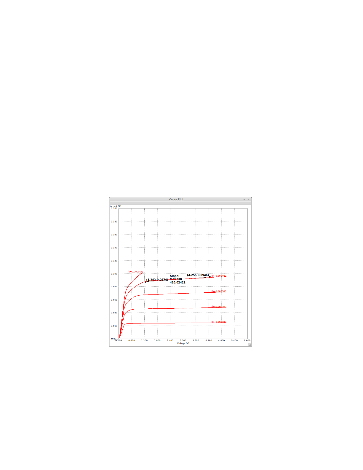
Measurement Cursors
A left click in the plot area deposits a measurement point and shows the coordinates of that point.
A second left click deposits a second point, whic h shows the coordinates of that point. The second point also
generates a line between the two points, a readout of the slope, and a reado ut of the inverse of the slope. This
provides a semi-automatic method of determining incremental conductance and resistance.
For example, in figure 3 the operator has deposited two measurement points on one of the collector characteristic curves. The collector incremental resistance is 420 ohms. This is useful infor mation for building a model of
the transistor for circuit analysis or simulation.
Figure 3: Cursors
6
Page 10
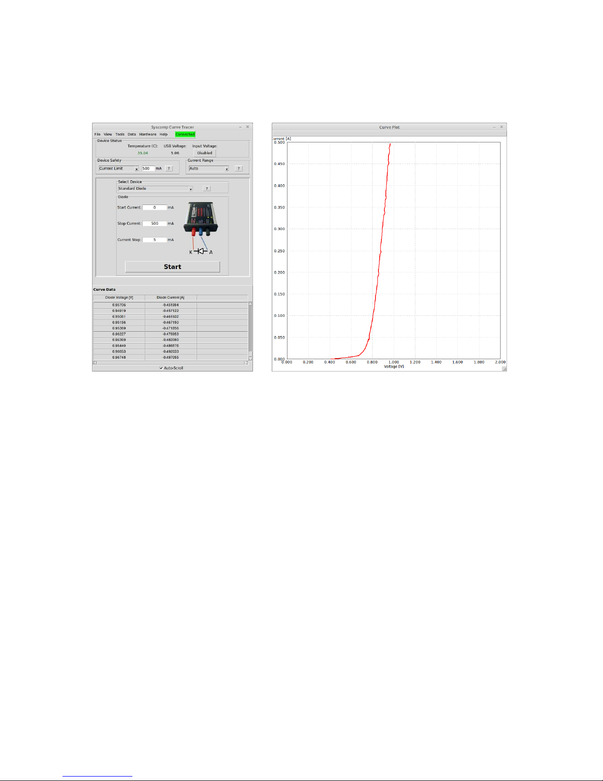
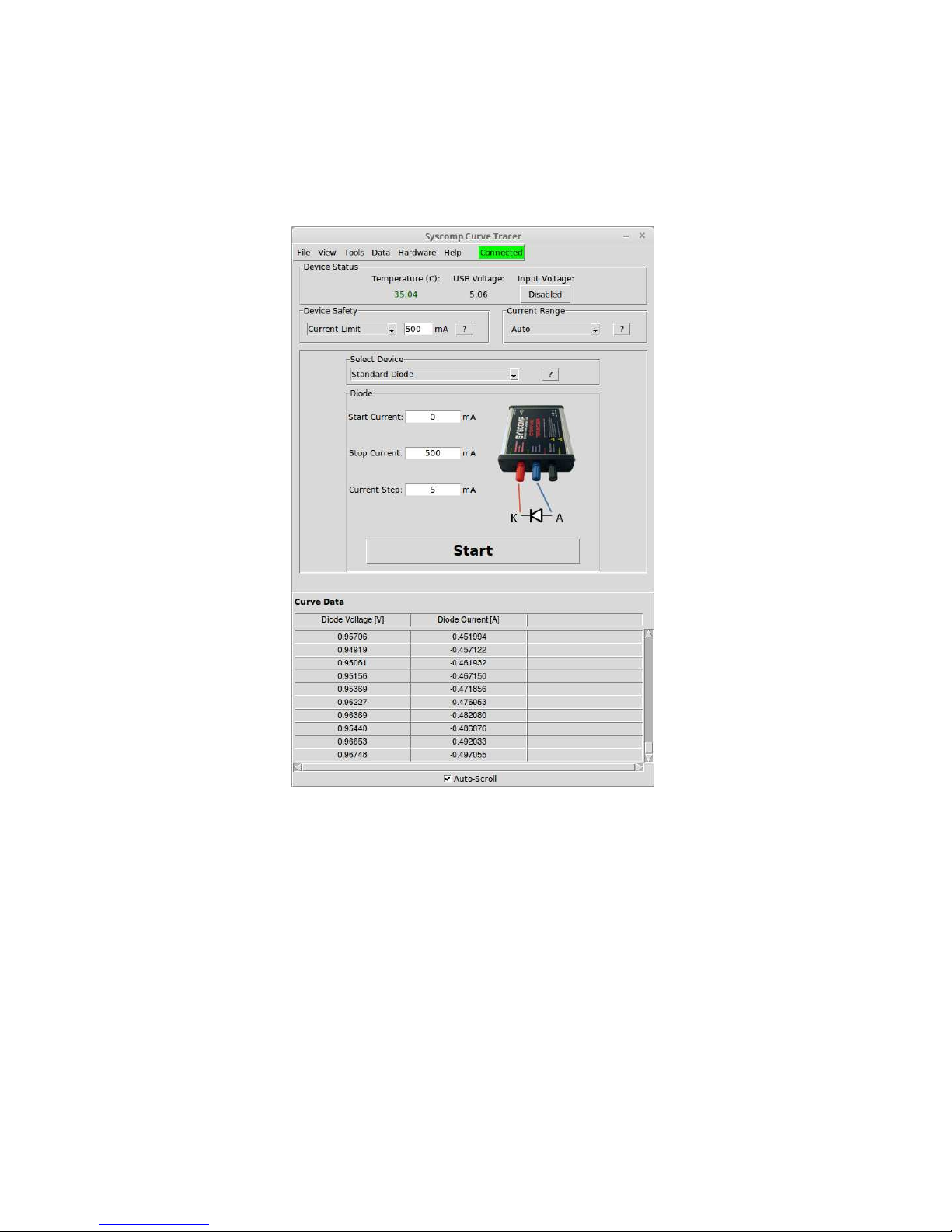
3.3 Diode
The control settings for a typical diode measurement, and the results of that measurement, are shown in figure 4.
(a) Control Settings (b) Result
Figure 4: Diode
A diode VI characteristic could be measured by placing a voltage between its terminals and measuring the
current (voltage-driven), or passing a current through it and measuring the terminal voltage (current-driven).
Either one will work, but current incr eases very rapidly with voltage once the voltage exceeds the threshold for a
diode. Conversely, forward voltage increases very slowly with cu rrent, so a current-driven measurement is more
controllable and precise.
The current source/sink is available at the centre (Blue) terminal. For the Diode measurement, the software
selects sourcing of current from that terminal. The left (Red) terminal acts as a constant voltage so urce for return
for the cur rent.
3.4 Zener Diode
The zener diode should be measured using the Diode measurement con figuration, which is current-controlled.
Figure 5 shows the characteristics of a 1N3022 zener diode. Figur e 5(a) is the forward characteristic, which
is similar to the forward characteristic of any silicon diode.
Figure 5(b) shows the reverse characteristic. The inverse of the slope of this ch aracteristic is the zener incremental resistance. The 1N3022 is billed as a 12 volt zener. The measurement shows it is more like 10 volts,
highlighing the importance of a curve tracer measurement to verify a device characteristic.
7
Page 11
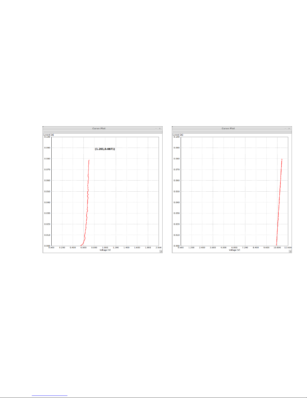
(a) Forward (b) Reverse
Figure 5: 1N3022 Zener Diode
8
Page 12

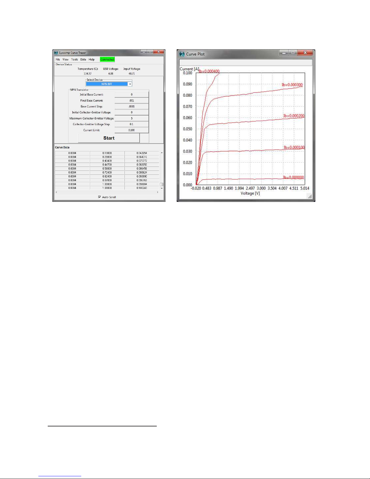
3.5 NPN Transistor (BJT)
The control settings for an NPN Power Transistor (2N3055), and the results of that measurement, a re shown in
figure 6.
(a) Control Settings (b) Result
Figure 6: NPN Transistor
Notes
• The collector current of a BJT is more-or-less constant with increasing collector-emitter voltage. That
is, it behaves as a current source (or, more accurately, a current sink in the case of an NPN transistor.)
Consequently, it is best to test this characteristic by setting a base current, sweeping the collector-emitter
voltage and measuring the collector current. The base terminal is supplied with a curren t that increases
stepwise with each sweep.
• The measurement can generate considerable power in the transistor. For example, at a test collector-emitter
voltage of 30 volts and collector current of 1 ampere, the transistor dissipation is 30 watts. A small signal
transistor might have a maximum power dissipation of 0.5 watts. Co nsequently, it’s very easy to destroy a
transistor by exceeding the power dissipation. To prevent this:
– While learning how to operate the curve tracer, use a power transistor as the device. The 2N3055 is a
good choice, since it is inexpensive, readily available, has a large semico nductor chip and is mounted
in a metal TO-3 housing.
– Do a rough calculation of the maximum expected current in the transistor. The collector current is
controlled by the base current times the current gain (DC beta β, or h
). A typical value for β
F E
is 50. Consequently, a maxim um base current of 1mA will cause a maximum collector current of
50mA. With a maximum collector-emitter voltage of 5 volts, the ma ximum dissipatio n is 250mW. For
example, a 2N4401 in a TO-92 case can dissipate around 500mW at ambient air temperature of 40◦C,
so this measurement should be safe on a 2N4401.
9
Page 13

– Use the Current Limit or Power Limit setting to protect the tran sistor from excessive current.
If the collector current tries to exceed this value, the measurement halts and the measurement currents
and voltages are removed.
– Because the measurement is pulsed with time between each pulse, it may be possible to exceed the
actual power dissipation of the device without destroying it. This is however not guaranteed, and
should be approached very carefully - or with a stack of spare devices.
3.6 PNP Transistor (BJT)
(a) Control Settings (b) Result
Figure 7: PNP Transistor
For a PNP transistor, setup and operation of the curve tracer is similar to the NPN BJT transistor, section 3.5,
page 9.
The control settings for an PNP Power Transistor (TIP32C), and the results of that measurement, are shown
in figure 7.
As mentioned in section 3.5, one must exercise caution no t to destroy the PNP device under test b y excessive
current or power dissipation.
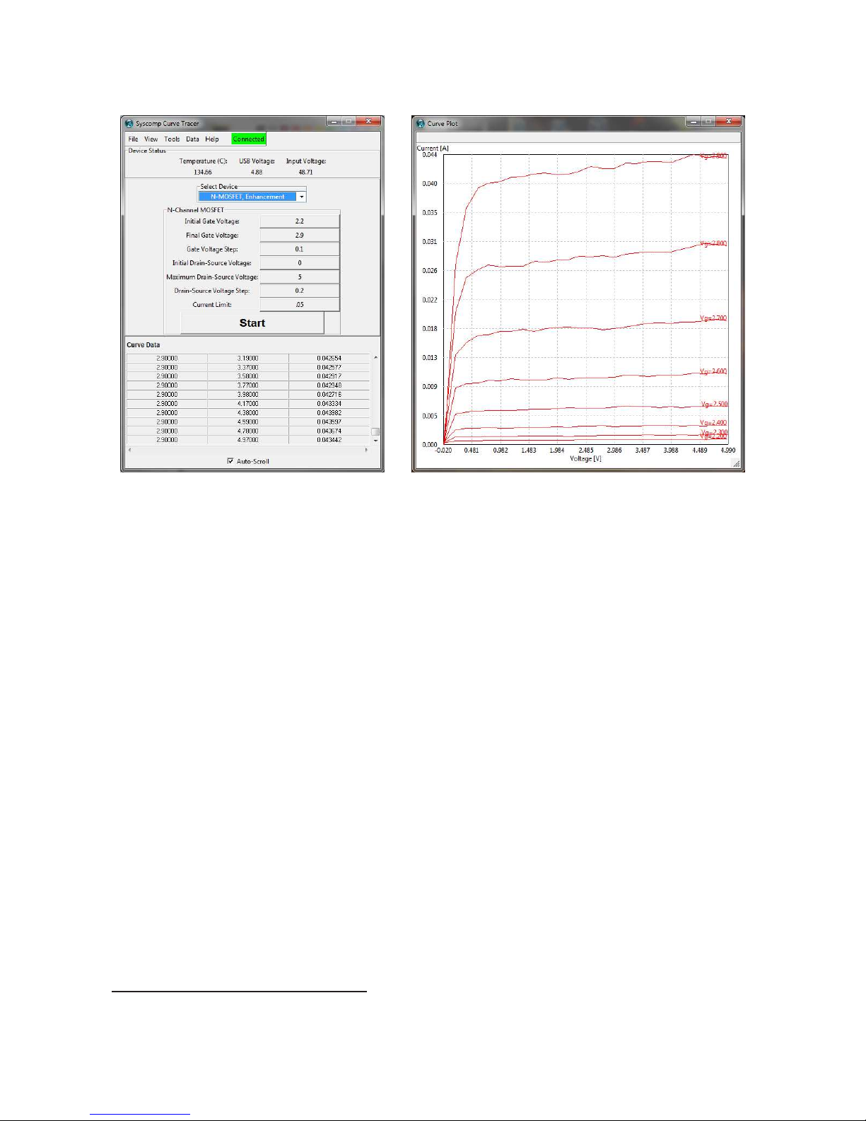
3.7 N-Channel MOSFET
The control settings for an N-Channel MOSFET (IRF820), and the results of that measurement, are shown in
figure 8.
Notice that the MOSFET drain current is essentially zero when the gate-source voltage is less than the thresh-
old voltage. It then increases very rapidly as Vgs is increased.
Like the BJT, the drain current of a MOSFET is more-or-less constant with increasing drain-source voltage.
That is, it behaves as a current source (or, more accu rately, a current sink in the case of an N-MOSFET).
Internally, the gate-source voltage originates with the same circuit that generates base current for a BJT. A
4k7Ω resistor is switched between the current gen erator and ground, converting it into a voltage source with
10
Page 14
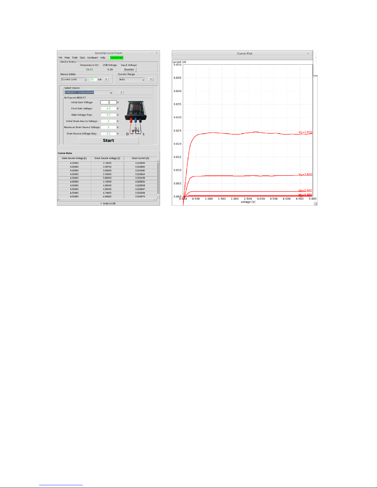
(a) Control Settings (b) Result
Figure 8: N-Channel MOSFET
an internal impedance of 4k7Ω. (The DC impedance of a MOSFET gate is essentially infinite, so the internal
impedance of this voltage source is inco nsequential.)
3.8 P-Channel MOSFET
For an P-Channel MOSFET, setup and operation of the curve tracer is similar to the N-Channel MOSFET, described previously.
3.9 N-Channel JFET
The control panel settings and a typical result are shown in figure 10.
For the JFET, the value of Idss (drain current with zero gate-source voltage) is often of interest. This can
be obtain fr om the VI plot. However, to eliminate any possible voltage between gate and source, it’s useful to
connect only the source and drain terminals to the curve tracer, as in figure 10. The gate terminal is connected to
the source terminal of the JFET, and not connected to the curve tracer. Now the characteristic curve will show the
drain voltage-current characteristic with zero Vgs.
11
Page 15
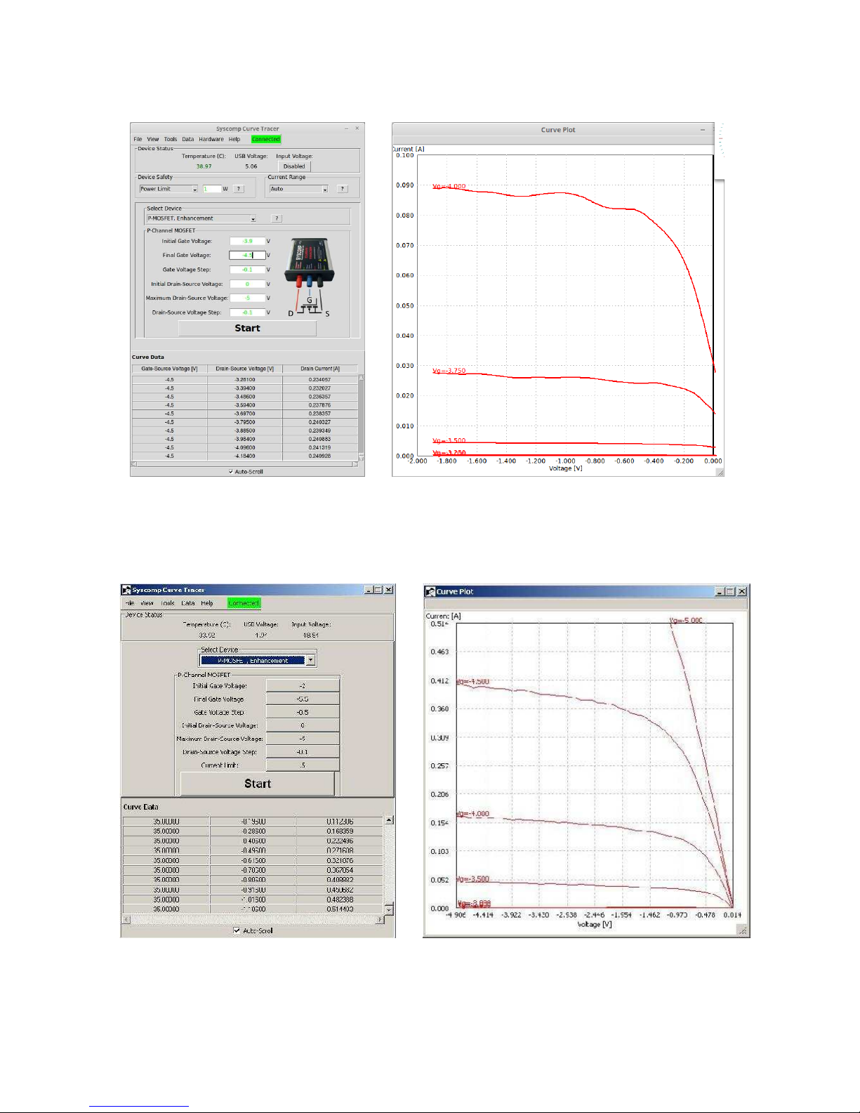
(a) Control Settings (b) Result
Figure 9: P-Channel MOSFET
(a) Control Settings (b) Result
Figure 10: N Channel JFET
12
Page 16

3.10 General 2-Terminal Measurement
For general voltage-stimulus measurement, use the 2-Terminal setting.
This measurement operates in voltage mode, where the voltage is adjusted and the current measured, and
current mode, wher e the current is adjusted and the device voltage measured.
3.10.1 2-Terminal Measurement, Voltage Mode
This measurement is capable of sweeping from a negative to positive voltage while plotting the device current, so
that all quadrants are visible.
The total rang e of voltage is 30 volts, that is:
Stop voltage − Start Voltage <= 30V
For example, the range could be set as −15V to +15V, or −5V to +25V.
(a) Control Settings (b) Result
Figure 11: 2-Terminal Measurement, Voltage Mode
A typical measurement is shown in figure 11. The device under test is an arrangement of diodes: two of
1N4001 diodes in series, in parallel with a further three 1N4001 diodes in series. The result is a device with
approximately 1.4 volt threshold in one direction and a 2.1 volt threshold in the other direction.
This test is voltage driven. Testing a constant voltage device such as a diode or zener can easily result in a
measured current that excee ds the maximum curre nt setting. In that case, a warning window will pop up. Reduce
the test voltage and then try the measurement again. For example, in the case of the diode array, a starting voltage
of -3 volts resulted in excessive current. The starting voltage was reduced to -1.8 volts, which allowed the analysis
to run to completion.
For a device with a very constant voltage drop - such as a zener with 6 volt or greater breakdown - it may be
necessary to use the current mode configuration. That configuration forces and controls the device current while
measuring the device voltage so there is less likelyhood of an over-current being triggered.
The connections ar e different for 2-terminal voltage and current mode. The instrument warns of this when
switching from voltage and current modes.
13
Page 17

3.10.2 2-Terminal Measurement, Current Mode
This measurement is similar to the 2-term inal voltage mode, with the difference that the current is controlled and
the voltage measured. The maximum range of current is +/-1 amp and the re sultant voltage +/-40V.
Notice that the device connections are different for voltage and current mode. A warning dialog pops up
when switching between them.
Figure 12 shows the previously describe d diode array measured in current mode.
(a) Control Settings (b) Result
Figure 12: 2-Terminal Measurement, Current Mode
3.11 Small Signal Transistors
In th e following images we show the control settings and curves for three small-signal devices: 2N4401 NPN BJT
(figure 13, page 15), , 2N4403 PNP BJT (figure 14, page 16) and 2N7000 N-Channel MOSFET (figure 15, page
17). All these devices are packaged in a TO-92 package and are very limited in d issipation.
These settings and results will be useful in providing a starting point for setting the controls for other smallsignal devices.
3.12 Solar Cells
The 2-terminal VI curve control panel for measur ing solar cells is shown in figure 16(a) on page 18. The solar cell
is connected with its positive ter minal to the collector (red) terminal of the curve tracer. The solar cell negative
terminal is connected to the emitter (black) termina l of the curve tracer.
A typical curve is shown in figur e 16(b) on page 18.
At zero terminal voltage the cell is delivering Isc, the short-circuit curren t, about 2.9 milliamps. At zero output
current, the cell is delivering Eoc, it’s open circuit voltage, around 5.9 volts. The intersection of the curve with the
vertical (current) axis is Isc, the short-circuit current. This varies with light level. The intersection of the curve
with the horizontal (voltage) axis is Eoc, the open-circuit voltage.
14
Page 18
(a) Control Settings (b) Result
Figure 13: 2N4401 NPN BJT
The m ove the cursor into the curve area and the cursor display then shows the voltage and current at the cursor
position.
3.13 Lambda Diode, Negative Resistance Device
The lambda diode is a circuit that behaves as a negative resistance over part o f its VI characteristic. The circuit
and characteristic are shown on pages 18 and 19.
From the literature3, we expect the shape of the curve to have a peak, followed by a valley, followed by a
rising portion. Should we test this using a current source or voltage source?
A current source creates a load line that is horizontal, so varying the test current causes this horizon ta l line to
change it’s vertical position. This load line can intersect with the VI characteristic simultaneously at as many as
three points, which leads to an ambiguous result.
A voltage source creates a load line that is vertical and changes its horizontal position. This load line can
intersect with the VI characteristic a t one point only, so the result is unambiguous.
Consequently, the device should be driven by a constant voltage source, while measuring the current. In the
CTR-201, that implies connecting it between the collector (Red) and emitter (Black) terminals, which are both
voltage sources. The current drive (Blue) terminal is not used.
This is similar to the test method for an NPN BJT and N-Channel MOSFET, where the c haracteristic is tested
by applying a voltage and measuring the current.
3.14 Vacuum Tube
Figure 19 on page 19 shows the it plate characteristic of a low-voltage vacuum tube, Russian type 1zh18b. The
vacuum tube o perates in a similar manner to an N-Channel JFET, and so the JFET setting was used on the curve
tracer. An external power supply of 1.2 volts was a lso required to power the filament in the tube.
3
Google Lambda Diode and negative resistance.
15
Page 19

(a) Control Settings (b) Result
Figure 14: 2N4403 PNP BJT
4 How It Works
A block diagram of the curve tracer is shown in figure 20. I t consists of two programm able voltage sources and
one programmable bidirectional current source. These sources are controlled by 12 bit D/A converters.
The m easured voltages and currents are shown conceptually on the diagram as voltmeters and ammeter. These
are actually A/D converter inputs that are 12 or 16 bit resolution.
By convention, the three terminals are labelled Collector, Base and Emitter, which refers to the connections for a BJT (transistor). For a MOSFET, the corresponding terminals are Drain, Gate and Source.
The curve tracer can perform mea surements on a wide variety of semiconductors besides these two devices.
Notice that a ground terminal is not available to the outside world. Measurements are perf ormed between the
three terminals.
The base current generator actually consists of two current sources. I
terminal. I
accepts current into the Base terminal. At any given time, only one of these sources is active. The
sink
compliance of the current source is equal to the full voltage range of measurements, about 42 volts.
In addition to the circuitry sh own in figure 20, the unit includes:
• Case temperature sen sor, to monitor the temperature of the metal case and shu t down supplies if the temperature becomes excessive.
– The temperature warning threshold is indicated by the temperature readout changing to an orange
colour at 45◦C.
– The software critical temperature is 50◦C. Above that temperature the software will not run.
– The firmware critical temperature is 52◦C. Above that temperature the firmware will disable the out-
puts.
supplies current out the Base
source
• Voltage monitors for the 5 VDC USB supply and 48 VDC main supply.
16
Page 20
(a) Control Settings (b) Result
Figure 15: 2N7000 N-Channel MOSFET
• Indicator LEDs. From left to rig ht these are:
Green USB Power ON.
Red 48V Power ON
Flashing Red Communications traffic.
Amber Status. Illuminates when a measurement is in progress. Flashes to indicate over-temperature con-
dition.
The hardware microprocessor accepts co mmands from the host to set the various D/A converters and acquire
various measurements. It then sends the acquired data to the host, for display and storage.
Commands are in the form of ASCII strings, so it is quite straig htforward for some other software to control
the CTR-201 hardware.
Example: Diode Measurement
A diode is connected with the anode connected to the Base terminal and the cathode to Collector terminal.
The base current source forces current through the d iode. The ammeter in the Co llector circuit measures this
current4. The voltage across the diod e is equal to the base voltage reading minus the collector voltage reading.
Example: PNP Transistor Measurement
The PNP transistor is connected to the like-named terminals on the curve tracer. The emitter and collector voltage
sources are raised to some positive voltage. The base current gene rator is configured to sink the first value of base
current. The collector voltage is then swept downward so that the emitter is more positive than th e collector and the
4
The diode current is known from the current source setting, which is quite accurate, so the collector current measurement is redundant.
However, the collector current measurement is very precise, with high resolution, so we use that.
17
Page 21

(a) Control Panel (b) VI Characteristic
Figure 16: Solar Cell
Red Blue Black
.......
..
..
.
.
.
.
.
.
.
.
.
.
.
.
.
.
.
.
.
.
.
.
.
.
.
.
.
.
.
.
.
.
.
.
.
.
.
.
.
.
.
.
.
.
.
.
.
.
.
.
.
.
.
.
.
.
.
.
.
.
.
.
.
.
.
.
.
.
.
.
.
.
.
.
.
.
.
.
.
.
.
.
.
.
.
.
.
.
.
.
.
.
.
.
.
.
.
.
.
.
.
.
.
.
.
.
.
.
.
.
.
.
.
.
.
.
.
.
.
.
.
.
.
.
.
.
.
.
.
.
.
.
.
.
.
.
.
.
.
.
.
.
.
.
.
.
.
.
.
.
.
.
.
.
.
.
.
.
.
.
.
.
.
.
.
.
.
.
.
.
.
.
.
.
.
.
.
.
.
.
.
.
.
.
.
.
.
.
.
.
.
.
.
.
.
.
.
.
.
.
.
.
.
.
.
.
.
.
.
.
.
.
.
.
.
.
.
.
.
.
.
.
.
.
.
.
.
.
.
.
.
.
..
..
.......
.
.
.
.
.
.
.
.
.
.
.
.
.
.
.
.
.
.
.
.
.
.
.
.
.
.
.
.
.
.
.
.
.
.
.
.
.
.
.
.
.
.
.
.
.
.
.
.
.
.
..
.
.
.
.
.
.
.
.
.
.
.
.
.
.
.
.
.
.
.
.
.
.
.
.
.
.
.
.
.
.
.
.
.
.
.
.
.
.
.
.
.
.
.
.
.
.
.
.
.
.
.
.
.
.
.
.
.
.
.
.
.
.
.
.
..
.......
.......
..
.
.
.
.
.
.
.
.
.
.
.
.
.
.
.
.
.
.
.
.
.
.
.
.
.
.
.
.
.
.
.
.
.
.
.
.
.
.
.
.
.
.
.
.
.
.
.
.
.
.
.
.
.
.
.
.
.
.
.
.
.
.
.
.
.
.
.
.
.
.
.
.
.
.
.
.
.
.
.
.
.
.
.
.
.
.
.
.
.
.
.
.
.
.
.
.
.
.
.
.
.
.
.
.
.
.
.
.
.
.
.
.
.
.
.
.
..
....
.
.
.
.
.
.
.
.
.
.
.
.
.
.
.
.
.
.
.
.
.
.
2N3810
.......
..
..
.
.
.
.
.
.
.
.
.
.
.
.
.
.
.
.
.
.
.
.
.
.
.
.
.
.
.
.
.
.
.
.
.
.
.
.
.
.
.
.
.
.
.
.
.
.
.
.
.
.
.
.
.
.
.
.
.
.
.
.
.
.
.
.
.
.
.
.
.
.
.
.
.
.
.
.
.
.
.
.
.
.
.
.
.
.
.
.
.
.
.
.
.
.
.
.
.
.
.
.
.
.
.
.
.
.
.
.
.
.
.
.
.
.
.
.
.
.
.
.
.
.
.
.
.
.
.
.
.
.
.
.
.
.
.
.
.
.
.
.
.
.
.
.
.
.
.
.
.
.
.
.
.
.
.
.
.
.
.
.
.
.
.
.
.
.
.
.
.
.
.
.
.
.
.
.
.
.
.
.
.
.
.
.
.
.
.
.
.
.
.
.
.
.
.
.
.
.
.
.
.
.
.
.
.
.
.
.
.
.
.
.
.
.
.
.
.
.
.
.
.
.
.
.
.
.
.
.
.
.
..
..
.......
s s
....
.
.
.
.
.
.
.
.
.
.
.
.
.
.
.
.
.
.
.
.
.......
.
MPF102
Figure 17: Lambda Diode
collector-emitter voltage moves over the range demanded by the software. During the sweep, the microprocessor
captures the collector-emitter voltage and collector current readings and sends them to the host. The base current
generator then steps to its next base current and the voltage sweep repeats.
18
Page 22

(a) Control Settings (b) Result
Figure 18: Lambda Diode
Figure 19: Vaccum Tube
19
Page 23

Isink
......
..
.
.
.
.
.
.
.
.
.
.
.
.
.
.
.
.
.
.
.
.
.
.
.
.
.
.
.
.
.
.
.
.
.
.
.
.
.
.
.
.
.
.
.
A
.
.
.
.
.
.
.
.
.
.
.
.
.
.
..
.
..
.
.
.
.
.
.
.
.
.
.
.
.
.
.
.
.
.
.
.
.
.
.
.
.
.
.
.
.
.
.
.
.
.
.
.
.
.
.
.
.
.
.
.
.
.
.
.
.
.
.
.
.
.
.
.
.
.
.
.
.
.
.
.
.
.
.
.
.
.
.
.
.
.
.
.
.
.
.
.
.
.
.
r
.
.
.
.
.
.
.
.
.
.
.
.
.
.
.
.
.
.
.
.
.
.
.
.
...
.
..
.
.
.
.
.
.
.
.
♣
.
.
.
♣
.
.
.
♣
.
.
.
♣
.
.
♣
.
.
.
♣
.
.
.
r
♣
.
♣
.
.
.
♣
.
.
.
♣
.
.
.
♣
.
.
.
♣
.
♣
.
.
.
♣
.
.
.
♣
.
.
.
.
.
.
.
.
.
.
.
.
.
.
.
.
.
.
.
.
.
..
...
Collector
.
.
.
.
....
....
..
.
.
..
.
.
.
.
.
.
.
.
.
.
.
.
.
.
.
.
.
.
.
.
.
.
.
.
.
.
.
.
.
.
.
.
.
.
.
.
.
.
.
.
.
.
.
.
.
.
.
.
.
.
.
.
.
.
.
V
.
.
.
.
.
.
.
.
.
.
.
.
.
.
.
.
.
.
.
.
.
.
.
.
.
.
.
.
..
..
.....
Collector Voltage Drive
Vo +3.15V to +42V, minimum step 9.5mV
Collector Current Measured
Low Range: 100nA to 1mA, resolution 15nA (16 bit)
.
.
.
.
.
.
.
.
.
.
.
.
High Range: 100uA to 1A, resolution 15uA (16 bit)
Collector Voltage Measured
0 to 42 volts, resolution 11mV
....
.
.
.
.
.
.
.
.
♣
.
.
♣
.
.
♣
.
.
♣
.
.
♣
.
.
♣
rrr
.
.
.
.
.
.
.
.
.
.
.
Current
r
.
.
.
.
.
.
.
.
.
.
.
.
.
.
.
.
.
.
..
.
.
.
.
.
.
.
.
.
.
..
.
.
.
.
.
.
.
.
.
.
.
.
.
.
.
.
.
.
.
.
.
.
.
.
.
.
.
.
.
.
.
.
.
.
.
.
.
.
.
.
.
.
.
.
.
.
.
.
.
.
.
.
.
.
.
.
.
.
.
.
.
.
.
.
.
.
.
.
.
.
.
.
.
.
.
.
.
.
.
......
.
.
.
.
.
.
.
.
.
.....
......
.
.
.
.
.
.
.
.
.
.....
r
.
.
..
.
.
4k7
.
.
..
.
.
.
.
.
.
.
.
.
.
.
.
.
.
.
.
.
.
.
.
.
.
.
.
.
.
.
.
.
.
.
.
.
.
.
.
.
.
.
.
.
.
.
.
.
.
.
.
.
.
.
.
.
.
.
.
.
.
.
.
.
Voltage
.
.
....
.
.
.
.
.
.
.
.
.
.
.
.
.
.
.
.
.
.
.
.
.
.
.
.
.
.
.
.
.
.
.
.
.
.
.
.
.
.
.
.
.
.
.
.
.
.
.
.
.
.
.
.
.
.
.
.
.
.
.
.
.
.
.
.
.
.
.
.
.
.
.
.
r
.
.
.
.
.
.
.
.
.
.
.
.
.
.
.
.
.
.
.
.
.
.
.
.
.
.
...
..
..
.
.
.
.
.
.
.
.
.
.
.
.
.
.
.
.
.
.
.
.
.
.
.
.
.
.
.
.
.
.
.
.
.
.
.
.
.
.
.
.
.
.
.
.
.
.
.
.
.
.
.
.
.
.
.
.
.
.
.
.
.
.
.
.
.
.
.
.
.
.
.
.
.
.
.
.
.
.
.
.
.
.
.
.
.
.
.
.
.
.
.
.
.
.
.
.
.
.
.
.
.
.
.
.
.
.
.
.
.
.
.
.
.
.
.
.
.
.
.
.
.
.
.
....
.
.
.
.
.
.
.
.
.
.
.
.
.
.
.
.
.
.
.
.
.
.
.
.
.
.
.
.
.
.
.
.
..
.
.
.
.....
.
.
.
.
.
.
.
.
.
.
.
.
.
.
.
.
.
.
.
.
.
.
.
.
.
.
..
.
Isource
..
.
.
.
.
.
.
.
.
.
.
.
.
.
.
.
.
.
.
.
.
.
.
.
.
.
.
.
.
.
......
.
..
.
.
.
.
.
.
.
.
.
.
.
.
.
.
.
.
.
.
.
.
.
.
.
.
.
.
.
.
.
....
.
.
.
.
.
.
.
.
.
.
.
.
.
.
.
.
.
.
.
.
.
.
.
.
.
.
.
.
.
.
.
.
.
.
.
.
.
.
.
.
.
.
.
.
.
.
.
.
.
.
.
.
.
.
.
.
.
.
.
.
.
.
.
.
.
.
.
.
.
.
.
.
.
.
.
.
.
.
.
.
.
.
.
.
.
.
.
.
.
.
.
.
.
.
.
.
.
.
.
.
.
.
.
.
.
.
.
.
.
.
.
.
.
.
.
.
.
.
.
.
.
.
.
.
.
.
.......
.
.
.
.
.
.
.
.
.
.
r
.
.
.
.
.
.
.
.
.
.
.
.
.
.
.
.
.
.
.
r
♣
.
♣
.
.
♣
.
.
♣
.
.
♣
.
♣
.
.
♣
.
.
♣
.
.
♣
.
.
.
.
.
Base
.
.
.
.
.
...
......
..
.
.
.
.
.
.
.
.
.
.
.
.
.
.
.
.
.
.
.
.
.
.
.
.
.
.
.
.
.
.
.
.
.
.
.
.
.
.
.
.
.
.
.
.
.
.
.
.
.
.
.
.
.
.
.
.
.
V
.
.
.
.
.
.
.
.
.
.
.
.
.
.
.
.
.
.
.
.
.
.
.
.
.
.
.
.
.
.
..
..
...
Base Current Drive
Low range: +/-2uA to 10mA, minimum step 2uA
High range: +/-200uA to 1A, step 200uA
Base Voltage Drive
0 to 47 volts, minimum step 9.4mV
Base Voltage Measured
0 to 47 volts, resolution 700uV
....
.
.
.
.
.
.
.
.
♣
.
.
♣
.
.
♣
.
.
♣
.
.
♣
.
.
♣
.
r
♣
.
♣
.
.
♣
.
.
♣
.
.
♣
.
♣
.
.
♣
.
.
♣
.
.
♣
.
.
.
.
.
.
Emitter
.
.
.
.
...
......
..
.
.
.
.
.
.
.
.
.
.
.
.
.
.
.
.
.
.
.
.
.
.
.
.
.
.
.
.
.
.
.
.
.
.
.
.
.
.
.
.
.
.
.
.
.
.
.
.
.
.
.
.
.
.
.
.
.
.
.
V
.
.
.
.
.
.
.
.
.
.
.
.
.
.
.
.
.
.
.
.
.
.
.
.
.
.
.
.
..
..
...
.
.
.
.
.
.
.
.
Emitter Voltage Drive
Vo +3.15V to +42V, minimum step 9.5mV
Emitter Voltage Measured
0 to 42 volts, resolution 11mV
Figure 20: Curve Tracer Block Diagram
20
Page 24

5 Calibration
(a) Ground Point
(b) Attaching to Ground
Figure 21: Attaching to the Ground Point
21
Page 25

The curve tracer is supplied in calibrated form. It shouldn’t be necessary to do a re-calibration, but we supply the
information in this section.
The curve tracer should not be opera ted in the uncalibrated state. It will generate incorrect results and may
cause damage.
You will need a digital multimeter with voltage and cu rrent ranges and an alligator clip lead. The multimeter
should have voltage resolution of 1mV or better and 0.01mA or better.
• Remove rear panel of the curve tracer.
• In the right corner, next to the USB connector, there is a square area marked on the PC board, shown in
figure 21(a) on page 21. This is the ground point for the instrument. Attach an alligator clip lead to that
point as shown in figure 21(b).
• Plug in the power adaptor and the USB cable to the instrum ent. Start the curve tracer software.
• Select the menu item Tools -> Calibration. The Calibration panel appears, similar to figure 22.
Figure 22: Calibration Panel
The Curve Tracer software assumes that the output voltages and currents, and the feedback voltages and
currents, can be corrected by a straight line equation y = M x + B. The calibration procedure establishes
the values of slope M and y offset B. It does this by outputting an assumed value (eg, 10 volts). The
operator then enters the actual output voltage. Doing this twice provides two equations in two unknowns,
so that the ac tual values o f slope M and y offset B can be determined. In general, the values of slope will
be fairly close to unity, and y offset less than unity though there can be exceptions.
• Select Reset Calibration Values. This wipes the existing calibration and you must then enter
new calibration values.
• The software has been designed as a Wizard to guide the operator through the entire calibration process.
To begin with, click on Calibrate Collector Voltage and follow the on-screen instructions. The
software outputs a voltage (eg, 10 volts) and asks for the operator to enter the actual voltage rea ding (which
might be 9.7 volts). When the software has done this twice it has enough information to calculate the slope
and y offset for the collector voltage function.
Then the software outputs a test value, such as 10 volts. The m eter reading should be very close to 10 volts.
• Continue with the other calibrations in a similar manner. Some of the calibration steps will require current
measurement.
22
Page 26

• When done, click on Save Calibration Values. The unit is now calibrated.
6 Installing the Software
6.1 Packaged Executable
The simplest method of installing the software is to run the provided installer executable for your computer. There
are three different versions of this executable, one each for the Windows, Mac and Linu x operating systems.
The installer will create the necessary directories, move files into those directories, and provide a start icon on
the desktop. Then you can r un the progra m by double-clicking on the start icon.
The latest executable can be obtained from the Downloads section of the Syscomp web page.
6.2 Source Code
The source code is the original program text. With source code, you can read how the code operates and modify
the code to suit your own purposes5.
The software has been designed to run without change under the Windows, Linux and Macintosh operating
systems. Thus there is only one version of the software source code. That makes it easy for us to maintain and
easy for you to find the right version.
Why would you want to run the software from the source code ?
Add or modify features You purchased the hardware and would like to modify the appearance or add features.
You need the source code to do so.
Education You’d like to read the code to le a rn Tcl programming.
Build another Application The source code contains routines that would be useful in your own application. The
software is provided under the Gnu Public License (GPL). Under this license, anyone may use, modify
distribute the source cod e for their own pu rposes, but cannot take the existing code private.
Protection against Obsolescence Syscomp employees are subjected to an alien abduction and no longer avail-
able. The executable installers are out of date – or for whatever reaso n, do not work. Then, if you c an ge t
the Tcl interprete r to run on your machine, you can run the instrument source code.
The source code is written in the Tcl (pronounced ’tickle’) language. Tcl is interpreted, that is, read and
executed lin e by line by the Tcl interpreter.
The Tcl interpreter is different for each operating system. You download Tcl from the Activestate website and
install the Tcl interpreter on your machine. The n you run the Tcl interpre ter and instruct it to read (source) the
Tcl source cod e files, starting with main.tcl.
6.2.1 Obtaining the Source Code
Obtain the installer executable from the Syscomp website and run it. Among other thin gs, the installer puts the
source code in a subdirectory labelled ’source’. Find the directory where the Syscomp instrument software was
installed. Open it and look for a subdirectory name d source. In that subdirectory, there should be a series of
files with the .tcl extension. These are the source code files. They can be opened and read in any text editor.
The program starts in main.tcl, w hich reads the other tcl files as it needs them.
There may also be subdirectories, such as Images and bin.6.
5
At the time of writing, Syscomp was the only oscilloscope and waveform generator company providing source code for its products.
6
Images contains various icons in image format (such as gif). bin contains the executables, for the different operating systems. These
executables are self contained - they include both the source code and the Tcl interpreter, so they can stand alone and execute on a machine.
23
Page 27

6.2.2 Installing the Tcl Interpreter on a Windows Machine
To run the source code, you need the Tcl interpreter installed on your Windows machine. The Tc l/Tk language is
not part of the Windows operating system, so it must be downloaded and installed. Fortunately, that is straightforward. Download and install Tcl/Tk for windows from the ActiveState web site: www.activestate.com/
Products/ActiveTcl Follow the installation instruc tions. At the conclusion of the installation procedure,
you should have the Tcl/Tk programming language installed and it will be visible as a new desktop icon such as
WISH84.
This only need be done once.
Now you can use the Tcl/Tk interpreter wish to execute the source code, as described in the next section . The
program should run and the instrument GUI appear. Now you can use any ed itor to modify the code, and then run
the modified code to test it.
6.2.3 Executing the Source Code
To execute the tcl source code, you can use any of the following meth ods:
• Execute the command wish main.tcl from the DOS prompt command line.
• Start the WISH interpreter and then, in the WISH console window type the command source main.tcl
• Set up a file association so that double clicking on main.tcl automatically invokes the WISH interpre te r
to execute the file. Here’s how you do that:
1. Find main.tcl in the directory that contains the source code.
2. Rig ht-click on main.tcl.
3. Ch eck that Opens With shows WISH84 (or whatever your WISH interpreter is named). If this is
not the case, then:
4. Sele c t Change. This brings up the Open With.. dialogue.
5. Sele c t Browse. This brings up a file selector dialogue.
6. N ow find the WISH84 icon on your desktop. Right click on the WISH84 icon, select Properties
to determine the location of the WISH84 program.
7. Co py that location into the previous Browse dialogue.
Now double-clicking on any file with the .tcl suffix will ca use it to be executed by WISH.
7 Commands
Cautionary Note
The CTR-201 Curve Tracer is designed to measure device characteristics by applyin g a voltage and measuring
the resultant current, or vice versa.
Using computer control, the applied voltage or current can be of very short duration. This minimizes the
dissipation in the device and in the curve tracer drive circuitry. Consequently, under normal operation, the curve
tracer c an make a sequence of measurements without significant dissipation in the drive cir cuitry. The software
enforces this by measuring the internal temperature.
When using the API commands detailed below, it is the programmer’s responsibility to ensure that the internal
dissipation is not exceeded. At large output voltage and current, there is considerable dissipation in the drive
amplifier and an excessive temperature may be the result.
The drive amplifier outputs, on the Collector and Emitter output terminals, are capable of output voltages
in excess of +10 to +40 volts, and currents of one ampere. They are not capable of continuous output at these
voltages and currents. These outputs cannot be used as power supplies for continuous output.
If you are developing custom software for a measurement application, we recommend that you use the provided source code and progra m in the Tcl language to call the various routines, or use the provided so urce code
as a guide for programming in a different language.
24
Page 28

7.1 Testing the Commands
It is possible to communicate with the CTR-201 hardware using a terminal emulator program. Under Linux,
communication was established with the CTR-201 software using the Cutecom terminal emulator.
Settings for the emulator:
Device /dev/ttyUSB0
Baud rate 115200
Data bits 8
Stop bits 1
Parity none
Handshake none
Open for Reading, Writing
7.2 Command List
i Identify Sends identification message
eg: *Syscomp Curve Tracer V1.6
E Write to EEPROM
e n Read from EEPROM address n
D set the drain/collector voltage, 12 bit value between 0 and 4096
eg: D 386
see Note.
S set the source/emitter voltage, 12 bit value between 0 and 4096
eg: S 404
see Note.
B set the upper base voltage
eg: B 348
12 bit value between 0 and 4096
Sets the ’source’ output current at the Base terminal. See note.
b set lower base voltage
eg: b 0
12 bit value between 0 and 4096
Sets the ’sink’ output current at the Base terminal. See note.
P base driver high current set point
v set Base drive mode to ’voltage’
c set Base drive mode to ’current’
r select low range (0 to 1mA) collector current sensing resistor
R select high range (0 to 1A) collec tor current sensing resistor
+ select positive collector cu rrent polarity (current out of terminal)
- select negative collector current polarity (current into terminal)
A read the 16 bit A/D converter channel 0 (Base Voltage).
a read the 16 bit A/D converter channel 1 (Collector Current).
T read the heatsink temperature
25
Page 29

eg: sends T\0x06\0x05 f or 65C
U read the USB supply voltage.
eg: returns U\0x06\0x9d
C read the collector voltage (12 bit value)
X read the emitter voltage (12 bit value)
V read the 48 volt input supply voltage.
eg: returns V\0x00\0xd6
H set high current range for base output
h set low current range for base output
G perform a high curre nt source measurement
Enables output voltage, measures resultant current.
g perform a high current sin k measurement
Enables output voltage, measures resultant current.
L turn the analysis LED on
l turn the analysis LED off
Notes
Setting external voltages accurately relies on a y=Mx+B correction in the calibration memory. Operating the
calibration control panel and observing the message traffic, we obtain the following messages for various outputs:
Collector Voltage
10V D 404
20V D 1451
40V D 3544
Emitter Voltage
10V S 404
20V S 1458
40V S 3565
Base Voltage
10V B 1090
20V B 1828
40V B 3304
Example:
h Set low current range for base output
v set Base drive mode to ’voltage’
b 0 set Sink current to zero
B 1090 set Base output voltage to 10V
The exact values of these me ssages depend on the calibration of the hardware and will vary between different
CTR-201 units. Determining the se values on your hardware gives the relationship between the command value
and the output voltage.
26
Page 30

Base Drive Circuit
The base terminal is driven from a sourcing current source and a sinking current source. The output current (out
of the base terminal) is equal to the sourcing current minus the sinking current. In practice, one or other current
source is turned off. Each current source has both a low range (100nA to 1mA) and high range (100uA to 1A).
The base voltage is created b y connecting an internal resistor of 4k7 ohms between the base termin al and ground.
Then the current source creates a voltage at the base terminal.
Upgrading to the Latest Version Software can be upgraded at any time by downloading the latest version from
the Syscomp website, in the Downloads section.
Under a Windows operating system, download a nd run the installer program. Follow the commands and the
software should install automatically.
Under a Ma c operating system, you may need to disable Gatekeeper. See: https://answers.uchicago.
edu/page.php?id=25481. Then r un the install program. Follow the commands and the software should install automatically.
Under a Linux operating system, download and unzip the distribution into a new directory. The 32 bit and 64
bit executables are included in that distribution: change the permissions and run the corresponding executable.
The source code is also provided: the executables run that sour ce code so changes to the sour ce code will be
reflected in the behaviour of the program.
If the firmware should be upgraded, the software will detect and announce that. Follow the instructions. Do
not shut off the Curve Tracer power or disconnect from the host computer until that download and installation are
complete.
7.3 Export and Import Data, Compare Measurements
Under the Data menu there are now three entries:
Export Curve Data to CSV This selection saves the measurement results to a CSV (comm a-separated-value)
file. A CSV formatted file can be read by any text editor and imported into a spreadsheet or plotting
program like gnuplot.
Load Reference Curve This selection loads and plots the data from a previously-saved CSV file as a reference
curve. T he reference cur ve is shown in black to distinguish it from a measurement trace, in red.
You can then run the measurement of another device to compare it with the reference device. Figure 23
shows the comparison of an NPN power transistor 2 N 3055 (black trace) with a small signal NPN transistor
(2N4401).
Clear Reference Curve This selection r emoves the reference curve from the plot area.
7.4 48 Volt Power Enable/Disable
A new button has been created to enable the 48 volt input power, shown as Disabled in figure 24. Under normal
operating conditions, it is not necessary to actuate this button. Simply start the analysis by a left-click on the
Start button. The Input Voltage then changes from a button to a display of the actual input voltage. Some
time after a measurement, the software disables the 48 volt supply and the readout then indicates Disabled.
When the 48 volt supply is disabled, there is a small residual voltage between the terminals of the curve
tracer, typically 3 to 5 volts, supplied through a very high source impedance. This voltage has no effect on most
semiconductors.
Clicking on the Input Voltage button enables the 48 volt su pply before taking a measurement. This ha s
the effect of activating the output amplifiers in the curve tracer, which then causes the output voltages to become
very nearly equal. The input power will remain enabled until some time after a m easurement is completed.
27
Page 31

htb
Figure 23: BJT Comparison
7.5 Pulsed VI Measurement
This option was provided to a customer to minimize power dissipation in the device under test. With this option
selected, the measuremen t of each point should be about 7.5ms long. T he curve may be a bit noisier as we are
doing less averaging in the firmware.
28
Page 32

htb
Figure 24: 48V Power Enable/Disable
29
 Loading...