


EN
SolidFlow 2.0
Solid volume measurement
Operating Instructions

Operating Instructions
TABLE OF CONTENTS Page
1. System overview . . . . . . . . . . . . . . . . . . . . . . . . . . . . . . . . . . . . . . . . . . . . . . . . . . . . . . . . . . . . . . . . . . . . . . . 3
2. Function . . . . . . . . . . . . . . . . . . . . . . . . . . . . . . . . . . . . . . . . . . . . . . . . . . . . . . . . . . . . . . . . . . . . . . . . . . . . . . 5
3. Safety . . . . . . . . . . . . . . . . . . . . . . . . . . . . . . . . . . . . . . . . . . . . . . . . . . . . . . . . . . . . . . . . . . . . . . . . . . . . . . . . 6
3.1 Normal use . . . . . . . . . . . . . . . . . . . . . . . . . . . . . . . . . . . . . . . . . . . . . . . . . . . . . . . . . . . . . . . . . . . . . . . 6
3.2 Identification of hazards . . . . . . . . . . . . . . . . . . . . . . . . . . . . . . . . . . . . . . . . . . . . . . . . . . . . . . . . . . . . 6
3.3 Operational safety . . . . . . . . . . . . . . . . . . . . . . . . . . . . . . . . . . . . . . . . . . . . . . . . . . . . . . . . . . . . . . . . . . 6
3.4 Technical statement . . . . . . . . . . . . . . . . . . . . . . . . . . . . . . . . . . . . . . . . . . . . . . . . . . . . . . . . . . . . . . . . 6
4. Mounting and installation . . . . . . . . . . . . . . . . . . . . . . . . . . . . . . . . . . . . . . . . . . . . . . . . . . . . . . . . . . . . . . 7
4.1 Typical components of the measurement point . . . . . . . . . . . . . . . . . . . . . . . . . . . . . . . . . . . . . . . . . 7
4.2 Required equipment . . . . . . . . . . . . . . . . . . . . . . . . . . . . . . . . . . . . . . . . . . . . . . . . . . . . . . . . . . . . . . . . 7
4.3 Sensor installation . . . . . . . . . . . . . . . . . . . . . . . . . . . . . . . . . . . . . . . . . . . . . . . . . . . . . . . . . . . . . . . . . 7
4.4 Mounting the transmitter . . . . . . . . . . . . . . . . . . . . . . . . . . . . . . . . . . . . . . . . . . . . . . . . . . . . . . . . . . 10
4.5 Use in hazardous areas . . . . . . . . . . . . . . . . . . . . . . . . . . . . . . . . . . . . . . . . . . . . . . . . . . . . . . . . . . . . 12
5. Electrical connection . . . . . . . . . . . . . . . . . . . . . . . . . . . . . . . . . . . . . . . . . . . . . . . . . . . . . . . . . . . . . . . . . . 13
5.1 DIN rail terminal layout . . . . . . . . . . . . . . . . . . . . . . . . . . . . . . . . . . . . . . . . . . . . . . . . . . . . . . . . . . . . 13
5.2 Field housing terminal layout . . . . . . . . . . . . . . . . . . . . . . . . . . . . . . . . . . . . . . . . . . . . . . . . . . . . . . . 14
5.3 C1-box terminal layout . . . . . . . . . . . . . . . . . . . . . . . . . . . . . . . . . . . . . . . . . . . . . . . . . . . . . . . . . . . . . 15
5.4 C3-box terminal layout . . . . . . . . . . . . . . . . . . . . . . . . . . . . . . . . . . . . . . . . . . . . . . . . . . . . . . . . . . . . . 15
6. Operator interface . . . . . . . . . . . . . . . . . . . . . . . . . . . . . . . . . . . . . . . . . . . . . . . . . . . . . . . . . . . . . . . . . . . . 16
6.1 Differences between the DIN rail and field housing transmitter . . . . . . . . . . . . . . . . . . . . . . . . . . 16
6.2 Display . . . . . . . . . . . . . . . . . . . . . . . . . . . . . . . . . . . . . . . . . . . . . . . . . . . . . . . . . . . . . . . . . . . . . . . . . . 17
6.3 PC interface . . . . . . . . . . . . . . . . . . . . . . . . . . . . . . . . . . . . . . . . . . . . . . . . . . . . . . . . . . . . . . . . . . . . . 18
6.4 One or more sensor system . . . . . . . . . . . . . . . . . . . . . . . . . . . . . . . . . . . . . . . . . . . . . . . . . . . . . . . . . 20
6.5 Menu structure . . . . . . . . . . . . . . . . . . . . . . . . . . . . . . . . . . . . . . . . . . . . . . . . . . . . . . . . . . . . . . . . . . . 21
7. Start-up procedure . . . . . . . . . . . . . . . . . . . . . . . . . . . . . . . . . . . . . . . . . . . . . . . . . . . . . . . . . . . . . . . . . . . 29
7.1 Basic start-up . . . . . . . . . . . . . . . . . . . . . . . . . . . . . . . . . . . . . . . . . . . . . . . . . . . . . . . . . . . . . . . . . . . . 29
7.2 Adjusting the measurement values . . . . . . . . . . . . . . . . . . . . . . . . . . . . . . . . . . . . . . . . . . . . . . . . . . 29
8. Maintenance . . . . . . . . . . . . . . . . . . . . . . . . . . . . . . . . . . . . . . . . . . . . . . . . . . . . . . . . . . . . . . . . . . . . . . . . . 30
9. Warranty . . . . . . . . . . . . . . . . . . . . . . . . . . . . . . . . . . . . . . . . . . . . . . . . . . . . . . . . . . . . . . . . . . . . . . . . . . . . 30
10. Troubleshooting . . . . . . . . . . . . . . . . . . . . . . . . . . . . . . . . . . . . . . . . . . . . . . . . . . . . . . . . . . . . . . . . . . . . . . 30
11. Technical data . . . . . . . . . . . . . . . . . . . . . . . . . . . . . . . . . . . . . . . . . . . . . . . . . . . . . . . . . . . . . . . . . . . . . . . 31
2

Operating Instructions
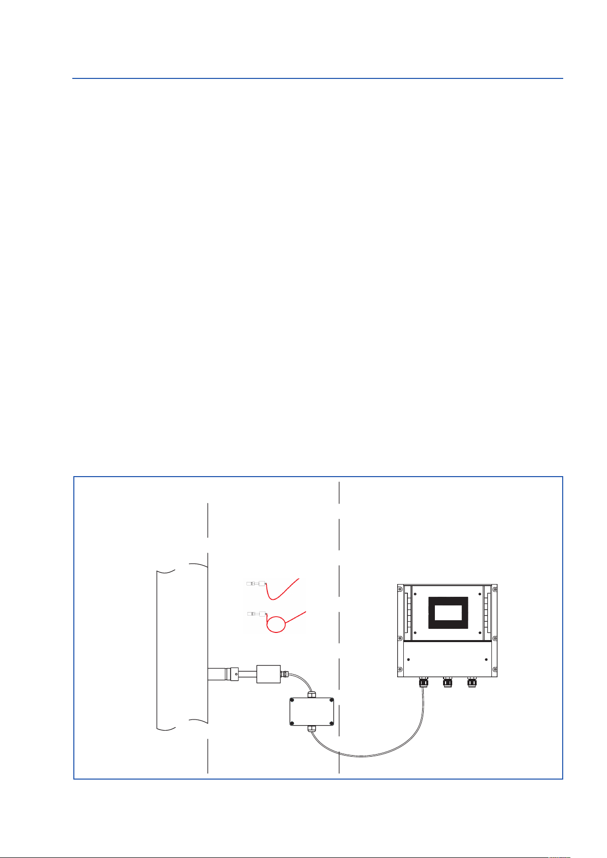
1. System overview
A measuring point consists of the following components:
• Transmitter (in the DIN rail housing or field housing)
• Sensor mount for welding to the pipeline
• Sensor (union nut, spacer rings, sealing ring for adjusting to the wall thickness)
• Installation instructions
• C1- or C3-box
Sensor
C1-Box
Sensor C1-Box Transmitter
2 m
Fig. 1: Overview with C1-box and field housing transmitter
Sensor
Sensor C1-Box Transmitter
1 (+ 24 V)
2 (GND)
3 (A)
4 (B)
S (Earth)
max. 300 m
C1-Box
16 (+ 24 V)
15 (GND)
14 (A)
13 (B)
2 m
Fig. 2: Overview with C1-box and DIN rail transmitter
max. 300 m
3

Operating Instructions
The system can be equipped with up to three sensors. Different C-boxes (C1, C3) are used accordingly.
TransmitterC3-Box
1 (+ 24 V)
Sensor
Sensor
2 (GND)
3 (A)
4 (B)
Shield
Sensor
2 m
Fig. 3: Overview with C3-box and field housing transmitter
C3-Box
max. 300 m
Transmitter
16 (+ 24 V)
15 (GND)
14 (A)
13 (B)
2 m
Fig. 4: Overview with C3-box and DIN rail transmitter
max. 300 m
4

Operating Instructions
2. Function
• The SolidFlow 2.0 is a measuring system which has been specially developed for measuring the quantity
of solids conveyed in pipelines.
• The sensor works with the latest microwave technology. It is only used in metallic pipelines. The special
integration of microwave technology together with the metallic pipeline creates a homogeneous
measurement field.
• The microwave radiation in the pipeline is reflected by the solid particles and received by the sensor.
The frequency and amplitude of the received signals are analysed.
• The frequency-selected evaluation system ensures that only moving particles are measured and
deposits are suppressed.
• SolidFlow 2.0 features active stratification compensation which increases measurement accuracy.
Fig. 5: Integration and reflection of microwaves
5

Operating Instructions
3. Safety
The SolidFlow 2.0 measuring system has a state of the art, reliable design. It was tested and found to be in a
perfectly safe condition when leaving the factory. Nevertheless, the system components may present dangers to
personnel and items if they are not operated correctly.
Therefore, the operating manual must be read in full and the safety instructions followed to the letter.
If the device is not used correctly for its intended purpose the manufacturer's liability and warranty will be void.
3.1 Normal use
• The measuring system may only be installed in metallic pipes to measure the medium passing through
them.
It is not suitable for any other use or measuring system modifications.
• Only genuine spare parts and accessories from SWR engineering may be used.
3.2 Identification of hazards
• Possible dangers when using the measuring system are highlighted in the operating instructions with
the following symbols:
Warning!
• This symbol is used in the operating manual to denote actions which, if not performed correctly may
result in death or injury.
Attention!
• This symbol is used in the operating manual to denote actions which
may result in danger to property.
3.3 Operational safety
• The measuring system may only be installed by trained, authorised personnel.
• During all maintenance, cleaning and inspection work on the pipelines or SolidFlow 2.0 components,
make sure that the system is in an unpressurised state.
• Switch off the power supply before performing any maintenance work, cleaning work or inspections on
the pipelines or the SolidFlow 2.0 components. See the instructions in the section entitled Maintenance
and care.
• The sensor must be taken out of the pipeline before any welding work is performed.
• The components and electrical connections must be inspected for damage at regular intervals. If any
signs of damage are found, they must be rectified before the devices are used again.
3.4 Technical statement
• The manufacturer reserves the right to adjust technical data concerning technical developments without
notice. SWR engineering will be delighted to provide information about the current version of the
operating manual, and any amendments made.
6

Operating Instructions
4. Mounting and installation
4.1 Typical components of the measurement point:
• Transmitter in the DIN rail housing or field housing
• Sensor mount for welding to the pipeline
• Sensor (union nut, spacer rings, sealing ring for adjusting to the wall thickness)
• Installation instructions
• C1- or C3-box
4.2 Required equipment
• Ø 20 mm-twist drill bit
• 32 mm open-ended spanner for union nut
• Locking ring pliers (Ø 20 mm) to adjust the sensor to the wall thickness
4.3 Sensor installation
Proceed as follows to install the sensor:
• Decide on the installation position on the pipe. It should be installed from the top on horizontal or
angled pipelines.
• Note: Depending on the application, up to 3 sensors can be used on pipeline diameters larger than
200 mm, whereby the sensors must be mounted 120 mm apart and offset in relation to each other at an
angle of 120°.
• The distances apply to vertical and horizontal installations.
• Ensure that the measurement point is at an adequate distance from valves, manifolds, blowers and
bucket wheel feeders and other measurement ports such as those used for pressure and temperature
sensors, etc. (See Fig. 6)
Fig. 6: Minimum distances of the measurement point from pipe geometries and fittings
• On free-fall applications (for example, after screw conveyors or bucket wheel feeders), a drop height of
at least 300 mm is ideal.
7

Operating Instructions
• Weld the sensor mount to the pipe.
• Drill through the pipe through the sensor plug (Ø 20 mm). Ensure that the borehole is not angled so that
the sensor can be installed precisely at a later stage.
Attention!
• After drilling, it is essential to check whether the drill bit has caused any burrs on the borehole edges.
Any burrs on the pipe must be removed using a suitable tool. If the burrs are not removed they may
affect the sensor's calibration.
• If the sensor is not installed immediately insert a plug until it is installed (see also Fig. 7). The plug must
be inserted together with the seal, two sealing rings and the locking ring, and secured using the union
nut.
Use a 32 mm open-ended spanner to tighten the union nut.
Spacer ring 1 mm
Round seal 19 x 2
Sensor mount
q
q
q
q
q
q
q
Union nut
Locking ring
Plug
• Remove the sealing plug to insert the sensor.
• The sensor is supplied pre-assembled for the specified wall thickness or, if no wall thickness was
specified, to a wall thickness of 4 mm. Check again that it is correctly adjusted before installation
(see table). If necessary, the wall thickness must be remeasured using a depth gauge. The weld-on
socket is 93 mm long. It is important that the sensor does not project into the pipe. The sensor may be
up to 1 mm inside the pipe wall without this causing a measurement error.
Wall thickness (mm) Position on the sensor neck Number of spacer rings
3.0
4.0
5.5
6.5
8.0
9.0
10.5
11.5
13.0
14.0
1
1
2
2
3
3
4
4
5
5
Fig. 7: Install the sensor mount
and the plug
2
1
2
1
2
1
2
1
2
1
8

Operating Instructions
Drip Loops
• Now insert the sensor into the sensor guide as shown in Figure 8a.
q
q
q
q
q
q
1
2
Padding ring 1 mm
Union nut
Sensor
• and align it longitudinally to the pipe axis as shown on the polarisation sticker (Fig. 8b).
Then seal the measurement point with the union nut.
• Make sure you install a drip loop with the cable anywhere it may get wet to prevent
water flow from reaching the sensor.
Locking ring 20 x 1.2
Spacer ring(s) 1 mm each
Round seal 19 x 2
q
Sensor mount
Fig. 8a: Install the
sensor mount
and the sensor
▼
Flow direction
Fig. 8b: Sensor alignment
9

Operating Instructions
244
237
4.4 Mounting the transmitter
• The entire transmitter can be installed at a maximum distance of 300 m from the sensor.
The housing is prepared for installation on a DIN rail according to DIN EN 60715 TH35.
23
90
Fig. 9: DIN rail housing for the transmitter
118
35
120
90
254
Fig. 10: Field housing for the transmitter
10

Operating Instructions
Fig. 11: C1-box dimensions
Cable gland
M 16 x 1,5
Fig. 12: C3-box dimensions
11
Operating Instructions
4.5 Use in hazardous areas
Dust explosion zone identification: II 1/2D Ex tD IP 65 T84 °C
Zone 20: 0 °C _< Tprocess _< 80 °C
Zone 21: -10 °C _< Tamb _< 60 °C
- Equipment group 2
- Equipment category: 1/2
Waveguide window zone 20 / housing zone 21
- For explosive mixtures of air and combustible dust
- IP code 65
- Maximum surface temperature 84 °C at Ta = 60 °C
Gas explosion zone identification: II 1/2D Ex tD A20/21 IP 65 T84 °C
II 2G Ex d IIC T5/T3
- Equipment group 2
- Equipment category: 2
- Zone 1
- For explosive mixtures of air and combustible gases
- IP code 65
- Permitted process temperature 0 to 150 °C
- Temperature class T3
- Maximum surface temperature 84 °C at Ta = 60 °C
Ex hazard array
DustEx zone 20
GasEx zone 1
Tmax =
150 °C
No Ex hazard array
Zone 21/22
Zone 1/2
Tmax = 60 °C
C1-Ex-Box
12

Operating Instructions
5. Electrical connection
5.1 DIN rail terminal layout
Current output
1 2 3 4
- 4 ... 20 mA
5 6 7 8
Not used Alarm relay
Current output
+ 4 ... 20 mA
NC (break contact)
1 2 3 4
5 6 7 8
Input
Power supply
0 V DC
Alarm relay
C
Input
Power supply
+ 24 V DC
Alarm relay
NO (make contact)
9 10 11 12
14 15 16
13
Fig. 14: Electrical connection of the transmitter
9 10 11 12
Not used Not used RS 485
Interface
Data B
Sensor connection
13 14 15 16
Cable 4
RS 485
Data B
Sensor connection
Cable 3
RS 485
Data A
Sensor connection
Cable 2
Power
supply 0 V
RS 485
Data A
Sensor connection
Cable 1
Power
supply + 24 V
Interface
13

Operating Instructions
5.2 Field housing terminal layout
Fig. 15: Electrical connection
Transmitter
Terminal No. Connection
Power supply connection
L / +24 V Input power supply 230 V / 50 Hz, 110 V / 60 Hz (optional 24 V DC)
N / 0 V Input power supply 230 V / 50 Hz, 110 V / 60 Hz (optional 24 V DC)
Earth Earth
Connections
I-out1
Min. /
Max. relay
D-out
RS 485
D-in1
D-in2
Sensor
+ Current output +
- Current output -
Na Not used
Na Not used
Na Not used
Na Not used
NO Floating change-over contact NO (make contact)
C Floating change-over contact C (common conductor)
NC Floating change-over contact NC (break contact)
+ Digital pulse output +
- Digital pulse output -
A RS 485 interface data A
B RS 485 interface data B
GND RS 485 interface ground
+ Digital interface 1 (+)
- Digital interface 1 (-)
+ Digital interface 2 (+)
- Digital interface 2 (-)
+ Power supply + 24 V Cable no. 1
GND Power supply 0 V Cable no. 2
A RS 485 data A Cable no. 3
B RS 485 data B Cable no. 4
Shield
Shield Shield
14

Operating Instructions
5.3 C1-box terminal layout
Sensor 1 Transmitter
Fig. 16: Electrical connection
5.4 C3-box terminal layout
Transmitter Sensor 1 Sensor 2 Sensor 3
Cable gland
M 16 x 1,5
Fig. 17: Electrical connection
15

Operating Instructions
6. Operator interface
The operator interface differs depending on the system design:
• DIN rail housing without display, operation via PC software
• Field housing with display, alternative operation via PC software
• One to three sensor system
First of all, the different system versions are described below. Following that, the basic operation of the
SolidFlow 2.0 system as a one sensor system is then described without going back over the different versions.
6.1 Differences between the DIN rail and field housing transmitter
The transmitter in the DIN rail housing is only a part of the functions available in the field housing.
The following overview clarifies the differences between the two versions.
Function Field housing DIN rail
Menu system
• via PC software yes yes
• via display yes no
Measurement value display current output yes yes
Measurement value display pulse output yes no
Alarm system relay output yes yes
Remote control digital input yes no
Autocorrect analogue input yes no
Totaliser display yes no
• via PC software yes yes
• via display yes no
Error output
• on current output yes yes
• at relay yes yes
• via PC software yes yes
• via display yes no
• on status LED no yes
The transmitter in the DIN rail can only be configured via a serial connection and a PC program. On the
transmitter in the field housing, all functions can be configured by menu via the touch-sensitive display.
The field housing transmitter can also be configured by PC.
The menu items on the display and in the PC software are numbered in a uniform manner so that
they can be referred to later on.
16

Operating Instructions
6.2 Display
If just the display is used, all the main functions can be controlled via the display. The display is touchsensitive and available keys are displayed directly in context.
The start page display the following values:
• Tag No “SolidFlow“, freely selectable text which
SolidFlow
41.23 kg /s
3728.25 kg
Main menu 3.00
1. Measurement range
2. Calibration
3. Alarm
4. Analogue output
I
R
#
$
E
8
describes the material or the measuring point
• Measurement, here in [kg/s]
• Totaliser value since the last totaliser reset,
here in [kg]
• [ I ] key for info
• [ R ] key for totaliser reset
To access the menus, press and hold any area of the display
for several seconds.
The sub-menu selection will be displayed:
In the menus and input fields, the displayed keys can be
used to browse, select, edit or reject:
• Arrow: Scroll down the page, Select an option,
Select a position in the input text
• [ E ] for ESC: Interrupt the function without making any
changes
• Return: Select the function or confirm the input
• [ C ] for Clear: Delete a symbol or number.
If any data has been changed, the change will only be taken
into account when you exit the complete menu structure and
answer [ Yes ] when asked if you wish to save the changes.
Save changes?
Y N
For reasons of simplicity, a further display menu screen
has been dispensed with.
The display screens are directly derived from the menu
structure in chapter 6.5.
Protection against unauthorised use:
If, a password has been entered in menu 7. System in 7.6.
Password , which is different to the “0000” default setting,
you will be asked to enter a password when attempting to
access the menus. After the password has been successfully
entered, the menus will be unlocked for approx. 5 minutes
(from the last menu entry).
17

Operating Instructions
6.3 PC interface
With the DIN rail version, communication with a laptop or PC is performed either on the terminals via an
RS 485 or at the front via an RS 232 interface. The field housing version is connected to the terminals via an
RS 485 interface or at the front via USB.
✔ The RS 485 connection is attached to the transmitter in the field housing at the ModBus A (+)
and ModBus B (-) terminals On the DIN rail version, these connections are
nos. 12 and 11, accordingly.
RS 485 is a bus connection; the ModBus address and the baud rate can be set on the device. Upon
delivery, the communication parameters are set to:
• ModBus address 1
• Baud rate 9600, 8, E,1
An RS 485 to USB adapter can be purchased from SWR.
✔ For the RS 232 connection to the DIN rail version, a special cable and USB converter
are supplied. USB uses a standard USB-A-B cable.
RS 232 and USB are point-to-point connections which are not bus-compatible. The ModBus address
and baud rate for the front connections cannot be changed and are always:
• ModBus address 1 (or the device answers to all addresses)
• Baud rate 9600, 8, E,1 - When connected to the PC for the first time, any interface drivers enclosed
with the transmitter must be installed.
After starting the software, the communication parameters must first be entered accordingly. These can
be found in the top left of the program window.
Communication is established by clicking on “Read device”. The acknowledgement message
“Parameter read in” is displayed. If an error message is displayed instead, check the
communication parameters and cable connections between the PC and the transmitter.
18

Operating Instructions
The edited data is transmitted to the transmitter via “Device program”.
Critical data concerning the ModBus communication and the calibration must be confirmed before the
parameters are transmitted to the transmitter:
✔ If, when saving the the parameters in the transmitter, the system calibration data
is changed, this action must be confirmed by checking “Overwrite calibration”.
✔ If, when saving the the parameters in the transmitter, the system interface parameters
are changed, this must be confirmed by checking the selection “Overwrite Baud/Addr.”.
In addition, with the PC software,
• the transmitter parameters can be saved in a file (Save configuration)
• the transmitter parameters can be loaded from a file (Load configuration)
• the transmitter parameters can be printed (Print configuration)
• the measured values can be logged in a data logger file (enter the file name and storage rate, and
activate the data logger on the online display)
The software language can be set by right-clicking the “Sprache/Language/Langue” field in the bottom
program line on “German/English/French”.
Protection against unauthorised use:
The PC interface does not have a password prompt as it is assumed that only authorised personnel will have
access to the PC and the software. However, the password to operate the display can be read and changed
in menu 7. System in 7.6. Password.
19

Operating Instructions
6.4 One or more sensor system
Up to three sensors can be connected to a transmitter if, for example, a larger flow section needs to be
illuminated. In the transmitter, the corresponding number of sensors will then be registered and a joint
average value will be calculated from their measurements.
The sensors are registered in menu 7 (System):
The existence of several sensors is shown on the online display and in the info area on the display.
Apart from registering the sensors and the resulting monitoring of several sensors by the transmitter, this
function has no effect on the operation and will not be described in any more depth.
20

Operating Instructions
6.5 Menu structure
The menu structure supports the user when adjusting the measuring range, the calibration, the measurement
values and the choice of additional functions. In this connection, the numbering both on the display and in
the PC interface is identical:
1. Measurement range
1.1 Tag No Input: Free text (10 characters) Name of the measurement point or product.
1.2 Unit Input: Unit text, e. g. kg Required mass flow unit.
1.3 Time scale Selection: hour / minute /second time base for the integration by the
totaliser and the pulse output.
1.4 Decimal point Selection: 0000, 0.000, 00.00, 000.0 Number representation and decimal point-
accuracy in the measurement menu.
1.5 Set point low Input: 0 … 9999 Throughput rates under this value will
not be displayed at the current output.
This does not concern the display indicator,
totaliser or pulse output.
1.6 Set point hight Input: 0 … 9999 Throughput rates above this value
will not be displayed at the current output.
This does not concern the display indicator,
totaliser or pulse output.
1.7 Filter Input: 0.0 s … 999.9 s Filtering of measurement for the indicator
and the output values.
1.8 Median filter Input: 1 … 128 Distortion filter for peak measurement input. Acts like an additional filter to the filter
value [ s ] [ 1.7 ].
This filter directly impacts the raw value
extraction and thus all other calculation
steps.
21

Operating Instructions
2. Calibration
(depending on the selection in system 7.2 Sensors)
2.1 Calibration factor input: 0.01 … 9.99 Factor for the subsequent adjustment of the
actual measurement. All measurements
are measured with this factor.
2.2 Calibration filter Input: n = 1 … 9999 Average number n for the raw value when
performing a calibration. n values are
combined into an average value with PT1
character, in order to obtain a more stable
representation.
This filter also affects the representation of
the calculated raw value in the online
window.
2.3 Calibration points
(support points) Input: 2 … 5 Number of support points for a
linearisation above the operating range.
2.4 Calibration Calibration sub-menu
2.4.1 P1 value Input: Measurement Output measurement in the selected
mass/time unit.
(2.4.2) P1 calibration Transfer: Raw value Transfer of the current raw value (filtered)
from the mass flow with the key [ ← ].
The value can also be entered directly.
. . . (depending on the number of support points) For additional support points (depending on
[ 2.3 ]), additional value pairs can be set.
2.4.n Pn value Input: Measurement to be displayed
(2.4.n) Pn calibration Transfer: Current raw value
22

Operating Instructions
2.5 Roping compensation Roping compensation sub-menu
The stratification compensation is used to compensate for measurement uncertainties which can
arise due to stratification. The sensors are supplied with an optimum default setting for normal
conveying conditions. If the measurement is influenced by unusual flow stratifications or stratification
shifts, the intensity of the compensation can be increased from 0 % to up to 100 %.
The sensor has two parameter sets for gravimetric and pneumatic conveying conditions. They should
be selected depending on the type of conveyance. The intensity adds part of the compensated
measurement to the uncompensated measurement: Both parts are weighted and calculated
according to the selected intensity.
When using this function, we recommend only increasing the intensity in 10 % steps and to assess
the quality of the measurement results in each case.
A manual parameter set can be set and permanently stored by trained SWR personnel.
2.5.1 Conveyor Selection: AUS (OFF)/ GRV / PNE / MAN
AUS (OFF): no compensation
GRV: gravimetric conveyance = free fall
PNE: Pneumatic conveyance
MAN: Manual parametrisation
(only for trained SWR personnel)
2.5.2 Intensity Input: 0 … 100 % Strength of calculation of compensated
signal with the un
compensated
signal, e. g.:
0 %: 0% compensated signal element,
100 % uncompensated signal component
10 % 10% of the compensated and 90 %
of the uncompensated signals are calculated
100 %: the output signal contains 100 %
of the compensated component
23

Operating Instructions
3. Alarm
3.1 Alarm type Selection: Min / Max / none The relay is operated if the measurement
exceeds or falls below the max. limit or min.
limit.
3.2 Alarm value Input: 0 … 999.9
in the selected unit limit value for monitoring Min. or Max.
3.3 Delay Input: 0.1 … 99.9 s The value must permanently exceed or fall
below the set limit during this time.
3.4 Hysteresis Input: 0,1 … 99.9 % The alarm continues for as long as the
measurement is not smaller or larger than
the limit value plus or minus hysteresis.
3.5 Operation mode Selection:
NC / NO NC: the relay is closed
while there is no alarm.
NO: the relay is closed,
if there is an alarm.
3.6 Sensor alarm Selection: On / Off On: Detected internal sensor errors trigger
an alarm on the relay.
24

Operating Instructions
4. Analogue output
4.1 Range set low Input: 0 … 22 mA (Standard: 4 mA)
4.2 Range set high Input: 0 … 22 mA (Standard: 20 mA)
4.3 Lower limit Input: 0 … 22 mA (Standard: 3 mA)
4.4 Upper limit Input: 0 … 22 mA (Standard: 20 mA)
4.5 Alarm value Input: 0 … 22 mA (Standard: 3 mA)
4.6 Calibration 4 mA Selection:
Set output current The current can be set
via key functions and adjusted at
the receiving end.
4.7 Calibration 20 mA Selection:
Set output current The current can be set
via key functions and adjusted at
the receiving end.
25

Operating Instructions
5. Pulse output
5.1 Pulses per unit Input: 0.01… 99.9 The set number of pulses is emitted
for each mass unit.
e. g.: Tonnes are selected as the mass unit,
10 is selected as the number of pulses per
mass unit:
1000 kg/10 = 100 kg.
A pulse will be emitted every 100 kg.
To improve readability, for
connected systems (SPC, PLC, counters,
etc.) the maximum pulse frequency is
50 Hz. If the number of pulses to be emitted
per second exceeds this frequency, they
will be emitted with a delay.
26

Operating Instructions
6. Digital input
6.1 Digital input 1
6.1.1 Function Selection:
none / reset totaliser /
AutoCal One of the functions can be
executed remotely via the digital input.
6.1.2 Normally open / close
(working direction) Selection: NO / NC If necessary, invert the value of the
input level.
6.1.3 Filter Input: 0,1… 99.9 s Time during which the requested signal must
remain pending.
6.2 Digital input 2 As digital input 1
27

Operating Instructions
7. System
7.1 Language Selection: D / E / F
7.2 Sensors Sensor function and calibration
7.2.1 Sensor 1 Selection: On / Off On: Sensor is evaluated
Off: Sensor is ignored
7.2.2 Sensor 2 Selection: On / Off On: Sensor is evaluated
Off: Sensor is ignored
7.2.3 Sensor 3 Selection: On / Off On: Sensor is evaluated
Off: Sensor is ignored
7.2.4 Calibration Selection: Seperate / Seperate: Calibration of single sensors
Average Average: Calibration via the raw value's
average value
7.3. Display
7.3.1 Sensor info Selection: On / Off Show/hide Info key
7.3.2 Total Counter Selection: On / Off Display/do not display totaliser value
7.3.3 Backlight Input: 0 … 99 Display lighting in minutes
0 = continuously
1… 99 min
(7.3.4 Contrast)
7.4 Baud rate selection:
4800/9600/19200/
38400 baud Communication speed of the transmitter if
operated on a PLC or PC as a ModBus-slave.
7.5 Address Input: 1… 255 ModBus address of transmitter, if
operated on a PLC or PC as a slave.
7.6 Code
28

Operating Instructions
7. Start-up procedure
7.1 Basic start-up
Upon delivery, the sensor is not calibrated to the product to be measured and must be parameterised when
started up. During the process, the mass flows measured by the sensor are assigned the display values and
output quantities required by the user.
The following points must first be checked:
• Check sensor is flush with the internal surface of the pipeline.
• The correct connection between the sensor and the transmitter.
• A warm-up time of approx. 5 minutes before starting calibration and after switching on the sensor's
power supply.
The expected flow rate must first be determined for the measurement point, and the required measuring
range and physical units must be entered in menu 1 (Measurement).
The system is then calibrated on at least two operating points (one empty measurement and one operating
point) in menu 2 (Calibration):
Min point While there is no mass flow, the 1st point is set to 0 and the
calibration for the zero point is performed.
Max point During normal conveyance, the 2nd point is set to a known flow rate and
calibration is also performed.
The value can be corrected afterwards during weighing.
The device has thus performed its basic function and the measurements are displayed.
Additional support points If non-linearities occur when measuring with different flow rates, up to 5 support
points can be selected in menu 2 (Calibration). These support points can then
be calibrated with different flow rates.
7.2 Adjusting the measurement values
The system's additional functions can be set in the following menus:
Alarms Values for flow rate lower or upper limits can be set in menu 3 (Alarm)
A sensor monitoring alarm can also be activated here.
Analogue output
The required measuring range is assigned a corresponding output value here
(4. . . 20 mA). Upper and lower limits of the permitted power and power in the
event of failure are set here. Power output can also be calibrated here.
Pulse output An internal totaliser function integrates the mass flow over time.
In menu 5 (Pulse output), the pulse output can be configured, so that the
system emits pulses corresponding to a defined conveyed mass.
Digital input In menu 6 (Digital input), the system's digital inputs can be assigned various
functions and their working direction.
System In menu 7 (System), functions such as selection of the menu language, the
number of connected sensors and their average, the display screen or ModBus
addressing and speed are summarised.
Totaliser The entire flow volume since the last totaliser reset can be read with the totaliser
function. A reset can be performed via an external control cable (see menu 6
(Digital input)) or directly via the Display by pressing the R symbol (see menu 7
(System)).
The analogue output values are assigned in menu 4 (Analogue output).
.
29

Operating Instructions
8. Maintenance
Warning!
• Switch the power supply off before performing any maintenance or repair work on the measuring
system. The transport pipe must not be operational when replacing the sensor.
• Repair and maintenance work may only be carried out by electricians.
• The system requires no maintenance.
9. Warranty
On condition that the operating conditions are maintained and no intervention has been made on the device and
the components of the system are not damaged or worn, the manufacturer provides a warranty of 1 year from the
date of delivery.
In the event of a defect during the warranty period, defective components will be replaced or repaired at SWR's
plant free of charge as considered appropriate. Replaced parts will become SWR's property. If the parts are
repaired or replaced at the customer's site at its request, the customer must pay the travel expenses for SWR's
service personnel.
SWR cannot accept any liability for damage not suffered by the goods themselves and in particular SWR cannot
accept liability for loss of profit or other financial damages suffered by the customer.
10. Troubleshooting
• Warning!
The electrical installation may only be inspected by trained personnel.
Error Cause Action
Measuring system does
not work.
POW LED does not light
up.
RUN LED does not light
up.
Measuring system does
not work.
POW LED does not light
up.
RUN LED does not light
up.
Measuring system
works.
POW LED does not light
up.
RUN LED flashes
quickly.
Measuring system
outputs incorrect values.
Switch output relay
chatters.
Power supply interrupted. Check the power supply.
Cable break. Check the connection cables for a possible cable break.
Defective fuse. Replace fuse.
Defective device. Notify SWR and rectify the error as instructed on the telephone.
Microprocessor does not
start.
No sensor communication. Sensor defective.
Sensor connected incorrectly. Check connection cable.
Sensor defective. Replace sensor.
Sensor not receiving 24 V
supply.
Excessive voltage drop in the
supply cable to the sensor.
Calibration incorrect.
Calibration shifted by
abrasion on the sensor head.
Hysteresis too low. Increase hysteresis. Check for fault caused by external consumer.
Switch the power supply off and on again.
Remove programming cable.
Cable break between sensor and measuring system.
Make sure the power supply is connected.
Check cable lengths.
Perform a recalibration.
Perform a recalibration.
The warranty will be rendered void if you open the device.
30

Operating Instructions
11. Technical data
Sensor
Housing material Stainless steel 1.4571
Protection category IP 65, dust explosion zone 20 or gas explosion zone 1 (optional)
Ambient operating temperature Sensor tip: -20 ... + 80 °C Optional: -20 ... + 200 °C
Sensor element: 0 ... + 60 °C
Max. operating pressure 1 bar, optional 10 bar
Operating frequency K band 24.125 GHz, ± 100 MHz
Transmission power Max. 5 mW
Weight 1.3 kg
Dimensions Ø 60, Ø 20, L 271 mm
Measuring accuracy ± 2 ... ± 5 % (in the calibrated measuring range)
Field housing transmitter
Power supply 110/230 V, 50 Hz (optional 24 V DC)
Power consumption 20 W / 24 VA
Protection category IP 65 to EN 60 529/10.91
Ambient operating temperature -10 ... +45 °C
Dimensions 258 x 237 x 174 (W x H x D)
Weight Approx. 2.5 kg
Interface RS 485 (ModBus RTU) / USB
Cable screw connectors 3 x M16 (4.5 - 10 mm Ø)
Connection terminals cable cross-section 0,2 – 2,5 mm² [AWG 24-14]
Current output
Switch output measurement alarm Relay with switchover contact - Max. 250 VAC, 1 A
Data backup Flash memory
Pulse output Open Collector - max. 30 V, 20 mA
DIN rail transmitter
Power supply 24 V DC ± 10 %
Power consumption 20 W / 24 VA
Protection type IP 40 to EN 60 529
Ambient operating temperature -10 ... +45 °C
Dimensions 22.55 x 90 x 118.8 (W x H x D)
Weight Approx. 350 g
Interface RS 485 (ModBus RTU) / RS 232C
DIN rail fastening DIN 60715 TH35
Connection terminals cable cross-section 0,2 – 2,5 mm² [AWG 24-14]
Current output
Switch output measurement alarm Relay with switchover contact - Max. 250 VAC, 1 A
Data backup Flash memory
4 ... 20 mA (0 ... 20 mA), load < 500 W
4 ... 20 mA (0 ... 20 mA), load < 500 W
EN 19/05/2015
All rights reserved.
31
 Loading...