SV SLA-PA201 User Manual

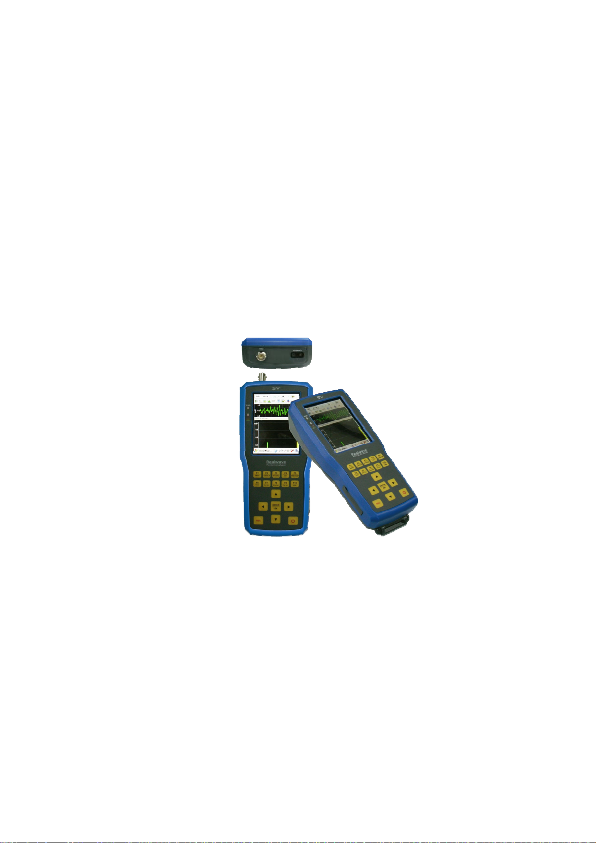
Smart Sound/Vibration Analyzer

(Real-Time Based Measurement System)

Manual

First Edition(Ver. 1.7)

SV Corp.

This document is on revising. We will upload the revised document to FTP Server(Refer next page)
at every revising. Of course, you can download a upgraded program(Smart Sound/Vibration
Analyzer.)

Copyright © by SV Corporation.

http://www.svdigital.com
ftp://realwave:[email protected]

email : [email protected]

, http://www.svemall.com

RM302, SangShin BD, 719-1, Yi-Dong, SangRok-Gu,
AnSan-City, KyongGi-Do, 426-857
South Korea
Tel. [phone]
Fax. [phone]

2

Contents

I. Composition of Smart Sound/Vibration Analyzer ............................................................................... 5

II. Installation & Operation Procedure ................................................................................................... 6

1. S/W Installation ............................................................................................................................ 6

2. H/W Installation .................................................... 오류! 책갈피가 정의되어 있지 않습니다.

3. Run and Registration .................................................................................................................... 7

4. Firmware Upgrade ....................................................................................................................... 8

III. Basic Functions of Program ........................................................................................................... 10

1. Icons ........................................................................................................................................... 10

2. Control of Wave File .................................................................................................................. 12

3. Open & save configuration. ....................................................................................................... 14

4. Data Export ................................................................................................................................ 14

5. Transducer type and Calibration ................................................................................................ 16

6. Recording Options ..................................................................................................................... 18

7. Recording Information ............................................................................................................... 19

IV. Real Time Measurement in Vibration Level Meter/Sound Level Meter ......................................... 21

1. Basic Theory of Vibration Level Meter / Sound Level Meter .................................................... 21

2. Setting of measuring option ....................................................................................................... 26

3. Display Option ........................................................................................................................... 32

4. Measurement and Storage .......................................................................................................... 33

5. Playback and Analysis ............................................................................................................... 34

6. Input of Measurement Information ............................................................................................ 35

7. Octave Analysis in Vibration Level Meter ................................................................................. 35

8. Setting options for Human Vibration Measurement .................................................................. 36

V. Real Time FFT SpectrumxSpectrogram and Octave Analysis .......................................................... 39

1. Understanding of Frequency Analysis ....................................................................................... 39

2. Fast Fourier Transform ............................................................................................................... 39

3. FFT Based Octave Analysis ....................................................................................................... 45

4. Weighting ................................................................................................................................... 46

5. Integration in Frequency Domain .............................................................................................. 48

6. Setting the Options of Measurement .......................................................................................... 49

7. Setting the option of display ...................................................................................................... 50

8. Record and Playback .................................................................................................................. 51

9. Mode Conversion of FFT Analysis, Spectrogram and Octave Analysis .................................... 51

VI. FFT Based RPM Meter .................................................................................................................. 52

1. Understanding about the RPM Measurement ............................................................................ 52

2. Frequency Analysis .................................................................................................................... 52

3

3. Measuring with RPM Meter ...................................................................................................... 53

VII. The way to use RealWave Desk for PC ........................................................................................ 55

1. Create a Project / Open .................................................................................................. 55

2. Adding a file / Delete ............................................................................................................. 56

3. Control of Graph ........................................................................................................................ 57

4. The Control of Property list ....................................................................................................... 57

5. Control of Sound ........................................................................................................................ 58

6. List of Result Report ............................................................................................................ 58

VIII. Installation of ActiveSync and Communication with PDA ......................................................... 60

1. What is Microsoft ActiveSync? ................................................................................................. 60

2. Installation of ActiveSync .......................................................................................................... 60

IX. The Usage of PDA ..................................................... 오류! 책갈피가 정의되어 있지 않습니다.

1. Start and End of the System .................................. 오류! 책갈피가 정의되어 있지 않습니다.

2. Start and End of Program ...................................... 오류! 책갈피가 정의되어 있지 않습니다.

3. Conversion of Application Program ...................... 오류! 책갈피가 정의되어 있지 않습니다.

4. Power Setting of PDA ........................................... 오류! 책갈피가 정의되어 있지 않습니다.

5. memory ................................................................. 오류! 책갈피가 정의되어 있지 않습니다.

6. Backlight ............................................................... 오류! 책갈피가 정의되어 있지 않습니다.

7. Deleting Programs ................................................. 오류! 책갈피가 정의되어 있지 않습니다.

[Appendix 1] ......................................................................................................................................... 64

The Theory for calculating RMS by ISO2631 and ISO8041 ............................................................... 64

[Appendix 2] ......................................................................................................................................... 67

Frequency Response of Filter in the Vibration Level Meter ................................................................. 67

1. 1Hz Highpass Filter ................................................................................................................... 68

2. 5Hz Highpass Filter ................................................................................................................... 69

3. 10Hz Highpass Filter ................................................................................................................. 70

4. 2Hz~300Hz Bandpass Filter ...................................................................................................... 71

5. 2Hz~1kHz Bandpass Filter ........................................................................................................ 72

6. 10Hz~500Hz Bandpass Filter .................................................................................................... 73

7. 10Hz~1kHz Bandpass Filter ...................................................................................................... 74

[Appendix 3] ......................................................................................................................................... 75

Theory of WBCombined Filter and Frequency Response .................................................................... 75

1. Theory ........................................................................................................................................ 76

2. Frequency Response and weight factor of Weighting Filter as acceleration input .................... 83

3. Frequency Response and weight factor of Weighting Filter as velocity input ........................... 86

4

I. Composition of Smart Sound/Vibration Analyzer

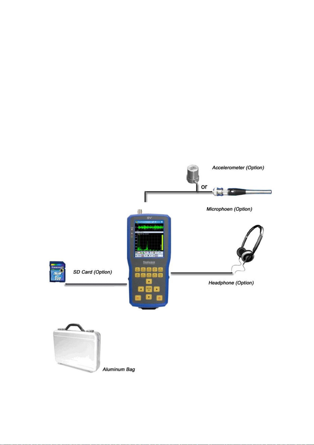
- AC Adapter: 1set

- USB Interface Cable: 1 ea

- Smart Sound/Vibration Analyzer: 1 ea

- S/W CD(RealWave S/W, Firmware Update S/W, RealWave Desk S/W) : 1ea

- Manual: 1 ea

- Portable Aluminum Hardcase : 1 ea

[Fig. I-1] System Diagram

5

II. Installation & Operation Procedure

1. S/W Installation

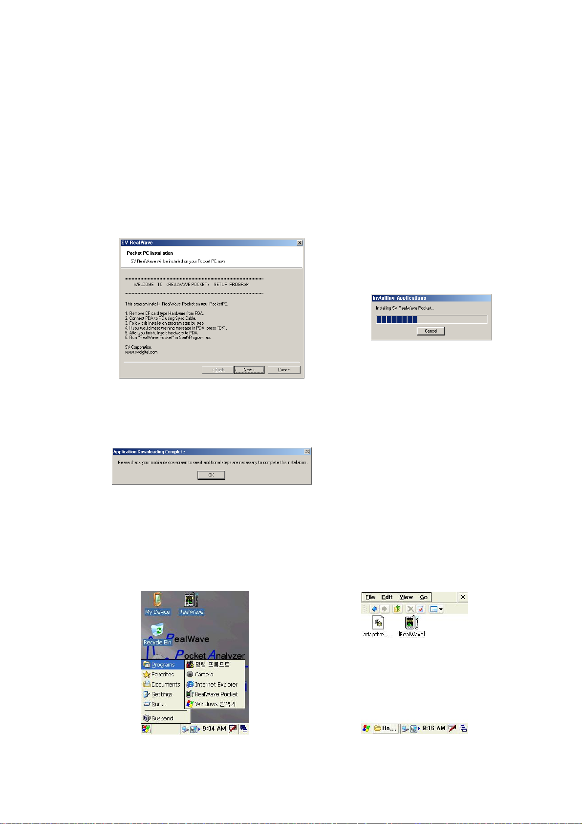
Before installing of the RealWave program on PDA, you must install ActiveSync on your PC.
Please refer to the chapter VIII to install ActiveSync. After installation of ActiveSync, connect PC
with PDA via USB cable and Insert the CD. Run the RealWave.exe file from the RealWave folder of
the CD-Rom drive. When the window appears like [Fig. II-1-1] and click ‘Next’, it can be proceed to
[Fig. II-1-2] and [Fig. II-1-3]. And then click ‘OK’ to finish installation [Fig. II-1-3].

Realwave.ARM.CAB files use when installing a program from PDA directly.

[Fig. II-1-1] Installation window 1

[Fig. II-1-3] Installation window 3

[Fig. II-1-2] Installation window 2

[Fig. II-1-4] Run of RealWave program 1

[Fig. II-1-5] Execute RealWave program 2

6

To run Launch RealWave program, click the tap [Start >> Programs], and then click ‘RealWave”
icon on the window of [Fig. II-1-5].

2. Run and Registration

2. 1 Unregistered PDA

If running RealWave program at unregistered PDA, please enter given license number on the
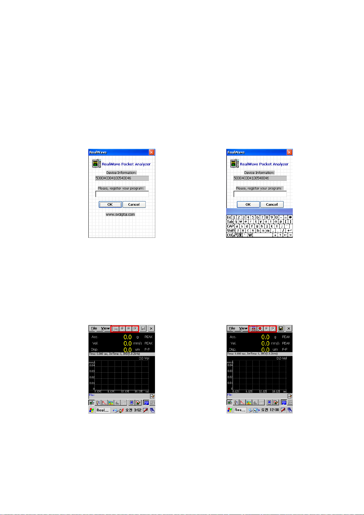
register window when appears a window like [Fig. II-2-1,2]. The license number is limited at only
one PDA. Once registered, RealWave program doesn’t work properly if the license number is
different. Please contact us when you have a problem with the license number.

[Fig. II-2-1] Registration window

2. 2 Pre-registered PDA

If you have PDA included package, program will start without register procedure like [Fig. II-2-1].
In case of no H/W or failure to recognize, icons in the red box are not activated like [Fig. II-2-3]. But
in case of the opposite, icons are activated and ready to measure like [Fig. II-2-4].

[Fig. II-2-2] Entering license number

[Fig. II-2-3] Failure to recognize H/W

[Fig. II-2-4] Properly recognized H/W

7

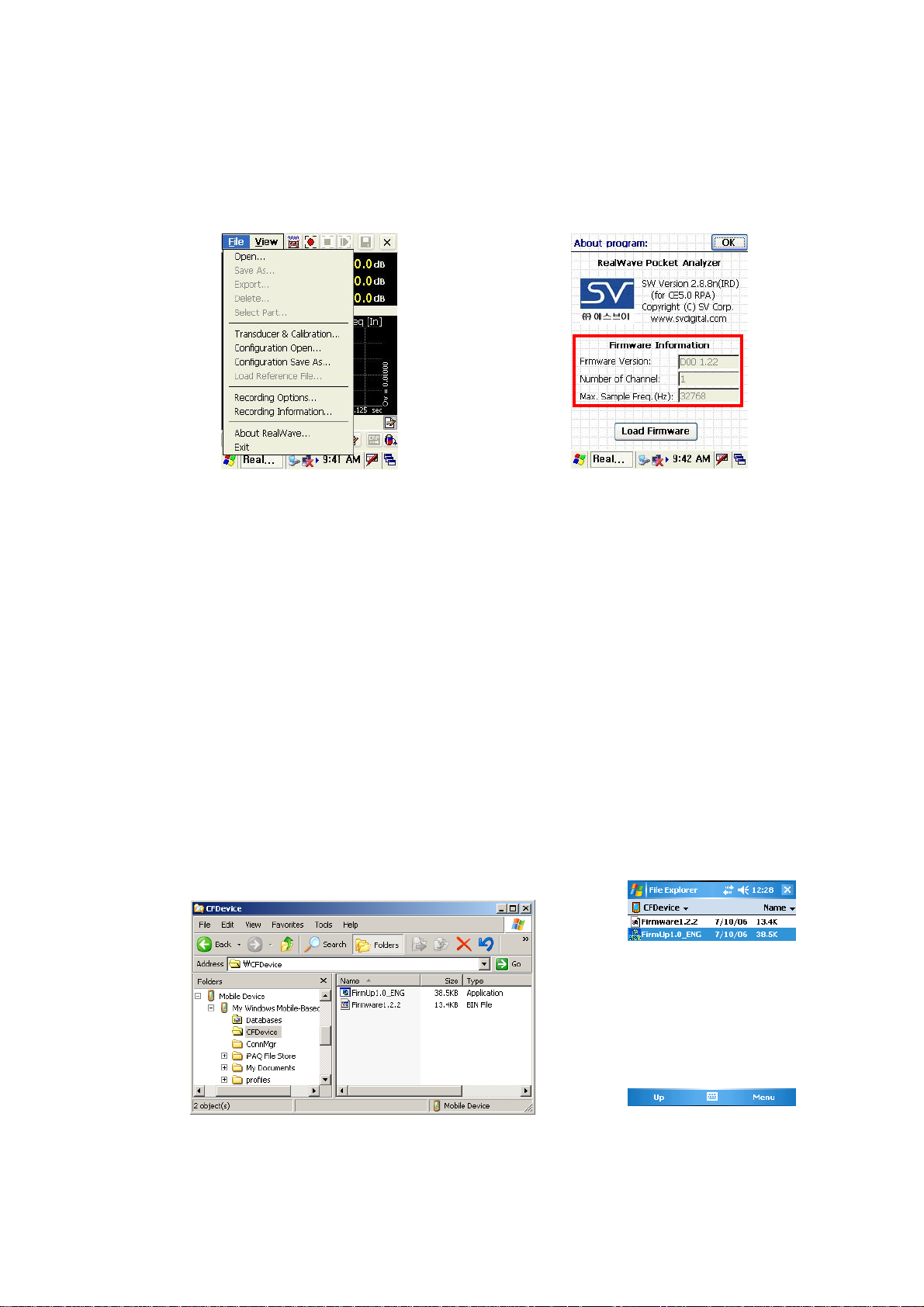
3. Firmware Upgrade

3. 1 Check firmware version

If you select [About RealWave] menu in [File], dialog window appears in [Fig. II-3-2]. You can
check the information of hardware including firmware version.

[Fig. II-3-1] Select [About RealWave…]

menu

3. 2 Firmware Upgrade

Smart Sound/Vibration Analyzer H/W has firmware inside, so the firmware has to be upgraded
when the new version is released. First, ‘FirmUp1.0_ENG.exe’ file in the RealWave software CD has
to be copied at a proper folder in PDA. Here is the way to copy it:

1) Copy the ‘FirmUp1.0_ENG.exe’ in the RealWave software CD.

2) Connect PDA with PC using a USB cable.

3) After ActiveSync connected, double click the ‘Mobile Devices’ folder on the windows explorer.
Several folder in PDA will be found.

4) Paste ‘FirmUp1.0_ENG.exe’ to the proper PDA folder.

[Fig. II-3-3] ~[Fig. II-3-4] shows a copy of ‘FirmUp1.0_ENG.exe’ file.

[Fig. II-3-2] Check firmware version

[Fig. II-3-3] Copy and Paste in the Window Explore

[Fig. II-3-4] Run ‘FirmUp.exe’

file on PDA

8

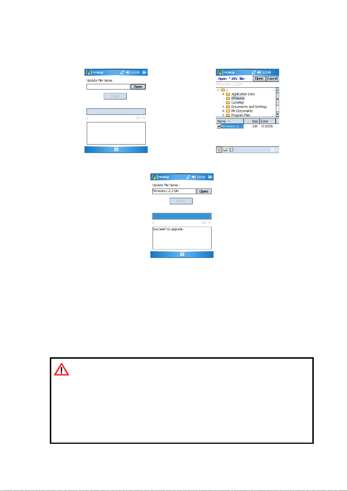
When running ‘FirmUp1.0_ENG.exe’ file on PDA, the program runs like [Fig. II-3-5]. Press
[Open] button on the window of [Fig. II-3-6]. Select folder and file (*.bin) to update and press [Open]
button on the window of [Fig. II-3-7].

[Fig. II-3-5] FirmUp window

[Fig. II-3-7] Completion to open a file to update

At [Fig. II-3-7], press [Start] button to start update. You must insert front-end H/W before update. It
is highly recommended to use AC adaptor or USB cable, but not to use PDA while updating. It is very
harmful that H/W is removed from CF card slot or shut down compulsorily while updating. If it

[Fig. II-3-6] Open a file to update

causes, you can’t to update it and the hardware has to be repaired.

You must turn off PDA after finishing upgrade(Or remove hardware from PDA and then insert
hardware again).

Attention before updating firmware!

1. Use of AC adaptor or USB cable is highly recommended.

 It is very harmful to use PDA while updating.
 If the firmware upgrade is failed, the hardware can’t be used anymore and must

be repaired.

Attention after updating firmware!

1. Turn off the power of PDA, and then Turn on.

9

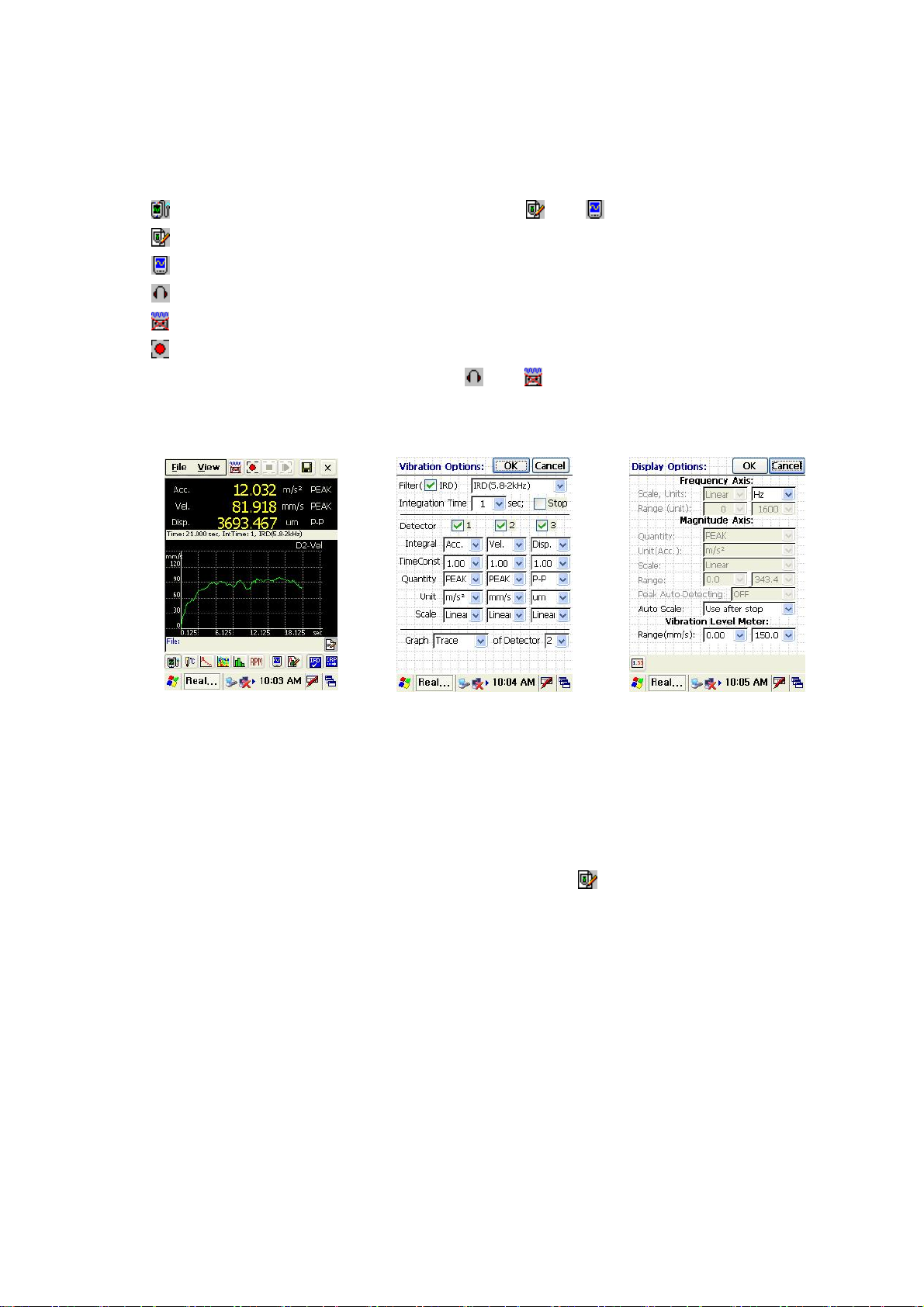
III. Basic Functions of Program

1. Icons

1. 1 Vibration Level Meter

Icon for vibration level meter mode [Fig. III-1-1]. and icons are activated.
Icon to set measurement option of vibration level meter mode[Fig. III-1-2]
Icon to control the result display[Fig. III-1-3]

Icon to hear sounds in real-time
Icon to display data only (without saving) in real-time and be called ‘ARM button’
Icon to measure and record wave file in real-time.

To accomplish sound hearing function, press

time

[Fig. III-1-1]

Vibration Level Meter

1. 2 Sound Level Meter

Upon clicking [File>> Transducer Calibration…] tap, [Fig. III-1-4] will appear, and if you choose

Vibration Options

and icons so that you can hear sounds in real-

[Fig. III-1-2]

[Fig. III-1-3]

Display Options

Microphone in Type option then you can use sound level meter.

Function of buttens are similar to Vibration Level Meter, icon

of sound level meter ([Fig. III-1-6]).

will appears measurement option

10

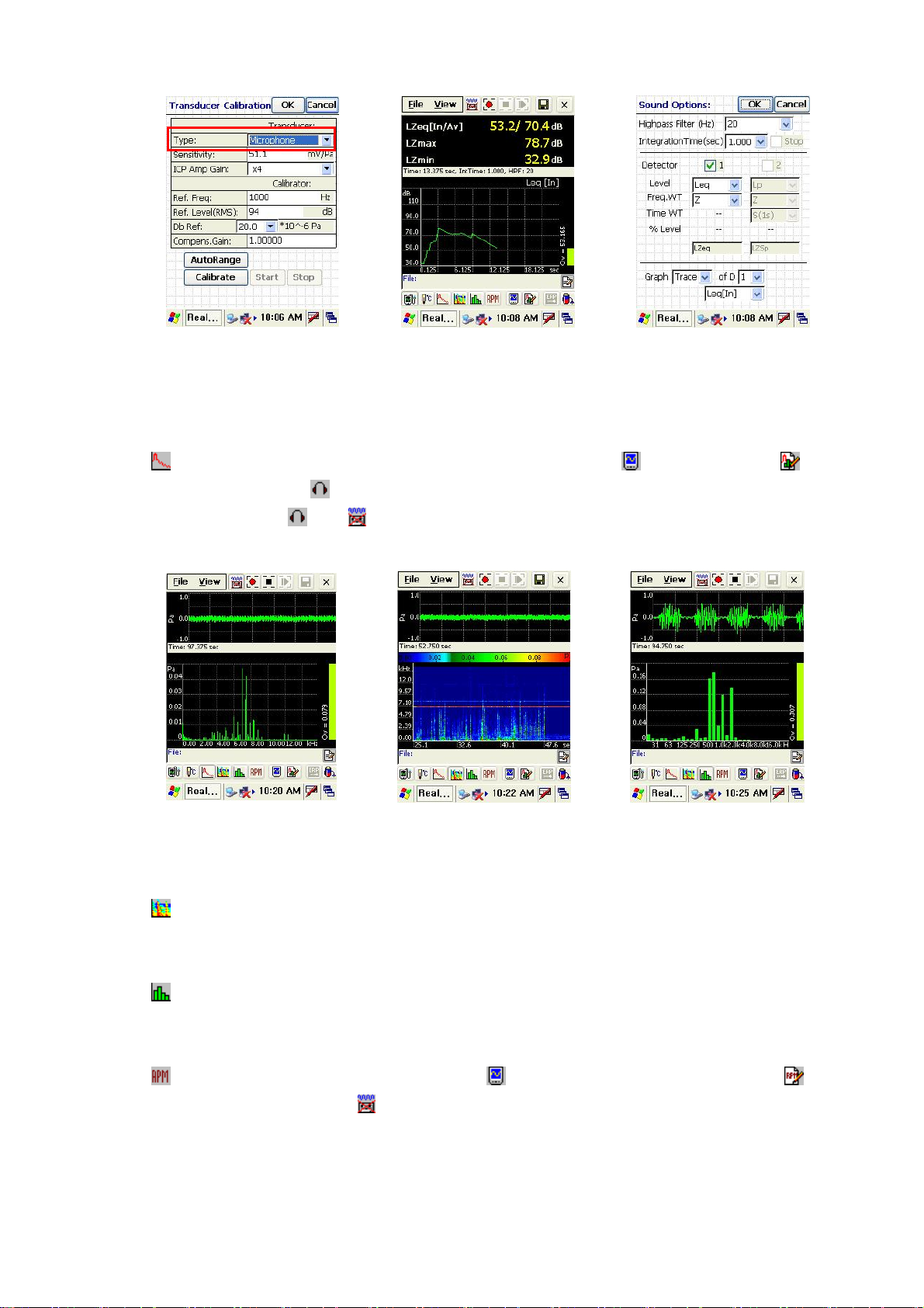
[Fig. III-1-4] Setting the Sound

Level Meter Mode

1. 3 FFT Analyzer

Icon for FFT Analyzer. If pressing the icon, graph control icon , option setting icon and

sound hearing mode icon
and microphone with

are activated. Likewise, you can also hear the sounds of accelerometer

and icons.

[Fig. III-1-5] Sound Level

Meter

[Fig. III-1-6] Sound Options

[Fig. III-1-7] FFT Analyzer

1. 4 Spectrogram

Icon for spectrogram. The activated icons are identical with FFT Analyzer.

1. 5 Octave Analyzer

Icon for FFT Based Octave Analysis. The activated icons are identical with FFT Analyzer.

1. 6 FFT Based RPM Meter

Icon to measure RPM. Graph control icon and measurement option control icon are

activated only. And Arm button

[Fig. III-1-8]Spectrogram

is only activated because it doesn’t support data store function.

[Fig. III-1-9] Octave Analyzer

11

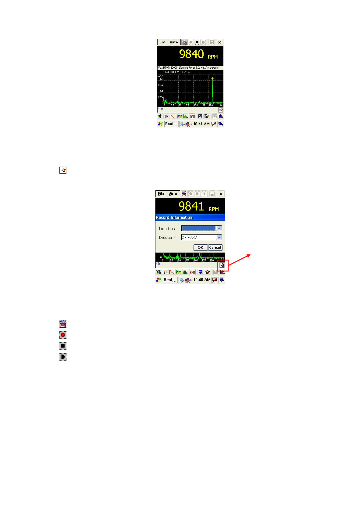
[Fig. III-1-10] RPM Meter

1. 7 Entering record information

Icon to enter record information. Record information window appears like [Fig. III-1-13].

click

[Fig. III-1-11] Record information window

1. 8 Measurement and Playback

: ARM mode – Icon to display data only in real-time without data store.

: Record mode – Icon to store wave file and data in real-time.

: Stop mode– Icon to stop arm, record and playback.

: Playback mode – Icon to analyze data playing wave file. The measured data with this function

is the same as the one of record mode.

2. Control of Wave File

2. 1 Open a file

When clicking [File] menu on lower left side of the screen, wave file can be controlled with [Open],
[Save As…] and [Delete] tap at [Fig. III-2-1]. To open file, click [Open] tap and choose a folder and a
file on the window as you wish at [Fig. III-2-2].

12

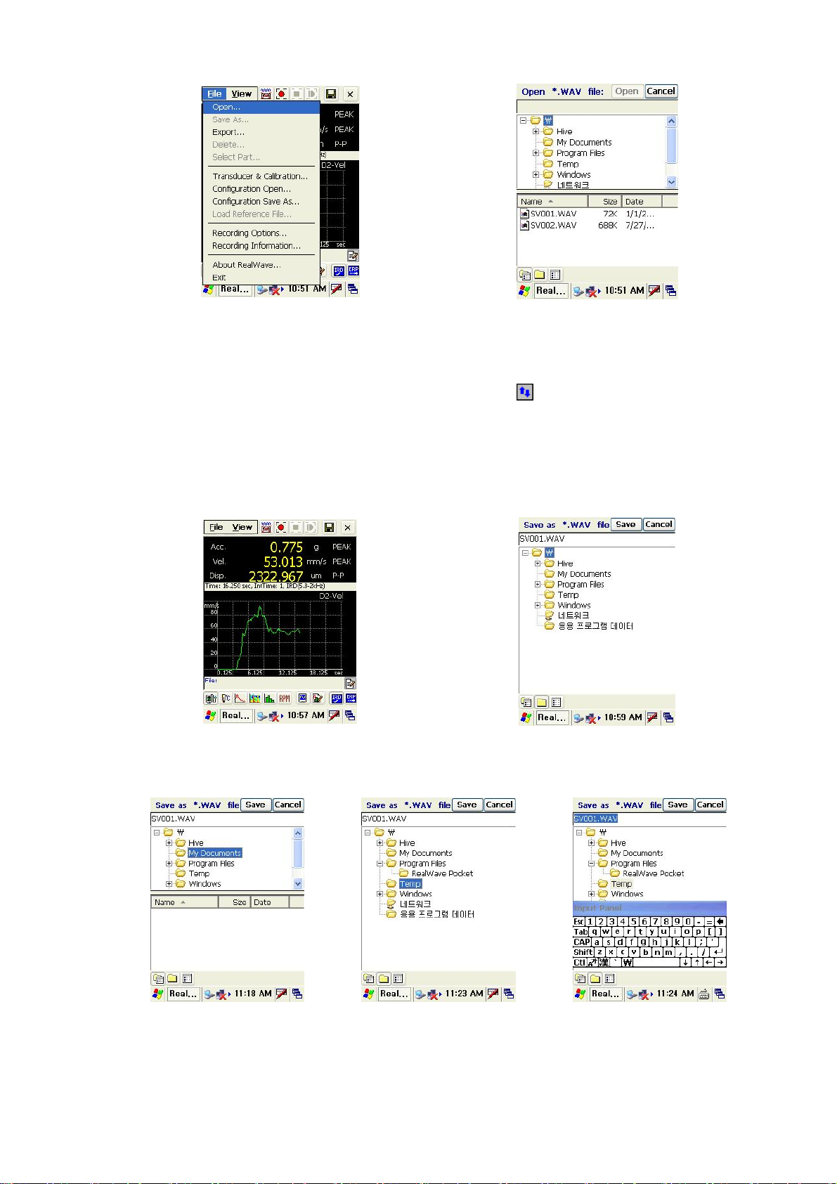
[Fig. III-2-1] Open a wave file

2. 2 Save As…

After opening a file, file name can be checked by clicking
III-2-3]. Upon clicking [File>>Save As…] tap, one of the window from[Fig. III-2-4] to [Fig. III-2-6]
will appear, so you can define a folder and file name at the window. [Fig. III-2-7] shows how to enter
a file name.

[Fig. III-2-2] Opening window of wave file

icon to convert window like [Fig.

[Fig. III-2-3] Confirmation of a file name

[Fig. III-2-5] Selection of a

folder and file to save as

another name

[Fig. III-2-6] Selection of a file

to save as another name

[Fig. III-2-4] Selection of a folder to save as

another name

[Fig. III-2-7] Entering a file

name

13

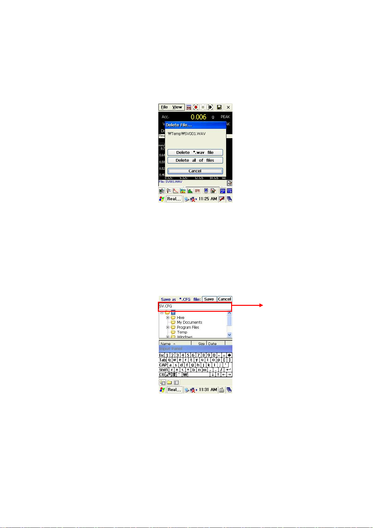
2. 3 Deleting currently opened file

[File>>Delete] is showed [Fig. III-2-8] and you can erase .wav file which are selected currently or
erase all files which include export files. It will not be activated if there’s no opened file. (When
selecting [File>>Delete] tap, currently opened files are deleted.)

[Fig. III-2-8] Deleting currently opened file

3. Open & save configuration.

[File>>Configuration Save As…] is to save all of currently configured options (measurement and
graphic display option) of the program. [File>>Configuration Open…] is to open and change to the
saved configuration. Extension of the saved file is *.CFG.
The functions of ‘Open’ and ‘Save As…’ is similar to that of chapter 2 “Control of Wave File”.

Entering file name

[Fig. III-3-1] Entering a configuration file name.

4. Data Export

4. 1 Vibration Level Meter Mode

Each different data is exported according to the display option. When displaying only vibration
value like [Fig. III-4-1], it doesn’t support to export data. On the other hand, when displaying
vibration value and trace like [Fig. III-4-2], it supports to save the changed values and export as an
image file.

14

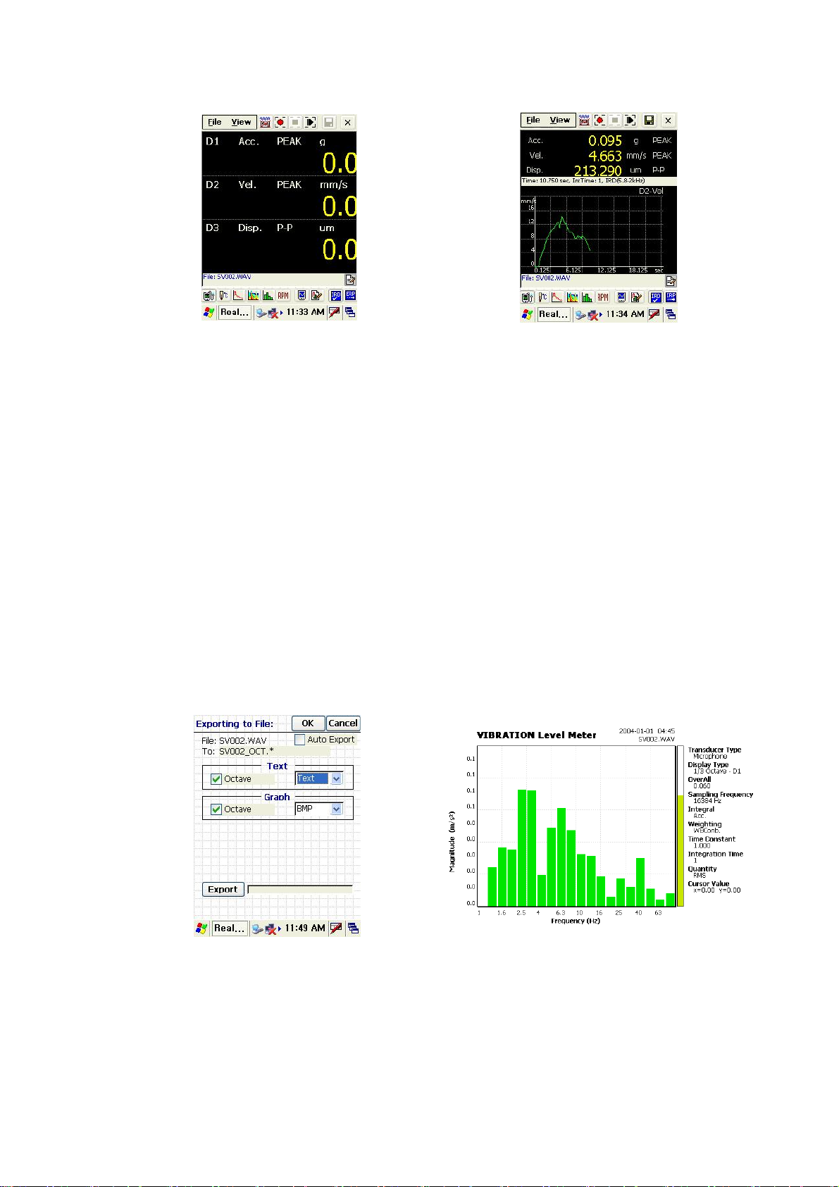
[Fig. III-4-1] Vibration value display

To export data, click [File>>Export] tap, and then the window [Fig. III-4-3] is opened. Check the
data or image file which wants to export, select file type and click ‘Export’ button. At last, just close
window by clicking [Ok] button.

 The supported data file type : Text, Excel, MATLAB

 The supported image file type : BMP, JPEG

[Fig. III-4-4] shows exported file and filename is similar to wave file’s name. For example,
exported octave image file is named as [wave file name_OCT.bmp].
If you should select [Automatic Export], dialog box shown in [Fig. III-4-6] would appear after every
measurement. Pressing [Export] button have data be exported automatically as option.

[Fig. III-4-2] Vibration value and Trace display

[Fig. III-4-3] Export window

[Fig. III-4-4] Exported octave image file

15

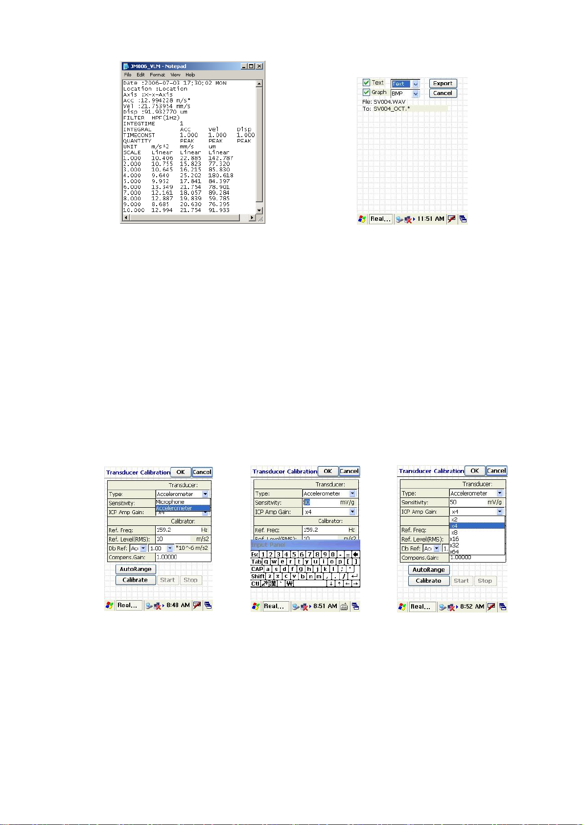
[Fig. III-4-5] Exported octave data file (TEXT)

4. 2 Sound Level Meter, FFT, Spectrogram, Octave Mode

Sound Level Meter, FFT and Octave analysis mode support both data and graph image export. But
spectrogram mode supports graph image export only. In the exported data, the frequency and
corresponding values are arranged vertically.

[Fig. III-4-6] Automatic Export After

measurement

5. Transducer type and Calibration

5. 1 Selection of transducer type and entering sensitivity

By clicking [File>>Transducer Calibration…] tap, [Fig. III-5-1] window is opened.

[Fig. III-5-1] Selecting

transducer

ICP(IEPE) type microphone and accelerometer is supported and input sensitivity data as shown on
[Fig. III-5-2].

5. 2 AutoRange and Gain adjustment

This system supports digital gain adjustment by 1, 2, 4, 8, 16, 32 and 64 times. It is preferable to

[Fig. III-5-2] Entering

sensitivity

[Fig. III-5-3] Gain adjustment

16

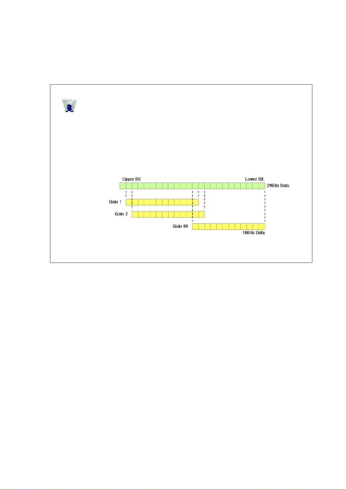
adjust gain if the signal is low. To use AutoRange function is more desirable than hand-operated
adjustment.

[AutoRange] calculates input signal and automatically adjusts gain. So it would be better to
accomplish AutoRange before calibration. [Fig. III-5-3] shows AutoRange process.

HighTech

1

RealWave H/W has an analog gain with 10 times, but digital gain is used at gain
adjustment. Analog amplifier accomplishes the role of Pre-Amplifier. Work of the
analog amplifier depends on the cable connected to the sensor.

Digital gain usually uses the method that multiplies an original signal by any gain,
but it also amplifies noise with signal. So this system doesn’t use the method.

This system uses the 24bits for ADC(Analog to Digital Convert) and 16bits data
is extracted from 24bits data. Therefore, the Digital Gain means to extract data
shifting bit position as figure below when extracting 16bits data from 24bits data.

Unlike conventional method using fixed magnification, It is very effective to
amplify signal without the amplification of noise.

5. 3 Calibration

After selecting type of transducer and entering sensitivity and adjust gain, click [Calibrate] button.
A graph window will appear like [Fig. III-5-5]. It is only the status to display data in real-time without
measurement. By clicking [Start] button, it is calibrated during 10 seconds. After calibration, [Fig. III­5-6] will appear and the result is calculated by compensated gain.

Generally, calibrated sensitivity can be calculated as follows:

Compensated Sensitivity = Compensated Gain × Inputted Sensitivity <Eq. III-5-1>

If it is calibrated inadequately, you can return to the pre-calibrate status by clicking [1.0] button. In
case calibrated gain value is smaller than 0.5 or exceeds 1.5, an alarm message will be pop up and the
transducer cable or the power of calibrator need to be checked.

17

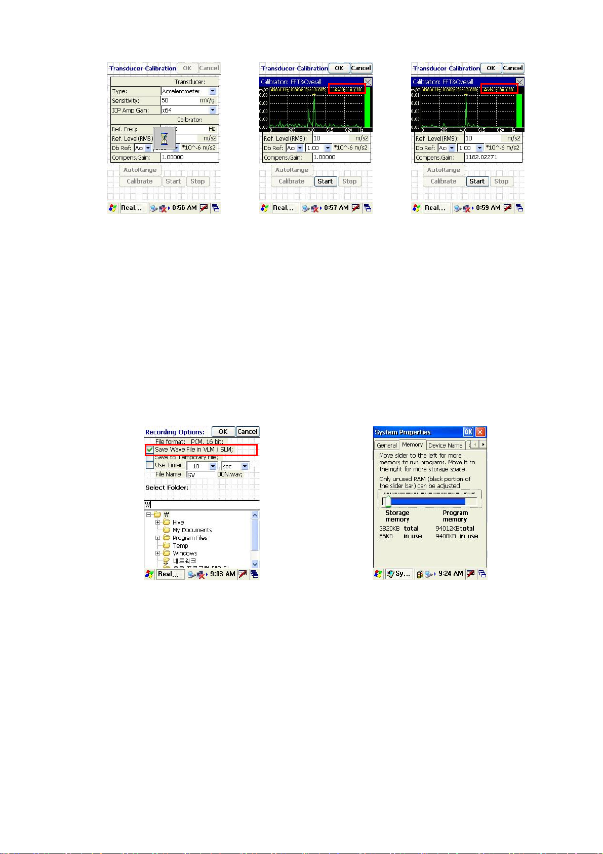
[Fig. III-5-4] AutoRange

[Fig. III-5-5] Calibration

window

[Fig. III-5-6] Completion of

calibration

6. Recording Options

When selecting [File>>Recording Options…] tap, a recording option window will appear like [Fig.
III-6-1]. [Save Wave File I n VLM / SLM] option is for if saving wave file in vibration level meter /
sound level meter mode or not. By checking the option, vibration values / sound values and wave
files are stored simultaneously. If it is not checked, actual wave data will not exist although file name
will remain.

[Fig. III-6-1] Recording options window

[Fig. III-6-3] shows the difference between checking [Save Wave File In VLM] option and no
checking the option on the vibration level meter mode. The size of ‘SV001.wav’ is only 44Bytes at
[Fig. III-6-3]. It means there’s no actual recorded data. On the contrary, ‘SV002.wav’ has 640kBytes.
It means that there’s actual data.

[Fig. III-6-2] Memory information window

18

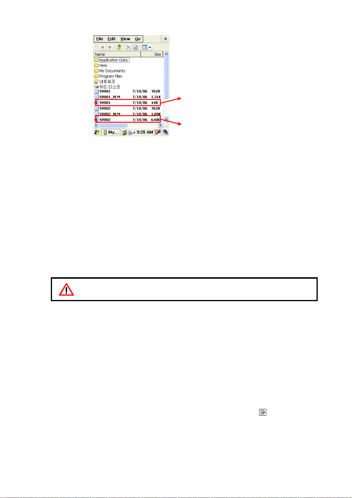
No real data but only wave file name
exists.

This wave file has the actual data.

[Fig. III-6-3] Saving wave file on vibration level meter mode

- [Use Timer] option is to define time duration. Measurement is accomplished during the defined
duration and stop automatically. For example, if the timer is set 10 sec., it will measure only for 10
seconds.

- [File Name] option is to define file name. Once measurement is accomplished, each recording
session automatically generates numeric name after the given file name. For example, let us consider
a series of measurements with the name “SV”, numeric name automatically generated as
“SV001.wav”, “SV002.wav”, etc.

- [Select Folder] option is to select folder to save files.

- [Memory Info…] button shows memory information like [Fig. III-6-2].

To prevent losing data in case of battery discharge, it is recommended to set
saving folder to the ‘SD Card’.

7. Recording Information

Recording Information window is for entering the recording information (Name, object or axis of
measurement etc.).

- [Name] : Operator

- [Object] : Object of measurement

- [Location] : Location of measurement

- [Direction] : Measurement directions of accelerometer as x, y, z-axis.

In [Location] option, you should enter the location information where measurement is
accomplished in advance, and then choose pre-defined location by clicking

icon. To add new
location information, it is easily added by clicking [add] button after entering new location
information . To delete it, select a list and click [Del] button. Do not use special character \ / : * ? “ < >
for [Location], after the measuring it will use for folder name in desk program,

19

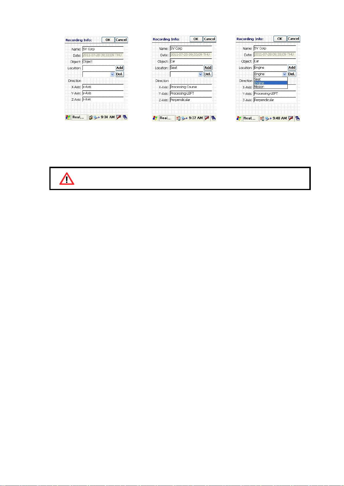
[Fig. III-7-1] Recording Info.

Do not use special character \ / : * ? “ < > for [Location]

[Fig. III-7-2] Completion to

enter Rec. Info.

[Fig. III-7-3] Example of pre-

defined location

20

−

τ

IV. Real Time Measurement in Vibration Level Meter/Sound Level Meter

1. Basic Theory of Vibration Level Meter / Sound Level Meter

1. 1 Understanding of Integration Time and Time Constant

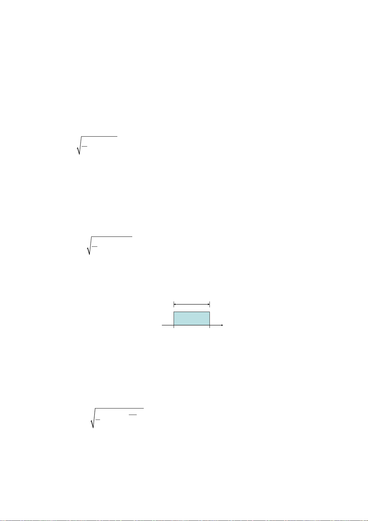
The RMS(Root-Mean-Square) calculation routine is based on “IEC60804:2000-Integrated
Averaging Sound Level Meter” and “ISO8041:1990-Human response to vibration-Measuring
instrumentation”.

Generally, RMS is calculated by the equation below :

T

1

aatdt

=

rms

2

∫

0

T

<Eq. IV-1-1>

()

where

()at is instantaneous acceleration and T is measuring time.

a is calculated for T

rms

second. The calculation method in real-time is named Running RMS Acceleration which is described
at ISO(International Standard Organization) standard.

The RMS calculation equation in real-time can be arranged as below :

t

1

0

at atdt

rms

=

() ()

0

T

∫

tT

0

2

−

<Eq. IV-1-2>

where

t is current time, T is measurement period(time) for calculation. Sometimes, this period

0

is called by integral time. This calculation for RMS is linear Averaging RMS.

T

t

tT

0

[Fig. IV-1-1] The Calculation Method with Linear Averaging RMS

t

0

The linear averaging RMS Method is used for RMS, but is inferior to the exponential averaging

RMS in real-time calculation. The equation below represents the exponential averaging RMS.

tt

−

t

1

o

() ()

at atedt

rms o

=

τ

,

τ

2

∫

−∞

o

τ

<Eq. IV-1-3>

where

is the time constant and we can read it with ‘tau’ pronunciation. As [Fig. IV-1-2] is
shown, the exponential averaging RMS equation is different to the linear averaging RMS, but the
results are similar and the former emphasizes recent data of signal as [Fig. IV-1-2].

21

τ

−

Generally, the time constant is set with 0.035sec(Impulse), 0.125sec(Fast), 1sec(Slow). Each term
of times writes in the parenthesis. If you want to measure the impulse signal, you have to use 0.035
sec time constant. If you use more time constant (more than 10sec), the RMS has crushed values and
the response time is also slow.

Linear Averaging

Exponential(τ=RC) Averaging

t

t

tT

0

Averaging Time

o

[Fig. IV-1-2] Running RMS Calculation with Exponential Averaging

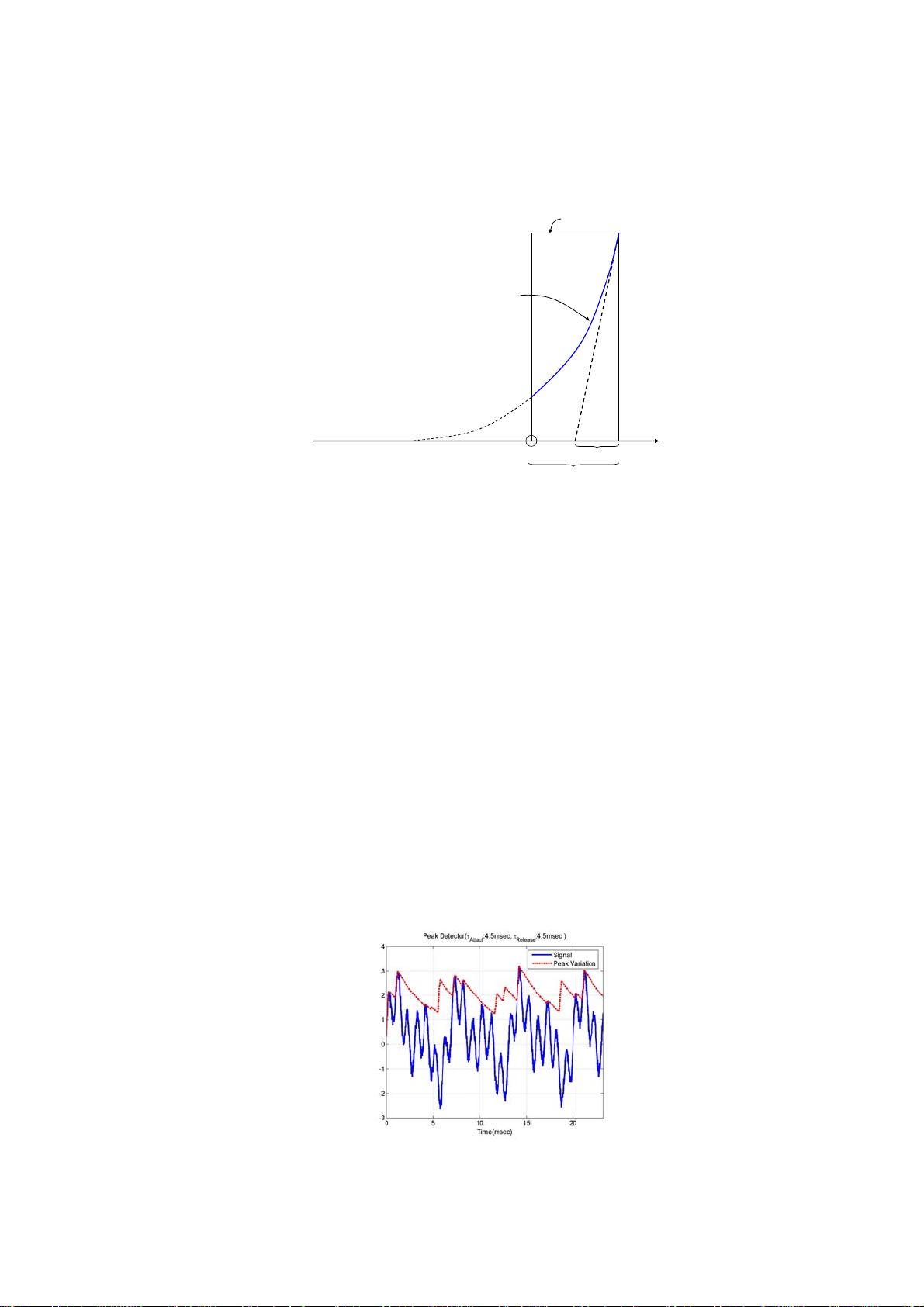
1. 2 Detector with Exponential Averaging Function

The full procedure of RMS(Root-Mean-Square) Detector is described in [1. 1] paragraph. When
peak values are calculated, we also use Peak Detector with exponential averaging. [Fig. IV-1-3]
shows how to detect peak values in real-time.

Peak Detector has two time constants. One is the attack time constant and another is the release (or
decay) time constant. The attack time constant means how peak values increase quickly. And the
release time constant means how the peak values decrease slowly after a peak.

Both time constants are defined from the user definable time constant in the program. If the release
time constant is smaller than 1.5sec, this is set by 1.5sec automatically which is defined in
“BS60651(IEC60651:1979) – Specification for Sound Level Meters”.

[Fig. VI-1-3] shows the variation of peak as the time signal in our system. This peak is calculated
from the absolute of time signal.

[Fig. IV-1-3] The Peak Variation of Time Signal

22

−

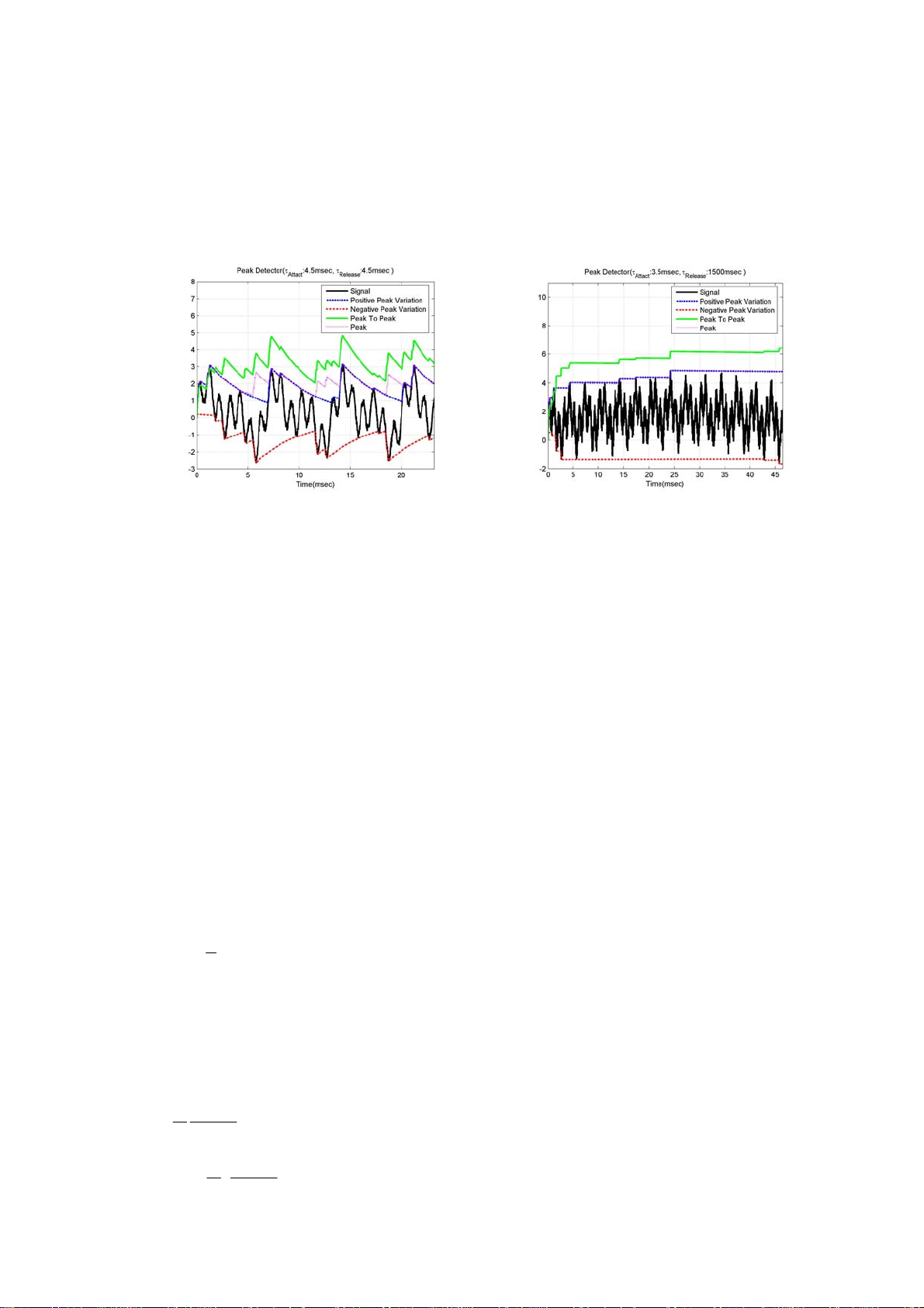
For getting the peak-to-peak(P2P) value, our system also use detector. At first, the positive and
negative peak values are calculated, and then we can get P2P from the difference of positive P2P and
negative P2P. The positive peak values are calculated from the positive signal and the negative peak
values are calculated from the negative signal. [Fig. IV-1-4] and [IV-1-5] shows how to calculate P2P
from signal.

[Fig. IV-1-4] A Case of Small Release Time

Constant

1. 3 Calculation of the Maximum of Signal (Max. Detector)

Peak Values are decreased with the release time constant as time goes. If you want to observe the
peak value(or maximum) during measuring, you have to use the maximum detector. You can’t
observe the peak value with peak detector. The value is found from the signal during the integration
time. For example, suppose that the integration time is 5sec. This system finds the maximum value
from time signal with 5sec and then saves and displays it to file at every 5sec. the integration time is
shown as

1. 4 Integrator

The theory of discrete integrator is classified into 3 types. There are Trapezoidal, Forward Euler
and Backward Euler. Integrator is written like below in the

T at [Fig. IV-1-1]

[Fig. IV-1-5] A Case of Big Release Time

Constant

s domain

:

Hss=

After this equation is rearranged with the bilinear Z Transform method, the integrator is written as
below in the

=

s

Hz

1

()

Tz

()

<Eq. IV-1-4>

21

−

z

−

−

1

+

Tz

=⋅

21

zdomain−

1

<Eq. IV-1-5>

1

−

1

+

−

−

z

:

1

<Eq. IV-1-6>

1

23

s

s

1

where

TF=

,

F is Sampling Frequency. RealWave uses the “Forward Euler” method, which is

simplified from Trapezoidal Method. We can write it as below :

1

−

Hz

()

Tz

=

1

<Eq. IV-1-7>

1

−

z

−

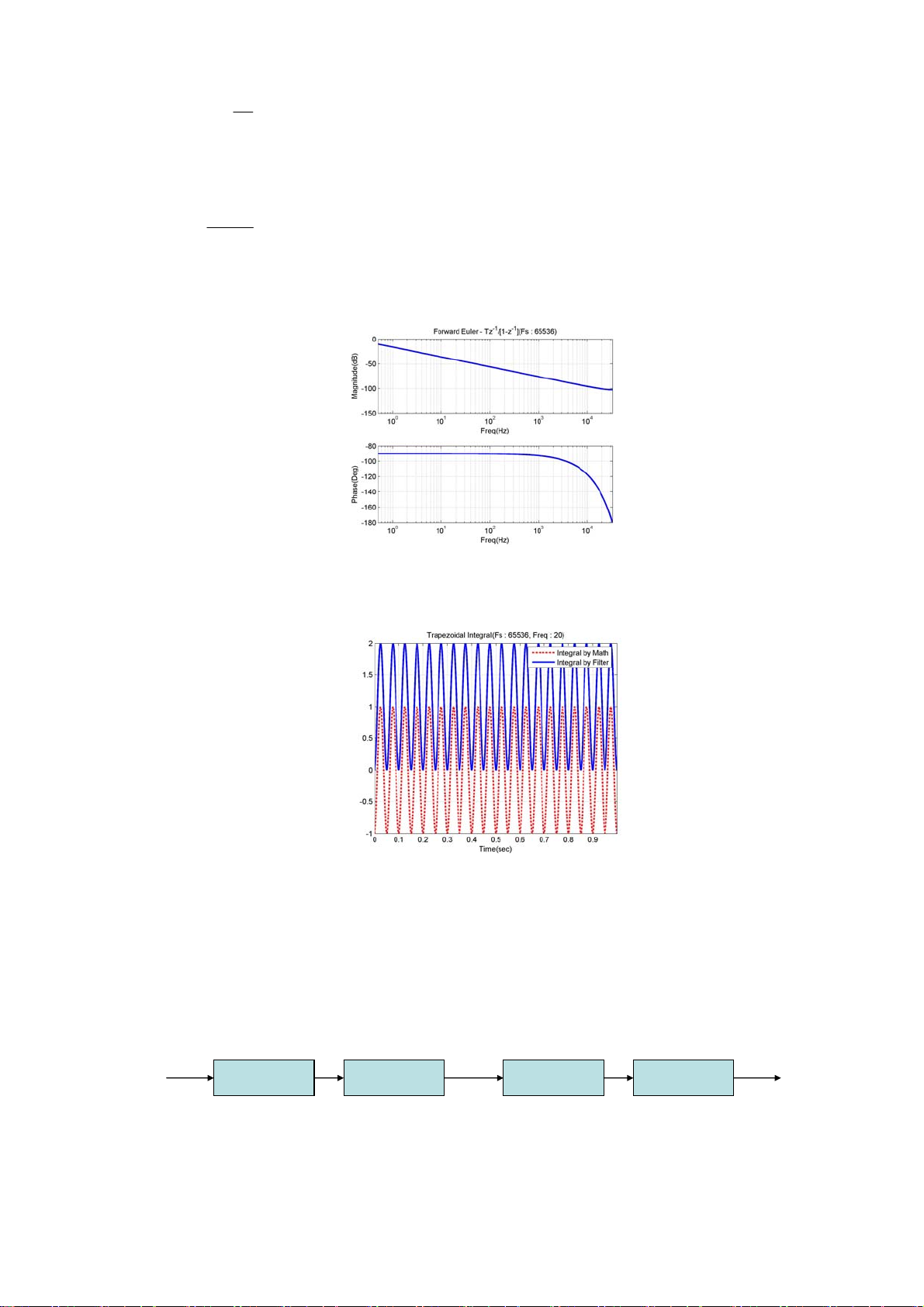
The frequency response function of integrator is shown in the [Fig. IV-1-6].

[Fig. IV-1-6] Frequency Response of Forward Euler Integrator

[Fig. IV-1-7] Integrated Result

Discrete integrator generates offset of signal (see [Fig. IV-1-7]). We must use highpass filter for
removing the offset. The highpass filter with 10Hz cutoff frequency (2-pole Butterworth IIR Filter) is
used in RealWave. The procedure for velocity and displacement is shown in the [Fig. IV-1-8]

Acceleration

Integrator

Highpass filter

(10Hz)

Velocity

Integrator

Highpass filter

(10Hz)

Displacement

[Fig. IV-1-8] Flow-chart for integration

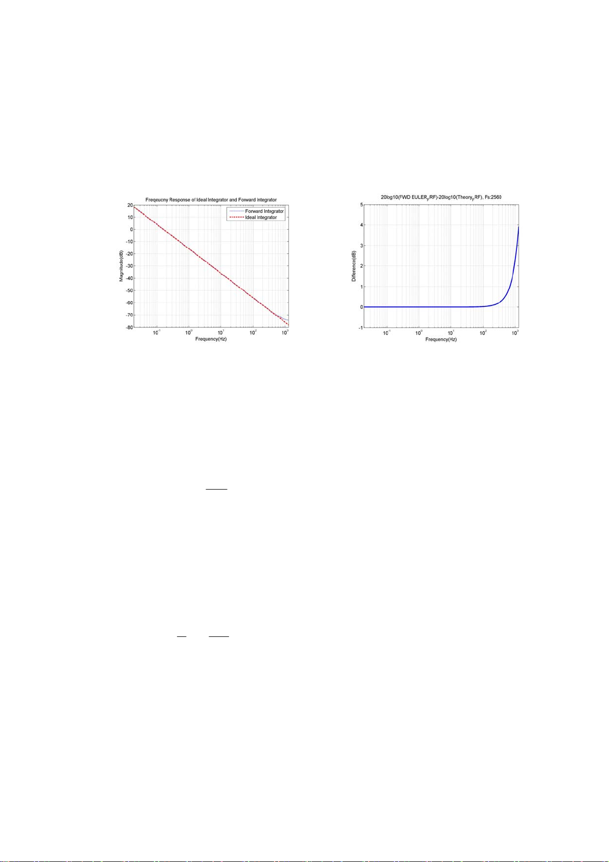
Discrete integrator has original error as shown in the [Fig. IV-1-9 ]. Specially, that error increas es

24

p

′

p

p

p

p

′

p

gradually in the high frequency region. But the integrated values(velocity or displacement) have a
very small values less than -50dB. Finally, the errors rarely affect the integrated value.

The integrated values have linearity in the low frequency which is in range of 23% of sampling
frequency. If a sampling frequency is set 10 times of the wanted frequency, we can get a good
linearity in the wanted frequency. Therefore, the sampling frequency is set 1024Hz because the useful
frequency range in the human vibration level meter is 80Hz.

[Fig. IV-1-9] Frequency Response

[Fig. IV-1-10] Phase Resp onse

1. 5 Sound Pressure Level Calculation

Differently with Vibration Level Meter, you can calculate dB value of measured sound signal
which uses microphone using such below basic theory through the chapter1.1 to 1.4.

Sound Pressure Level (SPL) is composed as below.

⎛⎞

′

p

SPL L

=⋅

()20log

P

rms

ref

Equivalent continuous Sound Pressure Level (

⎛⎞

1

L

eq

10 log

=⋅

⎜⎟

10

⎜⎟

Tp

⎝⎠

rms

⎜⎟

10

⎜⎟
⎝⎠

p

ref

: Root Mean Square (Pa)

: Reference Sound Level (20 Paμ)

L ) is expressed as below.

eq

⎛⎞
⎜⎟

∑

⎜⎟
⎝⎠

2

′

p

ref

′

: Real Sound Pressure (Pa)

You can get Equivalent continuous A-weighted sound pressure level when A-weighted
replaces

: Reference Sound Level (20 Paμ)

ref

T : Measurement Time

′

from this equation.

A

25

2. Setting of measuring option

2. 1 Selection of Filter

2. 1. 1 Filter selection of vibration level meter

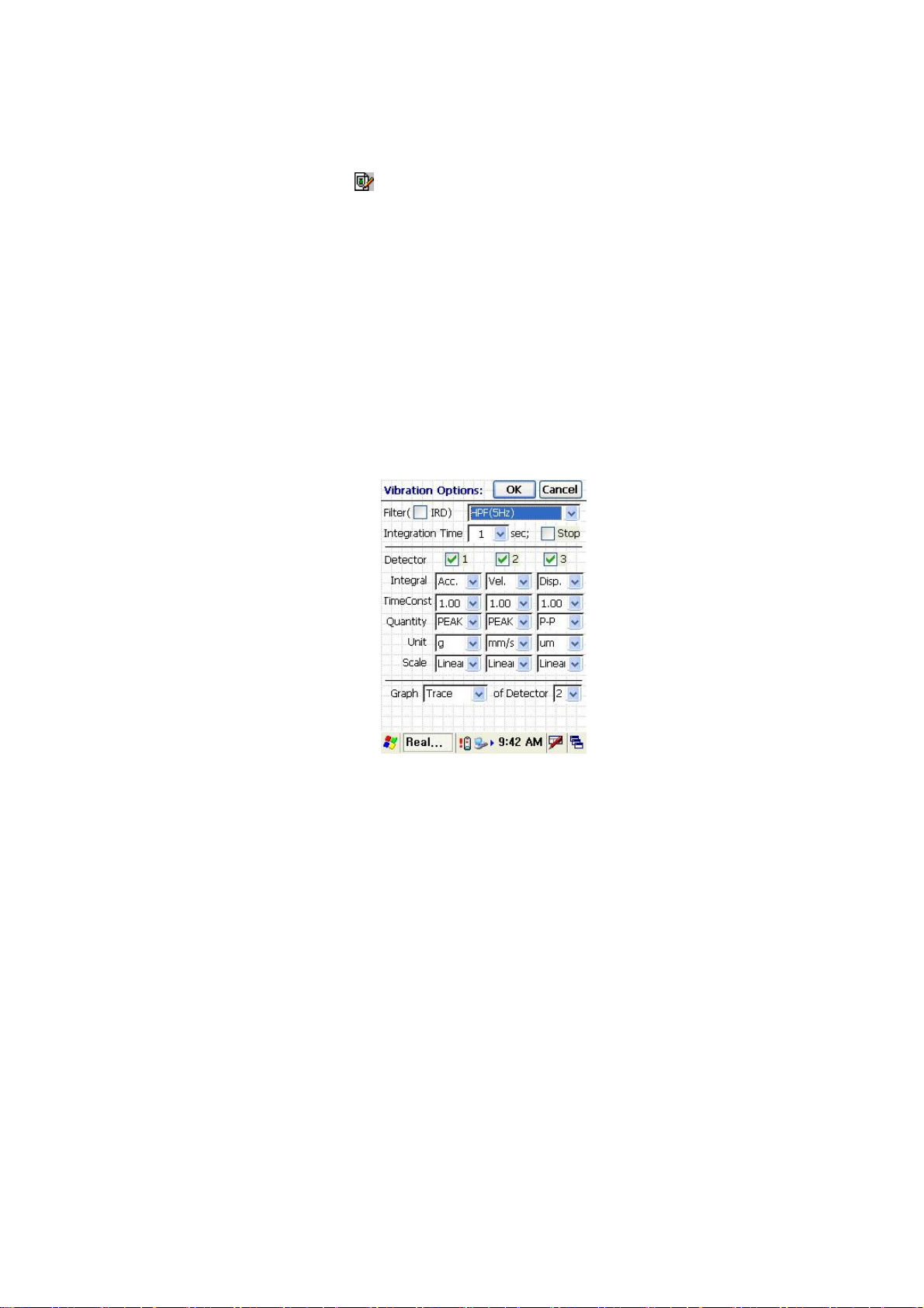
A window is opened to press

Here are the list below :

- 1Hz Highpass Filter

- 5Hz Highpass Filter

- 10Hz Highpass Filter

- 1KHz Highpass Filter

- 2Hz ~ 300Hz Bandpass Filter

- 2Hz ~ 1kHz Bandpass Filter

- 10Hz ~ 500Hz Bandpass Filter

- 10Hz ~ 1kHz Bandpass Filter

- WBCombined Filter (ISO6954)

button like [Fig. IV-2-1]. You can see 9 type filters.

[Fig. IV-2-1] Parameter Selection Window in Vi bration Level Meter

And another option is supplied for low frequency analysis as below :

- BW 1.6kHz : it means 1.6kHz bandwidth for analysis, Sampling Frequency is 4096Hz.

- BW 200Hz : it means 200Hz bandwidth for analysis, Sampling Frequency is 512Hz.

- BW 100Hz : it means 100Hz bandwidth for analysis, Sampling Frequency is 256Hz.

Highpass Filter uses 2-pole Butterworth Filter, Bandpass filter uses 4-pole Butterworth Filter. And
Whole-Body Combined filter is made with being based on the ISO6954 and ISO8041.

The frequency response of the each filter is shown in the [Appendix 2 : The frequency response of
Vibration Level meter] and [Appendix 3 : The frequency response of whole-body vibration filter].
And if you select WBCombined filter, Quantity value become initialize to RMS value.

26

If you select WBCombined filter, Quantity value become initialize to RMS value.

2. 1. 2 Filter selection of sound level meter

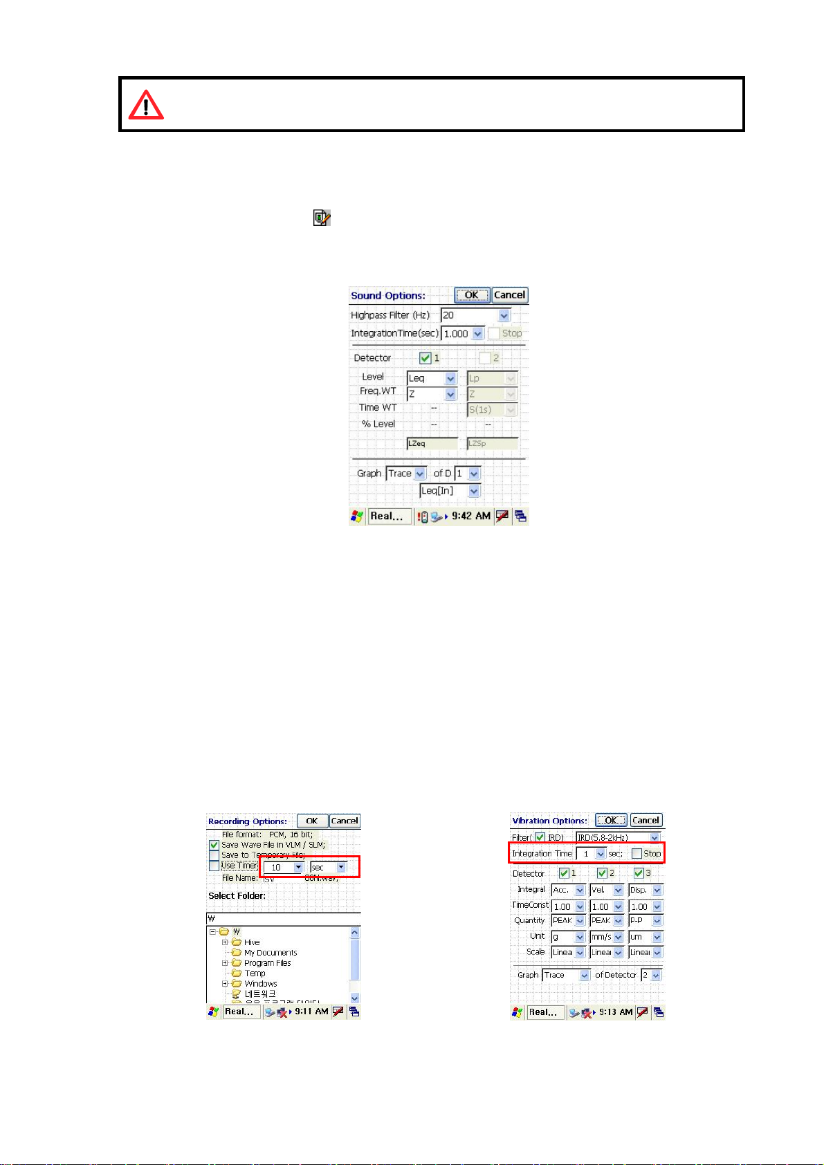
A window is opened to press

- 1Hz Highpass Filter

- 20Hz Highpass Filter

[Fig. IV-2-2] Parameter Selection Window in Sound Level Meter

2. 2 Integration Time

This parameter is the

T of <Eq. IV-1-1> and <Eq. IV-1-2> and means the measuring time or the

button like [Fig. IV-2-2]. You can see 2 type filters.

observation time. The calculated values are saved to file at every integration time. If you select stop
check box in [Fig. IV-2-4] and [Fig. IV-2-5], RealWave will stop measuring in the integration time.
Also if you select [Timer] in the [Recording Options] and [Stop] in the integration time
simultaneously, the system will stop at a short time. For example, if the timer is set by 10sec and the
integration time is set 2sec without stopping function, the system will save the 5 data at every 2sec
and stop after 10sec.

[Fig. IV-2-3] Timer Setting

[Fig. IV-2-4] VLM Integration Time Setting

27

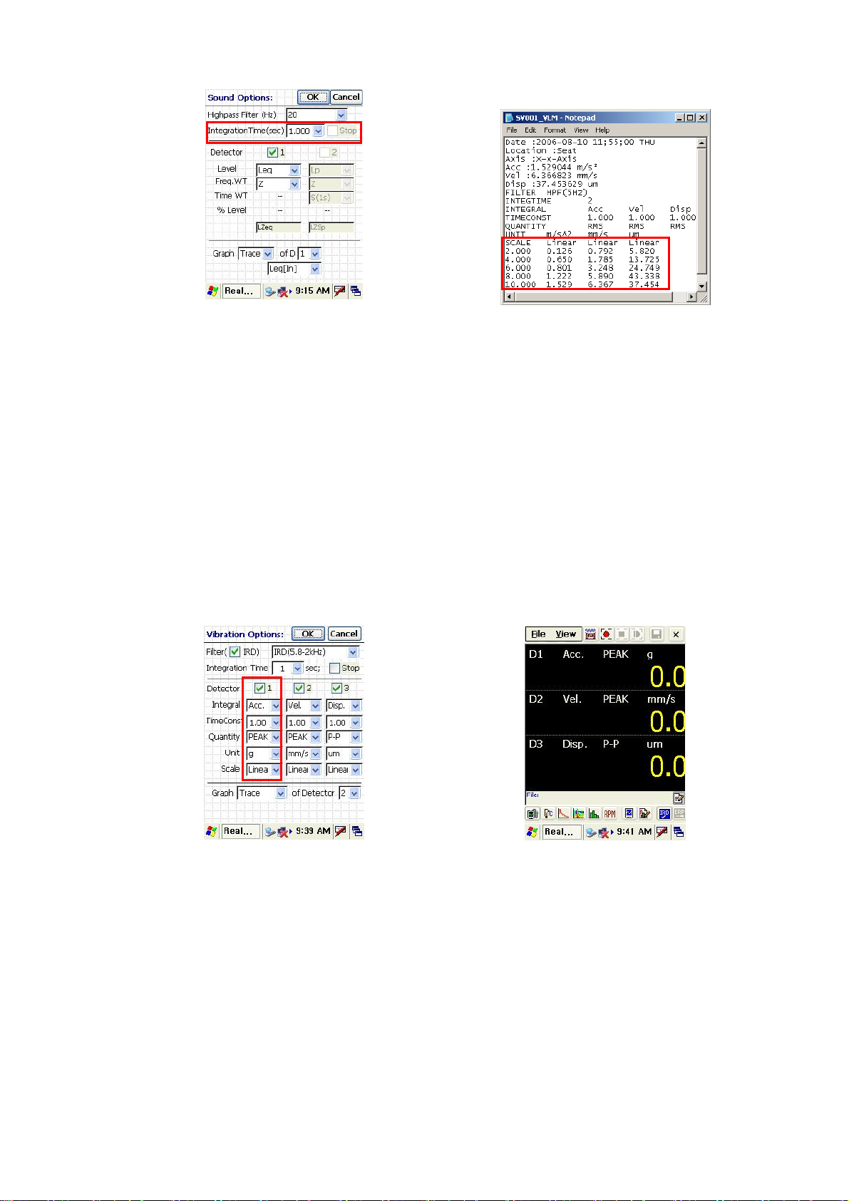
[Fig. IV-2-4] SLM Integration Time Setting

2. 3 Detector

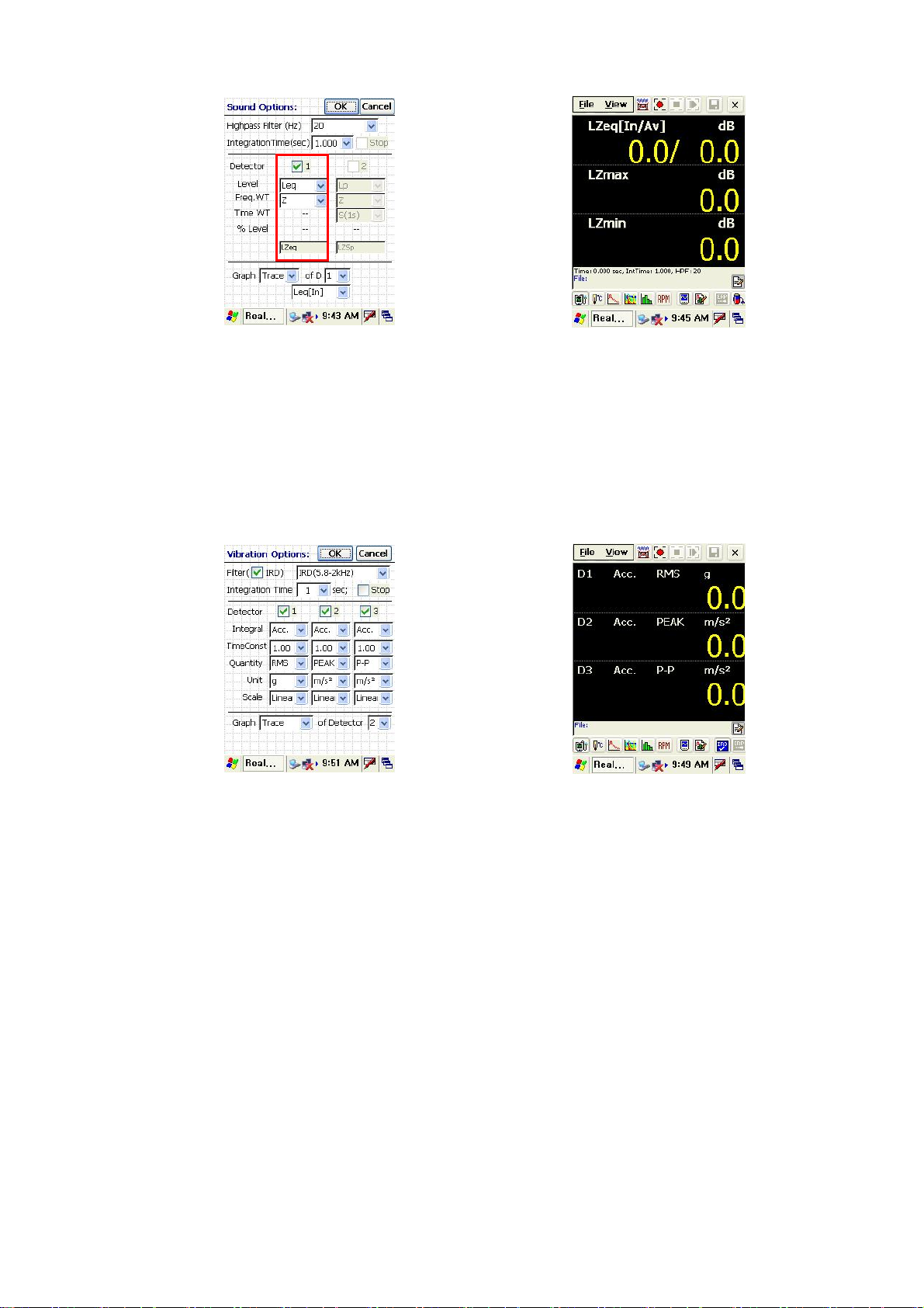
The results of 3 detectors are displayed in vibration level meter and 2 detectors are displayed in
sound level meter simultaneously. Only the data of the selected detector are displayed and stored. For
example, if you want to measure acceleration in vibration level meter, you can select only a detector
like [Fig. IV-2-7]. And if you want to measure Leq in sound level meter, you can select only a
detector like [Fig. IV-2-9]. And [Fig. VI-2-8], [Fig. VI-2-10] is shown the activated display window.
The options of each detector are listed vertically as shown in [Fig. VI-2-7] and [Fig. VI-2-9].
RealWave supports various units with gravity acceleration(g) and decibel(dB) (see [Fig. IV-2-11] and
[Fig. IV-2-12]).

[Fig. IV-2-6] Measured Results

[Fig. IV-2-7] One Detector Selection in VLM

[Fig. IV-2-8] Activated Window for One

Detector in VLM

28

μ

[Fig. IV-2-9] One Detector Selection in SLM

[Fig. IV-2-10] Activated Window for One

Detector in SLM

You can measure acceleration, velocity, displacement with various physical quantities at the same
time in the vibration level meter. The various quantities are RMS(Root-Mean-Square), Peak, Peak To
Peak, Max and Min.

[Fig. IV-2-11] Setting with various units in

VLM

[Fig. IV-2-12] Display with various units in

VLM

You can change unit with

2

/ms, 2/cm s ,

/mm s ,

scale(dB:Decibel). The reference acceleration of decibel unit is

52

choose

−

10 /ms

in the [Acc. Decibel Ref:] of [File >>Transducer Calibration…] tap. This function

m , mm, m

2

/μms, g and display vibration levels with linear scale or logarithms

, g . For example, you can set a unit of acceleration to

2

62

−

10 /ms

. Of course, you can

works when you select accelerator in the transducer. The references of the decibel calculation are
listed in the <Table IV-2-1>.

29

s

s

s

s

μ

[Fig. IV-2-13] Setting the reference of decibel in VLM

<Table IV-2-1> The Reference of Decibel

Korea, etc. ISO

5

Acceleration

Velocity

10

10

−

m

2

9

−

m

10

10

6

−

m

2

9

−

m

Displacement

-

10 m

10 m

12

−

You can measure the Leq, Lp, Lmax, Lmin, Lpk in sound level meter.

[Fig. IV-2-14] Setting with various units in

[Fig. IV-2-15] Display with various units in

SLM.

12

−

SLM

Reference level value of sound level meter is 20

Pa

.

30

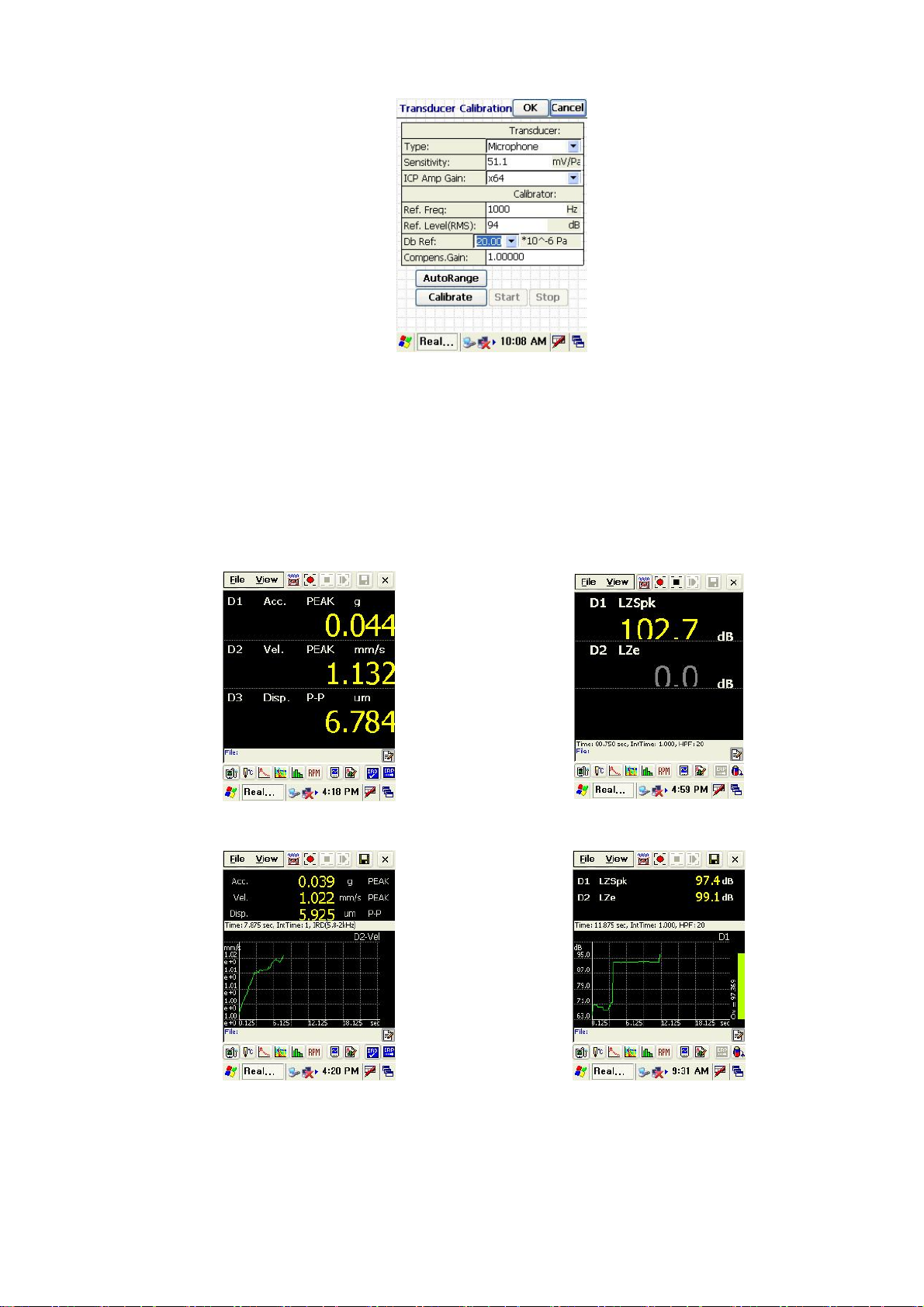
[Fig. IV-2-16] Setting the reference of decibel in SLM

2. 4 Display

You can choose one detector among 3 detectors in Vibration Level Meter mode and among 2
detectors in Sound Level Meter mode in the [Detector] of [Display] Option. You can see 4 types­[None], [Trace], [Octave], [FFT]-graph as display option from [Fig. IV-2-17] to [Fig. IV-2-21]

[Fig. IV-2-17] Display-None in VLM

[Fig. IV-2-18] Display-None in SLM

[Fig. IV-2-19] Display-Trace in VLM

[Fig. IV-2-20] Display-Trace in SLM

31

[Fig. IV-2-21] Display-FFT in VLM

But octave and FFT graph is shown only in the WBCombined Filter. The 1/1, 1/3 and 1/6 Octave
analysis which is selected in FFT option window is supported. So after you changed to FFT mode,
you have to press the FFT option button
the chapter V-5.

The FFT and Octave Graph of the Vibration Level Meter are supported in the
Human Vibration Filter, BW 1.6kHz, BW 200Hz and BW 100Hz. They are not
supported in another Filter. Also, the option of octave is set in the FFT option
window.

to set octave. If you want to see the detailed contents, see

[Fig. IV-2-22] Display-Octave in VLM

3. Display Option

3. 1 Trace Graph

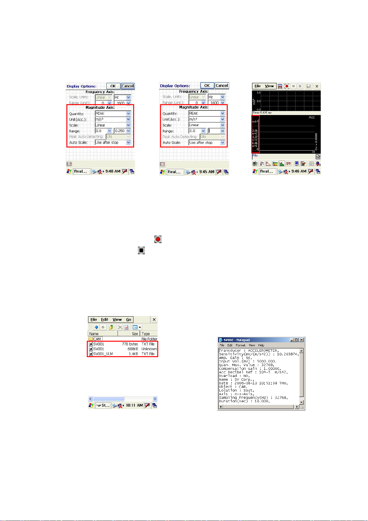
If you press the
red square is only for vibration level meter. The range of y-axis in the trace graph is defined at
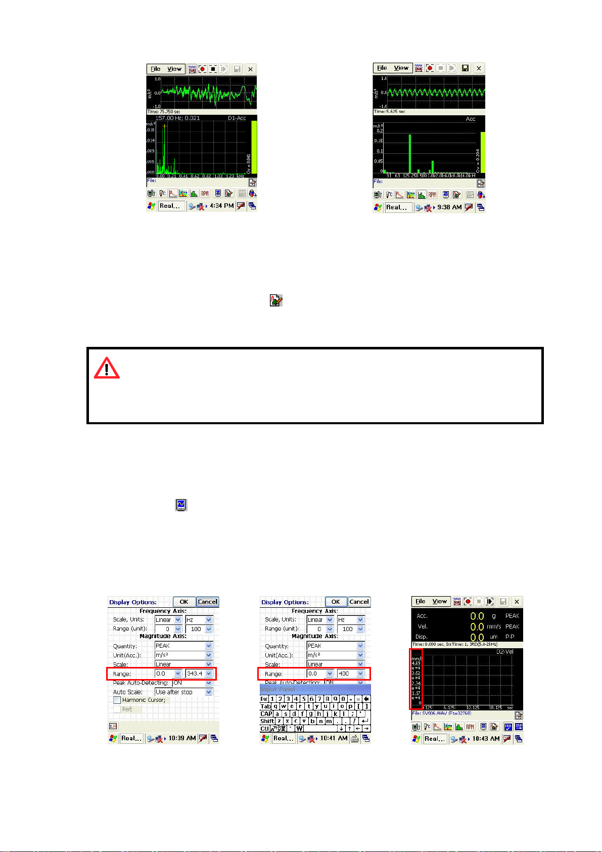
[Range] as [Fig. IV-3-1] or you can input this range with keyboard. If user clicks the Y-Axis by
stylus pen, the range of Y-Axis is automatically adjusted.

[Fig. IV-3-1]Adjustment of

the range of trace

button, the display option window appears as [Fig. IV-3-1]. The option in the

[Fig. IV-3-2] Entering the

range of trace with keyboard

[Fig. IV-3-3] Auto-scaling for

y-axis

32

3. 2 Octave graph

Control of octave graph is similar to controlling trace graph. For more detailed information about

the control, see the pictures from [Fig. IV-3-4] to [Fig. IV-3-6].

[Fig. IV-3-4] Adjustment of the

scale of octave

[Fig. IV-3-5] Entering the range

[Fig. IV-3-6] Auto-scaling for

y-axis

4. Measurement and Storage

Measurement starts with pressing button. If you don’t use [Timer] or [Integration Time] option,
you have to press stop button
with measurement option and text file with vibration level. Saving the wave file depends on [Save
Wave File In VLM / SLM] option in [File>>Recording Options…] tap. If you check the saving option,
a wave file will be saved. Otherwise, a wave file exists without data.

If you want to get more information, see the chapter III-6.

for stopping. Stored files are three which are a wave file, text file

[Fig. IV-4-1] The Three Saved Files

[Fig. IV-4-2] File with Measurement

Information

33

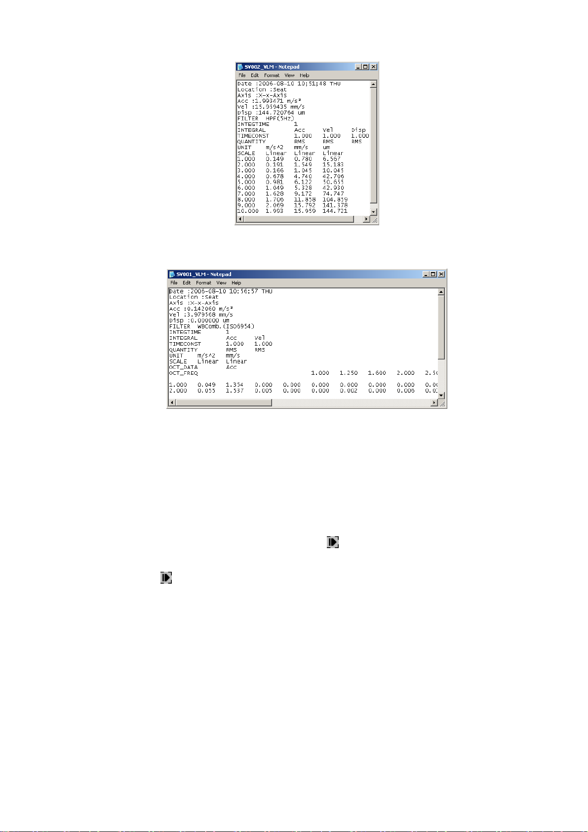
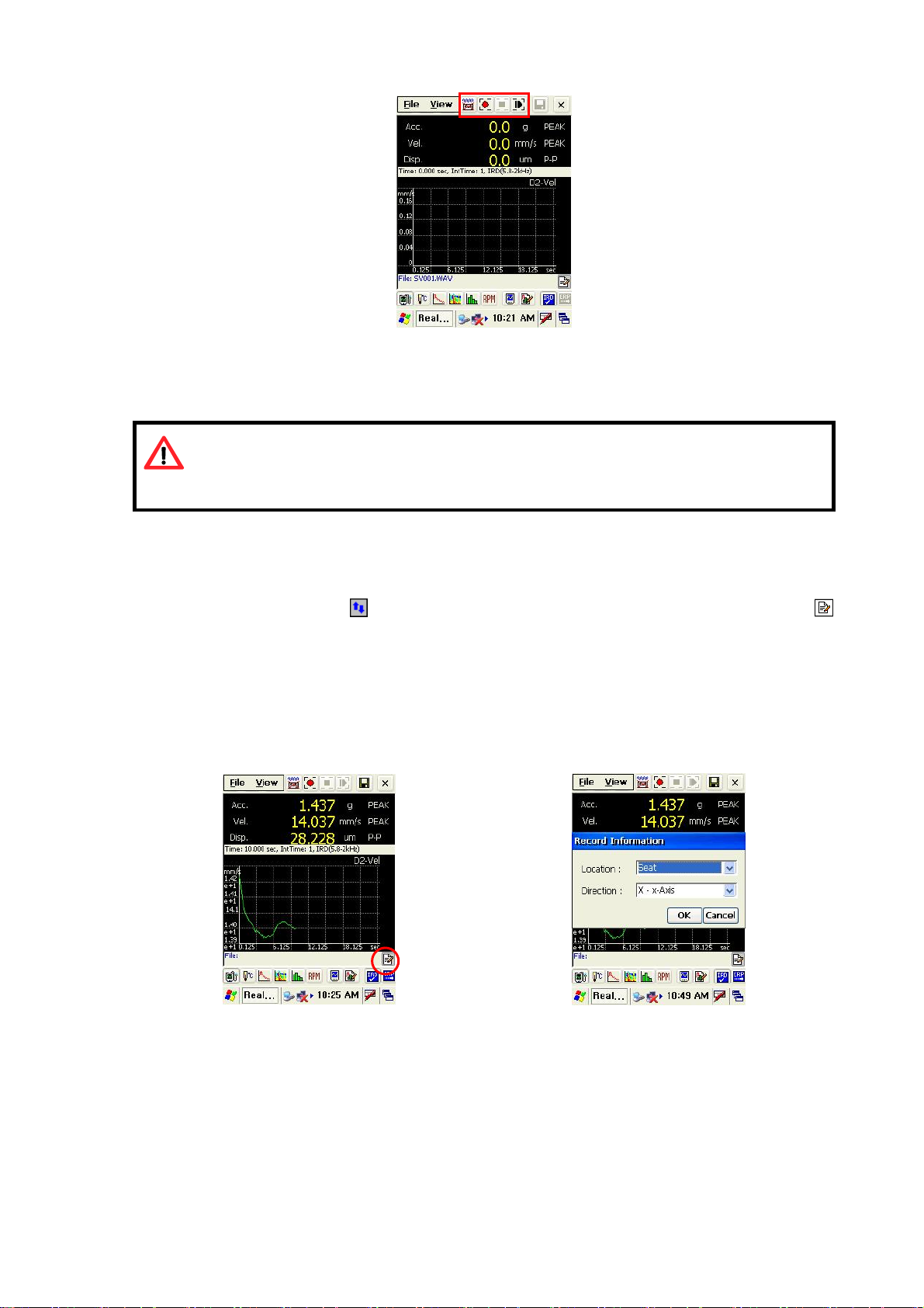
[Fig. IV-4-3] File with Vibration Level

[Fig. IV-4-4] File with Vibration Level and Octave Results

If you want to get results with vibration level and octave data together as [Fig. IV-4-4], you should
set the octave graph at [Display] in vibration level meter.

5. Playback and Analysis

You can play the wave file using playback button after opening (or loading) wave file. The
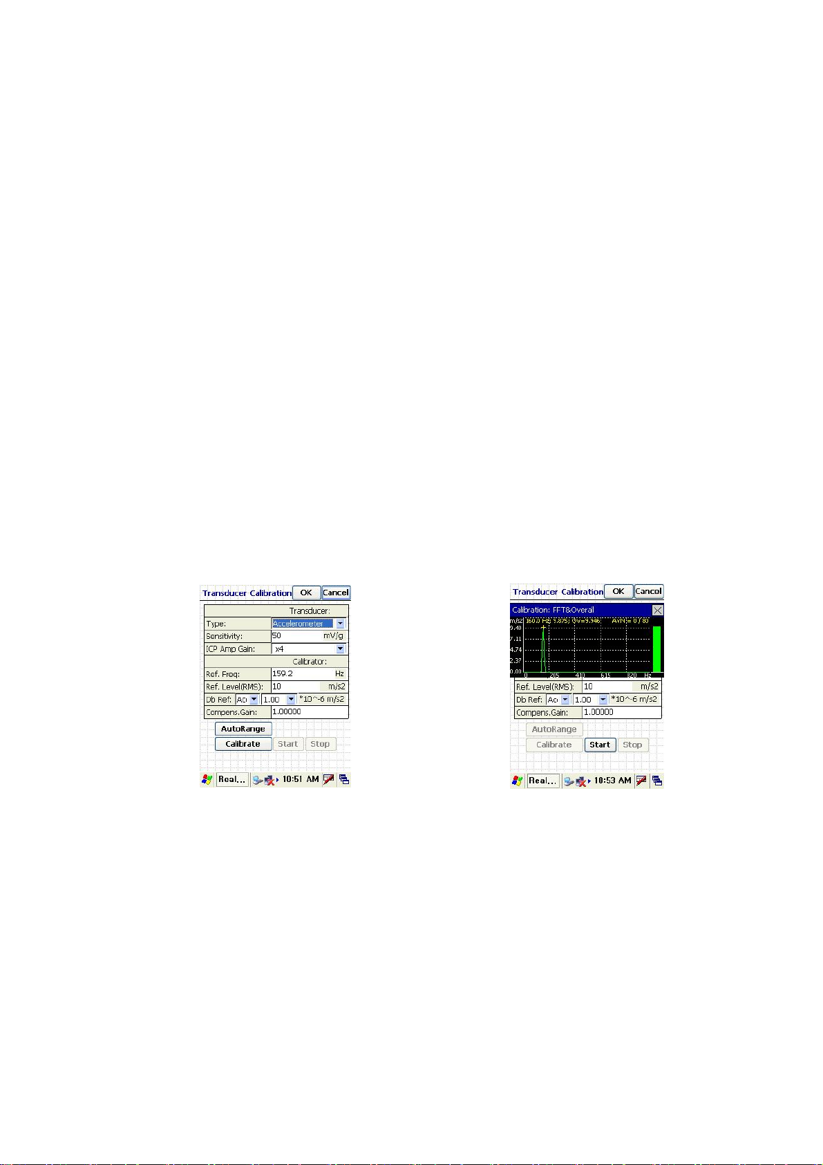
measured wave file is so loading basically that you can play that without loading (see [Fig. IV-5-1]).
Playback button
wave file as the measured options. If you play wave file again, the results of analysis are overwritten
at every playing.

is activated always when wave file is loading. The analysis is carried out playing

34

[Fig. IV-5-1] Playback Button is Activated after Loading Wave File

Measured and Analyzed Data File is overwritten at every playback. If you want
to analyze with another option and playback, you have to change the results file
name absolutely.

6. Input of Measurement Information

Press toolbar switch button in red circle of [Fig. IV-6-1] after measurement. You can see
button which is measurement information input button. If you click it, dialog box appears for
selecting the information of measurement as [Fig. IV-6-2]. Texts (or Information) of dialog box are
inputted previously in [File>>Recording Informations…] option. Also the information is written in
the result file of vibration level.

[Fig. IV-6-1] Measurement Information Button

[Fig. IV-6-2] Selection of Measurement

Information

7. Octave Analysis in Vibration Level Meter

The option of octave analysis in the human vibration filer of vibration level meter is listed below :

- Sampling Frequency : 512Hz
35

- Buffer Size : 2048

- Hanning Window

- Exponential Averaging : Time constant is same to that of detector.

- Frequency Range : 1~100Hz

- Nth Octave : 1/1, 1/3, 1/6 Octave is useful. This parameter is changeable in [Nth Octave] of FFT
Analysis(or Spectrogram, Octave Analysis) Option.

If you want to get the more information of octave analysis, refer to the chapter V-3.

8. Setting options for Human Vibration Measurement

8.1. Selecting type of sensor, Entering sensitivity and Calibration

1 Select [Accelerometer] in [File>>Transducer Calibration…] tap.
2 Entering Sensitivity at the option [Sensitivity].
3 With connecting sensor to calibrator, click [Calibrate] and [Start] button to accomplish calibration.

> [Compens. Gain] value is changed from 1 to another value.
4 Adjustment of [ICP Amp Gain] just before measuring : With connecting sensor and adhering the
sensor at measurement position, select [ICP Amp Gain] or [AutoRange] button to set the gain
automatically.

[Fig. IV-8-1] Selecting Sensor and Entering

Sensitivity

8.2. Setting the measurement time and file name

[Fig. IV-8-2] Calibration

When selecting [File>>Recording Option…] tap, a window appears like [Fig. IV-8-3].

1 [Save Wave File in VLM / SLM] option should be checked to store wave files.
2 [Use Timer] option should be checked to use timer. Measurement for 1 minute is recommended at

ISO6954:2000(E). If main component is smaller than 2Hz, it is recommended to set the measurement
for 2 minutes.

3 Enter the file name as you wish at [File Name].
4 Select the folder at [Select Folder:]

36

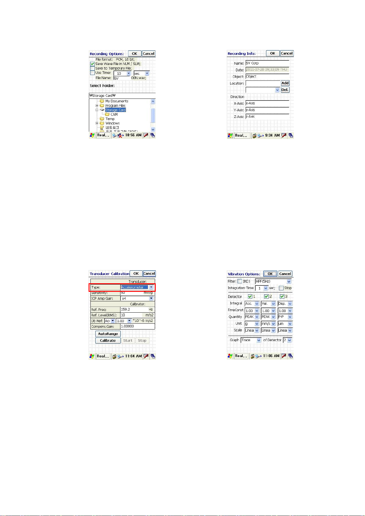
[Fig. IV-8-3] Recording Option

8.3. Entering Recording information

1 Select [File>>Recording Information…]
2 Enter name, object, location and direction of measurement in advance.

8.4. Selecting Vibration Level Meter and Setting the measurement options

1 Change the analysis mode to vibration level meter.
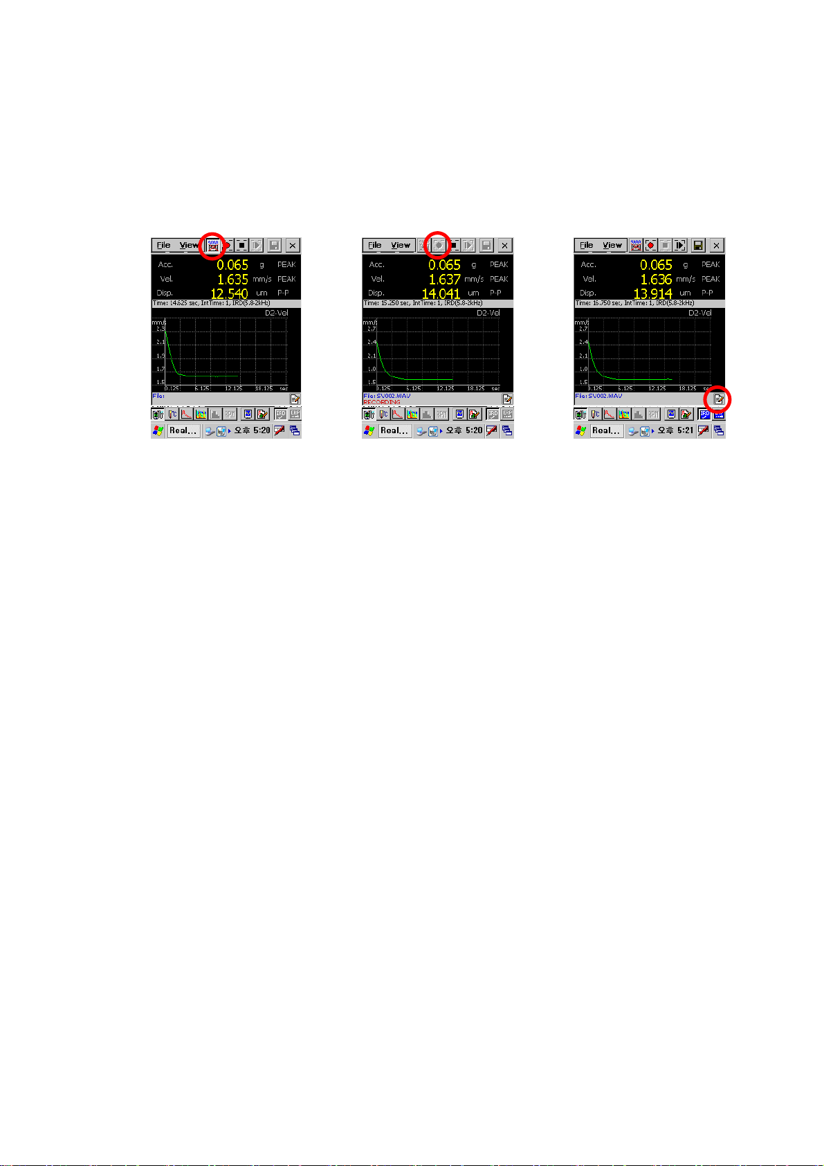
2 Select the vibration options as [Fig. IV-8-5]. Set [Integration Time] for 1 second and [Time

Constant] for 1 second. Therefore, the data is stored per 1 second for 1 minute.

[Fig. IV-8-4] Entering Recording information

[Fig. IV-8-5] Conversion of Vibration Level

Meter Mode

[Fig. IV-8-6] Window for Vibration Options

37

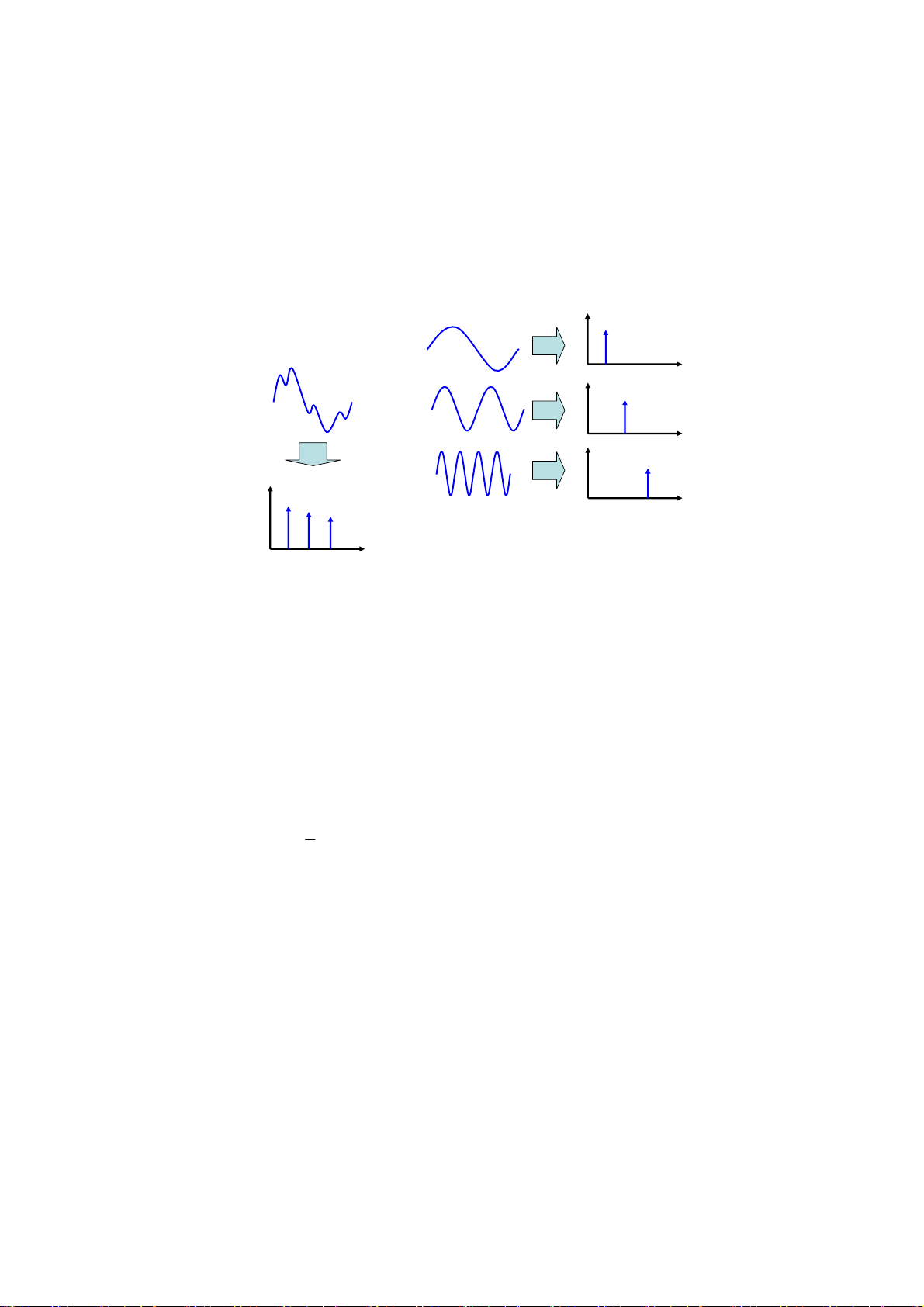
8.5. Measurement

1 Confirm the status of measurement to press [ARM] button.
2 Start measurement to press [Record] button.
3 Enter recording information to press [Entering recording information] button.

[Fig. IV-8-7] ARM Button

[Fig. IV-8-8] Recording Button [Fig. IV-8-9] Entering recording

information Button

38

x

X

V. Real Time FFT SpectrumxSpectrogram and Octave Analysis

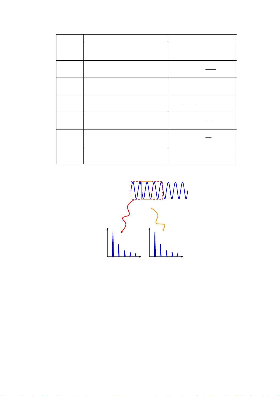
1. Understanding of Frequency Analysis

The shape of the time signal is so complex that we can’t see the information of frequency in the
measured time signal. Therefore, we have to calculate FFT (Fast Fourier Transform) analysis to get
the information of frequency-the periodicity of time signal. Frequency analysis is classifying the
magnitude of time signal as frequency like [Fig. V-1-1]

Spectrum

FFT

+

Frequency

FFT

Spectrum

Frequency

=

+

+

…

FFT

Frequency

FFT

Frequency

[Fig. V-1-1] Concept of Frequency Analysis

2. Fast Fourier Transform

Frequency analysis usually uses Fast Fourier Transform which is abbreviated to FFT. The basic
assumption to calculate FFT is that time signal has infinite periodicity. Here is the calculating
equation below :

k

N

1

−

⎡⎤

=≤≤−

[] () , 0 1

Xk xne k N

⎢⎥

∑

n

0

=

⎢⎥

⎣⎦

⎛⎞

jn

2

π

−

⎜⎟

N

⎝⎠

<Eq. V-2-1>

()

where

n

is discrete time signal, N is the buffer size of FFT. And

result of FFT. In general,

N has the number of 2

n

-512, 1024, 2048, 4096. The parameters of FFT

[]

k

is the calculated

are listed in <Table V-2-1>.

The calculation of FFT accomplishes after an allocated buffer is filled with data. This procedure is
shown in [Fig. V-2-1].

FFT is calculated after the first buffer is filled with data, and then 2FFT is

1

calculated after the second buffer is filled with data. This procedure is continuous, so we can see the
FFT results as real-time data.

39

s

s

s

F

f

s

F

s

=

<Table V-2-1> Defined Parameters for FFT

Parameters Definition Equation

F

F

pan

N

L

Δ

tΔ

T

Sampling Frequency User Definition

Useful Frequency Range

Buffer Size User Definition

Display Line

NN

LL=+ =

F =

span

1 or

2.56

2.56 2.56

Frequency Resolution

Sampling Interval(sec)

fNΔ=

t

Δ=

1

F

Recording Time

or Total Time of Saved Data in Buffer

Buffer 1

Buffer 3

TNt

⋅Δ

Buffer 2

Freq Freq

FFT of Buffer 1 FFT of Buffer 2

[Fig. V-2-1] Instantaneous FFT results from each FFT calculation

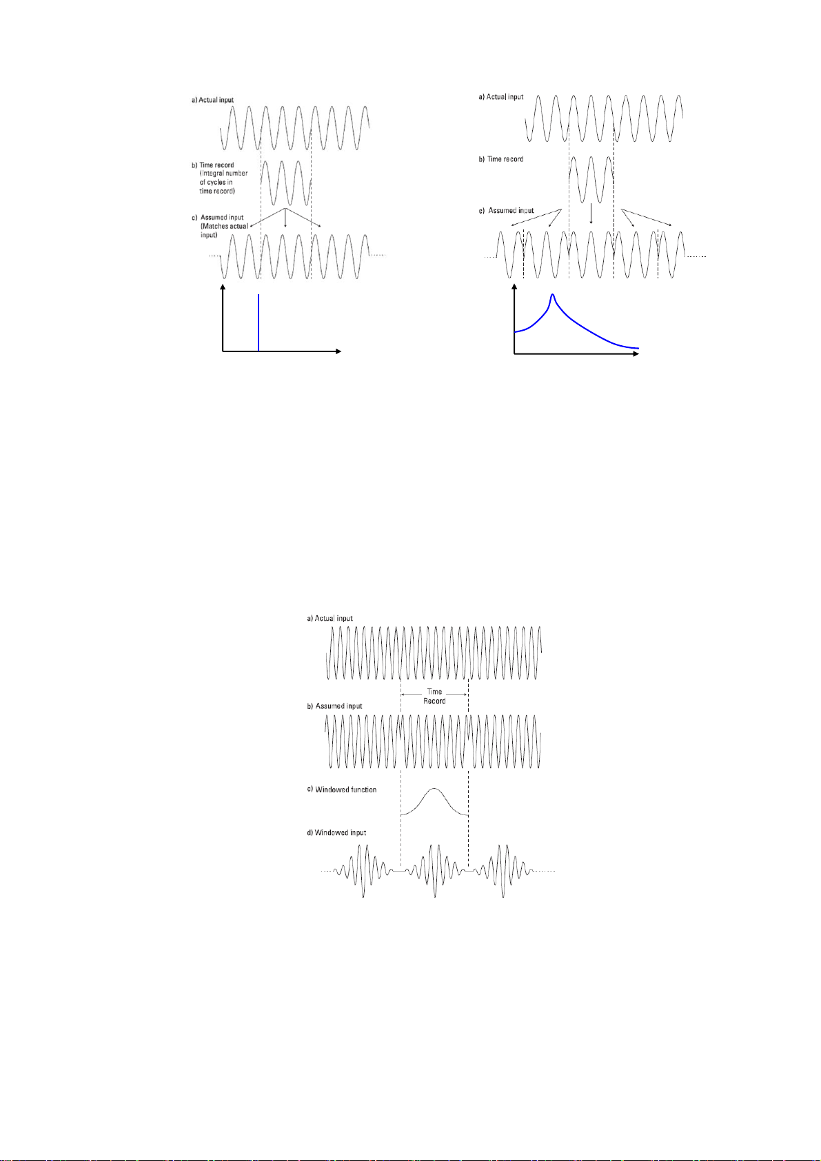
As previously mentioned, the basic assumption of FFT analysis is that time signal has infinite

periodicity. But buffer size is so finite that energy leakage causes. So we call it “leakage error”. As
shown in [Fig. V-2-2], time signal with infinite periodicity generates just one peak in FFT results.
However, as shown in [Fig. V-2-3], time signal with finite buffer causes finite periodicity. If we
calculated FFT using this buffer, we got the broaden peak of FFT.

40

x

[Fig. V-2-2] Ideal FFT

Freq

[Fig. V-2-3] Actual FFT

Freq

2. 1 Windowing

We must use windowing function to solve leakage error. The procedure shown in [Fig. V-2-4] is the
windowed time signal which is original time multiplied by windowing function. The figure (b) is
shown the finite periodicity of time signal that is recognized in FFT algorithms, but figure (d)
represents the infinite periodicity of time signal by multiplying original time signal and windowing
function. Therefore, a windowed time signal has not leakage error.

[Fig. V-2-4] Windowing Procedure

Windowing is multiplied time signal and the coefficients of window which has number

N

. Here is

the equation below :

() () ()

iwixi=×, 01iN≤≤ − <Eq. V-2-2>

w

41

x

x

x

x

x

x

F

F

F

F

where

N

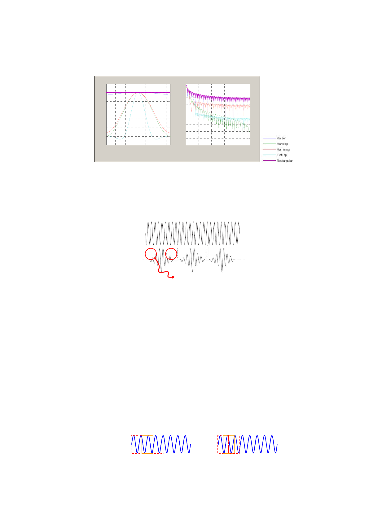
is buffer size. There are all kinds of window function, but generally hanning, flat-top and

rectangular(no window) window is used.

1.2

1

0.8

0.6

0.4

Amplitude

0.2

0

-0.2

Time domain

10 20 30 40 50 60

Samples

40
20

0

-20

-40

-60

Magnitude (dB)

-80

-100

-120

-140
0 0.2 0.4 0.6 0.8

Frequency domain

Normalized Frequency (×π rad/sample)

[Fig. V-2-5] V arious Windowing Functions

However windowing causes the leakage of time signal’s energy as [Fig. V-2-6].

Energy Leakages

[Fig. V-2-6] Windowing causes the leakage of energy of time signal

2. 2 Overlap

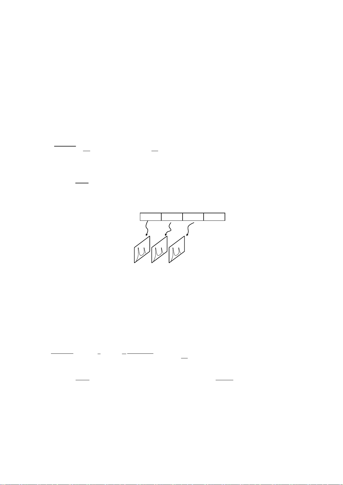
Overlapping is done to protect energy leakage. If you hope to understand the overlapping, you have
to know no overlapped time signal. For example, let’s suppose that the first time data
the second time data
the FFT spectrum of

has N ~ 2N-1 and so on.

2

. See [Fig. V-2-7]. The left figure is no overlap that means the time signal

2

FFT is the FFT spectrum of

1

buffer for FFT is not repeated. 50% Overlapping uses the second half data of
data of

together.

2

has 0 ~ N-1,

1

and

1

and the first half

1

FFT is

Over 66% overlapping doesn’t usually have the loss of energy in the time signal.

FFT

1

No Overlap

FT

2

FT

FFT

3

1

50% Overlap

FT

2

FT

3

2

[Fig. V-2-7] Overlapping

42

F

F

F

−

τ

2. 3 Averaging of FFT Spectrum

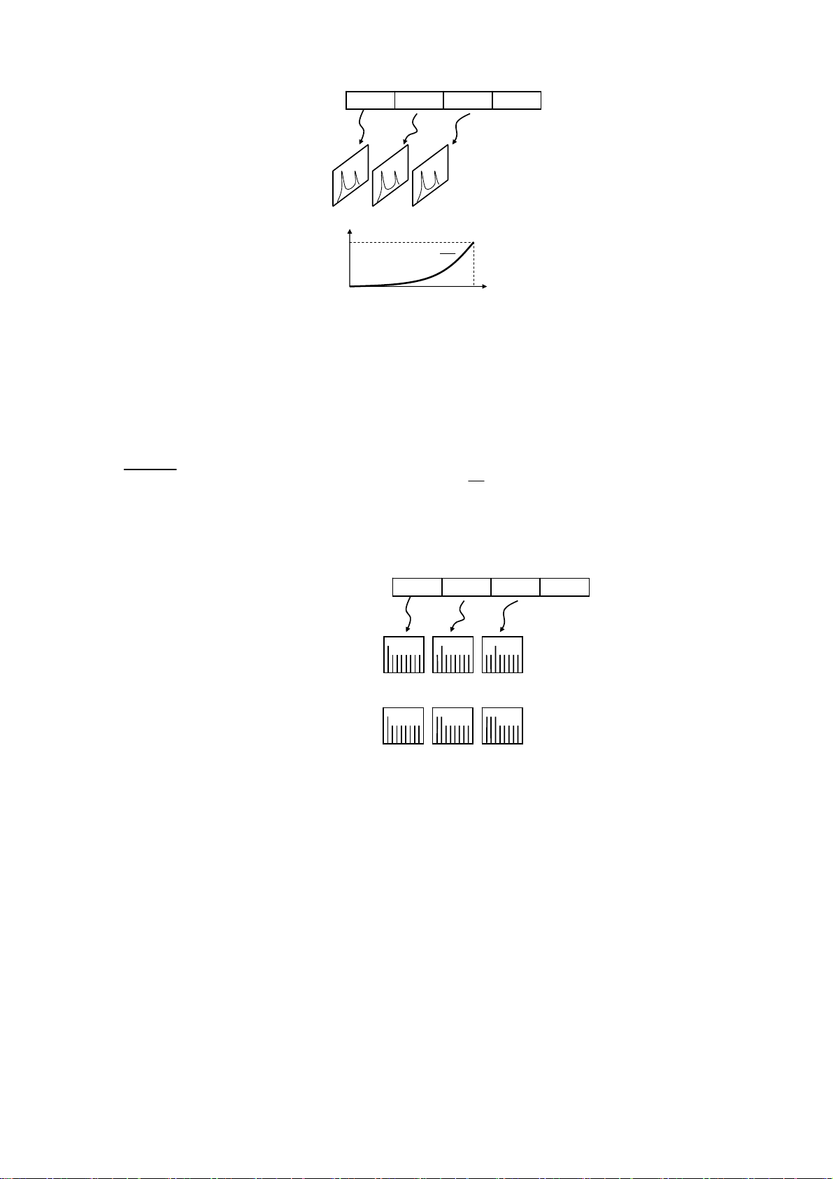
The reason of averaging spectrum is to remove noises in the spectrum. There are linear averaging,
exponential averaging and peak hold averaging.

2. 3. 1 Linear Av eraging

Let’s suppose that

FFT is FFT spectrum of the first time signal buffer, 2FFT is FFT spectrum

1

of the second time signal buffer and so on as [Fig. V-2-8]. Linear averaging is the arithmetic average
of spectrums at each frequency. On other words, you have to sum all of spectrums at special
frequency, and then divide summed values with averaging number like the equation below.

n

a

() ()

FFT k FFT k

1

=

∑

n

i

1

=

a

, 0

i

N

k≤≤ <Eq. V-2-3>

2

where

FFT is the averaged spectrum of FFT. an is averaged number.

N

is buffer size.

Time1

Time2 Time3

…

FFT1FFT2FFT

3

[Fig. V-2-8] Instantaneous FFT Spectrum

2. 3. 2 Exponential Averaging

Exponential averaging is calculated from the exponential averaged spectrum at each frequency
using <Eq. V-2-4>. Exponential averaging emphasizes recent spectrum in all of spectrums.

⎛⎞

FT k e e FFT k

⎜⎟

ii

=− ⋅

() 1 ()

⎝⎠

where

spectrum.

FT

T is the total time of one buffer per second. And

ττ

∑

=

0

i

is the averaged spectrum of FFT at present.

i

, 0

−

1

N

k≤≤ <Eq. V-2-4>

2

FT

is the proceeding averaged

1i

is time constant per second.

TiT

∞

−−

43

]

≤

time

…

Time1

FFT1FFT2FFT

Time2 Time3

3

−t

τ

τ

e

[Fig. V-2-10] Exponential A veraging

2. 3. 3 Peak Hold Averaging

This averaging keeps the biggest peak value of spectrum at the same frequency to repeat with
averaging number. This theory is shown in [Fig. V-2-10] and <Eq. V-2-5>.

N

() ()

FFT k MAX FFT k= , 01

[

i

in≤≤ −, 0

a

k

≤ <Eq. V-2-5>

2

where

n is averaging number(or iteration number for averaging).

a

Time1

Instant FFT

FFT1FFT2FFT

Averaged FFT

FFT

Time2 Time3

FFT2FFT

1

3

3

…

[Fig. V-2-10] Peak Hold Averaging

2. 4 Picket Fence Error

The resolution of frequency is defined as dividing the sampling frequency by buffer size. Therefore,
if the peak of spectrum exists in the smaller region than resolution, the peak was not shown with real
value. The energy of peak divides into both side spectrums. In this situation, we can’t get a real
frequency and magnitude of peak. This is called ‘Picket Fence Error’. This error is shown in [Fig. V­2-11]. If you want to get the exact frequency and magnitude of spectrum, you have to compensate
both parameters with some theory.

44

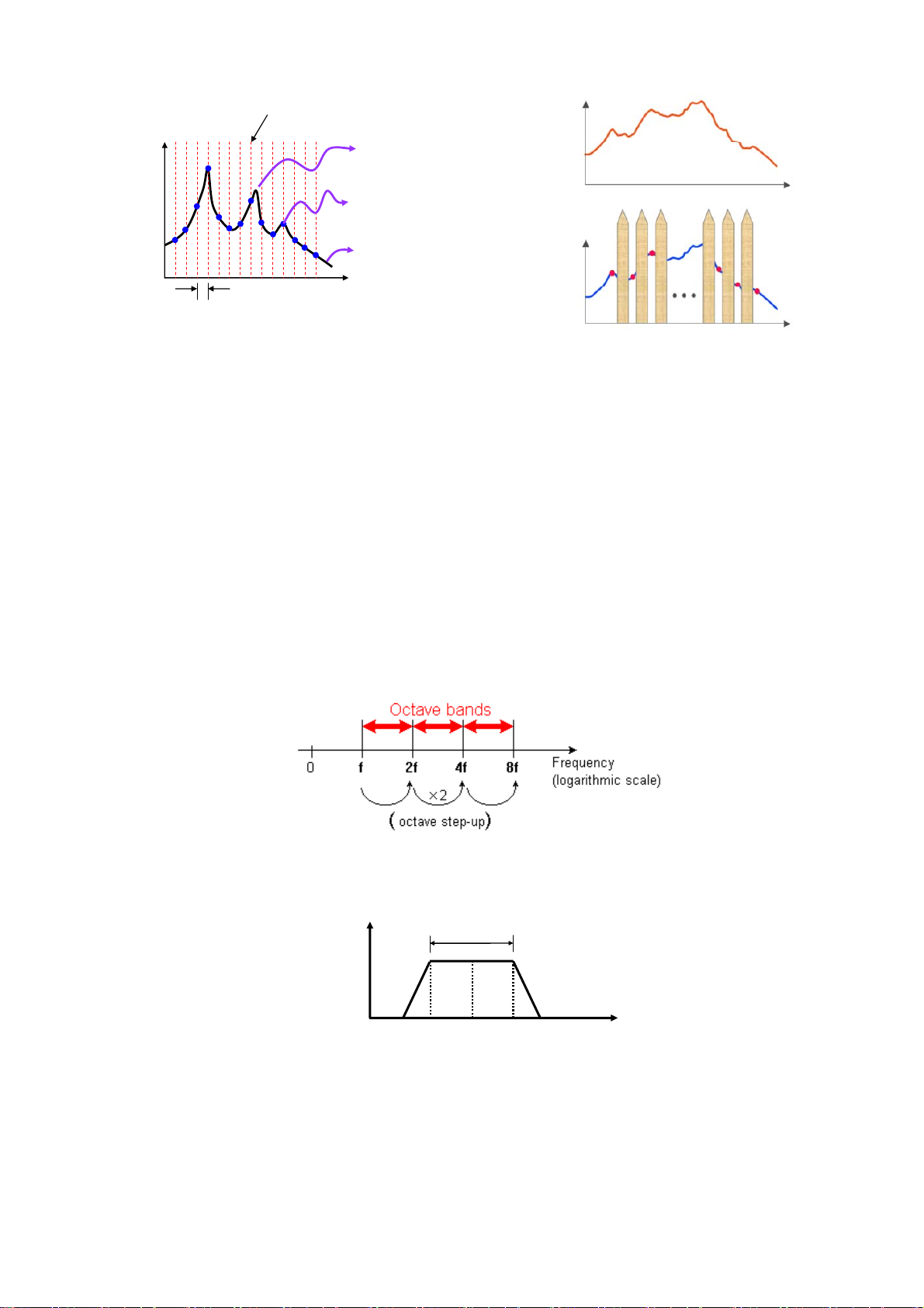
Display Line

This real peak is not shown in
graph

This points are disp l ayed in
the graph

Real Spectrum

Freq

fΔ

[Fig. V-2-11] Picket Fence Error

3. FFT Based Octave Analysis

FFT analysis is named narrow band frequency analysis, but octave analysis which is describing in
this paragraph is called broad band analysis. Octave means the twice frequency of reference’s
frequency. Reference frequency is defined as 1kHz in the International Standards-ANSI S1.11.
Therefore, we can make bandpass filters with center frequency which is based on octave of 1kHz.

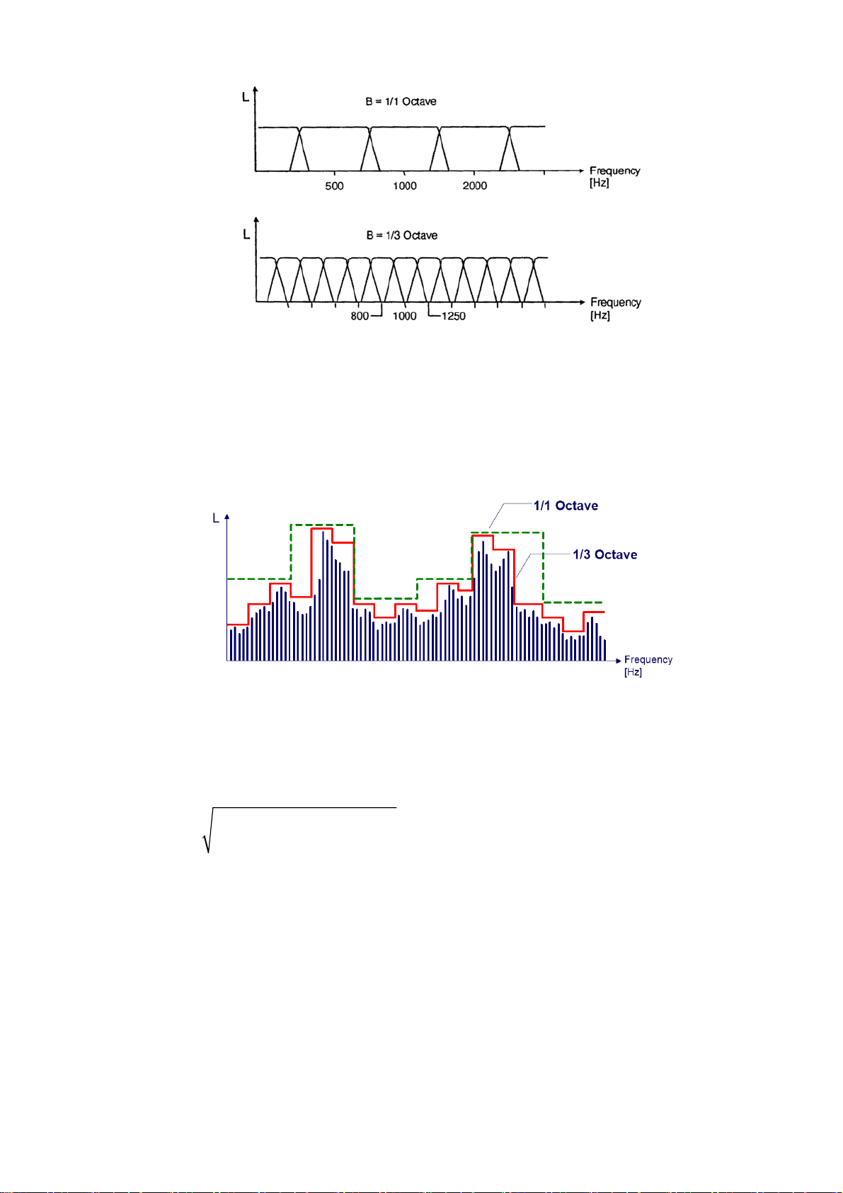
Octave analysis uses a lot of defined bandpass filter. The 1/1 octave bandpass filter with 1kHz
center frequency is shown in [Fig. V-3-2]. This 1/1 octave filter means bandpass filter with a full
octave band. 1/3 octave filters are realized by bandpass filter with bandwidth that is divided an octave
by 3. Therefore, you can get 1/1 octave data from 1/3 octave data.

[Fig. V-3-1] Concept of Octave

=708

f

l

Bandwidth

fc=1000

=1410

f

u

Frequency

L

[Fig. V-3-2] 1/1 Octave Based Bandpass Filter with 1kHz Center Frequency and an octave bandwidth

45

y

[Fig. V-3-3] 1/1 and 1/3 Octave Bandpass Filters

1/1 and 1/3 octave bandpass filters are shown in [Fig. V-3-3]. As previously mentioned, we can
calculate the octave data from FFT spectrum. The relationship is shown in [Fig. V-3-4].

[Fig. V-3-4] Relationship between FFT Spectrum and Octave Analysis

Equation for calculating is <Eq. V-3-1>.

/2

N

yy

1/3

where

=⋅

Octave i

is the spectrum of FFT.

i

∑

i

=

2

Window Correction

0

<Eq. V-3-1>

y is the octave value of each band. i is frequency index

1/3Octave

in the spectrum.

4. Weighting

Microphone is reacted uniformly as the frequency of sound. So when you measure the sound using
a microphone, you can’t get the sound level as you hear the sound because the ear of hu man being
hears sound differently according to the frequency.

Equal Loudness Contour represents the curve that the human being feels equal loudness of sound

46

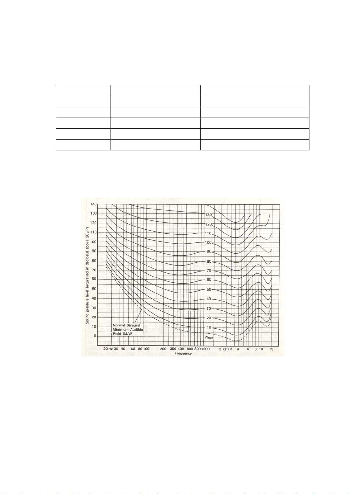
as frequency at specific sound pressure level(SPL). Sometimes, Phon unit is used instead of SPL.
Phon is same to the SPL at 1kHz. For example, the curve passing on 80dB at 1kHz is called ‘80phon
curve’. The definition of weighting functions is listed in <Table V-4-1>.

<T able V-4-1> Various Weightin g Filer

Weighting Term Curve Definition Remarks

A-weight Reciprocal of 40phon Curve Useful in Noise Analysis
B-weight Reciprocal of 70phon Curve ­C-weight Reciprocal of 100phon Curve ­D-weight - Useful in Airplane Noise Analysis
E-weight - -

Normal Equal Loudness Contour is shown in [Fig. V-4-1], the frequency responses of each

weighting function are shown in [Fig. V-4-3].

[Fig. V-4-1] Normal Equal Loudness Contours

47

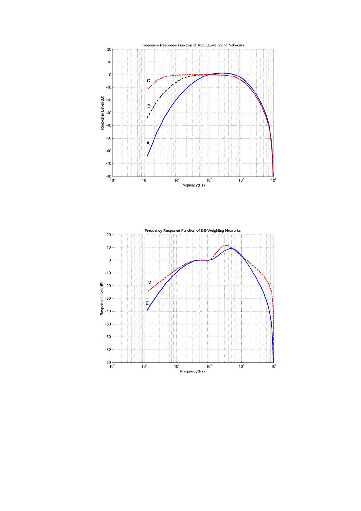
[Fig. V-4-2] A, B, C-Weighting Frequency Response

[Fig. V-4-3] D, E-Weighting Frequency Response

5. Integration in Frequency Domain

Velocity and displacement spectrum can be analyzed in FFT and Octave, Spectrogram analysis
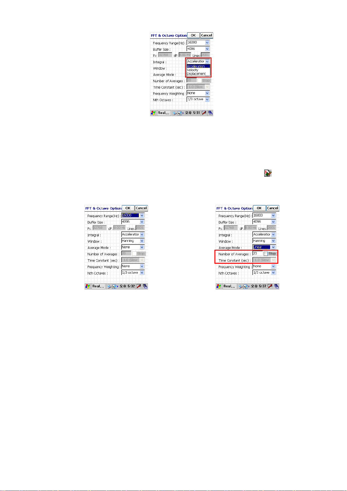
when accelerator is used. For this, you select [Integral] option in [Fig. V-5-1]. The detailed theory of
integral in frequency domain sees [VI. 3. 2] verse.

48

s

[Fig. V-5-1] Integration in Frequency Domain

6. Setting the Options of Measurement

Setting the options of measurement of frequency analysis, spectrogram and octave analysis is
defined in the same option’s window. If you press ‘FFT & Octave option’ button

, the window of

[Fig. V-6-1] appears.

[Fig. V-6-1] Setting the Option for FFT Analysis

[Fig. V-6-2] Inputting Averaging Number or

Time Constant

Frequency range means the useful frequency and is same to frequency span as mentioned. The
maximum of frequency range is 16 kHz. Sampling frequency

F is dependent on the frequency span

and maximum value is 32768Hz. You have to also choose the buffer size which has the max 4096. A

dF

frequency resolution(

) is dependent on the relationship between sampling frequency and buffer

size. The number of lines is dependent on the buffer size.

The relationships of parameters are listed in <Table V-2-1>.

Window function is supported with rectangular, hanning and flat-top window. Average mode is
offered with NONE, linear and exponential averaging, peak hold averaging. If you select the linear or
peak hold averaging, the box for number of average is activated. The system with [ Stop] will stop
measuring automatically when the numbers of average reaches the input number. If you set [Use
Timer] in [File>>Recording Options…] and [ Stop] simultaneously, the system will stop at short
time.

49

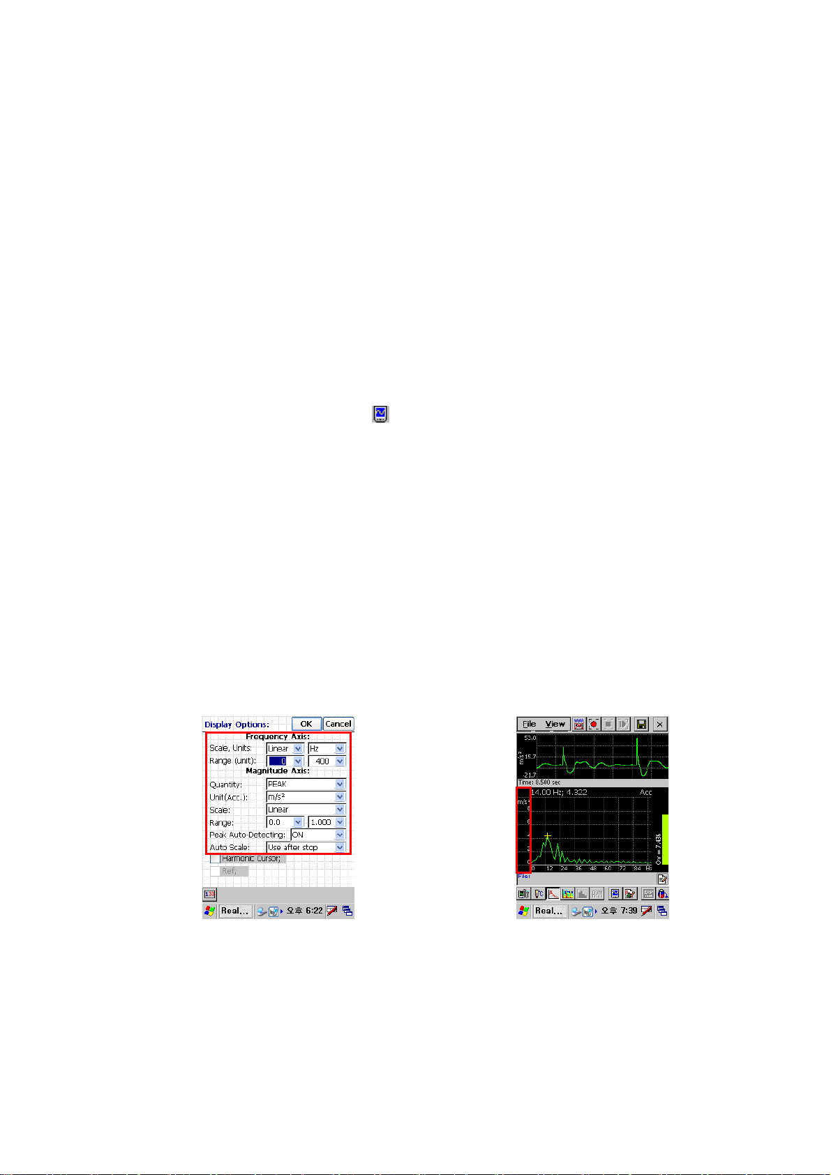
Selecting the exponential averaging have been activated the combo box of time constant. You can
choose the proper time constant and this function doesn’t offer the automatic stopping with [ Stop].

Frequency weighting is used to analyze the noise with A, B, C, D, W weighting filter. A-weighting
is an ordinary weighting in noise analysis. The combo box of [Nth Octaves] has 1/1 octave, 1/3
octave and 1/6 octave.

FFT based octave analysis is dependent on the options of FFT analysis. So you have to set the
option of FFT properly. For example, if the linear averaging with 20 iterations is set, octave analysis
is calculated from linear averaged spectrum with 20.

7. Setting the option of display

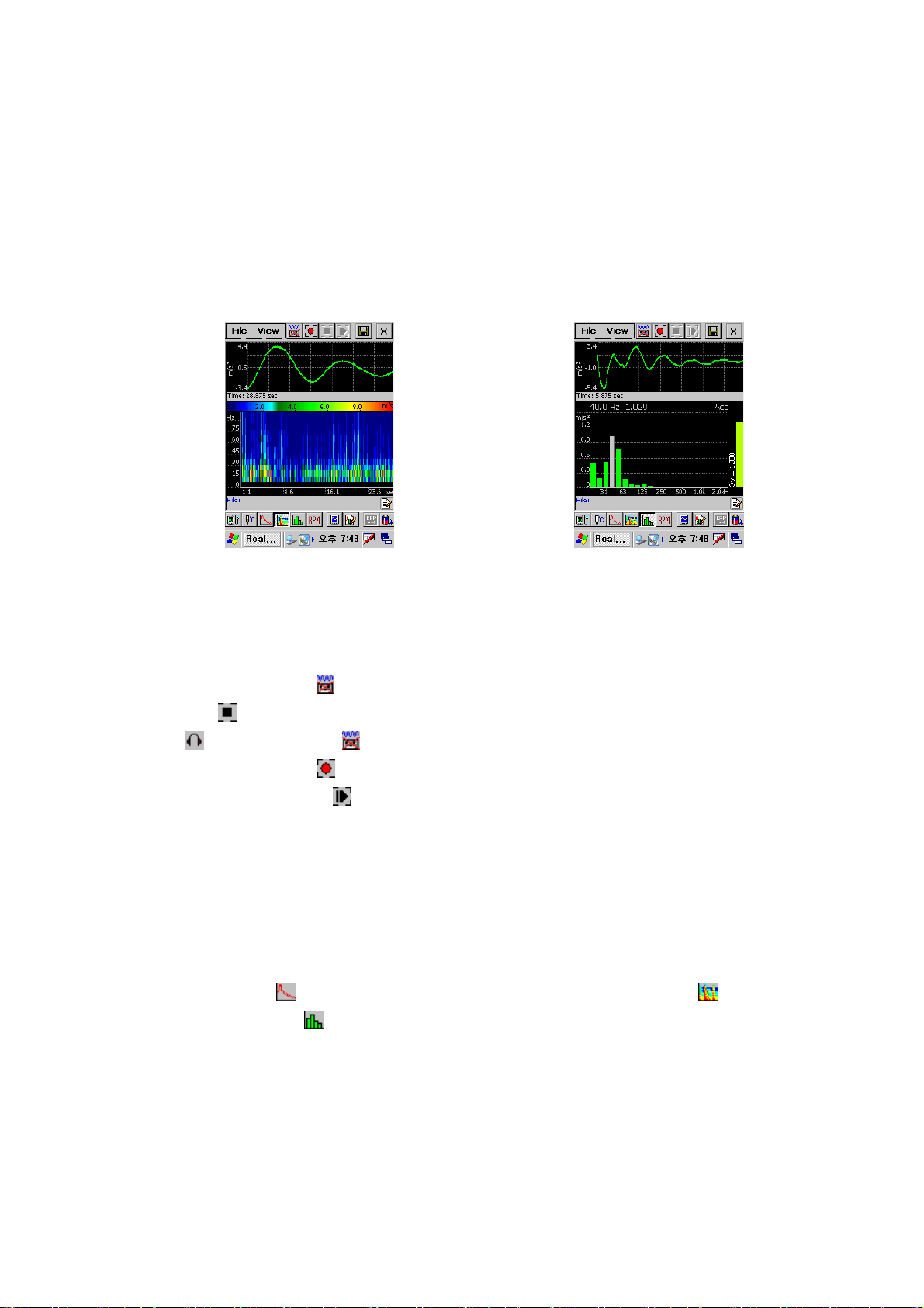
Pressing the display option button generates the window of [Fig. V-7-1]. The adjusting
frequency and magnitude axis is used in frequency analysis, spectrogram and octave analysis. The
range of frequency axis defines the start frequency and end frequency in the FFT graph. And the scale
of frequency axis is defined linear axis or logarithms axis. Frequency range is editable in linear scale,

but it is impossible in logarithms scale. The units in magnitude axis is displayed with RMS(

Pa ) , Peak(

2

/ms or Pa ), Power(

24

/ms or 2Pa ) and scale is displayed with linear / logarithms /

2

/ms or

decibel scale.

For example, if you want to see the decibel of RMS value, you have to set that the unit is RMS and
the scale is dB.

There is another way for adjusting magnitude axis. If user clicks the Y-Axis by stylus pen, the
range of Y-Axis is automatically adjusted.

[Fig. V-7-1] Option Window Display

[Fig. V-7-2] Auto-scaling of Magnitude Axis

Cross marker represents the maximum peak of spectrum with frequency and magnitude after [Peak
Auto-Detecting] is turned on. And if you press any peak of FFT graph for 1second, big cross marker
appears with current frequency and magnitude instead of the value of peak auto-detecting. Pressing
the screen for a short time turned off that function. The rightmost bar graph is overall level.

50

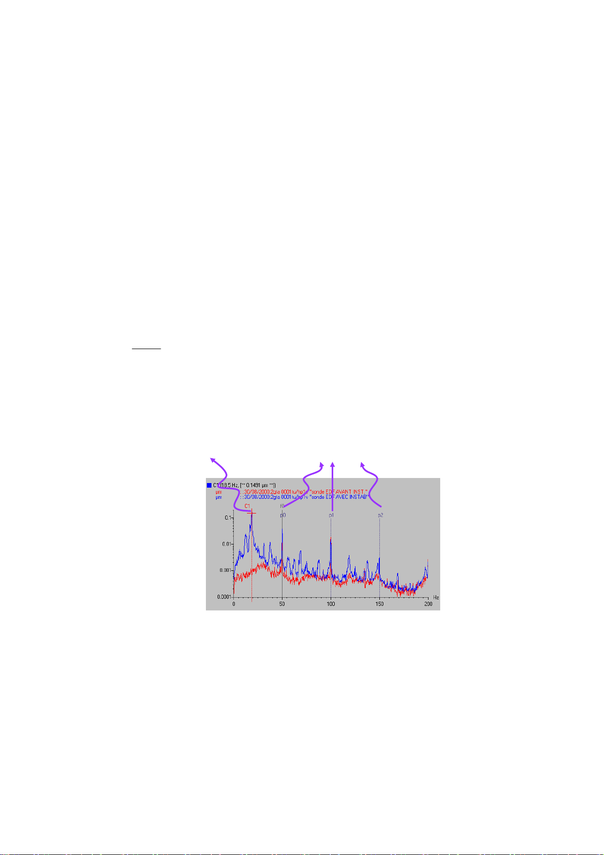
[Auto Scale] and [Peak Auto-Detecting] function is not offered and only the adjustment of
frequency is available in the spectrogram graph.

In octave analysis, [Auto Scale] function is offered but [Peak Auto-Detecting] function is not
offered. However, the bandwidth being pressed for 1 second is changed from green to white bar, and
then you can read frequency and magnitude in the leftmost top of octave graph. Refer to [Fig. V-7-4].

[Fig. V-7-3] Spectrogram Graph

[Fig. V-7-4] Octave Graph

8. Record and Playback

Press the ARM button to see an analyzed data in real-time without recording. And press the
stop button
button

Press the record button
loaded and playback button
analyzing the data executes at the same time.

To export a measured data, [Export] menu in [File>>Export…] tap should be selected. Refer to the
chapter III-4 to get the details.

to stop arming. If you want to hear the sound in real-time, you have to press hearing

and arming button simultaneously.

to record and analyze the data. After recording is finished, wave file is

is activated. If you press playback button, playing the wave file and

9. Mode Conversion of FFT Analysis, Spectrogram and Octave Analysis

Press FFT button for frequency analysis, and press th e spectrogram button for spectrogram
and press octave button
vibration level meter mode.

for octave analysis. Recording, playback and hearing function is same to

51

R

VI. FFT Based RPM Meter

1. Understanding about the RPM Measurement

The RPM is usually measured using a tachometer. Tachometer counts the revolution of a rotator
using optical sensor and reflector or using the photo coupler and the hole of rotator or magnetic
sensor and the teeth of rotator. Anyway, all of this method contacts a rotator directly. This is good way
to get an exact revolution. On the other hand, it is a defeat. To solve the defeat, we have devised the
FFT based RPM meter.

Spectrum in a rotational vibration has a peak which corresponds to RPM and a lot of peaks against
to rotor/teeth/bearing. But a first peak generates by an input rotation. Therefore, this peak is called
‘1st order’. The peaks which is an integer times of the frequency of a first peak are called harmonic
components.

The relationship of frequency and RPM represents in <Eq. VI-1-1>.

Freq =

PM

<Eq. VI-1-1>

60

where RPM is the abbreviation of a revolution per minute. Therefore, we can calculate RPM from

the first frequency of FFT spectrum.

First Frequency

[Fig. VI-1-1] Fundamental Frequency and Harmonic Frequency

Harmonics

2. Frequency Analysis

Frequency analysis is done with the listed option below and user can’t change the option.

- Hanning Window

- Linear Averaging : this parameter is defined at [Average Number] in option setting window.

- Buffer size for FFT is variable as the maximum RPM. Refer to <Table VI-2-1>
52

<Table VI-2-1> Relationship of Maximum RPM, Sampling Frequency and Buffer Size

Max. RPM Sampling Frequency(Hz) Buffer Size

12000 512 1024
24000 1024 2048
48000 2048 4096
96000 4096 4096

As mentioned in V-2-4 paragraph, a frequency analysis generates a picket fenc e error. We can’t get
an exact frequency which corresponds to rotational RPM. As this problem, the system has a
compensation algorithm.

3. Measuring with RPM Meter

Button changes another mode into RPM mode and, at the same time, RPM option setting
button is activated. This mode doesn’t offer the recording except arming.

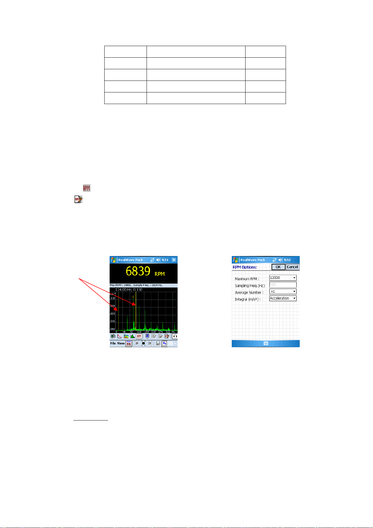
RPM Meter has the RPM window and FFT graph window as [Fig. VI-3-1]. FFT graph window has
two vertical lines for setting range of a first frequency. To calculate RPM from the maximum peak in
a defined region by two vertical lines, you have to drag lines with stylus pen.

Two vertical lines

[Fig. VI-3-1] RPM Meter

The option setting window is shown in [Fig. VI-3-2] and maximum rpm and averaging number
shall be selected. Sampling frequency is calculated from maximum RPM as <Eq. VI-3-1> equation.

[Fig. VI-3-2] Option Setting Window

.

If you set an unfit range, you would get a fault RPM from a fault frequency.

Max RPM

F

=× <Eq. VI-3-1>

s

Cross mark ‘+’ represents the maximum value in all frequency with no correlation of vertical lines.

60

2.56

53

f

f

f

3. 1 Using the Velocity Graph or Displacement Graph to get a fit RPM

It is difficult that you find the fundamental frequency in the harmonic frequency of spectrum of
acceleration. The spectrum of rotational vibration with the fluctuation from 1610PRM to 1660RPM is
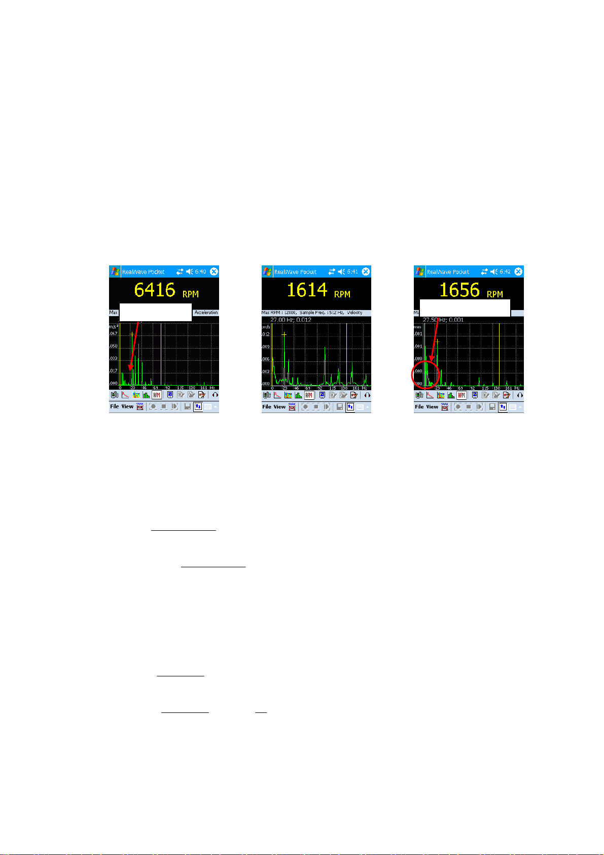
shown from [Fig. VI-3-3] to [Fig. VI-3-5]. As shown in [Fig. Vi-3-3], you can’t find the first order(or
fundamental frequency) easily and harmonic frequencies are so big that the calculated RPM is not
correct. If you find in the spectrum of a velocity or displacement, you can find it easily. But in the
integrating process, the noise of a low frequency is amplified. Consequently, though you see a first
order, you can be mixed between noise and first frequency. To solve this problem, the highpass filter
with 4Hz cutoff frequency is used. In other words, the frequency less than 4Hz has 0 magnitudes.

To get the graph of acceleration/velocity/displacement, you can set it in [Integral] of [Fig. VI-3-2].
A magnitude has RMS, units is fixed with

2

/ms, /cm s and mm.

First Order

[Fig. VI-3-3] Acceleration

[Fig. VI-3-4] Velocity

Amplified Noise

[Fig. VI-3-5] Displacement

3.2 Integral in the spectrum of FFT

The relationships of acceleration, velocity and displacement are listed below equations:

velocity

Displacement

Acceleration

= <Eq. VI-3-2>

2

π

f

Acceleration

= <Eq. VI-3-3>

(2 )

2

π

f

where

is frequency. These equations represent the relationship of magnitude except phase. We

can rewrite these equations with frequency in the spectrum as below.

FFT i

FFT i

Vel

Disp

()

FFT i

=

=

() ,

()

Acc

π

2

i

FFT i

Acc

f

π

(2 )

i

<Eq. VI-3-4>

()

2

0

N

i

≤≤ <Eq. VI-3-5>

2

()FFT i is a magnitude at each frequency.

and

where

N

is a buffer size.

is frequency. i is the index of frequency

i

54

VII. The way to use RealWave Desk for PC

1. Create a Project / Open

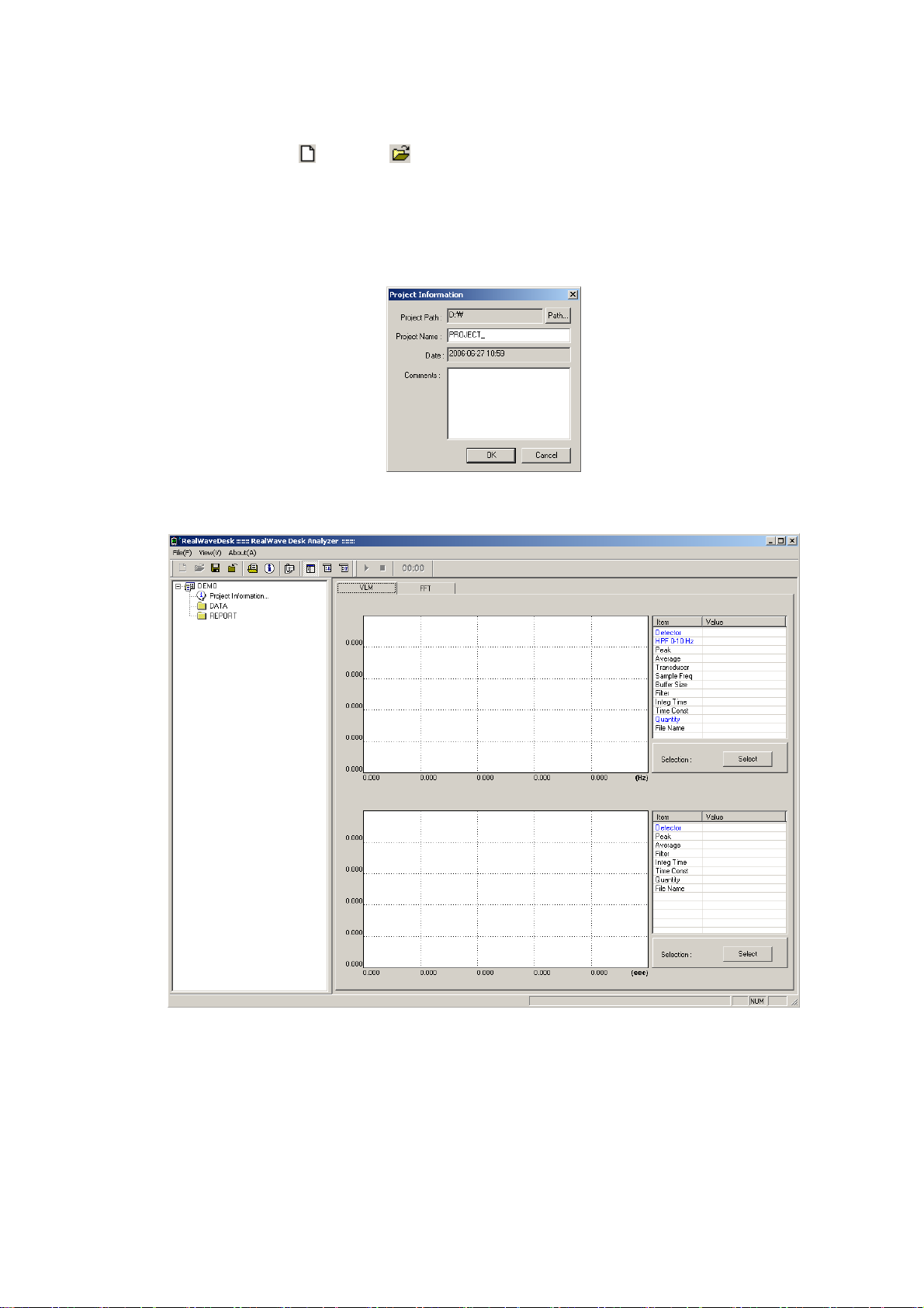
When user creates a new project of file menu, project information dialog is opened. Choose the
route of the project which has to be installed, enter the project name and just put the OK button [Fig.
VII-1-1]. After then a new project like [Fig. VII-1-2] will be created.

[Fig. VII-1-1] Enter the information of Project

[Fig. VII-1-2] Program

When user opens a project of file menu and choose a project file (*.PRJ), the chosen project is
loading like [Fig. VII-1-3].

55

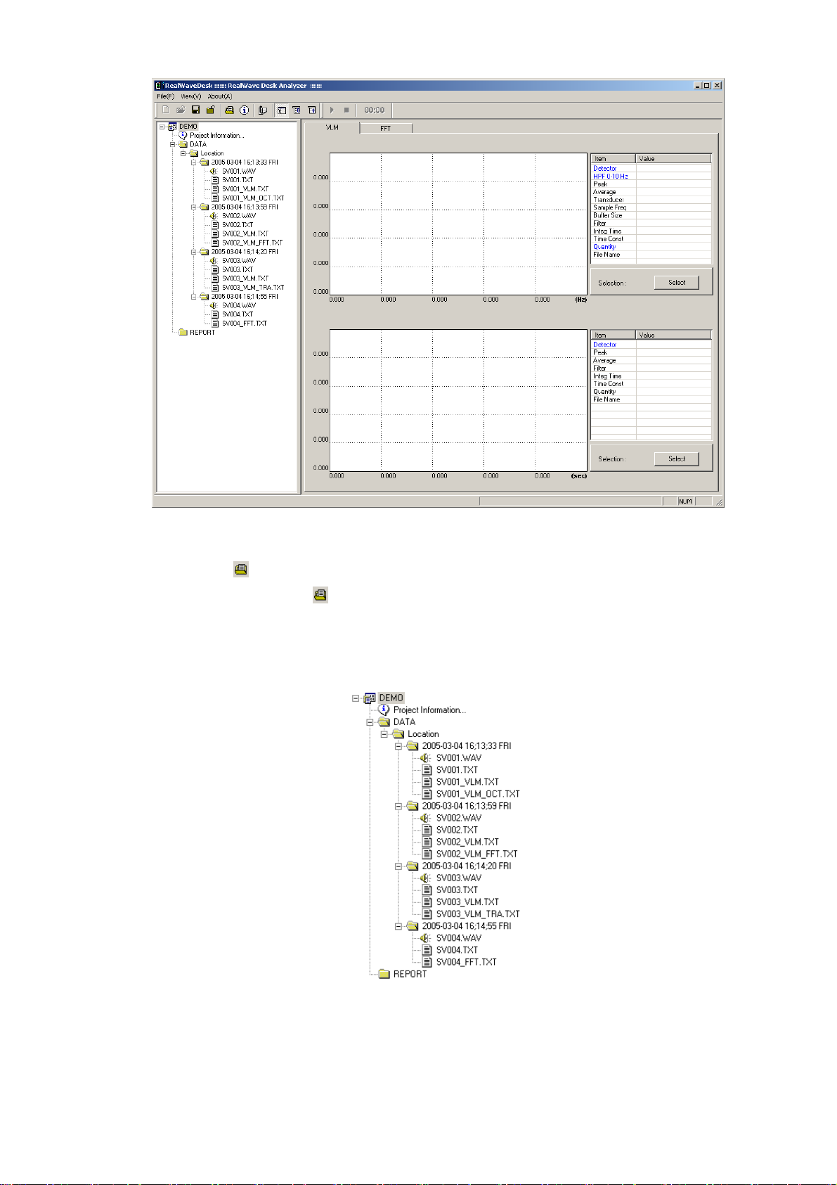
[Fig. VII-1-3] Project loading

2. Adding a file / Delete

Click a file additional icon
click the mouse on the right button when user add a wave file of file menu and choose the wave file
which has to be added at the Project, the wave file and the result file of analysis are added like [Fig.
VII-2-1]

on the toolbar or after choose data folder of the tree control, then

[Fig. VII-2-1] Project tree control

If user wants to the added file, user has to select the “Delete” menu in the menu window, which is

displayed by clicking of mouse right button. All file of folder and sub-folder will be deleted.

56

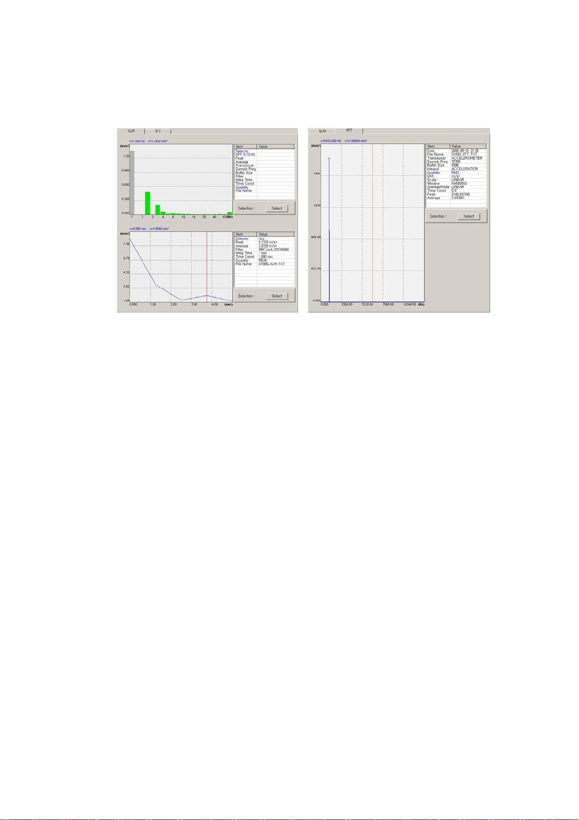
3. Control of Graph

When double clicking the folder that a data from tree control, a graph is appeared on the right of

the window like [Fig. VII-3-1].

[Fig. VII-3-1] VLM / FFT Control of Graph

• VLM Trace : The Trace graph will be displayed on the button side in VLM. User can see the
cursor value by clicking of mouse left button. Also user can select the specific range by clicking of
mouse right button and dragging

• VLM Octave : The Octave graph will be displayed on the upper side in VLM .User can see the
Octave graph corresponding to the cursor position in automatically trace graph.

• VLM FFT : The FFT graph will be displayed on the upper side in VLM peak position is detected
in the FFT graph. Also user can select the specific range by clicking of mouse right button and
dragging.

• FFT : User can display the cursor value by clicking of mouse left button, also user can select the

specific range as same way in VLM FFT.

• Selection Button : After user select the specific range in the graph control. The peak & average
values will be calculated and displayed by locking the “Select” button.

4. The Control of Property list

The property of measured data which is importanted from saved file is displayed in list control like
[Fig. VII-4-1]. Combo box will be displayed by double click of blue color character in the list, and
then user can change the parameters, displayed graph will be changed as defined parameters.

57

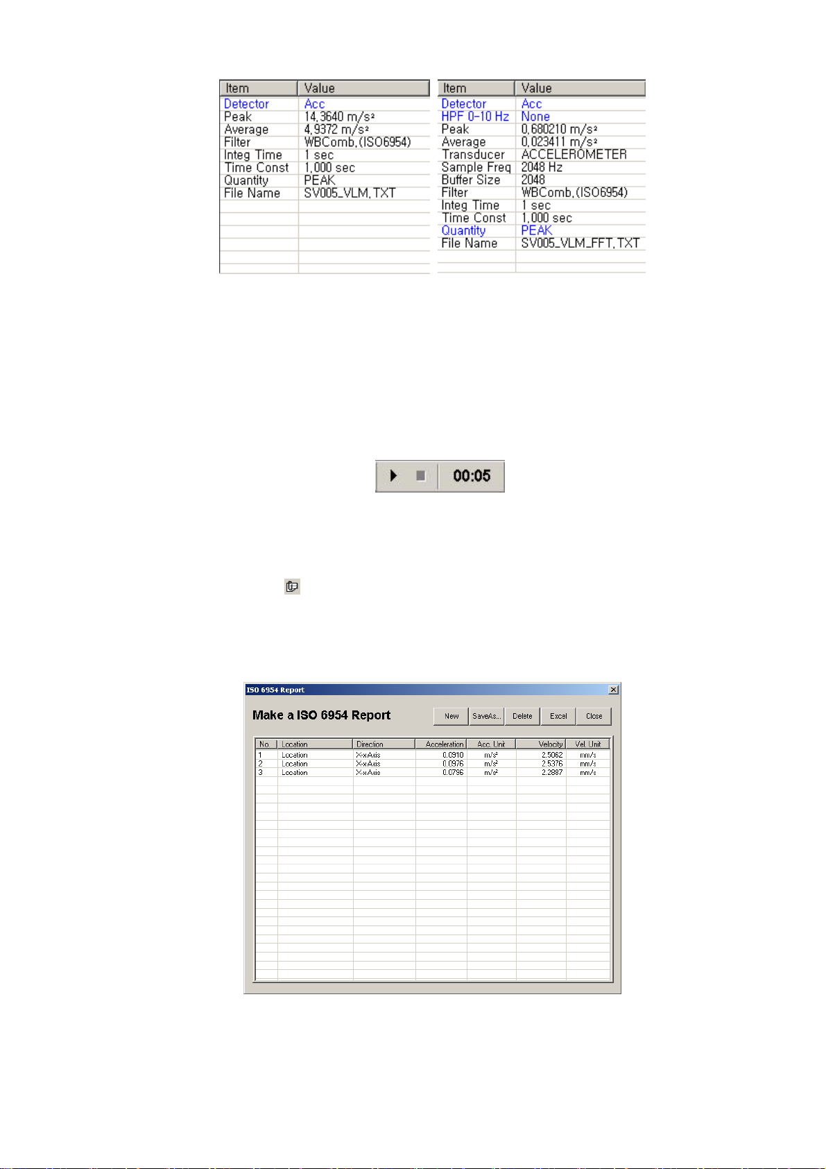
[Fig. VII-4-1] The control of property list

5. Control of Sound

If user roading the data from project tree, sound control menu of toolbar is activated like [Fig. VII-

5-1]. Sound play, stop, play time are displayed.

[Fig. VII-5-1] Control of Sound

6. List of Result Report

The measuring result data is displayed as a report form of ISO6954 like [Fig. VII-6-1] from current

project file.

[Fig. VII-6-1] Reporting of Result

• New : Tap to load a result date from current project.
58

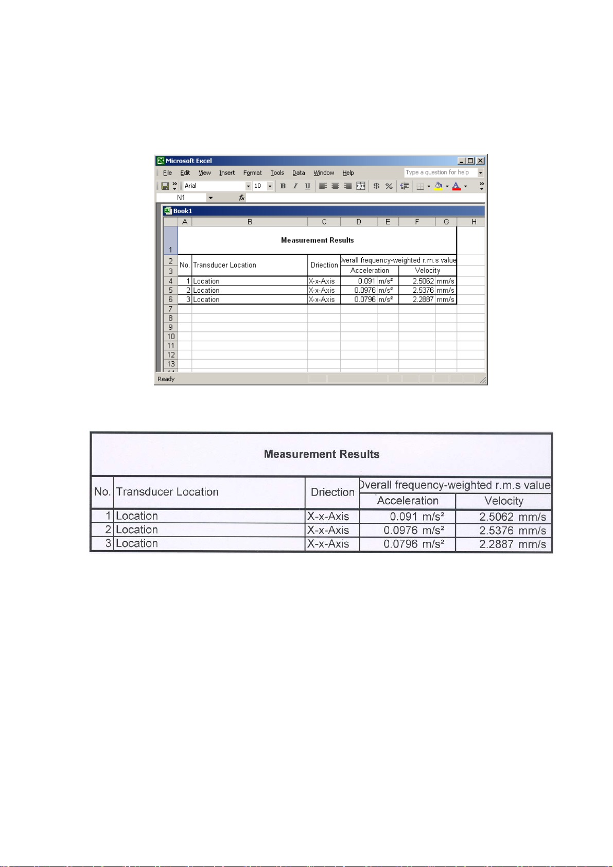
• Open : Tap to load a stored result list file.

• Save As : Tap to save a current result list file as another name.

• Delete : Tap to delete a date of selected list.

• Excel : Tap to change details of list as MS Office Excel file like [Fig. VII-6-2].

[Fig. VII-6-2] Result Report with MS Office Excel

[Fig. VII-6-3] Printed Result at MS Office Excel

59

VIII. Installation of ActiveSync and Communication with PDA

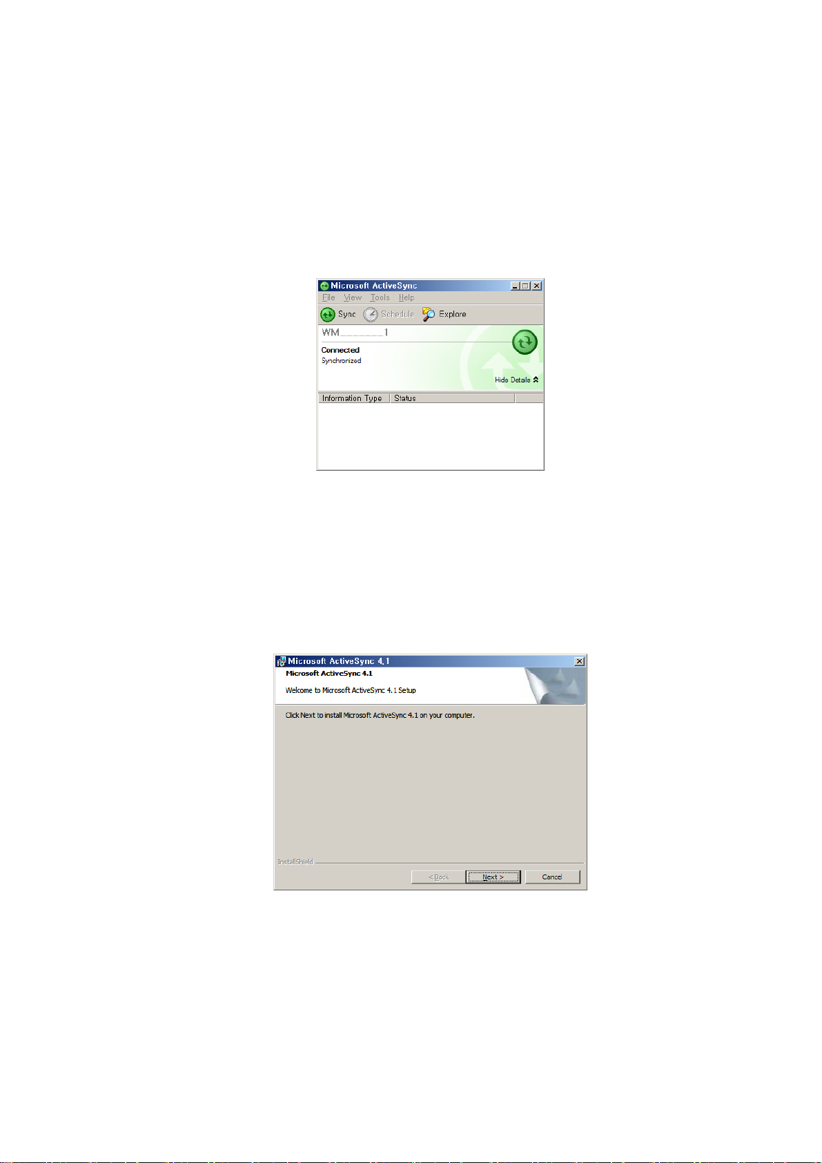
1. What is Microsoft ActiveSync?

Microsoft ActiveSync is a program which synchronizes with PC and PDA. If PDA is connected
with PC, many data is transported each other. If selecting the folder named Mobile Device, user can
see the internal data of PDA. ActiveSync program must be installed at PC which will be used before
connecting PDA at a USB port of PC.

[Fig. VIII-1-1] ActiveSync Executed W indow

2. Installation of ActiveSync

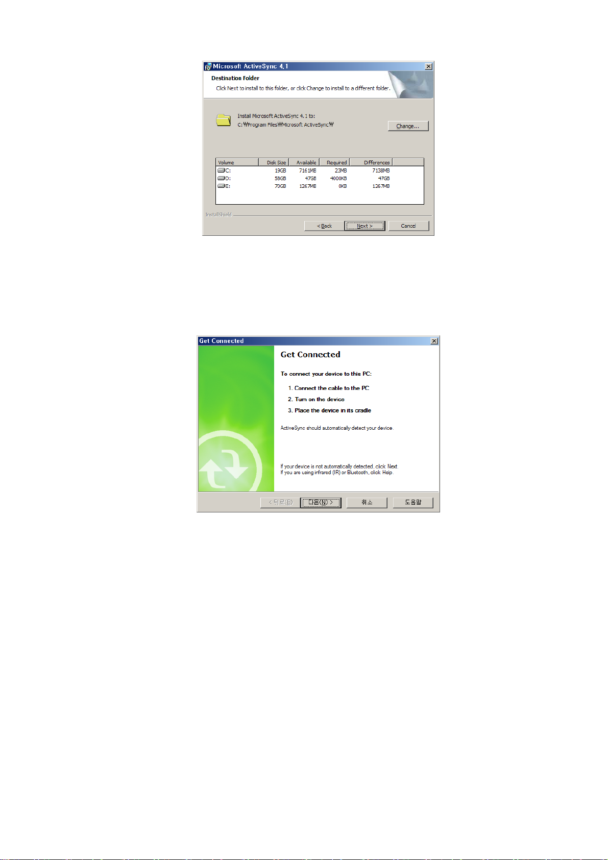
Run “MSASYNC.EXE” at the folder named “ActiveSync” in CD and follow from [Fig. VIII-2-1]
to [Fig. VIII-2-9].

[Fig. VIII-2-1]

60

[Fig. VIII-2-2]

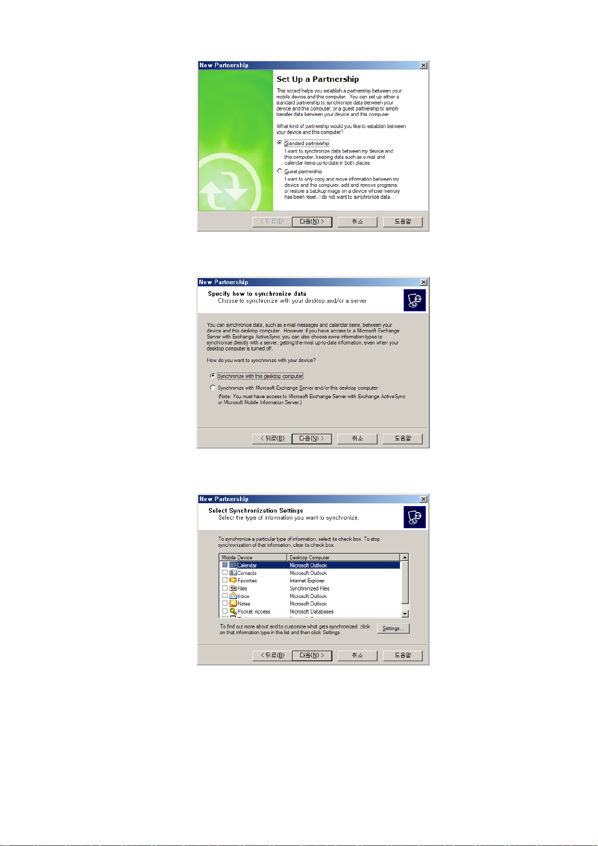
Up to here, installation of the program is completed. First, PC and PDA has to be connected eac h
other using USB cable or cradle because connection of PDA will be carried out from now on.

[Fig. VIII-2-3]

Press the NEXT button after connection as [Fig. VIII-2-3]. In the following, relationship of partner
has to be established to use PDA at the office. When standard relationship of partner is set up, Sync
item of data is selected and PDA is connected with PC, the data of PC is copied at PDA and the one
of PDA is copied at PC, so the data of each device is identical. Generally, this is called to be Sync
(Synchronization). The synchronized data is Microsoft Outlook data, E-mail and the files to be set up
synchronization. If user just set up standard relationship of partner, it is useful because the connection
is completed directly without any questions for connection.

61

[Fig. VIII-2-4]

[Fig. VIII-2-5]

[Fig. VIII-2-6]

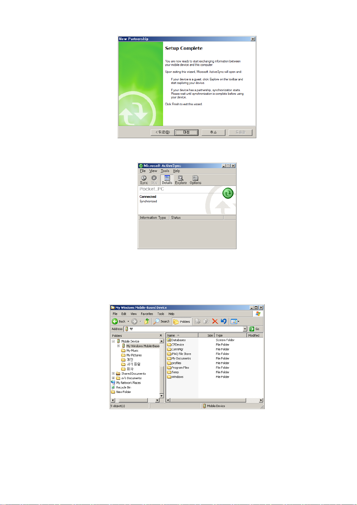
All check boxes should be unchecked like [Fig. VIII-2-6] and push the NEXT button because this
step is for what the data of PC and PDA is transferred each other. And then, the connection comes to
an end. Generally, it is not used for office but for measurement, so it is useful to delete the item of
data synchronization.

62

[Fig. VIII-2-7]

[Fig. VIII-2-8] The State of Connection

If the connection is completed, user can see and copy the entire data of PDA with the folder,
[Mobile Device] like [Fig. VIII-2-9] at Window Explorer.

[Fig. VIII-2-9] PDA Folders at Window Explorer

63

[Appendix 1]

The Theory for calculating RMS by

ISO2631 and ISO8041

64

τ

(

⎡

⎢⎥⎣

ISO8041:1990

Annex D

D. 1 Nomenclature

a : Instantaneous magnitude of signal

a : Reference magnitude of signal(

0

1/ or 1ms pW

= ) if power is measured

2

μ

: Time constant for running averaging

t : Time
t : Time of observation

o

t : Start time of integration

1

t : Stop time of integration

2

or expe : Exponential Function

()Ttt=− : Measurement period for linear averaging

21

D.2 Integration

The equivalent continuous vibration value or the equivalent continuous vibration level are based on
normal start-stop integration (linear integration) of the squared signal. The time weighting
characterizes a running integration of the squared signal. The result is the running r.m.s value.

1

t

⎡⎤

1

() ()

at atedt

rms o

=

τ

,

o

⎢⎥

∫

0

τ

⎣⎦

tt

2

2

−

o

τ

It is a function of the instant time

They are weighted by a factor decreasing exponentially with the time distance from

t . All recent parts of the signal

o

at contribute to the value.

)

t .

o

The corresponding time weighted vibration level, in decibels, is given by

tt

−

2

t

1()

at

() 10log

Lt edtdB

rms o

=

τ

,

o

∫

0

a

τ

o

⎤

τ

2

o

⎦

NOTE – These equations describe the behavior of a hot-wire ampere meter and can be realized by
relatively simple means or digital algorithms. The running r.m.s value responds to fluctuations of the
signal as slowly as the constant allows. A considerable reduction of data is achieved without losing
essential information about changes of amplitude or level.

65

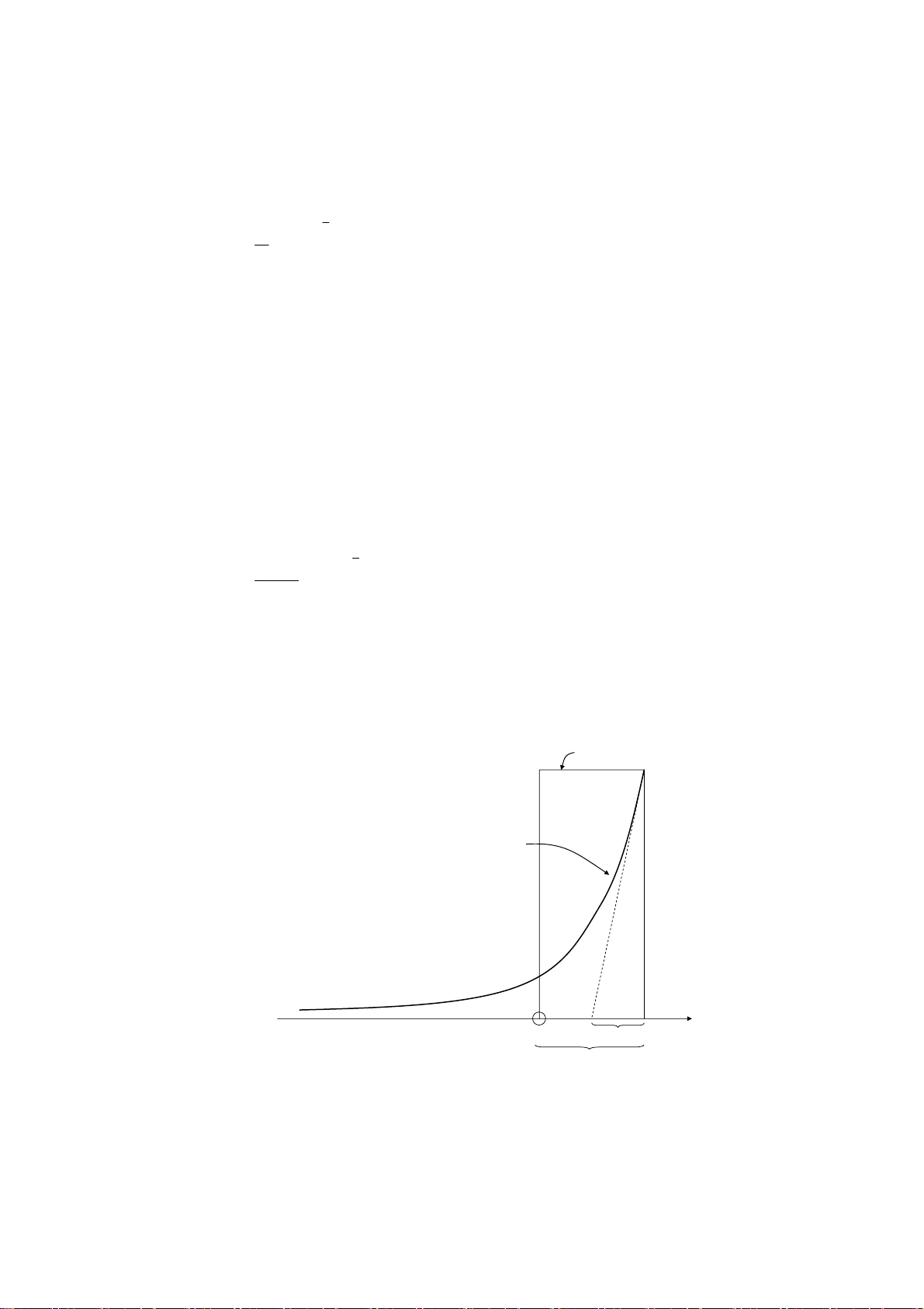
p

τ

The equivalent continuous vibration value or level can also be derived from the running level by
true integration or by summing over discrete samples,
interval

t as follows:

i

n

⎡⎤

=

aa

eq T

,0

∑

⎢⎥

i

=

⎣⎦

t

i

10

T

1

0.1

1
2

L

i

where

n

Tt

=

∑

i

=

i

1

From a statistical distribution giving the percentages
which the level is within an interval(e.g.

1dB

) around a central value Li, the equivalent value is

given by

n

⎡⎤

=

aa

eq T

,0

∑

⎢⎥

i

=

⎣⎦

100%

1

p

i

10

0.1

1
2

L

i

L being constant or nearly constant for a time

i

of the total measuring time T , during

i

where

n

p==

∑

i

1

i

100%

Linear Averaging

Exponential(τ=RC) Averaging

t

Averaging Time

t

o

[Figure] Weighting curves for linear and exponential integration

66

[Appendix 2]

Frequency Response of Filter in the

Vibration Level Meter

67

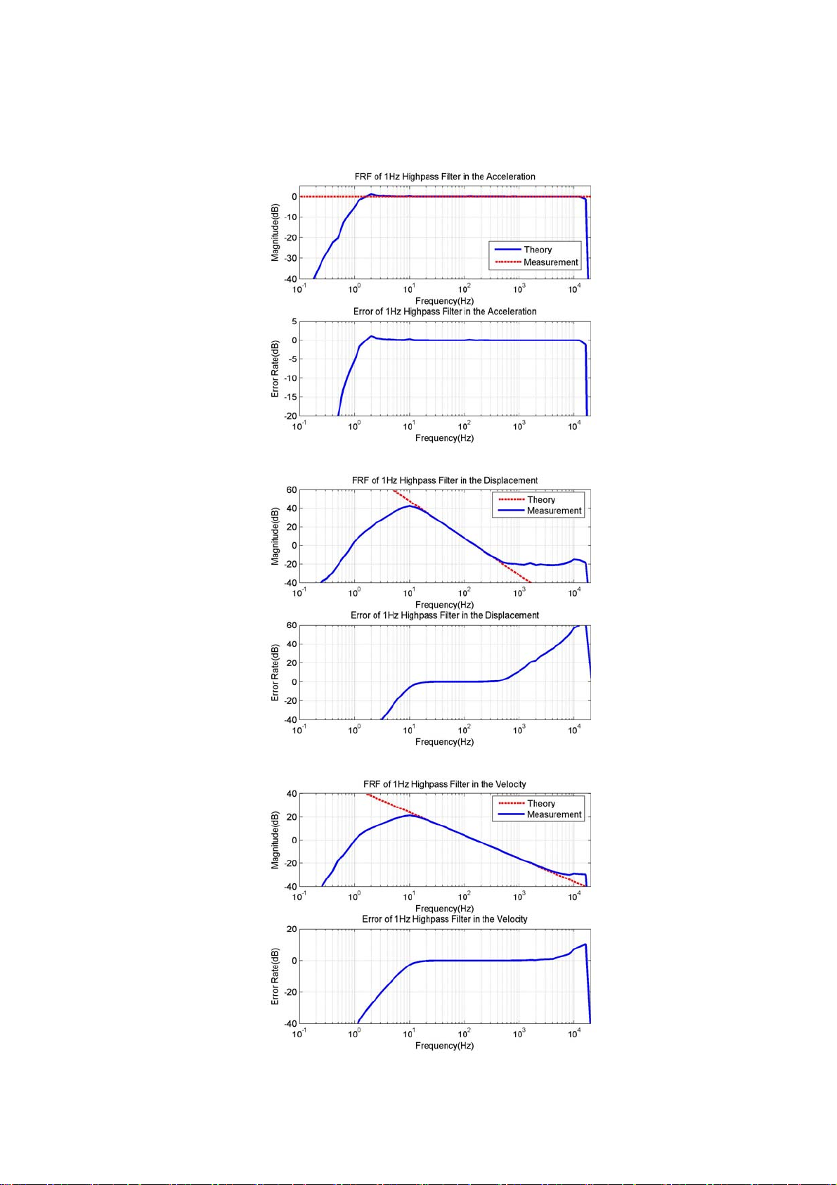
1. 1Hz Highpass Filter

A 2-pole Butterworth IIR Filter was used for this filter and integrator has highpass filter with 10Hz
Cutoff frequency.

68

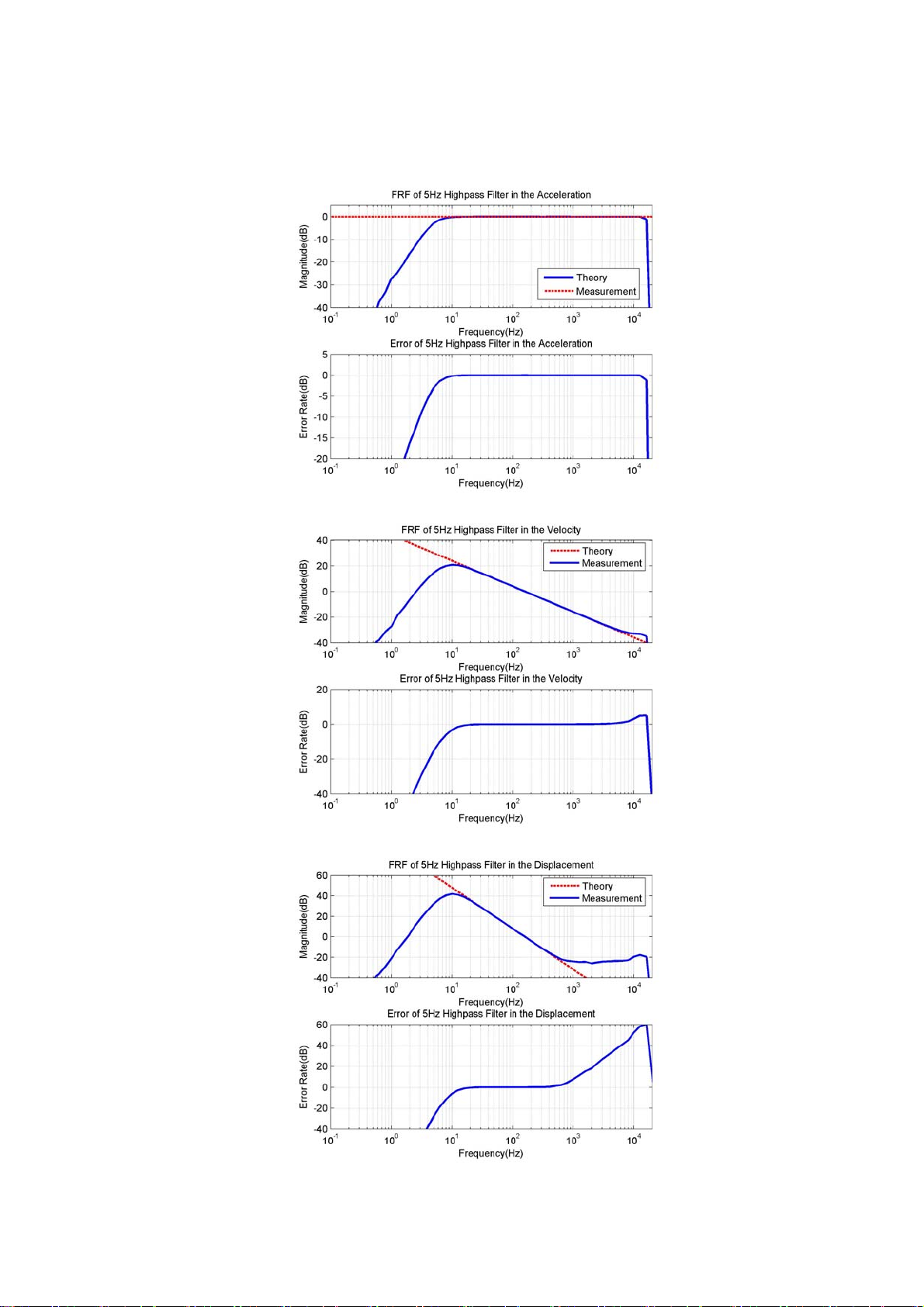
2. 5Hz Highpass Filter

A 2-pole Butterworth IIR Filter was used for this filter and integrator has highpass filter with 10Hz
Cutoff frequency.

69

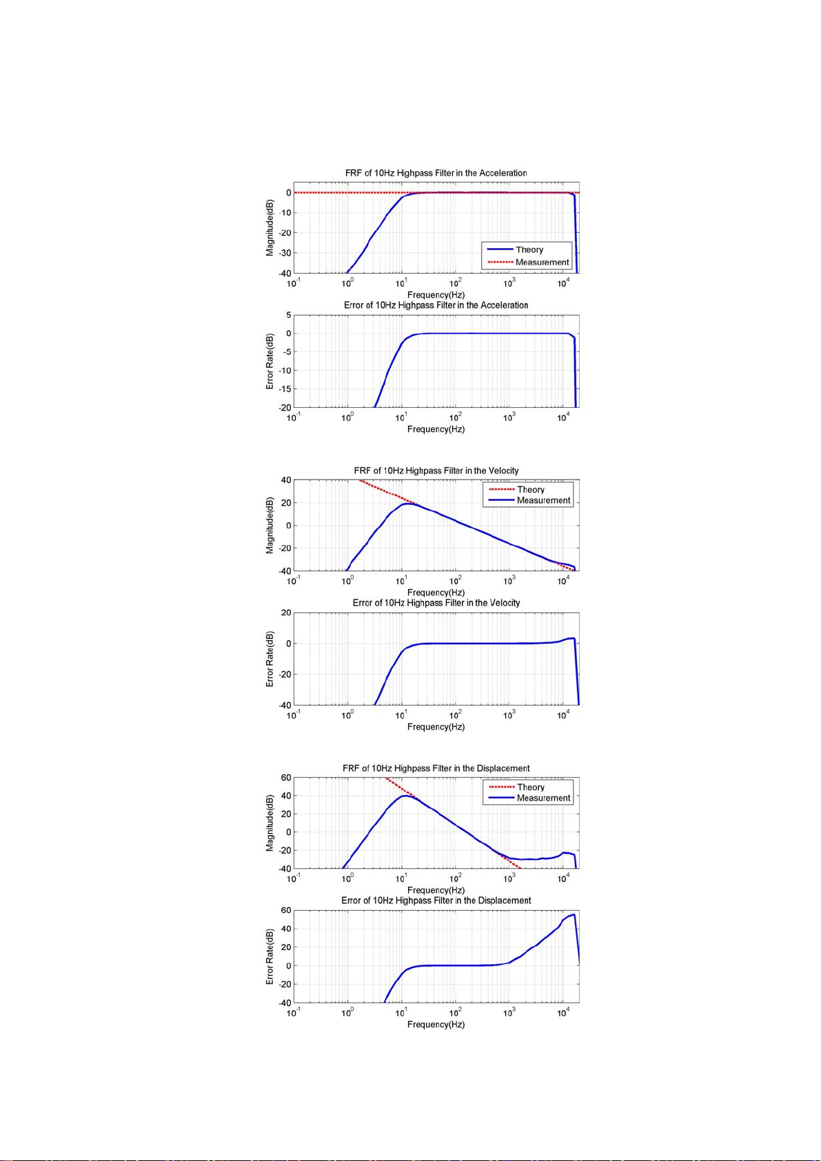
3. 10Hz Highpass Filter

A 2-pole Butterworth IIR Filter was used for this filter and integrator has highpass filter with 10Hz
Cutoff frequency.

70

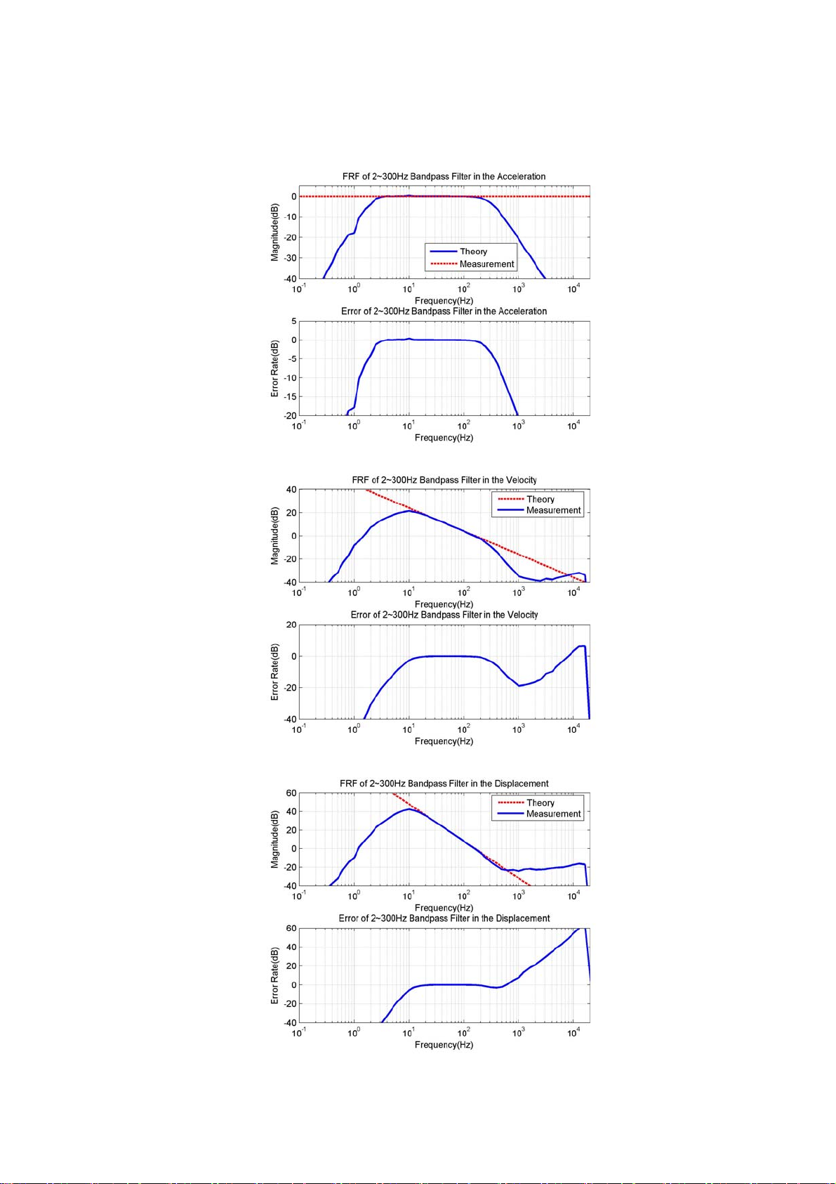
4. 2Hz~300Hz Bandpass Filter

A 4-pole Butterworth IIR Filter was used for this filter and integrator has highpass filter with 10Hz
Cutoff frequency.

71

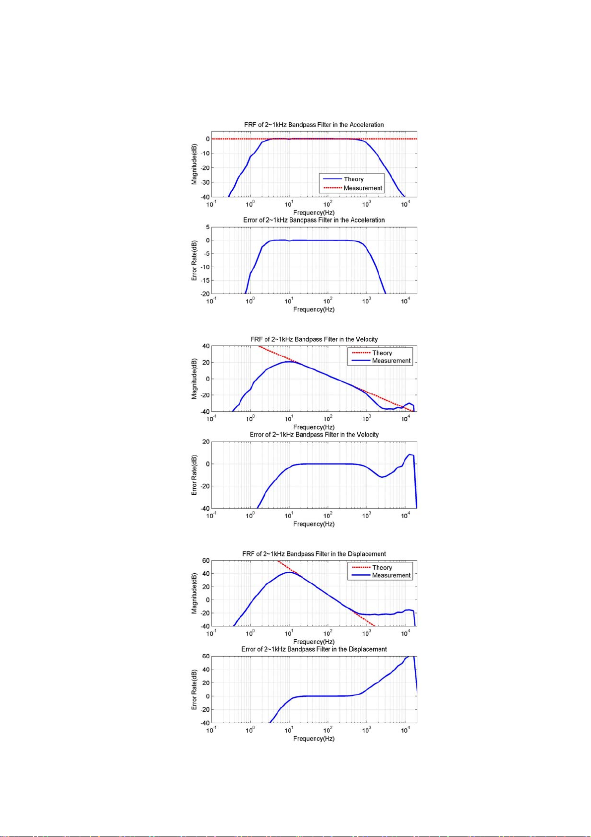
5. 2Hz~1kHz Bandpass Filter

A 4-pole Butterworth IIR Filter was used for this filter and integrator has highpass filter with 10Hz
Cutoff frequency.

72

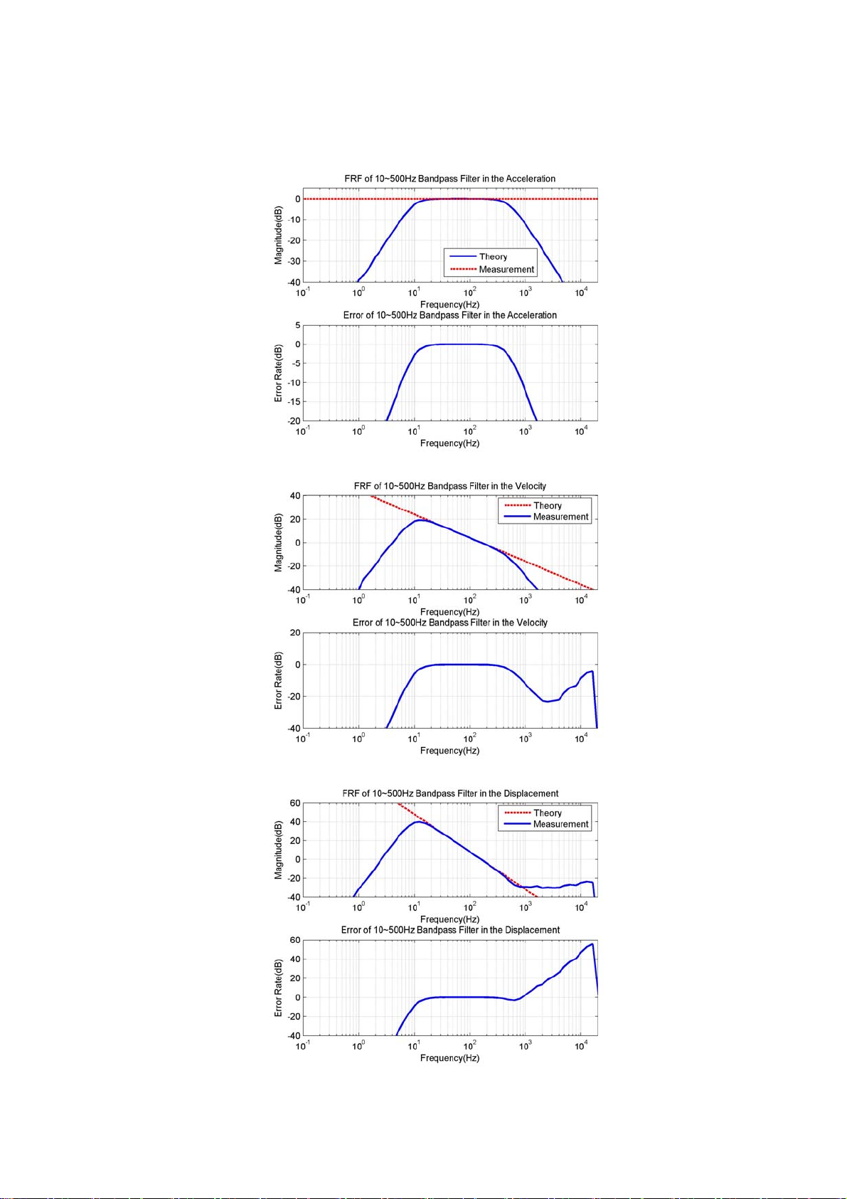
6. 10Hz~500Hz Bandpass Filter

A 4-pole Butterworth IIR Filter was used for this filter and integrator has highpass filter with 10Hz
Cutoff frequency.

73

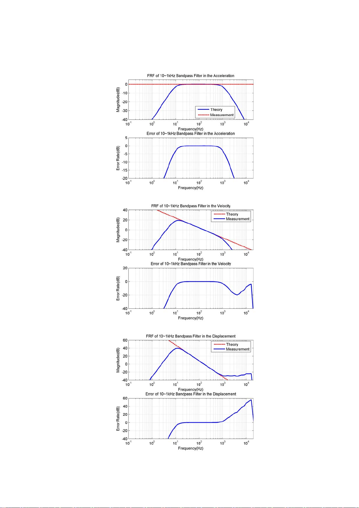
7. 10Hz~1kHz Bandpass Filter

A 4-pole Butterworth IIR Filter was used for this filter and integrator has highpass filter with 10Hz
Cutoff frequency.

74

[Appendix 3]

Theory of WBCombined Filter and

Frequency Response

(ISO6954 Filter)

75

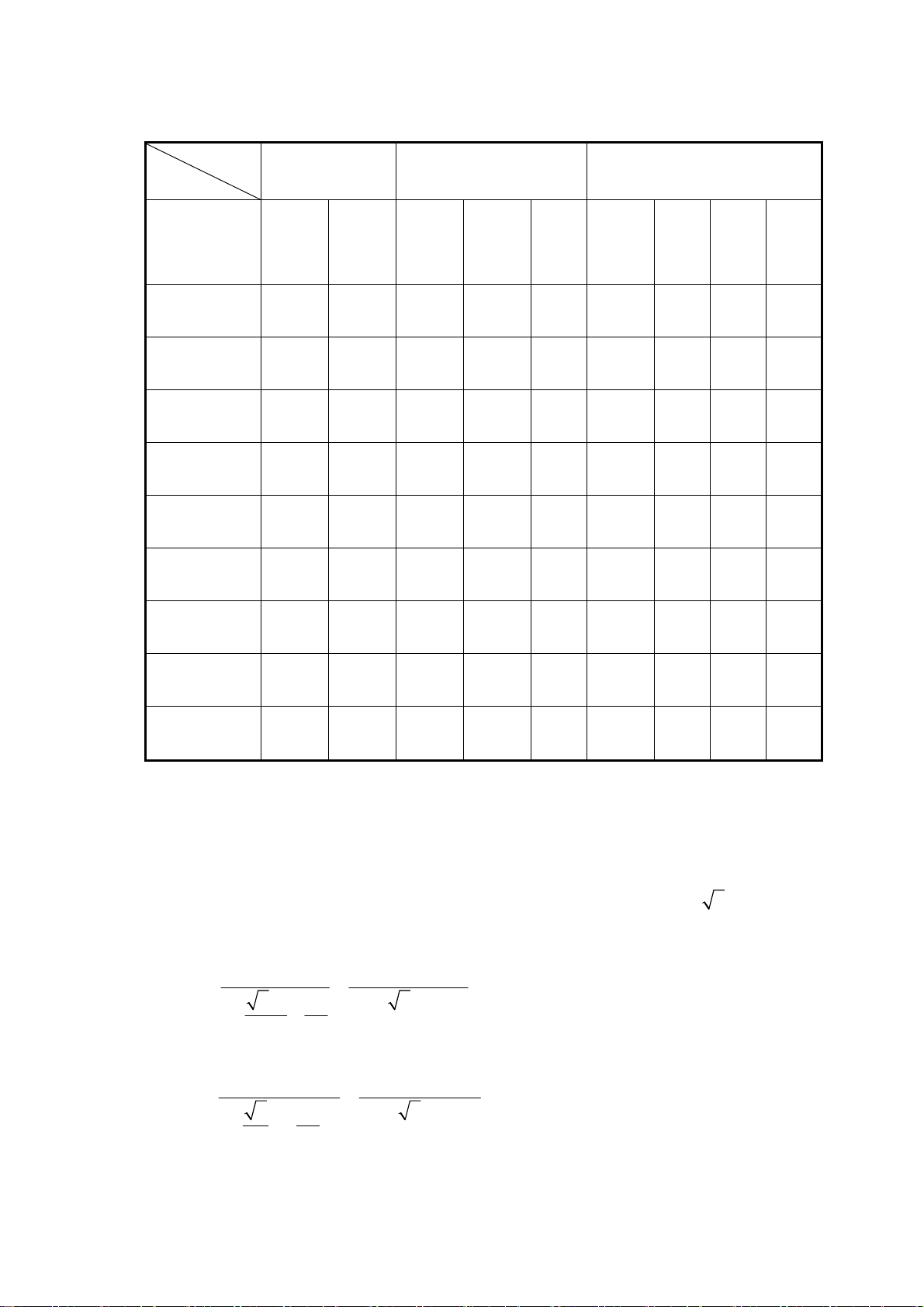
f

f

f

f

f

f

∞

f

∞

∞

∞

∞

j

∞ ∞

∞

f

f

+

1. Theory

<Table 1. Parameters of the transfer functions of frequency weightings >

Band-limiting

Weighting

1

Hz

W

k

W

d

W

WBCombined 0.7943 100 - 5.684 -

W

c

W

e

0.4 100 12.5 12.5 0.63 2.37 0.91 3.35 0.91

0.4 100 2.0 2.0 0.63

0.08 0.63

0.4 100 8.0 8.0 0.63

0.4 100 1.0 1.0 0.63

2

Hz

Acceleration-velocity

transition

3

Hz

4

Hz

0.25 0.86 0.0625 0.80 0.1 0.80

Q

4

5

Hz

Upward step

Q

5

-

-

-

-

Hz

∞

∞

∞

∞

6

Q

6

-

-

-

-

W

W

W

b

0.4 100

h

6.310 1258.9 15.915 15.915 0.64

0.4 100 16 16 0.55 2.5 0.9 4.0 0.95

- 3.75 0.91 5.32 0.91

-

∞

-

The frequencies

to

1

and the resonant quality factors

6

Q to 6Q are parameters of the

4

transfer functions determining the overall frequency weighting, referred to acceleration as input
quantity. The transfer function is expressed as a product of several factors.

a) Band-limiting(Two-pole filter with Butterworth characteristics,

12

1/ 2QQ== )

High-pass :

2

s

++

ss

Hs

()

h

==

1

1

22

ωω ω ω

++

ss

22 2

11 1 1

2

Low-pass :

2

Hs

()

l

==

++

1

1

21 2

ss

ωω

22

2

ωω

2

ω

22

2

22

ss

+

b) a-v transition(proportionality to acceleration at lower frequencies, proportionality to velocity at
higher frequencies)

76

ω

ω

+

ω

f

f

(

(

=

f

p

1

1

Hs

For W.B.Combined this expression is replaced by

()

t

=

11

1

++

Q

44 4

s

+

ω

3

ss

ωω

2

2

Hs

()

t

c) Upward step(steepness approximately 6dB per octave, proportionality to jerk)

Hs

()

s

Where

21 to 6

ωπ

==

nn

==

The product

1

==

1

s

+

1

ω

4

2

⎛⎞

ωωω

5555 5

=⋅ =

⎜⎟

ω

6

⎝⎠

fn

()

(imaginary angular frequency) 2sj jf

HsHs⋅ represents the band-limiting transfer function. Its corner

4

s

+

ω

4

11

1

++ ++

ss ss

QQ

11

1

++

() ()

hl

ss

ωω

Q

66 6

22 2

2

2

ω

2

ω

5

5

ω

22

6

+

Q

π

ss

6

6

frequencies(intersection of asymptotes) are given by

The product

certain application.

W , dW , eW , hW and W.B.Combined. This is indicated by infinity frequencies and absence of

c

quality factors in Table 1.

The total weighting function is

Hs HsHsHsHs= ⋅⋅⋅

() () () ()()

The weighting curves in annex C show the modulus(magnitude)

in a double-logarithmic scale.

NOTE 1. If the equations are interpreted in the time domain, the imaginary angular frequency

HsHs⋅ represents the actual frequency weighting transfer function for a

)()

ts

()

t

1

Hs= for frequency weighting

hlts

and

1

W ;

j

.

2

Hs

s

1

for frequency weighting

)

H of H versus the frequency

77

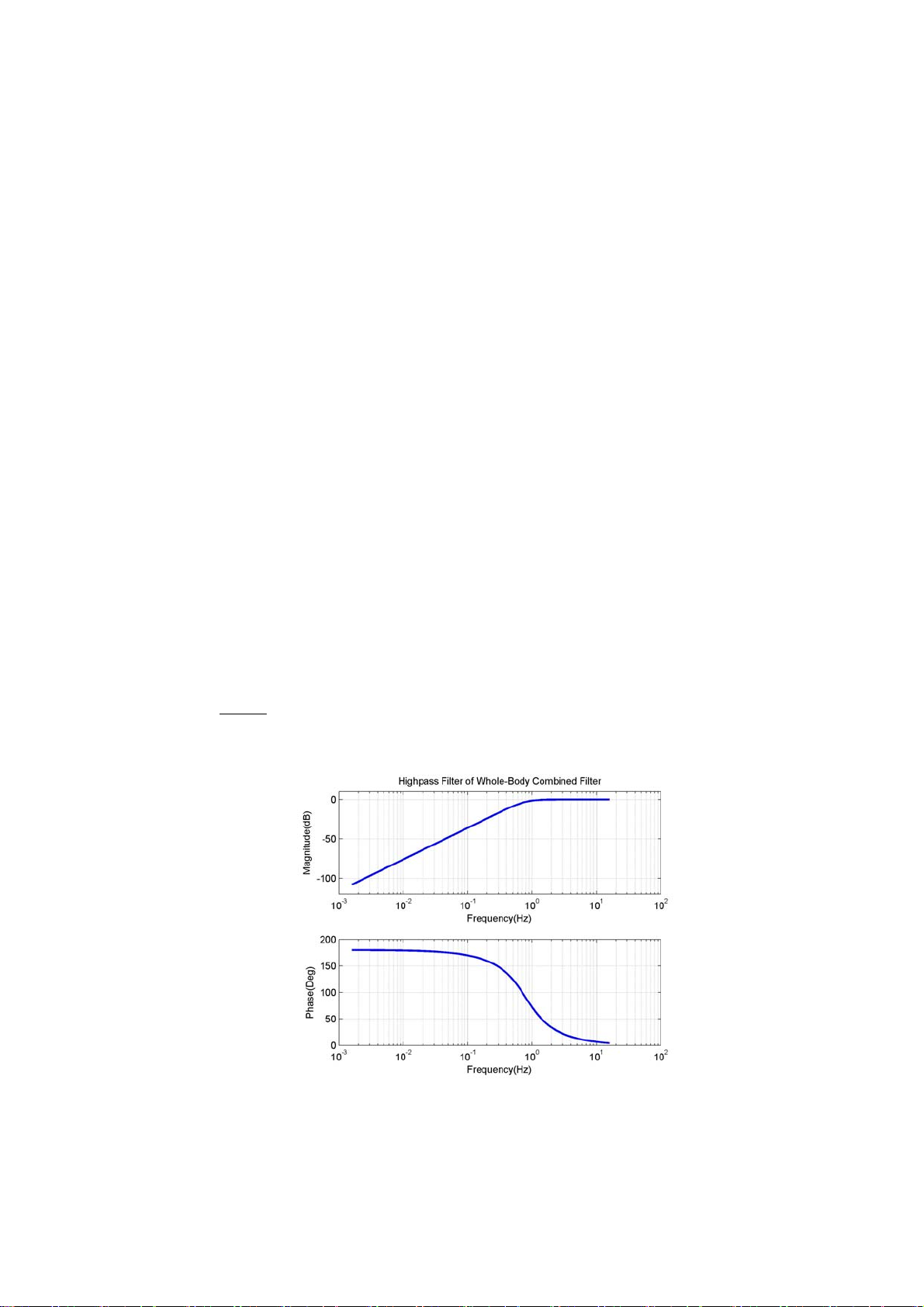
Δ

z

(

f

f

=

f

=

=

=

leads directly to the differential operator

dt

, which may be approximated by tΔ in a digital

realization of the weighting if the sampling interval

t

is small enough.

NOTE 2. Frequency weighting
direction comfort in rail vehicles.

Hs HsHsHsHs=⋅⋅⋅⋅

1.024

() () ()()

hlts

Where the parameter values

()

Hp are :

s

1

5

0.4fHz= ;

2.5fHz= ;

2

5

100fHz

0.9Q

;

W is considered to be the appropriate weighting curve for

b

W is defined in BS6841:1987, and is equivalent to :

b

)

;

34

4.0fHz= ;

6

to

1

fHz== ;

6

16

and

Q to 6Q for ()

4

0.55Q

4

0.95Q

6

;

Hp, ()

h

Hp, ()

l

Hp and

t

NOTE 3. Parameter values in [Table 1] define exactly the frequency weighting

W , eW and iW according to ISO2631-1:1997.

c

W , dW , tW ,

k

NOTE 4. Frequency weighting W.B.Combined and

W ,(formerly H.A) are unchanged by this

h

amendment. The parameter values in Table 1 are chosen to reproduce the weighting curves of ISO
8041:1990 using formulae of ISO2631:1997.

Above analog frequency response function is transferred to digital frequency response function by
bilinear transformation method which is below :

1

−

⎛⎞

−

1

=

sF

2

z

⎜⎟

s

+

1

⎝⎠

1

−

z

<Fig. 1 Highpass Filter with 0.7943Hz Cutoff>

78

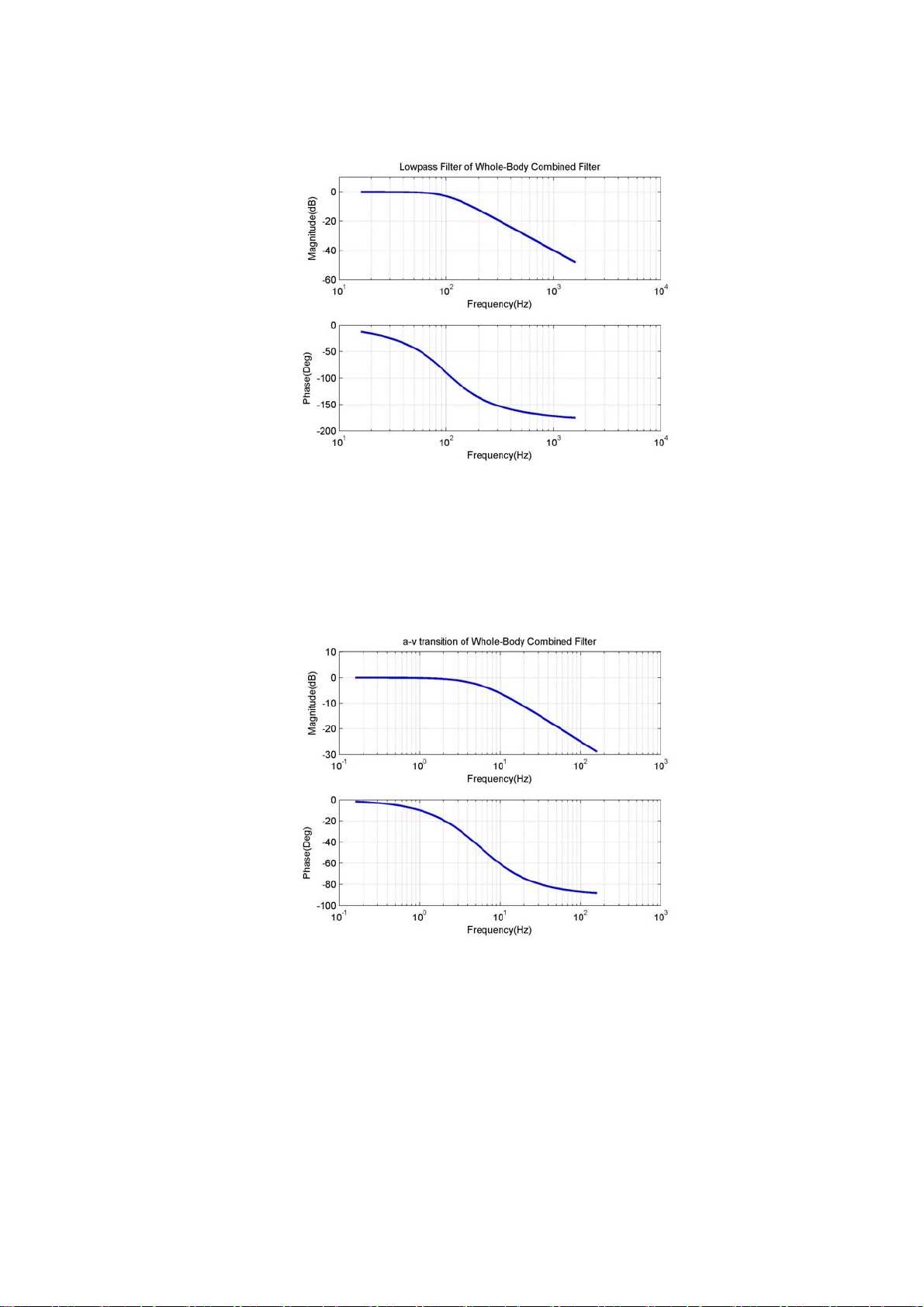
<Fig. 2 Lowpass Filter with 100Hz Cutoff>

<Fig. 3 a-v transition Frequency Response>

79

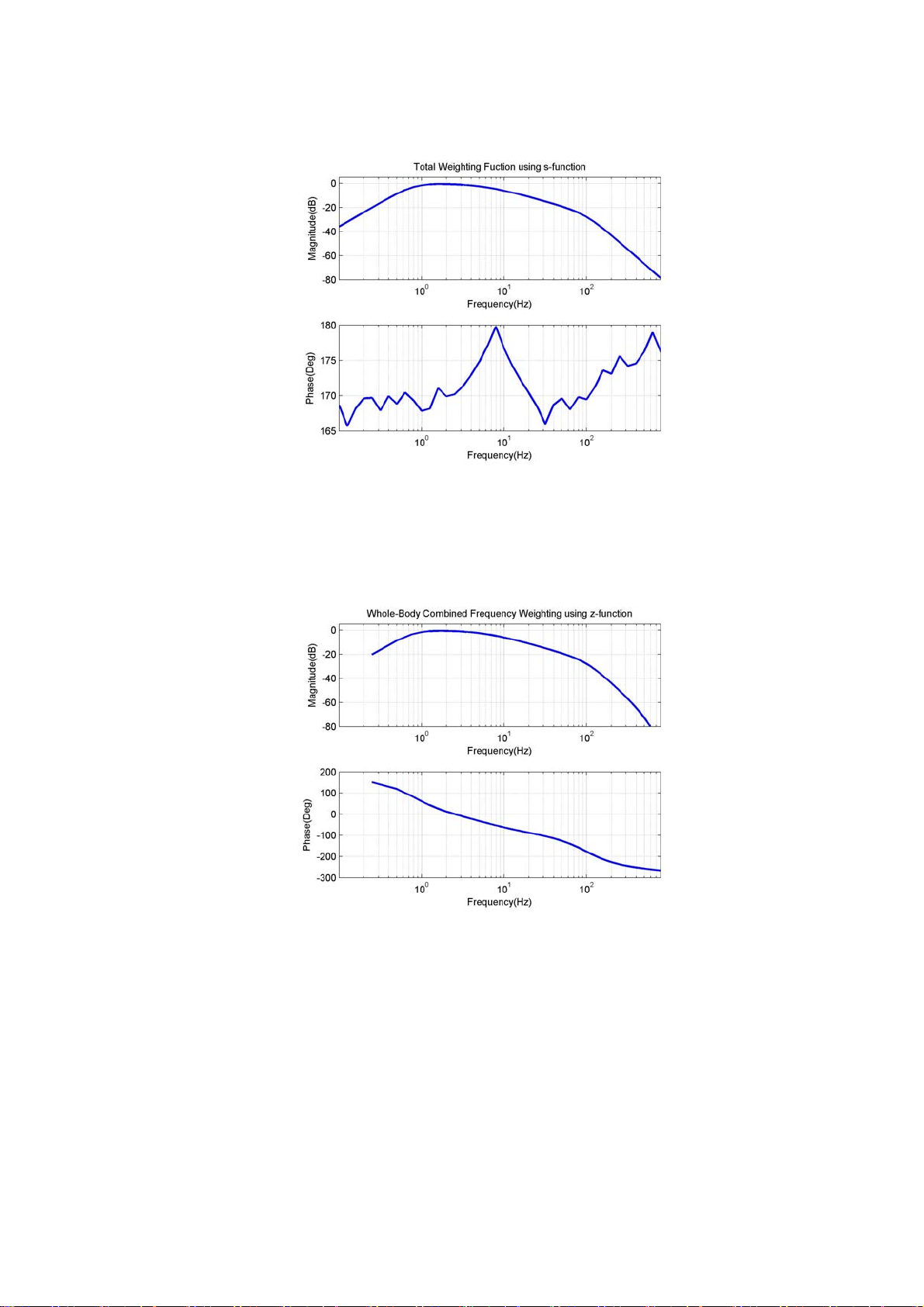
<Fig. 4 Frequency Response of Whole-body Combined Filter using s-function>

<Fig. 5 Frequency Response of Whole-body Combined Filter using z-function>

80

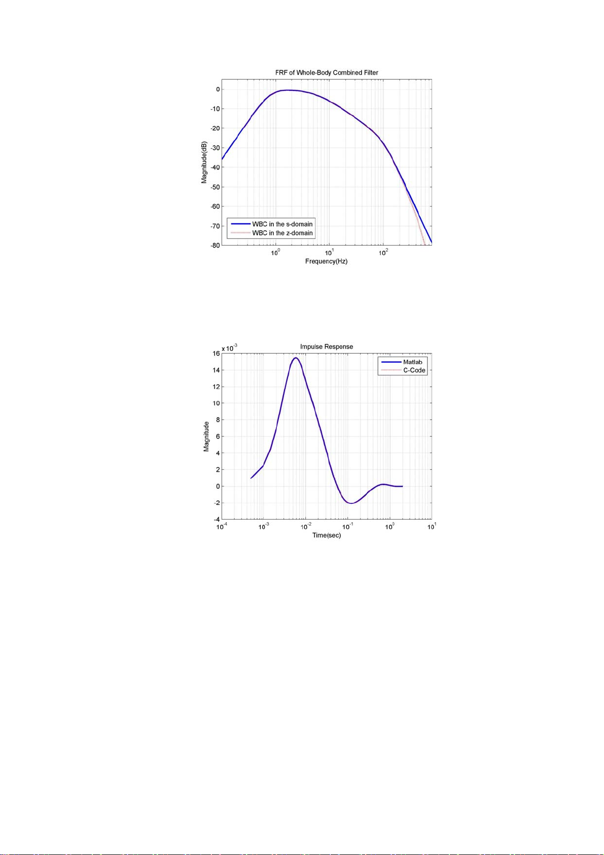
<Fig. 6 Comparison of Whole-body Combined Filter>

<Fig. 7 Impulse Response Function in the Matlab and C-code>

A simulated impulse response function is same to a theoretical impulse response function in C­code’s algorithms as shown in [Fig. 7]. Where the sampling frequency for simulation is
2048Sample/sec, a buffer size is 4096.

81

<Table 2. Error between Standard and Calculated Filter>

Frequency WBCombined(dB)

Nominal TRUE Calculated Standard

0.100 0.1 -36.002 -36 0.005555

0.125 0.12589 -32.004 -32 0.012498

0.160 0.15849 -28.01 -28.01 0

0.200 0.19953 -24.022 -24.02 0.008326

0.250 0.25119 -20.051 -20.05 0.004987

0.315 0.31623 -16.121 -16.12 0.006203

0.400 0.39811 -12.286 -12.29 -0.03256

0.500 0.50119 -8.672 -8.67 0.023063

0.630 0.63096 -5.5082 -5.5 0.148869

0.800 0.79433 -3.094 -3.09 0.129282

1.000 1 -1.5876 -1.59 -0.15117

1.250 1.2589 -0.84682 -0.85 -0.37552

1.600 1.5849 -0.59086 -0.59 0.145551

2.000 1.9953 -0.61239 -0.61 0.390274

2.500 2.5119 -0.81796 -0.82 -0.2494

3.150 3.1623 -1.1884 -1.19 -0.13463

4.000 3.9811 -1.7404 -1.74 0.022983

5.000 5.0119 -2.5008 -2.5 0.03199

6.300 6.3096 -3.4885 -3.49 -0.043

8.000 7.9433 -4.7032 -4.7 0.068039

10.000 10 -6.1234 -6.12 0.055525

12.500 12.589 -7.7138 -7.71 0.049262

16.000 15.849 -9.4352 -9.44 -0.05087

20.000 19.953 -11.253 -11.25 0.02666

25.000 25.119 -13.141 -13.14 0.00761

31.500 31.623 -15.088 -15.09 -0.01326

40.000 39.811 -17.102 -17.1 0.011695

50.000 50.119 -19.228 -19.23 -0.0104

63.000 63.096 -21.581 -21.58 0.004634

80.000 79.433 -24.385 -24.38 0.020504

100.000 100 -27.931 -27.93 0.00358

125.000 125.89 -32.371 -32.37 0.003089

160.000 158.49 -37.551 -37.55 0.002663

200.000 199.53 -43.176 -43.18 -0.00926

250.000 251.19 -49.017 -49.02 -0.00612

315.000 316.23 -54.952 -54.95 0.00364

400.000 398.11 -60.925 -60.92 0.008207

500.000 501.19 -66.914 -66.91 0.005978

630.000 630.96 -72.91 -72.91 0

800.000 794.33 -78.908 -78.91 -0.00253

Error(%)

82

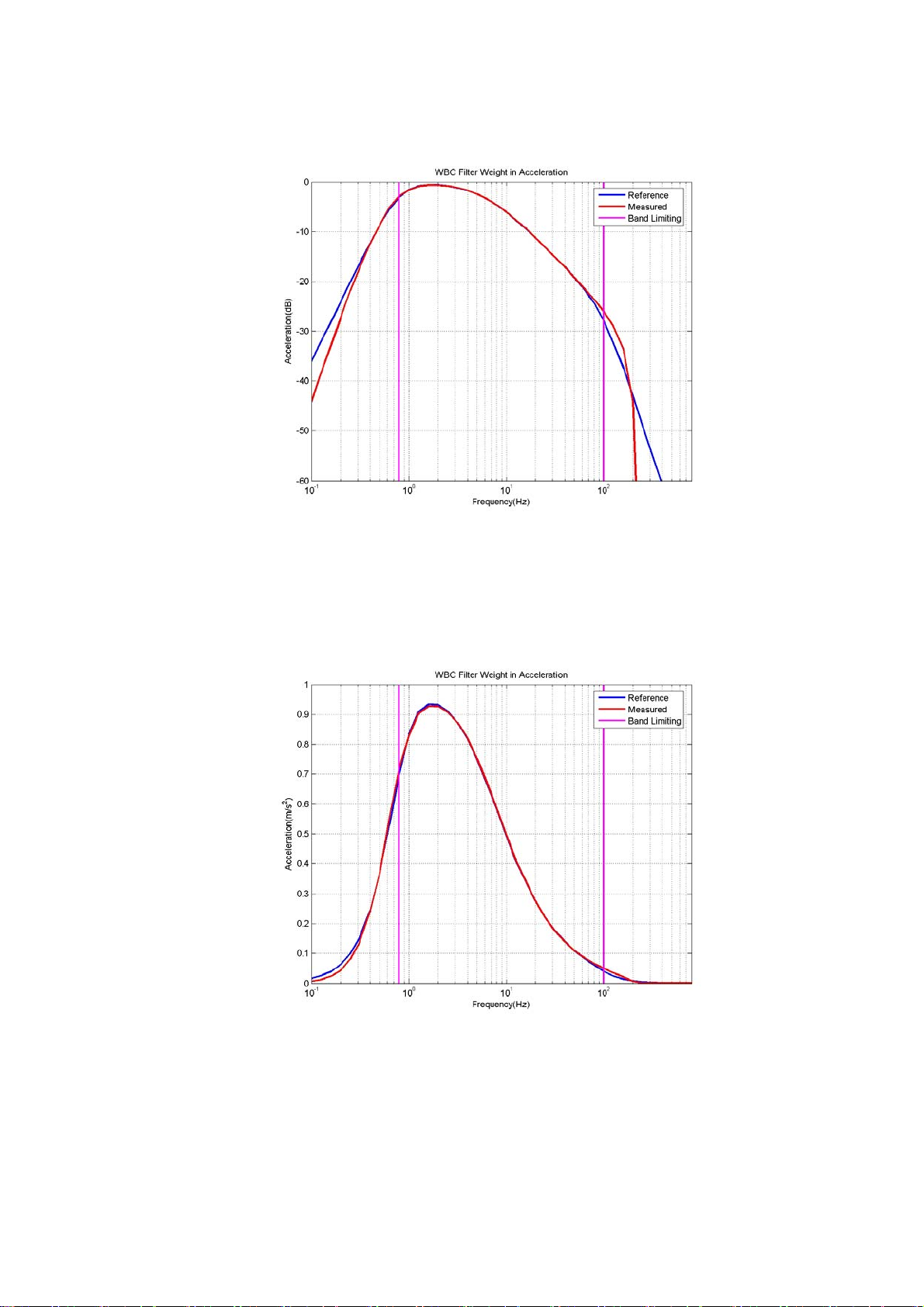
2. Frequency Response and weight factor of Weighting Filter as acceleration input

<Fig. 8 Comparison of a theoretical acceleration and a measured acceleration (y-axis : Decibel)>

<Fig. 9 Comparison of a theoretical acceleration and a measured acceleration (y-axis : Linear)>

83

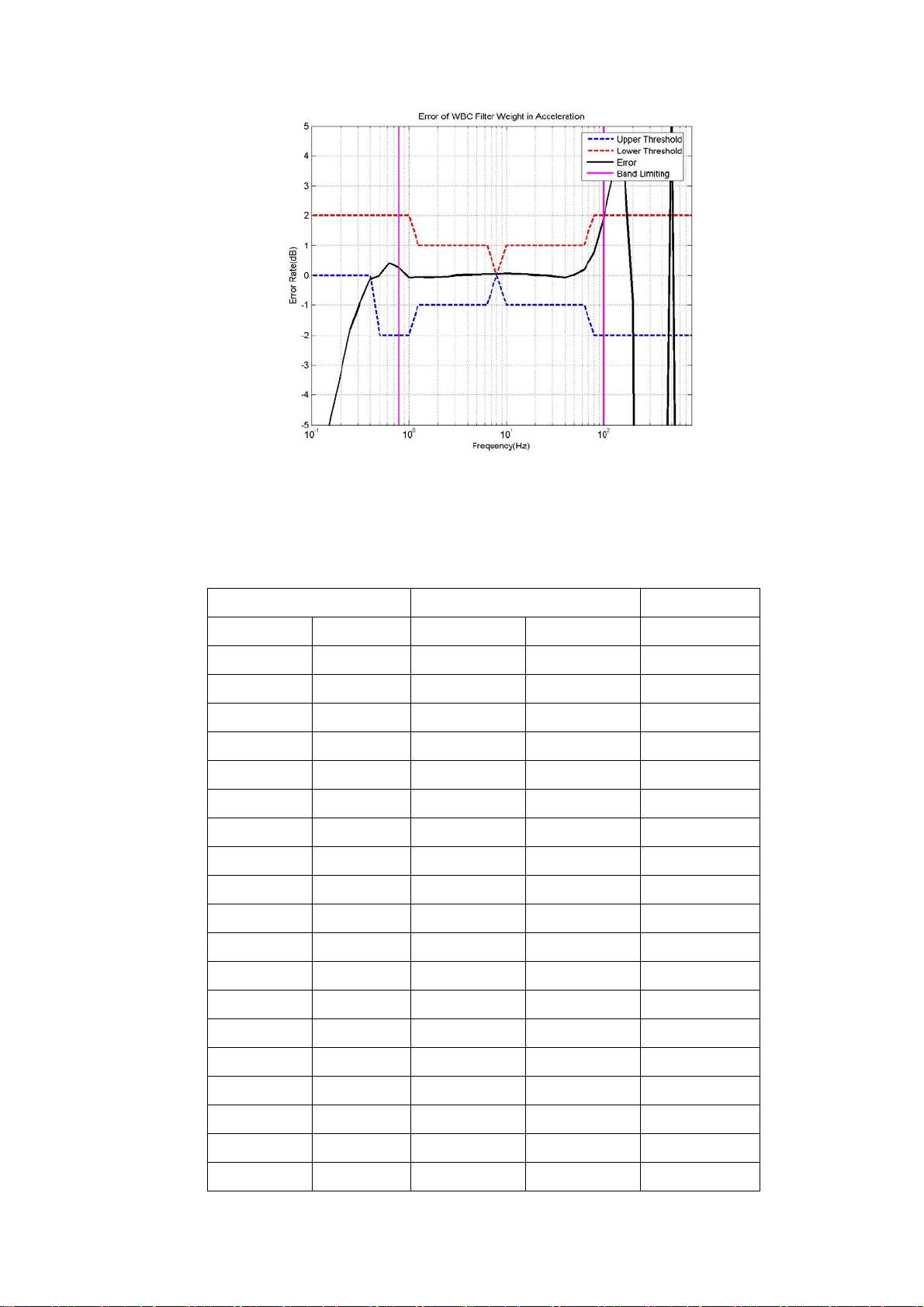
<Fig. 10 Error Range and Acceleration’s Error >

Error curve is in a upper and lower threshold line within band limiting frequencies.

<Table 3. Combined frequency weighting, defined from 1Hz to 80Hz, in one-third-octave bands>

Frequency WBCombined Weight Tolerance

TRUE Nominal Factor Wm dB dB

0.1000 0.100 0.015800 -36.03 + 2

0.1259 0.125 0.025100 -32.01 + 2

0.1585 0.160 0.040000 -27.96 + 2

0.1995 0.200 0.062900 -24.03 + 2

0.2512 0.250 0.099400 -20.05 + 2

0.3162 0.315 0.156000 -16.14 + 2

0.3981 0.400 0.243000 -12.29 + 2

0.5012 0.500 0.368000 -8.68 ± 2

0.6310 0.630 0.530000 -5.51 ± 2

0.7943 0.800 0.700000 -3.10 ± 2

1.0000 1.000 0.833000 -1.59 ± 2

1.2590 1.250 0.907000 -0.85 ± 1

1.5850 1.600 0.934000 -0.59 ± 1

1.9950 2.000 0.932000 -0.61 ± 1

2.5120 2.500 0.910000 -0.82 ± 1

3.1620 3.150 0.872000 -1.19 ± 1

3.9810 4.000 0.818000 -1.74 ± 1

5.0120 5.000 0.750000 -2.50 ± 1

6.3100 6.300 0.669000 -3.49 ± 1

84

7.9430 8.000 0.582000 -4.70 0 0

10.0000 10.000 0.494000 -6.13 ± 1

12.5900 12.500 0.411000 -7.72 ± 1

15.8500 16.000 0.337000 -9.45 ± 1

19.9500 20.000 0.274000 -11.24 ± 1

25.1200 25.000 0.220000 -13.15 ± 1

31.6200 31.500 0.176000 -15.09 ± 1

39.8100 40.000 0.140000 -17.08 ± 1

50.1200 50.000 0.109000 -19.25 ± 1

63.1000 63.000 0.083400 -21.58 ± 1

79.4300 80.000 0.060400 -24.38 ± 2

100.0000 100.000 0.040100 -27.94 ± 2

125.9000 125.000 0.024100 -32.36 ± 2

158.5000 160.000 0.013300 -37.52 ± 2

199.5000 200.000 0.006940 -43.17 ± 2

251.2000 250.000 0.003540 -49.02 + 2

316.2000 315.000 0.001790 -54.94 + 2

398.1000 400.000 0.000899 -60.92 + 2

501.2000 500.000 0.000451 -66.92 + 2

631.0000 630.000 0.000226 -72.92 + 2

794.3000 800.000 0.000113 -78.94 + 2

85

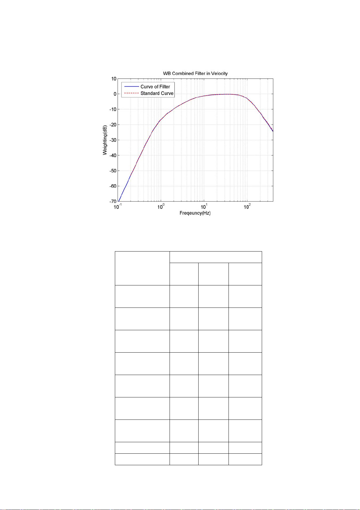
3. Frequency Response and weight factor of Weighting Filter as velocity input

<Fig. 11> Velocity W e ighting Factor

<Table 4> Velocity Weight Factor in Human Vibration

True

Frequency(Hz)

0.1995

0.2512

0.3162

0.3981

0.5012

Velocity Weighting

Referen

ce

0.0022
1

0.0043
9

0.0087
0

0.0170
0

0.0325
0

Calculat

0.00223 -0.679

0.00438 0.150

0.00868 0.260

0.01701 -0.053

0.03246 0.135

ed

Error(%)

0.6310

0.0589
0

0.0979

0.7943
0

1.000 0.147 0.147 0.313

1.259 0.201 0.201 0.040

0.05889 0.025

0.09779 0.115

86

1.585 0.260 0.261 -0.196

1.995 0.327 0.327 -0.028

2.512 0.402 0.402 -0.055

3.162 0.485 0.485 -0.035

3.981 0.573 0.573 -0.037

5.012 0.661 0.661 -0.024

6.310 0.743 0.743 0.013

7.943 0.813 0.813 -0.021

10.000 0.869 0.869 -0.036

12.590 0.911 0.911 -0.033

15.850 0.941 0.941 -0.001

19.950 0.961 0.961 0.003

25.120 0.973 0.973 -0.042

31.620 0.979 0.979 -0.035

39.810 0.978 0.978 0.026

50.120 0.964 0.964 0.037

63.100 0.925 0.925 -0.014

79.430 0.844 0.843 0.118

100.000 0.706 0.705 0.201

125.900 0.533 0.531 0.439

158.500 0.370 0.366 0.959

199.500 0.244 0.240 1.635

251.200 0.156 0.153 2.103

316.200 0.100 0.096 3.856

398.100 0.063 0.059 6.184

87

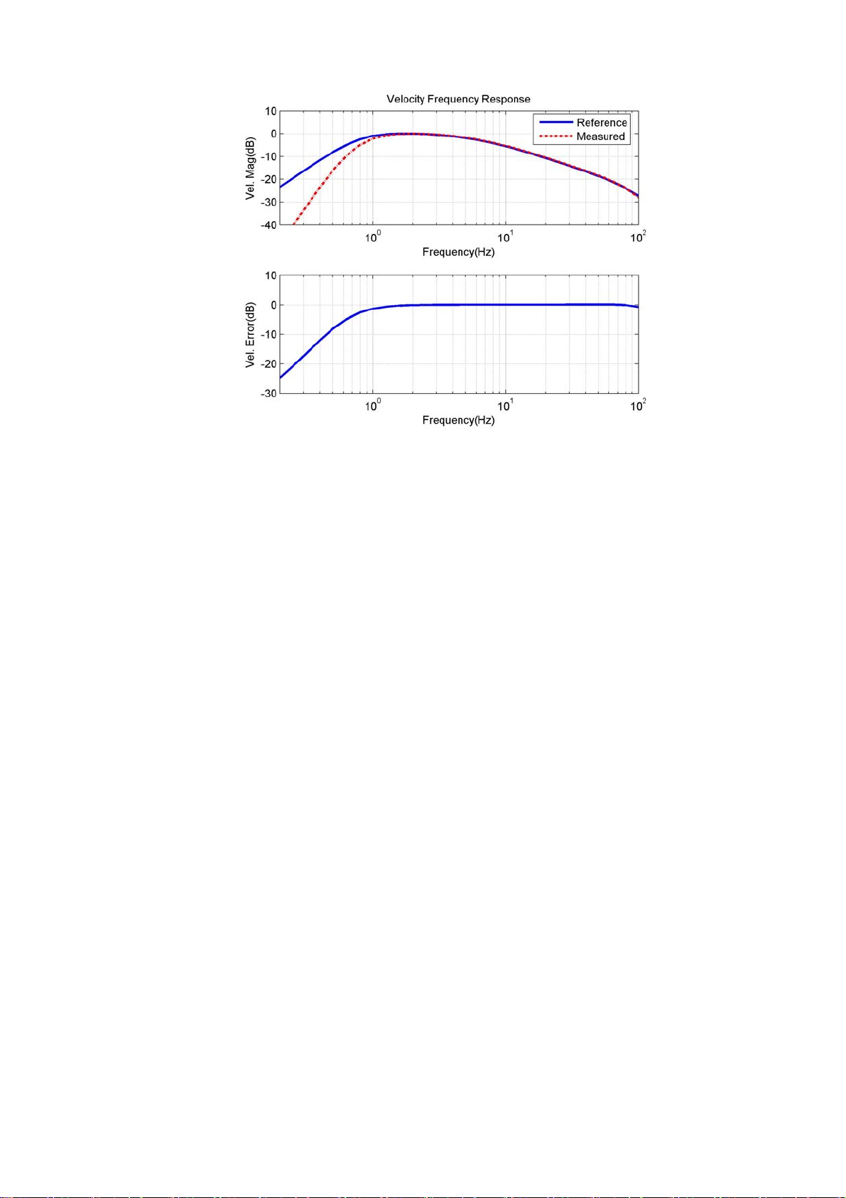
<Fig. 12> Error between theoretical value and measured value

88