Sunshine Books Machine Code Games Routines for the Commodore 64 a

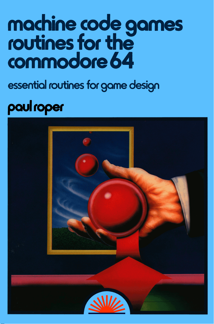
machine code gomes

routines for the

commodore 64

essential routines for game design

poulfoper

machine code gomes
routines for the
commodore 64

essential routines for gome design

paul roper

First published 1984 by:
Sunshine Books (an imprint of Scot Press Ltd.)
12-13 Little Newport Street
London WC2R 3LD

Copyright © Paul Roper, 1984
Reprinted 1984

All rights reserved. No part of this publication may be reproduced, stored
in a retrieval system, or transmitted in any form or by any means,
electronic, mechanical, photocopying, recording and/or otherwise,

without the prior written permission of the Publishers.

British Library Cataloguing in Publication Data

Roper, Paul

Machine code games routines for the Commodore 64.

1. Computer games 2. Commodore 64 (Computer) — Program
ming
I. Title

794.8'028'5425 GV1469.2

ISBN 0-946408-47-5

Cover design by Grad Graphic Design Ltd.
Illustration by Richard Dunn.
Typeset, printed and bound by Trintype, Nene Litho and Woolnough
Bookbinding, Wellingborough, Northants.

u

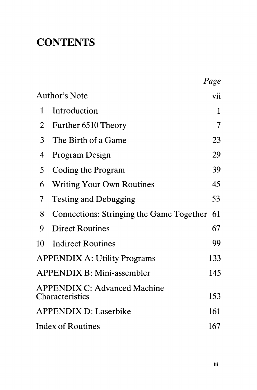
CONTENTS

Page

Author’s Note vii

1 Introduction 1

2 Further 6510 Theory 7
3 The Birth of a Game 23
4 Program Design 29
5 Coding the Program 39

6 Writing Your Own Routines 45

7 Testing and Debugging 53

8 Connections: Stringing the Game Together 61

9 Direct Routines 67

10 Indirect Routines 99

APPENDIX A: Utility Programs 133

APPENDIX B: Mini-assembler 145

APPENDIX C: Advanced Machine
Characteristics 153

APPENDIX D: Laserbike 161
Index of Routines 167

iii

Contents in detail

CHAPTER 1

Introduction
The process of writing games, how this book is set out, interrupts and
the 64, machine code and BASIC.

CHAPTER 2

Further 6510 Theory
The workings of the 6510 and 6502 chips, addressing techniques, the
stack, multi-bit operations, logical operations, scanning the screen,
multiplication and shifts, data structures and tables.

CHAPTER 3

The Birth of a Game
Beginning to write games in BASIC and/or machine code, the essential
ingredients of a good game, developing your game idea.

CHAPTER 4

Program Design
Drawing up charts to divide the game into a series of minor tasks,
looking at top-down charts, how charts help in writing programs.

CHAPTER 5

Coding the Program
Functional routines, parameter passing, compiling routines, parameter
clashes, assemblers.

CHAPTER 6

Writing Your Own Routines
How to write your own routines, turning algorithms into machine code

routines, the development of a Spiral Screen Fill routine, algorithm
design to stimulate your brain to solve problems and produce new
routines.

CHAPTER 7

Testing and Debugging
The causes of bugs, keeping routines simple, testing the routines,
debugging.

v

Machine code games routines for the Commodore 64

CHAPTER 8

Connections: Stringing the Game Together
What connections need to be made, iteration, DO-UNTIL loops,
conditional branching, checking bugs in connectors.

CHAPTER 9

Direct Routines

Text and slow printing, Filling memory, Copying memory, Delays,

Updating bombs, Scrolling, Interaction, Inverting and Explosions,

Alternative sprite system.

CHAPTER 10

Indirect Routines

The interrupt, Sprites, Further uses of UDGs, Sound, Large-scale

games, Fleet movements, Random numbers, Non-linear motion, Color

memory.

APPENDIX A

Utility Programs

Recovering a crashed program, siting the program and memory

management, entering machine code from BASIC, user-definable
graphics and a UDG editor, sprites and a sprite editor.

APPENDIX B

Mini-assembler

BASIC assembler including a disassembler, program description, using

the program, Mini-assembler listing, user-definable function keys,

dynamic halt, quotes-mode alleviator, sound and sprite mute,

Mini-toolkit.

APPENDIX C

Advanced Machine Characteristics

The keyboard and its buffer, BASIC text and variable storage, the

CIAs, SID and VIC memory maps.

APPENDIX D

Laserbike
Complete game listing.

VI

Author’s Note

Here is a collection of routines, methods and techniques which are all
useful in the construction of games. I have had great pleasure in

compiling this list — I have discovered much about the machine that I

didn’t know before. There were many routines that couldn’t be listed in
this book for various reasons. The ones listed here, however, should
suffice to give you a head-start in the world of machine code games
programming. Don’t stick rigidly to my methods and ideas: let yourself
develop as you feel you should. I am totally self-taught and thus have

my own particular style.

This book is designed to be more than just a collection of routines. All
the ideas are explained so that you can confidently alter them, mix them
and tease them apart. Don’t just type them in and use them — do them
justice.

Throughout the book I refer to both the 6502 and the 6510. This is a
matter of loyalty. As far as programming is concerned, the two are
identical. I had been programming the 6502 years before the 64 arrived,
so I feel a certain amount of afinity for it.

On a final note I would like to thank my friends and family who bore
with me and offered helpful suggestions while I wrote the book.

Program notes

In the computer listings in this book, the following symbols have been
replaced. Please ensure that you key in the correct sign.

£ appears as \

appears as —

| appears as A

Commands which appear in the listings in square brackets are listed
below:

[CLS] - Clear Screen [HOM] - Cursor Home
[CD] - Cursor Down

[CU]

- Cursor Up

[CL] - Cursor Left

[CR]

- Cursor Right

[RVS] - Reverse On

[OFF] - Reverse Off

[FX] - Function Key X (eg [FI]

, [F2])

Vll

CHAPTER 1

Introduction

The language of BASIC is remarkable in two ways: it’s remarkably
simple to learn and apply and it’s remarkably slow. Machine code is also
simple to learn (although much harder to write) but is remarkably fast.
When the two are mixed a hybrid form of programming evolves: one
that is simple to use yet fast. Ideally the best programs are written in 100
per cent machine code, but to write programs like this demands a lot of
practice and experience. A mixture provides the best of both worlds.
This book is about using machine code in games in this way. Writing
pure machine code is simply a logical extension of some of the ideas, but
don’t rush it, it’ll come naturally.

The problem with machine code is that it’s difficult to be objective.
The instructions themselves are so ridiculously elementary that any

large task seems daunting to say the least. By contrast, BASIC lends
itself well to the construction of longer, more complex programs.

Look at it in this way. By now you probably ‘think in BASIC’ quite

comfortably. When you start to learn French at school, the language
seems very abstract but, after a time, the ability to think in the language
itself becomes easier. The same is true of machine code. After a while

you will develop a feel for the language proper. Mixing machine code
with BASIC is a powerful way of learning. The more you do it, the
bigger the role machine code will take in your games and, on top of this,
you will minimise the amount of time needed to write a decent game.
The ‘balance of the game’ is an important idea and the keynote in

machine code programming is simplicity. Keep the amount of machine
code down to start with and work up gradually, while keeping the

machine code itself simple.

Writing games

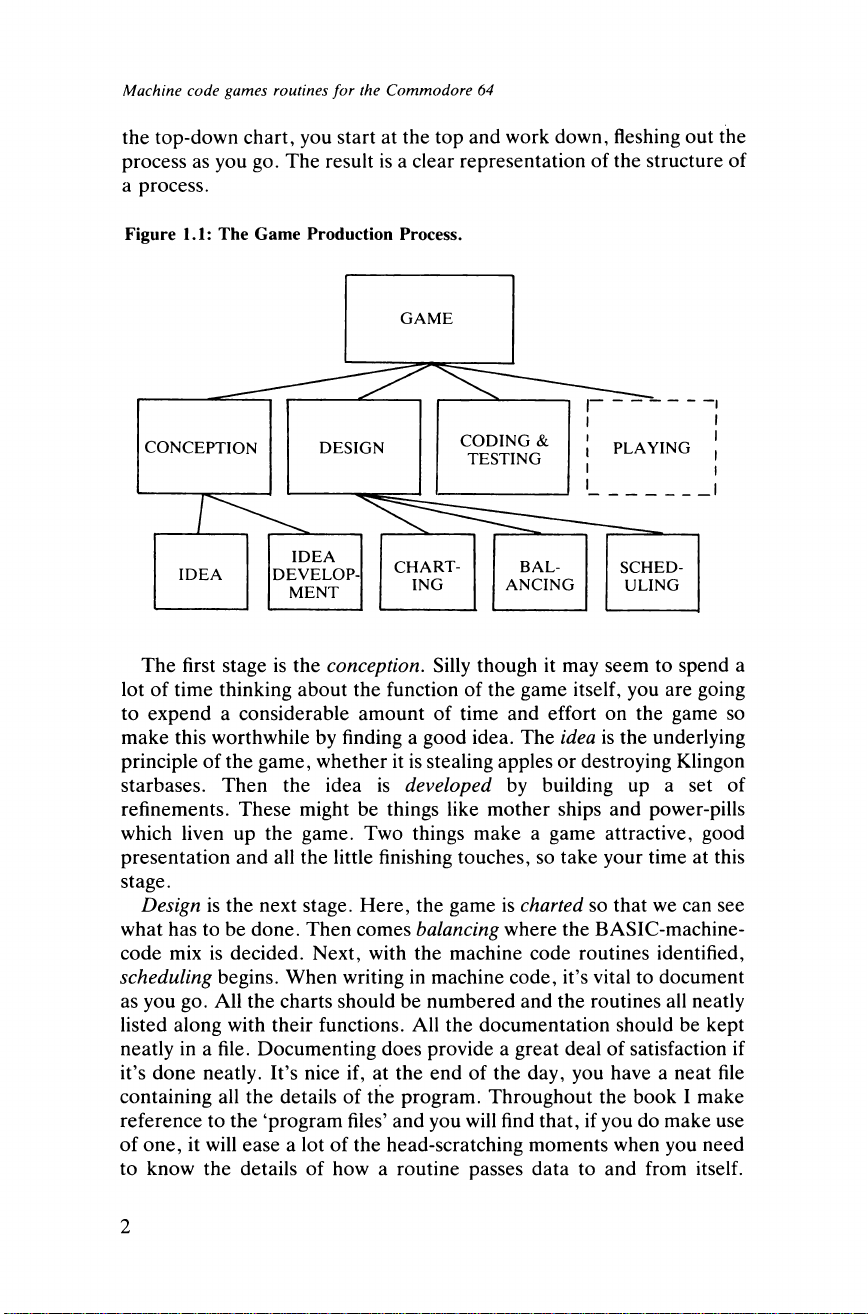
Figure 1.1 illustrates the process of writing a game. Each stage, right
from the first idea, is examined in detail. You start at the left and work
steadily to the right. By the time you get there, you have a working
game. This type of chart is known as a top-down chart (you’ll be seeing a

lot of charts so get used to them — although they are all very basic). In

1

Machine code games routines for the Commodore 64

the top-down chart, you start at the top and work down, fleshing out the
process as you go. The result is a clear representation of the structure of
a process.

Figure 1.1: The Game Production Process.

The first stage is the conception. Silly though it may seem to spend a
lot of time thinking about the function of the game itself, you are going
to expend a considerable amount of time and effort on the game so
make this worthwhile by finding a good idea. The idea is the underlying
principle of the game, whether it is stealing apples or destroying Klingon
starbases. Then the idea is developed by building up a set of
refinements. These might be things like mother ships and power-pills
which liven up the game. Two things make a game attractive, good
presentation and all the little finishing touches, so take your time at this
stage.

Design is the next stage. Here, the game is charted so that we can see
what has to be done. Then comes balancing where the BASIC-machine-
code mix is decided. Next, with the machine code routines identified,

scheduling begins. When writing in machine code, it’s vital to document

as you go. All the charts should be numbered and the routines all neatly
listed along with their functions. All the documentation should be kept
neatly in a file. Documenting does provide a great deal of satisfaction if
it’s done neatly. It’s nice if, at the end of the day, you have a neat file

containing all the details of the program. Throughout the book I make
reference to the ‘program files’ and you will find that, if you do make use
of one, it will ease a lot of the head-scratching moments when you need
to know the details of how a routine passes data to and from itself.

2

Chapter 1 Introduction

Returning to scheduling, this simply means looking at the program files
and planning a programme (not program) of coding, testing and
documenting so that you can work to set deadlines.

Coding and testing is where the game really gets under way. This is
the process of constructing routines to perform various operations and
fiddling around until they work. After all this is done, the program is
finished and playing can commence.

The routines

As the title says, this book contains a wealth of machine code routines.

These perform a lot of simple and complex tasks that help take the

pressure off BASIC programs. However they are not intended for you

just to copy in and forget about. If you are going to use a routine, then
take the trouble to see how it works — you may have to make

alterations to it and, if you don't understand it, then modifying becomes
impossible. As this was the intention, the routines are accompanied by a
description of the topic, how the machine code program works and
occasionally a few points on style in the programs. The routines
themselves are annotated with short remarks and program flow is shown
by arrows so that, at a glance, you can make cross references to the
flowcharts that go with them. The result of all this support is that they
are more than just routines, they are methods and techniques. The

routine section itself is divided into two — direct and indirect. The
direct routines perform fairly clearcut tasks such as filling memory or
scrolling while the indirect section concerns itself with concepts

(supported by routines) such as moving fleets of objects around the
screen.

The book

Not all the routines in the book are contained in that section though.
You will find them hidden all over (they are listed in the routine index at
the end of the book) often just to prove a point to make it interesting.
The appendices also contain more important information such as using
the function keys as well as a collection of utility programs. The idea is
that this book can be read and not used merely as a dry reference guide.
I would suggest that you read the book before starting on a program as
you may miss out on an idea which you could be using in a program.

Don’t rush reading it through. I spend a lot of time ‘dabbling around’
with ideas, which is the only way to really get to know the machine and
these routines. Play with them, alter them and tease them apart until
you're really familiar with them. I find it all too easy to spend an hour
happily toying around with ideas. If you’re not really familiar with

3

Machine code games routines for the Commodore 64

machine code, then you won’t understand its quirks; these will confront
you and you won’t know what’s happening. It can be very depressing —
a computer is a very strict teacher, and allows no mistakes.

Talking about mistakes, no machine code program is ever without
them. This normally culminates in a hang-up. When this happens don’t
panic — just worry about your program. Often the RUN/STOP +
RESTORE sequence will release you. Don’t forget to make backup
copies every half-hour or so and don’t write a backup over the top of a

previous backup — you will corrupt the old backup and acquire a write

error with the new one. Don’t forget to verify all your backups. It does
take time with a tape system but it’s worth it if you have a powercut. If

the machine is still jammed, then a little routine in Appendix A (Crash

Recovery) will pluck you out — have a look now.

At first, to make sure that the routines you need are in the book, you
might try writing a game around a routine or two instead of writing the
routines around a game. For instance, you might take the sprite homing
routine (Chapter 10 — this homes sprites 1 to 7 on to the position of
sprite 0) and write a chase game where the player controls sprite 0 with a

joystick (also in Chapter 10) and has to perform certain tasks on the

screen without colliding with a homing sprite. A program like this is
easily written and will run quickly (especially if the routines are hooked
on to the interrupt).

Interrupts

Interrupts are a major tool in the harnessing of the 64. You may not
understand the term interrupt now, but by the end of the book you will.

The interrupt is definitely the key to the machine. In the two routine
chapters, many of the routines are specially designed to run on the

interrupt, including a tune-player: when something is ‘on the interrupt’ it
means that the 64 is automatically calling the routine for you. Thus you

can have all eight sprites tearing around the screen while listing and
editing the program with a flashing cursor (this will amaze your friends).
All I can say is that, if you don’t like using interrupts, then you won’t
capitalise on the 64. Some of the routines in Appendix B show you how
to use the function keys properly to do some remarkable things.

Machine code

To finish off this introductory section, I’ll just point out a few important
facts. First, writing in machine code takes more time than BASIC.
Programming starts off with great enthusiasm. However, after this there
is a considerable period when you’re not going to get results — the
slump. Many would-be programmers give up at this stage, which results

4

Chapter 1 Introduction

in unfinished programs. Machine code programming is all about
stamina, determination and confidence. Start off with simple routines
and work up to the big ones.

Another important point is that there are an almost infinite number of
ways of writing a program to perform a task. My routines are simply one
way of doing this. Often you will be able to shorten them as they are
designed to show you how they work and not to show off the ‘clever
tricks’ that abound in machine code. The same idea goes for the process
of games programming. Mine is simply a guideline and everybody
develops their own particular style. Wait until you are confident and
then develop your own style.

When writing your own routines keep them simple. If you look at
the arrows on my routines, you will see they are few and are nested one
inside the other. When branching is thrown in anywhere the bugs creep
in. Keep it simple. Often badly-written routines arise because the

programmer writes them at the keyboard. For the really simple ones this
is alright but I have noticed that the screen itself doesn’t help
concentration. Most of my routines are sketched out on paper first and
then transferred. As I have got into this habit I write my routines
anywhere (anyway staring at a TV screen for too long is bad for you).

The question of assemblers must arise at this stage. While hand
assembly is good for teaching the fundamentals, an assembler is vital for
those longer routines. The best tactic is to get hold of a plug-in cartridge
assembler. Personally I have several assemblers including a retired
Acorn Atom which I sometimes use in parallel with my 64. If you must
hand assemble then be wary of branch vectors (which can be tricky to
calculate by hand). There is an assembler in Appendix B, at the back of

the book, which doubles as a disassembler. Whether or not you have an

assembler, the adressing mode representation in this book (shown in

Table 2.2 in the next chapter) is probably not the one you are used to.
The reason for the difference is an effort on my part to force you to
comprehend the routines without blindly typing them in.

I say some pretty harsh words about BASIC in this book but this is

not designed to stop you from using it. It remains the greatest computer
language yet devised. Programs can be quickly and efficiently put
together. Throughout the book I use BASIC to demonstrate some
principles. Don’t drop BASIC — it’s great. If you’re ready then start
reading through the book. You’ll find all sorts of useful information, so
read on!

5

CHAPTER 2

Further 6510 Theory

Some of the methods used in this book may seem a little strange at first,
and this chapter is designed to explain the theory behind these ideas. If
you know about the workings of the 6510 and 6502 anyway, skip this
chapter. Quite a few topics will be covered and it’s imperative for
effective programming that you are totally au fait with them. The best
advice is to play around with these ideas until you can use and think of
them instinctively. Mastery of anything is when you can do something
without really having to think at all.

The ideas presented here are simply the ones I use. Don’t just use

them, try working with 32-bit or 64-bit numbers as opposed to 8 and 16
bits. If you stretch your abilities then success is guaranteed.

Addressing techniques

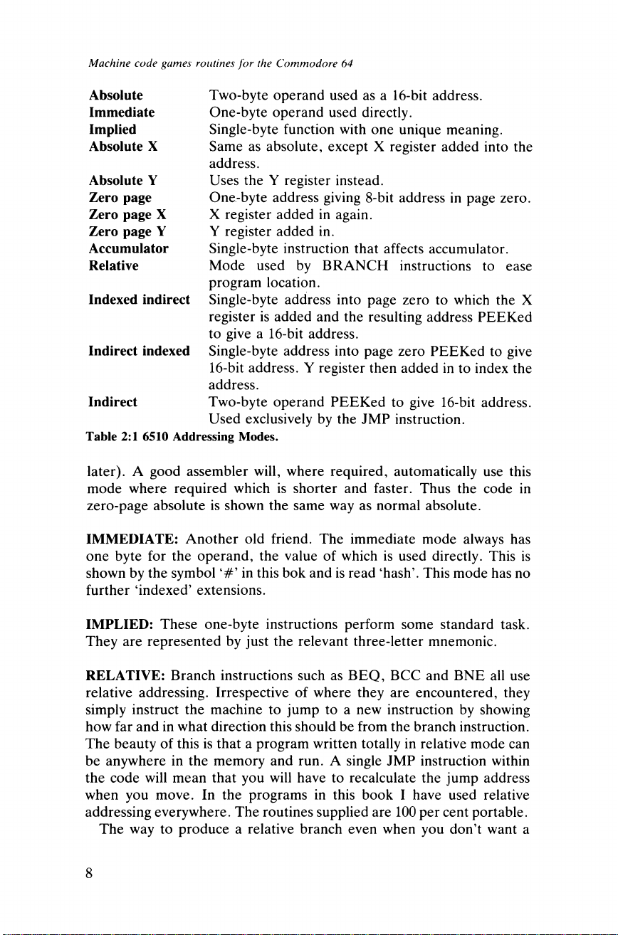
The 6510 processor has no less than 13 different addressing modes! Stop

now and see how many you can remember. For every forgotten mode
there is lost opportunity. Not only should you know them all but you
should be able to decide instantly which is the best for the problem in
hand. Table 2.1 gives all the modes. How many do you know
thoroughly?

The chances are you did pretty badly in that test. Returning to our
earlier analogy, addressing modes are like tenses in French: you can get
by on one or two but only just. Read on and discover the uses of the
more obscure modes.

ABSOLUTE: Absolute mode is very important. It takes a 16-bit
operand and uses that as the address. Many of the other modes are
based on this one. In this book the absolute mode is denoted by just the
operand, eg:

LDA 1024

which PEEKs the first byte of the screen. A close relative is the
zero-page absolute mode which is identical except that it has only a
one-byte operand which is a page-zero address (more about page-zero

7

Machine code games routines for the Commodore 64

Absolute
Immediate
Implied
Absolute X

Absolute Y
Zero page
Zero page X
Zero page Y
Accumulator
Relative

Indexed indirect

Indirect indexed

Indirect

Two-byte operand used as a 16-bit address.
One-byte operand used directly.
Single-byte function with one unique meaning.
Same as absolute, except X register added into the
address.
Uses the Y register instead.
One-byte address giving 8-bit address in page zero.
X register added in again.
Y register added in.
Single-byte instruction that affects accumulator.
Mode used by BRANCH instructions to ease
program location.
Single-byte address into page zero to which the X
register is added and the resulting address PEEKed
to give a 16-bit address.
Single-byte address into page zero PEEKed to give
16-bit address. Y register then added in to index the
address.
Two-byte operand PEEKed to give 16-bit address.
Used exclusively by the JMP instruction.

Table 2:1 6510 Addressing Modes.

later). A good assembler will, where required, automatically use this
mode where required which is shorter and faster. Thus the code in
zero-page absolute is shown the same way as normal absolute.

IMMEDIATE: Another old friend. The immediate mode always has
one byte for the operand, the value of which is used directly. This is
shown by the symbol‘# ’ in this bok and is read ‘hash’. This mode has no
further ‘indexed’ extensions.

IMPLIED: These one-byte instructions perform some standard task.
They are represented by just the relevant three-letter mnemonic.

RELATIVE: Branch instructions such as BEQ, BCC and BNE all use
relative addressing. Irrespective of where they are encountered, they
simply instruct the machine to jump to a new instruction by showing

how far and in what direction this should be from the branch instruction.
The beauty of this is that a program written totally in relative mode can
be anywhere in the memory and run. A single JMP instruction within
the code will mean that you will have to recalculate the jump address
when you move. In the programs in this book I have used relative
addressing everywhere. The routines supplied are 100 per cent portable.

The way to produce a relative branch even when you don’t want a

8

Chapter 2 Further 6510 Theory

condition to be true is to precede the branch instruction by the
appropriate implied instruction:

CLC
BCC

or

SEC
BCS

Both of these will ‘force’ the branch. When you see this happening in
the code, you’ll understand what’s going on. If you want to branch to a
location that’s out of range of the branch then you’re probably doing
some bad programming. If you can’t avoid it then reverse the branch
instruction (ie BCC becomes BCS and BPL becomes BMI) and place a
JMP after it.

Look at this example:

BEQ LOOP
RTS

Suppose this gives an out-of-range error. The answer is the following
code:

✓ BNE STOP

(JMP LOOP

:STOP ARTS

This is an ‘extended’ branch and should be used in preference to a

leap-frogging technique, although locatability is lost.

At this stage it might be wise to discuss the ways in which variables
and labels are presented in the book. Labels are preceded by a ‘:’ sign
and are written in a column well to the left of the code. Variables are
simply short meaningful groups of letters that represent some value (eg
LDA CHAR has CHAR as a variable). You could interpret this in two
ways: either CHAR is the address of the value of CHAR and the
instruction is thus absolute, or CHAR is the value itself making the
instruction immediate. The choice is completely yours. For various
reasons, I have used LLX for labels throughout the code as labels where
X is any number. The routine is usually started by :LL0, and :ILL1

:ILL2, etc, appear in the order I used them when compiling the routine.
As each routine uses the same labels you are forced to develop your own
labels — an aid to success.

ZERO-PAGE THEORY: In this summary of addressing techniques, a

9

Machine code games routines for the Commodore 64

quick word on page-zero will not be out of place. Page-zero is the core

of the computer’s memory. It is the area which has modes devoted to it,

and so these modes tend to be fast and effective. You will see that the 64

doesn’t leave a lot of space for the programmer here but there’s enough.

The beauty of page-zero is that you only need a one-byte operand to

address the 256 bytes in the page. The result is more space (this

shouldn’t be a consideration) more speed and versatility. If you look in

the manual you’ll find page-zero is full of all sorts of interesting things.

Thus where possible use addresses in the range 2-255. Locations 0 and 1

contain ports arid should be kept clear of.

ABSOLUTE X and Y: These are close relations of the absolute mode. A

16-bit address is given and to this is added the value of either the X or Y
registers. This means that one instruction can produce 256 different
addresses. This mode is used to produce very short fill and scroll
routines amongst other things. The mode is represented by adding the
suffix \X ’ or ‘,Y’ to the operand.

The instruction LDA 1024,X could PEEK any number from 1024 to

1279 merely by altering the X register. There is also a zero-page
counterpart for this but only with the X register. (There is a Y register
mode, but it’s very limited.)

INDIRECT: This mode is used purely with the JMP instruction and is
not used in the book, but it is very handy for picking up a vector. A

16-bit operand is used and this points to a pair of memory locations.

These are then PEEKed and the address so obtained is jumped to. JMP

(788) means look at 788 and 789, use their contents as a 16-bit address

and jump to that address. The mode is signified here by enclosing the
address in a pair of brackets.

ZERO-PAGE INDEXED MODES: These modes are useful, as the
operative address can be changed to cover the entire memory of the 64.
What happens is that the instruction points to a zero-page address. The
value found at this address constitutes a 16-bit number which then
becomes the operative address. On top of this, more flexibility is given
by adding the values of the X and Y registers. There are two variations,
where the value is added in before and where it is added in afterwards.
One uses the X register and the other uses the Y.

INDEXED INDIRECT: This is the X register associated mode. The
operand is a zero-page address to which the value of the X register is
added (indexing). The resulting zero-page address is then PEEKed and

the result of the PEEK supplies a 16-bit address (indirect). Look at

Figure 2.1 to see this in action.

10

Chapter 2 Further 6510 Theory

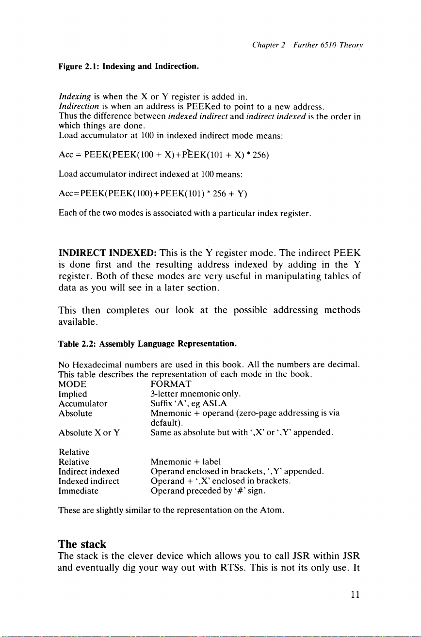
Figure 2.1: Indexing and Indirection.

Indexing is when the X or Y register is added in.
Indirection is when an address is PEEKed to point to a new address.

Thus the difference between indexed indirect and indirect indexed is the order in
which things are done.
Load accumulator at 100 in indexed indirect mode means:

Acc = PEEK(PEEK( 100 + X) + PEEK(101 + X) * 256)
Load accumulator indirect indexed at 100 means:
Acc=PEEK(PEEK(100) + PEEK(101) * 256 + Y)
Each of the two modes is associated with a particular index register.

INDIRECT INDEXED: This is the Y register mode. The indirect PEEK
is done first and the resulting address indexed by adding in the Y
register. Both of these modes are very useful in manipulating tables of
data as you will see in a later section.

This then completes our look at the possible addressing methods

available.

Table 2.2: Assembly Language Representation.

No Hexadecimal numbers are used in this book. All the numbers are decimal.
This table describes the representation of each mode in the book.

MODE

FORMAT
Implied
Accumulator
Absolute

Absolute X or Y

3-letter mnemonic only.

Suffix \A\ eg ASLA

Mnemonic + operand (zero-page addressing is via

default).

Same as absolute but with \X’ or \Y ’ appended.
Relative

Relative
Indirect indexed
Indexed indirect
Immediate

Mnemonic + label

Operand enclosed in brackets, \Y ’ appended.

Operand -I- \X ’ enclosed in brackets.

Operand preceded by ‘# ’ sign.

These are slightly similar to the representation on the Atom.

The stack

The stack is the clever device which allows you to call JSR within JSR
and eventually dig your way out with RTSs. This is not its only use. It

11

Machine code games routines for the Commodore 64

can also be used to pass parameters and store variables, but first let’s see

how it works.

The stack occupies page 1 of the 64’s memory. A stack pointer
maintains the position within the stack. Every time a JSR is
encountered, the return address is stored on the stack, the stack pointer
adds 2 and a JMP (effectively) is called to the subroutine address. On
finding an RTS the stack pointer is lowered, an address is pulled off and
a JMP is executed to this address. As the stack is 256 bytes long, it’s
possible to nest 128 consecutive JSR calls before overwriting the first
return address: don’t try to do this because all sorts of other things use

the stack as well, and if it fills up you’ll know all about it!

The instructions PHA and PLA mean PusH and PulL the
Accumulator to and from the stack. Obviously if you do push something
on, you’ll have to wait until the stack pointer is in the right position to

remove it. Manipulation of the stack pointer itself can be done with the
aid of TSX (Transfer Stack pointer to X) and TXS which puts it back. If
you are doing this, be careful not to alter any return address.

Using these ideas, we might store the value in the X register within a
routine with no JSR, RTS or other stack operations between by using a
TXA, PHA. Recovery is the opposite — PLA , TAX. Admittedly this is
not very helpful but if we want to pass a parameter it can be a helpful
way to send it. In the absence of a zero-page location, the stack provides

a handy temporary storage facility. The processor status register can
also be stored and removed from the stack by PHP and PLP. When an
interrupt occurs, the stack is used to store all register values and the
status register so that on return nothing seems to have happened.

Multi-bit operations

It’s easy to add two 8-bit numbers. But as soon as we use more than

eight bits, things begin to get a little more complicated. You probably

know how to add 16-bit numbers: this section is to remind you and show

you why things are done. The first thing we shall look at is addition. If
you understand it now then write a 64-bit adding routine — this will test
your knowledge.

The first thing to do is to clear the carry flag. This is because ADC
means ‘ADd with Carry’. A number is added into the accumulator and,
if the carry flag is set, an extra 1 is added in as well (a smart way to add
two numbers and increment the result is to use a SEC). Now if the last
operation overflowed the accumulator, the carry flag is set to 1. When
the next (more significant) bytes are added the carry is not cleared. If an
overflow occurred, then an extra 1 must be added. The process is like
adding decimal numbers: when a column exceeds nine you must carry a
ten over into the next column where it appears as a one. Only the first

12

Chapter 2 Further 6510 Theory

CLC is needed for the entire operation. The following code adds two

16-bit numbers found in 251-252 and 253-254:

LDA 251
CLC
ADC 253
STA 253
LDA 252
ADC 254
STA 254

Subtraction is performed in the same manner except that SEC is used to
SEt the Carry beforehand. Addition and subtraction are vital in games

as they allow us to move objects around the screen.

A vector is a number. In the manual you will see vectors which point
to the start of ROM routines. In games terms, a vector is a number that
is added into an address to simulate movement. When I speak of adding
in a vector, I mean adding in a number to update a position. For
example to move a sprite to the right you add in the vector 1 to its X
coordinate. By definition, a vector has both magnitude and direction.
Both of these can be contained within a number: a faster right
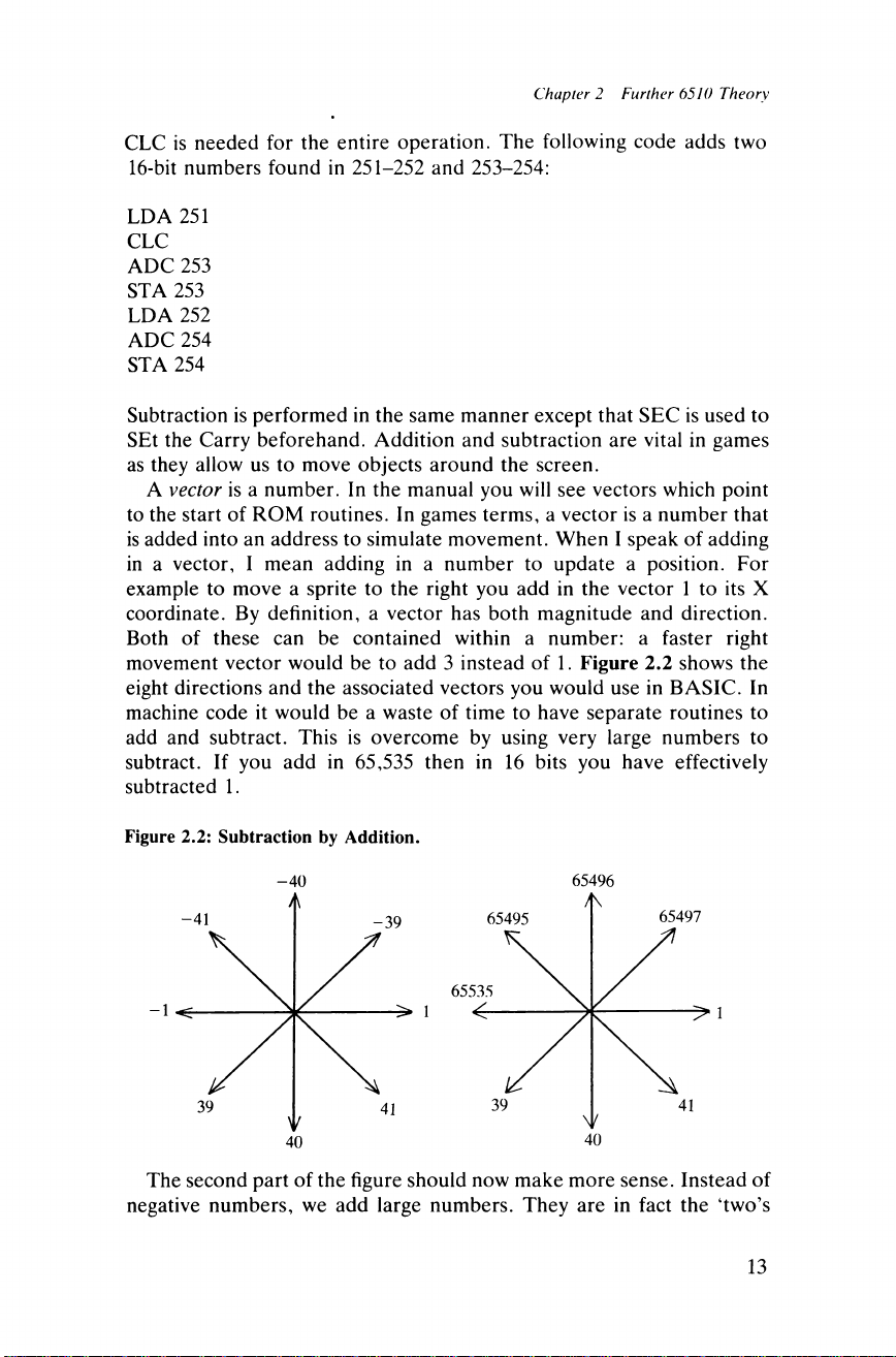
movement vector would be to add 3 instead of 1. Figure 2.2 shows the
eight directions and the associated vectors you would use in BASIC. In
machine code it would be a waste of time to have separate routines to
add and subtract. This is overcome by using very large numbers to

subtract. If you add in 65,535 then in 16 bits you have effectively
subtracted 1.

Figure 2.2: Subtraction by Addition.

-40 65496

The second part of the figure should now make more sense. Instead of

negative numbers, we add large numbers. They are in fact the ‘two’s

13

Machine code games routines for the C ommodore 64

complement' of the negative numbers. This idea of using large numbers
to perform subtraction is extensively used and so you should ensure that
you fully understand it.

Comparing two numbers for similarity or difference is simple. You
just use CMP (or CPX or CPY) and use BEQ (similar) or BNE

(different). Working in 16-bits, a little more must be done. Often you
must check to see if an address has been reached (or a missile has hit a
ship) in which case a 16-bit comparison is needed. The process is simple:
compare the two lower bits and the two higher bits separately. If the two
lower bits don't match then the numbers must be different. If they do
match then test the higher two bytes. Either they match (both numbers

are the same) or they don’t. The routine does this:

LDA 251

CMP 253

BNE UNEQUAL

LDA 252

CMP 254

BNE UNEQUAL

**Numbers are equal**

The two numbers are stored in 251-252 and 253-254. UNEQUAL is

simply a label for the sake of demonstration.

These 16-bit operations are very important. They form the core of
writing a game in machine code; without them you cannot move objects
around with any degree of ease.

Logical operations

The AND/OR/EOR functions always seem a little strange as they have

no apparent use. In fact they make the manipulation of individual bits

within a byte very easy indeed. Often you will want to set just a bit in a
byte or clear a few bits somewhere else without disturbing the rest. The
key to this is the use of the logical operators. Each does its own little
thing and Figure 2.3 will refresh your memory as to their function.

AND: The result of AND is 1 only, and only if both the first input AND
the second input are 1. Thus 1101 AND 1100 = 1100. The AND
function is a mask operation. It enables you to mask out unwanted bits
while retaining the important parts. Suppose we were interested in the
lower three bits of an 8-bit number. To obtain these bits only, we mask
with 1 + 2 + 4 = 7. Only where a 1 is present in the mask can a 1 show
through. By this method we can do all sorts of things: checking whether
a number is even or odd, or decoding a byte that contains more than one

14

Chapter 2 Further 6510 Theory

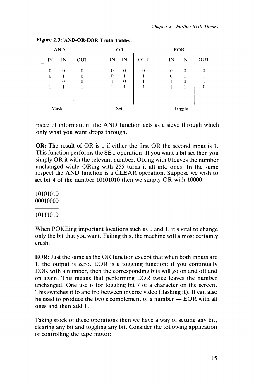
Figure 2.3: AND-OR-EOR Truth Tables.

AND

IN IN OUT

0

0

0

0 1 0

1
101

0

1

Mask

OR

IN

IN

OUT

0 0 0
0 1 1

110

1

1
1

Set

EOR

IN IN

OUT

0

0

0

0

1
1

1

0

1

1
1

0

Toggle

piece of information, the AND function acts as a sieve through which
only what you want drops through.

OR: The result of OR is 1 if either the first OR the second input is 1.
This function performs the SET operation. If you want a bit set then you
simply OR it with the relevant number. ORing with 0 leaves the number
unchanged while ORing with 255 turns it all into ones. In the same

respect the AND function is a CLEAR operation. Suppose we wish to

set bit 4 of the number 10101010 then we simply OR with 10000:

10101010

00010000

10111010

When POKEing important locations such as 0 and 1, it’s vital to change
only the bit that you want. Failing this, the machine will almost certainly
crash.

EOR: Just the same as the OR function except that when both inputs are

1, the output is zero. EOR is a toggling function: if you continually

EOR with a number, then the corresponding bits will go on and off and
on again. This means that performing EOR twice leaves the number
unchanged. One use is for toggling bit 7 of a character on the screen.

This switches it to and fro between inverse video (flashing it). It can also

be used to produce the two’s complement of a number — EOR with all

ones and then add 1.

Taking stock of these operations then we have a way of setting any bit,
clearing any bit and toggling any bit. Consider the following application
of controlling the tape motor:

15

Machine code games routines for the Commodore 64

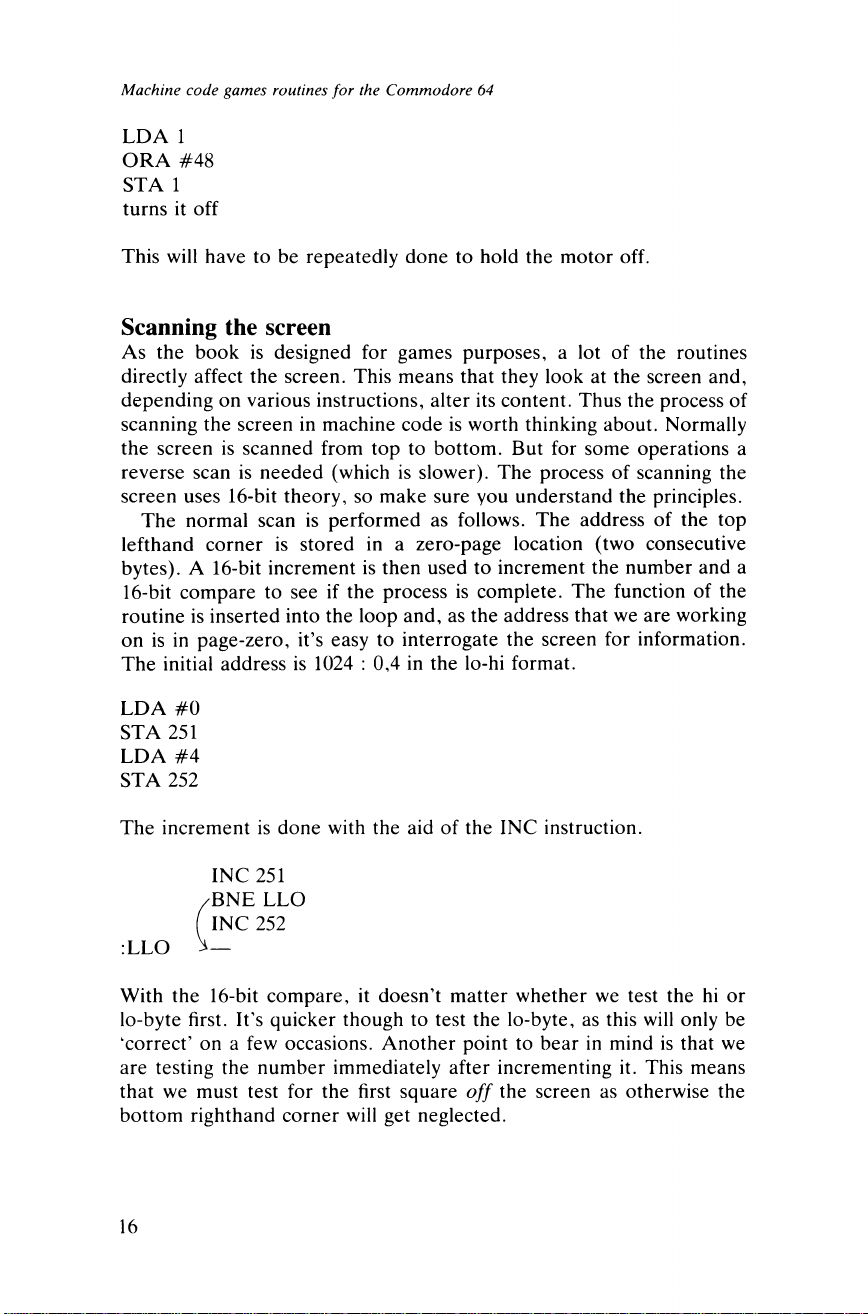
LDA 1
ORA #48
STA 1
turns it off

This will have to be repeatedly done to hold the motor off.

Scanning the screen

As the book is designed for games purposes, a lot of the routines

directly affect the screen. This means that they look at the screen and,

depending on various instructions, alter its content. Thus the process of

scanning the screen in machine code is worth thinking about. Normally

the screen is scanned from top to bottom. But for some operations a

reverse scan is needed (which is slower). The process of scanning the

screen uses 16-bit theory, so make sure you understand the principles.

The normal scan is performed as follows. The address of the top
lefthand corner is stored in a zero-page location (two consecutive
bytes). A 16-bit increment is then used to increment the number and a

16-bit compare to see if the process is complete. The function of the

routine is inserted into the loop and, as the address that we are working
on is in page-zero, it’s easy to interrogate the screen for information.
The initial address is 1024 : 0,4 in the lo-hi format.

LDA #0
STA 251
LDA #4
STA 252

The increment is done with the aid of the INC instruction.

INC 251

/BNE LLO

( INC 252

:LLO

With the 16-bit compare, it doesn’t matter whether we test the hi or

lo-byte first. It’s quicker though to test the lo-byte, as this will only be
'correct’ on a few occasions. Another point to bear in mind is that we

are testing the number immediately after incrementing it. This means
that we must test for the first square off the screen as otherwise the
bottom righthand corner will get neglected.

16

Chapter 2 Further 6510 Theory

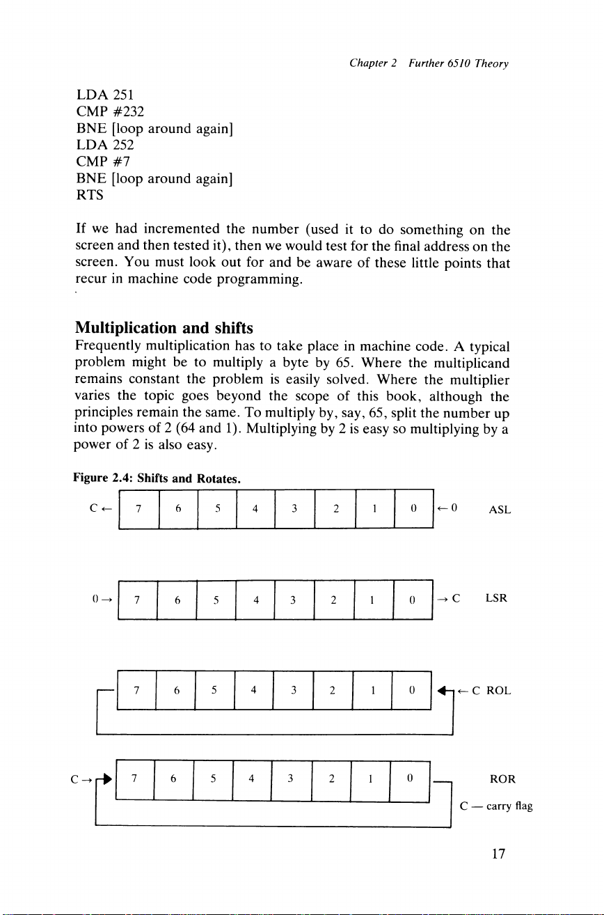
LDA 251
CMP #232
BNE [loop around again]
LDA 252
CMP #7
BNE [loop around again]
RTS

If we had incremented the number (used it to do something on the
screen and then tested it), then we would test for the final address on the
screen. You must look out for and be aware of these little points that
recur in machine code programming.

Multiplication and shifts

Frequently multiplication has to take place in machine code. A typical
problem might be to multiply a byte by 65. Where the multiplicand
remains constant the problem is easily solved. Where the multiplier
varies the topic goes beyond the scope of this book, although the
principles remain the same. To multiply by, say, 65, split the number up

into powers of 2 (64 and 1). Multiplying by 2 is easy so multiplying by a
power of 2 is also easy.

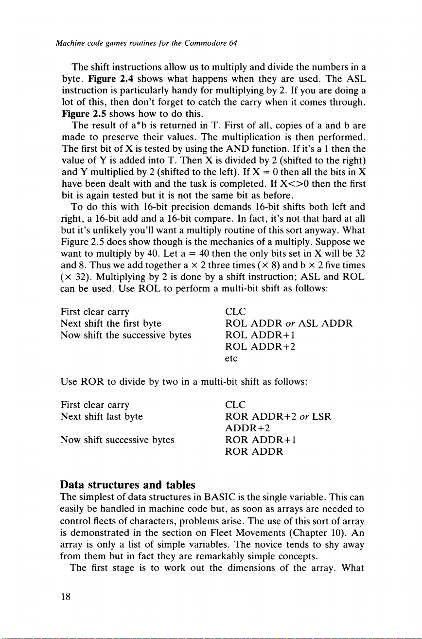
Figure 2.4: Shifts and Rotates.

17

Machine code games routines for the Commodore 64

The shift instructions allow us to multiply and divide the numbers in a

byte. Figure 2.4 shows what happens when they are used. The ASL
instruction is particularly handy for multiplying by 2. If you are doing a
lot of this, then don’t forget to catch the carry when it comes through.
Figure 2.5 shows how to do this.

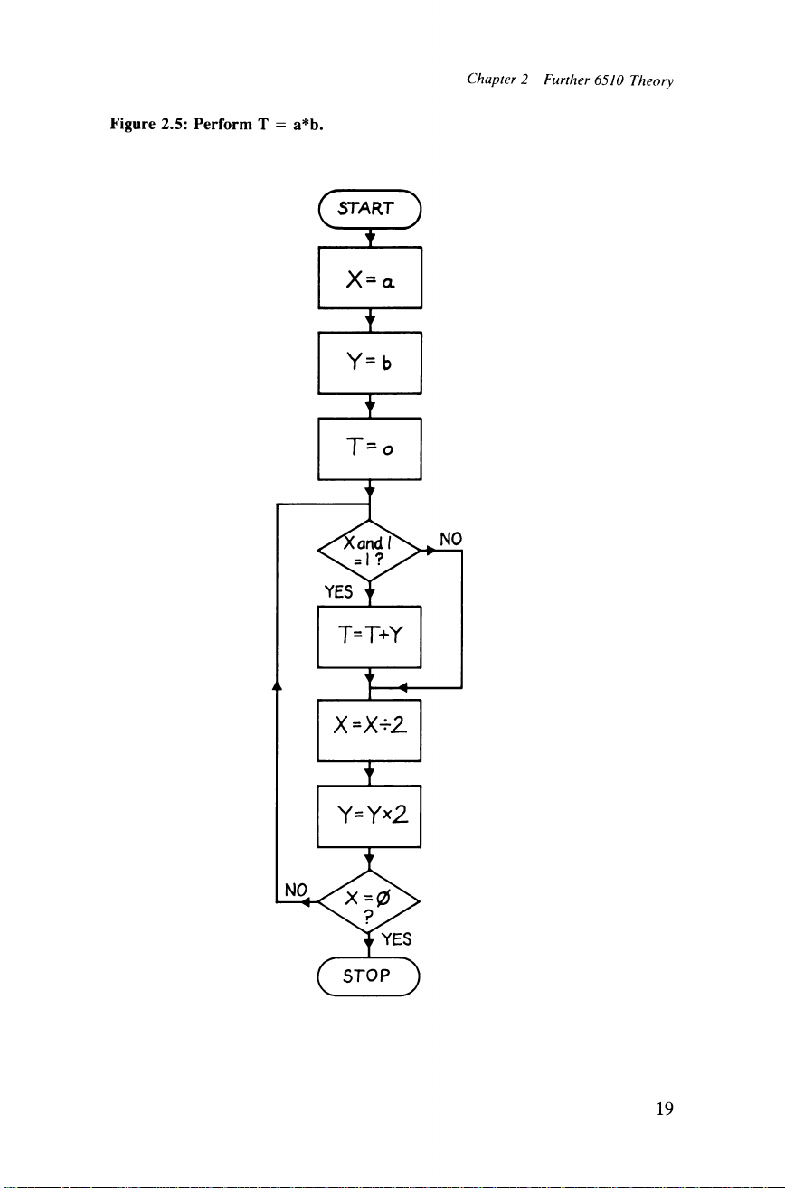
The result of a*b is returned in T. First of all, copies of a and b are

made to preserve their values. The multiplication is then performed.
The first bit of X is tested by using the AND function. If it’s a 1 then the
value of Y is added into T. Then X is divided by 2 (shifted to the right)

and Y multiplied by 2 (shifted to the left). If X = 0 then all the bits in X
have been dealt with and the task is completed. If X <>0 then the first
bit is again tested but it is not the same bit as before.

To do this with 16-bit precision demands 16-bit shifts both left and

right, a 16-bit add and a 16-bit compare. In fact, it’s not that hard at all

but it’s unlikely you’ll want a multiply routine of this sort anyway. What
Figure 2.5 does show though is the mechanics of a multiply. Suppose we
want to multiply by 40. Let a = 40 then the only bits set in X will be 32
and 8. Thus we add together a x 2 three times (x8) and b x 2 five times
(x 32). Multiplying by 2 is done by a shift instruction; ASL and ROL
can be used. Use ROL to perform a multi-bit shift as follows:

First clear carry CLC
Next shift the first byte ROL ADDR or ASL ADDR
Now shift the successive bytes

ROL ADDR+1
ROL ADDR+2
etc

Use ROR to divide by two in a multi-bit shift as follows:

First clear carry

CLC

Next shift last byte

ROR ADDR+2 or LSR
ADDR+2

Now shift successive bytes

ROR ADDR+1
ROR ADDR

Data structures and tables

The simplest of data structures in BASIC is the single variable. This can
easily be handled in machine code but, as soon as arrays are needed to

control fleets of characters, problems arise. The use of this sort of array
is demonstrated in the section on Fleet Movements (Chapter 10). An
array is only a list of simple variables. The novice tends to shy away
from them but in fact they are remarkably simple concepts.

The first stage is to work out the dimensions of the array. What

18

Chapter 2 Further 6510 Theory

Figure 2.5: Perform T = a*b.

( NO

19

Machine code games routines for the Commodore 64

information do you want held for each object? Some information, such
as an address, will need two bytes whereas others will need only one.
Let's suppose we want a table of 50 aliens containing an address, a
movement vector and an alien type. This might be represented by the
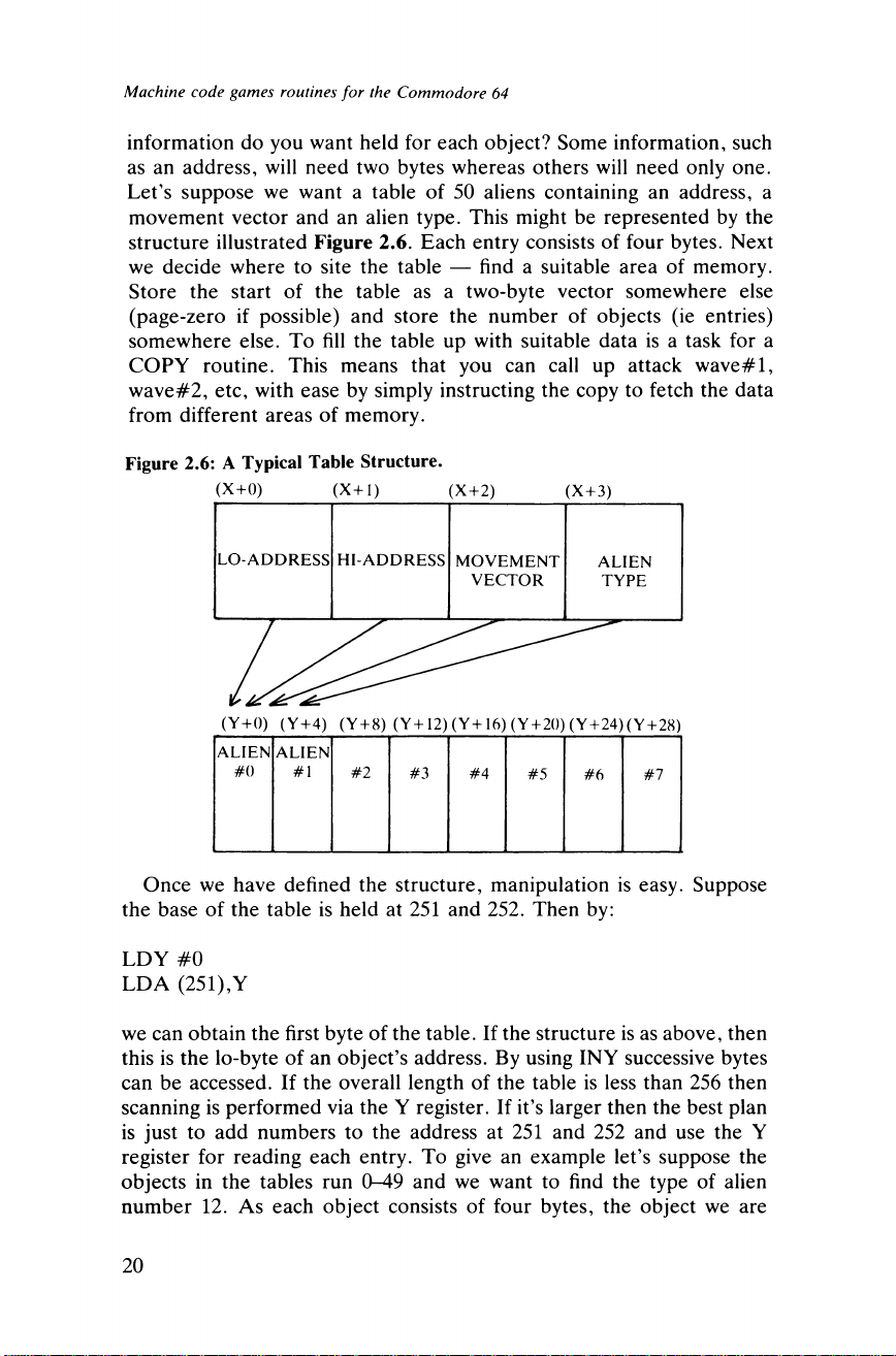
structure illustrated Figure 2.6. Each entry consists of four bytes. Next
we decide where to site the table — find a suitable area of memory.
Store the start of the table as a two-byte vector somewhere else
(page-zero if possible) and store the number of objects (ie entries)
somewhere else. To fill the table up with suitable data is a task for a
COPY routine. This means that you can call up attack wave#l,
wave#2, etc, with ease by simply instructing the copy to fetch the data
from different areas of memory.

Figure 2.6: A Typical Table Structure.

(X+0) (X +l ) (X + 2) (X + 3)

(Y + 0) (Y+4) (Y + 8) (Y +12 )(Y +1 6)( Y + 20)(Y + 24)(Y + 28)

ALIEN ALIEN

#0

#1

#2

#3

#4

#5

#6

#7

Once we have defined the structure, manipulation is easy. Suppose

the base of the table is held at 251 and 252. Then by:

LDY #0
LDA (251),Y

we can obtain the first byte of the table. If the structure is as above, then
this is the lo-byte of an object’s address. By using INY successive bytes
can be accessed. If the overall length of the table is less than 256 then
scanning is performed via the Y register. If it’s larger then the best plan
is just to add numbers to the address at 251 and 252 and use the Y

register for reading each entry. To give an example let’s suppose the
objects in the tables run 0-49 and we want to find the type of alien
number 12. As each object consists of four bytes, the object we are

20

Chapter 1 Introduction

interested in starts at Table + 12 * 4. Suppose 12 is in the accumulator.

Two ASLAs multiply by 4 and TAY moves the value into Y. The alien

type is the fourth (and final) byte of the object. Thus we follow with

three INYs. A LDA(251),Y then supplies the type of object #12.

Get type of object in accumulator

ASLA

ASLA

INY

INY

INY

LDA (251),Y

RTS

As you can see, tables are very easy to use. You will find them in use in

several of the routines in this book, including the screen-flash attribute

routine (Inverting and Explosions, Chapter 9) where a table of 25

elements is used to determine whether or not to flash that line.

21

CHAPTER 3

The Birth of a Game

So you have decided to write a machine code game. No doubt you

already have a rough idea of the game that you want, whether it is just
another variation on the Space Invader theme or a totally new idea of
your own. Whatever the case, don’t rush through this first stage. Before
you even think about moving on to the next part, put your thoughts
down on paper in a neat and ordered fashion. There is no way that you
are going to design a game (in machine code) if the basic idea varies
from day to day following your whims. In short, make up your mind
while you can. Once programming is under way, alterations will be
costly both in terms of time and morale.

Speaking of morale, this is one of the most important factors when
programming in machine code. There will be long periods of intense
work with little reward. It is a real test of stamina and self-confidence.
For this reason, it would be unwise for the beginner to attempt to write a
game totally in machine code. Simply use machine code to speed up any
slow sections of BASIC in a game. You may find that one or two
routines are all that’s necessary to considerably speed up a game that
you have already written. (Indeed, one popular way of translating an
idea into machine code is first to write a BASIC program to do the job
and then to convert it stage by stage into code. I don’t like this method if
it is used to produce a pure machine code program as this results in
rather badly written, difficult to edit and inefficient programs. It can,
however, be a successful method for use on a small scale within a
program.)

For the beginner, the best approach is to write a BASIC program
leaving out the sections to be performed by machine code. The reason
for this is that BASIC and machine code are two totally different
languages. You can’t attempt a literal translation. You need to go back
to the problem in hand to write efficiently.

A classic example of this is the attempt to program a computer to
translate one (human) language into another. As an experiment, the
computer was told to translate a section of the Bible into one language,
and then translate this into another. Finally this was translated into yet
another language. The initial text read The spirit is willing but the flesh
is weak.’ The final product read, The liquor is good but the meat is

23

Machine code games routines for the Commodore 64

poor.’ This serves to show the dangers of attempting a literal translation
instead of considering the main issue.

How to write good games

This section is devoted to the design of a game that is both challenging
and addictive. It is possible to brood for hours over various ideas and
concepts without arriving at a satisfactory answer.

A careful study of the popular arcade games reveals various principles
on which these games are based. All of the top games display these
qualities to a certain extent, and I am certain that it is possible to ‘work
backwards’ from these ideas to produce a game that is a winner.

The first factor is simplicity. Most arcade games are based round very

basic ideas. This allows the novice a certain degree of success and

eliminates the need to constantly refer back to the rules. The idea can be

anything from collecting apples to climbing a mountain. Recent ideas

have become very silly with titles such as Attack of the Mutant
Hamburgers, but if it’s fun then it works.

But there is a new genre on the rise, of which Defender is one. This is
a complex game (as can be judged by the number of controls) but is very
satisfying once mastered. However, it should be obvious that a complex
game will be more difficult to write than a simple one, so do not attempt
something of this calibre until you are sure of yourself.

The next factor of design is variety. Once again we have two types of

games to discuss — the old and the new. Old favourites supply endless
variation in that there are many ways to play them: in Space Invaders,

for example, the invaders can be picked off in any order you like, each
order resulting in a different ‘end game’. The new genre of games

provides variation via a series of different screens or ‘attack waves’.

Each screen provides a new and fresh challenge and there are often

several ways of performing the task. By combining almost infinite
variety with simplicity, a very sound game emerges which can be picked
up quickly but which also maintains interest.

A third factor is the introduction, from time to time, of an element

which adds a lot to the game (such as a mother-ship or fruit in a pac-man
maze). Normally these offer a quick boost to the player’s score at the
expense of added danger. The arrival of a baiter in Defender adds to the
excitement and helps keep interest in a finely executed game. These are
often the stumbling blocks for players who can just about handle a game
until a new element arrives to finish them off. In BASIC, this third
factor is often neglected due to the severe loss of speed in order to
control the action.

Undoubtedly, a gradual increase in difficulty is a prime feature in a

game and this is the fourth factor. But note that difficulty does not make

24

Chapter 3 The Birth of a Game

the game: it simply serves as a barrier to the player and stimulates the

will to player advancement.

An increase in difficulty can be achieved in two (sensible) ways. If the

speed is gently raised, the player is forced to think faster and work with

more coordination, resulting in the inevitable error. However, there is a
limit to the degree of speed that can be introduced without resulting in a

mere game of chance. If the enemy is made to become more intelligent
as the game proceeds, the player is faced with increasing problems. This
is sometimes achieved by altering the motion of the enemy from a
somewhat random one to a more ordered fashion. By linking an
increase in speed with this mutation of the enemy, there arises a natural
score-barrier which the player cannot pass without practice. An attempt
to effect this in BASIC usually fails miserably: an increase in speed is
out of the question as the chances are that the game is already running at
full speed, and increasing the intelligence of the enemy is out of the
question as this would slow the game down even more. This results in a
silly method being used (eg tripling the number of bombs being
dropped), which forces the player into defeat. The only sensible course
is to use machine code.

These four points (simplicity/variety/extra factor/difficulty) are the
essential ingredients of a good game. To think up a winning idea you
must first come up with an underlying objective, but keep it simple.
Next think up a way of hindering the player and again keep it simple.
Then introduce variety into the game by giving the player a range of
different enemies and multi-solution tasks. Once this has been done,
you have the foundation of the game. All that’s left now is to introduce
the third factor from time to time and produce a way of gradually
increasing the difficulty of the game. Despite all I have said, game
design demands imagination and an open mind. Ideas will often come
unprompted, so be ready for them! Once you have a good idea don’t
waste it. Give it the treatment that it deserves and develop it into a
fully-fledged arcade game.

Developing the idea

Once you have established the exact function of the game, you are

nearly ready to move on to the next stage of program design. But first
give a little thought to how you are going to achieve your aims. Be
realistic. Although the graphics of the 64 are outstanding, it doesn’t
mean that it’s easy to write a game with a lot of on-screen action. In fact
it’s more complicated than usual, because of the complexity of setting
up the graphics, and because programmers tend to start off with too
ambitious ideas. All that is really necessary at this stage is to think about
how one thing is to be done in relation to another. For example, you

25

Machine code games routines for the Commodore 64

may decide that one class of enemy will be represented by UDGs while
another class is shown using the sprite graphics facility.

This should help you identify possible areas for machine code
intervention. It’s unlikely that you will write games 100 per cent in
machine code until you have had a fair bit of experience. You can use
BASIC to initialise a game and give the player instructions: perhaps
only a small part of the game will be assisted by machine code. The
degree of jumping between the two will ultimately determine the time it
takes you to complete the game.

A common method of producing above-average games is to write two

versions of the game. The first one is the prototype and is made as good
as is technically possible. Then the programmer spends time rethinking
it, in an effort to further enhance the initial idea. These thoughts are
reflected in the second and final version. This method, however, does

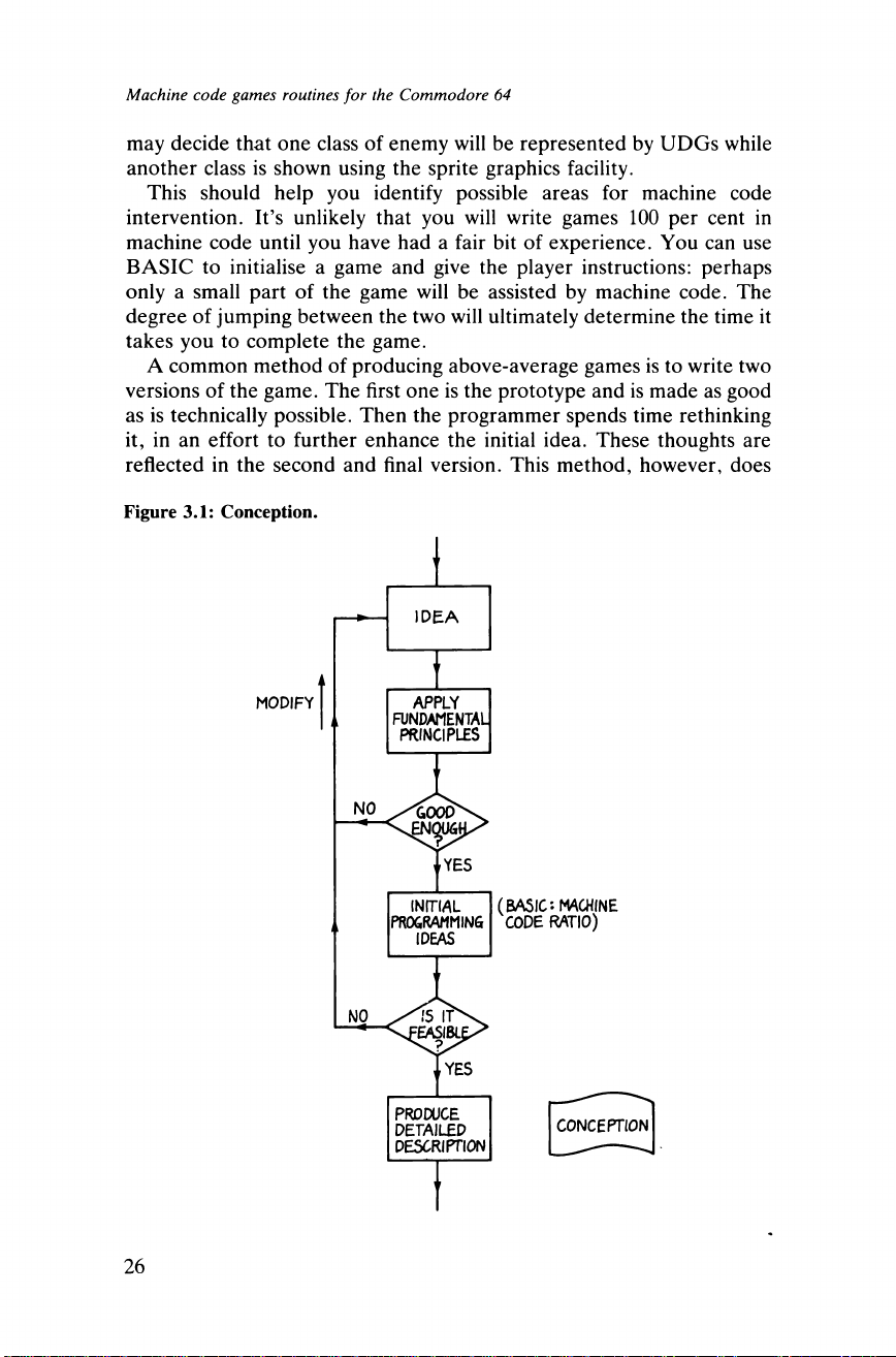
Figure 3.1: Conception.

MODIFY

(BASIC'* MACHINE

CODE RATIO)

CONCEPTION

26

Chapter 3 The Birth of a Game

have the grave disadvantage that it takes longer than ever to write the
program. This is often avoided by writing the first program totally in
BASIC and ignoring the lack of speed. At this stage (which can take

only a day or two) both the idea and the techniques involved are
developed so that the final product is as near perfect as possible. For the

absolute beginner I would advise that he (or she) refrain from this
method as it really is boring and unrewarding for the novice.

Once you think you have developed your idea in sufficient detail,
make sure that it is not ambiguous and (more importantly) that it is
presented in a tidy format for later reference. Make sure that you have
achieved what you want. In the near future you are going to put in a fair
bit of work on this program so be sure that you are going to do what you
want to do and not what you allowed yourself to be roped into. Machine
code is really a matter of stamina and achievement. If you’re not really
interested in what you are doing, then there’s no way that you will
finish, or even look like finishing, the game. You must be totally aufait
with the game all the way through to ensure its survival. If you are
confident that this stage has been satisfactorily completed then move on
to the next section, but first have a break to allow the idea to fully
mature in your mind. Whatever you do, don’t rush it.

27

CHAPTER 4

Program Design

Once the detailed description of the game has been completed, the next
stage is to draw up the charts that will divide the game into a series of
minor tasks. You may well ask how this job is to be done, but unless it
is, the game will never be completed.

In BASIC it’s possible to write programs straight off the top of your
head. In machine code the situation is different — for a lengthy
program, there is no way round this stage of detailed specification.
Indeed, even if only a section of the program is written in machine code,
I would still advise you to stick with this stage. Once you get down to it,
you will find it surprisingly simple.

There are essentially two ways of describing a process with a visual
representation: the flowchart and the top-down chart. Each has its
virtues, although the use of a flowchart is often considered bad
programming by some institutions. My system is first to take a clean
sheet of paper and write in a box at the top of the page, in the middle,
the title of the program. This is ‘very high level’: what I mean by this is
that I (the human) understand it but the computer hasn’t got the faintest
idea of what the task is. The next stage is to take this box and divide it
into a series of tasks not more in number than, say, four or five. Let us

take for example the program Space Invaders.

I would divide this into the following series of tasks:

Display title page.
Initialise for a game.
Play a game.
Inform player that game is over.

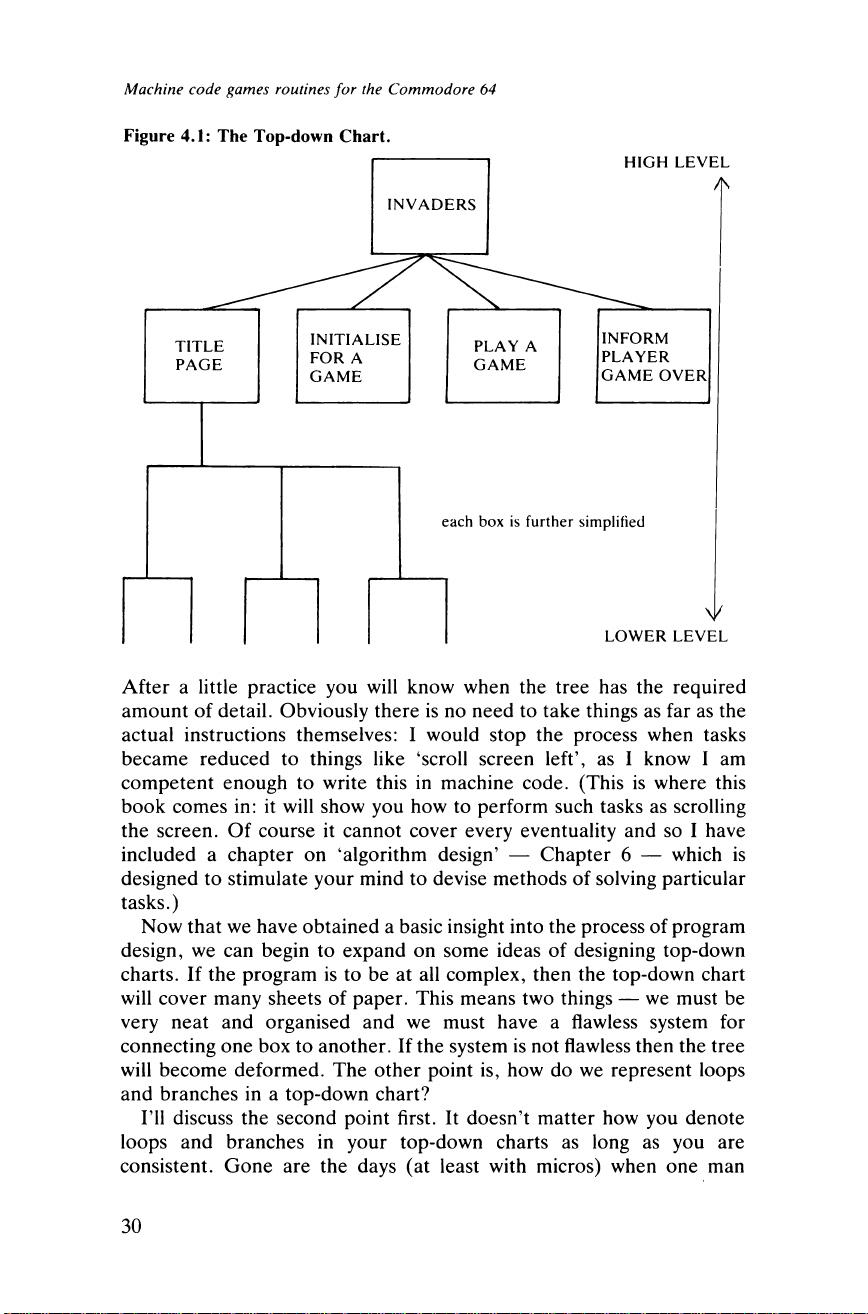
These would then be fitted into a series of boxes one row down from the
first box and connected as in Figure 4.1. Notice that the level of the
description has dropped, in that it is more ‘machine-orientated’ than the
first box. Subsequent stages simply mean taking each of these boxes and
dividing and sub-dividing it further still, until the task of encoding it is
little more than a straightforward exercise in coding. The final result will
resemble the roots of a tree. At each stage a root splits into several other

roots.

29

Machine code games routines for the Commodore 64

Figure 4.1: The Top-down Chart.

After a little practice you will know when the tree has the required

amount of detail. Obviously there is no need to take things as far as the
actual instructions themselves: I would stop the process when tasks
became reduced to things like ‘scroll screen left’, as I know I am
competent enough to write this in machine code. (This is where this
book comes in: it will show you how to perform such tasks as scrolling
the screen. Of course it cannot cover every eventuality and so I have
included a chapter on ‘algorithm design’ — Chapter 6 — which is
designed to stimulate your mind to devise methods of solving particular
tasks.)

Now that we have obtained a basic insight into the process of program
design, we can begin to expand on some ideas of designing top-down
charts. If the program is to be at all complex, then the top-down chart
will cover many sheets of paper. This means two things — we must be
very neat and organised and we must have a flawless system for
connecting one box to another. If the system is not flawless then the tree
will become deformed. The other point is, how do we represent loops
and branches in a top-down chart?

I’ll discuss the second point first. It doesn’t matter how you denote
loops and branches in your top-down charts as long as you are
consistent. Gone are the days (at least with micros) when one man

30

Chapter 4 Program Design

would describe the program and another would write it. You and you
alone are writing this program. As long as you know what you mean
then all is well. You will probably be aware of the notation used when
using flowcharts (diamond box for decisions, rectangular box for
processes, etc). A top-down notation is not normally shown by the
shape of the boxes but by signs inside each box. I will show you my
notation (which I didn’t develop) but feel free to develop your own if
you think that it’s clearer. If you are doing this, then it might be a good
idea to write down on a separate piece of paper exactly how your system
works so that you don’t deviate from it.

Figure 4.2: Top-down Schematics.

^WHAT THE BOX IS ABOUT^

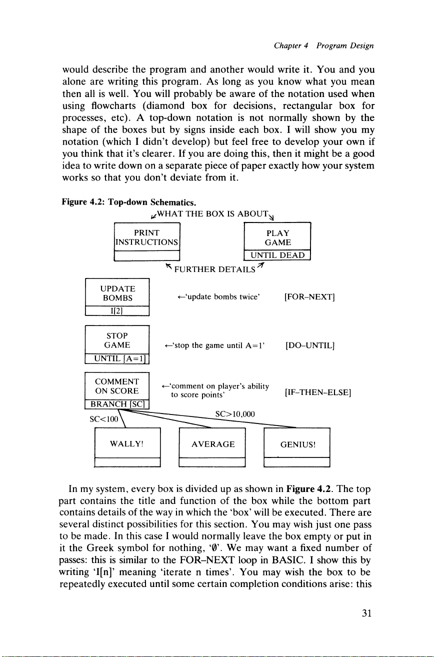
In my system, every box is divided up as shown in Figure 4.2. The top

part contains the title and function of the box while the bottom part

contains details of the way in which the ‘box’ will be executed. There are
several distinct possibilities for this section. You may wish just one pass
to be made. In this case I would normally leave the box empty or put in

it the Greek symbol for nothing, ‘0’. We may want a fixed number of
passes: this is similar to the FOR-NEXT loop in BASIC. I show this by
writing T[n]’ meaning ‘iterate n times’. You may wish the box to be

repeatedly executed until some certain completion conditions arise: this

31

Machine code games routines for the Commodore 64

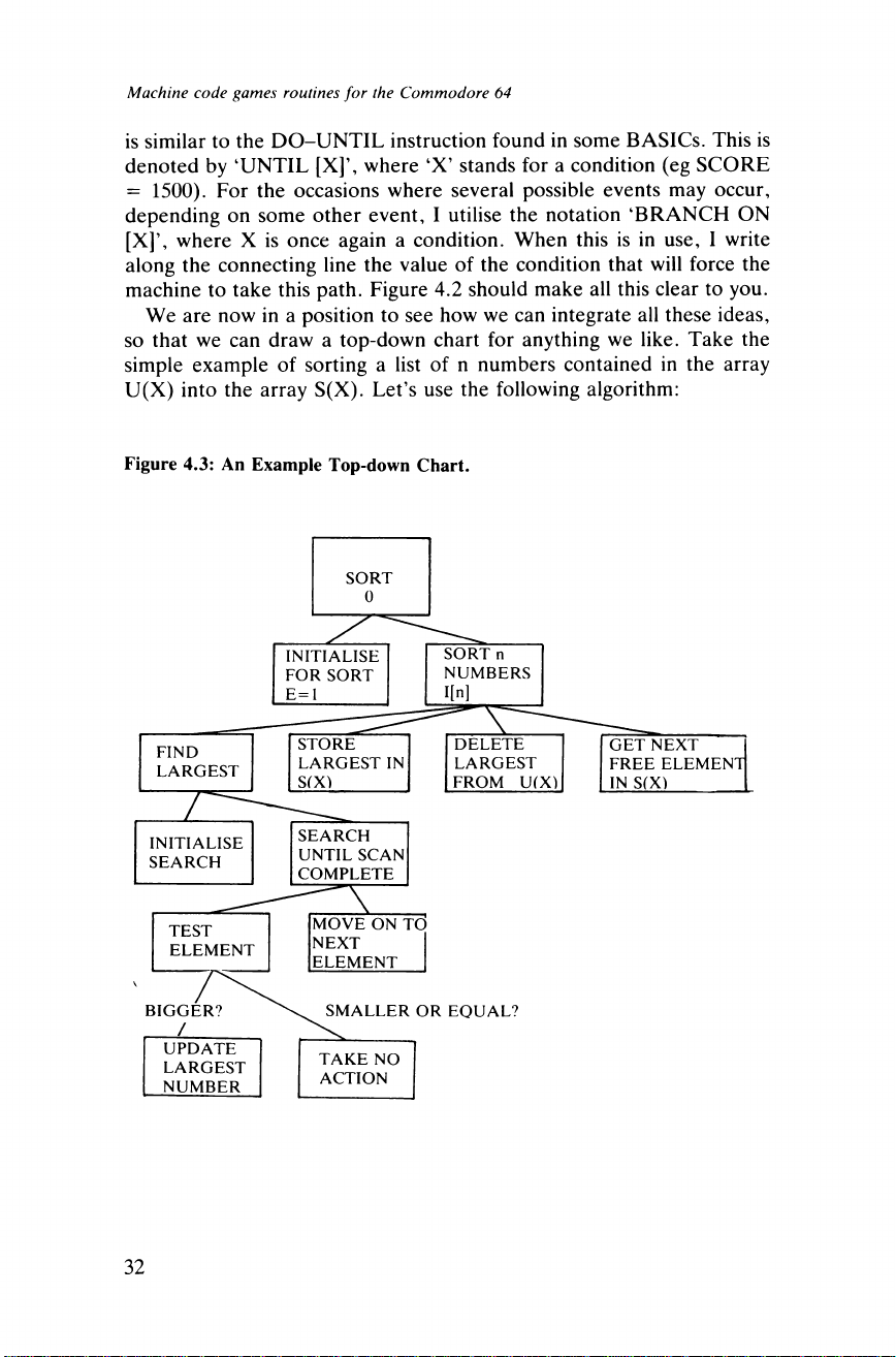
is similar to the DO-UNTIL instruction found in some BASICs. This is
denoted by ‘UNTIL [X]’, where ‘X’ stands for a condition (eg SCORE

= 1500). For the occasions where several possible events may occur,

depending on some other event, I utilise the notation ‘BRANCH ON

[X]’, where X is once again a condition. When this is in use, I write
along the connecting line the value of the condition that will force the
machine to take this path. Figure 4.2 should make all this clear to you.

We are now in a position to see how we can integrate all these ideas,
so that we can draw a top-down chart for anything we like. Take the
simple example of sorting a list of n numbers contained in the array
U(X) into the array S(X). Let’s use the following algorithm:

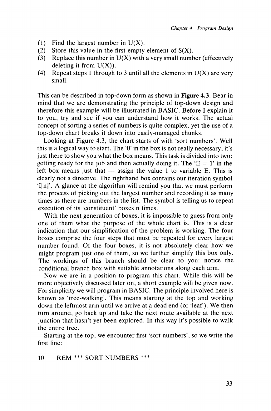
Figure 4.3: An Example Top-down Chart.

32

Chapter 4 Program Design

(1) Find the largest number in U(X).
(2) Store this value in the first empty element of S(X).
(3) Replace this number in U(X) with a very small number (effectively

deleting it from U(X)).

(4) Repeat steps 1 through to 3 until all the elements in U(X) are very

small.

This can be described in top-down form as shown in Figure 4.3. Bear in
mind that we are demonstrating the principle of top-down design and
therefore this example will be illustrated in BASIC. Before I explain it
to you, try and see if you can understand how it works. The actual
concept of sorting a series of numbers is quite complex, yet the use of a
top-down chart breaks it down into easily-managed chunks.

Looking at Figure 4.3, the chart starts of with ‘sort numbers’. Well
this is a logical way to start. The ‘O’ in the box is not really necessary, it’s
just there to show you what the box means. This task is divided into two:
getting ready for the job and then actually doing it. The ‘E = T in the
left box means just that — assign the value 1 to variable E. This is
clearly not a directive. The righthand box contains our iteration symbol
T[n]’. A glance at the algorithm will remind you that we must perform

the process of picking out the largest number and recording it as many
times as there are numbers in the list. The symbol is telling us to repeat
execution of its ‘constituent’ boxes n times.

With the next generation of boxes, it is impossible to guess from only
one of them what the purpose of the whole chart is. This is a clear
indication that our simplification of the problem is working. The four
boxes comprise the four steps that must be repeated for every largest
number found. Of the four boxes, it is not absolutely clear how we

might program just one of them, so we further simplify this box only.

The workings of this branch should be clear to you: notice the

conditional branch box with suitable annotations along each arm.

Now we are in a position to program this chart. While this will be
more objectively discussed later on, a short example will be given now.
For simplicity we will program in BASIC. The principle involved here is

known as ‘tree-walking’. This means starting at the top and working
down the leftmost arm until we arrive at a dead end (or ‘leaf’). We then
turn around, go back up and take the next route available at the next
junction that hasn’t yet been explored. In this way it’s possible to walk
the entire tree.

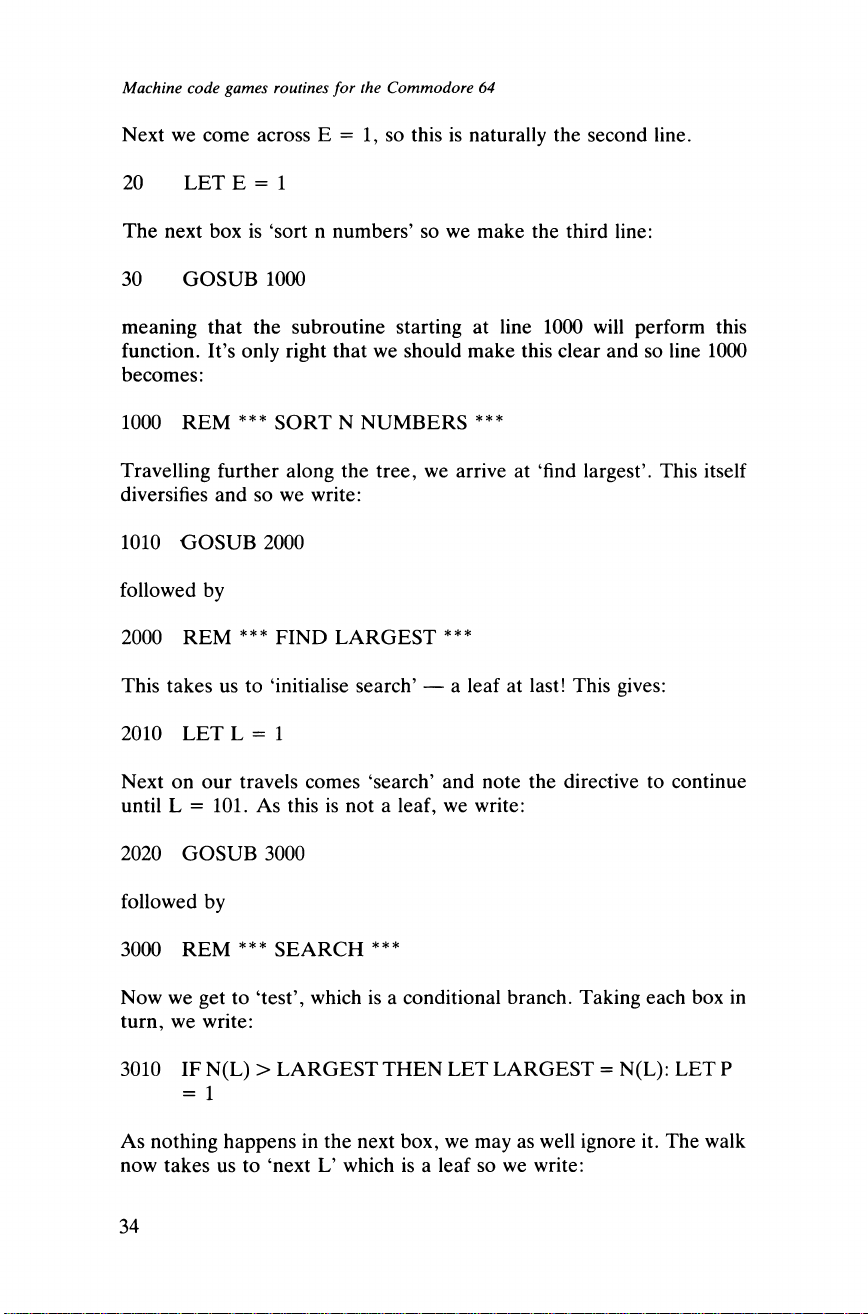
Starting at the top, we encounter first ‘sort numbers’, so we write the

first line:

10 REM *** SORT NUMBERS ***

33

Machine code games routines for the Commodore 64

Next we come across E = 1, so this is naturally the second line.

20 LET E = 1

The next box is ‘sort n numbers’ so we make the third line:

30 GOSUB 1000

meaning that the subroutine starting at line 1000 will perform this
function. It’s only right that we should make this clear and so line 1000
becomes:

1000 REM *** SORT N NUMBERS ***

Travelling further along the tree, we arrive at ‘find largest’. This itself
diversifies and so we write:

1010 GOSUB 2000

followed by

2000 REM *** FIND LARGEST ***

This takes us to ‘initialise search’ — a leaf at last! This gives:

2010 LET L = 1

Next on our travels comes ‘search’ and note the directive to continue
until L = 101. As this is not a leaf, we write:

2020 GOSUB 3000

followed by

3000 REM *** SEARCH ***

Now we get to ‘test’, which is a conditional branch. Taking each box in
turn, we write:

3010 IF N(L) > LARGEST THEN LET LARGEST = N(L): LET P

= 1

As nothing happens in the next box, we may as well ignore it. The walk
now takes us to ‘next L’ which is a leaf so we write:

34

Chapter 4 Program Design

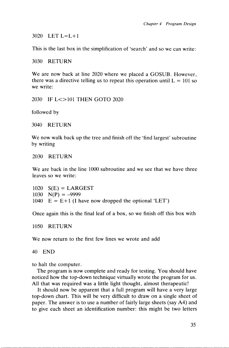
3020 LET L=L +1

This is the last box in the simplification of ‘search’ and so we can write:

3030 RETURN

We are now back at line 2020 where we placed a GOSUB. However,
there was a directive telling us to repeat this operation until L = 101 so
we write:

2030 IF LO 101 THEN GOTO 2020

followed by

3040 RETURN

We now walk back up the tree and finish off the ‘find largest’ subroutine
by writing

2030 RETURN

We are back in the line 1000 subroutine and we see that we have three

leaves so we write:

1020 S(E) = LARGEST
1030 N(P) = -9999
1040 E = E+l (I have now dropped the optional ‘LET’)

Once again this is the final leaf of a box, so we finish off this box with

1050 RETURN

We now return to the first few lines we wrote and add

40 END

to halt the computer.

The program is now complete and ready for testing. You should have
noticed how the top-down technique virtually wrote the program for us.
All that was required was a little light thought, almost therapeutic!

It should now be apparent that a full program will have a very large
top-down chart. This will be very difficult to draw on a single sheet of
paper. The answer is to use a number of fairly large sheets (say A4) and
to give each sheet an identification number: this might be two letters

35

Machine code games routines for the Commodore 64

from the game’s name plus the number of the sheet, which will help you
identify which game the chart belongs to. Thus for, say, Space Invaders
we might have SI1, SI2, SI3, and so on. The reference number of the
chart should be clearly written in a box at the top of the page. Make an
index of these reference numbers and the purpose of the chart on a
different sheet of paper, which will allow quick and easy cross
referencing. To identify each individual box on the page, use the page
code preceded by the letter ‘B’ (for box) with yet another code tagged
on to distinguish between all the other boxes on the page. If you’re
really keen, then make up another index page with all these codes on it.
All this paperwork will assist greatly in later stages of writing.

Once we have compiled a top-down chart, we are nearly in a position
to start coding: we can see exactly what is required and where.
Moreover, by looking carefully at the chart we can locate repetitions in
the code. These are obviously ideal candidates for turning into
subroutines. Yet more is done for us by the chart: it shows us how to
connect each of the parts and also the natural way to test each section as
it becomes available for integration into the rest of the program.

The efficient programmer should plan out all the work in a timetable
so that he can see exactly where he is (and whether he is on schedule).
Always allow yourself lots of time for each individual stage as machine
code is never written without the arrival of bugs. A proficient BASIC
programmer can write a full 10K program and have it in total working
order in two days, but a machine code programmer will be pushed to
write IK of usable code in a day.

The stages in producing a schedule vary from programmer to
programmer. Some programmers don’t need to use too much
organisation, but for a program in depth this can be mentally taxing.
The first stage is to look through the chart and identify all the routines.
Then, depending on how much of the program is to be in machine code,
single out all the machine code routines. Compile a list of all these
routines, including references to the chart. Now work through the chart,
estimating how long each routine will take to code and test (this comes

with experience) and, from this, organise your timetable. Obviously it is

good to get into a habit of following the schedule tightly, so be generous

with the estimates. You will have plenty of time to become a

‘speed-merchant’ later on.

Before moving on to the next chapter, try writing a few BASIC

programs with the top-down method so that you have a chance to really
appreciate the full value of the technique. This is what is known as

‘structured’ programming — the chart shows the program’s structure.

For efficiency and clarity I use a programmer’s template with all the
flowcharting symbols available, plus a pencil to rough out ideas. Once I
have produced the prototype chart, it is transferred on to a much

36

Chapter 4 Program Design

smarter piece of paper. Using a template means that you get uniform
boxes with square sides. You can either buy one or cut one out of
cardboard.

As a final note to this chapter, bear in mind that in drawing up this
chart you are laying the foundations of the game. It’s well worth the
time to build them securely, so take your time and double-check the tree
when it’s ready.

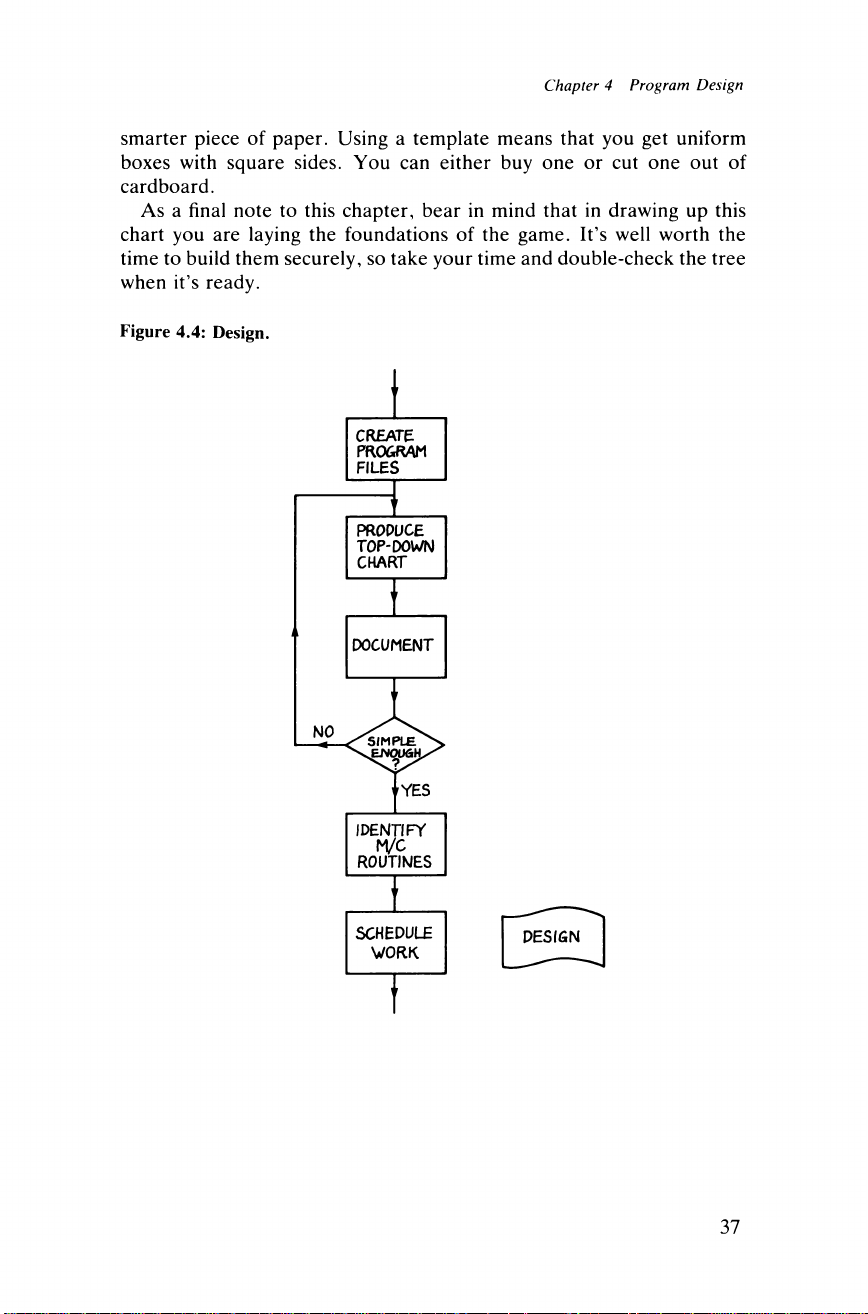
Figure 4.4: Design.

DESIGN

37

CHAPTER 5

Coding the Program

By this stage, you will have finished the groundwork and we can at last
get on with the actual writing of the program itself. Taking stock of what
has already been done, we have a detailed description of the program,
and we have also compiled the top-down charts, which tell us exactly
how to write the program. Furthermore we know which routines are to
be written in machine code and so are ready to get on with writing them.

A major part of this book is taken up with a ‘common routine’ section
(Chapters 9 and 10), which is a large selection of some of the common
routines you are likely to want to use. These range from filling areas of
memory with a code to scrolling the screen left and right (and other

directions). Each routine is discussed in terms of subject matter and
style, so that they are readily adaptable. This chapter shows you how to
use these routines to the maximum, with the minimum of work. But
don’t think that the book will write the game for you: there will be some
routines that you must construct yourself, and Chapter 6 is devoted to
this aspect.

Those of you who are alert may have noticed that there are going to
be two fundamentally different types of routine in our program. First,
there is the purely functional routine which appears at every leaf on the
top-down chart: this routine actually performs some noticeable task.
The second type of routine structures the program: it links individual
routines together and performs the inter-routine looping operations. The
latter make up each node (ie junction) of the tree. The writing of these
connecting routines is discussed in Chapter 8: the present chapter con
cerns itself with the purely functional routine only.

It is assumed that you already have a fair knowledge of machine code
in that you understand the manipulation of the registers and how to
perform the simple addition and subtraction operations which books on
6510 and 6502 code pride themselves on. As to actually writing

something worthwhile, these books (with some exceptions) tend to

leave you in the dark a little. This is because it’s very difficult to be

objective in machine code. The language lends itself very well to the
construction of short, quick, repetitive tasks, whereas the writing of a
complex program is a daunting task indeed. By the introduction of the

39

Machine code games routines for the Commodore 64

top-down chart, however, we have reduced our task into a series of very
simple sub-tasks that lend themselves well to an objective style of
programming. If this is not the case with your charts, then you simply
haven’t extended the tree in enough detail yet.

A vital instruction in machine code is the JSR/RTS combination.

These two instructions give you the capability to call subroutines just as

in BASIC. The only difference is that we can use a far higher level of
nesting than in BASIC. The 6510 allows us to use up to 128 JSR calls
without using a single RTS. This gives us the ability to call up to 127
subroutines within one subroutine. As a sneak preview of the next chap
ter, it would make sense to say that the ‘connecting routines’ work by
calling each of their subsidiary routines with JSRs. If you are not totally
clear on the topic of the JSR, go back and read up the relevant sections in
your manual.

Parameter passing

The subject of parameter passing is a vital concept. Parameters are the
pieces of information that a routine requires to do its job. The
parameters of a PRINT statement in BASIC are the variables and any
text that you wish to have printed. Consequently in machine code
various routines will need some parameters. Some, however, won’t
need any. To give an example, consider a routine that fills a section of
memory with a certain character. To perform this function the routine
must know where to start and stop filling, and also what character to fill
with. In BASIC there is only one way of parameter passing and that is to
assign the values to be passed into a variable which the routine itself
must interrogate. In machine code there are two distinct methods.
Either the values required can be dumped into some pre-determined
memory locations so that the routine can pick them up, or the data can
be put on to the stack. For our purposes, we will use the first method as
it is easier to implement.

To demonstrate this method, let’s suppose we are going to use a Fill
routine and so must pass two addresses and one code to the routine. As
long as the parameters are sent and received in the same fashion, no
problems will arise. We can store the two addresses in locations 251-252
and 253-254 as a pair of 16-digit numbers. As the code with which to fill
the area is only a single byte we could send it in the X register (no
particular choice, it could as easily have been the Y register). As long as
the Fill routine knew about this, then there would be no problems. An
important fact arises from this. If a routine is to be used with only one
set of parameters throughout the program, then it would make sense to

forget passing them at all and simply initialise them as part of the

routine itself. It is up to you to spot when this sort of situation arises and

40

Chapter 5 Coding the Program

to act accordingly.

The same sort of reasoning is true for passing parameters back from
the routine to the calling routine and then on into the next routine. This
is a topic which will be discussed later in this chapter and in Chapter 8 in
more detail, but for the time being we are ready to start looking at some of
the routines that we must encode with a view both to parameter passing
and to the actual function of the routine. Of course, there will be some
routines that don’t demand any parameters.

Compiling routines

Assuming that you are ready, we can start to compile some of the
routines. The procedure for doing this isn’t just to put pen to paper; you
will be forced to think a bit about what you are doing. The system that I
describe here shouldn’t be strictly adhered to after a while; it’s just to
point you in the right direction, to help you get started. One of the key
considerations at this stage is not to work too fast — you will not succeed,
and you will only be disappointed. Working in machine code is a slow and
laborious process: and be ready for the bugs, for they are the real test of
your stamina.

The first stage of compilation is to study the routine to be encoded.
Are you fully aware of its function? Is it simple enough to encode, or
have you failed to simplify the tree to the required extent? You must
know what you are trying to achieve right down to the last detail.
Furthermore, you must be well aware of what parameters the routine
requires.

The next stage is to try and find the corresponding ancillary routine (if
there is one). You may find an ancillary routine with a close similarity or a
very vague one to the routine for encoding. More often than not, the
encoding routine will be a hybrid of two or more of the ancillary routines.
If there is no real similarity then it looks like you are faced with the
prospect of writing the routine from scratch: put it aside for the time being
and move on to the next routine (the next chapter deals with writing from
scratch).

In order to do this speedily, you would be well advised to get to know all
of the routines fairly well, so that when you come to use one you already
have a fair amount of confidence in it. But don’t just leave it at that; make
up your own routines and document them. Then start mixing them
(mentally) and you may be amazed at some of the new routines you find
yourself with.

Study each routine and establish the parameters it needs. These fall
into two classes: in-going and out-going. In the case of in-going data, find
out which (if any) are staying constant. This information may as well be
entered by the routine itself rather than by the calling routine. All this

41

Machine code games routines for the Commodore 64

information should be carefully recorded in the program files so that it’s
available when you need it.

I must point out the danger of parameter clashes: these occur when

more than one routine uses the same memory location for a different

parameter. This results in loss of data and an erroneous entry for its

replacement. Most of the time, clashes will not matter as the
information carried in these locations won’t be needed any more, but
occasionally disaster will strike and it can be very difficult indeed to spot
the fault as the routines work on their own, but result in a bug when run
together, which is very frustrating. To prevent this, you must keep a
detailed record of what memory locations are used, and where.

If you’ve followed the instructions so far you will now be in a position

to write the routines (well, some of them, at least). Whether or not you

own an assembler, you need a copy of all the routines you write so that

these are instantly available. I would suggest copying the routines on to a

ruled page so that everything is crystal clear: you can’t afford any ambi

guity.

The first version is the prototype — just make sure it works. It doesn’t
matter if it’s a little inefficient. At this stage, you should not be using any
of the clever tricks that abound in machine code programs: keep things
plain, and try to avoid the use of JMP instructions within a routine as
these render the code un-relocatable. There should be no call to jump
further than 127 bytes, which is the limit for relative branches. To use a
conditional branch as an unconditional branch, you force the branch by
setting the flag which governs that branch. An example of this is to
precede a BCC instruction with a CLC instruction. If you are hand
assembling, then be wary of calculating these vectors as they are a
common source of error.

Once you have produced the prototype routine, assembled, tested
and corrected it, the next stage is to improve it. You may like it as it

stands or you may have noticed some improvements that you can add. If
so, go ahead by all means and change it — but don’t forget to re-test it

after the change.

42

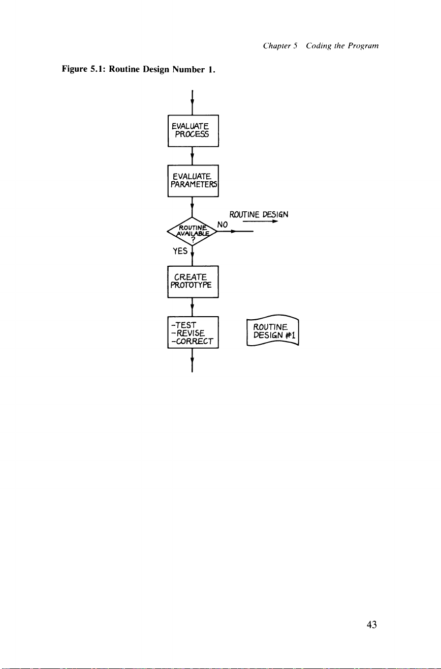
Figure 5.1: Routine Design Number 1.

Chapter 5 Coding the Program

43

CHAPTER 6

Writing Your Own Routines

Not all the routines you are going to want can be written for you. You
either have to try writing them, or shy away from machine code and
write them in BASIC. At least make an attempt at machine code: even

if you fail miserably, you will have gained valuable experience.

The first consideration is whether or not you know how to achieve
what you actually want in normal terms. Suppose you want a routine to
play chess, it's difficult enough describing the process in English, let
alone converting it into machine code. If this is the case, then what you
have is an algorithm problem — see the section on algorithm design
later in this chapter. But don’t expect instant success, inspiration may
not come at once.

Well then, assuming you have got your algorithm worked out, we can
consider turning it into an operative machine code routine. First, draw
up a flowchart of the algorithm. For planning programs as a whole the
flowchart is a poor tool, but for laying down an algorithm it is very
effective. Try to make each box as simple as possible, but there is no
need to get right down to the instructions themselves. What is wanted is
something between the two flowcharts in Figure 6.1, which add two
numbers together. Where necessary, indicate program flow lines with
arrows. Where program control can take various paths, these should be
kept to a minimum as otherwise the diagram can become cluttered. A
major cause of failure in machine code (and other computer languages)
is an over-complicated branching structure. This leads to unforeseen
logical errors, leading to a very frustrated programmer. It should be

possible to re-draw the flowchart several times, simplifying both the flow
structure and the instruction content.

By now you should be well aware of parameters to be passed to and
from the program. Note these down at the top and bottom of a sheet of
paper. From the flowchart, the main part or ‘spine’ of the routine should

be obvious. Don’t worry about the other little bits, just copy down on
the sheet the code which you think will perform this task. If you’re not
sure then type it in and check it. You will then be able to start adding in
the other ‘arms’ of the flowchart. After each stage stop and check —
don’t do it all in one go. Once this is done you have written the routine.
Look at the top and bottom of the sheet and add in the parameter
passing code. This is just the prototype — if it works, then fine, but you

45

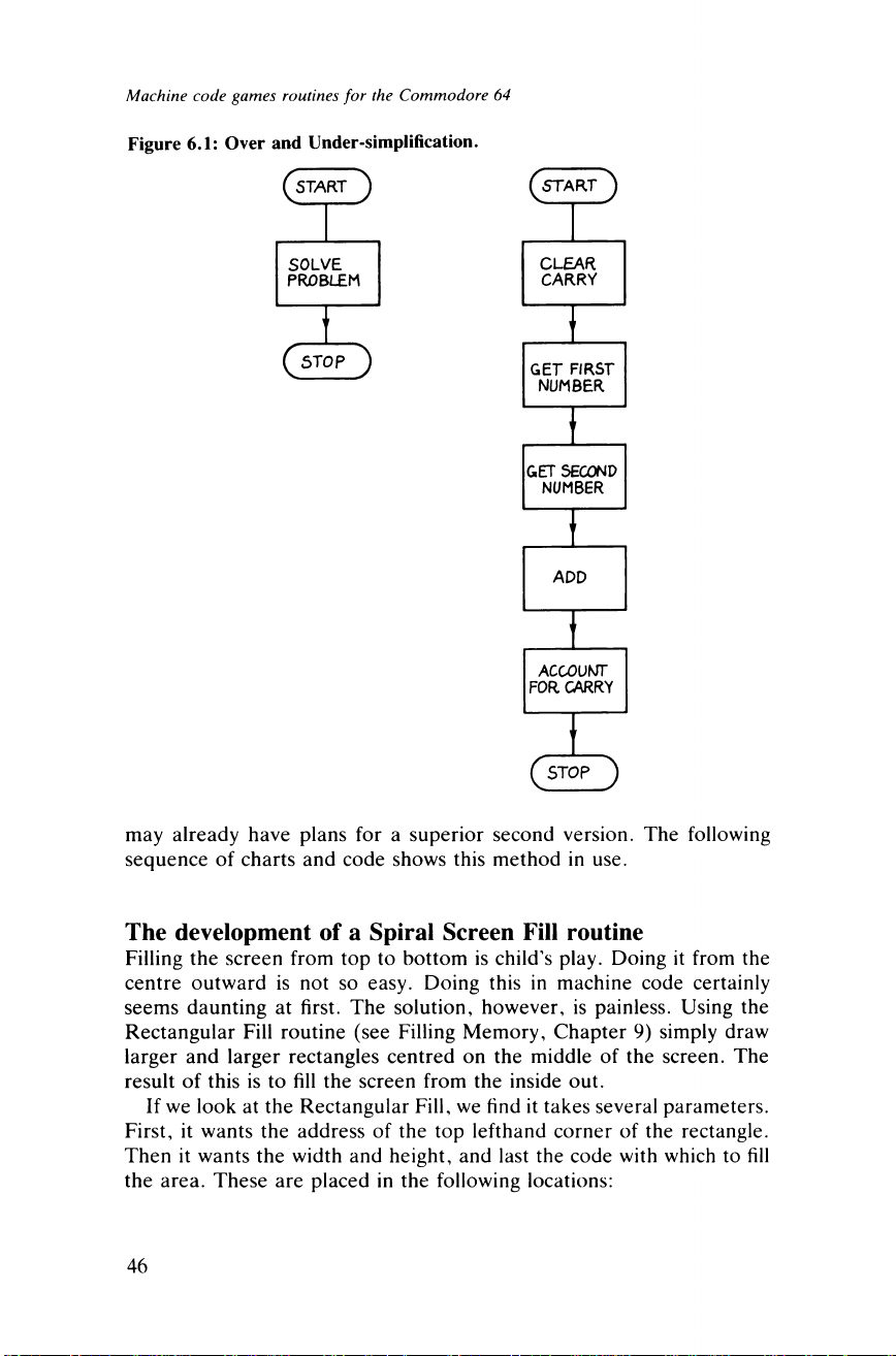
Machine code games routines for the Commodore 64

Figure 6.1: Over and Under-simplification.

may already have plans for a superior second version. The following

sequence of charts and code shows this method in use.

The development of a Spiral Screen Fill routine

Filling the screen from top to bottom is child’s play. Doing it from the

centre outward is not so easy. Doing this in machine code certainly

seems daunting at first. The solution, however, is painless. Using the

Rectangular Fill routine (see Filling Memory, Chapter 9) simply draw

larger and larger rectangles centred on the middle of the screen. The

result of this is to fill the screen from the inside out.

If we look at the Rectangular Fill, we find it takes several parameters.
First, it wants the address of the top lefthand corner of the rectangle.
Then it wants the width and height, and last the code with which to fill
the area. These are placed in the following locations:

46

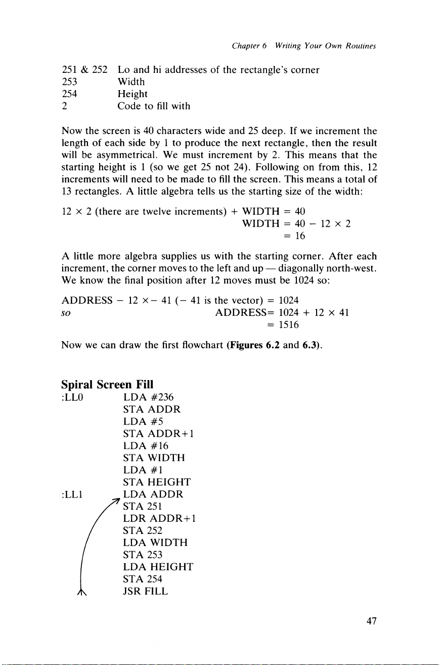
Chapter 6 Writing Your Own Routines

251 & 252 Lo and hi addresses of the rectangle’s corner

253 Width
254 Height
2 Code to fill with

Now the screen is 40 characters wide and 25 deep. If we increment the
length of each side by 1 to produce the next rectangle, then the result
will be asymmetrical. We must increment by 2. This means that the
starting height is 1 (so we get 25 not 24). Following on from this, 12
increments will need to be made to fill the screen. This means a total of

13 rectangles. A little algebra tells us the starting size of the width:

12 x 2 (there are twelve increments) + WIDTH = 40

WIDTH = 40 - 12 x 2

= 16

A little more algebra supplies us with the starting corner. After each
increment, the corner moves to the left and up — diagonally north-west.

We know the final position after 12 moves must be 1024 so:

ADDRESS - 12 x - 41 (- 41 is the vector) = 1024

so ADDRESS= 1024 + 12 x 41

= 1516

Now we can draw the first flowchart (Figures 6.2 and 6.3).

Spiral Screen Fill

:LL0 LDA #236

STA ADDR
LDA #5
STA ADDR+1
LDA #16
STA WIDTH
LDA #1
STA HEIGHT

:LL1 LDA ADDR

STA 251

/ LDR ADDR+1

/ STA 252

/ LDA WIDTH

/ STA 253

LDA HEIGHT
STA 254

/K JSR FILL

47

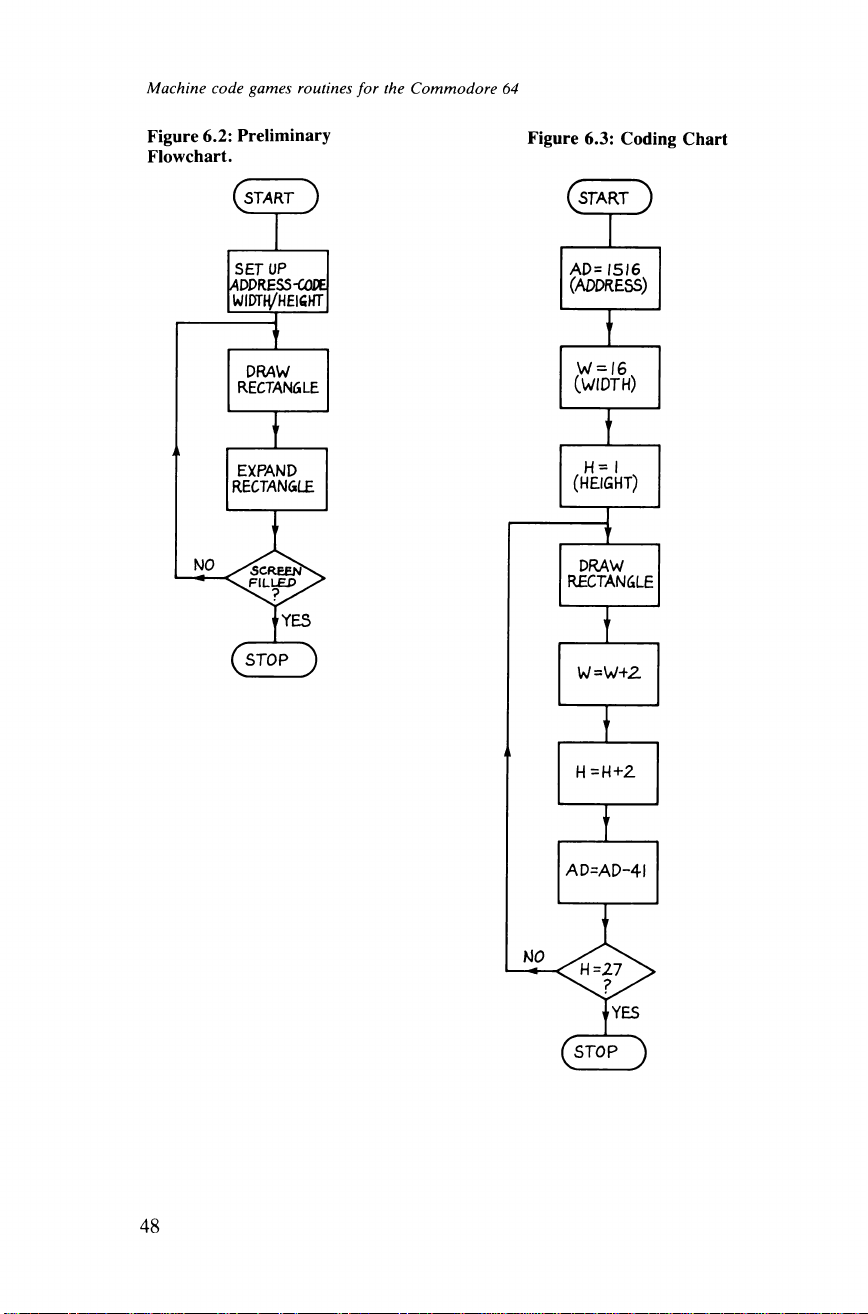
Machine code games routines for the Commodore 64

Figure 6.2: Preliminary Figure 6.3: Coding Chart
Flowchart.

48

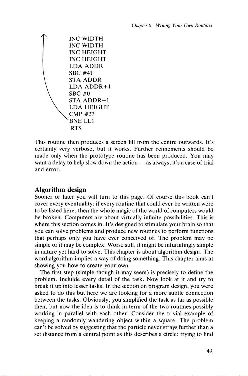
Chapter 6 Writing Your Own Routines

INC WIDTH
INC WIDTH
INC HEIGHT
INC HEIGHT
LDA ADDR
SBC #41

V

STA ADDR
LDA ADDR+1
SBC #0
STA ADDR+1
LDA HEIGHT
CMP #27
BNE LL1

RTS

This routine then produces a screen fill from the centre outwards. It’s
certainly very verbose, but it works. Further refinements should be
made only when the prototype routine has been produced. You may
want a delay to help slow down the action — as always, it’s a case of trial
and error.

Algorithm design

Sooner or later you will turn to this page. Of course this book can’t
cover every eventuality: if every routine that could ever be written were
to be listed here, then the whole magic of the world of computers would
be broken. Computers are about virtually infinite possibilities. This is
where this section comes in. It’s designed to stimulate your brain so that
you can solve problems and produce new routines to perform functions
that perhaps only you have ever conceived of. The problem may be
simple or it may be complex. Worse still, it might be infuriatingly simple
in nature yet hard to solve. This chapter is about algorithm design. The
word algorithm implies a way of doing something. This chapter aims at
showing you how to create your own.

The first step (simple though it may seem) is precisely to define the
problem. Inclulde every detail of the task. Now look at it and try to
break it up into lesser tasks. In the section on program design, you were
asked to do this but here we are looking for a more subtle connection
between the tasks. Obviously, you simplified the task as far as possible
then, but now the idea is to think in term of the two routines possibly
working in parallel with each other. Consider the trivial example of
keeping a randomly wandering object within a square. The problem
can’t be solved by suggesting that the particle never strays further than a

set distance from a central point as this describes a circle: trying to find

49

Machine code games routines for the Commodore 64

an algorithm in terms of the distance won’t work. The answer is to
consider the vertical and horizontal distances separately. Don’t expect
the answer to jump out at once. This is simply a step in the right
direction. Don’t try to solve one algorithm on its own. Do several at
once as you may find that one will help with another. The ability to think
clearly and with a very open mind are key attributes that you will gain
from algorithm design.

Once this first stage is under way (the whole thing is a dynamic
process) there are various things you can try in order to find a solution.
These are not the only methods, so don’t refrain from using your own.

One essential, however, is a doodling pad as it lets your mind wander
into wider avenues than before. The aim is to reduce the problem into a
series of clear and unambiguous stages suitable for coding (some people
tend to forget what they are aiming at). It’s important to keep the
destination in mind, so every now and again re-read the definition of the
problem.

The first thing to remember is that every problem has a solution. And
the hardest ones sometimes tend to have very elegant solutions. Just as
in the field of maths, help often comes from a section you thought had
nothing to do with the problem. Consider the problem of creating a
sense of movement into the screen (ie falling down a shaft) by drawing
perspective lines and moving them outwards, slowly at the centre and

quickly at the edges of the screen. Who would have thought that a
solution lies in the use of UDGs (see Chapter 10). This brings up

another point — there is more than one solution so don’t fall into the
trap of thinking that ‘there’s only one way to do it, and it has got
something to do with this . . .’.

Don’t be blinded by your destination. The chances are that the

solution to the problem takes an indirect route there, so don’t look for
the single-stage solution. Magazines are a good source of ideas and
programs — you’ll be surprised what you can pick up by browsing
through the listed programs and notes, which will show you how others
solve problems.

There is normally a lazy way out of algorithm solving, in that it’s

normally possible to take each instance separately and write a routine
for each. This is highly unsatisfactory but it does mean that you can get a
sort of stand-in. There are circumstances when it is a perfectly good

alternative. Take, for example, the task of providing trigonometrical
formulae in machine code for 3D perspective projection. One way is to
write floating-point routines and then use approximation formulae. This
is very clearly a daunting task. The answer is that the ratios need only be
supplied in 5° intervals anyway, and so you might as well use a table of
angles and values instead. The result? — a fast routine that’s quick and
easy to write.

50

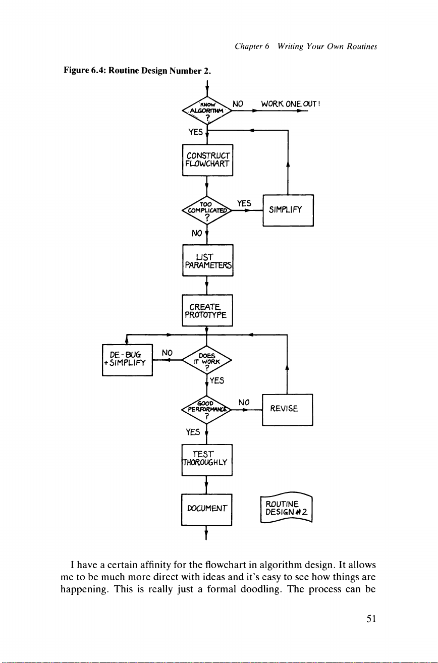
Chapter 6 Writing Your Own Routines

Figure 6.4: Routine Design Number 2.

I have a certain affinity for the flowchart in algorithm design. It allows

me to be much more direct with ideas and it’s easy to see how things are

happening. This is really just a formal doodling. The process can be

51

Machine code games routines for the Commodore 64

quite fun although if you’re not careful the diagram may get
over-complicated. But I think the flowchart ought to have a place in the
programmer’s arsenal.

Manually performing the process you are trying to devise an
algorithm for can often be enlightening. After a while you find yourself
‘doing things without thinking’. It’s at this stage that you must probe
further in and enquire what is the underlying principle. Consider the
eight queens problem:

Place eight queens on a chess-board so that no queen attacks any other.

Write an algorithm, suitable for use by a computer, to solve this
problem. The task does seem a little overpowering at first, but if you
attempt the solution manually you will find that it just takes a few
minutes to see the light.

One of my pet ways of solving problems is the approximation method.
I start off with an idea and gradually improve and refine it until I find the
answer. The initial approximation takes the form of an educated guess

at the solution and what factors may help solve it. The answer can turn
out to be totally Heath Robinson due to all the alterations but that
doesn’t really matter — as long as it’s ‘watertight’, it will work and you
can always improve on it later. Remember this is just the prototype.

These then are some of the chief methods of algorithm design. Use
them liberally and just let your mind wander. Inspiration may come to
you at the most unexpected moments. It’s unlikely that you will work
things out instantly, but then again it’s unlikely that you’ll find yourself
with too many difficult algorithms anyway. Most of the problems not
supported by the service routines supplied will yield readily to
decomposition.

52

CHAPTER 7

Testing and Debugging

No program in machine code is ever without its associated bugs. The
longer it is the worse they are, and the more numerous. It is reasonable
only to expect the shortest routines to work first time. This chapter is all
about the hunting and killing of bugs. It’s vital to remove them
completely and kill them dead. The good programmer expects bugs (but
hopes for none) and so is quite prepared to fight them.

Bugs come in all shapes, sizes and guises. They may be caused by
errors, faulty algorithms or any one of a hundred causes. There is no
such thing as the standard bug and sometimes it’s difficult to even
recognise the problem. One of the best debugging aids is the dry-run
with paper and pencil but prevention is always better than cure, which is
why this chapter comes in three sections. First how to keep your
routines simple, second how to test them and third how to debug them.
This chapter is possibly the most valuable in the whole book as it only
takes a few bugs for you to lose heart and give up. Stand up and fight

them: after all, if machine code programming was simple you wouldn’t
get so much satisfaction out of it. Trouble-shooting a program can even
be fun if you enter into it in the right spirit.

Keeping routines simple

A simple routine is a programmer’s dream. All you have to do is keep it
short and straightforward — no clever tricks. There should be as few
branches as possible to minimise the total number of different paths.
Don’t hesitate to use a JSR in a routine even if this is the only time that
routine is called. If the routine is therefore simpler, then the JSR is
doing its job. Ideally a routine should be no more than, say, 25
instructions. This is so that it can all fit on the screen in one go. Any
more than this, and start thinking about some JSRs.

Writing a program off the top of your head has a noticeably cramping
effect on your thought processes — even in BASIC — as you can see
only 25 lines at once. It’s far easier to work from a paper listing than a
screen — you can see the whole program at once. If you look at some of
the routines in this book you will notice that they are kept short and

53

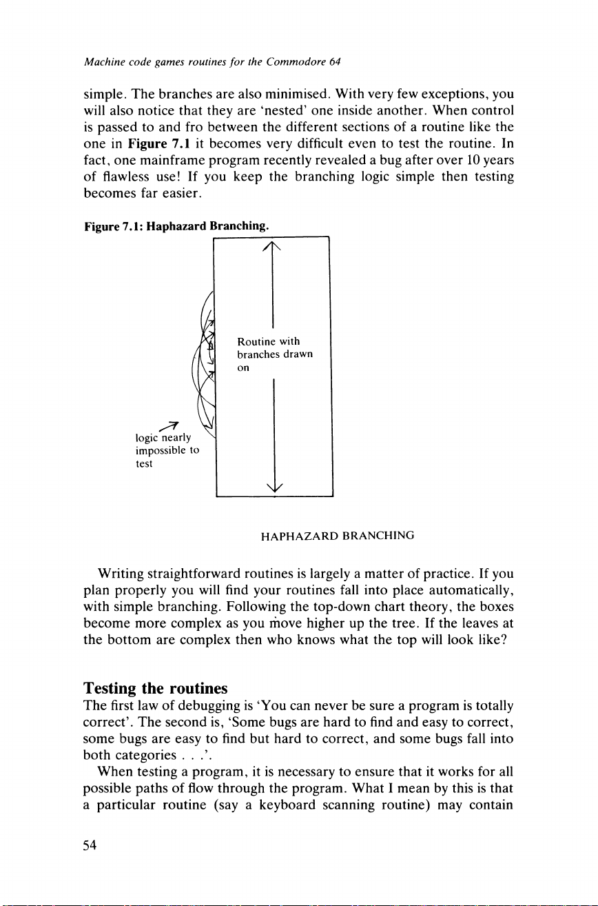
Machine code games routines for the Commodore 64

simple. The branches are also minimised. With very few exceptions, you

will also notice that they are ‘nested’ one inside another. When control

is passed to and fro between the different sections of a routine like the

one in Figure 7.1 it becomes very difficult even to test the routine. In
fact, one mainframe program recently revealed a bug after over 10 years
of flawless use! If you keep the branching logic simple then testing
becomes far easier.

Figure 7.1: Haphazard Branching.

HAPHAZARD BRANCHING

Writing straightforward routines is largely a matter of practice. If you
plan properly you will find your routines fall into place automatically,
with simple branching. Following the top-down chart theory, the boxes
become more complex as you move higher up the tree. If the leaves at
the bottom are complex then who knows what the top will look like?

Testing the routines

The first law of debugging is ‘You can never be sure a program is totally
correct’. The second is, ‘Some bugs are hard to find and easy to correct,
some bugs are easy to find but hard to correct, and some bugs fall into
both categories . . .’.

When testing a program, it is necessary to ensure that it works for all
possible paths of flow through the program. What I mean by this is that
a particular routine (say a keyboard scanning routine) may contain

54

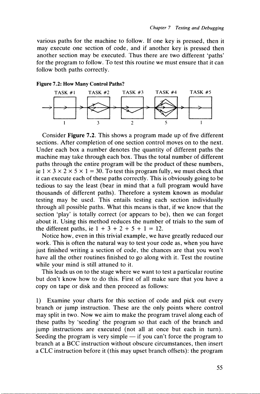
Chapter 7 Testing and Debugging

various paths for the machine to follow. If one key is pressed, then it
may execute one section of code, and if another key is pressed then

another section may be executed. Thus there are two different ‘paths’
for the program to follow. To test this routine we must ensure that it can
follow both paths correctly.

Figure 7.2: How Many Control Paths?

TASK #1 TASK #2 TASK #3 TASK #4 TASK #5

> \

1 3 2 5 1

Consider Figure 7.2. This shows a program made up of five different
sections. After completion of one section control moves on to the next.
Under each box a number denotes the quantity of different paths the
machine may take through each box. Thus the total number of different
paths through the entire program will be the product of these numbers,
ie 1 x 3 x 2 x 5 x 1 = 30. To test this program fully, we must check that
it can execute each of these paths correctly. This is obviously going to be

tedious to say the least (bear in mind that a full program would have
thousands of different paths). Therefore a system known as modular

testing may be used. This entails testing each section individually
through all possible paths. What this means is that, if we know that the
section ‘play’ is totally correct (or appears to be), then we can forget
about it. Using this method reduces the number of trials to the sum of
the different paths, iel+3 + 2T5Tl = 12.

Notice how, even in this trivial example, we have greatly reduced our
work. This is often the natural way to test your code as, when you have
just finished writing a section of code, the chances are that you won’t

have all the other routines finished to go along with it. Test the routine

while your mind is still attuned to it.

This leads us on to the stage where we want to test a particular routine
but don’t know how to do this. First of all make sure that you have a
copy on tape or disk and then proceed as follows:

1) Examine your charts for this section of code and pick out every
branch or jump instruction. These are the only points where control
may split in two. Now we aim to make the program travel along each of
these paths by ‘seeding’ the program so that each of the branch and
jump instructions are executed (not all at once but each in turn).
Seeding the program is very simple — if you can’t force the program to
branch at a BCC instruction without obscure circumstances, then insert
a CLC instruction before it (this may upset branch offsets): the program

55

Machine code games routines for the Commodore 64

will not know the difference. This method may be a bit ugly but it works
— don’t forget to remove the ‘seed’ after use. What this first stage has
done is to show that all lines of control are operative.

2) The next stage is tougher on the program. The aim here is to

confuse the routine by deliberately giving it foul data, such as it might

receive while the program is running. It is up to you to be ruthless here.

Often the programmer is well aware of an error in his thinking but
pretends that it is not present. Confronted with this type of situation you
must go back and correct your mistake as it will only return to haunt you

later on.

If your routine comes through with flying colours, then congratulations!

If, however, a bug rears its head then it is imperative that you debug the

routine before continuing. Remember one thing — the computer

doesn’t make mistakes. If something doesn’t work then it’s your fault.

Many’s the time I have seen programmers notice an error and pretend

that it’s the machine’s fault. Often a bug doesn’t appear every time a

program is run: if a bug appears and then hides for a while, don’t fall

into the trap of thinking that it really was the computer’s fault. The rule

is that if you see a bug once, then it exists and no amount of ignoring it
will get rid of it. Once you admit that there is a bug in your code you’re

half-way to correcting it.

Debugging

So now you have a bug and you know roughly where it is. You may even
have an inkling as to its cause. Apart from giving in to the pest, you have
three options: you can correct the bug; you can rewrite the faulty
section; or you can decide that the bug adds a new dimension to the
game, as in, ‘Avoid the white blobs on the screen as they are spiral
vortices which if hit cause time to stop and the game ends’, ie the
machine hangs up. (OK this is taking it a bit far but you would be
amazed at the number of programs which have been aided through
divine intervention like this. You have probably done it yourself and,
while you should guard against doing it too often, there are occasions
when bugs fit the bill perfectly.) To give this underhand system a more
technical name use the phrase ‘If it doesn’t work then document it (but
don’t tell anybody)’.

The favoured method is, of course, to correct the bug. However you
may not be able to track it down. Worse still, you may have tracked it
down but know that fixing it isn’t going to be easy. It is at this (later)
stage that you should resort to rewriting the code.

The first stage of debugging is to check that what you have entered on

56

Chapter 7 Testing and Debugging

the computer agrees with what you wanted to enter. A bug arising from
a typing error or misprint is a gremlin (merely a distant cousin of the
bug). Make sure you do this first, as otherwise you may tamper with the

code and only later discover the misprint — a sheer waste of time.

The next step in debugging is to ask the question, ‘Does it hang up?’ If
the routine goes into a loop then one of two things is probably
happening. First, check all the branch instructions, both conditional and
unconditional, as it is through these that the program can go into a loop.
Often you will find that you have miscalculated a relative branch vector.
If the code is all correct, then the next most likely cause is that
‘completion conditions’ are not occurring. Every section of code will
exit the routine when the job is done. This is where the completion
conditions come in: they inform the routine when the job is done. If
completion conditions are not occurring then there is probably a small
oversight in your code (ie the algorithm is probably correct) so the best
solution here would be to dry-run the code with a pencil and paper and
the error will give in without too much of a fight. If you find that your

code still hangs up and neither of these explanations is the right one,
then re-check the code with a fine-tooth comb: the error is in there

somewhere. You will probably be best off with a dry-run as above. It’s
only a matter of perseverance, that’s what makes the machine code

programmer.

If however your code doesn’t hang up but flatly refuses to work, then
there is an error in your algorithmic reasoning. Just in case this isn’t
true, check the code for gremlins again and be especially careful over

what addressing modes you wanted to use and what addressing modes
you actually used. If all this is done and you still can’t see the fault,
then it’s time to use some diagnostic aids. These will allow you to
follow the program flow closely which, with luck, will enlighten you.
There are a number of different aids so I would advise you to get to
know them now, so that you are aware of the aid that will assist you
most in your plight.

The first is a technique used on much larger computers. It involves
listening to the noise the processor is making (ICL machines are fitted
with a ‘Hoot Volume’ knob). On a mainframe this is detected and
amplified so that the engineers can listen to the machine’s activity. On
the 64 this noise can be heard on the TV. All you have to do is turn up
the volume and listen. Of course if you are using the SID then you won’t
be able to hear the ‘hoot’. With the volume on, listen to the noise. Now
enter this line of BASIC:

FOR A=1 TO 3000:NEXT

and press return. Hear the difference? This is the noise the machine

57

Machine code games routines for the Commodore 64

makes when in a loop. Of couse the note you hear depends on the
rapidity of execution. Thus by turning up the ‘hoot volume’ you can
listen in to the processor.

The second technique is a form of flagging. If your code is concerned

with on-screen activity then, in order for you to see what’s happening, it

may be necessary for you to insert a delay into the main loop. This is
easily done by use of the JSR instruction. Simply insert JSR (address of
delay) into the loop and run the code. For details of how to write a
delay, see the section in Chapter 9.

However, just slowing down the code may not be enough. You may
wish to see exactly the value of a register or just how far across the
screen a pointer has got. This is easily achieved by POKEing the

information on the screen before the delay and then removing it
afterwards. To show how far across the screen a pointer has got, I would
advise POKEing the address it holds with a 160 (white square) and then
removing this after the delay. When run, a white square will zip across
the screen. If you want the value of a register, then use the absolute X or
Y mode coupled with a base address of 1024. Once again, POKE a
white square on before the delay and remove it. Thus the value of the
register can be gleaned from the position of the white square. If the
square is in the top lefthand corner of the screen then the register has
value 0; the top righthand corner makes it value 39, and so on.

A far more elegant way of ascertaining register values is to use the
neglected BRK instruction. This is a software-called interrupt and is
non-maskable so you can be sure it works. Its use is simple: you simply
sprinkle BRKs liberally throughout your program and, when encoun
tered, they force an interrupt. The vector is contained at 790 and 791.
On older CBM machines the BRK instruction traditionally pointed to
the machine code monitor, but on the 64 there is no resident monitor so
we aren’t going to lose a lot. We can work the service routine two ways.
We can store register values safely somewhere and then return to
BASIC, or we can test for the function keys being depressed and act
accordingly. If no key is held down then the program continues as
normal: FI slows the program down, F2 stops it, etc. All this is dealt

with in the section on the interrupt and the Mini-toolkit in Appendix B.

For the moment we shall limit ourselves to the former option.

:LL0 ST A 820

STX 821
STY 822
JSR 58251 (return to BASIC)

Site this routine somewhere, say 49152, and alter the BRK vector to the
new address. On returning to BASIC you can discover register values by

58

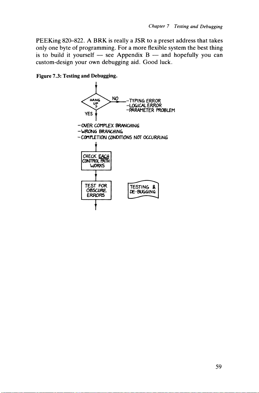
Chapter 7 Testing and Debugging

PEEKing 820-822. A BRK is really a JSR to a preset address that takes
only one byte of programming. For a more flexible system the best thing
is to build it yourself — see Appendix B — and hopefully you can
custom-design your own debugging aid. Good luck.

Figure 7.3: Testing and Debugging.

-T Y P ING ERROR

-LOGICAL ERROR

-PARA METER PROBLEM

-OVER COMPLEX BRANCHING

-VJ^ONtk BRANCHING

-COMPLETION CONDm ONS NOT OCCURRING

TESTING &
OE-BUGGING

59

CHAPTER 8

Connections: Stringing the Game

Together

After you have completed a number of functional routines you will
notice that you are in a position to combine them. You can see this by

looking at the top-down chart you drew earlier on. Only the leaves (final
boxes) on the tree actually do something. All the other boxes simply
connect them together in the desired structure. Once you have
completed enough routines start connecting them, but only after they
have been thoroughly checked and tested. If this hasn’t been done,
when a bug arises you won’t know where to look. If you have checked
that the individual routines do work, however, then you know that a bug
is caused either by a parameter problem or by a faulty connection.

The first move is to look up the box on the tree and find out what
connections must be made. Check each of the routines and see what
information is passed to and from them. Check that the routines don’t
clash with each other. If problems do arise then you can either modify
(and retest) the functional routines or patch up the fault in the
connector. You should really have been aware of clashes when writing
the routines anyway — that was why I emphasised the research into the
exact function and nature of each routine.

Don’t forget that further up the tree an old result (a parameter or data
generated some time ago) may be called in for use. As long as you’re
aware of this then it’s OK. Talking about moving further on up the tree,
the connector box may not be a simple connection. It could require
iteration or conditional branching or even a DO-UNTIL loop. This
section will describe how to produce these constructs. Of course the first
part is the one-pass connection. This simply entails each routine being
called in turn: the connecting routine then returns to where it was called

from.

Each routine is called with a JSR. Any parameters should be set up

before this and afterwards a bit of tidying up may be necessary to

prepare for the next JSR. At the end of the routine you store away any
data needed in the future and then finish with an RTS. If some of the
routines are simply one-offs, then you may already have written
parameters into them. This is far preferable, as it improves the
readability of the program. For instance:

61

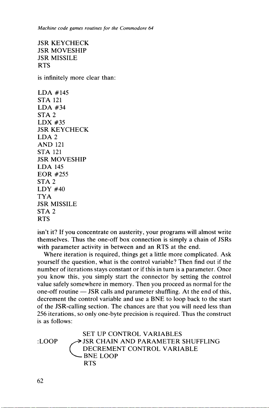
Machine code games routines for the Commodore 64

JSR KEYCHECK
JSR MOVESHIP
JSR MISSILE

RTS

is infinitely more clear than:

LDA #145

STA 121

LDA #34

STA 2

LDX #35
JSR KEYCHECK

LDA 2
AND 121
STA 121
JSR MOVESHIP
LDA 145
EOR #255
STA 2
LDY #40
TYA
JSR MISSILE
STA 2
RTS

isn’t it? If you concentrate on austerity, your programs will almost write
themselves. Thus the one-off box connection is simply a chain of JSRs
with parameter activity in between and an RTS at the end.

Where iteration is required, things get a little more complicated. Ask
yourself the question, what is the control variable? Then find out if the
number of iterations stays constant or if this in turn is a parameter. Once
you know this, you simply start the connector by setting the control

value safely somewhere in memory. Then you proceed as normal for the
one-off routine — JSR calls and parameter shuffling. At the end of this,
decrement the control variable and use a BNE to loop back to the start
of the JSR-calling section. The chances are that you will need less than
256 iterations, so only one-byte precision is required. Thus the construct
is as follows:

:LOOP

C

SET UP CONTROL VARIABLES
JSR CHAIN AND PARAMETER SHUFFLING
DECREMENT CONTROL VARIABLE

BNE LOOP
RTS

62

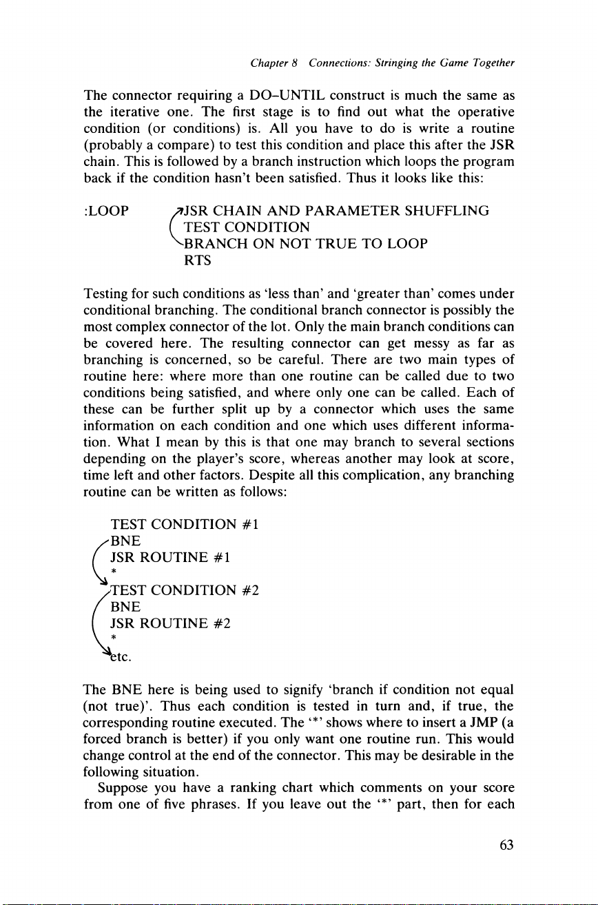
Chapter 8 Connections: Stringing the Game Together

The connector requiring a DO-UNTIL construct is much the same as

the iterative one. The first stage is to find out what the operative
condition (or conditions) is. All you have to do is write a routine
(probably a compare) to test this condition and place this after the JSR

chain. This is followed by a branch instruction which loops the program

back if the condition hasn’t been satisfied. Thus it looks like this:

:LOOP ^JSR CHAIN AND PARAMETER SHUFFLING

( TEST CONDITION

^BRANCH ON NOT TRUE TO LOOP

RTS

Testing for such conditions as ‘less than’ and ‘greater than’ comes under
conditional branching. The conditional branch connector is possibly the
most complex connector of the lot. Only the main branch conditions can
be covered here. The resulting connector can get messy as far as
branching is concerned, so be careful. There are two main types of
routine here: where more than one routine can be called due to two
conditions being satisfied, and where only one can be called. Each of
these can be further split up by a connector which uses the same
information on each condition and one which uses different informa
tion. What I mean by this is that one may branch to several sections
depending on the player’s score, whereas another may look at score,
time left and other factors. Despite all this complication, any branching
routine can be written as follows:

TEST CONDITION #1

'BNE

JSR ROUTINE #1

TEST CONDITION #2

BNE
JSR ROUTINE #2

tC.

The BNE here is being used to signify ‘branch if condition not equal

(not true)’. Thus each condition is tested in turn and, if true, the

corresponding routine executed. The ‘*’ shows where to insert a JMP (a

forced branch is better) if you only want one routine run. This would
change control at the end of the connector. This may be desirable in the
following situation.

Suppose you have a ranking chart which comments on your score

from one of five phrases. If you leave out the ‘*’ part, then for each

63

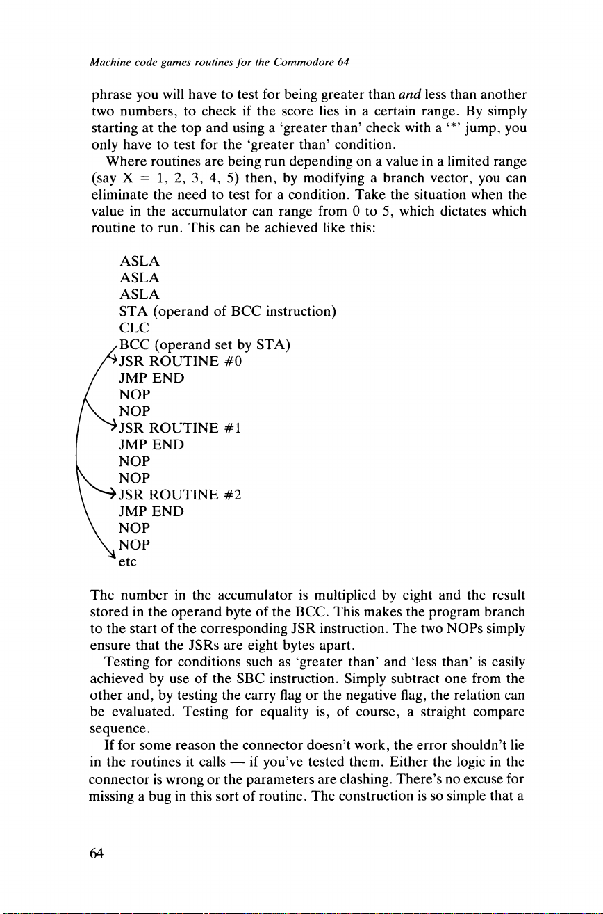
Machine code games routines for the Commodore 64

phrase you will have to test for being greater than and less than another
two numbers, to check if the score lies in a certain range. By simply
starting at the top and using a ‘greater than’ check with a ‘*’ jump, you
only have to test for the ‘greater than’ condition.

Where routines are being run depending on a value in a limited range
(say X = 1, 2, 3, 4, 5) then, by modifying a branch vector, you can
eliminate the need to test for a condition. Take the situation when the
value in the accumulator can range from 0 to 5, which dictates which
routine to run. This can be achieved like this:

ASLA
ASLA
ASLA
STA (operand of BCC instruction)
CLC

✓ BCC (operand set by STA)

A jsr ROUTINE #0

/ JMP END

/ NOP

/V NOP

^ J S R ROUTINE #1

JMP END
NOP
NOP

►JSR ROUTINE #2

JMP END
NOP
NOP
etc

The number in the accumulator is multiplied by eight and the result
stored in the operand byte of the BCC. This makes the program branch
to the start of the corresponding JSR instruction. The two NOPs simply
ensure that the JSRs are eight bytes apart.

Testing for conditions such as ‘greater than’ and ‘less than’ is easily
achieved by use of the SBC instruction. Simply subtract one from the
other and, by testing the carry flag or the negative flag, the relation can
be evaluated. Testing for equality is, of course, a straight compare
sequence.

If for some reason the connector doesn’t work, the error shouldn’t lie
in the routines it calls — if you’ve tested them. Either the logic in the

connector is wrong or the parameters are clashing. There’s no excuse for
missing a bug in this sort of routine. The construction is so simple that a

64

Chapter 8 Connections: Stringing the Game Together

dry-run to keep track of parameter addresses should show the bug up
fairly quickly. Once it works, don’t forget to document the routine —
it’s going to be used later on when you’ve forgotten all about writing it.

65

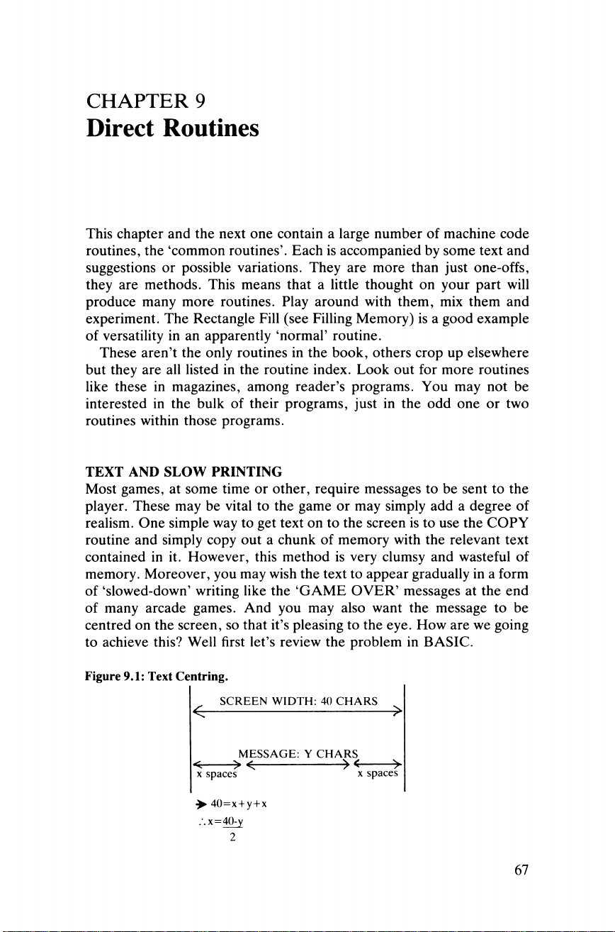
CHAPTER 9

Direct Routines

This chapter and the next one contain a large number of machine code
routines, the ‘common routines’. Each is accompanied by some text and
suggestions or possible variations. They are more than just one-offs,
they are methods. This means that a little thought on your part will
produce many more routines. Play around with them, mix them and
experiment. The Rectangle Fill (see Filling Memory) is a good example
of versatility in an apparently ‘normal’ routine.

These aren’t the only routines in the book, others crop up elsewhere
but they are all listed in the routine index. Look out for more routines
like these in magazines, among reader’s programs. You may not be
interested in the bulk of their programs, just in the odd one or two
routines within those programs.

TEXT AND SLOW PRINTING
Most games, at some time or other, require messages to be sent to the
player. These may be vital to the game or may simply add a degree of
realism. One simple way to get text on to the screen is to use the COPY
routine and simply copy out a chunk of memory with the relevant text
contained in it. However, this method is very clumsy and wasteful of
memory. Moreover, you may wish the text to appear gradually in a form
of ‘slowed-down’ writing like the ‘GAME OVER’ messages at the end
of many arcade games. And you may also want the message to be
centred on the screen, so that it’s pleasing to the eye. How are we going
to achieve this? Well first let’s review the problem in BASIC.

Figure 9.1: Text Centring.

^ SCREEN WIDTH: 40 CHARS

MESSAGE: Y CHARS

<

---------

> <;------------------------><

---------

>

x spaces x spaces

> 40=x + y + x

x=40-y

2

67

Machine code games routines for the Commodore 64

Let’s say the message is contained in M$. Let’s also assume that the
cursor is already on the right line and all we have to do is slowly print
out M$ along the centre of this line. The screen is 40 characters wide

(Figure 9.1) and the length of M$ can be determined by LEN (M$). If

the message is to appear centrally, then there must be the same number
of spaces on the line before it, as after it. If we call this ‘x’ spaces, then
we will see from the diagram that

2x + LEN (M$) = 40

Solving for x gives us

x = (40—LEN(M$) -r 2)

Thus the statement ‘PRINT TAB (x);’ will put the cursor in the position
ready for printing, and the will hold it there. Now all we have to do is
PRINT each character in turn, using the MID$ command, and
introduce a delay between each character. Try the following:

FOR C = 1 TO LEN (M$)
PRINT MID$(M$,C,1);
FOR DE=1 TO 100 : NEXT DE
NEXT C
PRINT

Don’t forget the final PRINT, as otherwise the cursor will be left
hanging after the last character of the message.

Slow printing

So that’s how we do it in BASIC. In machine code, the message is

simply a string of bytes terminated by a byte with a predetermined value

(such as 255), where each byte represents the ASCII code of that

character. Printing the characters is easy. All you do is set up a loop to
read the data in sequence (ie put the value into the accumulator) and
then call one of the ROM routines which prints a single character. To

align the cursor to the correct position beforehand, call this character
printing routine with some cursor controls (eg Home, cursor down x 5,
cursor across Xl5). Make sure that you are writing to the screen by
calling the routine to clear all I/O channels, as otherwise you may find
yourself dumping characters to the printer! A call to a delay routine
while in the main loop will slow the process down so that the human eye
can follow the process. Remember, messages of this sort are very good
for breaking up the player’s rhythm. Data input to this routine is: the

68

Chapter 9 Direct Routines

address of the text file, the text file itself and the duration of the delay
(although this may already have been set). If you have a number of
different messages, then it might be easier to have the slow printing
routine called by, say, four or five subsidiary routines which set up the

particular parameters for one message (they should also position the

cursor). Then, when you want to print out a message, all you need do is
make a call to one of the subsidiary routines. The routine returns
nothing to the caller.

Here are the addresses of the ROM routines which I referred to:

CHROUT: This outputs to a device (in our case the screen) the

ASCII character represented by the value in the
accumulator. Its address is 65490 ($FFD2).

CLRCHIN: This restores all I/O channels to normal and means that,

when CHROUT is used, the characters will go to the
screen. Its address is 65484 ($FFCC).

Variations on this theme of printing characters might be to print a space
between each character, thus ‘expanding’ the text and making it appear
larger than it actually is. Compare the following:

GAME OVER GAME OVER

The second example is novel and therefore more pleasing, but don’t
overdo it. Other ideas might be to underline the message or, best of all,
print it from the middle out. This is known as ‘meta-printing’ and can be

very effective but it’s a special effect so keep it for special things.

Meta-printing (BASIC listing)

10 L=LEN (M$) : IF L/2 = INT (L/2) THEN M$ = M$ + “ ” : L =

L+ 1
20 X = INT ((40 - L)/2)
30 FOR P = (INT (L/2) + 1) TO 1 STEP -1
40 PRINT “[CU]” TAB (X + P - 1) MID$ (M$, P, ((INT (L/2) + 1)

- P) * 2 + 1

50 NEXTP

This takes M$ and prints it from the centre outwards in the middle of a

line.

The following routine prints out the message held in ASCII form
starting at START and finishing with an entry of 13. The maximum
length is 255 bytes:

69

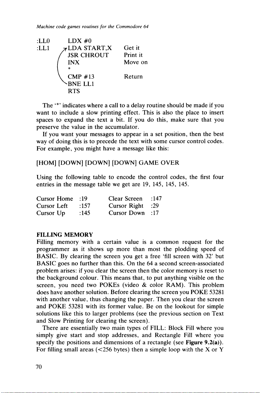
Machine code games routines for the Commodore 64

:LLO LDX #0
:LL1 LDA START,X

Get it
Print it
Move on

JSR CHROUT
INX

CMP #13

Return

X BNE LL1

RTS

The indicates where a call to a delay routine should be made if you
want to include a slow printing effect. This is also the place to insert
spaces to expand the text a bit. If you do this, make sure that you
preserve the value in the accumulator.

If you want your messages to appear in a set position, then the best

way of doing this is to precede the text with some cursor control codes.

For example, you might have a message like this:

[HOM] [DOWN] [DOWN] [DOWN] GAME OVER

Using the following table to encode the control codes, the first four

entries in the message table we get are 19, 145, 145, 145.

Cursor Home : 19 Clear Screen : 147
Cursor Left : 157 Cursor Right :29
Cursor Up : 145 Cursor Down : 17

FILLING MEMORY
Filling memory with a certain value is a common request for the
programmer as it shows up more than most the plodding speed of
BASIC. By clearing the screen you get a free ‘fill screen with 32’ but
BASIC goes no further than this. On the 64 a second screen-associated
problem arises: if you clear the screen then the color memory is reset to
the background colour. This means that, to put anything visible on the
screen, you need two POKEs (video & color RAM). This problem

does have another solution. Before clearing the screen you POKE 53281
with another value, thus changing the paper. Then you clear the screen
and POKE 53281 with its former value. Be on the lookout for simple
solutions like this to larger problems (see the previous section on Text
and Slow Printing for clearing the screen).

There are essentially two main types of FILL: Block Fill where you
simply give start and stop addresses, and Rectangle Fill where you
specify the positions and dimensions of a rectangle (see Figure 9.2(a)).
For filling small areas (<256 bytes) then a simple loop with the X or Y

70

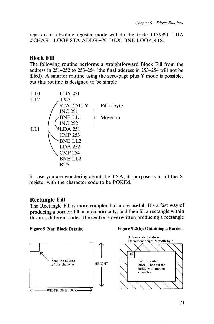
Chapter 9 Direct Routines

registers in absolute register mode will do the trick: LDX#0, LDA

#CHAR, :LOOP STA ADDR+X, DEX, BNE LOOP,RTS.

Block Fill

The following routine performs a straightforward Block Fill from the
address in 251-252 to 253-254 (the final address in 253-254 will not be
filled). A smarter routine using the zero-page plus Y mode is possible,
but this routine is designed to be simple.

:LL0
:LL2

:LL1

LDY #0
TXA
STA (251),Y
INC 251
BNE LL1
INC 252

‘LDA 251

CMP 253
BNE LL2
LDA 252
CMP 254
BNE LL2
RTS

Fill a byte

Move on

In case you are wondering about the TXA, its purpose is to fill the X
register with the character code to be POKEd.

Rectangle Fill

The Rectangle Fill is more complex but more useful. It’s a fast way of
producing a border: fill an area normally, and then fill a rectangle within
this in a different code. The centre is overwritten producing a rectangle

Figure 9.2(a): Block Details.

Figure 9.2(b): Obtaining a Border.

□

\

N Send the address

of this character

4

--------------

WIDTH OF BLOCK

------------

/K

HEIGHT

Nl/

Advance start address.
Decrement height & width by 2

71

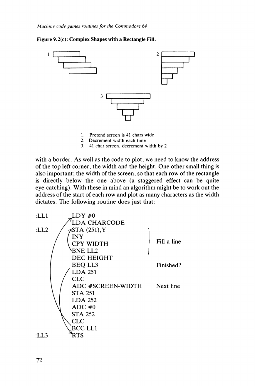
Machine code games routines for the Commodore 64

Figure 9.2(c): Complex Shapes with a Rectangle Fill.

3

U

1. Pretend screen is 41 chars wide

2. Decrement width each time

3. 41 char screen, decrement width by 2

with a border. As well as the code to plot, we need to know the address
of the top left corner, the width and the height. One other small thing is
also important; the width of the screen, so that each row of the rectangle
is directly below the one above (a staggered effect can be quite
eye-catching). With these in mind an algorithm might be to work out the
address of the start of each row and plot as many characters as the width
dictates. The following routine does just that:

:LL1
:LL2

:LL3

LD Y #0

LDA CHARCODE

71STA (251),Y

/ INY
l CPY WIDTH

'BNE LL2

DEC H EIGHT

BEQ LL3

LDA 251

CLC

ADC #SCREEN-WIDTH

STA 251

LDA 252

ADC #0

STA 252

CLC

BCC LL1

TS

Fill a line

Finished?

Next line

72

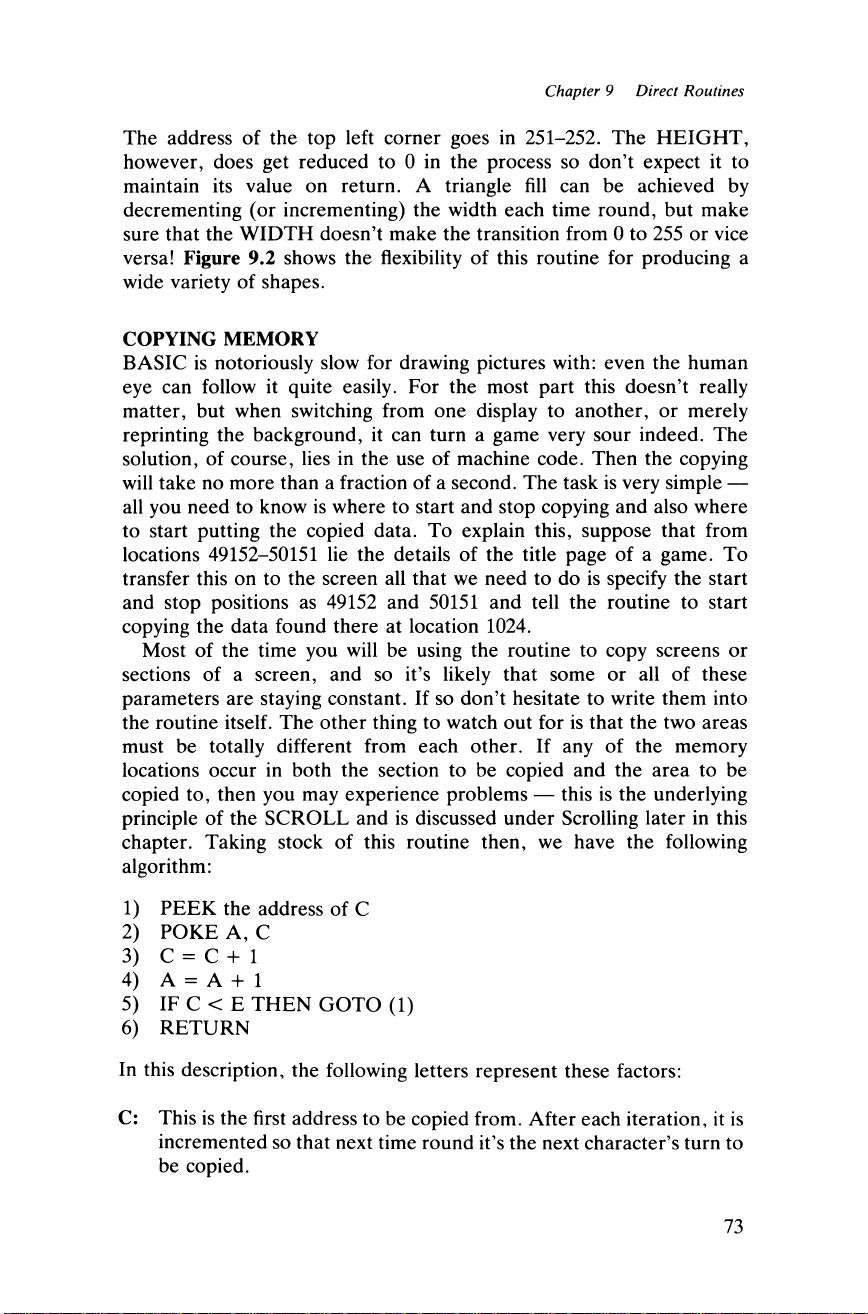
Chapter 9 Direct Routines

The address of the top left corner goes in 251-252. The HEIGHT,

however, does get reduced to 0 in the process so don’t expect it to
maintain its value on return. A triangle fill can be achieved by
decrementing (or incrementing) the width each time round, but make
sure that the WIDTH doesn’t make the transition from 0 to 255 or vice

versa! Figure 9.2 shows the flexibility of this routine for producing a
wide variety of shapes.

COPYING MEMORY
BASIC is notoriously slow for drawing pictures with: even the human
eye can follow it quite easily. For the most part this doesn’t really
matter, but when switching from one display to another, or merely
reprinting the background, it can turn a game very sour indeed. The
solution, of course, lies in the use of machine code. Then the copying
will take no more than a fraction of a second. The task is very simple —
all you need to know is where to start and stop copying and also where
to start putting the copied data. To explain this, suppose that from
locations 49152-50151 lie the details of the title page of a game. To
transfer this on to the screen all that we need to do is specify the start
and stop positions as 49152 and 50151 and tell the routine to start
copying the data found there at location 1024.

Most of the time you will be using the routine to copy screens or
sections of a screen, and so it’s likely that some or all of these
parameters are staying constant. If so don’t hesitate to write them into
the routine itself. The other thing to watch out for is that the two areas
must be totally different from each other. If any of the memory
locations occur in both the section to be copied and the area to be
copied to, then you may experience problems — this is the underlying
principle of the SCROLL and is discussed under Scrolling later in this
chapter. Taking stock of this routine then, we have the following
algorithm:

1) PEEK the address of C

2) POKE A, C

3) C = C + 1

4) A = A + 1

5) IF C < E THEN GOTO (1)

6) RETURN

In this description, the following letters represent these factors:

C: This is the first address to be copied from. After each iteration, it is

incremented so that next time round it’s the next character’s turn to
be copied.

73

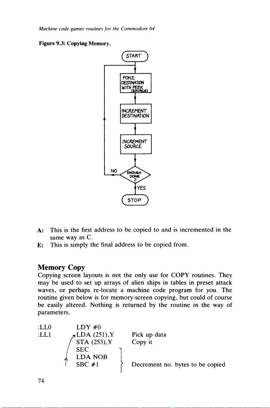
Machine code games routines for the Commodore 64

Figure 9.3: Copying Memory.

A: This is the first address to be copied to and is incremented in the

same way as C.

E: This is simply the final address to be copied from.

Memory Copy

Copying screen layouts is not the only use for COPY routines. They
may be used to set up arrays of alien ships in tables in preset attack

waves, or perhaps re-locate a machine code program for you. The

routine given below is for memory-screen copying, but could of course

be easily altered. Nothing is returned by the routine in the way of
parameters.

:LL0
:LL1

LDY #0
LDA (251),Y
STA (253),Y
SEC
LDA NOB
SBC #1

Pick up data
Copy it

Decrement no. bytes to be copied

74

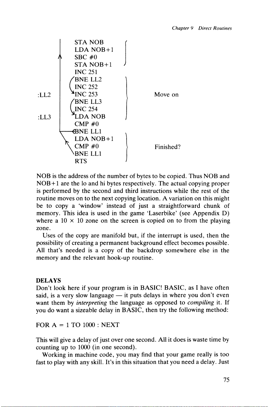
Chapter 9 Direct Routines

:LL2

:LL3

STA NOB
LDA NOB+1
SBC #0
STA NOB+1
INC 251

/B NE LL2

( INC 252

INC 253

/B NE LL3

INC 254
LDA NOB
CMP #0

<BNE LL1

LDA NOB + 1
CMP #0
BNE LL1
RTS

Move on

Finished?

NOB is the address of the number of bytes to be copied. Thus NOB and
NOB + 1 are the lo and hi bytes respectively. The actual copying proper
is performed by the second and third instructions while the rest of the
routine moves on to the next copying location. A variation on this might
be to copy a ‘window’ instead of just a straightforward chunk of
memory. This idea is used in the game ‘Laserbike’ (see Appendix D)
where a 10 x 10 zone on the screen is copied on to from the playing
zone.

Uses of the copy are manifold but, if the interrupt is used, then the
possibility of creating a permanent background effect becomes possible.
All that’s needed is a copy of the backdrop somewhere else in the
memory and the relevant hook-up routine.

DELAYS
Don’t look here if your program is in BASIC! BASIC, as I have often
said, is a very slow language — it puts delays in where you don’t even
want them by interpreting the language as opposed to compiling it. If
you do want a sizeable delay in BASIC, then try the following method:

FOR A = 1 TO 1000 : NEXT

This will give a delay of just over one second. All it does is waste time by
counting up to 1000 (in one second).

Working in machine code, you may find that your game really is too

fast to play with any skill. It’s in this situation that you need a delay. Just

75

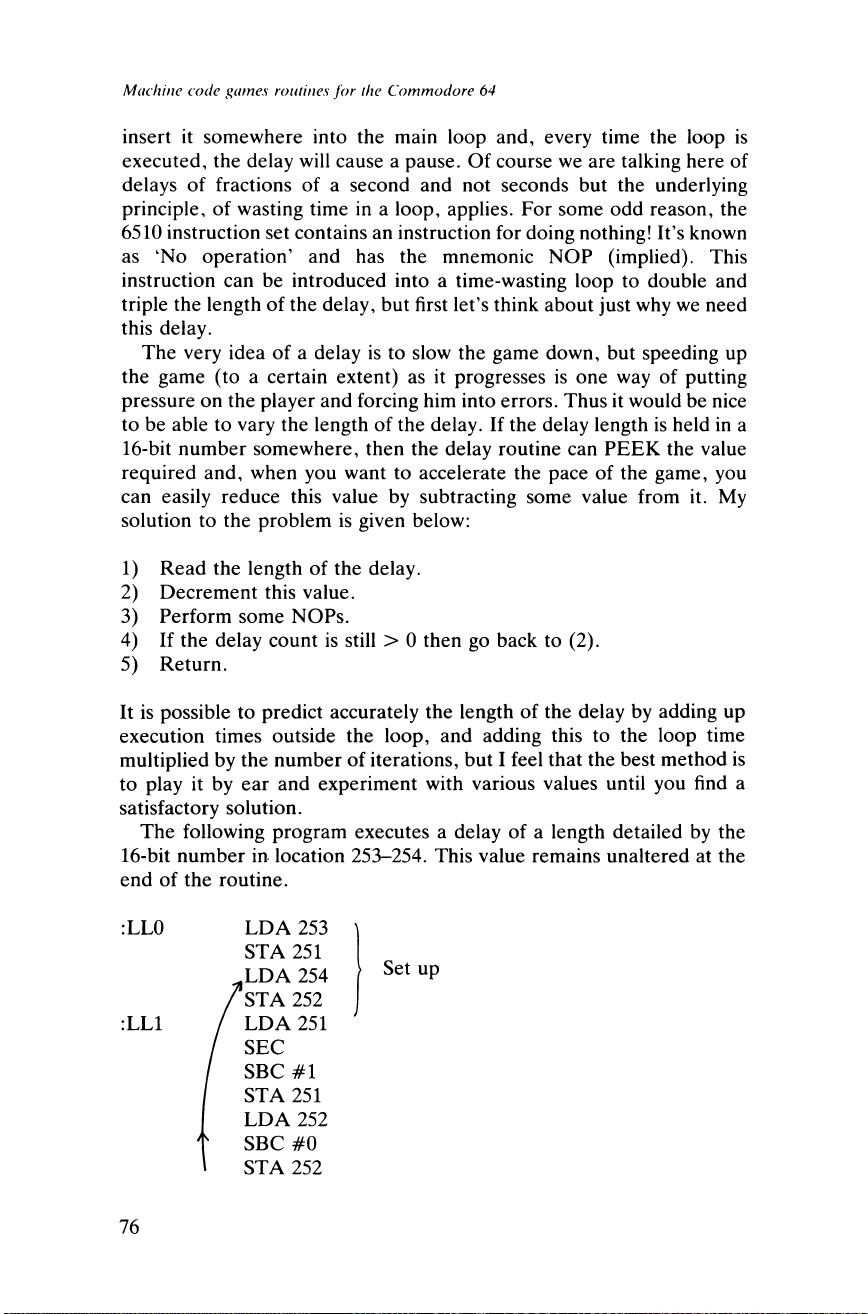
Machine code games routines for the Commodore 64

insert it somewhere into the main loop and, every time the loop is
executed, the delay will cause a pause. Of course we are talking here of
delays of fractions of a second and not seconds but the underlying
principle, of wasting time in a loop, applies. For some odd reason, the

6510 instruction set contains an instruction for doing nothing! It’s known

as ‘No operation’ and has the mnemonic NOP (implied). This

instruction can be introduced into a time-wasting loop to double and
triple the length of the delay, but first let’s think about just why we need
this delay.

The very idea of a delay is to slow the game down, but speeding up
the game (to a certain extent) as it progresses is one way of putting
pressure on the player and forcing him into errors. Thus it would be nice
to be able to vary the length of the delay. If the delay length is held in a

16-bit number somewhere, then the delay routine can PEEK the value
required and, when you want to accelerate the pace of the game, you
can easily reduce this value by subtracting some value from it. My
solution to the problem is given below:

1) Read the length of the delay.

2) Decrement this value.

3) Perform some NOPs.

4) If the delay count is still > 0 then go back to (2).

5) Return.

It is possible to predict accurately the length of the delay by adding up
execution times outside the loop, and adding this to the loop time
multiplied by the number of iterations, but I feel that the best method is
to play it by ear and experiment with various values until you find a
satisfactory solution.

The following program executes a delay of a length detailed by the
16-bit number in location 253-254. This value remains unaltered at the
end of the routine.

:LL0 LDA 253

ST A 251

Set up

:LL1

SBC #1
ST A 251
LDA 252

A SBC #0

> STA 252

76

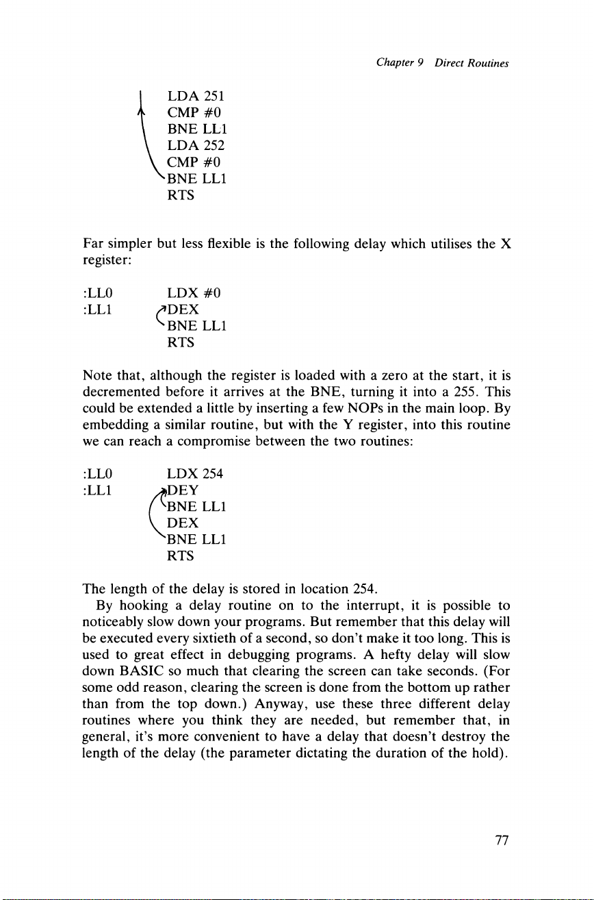
Chapter 9 Direct Routines

I LDA 251

\ CMP #0

\ BNE LL1

\ LDA 252

\ CMP #0

^BNE LL1

RTS

Far simpler but less flexible is the following delay which utilises the X
register:

:LL0 LDX #0
:LL1 /»DEX

^BNE LL1

RTS

Note that, although the register is loaded with a zero at the start, it is
decremented before it arrives at the BNE, turning it into a 255. This
could be extended a little by inserting a few NOPs in the main loop. By
embedding a similar routine, but with the Y register, into this routine
we can reach a compromise between the two routines:

:LL0 LDX 254
:LL1 >*DEY

A bNE LL1
V DEX

X BNE LL1

RTS

The length of the delay is stored in location 254.

By hooking a delay routine on to the interrupt, it is possible to
noticeably slow down your programs. But remember that this delay will
be executed every sixtieth of a second, so don’t make it too long. This is
used to great effect in debugging programs. A hefty delay will slow
down BASIC so much that clearing the screen can take seconds. (For
some odd reason, clearing the screen is done from the bottom up rather
than from the top down.) Anyway, use these three different delay
routines where you think they are needed, but remember that, in

general, it’s more convenient to have a delay that doesn’t destroy the

length of the delay (the parameter dictating the duration of the hold).

77

Machine code games routines for the Commodore 64

UPDATING BOMBS
If you have ever written a version of Space Invaders or the like in
BASIC, the chances are that the program was reasonably fast until the
bombing routine was put in. The bombs always spoil the action in any
BASIC arcade game as they take so long to update and check. Due to
this, some people write games without bombs and instead limit the
player to the number of shots he may use. This is a very poor substitute
and leads to a boring game.

The obvious answer is to include a machine code routine to handle the
bombing. All this does is search the screen for bombs, find them and
move them on to the next position, first checking to see if they have
crashed into something. If they have then this is flagged to the BASIC
(or machine code) program. Once this is done, all that remains is to call
the routine from BASIC with a single SYS call and check the contents of
the flag to see if a bomb has struck. There are two ways in which the
bombs can be moved. They can be kept on the screen and updated from
there, or they can be kept in a display file and manoeuvred from there.
It’s up to you to decide which system to use. The simplest way is
definitely the on-screen approach but this has the disadvantage that, if

the bombs are accidentally overwritten, they are lost. In the on-screen
system, all the BASIC program has to do is to POKE a bomb character

on to the screen at the right position. The machine code will then pick it
up and move it on from there. However, if you are scrolling the screen,
the bombs will acquire a sliding effect as well (this is not necessarily a
bad thing). The problem with the display file system is that, to eliminate
a bomb, you must go through the hassle of subtracting one element from
an array — a messy task. For details of the display file system, see the

section on moving groups of objects (Fleet Movements, in Chapter 10).

We will assume (for simplicity) that your bombs are going to fall
vertically (ie from top to bottom). Thus all the program has to do is to
scan the screen for the relevant PEEK code, blank out the bomb at its
present position and add 40, and plot it on again at the new position,
first checking to see if it’s going to hit something. If we think about it,

there are several things it could hit. It could hit part of the enemy (ie its
own side): this obviously doesn’t matter and the bomb will just have to
disappear. Or it could strike a protective hedge (like the ones in
Invaders). If this is the case, then the normal practice is to erode the
hedge and eliminate the bomb. The bomb could strike the bottom of the
screen and, when this happens, the bomb has clearly finished its useful

life. Thus we might as well destroy it. Some programmers like to have
their bombs explode when this happens — this is just an extra
refinement. The most important case is, of course, when the bomb
strikes the player’s ship. Differentiating between players’ ships and
other paraphernalia on the screen is largely up to the programmer. In

78

Chapter 9 Direct Routines

Space Invaders, one technique is to check only for a bomb-ship collision

when the bomb is near the bottom of the screen. The only thing the

bomb could hit on the line where the ship operates is the ship itself, and

so all the program has to do is check for a collision when the bomb

crosses this line. For more involved situations, the easiest method might

prove to be just looking at the PEEK codes and comparing them with

those of the ship and the other items.

This then gives the general idea of moving the bombs, but one or two
finer points arise out of it. Firstly you must scan the screen in the
opposite direction to that of bomb movement (this idea is met in
scrolling as well) as otherwise you will pick up a bomb and move it on,
only to pick it up again a fraction of an instant later (and move it on
again). Of course this results in the bombs moving straight to the base of
the screen in one scan. Secondly, don’t forget to reset the collision flag.
How this is done is important. You may want the bombs in the BASIC
program to move three times as fast as everything else. This can be
achieved by using:

SYS 826 : SYS 826 : SYS 826

(826 is the assumed address of the routine.) If this is the case, then it’s
no use the machine code routine resetting the flag: the flag might be lost

if a collision occurred in the first one or two passes. In this instance it’s
the caller that must maintain the status of the flag, but bear in mind this
is not always the case.

We are now in a position to set down the various stages involved in

the bomb-updating process:

1) Reset the collision flag (may be omitted).

2) Scan screen in opposite sense to bomb motion.

3) If bomb has hit something other than the player’s property, then

apply rules of the game to the situation.

4) If the bomb has hit the player’s ship, then set the collision flag.

5) Repeat (2) onwards until the screen has been scanned.

If the bomb does hit something then the programmer might want to
trigger an explosion by tripping a gate in the SID.

To alter the direction of the bombs all you have to do is to alter the

bomb vector, but bear in mind that if you make the bombs move into

progressively lower memory locations then you will have to reverse the

direction of the scan. To liven things up a bit you might like to try a
‘spiralling’ bomb routine where the bombs change shape as they fall.
The best way to do this is to alter the UDG definition from one shape to
another, every time the routine is called. Using this method I have

79

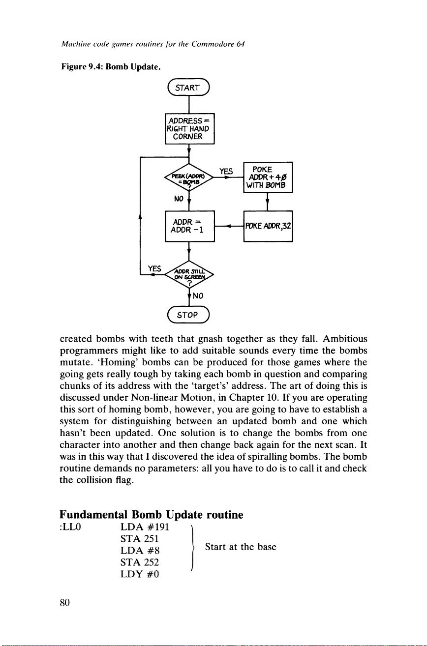
Machine code games routines for the Commodore 64

Figure 9.4: Bomb Update.

created bombs with teeth that gnash together as they fall. Ambitious
programmers might like to add suitable sounds every time the bombs
mutate. ‘Homing’ bombs can be produced for those games where the
going gets really tough by taking each bomb in question and comparing
chunks of its address with the ‘target’s’ address. The art of doing this is
discussed under Non-linear Motion, in Chapter 10. If you are operating
this sort of homing bomb, however, you are going to have to establish a

system for distinguishing between an updated bomb and one which

hasn’t been updated. One solution is to change the bombs from one
character into another and then change back again for the next scan. It
was in this way that I discovered the idea of spiralling bombs. The bomb
routine demands no parameters: all you have to do is to call it and check
the collision flag.

Fundamental Bomb Update routine

:LL0 LDA #191

ST A 251
LDA #8
STA 252
LDY #0

Start at the base

80

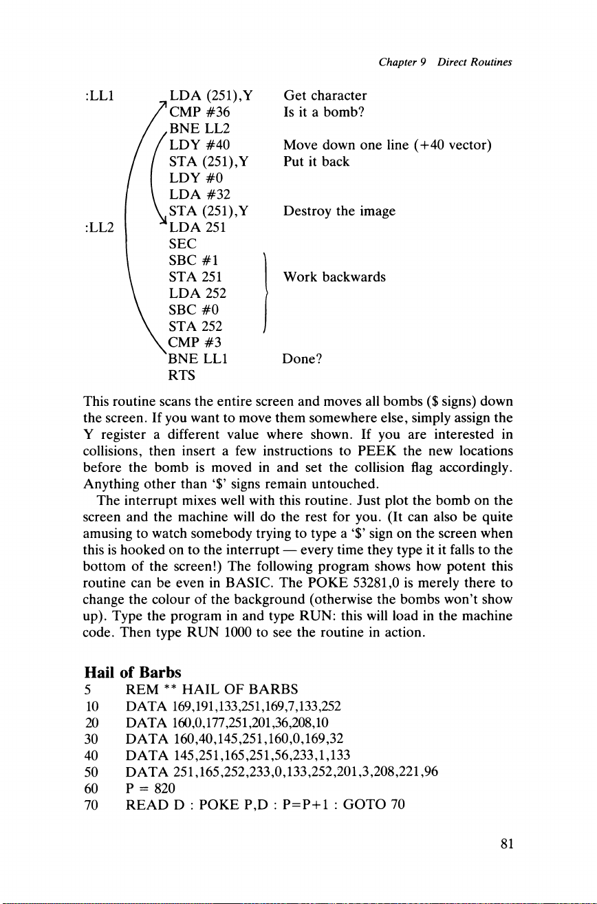
Chapter 9 Direct Routines

:LL1 LDA (251),Y

Get character

Is it a bomb?CMP #36
BNE LL2
LDY #40 Move down one line (+40 vector)

Put it backSTA (251),Y
LDY #0
LDA #32
STA (251),Y Destroy the image

:LL2 LDA 251

SEC
SBC #1
STA 251
LDA 252
SBC #0
STA 252

CMP #3
BNE LL1
RTS

Done?

Work backwards

This routine scans the entire screen and moves all bombs ($ signs) down
the screen. If you want to move them somewhere else, simply assign the
Y register a different value where shown. If you are interested in
collisions, then insert a few instructions to PEEK the new locations
before the bomb is moved in and set the collision flag accordingly.
Anything other than *$’ signs remain untouched.

The interrupt mixes well with this routine. Just plot the bomb on the
screen and the machine will do the rest for you. (It can also be quite
amusing to watch somebody trying to type a *$’ sign on the screen when
this is hooked on to the interrupt — every time they type it it falls to the
bottom of the screen!) The following program shows how potent this
routine can be even in BASIC. The POKE 53281,0 is merely there to
change the colour of the background (otherwise the bombs won’t show
up). Type the program in and type RUN: this will load in the machine
code. Then type RUN 1000 to see the routine in action.

Hail of Barbs

5 REM ** HAIL OF BARBS

10 DATA 169,191,133,251,169,7,133,252

20 DATA 160,0,177,251,201,36,208,10
30 DATA 160,40,145,251,160,0,169,32
40 DATA 145,251,165,251,56,233,1,133
50 DATA 251,165,252,233,0,133,252,201,3,208,221,96

60 P = 820
70 READ D : POKE P,D : P=P+1 : GOTO 70

81

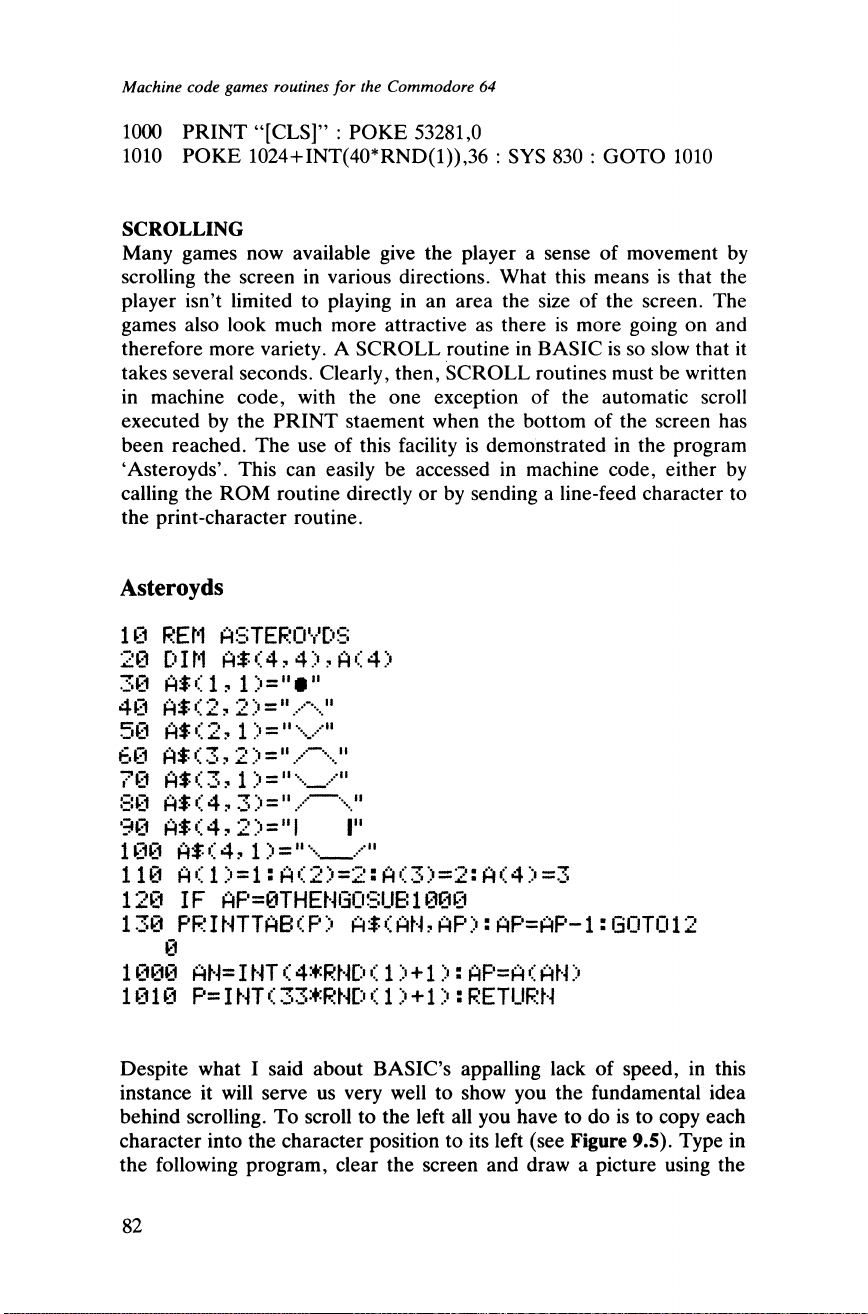
Machine code games routines for the Commodore 64

1000 PRINT “[CLS]” : POKE 53281,0

1010 POKE 1024+INT(40*RND(1)),36 : SYS 830 : GOTO 1010

SCROLLING

Many games now available give the player a sense of movement by
scrolling the screen in various directions. What this means is that the

player isn’t limited to playing in an area the size of the screen. The

games also look much more attractive as there is more going on and
therefore more variety. A SCROLL routine in BASIC is so slow that it
takes several seconds. Clearly, then, SCROLL routines must be written
in machine code, with the one exception of the automatic scroll

executed by the PRINT staement when the bottom of the screen has

been reached. The use of this facility is demonstrated in the program
‘Asteroyds’. This can easily be accessed in machine code, either by

calling the ROM routine directly or by sending a line-feed character to
the print-character routine.

Asteroyds

10 REM ASTERQVDS
20 DIM AS < 4.- 4 > > A < 4 >
30 ASCI, l>=,,*n

40 AS<2, 2> = ",-"\"

50 AS <2,1 > =

60 AS<3,2>="/“\ H

70 AS < 3 ? 1 > = "
80 AS<4,3>=".-••—
90 AS<4? 2>="l I"

100 AS (4,1 ) = "\

__

110 A<1} = 1:A(2>=2:A(3)=2:A<4> =3
120 IF AP=0THENSOSUB1000
130 PRINTTAB< P > AS <AN,AP>:AP=AP-1:GOTO12

0

1@00 AN=INT < 4*RND<1> +1):AP=A <AN >
1010 P= I NT 33*RND < 1 > +1 > : RETURN

Despite what I said about BASIC’s appalling lack of speed, in this
instance it will serve us very well to show you the fundamental idea
behind scrolling. To scroll to the left all you have to do is to copy each
character into the character position to its left (see Figure 9.5). Type in
the following program, clear the screen and draw a picture using the

8 2

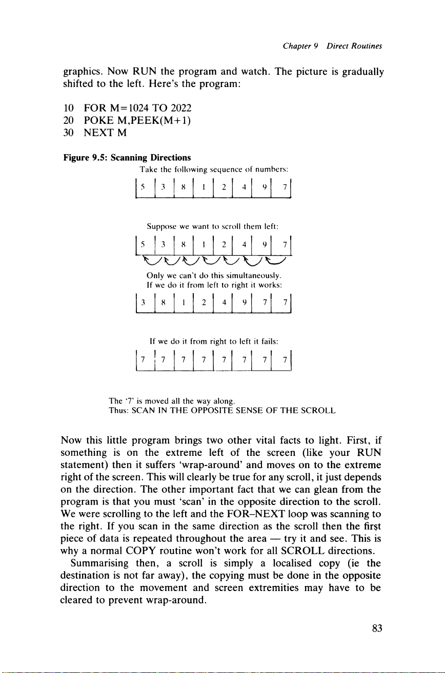
Chapter 9 Direct Routines

graphics. Now RUN the program and watch. The picture is gradually
shifted to the left. Here’s the program:

10 FOR M=1024 TO 2022
20 POKE M,PEEK(M+1)
30 NEXT M

Figure 9.5: Scanning Directions

Take the following sequence of numbers:

5 3 8 1 2 4 9 7

Suppose we want to scroll them left:

Only we can’t do this simultaneously.
If we do it from left to right it works:

3 8 1 2 4 9 7 7

If we do it from right to left it fails:

7 ! 7 7 7 7 7 7 7

The ‘7’ is moved all the way along.
Thus: SCAN IN THE OPPOSITE SENSE OF THE SCROLL

Now this little program brings two other vital facts to light. First, if
something is on the extreme left of the screen (like your RUN
statement) then it suffers ‘wrap-around’ and moves on to the extreme
right of the screen. This will clearly be true for any scroll, it just depends
on the direction. The other important fact that we can glean from the
program is that you must ‘scan’ in the opposite direction to the scroll.
We were scrolling to the left and the FOR-NEXT loop was scanning to
the right. If you scan in the same direction as the scroll then the fir§t
piece of data is repeated throughout the area — try it and see. This is
why a normal COPY routine won’t work for all SCROLL directions.

Summarising then, a scroll is simply a localised copy (ie the
destination is not far away), the copying must be done in the opposite
direction to the movement and screen extremities may have to be
cleared to prevent wrap-around.

83

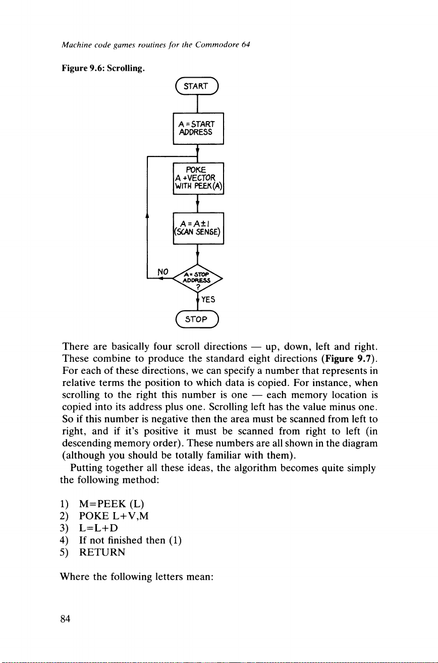
Machine code games routines for the Commodore 64

Figure 9.6: Scrolling.

There are basically four scroll directions — up, down, left and right.
These combine to produce the standard eight directions (Figure 9.7).
For each of these directions, we can specify a number that represents in
relative terms the position to which data is copied. For instance, when
scrolling to the right this number is one — each memory location is
copied into its address plus one. Scrolling left has the value minus one.
So if this number is negative then the area must be scanned from left to
right, and if it’s positive it must be scanned from right to left (in
descending memory order). These numbers are all shown in the diagram
(although you should be totally familiar with them).

Putting together all these ideas, the algorithm becomes quite simply

the following method:

1) M=PEEK (L)

2) POKE L+V,M

3) L=L+D

4) If not finished then (1)

5) RETURN

Where the following letters mean:

84

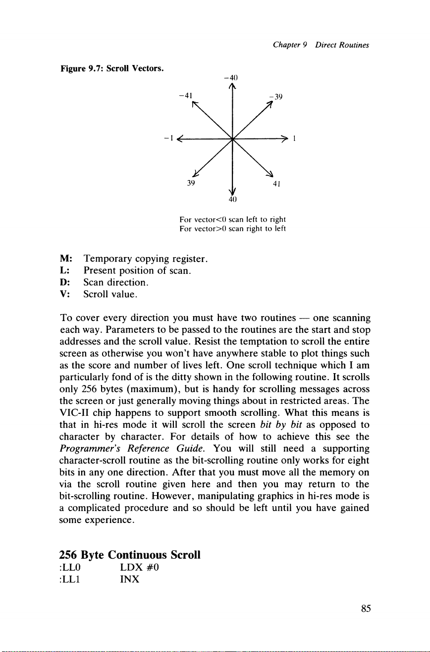
Chapter 9 Direct Routines

Figure 9.7: Scroll Vectors.

-4 0

For vector<0 scan left to right
For vector>() scan right to left

M: Temporary copying register.
L: Present position of scan.
D: Scan direction.
V: Scroll value.

To cover every direction you must have two routines — one scanning

each way. Parameters to be passed to the routines are the start and stop
addresses and the scroll value. Resist the temptation to scroll the entire
screen as otherwise you won’t have anywhere stable to plot things such
as the score and number of lives left. One scroll technique which I am
particularly fond of is the ditty shown in the following routine. It scrolls

only 256 bytes (maximum), but is handy for scrolling messages across
the screen or just generally moving things about in restricted areas. The
VIC-II chip happens to support smooth scrolling. What this means is
that in hi-res mode it will scroll the screen bit by bit as opposed to
character by character. For details of how to achieve this see the

Programmer s Reference Guide. You will still need a supporting

character-scroll routine as the bit-scrolling routine only works for eight
bits in any one direction. After that you must move all the memory on
via the scroll routine given here and then you may return to the
bit-scrolling routine. However, manipulating graphics in hi-res mode is
a complicated procedure and so should be left until you have gained
some experience.

256 Byte Continuous Scroll

:LL0 LDX #0
:LL1 INX

85

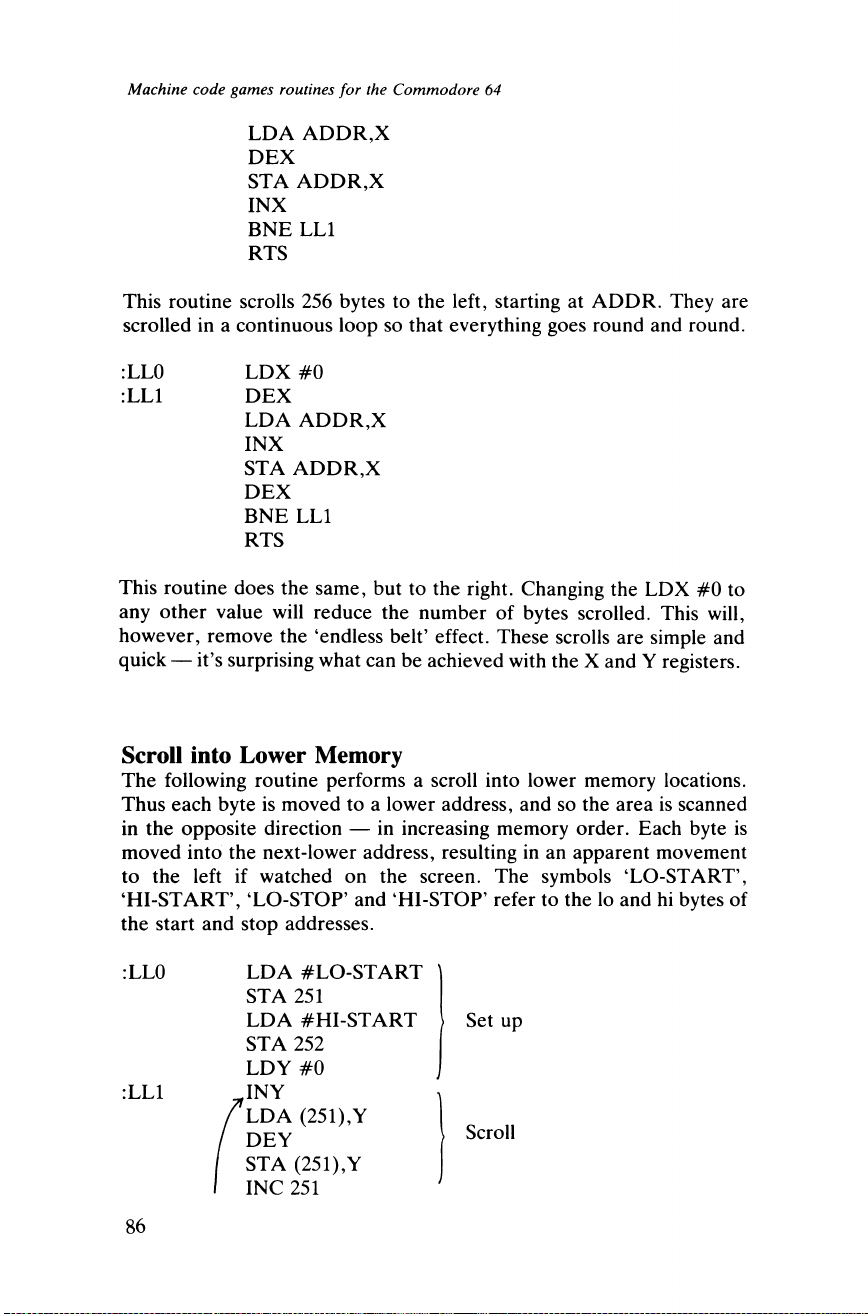
Machine code games routines for the Commodore 64

LDA ADDR,X
DEX
STA ADDR,X
INX
BNE LL1
RTS

This routine scrolls 256 bytes to the left, starting at ADDR. They are

scrolled in a continuous loop so that everything goes round and round.

:LL0
:LL1

LDX #0
DEX
LDA ADDR,X
INX
STA ADDR,X
DEX
BNE LL1
RTS

This routine does the same, but to the right. Changing the LDX #0 to
any other value will reduce the number of bytes scrolled. This will,
however, remove the ‘endless belt’ effect. These scrolls are simple and
quick — it’s surprising what can be achieved with the X and Y registers.

Scroll into Lower Memory

The following routine performs a scroll into lower memory locations.
Thus each byte is moved to a lower address, and so the area is scanned

in the opposite direction — in increasing memory order. Each byte is

moved into the next-lower address, resulting in an apparent movement

to the left if watched on the screen. The symbols ‘LO-START’,
‘HI-START’, ‘LO-STOP’ and ‘HI-STOP’ refer to the lo and hi bytes of
the start and stop addresses.

:LL0 LDA #LO-START

STA 251
LDA #HI-START Set up
STA 252
LDY #0
INY ,

(251),Y „

:LL1

Scroll

STA (251),Y
INC 251

8 6

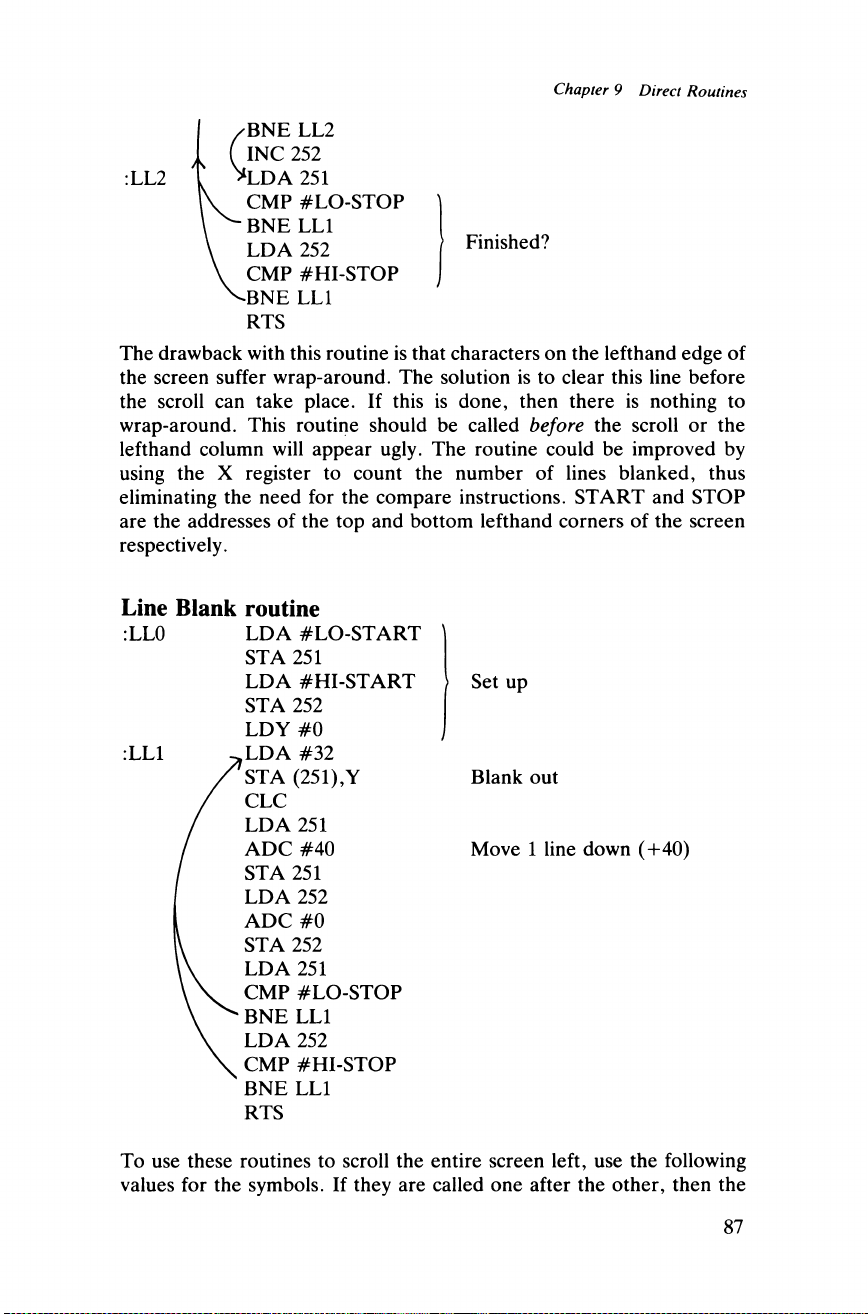
Chapter 9 Direct Routines

:LL2

c

BNE LL2
INC 252
LDA 251
CMP #LO-STOP
BNE LL1
LDA 252
CMP #HI-STOP
BNE LL1
RTS

Finished?

The drawback with this routine is that characters on the lefthand edge of
the screen suffer wrap-around. The solution is to clear this line before
the scroll can take place. If this is done, then there is nothing to
wrap-around. This routine should be called before the scroll or the
lefthand column will appear ugly. The routine could be improved by
using the X register to count the number of lines blanked, thus
eliminating the need for the compare instructions. START and STOP
are the addresses of the top and bottom lefthand corners of the screen
respectively.

Line Blank routine

:LL0

:LL1

LDA #LO-START
STA 251
LDA #HI-START
STA 252
LDY #0
LDA #32
STA (251),Y
CLC
LDA 251
ADC #40
STA 251
LDA 252
ADC #0
STA 252
LDA 251
CMP #LO-STOP
BNE LL1
LDA 252
CMP #HI-STOP

BNE LL1

RTS

Set up

Blank out

Move 1 line down (+40)

To use these routines to scroll the entire screen left, use the following
values for the symbols. If they are called one after the other, then the

87

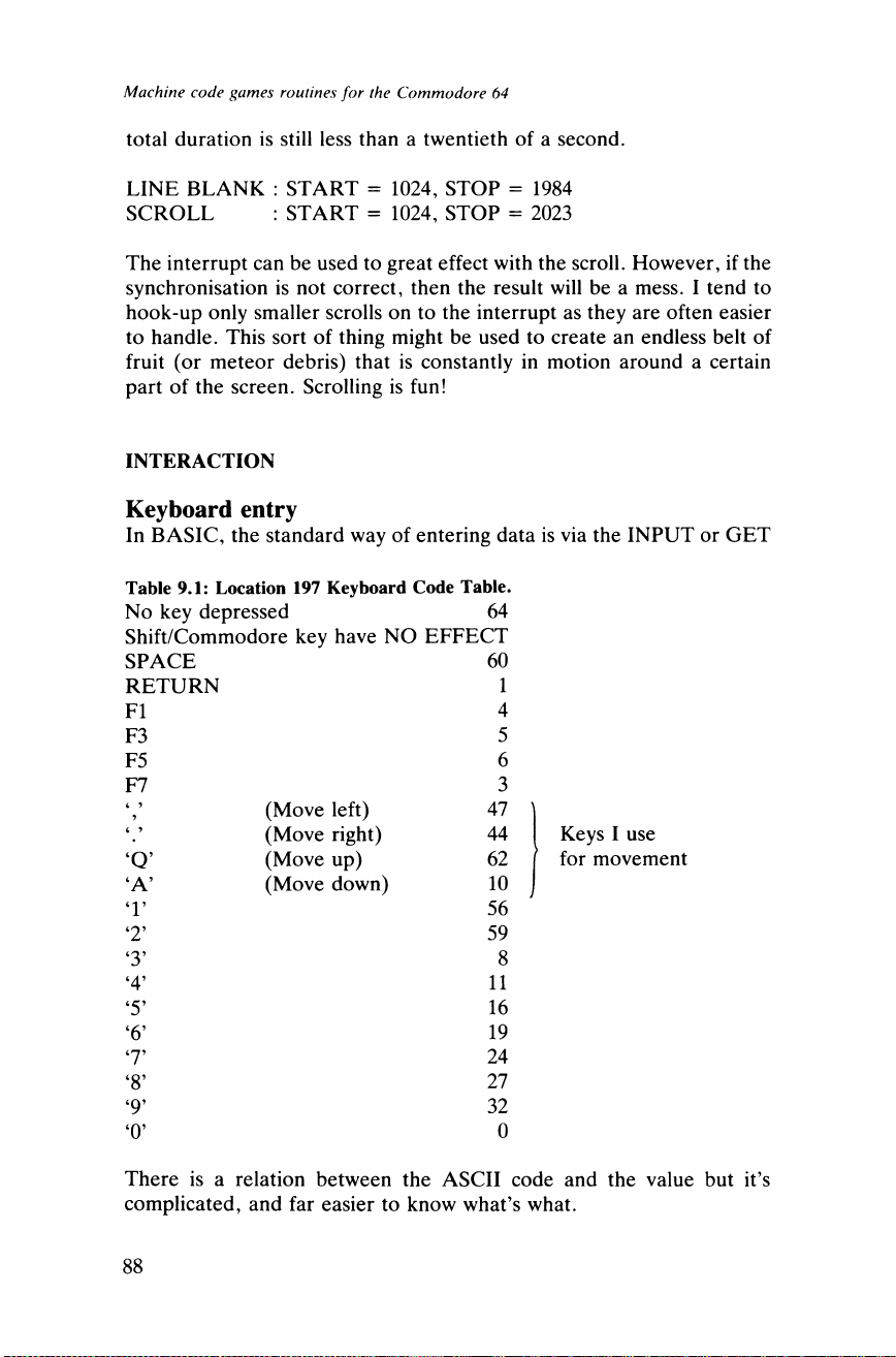
Machine code games routines for the Commodore 64

total duration is still less than a twentieth of a second.

LINE BLANK : START = 1024, STOP = 1984
SCROLL : START = 1024, STOP = 2023

The interrupt can be used to great effect with the scroll. However, if the
synchronisation is not correct, then the result will be a mess. I tend to
hook-up only smaller scrolls on to the interrupt as they are often easier
to handle. This sort of thing might be used to create an endless belt of
fruit (or meteor debris) that is constantly in motion around a certain
part of the screen. Scrolling is fun!

INTERACTION

Keyboard entry

In BASIC, the standard way of entering data is via the INPUT or GET

Table 9.1: Location 197 Keyboard Code Table.

No key depressed 64
Shift/Commodore key have NO EFFECT
SPACE
RETURN
FI
F3
F5
F7

60

1
4
5
6
3

t 7

7

(Move left)

47

t 7

(Move right)

44

‘Q’

(Move up)

62

‘A’

(Move down)

10

T

56

‘2’

59

‘3’

8

‘4’

11

‘5’

16

‘6’

19

‘7’

24

‘8’

27

‘9’

32

‘0’

0

Keys I use
for movement

There is a relation between the ASCII code and the value but it’s
complicated, and far easier to know what’s what.

88

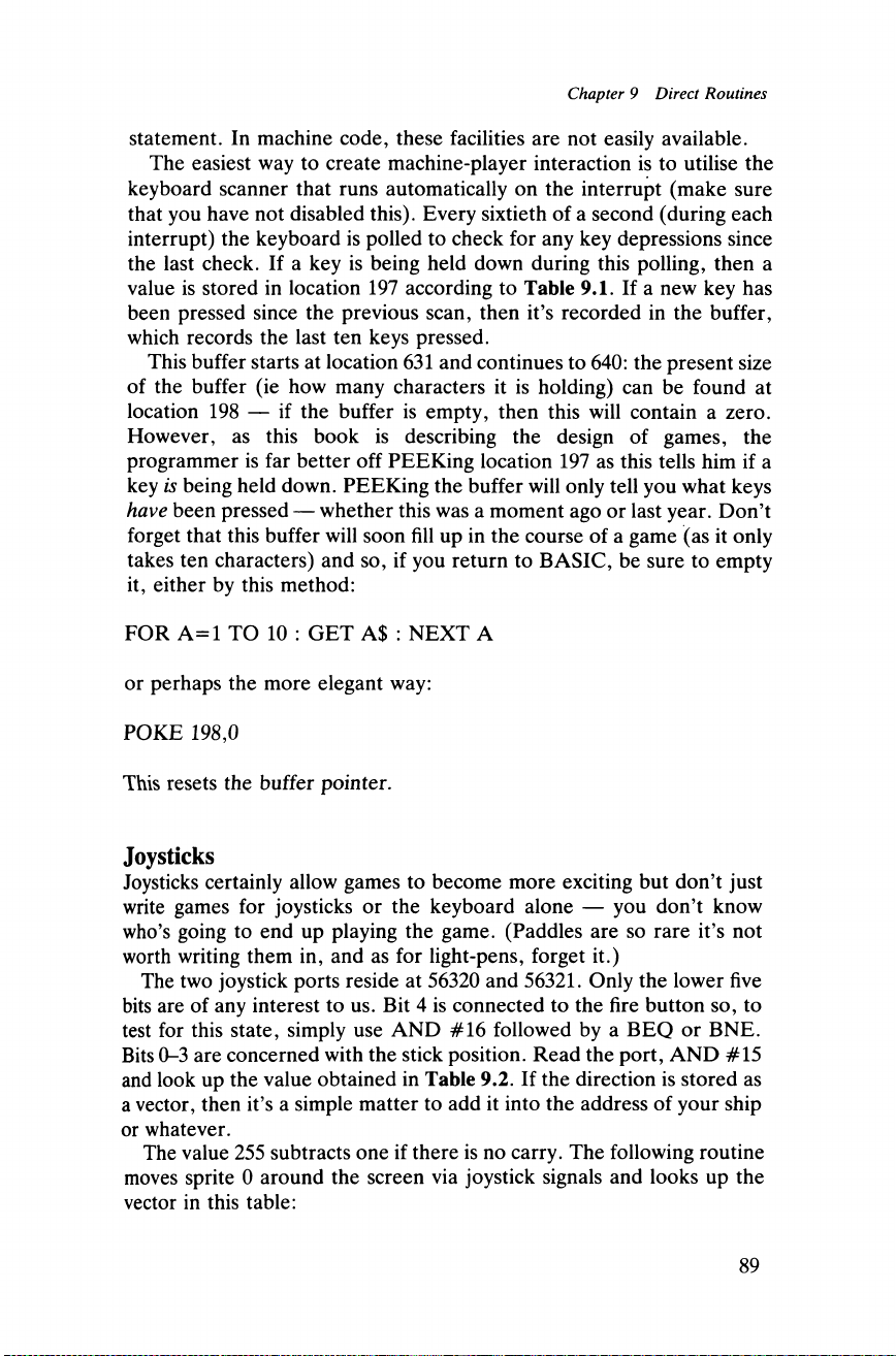
Chapter 9 Direct Routines

statement. In machine code, these facilities are not easily available.

The easiest way to create machine-player interaction is to utilise the
keyboard scanner that runs automatically on the interrupt (make sure
that you have not disabled this). Every sixtieth of a second (during each
interrupt) the keyboard is polled to check for any key depressions since
the last check. If a key is being held down during this polling, then a
value is stored in location 197 according to Table 9.1. If a new key has
been pressed since the previous scan, then it’s recorded in the buffer,

which records the last ten keys pressed.

This buffer starts at location 631 and continues to 640: the present size

of the buffer (ie how many characters it is holding) can be found at

location 198 — if the buffer is empty, then this will contain a zero.

However, as this book is describing the design of games, the
programmer is far better off PEEKing location 197 as this tells him if a
key is being held down. PEEKing the buffer will only tell you what keys
have been pressed — whether this was a moment ago or last year. Don’t

forget that this buffer will soon fill up in the course of a game (as it only

takes ten characters) and so, if you return to BASIC, be sure to empty

it, either by this method:

FOR A=1 TO 10 : GET A$ : NEXT A

or perhaps the more elegant way:

POKE 198,0

This resets the buffer pointer.

Joysticks

Joysticks certainly allow games to become more exciting but don’t just
write games for joysticks or the keyboard alone — you don’t know
who’s going to end up playing the game. (Paddles are so rare it’s not

worth writing them in, and as for light-pens, forget it.)

The two joystick ports reside at 56320 and 56321. Only the lower five
bits are of any interest to us. Bit 4 is connected to the fire button so, to
test for this state, simply use AND #16 followed by a BEQ or BNE.
Bits 0-3 are concerned with the stick position. Read the port, AND #15
and look up the value obtained in Table 9.2. If the direction is stored as
a vector, then it’s a simple matter to add it into the address of your ship
or whatever.

The value 255 subtracts one if there is no carry. The following routine

moves sprite 0 around the screen via joystick signals and looks up the

vector in this table:

89

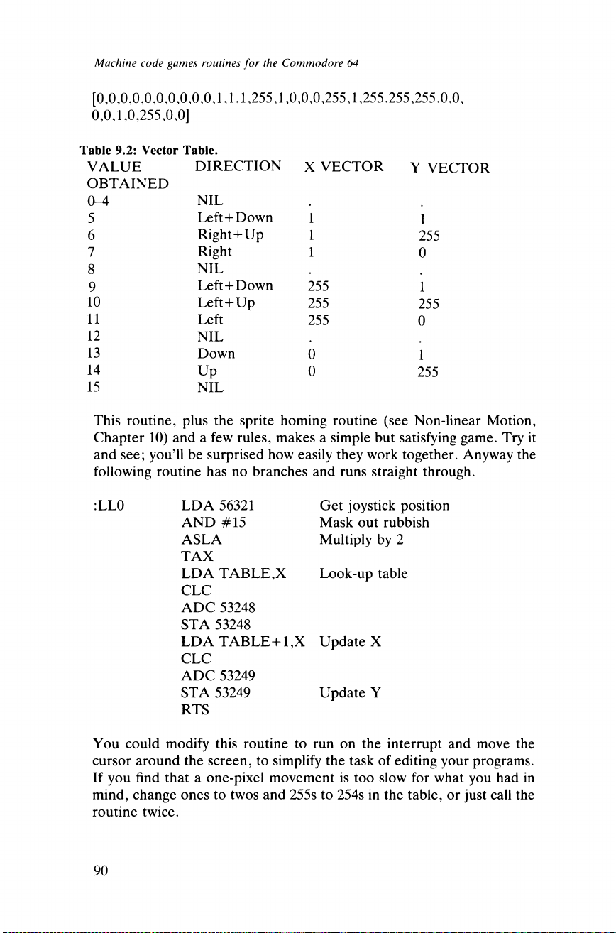
Machine code games routines for the Commodore 64

[0,0,0,0,0,0,0,0,0,0,1,1,1,255,1,0,0,0,255,1,255,255,255,0,0,
0,0,1,0,255,0,0]

Table 9.2: Vector Table.

VALUE

OBTAINED

DIRECTION

X VECTOR

Y VECTOR

0-4

NIL

5

Left+ Down

1

1

6

Right+Up

1

255

7

Right

1

0

8

NIL

9

Left 4- Down

255

1

10

Left 4- Up

255

255

11

Left

255

0

12

NIL

13

Down

0

1

14
15

Up
NIL

0

255

This routine, plus the sprite homing routine (see Non-linear Motion,
Chapter 10) and a few rules, makes a simple but satisfying game. Try it
and see; you’ll be surprised how easily they work together. Anyway the
following routine has no branches and runs straight through.

:LL0 LDA 56321

AND #15
ASLA
TAX
LDA TABLE,X
CLC
ADC 53248
STA 53248
LDA TABLET 1,X
CLC
ADC 53249
STA 53249
RTS

Get joystick position
Mask out rubbish
Multiply by 2

Look-up table

Update X

Update Y

You could modify this routine to run on the interrupt and move the
cursor around the screen, to simplify the task of editing your programs.
If you find that a one-pixel movement is too slow for what you had in
mind, change ones to twos and 255s to 254s in the table, or just call the
routine twice.

90