ST AN2615 Application note

AN2615

Application note

A high precision, low cost, single supply ADC for positive and negative input voltages

Introduction

In general the ADC embedded in the ST7 microcontroller is enough for most applications. But, in some cases it is necessary to measure both positive and negative voltages. This requires an external ADC with this particular capability. Most external ADCs require a dual supply to be able to do this. However, microcontroller-based applications usually only have a positive supply available.

This application note describes a technique for implementing an ADC for measuring both positive and negative input voltages while operating from a single (positive) supply. This converter is based on a voltage-to-time conversion technique. Like other slope converters, this ADC also uses an integrating capacitor, but the measured time is inversely proportional to the input voltage. An additional comparator with a voltage reference is used to improve conversion accuracy.

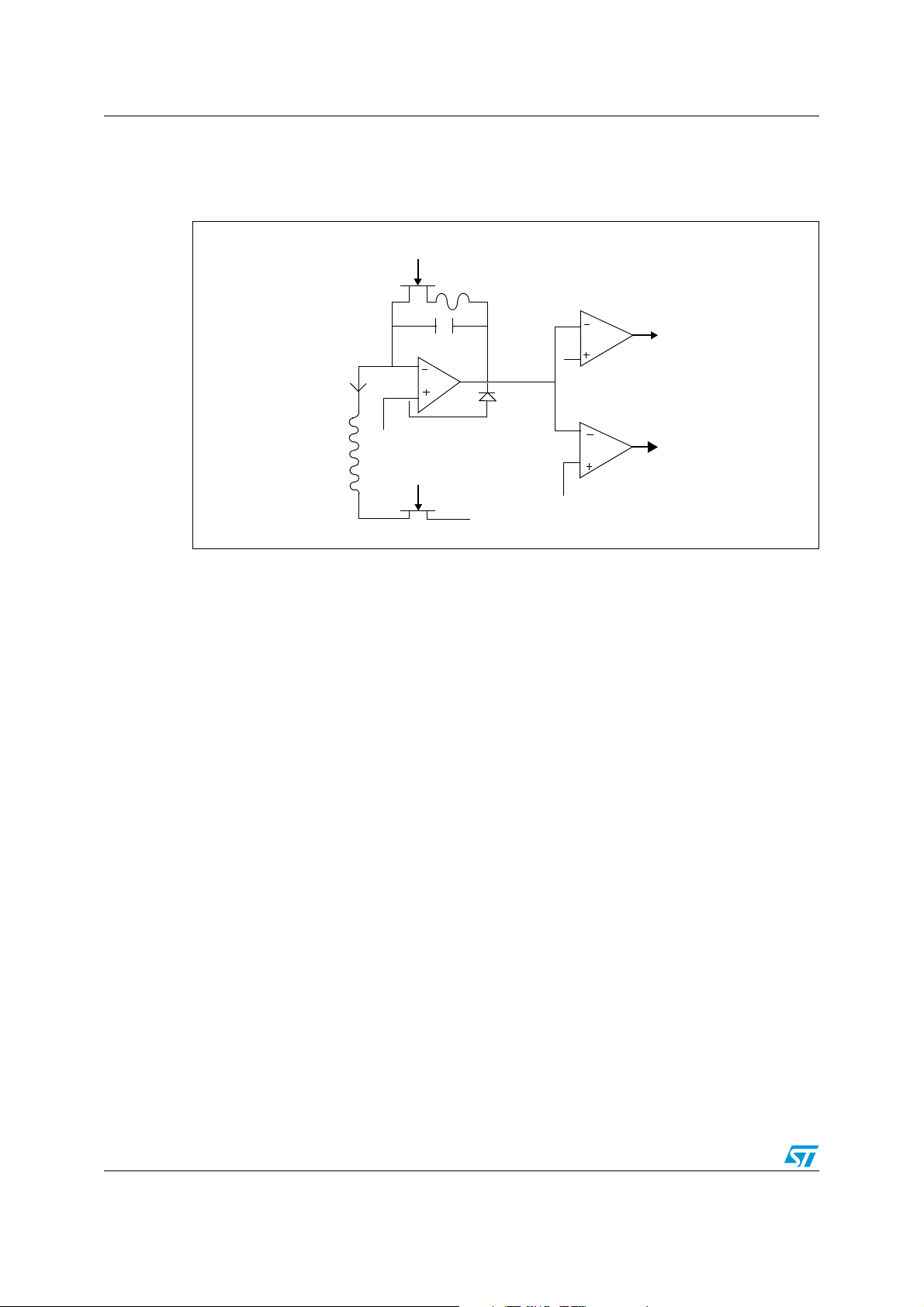
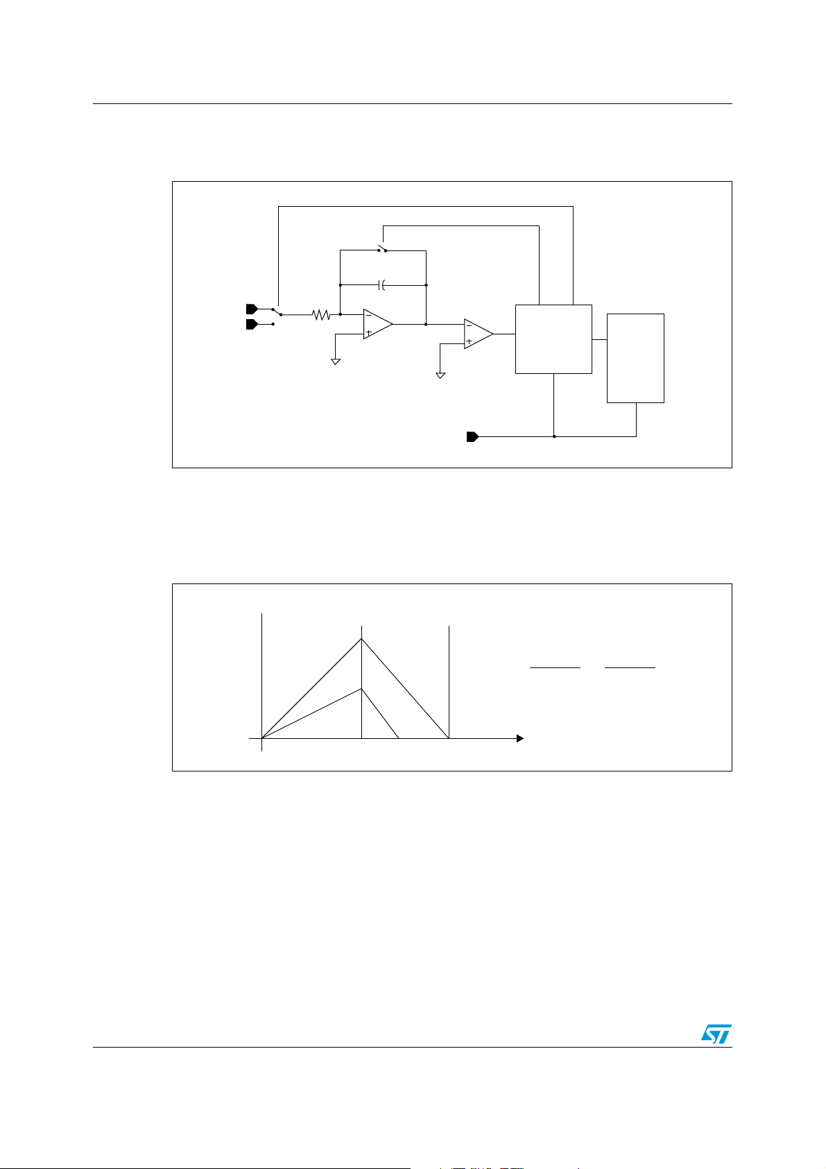
As shown in the circuit diagram (Figure 1 on page 6), the converter is implemented using an integrating capacitor, resistor, external op-amp, comparators and some microcontroller I/O pins. The ST72F264 microcontroller is used in this application note as an example, but the implementation is feasible using any ST7 microcontroller. The 16-bit timer of the microcontroller measures the time using its input capture pins (PB0 and PB2). These pins are connected to the output of the Comp1 and Comp2 comparators. The I/O pins PB1 and PB3 are used to switch the M1 and M2 switches on or off. The circuit could also work with a microcontroller equipped with an 8-bit timer. Only a small modification to the software would be needed.

August 2007

Rev 1

1/37

www.st.com

Contents	AN2615

Contents

1	Circuit diagram . . . . . . . . . . . . . . . . . . . . . . . . . . . . . . . . . . . . . . . . . . . .			. 6
2	Theory of operation . . . . . . . . . . . . . . . . . . . . . . . . . . . . . . . . . . . . . . . . .			7
	2.1	Advantage of using two comparators . . . . . . . . . . . . . . . . . . . . . . . . . . . . .		7
3	Timing diagram . . . . . . . . . . . . . . . . . . . . . . . . . . . . . . . . . . . . . . . . . . . . .			8
4	Circuit analysis . . . . . . . . . . . . . . . . . . . . . . . . . . . . . . . . . . . . . . . . . . . . .			9
5	Vout vs time diagram for different input voltages . . . . . . . . . . . . . . . . .			10
6	Characteristics of different slope converters . . . . . . . . . . . . . . . . . . . .			11
	6.1	Single-slope converter . . . . . . . . . . . . . . . . . . . . . . . . . . . . . . . . . . . . . . .		11
		6.1.1	Single-slope converter timing diagram . . . . . . . . . . . . . . . . . . . . . . . . . .	11
	6.2	Dual-slope converter . . . . . . . . . . . . . . . . . . . . . . . . . . . . . . . . . . . . . . . .		12
		6.2.1	Dual-slope converter timing diagram . . . . . . . . . . . . . . . . . . . . . . . . . . .	12
	6.3	Solution presented in this application note . . . . . . . . . . . . . . . . . . . . . . . .		13
7	Error analysis/constraints . . . . . . . . . . . . . . . . . . . . . . . . . . . . . . . . . . .			14

7.1 Input offset voltage . . . . . . . . . . . . . . . . . . . . . . . . . . . . . . . . . . . . . . . . . . 14 7.2 Correction factor for the product of R*C . . . . . . . . . . . . . . . . . . . . . . . . . . 14 7.3 Value of charging resistance R . . . . . . . . . . . . . . . . . . . . . . . . . . . . . . . . . 14 7.4 Charging capacitor C . . . . . . . . . . . . . . . . . . . . . . . . . . . . . . . . . . . . . . . . 14 7.5 16-bit timer . . . . . . . . . . . . . . . . . . . . . . . . . . . . . . . . . . . . . . . . . . . . . . . . 15 7.6 Effect of temperature . . . . . . . . . . . . . . . . . . . . . . . . . . . . . . . . . . . . . . . . 15 7.7 Comparator . . . . . . . . . . . . . . . . . . . . . . . . . . . . . . . . . . . . . . . . . . . . . . . 15

8	Voltage references . . . . . . . . . . . . . . . . . . . . . . . . . . . . . . . . . . . . . . . . .	16
9	Hardware setup . . . . . . . . . . . . . . . . . . . . . . . . . . . . . . . . . . . . . . . . . . . .	17
10	Algorithm . . . . . . . . . . . . . . . . . . . . . . . . . . . . . . . . . . . . . . . . . . . . . . . . .	18
11	Result . . . . . . . . . . . . . . . . . . . . . . . . . . . . . . . . . . . . . . . . . . . . . . . . . . . .	19
2/37

AN2615	Contents

11.1 Positive input . . . . . . . . . . . . . . . . . . . . . . . . . . . . . . . . . . . . . . . . . . . . . . 19 11.2 Negative input . . . . . . . . . . . . . . . . . . . . . . . . . . . . . . . . . . . . . . . . . . . . . 23 11.3 Effect of the capacitor value . . . . . . . . . . . . . . . . . . . . . . . . . . . . . . . . . . . 26

12 Conclusion . . . . . . . . . . . . . . . . . . . . . . . . . . . . . . . . . . . . . . . . . . . . . . . . 27

13 References and bibliography . . . . . . . . . . . . . . . . . . . . . . . . . . . . . . . . . 28

Appendix A Input stage conditions. . . . . . . . . . . . . . . . . . . . . . . . . . . . . . . . . . . . 29

A.1 Case 1: Voltage measurement . . . . . . . . . . . . . . . . . . . . . . . . . . . . . . . . . 29 A.2 Case 2: Current measurement . . . . . . . . . . . . . . . . . . . . . . . . . . . . . . . . . 30

Appendix B Application board schematics . . . . . . . . . . . . . . . . . . . . . . . . . . . . . 31

Appendix C Bill of materials . . . . . . . . . . . . . . . . . . . . . . . . . . . . . . . . . . . . . . . . . 32

Appendix D Software flow . . . . . . . . . . . . . . . . . . . . . . . . . . . . . . . . . . . . . . . . . . . 34

D.1 Code size . . . . . . . . . . . . . . . . . . . . . . . . . . . . . . . . . . . . . . . . . . . . . . . . . 35

Revision history . . . . . . . . . . . . . . . . . . . . . . . . . . . . . . . . . . . . . . . . . . .

3/37

List of tables	AN2615

List of tables

Table 1. Results for positive input voltages . . . . . . . . . . . . . . . . . . . . . . . . . . . . . . . . . . . . . . . . . . . 20 Table 2. Results for negative input voltages. . . . . . . . . . . . . . . . . . . . . . . . . . . . . . . . . . . . . . . . . . . 24 Table 3. Bill of materials . . . . . . . . . . . . . . . . . . . . . . . . . . . . . . . . . . . . . . . . . . . . . . . . . . . . . . . . . . 32 Table 4. Code size . . . . . . . . . . . . . . . . . . . . . . . . . . . . . . . . . . . . . . . . . . . . . . . . . . . . . . . . . . . . . . 35 Table 5. Document revision history . . . . . . . . . . . . . . . . . . . . . . . . . . . . . . . . . . . . . . . . . . . . . . . . . 36

4/37

AN2615	List of figures

List of figures

Figure 1. Circuit diagram . . . . . . . . . . . . . . . . . . . . . . . . . . . . . . . . . . . . . . . . . . . . . . . . . . . . . . . . . . . 6 Figure 2. Relationship between Vout and time for a given input . . . . . . . . . . . . . . . . . . . . . . . . . . . . . 7 Figure 3. Timing diagram . . . . . . . . . . . . . . . . . . . . . . . . . . . . . . . . . . . . . . . . . . . . . . . . . . . . . . . . . . . 8

Figure 4. Vout vs time for different input voltages. . . . . . . . . . . . . . . . . . . . . . . . . . . . . . . . . . . . . . . . 10 Figure 5. Single-slope converter circuit diagram . . . . . . . . . . . . . . . . . . . . . . . . . . . . . . . . . . . . . . . . 11

Figure 6. Single-slope converter timing diagram . . . . . . . . . . . . . . . . . . . . . . . . . . . . . . . . . . . . . . . . 11 Figure 7. Dual-slope converter circuit diagram . . . . . . . . . . . . . . . . . . . . . . . . . . . . . . . . . . . . . . . . . 12 Figure 8. Dual-slope converter timing diagram . . . . . . . . . . . . . . . . . . . . . . . . . . . . . . . . . . . . . . . . . 12

Figure 9. VIN versus time in AN2615 solution . . . . . . . . . . . . . . . . . . . . . . . . . . . . . . . . . . . . . . . . . . 13 Figure 10. Voltage reference . . . . . . . . . . . . . . . . . . . . . . . . . . . . . . . . . . . . . . . . . . . . . . . . . . . . . . . . 16

Figure 11. Hardware setup . . . . . . . . . . . . . . . . . . . . . . . . . . . . . . . . . . . . . . . . . . . . . . . . . . . . . . . . . 17 Figure 12. Algorithm flowchart . . . . . . . . . . . . . . . . . . . . . . . . . . . . . . . . . . . . . . . . . . . . . . . . . . . . . . . 18 Figure 13. Results for positive input. . . . . . . . . . . . . . . . . . . . . . . . . . . . . . . . . . . . . . . . . . . . . . . . . . . 19 Figure 14. Measured vs input for positive voltages . . . . . . . . . . . . . . . . . . . . . . . . . . . . . . . . . . . . . . . 22 Figure 15. Error vs input for positive input voltages. . . . . . . . . . . . . . . . . . . . . . . . . . . . . . . . . . . . . . . 22 Figure 16. Results for negative input . . . . . . . . . . . . . . . . . . . . . . . . . . . . . . . . . . . . . . . . . . . . . . . . . . 23 Figure 17. Measured vs input for negative voltages . . . . . . . . . . . . . . . . . . . . . . . . . . . . . . . . . . . . . . 25 Figure 18. Error vs input for negative input voltages . . . . . . . . . . . . . . . . . . . . . . . . . . . . . . . . . . . . . . 25 Figure 19. Results for positive input with a 10 µF capacitor . . . . . . . . . . . . . . . . . . . . . . . . . . . . . . . . 26 Figure 20. Voltage measurement. . . . . . . . . . . . . . . . . . . . . . . . . . . . . . . . . . . . . . . . . . . . . . . . . . . . . 29 Figure 21. Potential divider . . . . . . . . . . . . . . . . . . . . . . . . . . . . . . . . . . . . . . . . . . . . . . . . . . . . . . . . . 29 Figure 22. Use of input buffer for voltage measurement . . . . . . . . . . . . . . . . . . . . . . . . . . . . . . . . . . . 30 Figure 23. Current measurement. . . . . . . . . . . . . . . . . . . . . . . . . . . . . . . . . . . . . . . . . . . . . . . . . . . . . 30 Figure 24. Application board schematics . . . . . . . . . . . . . . . . . . . . . . . . . . . . . . . . . . . . . . . . . . . . . . . 31

5/37

Circuit diagram	AN2615

1 Circuit diagram

Figure 1. Circuit diagram

PB1

Comp1

358

PB0

Amp

Vout

358

Comp2

358

PB2

PB3

VIN

1. V1 < V2 < V3

6/37

AN2615	Theory of operation

2 Theory of operation

Vin is the input voltage. The voltages across resistor R are the reference voltage V1 and the input voltage Vin. Due to the properties of the op-amp, V1 is output on the inverting pin of the op-amp. Therefore, for a given input voltage, the current flowing through resistor R is constant. Let this current be I.

Current I charges the capacitor C, and output starts increasing in a positive direction for the input Vin <= V1 (input Vin > V1 charges in the opposite direction).

The output is captured at two instants using the two output comparators at voltage references V2 and V3. The time corresponding to voltage levels V2 and V3 are T2 and T3 respectively. The final reading of time Tm is taken as the difference of T3 and T2.

The input voltage is calculated from this difference through the formulae given in the circuit analysis.

This technique can only be used where the input voltage varies slowly, otherwise the charging of the capacitor is non-linear.

2.1Advantage of using two comparators

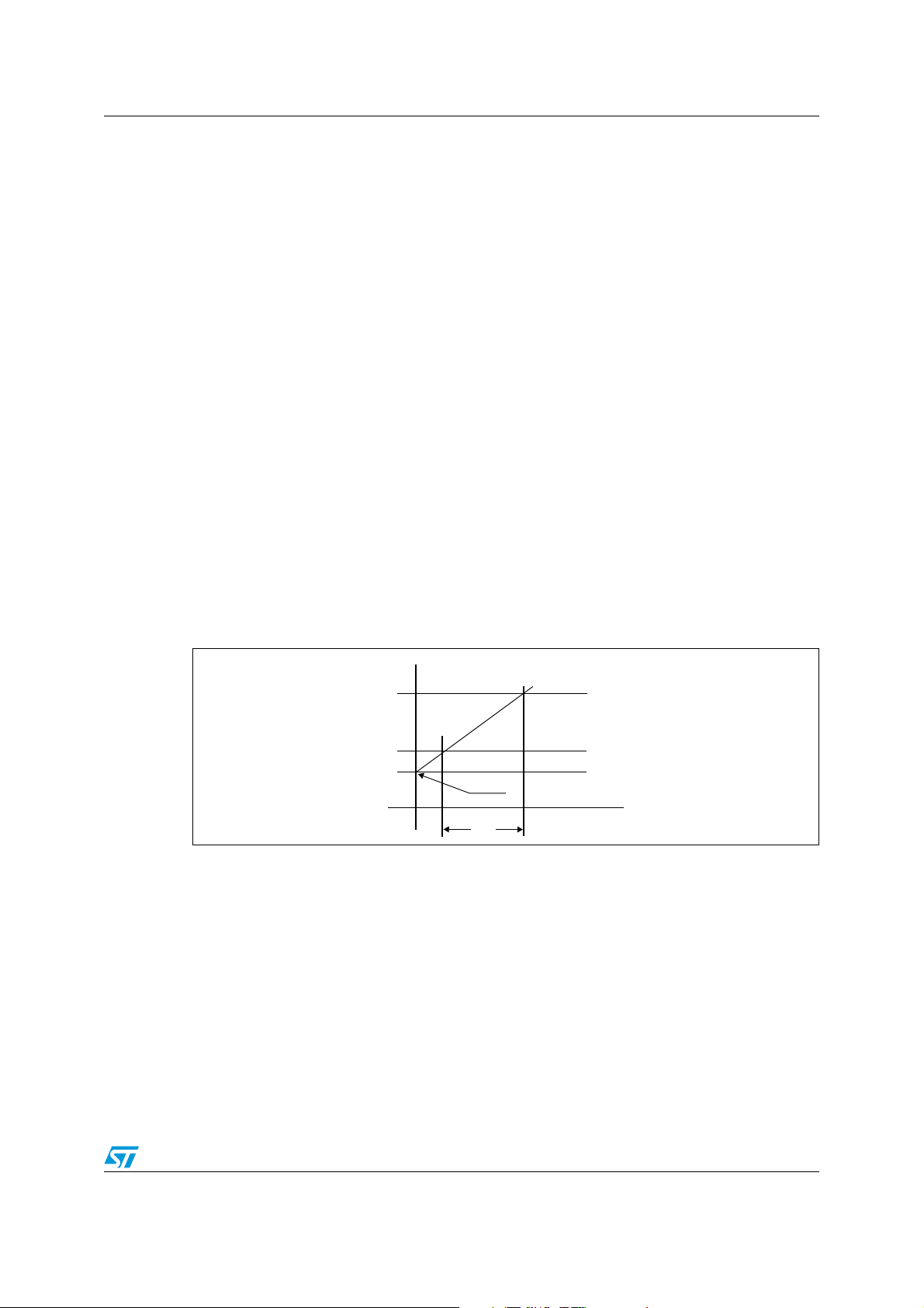
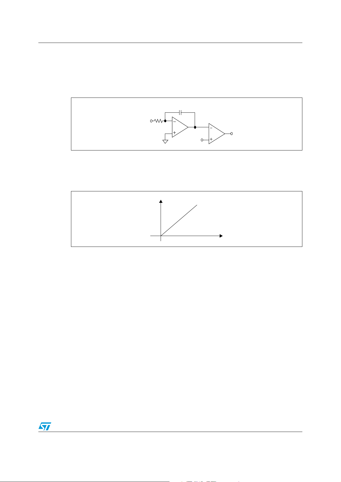
The purpose of using the second comparator (comp2) can be understood from the diagram below (Figure 2), which shows the relationship between the op-amp output (Amp in

Figure 1: Circuit diagram on page 6) and the time for a given input value.

Figure 2. Relationship between Vout and time for a given input

Vout

V3
V2
V1
	Point of
	uncertainty
T2	T3	Time (t)
	Tm

The time is measured as the difference of the two timer readings (T3 -T2) for the same slope. So factors like the residual voltage of the capacitor ( Vc(0+)) and any other constant errors (like the effect of output offset voltage) on the output side of the op-amp are subtracted. So its performance is better than a single-slope converter.

7/37

Timing diagram	AN2615

3 Timing diagram

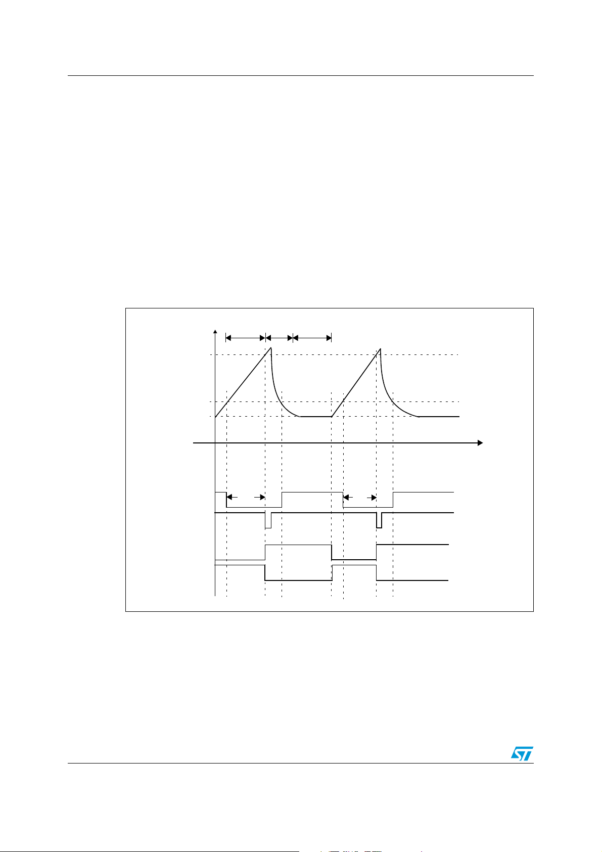
Figure 3 shows the overall operation of the ADC. Initially the capacitor is in the reset state

(M1on and M2off), the op-amp output Vout is at V1 and so, the output of both comparators, Comp1 and Comp2 is high.

Capacitor charging can be started by switching M1 - off and M2 - on. When the charging starts, Vout rises. When Vout becomes greater than V2, a falling edge occurs on Comp1. This causes an input capture at pin PB2 and software reads the timer value T2.

When Vout becomes greater than V3, a falling edge occurs on Comp2. Again this causes an input capture at pin PB0 and software reads the timer value T3.

The capacitor is discharged by switching M1 - on and M2off. After this, the ADC can be kept in reset condition by switching M1 - on and M2 - off or we can continue repeating the same process and make more measurements.

Figure 3. Timing diagram

	Charging	Discharg.	Settling
	time	time	time
V3
Vout
V2
V1
0	T2	T3	Time (t)
Comp1	Tm		Tm
	Tm		Tm
Comp2
M1
M2

8/37

AN2615	Circuit analysis

4 Circuit analysis

In this analysis, it is assumed that there is no noise present and the i/p offset voltage of the op-amp is negligible.

I = (V1 – Vin)/R = C * dVc/dt
Where, Vc = Vout – V1 and current ‘I’ is constant for a given input.
Applying the Laplace transform:
(V1 – Vin)/s * R = C * (s Vc(s) – Vc (0+))
or,
(V1 – Vin)/s2 = (R * C) * ( Vc (s) - Vc(0+)/s)
Applying the inverse Laplace transform, we get
(V1 – Vin) * T = (R * C) * ( Vc(t) - Vc(0+) ) -------------------	(1)
As shown in Figure 3: Timing diagram on page 8
At T = T2, Vc(T2) = V2 – V1
And, at T =T3, Vc (T3)= V3 – V1
So,
(V1 – Vin) * T2 = (R * C) * (V2 – V1 - Vc(0+)) -------------------	(2)
And,
(V1– Vin) * T3 = (R * C) * (V3 – V1 - Vc(0+)) -------------------	(3)

Equation (2) and equation (3) can both be used as the characteristic equation for this converter, but factors like Vc(0+) and other constant errors remain present. But if we use both comparators, then we can remove these factors by subtracting equation (2) and equation (3).

After subtracting equation (2) from equation (1) and rearranging we get:

Vin = V1 - (R * C) *( V3 – V2 )/(T3 –T2) -------------------	(4)
Let measured time T3 - T2 = Tm and we get:
Vin = V1 - (R * C) * ( V3 – V2 )/Tm -------------------	(5)

By using equation (5) we can measure the value of Vin depending on the value of T3 and T2.

9/37

Vout vs time diagram for different input voltages

AN2615

5 Vout vs time diagram for different input voltages

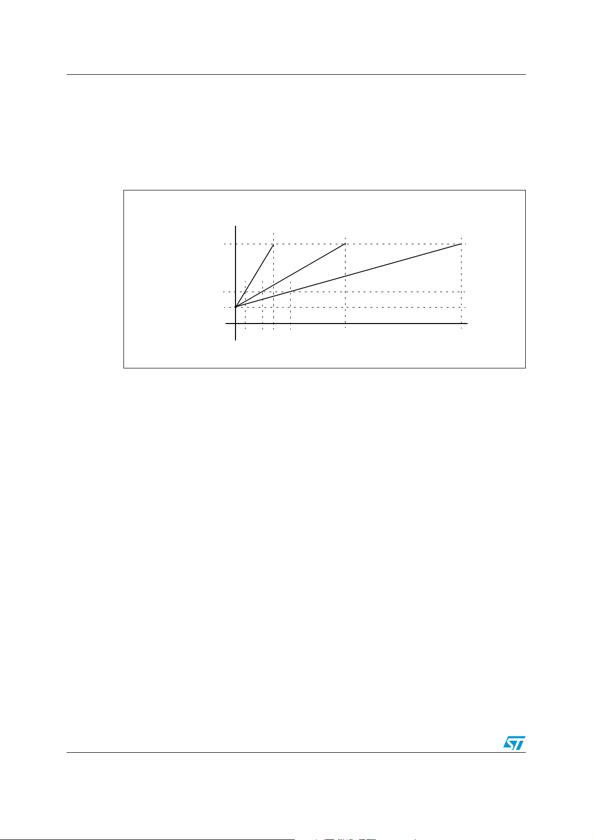
In Figure 4, we can see the relationship between the Vout and time for different input voltages. From the figure, it is clear that the conversion time for a negative input voltage is less than the time taken for a positive input voltage.

Figure 4. Vout vs time for different input voltages

Effective time Tm = T - T’
V3	Vin < 0	Vin =0	Vin > 0
	Vin < 0	Vin =0	Vin > 0

Vout
V2
V1

	T1’ T2’ T1 T3’	T2	T3
		Time (t)

1.Tm1: for Vin < 0; Tm2: for Vin = 0; and Tm3: for Vin > 0 (where Tin1 < Tin2 < Tin3)

2.This ADC works for the range Vin <= V1 but if the input voltage is greater than V1 the direction of current I is inverted and the capacitor starts charging in the opposite direction and conversion never takes place.

3.For negative voltage currents I, that depend on the difference V1 - Vin, is high, so the charging time for negative voltages is less than the positive voltages.

10/37

AN2615	Characteristics of different slope converters

6 Characteristics of different slope converters

6.1Single-slope converter

Figure 5. Single-slope converter circuit diagram

-Vref

VINT

Vin

6.1.1Single-slope converter timing diagram

Here Vin is directly proportional to the time measured.

Figure 6. Single-slope converter timing diagram

Vin

Time

1. Here Vin = K * Tm

The major sources of conversion errors are the correction factor for the R*C product and the input offset voltage.

A single-slope converter requires a dual supply voltage op-amp to be able to measure the positive and negative voltages.

11/37

Characteristics of different slope converters	AN2615

6.2Dual-slope converter

Figure 7. Dual-slope converter circuit diagram

Control logic

-Vin

Vref

out

1 out

cmp

ctr

enbl

gnd

clk

Counter

clk

6.2.1Dual-slope converter timing diagram

As shown in Figure 8 a dual-slope ADC has a charging phase followed by a fixed rate discharging phase.

Figure 8. Dual-slope converter timing diagram

Charging phase	Fixed-rate discharge
Vin1	-Vref	Vin	=	Tcharge
		Vref		Tdischarge
Vin2	-Vref

Time

The advantage of a dual-slope ADC is that it is not dependent on the correction factor for the R*C product. However, the input offset voltage problem still persists and this ADC also requires a dual supply op-amp to be able to measure positive and negative voltages.

12/37

+ 25 hidden pages