ST AN2388 Application note

AN2388

Application note

Sensor field oriented control (IFOC)

of three-phase AC induction motors using ST10F276

Introduction

AC Induction motors are the most widely used motors in industrial motion control systems,
as well as in home appliances thanks to their reliability, robustness and simplicity of control.

Until a few years ago the AC motor could either be plugged directly into the mains supply or
controlled by means of the well-known scalar V/f method. When power is supplied to an
induction motor at the recommended specifications, it runs at its rated speed. With this
method, even simple speed variation is impossible and its system integration is highly
dependent on the motor design (starting torque vs maximum torque, torque vs inertia,
number of pole pairs). However many applications need variable speed operation. The
scalar V/f method is able to provide speed variation but does not handle transient condition
control and is valid only during a steady state. This method is most suitable for applications
without position control requirements or the need for high accuracy of speed control and
leads to over-currents and over-heating, which necessitate a drive which is then oversized
and no longer cost effective. Examples of these applications include heating, air
conditioning, fans and blowers.

During the last few years the field of electrical drives has increased rapidly due mainly to the
advantages of semiconductors in both power and signal electronics and culminating in
powerful microcontrollers and DSPs. These technological improvements have allowed the
development of very effective AC drive control with lower power dissipation hardware and
increasingly accurate control structures. The electrical drive controls become more accurate
with the use of three-phase currents and voltage sensing.

This application note describes the most efficient scheme of vector control: the Indirect Field
Oriented Control (IFOC). Thanks to this control structure, the AC machine, with a
speed/position sensor coupled to the shaft, acquires every advantage of a DC machine
control structure, by achieving a very accurate steady state and transient control, but with
higher dynamic performance.

In this document we will look at the complete software integration and also the theoretical
and practical aspects of the application.

October 2006 Rev 1 1/54

www.st.com

Contents AN2388

Contents

1 Background . . . . . . . . . . . . . . . . . . . . . . . . . . . . . . . . . . . . . . . . . . . . . . . . 4

1.1 AC induction motor . . . . . . . . . . . . . . . . . . . . . . . . . . . . . . . . . . . . . . . . . . . 4

1.1.1 Stator . . . . . . . . . . . . . . . . . . . . . . . . . . . . . . . . . . . . . . . . . . . . . . . . . . . . 4

1.1.2 Rotor . . . . . . . . . . . . . . . . . . . . . . . . . . . . . . . . . . . . . . . . . . . . . . . . . . . . 5

1.2 Three-phase induction motor and classical AC drives . . . . . . . . . . . . . . . . 6

2 Vector control of AC induction machines . . . . . . . . . . . . . . . . . . . . . . . . 9

2.1 Introduction . . . . . . . . . . . . . . . . . . . . . . . . . . . . . . . . . . . . . . . . . . . . . . . . 9

2.2 Theory on vector control . . . . . . . . . . . . . . . . . . . . . . . . . . . . . . . . . . . . . . 9

2.2.1 Space vector definition and projection . . . . . . . . . . . . . . . . . . . . . . . . . . 10

2.2.2 The (a,b,c)(α,β) projection (Clark transformation) . . . . . . . . . . . . . . . . . 11

2.2.3 The (α,β)(d,q) projection (Park transformation) . . . . . . . . . . . . . . . . . . . 12

2.2.4 The (d,q)(α,β) projection (inverse Park transformation) . . . . . . . . . . . . . 13

2.3 Block diagram of the vector control . . . . . . . . . . . . . . . . . . . . . . . . . . . . . 14

2.4 The current model (rotor flux estimator) . . . . . . . . . . . . . . . . . . . . . . . . . . 14

2.5 Space vector modulation (SVPWM) . . . . . . . . . . . . . . . . . . . . . . . . . . . . . 16

3 Hardware design . . . . . . . . . . . . . . . . . . . . . . . . . . . . . . . . . . . . . . . . . . . 22

3.1 System configuration . . . . . . . . . . . . . . . . . . . . . . . . . . . . . . . . . . . . . . . . 22

3.2 MDK-ST10 control board . . . . . . . . . . . . . . . . . . . . . . . . . . . . . . . . . . . . . 22

3.3 Three-phase high voltage power stage (powerBD-1000) . . . . . . . . . . . . . 23

3.3.1 Power stage . . . . . . . . . . . . . . . . . . . . . . . . . . . . . . . . . . . . . . . . . . . . . . 24

3.3.2 Auxiliary supply . . . . . . . . . . . . . . . . . . . . . . . . . . . . . . . . . . . . . . . . . . . 25

3.4 Gate driver board . . . . . . . . . . . . . . . . . . . . . . . . . . . . . . . . . . . . . . . . . . . 26

3.5 Current sensing board . . . . . . . . . . . . . . . . . . . . . . . . . . . . . . . . . . . . . . . 29

3.6 The 3-phase AC induction motor . . . . . . . . . . . . . . . . . . . . . . . . . . . . . . . 30

4 Software design . . . . . . . . . . . . . . . . . . . . . . . . . . . . . . . . . . . . . . . . . . . . 32

4.1 Introduction . . . . . . . . . . . . . . . . . . . . . . . . . . . . . . . . . . . . . . . . . . . . . . . 32

4.2 Software organization . . . . . . . . . . . . . . . . . . . . . . . . . . . . . . . . . . . . . . . . 32

4.3 Software variables . . . . . . . . . . . . . . . . . . . . . . . . . . . . . . . . . . . . . . . . . . 35

4.4 Base values and PU model . . . . . . . . . . . . . . . . . . . . . . . . . . . . . . . . . . . 36

4.4.1 Magnetizing current . . . . . . . . . . . . . . . . . . . . . . . . . . . . . . . . . . . . . . . 36

2/54

AN2388 Contents

4.4.2 Numerical considerations . . . . . . . . . . . . . . . . . . . . . . . . . . . . . . . . . . . 37

4.4.3 ST10-DSP features . . . . . . . . . . . . . . . . . . . . . . . . . . . . . . . . . . . . . . . . 37

4.5 Analog value scaling . . . . . . . . . . . . . . . . . . . . . . . . . . . . . . . . . . . . . . . . 39

4.5.1 Current sensing and scaling . . . . . . . . . . . . . . . . . . . . . . . . . . . . . . . . . 39

4.5.2 Rotor mechanical position sensing . . . . . . . . . . . . . . . . . . . . . . . . . . . . 40

4.5.3 The PI regulator . . . . . . . . . . . . . . . . . . . . . . . . . . . . . . . . . . . . . . . . . . . 43

4.6 Clark and Park transformation . . . . . . . . . . . . . . . . . . . . . . . . . . . . . . . . . 44

4.6.1 (a,b)->(α,β) projection (Clark transformation) . . . . . . . . . . . . . . . . . . . . 44

4.6.2 The (α,β)-> (d,q) projection (Park transformation) . . . . . . . . . . . . . . . . . 45

4.6.3 The Current model implementation (rotor flux estimator) . . . . . . . . . . . 45

4.6.4 Generation of sine and cosine values . . . . . . . . . . . . . . . . . . . . . . . . . . 46

4.6.5 The space vector modulation module . . . . . . . . . . . . . . . . . . . . . . . . . . 47

5 References . . . . . . . . . . . . . . . . . . . . . . . . . . . . . . . . . . . . . . . . . . . . . . . . 52

6 Revision history . . . . . . . . . . . . . . . . . . . . . . . . . . . . . . . . . . . . . . . . . . . 53

3/54

Background AN2388

1 Background

1.1 AC induction motor

The AC induction motor is a rotating electric machine designed to operate from a 3-phase
source of alternating voltage. Asynchronous motors are based on induction. The cheapest
and most widely used is the squirrel cage motor in which aluminum conductors or bars are
cast into slots in the outer periphery of the rotor. These conductors or bars are shorted
together at both ends of the rotor by cast aluminum end rings. For variable speed drives, the
source is normally an inverter that uses power switches to produce approximately sinusoidal
voltages and currents controllable in terms of frequency and magnitude.

Like most motors, an AC induction motor has a fixed outer portion, called the stator and a
rotor that spins inside with a well-optimized air gap between the two.

Virtually all electrical motors use magnetic field rotation to spin their rotors. A three-phase
AC induction motor is the only type where the rotating magnetic field is generated naturally
in the stator because of the nature of the supply.

In an AC induction motor, one set of electromagnets is formed in the stator because the AC
supply is connected to the stator windings. The alternating nature of the supply voltage
induces an Electromagnetic Force (EMF) in the rotor (just like the voltage is induced in the
secondary transformer) as per Lenz’s law, thus generating another set of electromagnets;
hence the name “induction motors”.

Interaction between the magnetic field of these electromagnets generates a revolving force,
or torque. As a result, the motor rotates in the direction of the resultant torque.

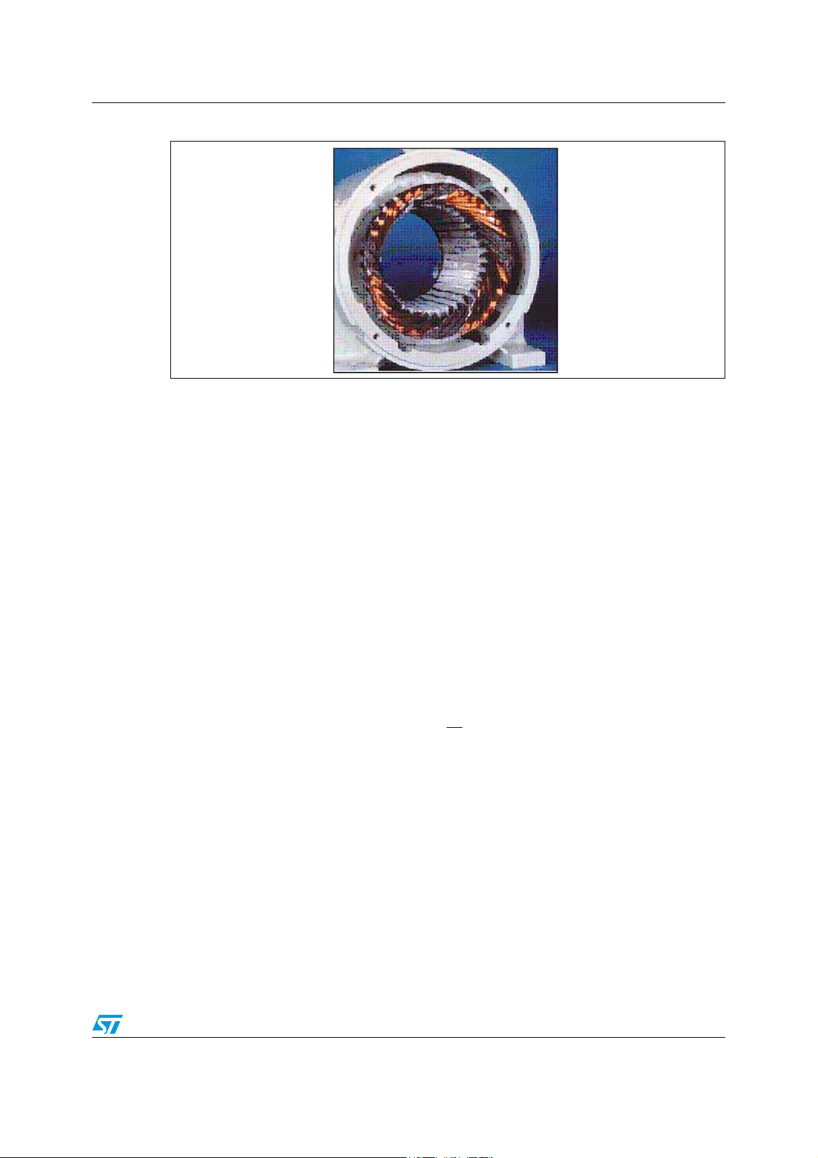
1.1.1 Stator

The stator is made up of several thin laminations of aluminum or cast iron. They are
punched and clamped together to form a hollow cylinder (stator core) with slots as shown in

Figure 1. Coils of insulated wires are inserted into these slots. Each grouping of coils,

together with the core it surrounds, forms an electromagnet (a polar pair) on the application
of AC supply.

The number of poles of an AC induction motor depends on the internal connection of the
stator windings. Internally they are connected in such a way, that when an AC supply is
applied, a rotating magnetic field is created.

4/54

AN2388 Background

Figure 1. Stator core and windings

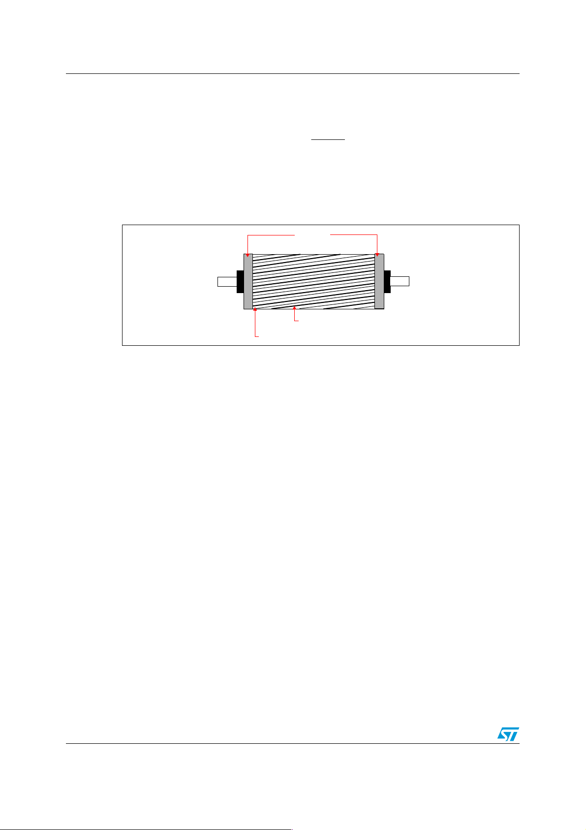
1.1.2 Rotor

The rotor is made up of several thin steel laminations with spaced bars, which are made up
of aluminum or copper, along the periphery. In the most popular type of rotor (squirrel cage
rotor), these bars are connected mechanically at the ends and electrically by the use of
rings. The rotor consists of a cylindrical laminated core with an axially placed parallel slot for
carrying the conductors. Each slot carries a copper, aluminum or alloy bar. These rotor bars
are permanently short-circuited at both ends by means of the end rings. The rotor slots are
not exactly parallel to the shaft in order to decrease magnetic hum and slot harmonics.
Moreover this reduces the locking tendency of the rotor. In fact, the rotor teeth tend to
remain locked under the stator teeth due to direct magnetic attraction between the two. This
happens when the number of stator teeth are equal to the number of rotor teeth.

The rotor is mounted on the shaft using bearings on each end. One end of the shaft is
usually kept longer than the other for driving the load. Some motors may have
position/speed sensing devices. Between the stator and the rotor exists an air-gap, through
which, due to induction, the energy is transferred from the stator to the rotor like a
transformer. The generated torque forces the rotor and then the load to rotate.

The magnetic field created in the stator rotates at a synchronous speed (N

N ×= 60

s

where:

N

= synchronous speed in RPM

s

= the number of pole pairs

p

p

f = the supply frequency in Hertz

f

p

p

).

s

The magnetic field produced in the rotor is alternating in nature because of the induced
voltage. The frequency of the induced EMF is the same as the supply frequency. Its
magnitude is proportional to the relative velocity between synchronous speed (stator
frequency) and rotor speed. Since the rotor bars are shorted at the ends, the EMF induced
produces a current in the rotor conductors.

When the magnetic field is generated the rotor starts to run in the same direction trying to
reach the same speed. The rotor revolves slower than the speed of the stator field. This
difference is called slip (s). The slip varies with the load so that an increasing of the load

5/54

Background AN2388

causes the rotor to slow down (or slip increasing). On the contrary, a decreasing of the load
causes the rotor to speed up (or slip decreasing). The slip is expressed as a percentage and
can be determined with the following formula:

−

NN

rs

=

Slip

where;

N

= synchronous speed in RPM

s

N

= rotor speed in RPM

r

100% ×

N

s

Figure 2. Rotor structure

Rings

Shaft

Conductors

Skewed slots

Slots in the inner periphery of the stator accommodate 3-phase winding a, b, c. The turns in
each winding produces an approximately sinusoidally-distributed flux density around the
periphery of the air gap. When three currents that are sinusoidally varying in time, but
displaced in phase by 120° from each other, flow through the three symmetrically placed
windings, a radially directed air gap flux density is produced that is also sinusoidally

distributed around the gap and rotates at an angular velocity equal to the angular frequency

ω

of the stator currents.

s

The flux produced by the stator current is a sinusoidally-distributed wave. This flux revolves
and collides with the rotor bars, generating rotor current in the short-circuited rotor bars.
Because of the low resistance of these shorted bars, only a small relative angular velocity ω
between the angular velocity ω

of the flux wave and the mechanical angular velocity ω of

s

the two pole rotor is required to produce the necessary rotor current.

The relative angular velocity ω

is called the slip velocity. The interaction of the sinusoidally

r

distributed air gap flux density and induced rotor currents produces a torque on the rotor.

1.2 Three-phase induction motor and classical AC drives

Three-phase AC induction motor are widely used in many fields. They are classified in two
categories:

● Squirrel cage motor

● Wound-rotor motor

90% of the three-phase AC Induction motors are squirrel cage motors because of their lower
cost and the possibility of starting heavier loads with respect to wound-rotor motors. The
range of power ratings goes from one-third to hundred horsepower.

r

The wound-rotor motor is a variation of the squirrel cage induction motor. While the stator is
the same as that the squirrel cage, it has a set of windings on the rotor which are not short-

6/54

AN2388 Background

circuited, but are terminated to a set of slip rings. These are helpful in adding external
resistors and contactors.

In fact, it is possible to demonstrate that the slip frequency producing the maximum torque
(pull-out torque) is directly proportional to the rotor resistance. In wound-rotor motors, the
real rotor resistance can be increased by connecting external resistors through the slip
rings. This possibility allows for higher slip and hence, the pull-out torque at lower speed. A
particularly high resistance can deliver a high pull-out torque starting from zero speed. As
the motor accelerates, the value of the resistance can be reduced so that the motor
characteristic can follow the load requirement at different speeds. Once the motor reaches
the nominal speed, external resistors are removed from the motor coming back to work as
the standard induction motor.

This motor type (when external resistors are connected with the rotor) is ideal for very high
inertia loads, where it is necessary to generate the pull-out torque at almost zero speed and
accelerate to full speed in the minimum time with minimum current consumption.

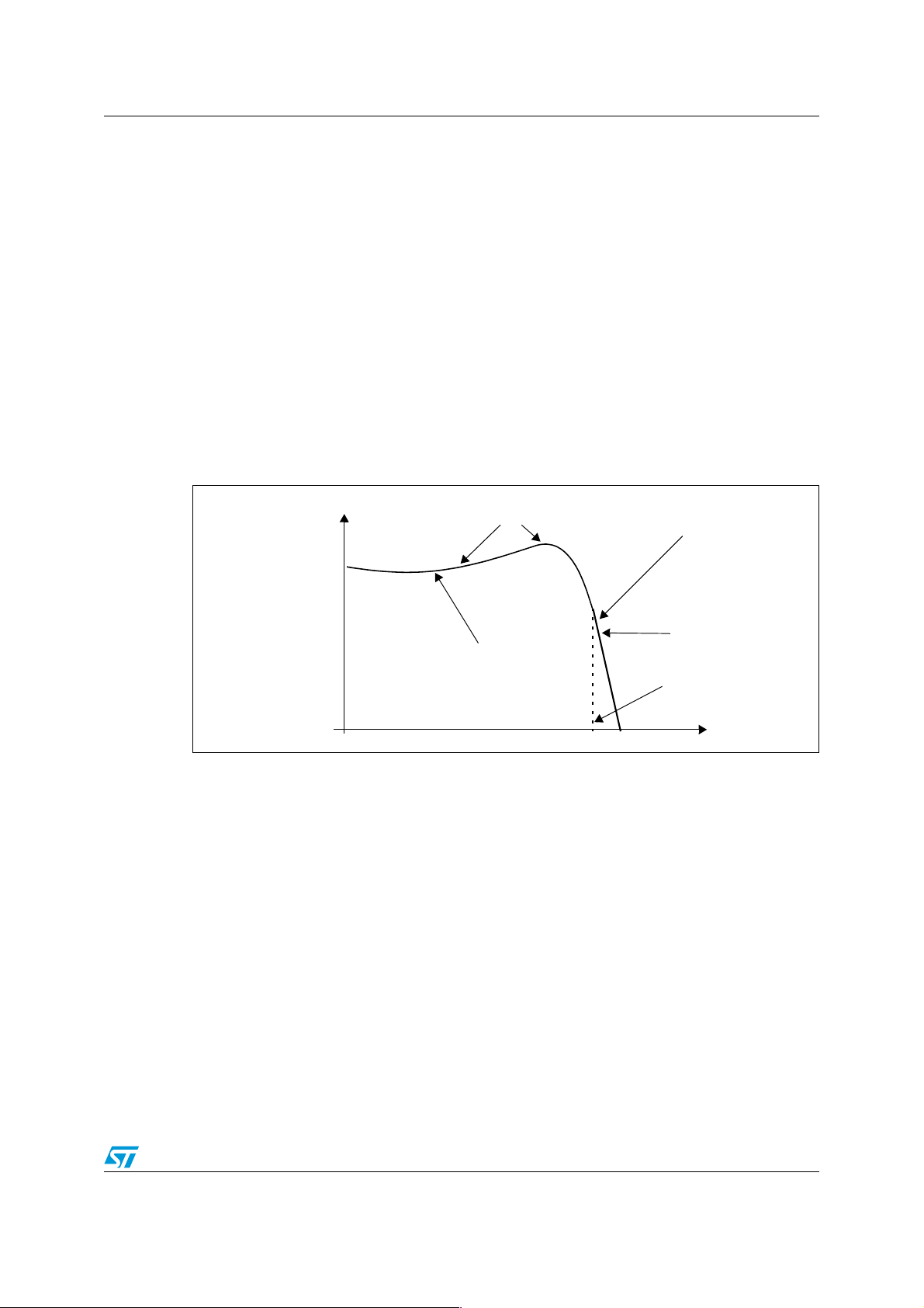
The typical speed-torque characteristic of an induction motor is shown in Figure 3

Figure 3. Speed-torque characteristic

Pull-out Torque

Locked Rotor Torque (LRT)

1.5

Flux decreases

Stable zone

T, r a t e d

1.0

Unstable points

Slip Speed

Flux = rated

Rotor speed

Nb Ns

The X axis shows speed and slip. The Y axis shows the torque. During start-up the motor
needs seven times the rated current and this depends on the interaction between stator and
rotor flux, the losses in the stator and rotor windings and losses in the bearing due to friction.
This over-current produces the torque necessary to spin the motor from zero speed.

During start-up, the motor is able to delivers 1.5 times the rated torque. This torque is called
locked rotor torque (LRT). Once the speed increases, the current that flows in the motor
reduces slightly. When the motor runs at approximately 80% of the synchronous speed, the
load can increase up to 2.5 times the rated torque. Any further growth in term of load could
take the motor to a stall condition.

As seen in the speed-torque characteristics, torque is highly nonlinear as the speed varies.
In all applications where it is necessary to regulate the speed a control strategy must be
used which is able to vary the frequency. One of the best known strategies is the simple
open loop method called Variable Voltage Variable Frequency or simply V/f method. This
method doesn’t allow management of the quantities in terms of phase but modifies only the
magnitude of the stator flux.

7/54

Background AN2388

φ

The torque delivered by the motor is directly proportional to the magnetic field produced by
the stator. The flux produced by the stator is proportional to the ratio of applied voltage and
frequency of the supply. By varying the frequency it is possible to control the speed motor.

If the ratio of voltage to frequency is kept constant, the torque delivered by the motor
remains constant under the condition of no torque load variation.

[][ ]

=∝

e

fVelocityAngularStatorFluxVVoltageStator

πφωφ

2*)(*)()(

or

V

=

f

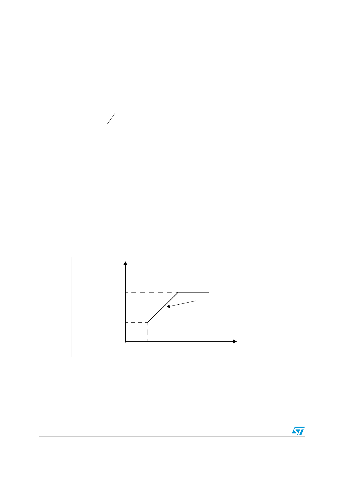
Figure 4 shows the relation between the voltage and torque versus frequency. At base

speed, the voltage and frequency reach their nominal values. The motor can be driven
beyond base speed by increasing the frequency. The applied voltage cannot be increased
beyond the V

voltage. Only the frequency can be increased. Above base speed losses,

max

mechanical friction and other complex factors increase significantly. The torque curve
becomes nonlinear respect to speed or frequency.

The Voltage on frequency is based on steady-state characteristics of the motor and the
assumption that the stator voltages and currents are sinusoidal. Its field of application is the
majority of existing variable-speed AC drives by means of an open-loop constant V/f voltage
source converter. No inner current controllers are required. The advantages of this control
technique is its simplicity, it is quick and easy to program and doesn’t require any highly
complex calculations.

The major drawback is the high reaction time for load variations and the efficiency during
these operation points. This is the reason why it is often used in fans and pumps where the
torque load is approximately constant.

Figure 4. Voltage frequency characteristic

Vs

Vmax

φ = constant

Vmin

f

minimum frequency rated frequency (stator frequency)

8/54

AN2388 Vector control of AC induction machines

2 Vector control of AC induction machines

2.1 Introduction

The performance of an AC induction motor is strongly dependant on its control. The recent
advances of powerful microcontrollers with DSP functions has enhanced complex and real­time algorithms. In particular, the use of a powerful microcontroller brings the following:

● system cost reduction by an efficient control and right dimensioning power devices as

well

● the removal of speed or position sensors by the implementation of sensorless

algorithms that need higher complexity calculations

● a reduction of current harmonics using enhanced algorithms

● a reduction in the number of look-up tables which reduces the amount of memory

required

● real-time generation of torque and flux profiles and move trajectories, resulting in

better-performance

Thanks to the capability of such modern microcontrollers it is possible to implement
sophisticated controls like Vector Control.

Vector control refers not only to the magnitude but also to the phase of variables. Matrix and
vectors are used to represent the control quantities. This method takes into account not only
successive steady-states but real mathematical equations that describe the motor itself, so
that the obtained results have a better dynamic for torque variations in a wider speed range.

The Field Oriented Control (FOC) offers a solution to circumvent the need to solve high
order equations with a large number of variables and nonlinearities and achieve an efficient
control with high dynamic.

This approach needs more calculations than other standard control schemes and has the
following advantages:

● full motor torque capability at low speed

● better dynamic behavior

● higher efficiency for each operation point in a wide speed range

● decoupled control of torque and flux

● short term overload capability

● four quadrant operation

2.2 Theory on vector control

FOC involves controlling the components of the motor stator currents, represented by a
vector, in a rotating reference frame (with a d-q coordinate system). In a special reference
frame, the expression for the electromagnetic torque of the smooth-air-gap machine is
similar to the expression for the torque of the separately excited DC machine. In the case of
induction machines, the control is normally performed in a reference frame aligned to the
rotor flux space vector. To perform the alignment on a reference frame revolving with the
rotor flux requires information on the modulus and the space angle (position) of the rotor flux

9/54

Vector control of AC induction machines AN2388

space vector. In order to estimate the rotor flux vector is possible to use two different
strategies:

● DFOC (Direct Field Oriented Control): rotor flux vector is either measured by means of

a flux sensor mounted in the air-gap or measured using the voltage equations starting
from the electrical machine parameters.

● IFOC (Indirect Field Oriented Control): rotor flux vector is estimated using the field

oriented control equations (current model) requiring a rotor speed measurement.

The usual terminology “Sensorless” specifies that no position/speed feedback devices are
used.

With these algorithms, the stator currents of the induction machine are separated into flux
and torque producing components by utilizing transformation to the d-q coordinate system.
On this reference frame the torque component is on the q axis and the flux component is on
the d axis. The vector control system requires the dynamic model equations of the induction
motor and returns to the instantaneous currents and voltages in order to calculate and
control the variables.

The technique described in this application note is IFOC. Indirect vector control of the rotor
currents can be implemented using the following data:

● Instantaneous stator phase currents, i

●

Rotor mechanical position

● Rotor electrical time constant

, ib, and i

a

c

The motor must be equipped with sensors to monitor the three-phase stator currents and a
rotor position feedback device. An encoder is normally mounted on the shaft rotor for this
purpose but in order to have a cheaper solution is possible to use a speed feedback device
such as a tachometer.

The key for understanding how vector control works is to explain the coordinate reference
transformation process. From the perspective of the stator, a sinusoidal input current is
forced to the stator. This time variant signal causes the generation of a rotating magnetic
flux. The speed of the rotor is a function of the rotating flux vector. From a stationary
perspective, the stator currents and motor and the rotating flux vector look like AC
quantities.

Keep in mind that the rotor flux speed is not equal to the revolving magnetic field, produced
by the stator phase windings, during the transient conditions. Looking at the motor from this
perspective during steady state conditions, the stator currents become constant.

2.2.1 Space vector definition and projection

The three-phase voltages, currents and fluxes of AC-motors can be deeply studied in terms
of complex space vectors. Assuming that i
phases we can define the stator current vector i

2

π

j

where and represent the spatial operators.

α

3

e=

α

4

π

j

2

3

e=

, ib, ic are the instantaneous currents in the stator

a

by:

s

2

iiii

αα

++=

cbas

This current space vector describes the three phase sinusoidal system.

10/54

AN2388 Vector control of AC induction machines

As discussed above, this three phase system can be transformed into a two time invariant
co-ordinate system. This transformation can be split in two steps:

● (a,b,c) -> (α,β) (the Clark transformation) which outputs a two co-ordinate time variant

system

● (α,β) -> (d,q) (the Park transformation) which outputs a two co-ordinate time invariant

system

2.2.2 The (a,b,c)(α,β) projection (Clark transformation)

The space vector can be reported in another reference frame with only two orthogonal axis
called (α, β). Assuming that the axis a and the axis α are in the same direction we have the
following vector diagram:

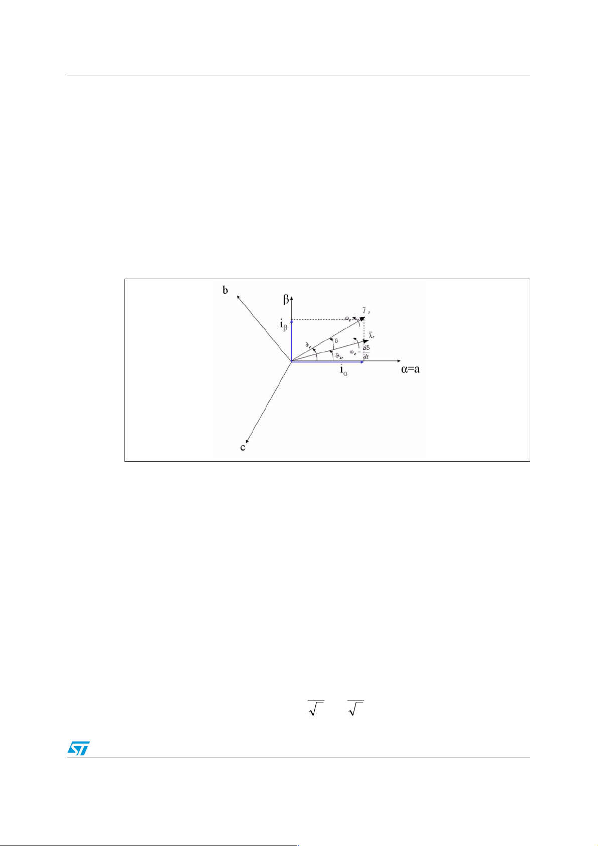
Figure 5. Stator space vector in 2-orthogonal axis (Clark components) in a

reference frame aligned with the stator

where:

θ

is the rotor flux position

λr

θ

is the revolving magnetic field position

e

ω

is the revolving magnetic field angular speed

e

δ is an angle that depends on torque load transitions

Take into consideration that δ doesn’t change in steady state so the rotor flux speed revolves
with the same speed of revolving magnetic field.

Basically the transformation moves from a 3-axis, 2-dimensional coordinate system
referenced to the stator of the motor to a 2-axis system also referenced to the stator.

The projection that modifies the three phase system into the (α,β) two-dimensional
orthogonal system is presented below.

ii

=

⎧

as

α

⎪
⎨

⎪
⎩

1

β

3

11/54

2

iii

+=

bas

3

Vector control of AC induction machines AN2388

We obtain a two co-ordinate system that still depends on time and speed.

Figure 6. Clark transformation module

i

⎛

⎞

s

⎜

⎟

⎜

⎟

i

βαs

⎝

⎠

ia

ib

Clarke

ic=-ia-ib

ialfa

ibeta

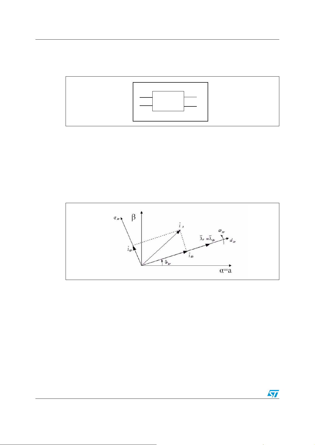
2.2.3 The (α,β)(d,q) projection (Park transformation)

This is the most important transformation in the FOC. In fact this projection modifies

a two phase orthogonal system (α,β) in the d, q rotating reference frame. Thanks to this
information it is possible to fix a component of the stato current on a d-axis responsible of
flux. If we consider the d-axis aligned with the rotor flux, the next diagram (Figure 7) shows,
for the current vector, the relationship from the two reference frames:

Figure 7. Stator Space vector in a reference frame revolving with the rotor flux

vector λ

r

where θλr is the rotor flux position. The flux and torque components of the current vector are
determined by the following equations:

⎧

⎪
⎨
⎪

⎩

These components depend on the current vector (α,β) components and on the rotor flux
position ; knowing the right rotor flux position, then make constant the d,q
component.

The two co-ordinate system obtained using a Park transformation has the advantages
of being time invariant and has separate torque and flux components for stator currents.

12/54

()

θ

r

λ

i

⎞

⎛

ds

⎟

⎜

⎟

⎜

i

qs

⎠

⎝

() ()

+=

iii

() ()

+−=

θθ

sincos

rsrsds

λβλα

iii

θθ

cossin

rsrsqs

λβλα

AN2388 Vector control of AC induction machines

Figure 8. Park transformation module

i

α

i

β

Rotor Flux Position

Park

θ

l

q

l

d

λ

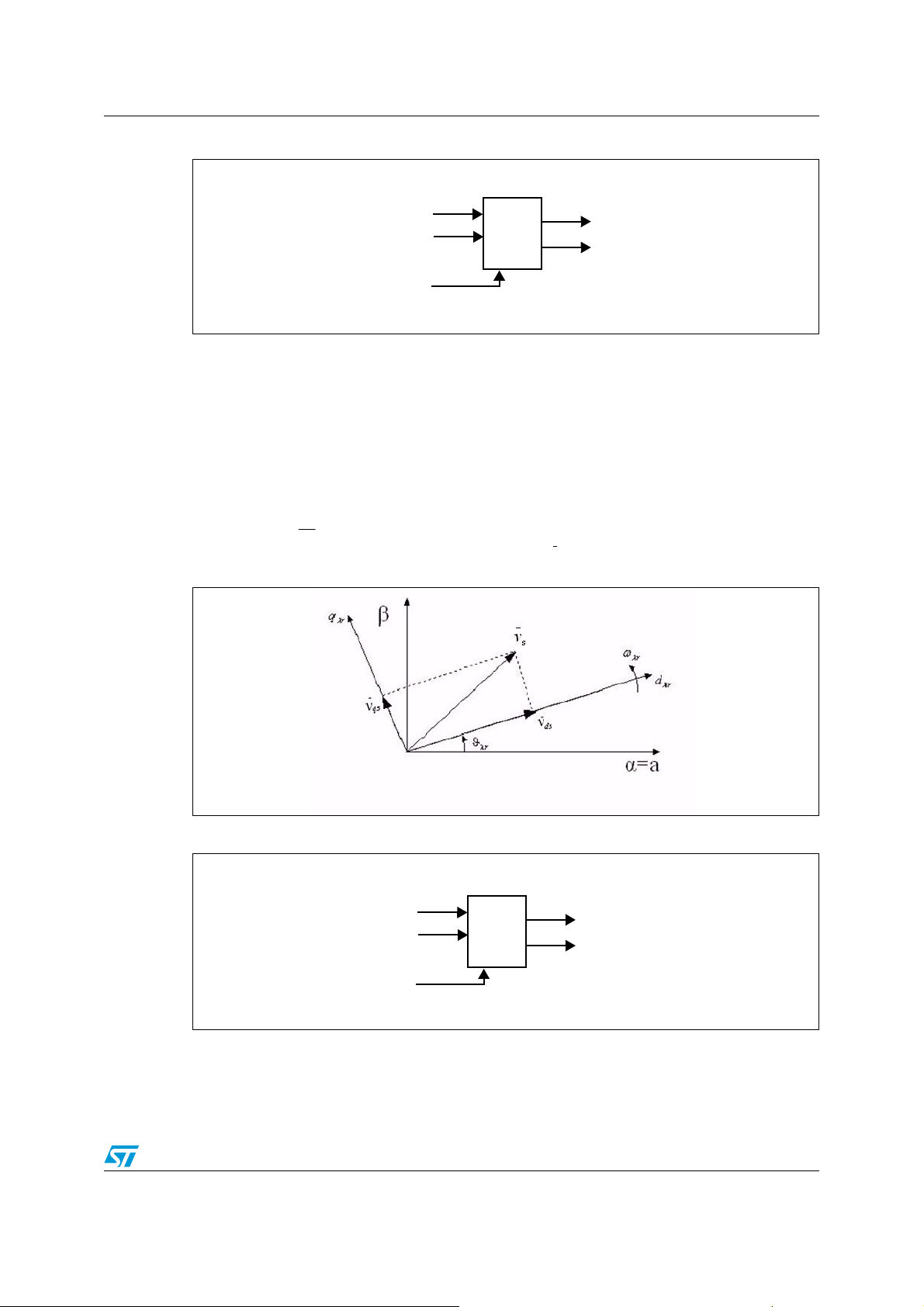
2.2.4 The (d,q)(α,β) projection (inverse Park transformation)

The equations presented here transform the stator voltage expressed in a d,q rotating
reference frame into a

The outputs of this block are the components of the reference vector to be applied to the
motor phases ( ) through space vector modulation.

V

(α,β) orthogonal system:

⎧

⎪
⎨
⎪

⎩

r

() ()

−=

VVV

() ()

−=

VVV

θθ

sincos

rqrefrdrefref

λλα

θθ

sinsin

rqrefrdrefref

λλβ

Figure 9. Voltage components in inverse Park transformation

Figure 10. Inverse Park transformation module

V

d

V

Inverse

q

Park

θ

r

λ

Rotor Flux Position

v

α

v

β

13/54

Vector control of AC induction machines AN2388

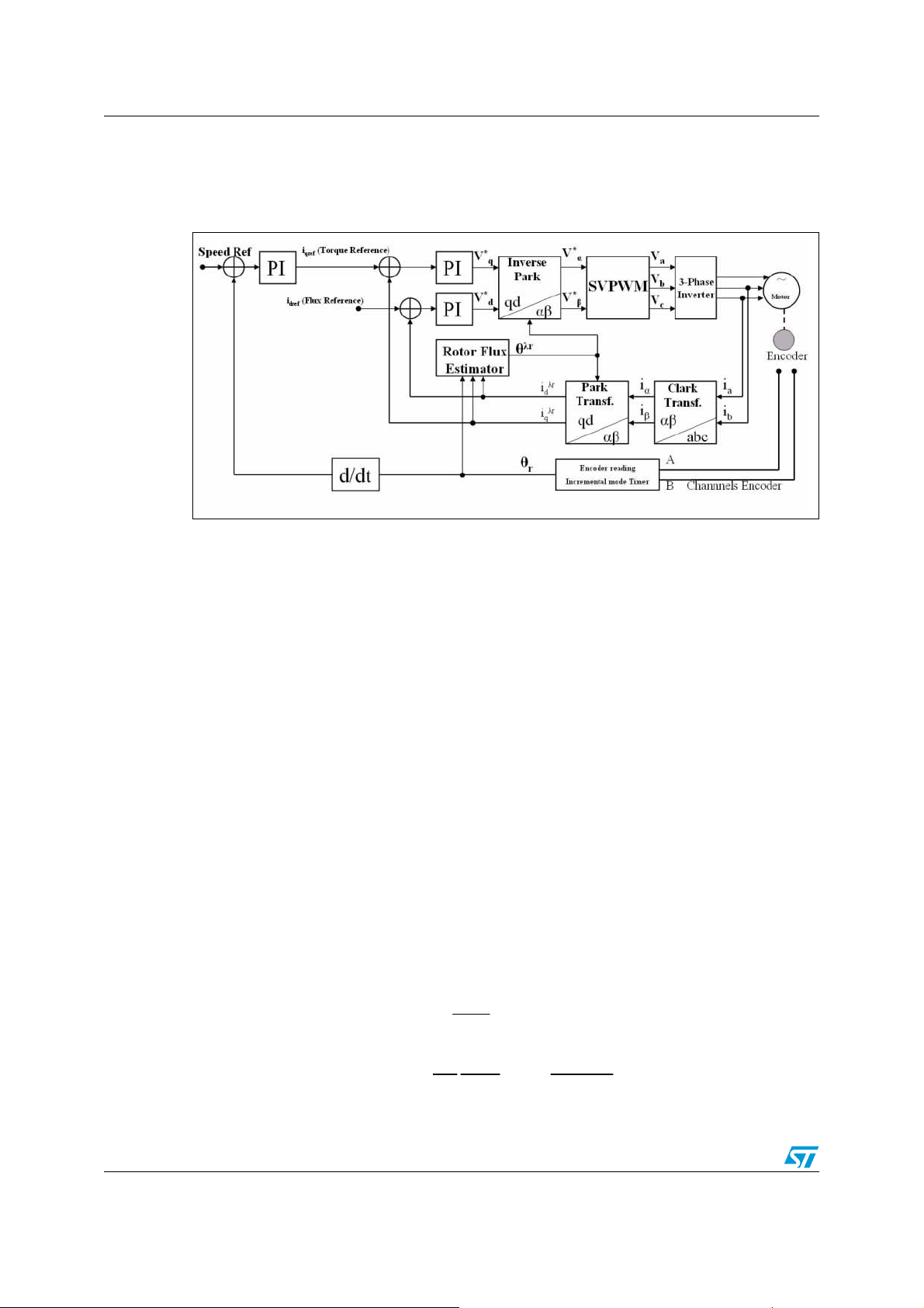
2.3 Block diagram of the vector control

The basic scheme of torque control with IFOC is shown below:

Figure 11. Block diagram of I.F.O.C.

Two phase currents go into some transformation module (Clarke and Park). The projection
outputs of the Clark block are indicated with i
current provide the input of the Park transformation that gives the current in the
reference frame aligned with the rotor flux vector. The exact rotor flux angular position (θ
is necessary to calculate the two components i
compared to the references i
torque command i
the right rotor flux command for every speed reference within the nominal value. The current
regulator outputs are V
transformation. The outputs of this are V
stator vector voltage in the α,β orthogonal reference frame. These are the inputs of the
Space Vector PWM. The outputs of this block are the gate signals that drive the inverter.
The main block of the vector control is the
resistance and rotor inductance as parameters and knowledge of these, with the highest
accuracy, greatly affects the performance of the control.

is the output of the speed regulator. The flux command i

qref

dref

(the flux reference) and i

dref

and V

. They are processed into the inverse Park

qref

αref

and isβ. These two components of the

sα

and i

ds

and V

Current Model block. This block needs the rotor

The ids and iqs components are

qs.

(the torque reference). The

qref

, which are the components of the

βref

d,q rotating

indicates

dref

λr

)

2.4 The current model (rotor flux estimator)

Knowledge of the rotor flux space vector magnitude and position are key for the AC
induction motor vector control. Knowing the rotor magnetic angular position allows to
establish, in fact, the rotational co-ordinate system (d, q). .

The current model consists of implementing the following two equations of the motor in the
d-q reference frame:

di

mR

+=

dt

d

θ

dt

i

mR

i

λ

r

n

qs

+==

iT

Ti

rds

1

f

s

ω

b

14/54

ω

bmRr

AN2388 Vector control of AC induction machines

L

where θλr is the rotor flux position, imR the magnetizing current and the rotor time

T =

constant.

r

r

R

r

The knowledge of this constant is critical for the proper functioning of the overall FOC since
it is strictly tied to the rotor flux speed that is integrated to get the rotor flux position.

Assuming the previous equation can be discretized as follows:

ii ≈

qSqS

+1

kK

mR

mR

+

T

k

T

r

1

+=

1

T

ω

ωθθ

r

λλ

k

−+=

mRds

KK

i

qs

K

i

mR

br

1

k

+

⋅⋅+=

sb

1

k

+

ii

k

1

+

nf

ks

k

1

+

r

k

1

+

eqii

eq

eqTf

1.)(

2.

3.

where:

i

= magnetizing current

mR

f

=rotor flux speed

s

T = sampling time

n = rotor mechanical speed

T

= Lr / Rr (Rotor time constant)

r

θλr = rotor flux position

ω

= electrical nominal flux speed

b

During the steady state condition, the Id current component is responsible for generating the
rotor flux. For transient changes, there is a low-pass filtered relationship between the
measured I
component of I

Under steady-state conditions, I

current component and the rotor flux. The magnetizing current, ImR, is the

d

that is responsible for producing the rotor flux.

d

is equal to ImR. This equation is dependent upon accurate

d

knowledge of the rotor electrical time constant.

Essentially, the equation of the magnetizing current corrects the flux producing component
of I

during transient changes.

d

The computed I
frequency is a function of the rotor electrical time constant, I

value is then used to compute the slip frequency (eq.2) The slip

mR

, ImR and the current rotor

q

velocity.

Equation 3 is the final flux estimator equation. It expresses the new flux angle based on the
slip frequency calculated in Equation 2 and the previously calculated flux angle.

If the slip frequency and stator currents have been related by Equation1 and Equation 2,
then motor flux and torque have been specified. Furthermore, these two equations ensure
that the stator currents are properly oriented to the rotor flux. If proper orientation of the
stator currents and rotor flux is maintained, then flux and torque can be controlled
independently. The I

current component controls motor torque. Already explained is the

d

principle of the indirect vector control.

15/54

Vector control of AC induction machines AN2388

2.5 Space vector modulation (SVPWM)

Space vector modulation is a sophisticated PWM method that provides advantages to the
application when compared to classical sinusoidal weighted modulation PWM:

● Higher bus voltage utilization (86%)

● Lower THD%

One common way to represent the phase voltages A, B, C is the space vector model. The
three legs of the three phase inverter can connect the phases of the motor to positive or
negative terminal of DC bus voltage. Considering that one and only one switch per leg must
be closed, 8 different states are possible. It is possible to associate a reference vector to
each of the 8 states. In order to generate a rotating field, the inverter has to be switched in
six of the eight states. This mode of operation is called six-step mode. The remaining two
states are called zero vectors because in these states the voltage applied in the motor
windings is null due to the middle point of each leg is connected to GND or to the DC bus
voltage. The zero vectors, located in the middle of the hexagon, see Figure 17, can be used
to regulate the amplitude of the space vector. The angle between any two vectors is 60°.

Note that whenever transistor T1 is on, transistor T2 is off, and vice versa. This makes it
easy to adopt a simple notation to describe the state of the inverter. For example, the state
when transistors T1, T4 and T6 are “on” (and of course T2, T3, and T5 are “off”) can be
represented with the notation (+,-,-). The state where transistors T2, T3, T6 are on is
denoted by (-, +, -).

Thanks to this notation is possible to determine the following states related to the power
switches of the inverter.

(+, -, -), (+, +, -), (-, +, -), (-, +, +), (-, -, +), (+, -, +),

Running the inverter through this switching sequence will produce the line-to-neutral
voltages shown in Figure 12.

16/54

AN2388 Vector control of AC induction machines

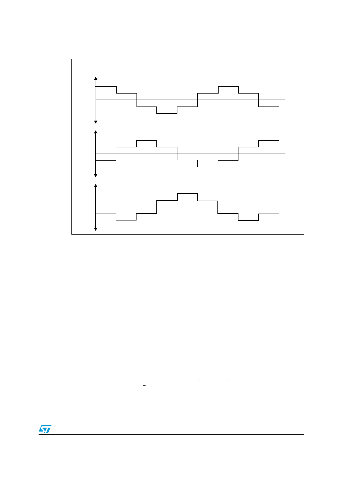
Figure 12. Line to neutral voltage in “six-step mode”

Van

(+,-,-) (+,+,-) (-,+,-) (-,+,+) (-,-,+) (+,-,+)

Vbn

(+,-,-) (+,+,-) (-,+,-) (-,+,+) (-,-,+) (+,-,+)

Vcn

(+,-,-) (+,+,-) (-,+,-) (-,+,+) (-,-,+) (+,-,+)

This strategy of operation is called “six-step mode”. Operating in this mode allows you to use
the full capabilities of the inverter. The amplitude of the fundamental frequency in six-step
mode is actually greater than the inverter rail voltage.

Space vector modulation uses six-step mode, but smoothes out the steps through some
sophisticated averaging techniques. For example, if a voltage is required between two step
voltages, the corresponding inverter states can be activated in such a way that the average
of the step voltages produces the desired output. To develop the equations needed to
generate this averaging effect, the problem is transformed into an equivalent geometrical
problem. The first step in this re-definition is to transform the inverter voltages of six-step
mode into a space vector.

Space vectors are similar to phasors and they are denoted by a magnitude and an angle. It’s
important to note that space vectors are not phasors. Phasors are used to represent a
single time varying sinusoid. Space vectors are used to represent three spatially separated
time variant quantities. If there are three time varying quantities, which sum to zero and are
spatially separated by 120°, then these quantities can be expressed as a single space
vector.

Since the three line-to-neutral voltages sum to zero, they can easily be converted into a
space vector (u

) using the following transformation:

s

⎛
⎜
⎜
⎝

0

j

an

bn

2

j

3

++=

2

−

j

⎞

3

⎟

)()()(

etVetVetVu

cn

⎟
⎠

Since the components of space vectors are projected along constant angles (0,-2π/3, and
2π/3), it is easy to graphically represent a space vector as shown in

Figure 14.

17/54