

Page 1

AN2290
Application note
Flux control simulink and software library of a PMSM
Introduction
This application note describes a software library for the electric motor control implementing
a (FOC) Flux Oriented Control on an ST10 microcontroller.
March 2007 Rev 1 1/53
www.st.com
Page 2

Contents AN2290
Contents
1 Introduction . . . . . . . . . . . . . . . . . . . . . . . . . . . . . . . . . . . . . . . . . . . . . . . . 6
2 FOC-flux oriented control . . . . . . . . . . . . . . . . . . . . . . . . . . . . . . . . . . . . . 7
2.1 PMSM . . . . . . . . . . . . . . . . . . . . . . . . . . . . . . . . . . . . . . . . . . . . . . . . . . . . . 8
2.2 Mathematical model of the machine . . . . . . . . . . . . . . . . . . . . . . . . . . . . . . 9
2.3 FOC control structure of PMSM . . . . . . . . . . . . . . . . . . . . . . . . . . . . . . . . 12
2.4 The space vector modulation theory . . . . . . . . . . . . . . . . . . . . . . . . . . . . 13
2.4.1 The 3-phase inverter . . . . . . . . . . . . . . . . . . . . . . . . . . . . . . . . . . . . . . . 14
2.4.2 The Space vector pulse width modulation . . . . . . . . . . . . . . . . . . . . . . . 15
2.4.3 Sector finder . . . . . . . . . . . . . . . . . . . . . . . . . . . . . . . . . . . . . . . . . . . . . 16
2.4.4 SVM formulation . . . . . . . . . . . . . . . . . . . . . . . . . . . . . . . . . . . . . . . . . . 17
3 Flux control simulink library . . . . . . . . . . . . . . . . . . . . . . . . . . . . . . . . . 20
3.1 Description . . . . . . . . . . . . . . . . . . . . . . . . . . . . . . . . . . . . . . . . . . . . . . . . 20
3.2 Using the simulink library . . . . . . . . . . . . . . . . . . . . . . . . . . . . . . . . . . . . . 20
3.2.1 How to install simulink library . . . . . . . . . . . . . . . . . . . . . . . . . . . . . . . . . 20
3.2.2 Test environment . . . . . . . . . . . . . . . . . . . . . . . . . . . . . . . . . . . . . . . . . . 21
3.3 Parameters format . . . . . . . . . . . . . . . . . . . . . . . . . . . . . . . . . . . . . . . . . . 21
3.4 Clarke transformation . . . . . . . . . . . . . . . . . . . . . . . . . . . . . . . . . . . . . . . . 22
3.5 Park transformation . . . . . . . . . . . . . . . . . . . . . . . . . . . . . . . . . . . . . . . . . 24
3.6 Inverse Park transformation . . . . . . . . . . . . . . . . . . . . . . . . . . . . . . . . . . . 26
3.7 Sin_cos . . . . . . . . . . . . . . . . . . . . . . . . . . . . . . . . . . . . . . . . . . . . . . . . . . 27
3.8 PI block . . . . . . . . . . . . . . . . . . . . . . . . . . . . . . . . . . . . . . . . . . . . . . . . . . . 28
3.9 SVM . . . . . . . . . . . . . . . . . . . . . . . . . . . . . . . . . . . . . . . . . . . . . . . . . . . . . 29
4 Flux control software library . . . . . . . . . . . . . . . . . . . . . . . . . . . . . . . . . 33
4.1 Description . . . . . . . . . . . . . . . . . . . . . . . . . . . . . . . . . . . . . . . . . . . . . . . . 33
4.2 Using the software library . . . . . . . . . . . . . . . . . . . . . . . . . . . . . . . . . . . . . 33
4.2.1 How to install Software library . . . . . . . . . . . . . . . . . . . . . . . . . . . . . . . . 33
4.2.2 Tool chain compatibility . . . . . . . . . . . . . . . . . . . . . . . . . . . . . . . . . . . . . 33
4.2.3 Calling a function . . . . . . . . . . . . . . . . . . . . . . . . . . . . . . . . . . . . . . . . . . 34
4.2.4 ST10 MAC configuration . . . . . . . . . . . . . . . . . . . . . . . . . . . . . . . . . . . . 34
4.2.5 Real time aspects . . . . . . . . . . . . . . . . . . . . . . . . . . . . . . . . . . . . . . . . . 34
2/53
Page 3

AN2290 Contents
4.2.6 Naming convention . . . . . . . . . . . . . . . . . . . . . . . . . . . . . . . . . . . . . . . . 34
4.2.7 Test environment . . . . . . . . . . . . . . . . . . . . . . . . . . . . . . . . . . . . . . . . . . 34
4.2.8 Flux control library benchmark . . . . . . . . . . . . . . . . . . . . . . . . . . . . . . . . 34
4.3 Library functions . . . . . . . . . . . . . . . . . . . . . . . . . . . . . . . . . . . . . . . . . . . . 36
4.3.1 Forward Clarke . . . . . . . . . . . . . . . . . . . . . . . . . . . . . . . . . . . . . . . . . . . 36
4.3.2 Forward Park . . . . . . . . . . . . . . . . . . . . . . . . . . . . . . . . . . . . . . . . . . . . . 38
4.3.3 Reverse Park . . . . . . . . . . . . . . . . . . . . . . . . . . . . . . . . . . . . . . . . . . . . . 40
4.3.4 Sin_Cos . . . . . . . . . . . . . . . . . . . . . . . . . . . . . . . . . . . . . . . . . . . . . . . . . 42
4.3.5 PI controller . . . . . . . . . . . . . . . . . . . . . . . . . . . . . . . . . . . . . . . . . . . . . . 43
4.3.6 SVM . . . . . . . . . . . . . . . . . . . . . . . . . . . . . . . . . . . . . . . . . . . . . . . . . . . . 45
5 C code auto generation . . . . . . . . . . . . . . . . . . . . . . . . . . . . . . . . . . . . . 47
5.1 Overview . . . . . . . . . . . . . . . . . . . . . . . . . . . . . . . . . . . . . . . . . . . . . . . . . 47
5.2 Steps to generate optimized C code . . . . . . . . . . . . . . . . . . . . . . . . . . . . 47
5.3 Real-Time Workshop . . . . . . . . . . . . . . . . . . . . . . . . . . . . . . . . . . . . . . . . 47
5.4 How to generate C code using Real Time Workshop . . . . . . . . . . . . . . . 48
5.5 Automatic configuration of RTW . . . . . . . . . . . . . . . . . . . . . . . . . . . . . . . . 51
6 Revision history . . . . . . . . . . . . . . . . . . . . . . . . . . . . . . . . . . . . . . . . . . . 52
3/53
Page 4

List of tables AN2290
List of tables
Table 1. Time frames of application of Vk,V
Table 2. Data representation . . . . . . . . . . . . . . . . . . . . . . . . . . . . . . . . . . . . . . . . . . . . . . . . . . . . . . 21
Table 3. FOC library capabilities. . . . . . . . . . . . . . . . . . . . . . . . . . . . . . . . . . . . . . . . . . . . . . . . . . . . 35
Table 4. Document revision history . . . . . . . . . . . . . . . . . . . . . . . . . . . . . . . . . . . . . . . . . . . . . . . . . 52
and V0. . . . . . . . . . . . . . . . . . . . . . . . . . . . . . . . . . . 18
k+1
4/53
Page 5

AN2290 List of figures
List of figures
Figure 1. Vector diagram . . . . . . . . . . . . . . . . . . . . . . . . . . . . . . . . . . . . . . . . . . . . . . . . . . . . . . . . . . . 7
Figure 2. Cross-section of PMSM . . . . . . . . . . . . . . . . . . . . . . . . . . . . . . . . . . . . . . . . . . . . . . . . . . . . 8
Figure 3. Stator current space vector and its components in (a,b,c) . . . . . . . . . . . . . . . . . . . . . . . . . . 9
Figure 4. Phase motor with 2 pole pair . . . . . . . . . . . . . . . . . . . . . . . . . . . . . . . . . . . . . . . . . . . . . . . 11
Figure 5. Block diagram of the flux oriented control library . . . . . . . . . . . . . . . . . . . . . . . . . . . . . . . . 13
Figure 6. 3-phase power inverter scheme . . . . . . . . . . . . . . . . . . . . . . . . . . . . . . . . . . . . . . . . . . . . . 14
Figure 7. Space vector diagram . . . . . . . . . . . . . . . . . . . . . . . . . . . . . . . . . . . . . . . . . . . . . . . . . . . . . 15
Figure 8. SVM in the 1
Figure 9. Sector finder schematic . . . . . . . . . . . . . . . . . . . . . . . . . . . . . . . . . . . . . . . . . . . . . . . . . . . 17
Figure 10. Example of a switching pattern in sector 1 . . . . . . . . . . . . . . . . . . . . . . . . . . . . . . . . . . . . . 17
Figure 11. Simulink library structure . . . . . . . . . . . . . . . . . . . . . . . . . . . . . . . . . . . . . . . . . . . . . . . . . . 20
Figure 12. Stator current space vector. . . . . . . . . . . . . . . . . . . . . . . . . . . . . . . . . . . . . . . . . . . . . . . . . 22
Figure 13. Forward Clarke block . . . . . . . . . . . . . . . . . . . . . . . . . . . . . . . . . . . . . . . . . . . . . . . . . . . . . 23
Figure 14. Stator space vector into rotor frame . . . . . . . . . . . . . . . . . . . . . . . . . . . . . . . . . . . . . . . . . . 24
Figure 15. Forward Park block . . . . . . . . . . . . . . . . . . . . . . . . . . . . . . . . . . . . . . . . . . . . . . . . . . . . . . . 25
Figure 16. Reverse Park block. . . . . . . . . . . . . . . . . . . . . . . . . . . . . . . . . . . . . . . . . . . . . . . . . . . . . . . 26
Figure 17. Sin_cos block . . . . . . . . . . . . . . . . . . . . . . . . . . . . . . . . . . . . . . . . . . . . . . . . . . . . . . . . . . . 27
Figure 18. PI structure . . . . . . . . . . . . . . . . . . . . . . . . . . . . . . . . . . . . . . . . . . . . . . . . . . . . . . . . . . . . . 28
Figure 19. SVM scheme . . . . . . . . . . . . . . . . . . . . . . . . . . . . . . . . . . . . . . . . . . . . . . . . . . . . . . . . . . . 29
Figure 20. SVM implementation block . . . . . . . . . . . . . . . . . . . . . . . . . . . . . . . . . . . . . . . . . . . . . . . . . 31
Figure 21. Sector 1-4 implementation . . . . . . . . . . . . . . . . . . . . . . . . . . . . . . . . . . . . . . . . . . . . . . . . . 31
Figure 22. Sector 2-5 implementation . . . . . . . . . . . . . . . . . . . . . . . . . . . . . . . . . . . . . . . . . . . . . . . . . 31
Figure 23. Sector 6-3 implementation . . . . . . . . . . . . . . . . . . . . . . . . . . . . . . . . . . . . . . . . . . . . . . . . . 32
Figure 24. File structure . . . . . . . . . . . . . . . . . . . . . . . . . . . . . . . . . . . . . . . . . . . . . . . . . . . . . . . . . . . . 33
Figure 25. Flow chart . . . . . . . . . . . . . . . . . . . . . . . . . . . . . . . . . . . . . . . . . . . . . . . . . . . . . . . . . . . . . . 48
Figure 26. Configuration parameter . . . . . . . . . . . . . . . . . . . . . . . . . . . . . . . . . . . . . . . . . . . . . . . . . . . 49
Figure 27. Hardware implementation . . . . . . . . . . . . . . . . . . . . . . . . . . . . . . . . . . . . . . . . . . . . . . . . . . 49
Figure 28. RTW system target file . . . . . . . . . . . . . . . . . . . . . . . . . . . . . . . . . . . . . . . . . . . . . . . . . . . . 50
Figure 29. Generate HTML . . . . . . . . . . . . . . . . . . . . . . . . . . . . . . . . . . . . . . . . . . . . . . . . . . . . . . . . . 50
Figure 30. Generate code . . . . . . . . . . . . . . . . . . . . . . . . . . . . . . . . . . . . . . . . . . . . . . . . . . . . . . . . . . 51
st
sector . . . . . . . . . . . . . . . . . . . . . . . . . . . . . . . . . . . . . . . . . . . . . . . . . . . . . 16
5/53
Page 6

Introduction AN2290
1 Introduction
This document describes a software library for the electric motor control implementing a
(FOC) Flux Oriented Control on ST10 Microcontroller.
The library consists of:
● Simulink Library;
● Software Library.
The FOC Simulink Library is a set of Simulink blocks for implementing in Matlab-Simulink
environment the functions and the algorithms used in the electric motor control. These
blocks can be used either to conceive and to test new electric motor controls and to produce
automatic generated code in ANSI C, downloadable on microcontroller.
The Software Library is a set of routines for the electric motor control obtained from the code
generated in automatic, starting from FOC Simulink library, and then optimized in
Assembler. The Software Library is equivalent to FOC Simulink Library from point of view of
bit accuracy, same API.
This document begins with an introduction on Flux Oriented Control, the permanent magnet
synchronous machine (PMSM) and a short description of its mathematical model. Then, it
describes the Flux Oriented Control implementation on Simulink and details the space
vector modulation (SVM) technique and the used algorithm.
After the technical introduction, the Simulink Flux Control Library is described, followed by
the Software Flux Control Library.
The last part describes the code generation process from the Simulink blocks of this library.
6/53
Page 7
AN2290 FOC-flux oriented control
2 FOC-flux oriented control
The Flux Oriented Control (FOC) is a vectorial control strategy that consists of controlling
the stator currents represented by a space vector, phase angle and magnitude, by which the
terminology “vector control”.
This vector control form is based on three major points:
● the machine current and voltage vectors;
● the transformation of a three phase speed and time dependent system into two co-
ordinate time invariant system;
● the effective Pulse Width Modulation pattern generation.
These lead the control of AC machine to acquire every advantage of DC machine control,
very similar at the control of separately excited DC machine where the useful torque is
proportional to the product of the field current, i
current, i
(torque-producing current) and torque and flux are controlled independently. .
a
T
cifia⋅⋅ c1ψfia [2.1]⋅⋅==
el
In fact using the vector theory, it is easy to show that an expression of the electric torque
similar to one of DC machine can be expressed for AC motor, all depends on choice of an
appropriate frame where to project the machine model.
(flux-producing current), and the armature
f
The core of FOC control is the projection of a three phases (a,b,c) time and speed
dependent system into two co-ordinate (d,q) time invariant system, how explained in the
following.
Choosing a (d,q) frame where the d axis has the same direction of rotor magnet flux
ψ
, it is
f
possible to verify that the produced electromagnetic torque is proportional to the magnet flux
and the quadrature-axis stator current component (torque-producing stator current i
sq
).
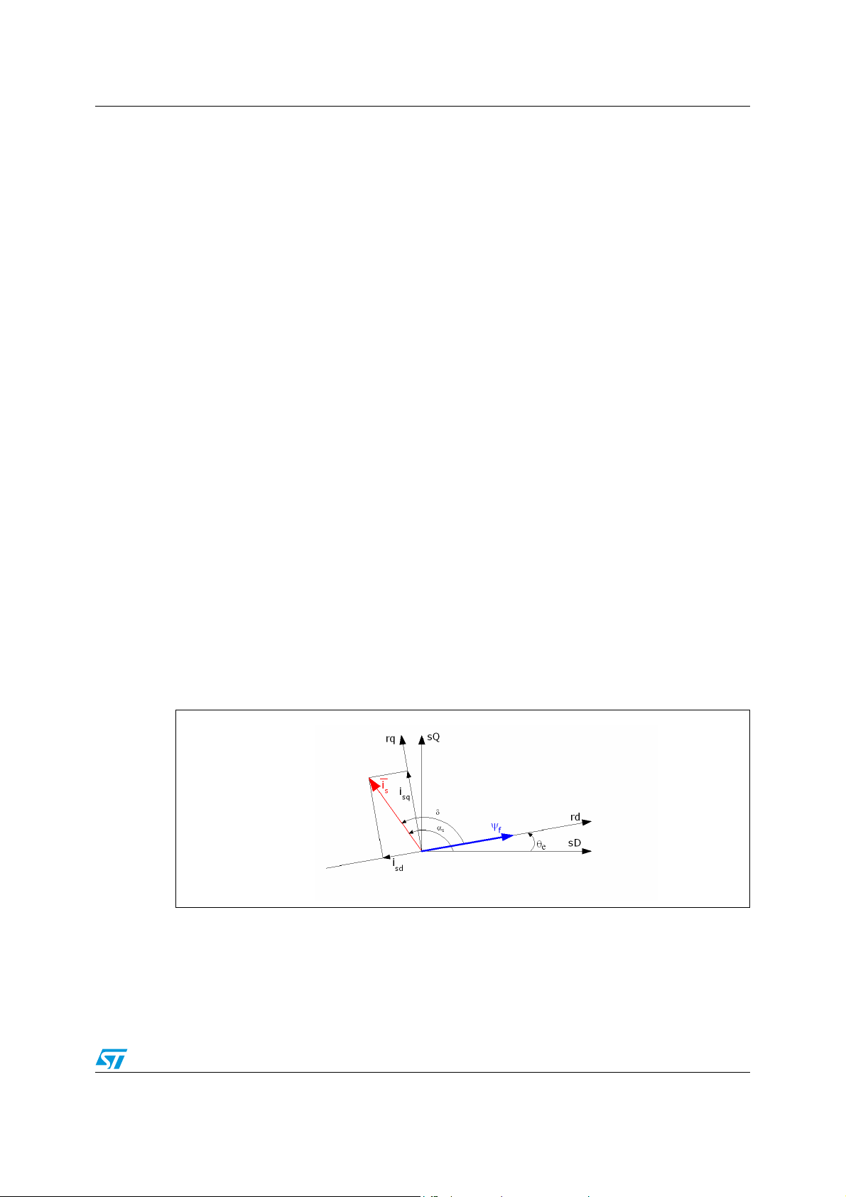
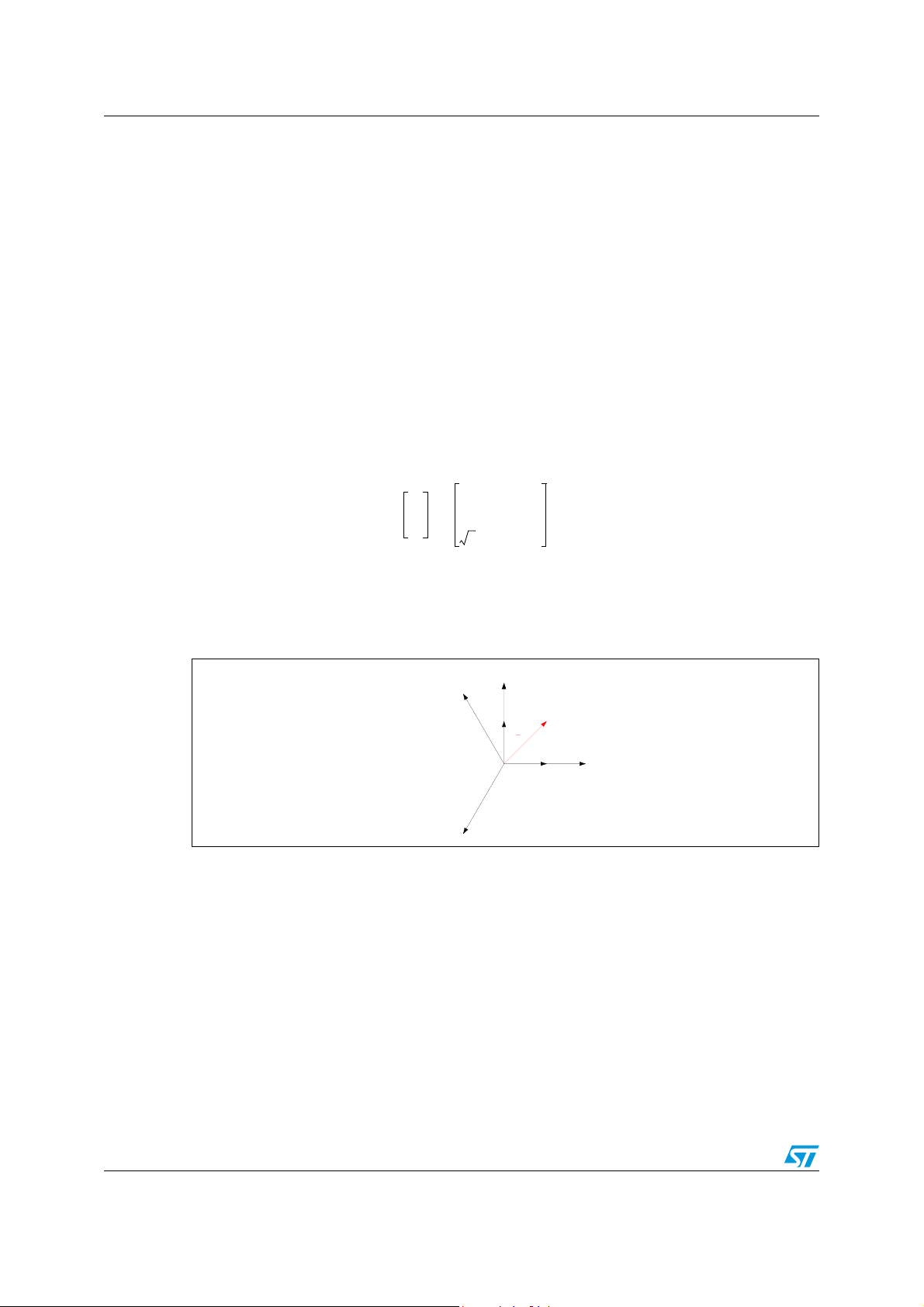
In the Figure 1, the Vector Diagram is shown:
Figure 1. Vector diagram
From this figure it is possible to understand that the direct-axis stator current component i
sd
is the only component in able to modify the field flux, weakening it.
Supposing constant field flux (setting to zero i
, if field weakening is no used), a quick
sdref
torque response is obtained changing only the quadrature-axis stator current component,
i
, by means of a current-controlled PWM inverter, as shows the following equation (2.2):
sq
7/53
Page 8

FOC-flux oriented control AN2290
We can conclude saying the Flux Oriented Control, handling instantaneous electrical
quantities, is a very accurate control in every working operation, either in steady state and in
transient, achieving high dynamic performance in terms of response times and power
conversion.
In this application note, the FOC control is explained using a particular AC machine, called
Permanent Magnetic Synchronous Machine (PMSM).
A short description of this machine, its features and mathematical model, follow before to
explain in details the FOC implementation.
2.1 PMSM
The necessity of reducing the charge of the combustion engine and of eliminating the weight
due to the mechanical connections in several applications, like in automotive field, induces
to use more and more electric motors, that assure a wide range in speed and torque control
satisfying the load demand.
The DC machine fulfils these requirements but needs periodic maintenance.
The AC machine, like induction motor and brushless permanent magnet motor, hasn’t
brushes, and its rotor is more robust because there aren’t commutator and/or rings. That
means a very low maintenance, other than increases the power-to-weight ratio and
efficiency.
3
T
--- pψ
el
2
fis
αsθe–()sin⋅
3
--- pψ
2
fis
3
δ()sin⋅
--- pψ
2
[2.2] ⋅===
fisq
In particular, in the automotive field the Permanent Magnet Synchronous Machine (PMSM)
seems to be the best solution.
The brushless permanent magnet motors (PMSMs) have the same electromagnetic
structure of a synchronous machine, without the brushes. As shown in the cross-section in
the Figure 2, they have a wound stator, similar to an induction machine, and a permanent
magnet rotor that replaces a rotor fed with dc current, like a synchronous machine. Besides,
they need of an internal or external device for sensing of the rotor position, like Hall sensors,
encoder or resolver.
Figure 2. Cross-section of PMSM
In fact the PMSMs are not self-commuting motors and to produce useful torque, the currents
and the voltages applied to stator phases must be controlled as a function of rotor position.
8/53
Page 9
AN2290 FOC-flux oriented control
Therefore it is generally required to count the rotor position with a sensor so that the inverter
phases which feed it, acting at any time, are commuted depending on the rotor position.
That explains the necessity of a closed-loop speed/position feedback.
There are two kinds of brushless permanent magnet machines classifiable in account of the
shape of the BEMF (back-electromagnetic force):
● DC brushless machine having trapezoidal flux distribution and a trapezoidal BEMF fed
by quasi-square wave currents;
● AC brushless machine having approximately sinusoidal air-gap flux density and a
quasi-sinusoidal BEMF fed by sinusoidal stator currents.
Generally the DC brushless machines have a simpler control strategy than AC brushless
machines.
For trapezoidal flux distributions, to impose quasi-square wave currents on stator windings,
it is only needed a six position sensor, with a resolution of at least 60° electrical degrees.
On the contrary, for the sinusoidal current type, the angular position needs to be known with
a very accurate precision in order to control each of the three phases currents.
For both kinds, the high reliability of control makes this type of machine a powerful system
for electric vehicle application.
2.2 Mathematical model of the machine
In order to model the fields produced by the stator windings in terms of windings current,
“current space vectors” are used. The current space vector for a given winding has the
direction of the field produced by that winding and a magnitude proportional to the current
through the winding. This allows us to represent the total stator field as a current space
vector that is the vector sum of three space vector components, one for each of the stator
windings.
The three-phase voltage, currents and fluxes of AC motors can be analyzed in terms of
complex space vectors.
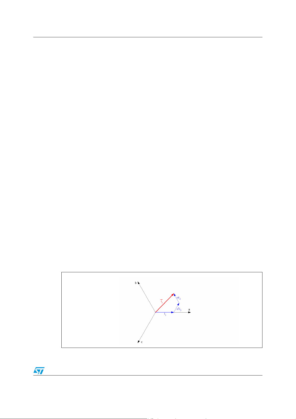
For instance, with regard to the currents in the stator windings, the current space vector can
be define as follows.
Figure 3. Stator current space vector and its components in (a,b,c)
9/53
Page 10

FOC-flux oriented control AN2290
Assuming that is1,is2,is3 are the instantaneous currents in the stator phases, then the
complex stator current vector i
is defined by:
s
2
where
α
= e
j(2π/3)
and
α
2
= e
i
s
--- i
s1is2
3
j(4π/3)
represent spatial operators. The Figure 3 shows the
α⋅ is3α2⋅++() [2.3]⋅=
stator current complex space vector.
That being stated, it is possible to write the mathematical model of an AC brushless
machine in a stator frame in terms of space vectors, as follows:
usRsisL
di
d
s
-------
dt
----- ψ
dt
s
jpθ
r
e
⋅() [2.4]+⋅+⋅=
f
where:
ψ
f
R
s
L
s
ω
r
p Number of pole pairs
θ
r
Modulus of the magnetizing flux-linkage vector
Stator resistance
Total three phase stator inductance
Rotor angular speed
Mechanical position
and the space vectors:
2π
-------
u
s
2
i
--- i
s
3
t() u2t() e
--- u
3
++
⎜⎟
1
⎝⎠
⎛⎞
t() i
⎜⎟
s1
⎝⎠
⎛⎞
2
⋅ u3t() e⋅
t() e
⋅ i
s
2
j
3
2π
j
-------
3
s
3
t() e
⋅++
4π
-------
j
3
Space vector of the stator voltage ⋅=
4π
j
-------
3
Space vector of the stator current⋅=
Note that the mechanical position of the electric motors is related to the rotation of the shaft
while the electrical position is relate to the rotation of the rotor magnetic field.
So being the motor with p pole pairs, its rotor needs only to move 360/p mechanical degrees
to obtain an identical magnetic configuration as when it started.
10/53
Page 11

AN2290 FOC-flux oriented control
Figure 4. Phase motor with 2 pole pair
Consequently the electric position of the rotor is linked to the mechanical position by the
relation:
θeθrp ⋅=
To complete the mathematical model of the motor, we include the equation of mechanical
equilibrium:
dω
r
J
--------- T
dt
+() [2.5]–=
eTmTν
and substituting the expression of the electric torque (2.2), it yields:
dω
---------
dt
1
r
--- T
eTmTν
J
+()–()⋅
1
3
⎛⎞
---
--- pψfi
⎝⎠
J
2
αsp θ⋅r–()TmTν+()–()sin⋅
s
[2.6]⋅==
where:
T
e
T
m
T
ν
α
s
J Inertia momentum of the machine
Electromagnetic torque
Mechanical torque
Viscose friction torque
Phase of the current space vector respect
Note: in Matlab-Simulink environment, the PMSM discrete model has been implemented
using a model of the machine in a stationary stator reference (D,Q) frame.
11/53
Page 12

FOC-flux oriented control AN2290
2.3 FOC control structure of PMSM
In Flux Oriented Control, motor currents and voltages are manipulated in the d-q reference
frame of the rotor. This means that measured motor currents must be mathematically
transformed from the three-phase stationary reference frame (a,b,c) of the stator windings to
the two axis rotating d-q reference frame, prior to processing, for example by PI controllers
(it is possible to use a different controller). Similarly, the voltages to be applied to the motor
are mathematically transformed from d-q frame of the rotor to the three phases reference
frame of stator before they can be used to produce the voltage control signals for the output
inverter that feeds the motor.
These transformations are the core of Flux Oriented Control.
Simplifying the expression of the electrical model of the machine, the projection from the
three-phase stationary reference frame of the stator windings to the two axis rotating
reference frame can be executed into two subsequent steps:
● (a,b,c) => (D,Q ) (the Clarke transformation) which outputs a two co-ordinate time
variant system;
● (D,Q ) => (d,q) (the Park transformation) which outputs a two co-ordinate time
invariant system;
where it is necessary to know in any time the current values in the stator phases and the
rotor position to execute the projections from a frame to other one, how explained in details
in the following.
Figure 5 is showing the block diagram of the FOC control library, where two motor phase
currents,(i.e. i
, is2), are measured with two current sensors (e.g. by phase shunts or
s1
current transducers) calculating the current in the third winding like the negative sum of the
other two windings, (i
= -(is1 + is2)), and then sending them to the Clarke transformation
s3
module, (Forward Clarke).
Outputs of this block are the two current components (i
, isQ) in the D,Q stator fixed frame.
sD
These components are used as inputs of the Park transformation module, (Forward Park),
that gives in output the current components (i
The i
reference) and i
and isq measured current components are compared to the references i
sd
(the torque reference) and corrected by mean of two PI controllers.
sqref
, isq) in the d,q rotating reference frame.
sd
sdref
(the flux
As in brushless synchronous permanent magnet motor the magnet flux is fixed (depending
on magnets), in the PMSM control, i
component in able to weak the flux, while the torque command i
the speed regulator, e.g. for a speed-FOC. That forces the current space vector i
exclusively in the quadrature direction, respect on the magnet flux vector. Since only i
should be set to zero, being the only current
sdref
could be the output of
sqref
to be
s
sq
produces useful torque, this maximizes the torque efficiency of the system.
Then the outputs of two PI, u
and usq, are sent to the Inverse Park transformation module,
sd
(Reverse Park), from which we get the new components of the stator voltage vector in the
(u
, usQ) non-rotating stator frame.
sD
12/53
Page 13
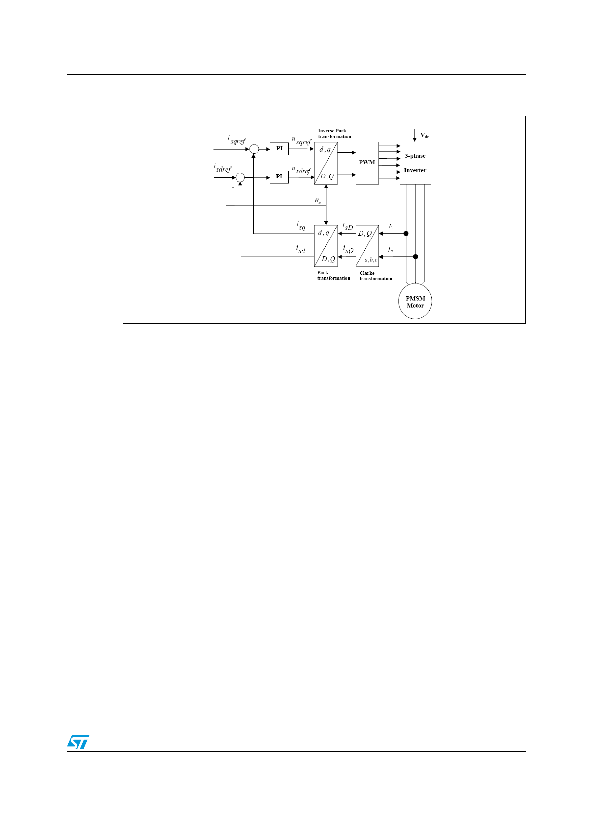
AN2290 FOC-flux oriented control
Figure 5. Block diagram of the flux oriented control library
These signals are then appropriately processed to produce voltage signals for the output
bridge.
In our case, it is chosen to use the Space Vector Modulation (SVM) technique to impress
the new voltage vector to the motor.
2.4 The space vector modulation theory
The SVM technique is a sophisticated continuous modulation method used, independently
from the type of implemented control on the motor, to generate a desired voltage space
vector at the output of the inverter that feeds the AC motor, in our case a PMSM. It uses a
special scheme to switch the power transistors generating pseudo-sinusoidal currents in the
stator windings.
This strategy offers the following advantages to the application:
● Higher performance to control mid/high dynamical motors;
● higher efficiency (86%);
● improved torque management;
● better start up performance;
● constant torque, less torque ripple;
● improved dynamical reaction.
To better understand the space vector modulation algorithm, it is before explained an other
fundamental component of the control system: the 3 phase inverter.
13/53
Page 14
FOC-flux oriented control AN2290
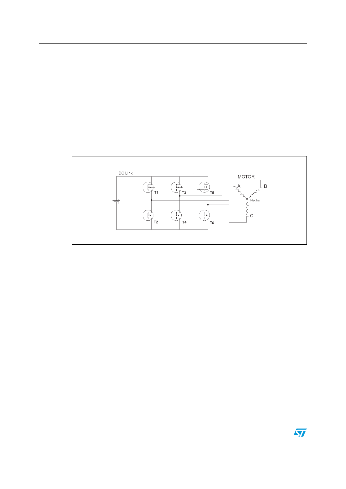
2.4.1 The 3-phase inverter
The inverter is a d.c. to a.c. converter. The Figure 6 shows the structure of a typical 3-phase
power inverter connected to the star motor windings, where V
The six switches can be power BJT, GTO, IGBT etc. The state-of-the-art solution for the
inverter power stages uses MOSFETs in low-voltage applications (i.e. automotive field).
The ON-OFF sequence of all these devices must respect the following conditions, so as to
feed in any time all three stator windings:
– three of the switches must always be ON and three always OFF.
– to avoid shortcut, the upper and lower switches of the same leg are driven with two
complementary pulsed signals
Figure 6. 3-phase power inverter scheme
is the DC Link voltage.
dc
On base of the aforementioned conditions, the inverter has only eight permissible switching
states of which six states apply a no-zero voltage to the motor windings and two states with
(V
and V7 ) zero volts when the motor is shorted through the upper or lower transistors.
0
It is useful to express the eight states of the inverter as space vectors: V
three voltages V
, VBn, VCn, that are spatially separated 120° apart, as a space vector for
An
expresses the
0-7
each of the switching states 0-7.
The six vectors including the zero voltage vectors can be expressed geometrically on the
complex plane as shown in the following Figure 7.
In order to generate a rotating field into the machine to produce a useful torque, the inverter
has to be switched in all the possible eight states. A way to use the inverter is the operating
mode called “six-step mode”, that generates high magnitude low order harmonics which
cannot be filtered by motor inductance.
14/53
Page 15
AN2290 FOC-flux oriented control
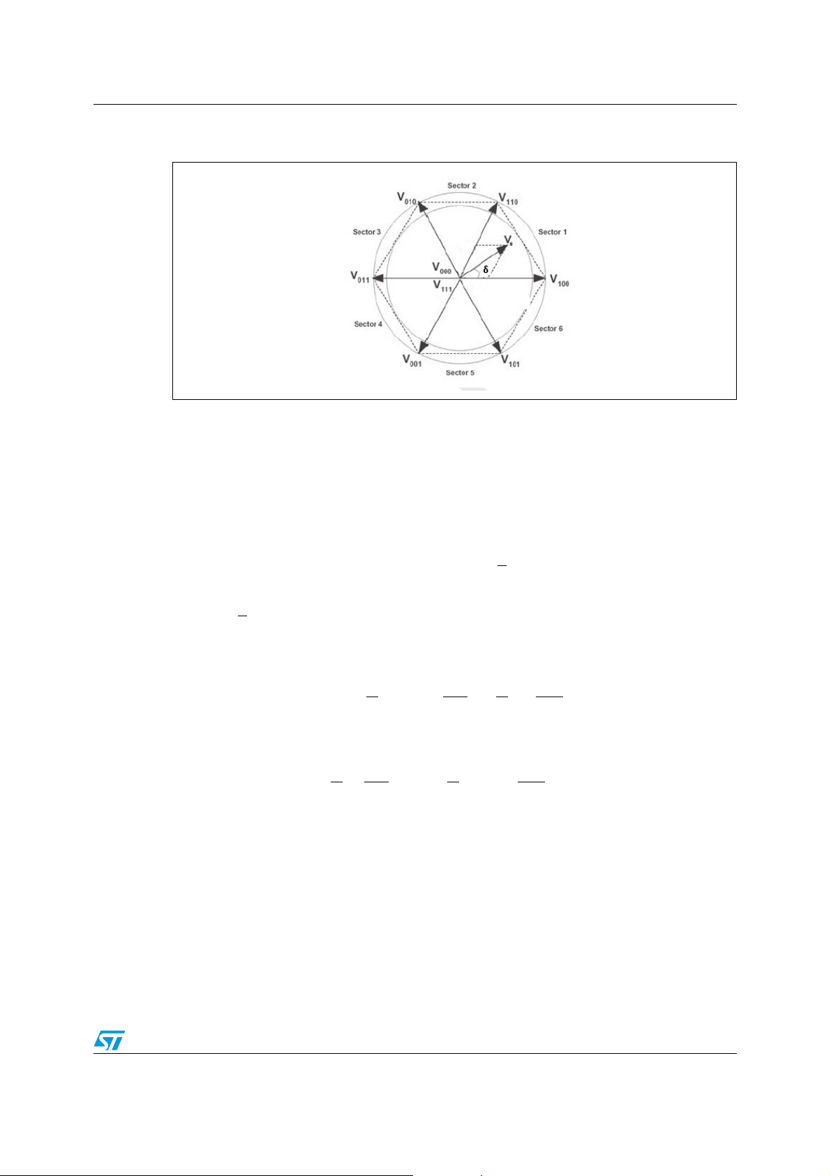
Figure 7. Space vector diagram
2.4.2 The Space vector pulse width modulation
The inverter is able to apply only eight space vector positions to the stator winding of an
electric machine, while the control imposes a voltage space vector that vary in all the inner
cycle of the hexagon in order to create a smooth rotating field (see Figure 7).
The SVM block, here implemented in Simulink, allows to generate the appropriate PWM
patter to impulse the inverter so that any voltage vector inside the space vector hexagon can
be produced by “time weighting“.
It is based on the fact that a reference voltage vector V
, can be realized by a combination of
s
the two adjacent active vectors and the zero vectors inside of sector where it lies. The output
space vector voltage (choosing an appropriate PWM period, T
the vector V
in this period), can be computed by the integral:
s
T
PWM
∫
0
Vstd⋅()
δ
⎛⎞
V
∫
⎝⎠
0
α
V
++
07⁄
∫
0
β
k
∫
0
V
k1+
so as to suppose steady
PWM,
[2.7]=
from which it yields:
VsV
07⁄
δ
---------------- V
T
PWM
α
---------------- V
k
T
PWM
k1+
----------------⋅+⋅+⋅=
T
PWM
β
where:
V
and V
k
included, T
V
0/V7
(k=0,..7) are the vectors that bound the sector in which the reference vector is
k+1
PWM
vectors in that sector.
T
PWM
is the switching period and α, β and δ are the time frames of Vk, V
αβδ [2.8]++=
and
k+1
15/53
Page 16
FOC-flux oriented control AN2290
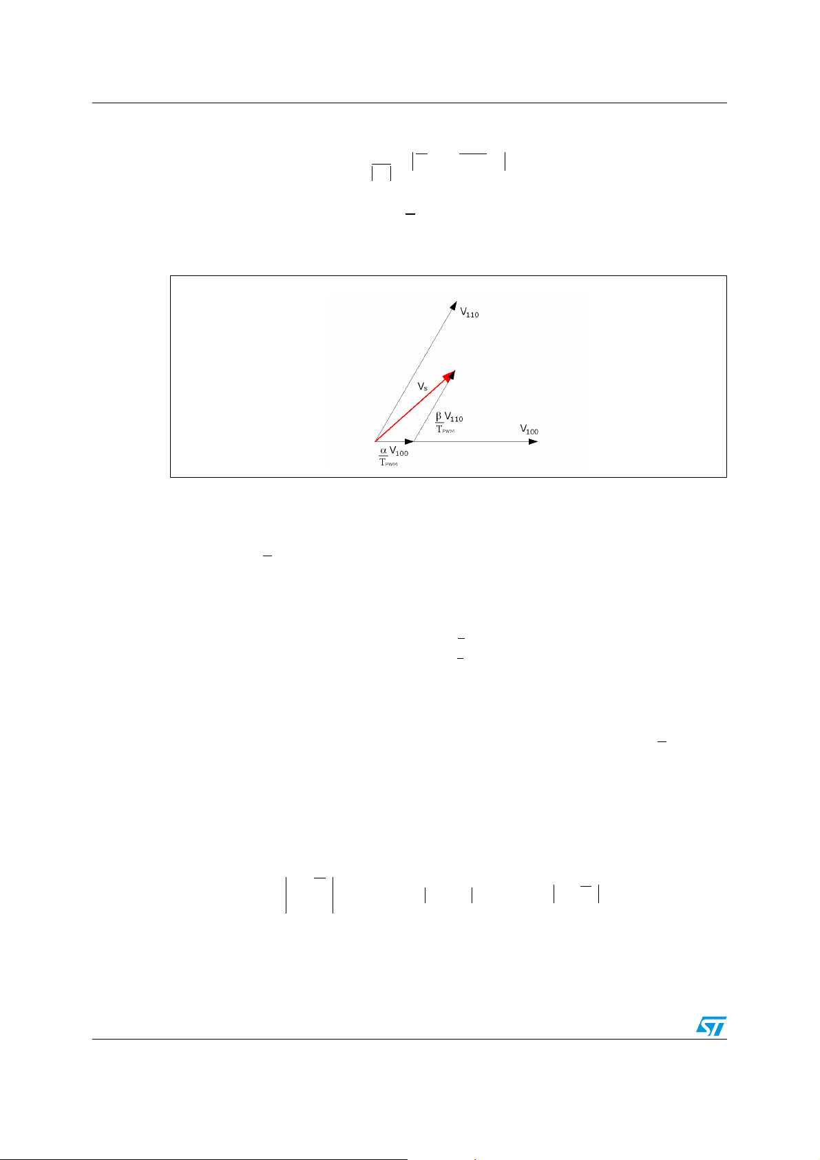
The resulting equation is:
For example, assuming that the vector V
Figure 8. SVM in the 1
in which α and β are the times during which the vectors V
2.4.3 Sector finder
st
sector
V
Vkα V
---------------------------------------------- [2.9] =
S
T
PWM
is in the 1st sector, we have the following situation:
s
k1+
β⋅+⋅
100
and V
are applied.
110
To impose the Vs voltage vector at the motor windings, it is fundamental the knowledge of
the sector where the reference vector is included for a correct behavior of SVM.
In the classic approach, in order to find the sector, you need to know the phase of the
complex reference vector that is calculated with the known formula:
⎛⎞
γ arc
ℑmVs()
---------------------
tan [2.10]=
⎜⎟
ℜeV
()
⎝⎠
s
The main problem of this formula is the calculation of arctan implemented on a 16bit
microcontroller. One solution can be to calculate the arctan making a look-up table of the
arctan function.
Another solution (here chosen) is to recognize the sector of reference vector V
, starting
s
from the knowledge of the sign of the imaginary (quadrature component) and real (direct
component) parts of the reference vector (u
sDref
, u
) written in a stator non-rotating
sQref
frame and the comparison of the their magnitudes in order to avoid the division in the
equation [2.10].If the vector phase obtained from the formula [2.11] is bigger than π/3 the
vector lies in sector 2 or 5. The control on sign of the components discriminates between the
sector 1-4 and 6-3 if the angle is less than π/3.
ℑmVs()
---------------------
()
ℜeV
s
arc
π
⎛⎞
---
tan≥ℑmV
⎝⎠
3
()arc
π
⎛⎞
---
s
tan ℜeV
⎝⎠
3
() [2.11]⋅≥⇒
s
iFigure 9 shows the exploded Sector Finder block:
16/53
Page 17

AN2290 FOC-flux oriented control
Figure 9. Sector finder schematic
2.4.4 SVM formulation
To create reference vector Vs inside one of the six sectors, the reference vectors which
bound that sector, have to be “time weighted”, like shown in the equation [2.9]. It is possible
to modulate the reference voltage vector and to apply the better switching pattern in term of
power dissipation on the power switches of the inverter and to make that, it is necessary to
choose the strategy to apply the vector V
We have some freedom degrees to choose the modulation algorithm as:
– The choice of the zero vector- whether V
– Sequencing of the vector;
– Splitting of the duty cycle of the vectors without introducing additional
commutations.
and V
k
(active vectors) in each sector.
k+1
(000) or V7(111) or both;
0
Literature demonstrates that, in order to reduce the number of commutation and switching
losses, it is preferable to utilize a states sequence where the states are adjacent.
This means that passing from a state to the successive one should occur with only one
switch commutation.
According to that, the scheme chosen is a symmetric sequence in which there are seven
conduction states, so called “Seven states Space Vector Modulation”.
Dividing the conduction time of every component of inverter in opportune time frames, as
shown below for a vector into Sector 1
:
Figure 10. Example of a switching pattern in sector 1
every component switches two times for every PWM period.
17/53
Page 18
FOC-flux oriented control AN2290
Analyzing the classical approach of SVM, it starts from the following equation:
VsT
⋅ Vkα V
PWM
k1+
β V0δ [2.12]⋅+⋅+⋅=
αβδ++ T
in which we are supposing steady in every period of PWM the vectors V
PWM
[2.13] =
, V
, V0 and Vs.
k
k+1
Projecting the vector equation [2.12] on the real and imaginary axis (D,Q) in the stator nonrotating frame, it yields:
α V
()Dβ V
k
α V
()Qβ V
k
()
⋅+⋅ usDT
k1+
D
()
⋅+⋅ usQT
k1+
Q
PWM
PWM
[2.14]⋅=
[2.15]⋅=
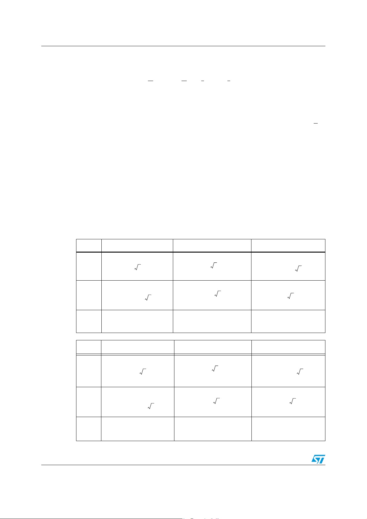
So solving the above said equations system for every sector, the following table will be
obtained:
Table 1. Time frames of application of V
Sector 1 Sector 2 Sector 3
α
----------------
T
PWM
u
---------
V
3
sD
⎛⎞
–
-------
⎝⎠
3
u
sQ
---------⋅
V
u
---------
V
sD
and V0
k,Vk+1
u
3
sQ
⎛⎞
---------⋅
+
-------
⎝⎠
V
3
u
---------
V
sD
2
--- 3⋅⋅
3
β
----------------
T
PWM
δ
T
u
---------
sQ
V
PWM
2
--- 3⋅⋅
3
α– β–
Sector 4 Sector 5 Sector 6
α
---------------- u
T
PWM
β
----------------
T
PWM
⎛⎞
⎝⎠
δ
---------–
sD
V
T
u
sQ
---------–
V
PWM
+
u
3
sQ
⎛⎞
---------⋅
-------
⎝⎠
V
3
2
--- 3⋅⋅
3
α– β–
18/53
u
sD
⎛⎞
⎝⎠
u
⎛⎞
---------
⎝⎠
⎛⎞
---------–
+
⎝⎠
V
T
PWM
u
sD
⎛⎞
---------–
–
-------
⎝⎠
V
sD
⎛⎞
–
⎝⎠
V
T
PWM
u
3
sQ
---------⋅
-------
V
3
α– β– T
u
3
sQ
---------⋅
V
3
u
3
sQ
---------⋅
-------
V
3
α– β– T
u
sD
⎛⎞
---------–
-------
–
⎝⎠
V
3
PWM
u
2
sD
---------–
--- 3⋅⋅
V
3
u
sD
⎛⎞
⎝⎠
⎛⎞
---------
+
-------
⎝⎠
V
PWM
3
α– β–
3
3
α– β–
u
sQ
---------⋅
V
u
sQ
---------⋅
V
Page 19

AN2290 FOC-flux oriented control
where V is .
2
⋅
--- V
3
dc
In this SVM algorithm, there isn’t the need of calculation of trigonometric functions to obtain
the time frames (α,β,δ), as it happens in a classical approach, and for every PWM period
only multiplications and divisions are needed.
The time frames so calculated from this algorithm must be processed with a look up table in
order to establish on which phase must be applied.
In the following table there are the time calculations to be done:
Sector 1 Sector 2 Sector 3 Sector 4 Sector 5 Sector 6
δ
α
---
2
T
PWM
----------------
2
---
4
δ
---+
4
δ
---–
4
t1
t2
t3
β
---
2
δ
---
4
T
PWM
----------------
2
δ
---+
4
T
PWM
----------------
2
δ
---
4
α
δ
---–
4
δ
---
---+
2
4
T
δ
----------------
---–
4
PWM
2
β
---
2
δ
---–
4
δ
---+
4
δ
---
4
α
---
2
T
PWM
----------------
2
δ
---+
4
δ
---–
4
δ
---
4
T
PWM
----------------
2
β
---
2
δ
---
4
δ
---–
4
δ
---+
4
19/53
Page 20
Flux control simulink library AN2290
3 Flux control simulink library
3.1 Description
The implementation of the FOC control needs of some peculiar functions. The Simulink
library implements all needed functions to built a FOC based electric motor control
application using the following blocks, here listed:
● Forward Clarke;
● Forward Park;
● Reverse Park;
● Sin_cos;
● PI;
● SVM.
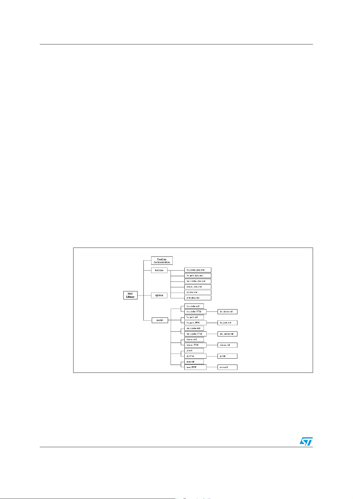
3.2 Using the simulink library
The 2 main directories of the library package are:
● 1 directory for all test cases: 1 subdirectory per library function;
● 1 directory for all .mdl files.
The file structure is the following:
Figure 11. Simulink library structure
3.2.1 How to install simulink library
The Simulink Library is delivered as an archive file with .zip extension. To install one you
need to unzip the file in the (C:) directory for a correct use.
20/53
Page 21

AN2290 Flux control simulink library
Note: you must have a 7.0.0 Matlab version or upward installed on your system to use this
library, plus a licence for Fixed-Point-Precision Toolbox to use the “convert block“in each
scheme block and a licence of RTW Embedded Coder Toolbox.
Please, read the README.txt file in the archive file for using the library.
3.2.2 Test environment
.mat: the inputs and outputs data obtained by Simulink in the double format are stored.
When the mdl file is opened data is loaded in Workspace of Matlab.
The name of each test-file begins with the (yyy) function name that it refers, followed by
underscore and the suffix “data”.
3.3 Parameters format
The FOC control system in Simulink has the same behavior of one implemented on micro
where it was necessary to use a different fixed point precision number representation in
every block. In the Tab le 2 the variables and their representations are listed:
Table 2. Data representation
variable representation description
i
s1
i
s2
i
s3
i
sD
i
sQ
sfix(16,8) phase current
sfix(16,8) phase current
sfix(16,8) phase current
sfix(16,8) direct-axis current component in stator fixed frame
sfix(16,8) quadrature-axis current component in stator fixed frame
theta_el ufix(16,16) electrical angle
cos_t sfix(16,14) cos(θe)
sin_t sfix(16,14) sin(θ
i
sd
i
sq
u
sd
u
sq
u
sQ
t
1
t
2
t
3
sfix(16,8) direct-axis current component in rotor no-fixed frame
sfix(16,8) quadrature-axis current component in rotor no-fixed frame
sfix(16,6) direct-axis voltage component in rotor no-fixed frame
sfix(16,6) quadrature-axis voltage component in rotor no-fixed frame
sfix(16,6) quadrature-axis voltage component in stator fixed frame
int16 time frames
int16 time frames
int16 time frames
)
e
In the following, the Simulink implemented blocks are described in details.
21/53
Page 22
Flux control simulink library AN2290
3.4 Clarke transformation
Description
The Clarke Transformation projects the motor currents (is1,is2,is3) from the 120° degrees
physical frame to a two co-ordinate stator non-rotating frame (i
Arguments
D,iQ
).
i
s1
i
s2
i
s3
i
sD
i
sQ
phase current;
phase current;
phase current;
direct-axis current component in stator fixed frame;
quadrature-axis current component in stator fixed frame.
Algorithm
The following equations are implemented:
i
i
sD
i
sQ
where assuming that the axis a (axis of the first phase) and the axis sD (stands for stator
direct axis) are in the same direction, we have the following vector diagram:
Figure 12. Stator current space vector
1
------- i
3
b
s1
–()⋅
s2is3
sQ
i
sQ
i
[3.1]=
s
a = sD
i
sD
We have so obtained a two co-ordinate system that still depends on time and speed.
Simulink block
As shown here below in the Figure 13, the Forward Clark block, implemented in Simulink,
receives in input the three current signals, here represented in sfix(16,8) fixed-point format,
returning in output the two current components, (i
same fixed-point format.
22/53
c
), in the stator fixed frame, in the
sD,isQ
Page 23

AN2290 Flux control simulink library
Figure 13. Forward Clarke block
Test case
In fw_clarke_data.mat file the inputs and outputs data to test this function are stored.
23/53
Page 24

Flux control simulink library AN2290
3.5 Park transformation
Description
The currents (isD,isQ) in the stator fixed frame are projected in the (d,q) rotor rotating frame
where the flux vector direction is chosen as the direct-axis d.
Arguments
i
sD
i
sQ
sin(θ
cos(θ
i
sd
i
sq
direct-axis current component in stator fixed frame;
quadrature-axis current component in stator fixed frame;
);
e
);
e
direct-axis current component in rotor no-fixed frame;
quadrature-axis current component in rotor no-fixed frame.
Algorithm
The following equations are implemented:
i
sd
i
sq
where (p
[3.2] the expressions of (i
θ
=
θ
) represents the electric position of the rotor flux. Substituting in the equation
r
e
sD,isQ
i
sd
i
sq
), it yields:
pθe()cos pθr()sin
()sin– pθe()cos
pθ
pθe()cos pθe()sin
()sin– pθe()cos
pθ
e
e
1
------- i
3
i
sD
i
sQ
i
s1
s2is3
[3.2]⋅=
[3.3]⋅=
–()⋅
here represented in the Figure 14:
Figure 14. Stator space vector into rotor frame
24/53
Page 25
AN2290 Flux control simulink library
Simulink block
As shown in the following, the Forward Park block, implemented in Simulink, receives in
input the two current components (i
returning in output the two current components (i
), here represented in sfix(16,8) fixed-point format,
sD,isQ
) in the rotor rotating frame, in the
sd,isq
same format.
Figure 15. Forward Park block
Test case
In fw_park_data.mat file the inputs and outputs data to test this function are stored.
25/53
Page 26

Flux control simulink library AN2290
3.6 Inverse Park transformation
Description
With this transformation, the voltage vectors outputs of PI controllers are projected from
rotor rotating frame in the stator fixed frame.
Arguments
u
sd
u
sq
sin(θ
cos(θ
u
sD
u
sQ
direct-axis voltage component in rotor no-fixed frame;
quadrature-axis voltage component in rotor no-fixed frame.
);
e
);
e
direct-axis voltage component in stator fixed frame;
quadrature-axis voltage component in stator fixed frame;
Algorithm
The following equations are implemented:
u
sD
u
sQ
pθr()cos pθr()sin–
()sin pθr()cos
pθ
r
u
sd
[3.4]⋅=
u
sq
Simulink block
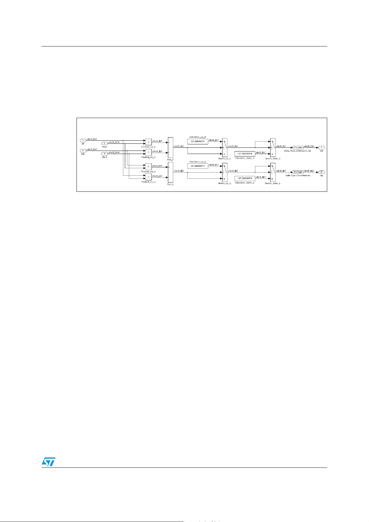
As shown here below in the Figure 16, the Reverse Park block, implemented in Simulink,
receives in input the two voltage components (u
point format, returning in output the two current components (u
frame, in the same format.
Figure 16. Reverse Park block
), here represented in sfix(16,6) fixed-
sd,usq
) in the rotor rotating
sD,usQ
Test case
In rev_clarke_data.mat file the inputs and outputs data to test this function are stored.
26/53
Page 27

AN2290 Flux control simulink library
3.7 Sin_cos
Description
Known the electrical position of the rotor, the functions sin(
project the space vectors from a frame to other one.
Arguments
θ
e
sin(θ
cos(θ
electrical position;
);
e
).
e
Algorithm
Simulink block
Figure 17. Sin_cos block
θ
) and cos(
e
θ
) are calculated to
e
Test case
In sincos_data.mat file the inputs and outputs data to test this function are stored.
27/53
Page 28

Flux control simulink library AN2290
3.8 PI block
Description
An electrical driver based on the FOC control needs of some controllers. In our case two PI
controllers: one for the torque component reference i
reference i
sdref
.
Arguments
i
(o i
sdref
i
(o isq) measured signal
sd
u
(o usq) command signal
sd
) reference signal
sqref
Algorithm
k1–
UkKpekKie
+⋅+⋅=
k
∑
n0=
Simulink block
The structure of the PI controller, in the discrete format, used in the Simulink model is shown
in Figure 18:
, one for the flux component
sqref
en [3.6]
Figure 18. PI structure
Test case
In pi_d_q_data.mat file the inputs and outputs data to test this function are stored.
The configuration parameters of PI are in pi_d_q_conf.mat file.
28/53
Page 29

AN2290 Flux control simulink library
3.9 SVM
Description
The goal of Space Vector Modulation is to generate three appropriate PWM signals to pulse
the inverter, that feeds the motor, so that three voltage vectors shifted (by 120° between
each other) can be produced on the phases of the motor.
Given a voltage space vector of module V
and angle γ, the implemented algorithm
s
modulates this vector in output applying on the inverter a switching pattern in order to
reduce the power dissipation on the electronic switches.
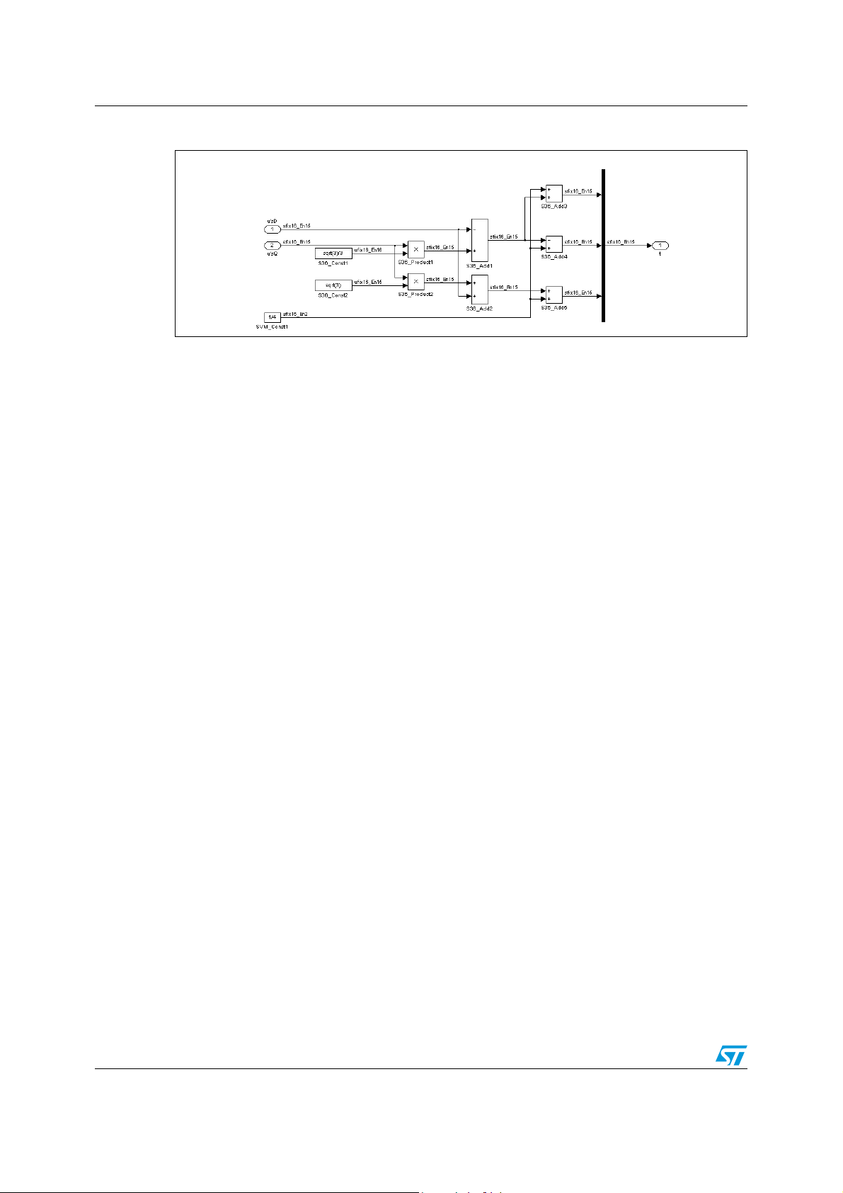
Figure 19. SVM scheme
It was possible to develop a Simulink block based on an optimized SVM algorithm, that
receives the outputs of the two PI controllers and the voltage of the DC link of the Inverter, to
produce the control signals.
How it is possible to view in the Figure 19, to implement the time frames of Tab le 1 ,we use
only three blocks for six sectors so to generate the appropriate switching pattern, choosing
on base of the actual sector where the vector V
lies in. This simplification, from six to three
s
blocks, it is possible observing that the six sectors are symmetric.
In this way we can calculate the time frames (t
) for each pair of sectors (1-4, 2-5 and
1 ,t2,t3
3-6) and with a Selector, from Sector Finder block, choose the right time frames.
Moreover the algorithm implements the dc-ripple-compensation by recalculating the voltage
components (u
sD ,usQ
) into relative voltages compared to measured dc-bus voltage:
U
′
U
s
-----------=
s
U
DC
where:
U
s
’
U
s
U
DC
is absolute voltage
is relative voltage
is dc-link voltage
29/53
Page 30

Flux control simulink library AN2290
Arguments
u
sD
u
sQ
V
DC
R
PWM
t
1 ,t2,t3
direct-axis voltage component in stator fixed frame;
quadrature-axis voltage component in stator fixed frame;
battery (or DC link) Voltage;
PWM resolution;
time frames.
Algorithm
We can calculate the time frames for each pair of sectors (1-4, 2-5 and 3-6) and with a
Selector, from Sector Finder block, choose the right time frames.
For instance, substituting the values of the time frames, α, β, δ, supposing a reference vector
in the Sector 1:
α T
β T
δ T
PWM
PWM
PWM
⋅⋅ ⋅=
⋅⋅ ⋅ ⋅=
substituting in the expressions of t
2
⎛⎞
--- u
⎝⎠
3
2
--- 3u
3
α– β–=
1,t2,t3
3
–
------- u⋅
sD
3
sQ
, it yields:
3
⎛⎞
---------⋅
---
⎝⎠
2
sQ
3
⎛⎞
---------⋅
---
⎝⎠
2
V
V
1
dc
1
dc
δ
t
--- T
1
4
α
t
2
t
3
δ
---
---+ T
2
4
T
PWM
----------------
2
1
′
⎛⎞
–
⋅==
--- u
PWM
⎝⎠
4
1
⎛⎞
--- u
PWM
⎝⎠
4
δ
---– T
PWM
4
3
′
⎛⎞
------- u
⋅
–
sD
′
sD
1
⎛⎞
--- u
⎝⎠
4
sQ
⎝⎠
3
′
3u
⋅–+
[3.7] ⋅==
sQ
′
3
′
⋅++
------- u
sD
sQ
3
⋅==
In the Sector 4 the result is the same, changing only the sign of the reference voltage vector
(u’
,u’sQ).
sD
Simulink block
In the following figure, the schema of the SVM is described:
30/53
Page 31

AN2290 Flux control simulink library
Figure 20. SVM implementation block
Here below it are exploded the blocks calculating in Simulink the time frames for a reference
vector inside the sector 1-4, 2-5 and 3-6.
Figure 21. Sector 1-4 implementation
Figure 22. Sector 2-5 implementation
31/53
Page 32
Flux control simulink library AN2290
Figure 23. Sector 6-3 implementation
The results of the SVM block are in int16 format.
Test Case
In svm_data.mat file the inputs and outputs data to test this function are stored.
32/53
Page 33
AN2290 Flux control software library
4 Flux control software library
4.1 Description
The Flux Control Software library provides the functions for mixed “C” and Assembly
programmers on ST10 microcontrollers necessary to implement an (FOC) electric motor
control.
4.2 Using the software library
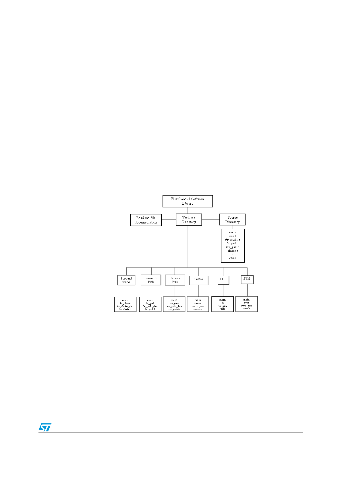
The 2 main directories of the library package are:
● 1 directory for all test cases: 1 subdirectory per library function.
● 1 directory for all .c sources file: all functions
The file structure is the following:
Figure 24. File structure
4.2.1 How to install Software library
The Software Library is delivered as an archive file with .zip extension. To install the
Software Library you need to unzip the file in the directory where you want the library to be
copied into.
Note: Please, read the README.txt file in the archive file for specific details on the release.
4.2.2 Tool chain compatibility
FOC library is compatible with Tasking tool chain (V7.5r2 and upward).
33/53
Page 34

Flux control software library AN2290
4.2.3 Calling a function
The functions have been written to be called by a C language program.
To include a function in a C language program, it is needed to:
● include the “emc.h”
● You find this .h file in the Source directory of the library package.
4.2.4 ST10 MAC configuration
This library has been done for implementing electric motor control functions (FOC control),
using 16-bit data in fixed point precision with different representations (i.e. sfix(16,8),
sfix(16,6), etc.). The implemented functions have been optimized with MAC commands
using the default configuration (the user have not to change the configuration registers of
MAC).
4.2.5 Real time aspects
Any DSP code developed for ST10 can be interrupted at any time and execution resumed
after the interrupt routine. There is no added latency when the DSP library is used.
Interrupt routine requirements: the only requirements are only when the DSP unit is used
by other tasks that have different priorities: the interrupting task that may interrupt another
task using the DSP should save and restore the MAC registers at the entry point and exit
point of the routine. (use #pragma savemac in Tasking tool chain).
4.2.6 Naming convention
The name of each functions coincides with the name of the Simulink equivalent block, that
implements it on micro.
Example: fw_park
The fw label represents the direction of the projection, from a (D,Q) frame to a (d,q) frame.
rev_park
The rev label represents the direction of the projection, from a (d,q) frame to a (D,Q) frame.
4.2.7 Test environment
yyy_data.c : you find the input data vectors and the output data vectors, obtained by
Simulink for the same function block, in int16 format.
The name of each test-file begins with the (yyy) function name that it refers, followed by
underscore and the suffix “data”.
4.2.8 Flux control library benchmark
The following table gives the characteristics of the main functions of the library:
34/53
Page 35

AN2290 Flux control software library
Table 3. FOC library capabilities
Function Code size (bytes) Nb cycles
Forward Clark 70 21
PID 226 57
Reverse park 538 48
SVM 822 74
SINCOS 532 56
35/53
Page 36

Flux control software library AN2290
4.3 Library functions
4.3.1 Forward Clarke
FCLARKE_c_step
FCLARKE_c_step(ExternalInputs_fw_clarke *fw_clarke_U, ExternalOutputs_fw_clarke
*fw_clarke_Y);
Data types and structures:
ExternalInputs_fw_clarke
This structure contains the motor phases currents.
typedef struct _ExternalInputs_fw_clarke_tag {
int16_T is1; phase current;
int16_T is2 phase current;
int16_T is3; phase current;
} ExternalInputs_fw_clarke;
ExternalOutputs_fw_clarke
This structure contains the current components in a fixed (D,Q) stator frame.
typedef struct _ExternalOutputs_fw_clarke_tag {
int16_T isD; current component in a fixed (D,Q) stator frame;
int16_T isQ; current component in a fixed (D,Q) stator frame;
} ExternalOutputs_fw_clarke;
Description:
It projects the motor currents (is1,is2,is3) from the 120° degrees physical frame to a two
co-ordinate stator non-rotanting frame (i
), using 16-bit operands.
D,iQ
Arguments:
fw_clarke_U pointer to the inputs structure
fw_clarke_Y pointer to the outputs structure
Algorithm:
isD
isQ
1
------- is2 is3–()⋅=
3
1
⎛⎞
------- is2 is3–()⋅
=
⎝⎠
3
Notes:
36/53
Page 37

AN2290 Flux control software library
Test:
To test this function, include the fw_clarke_data.c file in the current directory.
In the .c file you find the inputs and outputs vectors defined as const.
37/53
Page 38

Flux control software library AN2290
4.3.2 Forward Park
fw_park
FPARK_c_step(ExternalInputs_fw_park *fw_park_U, ExternalOutputs_fw_park
*fw_park_Y);
Description:
It projects the current components (isD,isQ) from the fixed stator frame in the (d,q) rotor
rotanting frame, using 16-bit operands.
Data types and structures:
ExternalInputs_fw_park
This structure contains the current components and the sin() and cos() functions of the
eletrical angle.
typedef struct _ExternalInputs_fw_park_tag {
int16_T isD; direct-axis current component in (D,Q) stator frame;
int16_T isQ; quadrature-axis current component in (D,Q) stator frame;
int16_T cos_t; cos(θ
int16_T sin_t; sin(θ
} ExternalInputs_fw_park;
)
e
)
e
ExternalOutputs_fw_park
This structure contains the current components in a no-fixed rotor frame.
typedef struct _ExternalOutputs_fw_park_tag {
int16_T isd; current component in a no-fixed rotor frame
int16_T isq; current component in a no-fixed rotor frame
} ExternalOutputs_fw_park;
Arguments:
fw_park_U pointer to the inputs structure
fw_park_Y pointer to the outputs structure
Algorithm:
isdi
sD
i
sqi–sD
θe()cos× i
θe()sin× i
sQ
sQ
θe()sin×+=
θe()cos×+=
Notes:
38/53
Page 39

AN2290 Flux control software library
Test:
To test this function, include the fw_park_data.c file in the current directory.
In the .c file you find the inputs and outputs vectors defined as const.
39/53
Page 40

Flux control software library AN2290
4.3.3 Reverse Park
rev_park
RPARK_c_step(ExternalInputs_rev_park *rev_park_U, ExternalOutputs_rev_park
*rev_park_Y);
Description:
It projects the outputs of PI controllers (usd,usq), from rotor rotating frame in the stator fixed
frame (u
Data types and structures:
ExternalInputs_rev_park
This structure contains the direct-axis and quadrature-axis voltage components in a no-fixed
(d,q) rotor frame and the sin() and cos() functions of the electrical angle.
typedef struct _ExternalInputs_rev_park_tag {
int16_T usd; direct-axis voltage component in a no-fixed (d,q) rotor frame
int16_T usq; quadrature-axis voltage component in a no-fixed (d,q) rotor frame
int16_T cos_t; cos(θ
int16_T sin_t; sin(θ
} ExternalInputs_rev_park;
), using 16-bit operands.
sD,usQ
)
e
)
e
ExternalOutputs_rev_park
This structure contains the current components in a (D,Q) stator frame.
typedef struct _ExternalOutputs_rev_park_tag {
int16_T usD;
direct-axis voltage component in (D,Q) stator frame
int16_T usQ; quadrature-axis voltage component in (D,Q) stator frame
} ExternalOutputs_rev_park;
Arguments:
rev_park_U pointer to the inputs structure
rev_park_Y pointer to the outputs structure
Algorithm:
usDu
u
sqQusd
sd
θe()cos× u
θe()sin× u
sq
sq
θe()sin×–=
θe()cos×+=
Notes:
40/53
Page 41

AN2290 Flux control software library
Test:
To test this function, include the rev_park_data.c file in the current directory.
In the .c file you find the inputs and outputs vectors defined as const.
41/53
Page 42

Flux control software library AN2290
4.3.4 Sin_Cos
sincos
SINCOS_c_step(ExternalInputs_sin_cos *sin_cos_U, ExternalOutputs_sin_cos
*sin_cos_Y);
Description:
Data types and structures:
ExternalInputs_sin_cos
This structure contains the current electrical angle.
typedef struct _ExternalInputs_sin_cos_tag {
uint16_T theta_el; θ
} ExternalInputs_sin_cos;
ExternalOutputs_sin_cos
This structure contains the sin() and cos() functions of the electrical angle.
typedef struct _ExternalOutputs_sin_cos_tag {
int16_T sin_t;; sin(θ
int16_T cos_t; cos(θ
} ExternalOutputs_sin_cos;
electrical position
e
)
e
)
e
Arguments:
sin_cos_U pointer to the inputs structure
sin_cos_Y pointer to the outputs structure
Algorithm:
Notes:
Test:
To test this function, include the sincos_data.c file in the current directory.
In the .c file you find the inputs and outputs vectors defined as const.
42/53
Page 43

AN2290 Flux control software library
4.3.5 PI controller
pi
pi_d_c_step(D_Work_pi_d *pi_d_DWork, ExternalInputs_pi_d *pi_d_U,
ExternalOutputs_pi_d *pi_d_Y);
pi_q_c_step(D_Work_pi_q *pi_q_DWork, ExternalInputs_pi_q *pi_q_U,
ExternalOutputs_pi_q *pi_q_Y);
Description:
It implements classical PI scheme for each control component (i
proportional and integral terms are forced to be in a range of values so as to calculate the
reference voltage signals,
(usd,usq), using 16-bit operands.
).The error and the
sd,isq
Data types and structures:
ExternalInputs_sin_cos
This structure contains the controlled signal (isd) of pi_d.
typedef struct _ExternalInputs_pi_d_tag {
int16_T isd;
} ExternalInputs_pi_d;
This structure contains the state of pi_d.
typedef struct D_Work_pi_d_tag {
int32_T state_d_DSTATE;
} D_Work_pi_d;
This structure contains the output signal (usd) of pi_d.
typedef struct _ExternalOutputs_pi_d_tag {
int16_T usd;
} ExternalOutputs_pi_d;
This structure contains the controlled signal (isq) of pi_q.
typedef struct _ExternalInputs_pi_q_tag {
int16_T isq;
} ExternalInputs_pi_q;
This structure contains the state of pi_q.
typedef struct D_Work_pi_q_tag {
int32_T state_q_DSTATE;
} D_Work_pi_q;
This structure contains the output signal (usq) of pi_q.
typedef struct _ExternalOutputs_pi_q_tag {
int16_T usq;
} ExternalOutputs_pi_q;
43/53
Page 44

Flux control software library AN2290
Arguments:
pi_d_DWork pointer to the state structure
pi_d_U pointer to the inputs structure
pi_d_U pointer to the outputs structure
Algorithm:
Notes:
Test:
To test this function, include the pi_data.c file in the current directory.
In the .c file you find the inputs and outputs vectors defined as const.
44/53
Page 45

AN2290 Flux control software library
4.3.6 SVM
svm
SVM_c_step(ExternalInputs_svm *svm_U, ExternalOutputs_svm *svm_Y);
Description:
It calculates three signals (t1,t2,t3 ) to impose the correct switching pattern on the Inverter,
using 16-bit operands.
Data types and structures:
ExternalInputs_svm
This structure contains (u
voltage,T
period of timer of PWM unit.
PWM
, usQ) the voltage components in (D,Q) stator frame, Vdc DC link
sD
typedef struct _ExternalInputs_svm_tag {
int16_T usD; direct-axis voltage component in (D,Q) stator frame
int16_T usQ; quadrature-axis voltage component in (D,Q) stator frame
uint16_T VBatt_meas; measured DC link voltage
uint16_T PWM_period; period of timer of PWM unit
} ExternalInputs_svm;
ExternalOutputs_svm
This structure contains the duty- cycles.
typedef struct _ExternalOutputs_svm_tag {
int16_T t1; duty cycle applied on first phase
int16_T t2; duty cycle applied on second phase
int16_T t3 duty cycle applied on third phase
} ExternalOutputs_svm;
Arguments:
svm_U pointer to the inputs structure
svm_Y pointer to the outputs structure
Algorithm:
The algorithm implements a different set of equations according to the actual position
of voltage vector, represented by its components (u
For example if the reference vector is in the Sector1:
1
t1T
t2T
′
⎛⎞
–
⋅=
--- u
PWM
⎝⎠
4
1
⎛⎞
PWM
--- u
⎝⎠
4
–
sD
′
sD
′
3
⎛⎞
⋅
------- u
sQ
⎝⎠
3
′
3u
⋅–+
⋅=
sQ
sD,usQ
).
45/53
Page 46

Flux control software library AN2290
1
′
3
t3T
⎛⎞
--- u
PWM
sD
⎝⎠
4
⋅++
------- u
3
′
sQ
⋅=
Notes:
Test:
To test this function, include the svm_data.c file in the current directory.
In the .c file you find the inputs and outputs vectors defined as const.
46/53
Page 47

AN2290 C code auto generation
5 C code auto generation
5.1 Overview
When the Simulink schematics are done, converted to fixed point precision and tested, the
last step is to generate C code downloadable on the microcontroller. This step is done using
two toolboxes of Matlab:
● The Real Time Workshop
● The Real Time Workshop Embedded Coder
The Real Time Workshop is an essential tool used in rapid prototyping with Simulink.
Automatic program building allows you to make design changes directly to the block
diagram, putting algorithm development (including coding, compiling, linking, and
downloading to target hardware) under control of a single process.
In this part, a set of signal processing functions for C programmers on ST10 are presented.
5.2 Steps to generate optimized C code
● Design a model in Simulink
The rapid prototyping process begins with the development of a model in Simulink. Using
principles of control engineering, it’s possible to model plant dynamics and other dynamic
components that constitute a controller and/or an observer.
● Simulate the Model in Simulink
Using MATLAB-Simulink, and toolboxes it’s possible to develop algorithms and analyze the
results.If the results are not satisfactory, it’s possible to iterate the modelling and analysis
process until results are acceptable.
● Generate Source Code with Real-Time Workshop
Once simulation results are acceptable, it’s possible to generate downloadable C code that
implements the appropriate portions of the model. Simulink could be used in external mode
to monitor signals, tune parameters, and further validate and refine the model, quickly
iterating through solutions.
● Implement a Production Prototype
At this stage, the rapid prototyping process is complete.
5.3 Real-Time Workshop
The Real-Time Workshop Embedded Coder is a separate, add-on product for use with
Real-Time Workshop.
It is intended for use in embedded systems development to generate code that is easy to
read, trace, and customize for all production environment. The Real-Time Workshop
Embedded Coder provides a framework for the development of production code that is
optimized for speed, memory usage, and simplicity. It generates optimized ANSI-C or ISO-C
code for fixed point and floating point microprocessors. It extends the capabilities provided
by the Real-Time Workshop to support specification, integration, deployment, and testing of
production applications on embedded targets. The Real Time Workshop Embedded Coder
47/53
Page 48

C code auto generation AN2290
addresses targeting considerations such as RAM, ROM, and CPU constraints, code
configuration, and code verification.
The Embedded Real-Time (ERT) target, provided by the Real Time Workshop Embedded
Coder, is designed for customization.
Figure 25. Flow chart
In our applications we use the ERT target with optimization for fixed point systems. Correct
specification of target-specific characteristics of generated code (such as word sizes for
char, int, and long data types, or desiderated rounding behaviors in integer operations) can
be critical in embedded systems development. The Hardware Implementation category of
options in the settings menu provides a simple and flexible way to control such
characteristics in both simulation and code generation.
5.4 How to generate C code using Real Time Workshop
Starting from a model in fixed point precision it is described step by step how to generate C
code.
For the example, the inner loop of FOC control will be considered and starting from the
Simulink schematic the C code will be automatically generate.
48/53
Page 49
AN2290 C code auto generation
Step 1 - Simulink schematic constructor
The first step is the construction of the Simulink schematic implementing the considered
function.
Note: for improving the readability of the auto generated C-code it’s useful to include the
schematic of each single function in a single subsystem.
In Figure 26, it’s possible to see also the signal format. The model is now ready to be
compiled in order to generate C code.
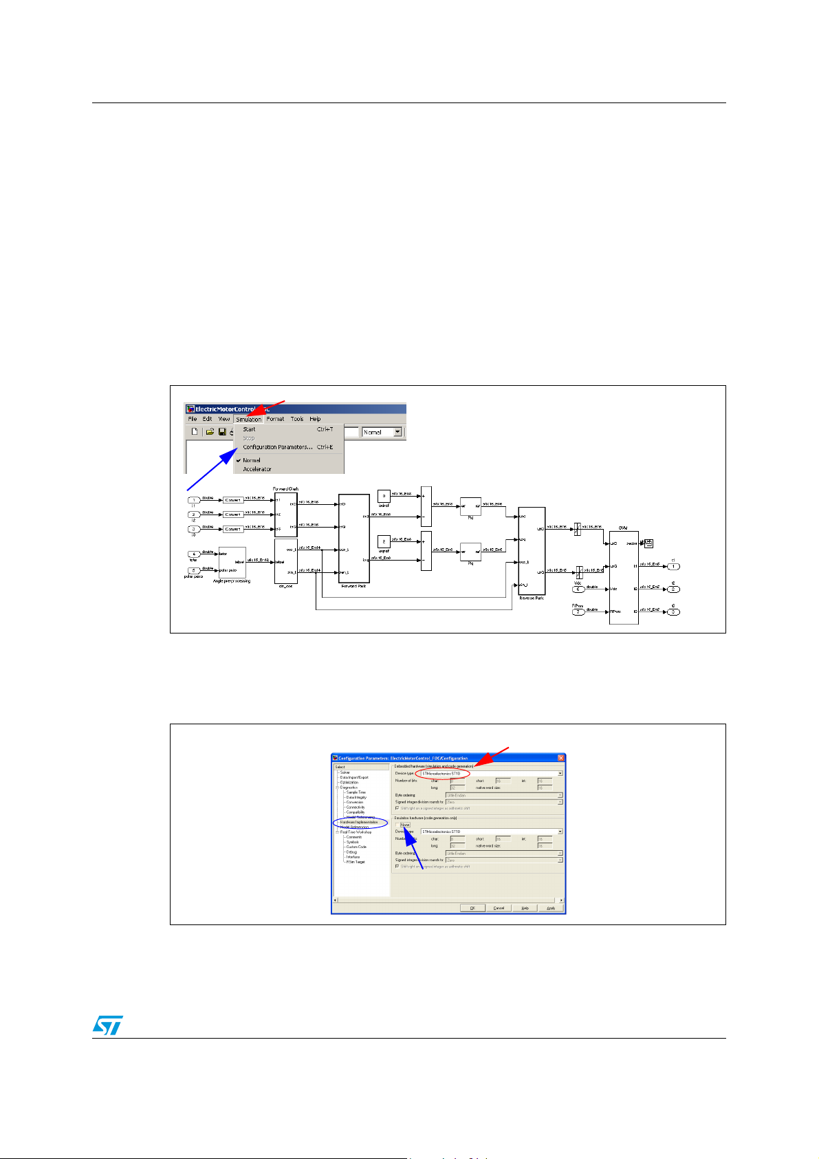
Step 2 - Real Time Workshop options configuration
Selecting from the Simulation menu the “Configuration Parameter” pane all the options are
shown:
Figure 26. Configuration parameter
The first thing to do is selecting the Hardware Implementation, in our case ST10. In this way
the format of data are chosen.
Figure 27. Hardware implementation
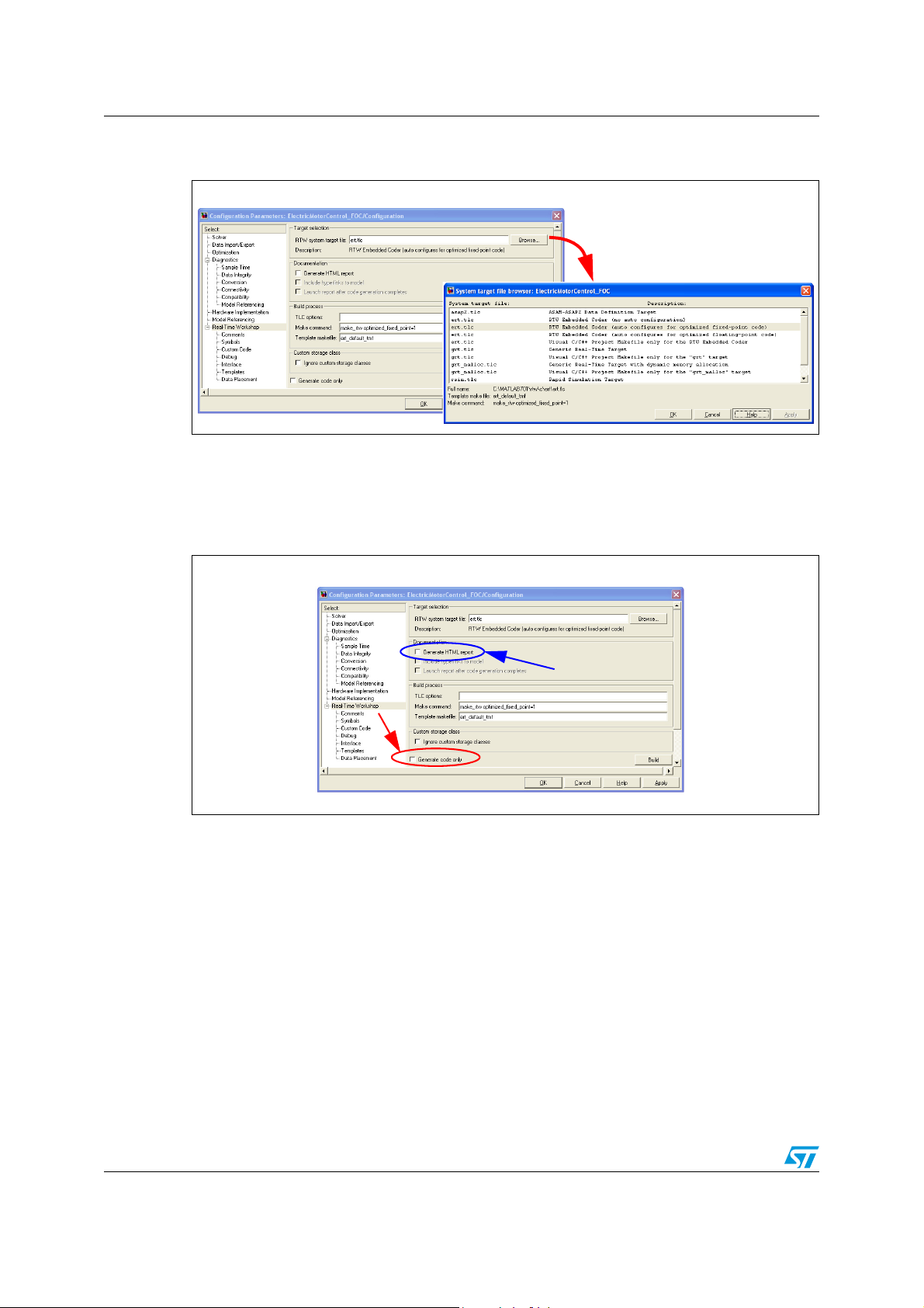
After the Real time Workshop options must be chosen. The first one is the RTW system
target. As before said we choose the ERT optimum for fixed point precision (Figure 28).
49/53
Page 50
C code auto generation AN2290
Figure 28. RTW system target file
a) b)
If only the code is needed (as in our case), the Generate code only box must be checked,
(Figure 29), furthermore you could auto generate the Generate HTML report checking the
apposite box.
Figure 29. Generate HTML
In the Comments pane it’s possible to define the verbosity level of the compiler and the
comments that are automatically included in the generated C code.
Now everything is ready for generating code. Pushing the “Generate code“ button the code
generation starts with some verbose comments in the Matlab command windows,
(Figure 30).
50/53
Page 51

AN2290 C code auto generation
Figure 30. Generate code
a) b)
When the process is completed the HTML report windows will appear generating the files:
● ElectricMotorControl_FOC.c
● ElectricMotorControl_FOC.h
● rtwtypes.h
Not all of them are useful for the next step code download.
5.5 Automatic configuration of RTW
Running RTWconfiguration.m file in the Command Window of Matlab available in the folder
C:\FOC_Library2.0\options, a set of parameters is loaded to configure the RTW and
associated with a given filename.mdl. For Automatic configuration the following steps has to
be followed:
● Open filename.mdl file;
● Copy RTWconfiguration.m and config_RTW.mat in the actual working directory;
● Run “RTWconfiguration” from Command Window of Matlab.
In this way you’ll get active the “RTW_configuration” set to run and auto generate the C
code.
51/53
Page 52

Revision history AN2290
6 Revision history
Table 4. Document revision history
Date Revision Changes
9-Mar-2007 1 Initial release.
52/53
Page 53

AN2290
Please Read Carefully:
Information in this document is provided solely in connection with ST products. STMicroelectronics NV and its subsidiaries (“ST”) reserve the
right to make changes, corrections, modifications or improvements, to this document, and the products and services described herein at any
time, without notice.
All ST products are sold pursuant to ST’s terms and conditions of sale.
Purchasers are solely responsible for the choice, selection and use of the ST products and services described herein, and ST assumes no
liability whatsoever relating to the choice, selection or use of the ST products and services described herein.
No license, express or implied, by estoppel or otherwise, to any intellectual property rights is granted under this document. If any part of this
document refers to any third party products or services it shall not be deemed a license grant by ST for the use of such third party products
or services, or any intellectual property contained therein or considered as a warranty covering the use in any manner whatsoever of such
third party products or services or any intellectual property contained therein.
UNLESS OTHERWISE SET FORTH IN ST’S TERMS AND CONDITIONS OF SALE ST DISCLAIMS ANY EXPRESS OR IMPLIED
WARRANTY WITH RESPECT TO THE USE AND/OR SALE OF ST PRODUCTS INCLUDING WITHOUT LIMITATION IMPLIED
WARRANTIES OF MERCHANTABILITY, FITNESS FOR A PARTICULAR PURPOSE (AND THEIR EQUIVALENTS UNDER THE LAWS
OF ANY JURISDICTION), OR INFRINGEMENT OF ANY PATENT, COPYRIGHT OR OTHER INTELLECTUAL PROPERTY RIGHT.
UNLESS EXPRESSLY APPROVED IN WRITING BY AN AUTHORIZED ST REPRESENTATIVE, ST PRODUCTS ARE NOT
RECOMMENDED, AUTHORIZED OR WARRANTED FOR USE IN MILITARY, AIR CRAFT, SPACE, LIFE SAVING, OR LIFE SUSTAINING
APPLICATIONS, NOR IN PRODUCTS OR SYSTEMS WHERE FAILURE OR MALFUNCTION MAY RESULT IN PERSONAL INJURY,
DEATH, OR SEVERE PROPERTY OR ENVIRONMENTAL DAMAGE. ST PRODUCTS WHICH ARE NOT SPECIFIED AS "AUTOMOTIVE
GRADE" MAY ONLY BE USED IN AUTOMOTIVE APPLICATIONS AT USER’S OWN RISK.
Resale of ST products with provisions different from the statements and/or technical features set forth in this document shall immediately void
any warranty granted by ST for the ST product or service described herein and shall not create or extend in any manner whatsoever, any
liability of ST.
ST and the ST logo are trademarks or registered trademarks of ST in various countries.
Information in this document supersedes and replaces all information previously supplied.
The ST logo is a registered trademark of STMicroelectronics. All other names are the property of their respective owners.
© 2007 STMicroelectronics - All rights reserved
STMicroelectronics group of companies
Australia - Belgium - Brazil - Canada - China - Czech Republic - Finland - France - Germany - Hong Kong - India - Israel - Italy - Japan -
Malaysia - Malta - Morocco - Singapore - Spain - Sweden - Switzerland - United Kingdom - United States of America
www.st.com
53/53
 Loading...