Siemens SIMATIC NET PROFIBUS User Manual

Download

Symbols, Contents

SIMATIC NET PROFIBUS Networks

Manual

PROFIBUS Networks Topologies of SIMATIC NET PROFIBUS

Networks Configuring Networks

Passive Components of RS–485 Networks

Active Components of RS–485 Networks

Passive Components for PROFIBUS–PA

Passive Components for Electrical Networks

Active Components for Optical Networks

Active Components for Wireless Networks

1 2 3 4 5 6 7 8 9

Testing PROFIBUS Lightning and Surge Voltage Protection for

LAN Cables Between Buildings Installing LAN Cables

Installing Instructions for SIAMTIC NET PROFIBUS Plastic Fiber Optic with Simplex Connenctors or BFOC Connectors and Pulling Loop for the FO Standard Cable

Installing Network Components in Cubicles

Dimension Drawings

Operating Instructions ILM / OLM / OBT

General Information

References

A B C

D E

F G H

05/2000 6GK1970–5CA20–0AA1 Release 2

SIMATIC NET – Support and Training Glossary, Index

Safety Guidelines

Danger

indicates that death, severe personal injury or substantial property damage will result if proper precau- tions are not taken.

Warning

indicates that death, severe personal injury or substantial property damage can result if proper precautions are not taken.

Caution

indicates that minor personal injury or property damage can result if proper precautions are not taken.

Note

draws your attention to particularly important information on the product, handling the product, or to a particular part of the documentation.

Qualified Personnel

Only qualified personnel should be allowed to install and work on this equipment Qualified persons are defined as persons who are authorized to commission, to ground, and to tag circuits, equipment, and systems in accordance with established safety practices and standards.

Correct Usage

Note the following:

Warning

Trademarks

The reproduction, transmission or use of this document or its contents is not permitted without express written authority. Offenders will be liable for damages. All rights, including rights created by patent grant or registration of a utility model or design, are reserved.

This device and its components may only be used for the applications described in the catalog or the technical description, and only in connection with devices or components from other manufacturers which have been approved or recommended by Siemens.

This product can only function correctly and safely if it is transported, stored, set up, and installed correctly, and operated and maintained as recommended.

SIMATICR, SIMATIC HMIR and SIMATIC NETR are registered trademarks of SIEMENS AG.

HCS is a registered trademark of Ensign–Bickford Optics Company.

Third parties using for their own purposes any other names in this document which refer to trademarks might infringe upon the rights of the trademark owners.

We have checked the contents of this manual for agreement with the hardware and software described. Since deviations cannot be precluded entirely, we cannot guarantee full agreement. However, the data in this manual are reviewed regularly and any necessary corrections included in subsequent editions. Suggestions for improvement are welcomed.

Siemens AG Bereich Automatisierungs– und Antriebstechnik Geschäftsgebiet Industrielle Kommunikation Postfach 4848, D-90327 Nürnberg

Siemens Aktiengesellschaft Order no. 6GK 1970–5AC20–0AA1

E Siemens AG 1999 Subject to technical change.

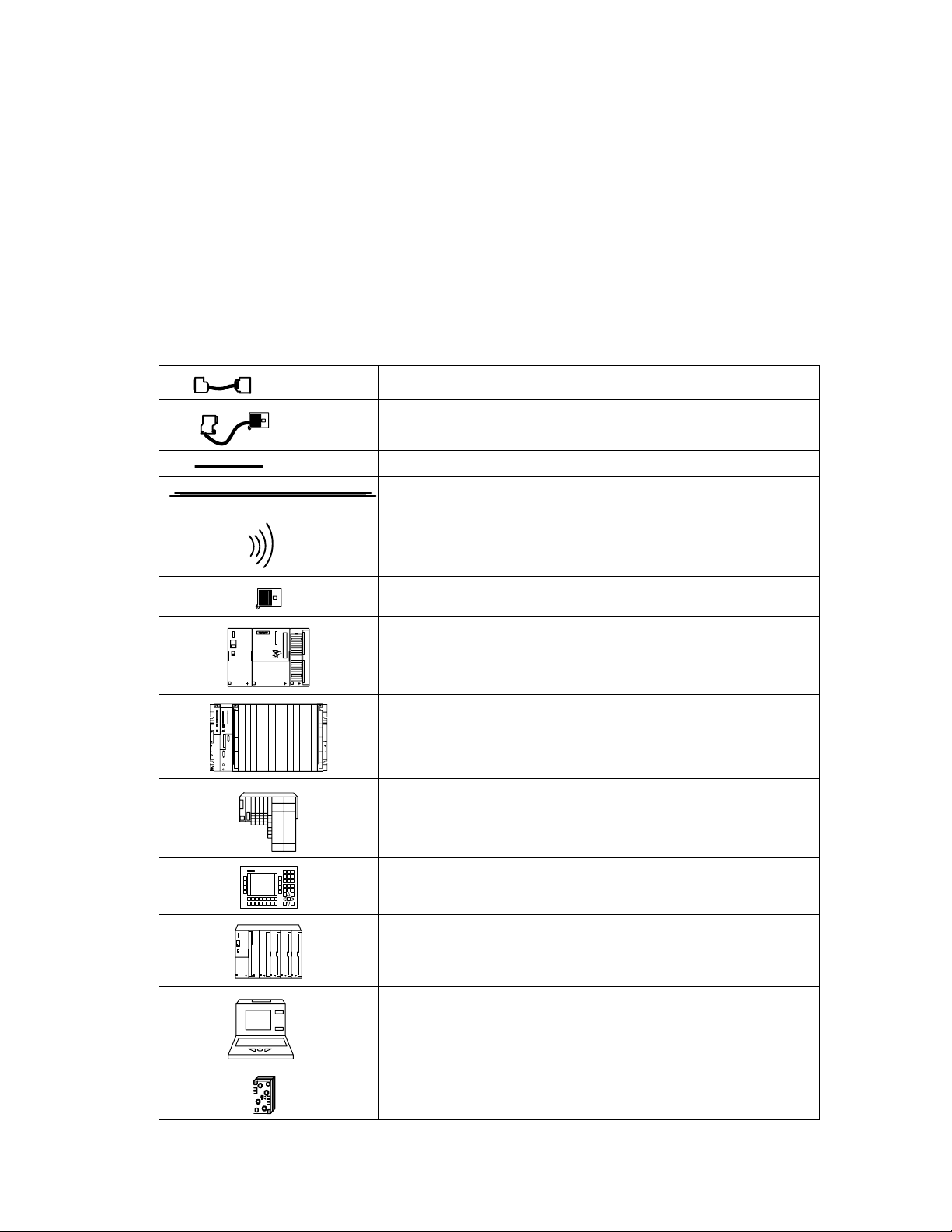
Symbols

PROFIBUS 830–1 T connecting cable PROFIBUS 830-2 connecting cable

LAN cable (twisted-pair) Duplex FO cable Wireless transmission (infrared)

Bus connector

S7–300

PROFIBUS Networks SIMATIC NET 6GK1970-5CA20-0AA1 Release 2 05/2000

S7–400

ET200S

OP25

ET 200M (with IM 153–2 FO)

PG/PC/OP

AS-i branch

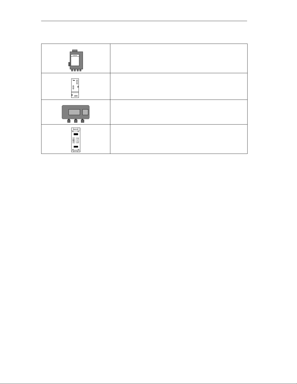
Symbols

Optical link module (OLM)

Optical bus terminal (OBT)

Infrared link module (ILM)

Repeater

PROFIBUS Networks SIMATIC NET

6GK1970-5CA20-0AA1 Release 2 05/2000

Contents

1 PROFIBUS NETWORKS 1-1. . . . . . . . . . . . . . . . . . . . . . . . . . . . . . . . . . . . . . . . . . . . . . . . .

1.1 Local Area Networks in Manufacturing and Process Automation 1-2. . . . . . .

1.1.1 General Introduction 1-2. . . . . . . . . . . . . . . . . . . . . . . . . . . . . . . . . . . . . . . . . . . . .

1.1.2 Overview of the SIMATIC NET System 1-3. . . . . . . . . . . . . . . . . . . . . . . . . . . . .

1.2 Basics of the PROFIBUS Network 1-5. . . . . . . . . . . . . . . . . . . . . . . . . . . . . . . . .

1.2.1 Standards 1-7. . . . . . . . . . . . . . . . . . . . . . . . . . . . . . . . . . . . . . . . . . . . . . . . . . . . . .

1.2.2 Access Techniques 1-8. . . . . . . . . . . . . . . . . . . . . . . . . . . . . . . . . . . . . . . . . . . . . .

1.2.3 Transmission Techniques 1-9. . . . . . . . . . . . . . . . . . . . . . . . . . . . . . . . . . . . . . . . .

1.2.4 Transmission Techniques According to EIA Standard RS-485 1-10. . . . . . . . .

1.2.5 Transmission Techniques for Optical Components 1-12. . . . . . . . . . . . . . . . . . .

1.2.6 Transmission Technique for Wireless Infrared Technology 1-14. . . . . . . . . . . . .

1.2.7 Transmission Technique for PROFIBUS-PA 1-15. . . . . . . . . . . . . . . . . . . . . . . . .

2 Topologies of SIMATIC NET PROFIBUS Networks 2-1. . . . . . . . . . . . . . . . . . . . . . . . .

2.1 Topologies of RS-485 Networks 2-2. . . . . . . . . . . . . . . . . . . . . . . . . . . . . . . . . . .

2.1.1 Components for Transmission Rates up to 1.5 Mbps 2-3. . . . . . . . . . . . . . . .

2.1.2 Components for Transmission Rates up to

12 Mbps 2-4. . . . . . . . . . . . . . . . . . . . . . . . . . . . . . . . . . . . . . . . . . . . . . . . . . . . . . .

2.2 Topologies of Optical Networks 2-5. . . . . . . . . . . . . . . . . . . . . . . . . . . . . . . . . . . .

2.2.1 Topology with Integrated Optical Interfaces 2-6. . . . . . . . . . . . . . . . . . . . . . . . .

2.2.2 Topologies with OLMs 2-7. . . . . . . . . . . . . . . . . . . . . . . . . . . . . . . . . . . . . . . . . . . .

2.2.3 Combination of Integrated Optical Interfaces and OLMs 2-13. . . . . . . . . . . . . .

2.3 Topologies of Wireless Networks 2-14. . . . . . . . . . . . . . . . . . . . . . . . . . . . . . . . . .

2.4 Topologies with PROFIBUS-PA 2-17. . . . . . . . . . . . . . . . . . . . . . . . . . . . . . . . . . .

2.5 Connectivity Devices 2-20. . . . . . . . . . . . . . . . . . . . . . . . . . . . . . . . . . . . . . . . . . . . .

2.5.1 DP/DP Coupler 2-20. . . . . . . . . . . . . . . . . . . . . . . . . . . . . . . . . . . . . . . . . . . . . . . . .

2.5.2 Connecting to PROFIBUS-PA 2-22. . . . . . . . . . . . . . . . . . . . . . . . . . . . . . . . . . . . .

2.5.3 DP/PA Coupler 2-23. . . . . . . . . . . . . . . . . . . . . . . . . . . . . . . . . . . . . . . . . . . . . . . . . .

2.5.4 DP/PA Link 2-25. . . . . . . . . . . . . . . . . . . . . . . . . . . . . . . . . . . . . . . . . . . . . . . . . . . . .

2.5.5 Connecting PROFIBUS-DP to RS-232C 2-28. . . . . . . . . . . . . . . . . . . . . . . . . . . .

2.5.6 Connecting with the DP/AS-Interface Link 65 2-30. . . . . . . . . . . . . . . . . . . . . . .

2.5.7 Connecting with the DP/AS-Interface Link 20 2-33. . . . . . . . . . . . . . . . . . . . . . . .

2.5.8 Connecting PROFIBUS-DP to instabus EIB 2-36. . . . . . . . . . . . . . . . . . . . . . . . .

3 Configuring Networks 3-1. . . . . . . . . . . . . . . . . . . . . . . . . . . . . . . . . . . . . . . . . . . . . . . . . .

3.1 Configuring Electrical Networks 3-2. . . . . . . . . . . . . . . . . . . . . . . . . . . . . . . . . . .

3.1.1 Segments for Transmission Rates up to a Maximum of 500 Kbps 3-3. . . . . .

3.1.2 Segments for a Transmission Rate of 1.5 Mbps 3-4. . . . . . . . . . . . . . . . . . . . .

3.1.3 Segments for Transmission Rates up to a Maximum of

12 Mbps 3-8. . . . . . . . . . . . . . . . . . . . . . . . . . . . . . . . . . . . . . . . . . . . . . . . . . . . . . .

3.1.4 Configuring Electrical Networks with RS-485 Repeaters 3-9. . . . . . . . . . . . . .

3.2 Configuring Optical Networks 3-11. . . . . . . . . . . . . . . . . . . . . . . . . . . . . . . . . . . . .

3.2.1 How a Fiber-Optic Cable Transmission System Works 3-12. . . . . . . . . . . . . . .

3.2.2 Optical Power Budget of a Fiber-Optic Transmission System 3-14. . . . . . . . . .

3.2.3 Cable Lengths for Plastic and PCF FO Paths 3-17. . . . . . . . . . . . . . . . . . . . . . .

3.2.4 Calculating the Power Budget of Glass Fiber Optical Links with OLMs 3-18. .

PROFIBUS Networks SIMATIC NET 6GK1970-5CA20-0AA1 Release 2 05/2000

iii

Contents

3.3 Transmission Delay Time 3-22. . . . . . . . . . . . . . . . . . . . . . . . . . . . . . . . . . . . . . . . .

3.3.1 Configuring Optical Buses and

Star Topologies with OLMs 3-23. . . . . . . . . . . . . . . . . . . . . . . . . . . . . . . . . . . . . . .

3.3.2 Configuring Redundant Optical Rings with OLMs 3-27. . . . . . . . . . . . . . . . . . . .

3.3.3 Example of Configuring the Bus Parameters in STEP 7 3-31. . . . . . . . . . . . . . .

4 Passive Components for RS-485 Networks 4-1. . . . . . . . . . . . . . . . . . . . . . . . . . . . . . .

4.1 SIMATIC NET PROFIBUS Cables 4-2. . . . . . . . . . . . . . . . . . . . . . . . . . . . . . . . .

4.1.1 FC Standard Cable 4-7. . . . . . . . . . . . . . . . . . . . . . . . . . . . . . . . . . . . . . . . . . . . . .

4.1.2 FC-FRNC Cable (LAN cable with halogen-free outer sheath) 4-8. . . . . . . . . .

4.1.3 FC Food Cable 4-9. . . . . . . . . . . . . . . . . . . . . . . . . . . . . . . . . . . . . . . . . . . . . . . . .

4.1.4 FC Robust Cable 4-10. . . . . . . . . . . . . . . . . . . . . . . . . . . . . . . . . . . . . . . . . . . . . . . .

4.1.5 PROFIBUS Flexible Cable 4-11. . . . . . . . . . . . . . . . . . . . . . . . . . . . . . . . . . . . . . . .

4.1.6 FC Underground Cable 4-13. . . . . . . . . . . . . . . . . . . . . . . . . . . . . . . . . . . . . . . . . .

4.1.7 FC Trailing Cable 4-14. . . . . . . . . . . . . . . . . . . . . . . . . . . . . . . . . . . . . . . . . . . . . . . .

4.1.8 PROFIBUS Festoon Cable 4-18. . . . . . . . . . . . . . . . . . . . . . . . . . . . . . . . . . . . . . .

4.1.9 SIENOPYR-FR Marine Cable 4-22. . . . . . . . . . . . . . . . . . . . . . . . . . . . . . . . . . . . .

4.2 FastConnect Bus Connector 4-24. . . . . . . . . . . . . . . . . . . . . . . . . . . . . . . . . . . . . .

4.2.1 The FastConnect System 4-24. . . . . . . . . . . . . . . . . . . . . . . . . . . . . . . . . . . . . . . .

4.2.2 Area of Application and Technical Specifications of the FastConnect Bus

Connector 4-25. . . . . . . . . . . . . . . . . . . . . . . . . . . . . . . . . . . . . . . . . . . . . . . . . . . . . .

4.2.3 Using the FastConnect Stripping Tool for Preparing FC Cables 4-30. . . . . . . .

4.3 Bus Connectors 4-32. . . . . . . . . . . . . . . . . . . . . . . . . . . . . . . . . . . . . . . . . . . . . . . . .

4.3.1 Area of Application and Technical Specifications of the Bus Connector 4-33. .

4.4 Attaching the LAN Cable to the Bus Connector 4-37. . . . . . . . . . . . . . . . . . . . . .

4.4.1 Attaching the LAN Cable to Bus Connector (6ES7 972-0B.11..) 4-37. . . . . . . .

4.4.2 Connecting the LAN Cable to Bus Connector (6ES7 972-0BA30-0XA0) 4-40.

4.4.3 Connecting the LAN Cable to Bus Connector (6ES7 972-0B.40) 4-42. . . . . . .

4.5 Installing the Bus Connector with Axial Cable Outlet 4-44. . . . . . . . . . . . . . . . . .

4.6 Plugging the Bus Connector into the Module 4-46. . . . . . . . . . . . . . . . . . . . . . . .

4.7 Bus Terminals for RS-485 Networks 4-48. . . . . . . . . . . . . . . . . . . . . . . . . . . . . . .

4.7.1 Versions 4-48. . . . . . . . . . . . . . . . . . . . . . . . . . . . . . . . . . . . . . . . . . . . . . . . . . . . . . .

4.7.2 Design and Functions of the RS-485 Bus Terminal 4-49. . . . . . . . . . . . . . . . . . .

4.7.3 Design and Functions of the 12M Bus Terminal 4-52. . . . . . . . . . . . . . . . . . . . . .

4.7.4 Mounting/Attaching the LAN Cables 4-55. . . . . . . . . . . . . . . . . . . . . . . . . . . . . . .

4.7.5 Grounding 4-58. . . . . . . . . . . . . . . . . . . . . . . . . . . . . . . . . . . . . . . . . . . . . . . . . . . . . .

4.7.6 Technical Data of the RS-485 Bus Terminal 4-60. . . . . . . . . . . . . . . . . . . . . . . . .

4.7.7 Technical Data of the 12M Bus Terminal 4-61. . . . . . . . . . . . . . . . . . . . . . . . . . . .

4.8 Cable Connections 4-63. . . . . . . . . . . . . . . . . . . . . . . . . . . . . . . . . . . . . . . . . . . . . .

4.8.1 Cable Connections to Network Components 4-63. . . . . . . . . . . . . . . . . . . . . . . .

4.8.2 Cable Connection without Bus Connection Elements 4-63. . . . . . . . . . . . . . . . .

4.9 Preassembled Connecting Cables 4-65. . . . . . . . . . . . . . . . . . . . . . . . . . . . . . . . .

4.9.1 830-1T Connecting Cable 4-65. . . . . . . . . . . . . . . . . . . . . . . . . . . . . . . . . . . . . . . .

4.9.2 830-2 Connecting Cable 4-67. . . . . . . . . . . . . . . . . . . . . . . . . . . . . . . . . . . . . . . . . .

5 Active Components for RS-485 Networks 5-1. . . . . . . . . . . . . . . . . . . . . . . . . . . . . . . . .

5.1 RS-485 Repeater 5-2. . . . . . . . . . . . . . . . . . . . . . . . . . . . . . . . . . . . . . . . . . . . . . . .

5.2 Possible Configurations with the RS-485 Repeater 5-6. . . . . . . . . . . . . . . . . . .

PROFIBUS Networks SIMATIC NET

6GK1970-5CA20-0AA1 Release 2 05/2000

Contents

5.3 Installing and Uninstalling the RS-485 Repeater 5-9. . . . . . . . . . . . . . . . . . . . .

5.4 Ungrounded Operation of the RS-485 Repeater 5-12. . . . . . . . . . . . . . . . . . . . .

5.5 Connecting the Power Supply 5-13. . . . . . . . . . . . . . . . . . . . . . . . . . . . . . . . . . . . .

5.6 Connecting the LAN Cable 5-14. . . . . . . . . . . . . . . . . . . . . . . . . . . . . . . . . . . . . . .

5.7 PROFIBUS Terminator 5-15. . . . . . . . . . . . . . . . . . . . . . . . . . . . . . . . . . . . . . . . . . .

6 Passive Components for PROFIBUS-PA 6-1. . . . . . . . . . . . . . . . . . . . . . . . . . . . . . . . . .

6.1 FC Process Cable 6-2. . . . . . . . . . . . . . . . . . . . . . . . . . . . . . . . . . . . . . . . . . . . . . .

6.2 SpliTConnect Tap 6-3. . . . . . . . . . . . . . . . . . . . . . . . . . . . . . . . . . . . . . . . . . . . . . .

7 Passive Components for Electrical Networks 7-1. . . . . . . . . . . . . . . . . . . . . . . . . . . . .

7.1 Fiber-Optic Cables 7-2. . . . . . . . . . . . . . . . . . . . . . . . . . . . . . . . . . . . . . . . . . . . . .

7.2 Plastic Fiber-Optic Cables 7-3. . . . . . . . . . . . . . . . . . . . . . . . . . . . . . . . . . . . . . . .

7.2.1 Plastic Fiber Optic, Duplex Cord 7-5. . . . . . . . . . . . . . . . . . . . . . . . . . . . . . . . . . .

7.2.2 Plastic Fiber-Optic, Standard Cables 7-7. . . . . . . . . . . . . . . . . . . . . . . . . . . . . . .

7.2.3 PCF Fiber-Optic Cables 7-10. . . . . . . . . . . . . . . . . . . . . . . . . . . . . . . . . . . . . . . . . .

7.3 Glass Fiber-Optic Cables 7-13. . . . . . . . . . . . . . . . . . . . . . . . . . . . . . . . . . . . . . . . .

7.3.1 Fiber-Optic Standard Cable 7-17. . . . . . . . . . . . . . . . . . . . . . . . . . . . . . . . . . . . . . .

7.3.2 INDOOR Fiber-Optic Cable 7-18. . . . . . . . . . . . . . . . . . . . . . . . . . . . . . . . . . . . . . .

7.3.3 Flexible Fiber-Optic Trailing Cable 7-19. . . . . . . . . . . . . . . . . . . . . . . . . . . . . . . . .

7.3.4 SIENOPYR Duplex Fiber-Optic Marine Cable 7-22. . . . . . . . . . . . . . . . . . . . . . .

7.3.5 Special Cables 7-24. . . . . . . . . . . . . . . . . . . . . . . . . . . . . . . . . . . . . . . . . . . . . . . . . .

7.4 Fiber-Optic Connectors 7-26. . . . . . . . . . . . . . . . . . . . . . . . . . . . . . . . . . . . . . . . . .

7.4.1 Connectors for Plastic Fiber-Optic Cables 7-26. . . . . . . . . . . . . . . . . . . . . . . . . .

7.4.2 Simplex Connector and Adapter for Devices with Integrated Optical Interfaces . 7-26

7.4.3 BFOC Connectors for OLMs 7-30. . . . . . . . . . . . . . . . . . . . . . . . . . . . . . . . . . . . . .

7.4.4 Connectors for Glass Fiber Cables 7-30. . . . . . . . . . . . . . . . . . . . . . . . . . . . . . . .

8 Active Components for Optical Networks 8-1. . . . . . . . . . . . . . . . . . . . . . . . . . . . . . . .

8.1 Optical Bus Terminal OBT 8-2. . . . . . . . . . . . . . . . . . . . . . . . . . . . . . . . . . . . . . . .

8.2 Optical Link Module OLM 8-4. . . . . . . . . . . . . . . . . . . . . . . . . . . . . . . . . . . . . . . . .

9 Active Components for Wireless Networks 9-1. . . . . . . . . . . . . . . . . . . . . . . . . . . . . . .

9.1 Infrared Link Module ILM 9-2. . . . . . . . . . . . . . . . . . . . . . . . . . . . . . . . . . . . . . . . .

A Testing PROFIBUS A-1. . . . . . . . . . . . . . . . . . . . . . . . . . . . . . . . . . . . . . . . . . . . . . . . . . . . .

A.1 Hardware Test Device BT200 for PROFIBUS-DP A-2. . . . . . . . . . . . . . . . . . . .

A.1.1 Possible Uses A-2. . . . . . . . . . . . . . . . . . . . . . . . . . . . . . . . . . . . . . . . . . . . . . . . . .

A.1.2 Area of Application A-2. . . . . . . . . . . . . . . . . . . . . . . . . . . . . . . . . . . . . . . . . . . . . .

A.1.3 Logging Functions A-2. . . . . . . . . . . . . . . . . . . . . . . . . . . . . . . . . . . . . . . . . . . . . . .

A.1.4 Design A-3. . . . . . . . . . . . . . . . . . . . . . . . . . . . . . . . . . . . . . . . . . . . . . . . . . . . . . . . .

A.1.5 Functions A-4. . . . . . . . . . . . . . . . . . . . . . . . . . . . . . . . . . . . . . . . . . . . . . . . . . . . . .

A.1.6 How the Unit Functions A-5. . . . . . . . . . . . . . . . . . . . . . . . . . . . . . . . . . . . . . . . . .

A.2 Testing FO Transmission Paths A-7. . . . . . . . . . . . . . . . . . . . . . . . . . . . . . . . . . .

A.2.1 Necessity of a Final Test A-7. . . . . . . . . . . . . . . . . . . . . . . . . . . . . . . . . . . . . . . . .

A.2.2 Optical Power Source and Meter A-7. . . . . . . . . . . . . . . . . . . . . . . . . . . . . . . . . .

A.2.3 Optical Time Domain Reflectometer (OTDR) A-9. . . . . . . . . . . . . . . . . . . . . . . .

PROFIBUS Networks SIMATIC NET 6GK1970-5CA20-0AA1 Release 2 05/2000

Contents

A.2.4 Checking the Optical Signal Quality with PROFIBUS OLM V3 A-12. . . . . . . . .

B Lightning and Surge Voltage Protection for LAN Cables Between Buildings B-1

B.1 Why Protect Your Automation System From Overvoltage? B-2. . . . . . . . . . . .

B.2 Protecting LAN Cables from Lightning B-2. . . . . . . . . . . . . . . . . . . . . . . . . . . . . .

B.2.1 Instructions for Installing Coarse Protection B-5. . . . . . . . . . . . . . . . . . . . . . . . .

B.2.2 Instructions for Installing Fine Protection B-6. . . . . . . . . . . . . . . . . . . . . . . . . . . .

B.2.3 General Information on the Lightning Protection Equipment from the Firm of

Dehn & Söhne B-7. . . . . . . . . . . . . . . . . . . . . . . . . . . . . . . . . . . . . . . . . . . . . . . . . .

C Installing LAN Cables C-1. . . . . . . . . . . . . . . . . . . . . . . . . . . . . . . . . . . . . . . . . . . . . . . . . . .

C.1 LAN Cables in Automation Systems C-2. . . . . . . . . . . . . . . . . . . . . . . . . . . . . . .

C.2 Electrical Safety C-3. . . . . . . . . . . . . . . . . . . . . . . . . . . . . . . . . . . . . . . . . . . . . . . . .

C.3 Mechanical Protection of LAN Cables C-4. . . . . . . . . . . . . . . . . . . . . . . . . . . . . .

C.4 Electromagnetic Compatibility of LAN Cables C-7. . . . . . . . . . . . . . . . . . . . . . .

C.4.1 Measures to Counter Interference Voltages C-7. . . . . . . . . . . . . . . . . . . . . . . . .

C.4.2 Installation and Grounding of Inactive Metal Parts C-8. . . . . . . . . . . . . . . . . . .

C.4.3 Using the Shields of Electrical LAN Cables C-8. . . . . . . . . . . . . . . . . . . . . . . . . .

C.4.4 Equipotential Bonding C-10. . . . . . . . . . . . . . . . . . . . . . . . . . . . . . . . . . . . . . . . . . . .

C.5 Routing Electrical LAN Cables C-13. . . . . . . . . . . . . . . . . . . . . . . . . . . . . . . . . . . .

C.5.1 Cable Categories and Clearances C-13. . . . . . . . . . . . . . . . . . . . . . . . . . . . . . . . .

C.5.2 Cabling within Closets C-16. . . . . . . . . . . . . . . . . . . . . . . . . . . . . . . . . . . . . . . . . . .

C.5.3 Cabling within Buildings C-16. . . . . . . . . . . . . . . . . . . . . . . . . . . . . . . . . . . . . . . . . .

C.5.4 Cabling outside Buildings C-17. . . . . . . . . . . . . . . . . . . . . . . . . . . . . . . . . . . . . . . . .

C.5.5 Special Noise Suppression Measures C-18. . . . . . . . . . . . . . . . . . . . . . . . . . . . . .

C.6 Electromagnetic Compatibility of Fiber-Optic Cables C-20. . . . . . . . . . . . . . . . .

C.7 Installing LAN Cables C-21. . . . . . . . . . . . . . . . . . . . . . . . . . . . . . . . . . . . . . . . . . . .

C.7.1 Instructions for Installing Electrical and Optical LAN cables C-21. . . . . . . . . . . .

C.8 Additional Instructions on Installing Fiber-Optic Cables C-24. . . . . . . . . . . . . . .

D Installation Instructions for SIMATIC NET PROFIBUS Plastic Fiber-Optic with

Simplex Connectors or BFOC Connectors and Pulling Loop for the FO Standard

Cable D-1. . . . . . . . . . . . . . . . . . . . . . . . . . . . . . . . . . . . . . . . . . . . . . . . . . . . . . . . . . . . . . . . . .

E Installing Network Components in Cubicles E-1. . . . . . . . . . . . . . . . . . . . . . . . . . . . . .

E.1 IP Degrees of Protection E-1. . . . . . . . . . . . . . . . . . . . . . . . . . . . . . . . . . . . . . . . .

E.2 SIMATIC NET Components E-3. . . . . . . . . . . . . . . . . . . . . . . . . . . . . . . . . . . . . . .

F Dimension Drawings F-1. . . . . . . . . . . . . . . . . . . . . . . . . . . . . . . . . . . . . . . . . . . . . . . . . . . .

F.1 Dimension Drawings of the Bus Connectors F-2. . . . . . . . . . . . . . . . . . . . . . . . .

F.2 Dimension Drawings of the RS-485 Repeater F-5. . . . . . . . . . . . . . . . . . . . . . .

F.3 Dimension Drawing of the PROFIBUS Terminator F-6. . . . . . . . . . . . . . . . . . .

F.4 Dimension Drawings of the RS-485 Bus Terminal F-7. . . . . . . . . . . . . . . . . . . .

F.5 Dimension Drawings of the BT12M Bus Terminal F-8. . . . . . . . . . . . . . . . . . . .

F.6 Dimension Drawings of the Optical Bus Terminal OBT F-9. . . . . . . . . . . . . . . .

PROFIBUS Networks SIMATIC NET

6GK1970-5CA20-0AA1 Release 2 05/2000

Contents

F.7 Dimension Drawings Infrared Link Module ILM F-11. . . . . . . . . . . . . . . . . . . . . .

F.8 Dimension Drawings Optical Link Module OLM F-12. . . . . . . . . . . . . . . . . . . . . .

G Operating Instructions ILM / OLM / OBT G-1. . . . . . . . . . . . . . . . . . . . . . . . . . . . . . . . . .

H General Information H-1. . . . . . . . . . . . . . . . . . . . . . . . . . . . . . . . . . . . . . . . . . . . . . . . . . . .

H.1 Abbreviations/Acronyms H-1. . . . . . . . . . . . . . . . . . . . . . . . . . . . . . . . . . . . . . . . . .

I References I-1. . . . . . . . . . . . . . . . . . . . . . . . . . . . . . . . . . . . . . . . . . . . . . . . . . . . . . . . . . . . .

J SIMATIC NET – Support and Training J-1. . . . . . . . . . . . . . . . . . . . . . . . . . . . . . . . . . . .

Glossary Glossary-1. . . . . . . . . . . . . . . . . . . . . . . . . . . . . . . . . . . . . . . . . . . . . . . . . . . . . . . . . .

Index Index-1. . . . . . . . . . . . . . . . . . . . . . . . . . . . . . . . . . . . . . . . . . . . . . . . . . . . . . . . . . . . . . .

PROFIBUS Networks SIMATIC NET 6GK1970-5CA20-0AA1 Release 2 05/2000

vii

Contents

viii

PROFIBUS Networks SIMATIC NET

6GK1970-5CA20-0AA1 Release 2 05/2000

PROFIBUS NETWORKS

1.1 Local Area Networks in Manufacturing and Process Automation

1.1.1 General Introduction

Communication Systems

The performance of control systems is no longer simply determined by the programmable logic controllers, but also to a great extent by the environment in which they are located. Apart from plant visualization, operating and monitoring, this also means a high-performance communication system.

Distributed Systems

Distributed automation systems are being used increasingly in manufacturing and process automation. This means that a complex control task is divided into smaller “handier” subtasks with distributed control systems. As a result, efficient communication between the distributed systems is an absolute necessity. Such structures have, for example, the following advantages:

S Independent and simultaneous startup of individual sections of plant/system S Smaller, clearer programs S Parallel processing by distributed automation systems

This results in the following: – Shorter reaction times – Reduced load on the individual processing units

S System-wide structures for handling additional diagnostic and logging functions S Increased plant/system availability since the rest of the system can continue to

operate if a substation fails.

A comprehensive, high-performance communication system is a must for a distributed system structure.

1-2

PROFIBUS Networks SIMATIC NET

6GK1970-5CA20-0AA1 Release 2 05/2000

SIMATIC NET

With SIMATIC NET, Siemens provides an open, heterogeneous communication system for various levels of process automation in an industrial environment. The SIMATIC NET communication systems are based on national and international standards according to the ISO/OSI reference model.

The basis of such communication systems are local area networks (LANs) which can be implemented in one of the following ways:

S Electrically S Optically S Wireless S Combined electrical/optical/wireless S Electrically, intrinsically safe

PROFIBUS NETWORKS

1.1.2 Overview of the SIMATIC NET System

SIMATIC NET is the name of the communication networks connecting SIEMENS programmable controllers, host computers, work stations and personal computers.

SIMATIC NET includes the following: S The communication network consisting of transmission media, network

attachment and transmission components and the corresponding transmission techniques

S Protocols and services used to transfer data between the devices listed above S The modules of the programmable controller or computer that provide the

connection to the LAN (communications processors “CPs” or “interface modules”).

To handle a variety of tasks in automation engineering, SIMATIC NET provides different communication networks to suit the particular situation.

The topology of rooms, buildings, factories, and complete company complexes and the prevalent environmental conditions mean different requirements. The networked automation components also make different demands on the communication system.

To meet these various requirements, SIMATIC NET provides the following communication networks complying with national and international standards:

PROFIBUS Networks SIMATIC NET 6GK1970-5CA20-0AA1 Release 2 05/2000

1-3

PROFIBUS NETWORKS

Industrial Ethernet/Fast Ethernet

A communication network for the LAN and cell area using baseband technology complying with IEEE 802.3 and using the CSMA/CD medium access technique (Carrier Sense Multiple Access/Collision Detection). The network is operated on

S 50 Ω triaxial cable S 100 Ω Twisted pair cables S Glass fiber-optic cable

AS-Interface

The actuator sensor interface (AS-i) is a communication network for automation at the lowest level for connecting binary actuators and sensors to programmable logic controllers via the AS-i bus cable.

PROFIBUS

A communication network for the cell and field area complying with EN 50170-1-2 with the hybrid medium access technique token bus and master slave. Networking is on twisted pair, fiber-optic cable or wireless.

PROFIBUS-PA

PROFIBUS-PA is the PROFIBUS for process automation (PA). It connects the PROFIBUS-DP communication protocol with the IEC 61158-2 transmission technique.

1-4

PROFIBUS Networks SIMATIC NET

6GK1970-5CA20-0AA1 Release 2 05/2000

1.2 Basics of the PROFIBUS Network

EN 50170

SIMATIC NET PROFIBUS products and the networks they make up comply with the PROFIBUS standard EN 50170 (1996). The SIMATIC NET PROFIBUS components can also be used with SIMATIC S7 to create a SIMATIC MPI subnet (MPI = Multipoint Interface).

Attachable Systems

The following systems can be connected:

S SIMATIC S5/S7/M7/C7 programmable controllers S ET 200 distributed I/O system S SIMATIC programming devices/PCs

PROFIBUS NETWORKS

S SIMATIC operator control and monitoring devices or systems S SICOMP IPCs S SINUMERIK CNC numerical controls S SIMODRIVE sensors S SIMOVERT master drives S SIMADYN D digital control system S SIMOREG S Micro-/Midimasters S SIPOS reversing power controllers/actuators S SIPART industry/process controllers S MOBY identification systems S SIMOCODE low-voltage switchgear S Circuit breakers S SICLIMAT COMPAS compact automation stations S TELEPERM M process control system S Devices from other manufacturers with a PROFIBUS-compliant interface

PROFIBUS Networks SIMATIC NET 6GK1970-5CA20-0AA1 Release 2 05/2000

1-5

PROFIBUS NETWORKS

Transmission Media

PROFIBUS networks can be implemented with the following:

S Shielded, twisted pair cables (characteristic impedance 150 Ω) S Shielded, twisted pair cables, intrinsically safe (with PROFIBUS-PA) S Fiber-optic cables S Wireless (infrared technology)

The various communication networks can be used independently or if required can also be combined with each other.

1-6

PROFIBUS Networks SIMATIC NET

6GK1970-5CA20-0AA1 Release 2 05/2000

1.2.1 Standards

SIMATIC NET PROFIBUS is based on the following standards and directives: IEC 61158–2 to 6: 1993/2000

EN 50170-1-2: 1996

PROFIBUS User Organization Guidelines:

PROFIBUS NETWORKS

Digital data communications for measurement and control – Fieldbus for use in industrial control systems

General purpose field communication system Volume 2 : Physical Layer Specification and Service Definition

PROFIBUS Implementation Guide to DIN 19245 Part 3 (Draft) Version 1.0 dated 14.12.1995

Fiber Optic Data Transfer for PROFIBUS Version 2.1 dated 12.98

EIA RS-485: 1983

Standard for Electrical Characteristics of Generators and Receivers for Use in Balanced Digital Multipoint Systems

SIMATIC NET PROFIBUS-PA is based on the following standards and directives: EN 50170-1-2: 1996

General Purpose Field Communication System Volume 2 : Physical Layer Specification and Service Definition

IEC 61158-2: 1993

Fieldbus standard for use in industrial control systems Part 2 : Physical layer specification and service definition

EN 61158-2: 1994

Fieldbus standard for use in industrial control systems Part 2 : Physical layer specification and service definition

PTB-Bericht W-53: 1993

Untersuchungen zur Eigensicherheit bei Feldbussystemen Braunschweig, March 1993

PNO-Richtlinie: 1996

PROFIBUS-PA Inbetriebnahmeleitfaden (Hinweise zur Nutzung der IEC 61158-2-Technik für PROFIBUS, Art.-Nr. 2.091)

PROFIBUS Networks SIMATIC NET 6GK1970-5CA20-0AA1 Release 2 05/2000

1-7

PROFIBUS NETWORKS

1.2.2 Access Techniques

TOKEN BUS/Master-Slave Method

Network access on PROFIBUS corresponds to the method specified in EN 50170, Volume 2 “Token Bus” for active and “Master-Slave” for passive stations.

Master

Token rotation

(logical ring)

Master

Slave

Master = active node

Slave = passive node

Figure 1-1 Principle of the PROFIBUS Medium Access Technique

Slave

Logical token ring

Master-slave relationship

Slave

1-8

PROFIBUS Networks SIMATIC NET

6GK1970-5CA20-0AA1 Release 2 05/2000

Active and Passive Nodes

The access technique is not dependent on the transmission medium. Figure 1-1 “Principle of the PROFIBUS Medium Access Technique” shows the hybrid technique with active and passive nodes. This is explained briefly below:

S All active nodes (masters) form the logical token ring in a fixed order and each

active node knows the other active nodes and their order in the logical ring (the order does not depend on the topological arrangement of the active nodes on the bus).

S The right to access the medium, the “Token”, is passed from active node to

active node in the order of the logical ring.

S If a node has received the token (addressed to it), it can send frames. The time

in which it is allowed to send frames is specified by the token holding time. Once this has expired, the node is only allowed to send one high priority message. If the node does not have a message to send, it passes the token directly to the next node in the logical ring. The token timers from which the maximum token holding time is calculated are configured for all active nodes.

PROFIBUS NETWORKS

S If an active node has the token and if it has connections configured to passive

nodes (master-slave connections), the passive nodes are polled (for example values read out) or data is sent to the slaves (for example setpoints).

S Passive nodes never receive the token. This access technique allows nodes to enter or leave the ring during operation.

1.2.3 Transmission Techniques

The physical transmission techniques used depend on the SIMATIC NET PROFIBUS transmission medium:

S RS-485 for electrical networks on shielded, twisted pair cables S Optical techniques according to the PROFIBUS User Organization guideline /3/

on fiber-optic cables

S Wireless techniques based on infrared radiation S IEC 61158-2 technique for intrinsically safe and non-intrinsically safe electrical

networks in process control (PROFIBUS-PA) based on shielded, twisted pair cables.

PROFIBUS Networks SIMATIC NET 6GK1970-5CA20-0AA1 Release 2 05/2000

1-9

PROFIBUS NETWORKS

1.2.4 Transmission Techniques According to EIA Standard RS-485

EIA Standard RS-485

The RS-485 transmission technique corresponds to balanced data transmission as specified in the EIA Standard RS-485 /4/. This transmission technique is mandatory in the PROFIBUS standard EN 50170 for data transmission on twisted pair cables.

The medium is a shielded, twisted pair cable. The bus cable is terminated at both ends with the characteristic impedance. Such

a terminated bus cable is known as a segment. The attachment of the node to the bus is via a bus terminal with a tap line or a bus

connector (maximum 32 nodes per segment). The individual segments are interconnected by repeaters.

The maximum length of a segment depends on the following:

S The transmission rate S The type of cable being used

Advantages:

S Flexible bus or tree structure with repeaters, bus terminals, and bus connectors

S Purely passive passing on of signals allows nodes to be deactivated without

S Simple installation of the bus cable without specialized experience.

for attaching PROFIBUS nodes

affecting the network (except for the nodes that supply power to the terminating resistors)

1-10

PROFIBUS Networks SIMATIC NET

6GK1970-5CA20-0AA1 Release 2 05/2000

Restrictions:

S Distance covered reduces as the transmission rate increases S Requires additional lightning protection measures when installed outdoors

Properties of the RS-485 Transmission Technique

The RS-485 transmission technique in PROFIBUS has the following physical characteristics:

Table 1-1 Physical Characteristics of the RS-485 Transmission Technique

PROFIBUS NETWORKS

Network topology: Medium: Shielded, twisted pair cable Possible segment lengths:

(depending on the cable type, see Table 3.1)

Number of repeaters connected in series:

Number of nodes: Maximum 32 on one bus segment

Transmission rates: 9.6 Kbps, 19.2 Kbps, 45.45 Kbps, 93.75 Kbps, 187.5 Kbps, 500 Kbps, 1.5

Bus, tree structure with the use of repeaters

1,000 mFor transmission rates up to 187.5 Kbps

400 m For a transmission rate of 500 Kbps 200 m For a transmission rate of 1.5 Mbps Mbps 100 m For transmission rates of 3.6 and 12 Mbps

Maximum 9

Maximum 127 per network when using repeaters

Mbps, 3 Mbps, 6 Mbps, 12 Mbps

Note

The properties listed in 1-1 assume a bus cable of type A and a bus terminator according to the PROFIBUS standard EN 50170–1–2. The SIMATIC NET PROFIBUS cables and bus connectors meet this specification. If reductions in the segment length are necessary when using special versions of the bus cable with increased d.c. loop resistance, this is pointed out in the sections on “Configuration” and “SIMATIC NET PROFIBUS Cables”.

PROFIBUS Networks SIMATIC NET 6GK1970-5CA20-0AA1 Release 2 05/2000

1-11

PROFIBUS NETWORKS

1.2.5 Transmission Techniques for Optical Components

PROFIBUS User Organization Guideline

The optical transmission technique complies with the PROFIBUS User Organization guideline: “Fiber Optic Data Transfer for PROFIBUS” /3/.

Integrated Optical Interfaces, OBT, OLM

The optical version of SIMATIC NET PROFIBUS is implemented with integrated, optical ports, optical bus terminals (OBT) and optical link modules (OLM).

Duplex fiber-optic cables are used as the medium made of glass, PCF or plastic fibers. Duplex fiber-optic cables consist of two conducting fibers surrounded by a common jacket to form a cable.

Modules with integrated optical ports and optical bus terminals (OBTs) can be interconnected to form optical networks only with a bus structure.

Using OLMs, optical networks can be installed using a bus, star and ring structure. The ring structure provides a redundant signal transmission path and represents the basis for networks with high availability.

Advantages:

S Regardless of the transmission rate, large distances can be covered between

S Electrical isolation between nodes and transmission medium S When plant components at different ground potential are connected, there are

S No electromagnetic interference S No additional lightning protection elements are required S Simple laying of fiber-optic cables S High availability of the LAN due to the use of a ring topology S Extremely simple attachment technique using plastic fiber-optic cables over

two DTEs (connections between OLM and OLM up to 15,000 m)

no shield currents

shorter distances.

1-12

PROFIBUS Networks SIMATIC NET

6GK1970-5CA20-0AA1 Release 2 05/2000

PROFIBUS NETWORKS

Restrictions:

S Frame throughput times are increased compared with an electrical network S The assembly of glass fiber-optic cables with connectors requires specialist

experience and tools

S The absence of a power supply at the signal coupling points (node attachments,

OLMs, OBTs) stops the signal flow

Characteristics of the Optical Transmission Technique

The optical transmission technique has the following characteristics:

Network topology: Bus structure with integrated optical ports and OBT;

bus, star or ring structure with OLMs Medium: Fiber-optic cables with glass, PCF or plastic fibers Link lengths

(point-to-point)

Transmission rate: 9.6 Kbps, 19.2 Kbps, 45.45 Kbps, 93.75 Kbps, 187.5 Kbps, 500

Number of nodes: Maximum of 127 per network (126 with ring structure with OLMs)

With glass fibers up to 15,000 m dependent on the fiber and OLM

type

with plastic fibers:

OLM: 0 m to 80 m

OBT: 1 m to 50 m

Kbps, 1.5 Mbps, 3 Mbps*, 6 Mbps*, 12 Mbps

* not with integrated optical ports and OBT

Note

The optical ports of the OLMs are optimized for greater distances. The direct coupling of the optical ports of an OLM with an OBT or integrated optical ports is not possible due to differences in the technical specifications.

PROFIBUS Networks SIMATIC NET 6GK1970-5CA20-0AA1 Release 2 05/2000

1-13

PROFIBUS NETWORKS

1.2.6 Transmission Technique for Wireless Infrared Technology

The wireless PROFIBUS network uses infrared light for signal transmission. The only transmission medium is a free line-of-sight connection between two nodes. The maximum distance covered is approximately 15 m. Wireless networks are implemented using infrared link modules (ILM). The nodes to be networked are attached to the electrical port of the ILM.

Advantages:

S High mobility of attached plant components (for example trolleys) S Coupling and decoupling from the fixed network with no wear and tear (for

example substitute for a slip ring)

S Coupling without cable installation (temporary setup, inaccessible areas) S Not protocol dependent S Electrical isolation between nodes and hardwired network

Restrictions

S Transmission rate <= 1.5 Mbps S Free line-of-sight path required between nodes S Maximum distance covered <= 15 m S Only for single master networks

Characteristics of the Wireless Infrared Transmission Technique

The wireless infrared transmission technique has the following characteristics:

Network topology: Point-to-point

Point-to-multipoint Medium: Free space with line-of-sight path Maximum link length: 15 m Transmission rate ILM: 9.6 Kbps, 19.2 Kbps, 45.45 Kbps, 93.75 Kbps, 187.5 Kbps,

500 Kbps, 1.5 Mbps Number of nodes: Maximum 127 per network

1-14

PROFIBUS Networks SIMATIC NET

6GK1970-5CA20-0AA1 Release 2 05/2000

1.2.7 Transmission Technique for PROFIBUS-PA

IEC 61158-2 Standard

The transmission technique corresponds to the IEC 61158-2 standard (identical with EN 61158-2).

The transmission medium is a shielded, twisted pair cable. The signal is transmitted as a synchronous data stream Manchester-coded at 31.25 Kbps. In general, the data line is normally also used to supply power to the field devices.

Advantages:

S Simple cabling with twisted pair S Remote power supply via the signal cores S Intrinsically safe operation possible (for hazardous areas)

PROFIBUS NETWORKS

S Bus and tree topology S Up to 32 nodes per cable segment

Restrictions:

S Transmission rate restricted to 31.25 Kbps

Characteristics of the IEC 61158-2 Transmission Technique

The main characteristics of the IEC 61158-2 transmission technique are as follows:

Network topology: Bus, star and tree topology Medium: Achievable segment lengths: 1900 m Transmission rate: Number of nodes: Maximum 127 per network

Shielded, twisted pair cable

31.25 Kbps

PROFIBUS Networks SIMATIC NET 6GK1970-5CA20-0AA1 Release 2 05/2000

1-15

PROFIBUS NETWORKS

1-16

PROFIBUS Networks SIMATIC NET

6GK1970-5CA20-0AA1 Release 2 05/2000

Topologies of SIMATIC NET PROFIBUS Networks

PROFIBUS Networks SIMATIC NET 6GK1970-5CA20-0AA1 Release 2 05/2000

2-1

Topologies of SIMATIC NET PROFIBUS Networks

2.1 Topologies of RS-485 Networks

Transmission Rate

When operating SIMATIC NET PROFIBUS in the RS-485 transmission technique, the user can select one of the transmission rates below:

9.6 Kbps, 19.2 Kbps, 45.45 Kbps, 93.75 Kbps, 187.5 Kbps, 500 Kbps,

1.5 Mbps, 3 Mbps, 6 Mbps or 12 Mbps

Depending on the transmission rate, transmission medium, and network components different segment lengths and therefore different network spans can be implemented.

The bus attachment components can be divided into two groups:

S Components for transmission rates from 9.6 Kbps to a maximum of 1.5 Mbps S Components for transmission rates from 9.6 Kbps to a maximum of 12 Mbps

LAN Cable

The transmission media used are the SIMATIC NET PROFIBUS cables described in Chapter 4. The technical information below applies only to networks implemented with these cables and SIMATIC NET PROFIBUS components.

Node Attachment

The nodes are attached to the LAN cables via bus connectors, bus terminals or RS-485 repeaters.

Cable Termination

Each bus segment must be terminated at both ends with its characteristic impedance. This cable terminator is integrated in the RS-485 repeaters, the bus terminals, the ILM and the bus connectors and can be activated if required.

Before the cable terminator can be activated, the component must be supplied with power. With the bus terminals and the bus connectors, this power is supplied by the connected DTE, whereas the RS-485 repeater, the ILM, and the terminator have their own power supply.

2-2

The RS-485 transmission technique allows the attachment of a maximum of 32 devices (DTEs and repeaters) per bus segment. The maximum permitted cable length of a segment depends on the transmission rate and the LAN cable used.

PROFIBUS Networks SIMATIC NET

6GK1970-5CA20-0AA1 Release 2 05/2000

Topologies of SIMATIC NET PROFIBUS Networks

Connecting Segments Using RS-485 Repeaters

By using RS-485 repeaters, segments can be interconnected. The RS-485 repeater amplifies the data signals on the LAN cables. You require an RS-485 repeater when you want to attach more than 32 nodes to a network or when the permitted segment length is exceeded. A maximum of 9 repeaters can be used between any two nodes. Both bus and tree structures can be implemented.

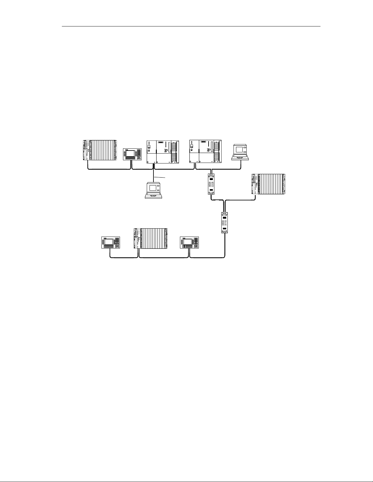
Figure 2-1 shows a typical topology using the RS-485 technique with 3 segments and 2 repeaters.

S7-400

OP 25



OP 25



 Terminating resistor activated  PG attached via tap line (6ES7 901-4BD00-0XA0)

for maintenance purposes

S7-300 S7-300

S7-400

Tap line



OP 25

RS-485 repeater



RS-485 repeater



S7-400



Figure 2-1 Topology Using the RS-485 Technique

Increasing the overall span of a network by using repeaters can lead to longer transmission times that may need to be taken into account when configuring the network (see Chapter 3).

2.1.1 Components for Transmission Rates up to 1.5 Mbps

All SIMATIC NET bus attachment components can be used for transmission rates ≤ 1.5 Mbps.

PROFIBUS Networks SIMATIC NET 6GK1970-5CA20-0AA1 Release 2 05/2000

2-3

Topologies of SIMATIC NET PROFIBUS Networks

2.1.2 Components for Transmission Rates up to

12 Mbps

The following bus attachment components can be used for transmission rates up to 12 Mbps:

Table 2-1 Bus Attachment Components for Transmission Rates up to 12 Mbps

Order number

PROFIBUS bus connector with

6GK1 500-0EA02

axial cable outlet PROFIBUS FastConnect bus connector RS-485

Plug 180 with 180° cable outlet 6GK1500-0FC00

RS-485 bus connector with vertical cable outlet Without PG interface With PG interface

6ES7 972-0BA11-0XA0 6ES7 972-0BB11-0XA0

PROFIBUS FastConnect RS-485 bus connector with 90° cable outlet with insulation displacement terminal system max. transmission rate 12 Mbps Without PG interface

6ES7 972-0BA50-0XA0 6ES7 972-0BB50-0XA0

With PG interface RS-485 bus connector with 35o cable outlet

Without PG interface With PG interface

6ES7 972-0BA40-0XA0 6ES7 972-0BB40-0XA0

SIMATIC NET 830-1T connecting cable, preassembled, fitted with terminating resistors, as link between electrical interface of an OLM or OBT and the PROFIBUS interface of a PROFIBUS node.

1.5 m 3 m

6XV1830-1CH15 6XV1830-1CH30

SIMATIC NET 830-2 connecting cable for PROFIBUS, preassembled cable with two sub-D, 9-pin male connectors, terminating resistors can be activated. 3 m 5 m 10 m

6XV1830-2AH30 6XV1830-2AH50 6XV1830-2AN10

SIMATIC S5/S7 PROFIBUS connecting cable for connecting programming devices up to 12 Mbps preassembled with 2 sub-D connectors, length 3 m 6ES7 901-4BD00-0XA0

PROFIBUS RS-485 repeater 24 V DC, casing with IP 20

6ES7 972-0AA01-0XA0

degree of protection Bus terminal BT12M 6GK1 500-0AA10 Optical Link Module OLM V3 6GK1 502-_C_00

PROFIBUS Networks SIMATIC NET

2-4

6GK1970-5CA20-0AA1 Release 2 05/2000

Topologies of SIMATIC NET PROFIBUS Networks

Table 2-1 Bus Attachment Components for Transmission Rates up to 12 Mbps, continued

Optical Bus Terminal OBT 6GK1 500-3AA0 PROFIBUS Terminator 6ES7 972-0DA00-0AA0

2.2 Topologies of Optical Networks

Interfacing Electrical and Optical Networks/Components

If you want to cover larger distances with the fieldbus regardless of the transmission rate or if the data traffic on the bus is threatened by extreme levels of external noise, you should use fiber-optic cables instead of copper cable.

To interface electrical cables with fiber-optic cables, you have the following possibilities:

S The PROFIBUS nodes with a PROFIBUS DP interface (RS-485) are attached

to the optical network using an optical bus terminal (OBT) or using an optical link module (OLM).

S PROFIBUS nodes with an integrated FO port (for example ET 200M (IM 153-2

FO), S7-400 (IM 467 FO)) can be connected directly to an optical network with a bus topology.

S Optical networks with a larger network span or structured as redundant rings

should be implemented using OLMs.

The structure of optical networks using optical link modules (OLMs) is described in detail in later chapters in this manual.

For information about the structure of an optical PROFIBUS network with PROFIBUS nodes having an integrated FO interface, refer also to the ET200 system manual.

PROFIBUS Networks SIMATIC NET 6GK1970-5CA20-0AA1 Release 2 05/2000

2-5

Topologies of SIMATIC NET PROFIBUS Networks

2.2.1 Topology with Integrated Optical Interfaces

The optical PROFIBUS network with nodes having an integrated FO interface is structured as a bus topology. The PROFIBUS nodes are interconnected in pairs by duplex fiber-optic cables.

Up to 32 PROFIBUS nodes with integrated FO interfaces can be connected in series in an optical PROFIBUS network. If a PROFIBUS node fails, the bus topology means that all DP slaves on the side away from the DP master are no longer obtainable for the DP master.

S7-400 with IM 467 FO

PG/PC/OP

Distances between 2

OBT

 Terminating resistor activated

1 FO cable 2 LAN cable for PROFIBUS

Figure 2-2 PROFIBUS DP Network with Nodes Having Integrated FO Interfaces

Plastic FO cable up to 50 m

PCF FO cable up to 300 m

nodes:

ET 200M with IM 153-2 FO

OBT

S7-300

For short distances, the preassembled 830-1T or 830-2 connecting cables can be used as an alternative to the PROFIBUS cable.

OP 25



other nodes

Transmission Rate

An optical PROFIBUS network with a bus topology can be operated at the following transmission rates:

9.6 Kbps, 19.2 Kbps, 45.45 Kbps, 93.75 Kbps, 187.5 Kbps, 500 Kbps, 1.5 Mbps and 12 Mbps

2-6

PROFIBUS Networks SIMATIC NET

6GK1970-5CA20-0AA1 Release 2 05/2000

PROFIBUS Optical Bus Terminal (OBT)

Using a PROFIBUS optical bus terminal (OBT), an individual PROFIBUS node without an integrated FO port or a PROFIBUS RS-485 segment can be attached to the optical PROFIBUS network (see Figure 2-2 ).

The attachment is made to the RS-485 interface of the OBT using a PROFIBUS cable or a preassembled connecting cable. The OBT is included in the optical PROFIBUS bus via the FO interface.

2.2.2 Topologies with OLMs

OLMs

The OLMs have a floating electrical channel (similar to the channels on a repeater) and depending on the version, they have one or two optical channels.

Topologies of SIMATIC NET PROFIBUS Networks

The OLMs are suitable for transmission rates of 9.6 Kbps to 12 Mbps. The transmission rate is detected automatically.

PROFIBUS Networks SIMATIC NET 6GK1970-5CA20-0AA1 Release 2 05/2000

2-7

Topologies of SIMATIC NET PROFIBUS Networks

Bus Topologies

Figure 2-3 shows a typical example of a bus topology In a bus structure, the individual SIMATIC NET PROFIBUS OLMs are connected

together in pairs by duplex fiber-optic cables. At the start and end of a bus, OLMs with one optical channel are adequate, in

between, OLMs with two optical channels are required. The DTEs are attached to the electrical interfaces of the OLMs. Either individual

DTEs or complete PROFIBUS segments with a maximum of 31 nodes can be connected to the RS-485 interface.



OP 25



ET 200M



ET 200S



OP 25



Bus connector

 Terminating resistor activated 1 FO cable 2 LAN cable for PROFIBUS 3 PROFIBUS 830-1T connecting cable 4 PROFIBUS 830-2 connecting cable

Figure 2-3 Example of a Bus Topology with OLMs

2-8

PROFIBUS Networks SIMATIC NET

6GK1970-5CA20-0AA1 Release 2 05/2000

Star Topologies with OLMs

Several optical link modules are grouped together to form a star coupler via a bus connection of the RS-485 interfaces. This RS-485 connection allows the attachment of further DTEs until the maximum permitted number of 32 bus attachments per segment is reached.

S7-400

OP 25



Topologies of SIMATIC NET PROFIBUS Networks

Star hub



S7-400

 Terminating resistor activated



1 FO cable 2 LAN cable for PROFIBUS 4 PROFIBUS 830-2 connecting cable

Figure 2-4 Example of a Star Topology with OLMs

Optical Channels

The OLMs are connected to the star coupler by duplex fiber-optic cables. Both DTEs and electrical bus segments can be connected to the OLMs attached

by the duplex fiber-optic cables. Depending on the requirements and the distance, the duplex cables can be implemented with plastic, PCF or glass (OLM only) fibers.



PROFIBUS Networks SIMATIC NET 6GK1970-5CA20-0AA1 Release 2 05/2000

2-9

Topologies of SIMATIC NET PROFIBUS Networks

Monitoring FO Links

Using the echo function, the connected OLMs can monitor the fiber-optic sections. A break on a link is indicated by a display LED and by the signaling contact responding.

Even if only one transmission direction is lost, the segmentation triggered by the monitoring function leads to safe disconnection of the OLM from the star coupler. The remaining network can continue to work without problems.

Mixed Structure

The star coupler can be made up with combinations of OLM/P, OLM/G and OLM/G-1300 modules and at the RS-485 end with all types.

Redundant Optical Rings using OLMs

Redundant optical rings are a special form of bus topology. By closing the optical bus to form a ring, a high degree of operational reliability is achieved

S7-400

OP 25

ET 200M



Path 1

Path 2

 Terminating resistor activated

1 FO cable 2 LAN cable for PROFIBUS

3 PROFIBUS 830-1T connecting cable 4 PROFIBUS 830-2 connecting cable

Figure 2-5 Network Structure in a Redundant, Optical, Two-Fiber Ring Topology



2-10

PROFIBUS Networks SIMATIC NET

6GK1970-5CA20-0AA1 Release 2 05/2000

Topologies of SIMATIC NET PROFIBUS Networks

A break on a fiber-optic cable between two modules is detected by the modules and the network is reconfigured to form an optical bus. The entire network remains operational.

If a module fails, only the DTEs or electrical segments attached to the module are separated from the ring; the remaining network remains operational as a bus.

The problem is indicated by LEDs on the modules involved and by their signaling contacts.

After the problem is eliminated, the modules involved cancel the segmentation automatically and the bus is once again closed to form a ring.

Note

To increase the availability, the duplex cables for the outgoing and incoming paths in the ring should be routed separately.

PROFIBUS Networks SIMATIC NET 6GK1970-5CA20-0AA1 Release 2 05/2000

2-11

Topologies of SIMATIC NET PROFIBUS Networks

Alternative Cabling Strategy

If the distance between two OLMs turns out to be too long, a structure as shown in Figure 2-6 can be implemented.



ET 200M

OP 25



OP 25



PG/PC/OP



S7-400



S7-400



 Terminating resistor activated

1 FO cable 2 LAN cable for PROFIBUS

3 PROFIBUS 830-1T connecting cable 4 PROFIBUS 830-2 connecting cable

Figure 2-6 Alternative Cabling of a Network Structure in an Optical Two-Fiber Ring Topology

PROFIBUS Networks SIMATIC NET

2-12

6GK1970-5CA20-0AA1 Release 2 05/2000

Topologies of SIMATIC NET PROFIBUS Networks

2.2.3 Combination of Integrated Optical Interfaces and OLMs

Note

Attaching Glass FO Cables to Buses Made up of Integrated Optical Interfaces

The operating wavelength of the integrated optical interfaces and the OBT is optimized for the use of plastic or PCF fibers. The direct attachment of glass FO cables is not possible.

If a link with glass FO cable is required, for example to span distances of more than 300 m, this link must be implemented with OLMs. The attachment of glass links to the optical bus made up of integrated optical interfaces is via the RS-485 interface of an OBT. The following schematic shows an example of an application:

ET 200M with



OBT



 Terminating resistor activated

1 FO cable 2 LAN cable for PROFIBUS

Figure 2-7 Attachment of an Optical Glass Link to an Optical Bus Made up of Integrated Optical

Interfaces

OBT



up to 15 km

IM 153-2 FO

OBT



3 PROFIBUS 830-1T connecting cable 4 PROFIBUS 830-2 connecting cable

Field device without FO interface

OBT



Further nodes

PROFIBUS Networks SIMATIC NET 6GK1970-5CA20-0AA1 Release 2 05/2000

2-13

Topologies of SIMATIC NET PROFIBUS Networks

2.3 Topologies of Wireless Networks

Infrared Link Module (ILM)

In SIMATIC NET, wireless PROFIBUS networks are implemented with the “Infrared Link Module (ILM)”.

Figure 2-8 PROFIBUS ILM

Maximum Length of a Link

Regardless of the transmission rate, the maximum length of a link is 15 m. The infrared light used for data transmission is radiated at an angle of +/- 10o around the mid axis. This means that at a distance of 11 m, an ILM illuminates a circular area with a diameter of 4 m. The communication partner must be within this illuminated area. There must be an uninterrupted line-of-sight path between both ILMs. The ILMs are suitable for transmission rates of 9.6 Kbps to 1.5 Mbps.

Point-to-Point Link

To implement a point-to-point link, two ILMs are positioned opposite each other so that each is located within the infrared light cone of the other. The maximum distance between two modules is 15 m.

2-14

PROFIBUS Networks SIMATIC NET

6GK1970-5CA20-0AA1 Release 2 05/2000

Master OP 25



Master PG/PC/OP

Topologies of SIMATIC NET PROFIBUS Networks

Infrared link

0.5 to 15 m

ILM ILM

Slave ET 200M

Master S7-400



Terminating resistor activated

2 LAN cable for PROFIBUS

Figure 2-9 Point-to-Point Link with Two PROFIBUS ILMs

PROFIBUS master network segment

Figure 2-9 illustrates the typical structure of a PROFIBUS network with master and slave nodes and an infrared link with two PROFIBUS ILMs. The infrared link is implemented as a point-to-point link between the two PROFIBUS ILMs. The two PROFIBUS ILMs replace a cable connection between the two network segments. Remember that only slave nodes are permitted in the slave network segment.



PROFIBUS slave network segment

Slave ET 200S



Point-to-Multipoint Link

Several ILMs are positioned opposite to a single ILM so that several ILMs are in the infrared light cone of another ILM. Only the ILMs positioned opposite each other can exchange data. A data exchange between adjacent ILMs is only possible by using a surface that reflects infrared light. If you consider this option, remember that the length of the link is the path from the ILM to the reflector and from the reflector to the partner ILM. Signal attenuation will also occur since the reflector can only reflect part of the infrared light to the partner ILM. Such losses mean a reduction in the maximum length of a link.

PROFIBUS Networks SIMATIC NET 6GK1970-5CA20-0AA1 Release 2 05/2000

2-15

Topologies of SIMATIC NET PROFIBUS Networks

Slave ET 200M



Master S7-400

Master PG/PC/OP

Master OP 25

Slave ET 200M



Slave S7-300

ILM



Infrared link 1

0.5 to 15 m



PROFIBUS slave network segment 1

Infrared

Slave ET 200M

ILM

link 2

0.5 to 15 m ILM



PROFIBUS slave network segment 2

Slave S7- 300

Infrared

link 3

0.5 to 15 m



Slave ET 200S

ILM



 Terminating resistor activated

2 LAN cable for PROFIBUS

PROFIBUS slave network segment 3

Figure 2-10 Point-to-Multipoint Link Using PROFIBUS ILMs (One Master Subnet, Three Subnets with

Slaves)

PROFIBUS Networks SIMATIC NET

2-16

6GK1970-5CA20-0AA1 Release 2 05/2000



Topologies of SIMATIC NET PROFIBUS Networks

2.4 Topologies with PROFIBUS-PA

Bus and Star Topology

With PROFIBUS-PA, the topology can be either a bus or star.

SpliTConnect System

The SpliTConnect tap (T tap) allows the structuring of a bus segment with DTE attachment points. The SpliTConnect tap can also be cascaded with the SpliTConnect coupler to form attachment distributors. Using the SpliTConnect terminator, the tap can be extended to become the segment terminator.

Star

Main cable

PROFIBUS-PA

DP/PA coupler (bus terminator integrated)

24 V DC

Figure 2-11 Bus and Star Topology

PROFIBUS-DP

T tap

Tap line

Field Device Power Supply via PROFIBUS-PA

When using the DP/PA bus coupler, the power for the field devices is supplied via the data line of PROFIBUS-PA.

Design

Tap line

Distributor made up of T taps

Bus

T tap with integrated bus terminator

Field devices attached via M12 connector

The total current of all field devices must not exceed the maximum output current of the DP/PA coupler. The maximum output current therefore limits the number of field devices that can be attached to PROFIBUS-PA.

PROFIBUS Networks SIMATIC NET 6GK1970-5CA20-0AA1 Release 2 05/2000

2-17

Topologies of SIMATIC NET PROFIBUS Networks

DP/PA coupler Ex [i] 6ES7 157-0AD00-0XA0

Protection EEx [ia] II C

x 90 mA

max

DP/PA coupler Ex [i] 6ES7 157-0AD80-0XA0

Protection EEx [ib] II C

x 110 mA

max

DP/PA coupler 6ES7 157-0ACx0-0XA0

x 400 mA

max

PROFIBUS-PA

max

24 V DC

PROFIBUS-DP

PROFIBUS-PA

max

24 V DC

PROFIBUS-DP

Field device

Field device2Field device

Explosion-protected area

Field device2Field device

3...

...I

Field device

...I

Field device

...n

...m

Figure 2-12 Field Device Power Supply in the Hazardous and Non-Hazardous Area

Expansion

If the maximum output current of the DP/PA coupler is exceeded, you must include a further DP/PA coupler.

Total Cable

The total cable is the total of the main cable and all the tap lines. When using a standard PROFIBUS-PA cable with a cross-sectional area of

0.8 mm2, the maximum length of the total cable (with a maximum number of field devices and worst-case positioning at the end of the cable) is as follows:

S 560 m for DP/PA coupler (6ES7 157-0AC00-0XA0) S 680 m for DP/PA coupler (6ES7 157-0AD80-0XA0) S 790 m for DP/PA coupler Ex [i] (6ES7 157-0AD00-0XA0)

Tap Line

The maximum permitted tap line lengths are listed in Table 2-2. You should also remember the maximum length of the total cable (see above).

2-18

PROFIBUS Networks SIMATIC NET

6GK1970-5CA20-0AA1 Release 2 05/2000

Topologies of SIMATIC NET PROFIBUS Networks

Table 2-2 Tap Line Lengths for DP/PA Couplers

Number of tap lines

1 to 12 max. 120 m max. 30 m 13 to 14 max. 90 m max. 30 m 15 to 18 max. 60 m max. 30 m 19 to 24 max. 30 m max. 30 m

Maximum length of the tap line

DP/PA coupler DP/PA coupler Ex [i]

PROFIBUS Networks SIMATIC NET 6GK1970-5CA20-0AA1 Release 2 05/2000

2-19

Topologies of SIMATIC NET PROFIBUS Networks

2.5 Connectivity Devices

2.5.1 DP/DP Coupler

Uses

The PROFIBUS-DP/DP coupler is used to link two PROFIBUS-DP networks together. Byte data (0 to 244 bytes) is transmitted from the DP master of a first network to the DP master of another network and vice-versa.

This principle corresponds to the hardware wiring of inputs and outputs. The coupler has two independent DP interfaces with which it attaches to the two DP networks.

The DP/DP coupler is a slave attached to the DP networks. The data exchange between the two DP networks involves internal copying within the coupler.

2-20

Figure 2-13 DP/DP Coupler

PROFIBUS Networks SIMATIC NET

6GK1970-5CA20-0AA1 Release 2 05/2000

Design

Topologies of SIMATIC NET PROFIBUS Networks

The DP/DP coupler is installed in a compact, 40 mm wide casing. The module can be installed (vertically when possible) on a standard rail with no

gaps being necessary. The coupler is attached to each PROFIBUS-DP network via an integrated 9-pin

sub-D connector.

Master OP 25



Master S7-400

SIEMENS

DP/DP COUPLER

Master PG/PC/OP



Terminating resistor activated



2 LAN cable for PROFIBUS

Figure 2-14 Configuration Example of the DP/DP Coupler

Master S7-300



Slave ET 200M



How the DP/DP Coupler Works

The DP/DP coupler permanently copies output data of one network to the input data of the other network (and vice-versa).

Parameter Assignment

The PROFIBUS-DP addresses are set using two DIP switches on the top of the device. The configuration is set using the GSD file and the configuration tool of the attached PROFIBUS-DP master. The data length is set with the relevant configuration tool.

PROFIBUS Networks SIMATIC NET 6GK1970-5CA20-0AA1 Release 2 05/2000

2-21

Topologies of SIMATIC NET PROFIBUS Networks

2.5.2 Connecting to PROFIBUS-PA

DP/PA Bus Coupling

The DP/PA bus coupler is the link between PROFIBUS-DP and PROFIBUS-PA. This means that it connects the process control systems with the field devices of the process automation (PA).

The DP/PA bus coupler is made up of the following modules:

S DP/PA Coupler Ex [i] (6ES7 157-0ADx0-0XA0) S DP/PA Coupler (6ES7 157-0ACx0-0XA0) S DP/PA Link IM 157 (6ES7 157-0AA80-0XA0)

To implement a DP/PA link in redundant operation, you also require the following:

S Bus module BM IM 157 for 2 x IM 157 (6ES7 195-7HE80-0XA0) S Bus module BM DP/PA Coupler for 1 DP/PA Coupler (6ES7 195-7HF80-0XA0)

2-22

PROFIBUS Networks SIMATIC NET

6GK1970-5CA20-0AA1 Release 2 05/2000

2.5.3 DP/PA Coupler

Figure 2-15 below illustrates how the DP/PA coupler is included in the system.

Process control level

Industrial Ethernet

Topologies of SIMATIC NET PROFIBUS Networks

“Programming, Operating and Monitoring”

SIMATIC PCS 7 or other tool for parameter assignment

PDM or other tool for parameter assignment

Cell level

Field level

Figure 2-15 Linking the DP/PA Coupler into the System

DP master

ET200X

PROFIBUS-DP

DP/PA coupler Ex [i]

Explosion-protected area

Uses of the DP/PA Coupler

The DP/PA coupler is available in two versions: S DP/PA coupler Ex [i]: You can attach all field devices certified for

PROFIBUS-PA and that are located within the hazardous area.

DP/PA coupler

PROFIBUS-PA

S DP/PA coupler: You can attach all field devices that are certified for

PROFIBUS-PA and that are outside the hazardous area.

The DP/PA coupler is an accompanying component according to EN 50014 or EN 50020 and must be installed outside the hazardous area.

PROFIBUS Networks SIMATIC NET 6GK1970-5CA20-0AA1 Release 2 05/2000

2-23

Topologies of SIMATIC NET PROFIBUS Networks

Properties of the DP/PA Coupler (General)

The DP/PA coupler has the following characteristics:

S Electrical isolation between PROFIBUS-DP and PROFIBUS-PA S Conversion of the physical transmission mechanism between RS-485 and IEC

61158-2

S Diagnostics using LEDs S Transmission rate on PROFIBUS-DP 45.45 Kbps S Transmission rate on PROFIBUS-PA 31.25 Kbps S Integrated power supply unit

Properties of the DP/PA Coupler Ex [i]

The DP/PA coupler Ex [i] (6ES7 157-0AD00-0XA0) has the following additional characteristics:

S Type of Protection EEx [ia] II C S Intrinsic safety S Integrated, intrinsically safe power supply unit and integrated barrier

The DP/PA coupler Ex [i] (6ES7 157-0AD80-0XA0) has the following characteristics that differ from the DP/PA coupler EX [i] (6ES7 157-0AD00-0XA0):

S Type of protection EEx [ib] II C S Extended environmental conditions (SIMATIC outdoor)

Configuring the DP/PA Coupler

S The DP/PA coupler can be used in SIMATIC S5 and S7 and with all DP masters

that support 45.45 Kbps.

S The DP/PA coupler does not need to be configured. You must only set the

transmission rate of 45.45 Kbps for the relevant DP network during configuration. You then configure the PA field devices just as normal DP slaves using the DP configuration tool and the appropriate GSD file. You can configure the PA field devices with SIMATIC PDM or with any other vendor-specific software configuration tool.

2-24

PROFIBUS Networks SIMATIC NET

6GK1970-5CA20-0AA1 Release 2 05/2000

2.5.4 DP/PA Link

Definition

The DP/PA link consists of the IM 157 and up to a maximum of five DP/PA couplers. The DP/PA link is a DP slave at the PROFIBUS-DP side and a PA master at the PROFIBUS-PA side.

Uses

With the DP/PA link, you have an isolated interconnection between PROFIBUS-PA and PROFIBUS-DP with transmission rates of 9.6 Kbps to 12 Mbps.

The DP/PA link can only be used in SIMATIC S7. Figure 2-16 below shows where the DP/PA link fits in.

Topologies of SIMATIC NET PROFIBUS Networks

Process control level

S7-DP master

Gateway S7-400

Cell level

Field level

Figure 2-16 Location of the DP/PA Link

Industrial Ethernet

PROFIBUS-DP

ET200X

“Programming, Operating and Monitoring”

SIMATIC PCS 7 or other tool for parameter assignment

PDM or other tool for parameter assignment

DP/PA Link

DP/PA coupler

12 34 5

IM 157

PROFIBUS-PA

Field devices of PROFIBUS-PA

The DP/PA link must be installed outside the hazardous area. The DP/PA link is configured with STEP 7, Version 4.02 or higher.

PROFIBUS Networks SIMATIC NET 6GK1970-5CA20-0AA1 Release 2 05/2000

2-25

Topologies of SIMATIC NET PROFIBUS Networks

Properties

The DP/PA link has the following characteristics:

S Diagnostics with LEDs and the user program S DP slave and PA master S Can be operated at all transmission rates (9.6 Kbps to 12 Mbps) S Only DP/PA couplers can be operated with an IM 157

How the DP/PA Link Works

Figure 2-17 shows how the DP/PA link with the IM 157 and the DP/PA couplers functions.

S The DP/PA link maps the underlying PROFIBUS-PA system on a DP slave. S With the DP/PA link, PROFIBUS-DP is completely isolated from

PROFIBUS-PA.

S The PA master and PA slaves form a separate, underlying bus system. S The number of DP/PA couplers simply reflects the amount of current required.

All DP/PA couplers along with the attached PA field devices form one common PROFIBUS-PA bus system.

DP/PA Link

IM 157

DP slave

DP/PA coupler (max. 5)

S7 backplane bus

PA PA

P A master

2-26

Figure 2-17 The DP/PA Link with DP/PA Couplers

PROFIBUS Networks SIMATIC NET

6GK1970-5CA20-0AA1 Release 2 05/2000

Rules

Topologies of SIMATIC NET PROFIBUS Networks

The following rules must be taken into account when extending PROFIBUS-PA:

S There can be a maximum of 31 PA field devices in a PROFIBUS-PA system S Only one device supplying power (=DP/PA coupler) can be connected in a

physical PROFIBUS-PA segment.

S A maximum of 31 PA field devices can be attached to a DP/PA link. The

maximum number of attachable PA field devices per physical PROFIBUS-PA segment or per DP/PA coupler is limited by the maximum output current of the DP/PA coupler and the I/O data to be transferred.

PROFIBUS Networks SIMATIC NET 6GK1970-5CA20-0AA1 Release 2 05/2000

2-27

Topologies of SIMATIC NET PROFIBUS Networks

2.5.5 Connecting PROFIBUS-DP to RS-232C

Design

Figure 2-18 DP/RS-232C Link for PROFIBUS-DP

The DP/RS-232C link consists of a compact 70 mm housing for standard rail mounting. Ideally the module should be installed vertically. The modules can be inserted one beside the other without gaps being necessary. The module is attached to PROFIBUS-DP via a 9-pin sub-D female connector. The RS-232C interface is implemented as a 9-pin sub-D connector.

2-28

PROFIBUS Networks SIMATIC NET

6GK1970-5CA20-0AA1 Release 2 05/2000

Uses

Topologies of SIMATIC NET PROFIBUS Networks

The PROFIBUS-DP/RS-232C link is a converter between an RS-232C (V.24) interface and PROFIBUS-DP. Devices with an RS-232C interface can be linked to PROFIBUS-DP with the DP/RS-232C link. The DP/RS-232C link supports the procedures 3964 R and free ASCII protocol.

Master S7-400

SIEMENS

Configuration with STEP 7

PROFIBUS-DP

PROFIBUS LAN cable

DP/RS-232C Link

Figure 2-19 Example of a Configuration with DP/RS-232C Link

How the DP/RS-232C Link Works

The PROFIBUS-DP/RS-232C link is connected with the device over a point-to-point connection. The PROFIBUS-DP/RS-232C link converts to the PROFIBUS-DP protocol. Consistent data are transferred in both directions. A maximum of 224 bytes of user data can be transferred per frame.

PROFIBUS Networks SIMATIC NET 6GK1970-5CA20-0AA1 Release 2 05/2000

Device

RS-232C

Serial procedure

2-29

Topologies of SIMATIC NET PROFIBUS Networks

Parameter Assignment

The PROFIBUS-DP address can be set using two switches on the front panel. To configure the unit, you use the GSD file and the configuration tool of the connected device, for example STEP 7.

2.5.6 Connecting with the DP/AS-Interface Link 65

Design

Figure 2-20 DP/AS-Interface Link 65

The DP/AS-interface link has a robust aluminum die-cast casing with the degree of protection IP 65. In terms of water tightness, it complies with the standard “Enclosures for Electrical Equipment UL 50, Type 4”, and is suitable for temperatures from -25 °C to +60 °C. On the casing, there are diagnostic LEDs for PROFIBUS-DP and the AS interface. The node address for PROFIBUS-DP can be set using DIL switches or using an EEPROM. To set the address using the EEPROM, you can use the ET 200 handheld. The DP/AS-interface link can be installed anywhere and in any position. The attachment to PROFIBUS-DP is via a 12-pin round connector, the attachment to AS-interface is via a 4-pin modular connector (M12 AS-interface attachment).

2-30

PROFIBUS Networks SIMATIC NET

6GK1970-5CA20-0AA1 Release 2 05/2000

Uses

Topologies of SIMATIC NET PROFIBUS Networks

The DP/AS-interface link connects the PROFIBUS-DP fieldbus with the AS-interface. The DP/AS-interface link 65 can be connected to any PROFIBUS-DP master capable of handling parameter assignment and diagnostic frames with a length of 32 bytes. The DP/AS-interface link 65 allows the actuator-sensor interface to be used as a subnet for PROFIBUS-DP. You can therefore combine the advantages of PROFIBUS-DP and AS-interface in a common bus system.

Field level networking with PROFIBUS-DP

External power supply 24 V DC

DP/AS-Interface Link 65

Passive modules (without slave ASIC)

Active modules

(with slave ASIC)

AS-i power supply

Actuator/sensor with slave ASIC

AS-i cable

Figure 2-21 Example of a Configuration with DP/AS-Interface Link 65

Branch

PROFIBUS Networks SIMATIC NET 6GK1970-5CA20-0AA1 Release 2 05/2000

2-31

Topologies of SIMATIC NET PROFIBUS Networks

How the DP/AS-Interface Link 65 Works

The DP/AS-interface link 65 links PROFIBUS-DP with the AS-interface with degree of protection IP 65. The DP/AS-interface link 65 can be connected to any PROFIBUS-DP master that can send parameter assignment frames with a length of 32 bytes. To act as a connectivity device between the two bus systems, the DP/AS-interface link has the functionality of an AS-interface master towards the AS-interface and the functionality of a PROFIBUS-DP slave towards PROFIBUS-DP. Up to 31 DP/AS-interface slaves can be attached to the DP/AS-interface link. The DP/AS-interface link is therefore a modular slave with up to 31 modules from the point of view of PROFIBUS-DP.

Parameter Assignment

Like all other components of the distributed I/O system ET 200, the DP/AS-interface link is an integral part of STEP 7 and COM PROFIBUS. You can display information about working with the parameter assignment software and configuring at any time using the context-sensitive help.

2-32

PROFIBUS Networks SIMATIC NET

6GK1970-5CA20-0AA1 Release 2 05/2000

Topologies of SIMATIC NET PROFIBUS Networks

2.5.7 Connecting with the DP/AS-Interface Link 20

Design

Figure 2-22 DP/AS-Interface Link 20

The DP/AS-interface link 20 consists of a small, compact casing with degree of protection IP20. The LEDs on the front panel indicate the following:

S AS-Interface statuses S Attached and active slaves and their operability S PROFIBUS slave address S PROFIBUS bus errors and diagnostics

The DP/AS-interface link 20 also has a button with which the operating mode can be changed, with which the existing configuration can be adopted and for setting the PROFIBUS slave address.

PROFIBUS Networks SIMATIC NET 6GK1970-5CA20-0AA1 Release 2 05/2000

2-33

Topologies of SIMATIC NET PROFIBUS Networks

Uses

The DP/AS-interface link 20 implements a small, cost-effective link between PROFIBUS and AS-interface. The DP/AS-interface link 20 requires no additional power supply, the power is supplied on the AS-interface cable. The AS-interface segment can be started up without PROFIBUS-DP being in operation.

The DP/AS-interface link 20 is a PROFIBUS-DP slave (complying with EN 50170) and AS-interface master in one unit and provides a simple link between PROFIBUS-DP and the AS-interface. The DP/AS-interface link 20 allows system attachment of the following:

S PROFIBUS-DP master, for example CP 342-5 for S7-300, CP 443-5 extended

for S7-400, CP 5431 FMS/DP or IM 308C for SIMATIC S5, CP 5412 (A2) for PC or CP 5611/CP 5511 for PCs with DP-SOFTNET software.

S Other systems with DP master functionality

Field level networking with PROFIBUS-DP

AS-i power supply

Actuator/sensor with slave ASIC

ADR

DP/AS-Interface

Link 20

DIA

APF

CER AUP

0910

6GK7 1415 2AA0

DP/AS-Interface Link 20

Passive modules (without slave ASIC)

AS-i cable

X 2 34

Active modules

(with slave ASIC)

Branch

Figure 2-23 Example of a Configuration with DP/AS-Interface Link 20

2-34

PROFIBUS Networks SIMATIC NET

6GK1970-5CA20-0AA1 Release 2 05/2000

How the DP/AS Interface Link 20 Works

With the DP/AS-interface link 20, up to 248 binary elements are accessible to a DP master on the AS-interface (124 inputs and 124 outputs). You can therefore combine the advantages of PROFIBUS-DP and AS-interface in a plant. The DP/AS-interface link 20 can be used in the AS-interface standard mode (M2). In this mode, the data bits of the slaves are accessible. The following master calls are supported.

S Change address S Write parameters S Read configuration data S Set configuration mode S Configure actual configuration

Parameter Assignment

The DP/AS-interface link 20 is supported by STEP 7 (V4.1 and higher) and COM PROFIBUS (V 3.2 and higher). The type and GSD files are shipped along with the manual. On the AS-interface side, no special configuration is necessary; the AS-Interface segment can be put into operation without PROFIBUS.

Topologies of SIMATIC NET PROFIBUS Networks

PROFIBUS Networks SIMATIC NET 6GK1970-5CA20-0AA1 Release 2 05/2000

2-35

Topologies of SIMATIC NET PROFIBUS Networks

2.5.8 Connecting PROFIBUS-DP to instabus EIB

Design

Uses

Figure 2-24 DP/EIB Link

The DP/EIB link allows a connection between the two open standard systems for industrial automation PROFIBUS-DP and building automation instabus EIB. This provides an ideal connection between the high performance of the PROFIBUS components and the extreme flexibility of the instabus EIB system.

The DP/EIB link is a DP slave (complying with EN 50170) and at the same time a node on the instabus EIB.

The displays and operating controls are as follows:

S LED for EIB bus errors S LED for PROFIBUS bus errors S LED for power supply OK S Coding switch for the PROFIBUS address S Programming button for EIB.

The DP/EIB link can be used wherever PROFIBUS or instabus EIB is used; in other words, a distinction can be made between two areas of application:

2-36

PROFIBUS Networks SIMATIC NET

6GK1970-5CA20-0AA1 Release 2 05/2000

Building Automation

In other words, we are assuming that instabus EIB exists and that you want to use, for example, an S7 PLC for administrative control tasks or, for example, an HMI system for central operator control and monitoring. The main emphasis here is in offices or apartment blocks etc.

The simplest option for connecting these systems to instabus EIB is provided by the DP/EIB link since these systems generally access the peripheral devices via PROFIBUS.

The main areas of application are as follows: S (Primary) open-loop control, closed-loop control and monitoring of heating

systems

S Ventilation, air-conditioning, and S Energy management and optimization

Industrial Automation

Topologies of SIMATIC NET PROFIBUS Networks

In this case, we assume that PROFIBUS exists and that you would like to include the electrical components of an assembly line, plant or production building in the automation. The main emphasis here is the equipment of industrial buildings themselves.

Applications include, for example, the following:

S lighting control S shutter control, S measurement of temperature, wind strength, or the position of the sun, S door control and S building access controls.

The instabus EIB is specifically designed for such tasks and provides a wide selection of components and a large network span (maximum 1000 m per bus). Up to 11,520 instabus EIB devices are possible in one network (a maximum of 15 areas each with a maximum of 12 buses each with up to 64 nodes).

PROFIBUS Networks SIMATIC NET 6GK1970-5CA20-0AA1 Release 2 05/2000

2-37

Topologies of SIMATIC NET PROFIBUS Networks

Step 7 or COM PROFIBUS

EIBRS-232 interface

S7-300 ET 200S

PROFIBUS

ET 200M

instabus EIB

ETS2

Figure 2-25 Example of a System Structure using DP/EIB Link

How the DP/EIB Link Works

The data objects of the instabus EIB are mapped in the PROFIBUS I/O area. The structuring of the PROFIBUS slave I/O area and the number of EIB data

objects with which the DP master communicates is decided by a selectable profile. In total, five different profiles are available that allow the user to adapt the DP/EIB link to the relevant application and to make optimum use of the memory resources of the DP master.

You configure the system (in other words set a profile) via PROFIBUS using, for example STEP 7 or COM PROFIBUS. The number of data objects specified by the selected profile can be assigned to the required instabus EIB components with the instabus EIB configuration software ETS 2.

Due to the database entry of the DP/EIB link, the instabus EIB configuration software ETS 2 is capable of displaying the number and data type of the valid instabus EIB data objects to the user. This allows a simple error-free assignment to be made. Following configuration, the PROFIBUS-DP master can both write and read the instabus EIB data objects.

Siemens EIB product database

2-38

PROFIBUS Networks SIMATIC NET

6GK1970-5CA20-0AA1 Release 2 05/2000

Configuring

Topologies of SIMATIC NET PROFIBUS Networks

The link module can be configured as a DP slave, for example with the standard tools STEP 7 or COM PROFIBUS and on the instabus EIB using the configuration software ETS 2.

S DP

A GSD file is supplied with the manual. The DP slave address is set with a coding switch on the DP/EIB link.

S instabus EIB

The database entry of the DP/EIB link for instabus EIB configuration software ETS 2 is supplied with the DP/EIB manual.

For further details, refer to the DP/EIB link manual.

PROFIBUS Networks SIMATIC NET 6GK1970-5CA20-0AA1 Release 2 05/2000

2-39

Topologies of SIMATIC NET PROFIBUS Networks

2-40

PROFIBUS Networks SIMATIC NET

6GK1970-5CA20-0AA1 Release 2 05/2000

Configuring Networks

PROFIBUS Networks SIMATIC NET 6GK1970-5CA20-0AA1 Release 2 05/2000

3-1

Configuring Networks

3.1 Configuring Electrical Networks

PROFIBUS Networks

PROFIBUS networks were specially designed for use in an industrial environment and one of their main features is their degree of immunity to electromagnetic interference resulting in high data integrity. To achieve this degree of immunity, certain guidelines must be adhered to when configuring electrical networks.

Parameters

The following parameters must be taken into account when planning an electrical network:

S The transmission rate required for the task

(within a network, only one uniform transmission rate can be used)

S The required number of nodes S The type of network components required (bus terminals, bus connectors,

connecting cables)

S The LAN cables to be used S The required segment lengths S The electromagnetic and mechanical environment of the cabling (for example

surge voltage protection, cable route)

S The number of RS-485 repeaters between any two DTEs is limited to a

maximum of 9

S Increasing the overall span of a network by using repeaters can lead to longer

transmission times that may need to be taken into account when configuring the network (see Section 3.3).

Cable Termination

Regardless of the transmission rate, the ends of all segments must be terminated by activating the terminating resistor in the connector. After the terminating resistor has been activated, no further cable sections are permitted.

The terminating resistor is only effective when it is supplied with voltage. This means that the corresponding DTE or the RS-485 repeater must be supplied with power. As an alternative, the PROFIBUS terminator can be used as a permanent terminating resistor.

3-2

PROFIBUS Networks SIMATIC NET

6GK1970-5CA20-0AA1 Release 2 05/2000

Configuring Networks

Note

The power supply to terminating resistors must not be interrupted by turning off the DTE or repeater or by unplugging the bus connector or tap line. If the power supply to the terminating resistors cannot be guaranteed, the PROFIBUS terminator must be used.

3.1.1 Segments for Transmission Rates up to a Maximum of 500 Kbps

Transmission Rates up to a Maximum of 500 Kbps

The following maximum segment lengths can be implemented with the SIMATIC NET PROFIBUS LAN cables:

Table 3-1 Possible Segment Lengths

Segment Length for Cable Type

Transmission Rate in Kbps

9.6 1000 m 900 m

19.2 1000 m 900 m

45.45 1000 m 900 m

93.75 1000 m 900 m

187.5 1000 m 700 m 500 400 m 400 m

– FC Standard Cable – FC Robust Cable – FC FRNC Cable – FC Food Cable – FC Underground Cable – SIENOPYR–FR Marine Cable

– FC Trailing Cable – PROFIBUS Flexible Cable – PROFIBUS Festoon Cable

The maximum permitted number of bus attachments (DTEs, repeaters, OLMs, BT12 M,...) to one segment is 32.

PROFIBUS Networks SIMATIC NET 6GK1970-5CA20-0AA1 Release 2 05/2000

3-3

Configuring Networks

Length of the Tap Lines

If you do not attach the LAN cable directly to the bus connector (for example,when using a PROFIBUS bus terminal), you must take into account the maximum possible tap line length!

The following table shows the maximum permitted lengths of tap lines per bus segment:

Table 3-2 Lengths of the Tap Lines per Segment

Transmission

rate

Max. length of the tap lines per segment

Number of nodes with tap line length of ...

1.5 m or 1.6 m 3 m

9.6 – 93.75 Kbps 96 m 32 32

187.5 Kbps 75 m 32 25 500 Kbps 30 m 20 10

3.1.2 Segments for a Transmission Rate of 1.5 Mbps

Transmission Rate 1.5 Mbps

The following maximum segment length can be implemented with the SIMATIC NET PROFIBUS LAN cable:

Table 3-3 Possible Segment Lengths

Segment Length for Cable Type

Transmission Rate in Kbps

1.500 200 m 200 m

– FC Standard Cable – FC Robust Cable – FC FRNC Cable – FC Food Cable – FC Underground Cable – SIENOPYR–FR Marine Cable

– FC Trailing Cable – PROFIBUS Flexible Cable – PROFIBUS Festoon Cable

Node Attachments at 1.5 Mbps

Each attachment of a node to the LAN cable represents a capacitive mismatch that has no effect at lower transmission rates. At a transmission rate of 1.5 Mbps, however, problems can arise due to these mismatches if the following guidelines in terms of type, number and distribution of node attachments are not adhered to.

3-4

PROFIBUS Networks SIMATIC NET

6GK1970-5CA20-0AA1 Release 2 05/2000

Configuring Networks

Value Factors

To be able to define permitted configurations, a method is necessary with which the attached components can be evaluated in terms of their capacitive bus load. This is achieved by assigning value factors to the components (see Table 3-4 ).

PROFIBUS interfaces implemented as 9-pin sub-D female connectors (CPs, OLMs...), do not have their own value factors. These are already taken into account in the values listed in the table.

Table 3-4 Values for Segments at 1.5 Mbps

Product Name V alue (V) Bus terminal with 1.5 m long tap line

(Order no. 6GK1 500-0AA00, Version 2) Bus terminal with 1.5 m long tap line, with PG interface

(Order no. 6GK1 500-0DA00, Version 2) Bus terminal with 3.0 m long tap line

(Order no. 6GK1 500-0BA00, Version 2) Bus connector with 30° cable outlet

(Order no. 6ES7 972-0BA30-0XA0) Bus connector with axial cable outlet (Order no.: 6GK1 500-0EA02)

Bus connector with axial cable outlet for FastConnect system (Order no.: 6GK1 500-0FC00) Bus connector with 90° cable outlet (Order no.: 6ES7 972-0BA11-0XA0) Bus connector with 90° cable outlet with PG interface (Order no.: 6ES7 972-0BB11-0XA0) Bus connector with 90° cable outlet for FastConnect system (Order no.: 6ES7

972-0BA50-0XA0)

Bus connector with 90° cable outlet with PG interface (Order no.: 6ES7 972-0BB50-0XA0) Bus connector with 35° cable outlet (Order no.: 6ES7 972-0BA40-0XA0) Bus connector with 35° cable outlet with PG interface

(Order no.: 6ES7 972-0BB40-0XA0)

Bus terminal BT12M (Order no. 6GK1500-0AA10) 0.1 RS-485 repeater (attachment of bus segments) (Order no. 6ES7 972-0AA01-0XA0) 0.1 PROFIBUS terminator (active RS-485 attachment element)

(Order no. 6ES7 972-0DA01-0AA0) SIMATIC S5/S7 connecting cable for 12 Mbps PG attachment to PROFIBUS-DP (Order

no.: 6ES7 901-4BD00-0XA0)

1.5

2.5

0.7

0.1

0.5

PROFIBUS Networks SIMATIC NET 6GK1970-5CA20-0AA1 Release 2 05/2000

3-5

Configuring Networks

Rules

At a transmission rate of 1.5 Mbps, the following rules apply to the permitted number of nodes and their distribution/layout on a SIMATIC NET PROFIBUS segment:

1. The maximum permitted number of nodes on any segment is 32.

2. The sum of the values of all the connection elements in a segment must be ≤ 25.

3. The rules for the distance between adjacent connection elements are as follows (distance in this case is the length of the LAN cable):

3.1 If the distance between adjacent connection elements is greater than

3.2 If the distance between adjacent connections elements is greater than the

10 m, the values of the connection elements can be ignored.

sum of the two values of the elements in meters, the layout is not critical and no additional conditions need to be taken into account. The value of the PG connecting cable, SIMATIC S5/S7 connecting cable 12 Mbps must be added to the value of the corresponding connection element.

3.3 If the minimum clearance described in 3.2 is not kept to, this results in

a group being formed and the following additional conditions must be met:

– Attachment elements can be arranged as close to each other as

required providing the sum of their values does not exceed the value 5.

– The distance in meters between two adjacent groups must be at least

as large as the sum of the values of the two groups.

3-6

PROFIBUS Networks SIMATIC NET

6GK1970-5CA20-0AA1 Release 2 05/2000

Table 3-5 Examples Illustrating the Configuration Rules

Configuring Networks

No special conditions if the length of the LAN cable between two DTEs > 10 m

No special conditions if the length of the LAN cables between two DTEs is greater than the sum of values of both DTEs.

If a bus terminal or a bus connector has a PG interface, a connected PG connecting cable must be taken into account when calculating the values.

Take the values of a group into account if the sum of the values is greater than the LAN cable between the DTEs.

Elements can be close to each other providing the total value of a group does not exceed 5.

LAN cable > 10 m

> 10 m

S7-400

S7-300

Bus cable, e.g. 5 m V = 1.5 + 1.0 + 0.1 = 2.6 5 m > 2.6 m (sum of the values in

meters)

S7-400

V = 1.0

5 m

V = 1.5

V = 0.1

S7-300

LAN cable e.g. 0.5 m group V = 1.5 + 1.5

0.5 m < 3 m ⇒ group formed ⇒ sum of the values ≤ 5

S7-400

PROFIBUS Networks SIMATIC NET 6GK1970-5CA20-0AA1 Release 2 05/2000

V = 1.5

0.5 m

V = 1.5

3-7

Configuring Networks

3.1.3 Segments for Transmission Rates up to a Maximum of 12 Mbps

Transmission Rate up to a Maximum of 12 Mbps

Table 3-6 Possible Segment Lengths

Segment Length for Cable Type

Transmission Rate in Mbps

3 100 m 100 m 6 100 m 100 m 12 100 m 100 m

– FC Standard Cable – FC Robust Cable – FC FRNC Cable – FC Food Cable – FC Underground Cable – SIENOPYR–FR Marine Cable

– FC Trailing Cable – PROFIBUS Flexible Cable – PROFIBUS Festoon Cable

When planning segments for transmission rates from 3 Mbps to a maximum of 12 Mbps, the following factors must be taken into account:

S To attach DTEs to bus segments, only the bus connectors permitted for 12

Mbps or the BT12M bus terminal can be used.

S The maximum length of a segment must not exceed 100 m. S The maximum number of bus attachments (nodes, OLMs, RS-485 repeaters,...)

in one segment is restricted to 32.

S To attach a programming device or PC via a tap line, only the “SIMATIC S5/S7

connecting cable, 12 Mbps, order no. 6ES7901-4BD00-0XA0” can be used.

Note

If several bus connectors are used at electrically short distances (in other words, the cable length between adjacent connectors is less than 1 m) (for example, several slaves in one cubicle), avoid disconnecting several bus connectors at the same time for longer periods. Disconnecting more than one bus connector does not necessarily mean errors but may well reduce the reliability (immunity to noise) of a segment.

3-8

PROFIBUS Networks SIMATIC NET

6GK1970-5CA20-0AA1 Release 2 05/2000

Configuring Networks

3.1.4 Configuring Electrical Networks with RS-485 Repeaters

RS-485 Repeater

To increase the number of nodes (>32) in a network or to extend the cable length between two nodes, segments can be connected together using RS-485 repeaters to form a network. Figure 3-1 illustrates how several segments can be connected together with repeaters to create a network.

The RS-485 repeaters support all transmission rates from

9.6 Kbps to 12 Mbps.

S7-300

ET200S



OP 25



OP 25

ET200M

OP 25

S7-300

RS-485 repeater



S7-300



OP 25



ET200M

ET200S



OP 25

 Terminating resistor activated

Figure 3-1 Layout of an Electrical PROFIBUS Network Using RS-485 Repeaters

PROFIBUS Networks SIMATIC NET 6GK1970-5CA20-0AA1 Release 2 05/2000

3-9

Configuring Networks

Configuring

When configuring an electrical network with RS-485 repeaters, the following conditions must be taken into account:

S The maximum segment length for the transmission rate must be adhered to

(see Table 3-1, Table 3-3, Table 3-6,)

S The maximum number of bus attachments (nodes, OLMs, RS-485 repeaters,...)

in one segment is restricted to 32. There may be further restrictions at a transmission rate of 1.5 Mbps (see Section 3.1.2).

S The maximum number of nodes in one network is limited to 127. S A maximum of 9 RS-485 repeaters can be installed between two nodes.

3-10

PROFIBUS Networks SIMATIC NET

6GK1970-5CA20-0AA1 Release 2 05/2000

3.2 Configuring Optical Networks

Configuration Parameters for Optical Networks

When configuring optical PROFIBUS networks, the following parameters must be taken into account:

S Using fiber-optic cables, only point-to-point links can be established. S The maximum signal attenuation of the transmission path (the power budget)

must be within the permitted values.

S The minimum or maximum permitted transmission rates of the components

(only one uniform transmission rate can be used in a network).

S The cascading rules for the components used. S The maximum permitted number of nodes in the network. S In large-span networks, the transmission delay time.

Configuring Networks

PROFIBUS Networks SIMATIC NET 6GK1970-5CA20-0AA1 Release 2 05/2000

3-11

Configuring Networks

3.2.1 How a Fiber-Optic Cable Transmission System Works

Introduction

This section describes the structure and functions of an optical transmission system. The information here will help you to understand the rules for calculating the optical power budget in the next section.

Transmission Path

An optical transmission path consists of a transmitter, the optical fiber, and a receiver.

Power supply

Signal converter

Electr . signal (digital/analog)

Figure 3-2 Structure of a Link

E / O converter

Transmitter

The transmitter in an optical digital transmission system consists of a signal converter that converts the digital signals from the electronics in to a pulse type suitable for the electro-optical converter, and an electro-optical converter (E/O converter) that converts the electric pulses to optical signals. In SIMATIC NET PROFIBUS, LEDs (LED = Light Emitting Diode) are used as E/O converters. The LEDs are specially adapted to the various transmission media.

Optical fiber

Attenuation transmission path

E/O = Electro-optical converter O/E = Optoelectrical converter

O / E converter

Power supply

Signal converter

Electr . signal (digital/analog)

Transmission Media

The transmission media used in SIMATIC NET PROFIBUS are as follows:

S Plastic fiber-optic cables S PCF fiber-optic cables (polymer cladded fiber) S Glass fiber-optic cables

For more detailed information about the various fiber-optic cables for SIMATIC NET PROFIBUS, refer to Chapter 7.

3-12

PROFIBUS Networks SIMATIC NET

6GK1970-5CA20-0AA1 Release 2 05/2000

Receiver

Attenuation

Configuring Networks

The receiver of a digital optical transmission system consists of an optoelectric converter (a photodiode), that converts the optical signals to electrical signals and a signal converter that converts the electrical pulses received from the diode into signals compatible with the connected electronics.

The attenuation of the transmission path is determined by the following factors:

S The choice of optical fiber S The wavelength of the transmit diodes S The type of connector S With glass optical fibers, the number of splices (including repair splices) S The length of the optical fiber (cable length) S The link power margin on the link (for example for aging and temperature

dependency of the LEDs and photodiodes).

PROFIBUS Networks SIMATIC NET 6GK1970-5CA20-0AA1 Release 2 05/2000

3-13

Configuring Networks

3.2.2 Optical Power Budget of a Fiber-Optic Transmission System

Optical Power Budget

Transmitter

The transmitted optical power P

and the received optical power P

out

rec

are specified in dBm, the attenuation caused by connectors and the fiber is specified in dB.

dBm is a reference unit and describes the logarithmic ratio of the power level to the reference power P0=1mW. The following formula applies:

Px [in dBm] = 10*log(Px [in mW] / P0)

Examples:

Transmitter Power PxTransmitter Power as Logarithmic Power

10 mW 1 mW 1

µW

Ratio Px to P

+ 10 dBm 0 dBm – 30 dBm

Depending on the fiber being used, the minimum and maximum optical power that can be coupled into a fiber is specified. This power is reduced by the attenuation of the connected transmission path resulting from the fiber itself (length, absorption, scattering, wavelength) and the connectors used.

Receiver

3-14

The receiver is characterized by its optical sensitivity and its dynamic range. When configuring an optical link, you should make sure that the power reaching the receiver does not exceed its dynamic range. If the power falls below the minimum, this increases the bit error rate (BER) due to the signal-to-noise ratio of the receiver. If the maximum received power is exceeded, saturation and overload effects increase pulse distortion and therefore also increase the bit error rate.

PROFIBUS Networks SIMATIC NET

6GK1970-5CA20-0AA1 Release 2 05/2000

Power Budget

The power budget of an optical link not only takes into account the attenuation in the fiber itself, temperature and aging effects but also the attenuation values of the connectors and splices and therefore provides exact information about whether or not an optical link can be implemented. The starting point for calculating the maximum transmission path length is the minimum transmitter power that can be coupled into the fiber type. To simplify matters, the budget is calculated in dBm and dB.

The following is subtracted from the minimum transmitter power:

Configuring Networks

S The attenuation of the fiber a S The input power required at the receiver

The coupling losses at the send and receive diodes are already taken into account in the information about the transmitter power and receiver sensitivity.

Plastic and PCF FO Cables

Plastic and PCF FO cables can only be used on short distances due to their relatively high fiber attenuation. They are installed in one piece. Fiber-optic connections with couplers or splices should not be considered since they further reduce the distance that can be covered. The maximum permitted cable lengths are listed in Tables 3-7 and 3-8.

Glass FO Cables

Glass FO cables can span distances in the kilometer range. It is often not possible to install cables over such distances in one piece. The fiber-optic path must then be put together in cable sections. The couplers or splices where the sections are joined always involve certain attenuation losses. With transmission paths using glass fibers, the following aspects must also be taken into account:

[in dB/km or dB/m] (see manufacturers data)

FOC

S The attenuation of splices S The attenuation of connectors S When calculating the power budget, a link power margin of at least 3 dB (at a

wavelength of 860 nm) or at least 2 dB (at a wavelength of 1300 nm) must be maintained.

Splices

Along with the splices, future repair splices must also be taken into account. Depending on the route of the cables and the risk of mechanical damage, one or more future repairs (approximately 1 per 500 m) should also be included in the budget. A repair always means two splices since a new section of cable must be inserted (the length depending on the accuracy of the test equipment).

PROFIBUS Networks SIMATIC NET 6GK1970-5CA20-0AA1 Release 2 05/2000

3-15

Configuring Networks

Link Power Margin

When calculating the power budget, a link power margin of at least 3 dB (at a wavelength of 860 nm) or at least 2 dB (at a wavelength of 1300 nm) must be maintained. If the link power margin calculated is lower, the transmission path will not be reliable in its currently planned form. This means that the transmission path may well function when it is first started up since components are normally better than their rated performance (particularly when brand new) but due to aging, replacement of components as a result of repairs and changing environmental conditions, the bit error rate will tend to rise to an unreliable level the longer the equipment is in use.

Note

To avoid possible errors during the installation of the transmission path, when installing glass fibers, the installed sections must be tested during installation and the measured values logged (see Section A-2 “Testing FO Transmission Paths”).

Work Sheet

Section 3.2.4 of this manual contains a work sheet for calculating the power budget of glass fiber-optical links.

3-16

PROFIBUS Networks SIMATIC NET

6GK1970-5CA20-0AA1 Release 2 05/2000

3.2.3 Cable Lengths for Plastic and PCF FO Paths

The length of the transmission path on fiber-optic cables is not dependent on the transmission rate.

Each node on the optical PROFIBUS network has repeater functionality so that the following distance information relates to the distance between two adjacent, interconnected PROFIBUS nodes.

The maximum cable length between two PROFIBUS nodes depends on the type of fiber-optic cable used and the optical network components.

Table 3-7 Permitted Cable Lengths with Integrated Optical Interfaces or OBT

Configuring Networks

Fiber-optic cable

SIMATIC NET

PROFIBUS

Plastic fiber-optic, duplex cord

Plastic fiber-optic, standard cable

PCF fiber-optic, standard cable

Table 3-8 Permitted Cable Lengths in an OLM Network

Fiber-optic cable

SIMATIC NET

PROFIBUS

Plastic fiber-optic, duplex cord

Plastic fiber-optic, standard cable

PCF fiber-optic, standard cable

Maximum cable

lengths between two

nodes (in m)

50 1550

300 9300

Maximum cable

lengths between two

nodes (in m)

50 1550

80 2480

400 12400

For 1 Network (= 32

nodes) (in m)

For 1 Network (= 32

nodes) (in m)

Note

S Optical buses can contain max. 32 integrated optical interfaces in series. S Several buses of up to 32 integrated optical interfaces can only be linked

via OBTs (optical repeaters).

S In optical networks (bus, star, ring) containing only OLMs, the number of

OLMs is limited to 122.

S The number of all optical components (integrated interfaces, OBTs,

OLMs) in the optical PROFIBUS network must be specified in the configuration tool as the “Number of OLM, OBT” parameter (see Section

3.3). This number must not exceed 122.

PROFIBUS Networks SIMATIC NET 6GK1970-5CA20-0AA1 Release 2 05/2000

3-17

Configuring Networks

Mixing Plastic Fiber-Optic and PCF Fiber-Optic

To make the best use of the different cable lengths, the plastic fiber-optic cables and PCF fiber-optic cables can be mixed.

For example, connection between distributed local DP slaves using plastic fiber-optic (distances t 50 m) and connection between DP master to the first DP slave of the bus topology with PCF fiber-optic (distance u 50 m).

3.2.4 Calculating the Power Budget of Glass Fiber Optical Links with OLMs

Calculation Examples

The following work sheets show typical calculations of the power budget for SIMATIC NET PROFIBUS glass optical fibers, one with OLM/G11, OLM/G12 at a wavelength of 860 nm and one with OLM/G11-1300 and OLM/G12-1300 at a wavelength of 1300 nm.

Note

Please note that the information on fiber attenuation in the data sheets and type specifications of fiber-optic cables are based on measurements with narrow-band laser light sources exactly adapted to the wavelengths.

The LED transmission elements used in practice produce a wider band spectrum whose mid frequency deviates slightly from the measured wavelength.

You should therefore use the following attenuation values on all connections with SIMATIC NET multimode glass fiber-optic cable between SIMATIC NET PROFIBUS components:

3.5 dB/km at 860 nm

1.0 dB/km at 1310 nm

Note

The following distances between two OLMs must not be exceeded regardless of the optical power budget:

OLM/P11, OLM/P12 400 m OLM/G11, OLM/G12, OLM/G12-EEC 3 km OLM/G11-1300, OLM/G12-1300 15 km

3-18

PROFIBUS Networks SIMATIC NET

6GK1970-5CA20-0AA1 Release 2 05/2000

Power budget for OLM/G11, G12 for a point-to-point link with the wavelength

λ = 860 nm

Attenuation on the cable

Fiber type

Attenuation a

FOC

62.5/125 µm 3.5 dB/km 2.85 km L* a

Cable length L

= 10.0 dB

FOC

Attenuation for connectors a

Conn

Number

0.4 dB 1 Number *

Conn

Attenuation caused by splices + a

Spl

0.2 dB 3 Number * a

Number

Spl

Configuring Networks

0.4 dB

0.6 dB

Attenuation of the transmission path a

Characteristic data of the OLM/G11, G12 maximum power coupled into 62.5/125 µm fiber

out, min

–13 dBm

Receiver sensitivity

Prec

, min

–28 dBm

Maximum permitted attenuation a

Link power margin a

The transmission path can be implemented as planned.

= 11.0 dB

Path

max

= P

– a

– P

out, min

= 4.0 dB

Path

= 15.0 dB

rec, min

PROFIBUS Networks SIMATIC NET 6GK1970-5CA20-0AA1 Release 2 05/2000

3-19

Configuring Networks

Power Budget for OLM G11-1300, G12-1300 for One Point-to-Point Link at Wavelength

Attenuation on the cable

Fiber type

62.5/125 µm 1.0 dB/km 9 km L* a

Attenuation for connectors a

Conn

1 dB 0 Number *

Attenuation caused by splices + a

Spl

0.2 dB 5 Number * a

λ = 1310 nm

Attenuation a

FOC

Number

Cable length L

Conn

= 9.0 dB

FOC

Spl

0 dB

1.0 dB

Attenuation of the transmission path a

Data of the OLM/G11-1300, G12-1300 power that can be coupled into 62.5/125 µm fibers

out, min

–17 dBm

Receiver sensitivity

Prec

, min

–29 dBm

Maximum permitted attenuation a

Link power margin a

The transmission path can be implemented as planned.

Note

The maximum length of fiber-optic cable that can be supplied in one piece depends on the cable type but is approximately 3 km per drum. Longer links must therefore be put together using more than one piece of cable. To connect the sections of cable, coupling elements or splices must be used reducing the maximum possible cable length due to their attenuation.

= 10.0 dB

Path

max

= P

– a

– P

out, min

= 2 dB

Path

= 12 dB

rec, min

3-20

PROFIBUS Networks SIMATIC NET

6GK1970-5CA20-0AA1 Release 2 05/2000

Configuring Networks

Blank form for a power budget using OLMs

Attenuation for the OLM/G11, G12, G11-1300 or G12-1300 for one point-to-point link with wavelength λ =

Attenuation on the cable Fiber type

( µm )

Attenuation a

in dB/km

FOC

Attenuation of connectors

(dB) Number

Conn

Attenuation caused by splices

(dB) Number

Spl

Cable length L in km

L* a

= dB

FOC

Number * a

Conn

Number * a

Spl

Attenuation of the transmission path a

Power that can be coupled into µm fiber

(dBm)

out, min

Receiver sensitivity

, min

Prec (dBm)

Maximum permitted attenuation a

Link power margin a

=dB

Path

max

= P

– a

– P

out, min

= dB

Path

= dB

rec, min

PROFIBUS Networks SIMATIC NET 6GK1970-5CA20-0AA1 Release 2 05/2000

3-21

Configuring Networks

3.3 Transmission Delay Time

The system reaction time of a PROFIBUS network depends largely on the following:

S The type of system being used (single or multiple master system) S The maximum reaction time of the individual nodes S The amount of data to be transmitted S The bus configuration (topology, cable lengths, active network components)

The bus parameters are adapted (configured) to the particular PROFIBUS network using configuration software such as COM PROFIBUS or STEP 7.

Using optical link modules, extremely large PROFIBUS networks can be created. These allow the use of long optical fiber links and the cascading of large numbers of components. Each time the data packet passes through an OLM there is a delay.

Due to the delays caused by cables and network components and the monitoring mechanisms in the network components, the PROFIBUS network parameter “Slot Time” must be adapted to the network span, the network topology and the transmission rate.

3-22

PROFIBUS Networks SIMATIC NET

6GK1970-5CA20-0AA1 Release 2 05/2000

3.3.1 Configuring Optical Buses and Star Topologies with OLMs

Creating a System Overview

You configure the PROFIBUS network, for example with SIMATIC STEP 7. The bus-specific configuration begins with the creation of the system overview in the hardware configuration dialog “HW Config” of STEP 7 (V5.0).

Configuring Networks

Figure 3-3 “HW Config” Dialog in STEP 7 (V5.0)

PROFIBUS Networks SIMATIC NET 6GK1970-5CA20-0AA1 Release 2 05/2000

3-23

Configuring Networks

Setting the PROFIBUS Properties

In the “Properties – PROFIBUS” dialog, you can set the highest station address (HSA), the transmission rate and the bus profile.

Figure 3-4 ”Properties – PROFIBUS” Dialog

3-24

PROFIBUS Networks SIMATIC NET

6GK1970-5CA20-0AA1 Release 2 05/2000

Entering the Cabling Configuration

You can make the settings for the cabling configuration (number of OLMs, cable length) in the “Cables” tab under “Options”.

Configuring Networks

Figure 3-5 “Options” –> “Cables” Tab

PROFIBUS Networks SIMATIC NET 6GK1970-5CA20-0AA1 Release 2 05/2000

3-25

Configuring Networks

Checking the Bus Parameters

Based on the entries made, the configuration tool can check whether the slot time is feasible in the selected communication profile. If the system would exceed the value, due to the additional delays of OLM and FO cables, the parameters are adapted. The newly calculated bus parameters are displayed in the “Bus Parameters” dialog.

Figure 3-6 Bus Parameters Adapted to the System

3-26

PROFIBUS Networks SIMATIC NET

6GK1970-5CA20-0AA1 Release 2 05/2000

Configuring Networks

3.3.2 Configuring Redundant Optical Rings with OLMs

The following configuration conditions must be satisfied in redundant optical rings:

1. Configuration of a Non-Existent Node

2. Raising the retry value to at least the value 3

3. Checking and adaptation of the slot time To set the parameters under point 2. and 3., use the user-specific profile of the

configuration tool. There is an example of adopting the bus parameters in STEP 7 at the end of this section.

Configuration of a Non-existent Node

The value of the HSA (Highest Station Address) parameter must be set on all DTEs so that there is at least one address in the network between bus address 0 and the value of HSA that is not used by a node; in other words, there is an address gap. You can obtain this address gap simply by increasing the value of the HSA parameter by one higher than the highest node address in the network.

Note

If this condition is not or is no longer satisfied, the optical bus will no longer close to form redundant optical ring following segmentation. The fault message (LED and signaling contact) of the two OLMs affected is not canceled even after the fault has been eliminated.

Raising the Retry Value to at Least the Value 3

If a fault occurs requiring a switchover to the redundant system (for example wire break), there is a switching time during which correct data transmission is not possible. To ensure a “bumpless” switchover for the application, it is advisable to set the number of frame retries on the PROFIBUS master to at least 3.

PROFIBUS Networks SIMATIC NET 6GK1970-5CA20-0AA1 Release 2 05/2000

3-27

Configuring Networks

Checking and Adapting the Slot Time

To allow a “bumpless” return from the optical bus to the optical ring after the fault has been eliminated, there must be no frame on the network at the switch-back time. The network is briefly free of frames when a master addresses a device whose address is configured but does not actually exist.

The master waits for a response until the configured slot time has elapsed. The OLM recognizes this frame–free state and closes the optical bus in the middle of this query sequence to form the optical ring again.

The slot time must be set to approximately twice the value you would use in a non-redundant network.

Calculate the slot time according to the following formula: Slot time = a + (b x length

) + (c x number

FOC

OLM

) Slot time is the monitoring time in bit times Length

FOC

is the sum of all FO cables (segment lengths) in the network. The lengths must be specified in km.

Number

OLM

is the number of PROFIBUS OLMs in the network

The factors a, b and c depend on the transmission rate and can be found in Tables 3–9 and 3–10.

3-28

PROFIBUS Networks SIMATIC NET

6GK1970-5CA20-0AA1 Release 2 05/2000

Table 3-9 Constants for Calculating the

Slot Time with DP Standard (redundant optical ring)

Configuring Networks

Transmission

a b c

rate

12 Mbps 1651 240 28

6 Mbps 951 120 24 3 Mbps 551 60 24

1.5 Mbps 351 30 24 500 Kbps 251 10 24

187.5 Kbps 171 3.75 24

93.75 Kbps 171 1.875 24

45.45 Kbps 851 0.909 24

19.2 Kbps 171 0.384 24

9.6 Kbps 171 0.192 24

Table 3-10 Constants for Calculating the

Slot Time with DP/FMS (”Universal”) and DP with S5–95U (redundant optical ring)

Transmission

a b c

rate

12 Mbps 1651 240 28

6 Mbps 951 120 24 3 Mbps 551 60 24

1.5 Mbps 2011 30 24 500 Kbps 771 10 24

187.5 Kbps 771 3.75 24

93.75 Kbps 451 1.875 24

45.45 Kbps 851 0.909 24

19.2 Kbps 181 0.384 24

9.6 Kbps 171 0.192 24

PROFIBUS Networks SIMATIC NET 6GK1970-5CA20-0AA1 Release 2 05/2000

3-29

Configuring Networks

Note

The slot time calculation takes into account only the optical network and the attachment of nodes to the OLM in each case via a maximum 20 m long RS-485 bus segment. Longer RS-485 bus segments must be included by adding them to the length

With the OLM/G11-1300 and OLM/G12-1300, the minimum slot times shown in the following table must be maintained at transmission rates of 12 Mbps, 6 Mbps, 3 Mbps and 1.5 Mbps.

Table 3-11 Minimum Slot Time for

FOC

OLM/G11-1300 and OLM/G12-1300

Transmission rate Minimum slot

time

12 Mbps 3800 t

6 Mbps 2000 t 3 Mbps 1000 t

1.5 Mbps 530 t

Bit Bit Bit Bit

When configuring the slot time, use the minimum slot time as shown in Table 3-11 if the calculated slot time is less than the minimum slot time.

Note

If the slot time is configured with a value that is too low, this can lead to malfunctions and error displays on the OLM. The system LED flashes red/green.

3.3.3 Example of Configuring the Bus Parameters in STEP 7

Structure of the Network Example

The example assumes a redundant optical ring with the following structure:

S 20 OLM G12 modules in the redundant optical ring S 20 km total ring length S Transmission Rate 1.5 Mbps S Nodes attached directly to OLMs S “PROFIBUS-DP” bus protocol

3-30

PROFIBUS Networks SIMATIC NET

6GK1970-5CA20-0AA1 Release 2 05/2000

Calculation of the Slot Time

For the transmission rates of 1.5 Mbps selected in the example, Table 3-9 lists the following values

a = 351 b = 30 c = 24

On this basis, the slot time is calculated as follows:

Slot time = 351 + (30 x 20) + (24 x 20) = 1431

Entering the Bus Parameters

This means that the following three bus parameters must be entered for the example:

Slot time (T_slot_Init) = 1431 Retries (Retry_Limit) = 3 Highest station address (HSA) = 126 (default)

Configuring Networks

These values are entered in STEP 7 in the “Bus Parameters” dialog for the “User-Defined” bus profile.

You must then trigger the recalculation of the bus parameters with the “Recalculate” button.

PROFIBUS Networks SIMATIC NET 6GK1970-5CA20-0AA1 Release 2 05/2000

3-31

Configuring Networks

Note

Since the formula includes the delays of all fiber-optic and RS-485 cables, the “Consider Cable Configuration” check box must not be activated in the “Cables” tab on the “Options” dialog.

Figure 3-7 “Bus Parameters/User-Defined” Dialog in STEP 7 (V5.0)

3-32

PROFIBUS Networks SIMATIC NET

6GK1970-5CA20-0AA1 Release 2 05/2000

Passive Components for RS-485 Networks

PROFIBUS Networks SIMATIC NET 6GK1970-5CA20-0AA1 Release 2 05/2000

4-1

Passive Components for RS-485 Networks

4.1 SIMATIC NET PROFIBUS Cables

PROFIBUS Cables

A variety of SIMATIC NET PROFIBUS cables are available allowing optimum adaptation to a variety of environments.

All the information about segment lengths and transmission rates refer only to these cables and can only be guaranteed for these cables.

Notes on Installing RS-485 LAN Cables

LAN cables are impaired by mechanical damage. How to install LAN cables correctly is described in detail in Appendix C.

To make it easier to measure the length of cables, they have a marker every meter.

Overview

Table 4-1 is an overview of the LAN cables for PROFIBUS showing their mechanical and electrical characteristics.

If you require a cable with characteristics that are not covered by the range of products described here, please contact your local SIEMENS office or representative (see Appendix I.2).

4-2

PROFIBUS Networks SIMATIC NET

6GK1970-5CA20-0AA1 Release 2 05/2000

Siemens SIMATIC NET PROFIBUS User Manual

Specifications and Main Features

Frequently Asked Questions

User Manual

SIMATIC NET PROFIBUS Networks

Symbols

Contents

PROFIBUS NETWORKS

1.1 Local Area Networks in Manufacturing and Process Automation

1.1.1 General Introduction

1.1.2 Overview of the SIMATIC NET System

1.2 Basics of the PROFIBUS Network

1.2.1 Standards

1.2.2 Access Techniques

1.2.3 Transmission Techniques

1.2.4 Transmission Techniques According to EIA Standard RS-485

1.2.5 Transmission Techniques for Optical Components

1.2.6 Transmission Technique for Wireless Infrared Technology

1.2.7 Transmission Technique for PROFIBUS-PA

Topologies of SIMATIC NET PROFIBUS Networks

2.1 Topologies of RS-485 Networks

2.1.1 Components for Transmission Rates up to 1.5 Mbps

2.2 Topologies of Optical Networks

2.2.1 Topology with Integrated Optical Interfaces

2.2.2 Topologies with OLMs

2.2.3 Combination of Integrated Optical Interfaces and OLMs

2.3 Topologies of Wireless Networks

2.4 Topologies with PROFIBUS-PA

2.5 Connectivity Devices

2.5.1 DP/DP Coupler

2.5.2 Connecting to PROFIBUS-PA

2.5.3 DP/PA Coupler

2.5.4 DP/PA Link

2.5.5 Connecting PROFIBUS-DP to RS-232C

2.5.6 Connecting with the DP/AS-Interface Link 65

2.5.7 Connecting with the DP/AS-Interface Link 20

2.5.8 Connecting PROFIBUS-DP to instabus EIB

Configuring Networks

3.1 Configuring Electrical Networks

3.1.1 Segments for Transmission Rates up to a Maximum of 500 Kbps

3.1.2 Segments for a Transmission Rate of 1.5 Mbps

3.1.3 Segments for Transmission Rates up to a Maximum of 12 Mbps

3.1.4 Configuring Electrical Networks with RS-485 Repeaters

3.2 Configuring Optical Networks

3.2.1 How a Fiber-Optic Cable Transmission System Works

3.2.2 Optical Power Budget of a Fiber-Optic Transmission System

3.2.3 Cable Lengths for Plastic and PCF FO Paths

3.2.4 Calculating the Power Budget of Glass Fiber Optical Links with OLMs

3.3 Transmission Delay Time

3.3.1 Configuring Optical Buses and Star Topologies with OLMs

3.3.2 Configuring Redundant Optical Rings with OLMs

3.3.3 Example of Configuring the Bus Parameters in STEP 7

Passive Components for RS-485 Networks

4.1 SIMATIC NET PROFIBUS Cables