Sharp EL-9650, EL-9400, EL-9600c User Manual

Graphing Calculator

EL-9650/9600c/9450/9400

Handbook Vol. 1

Algebra

EL-9650

EL-9450

Contents

1. Linear Equations

1-1 Slope and Intercept of Linear Equations

1-2 Parallel and Perpendicular Lines

2. Quadratic Equations

2-1 Slope and Intercept of Quadratic Equations

2-2 Shifting a Graph of Quadratic Equations

3. Literal Equations

3-1 Solving a Literal Equation Using the Equation Method (Amortization)

3-2 Solving a Literal Equation Using the Graphic Method (Volume of a Cylinder) 3-3 Solving a Literal Equation Using Newton’s Method (Area of a Trapezoid)

4. Polynomials

4-1 Graphing Polynomials and Tracing to Find the Roots 4-2 Graphing Polynomials and Jumping to Find the Roots

5. A System of Equations

5-1 Solving a System of Equations by Graphing or Tool Feature

6. Matrix Solutions

6-1 Entering and Multiplying Matrices

6-2 Solving a System of Linear Equations Using Matrices

7. Inequalities

7-1 Solving Inequalities

7-2 Solving Double Inequalities

7-3 System of Two-Variable Inequalities

7-4 Graphing Solution Region of Inequalities

8.Absolute Value Functions, Equations, Inequalities

8-1 Slope and Intercept of Absolute Value Functions 8-2 Shifting a graph of Absolute Value Functions 8-3 Solving Absolute Value Equations

8-4 Solving Absolute Value Inequalities

8-5 Evaluating Absolute Value Functions

9.Rational Functions

9-1 Graphing Rational Functions

9-2 Solving Rational Function Inequalities

10. Conic Sections

10-1 Graphing Parabolas

10-2 Graphing Circles

10-3 Graphing Ellipses

10-4 Graphing Hyperbolas

Read this first

1. Always read “Before Starting”

The key operations of the set up condition are written in “Before Starting” in each section. It is essential to follow the instructions in order to display the screens as they appear in the handbook.

2. Set Up Condition

As key operations for this handbook are conducted from the initial condition, reset all memories to the initial condition beforehand.

2nd F OPTION E 2 CL

Note: Since all memories will be deleted, it is advised to use the CE-LK1P PC link kit (sold separately) to back up any programmes not to be erased, or to return the settings to the initial condition (cf. 3. Initial Settings below) and to erase the data of the function to be used.

• To delete a single data, press 2nd F OPTION C and select data to be deleted from the menu.

• Other keys to delete data:

CL	:			to erase equations and remove error displays
			:	to cancel previous function
2nd F		QUIT

3. Initial settings

Initial settings are as follows:

Set up	(								):
				2nd F		SET UP
Format	(								):
				2nd F		FORMAT
Stat Plot	(
				2nd F		STAT PLOT			E
Shade	(
				2nd F		DRAW			G
Zoom		(					):
				ZOOM		A
Period	(
				2nd F		FINANCE			C

Rad, FloatPt, 9, Rect, Decimal(Real), Equation

RectCoord, OFF, OFF, Connect, Sequen

): 2. PlotOFF

): 2. INITIAL

5. Default

): 1. PmtEnd

Note: returns to the default setting in the following operation.

( 2nd F OPTION E 1 ENTER )

4. Using the keys

Press 2nd F to use secondary functions (in yellow).

To select “sin-1”:				2nd F		sin	Displayed as follows:
Press		to use the alphabet keys (in blue).
	ALPHA
To select A:							Displayed as follows:
				ALPHA		sin

2nd F sin-1

ALPHA A

5.Notes

•Some features are provided only on the EL-9650/9600c and not on the EL-9450/9400. (Substitution, Solver, Matrix, Tool etc.)

•As this handbook is only an example of how to use the EL-9650/9600c and 9450/9400, please refer to the manual for further details.

Using this Handbook

This handbook was produced for practical application of the SHARP EL-9650/9600c and EL-9450/9400 Graphing Calculator based on exercise examples received from teachers actively engaged in teaching. It can be used with minimal preparation in a variety of situations such as classroom presentations, and also as a self-study reference book.

Introduction

Notes

EL-9650/9600c Graphing Calculator

Slope and Intercept of Quadratic Equations

Explains the process of each

Explanation of the section

step in the key operations

A quadratic equation of y in terms of x can be expressed by the standard form y = a (x -h)2+

k, where a is the coefficient of the second degree term ( y = ax2 + bx + c) and ( h, k) is the

vertex of the parabola formed by the quadratic equation. An equation where the largest

exponent on the independent variable x is 2 is considered a quadratic equation. In graphing

quadratic equations on the calculator, let the

x- variable be represented by the horizontal

Example

axis and let y be represented by the vertical axis. The graph can be adjusted by varying the

Example

coefficients a, h, and k.

Example of a problem to be

EL-

9650/9600c Graphing Calculator

Graph various quadratic equations and check

the relation between the graphs and

the values of coefficients of the equations.

solved in the section

1. Graph y = x 2

and y = (x-2)2.

Step & Key Operation

Display

Notes

*Use either pen touch or cursor to operate.

2. Graph y = x 2

and y = x 2+2.

2-1

2

3. Graph y = x 2

and y = 2x 2.

Change the equation in Y2 to y = x

+2.

4. Graph y = x 2

and y = -2x 2.

Y=

*

2nd F

SUB

0

ENTER

2

ENTER

Before There may be differences in the results of calculations and graph plotting depending on the setting.

Before Starting

Starting Return all settings to the default value and delete all data2.-2

View both graphs.

Notice that the addition of 2 moves

As the Substitution feature is only available on the EL-9650/9600c, this section does not apply to the EL-9450/9400.

basic graph down two units on

the basic y =x2 graph up two units

GRAPH

and the addition of -2 moves the

Important notes to read

Step & Key Operation

Display

Notes

the y-axis. This demonstrates the

*Use either pen touch or cursor to operate.

h)2 + K will move the basic graph up K units and placing k

fact that adding k (>0) within the standard form y = a (x -

before operating the calculator

1-1 Enter the equation y = x2 for Y1.

(<0) will move the basic graph down K units on the y axis.

Y=

X/θ /T/n

x2

1-2 Enter the equation y = (x-2)2 for Y2

3-1 Change the equation in Y2 to y = 2x2.

2

ENTER

*

2nd F

SUB

using Sub feature.

0

ENTER

Step & Key Operation

EZ

1

ENTER

*

3-2

ALPHA

C ENTER

* 1

ENTER *

2 pinches2

or closes the basic

View both graphs.

Notice that the multiplication of

A clear step-by-step guide

y=x graph. This demonstrates

1 ENTER

2 ENTER

2nd F

SUB

( 0

ENTER

)

(x - h)2 + k will pinch or close

the fact that multiplying an a

to solving the problems

1-3 View both graphs.

(> 1) in the standard form y = a

within the quadratic operation

the basic graph.

Notice that the addition of -2

GRAPH

moves the basic

y =x2 graph

rightthe equationtwo unitsin(addingY2 to 2 moves

y = -2x2.it left two units) on the x-axis.

This shows that placing an h (>0) within the standard

form y = a (x - hY=)2 + k will

move2nd F

theSUB

basic(-) graph2 right

h units and placing an

h (<0)* will move it left h units

Display

on the x-axis. ENTER

4-2

GRAPH

2-1

y =x2 graph and flips it (reflects

View both graphs.

Notice that the multiplication of

Illustrations of the calculator

-2 pinches or closes the basic

ing an a (<-1) in the standard form y = a (x - h) 2 + k

it) across the x-axis. This dem-

screen for each step

onstrates the fact that multiply-

will pinch or

close the basic graph and flip it (reflect

it) across the x-axis.

The EL-9650/9600c/9450/9400 allows various quadratic equations to be graphed

easily. Also the characteristics of quadratic equations can be visually shown

through the relationship between the changes of coefficient values and their

Merits of Using the EL-9650/9600c/9450/9400

graphs, using the Substitution feature.

2-1

Highlights the main functions of the calculator relevant to the section

•When you see the sign * on the key:

*means same series of key strokes can be done with screen touch on the EL-9650/9600c. ( * : for the corresponding key; * : for the corresponding keys underlined.)

Key operations may also be carried out with the cursor (not shown).

• Different key appearance for the EL-9450/9400: for example X//T/n X/T

We would like to express our deepest gratitude to all the teachers whose cooperation we received in editing this book. We aim to produce a handbook which is more replete and useful to everyone, so any comments or ideas on exercises will be welcomed.

(Use the attached blank sheet to create and contribute your own mathematical problems.)

Thanks to Dr. David P. Lawrence at Southwestern Oklahoma State University for the use of his teaching resource book (Applying Pre-Algebra/Algebra using the SHARP EL-9650/9600c Graphing Calculator).

Other books available:

Graphing Calculator EL-9450/9400 TEACHERS’ GUIDE

EL-9650/9600c/9450/9400 Graphing Calculator

Slope and Intercept of Linear Equations

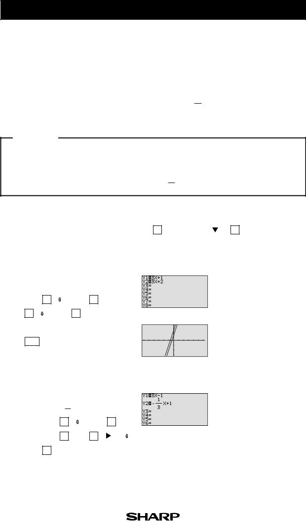
A linear equation of y in terms of x can be expressed by the slope-intercept form y = mx+b, where m is the slope and b is the y - intercept. We call this equation a linear equation since its graph is a straight line. Equations where the exponents on the x and y are 1 (implied) are considered linear equations. In graphing linear equations on the calculator, we will let the x variable be represented by the horizontal axis and let y be represented by the vertical axis.

Example

Draw graphs of two equations by changing the slope or the y- intercept.

1. Graph the equations y = x and y = 2x.

2. Graph the equations y = x and y = 12 x.

3. Graph the equations y = x and y = - x.

4. Graph the equations y = x and y = x + 2.

Before There may be differences in the results of calculations and graph plotting depending on the setting. Starting Return all settings to the default value and delete all data.

Step & Key Operation	Display	Notes
(When using EL-9650/9600c)	(When using EL-9650/9600c)
*Use either pen touch or cursor to operate.

1-1 Enter the equation y = x for Y1 and y = 2x for Y2.

Y= X//T/n ENTER * 2 X//T/n

1-2 View both graphs.

GRAPH

2-1

Enter the equation y =

1

x for Y2.

2

Y=

*

CL

1

a

/b

2

n

*

X/ /T/

2-2

View both graphs.

GRAPH

The equation Y1 = x is displayed first, followed by the equation Y2 = 2x. Notice how Y2 becomes steeper or climbs faster. Increase the size of the slope (m>1) to make the line steeper.

Notice how Y2 becomes less steep or climbs slower. Decrease the size of the slope (0<m<1) to make the line less steep.

1-1

EL-9650/9600c/9450/9400 Graphing Calculator

3-1

3-2

Step & Key Operation	Display	Notes
(When using EL-9650/9600c)	(When using EL-9650/9600c)
*Use either pen touch or cursor to operate.

Enter the equation y = - x for Y2.

Y= * CL (-) X//T/n

View both graphs.

GRAPH

Notice how Y2 decreases (going down from left to right) instead of increasing (going up from left to right). Negative slopes (m<0) make the line decrease or go down from left to right.

4-1		Enter the equation y = x + 2 for
		Y2.
		Y=			*	CL		X/ /T/n		+	2
4-2											Adding 2 will shift the y = x
	View both graphs.
											graph upwards.
		GRAPH

Making a graph is easy, and quick comparison of several graphs will help students understand the characteristics of linear equations.

1-1

EL-9650/9600c/9450/9400 Graphing Calculator

Parallel and Perpendicular Lines

Parallel and perpendicular lines can be drawn by changing the slope of the linear equation and the y intercept. A linear equation of y in terms of x can be expressed by the slopeintercept form y = mx + b, where m is the slope and b is the y-intercept.

Parallel lines have an equal slope with different y-intercepts. Perpendicular lines have slopes that are negative reciprocals of each other (m = - m1 ). These characteristics can be verified by graphing these lines.

Example

Graph parallel lines and perpendicular lines.

1. Graph the equations y = 3x + 1 and y = 3x + 2.

2. Graph the equations y = 3x - 1 and y = - 31 x + 1.

Before	There may be differences in the results of calculations and graph plotting depending on the setting.
Starting Return all settings to the default value and delete all data.
	Set the zoom to the decimal window:	ZOOM		C	* (	ENTER		ALPHA			* ) 7 *
Step & Key Operation				Display							Notes
	(When using EL-9650/9600c)	(When using EL-9650/9600c)
*Use either pen touch or cursor to operate.

1-1

1-2

2-1

Enter the equations y = 3x + 1 for Y1 and y = 3x + 2 for Y2.

Y=		3		X/ /T/n		+	1	ENTER	*
3	X/ /T/n			+	2

View the graphs.

GRAPH

Enter the equations y = 3x - 1 for Y1 and y = - 31 x + 1 for Y2.

Y=		CL	3	X/ /T/n		—		1			ENTER		*
CL		(-)	1	a/b	3				*		X/ /T/n
+	1

These lines have an equal slope but different y-intercepts. They are called parallel, and will not intersect.

1-2

EL-9650/9600c/9450/9400 Graphing Calculator

Step & Key Operation	Display	Notes
(When using EL-9650/9600c)	(When using EL-9650/9600c)
*Use either pen touch or cursor to operate.

2-2 View the graphs.

GRAPH

These lines have slopes that are negative reciprocals of each other (m = - m1 ). They are called perpendicular. Note that these intersecting lines form four equal angles.

The Graphing Calculators can be used to draw parallel or perpendicular lines while learning the slope or y -intercept of linear equations.

1-2

EL-9650/9600c Graphing Calculator

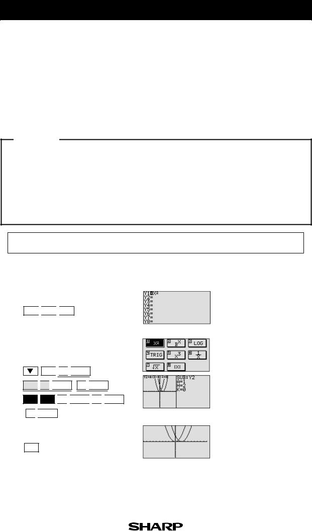
Slope and Intercept of Quadratic Equations

A quadratic equation of y in terms of x can be expressed by the standard form y = a (x - h) 2+ k, where a is the coefficient of the second degree term (y = ax 2 + bx + c) and (h, k) is the vertex of the parabola formed by the quadratic equation. An equation where the largest exponent on the independent variable x is 2 is considered a quadratic equation. In graphing quadratic equations on the calculator, let the x-variable be represented by the horizontal axis and let y be represented by the vertical axis. The graph can be adjusted by varying the coefficients a, h, and k.

Example

Graph various quadratic equations and check the relation between the graphs and the values of coefficients of the equations.

1. Graph y = x 2

2. Graph y = x 2

3. Graph y = x 2

4. Graph y = x 2

and y = (x - 2) 2. and y = x 2 + 2. and y = 2x 2. and y = - 2x 2.

Before There may be differences in the results of calculations and graph plotting depending on the setting. Starting Return all settings to the default value and delete all data.

Step & Key Operation Display Notes

*Use either pen touch or cursor to operate.

1-1 Enter the equation y = x 2 for Y1.

Y= X//T/n x2

1-2 Enter the equation y = (x - 2) 2 for Y2 using Sub feature.

EZ 1 ENTER *

ALPHA C ENTER * 1 ENTER *

2nd F SUB 1 ENTER 2 ENTER

( 0 ENTER )

1-3 View both graphs.

GRAPH

Notice that the addition of -2 within the quadratic operation moves the basic y = x 2 graph right two units (adding 2 moves it left two units) on the x-axis.

This shows that placing an h (>0) within the standard form y = a (x - h) 2 + k will move the basic graph right h units and placing an h (<0) will move it left h units on the x-axis.

2-1

EL-9650/9600c Graphing Calculator

Step & Key Operation

Display

Notes

*Use either pen touch or cursor to operate.

2-1 Change the equation in Y2 to y = x 2+2.

Y=			*	2nd F		SUB			0

ENTER 2 ENTER

2-2 View both graphs.

GRAPH

Notice that the addition of 2 moves the basic y = x 2 graph up two units and the addition of - 2 moves the basic graph down two units on the y-axis. This demonstrates the

fact that adding k (>0) within the standard form y = a (x - h) 2 + k will move the basic graph up k units and placing k (<0) will move the basic graph down k units on the y-axis.

3-1 Change the equation in Y2 to y = 2x 2.

Y=				*	2nd F			SUB	2	ENTER
	0
			ENTER

3-2 View both graphs.

GRAPH

Notice that the multiplication of 2 pinches or closes the basic y = x 2 graph. This demonstrates the fact that multiplying an a (> 1) in the standard form y = a (x - h) 2 + k will pinch or close the basic graph.

4-1

4-2

Change the equation in Y2 to y = - 2x 2.

Y=								(	)	2
			*	2nd F		SUB		-

ENTER

View both graphs.

GRAPH

Notice that the multiplication of -2 pinches or closes the basic y =x 2 graph and flips it (reflects it) across the x-axis. This demonstrates the fact that multiply-

ing an a (<-1) in the standard form y = a (x - h) 2 + k will pinch or close the basic graph and flip it (reflect it) across the x-axis.

The EL-9650/9600c allows various quadratic equations to be graphed easily. Also the characteristics of quadratic equations can be visually shown through the relationship between the changes of coefficient values and their graphs, using the Substitution feature.

2-1

EL-9650/9600c/9450/9400 Graphing Calculator

Shifting a Graph of Quadratic Equations

A quadratic equation of y in terms of x can be expressed by the standard form y = a (x - h) 2 + k, where a is the coefficient of the second degree term (y = ax 2 + bx + c) and (h, k) is the vertex of the parabola formed by the quadratic equation. An equation where the largest exponent on the independent variable x is 2 is considered a quadratic equation. In graphing quadratic equations on the calculator, let the x-variable be represented by the horizontal axis and let y be represented by the vertical axis. The relation of an equation and its graph can be seen by moving the graph and checking the coefficients of the equation.

Example

Move or pinch a graph of quadratic equation y = x 2 to verify the relation between the coefficients of the equation and the graph.

1. Shift the graph y = x 2 upward by 2.

2. Shift the graph y = x 2 to the right by 3.

3. Pinch the slope of the graph y = x 2.

Before There may be differences in the results of calculations and graph plotting depending on the setting. Starting Return all settings to the default value and delete all data.

Step & Key Operation	Display	Notes
(When using EL-9650/9600c)	(When using EL-9650/9600c)
*Use either pen touch or cursor to operate.

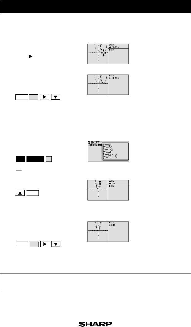
1-1 Access Shift feature and select the equation y = x 2.

2nd F SHIFT/CHANGE A *

1 *

1-2 Move the graph y = x 2 upward by 2.

ENTER *

1-3 Save the new graph and observe the changes in the graph and the equation.

ENTER ALPHA

Notice that upward movement of the basic y = x 2 graph by 2 units in the direction of the y- axis means addition of 2 to the y-intercept. This demonstrates

that upward movement of the graph by k units means adding a k (>0) in the standard form y = a (x - h) 2 + k.

2-2

EL-9650/9600c/9450/9400 Graphing Calculator

Step & Key Operation	Display	Notes
(When using EL-9650/9600c)	(When using EL-9650/9600c)
*Use either pen touch or cursor to operate.

2-1 Move the graph y = x 2 to the right by 3.

CL				(three times)	ENTER		*

2-2 Save the new graph and observe the changes in the graph and the equation

ENTER ALPHA

Notice that movement of the basic y = x2 graph to the right by 3 units in the direction of the x-axis is equivalent to the addition of 3 to the x -intercept.

This demonstrates that movement of the graph to the right means adding an h (>0) in the standard form y = a (x - h) 2 + k and movement to the left means subtracting an h (<0).

3-1 Access Change feature and select the equation y = x 2.

2nd F SHIFT/CHANGE B *

1 *

3-2 Pinch the slope of the graph.

ENTER

3-3 Save the new graph and observe the changes in the graph and the equation.

ENTER ALPHA

Notice that pinching or closing the basic y = x 2 graph is equivalent to increasing an a (>1) within the standard form y = a (x - h) 2 + k and broadening the graph is equivalent to decreasing an a (<1).

The Shift/Change feature of the EL-9650/9600c/9450/9400 allows visual understanding of how graph changes affect the form of quadratic equations.

2-2

EL-9650/9600c Graphing Calculator

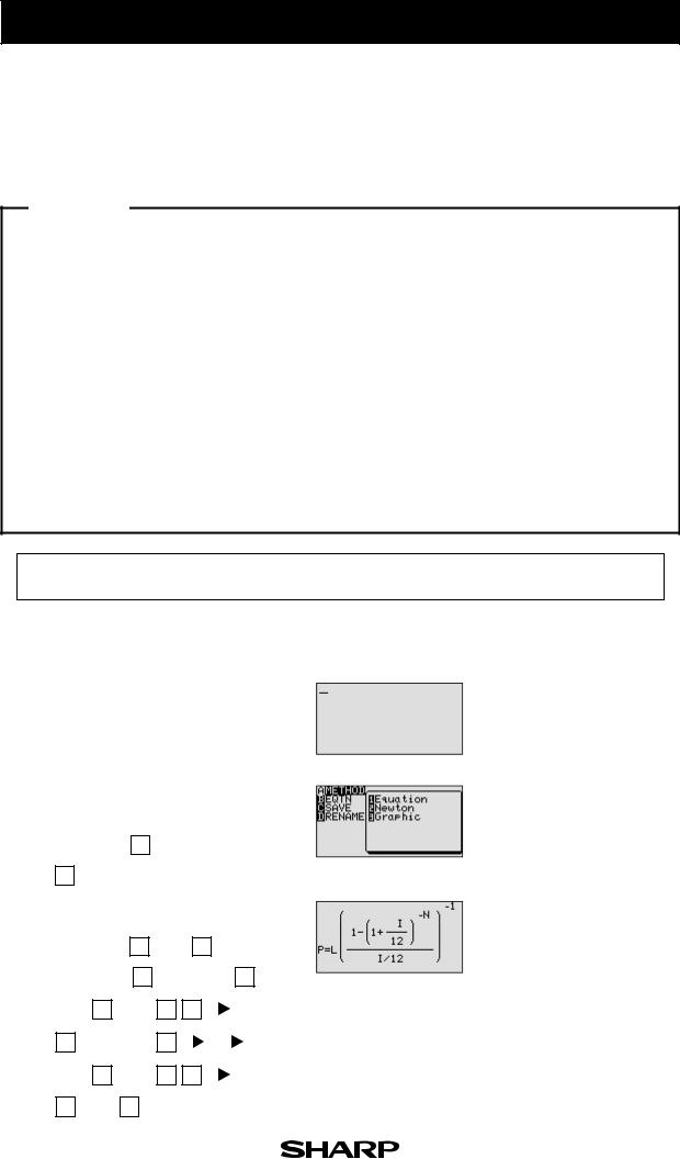
Solving a Literal Equation Using the Equation Method (Amortization)

The Solver mode is used to solve one unknown variable by inputting known variables, by three methods: Equation, Newton’s, and Graphic. The Equation method is used when an exact solution can be found by simple substitution.

Example

Solve an amortization formula. The solution from various values for known variables can be easily found by giving values to the known variables using the Equation method in the Solver mode.

						I				-1
							-N
		1-(1+					)			P= monthly payment	I= interest rate
	The formula : P = L				12
										L= loan amount	N=number of months
				I / 12

1. Find the monthly payment on a $15,000 car loan, made at 9% interest over four

years (48 months) using the Equation method.

2. Save the formula as “AMORT”.

3. Find amount of loan possible at 7% interest over 60 months with a $300

payment, using the saved formula.

Before There may be differences in the results of calculations and graph plotting depending on the setting. Starting Return all settings to the default value and delete all data.

Step & Key Operation

Display

Notes

*Use either pen touch or cursor to operate.

1-1 Access the Solver feature.							This screen will appear a few
							seconds after “SOLVER” is dis-
	2nd F		SOLVER				played.
1-2 Select the Equation method for
solving.
	2nd F		SOLVER		A	*

1 *

1-3 Enter the amortization formula.

2nd F				SOLVER				P		=					L					ALPHA
																						1
	(			a/b			1			—						(											+
ALPHA				1		a/b				1			2										*		)
ab		(		)		ALPHA				N
			-																							*
ALPHA				I						1			2										*		)
a	b		(	)		1
				-

3-1

EL-9650/9600c Graphing Calculator

Step & Key Operation

Display

Notes

*Use either pen touch or cursor to operate.

1-4 Enter the values L=15,000, I=0.09, N=48.

ENTER					*	1	5 0 0			0
					0	9				4
ENTER		* •						ENTER	*
8	ENTER

1-5 Solve for the payment(P).

* 2nd F EXE

( CL )

2-1 Save this formula.

2nd F SOLVER C * ENTER *

2-2 Give the formula the name AMORT.

A M O R T ENTER

3-1 Recall the amortization formula.

2nd F SOLVER B *

0 1 *

3-2 Enter the values: P = 300, I = 0.01, N = 60

ENTER 3 0 0 ENTER 0 ENTER *

• 0 1 ENTER * 6 1 ENTER

3-3 Solve for the loan (L).

* 2nd F EXE

The monthly payment (P) is $373.28.

The amount of loan (L) is $17550.28.

With the Equation Editor, the EL-9650/9600c displays equations, even complicated ones, as they appear in the textbook in easy to understand format. Also it is easy to find the solution for unknown variables by recalling a stored equation and giving values to the known variables in the Solver mode when using the EL-9650/9600c.

3-1

EL-9650/9600c Graphing Calculator

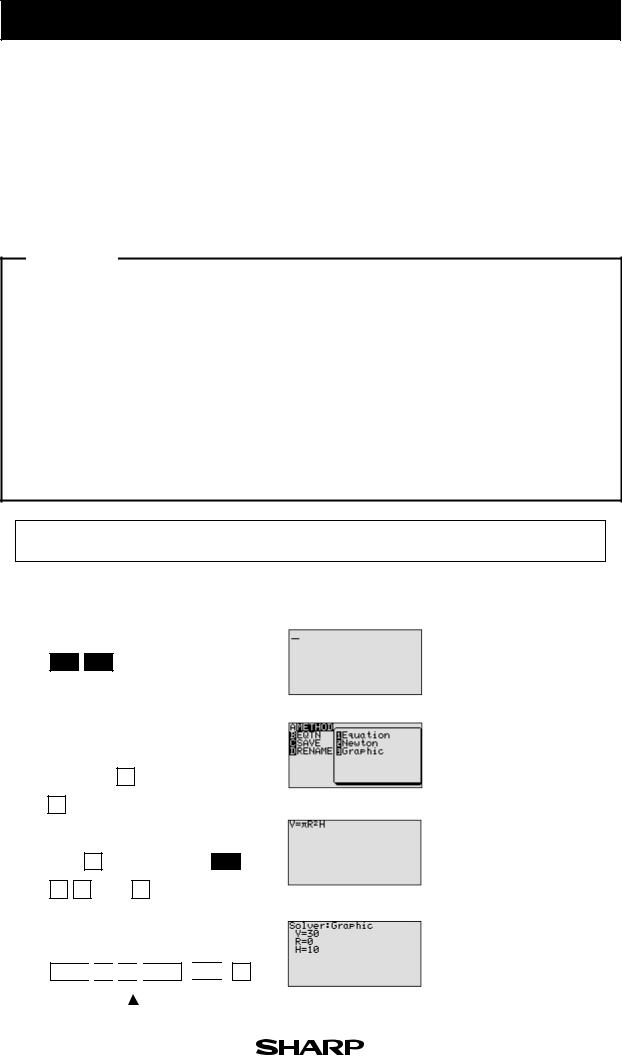
Solving a Literal Equation Using the Graphic Method (Volume of a Cylinder)

The Solver mode is used to solve one unknown variable by inputting known variables. There are three methods: Equation, Newton’s, and Graphic. The Equation method is used when an exact solution can be found by simple substitution. Newton’s method implements an iterative approach to find the solution once a starting point is given. When a starting point is unavailable or multiple solutions are expected, use the Graphic method. This method plots the left and right sides of the equation and then locates the intersection(s).

Example

Use the Graphic method to find the radius of a cylinder giving the range of the unknown variable.

The formula : V = π r 2h ( V = volume r = radius h = height)

1. Find the radius of a cylinder with a volume of 30in3 and a height of 10in, using the Graphic method.

2. Save the formula as “V CYL”.

3. Find the radius of a cylinder with a volume of 200in 3 and a height of 15in, using the saved formula.

Before There may be differences in the results of calculations and graph plotting depending on the setting. Starting Return all settings to the default value and delete all data.

1-1

1-2

1-3

1-4

Step & Key Operation

Display

Notes

*Use either pen touch or cursor to operate.

Access the Solver feature.

2nd F SOLVER

Select the Graphic method for solving.

2nd F

SOLVER

A

*

3 *

Enter the formula V = π r 2h.

π

ALPHA

V

ALPHA

=

2nd F

ALPHA

R

x 2

ALPHA

H

This screen will appear a few seconds after “SOLVER” is displayed.

Enter the values: V = 30, H = 10. Solve for the radius (R).

ENTER 3 0 ENTER * * 1

0		ENTER			*	2nd F		EXE

3-2

EL-9650/9600c Graphing Calculator

Step & Key Operation

Display

Notes

*Use either pen touch or cursor to operate.

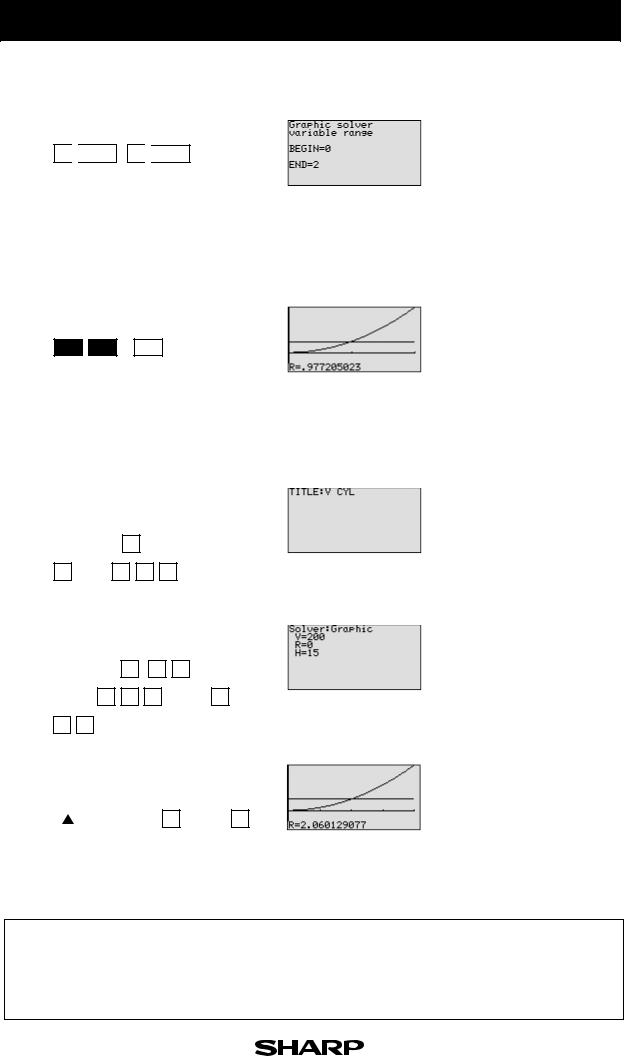
1-5 Set the variable range from 0 to 2.

0 ENTER * 2 ENTER

The graphic solver will prompt with a variable range for solving.

r 2 =	30	=	3	<3
	10π		π

r =1 r 2 = 12 = 1 <3 r =2 r 2 = 22 = 4 >3

1-6 Solve.

2nd F EXE ( CL )

Use the larger of the values to be safe.

The solver feature will graph the left side of the equation (volume, y = 30), then the right side of the equation (y = 10r 2), and finally will calculate the intersection of the two graphs to find the solution.

The radius is 0.98 in.

2

Save this formula.

Give the formula the name “V CYL”.

2nd F

SOLVER

C

*

ENTER

*

V

SPACE

C

Y

L

ENTER

3-1

Recall the formula.

Enter the values: V = 200, H = 15.

2nd F

SOLVER

B

*

0

1

*

0

0

0

ENTER

2

ENTER

ENTER

1

5

ENTER

3-2

Solve the radius setting the variable

range from 0 to 4.

*

2nd F

EXE

0

ENTER

4

ENTER

2nd F

EXE

	200		14
r 2 =			= π < 14
		15π
r	= 3 r 2 = 32 = 9 < 14
r	= 4 r 2 = 42 = 16 > 14

Use 4, the larger of the values, to be safe.

The answer is : r = 2.06

One very useful feature of the calculator is its ability to store and recall equations. The solution from various values for known variables can be easily obtained by recalling an equation which has been stored and giving values to the known variables. The Graphic method gives a visual solution by drawing a graph.

3-2

EL-9650/9600c Graphing Calculator

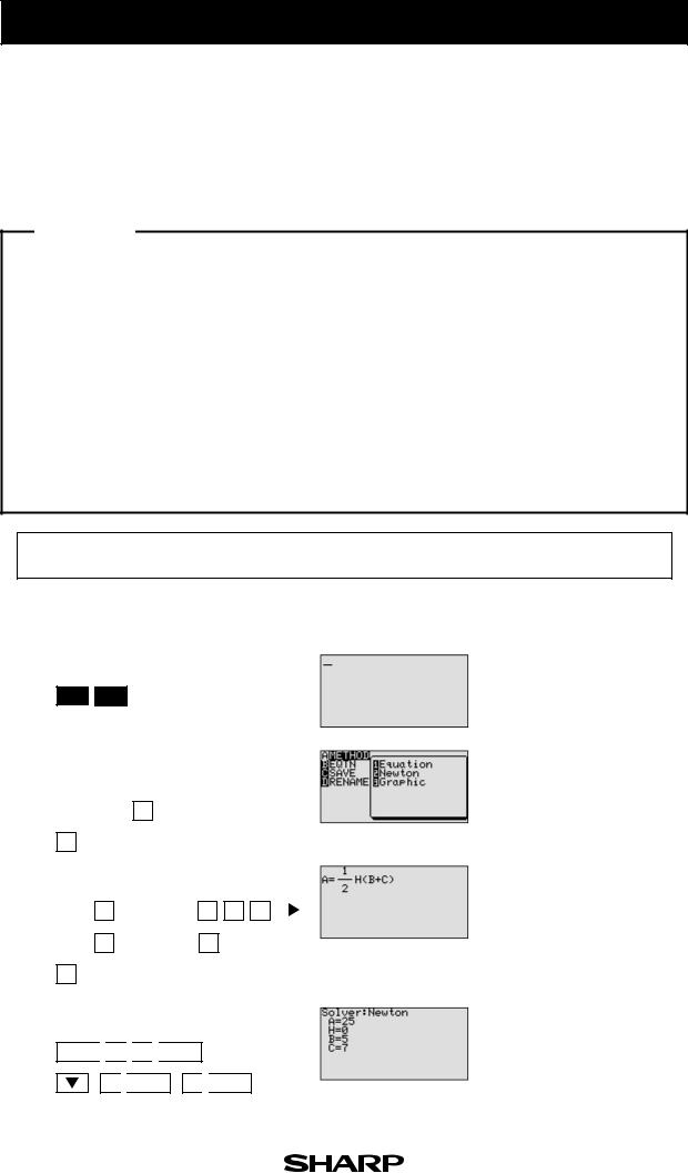
Solving a Literal Equation Using Newton's Method(Area of a Trapezoid)

The Solver mode is used to solve one unknown variable by inputting known variables. There are three methods: Equation, Newton’s, and Graphic. The Newton’s method can be used for more complicated equations. This method implements an iterative approach to find the solution once a starting point is given.

Example

Find the height of a trapezoid from the formula for calculating the area of a trapezoid using Newton’s method.

	The formula : A=	1	h(b+c)	(A = area h = height b = top face c = bottom face)
		2

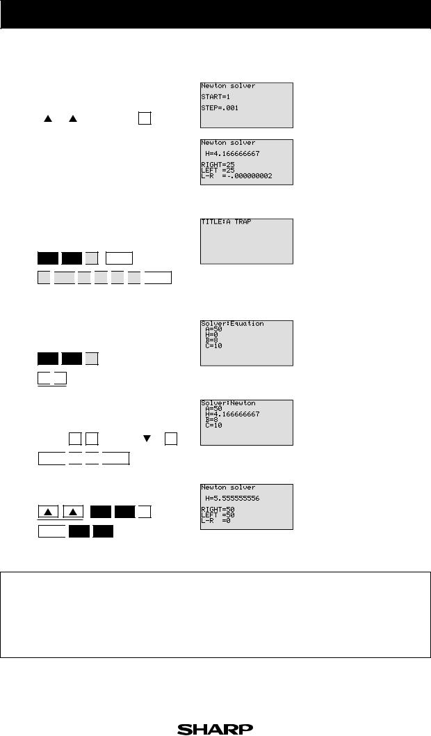
1. Find the height of a trapezoid with an area of 25in2 and bases of length 5in and 7in using Newton's method. (Set the starting point to 1.)

2. Save the formula as “A TRAP”.

3. Find the height of a trapezoid with an area of 50in2 with bases of 8in and 10in using the saved formula. (Set the starting point to 1.)

Before There may be differences in the results of calculations and graph plotting depending on the setting. Starting Return all settings to the default value and delete all data.

Step & Key Operation Display Notes

*Use either pen touch or cursor to operate.

1-1 Access the Solver feature.

2nd F SOLVER

This screen will appear a few seconds after “SOLVER” is displayed.

1-2

Select Newton's method

for solving.

2nd F

SOLVER

A

*

1-3

2 *

1

Enter the formula A =

h(b+c).

2

a/b

2

ALPHA

A

ALPHA

=

1

*

ALPHA

H

(

ALPHA

B

+

ALPHA

C

)

1-4 Enter the values: A = 25, B = 5, C = 7

ENTER 2 5 ENTER *

* 5 ENTER * 7 ENTER

3-3

EL-9650/9600c Graphing Calculator

Step & Key Operation

Display

Notes

*Use either pen touch or cursor to operate.

1-5 Solve for the height and enter a starting point of 1.

*

2nd F

EXE

1

ENTER

1-6 Solve.

(

)

2nd F

EXE

CL

2 Save this formula. Give the formula the name “A TRAP”.

2nd F SOLVER C * ENTER

A SPACE T R A P ENTER

3-1 Recall the formula for calculating the area of a trapezoid.

2nd F SOLVER B *

0 1

3-2 Enter the values:

A = 50, B = 8, C = 10.

ENTER	5 0	ENTER	*		* 8

ENTER 1 0 ENTER

3-3 Solve.

* 2nd F EXE 1

ENTER 2nd F EXE

Newton's method will prompt with a guess or a starting point.

The answer is : h = 4.17

The answer is : h = 5.56

One very useful feature of the calculator is its ability to store and recall equations. The solution from various values for known variables can be easily obtained by recalling an equation which has been stored and giving values to the known variables in the Solver mode. If a starting point is known, Newton's method is useful for quick solution of a complicated equation.

3-3