

Page 1

i
Contents
Servotest
DFG
Desired File Generator
Revision number Date Author Description
1 9/10/00 SLB Created
2 29/03/01 VB Added PSD and Shock sections
3 19/05/01 VB Added sweep section
4 13/09/01 JM Added Crest Factor and notes on editing sweep
5
7
8
22/07/02
9/03/04
10/04/13
11/05/15
PFW
JM
JGW
JGW
“Ltd” dropped
Added Import from EXCEL
Added ZPA Compression and envelope for FRS
Added Freq OP sweep and Margins for RRS
Page 2

ii
Contents
Contents
Servotest .................................................................................................................................... 1
DFG ........................................................................................................................................... 1
Desired File Generator ............................................................................................................ 1
Contents ..................................................................................................................................... i
Introduction .............................................................................................................................. 1
Using FRS Editor ..................................................................................................................... 2
Getting Started ........................................................................................................................ 1
The Main Application Window .............................................................................................. 1
Repeating the search ...................................................................................................................................... 2
Increasing the minimum frequency of interest ................................................................................................ 2
Plot RRS ......................................................................................................................................................... 2
Generate .......................................................................................................................................................... 4
Global settings ........................................................................................................................ 5
Save Time History .................................................................................................................. 7
RRS Profile Files .................................................................................................................... 7
New Profile ..................................................................................................................................................... 7
Saving the profile ............................................................................................................................................ 7
Loading the profile ......................................................................................................................................... 8
Importing Data from MS EXCEL ................................................................................................................... 8
Using PSD Editor ..................................................................................................................... 9
Getting Started ........................................................................................................................ 9
The Main Application Window .............................................................................................. 9
Plot PSD ....................................................................................................................................................... 10
Generate ................................................................................................................................ 11
Global Settings ..................................................................................................................... 12
Save Time History ................................................................................................................ 14
PSD Profile Files .................................................................................................................. 14
New Profile ................................................................................................................................................... 14
Saving the profile .......................................................................................................................................... 14
Loading the profile ....................................................................................................................................... 15
Using Shock Editor ................................................................................................................ 16
Getting Started ...................................................................................................................... 16
The Main Application Window ............................................................................................ 16
Generate ................................................................................................................................ 17
Global Settings ..................................................................................................................... 19
Constraints ............................................................................................................................ 19
Output File Setup .................................................................................................................. 20
Save Time History ................................................................................................................ 20
Shock Profile Files ................................................................................................................ 21
New Profile ................................................................................................................................................... 21
Saving the profile .......................................................................................................................................... 21
Loading the profile ....................................................................................................................................... 21
Page 3

Using Sweep generator .......................................................................................................... 22
Getting Started ...................................................................................................................... 22
The Main Application Window ............................................................................................ 22
Global Settings ..................................................................................................................... 23
Generate ................................................................................................................................ 24
Save Time History ................................................................................................................ 25
Sweep Profile Files ............................................................................................................... 26
New Profile ................................................................................................................................................... 26
Saving the profile .......................................................................................................................................... 26
Loading the profile ....................................................................................................................................... 26
Appendix A Edit Menu Options ........................................................................................... 27
Appendix B Excel Spreadsheet Format for Importing to DFG ......................................... 28
Appendix C Contacting Servotest ........................................................................................ 29
11
Page 4

Page 5
1
Introduction
Desired File Generator is a program that allows the user to generate
Servotest binary files (.sbf or .sef) containing time histories that meet
certain frequency or time domain criteria. The four types of
specification supported are :
1. Power Spectral Densities
2. Frequency response Spectra
3. Classical shock pulses
4. Sinusoidal frequency sweeps
These specifications are entered via four different editors (PSD, FRS,
Shock and Sweep) and time histories meeting them are generated,
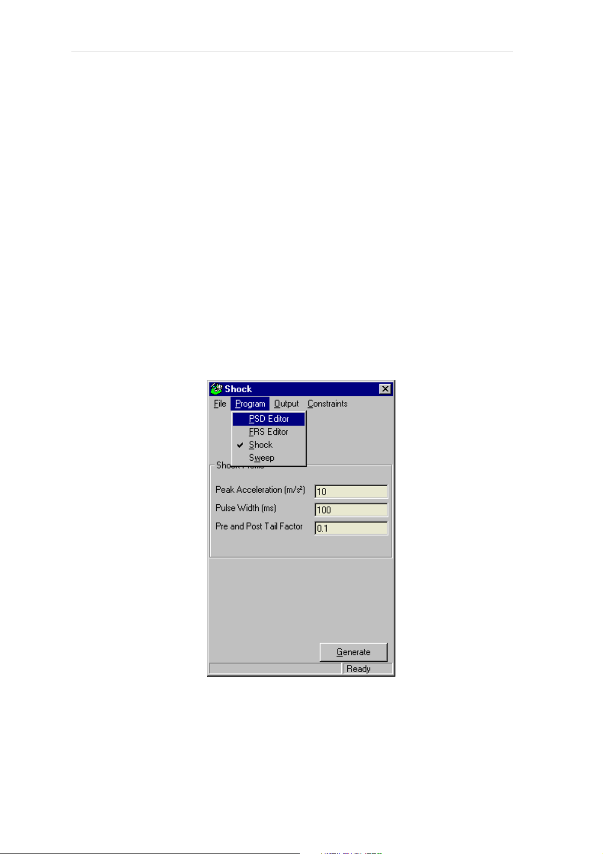
plotted and saved to disk. Switching from one editor to another is
done via the Program menu as shown in Figure 1.
Introduction
Figure 1: Switching from one editor to another
This manual describes the use of each program sequentially.
Page 6

2
Using FRS Editor
Frequency Response Spectra (FRS) are widely used in earthquake
engineering to evaluate the energy content of acceleration time
histories. Calculating an FRS from a time history is straight forward
and is done by many frequency domain analysis programs such as
Servotest’s Data Analysis Package (DAP). However, the reverse
operation that consists of generating a random acceleration time
history based on a Required Response Spectrum (RRS) is not a
straightforward matter and can be very time consuming.
One technique consists of combining a large number of wavelets of
various frequencies and amplitudes to produce an adequate time
history. However, the criticism that is often made is that the energy of
such a signal is not equally spread over the whole duration of the time
history.
Servotest’s FRS Editor uses another technique that is based on a
white noise signal that is shaped in the frequency domain (using
FFTs) in order to fit the specified RRS.
Introduction
In the case of multiple channel FRS, the corresponding time histories
generated are uncorrelated.
Page 7
Getting Started
After installing DFG a shortcut will have been placed on your desktop
which can be used to run the program. Select the FRS Editor as
shown in Figure 1.
The Main Application Window
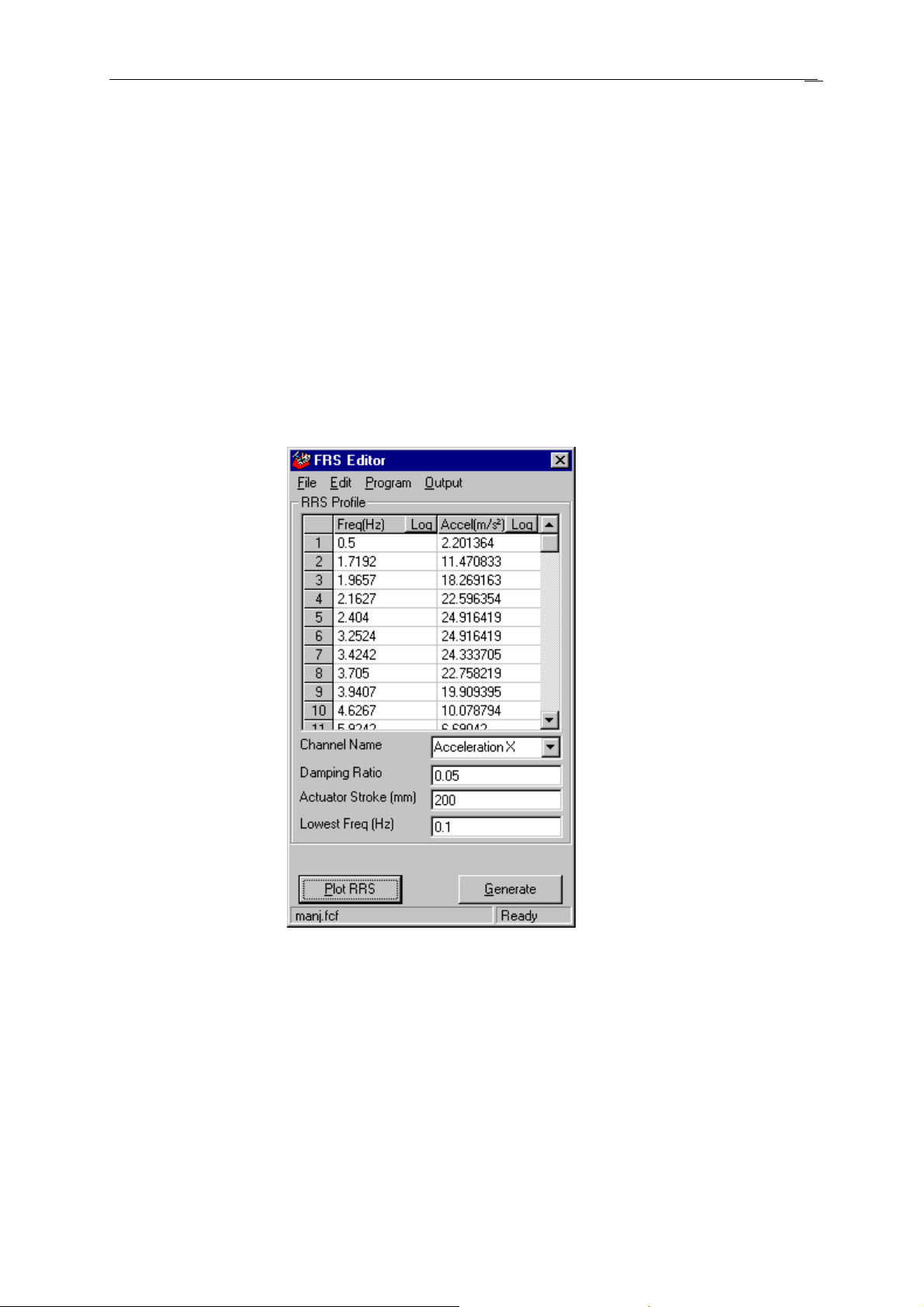
The main application window is used to enter the information
regarding the Required Response Spectrum (RRS) profile.
1
Figure 2: FRS Editor main window
FRS Editor loads the last saved RRS profile on starting. If this is the
first time FRS Editor has been used or no profiles have been saved
then fixed default values are loaded into the working RRS profile.
If any of the fields listed below are left empty or are invalid then these
fixed default values will be used instead.
• Frequency and Acceleration Table. Use this table to enter the
2
frequency in Hertz and the acceleration in m/s
.
Page 8
Figure
• Channel Name. Up to 20 characters are allowed. In the case of
multiple channels, use the combo box to switch to another
channel.
• Damping Ratio. The damping ratio must be a value greater
than zero and less than or equal to one. Its default value is 0.02.
• Actuator stroke. Maximum peak displacement allowed by the
system (in mm).
• Lowest Frequency. Lowest frequency of interest (in Hz). It is
the frequency below which the FRS of the acceleration time
history is allowed to lie below the RRS.
The lowest frequency of interest should be at least the lowest
frequency specified in the RRS. If it is set too low, the
displacement signal produced may exceed the maximum peak to
peak displacement allowed by the system. In this case, the user is
warned by an indication of the actual peaks of the displacement,
and the file should not be played to the rig. The two possible
courses of action are presented next.
2
Repeating the search
If the Random Number Seed in the Global Settings panel is set to ‘0’
(see Global Settings), a totally new random time history is generated
each time the Generate command is used. In particular, its peak to
peak amplitude is different to that of the previous one.
So whenever the peak to peak amplitude of the displacement exceeds
the maximum allowed by less than say 50%, it is worth trying again
by pressing the Generate button.
Increasing the minimum frequency of interest
If the previous solution consistently fails or if the peak to peak
amplitude of the displacement exceeds the maximum allowed by a
large amount, the only solution is to increase the minimum frequency
of interest. The RRS will then be ignored below this new frequency
and the slow motions that are responsible for large excursions will be
removed.
Plot RRS
The Plot RRS button is only enabled once data has
been entered in the current RRS profile or after a
valid profile file has been loaded.
3: Plot RRS button
Page 9
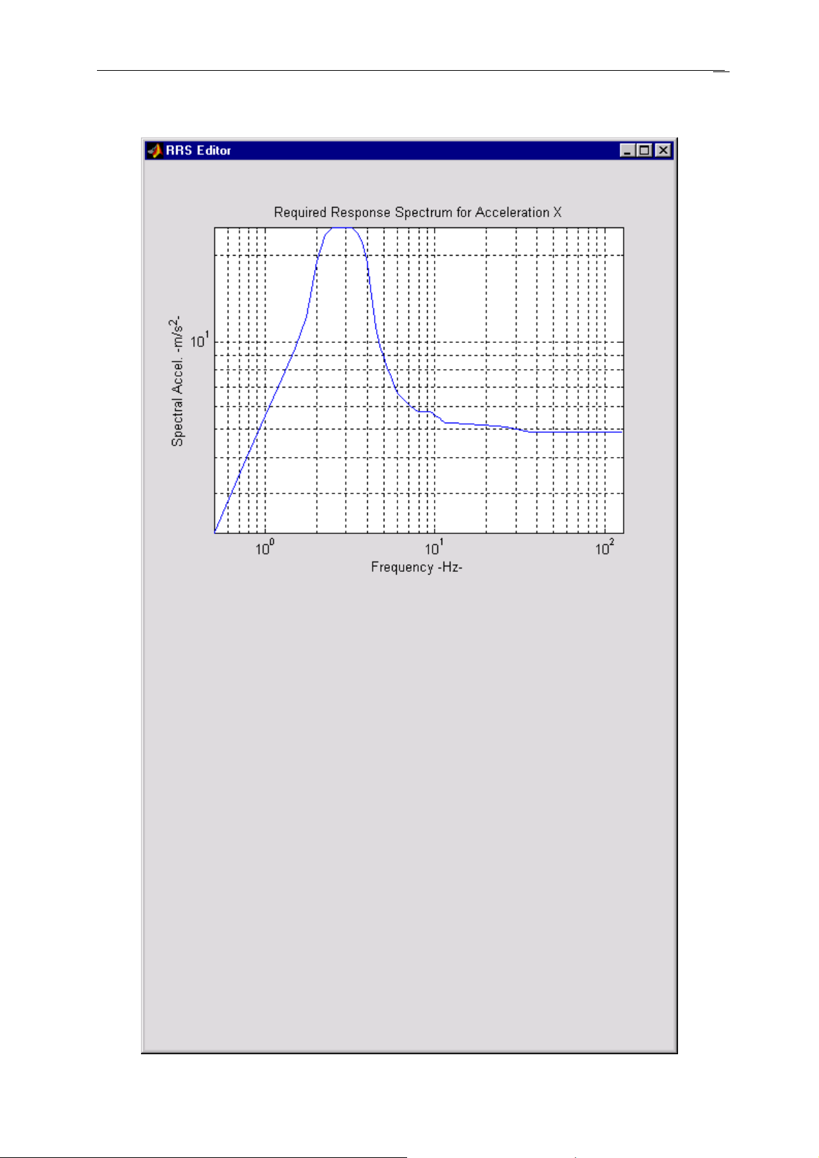
Selecting the Plot RRS button will open a window containing a plot
of the user entered RRS profile.
3
Page 10

Figure 4: RRS plot
This window can be left open while the user makes changes to the
profile on the main menu but the Plot RRS button must be pushed
again to redraw any new values entered.
Generate
The Generate button is only enabled once the Plot RRS button has
been selected.
Selecting the Generate button opens a new window containing the
time domain plots. This window may take a few seconds to appear
depending upon the number of RRS profiles and their complexity.
On pushing the Generate button the status bar at the bottom of the
main application window will change from “Ready” to
“Processing…” indicating that this command is in process and no
further changes to the profile can be made until this command has
been completed.
4
Page 11
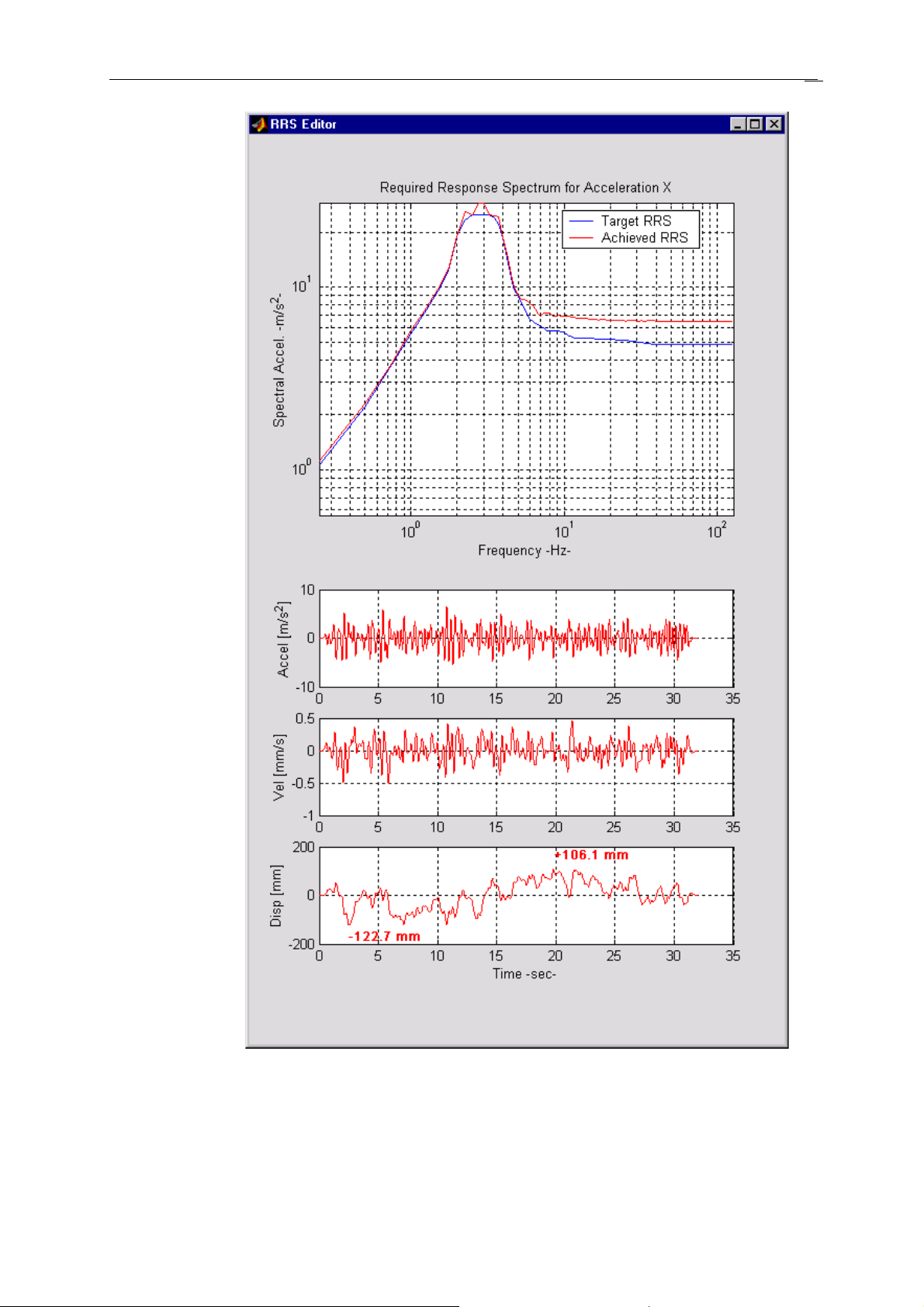
Figure
5
5: Target and achieved RRS and corresponding time history
Page 12
Global settings
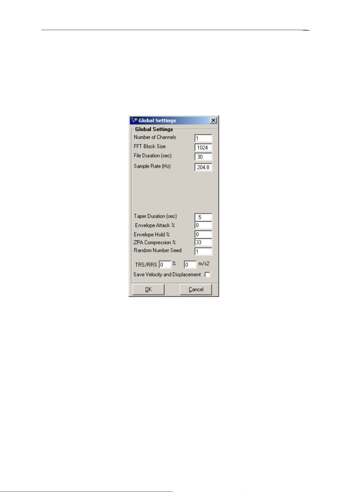
The Output menu contains an element called Global Settings.
Selecting this opens a window (see Figure 6) that allows the user to
set some parameters that are valid for all the channels defined in the
main window. These settings must be selected before the time
histories are generated.
6
Figure 6: The Global Settings
• Number of channels. This specifies the number of RRS
profiles that will be defined and therefore the number of
uncorrelated acceleration waveforms generated.
• FFT Block Size. Values entered in the FFT Block Size edit box
will be rounded to the nearest power of two. A default value of
512 is used if no value is entered. Note that the FRS’s spectral
resolution is given by the ratio: Sample Rate / FFT Block Size.
• File Duration in seconds. It has a default value of 20s.
• Sample Rate in Hertz. This value must be greater than twice
the highest frequency of interest and will default to a value of
102.4Hz.
Page 13
10010110
15
H
old Attack
0%
33%
RRS
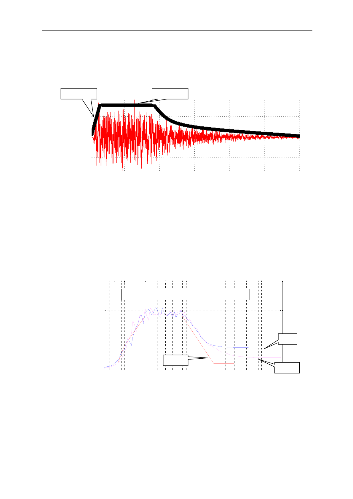
Typical effects of ZPA Compression
• Taper Duration in seconds. It has a default value of 3s.
• Envelope Attack and Hold in % (percent) - can be used to
generate a response shape looking more like a real earthquake.
If Hold is 0% (default) then this additional shaping is not applied.
The Taper defined by Taper parameter is always active in
addition to the envelope shaping.
7
10
• ZPA Compression in %. When a shaped RRS is defined it is
common that so much energy is required in the low frequencies
that peak acceleration must significantly exceed the specified
zero period acceleration. Application of compression can be
beneficial in reducing ZPA – typical optimum is 33% . If the
compression is 0% (default) no compression is applied. Values
greater than 90% have negligible effect.
5
0
2
• Random Number Seed. This integer value is used by the
random number generator. A value of ‘0’ generates a unique
sequence of random numbers each time the ‘Generate’ button is
pressed whereas numbers other than zero generate the same
random sequence unique to that Seed Number.
Page 14
• Save Velocity and Displacement. If this box is left unticked,
only the acceleration channels will be saved to disk. If it is ticked,
the corresponding velocity and displacement waveforms will also
be saved.
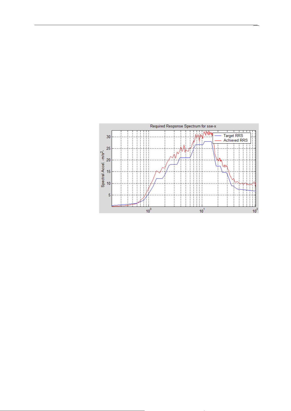
• TRS/RRS . When generating target time histories it is a
common requirement for a test response spectrum that exceeds
the specified RRS ( required response spectrum). An entry in
the TRS/RRS % will increase the generated FRS by the specified
percentage (e.g. 5%). An entry in the field TRS/RRS m/s2 will
add a fixed additional level to the required amplitude (e.g. 1 m/s2)
The percentage increase is applied first
8
Page 15
Figure
Save Time History
9
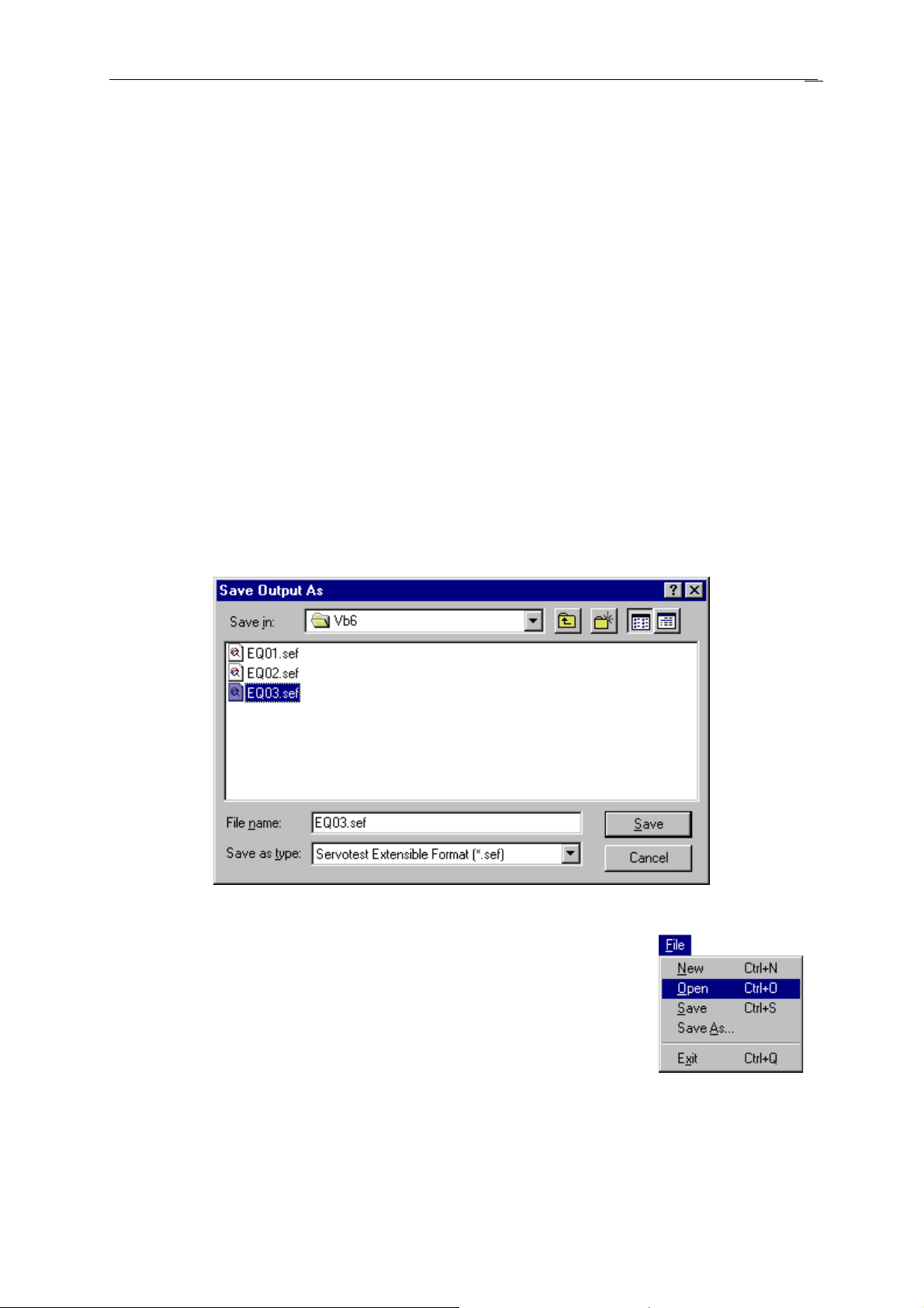
Once the time histories have been generated, they can be saved on
disk by selecting Output | Save Time History and selecting an sbf or
sef file name.
RRS Profile Files
RRS profile files are a means by which the
profile data can be stored for retrieval.
Figure 7: Saving the time histories
On start up FRS Editor will always load the last
RRS profile saved.
8: File Menu
Page 16
Figure
New Profile
Selecting File | New clears the frequency and acceleration table
and loads the default values into the other fields ready for a new
profile to be entered.
Saving the profile
Selecting File | Save will prompt the user for a filename if no
profile file is being used, otherwise it will save any changes.
Selecting File | Save As will prompt the user for a filename
and save the current RRS profile under that filename.
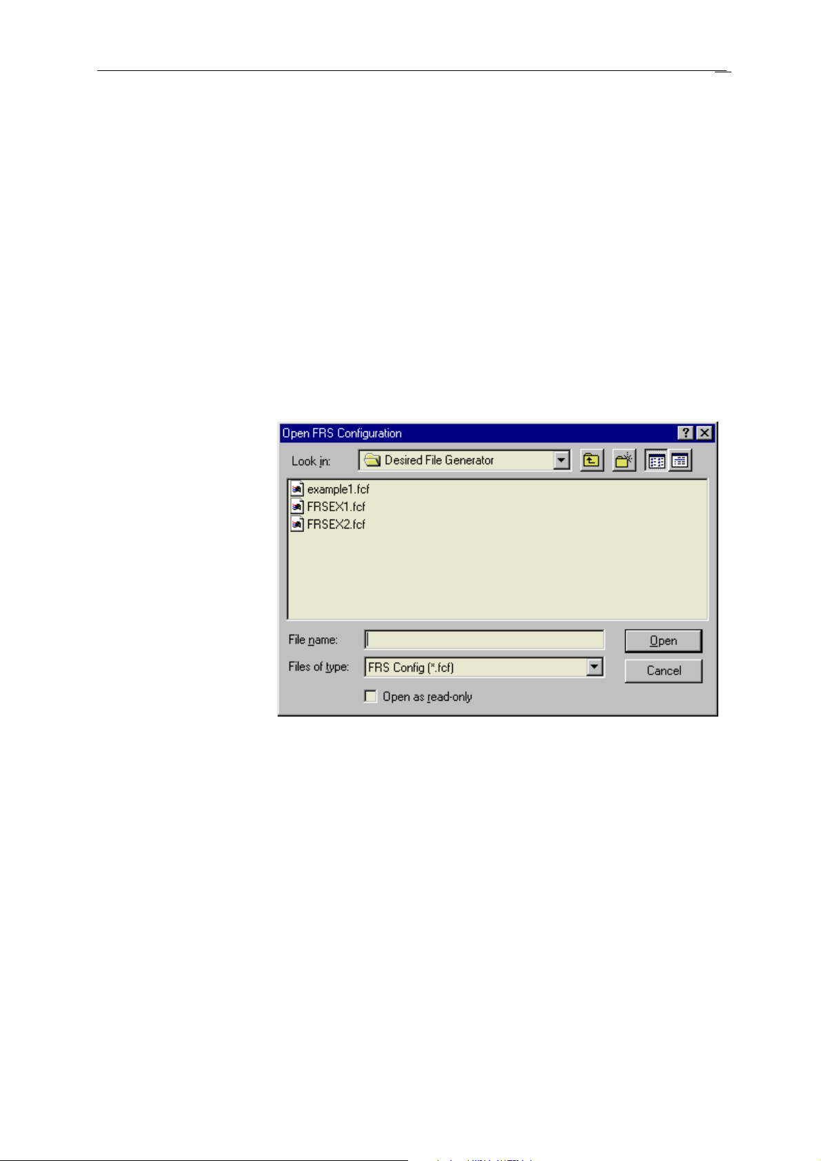
Loading the profile
10
9: Loading an RRS profile
To load in an RRS profile select File | Open and select the
required .fcf file. Once done click on the OK button to load the file.
Importing Data from MS EXCEL
Select File | Import .XLS File… and the following dialogue
will appear. Click the ‘Browse’ button to select a MS Excel file to
import data from and select the Worksheet that contains the data.
Page 17
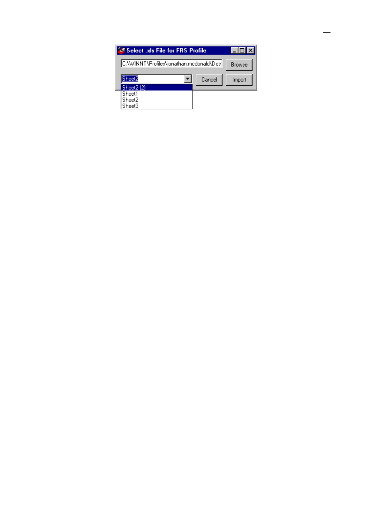
IMPORTANT: The Data in the Excel file MUST be formatted as
described in Appendix A.
The standard import from Excel function requires a full installation
of Excel on the system PC. It is now also possible to import a tab
separated text file by selecting choosing a “text file” option at the file
filter entry when specifying the file name. For multi-channel
applications each channel must be imported separately.
11
Page 18
Using PSD Editor
Servotest’s PSD Editor allows the user to specify one or several target
PSD profiles and generates time histories whose PSD’s are as close as
possible to the targets. In the case of multiple channel PSD, the
corresponding time histories generated are uncorrelated.
Getting Started
After installing DFG a shortcut will have been placed on your desktop
which can be used to run the program. Select the PSD Editor as
shown in Figure 1.
The Main Application Window
The main application window is used to enter the information
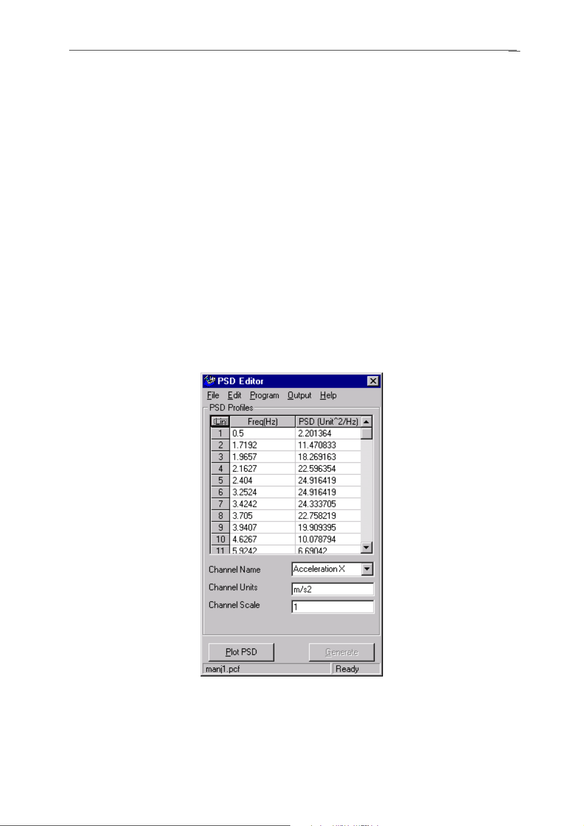
regarding the Power Spectral Density (PSD) profile.
12
Figure 10: FRS Editor main window
PSD Editor loads the last saved PSD profile on starting. If this is the
first time PSD Editor has been used or no profiles have been saved
then fixed default values are loaded into the working PSD profile.
Page 19

• Frequency and PSD Table. Use this table to enter the
frequency in Hertz and the PSD in Units2/Hz.
• Linear and Logarithmic scales. Between two successive
breakpoints, the profile is assumed to be a straight line. However
the user can select either Linear/Linear or Log/Log axes
depending on the toggle button situated at the top left hand corner
of the table.
• Channel Name. Up to 20 characters are allowed. In the case of
multiple channels, use the combo box to switch to another
channel.
• Channel Units. Up to 10 characters are allowed to define the
units of the time history whose PSD is described in the table.
• Channel Scale. If the time history generated is destined to be
used as a drive file using Servotest Replay, the scale entered here
should be compatible with the scale of the drive actuator.
13
Plot PSD
The Plot PSD button is only enabled once data has been entered in the
current PSD profile or after a valid profile file has been loaded.
Selecting the Plot PSD button will open a window containing a plot of
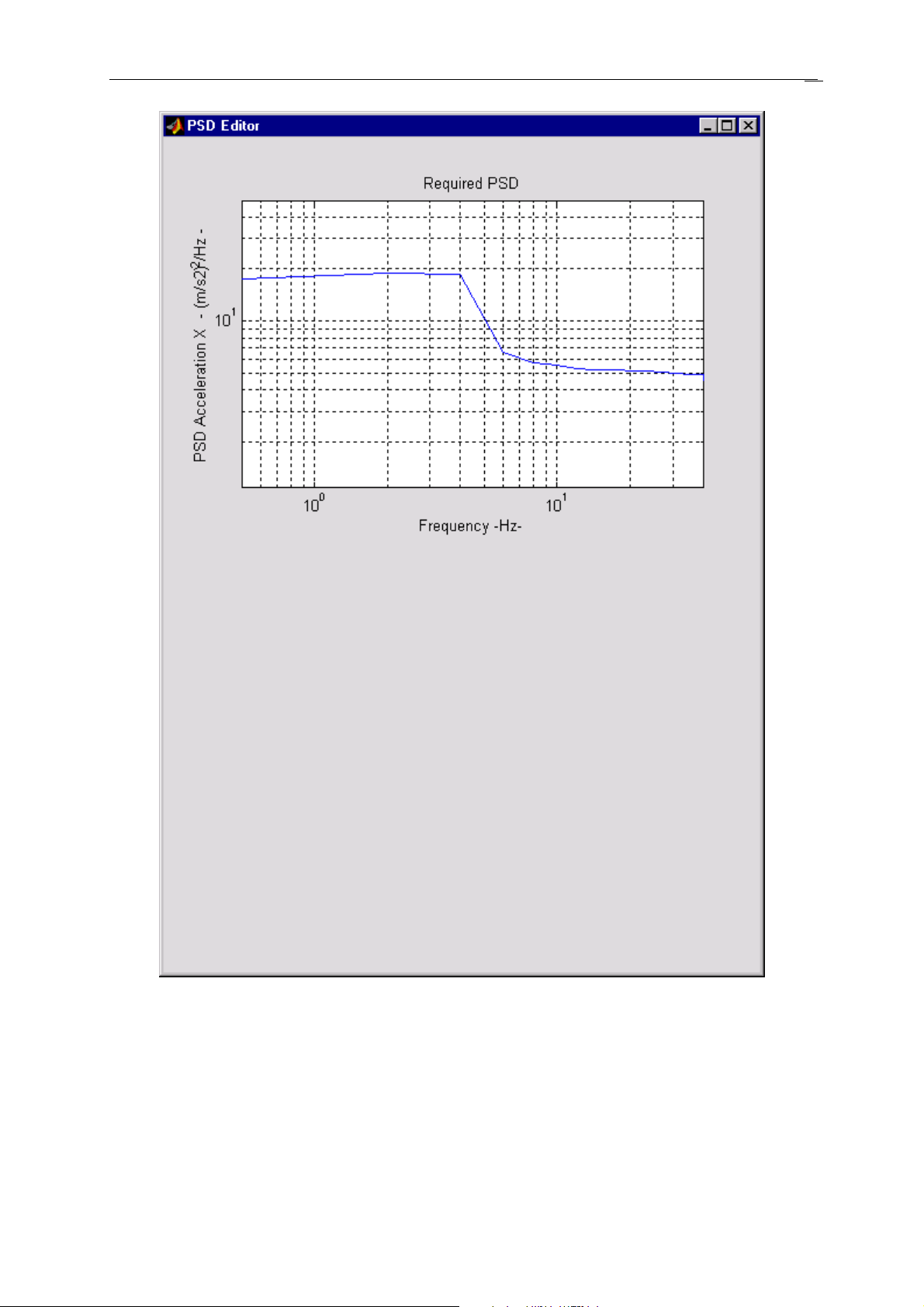
the user entered PSD profile in Linear/Linear or Log/Log reference
axes (see Figure 11).
Page 20
14
Figure 11: Target PSD plot
Generate
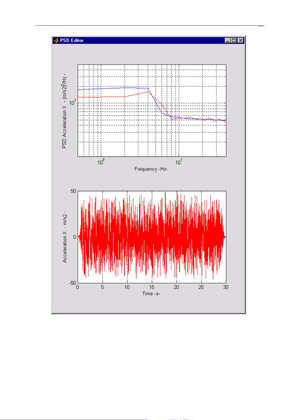
The Generate button is used to generate the time domain waveform(s)
corresponding to the target PSD profile(s) entered. A plot of the time
history corresponding to the current channel is then added to graphics
window and the actual PSD is compared with the target PSD (see
Figure 12 ).
Page 21
15
Figure 12: Target and achieved PSD's and the associated time history
Global Settings
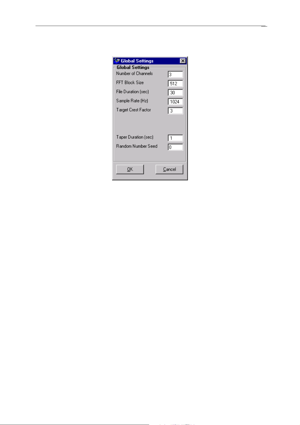
The Output menu contains an element called Global Settings.
Selecting this opens a window (see Figure 13) that allows the user to
set some parameters that are valid for all the channels defined in the
main window. These settings must be selected before the time
histories are generated.
Page 22
16
Figure 13: Global settings
• Number of channels. This specifies the number of PSD
profiles that will be defined and therefore the number of
uncorrelated acceleration waveforms generated.
• FFT Block Size. Values entered in the FFT Block Size edit box
will be rounded to the nearest power of two. A default value of
512 is used if no value is entered. Note that the PSD’s spectral
resolution is given by the ratio: Sample Rate / FFT Block Size.
• File Duration in seconds. It has a default value of 20s.
• Sample Rate in Hertz. This value must be greater than twice
the highest frequency of interest and will default to a value of
102.4Hz.
• Target Crest Factor. In a normalised random set of values (A
white noise file, in this case), the crest factor is a measure of the
deviance of peak values (either maximum or minimum) from the
Standard Deviation of the file. It is calculated as the ratio of the
modulus of the highest or lowest value over the standard
deviation. This value should be no lower than 3.
• Taper Duration in seconds. It has a default value of 3s.
Page 23
Fig
• Random Number Seed. This integer value is used by the
random number generator. A value of ‘0’ generates a unique
sequence of random numbers each time the ‘Generate’ button is
pressed whereas numbers other than zero generate the same
random sequence unique to that Seed Number.
Save Time History
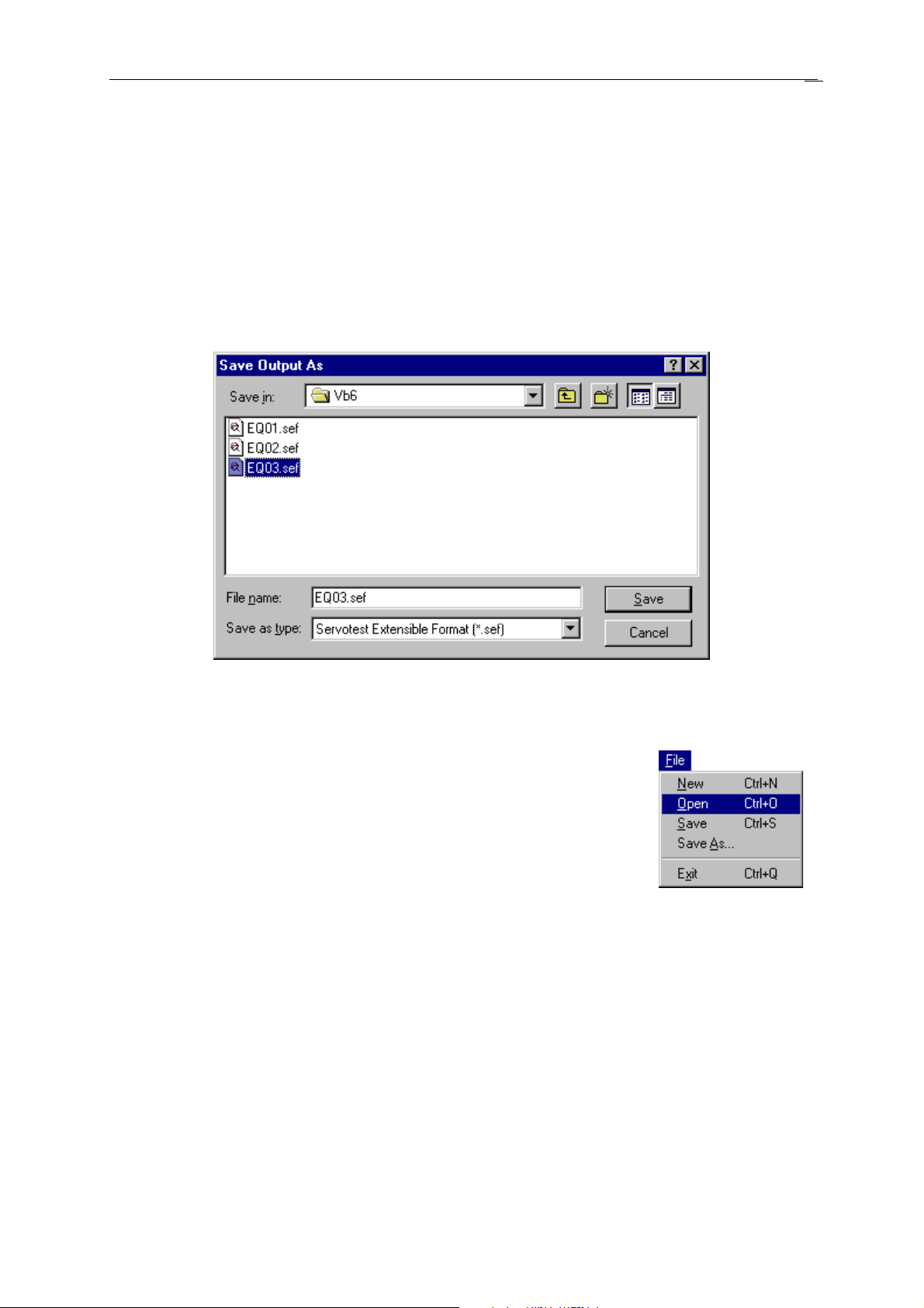
Once the time histories have been generated, they can be saved on
disk by selecting Output | Save Time History and selecting an sbf or
sef file name.
17
PSD Profile Files
PSD profile files are a means by which the
profile data can be stored for retrieval.
On start up PSD Editor will always load the
last PSD profile saved.
New Profile
Selecting File | New clears the frequency and acceleration table
and loads the default values into the other fields ready for a new
profile to be entered.
Saving the profile
Figure 14: Saving the time histories
ure 15: File Menu
Selecting File | Save will prompt the user for a filename if no
profile file is being used, other wise it will save any changes.
Page 24
Figure
Selecting File | Save As will prompt the user for a filename
and save the current RRS profile under that filename.
Loading the profile
18
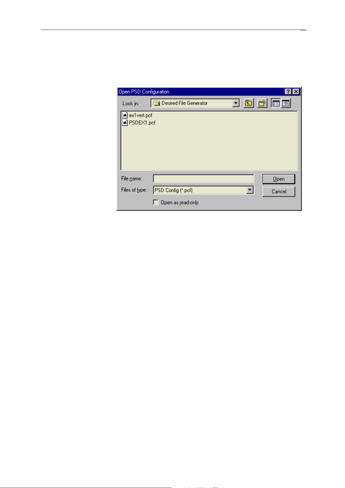
16: Loading a PSD profile
To load in a PSD profile select File | Open and select the
required .pcf file. Once done click on the OK button to load the file.
Page 25
Using Shock Editor
Servotest’s Shock Pulse Editor allows the user to specify the
characteristics of an acceleration shock pulse and, whenever possible,
generates an acceleration time history that meets the specifications.
The acceleration pulse generated is such that both the corresponding
velocity and displacement waveforms have zero initial and final
values.
Getting Started
After installing DFG a shortcut will have been placed on your desktop
which can be used to run the program. Select the Shock Editor as
shown in Figure 1.
19
The Main Application Window
The main application window is used to enter the information
regarding the acceleration pulse.
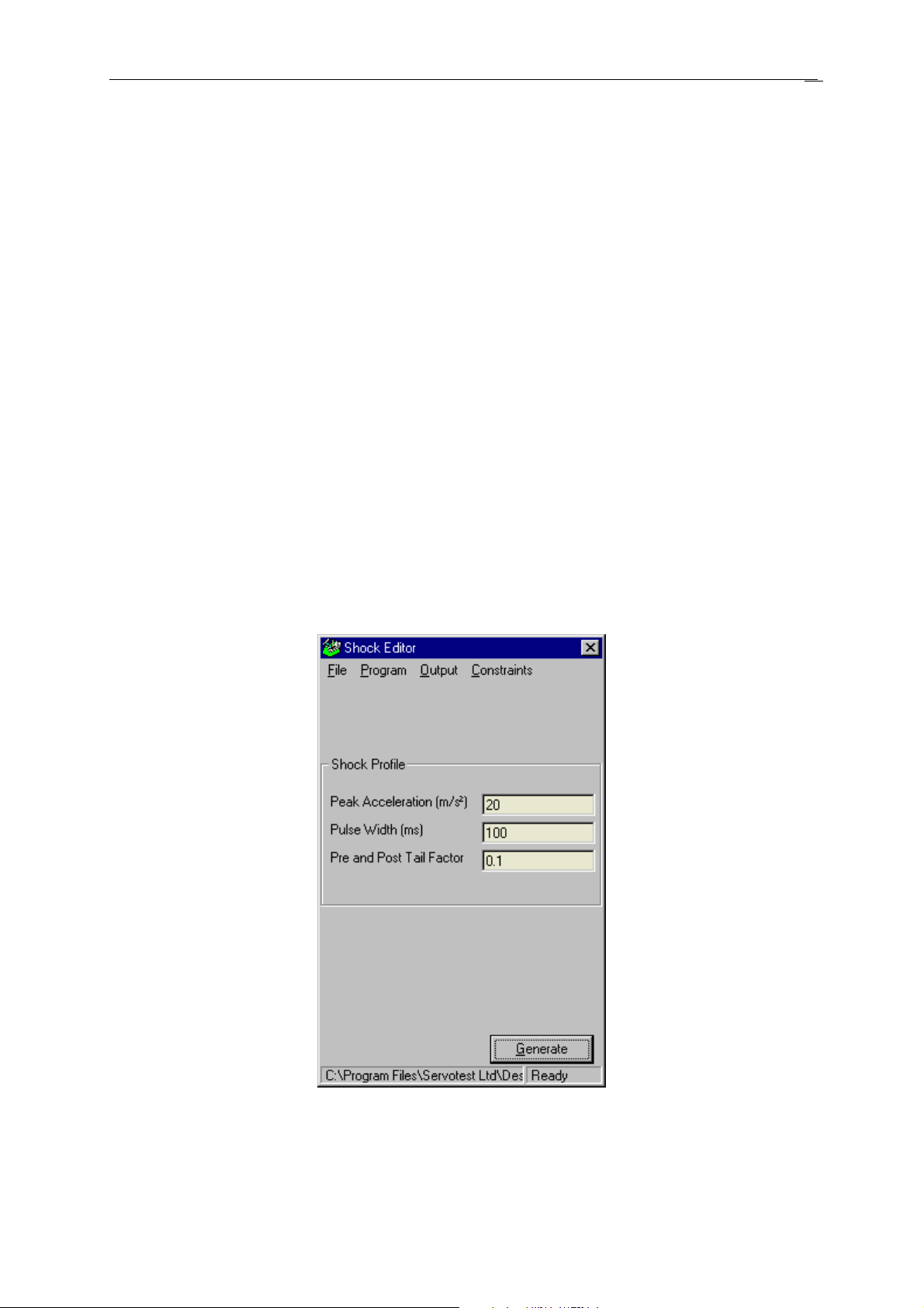
Figure 17: Shock Editor main window
Shock Editor loads the last saved Shock pulse on starting. If this is the
first time Shock Editor has been used or no shock pulses have been
Page 26

saved then fixed default values are loaded into the working Shock
profile.
• Peak Acceleration. The shock pulse is a half sine whose peak
amplitude is entered here in m/s2. This value can be negative.
• Pulse width. This is the duration of the half sine pulse (in ms).
• Pre and Post Tail Factor. In order to achieve zero initial and
final conditions on both velocity and displacement, it is necessary
to use pre and post pulse acceleration shaping waveforms. These
waveforms should not exceed a certain percentage of the peak
acceleration. This percentage is entered here (the value must be
between 0 and 1).
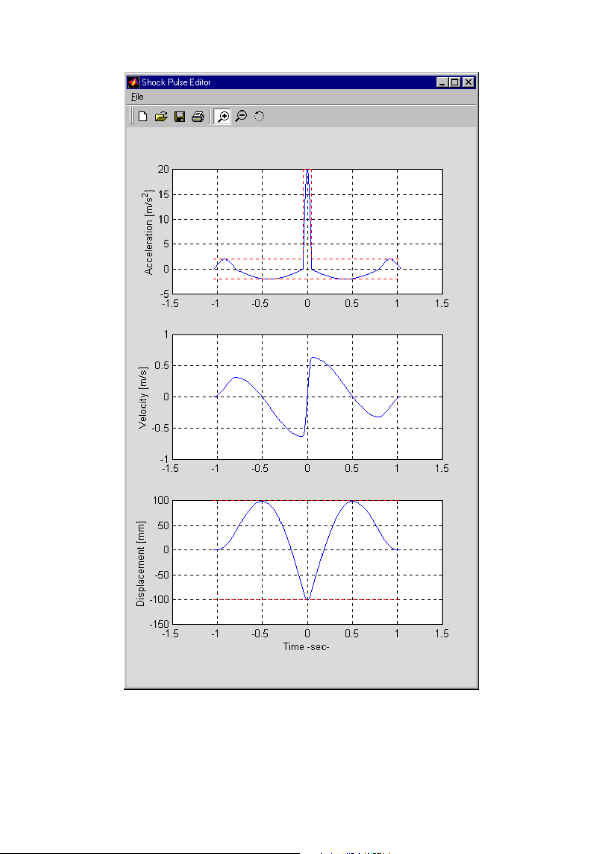
Generate
The Generate button is used to generate the acceleration, velocity and
displacement waveforms corresponding to the target Shock pulse
specified. If a solution is found, these time histories are displayed
together with the constraints (see Figure 18).
20
Page 27
21
Figure 18: Acceleration, Velocity and Displacement waveforms
Page 28
Global Settings
The Output menu contains an element called Global Settings. This is
used to specify the Sample Rate at which the shock pulse is to be
played to the system. Because of the brevity of these pulses it is often
necessary to sample at the highest rate available. By default this is set
to 1024 Hz.
Constraints
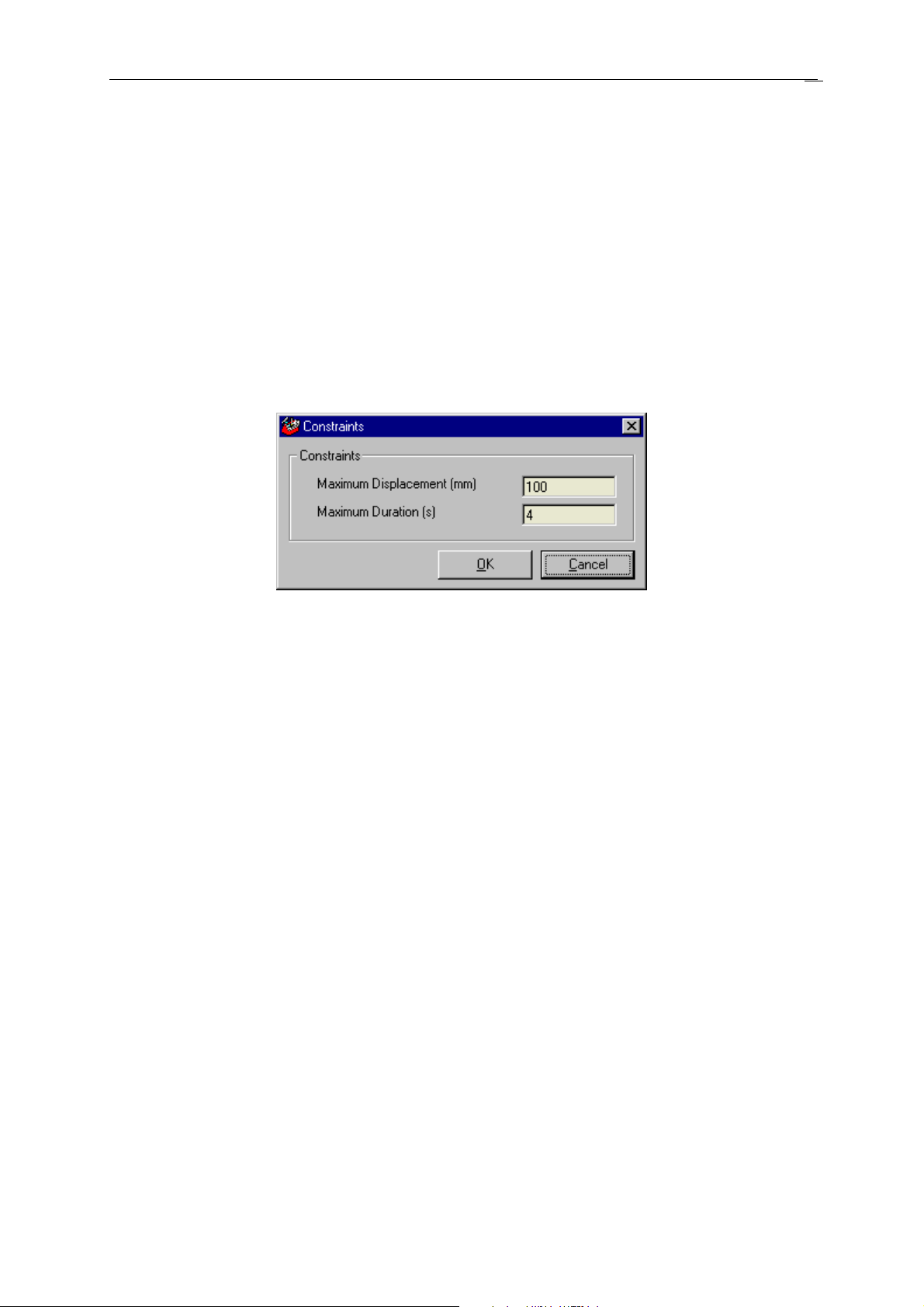
The Constraints menu is used to specify some constraints on the time
histories generated (see Figure 19).
22
Figure 19: The Constraints window
Maximum Displacement. This is the upper limit on the displacement
waveform. This usually corresponds to the actuator stroke (in mm).
Maximum duration. The combination of the pulse and both tails is
not allowed to exceed this value, in seconds.
As the Pulse peak amplitude and duration increase, it becomes more
and more difficult to meet the constraints defined above and the pre
and post tail factor specification. According to how tough the
specifications are, pressing Generate can lead to four possible
situations, as listed below.
1. Unidirectional displacement. All constraints satisfied.
2. Bi-directional displacement. All constraints satisfied.
3. Bi-directional displacement. Maximum duration exceeded.
4. Bi-directional displacement. Tail factor exceeded. Note: a
warning message is then displayed.
5. No solution. An error message is then displayed.
Page 29
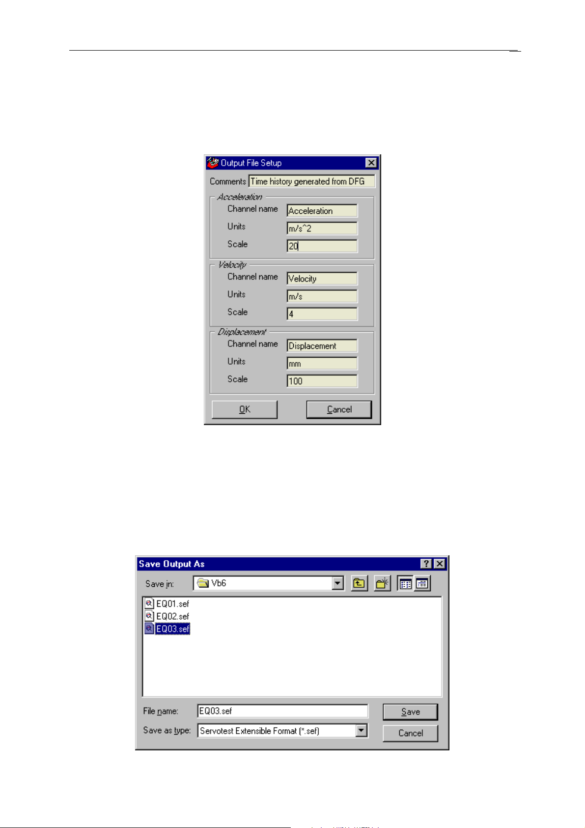
Output File Setup
The Output File Setup window allows the user to specify the Name,
Units and Scale information associated with the Acceleration,
Velocity and Displacement channels to be saved on disk (see Figure
20).
23
Save Time History
Once the time histories have been generated, they can be saved on
disk by selecting Output | Save Time History and selecting an sbf or
sef file name.
Figure 20: Output File Setup window
Page 30
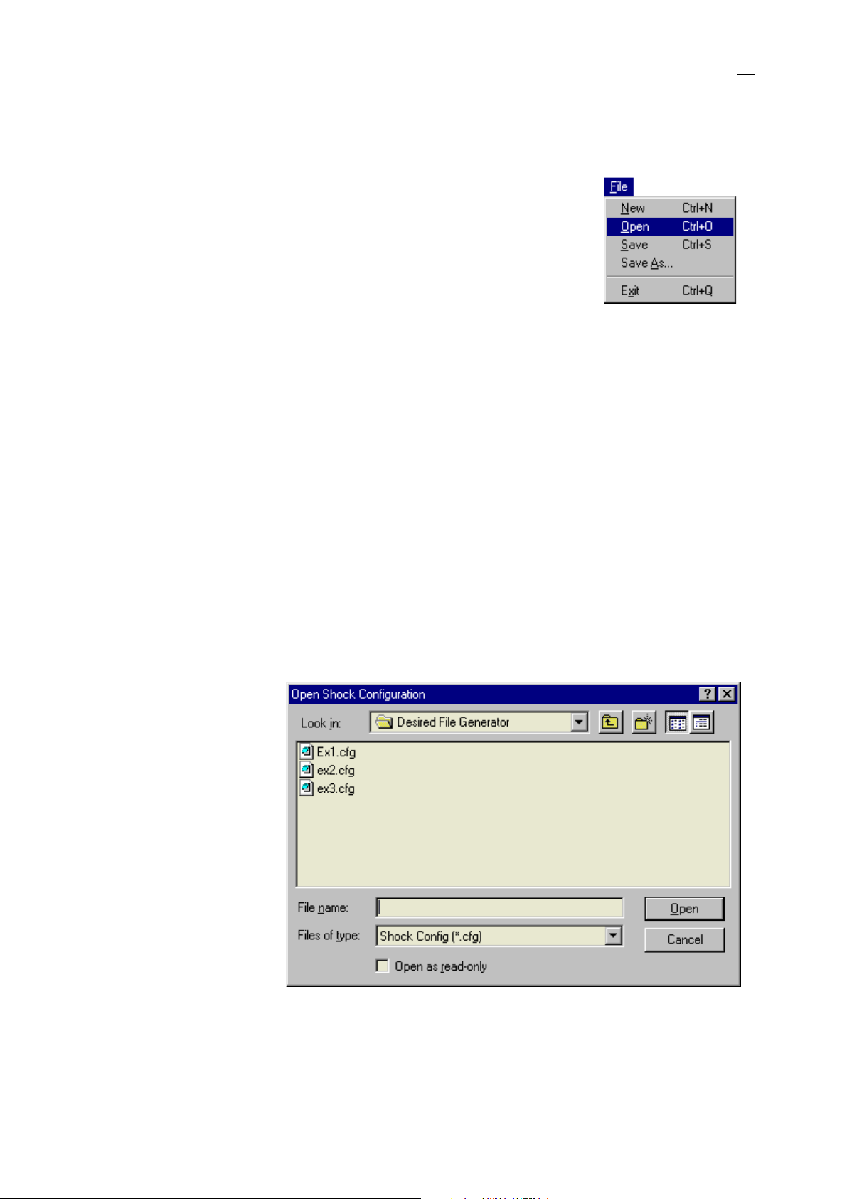
Figure
Figure 21: Saving the time histories
Shock Profile Files
Shock profile files are a means by which the
profile data can be stored for retrieval.
On start up Shock Editor will always load the
last Shock profile saved.
24
New Profile
Selecting File | New clears the frequency and acceleration table
and loads the default values into the other fields ready for a new
profile to be entered.
Saving the profile
Selecting File | Save will prompt the user for a filename if no
profile file is being used, other wise it will save any changes.
Selecting File | Save As will prompt the user for a filename
and save the current Shock profile under that filename.
Loading the profile
22: File Menu
Figure 23: Loading a Shock profile
To load in a Shock profile select File | Open and select the
required .cfg file. Once done click on the OK button to load the file.
Page 31
Using Sweep generator
Servotest’s Sweep generator allows the user to specify one or several
acceleration, velocity or displacement profiles in the frequency
domain and generates sinusoidal sweeps whose amplitudes follow the
profile specified.
Getting Started
After installing DFG a shortcut will have been placed on your desktop
which can be used to run the program. Select the Sweep generator as
shown in Figure 1.
The Main Application Window
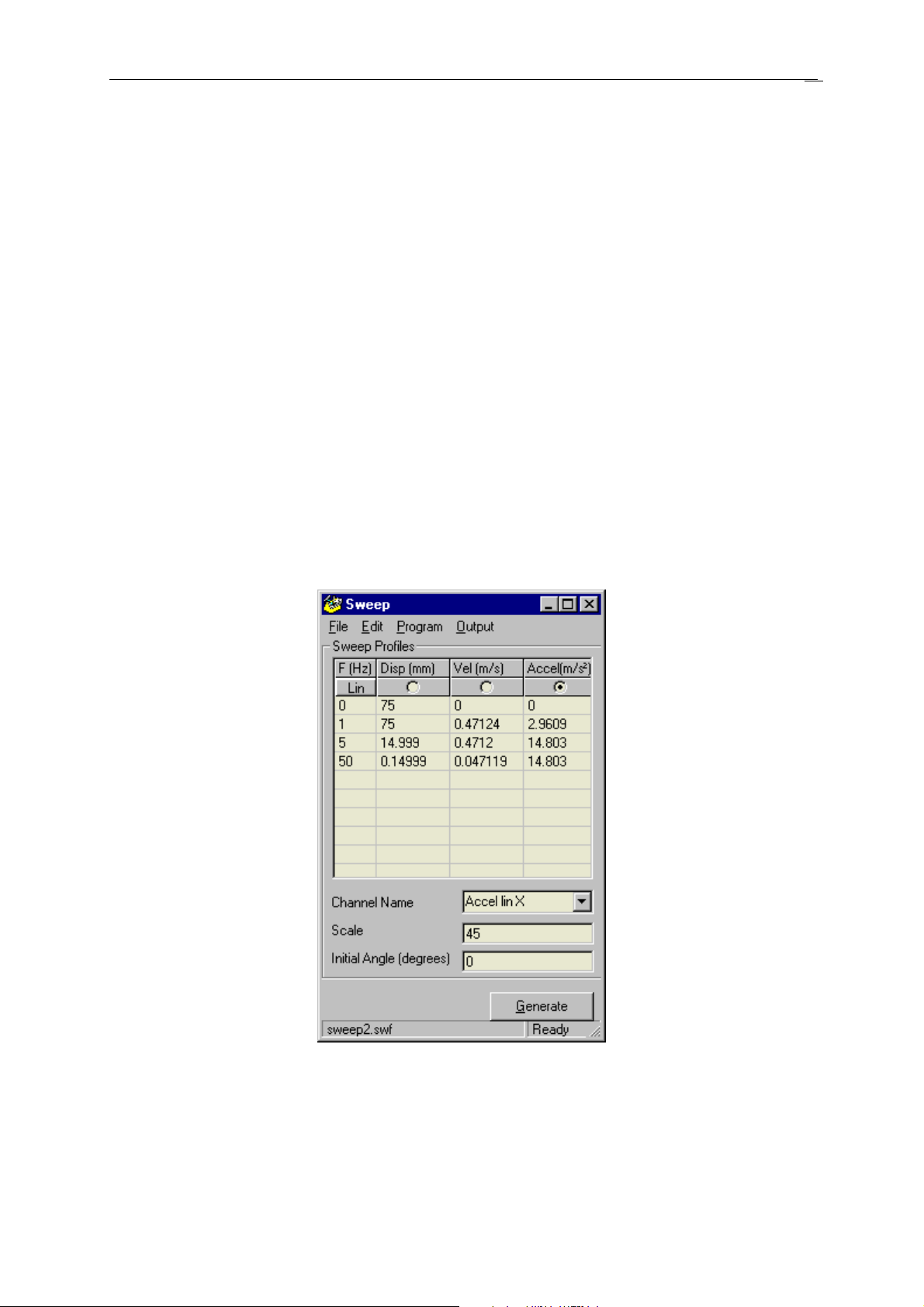
The main application window is used to enter the information
regarding the Sweep profile.
25
Figure 24: Sweep generator main window
Sweep generator loads the last saved Sweep profile on starting. If this
is the first time Sweep generator has been used or no profiles have
been saved then fixed default values are loaded into the working
Sweep profile.
Page 32

• Frequency and Amplitude Table. Use this table to enter the
sweep breakpoint frequencies in Hertz and the corresponding
amplitudes in either displacement, velocity or acceleration. As one
of these three values is entered, the other two are automatically
calculated and displayed (for each breakpoint, the frequency must
be specified before the amplitude).
Note: An empty table generates a zero time history whose
duration is specified in the Global Settings window.
• Linear and Logarithmic sweeps. The user can select either
Linear or Logarithmic sweeps depending on the toggle button
situated at the top left hand corner of the table. The sweep type is
channel dependent.
• Channel Name. The channel name can be changed inside the
list box. Once the user has changed the name of the selected
channel, the user must click OUTSIDE the list box for the
alteration to be registered.
26
Global Settings
The Output menu contains an element called Global Settings.
Selecting this opens a window (see Figure 13) that allows the user to
set some parameters that are valid for all the channels defined in the
main window. These settings must be selected before the time
histories are generated.
• Sweep Mode. For each channel, the user must specify whether
the sweep to be generated should be in displacement, velocity or
acceleration. This is done via the radio buttons found at the top of
the table.
• Channel Scale. If the time history generated is intended to be
used as a drive file using Servotest Replay, the scale entered here
should be compatible with the scale of the drive actuator.
• Initial Angle. The sweep follows the sine funcion so an initial
angle set to zero ensures that the waveform starts at zero when the
sweep is towards high frequencies (Up direction) or finishes at
zero when the sweep is towards low frequencies (Down
direction). The initial angle can be set to any other value in
degrees.
Page 33
27
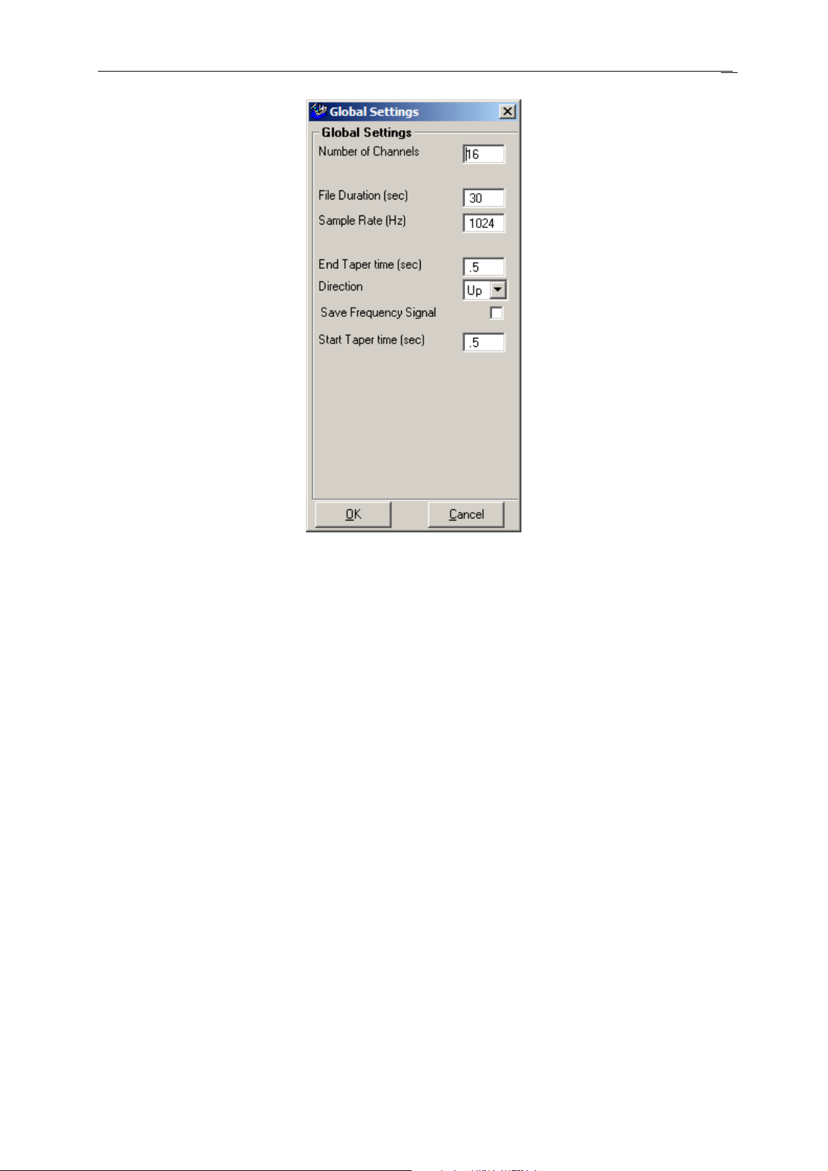
Figure 25: Global settings
• Number of channels. This specifies the number of PSD
profiles that will be defined and therefore the number of
uncorrelated acceleration waveforms generated.
• File Duration in seconds. This is the length of time in which
the sweeps defined for all channels are fitted, including the tapers.
• Sample Rate in Hertz. This value must be greater than twice
the highest frequency of interest and will default to a value of
102.4Hz.
• Start Taper Time in seconds. Use of a start taper is
recommended.
• End Taper Time. in seconds. Use of an end taper is
recommended.
• Direction. Up indicates the sweep starts at low frequencies,
Down indicates it starts at high frequencies.
• Save Frequency Signal. When checked additional
channels are added to the saved file with frequency data for each
main channel.
Page 34
Generate
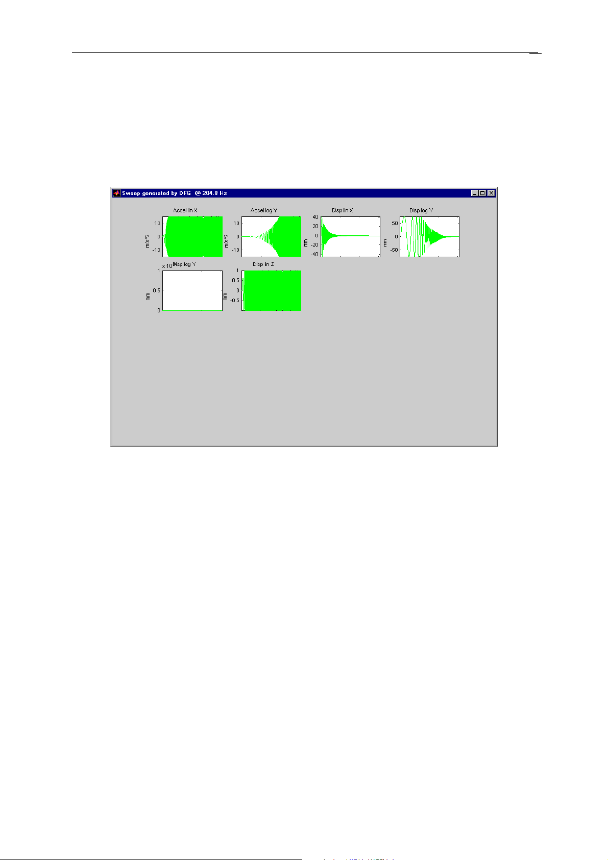
The Generate button is used to generate the time domain waveform(s)
corresponding to the target sweep profile(s) entered. All channels are
displayed on a single graph (see Figure 26). Use DAP to closely
inspect these channels individually.
28
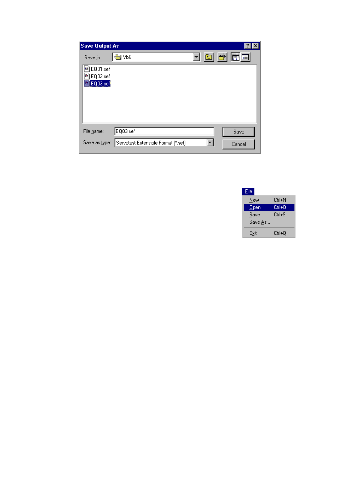
Save Time History
Once the time histories have been generated, they can be saved on
disk by selecting Output | Save Time History and selecting an sbf or
sef file name.
Figure 26: A six channel sweep file
Page 35
Figure
Figure 27: Saving the time histories
29
Sweep Profile Files
Sweep profile files are a means by which the
profile data can be stored for retrieval.
On start up Sweep generator will always load
the last Sweep profile saved.
New Profile
Selecting File | New clears the frequency and acceleration table
and loads the default values into the other fields ready for a new
profile to be entered.
Saving the profile
Selecting File | Save will prompt the user for a filename if no
profile file is being used, other wise it will save any changes.
Selecting File | Save As will prompt the user for a filename
and save the current sweep profile under that filename.
28: File Menu
Loading the profile
Page 36
Figure
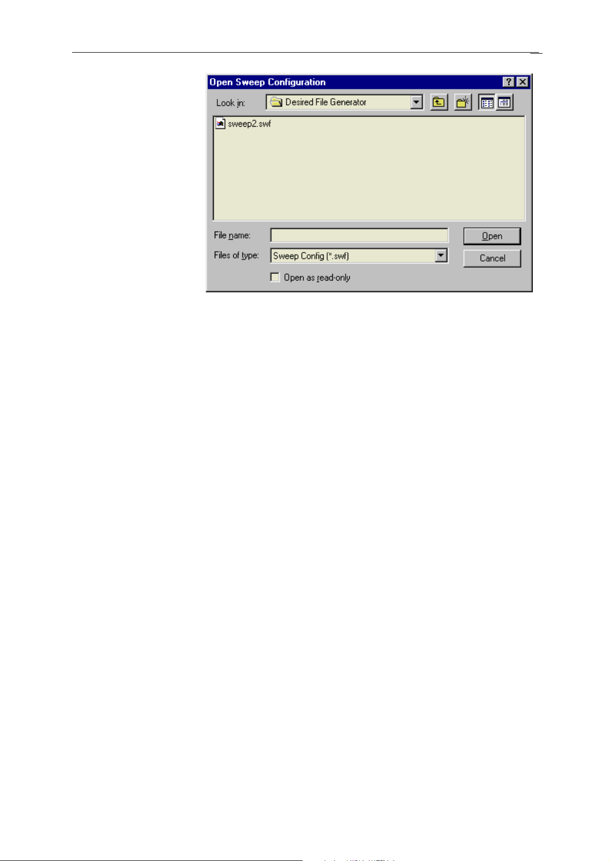
29: Loading a sweep profile
To load in a Sweep profile select File | Open and select the
required .swf file. Once done click on the OK button to load the file.
30
Page 37
Appendix A Edit Menu Options
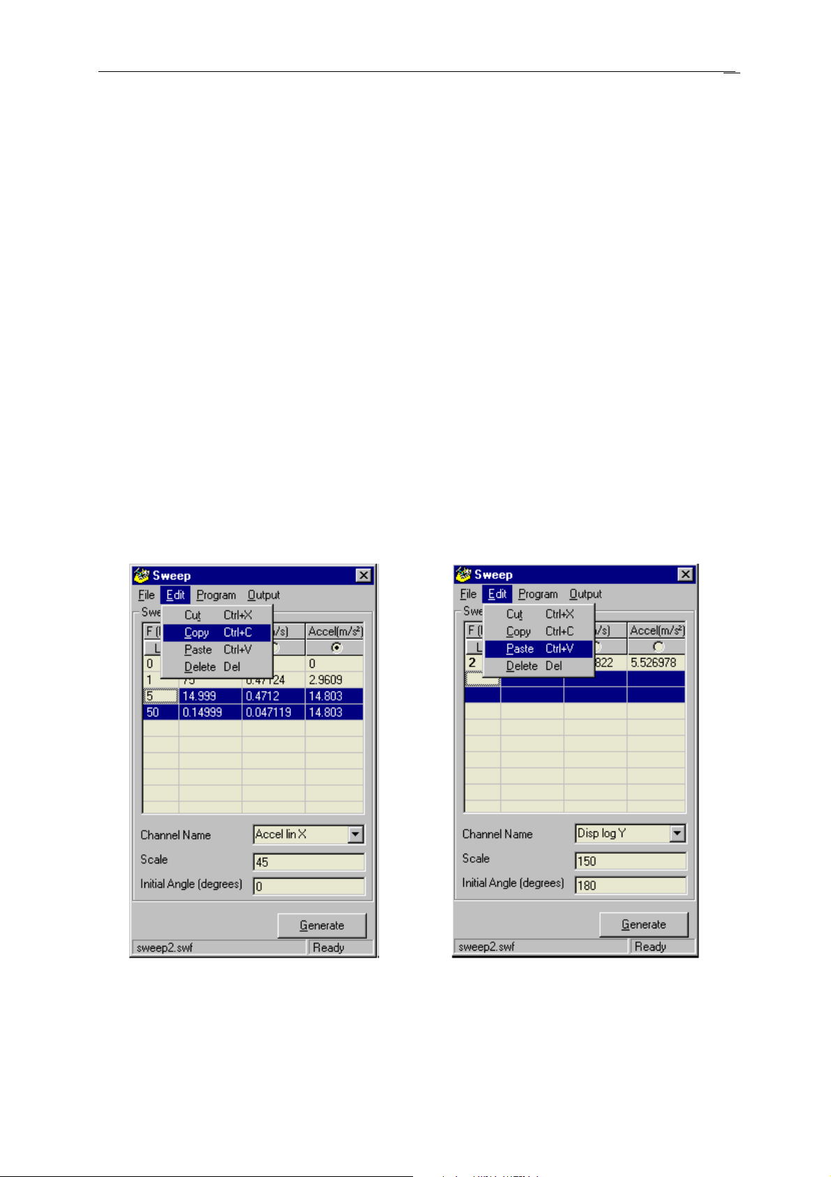
The Edit menu contains Copy, Cut, Paste and Delete commands that
can be used to expedite the process of filling in the tables in the case
of multiple channels.
For example, to copy part of a profile from one channel to another,
proceed as follows:
1. Highlight the cells to be copied and select Copy (see Figure 30 -
left).
2. Select the channel in which to paste the profile
3. Highlight the area in which to paste the profile and select Paste
(see Figure 30 - right).
4. After copying individual cells, click ONCE on the target cell to
select it, then click Paste in the Edit menu. In order for the other
cells at that frequency to be calculated, double click on the cell
you’ve just pasted data into and then click elsewhere.
31
Figure 30: Copying and Pasting using the Edit options
Page 38
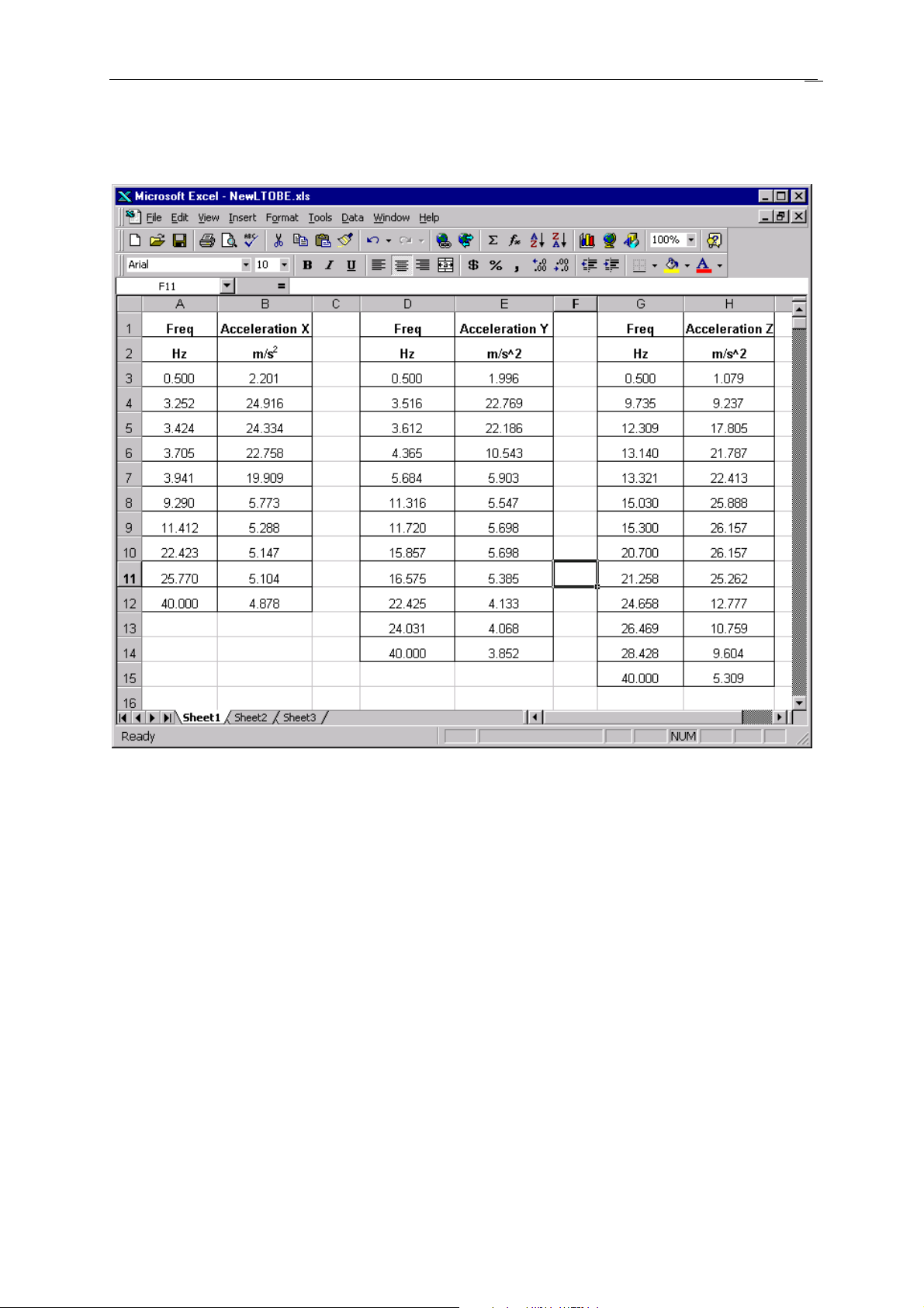
Appendix B Excel Spreadsheet Format for
Importing to DFG
32
Notes:
• Each channel must be separated by 1 blank column.
• The 1st column in each channel must contain the Frequency break points and the 2nd
column must contain the Amplitudes at these frequencies.
• The 1st row of each channel must contain text or numerals. The 2nd cell in the 1st row of
each channel is used as the Channel Name.
• The 2nd row of each channel must contain text or numerals. The 2nd cell in the 2nd row of
each channel is used as the Channel Units.
Page 39

Appendix C Contacting Servotest
Servotest Testing Systems Ltd
Unit 1 Beta Way
Thorpe
TW20 8RE
Telephone: +44 (0) 1784 274410
Fax: +44 (0) 1784 274438
Software support line: +44 (0) 1784 274410
Fax: +44 (0) 1784 274438
E-mail: [email protected]
[email protected]
33
 Loading...