Sensortech Systems ST-3300 Series Technical Manual

Download

ST-3300 Smart RF Sensor

Technical Manual

2221 E. Celsius Avenue, Unit B

Oxnard, California USA 93030

Tel (805) 981-3735

Fax (805) 981-3738

info@Sensortech.com www.Sensortech.com

ST-3300 Smart RF Sensor Technical Manual

Sensortech Systems, Inc. is disclosing this material to you solely for use to operate hardware devices and software we manufacture. You may not reproduce, distribute, republish, download, display, post, or transmit the documentation in any form or by any means including, but not limited to, electronic, mechanical, photocopying, recording, or otherwise, without the prior written consent of Sensortech Systems. Sensortech Systems expressly disclaims any liability arising out of your use of the documentation. Sensortech Systems reserves the right, at its sole discretion, to change the documentation without notice at any time. Sensortech Systems assumes no obligation to correct any errors contained in the documentation, or to advise you of any corrections or updates. Sensortech Systems expressly disclaims any liability in connection with technical support or assistance that may be provided to you in connection with the information.

THE DOCUMENTATION IS DISCLOSED TO YOU “AS-IS” WITH NO WARRANTY OF ANY KIND. SENSORTECH SYSTEMS MAKES NO OTHER WARRANTIES, WHETHER EXPRESS, IMPLIED, OR STATUTORY, REGARDING THE DOCUMENTATION, INCLUDING ANY WARRANTIES OF MERCHANTABILITY, FITNESS FOR A PARTICULAR PURPOSE, OR NONINFRINGEMENT OF THIRD PARTY RIGHTS. IN NO OCCURRENCE WILL SENSORTECH SYSTEMS BE LIABLE FOR ANY CONSEQUENTIAL, INDIRECT, EXEMPLARY, SPECIAL, OR INCIDENTAL DAMAGES, INCLUDING ANY LOSS OF DATA OR LOST PROFITS, ARISING FROM YOUR USE OF THE DOCUMENTATION.

Sensortech, the Sensortech.com logo, and other designated brands included herein are trademarks of Sensortech Systems, Inc. All other trademarks are the property of their respective owners.

Screen 2 of 60

ST-3300 Smart RF Sensor Technical Manual

Preface

About The Manual

This manual is intended to provide a technical reference for configuring and operating the newest Sensortech ST-3300 Series Smart RF Sensors and software. Installation guidelines are provided in the Wiring and Installation document provided with the Sensor. New and experienced users will benefit from the detailed technical information and operating instructions for Sensortech hardware and software options and accessories.

In this manual, the ST-3300 Series Smart RF Sensors are also referred to by the general term “Gauge”.

Hardware Revisions and Software Versions covered by this manual:

ST-3300 Series Hardware Revision: A (and above)

ST-3300 Series Firmware Version: 0.04 (and above)

ST-3300 Series Configuration Software Version: 1.000 (and above)

The manual is organized as follows:

1. Quick Start Guide

2. Sensor and hardware installation information.

3. Sensortech software installation and PC requirements.

4. Overview of the Sensor and software configuration.

5. Overview of Product Calibration using the Sensor.

6. APPENDIX.

7. RS-485 ModBus Specifications

Screen 3 of 60

ST-3300 Smart RF Sensor Technical Manual

Table of Contents

Preface ........................................................................................................................................................................3

About The Manual ..............................................................................................................................................3

Table of Contents .......................................................................................................................................................4

Introduction ................................................................................................................................................................6

Sensor Physical Installation ........................................................................................................................................6

System Overview ........................................................................................................................................................6

Sensor Electronics ......................................................................................................................................................8

Resonant Frequency Dielectric Measurement ................................................................................................ 11

Open Frame Planar Sensor Antenna Measurement ....................................................................................... 16

Sensor Antenna Design ........................................................................................................................................... 19

Theory of Operation ................................................................................................................................................ 20

Radio Frequency Dielectric Measurement ...................................................................................................... 20

Moisture Determination by Dielectric Measurement ..................................................................................... 21

ST-3300 Configuration Software ............................................................................................................................. 22

Minimum Host PC Requirements .................................................................................................................... 22

Software installation ....................................................................................................................................... 22

Connecting to the Sensor using the RS-485 Interface ............................................................................................. 23

RS-485 Serial Communication - Host PC/PLC/Controller to I/O Unit .............................................................. 23

ST-3300 Configuration Program Operation ............................................................................................................. 24

Main Screen – at Startup ................................................................................................................................. 24

Main Screen – Sensor Connected .................................................................................................................... 25

Setup Screen .................................................................................................................................................... 27

Diagnostics Screen ........................................................................................................................................... 28

Measure Configuration Screen ........................................................................................................................ 30

Product Configuration Screen ......................................................................................................................... 34

I/O Configuration Screen ................................................................................................................................. 35

Calibration Screen ........................................................................................................................................... 36

Offset Mode ..................................................................................................................................................... 37

Offset Calibration Procedure ........................................................................................................................... 38

Linear Mode ..................................................................................................................................................... 38

Screen 4 of 60

ST-3300 Smart RF Sensor Technical Manual

Suggestions for taking product samples.......................................................................................................... 40

Maintenance Screen ................................................................................................................................................ 41

Pre-Zero Calibration ................................................................................................................................................ 42

Standardize Calibration ........................................................................................................................................... 43

Pre-Zero Calibration Procedure - using the Configuration Program ....................................................................... 44

Standardize Calibration Procedure - using the Configuration Program .................................................................. 44

Pre-Zero Calibration Procedure - using the I/O Unit Push-buttons ........................................................................ 45

Standardize Calibration Procedure - using the I/O Unit Push-buttons ................................................................... 45

Appendix .................................................................................................................................................................. 46

Sensor Electronics Unit External Connectors .................................................................................................. 46

I/O Unit External Connectors .......................................................................................................................... 47

I/O Unit Terminal Board Layout ...................................................................................................................... 48

I/O Unit Terminal Board Signals ...................................................................................................................... 49

Sensor Status and Error Messages .................................................................................................................. 50

ST-3300 Sensor RS-485 Communications Interface Specification ........................................................................... 51

ST-3300 MODBUS-RTU Serial Communications Interface............................................................................... 51

Screen 5 of 60

ST-3300 Smart RF Sensor Technical Manual

Introduction

Thank you for choosing Sensortech for your moisture measurement and analysis needs. The Sensortech ST-3300 Series of Smart RF Sensors are designed for use in industrial environments and provide the most sophisticated on-line Sensors available, offering unmatched accuracy and reliability.

The Sensors are shipped with all the accessories and custom options ordered. Please compare the contents with the packing list to ensure all items are accounted for. If any items are missing or damaged, please contact Sensortech immediately for further assistance.

Sensor Physical Installation

Every Sensor installation is unique and specific installation instructions are provided for the most common and custom Sensor Application Interfaces. Please refer to the ST-3300 Wiring and Installation Guide for your specific application.

System Overview

The ST-3300 Series Sensor is a complete measurement and interface system where all signal processing and control functions are self-contained. It features multiple interface protocols including one isolated 4-20mA output, an RS-485 serial communication port, a Digital Input and a Product Temperature Input. Optional communications protocols include OI-6000 Operator Interface, Ethernet TCP/IP, DeviceNet, PROFIBUS, PROFINET and EtherNet/IP as well as digital inputs and outputs for external sample gating and control.

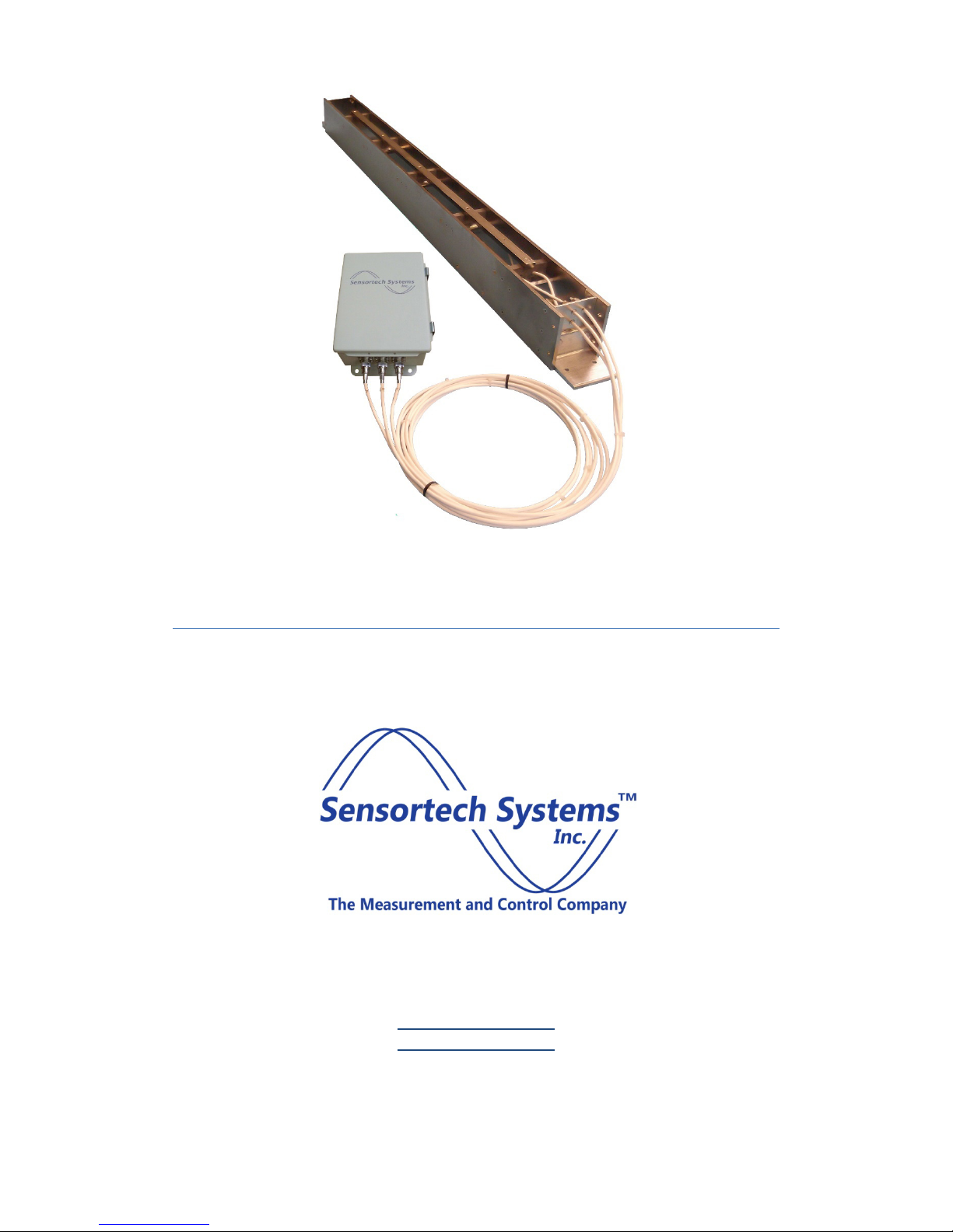
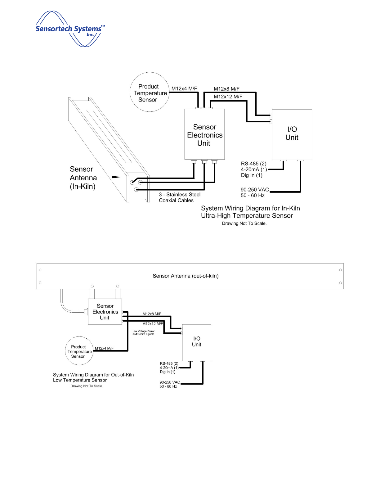
The ST-3300 System is composed of the following components:

Sensor Antenna - an antenna that is located in close proximity to the Product being measured and is either directly attached for low temperature applications or remotely located for high temperature applications. The Sensor Antenna is connected to the Sensor Electronics Unit through coaxial cables.

Sensor Electronics Unit - a NEMA rated metal enclosure which houses 2 PCB’s – the RF PCB and the Processor PCB. The RF PCB generates signals sent to the Sensor Antenna and provides frequency and voltage signals to the Processor PCB for moisture and temperature value calculations. It connects to the I/O Unit and the Sensor Antenna via M12 for power and signals as well as coaxial cables to measure product moisture. The Processor PCB controls the RF PCB and to read and manage data on the analog and digital interfaces.

I/O Unit - a NEMA rated metal enclosure which provides +/-15VDC power to the Sensor and allows the user to install wires onto the terminal blocks and connectors mounted on the I/O Unit PCB to provide AC power and external analog and digital interfaces.

Product Temperature Transducer - a user defined peripheral pyrometer or transducer module that connects to the Sensor Electronics Unit via a M4 x 4 pin connector for 4-20mA or voltage input via an M12 x 4 cable.

Screen 6 of 60

ST-3300 Smart RF Sensor Technical Manual

Figure 1: Example of In-Kiln Open Frame Planar Sensor System

Figure 2: Example of Out-of-Kiln Open Frame Planar Sensor System

Screen 7 of 60

ST-3300 Smart RF Sensor Technical Manual

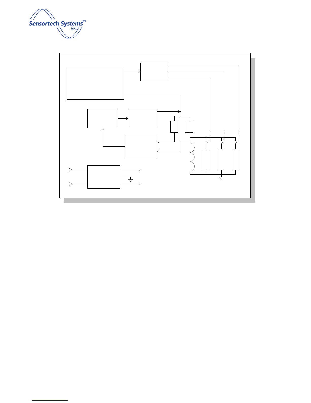
Sensor Electronics

The heart of the ST-3300 is a sophisticated dielectric Sensor. The Sensor utilizes state of the art phase lock loop technology. High speed logic and ultra-high bandwidth operational amplifiers enhance performance. A microprocessor controls the RF measurement circuit and communicates with user defined protocol interfaces. Figure 3 shows a block diagram of the Sensor electronics.

Measurement is made by switching between one of three RF channels: CA, CH, CL and Sensortech Systems

developed and patented a specific method of dielectric determination using radio frequency. This is known as the resonant frequency technique. The purpose of the reference channels is to stabilize the Sensor over a wide range of ambient conditions. The three frequencies are measured by an onboard microprocessor and form the inputs to a proprietary algorithm used to eliminate most drift factors.

CA connects to the Sensor Antenna element which is in close proximity to the product being measured. CH

connects to the High Reference element and CL connects to the Low Reference element for precision reference

calculations.

Only one channel is switched in circuit per measurement sample, this forms a parallel tuned circuit with the inductor. The resonant frequency of this network constitutes the "lock frequency" of the phase lock loop.

Screen 8 of 60

ST-3300 Smart RF Sensor Technical Manual

Opto/

A/R Sw

Isolator

Micro-processor and

Control Logic

Driver/

Freq. out

+12v

-12v

Isolator

Voltage

Controlled

Oscillator

Isolated Power Supply

Pin Diode Drivers

Automatic Gain Control

R R

Phase

Detector

+5v

-5v

Figure 3: Sensor RF PCB Block Diagram

The block diagram of Figure 3 shows the inductor L forming a parallel tuned circuit with one of three channel capacitances, C

. One capacitor is the Sensor electrode next to the product and the other two are reference

frequencies. Switching is performed by PIN diodes. The micro-processor sends control signals to measure each channel sequentially.

The resulting frequency measurements are:

FS = Sensor Antenna Frequency

= High Reference Frequency

= Low Reference Frequency

The raw moisture value for Moisture is calculated from the equation:

Moisture = STD * B coefficient * (DR – Pre-Zero) + C coefficient

where: B coefficient = slope

calibration coefficient for Product selected (SPAN)

C coefficient = offset calibration coefficient for Product selected (ZERO)

STD = Standardization Factor (calculated)

= calculated raw dielectric value

Pre-Zero = calculated raw dielectric value with empty Sensor – air only from Pre-Zero Calibration

Screen 9 of 60

ST-3300 Smart RF Sensor Technical Manual

The Sensor measurement results are sent from the Sensor Electronics Unit to the I/O Unit via RS-485 interface. The I/O Unit provides +/-15V power supply for the Sensor Electronics Unit and terminal board connectors for connection of the analog and digital interface signals to the user’s process control systems.

The I/O Unit also provides local push button controls for performing the Zero and Standardize calibrations of the Sensor. The user opens the lid of the enclosure and presses the Zero button with nothing over the Sensor and the Status LED next to the button lights up to indicate a Zero calibration has been performed. The user then places a Standardization Plate over the Sensor and presses the Standardize button. The Status LED next to the button lights up to indicate a Standardize calibration has been performed.

Screen 10 of 60

ST-3300 Smart RF Sensor Technical Manual

Resonant Frequency Dielectric Measurement

Numerous methods have been used to determine dielectric constant of a material. Radio frequency is often used for its ability to penetrate a material to a substantial depth and to be able to measure without contacting the material. Sensortech Systems developed and patented a specific method of dielectric determination using radio frequency. This is known as the resonant frequency technique.

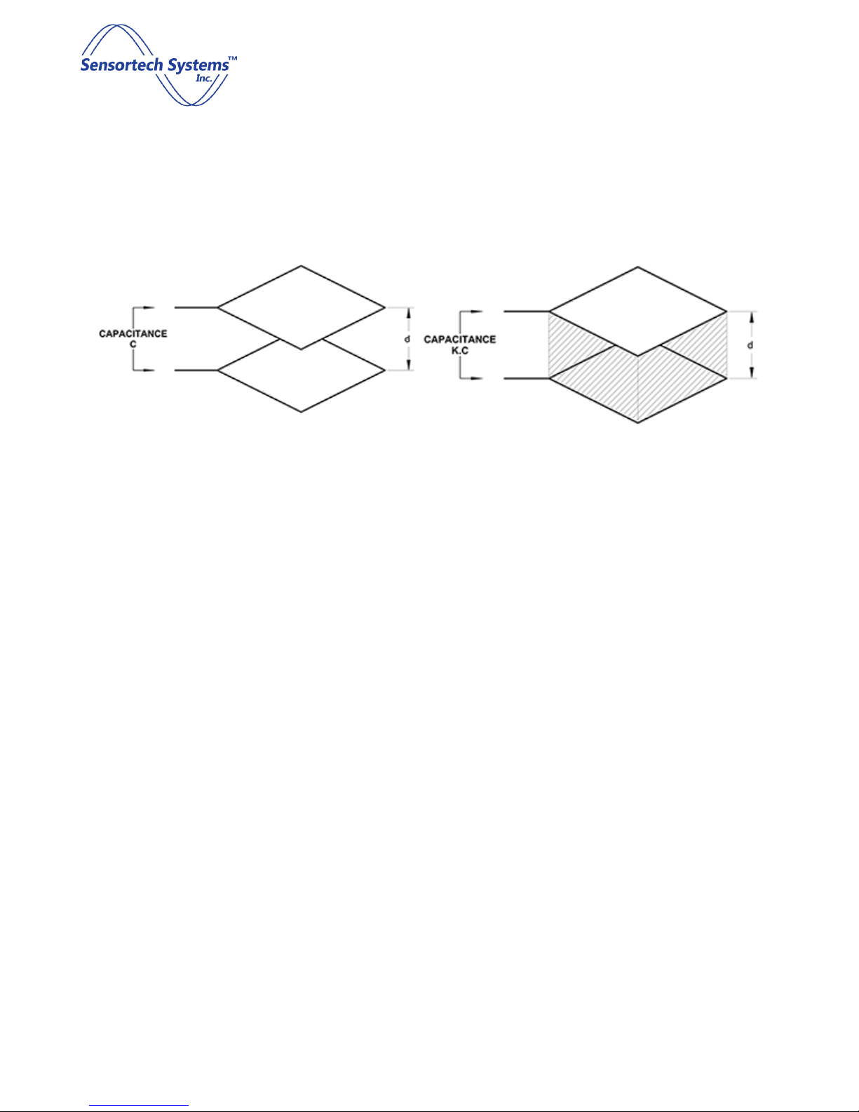
Figure 5: Parallel Plate Capacitor with Dielectric Medium

Figure 4: Parallel Plate Capacitor with Air Medium

As previously stated, dielectric is a material property affecting the way it behaves in an electric field. A parallel plate capacitor is shown in figure 2(a). If the medium separating the plates is air or a vacuum, the capacitance is given by:

C = (ε

A) / d

⋅

where: ε

= permitivitty of free space = 8.854 x 10

-12

A = Area of plate d = separation distance of plates

When a dielectric medium separates the plates as in figure 2(b), capacitance becomes:

C = (ε

⋅

A) / d

⋅

where: ε

= dielectric constant

Thus, capacitance is directly proportional to the dielectric constant of the material in the electric field.

C = K

⋅

Parallel plate capacitance Sensors are rarely used for industrial applications; single-sided Sensors being preferred.

Screen 11 of 60

ST-3300 Smart RF Sensor Technical Manual

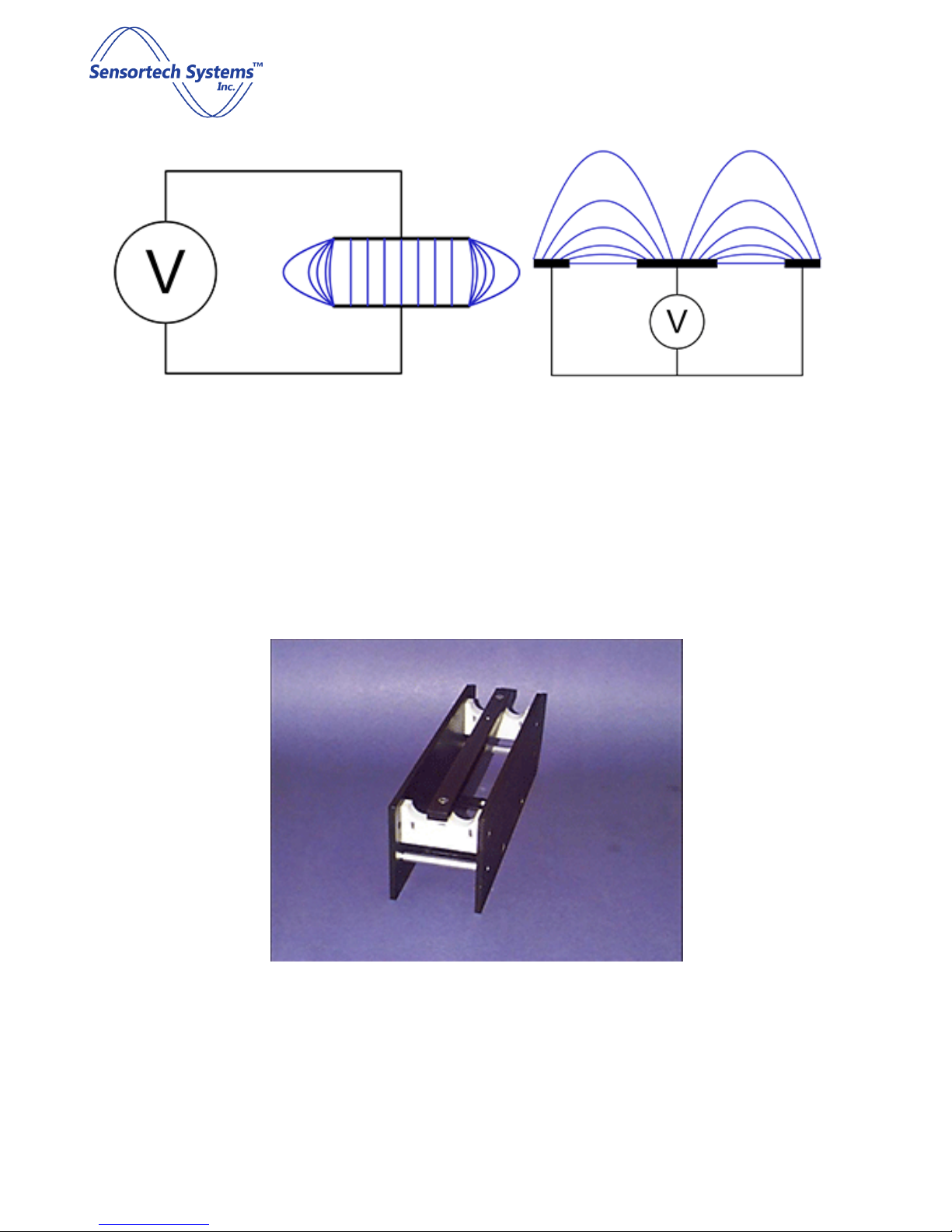
Figure 6: Parallel Plate Capacitor Showing Flux Lines

Figure 7: Planar Sensor Antenna Showing Flux Lines

Figure 6 is schematic representation of a parallel plate capacitor showing uniform electric flux lines except at the edges where fringing occurs. The fringe field is generally undesirable in a capacitor, but in a single-sided capacitance Sensor, it is the only useful field.

Figure 7 is a cross-sectional view of a planar Sensor, most frequently used for gypsum board applications. A central element propagates an electric field to the grounded side plates. A small proportion of the field is directly between electrodes, but most is the fringe field used to penetrate the board. Figure 8 shows an example of an Open Frame Planar Sensor Antenna.

Figure 8: Example of an Open Frame Planar Sensor Antenna

Electrically, the Sensor Antenna, is simply a capacitor. The electrical analogy of the gypsum product is itself a capacitance with parallel resistance. The resistance or conductance represents the ionic conductance or dielectric loss in the board.

Screen 12 of 60

ST-3300 Smart RF Sensor Technical Manual

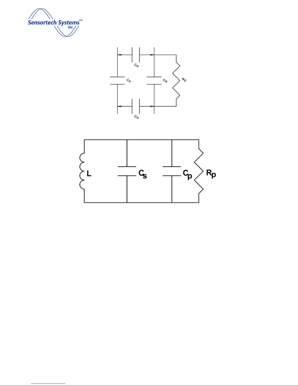
Figure 9: Electrical Schematic of Product Coupling

Figure 10: Electrical Schematic of Equivalent Resonant Circuit

Figure 9 shows the electrical schematic of the product coupled to the capacitive Sensor. Air gap capacitance (

couples the product (

) to the Sensor (

) and must, therefore, be kept constant. Mounting the Sensor

between conveyor rollers, spaced perhaps 6mm below the plane of the rollers, ensures a constant coupling

capacitance, provided rollers are reasonably true. The capacitances may be combined as one (

mathematically incorrect, may simplistically be represented as

CT = Cs + C

) which, while

Figure 10 illustrates the resonant network formed by Sensor capacitance in parallel with product capacitance also in parallel with inductor (L). This network has a unique resonant frequency at which inductive reactance cancels capacitive reactance and network impedance is at a maximum. Impedance at resonance is actually

resistance (

)

Screen 13 of 60

ST-3300 Smart RF Sensor Technical Manual

Figure 11: Electrical Schematic Example of a Resonant Circuit

Figure 12: Frequency, Phase and Impedance relationships of Resonant Network

Screen 14 of 60

ST-3300 Smart RF Sensor Technical Manual

The resonant network is driven from a suitable RF signal through a pure fixed resistor (Ro) as shown in Figure 11. As frequency increases, the network is first of all inductive with a leading phase angle. At resonance all reactive components cancel and the circuit is purely resistive. At resonance, the signal amplitude across the resonant network is a function of only R

, Rp and amplitude of the driving signal. Ro and Rp behave as a simple potential

divider.

Using a precision phase lock loop to adjust signal frequency to maintain zero phase angle across resistor R

ensures the network is always at resonance.

Resonant frequency is defined as:

= 1 / [2π√(L

)]

⋅

The Sensor measures this frequency and a proprietary measurement algorithm combines Sensor frequency with two reference frequencies to produce a dielectric value that is essentially independent of ambient temperatures and component aging.

The resulting raw dielectric can be seen to be a function of Sensor capacitance (with product) and precision reference capacitors. Inductance and stray capacitance are eliminated.

Moisture is directly proportional to the raw dielectric.

Given a linear relationship, the instrument can now be calibrated from analytical data to fit a linear function of the form:

Moisture = a

D + b

⋅

Since capacitance C of Sensor capacitance. This is achieved by measuring Sensor capacitance when no product is present (D

is a composite of both the Sensor and the product, it is necessary to remove the influence

) and

subtracting this from future measurement in a similar way to performing a tare on a weigh scale. This action is termed 'Pre-zero' and should be performed periodically to compensate for antenna changes and product buildup on the antenna.

The primary moisture measurement of the Sensor uses the principle of dielectric determination. Since moisture has a much higher relative dielectric than most solids, it is possible to relate to moisture content. Radio frequency moisture determination, which is a penetrating measurement, has to take into account the mass of the product being measured in order to provide a percentage measurement. This is because the Sensor effectively counts the water molecules within the Sensor field. If more product is squeezed into that field, it will produce a higher moisture reading, even though the percentage water figure may be constant. In order to correct for this, the product mass, weight or density must be taken into consideration.

Screen 15 of 60

ST-3300 Smart RF Sensor Technical Manual

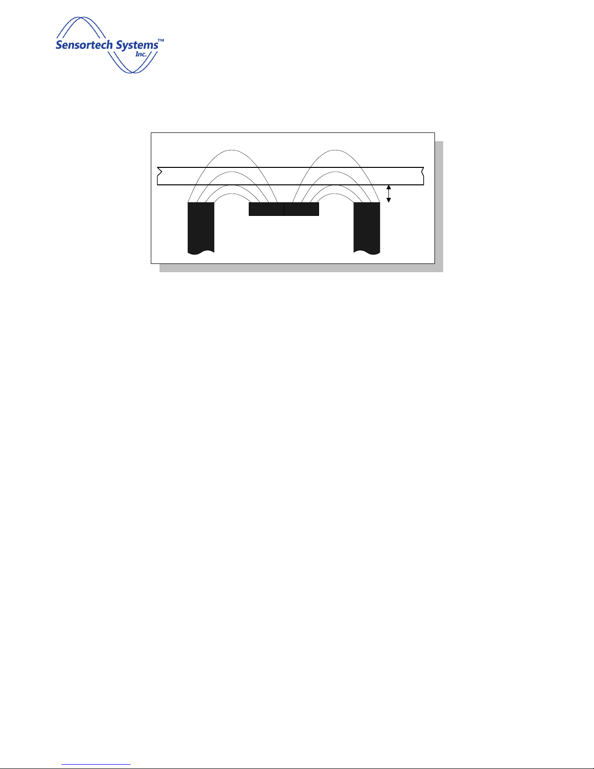
Open Frame Planar Sensor Antenna Measurement

fringe field

product

dielectric

Doc ume

Doc

ume

air

dielectric

Figure 13: Open Frame Sensor - Radio Frequency Field Penetrating Through Product

The Figure 13 shows the typical radio electric field passing through a product. The dielectric effect of the product will be a function of its dielectric constant and the length of flux paths passing through the product (fringe field lines). The latter will be a function of product thickness and distance from the Sensor. If a parallel plate Sensor were used, the field lines would be uniform and a doubling in product thickness would produce a doubling in dielectric. The Sensor shown is a single sided or Planar Sensor Antenna, with a non-linear field. Doubling of product thickness will cause an increase in dielectric, but not by a factor of two. A Planar Sensor Antenna response would be of the form:

Sensor Measurement = Product Dielectric * (Mass)Kw

where: Mass = weight, density, thickness etc. Kw = coefficient determined by antenna geometry (less than 1)

The value of Kw coefficient will depend upon antenna geometry, product presentation and form of mass measurement e.g. thickness, weight etc. To determine Kw, a constant moisture product of varying mass is presented to Sensor. A graph of log (Sensor response) vs. log (mass) must be plotted. Kw is given by the slope of this line (see Figure 14).

Screen 16 of 60

ST-3300 Smart RF Sensor Technical Manual

The product dielectric is coupled to the antenna via an interface such as air. In some cases, direct contact may be made, or a fixed interface such as a Teflon or Ceramic window may isolate the Sensor from the product. The important thing is that the interface between product and Sensor, must remain constant in order for the interface dielectric to be cancelled out of the product measurement. In the case of direct contact or a window, this would be the case. If an air gap exists between product and Sensor and the air gap distance varies, due to mechanical vibration or board bounce, the total dielectric for the measurement will change. If the gap can be measured, it can be compensated.

If the antenna were a point source, then the RF energy would decrease according to the inverse square law and a simple compensation based upon the square of the distance would be possible. In practice the antenna is a finite width radiator producing a more complex relationship. It is further complicated by field distortion through the product.

Instrument

Mass

Figure 14: Plots of Sensor Measurement vs. Product Mass

Kw = log(y)/log(x)

log (Instrument)

log (Mass)

Figure 13 shows the typical field pattern emanating from a planar electrode, but this is somewhat idealized, as the field is actually distorted or refracted within the product. The amount of distortion is a function of product dielectric and is both density and moisture dependent. This distortion will also affect the field in the air gap and the distance relationship.

In practice, the product density usually remains fairly constant at a fixed point in the process, and the moisture similarly should not vary too greatly. If this is the case, distance may be corrected by an equation of the form:

Compensated Sensor = product dielectric * (distance + Kd)2

If moisture and density are uncontrolled such as raw material measurement, it is better to control or constrain the distance variation rather than try to compensate for it.

Screen 17 of 60

ST-3300 Smart RF Sensor Technical Manual

The example to the left shows three Sensor measurements of differing moisture, at varying distances from the Sensor. No compensation is applied and an inverse relationship is apparent.

0 .25 .50 .75

Distance

. In this next example the same three Sensor measurements are

performed at varying distances. The Sensor has a compensation

equation:

Mc = Mu (D + 0.14)2

The offset coefficient Kd (.14) is determined by trial and error to obtain

0 .25 .50 .75

Distance

flattest response.

Figure 15: Plot of Sensor Measurement vs. Product Distance

Screen 18 of 60

ST-3300 Smart RF Sensor Technical Manual

Figure

: Planar Open Frame Sensor Antenna

Sensor Antenna Design

From an electronic standpoint, antenna is a misnomer. A truer description would be electrode or probe, since antennae tend to denote devices designed for maximum propagation efficiency, usually achieved by standing wave theory.

For dielectric measurement, standing waves are to be avoided at all cost since this would produce nonuniform energy distribution. The Sensortech Systems probe is essentially a deliberately mismatched antenna to provide broadband uniform dielectric coupling to product.

Antenna geometry (shape, size, etc.) is mainly a function of application, since provided the above criteria are met, it is largely a matter of mechanical design as how best to couple to the product. Sensortech Systems, Inc. has over a period of years, developed many unique electrode designs including: parallel plate, planar, cylindrical (pipeline), probe and co-axial types. The most widely used style is the planar type shown in figure 2. Consisting of a central electrode between two ground planes, or multiple electrodes interspersed with ground plane, this style provides a single sided measurement preferred in most industrial applications.

Screen 19 of 60

Theory of Operation

Radio Frequency Dielectric Measurement

ST-3300 Smart RF Sensor Technical Manual

Figure 17:Electric field interaction with an atom under the classical dielectric model

In the classical approach to the dielectric model a material is made up of atoms. The atoms consist of a positive point charge at the center surrounded by a cloud of negative charge. The cloud of negative charge is bound to the positive point charge. The atoms are separated by enough distance such that they do not interact with one another. This is represented by the top left of the figure aside. Note: Remember the model is not attempting to

say anything about the structure of matter. It is only trying to describe the interaction between an electric field and matter.

In the presence of an electric field the charge cloud is distorted, as shown the top right of Figure 17 above.

This can be reduced to a simple dipole using the superposition principle. A dipole is characterized by its dipole moment. This is a vector quantity and is shown as the blue arrow labeled M. It is the relationship between the

electric field and the dipole moment that gives rise to the behavior of the dielectric. Note: The dipole moment is shown to be pointing in the same direction as the electric field. This isn't always correct, but it is a major simplification, and it is suitable for many materials.

When the electric field is removed the atom returns to its original state.

Screen 20 of 60

ST-3300 Smart RF Sensor Technical Manual

Material

Vacuum

1.00 Air 1.00054

Paper

3.5 Gypsum

2.5 -

6.0 Concrete

4.5 -

6.0 Silica

3.0 -

5.0 Water

80 @ 25°C

Saturated Salt Solution (Brine)

81.5 @ 25°C

Moisture Determination by Dielectric Measurement

Dielectric is the electrical property of a material relating to its behavior when subject to an electric field. Figure 17 illustrates the dielectric model of a material. Dielectric Constant or Relative Dielectric relates to the ease with which a material polarizes relative to a vacuum or, more practically, air. Table 1 shows the dielectric constants of a few common materials. Generally, solids exhibit relatively low dielectric constants. Exceptions include Titanium Dioxide (110) and many titanates.

Water exhibits a very high dielectric; much higher than gypsum and most other solids. Thus, dielectric measurement can accurately resolve very low quantities of free water. Dielectric testing is particularly suited to determine moisture content in gypsum board and other gypsum products. The dielectric figure for gypsum itself varies. It is a function of crystal structure and, in the case of finished board, a function of density. For a particular product, these values are normally tightly controlled.

Dielectric Constant

The Dielectric Constant for a salt solution is shown to demonstrate how little the dielectric constant is affected by ion concentration. Note that for liquids, the dielectric constant is given for a specific temperature. Temperature effect on solids is typically small, but on liquids can be significant. The internal temperature of a gypsum board after 1st zone drying should be very constant around 100°C, provided the board is not over-dried. Temperature compensation is therefore not required for gypsum board applications.

Table 1 .

Screen 21 of 60

ST-3300 Smart RF Sensor Technical Manual

ST-3300 Configuration Software

A Sensortech USB Drive is included with the Sensor. The USB Drive contains documentation and software to perform Sensor configuration and display results.

Minimum Host PC Requirements

• IBM PC compatible computer

• Windows 7

• Pentium 4 / 3.00 GHz. or better processor

• 1280 X 1024 pixel resolution, 16-bit color

• 2GB System RAM

• 128MB Video RAM

• 100MB disk space

• 10/100 MB or faster Ethernet card

• USB port

Software installation

Run Setup.exe and follow the installation instructions.

If earlier versions of Sensortech software are installed, they should be detected during the setup procedure and may be removed. It is recommended to back-up and remove any earlier known versions prior to installing the software.

Starting the software

At the completion of software installation, an icon will appear on the desktop of the host PC.

Figure 18: Sensor Configuration Program Icon

Double clicking the icon above will start the configuration program and display the Screen shown in Figure 18.

Note: The Sensor Configuration program is used to perform Sensor configuration and calibration. It is not intended as an HMI or logging program. For continuous monitoring of the Sensor(s), Sensortech provides 420mA outputs or the user may use the Modbus digital interface for continuous monitoring on the user PLC/Controller. An Operator Interface unit or process controller may also be connected to the Sensor digital interface for Sensor configuration, calibration and monitoring measurements.

Screen 22 of 60

ST-3300 Smart RF Sensor Technical Manual

Host PC

Sensor

Baud Rate

115

200 115200 Protocol

N/A Modbus

Stop Bits

1 1

Data Bits

8 8

Parity

None

Flow Control

None

RS-485

Connecting to the Sensor using the RS-485 Interface

The default Sensor configuration provides for serial communication via the RS-485 interface using a M12 x 5 connector or the terminal block connectors on the I/O Unit. Optional communication protocols may be added to a I/O Unit to provide Ethernet TCP/IP, DeviceNet, PROFIBUS, or EtherNet/IP interface for digital interface. See the Sensor Configuration Detail sheet provided with the Sensor to determine if a custom protocol option that was installed.

RS-485 Serial Communication - Host PC/PLC/Controller to I/O Unit

On Sensors using an I/O Unit the digital interface is provided by RS-485 full duplex Modbus protocol. The starting point for Sensor configuration would be to connect the Sensor to a host PC/PLC/Controller using the M12 x 5 connector or the terminal blocks on the I/O Unit.

If the ST-3300 I/O Unit is not being used, the user must directly wire an M12 x 12 connector cable to a RS-485 to USB converter on a host PC and provide power and ground for +/-15VDC power.

Connect the host PC to the Sensor using the factory default settings below:

See the APPENDIX for wiring and connector information.

Host PC

PLC/Controller

Figure 19: Digital RS-485 Serial Interface Connection

ST-3300

I/O Unit

Screen 23 of 60

ST-3300 Smart RF Sensor Technical Manual

ST-3300 Configuration Program Operation

Main Screen – at Startup

Figure 20: Main Screen at Startup - Not Connected to an Sensor

To initiate connection between the host PC and Sensor click on "Find Networked Gauges" button on the lower left of the Main Screen. When using a USB to RS-485 converter, select the COM port where the USB Converter is installed on the host PC. All Sensors connected to the host PC will be displayed in the "Gauge List" box located to the right of the "Find Networked Gauges" button. Then connect to a Sensor using the serial interface COMx (where x = 1 - 9), highlight the COMx by double-clicking on the COMx listed in the "Gauge List" box and the selected COMx port will appear in the “Selected Gauge” field.

Press the red "Connect" button at the lower left. When a Sensor is connected, the “Connect” button will change color from red to green and the information fields to the right of the "Connect" button will display the data read from the connected Sensor.

Screen 24 of 60

Main Screen – Sensor Connected

ST-3300 Smart RF Sensor Technical Manual

Figure 21: Main Screen Time Plot with Sensor Connected

To commence a time plot, press the "Start" button after the “Connect” button has turned green. When a measurement has started, the “Start” button will change color from red to green and the displays on the upper right will indicate the measured value selected and the trend plot in the upper left will begin to display the measured value and time plot as shown in the Main Screen above.

The Main Screen above is shown after a Sensor is connected to the host PC/Controller, the user has logged in using the factory default password and a moisture measurement has started.

Screen 25 of 60

ST-3300 Smart RF Sensor Technical Manual

The Main Screen configuration and field descriptions are as follows (beginning at upper left of Screen):

1. Sensortech Configuration Software Version is displayed in upper bar.

2. At startup, the Main Screen shows three tabs in the upper left, namely: Main and Diagnostics. The Sensor

configuration functions are password protected for security. Entering the appropriate password enables more tabs at the top of the Main Screen for access to additional Sensor functions: Configuration, Calibration and Maintenance screens. Select the tab for each of the Diagnostics, Configuration, Calibration and Maintenance screens to select the Sensor configuration desired.

3. Trend Chart Display of time vs. measured value plot of all selected constituents to be measured and

displayed.

4. Digital Display of Measurement Values for selected constituents.

5. Y Axis Min: Minimum value of lowest measured value to display. User defined.

6. Y Axis Max: Maximum value of highest measured value to display. User defined.

7. Change button: sends the new ‘Y Axis Min’ and ‘Y Axis Max’ values to configure the plot display.

8. Enable/Disable Logging button: starts or stops the data log, which stores measurement data directly into

a text file. Pressing the red “Enable Logging” button will open a window where you can create and name the file. Once the file is named, press ‘Open’ to activate this function. Press the Start/Stop button to begin data logging. The measurements will be stored in the data log file until the user presses “Disable Logging” button or the Configuration program is closed.

9. Drop-down menu (1 second) selects the time interval for updating the displays for each constituent and

the sample rate used for data log of measurements.

10. Start/Stop button: begins the display and plot of a measurement on the Main Screen. It also starts and

stops the data log of measurements.

11. Password entry field and Login/Log Out button: Press the Login button after entering the Engineering

password “engpass”

and the button changes from red to green. The default is operator level control when no password is entered. Note: Log out each time you are finished to prevent unauthorized access to Sensor configuration settings.

12. Find Networked Gauges button: Queries all of the Sensors connected to the host PC and displays a list of

Sensors that are detected and can be connected to the host PC using the Configuration program.

13. Gauge List field: Displays a list of the GaugeID names for all Sensors currently available that can be

selected to connect to the Configuration program. Only one Sensor may be connected at a time to the Configuration program.

14. Connect button: initiates the data connection between the host PC and Sensor. The button is red when

not connected to an Sensor and changes to green when an Sensor is connected.

15. Selected Gauge: Displays the GaugeID name of the Sensor currently connected to the host PC using the

Configuration program.

16. Fields displaying information of Connected Gauge, Firmware Version, Hardware Revision, Model

Number and Serial Number for the Sensor.

17. Product Select: Drop-down menu (1 Corn Germ) to select the Product configuration to be used for the

current measurement.

18. Current Product: Displays the Product name of the currently active product configuration.

19.

Lower status display bar is updated with current Sensor and measurement status. See Table 2 for Sensor status and error messages.

Screen 26 of 60

Setup Screen

ST-3300 Smart RF Sensor Technical Manual

Figure 22: Setup Screen

The Setup Screen is shown above. From the Setup Screen it is possible to create a new user password, which will change the factory default password. The Setup Screen descriptions are as follows (from upper left of Screen):

Change Eng Password Box - allows you to change your engineering level password for access to all screens.

1. Old Password: Enter the factory default or a previously entered user defined password.

2. New Password: Enter a new user defined password (alphanumeric characters).

3. Repeat New Password: Re-enter new user defined password.

4. Change button: Sends and stores the new password entered.

5. Auto Connect Mode checkbox: When selected, will automatically connect to Ethernet TCP/IP devices

connected to the Ethernet port such as an Operator Interface unit.

6. Data Folder: specifies the pathname where all gauge data will be stored.

Screen 27 of 60

Diagnostics Screen

ST-3300 Smart RF Sensor Technical Manual

Figure 23: Diagnostics Screen

The Diagnostics Screen is shown above. The Diagnostic values are updated when the “RUN” button is pressed and the current Sensor information will be displayed. The Diagnostics Screen field descriptions are as follows (from upper left of Screen):

Fs: Sensor frequency count value of the Antenna channel. The Fs frequency count should be approx. equal to the Fl frequency count when there is no product over the Sensor. The Fs frequency count should be lower than the Fl frequency count when there is product over the Sensor.

Fl: Sensor frequency count value of the Low Reference channel. The Fl frequency count should be approx. equal to the Fs frequency count when there is no product over the Sensor.

Fh: Sensor frequency count value of the High Reference channel. The Fh frequency count will be higher than the Fl frequency count with or without product over the Sensor, the higher Fh frequency count value will always be higher and will be different values depending on the Sample Period and Sensor Antenna design.

Dr: calculated Raw Dielectric value. The Dr value should be approx. 1 with no product on the Sensor.

Screen 28 of 60

ST-3300 Smart RF Sensor Technical Manual

Dz: stored Raw Dielectric value from ZERO calibration. The Dr value should be approx. 1 after Sensor calibration.

Moisture: current moisture measurement.

Delta Freq Fl – Fs: difference in frequency count of Fl minus Fs.

Standardization: stored STD factor value from Standardize calibration. The STD value will always be a positive value between 0 and 100.

Product Temperature: optional Product Temperature measurement in degrees C.

10.

Gauge Temperature: current internal temperature in degrees C of Sensor Electronics Unit enclosure.

11.

+3.3V Volt Reading: current internal +3.3V power supply voltage monitor.

12.

-+5V Volt Reading: current internal +5V power supply voltage monitor.

13.

+12 Volt Reading: current internal +12V power supply voltage monitor.

14.

-12 Volt Reading: current internal -12V power supply voltage monitor.

15.

Digital Input: current logic state of external DIG_IN input.

16.

Freq Lock Mode: Pull down menu for selecting Normal mode of operation or to lock the measurement to a single channel for Sensor (Fs), Low Reference (Fl) and High Reference (Fh). Normal mode should be selected for process measurements.

Screen 29 of 60

Measure Configuration Screen

ST-3300 Smart RF Sensor Technical Manual

Figure 24: Measure Configuration Screen

After entering the engineering password, click on the ‘Configuration’ tab, the Measure Configuration Screen shown above will be displayed. The Screen allows the user to select the mode of measurement and to set various parameters associated with this mode.

The Measure Configuration settings are pre-set at the factory for your application. Care must be taken if any values are changed due to the significant effect on Sensor moisture measurement results. The user may change measure configuration controls on the Screen.

The Measure Configuration Screen descriptions are as follows (from upper left of Screen):

1. Measure Method: drop-down menu selects the measurement mode of the Sensor. A Sensor can be

configured to operate in one of 5 different measurement modes as described in Table 1.

Screen 30 of 60

ST-3300 Smart RF Sensor Technical Manual

MEASUREMENT

DESCRIPTION

MODE

Continuous Measures continuously

Signal Gated An external input signal is provided to the Sensor, which enables a measurement

sample for a true logic input voltage. A false logic input voltage disables measurement and the last measurement is held.

Auto Product Detect Similar to signal gated, but gating is enabled by using the “Delta Freq Fl – Fs” value

from the Diagnostics Screen. A frequency count change threshold is programmed in the “Product Loss Threshold” field where a frequency count change that is greater than the threshold value starts a measurement (sample) and a frequency count change that is less than the threshold value ends the measurement (hold).

Timed Sample This is used when a sampling device is attached to the Sensor such as a Snorkel

Sampler, which collects a material sample for measurement, performs a measurement then purges the sample container to begin a new measurement. Programmable functions for this mode include Fill Time, Measure Time and Purge Time.

Gated Timed Sample An external input signal is provided to the Sensor, which enables measurement

sample for a timed interval for a true logic input voltage. The Measure Time interval is programmable.

Product Tare A measurement is made on with or without product as a reference for a zero value

measurement. This value is stored and sets the zero value offset for additional measurements.

Table 1.

2. Batch Mode checkbox: this can be applied to all measurement modes except for Continuous. The

measurement will be averaged during the period that the “gate” is active. The average of the measured values will be displayed when the gate is inactive.

3. Fill Time (seconds): used in Timed Sample mode to define the period (in seconds) to collect a material

sample for measurement. no measurements are made during this period.

4. Measure Time (seconds): used in Timed Sample mode to define the period (in seconds) to measure a

sample.

5. Purge Time (seconds): used in Timed Sample mode to define the period (in seconds) to purge a material

sample collected for measurement. No measurements are made during this period.

6. Product Loss Threshold: used in Auto Product Detect mode to define the frequency count change in the

“Delta Freq Fl – Fs” value which is used to start (sample) and end (hold) a measurement. Used to detect the leading edge of wallboard when the “Delta Freq Fl – Fs” value exceeds the threshold value to begin a measurement and ends the measurement when the wallboard trailing end causes the “Delta Freq Fl – Fs” value to fall below the threshold value.

7. Sample Period (msec): The Sensor circuitry can be configured to sample every 5, 10, 20, 50 or 100

milliseconds (5ms = 200 samples/sec.). The Sensor is capable of handling this sampling rate, but in many applications a slower rate is desirable.

Screen 31 of 60

ST-3300 Smart RF Sensor Technical Manual

8. Sensor Measurements per cycle: number of sequential samples of Sensor moisture measurements to be

made before a Low Reference or High Reference measurement is repeated. For example, if the number of Sensor Measurements per cycle=98 and Sample Period=10mS, then 98 moisture measurements plus 1 High and 1 Low Reference measurement is made each cycle for a total of 100 measurements per second (98 Sensor measurements plus 2 Reference measurements).

9. Reference Buffer Size: number of reference measurements to use for calibration.

10. Reference Moisture: value of the dielectric reference used for Standardize calibration. A Standardization

plate would have a dielectric reference value of 25.

11. Median Filter Size: median averaging allows the user to smooth the response of the moisture display by

calculating the median average of successive samples. For example, if a Median Filter Size value of 10 is entered, then the Median average of the last 10 measurement samples is displayed. Median Filter Size has a smoothing effect on the Sensor response to measurement changes. A large Median Filter Size value will slightly delay the response to measurement changes. The measurement sample update rate is not affected by the Median Filter Size value. Each new sample is added to the buffer and the oldest sample is discarded. Median Filter Size is determined by the amount of Median averaging required, but the maximum Median Filter Size is 100. Thus at Sample Period=10mS, Median Filter Size=10, Mean Filter Size=1, Sensor Measurements per cycle=98 and Damping Filter Size=1 would equate to 0.1 seconds of averaging. Only integer values may be entered between 1 and 31.

12. Mean Filter Size: mean averaging allows the user to smooth the response of the moisture display by

averaging successive samples. For example, if a Mean Filter Size value of 10 is entered, then the mean average of the last 10 measurement samples is displayed. Mean Filter Size has a smoothing effect on the Sensor response to measurement changes. A large Mean Filter Size value will slightly delay the response to measurement changes. The measurement sample update rate is not affected by the Mean Filter Size value. Each new sample is added to the buffer and the oldest sample is discarded. Mean Filter Size is determined by the amount of mean averaging required, but the maximum Mean Filter Size is 100. Thus at Sample Period=10mS, Median Filter Size=1, Mean Filter Size=10, Sensor Measurements per cycle=98 and Damping Filter Size=1 would equate to 0.1 seconds of averaging. Only integer values may be entered between 1 and

100.

13. Damping Filter Size: damping or averaging allows the user to smooth the response of the moisture display

by averaging successive samples. For example, if a Damping value of 10 is entered, then the average of the last 10 measurement samples is displayed. Damping has a smoothing effect on the Sensor response to measurement changes. A large Damping value will delay the response to measurement changes. The measurement sample update rate is not affected by the Damping value. Each new sample is added to the buffer and the oldest sample is discarded. Damping Filter Size is determined by the amount of damping required, but the maximum Damping Filter Size is 500. Thus at Sample Period=10mS, Median Filter Size=1, Mean Filter Size=1, Sensor Measurements per cycle=98 and Damping Filter Size=500 would equate to 8.33 seconds of averaging. Only integer values may be entered between 1 and 500.

Screen 32 of 60

ST-3300 Smart RF Sensor Technical Manual

14. Damping Bypass: a moisture threshold value where any moisture measurement changes smaller than the

Damping Bypass value will have the Damping Filter applied. However, measurement changes exceeding the Damping Filter Size value will bypass or disable the Damping Filter function. In this way, small, steady state fluctuations are smoothed by damping, but moisture measurement changes greater than the Damping Bypass value are immediately displayed.

Note: Each Sensor is set at the factory for the Sensor configuration ordered and predefined values have been set according to the product and measurement requirements specified. Care should be taken when changing any factory configuration or preset values to ensure that the Sensor will perform the measurement correctly and in the mode desired.

The “Get” button loads information from the Sensor and the “Send” button writes to the Sensor.

Screen 33 of 60

Product Configuration Screen

ST-3300 Smart RF Sensor Technical Manual

Figure 25: Product Configuration Screen

The Product Configuration Screen allows the user to define measurement settings for up to 50 unique Product Codes being measured. The Product Configuration Screen descriptions are as follows (from upper left of Screen):

1. Product: drop-down menu that allows the user to select the Product information to be displayed. Up to 50

unique Product Codes may be defined. The Product Name can be set by entering the name of the product in Product Name field.

2. Coefficient B: user programmable positive value that defines the measurement slope. A higher ‘B’ value

increases Sensor sensitivity.

3. Coefficient C: user programmable positive or negative value that defines the measurement offset.

4. Product Name: user defined name composed of alphanumeric characters.

The “Get” button loads information from the Sensor and the “Send” button writes to the Sensor.

Screen 34 of 60

I/O Configuration Screen

ST-3300 Smart RF Sensor Technical Manual

Figure 26: I/O Configuration Screen

The I/O Configuration Screen allows the user to configure the Sensor 4-20mA output to be either the moisture value or Product Temperature value. The I/O Configuration Screen descriptions are as follows (from upper left of Screen):

1. 4-20mA Select port 1: a pull down selection of either moisture measurement or Product Temperature sent

to the 4-20mA output.

2. 4-20mA Select port 2: not used.

3. Levels Corresponding to 4-20mA: port 1 4mA: moisture value corresponding to a 4mA output.

4. Levels Corresponding to 4-20mA: port 1 20mA: moisture value corresponding to a 20mA output.

5. Digital Output 1: not used.

6. Digital Output 2: not used. The “Get” button loads information from the Sensor and the “Send” button writes to the Sensor

Screen 35 of 60

Calibration Screen

ST-3300 Smart RF Sensor Technical Manual

Figure 27: Calibration Screen

The Calibration Screen enables the user to recalibrate the instrument by recording measurements of physical samples and comparing them to a laboratory analysis.

The screen descriptions are as follows (from upper left of Screen):

1. Constituent Select: One constituent at a time is selected for Sensor calibration. (i.e. Moisture)

2. Calibration Mode: There are two modes which can be employed: Linear and Offset. Each method is outlined

later in this chapter.

3. Delete Sample: Deletes any previous sample measurement.

4. Sample: This field displays the real-time measurement.

5. Average: This field displays the average between start and stop of the measurement.

6. Start / Stop button: By pressing the ‘Start’ button, the calibration measurement is initiated. The button

toggles to ‘Stop’, which will complete the sample measurement when pressed.

7. Store Sample: This button stores the average value obtained during the sample period into the data table.

8. Create Sample: This is used for manual entry of values in the Gauge and corresponding Lab field.

Screen 36 of 60

ST-3300 Smart RF Sensor Technical Manual

9. Recalculate Coefficients: Recalculates coefficients A, B and C after all of the sample measurement and

corresponding lab data has been collected.

10. Send Coefficients: Using this function, the recalculated coefficients are stored in the Sensor, completing the

calibration procedure.

11. Correlation: This shows the quality data fit between the Sensor and Lab data. The optimum value for

correlation is 1.

12. Standard Error: The standard deviation before recalculation.

13. Recalculated Standard Error: The standard error resulting from the new values determined for coefficients

A, B and C after recalculation.

14. Clear Samples: This function will clear the data relating to the current Calibration. Note: All data will be lost

unless saved to file.

15. Save To File: After performing the calibration, the coefficient values can be saved in the host PC for future

use.

16. Load from File: This function is used to load previously saved calibrations.

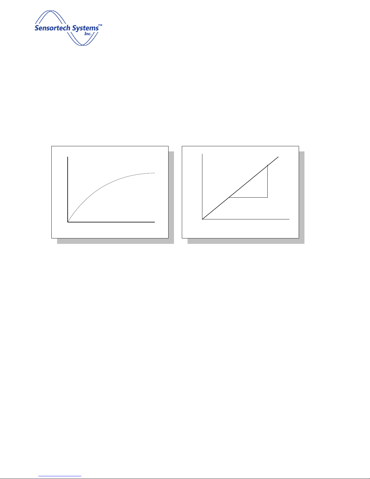
E R U

T S

I O M

5 10 15

INSTRUMENT

Figure 28: Effect of Coefficient B on Slope

E R U

T S

I O M

5 10 15

INSTRUMENT

Figure 29: Effect of Coefficient C on Offset

Offset Mode

The simplest mode of calibration is the ‘Offset’ method. This method assumes that the Sensor has been previously calibrated and the slope (Coefficient B) has already been established. It is primarily intended for online calibration to compensate for process variables such as interface between Sensor and product, density, product height, flow speed, Sensor installation misalignments, etc.

In most cases, the Sensor has been statically calibrated in our factory for your application. Once the Sensor has been installed on-line, a single sample comparison with the measurement value will determine if an offset is necessary.

Screen 37 of 60

ST-3300 Smart RF Sensor Technical Manual

Offset Calibration Procedure

1. Select Calibration Method – Offset Method

2. While material is over the Sensor, press the ‘Start’ button and wait until the measured value is

displayed.

3. Press the ‘Stop’ button and immediately collect a sample from the line at the Sensor and place it in an

airtight container or plastic bag. Completely fill the container and remove any excess air.

4. Press ‘Store Sample’ to record the reading in the Calibration screen data table.

5. Perform a lab analysis on your sample (for moisture this is typically a weight loss oven test), then enter

the lab analysis value into the data table under the ‘Lab’ column.

6. Press ‘Recalculate Coefficients’ and note that the ‘C’ coefficient value has been corrected.

7. Press ‘Send Coefficients’ to conclude the calibration procedure

Linear Mode

Linear regression establishes the direct correlation between two data series. A correlation coefficient indicates the quality of correlation. This value is between 0 and 1, with 1 being perfect.

In addition to determining the quality of fit, the regression function calculates the slope and intercept of the calibration line. These two values are the ‘B’ and ‘C’ coefficients, respectively.

Linear mode should only be used with an adequate range and moisture levels

The following steps will provide an example of how to perform a Product Calibration:

1. Select the Calibration screen tab.

2. Select the constituent to calibrate using the ‘Constituent Select’ drop-down menu.

3. Select the calibration mode using the ‘Calibration Mode’ drop-down menu.

4. Place the sample material to be calibrated under the Sensor Light Tube / Viewing Window.

5. Press the ‘Start’ button. The ‘Sample’ and ‘Average fields will change color to green and the current

measured value is displayed. The ‘Start’ button changes to ‘Stop’ during the measurement.

6. Press the ‘Stop’ button. The ‘Sample’ and ‘Average’ displays will change color to red and the average of

all the readings, obtained during the sample period, is displayed in the ‘Average’ field. The ‘Sample’ field will be cleared. Press ‘Store Sample’ button. The sample measurement is stored to the table.

7. Repeat this procedure to get at least 3 sample measurement readings. A minimum of six sample

measurements is recommended for good calibration data sample set. Samples should be reasonably distributed through the calibration range.

8. The stored samples will be displayed with time and date information in the table fields as shown in

Figure 30.

9. Initially, the ‘Gauge’ value is entered into the ‘Lab’ field also. The actual ‘Lab’ value is manually entered

following the laboratory analysis. Position cursor over desired ‘Lab’ value in table and click field. A data entry window will open to allow entry of the actual ‘Lab’ value.

10. Press the ‘Recalculate Coefficients’ button. The ‘Gauge’ values and the ‘Lab’ values will be used to

recalculate the coefficient values to find the best fit. The new ‘Gauge’ coefficient values appear in the ‘Recalculated’ fields.

Screen 38 of 60

ST-3300 Smart RF Sensor Technical Manual

11. To complete the Product Calibration, click on the ‘Send Coefficients’ button. The new coefficient values

will be sent to the Sensor and overwrite the previous coefficient values stored in the Sensor.

Figure 30: Example of the Calibration Screen after Product Calibration has been performed

The graphical representation is useful in selecting bad data points. If a data point appears to be an outlier it may be temporarily disabled by clicking on the appropriate checkbox in the table. Press ‘Recalculate Coefficients’ button to check if correlation value is significantly improved. If not, uncheck the disable checkbox. If disabling a data point significantly improves correlation, that data point may be permanently removed by highlighting the row in the table and pressing the ‘Delete Sample’ button.

Screen 39 of 60

ST-3300 Smart RF Sensor Technical Manual

Suggestions for taking product samples

a) Take the sample as close to the Sensor as possible. b) Process as large a sample as possible. c) If using damping, take a series of samples over the range of the sampling period. Example: 30 secs damping -

take a sample every 5 secs for 30 seconds.

d) Use a homogenous sample representative of the whole. In the above example, thoroughly mix 30 sec

sample.

e) If using small samples, test samples two or three times (to show repeatability) and average results if

necessary.

f) Use the most accurate testing method available. An oven dry test with a 100g sample is generally more

accurate than a lamp dry test with a 10g sample.

Note: The calibration can only be as accurate as the sampling method.

Screen 40 of 60

Maintenance Screen

ST-3300 Smart RF Sensor Technical Manual

Figure 31: Maintenance Screen for Pre-Zero and Standardize Calibrations

The Maintenance Screen is provided for the user to perform Pre-Zero and Standardize Calibrations of the Sensor during periodic routine maintenance. The user will press the “Pre-ZERO” or “STANDARDIZE” button on the left side of the screen to initiate the Sensor calibration algorithms.

The screen descriptions are as follows (from upper left of Screen):

1. Pre-Zero Button: when pressed performs the Pre-Zero Calibration.

2. Standardize Button: when pressed performs the Standardize Calibration.

3. Current Value: current moisture measurement with B coefficient = 1 and C coefficient = 0.

4. Dz: stored Pre-Zero dielectric value from last Pre-Zero Calibration.

5. Standardization Target 0-100: stored dielectric reference value.

6. Standardization Factor: stored Standardization Factor value from last Standardize Calibration.

Screen 41 of 60

ST-3300 Smart RF Sensor Technical Manual

Pre-Zero Calibration

CAUTION! This is a critical calibration parameter and will affect all calibrations.

The purpose of the Pre-Zero Calibration is to remove the influence of the surrounding environment upon the Sensor e.g. a metal beam located three inches from the face of the Sensor, or a plastic window between Sensor and sample. If this residual dielectric were not negated, it would cause problems when calibrating for product moisture.

The Pre-Zero Calibration allows the user to “Zero” or “Tare” the Sensor after system installation and during routine maintenance. With no product or debris on the Sensor Antenna, the Pre-Zero value is a single dielectric measurement which is stored in memory, this Pre-Zero value is subsequently subtracted from all subsequent measurements.

The value for displayed Moisture is calculated from the equation:

Moisture = STD x B coefficient x (D

Where: B coefficient = slope

calibration coefficient for Product selected (SPAN)

– Pre-Zero) + C coefficient

C coefficient = offset calibration coefficient for Product selected (ZERO) STD = Standardization Factor (calculated) DR = raw dielectric value

Pre-Zero = calculated raw dielectric value with empty Sensor – air only from Pre-Zero Calibration

There are two methods of performing a Pre-Zero Calibration:

1. Using the Configuration Program the user would connect a host PC / laptop to the RS-485 interface and

run the Configuration Program to select the Maintenance Screen to control the Sensor. The user will press the Pre-ZERO button on the Maintenance Screen with nothing over the Sensor to complete the Pre-Zero calibration.

2. The I/O Unit also provides local push button controls for performing the Zero and Standardize

calibrations of the Sensor. The user opens the lid of the enclosure and presses the ZERO button with nothing over the Sensor and the Status LED next to the button lights up to indicate a Pre-Zero calibration has been performed. The Status LED next to the ZERO button lights up to indicate a Standardize calibration has been performed.

Screen 42 of 60

ST-3300 Smart RF Sensor Technical Manual

Standardize Calibration

CAUTION! This is a critical calibration parameter and will affect all calibrations.

DO NOT STANDARDIZE UNIT WITHOUT A STANDARDIZATION PLATE, TUBE, ETC. AS the SENSOR WILL CAUSE ERRONEOUS READINGS. PLEASE CONTACT SENSORTECH SHOULD YOU HAVE ANY QUESTIONS.

The purpose of the Standardize calibration is to provide uniformity of calibration between Sensors, and to provide a repeatable reference for all Sensors at the same location. The Standardization factor, STD is used as a secondary span coefficient, and may be considered as a scaling factor. See following equation:

Moisture = STD * B coefficient * (DR – Pre-Zero) + C coefficient

Where: B coefficient = slope

calibration coefficient for Product selected (SPAN)

C coefficient = offset calibration coefficient for Product selected (ZERO)

STD = Standardization Factor (calculated)

= raw dielectric value

Pre-Zero = calculated raw dielectric value with empty Sensor – air only from Pre-Zero Calibration Due to manufacturing and component tolerances, no two Sensors will be identical. The scaling or Standardization factor will compensate for these differences. During the Standardize calibration, dielectric span is forced to one (1), and dielectric zero forced to zero (0). The equation becomes:

Moisture = STD * (D

– Pre-Zero)

Transposing equation gives:

STD = Moisture / (D

– Pre-Zero)

Using a known dielectric reference, the Standardize calibration allows the user to enter that moisture value and the Sensor will calculate STD value from the above equation. A Standardization Plate or other reference materials are available with very stable dielectrics, which can also be used as dielectric standards

The Standardize Calibration is performed by the user to produce a moisture display value of 25 when a Standardization Plate (dielectric reference) is placed on the Sensor Antenna.

There are two methods of performing a Standardize Calibration:

1. Using the Configuration Program the user would connect a host PC / laptop to the RS-485 interface and

run the Configuration Program to select the Maintenance Screen to control the Sensor. The user places a Standardization Plate over the Sensor and the user will press the STANDARDIZE button on the Maintenance Screen to complete the Standardize calibration.

2. The I/O Unit also provides local push button controls for performing the Zero and Standardize

calibrations of the Sensor. The user would perform the Pre-Zero Calibration followed by the Standardize calibration. The user places a Standardization Plate over the Sensor and the user opens the lid of the enclosure and presses the Standardize button. The Status LED next to the button lights up to indicate a Standardize calibration has been performed.

Screen 43 of 60

ST-3300 Smart RF Sensor Technical Manual

Pre-Zero Calibration Procedure - using the Configuration Program

1. Log in to the Configuration Program using the engineering password. Select the Maintenance Screen.

2. Ensure that the Sensor Antenna is clean, dry and free of debris. No Product or Standardization Plate

should be present on the Sensor Antenna.

3. The ‘Pre-ZERO’ button is pressed on the Maintenance Screen using the Configuration Program. The Pre-

ZERO button will change color to red for several seconds. If there is an error the Current Value field will turn red to indicate a problem occurred.

4. Verify the Current Value displayed equals 0.

If the Current Value displayed is not 0 after the Pre-Zero Calibration do each of the following steps and repeat the Pre-Zero Calibration procedure.

1. Remove all product, debris, Standardization Plate, etc. on the Sensor Antenna. Check the Sensor is

clean and dry.

2. Check the coaxial cables are undamaged, connected and securely tightened on the Sensor

Electronics Unit.

3. Check the M12 cables are undamaged, connected and securely tightened on the Sensor Electronics

Unit and the I/O Unit. Where possible open the enclosures to check for debris or moisture.

Standardize Calibration Procedure - using the Configuration Program

1. Log in to the Configuration Program using the engineering password. Select the Maintenance Screen.

2. Ensure that the Sensor Antenna is clean, dry and free of debris. No Product or Standardization Plate

should be present on the Sensor Antenna.

3. Place the Standardization Plate on conveyor/rollers/belts positioned in the center of Sensor Antenna.

4. The ‘Standardize’ button is pressed on the Maintenance Screen using the Configuration Program. The

Standardize button will change color to red for several seconds. If there is an error the Standardization Factor field will turn red to indicate a problem occurred.

5. Verify the Current Value displayed equals 25. This is the dielectric reference value of the Standardization

Plate.

6. Verify the Standardization Factor value displayed is between 0 – 100.

If the Current Value displayed is not 25 after the Standardize Calibration do each of the following and repeat the Standardize Calibration procedure.

1. Remove all product, debris, Standardization Plate, etc. on the Sensor Antenna. Check the Sensor and

plate are clean and dry. Place the Standardization Plate back over the center of the Sensor Antenna.

2. Check the coaxial cables are undamaged, connected and securely tightened on the Sensor

Electronics Unit.

3. Check the M12 cables are undamaged, connected and securely tightened on the Sensor Electronics

Unit and the I/O Unit. Where possible open the enclosures to check for debris or moisture.

Screen 44 of 60

ST-3300 Smart RF Sensor Technical Manual

Pre-Zero Calibration Procedure - using the I/O Unit Push-buttons

1. Ensure that the Sensor Antenna is clean, dry and free of debris. No Product or Standardization Plate

should be present on the Sensor Antenna.

2. The user opens the lid on the I/O Unit and the ‘ZERO’ pushbutton is pressed and held for 1 second. a. Good Calibration: The STATUS LED will turn green and remain on for several seconds. b. Poor Calibration: the STATUS LED will blink on/off 10 times to indicate a problem occurred.

3. Verify the Current Value displayed equals 0.

If the Current Value displayed is not 0 after the Pre-Zero Calibration, do each of the following steps and repeat the Pre-Zero Calibration procedure.

1. Remove all product, debris, Standardization Plate, etc. on the Sensor Antenna. Check the Sensor is clean

and dry.

2. Check the coaxial cables are undamaged, connected and securely tightened on the Sensor Electronics

Unit.

3. Check the M12 cables are undamaged, connected and securely tightened on the Sensor Electronics Unit

and the I/O Unit. Where possible open the enclosures to check for debris or moisture.

Standardize Calibration Procedure - using the I/O Unit Push-buttons

1. Ensure that the Sensor Antenna is clean, dry and free of debris.

2. Place the Standardization Plate on conveyor/rollers/belts positioned in the center of Sensor Antenna.

3. The user opens the lid on the I/O Unit and the ‘ZERO’ pushbutton is pressed and held for 1 second. a. Good Calibration: The STATUS LED will turn green and remain on for several seconds. b. Poor Calibration: the STATUS LED will blink on/off 10 times to indicate a problem occurred

4. Verify the Current Value displayed equals 25. This is the dielectric reference value of the Standardization

Plate.

5. Verify the Standardization Factor value displayed is between 0 – 100.

If the Current Value displayed is not 25 or the Standardization Factor less than 0 or greater than 100 after the Standardize Calibration do each of the following and repeat the Standardize Calibration procedure.

1. Remove all product, debris, Standardization Plate, etc. on the Sensor Antenna. Check the Sensor and

plate are clean and dry. Place the Standardization Plate back over the center of the Sensor Antenna.

2. Check the coaxial cables are undamaged, connected and securely tightened on the Sensor Electronics

Unit.

3. Check the M12 cables are undamaged, connected and securely tightened on the Sensor Electronics Unit

and the I/O Unit. Where possible open the enclosures to check for debris or moisture.

Screen 45 of 60

ST-3300 Smart RF Sensor Technical Manual

Appendix

Sensor Electronics Unit External Connectors

The Sensor Electronics Unit external connectors are industry standard M12 type cables for water and dust protection.

M12 x 12 Pin Connector

Pin Signal Name Signal Description

1 4-20mA Out - Moisture or Product Temperature measurement negative output

2 -15VDC -15VDC power input @ 1A

3 Ground +/-15V Ground

4 Ground +/-15V Ground

5 +15VDC +15VDC power input @ 1A

6 OP+ RS-485 Positive Output

7 OP- RS-485 Negative Output 8 IP- RS-485 Negative Input

9 G RS-485 Ground

10 4-20mA Out + Moisture or Product Temperature measurement positive output

11 +15VDC +15VDC power input @ 1A 12 IP+ RS-485 Positive Input

M12 x 8 Pin Connector

Pin Signal Name Signal Description

1 DIG_IN+ External Gate Control Positive Digital Input ( 0-24V @ 0.05A)

2 STANDARDIZE External Open Collector Input for Standardize Calibration (0V input = perform Standardize Calibration)

3 STATUS LED External LED Status Indicator Output (0-3.3V output @ 0.02A)

4 ZERO External Open Collector Input for Pre-Zero Calibration (0V input = perform Pre-Zero Calibration)

5 DIG_IN- External Gate Control Negative Digital Input ( 0-24V @ 0.05A)

6 Ground System Ground

7 +15VDC +15VDC power output @ 0.1A 8 N/C No connect

M12 x 4 Pin Connector

Pin Signal Name Signal Description

1 PROD_TEMP_IN Product Temperature measurement positive input (configurable for 4-20mA or 0-1VDC input)

2 Ground +15V Ground

3 +15VDC +15VDC power output @ 0.1A

4 N/C No connect

Screen 46 of 60

ST-3300 Smart RF Sensor Technical Manual

I/O Unit External Connectors

The I/O Unit external connectors are industry standard M12 type cables for water and dust protection.

M12 x 12 Pin Connector

Pin Signal Name Signal Description

1 4-20mA Out - Moisture or Product Temperature Measurement 4-20mA Negative Output Feedthru

2 -15VDC -15VDC Power Supply Output @ 1A

3 Ground +/-15V Ground

4 Ground +/-15V Ground

5 +15VDC +15VDC Power Supply Output @ 1A

6 OP+ RS-485 Positive Output Feedthru

7 OP- RS-485 Negative Output Feedthru 8 IP- RS-485 Negative Input Feedthru

9 G RS-485 Ground

10 4-20mA Out + Moisture or Product Temperature Measurement 4-20mA Positive Output Feedthru

11 +15VDC +15VDC Power Supply Output @ 1A 12 IP+ RS-485 Positive Input Feedthru

M12 x 8 Pin Connector

Pin Signal Name Signal Description

1 DIG_IN+ External Gate Control Positive Digital Feedthru

2 STANDARDIZE Open Collector Output for Standardize Calibration (0V output = perform Standardize Calibration)

3 STATUS LED External LED Status Indicator Input (0-3.3V output @ 0.02A)

4 ZERO Open Collector Output for Pre-Zero Calibration (0V output = perform Pre-Zero Calibration)

5 DIG_IN- External Gate Control Negative Digital Feedthru

6 Ground System Ground

7 +15VDC +15VDC Power Input 8 N/C No connect

Screen 47 of 60

I/O Unit Terminal Board Layout

ST-3300 Smart RF Sensor Technical Manual

Figure 32: I/O Unit Terminal Board Layout

Figure 33:.

Screen 48 of 60

I/O Unit Terminal Board Signals

I/O Unit Connector/Terminal Block Signals

Internal Signal

Connector

Pin External Signal

External Signal Description

OP- J3 2 Users RS

485 RxD

- To

Users

Host PC or Connector J4

OP+

J3 Users RS

485 RxD+

Users

Host PC or Connector J4

IP+ J3

Users RS

485 TxD+

Users

Host PC or Connector J4

IP- J3 Users RS

485 TxD

- To

Users

Host PC or Connector J4

G J3 Users RS

485 Ground

Users

Host PC or Connector J4

I/O Unit Internal +15VDC (< 100mA) to power

I/O

Unit Internal Ground to power Proximity

Proximity Detector or Micro

Switch Output for

Proximity Detector or Micro

Switch Output for

User PLC/Controller

Moisture or Product Temperature measurement

User PLC/Controller

Moisture or Product Temperature measurement

Users RS

485 Bus B

OP- J7 2 Users RS

485 Bus B RxD

- Users PLC/Controller RS

485 RxD

- OP+

J7 3

Users RS

485 Bus B RxD+

Users PLC/Controller RS

485 RxD+

IP+ J7 4 Users RS

485 Bus B TxD+

Users PLC/Controller RS

485 TxD+

IP- J7 5

Users RS

485 Bus B TxD

- Users PLC/Controller RS

485 TxD

Users RS

485 Bus A

OP- J8 2 Users RS

485 Bus A RxD

- Users PLC/Controller RS

485 RxD

- OP+

J8 3

Users RS

485 Bus A RxD+

Users PLC/Controller RS

485 RxD

IP+ J8 4 Users RS

485 Bus A TxD+

Users PLC/Controller RS

485 TxD+

IP- J8 5

Users RS

485 Bus A TxD

- Users PLC/Controller RS

485 TxD

Safety Ground

J9 1

Safety Ground

(90-250VAC 50

60Hz)

Line / Hot

J9 2

Line / Hot

Line / Hot (90

250VAC 50

60Hz)

Neutral

J9 3

Neutral

Neutral (90

250VAC 50

60Hz)

ST-3300 Smart RF Sensor Technical Manual

+15VDC J5 1 Digital Input +15VDC

Ground J5 2 Digital Input Ground

Dig In + J5 3 Digital Output+

Dig In - J5 4 Digital Output-

4-20mA Out + J6 1

4-20mA Out - J6 2

G J7 1

Positive 4-20mA Input

Negative 4-20mA Input

Ground User PLC/Controller RS-485 Ground

Proximity Detector or Micro-Switch

Detector or Micro-Switch

gated measurement control

output value

G J8 1

Ground Users PLC/Controller RS-485 Ground

Screen 49 of 60

ST-3300 Smart RF Sensor Technical Manual

Sensor Status and Error Messages

The Configuration Program displays Sensor status and messages on the lower bar of the display screens.

Configuration Program Message

Displayed

Connected – Measure Sensor operating normally. Sample measurement in range.

Sampling Stopped

Not Connected Configuration program not connected to the Sensor.

Measure Data Received

Measure Data Sent

Measure Data Error

TIMED_MODE_FILL

TIMED_MODE_PURGE In Timed Sample mode. Purging last sample from sample cup.

Connected – NO_GATE

Sensor operating normally. Hold last sample measurement or measurement not Started on Main Screen.

Screen update data received by Sensor from the Host PC/Controller. The Sensor is operating normally.

Screen update data sent to Host PC/Controller from the Sensor. The Sensor is operating normally.

Screen update data not sent or received from Sensor. The Sensor is operating normally but data may need to be re-sent or re-read.

In Timed Sample Mode. Holding last sample measurement while sample cup is being filled.

In Signal Gated sample mode. Holding last sample measurement until signal gate level goes high or measurement threshold is exceeded.

Message Description

Screen 50 of 60

ST-3300 Smart RF Sensor Technical Manual

ST-3300 Sensor RS-485 Communications Interface Specification

Sensortech Systems, Inc. is disclosing this manual to you solely for use to operate with Sensortech hardware devices. You may not reproduce, distribute, republish, download, display, post, or transmit the documentation in any form or by any means including, but not limited to, electronic, mechanical, photocopying, recording, or otherwise, without the prior written consent of Sensortech Systems. Sensortech Systems expressly disclaims any liability arising out of your use of the documentation. Sensortech Systems reserves the right, at its sole discretion, to change the documentation without notice at any time. Sensortech Systems assumes no obligation to correct any errors contained in the documentation, or to advise you of any corrections or updates. Sensortech Systems expressly disclaims any liability in connection with technical support or assistance that may be provided to you in connection with the information.

THE DOCUMENTATION IS DISCLOSED TO YOU “AS-IS” WITH NO WARRANTY OF ANY KIND. SENSORTECH SYSTEMS MAKES NO OTHER WARRANTIES, WHETHER EXPRESS, IMPLIED, OR STATUTORY, REGARDING THE DOCUMENTATION, INCLUDING ANY WARRANTIES OF MERCHANTABILITY, FITNESS FOR A PARTICULAR PURPOSE, OR NONINFRINGEMENT OF THNIRD PARTY RIGHTS. IN NO OCCURRENCE WILL SENSORTECH SYSTEMS BE LIABLE FOR ANY CONSEQUENTIAL, INDNIRECT, EXEMPLARY, SPECIAL, OR INCIDENTAL DAMAGES, INCLUDING ANY LOSS OF DATA OR LOST PROFITS, ARISING FROM YOUR USE OF THE DOCUMENTATION.

Sensortech, the Sensortech logo, and other designated brands included herein are trademarks of Sensortech Systems, Inc. All other trademarks are the property of their respective owners.

ST-3300 MODBUS-RTU Serial Communications Interface

External devices can communicate with the ST-3300 via Serial RS485 using a simple Modbus RTU protocol

The ST-3300 Modbus RTU protocol is very simple. It is further simplified by the fact that we support only two Modbus function codes - 03 (Multiple Register Read) and 16 (Multiple Register Write).

For function code 03, the host computer sends out: Slave Address (8 bits) – the gauge address set in the serial configuration screen Function Code (8 bits. Value = 03) Start Address (High byte) Start Address (Low Byte) normally set to 0 Number of registers (High byte)

Screen 51 of 60

ST-3300 Smart RF Sensor Technical Manual

Number of registers (Low byte) normally set to 16 CRC (16 bits) The gauge responds with: Slave Address (8 bits) Function Code (8 bits. Value = 03) Byte Count (8 bits) (2* number of registers) normally 32 Data High Data Low ... Data High Data Low CRC (16 bits) For function code 16, the host computer sends out: Slave Address (8 bits) – the gauge address set in the serial configuration screen Function Code (8 bits. Value = 16) Start Address (High byte) Start Address (Low Byte) normally 0 Number of registers (High byte) Number of registers (Low byte) normally 4 Byte Count (8 bits) (2* number of registers) normally 8 Data High Data Low ... Data High Data Low CRC (16 bits) The gauge responds with: Slave Address (8 bits) Function Code (8 bits. Value = 03) Start Address (High byte) Start Address (Low Byte) Number of registers (High byte) Number of registers (Low byte) CRC (16 bits)

CRC Generation, Code Examples

CRC Calculation Basics

The CRC calculation is started by first preloading a 16-bit register to all 1's. Then a process begins of applying successive eight-bit bytes of the message to the current contents of the register. During generation of the CRC, each eight-bit character is XOR’d with the current register contents. The result is shifted in the direction of the least significant bit (LSB), with a zero filled into the most significant bit (MSB) position. The LSB is extracted and examined. If the LSB is a 1, the register is XOR’d with a preset, fixed value. If the LSB was a 0, no XOR takes place. This process is repeated until eight shifts have been

Screen 52 of 60

ST-3300 Smart RF Sensor Technical Manual

performed. After the last (eighth) shift, the above process repeats for the next byte in the message. The final contents of the register, after all bytes of the message have been applied, is the CRC value.

Step by Step:

1. Load a 16-bit register with 0xFFFF (all 1's). Call this the CRC register

2. XOR the first eight-bit byte of the message with the low order byte of the 16-bit CRC register, putting the result in the CRC register

3. Shift the CRC register one bit to the right (toward the LSB), zerofilling the MSB. Extract and examine the LSB

4. If the LSB is 0, repeat Step 3 (another shift). If the LSB is 1, Exclusive OR the CRC register with the polynomial value 0xA001 (1010 0000 0000 0001)

5. Repeat Steps 3 and 4 until eight shifts have been performed. When this is done, a complete eight bit byte will have been processed

6. Repeat Steps 2 … 5 for the next eight-bit byte of the message. Continue doing this until all Bytes have been processed.

• Result The final contents of the CRC register is the CRC value. When the CRC is placed into the message, its upper and lower bytes must be swapped as described in chapter 9-1 “Modbus Protocol” (CRC).

Screen 53 of 60

ST-3300 Smart RF Sensor Technical Manual

Example 1

The following example calculates the CRC using the method described earlier. Note: This function performs the swapping of the high/low CRC bytes internally. Therefore the CRC value returned from the function can be directly placed into the message for transmission. The function returns the CRC as a type UINT16, and takes two arguments:

• UINT8 *pabMessage;

A pointer to the message buffer containing binary data to be used for generating the CRC.

• UINT16 iLength;

The quantity of bytes in the message buffer.

Typedefs

UINT8 = Unsigned 8 bit ( e.g. unsigned char ) UINT16 = Unsigned 16 bit ( e.g. unsigned short )

Source Code

UINT16 GenerateCrc( UINT8* pabMessage, UINT16 iLength ) { UINT16 iCRCReg = 0xFFFF; UINT8 bByteCount; UINT8 bBitCount, bCarryFlag; for( bByteCount = 0 ; bByteCount < iLength ; bByteCount++ ) { *((UINT8*)&iCRCReg + 1) = pabMessage[ bByteCount ] ^ ( iCRCReg & 0x00FF ); for( bBitCount = 0; bBitCount < 8 ; bBitCount++ ) { bCarryFlag = iCRCReg & 0x0001; iCRCReg = iCRCReg >> 1; if( bCarryFlag != 0 ) { iCRCReg ^= 0xA001; } } } return( iCRCReg << 8 | iCRCReg >> 8 ); }/* end GenerateCrc */

Example 2

This example uses another approach to calculate the CRC; All of the possible CRC values are Preloaded into two arrays, which are simply indexed as the function increments through the message buffer. One array contains all of the 256 possible CRC values for the high byte of the 16-bit CRC field, and the other array contains all of the values for the low byte. Indexing the CRC in this way provides faster execution than would be achieved by calculating a new CRC value with each new character from the message buffer. Note: This function performs the swapping of the high/low CRC bytes internally. Therefore the CRC value returned from the function can be directly placed into the message for transmission. The function returns the CRC as a type UINT16, and takes two arguments:

Screen 54 of 60

ST-3300 Smart RF Sensor Technical Manual

• UINT8 *pabMessage; A pointer to the message buffer containing binary data to be used for generating the CRC.

• UINT16 iLength; The quantity of bytes in the message buffer. Typedefs UINT8 = Unsigned 8 bit ( e.g. unsigned char ) UINT16 = Unsigned 16 bit ( e.g. unsigned short ) CRC Generation, Code Examples B-4 Source Code UINT16 GenerateCrc( UINT8* pabMessage, UINT16 iLength ) { static UINT8 abCrcHi[] = { 0x00, 0xC1, 0x81, 0x40, 0x01, 0xC0, 0x80, 0x41, 0x01, 0xC0, 0x80, 0x41, 0x00, 0xC1, 0x81, 0x40, 0x01, 0xC0, 0x80, 0x41, 0x00, 0xC1, 0x81, 0x40, 0x00, 0xC1, 0x81, 0x40, 0x01, 0xC0, 0x80, 0x41, 0x01, 0xC0, 0x80, 0x41, 0x00, 0xC1, 0x81, 0x40, 0x00, 0xC1, 0x81, 0x40, 0x01, 0xC0, 0x80, 0x41, 0x00, 0xC1, 0x81, 0x40, 0x01, 0xC0, 0x80, 0x41, 0x01, 0xC0, 0x80, 0x41, 0x00, 0xC1, 0x81, 0x40, 0x01, 0xC0, 0x80, 0x41, 0x00, 0xC1, 0x81, 0x40, 0x00, 0xC1, 0x81, 0x40, 0x01, 0xC0, 0x80, 0x41, 0x00, 0xC1, 0x81, 0x40, 0x01, 0xC0, 0x80, 0x41, 0x01, 0xC0, 0x80, 0x41, 0x00, 0xC1, 0x81, 0x40, 0x00, 0xC1, 0x81, 0x40, 0x01, 0xC0, 0x80, 0x41, 0x01, 0xC0, 0x80, 0x41, 0x00, 0xC1, 0x81, 0x40, 0x01, 0xC0, 0x80, 0x41, 0x00, 0xC1, 0x81, 0x40, 0x00, 0xC1, 0x81, 0x40, 0x01, 0xC0, 0x80, 0x41, 0x01, 0xC0, 0x80, 0x41, 0x00, 0xC1, 0x81, 0x40, 0x00, 0xC1, 0x81, 0x40, 0x01, 0xC0, 0x80, 0x41, 0x00, 0xC1, 0x81, 0x40, 0x01, 0xC0, 0x80, 0x41, 0x01, 0xC0, 0x80, 0x41, 0x00, 0xC1, 0x81, 0x40, 0x00, 0xC1, 0x81, 0x40, 0x01, 0xC0, 0x80, 0x41, 0x01, 0xC0, 0x80, 0x41, 0x00, 0xC1, 0x81, 0x40, 0x01, 0xC0, 0x80, 0x41, 0x00, 0xC1, 0x81, 0x40, 0x00, 0xC1, 0x81, 0x40, 0x01, 0xC0, 0x80, 0x41, 0x00, 0xC1, 0x81, 0x40, 0x01, 0xC0, 0x80, 0x41, 0x01, 0xC0, 0x80, 0x41, 0x00, 0xC1, 0x81, 0x40, 0x01, 0xC0, 0x80, 0x41, 0x00, 0xC1, 0x81, 0x40, 0x00, 0xC1, 0x81, 0x40, 0x01, 0xC0, 0x80, 0x41, 0x01, 0xC0, 0x80, 0x41, 0x00, 0xC1, 0x81, 0x40, 0x00, 0xC1, 0x81, 0x40, 0x01, 0xC0, 0x80, 0x41, 0x00, 0xC1, 0x81, 0x40, 0x01, 0xC0, 0x80, 0x41, 0x01, 0xC0, 0x80, 0x41, 0x00, 0xC1, 0x81, 0x40 }; static UINT8 abCrcLo[] = { 0x00, 0xC0, 0xC1, 0x01, 0xC3, 0x03, 0x02, 0xC2, 0xC6, 0x06, 0x07, 0xC7, 0x05, 0xC5, 0xC4, 0x04, 0xCC, 0x0C, 0x0D, 0xCD, 0x0F, 0xCF, 0xCE, 0x0E, 0x0A, 0xCA, 0xCB, 0x0B, 0xC9, 0x09, 0x08, 0xC8, 0xD8, 0x18, 0x19, 0xD9, 0x1B, 0xDB, 0xDA, 0x1A, 0x1E, 0xDE, 0xDF, 0x1F, 0xDD, 0x1D, 0x1C, 0xDC, 0x14, 0xD4, 0xD5, 0x15, 0xD7, 0x17, 0x16, 0xD6, 0xD2, 0x12, 0x13, 0xD3, 0x11, 0xD1, 0xD0, 0x10, 0xF0, 0x30, 0x31, 0xF1, 0x33, 0xF3, 0xF2, 0x32, 0x36, 0xF6, 0xF7, 0x37, 0xF5, 0x35, 0x34, 0xF4, 0x3C, 0xFC, 0xFD, 0x3D, 0xFF, 0x3F, 0x3E, 0xFE, 0xFA, 0x3A, 0x3B, 0xFB, 0x39, 0xF9, 0xF8, 0x38, 0x28, 0xE8, 0xE9, 0x29, 0xEB, 0x2B, 0x2A, 0xEA, 0xEE, 0x2E, 0x2F, 0xEF, 0x2D, 0xED, 0xEC, 0x2C, 0xE4, 0x24, 0x25, 0xE5, 0x27, 0xE7, 0xE6, 0x26,

Screen 55 of 60

ST-3300 Smart RF Sensor Technical Manual

0x22, 0xE2, 0xE3, 0x23, 0xE1, 0x21, 0x20, 0xE0, 0xA0, 0x60, 0x61, 0xA1, 0x63, 0xA3, 0xA2, 0x62, 0x66, 0xA6, 0xA7, 0x67, 0xA5, 0x65, 0x64, 0xA4, 0x6C, 0xAC, 0xAD, 0x6D, 0xAF, 0x6F, 0x6E, 0xAE, 0xAA, 0x6A, 0x6B, 0xAB, 0x69, 0xA9, 0xA8, 0x68, 0x78, 0xB8, 0xB9, 0x79, 0xBB, 0x7B, 0x7A, 0xBA, 0xBE, 0x7E, 0x7F, 0xBF, 0x7D, 0xBD, 0xBC, 0x7C, 0xB4, 0x74, 0x75, 0xB5, 0x77, 0xB7, 0xB6, 0x76, 0x72, 0xB2, 0xB3, 0x73, 0xB1, 0x71, 0x70, 0xB0, 0x50, 0x90, 0x91, 0x51, 0x93, 0x53, 0x52, 0x92, 0x96, 0x56, 0x57, 0x97, 0x55, 0x95, 0x94, 0x54, 0x9C, 0x5C, 0x5D, 0x9D, 0x5F, 0x9F, 0x9E, 0x5E, 0x5A, 0x9A, 0x9B, 0x5B, 0x99, 0x59, 0x58, 0x98, 0x88, 0x48, 0x49, 0x89, 0x4B, 0x8B, 0x8A, 0x4A, 0x4E, 0x8E, 0x8F, 0x4F, 0x8D, 0x4D, 0x4C, 0x8C, 0x44, 0x84, 0x85, 0x45, 0x87, 0x47, 0x46, 0x86, 0x82, 0x42, 0x43, 0x83, 0x41, 0x81, 0x80, 0x40 }; UINT8 bCrcHi = 0xFF; UINT8 bCrcLo = 0xFF; UINT16 iIndex; while( iLength-- ) { iIndex = bCrcHi ^ *pabMessage++; bCrcHi = bCrcLo ^ abCrcHi[iIndex]; bCrcLo = abCrcLo[iIndex]; } return( bCrcHi << 8 | bCrcLo ); }/* end GenerateCrc */

Read Only Messages

Data Object: Measurement Data Modbus Address: 0x10 Data Size (Bytes): 12 - Read Only

Data Definition: Moisture Value – IEEE float (4 bytes) Temperature Value – IEEE float (4 bytes) Measurement Status – unsigned 32 bit integer (4 bytes) 0 = No Errors Bit 0-31 definitions: Bit 0 Set = 3.3 Volt Error Bit 1 Set = 5 Volt Error Bit 2 Set = 12 Volt Error Bit 3 Set = -12 Volt Error Bit 4 Set = Board Temperature Alarm Bit 5 Set = Reference Frequency Error Bit 6 Set = Bad Zero Bit 7 Set = Bad Standardization Bits 8-31 reserved for future use

Screen 56 of 60

Data Object: Sensor Information Modbus Address: 0x20 - Read Only Data Size (Bytes): 20

Data Definition: Serial Number – unsigned 32 bit integer (4 bytes) Model – ASCII string (10 bytes) Hardware Major Version – ASCII character (1 byte) Hardware Major Minor – numeric byte value (1 byte) Firmware Version – IEEE float (4 bytes)

Data Object: Diagnostics Data Modbus Address: 0x150 - Read Only Data Size (Bytes): 72

Data Definition: Frequency Fs – unsigned 32 bit integer (4 bytes) Frequency Fl – unsigned 32 bit integer (4 bytes) Frequency Fh – unsigned 32 bit integer (4 bytes) Dr – IEEE float (4 bytes) Dz – IEEE float (4 bytes) Standardization – IEEE float (4 bytes) Board Temperature – IEEE float (4 bytes) Moisture – IEEE float (4 bytes) Uncalibrated Moisture – IEEE float (4 bytes) Voltage 3.3V – IEEE float (4 bytes) Voltage 5V – IEEE float (4 bytes) Voltage 12V – IEEE float (4 bytes) Voltage -12V – IEEE float (4 bytes) Product Temperature – IEEE float (4 bytes) Digital Input 1 - unsigned 16 bit integer (2 bytes) Digital Input 2 - unsigned 16 bit integer (2 bytes) Future Use - unsigned 16 bit integer (2 bytes) Future Use - unsigned 16 bit integer (2 bytes) Error Status - unsigned 32 bit integer (4 bytes) 0 = No Errors

Bit 0-31 definitions: Bit 0 Set = 3.3 Volt Error Bit 1 Set = 5 Volt Error Bit 2 Set = 12 Volt Error Bit 3 Set = -12 Volt Error Bit 4 Set = Board Temperature Alarm Bit 5 Set = Reference Frequency Error Bit 6 Set = Bad Zero Bit 7 Set = Bad Standardization Bits 8-31 reserved for future use

Future Use - unsigned 32 bit integer (4 bytes)

ST-3300 Smart RF Sensor Technical Manual

Screen 57 of 60

ST-3300 Smart RF Sensor Technical Manual

Write Only Messages

Data Object: Pre-Zero Command – Sending this message causes the Sensor to perform a Pre-Zero Modbus Address: 0x60 - Write Only Data Size (Bytes): 2

Data Definition: Dummy Value - unsigned 16 bit integer (2 bytes) Set to 0x5555

Data Object: Standardization Command – Sending this message causes the Sensor to perform a Standardization Modbus Address: 0x65 - Write Only Data Size (Bytes): 2

Data Definition: Dummy Value - unsigned 16 bit integer (2 bytes) Set to 0xAAAA

Read/Write Data Objects

The following read/write data objects are read in a single multiple register read and written in a single multiple register write – no individual registers within a group are readable or writable. All registers in the write object have to contain valid data. The best way to change parameters is to perform a read-modify-write: first read the data object into a buffer, modify the parameters that need to be changed, and then write the entire data object back.

Data Object: Product Code Read/Change Active Product Code

Modbus Address: 0x50 Read/Write Data Size (Bytes): 2

Data Definition: Product Code – 16 bit integer (2 bytes) – the current product code 0-50

Data Object: Measure Configuration Data Modbus Address: 0x300 Read/Write Data Size (Bytes): 30

Data Definition: Measurement Mode – 16 bit integer (2 bytes) 0 – default – Continuous

1- Signal Gated 2- Automatic Product Detect 3- Timed Sample 4- Gated Timed Sample 5- Auto Reference

Sample Period – 16 bit integer (2 bytes) Milliseconds: 5, 10(default), 20, 50, 100 Sensor Measurements– 16 bit integer (2 bytes) Sensor measurements per cycle 1-500, default: 98

Screen 58 of 60

Reference Measurements– 16 bit integer (2 bytes) Default: 1 Reference Moisture – 16 bit integer (2 bytes) 1-100 default: 25 Median Filter Size – 16 bit integer (2 bytes) 1-31 default: 5 Mean Filter Size – 16 bit integer (2 bytes) 1-100 default: 1 Damping Size – 16 bit integer (2 bytes) 1-500 default: 1 Damping Bypass – 16 bit integer (2 bytes) 1-100 default:100 Batch Mode – 16 bit integer (2 bytes) 1 = Batch Mode Fill Time – 16 bit integer (2 bytes) Used in timed sample modes Seconds - default: 10 Measure Time – 16 bit integer (2 bytes) Used in timed sample modes Seconds - default: 2 Purge Time – 16 bit integer (2 bytes) Used in timed sample modes Seconds - default: 2 Product Loss Threshold – IEEE float (4 bytes) Used in Auto Detect Mode

Data Object: Serial and 4-20mA Configuration Modbus Address: 0x550 Read/Write Data Size (Bytes): 72

Data Definition: Baud Rate 16 bit integer (2 bytes) Note: Baud Rate currently fixed at 115200 Modbus Address - 16 bit integer (2 bytes) Data I/O bit 1 mode - 16 bit integer (2 bytes) TBD Data I/O bit 2 mode - 16 bit integer (2 bytes) TBD Port1 4-20mA Select - 16 bit integer (2 bytes) 0 = Moisture 1 = Product Temperature Port2 4-20mA Select - 16 bit integer (2 bytes) 0 = Moisture 1 = Product Temperature Port1 4mA Level – IEEE float (4 bytes) 0-100 Port1 20mA Level – IEEE float (4 bytes) 0-100

ST-3300 Smart RF Sensor Technical Manual

Screen 59 of 60

Port2 4mA Level – IEEE float (4 bytes) 0-100 Port2 20mA Level – IEEE float (4 bytes) 0-100

Data Object: Product Code Calibration Configuration Modbus Address: 0x600 Read/Write Data Size (Bytes): 72

Data Definition: Product Code (0-49)– 16 bit integer (2 bytes) Coefficient B (span) - IEEE float (4 bytes) Coefficient C– (zero) - IEEE float (4 bytes) Alarm Limit 1 - IEEE float (4 bytes) Alarm Limit 2– IEEE float (4 bytes) Product Code Description – character string (100bytes)

ST-3300 Smart RF Sensor Technical Manual

Screen 60 of 60

Sensortech Systems ST-3300 Series Technical Manual

Specifications and Main Features

Frequently Asked Questions

User Manual